Foundations of Agnostic Statistics (Cambridge University Press, 2019) is a textbook on what can be learned from data without assuming that a parametric model is true. It treats regression and maximum likelihood as plug-in estimators of best approximations, and it separates identification from estimation. 126 entries are classified as errors (8 Moderate, 118 Minor, none Major or Critical), and 24 are clarity notes. The most consequential is P001-C07-E011: the book says that the bootstrap standard errors are likely to be adequate for nearest-neighbor matching, but the bootstrap variance of a matching estimator can be inconsistent even when the estimator has no bias.
What was and was not checked
I examined the whole book: the front matter, the seven chapters, the two glossaries, the references and the index. The list below states what I examined and what held up. It is not a finding that the rest of the book is correct.
Statements and proofs. I followed the proofs of the following results step by step. They hold as printed, apart from misprints reported as separate findings: the basic properties of probability and the addition rule (Theorems 1.1.4 and 1.1.7); the Law of Iterated Expectations, the Law of Total Variance and the properties of deviations from the CEF (Theorems 2.2.17 to 2.2.19); the unbiasedness, sampling variance and Chebyshev bound for the sample mean, and the Weak Law of Large Numbers (Theorems 3.2.3 to 3.2.5 and 3.2.8); the OLS solution and the properties of its residuals (Theorems 4.1.4 and 4.1.5); polynomial approximation of the CEF (Theorem 4.3.3); sharp bounds, identification under MCAR and MAR, the propensity score and double robustness for missing data (Theorems 6.1.3, 6.1.6, 6.1.9, 6.1.10, 6.1.12 and 6.2.9); and the corresponding causal results (Theorems 7.1.7, 7.1.13, 7.1.14, 7.1.16, 7.2.5 and 7.2.8).
Worked examples. I recomputed the following numerical examples exactly; their results hold apart from corrections reported separately: the example of the coin flip and die roll in Chapter 1 (P(B)=5/24 and P(A∣B)=3/5), Example 2.2.23 (β=10 and α=−5/3), the regression fitted to the 15 rows of Table 4.1.1 (3.52 and 1.04), and the imputation and matching examples of Chapters 6 and 7 (Examples 6.2.3, 6.2.5 and 7.2.4).
Simulation tables. I independently reproduced all 18 cells of Table 3.4.1 by simulation with 106 replications for each n, with agreement within rounding and Monte Carlo error. I compared all 18 cells of Table 3.4.2 with an exact binomial computation; they agree within rounding and the Monte Carlo error of the published 106 replications.
Empirical tables. Tables 4.4.5, 6.3.1 and 7.5.1 are internally consistent, and the numbers quoted from them in the text match the tables, apart from findings reported separately.
Front and back matter. The entries of the Contents and the 36 entries of the list of tables and figures agree with the body in wording and page number. The 18 entries of the Glossary of Common Abbreviations expand correctly and point to the stated items. Every identifiable in-text citation has an entry in the References; the citation on p. 177 lacks its author and cannot be matched to a work (P001-C04-N016). Every entry is cited at least once.
I did not complete the following checks.
I did not have replication code for the book, the Quality of Government data used in Chapters 4 and 6, or the naturalization data of Hainmueller and Hangartner used in Chapter 7. No estimate, standard error or figure drawn from data in Sections 4.4, 6.3 or 7.5 was reproduced.
I did not have the code that produced the simulated figures. I compared figures with the stated formulas where that was possible.
I read only a few of the works cited by the book to settle specific points. I did not systematically check bibliographic details against the publications themselves; the individual entries document the specific checks I made.
I did not check the historical and biographical statements in the front matter against outside sources, except for one spelling in the acknowledgments.
Six possible errors could not be settled with the sources available. Two concern citations (a year, and several chapter and page references). Two concern whether figures were drawn from the designs stated in the text (Figures 4.3.4, 4.3.5 and 7.3.2). One concerns the definition of the water-access variable in Section 4.4, and one concerns the first year of the sample in Section 7.5.
Headline claims and related corrections
The Glossary of Mathematical Notation defines, with worked examples, the common notation that the main text uses without defining it.
Glossary of Mathematical Notation, table on pp. 282-285 (PDF pp. 300-303); opening sentence on p. 282; Introduction p. xviii
The Glossary of Common Abbreviations gives the unabbreviated form of the abbreviations used in the book and points to where each is defined; abbreviated terms are defined at first use in the text.
Glossary of Common Abbreviations, table on pp. 286-287 (PDF pp. 304-305); sentence above the table on p. 286; Introduction p. xviii (“gives the meanings of all common abbreviations used in this book, along with references to where they are defined in the text”)
Random generative processes are formalized as probability spaces, and the Kolmogorov axioms imply monotonicity, the subtraction rule, P(∅)=0, the bounds 0≤P(A)≤1, the complement rule and the addition rule.
Definitions 1.1.1-1.1.2; Theorems 1.1.4 and 1.1.7; Examples 1.1.3 and 1.1.6
Conditional probability satisfies the Multiplicative Law, Bayes' Rule and the Law of Total Probability. Events A and B are independent when P(A∩B)=P(A)P(B), equivalently P(A∣B)=P(A) when P(B)>0. In the coin-and-die example, P(B)=5/24 and P(A∣B)=3/5, and heads is independent of neither a roll of 3 nor a roll of 6.
Random variables, functions of them and operators on them are mathematical objects; two random variables are equal when they agree at every outcome, and g(X)=h(X) if and only if g and h agree on the range X(Ω).
Definitions 1.2.1-1.2.3 and 1.3.1; Theorem 1.3.2; footnote 28
The PMF characterizes a discrete distribution and the CDF a general distribution. For a continuous variable, the book states that the PDF is unique and equals dF/dx at every x, its integral gives interval probabilities, and Pr[X=x]=0. The support is defined as the set where the PMF or PDF is positive.
Joint PMFs, PDFs and CDFs describe bivariate distributions and yield marginal and conditional distributions and event probabilities. The book characterizes independence of X and Y by factorization of the joint PMF or PDF into the marginals, by the corresponding conditional distributions, by independence of all events {X∈D} and {Y∈E}, and by independence of g(X) and h(Y) for all functions g and h.
Expected values, moments, variances and standard deviations summarize a distribution without a parametric model. Expectations are linear: E[c]=c, E[aX]=aE[X] and E[aX+bY+c]=aE[X]+bE[Y]+c. Expectations of functions can be computed from the PMF or PDF. The variance and standard-deviation rules include V[X]=E[X2]−E[X]2, V[X+c]=V[X], V[aX]=a2V[X] and σ[aX]=∣a∣σ[X]. Chebyshev's inequality bounds the probability of a deviation of at least ϵ standard deviations by 1/ϵ2; a normal distribution is determined by its mean and standard deviation and is closed under affine maps and independent sums.
Definitions 2.1.1, 2.1.10-2.1.12, 2.1.15, 2.1.19; Theorems 2.1.5, 2.1.6, 2.1.8, 2.1.9, 2.1.13-2.1.18, 2.1.20, 2.1.21; Examples 2.1.2-2.1.4, 2.1.17 (printed pp. 44-56, PDF pp. 62-74)
The mean squared error of X about c is V[X]+(E[X]−c)2, so the expected value is the constant prediction that minimizes mean squared error. For a fair coin flip, the minimizer is c=1/2.
Theorems 2.1.23, 2.1.24; Example 2.1.25; Figure 2.1.1 (printed pp. 56-59, PDF pp. 74-77)
Covariance satisfies V[X+Y]=V[X]+2Cov[X,Y]+V[Y], Cov[X,X]=V[X] and bilinearity. Correlation summarizes linear relationships, lies in [−1,1] and, according to the book, equals ±1 exactly under linear dependence. Independence implies zero covariance, zero correlation when defined, and additive variances; zero correlation does not imply independence.
Theorems 2.2.2-2.2.8; Definition 2.2.5; Example 2.2.9; footnotes 12 and 13 (printed pp. 59-66, PDF pp. 77-84)
Conditional expectations are linear; the Law of Iterated Expectations gives E[Y]=E[E[Y∣X]], and the Law of Total Variance gives V[Y]=E[V[Y∣X]]+V[E[Y∣X]]. Deviations from the CEF have conditional mean zero, are uncorrelated with every function of X and have variance E[V[Y∣X]]. The CEF minimizes prediction mean squared error given X. If X and Y are independent, then E[Y∣X]=E[Y], V[Y∣X]=V[Y] and the BLP of Y given X is E[Y]; the book also extends these statements to functions of the two variables.
Definitions 2.2.10, 2.2.12, 2.2.15; Theorems 2.2.11, 2.2.13, 2.2.14, 2.2.17-2.2.20, 2.2.25; Example 2.2.16 (printed pp. 67-76 and 82-84, PDF pp. 85-94 and 100-102)
If V[X]>0, the best linear predictor of Y given X is α+βX, where β=Cov[X,Y]/V[X] and α=E[Y]−βE[X]. It is also the best linear approximation to the CEF and equals the CEF when that is linear. Its deviations satisfy E[ε]=E[Xε]=Cov[X,ε]=0. For Y=10X2+W, with X∼U(0,1) and independent standard normal W, the CEF is 10X2 and the BLP is −5/3+10X. For a nonlinear CEF, the BLP depends on the distribution of X and may approximate it well only where X has mass.
Theorem 2.2.21 and its two corollaries; Theorem 2.2.22; footnotes 17-21; Examples 2.2.23, 2.2.24; Figures 2.2.1, 2.2.2 (printed pp. 76-83, PDF pp. 94-101)
The concepts extend to the multivariate case: the covariance matrix, the multivariate variance rule, the multivariate CEF as best predictor, and the multivariate BLP as the linear function minimizing mean squared error. Its slope coefficients are its partial derivatives, and deviations from it are uncorrelated with every X[k].
Definitions 2.3.1, 2.3.3, 2.3.4, 2.3.6; Theorems 2.3.2, 2.3.5, 2.3.7, 2.3.8 (printed pp. 84-87, PDF pp. 102-105)
Under equal-probability sampling of one unit, the PMF of X is the finite population mass function, so E[X] is the population mean and V[X] the population variance. Draws with replacement are i.i.d.; draws without replacement from a large population are approximately so.
Definition 3.1.1; Definition 3.1.2; Example 3.1.3 (Section 3.1.1, printed pp. 92-94)
For i.i.d. data, the sample mean is unbiased for E[X], has sampling variance V[X]/n, satisfies a Chebyshev bound and is consistent by the Weak Law of Large Numbers. The empirical CDF at any fixed point is consequently consistent for F(x).
The plug-in sample variance has expectation ((n−1)/n)V[X] and is consistent; the unbiased sample variance is unbiased and consistent. The estimator V[X]/n is unbiased and consistent for the sampling variance of the sample mean, and the estimated standard error is consistent though biased downward.
Theorems 3.2.19, 3.2.21, 3.2.33, 3.2.35; Definition 3.2.32; footnote 25 (Sections 3.2.3 and 3.2.6, printed pp. 105-108 and 114-116)
The standardized sample mean converges in distribution to N(0,1) by the Central Limit Theorem; Slutsky's theorem makes the two forms of the CLT equivalent. Asymptotic unbiasedness, normality, standard error, mean squared error and consistency of variance estimators are defined through the limit distribution of n(θ^−θ).
Theorems 3.2.24, 3.2.25; Definitions 3.2.22, 3.2.23, 3.2.26-3.2.32; Example 3.2.27 (Sections 3.2.4-3.2.5, printed pp. 108-114)
Estimands can be written as statistical functionals T(F), with plug-in estimator T(F^). The sample mean and plug-in sample variance are examples. The book states that the plug-in estimator is asymptotically normal when T satisfies the usual plug-in regularity conditions at F, and presents the mean of a finite-variance distribution as satisfying those conditions.
Definitions 3.3.1-3.3.3; Examples 3.3.4, 3.3.5; Theorem 3.3.6 and footnote 31 (Sections 3.3 and 3.3.1, printed pp. 116-120)
For a continuous PDF, the rectangular-kernel density estimator is consistent for the PDF at every x when h→0 and nh→∞. Kernel plug-in estimators follow by integrating the estimated density.
For an asymptotically normal estimator with a consistent sampling variance estimator, θ^±z1−α/2V is an asymptotically valid confidence interval; Φ(t), 1−Φ(t) and 2(1−Φ(∣t∣)) give asymptotically valid p-values for the corresponding tests.
Definition 3.4.1; Theorem 3.4.2; Example 3.4.3; Definitions 3.4.4, 3.4.5; Theorem 3.4.6 (Sections 3.4.1-3.4.2, printed pp. 124-130)
The bootstrap resamples n observations with replacement and takes the standard deviation of the re-estimates. The book states that this consistently estimates the standard error under the usual plug-in regularity conditions and presents percentile intervals as an alternative.
The four-step procedure on printed p. 131; footnotes 41-42 (Section 3.4.3, printed pp. 130-132)
The uniform and Bernoulli simulations illustrate undercoverage of normal-approximation confidence intervals for the mean at small n, a nearly unbiased but variable standard error estimator, and coverage approaching its nominal level as n grows, with some nonmonotonicity.
Example 3.4.7; Table 3.4.1; Table 3.4.2 (Section 3.4.4, printed pp. 132-135)
With l i.i.d. clusters of equal size m, the cluster sample mean equals the mean of cluster averages, is unbiased and consistent for E[W], and is asymptotically normal as l grows. Its sampling variance is (lm2)−1∑j,j′Cov[Xij,Xij′], which under equal variances and common correlation is σ2(1+ρ(m−1))/(lm). The variance estimator V[W]/l and the block bootstrap provide inference; positive intracluster correlation can make a large unit count effectively a small sample.
Definitions 3.5.1, 3.5.2; Theorems 3.5.3-3.5.7; Example 3.5.8; block bootstrap procedure (Section 3.5, printed pp. 135-141)
Regression is the plug-in estimator of the best linear predictor: replacing expectations by sample means in the definition of the BLP gives the OLS estimator, which is consistent for the BLP coefficients under i.i.d. sampling and the usual regularity conditions, whatever the form of the CEF.
Chapter introduction and Section 4.1 (pp. 143-147); Section 4.1.1 formulas; Definition 4.1.2; Example 4.1.1; Table 4.1.1; Figure 4.1.2
When XTX is invertible, the OLS coefficient estimator is (XTX)−1XTY. OLS residuals have mean zero and zero sample covariance with every regressor, paralleling the properties of deviations from the BLP.
Under i.i.d. sampling and the usual plug-in regularity conditions, n(β^−β) is asymptotically normal with sandwich covariance. The robust variance estimator is its plug-in estimator, and robust or bootstrap standard errors support normal-approximation confidence intervals and p-values without a linearity assumption on the CEF.
Sections 4.2.1-4.2.2 (pp. 151-154); Definition 4.2.1; Example 4.2.2
Classical standard errors are derived under a linear CEF and conditional homoskedasticity. The closing discussion states that classical and robust variance estimates agree in large samples under homoskedasticity and recommends robust or bootstrap standard errors for large n.
If the CEF is continuous and the support of X is a closed interval, the BLP of Y on X,X2,…,XK approximates the CEF to any desired mean-squared precision for sufficiently large K. Polynomial and interaction terms therefore allow OLS to approximate nonlinear CEFs.
Sections 4.3 and 4.3.1 (pp. 156-161); Theorems 4.3.2-4.3.3; Example 4.3.1; Figures 4.3.1-4.3.3; footnote 11
The examples illustrate overfitting at small n: with ten observations, a fifth-order polynomial tracks noise whether or not the CEF is linear, while linear regression estimates the BLP. The book presents the overfitting problem as less pronounced at n=100.
Section 4.3.2 (pp. 161-164); Examples 4.3.4 and 4.3.5; Figures 4.3.4 and 4.3.5
Partial derivatives of an estimated CEF can be summarized by the average partial derivative (APD) or the partial derivative at the average (PDA); the two differ in general and the APD is usually the better summary of an overall relationship.
Sections 4.3.3-4.3.4 (pp. 164-168); Definitions 4.3.6 and 4.3.7; Example 4.3.8; Table 4.4.5
The lasso penalizes the mean squared residual by λ times the sum of absolute slope coefficients. It equals OLS at λ=0, is presented as consistent for a linear CEF when λ→0 with fixed K, and permits selection of λ by leave-one-out cross-validation.
In the application to 184 countries, an additional percentage point of clean-water access is associated with about 0.6 fewer infant deaths per 1,000 births. Conditioning on electricity access nearly halves the average partial derivative, to about −0.35. The book reports significant quadratic curvature in water but no significant simple water-electricity interaction, describes the APD as stable across specifications, including the lasso, while the standard errors of the APD and PDA grow with the complexity of the specification, and describes the PDA as more sensitive to specification.
A parametric model is a family of conditional distributions indexed by a finite-dimensional parameter. The classical linear model implies CEF xβ; a binary choice model with mean function h implies CEF h(xβ), with predictions in [0,1]. Logit and probit are standard examples.
Definition 5.1.1; Definition 5.1.4 and Theorem 5.1.5; Definition 5.1.7 and Theorem 5.1.8; Definitions 5.1.9 and 5.1.10; Figure 5.1.1
If the parametric model is true and regularity conditions hold, the ML estimator is consistent for θ; the book also asserts asymptotic normality and efficiency without proof. ML is presented as a plug-in estimator: the maximizer of the sample mean log-likelihood estimates the maximizer of the expected log-likelihood.
Theorem 5.2.6 and its proof sketch; Examples 5.2.3-5.2.5
Theorem 5.2.8 states that ML consistently estimates the unique parameter minimizing the Kullback-Leibler divergence between the true conditional distribution and the model at a fixed covariate value x. The surrounding discussion presents this as a best parametric approximation, paralleling OLS, and says that the target is the true parameter when the model is true.
Definition 5.2.7; Theorem 5.2.8; Example 5.2.9 and Figure 5.2.2
The ML plug-in estimator applies a functional to F^ML, combining the empirical distribution of X with the fitted conditional model. For the CEF it reduces to xβ^ML or h(xβ^ML). The book gives consistency under regularity conditions when the model is true, with no general guarantee otherwise.
Mixtures of parametric models can be fitted by ML; the estimator is said to be consistent and asymptotically efficient if any subset of the component models jointly characterizes the conditional distribution, and is otherwise an approximation. A normal/log-normal/exponential mixture approximates the “unusual distribution” markedly better than any one component.
Section 5.2.5; Example 5.2.11; Figures 5.2.3, 5.2.4, 5.2.5
ML can be penalized with an ℓ1 penalty on a subvector of θ. The book states that the penalized estimator is usually consistent for the minimum KL divergence predictor when the penalty parameter does not grow too quickly, and presents cross-validation as a reasonable way to choose λ.
the ℓ1-penalized ML display on p. 202; Section 4.3.6 (Definition 4.3.10)
Model-based standard errors are valid only if the model is true; robust standard errors and the bootstrap remain valid in large samples under misspecification (under regularity), so they are typically preferable. Models are approximations that are useful when interpreted as such.
Section 5.2.7; Section 5.3; Section 4.2.3 (Definition 4.2.3) for the regression analogue; Example 5.2.4 (ML/OLS equivalence); no numbered variance result in the chapter
With only bounded support, Supp[Yi]⊆[a,b], and stable outcomes, E[Yi] is partially identified: it lies in [E[Yi∗∣Ri=1]Pr[Ri=1]+aPr[Ri=0],E[Yi∗∣Ri=1]Pr[Ri=1]+bPr[Ri=0]]; these bounds are sharp, and the plug-in estimators of the two endpoints (impute a or b for every missing outcome and take the sample mean) are unbiased and consistent.
Theorem 6.1.3; Theorem 6.1.4; Example 6.1.2 (Section 6.1.1, pp. 209-213, PDF pp. 227-231)
Under MAR (Yi independent of Ri given Xi, with the response probability bounded away from zero), E[Yi] is point identified as ∑xE[Yi∗∣Ri=1,Xi=x]Pr[Xi=x], and the CEF satisfies E[Yi∣Xi]=E[Yi∗∣Ri=1,Xi]; the post-stratification plug-in estimator follows.
Definition 6.1.8; Theorem 6.1.9; Theorem 6.1.10; Examples 6.2.1 and 6.2.2 (Sections 6.1.3 and 6.2.1, pp. 215-222, PDF pp. 233-240)
Under MAR given Xi, the propensity score pR(Xi) balances the covariates (Ri independent of Xi given pR(Xi)), Yi is independent of Ri given pR(Xi), and positivity carries over; so it is enough to condition on the propensity score.
Definition 6.1.11; Theorem 6.1.12 (Section 6.1.4, pp. 217-219, PDF pp. 235-237)
Because the CEF of the observed outcomes equals the CEF of all outcomes under MAR, missing outcomes can be imputed by regression (imputing only the missing values or all values gives the same OLS-based estimate) or by hot deck matching on the propensity score; propensity scores can be estimated by maximum likelihood from a binary choice model.
Examples 6.2.3 and 6.2.5; Definition 6.2.4 (Sections 6.2.2-6.2.4, pp. 222-226, PDF pp. 240-244)
Under MAR, E[Yi]=E[Yi∗Ri/pR(Xi)]; this gives the IPW estimator and its stabilized (ratio) version, whose denominator has population expectation one; and with a discrete, finite Xi the IPW estimator is equivalent to the post-stratification plug-in estimator.
Theorem 6.2.6; Definitions 6.2.7 and 6.2.8 (Section 6.2.5, pp. 226-228, PDF pp. 244-246)
Double robustness: under MAR, E[Yi]=E[E~[Yi∗∣Ri=1,Xi]+Ri(Yi∗−E~[Yi∗∣Ri=1,Xi])/p~R(Xi)] if either the CEF approximation is exactly right (with p~R bounded away from 0 and 1) or the propensity approximation is exactly right; the DR estimator is the plug-in version and is consistent under the stated plug-in conditions.
Theorem 6.2.9; Definition 6.2.10 (Section 6.2.6, pp. 228-231, PDF pp. 246-249)
For the cross-national average of clean energy use (184 countries, 50 with missing outcomes): estimated bounds 7.110 to 34.283, with a 95% lower confidence limit of 5.109; MCAR estimate 9.762 (95% CI 7.157 to 12.367); seven MAR-based estimates between 8 and 9, all inside the estimated bounds and below the MCAR estimate; the IPW and DR estimates have the smallest bootstrap standard errors.
Table 6.3.1 (Section 6.3, pp. 231-234, PDF pp. 249-252)
If MAR is believed, the estimates imply that countries with missing outcome data use, on average, less clean energy than countries with data; this depends on MAR, which cannot be verified.
Table 6.3.1; Section 6.3, closing paragraph, p. 234 (PDF p. 252)
The chapter is built to parallel Chapter 7: causal inference can be viewed as a missing data problem, and the bracketed section numbers point to the analogous sections of Chapter 7.
Chapter introduction, p. 208 (PDF p. 226); section headings 6.1 to 6.2.6
Causal inference compares potential outcomes that cannot jointly be observed, so causal identification requires assumptions beyond the distribution of the observables; the identification question can be separated from estimation and uncertainty.
Chapter introduction (pp. 235-236); Definitions 7.1.1-7.1.3; Theorem 7.1.4; Example 7.1.5; closing paragraph of Section 7.4 (p. 276)
With outcomes bounded in [a,b], the ATE E[τi] lies in a sharp interval computable from the distribution of (Yi,Di) whose width is b−a. The plug-in estimators of the two endpoints are unbiased and consistent.
Section 7.1.3 (pp. 240-244); Theorems 7.1.7 and 7.1.8; Example 7.1.6
Under random assignment, the ATE equals E[Yi∣Di=1]−E[Yi∣Di=0] and is estimated by the difference in means. The book identifies the mean of τi, rather than its median, variance or CDF. Without random assignment, the difference in means decomposes into the ATT and selection bias.
Section 7.1.4 (pp. 244-247); Definition 7.1.9; Theorem 7.1.10; Example 7.1.11; decomposition display on p. 247
Under strong ignorability given Xi, the ATE and conditional ATE are identified by covariate-specific contrasts. The propensity score pD(Xi) is a sufficient conditioning variable: balance, conditional independence and positivity hold given it. Covariate balance alone does not establish ignorability.
Random assignment need not imply strong ignorability given a post-treatment variable: the example gives an adjusted effect of −1/4 after conditioning on a variable affected by treatment, although the true effect is zero.
The book extends the potential-outcome framework to multivalued and continuous treatments and states that, under ignorability, unconditional and conditional mean effects are identified for any d,d′∈Supp[Di]. Under strong ignorability and differentiability, it identifies the average marginal causal effect with the average partial derivative of the CEF with respect to Di.
Under strong ignorability, the ATE can be estimated by post-stratification for discrete X or by regression imputation using OLS, unpooled OLS or another CEF estimator, including the ML plug-in. These approaches use CEF approximation without requiring a particular error distribution; in the pooled linear case, the estimate is the coefficient on Di.
Sections 7.2.1-7.2.3 (pp. 256-262); Examples 7.2.1 and 7.2.2; Definition 7.2.3; ML plug-in displays on pp. 261-262
One-to-one nearest-neighbor propensity-score matching imputes each missing potential outcome from the closest unit in the other arm and is not a plug-in estimator. The book describes matching with estimated scores as not generally root-n consistent, attributes difficulties with confidence intervals and the bootstrap to slowly shrinking bias, and states that bootstrap standard errors are nevertheless likely to characterize sampling variability adequately.
Section 7.2.4 (pp. 262-264); Example 7.2.4; footnote 13 (Abadie and Imbens 2008); footnote 20 (p. 279)
Under strong ignorability, E[τi]=E[YiDi/pD(Xi)−Yi(1−Di)/(1−pD(Xi))], motivating IPW and stabilized IPW estimators. The doubly robust representation holds if either the outcome regression or the propensity score is correct.
Ignorability is not directly testable from observables, but placebo variables can provide indirect evidence about a design. The chapter proposes an added-variable F test of the placebo null.
The book states that positivity implies complete population overlap and suggests a near converse. With limited overlap, it proposes changing the target population, for example to the ATT by propensity-score weighting or to a pD(1−pD)-weighted effect by regressing Y on D and pD(X). It describes empirical overlap failures as a micronumerosity problem and discusses trimming or Winsorizing estimated propensity scores.
Section 7.3 (pp. 271-276); Definition 7.3.1; Theorem 7.3.2; Examples 7.3.3 and 7.3.4; Figures 7.3.1 and 7.3.2; Section 7.3.1 ATT formula; Definition 7.3.5
For Swiss naturalization referenda with n=2,419, the application reports bounds [−54.156,45.844] on the effect of male identification on the share of no votes and an unadjusted difference of 1.335 with p=0.051. It describes ignorability as quite plausible and most covariate-adjusted estimates as smaller, positive and farther from statistical significance, while assessing matching and IPW unfavorably.
The book develops “agnostic statistics”: what can be learned about the world without assuming that there is a simple generative model that can be known to be true, with assumptions and targets of inquiry kept explicit, as foundations for researchers unwilling to assume more than they or their audience find credible.
Half-title p. i (PDF p. 1); Introduction p. xv (PDF p. 15); the book as a whole; ch. 4 opening (p. 143); Theorem 3.3.6; Definition 4.1.2; Theorem 5.2.8
The preceding three decades brought a credibility revolution in social and health science research, which motivates a statistical presentation less dependent on unsustainable modeling assumptions.
Half-title p. i (PDF p. 1); opening paragraph of the Introduction, p. xv (PDF p. 15); no numbered result, table or figure is offered as evidence
Part I (Probability, Chapters 1 and 2): the set-theoretic formulation of probability and random variables gives a language for describing features of random generative processes whose full structure is not known.
Introduction p. xvi (PDF p. 16), Part I paragraph; Chapters 1-2 (Definitions 1.1.2, 1.2.1, 1.2.11; Definition 2.2.15; Theorem 2.2.21)
Part II (Statistics, Chapters 3-5): from repeated independent draws from a common process one can learn about some features of that process “without any further assumptions”, estimate them, and quantify uncertainty with confidence statements.
Introduction p. xvi (PDF p. 16), Part II paragraph; Theorem 3.2.8 (WLLN); Theorem 3.2.24 (CLT); Section 3.3 and Theorem 3.3.6; Definition 3.4.1; Theorem 3.4.2; Example 3.4.3
Part II, continued: plug-in methods, including OLS regression and maximum likelihood, estimate useful approximation targets without assuming a restrictive linear or parametric model to be true.
Introduction p. xvi (PDF p. 16), final sentences of the Part II paragraph; Section 4.1 and Definition 4.1.2; Theorem 5.2.8; Figure 5.2.2
Part III (Identification, Chapters 6 and 7): missing-data and causal questions are tied to features of a probability distribution through identification assumptions that are substantive and separable from the assumptions of statistical inference.
Introduction pp. xv-xvi (PDF pp. 15-16), Part III paragraph; Chapters 6-7 (Sections 6.1-6.2 and 7.1-7.2; Definitions 6.1.5, 6.1.8, 7.1.9, 7.1.12; Theorems 6.1.9, 7.1.13)
Prerequisites and presentation: mild calculus and elementary set theory suffice; linear algebra is not used gratuitously and needs no prior training; measure theory is confined to technical footnotes; proofs are given for as many results as possible.
Introduction pp. xvi-xvii (PDF pp. 16-17); the book as a whole; Section 4.1.3; Glossary of Mathematical Notation
Reader aids: references at the end of each chapter; a Glossary of Mathematical Notation; and a Glossary of Common Abbreviations that gives the meanings of all common abbreviations used in the book, with references to where they are defined.
Introduction p. xvii (PDF p. 17) and p. xviii (PDF p. 18), first paragraph; Sections 1.5, 2.4, 3.6, 4.5, 5.4, 6.4, 7.6 (Further Readings); glossaries pp. 282-287
The Contents and the list of tables and figures map the book: 7 chapters and 120 numbered sections and subsections in three parts, two glossaries, references and index; 6 tables and 30 figures.
Contents pp. vii-xi (PDF pp. 7-11); Tables and Figures pp. xii-xiii (PDF pp. 12-13); every heading and every table and figure caption in the body
The book's title is an homage to Lin (2013), which itself references the “agnostic regression” of Angrist and Imbens (2002).
Introduction p. xviii (PDF p. 18), acknowledgments; References, pp. 288 and 290
Finite variance does not make the population mean well behaved in the sense of footnote 31; the asymptotic normality of the sample mean follows from the Central Limit Theorem (Theorem 3.2.24), not from Hadamard differentiability with respect to the Kolmogorov distance.
Section 3.3.1, paragraph after Theorem 3.3.6, p. 120 (PDF p. 138), read with footnote 31
We omit the proof, which requires empirical process theory. The conditions for T to be well behaved at F are often implied by other assumptions; for instance, our assumption about finite variance was sufficient to imply that the population mean is well behaved. We will refer to these assumptions, as they apply to the functional under consideration, as the usual plug-in regularity conditions. The usual plug-in regularity conditions can be satisfied by assuming (and even verifying, in some cases) that the functional of interest will be well behaved in the neighborhoods of plausible population distributions.
Footnote 31, first two sentences: We say T is well behaved if it is Hadamard differentiable at F with respect to the Kolmogorov distance. Formally, the Kolmogorov distance between two distributions F and G is given by the value of the largest divergence between their two CDFs, supx∣F(x)−G(x)∣.
The problem
The marked clause concerns the functional TE(F)=∫xdF(x). Read with footnote 31, it says that finite variance of F makes TE Hadamard differentiable at F with respect to the Kolmogorov distance. Under the standard definition of Hadamard differentiability, which requires a continuous linear derivative, this is false. The Kolmogorov distance does not control the tails of a distribution. A mixture that moves a small fraction of the mass far to the right changes the CDF uniformly by a small amount, and it can move the mean by a fixed amount. Finite variance of F does not prevent this, and neither does finite variance of every perturbed distribution. The clause is the one concrete case that the book offers for the usual plug-in regularity conditions, and finite variance does not ensure that the mean satisfies them. Theorem 3.3.6 cannot be used, on the strength of finite variance alone, to justify the asymptotic normality of the sample mean. Under i.i.d. sampling with finite positive variance, the sample mean is asymptotically normal by Theorem 3.2.24 (p. 109).
Evidence an exact counterexample
The evidence is an exact counterexample, with a derivation that holds for every n≥2, and a check of the definition in Wasserman (2006), to which the book refers, and in van der Vaart (1998). Let F put mass 2−(k+1) on each integer k≥0, so that EF[X]=1, EF[X2]=3 and VarFX=2. For an integer L≥1 and 0<p<1, let HL be the distribution of X+L and set G=(1−p)F+pHL. The distribution G has the same support as F, and a direct computation gives
If TE is Hadamard differentiable at F with derivative A, then (TE(F+tnhn)−TE(F))/tn→A(h) for all tn>0 tending to 0 and all hn→h uniformly such that F+tnhn is a CDF with finite mean. For h=0 the limit is A(0)=0. Set pn=n−3, Ln=n, tn=n−2, Gn=(1−pn)F+pnHLn and hn=(Gn−F)/tn. Substituting into the display, I obtain
The difference quotient equals 1 for all n and does not tend to 0. I conclude that no such derivative exists. Note that each Gn has finite variance, the same support as F, and second moment at most 4.
The perturbations Gn of F: exact values.
n
dK(F,Gn)
∥hn∥∞
VarGnX
Difference quotient
2
3/32
3/8
39/16
1
3
7/216
7/24
188/81
1
5
31/4000
31/160
1374/625
1
7
127/43904
127/896
5144/2401
1
11
2047/2725888
2047/22528
30612/14641
1
The mean is not continuous at F either. Set Gn=(1−n−2)F+n−2Hn2. Then dK(F,Gn)=n−2(1−2−n2)→0 and VarGnX=n2+1<∞, while TE(Gn)=2 and TE(F)=1 for every n.
The book gives no formal definition of Hadamard differentiability and refers to Wasserman (2006, Ch. 2). That chapter uses the distance supx∣F(x)−G(x)∣ over all distribution functions (Theorem 2.27 and Section 2.6), with no restriction on support, moments or directions under which the mean would be differentiable. Its appendix states the definition less precisely than the standard one and does not explicitly require the derivative to be continuous. The counterexample does not refute the clause if that weaker formula is read literally. Under the standard definition, which requires a continuous linear derivative (van der Vaart 1998, Section 20.2), the clause is false.
What survives
By Theorem 3.2.24 (p. 109), the sample mean is asymptotically normal under i.i.d. sampling with finite positive variance, and that theorem requires no differentiability of the mean functional. Example 3.3.4 (p. 119), which identifies the sample mean as a plug-in estimator, is unchanged, and so are the results on the consistency, unbiasedness and sampling variance of the sample mean. No estimator, estimand, theorem or reported number changes, and no simulation or application estimate was recalculated for this point. The clause is withdrawn. Where a later argument relies on the usual plug-in regularity conditions, they have to be established for the functional under consideration, and no later result is shown to be false. The missing condition in Theorem 3.3.6 itself is the subject of P001-C03-E002.
Corrected
We omit the proof, which requires empirical process theory. The conditions for T to be well behaved at F are often implied by other assumptions. For the sample mean, our finite-variance assumption was sufficient for asymptotic normality by the scalar central limit theorem (Theorem 3.2.24). This does not imply that the population-mean functional is Hadamard differentiable with respect to the Kolmogorov distance of footnote 31. We will refer to such differentiability assumptions, as they apply to the functional under consideration, as the usual plug-in regularity conditions. The usual plug-in regularity conditions can be satisfied by assuming (and even verifying, in some cases) that the functional of interest will be well behaved in the neighborhoods of plausible population distributions.
Theorem 3.2.24 is the statement that replaces the clause. If X1,X2,…,Xn are i.i.d. random variables with finite E[X]=μ and finite V[X]=σ2>0, then
n(X−μ)dN(0,σ2).
An argument for the mean through Theorem 3.3.6 would need a topology and a set of directions that control first moments, with the derivative and the convergence of the empirical process established in that setting. I do not give one.
Section 3.3.1, paragraph after Theorem 3.3.6, p. 120 (PDF p. 138). The marked clause says that finite variance makes the population mean well behaved.Footnote 31, p. 120 (PDF p. 138). The marked sentence defines “well behaved” as Hadamard differentiability with respect to the Kolmogorov distance, and the marked expression is that distance.Exact values for the two families of perturbations of F described in the Evidence section above, at n=2,3,5,7,11. Left: the size ∥hn∥∞ of the direction tends to 0 and the difference quotient of the mean equals 1. Right: the Kolmogorov distance dK(F,Gn) tends to 0 and the mean changes by 1.
My comment and the history of this entry
Agreed.
Classification before my review (the classification when the audit was first completed, before I reviewed it): Moderate error.
I commented.
Independent evaluation. No change was needed: my comment agrees with the entry.
The conditions Jn→∞ and Jn/n→0 do not imply that the polynomial least squares sieve estimator is consistent; the claim holds under a stronger condition on Jn, which for uniform X reads (Jn+1)3/n→0.
Definition 4.3.9, pp. 168–169 (PDF pp. 186–187), and the paragraph that follows it on p. 169
Definition 4.3.9.Polynomial Least Squares Sieve Estimator
For i.i.d. random vectors (Y1,X1), (Y2,X2), …, (Yn,Xn), the polynomial least squares sieve estimator of the conditional expectation function is
E^n[Y∣X=x]=k=0∑Jnβ^kxk,
where
β^=b∈RJn+1argmini=1∑n(Yi−k=0∑JnbkXik),
where Jn→∞ and n1Jn→0.
[p. 169, next paragraph] As long as the CEF is smooth with appropriate support across X, then E^[Y∣X=x] will be consistent across regions of the data with nonzero probability mass (by the logic of Theorem 4.3.3, Polynomial Approximation of the CEF).
The problem
The paragraph presents the two conditions on Jn, with a smooth CEF and suitable support, as enough for the estimated CEF to be consistent over regions of nonzero probability. They are not enough. Theorem 4.3.3, to which the text appeals, concerns the best polynomial predictor in the population: it states that E[(E[Y∣X]−g(X,X2,…,XK))2] is small for large K, where g is the BLP of Y given X,X2,…,XK. It does not bound the sampling error of a least squares fit whose number of coefficients grows with n, and this error need not vanish when Jn/n→0. Let X be uniform on [0,1], let Y be standard normal and independent of X, so that the CEF is zero, and set Jn=⌊n3/4⌋. Both printed conditions hold. For every δ∈(0,1], the integral of the squared fit over [0,δ], a region of probability δ, does not converge to zero in probability. The sentence on p. 168 that the estimator is consistent if flexibility grows “slowly” enough is correct; the error is to present Jn/n→0 as slow enough. (The printed objective also lacks a square, which is the subject of P001-C04-E003. I restore the square throughout.)
Evidence an exact counterexample
The evidence is an exact counterexample to the printed conditions and a derivation of the corrected ones.
Let (Xi,Yi) be i.i.d. with Xi∼U[0,1] and Yi∼N(0,1) independent of Xi, so that m(x)=E[Y∣X=x]=0 and a polynomial of any degree represents m exactly. Set Jn=⌊n3/4⌋. Then Jn→∞ and Jn/n≤n−1/4→0. Consider n=t4 for integers t≥2, so that the degree is d=t3, and write m^n for the least squares fit. Set a=1/(2n), and let Bt be the event that Xi≥a for all i. By a union bound, I have Pr(Bt)≥1−na=1/2. Let Td be the Chebyshev polynomial of degree d, and define
rt(x)=Td(1−a2x−1−a).
For x∈[a,1], I have ∣rt(x)∣≤1, so that ∑irt(Xi)2≤n on Bt. For x∈[0,a/4], the bound Td(1+u)≥d6u3/360, valid for u≥0 and d≥3, implies that ∣rt(x)∣≥3t6/2560. Fix δ∈(0,1] and define
Z=(∫0δrt(x)2dx)−1/2∫0δm^n(x)rt(x)dx.
Conditional on X1,…,Xn, the coefficients of m^n are jointly normal with mean zero, and so is Z. By the Cauchy–Schwarz inequality for the matrix of sums of squares and cross products of the regressors, I have on Bt, for all t such that a/4≤δ,
By the Cauchy–Schwarz inequality for integrals, I have ∣Z∣≤(∫0δm^n(x)2dx)1/2. Further, a normal variable with mean zero and variance V lies in [−η,η] with probability at most 2η/2πV. Since Vt→∞, I obtain, for every ε>0,
t→∞liminfPr(∫0δm^t4(x)2dx>ε)≥21.
Exact lower bounds Vt on the conditional variance of Z in the counterexample, along n=t4 with Jn=t3. The printed condition holds, since Jn/n→0, and the bound grows without limit.
t
n=t4
Jn=t3
Jn/n
Vt=9t4/52428800
Vt as a decimal
2
16
8
1/2
9/3276800
2.75×10⁻⁶
4
256
64
1/4
9/204800
4.39×10⁻⁵
8
4,096
512
1/8
9/12800
7.03×10⁻⁴
16
65,536
4,096
1/16
9/800
0.01125
32
1,048,576
32,768
1/32
9/50
0.18
64
16,777,216
262,144
1/64
72/25
2.88
128
268,435,456
2,097,152
1/128
1152/25
46.08
256
4,294,967,296
16,777,216
1/256
18432/25
737.28
1024
1,099,511,627,776
1,073,741,824
1/1024
4718592/25
188,743.68
The constants in Vt come from crude bounds. The argument uses only the divergence of Vt, not its size at a given n. A second derivation with other constants gives Pr(∫01/2m^n(x)2dx>1)≥1/48 for every n≥372827023, and it applies also when Yi=±1 with probability 1/2 each. In the same example the average of m^n(Xi)2 over the observations has conditional expectation (Jn+1)/n and tends to zero in probability. The fit is consistent in average squared error at the observed points, while population mean-square consistency fails. The counterexample does not show that the fit fails at every interior point, and it does not identify the fastest growth of Jn that preserves consistency.
For the corrected conditions, set K=Jn+1 and G^=n−1∑ipK(Xi)pK(Xi)T, with pK and ζK as in the corrected definition below. Since E[pK(X)pK(X)T]=IK, I have
EG^−IKF2=n1(E∥pK(X)∥4−K)≤nζK2K→0,
which implies that the smallest eigenvalue of G^ is at least 1/2 with probability tending to one. Fix ε>0 and a polynomial q such that supx∣m(x)−q(x)∣≤ε, which exists by the Weierstrass Approximation Theorem. On that event, for all large n,
where F is the CDF of X, and E∥w∥2≤ζK2σ2/n→0 with σ2=E[(Y−m(X))2]. Since ε is arbitrary, the integral tends to zero in probability. For X uniform on [0,1], the polynomials pk(x)=2k+1Pk(2x−1), where Pk is the Legendre polynomial of degree k, satisfy E[pj(X)pk(X)]=1{j=k} and ζK2=∑k=0K−1(2k+1)=K2. The condition is sufficient; I do not claim that it is necessary.
What survives
Theorem 4.3.3, the consistency of OLS with a fixed specification, and the statement on p. 168 that the estimator is consistent when flexibility grows slowly enough are unchanged. If the CEF is continuous, the support is compact and the conditional variance is bounded, then under the printed conditions the average squared error at the observed values of X still converges to zero in probability. The regressions of Section 4.4 use fixed specifications with n=184, and I found no later displayed theorem invoking Definition 4.3.9 or its conditions on Jn. What changes is the condition on Jn in the definition and the hypotheses of the claim of consistency that follows it.
Corrected
Definition 4.3.9.Polynomial Least Squares Sieve Estimator
For i.i.d. random vectors (Y1,X1), (Y2,X2), …, (Yn,Xn), the polynomial least squares sieve estimator of the conditional expectation function is
E^n[Y∣X=x]=k=0∑Jnβ^kxk,
where
β^=b∈RJn+1argmini=1∑n(Yi−k=0∑JnbkXik)2,
where Jn→∞ and ζJn+12(Jn+1)/n→0. Here, for each K≥1, pK=(p0,…,pK−1)T is a basis of the polynomials of degree at most K−1 such that E[pK(X)pK(X)T]=IK, and ζK2=supx∈Supp[X]∥pK(x)∥2. If X is uniform on a compact interval, then ζK2=K2, and the condition reads (Jn+1)3/n→0.
[p. 169, next paragraph] As long as the CEF is continuous, Supp[X] is a compact interval and E[(Y−E[Y∣X])2]<∞, then E^[Y∣X=x] will be consistent in mean square, that is,
∫(E^[Y∣X=x]−E[Y∣X=x])2dF(x)→0in probability,
where F is the CDF of X, and so it will be consistent across regions of the data with nonzero probability mass. Theorem 4.3.3, Polynomial Approximation of the CEF, bounds the error of approximation, and the condition on Jn bounds the sampling error.
The square in the objective is the correction P001-C04-E003.
End of Definition 4.3.9 and the paragraph that follows it, p. 169 (PDF p. 187): the two conditions on the degree and the claim of consistency are marked.
My comment and the history of this entry
Agreed.
Classification before my review (the classification when the audit was first completed, before I reviewed it): Moderate error.
I commented.
Independent evaluation. No change was needed: my comment agrees with the entry.
On every sample of positive observations, the likelihood of the normal, log-normal and exponential mixture of Example 5.2.11 is unbounded and the ML estimate of the unrestricted mixture does not exist; Figure 5.2.5 cannot show a global ML estimate of that mixture.
Section 5.2.5, p. 199 (PDF p. 217), “can be maximized to find the ML estimate”; Example 5.2.11, p. 200 (PDF p. 218); Figure 5.2.5, p. 201 (PDF p. 219)
where θ=(p1,θ1,p2,θ2,…,pM−1,θM−1,θM). Then, as before, ∏i=1ng(Yi,Xi;θ) can be maximized to find the ML estimate of θ. (This can sometimes be computationally tricky.)
If any subset of the models in (g1(y,x;θ1),…,gM(y,x;θM)) jointly characterize the conditional distribution of Y, then this estimator is consistent and asymptotically efficient. When the models are not valid (even jointly), our estimates should be interpreted explicitly as an approximation.
Example 5.2.11, p. 200:
Consider a mixture model that incorporates all three models:
where θ=(pN,pLN,μN,σN,μLN,σLN,λE). Figure 5.2.5 visualizes the ML estimate of this mixture model, which provides a markedly better approximation. △
Figure 5.2.5, p. 201, has the plot title “Mixture ML Fit” and the caption:
FIGURE 5.2.5. Mixture Model Maximum Likelihood Approximation
The problem
Definition 5.2.2 defines the ML estimate as the global maximizer of the likelihood of the sample. For the mixture of Example 5.2.11 the example states no restriction on the parameters beyond those of the three distributions: nonnegative pN and pLN with pN+pLN≤1 and remaining weight 1−pN−pLN, real μN and μLN, and positive σN, σLN and λE. On this parameter space the likelihood has no global maximizer when every observation is positive. Keep the normal and exponential weights fixed and positive, let μN equal one observation, and let σN tend to zero. Then the density at that observation grows like 1/σN, while the exponential component keeps the density at every other observation bounded away from zero, and the likelihood exceeds every bound. Since the likelihood is finite at every admissible parameter value, no parameter value attains the supremum. For this mixture the product on p. 199 cannot “be maximized” as printed, the consistency and efficiency claimed for “this estimator” have no object until the parameter space is restricted, and a curve with finite parameter values, such as the curve in Figure 5.2.5, cannot be the global ML estimate of the unrestricted mixture from a sample of positive observations. The ML estimate fails to exist here, which is different from being hard to compute.
Theorem 5.2.6 is not contradicted: it requires regularity conditions, a compact parameter space and a unique maximum among them, and the glossary’s convention for argmax assumes that a unique maximum exists (p. 285). The mixture of the example does not satisfy these conditions as printed. No data or code for computing Figure 5.2.5 accompany the source available to me, and the book does not state the objective or the restrictions used to compute it. Example 5.2.11 refers back to Example 5.2.9, which describes an asymptotic ML estimate, and the curve may be a population (minimum KL divergence) approximation, or a restricted or local fit. The evidence does not show that the curve is wrong.
Evidence a historical Lean attribution (Generated status: clause support not certified in this release)
The evidence is a Lean proof of the counterexample on the sample (1,2,3), with a derivation that extends it to every sample of positive observations. I use the parameter space described above. For σ>0, I set, in the printed order of the parameters,
θσ=(1/2,1/4,1,σ,0,1,1).
The three weights are 1/2, 1/4 and 1/4, and for y>0 the density is
Each term is nonnegative, so that g(1;θσ)≥1/(2σ2π), g(2;θσ)≥e−2/4 and g(3;θσ)≥e−3/4. Multiplying these bounds, I obtain
g(1;θσ)g(2;θσ)g(3;θσ)≥322πσe−5.
The right side exceeds any given real number when σ is small enough. Since the likelihood is finite at every admissible parameter value, no admissible parameter value maximizes it. The Lean proof establishes these two statements for the sample (1,2,3). Using e<3 and 2π<3, I find that the likelihood at σ=1/k exceeds k/23328 for every positive integer k. The table lists five values of this bound.
Likelihood of the sample (1,2,3) at θσ=(1/2,1/4,1,σ,0,1,1): an exact lower bound as σN=σ decreases.
σN
The likelihood exceeds
1/23328
1
1/46656
2
1/256608
11
1/2356128
101
1/23328023328
1000001
For positive observations y1,…,yn, the same weights with μN=y1, σN=σ, μLN=0, σLN=1 and λE=1 give
i=1∏ng(yi;θ)≥2⋅4n−12πσe−∑i=2nyi,
which tends to infinity as σ→0. A sample that contains negative values and at least one positive value is treated in the same way, with the log-normal component concentrated at a positive observation and the normal component kept as a positive background. The likelihood is not unbounded on every real sample: on the sample (−1,−2) only the normal component is positive, and the likelihood is at most 2/(πe), attained at pN=1, μN=−3/2 and σN=1/2. The failure does not come from misspecification. If the data are drawn independently from this mixture with θ=(1/2,1/4,0,1,0,1,1), then Pr[Y≤0]=1/4, and a sample of size n contains a positive observation, and has an unbounded likelihood, with probability 1−4−n.
For the restricted statement in the correction, the likelihood of a sample of positive observations is a continuous function of θ where σN, σLN and λE are positive, and a continuous function attains its maximum on a nonempty compact set. Along θσ the ℓ1 norm of the seven parameters is 15/4+σ, which stays bounded while the log-likelihood diverges.
What survives
Theorem 5.2.6 with its regularity conditions and the use of mixtures to approximate a distribution are unaffected. The curve of Figure 5.2.5 is not shown to be wrong, and its closer fit to the histogram is not in question; what changes is its description as the ML estimate of the unrestricted mixture, and the consistency and efficiency attached to that estimator. The later references to mixtures for binary propensity models (pp. 226 and 264) are not affected, since every factor of a binary likelihood is at most one, and the propensity model in the application of Chapter 6 is a logit model (p. 233). No reported number is shown to change.
Corrected
Section 5.2.5, p. 199:
Then, as before, ∏i=1ng(Yi,Xi;θ) can be maximized to find the ML estimate of θ, provided that a maximum exists. (This can sometimes be computationally tricky. A maximum need not exist: when a component has a free scale parameter, as the normal and log-normal components of Example 5.2.11 do, the likelihood can be unbounded. The parameters must then be restricted to ensure an attained likelihood maximum, for example to a nonempty compact subset of the admissible parameter space. Alternatively, a penalty must ensure an attained maximum of the penalized log-likelihood before a penalized ML estimate is defined.)
The sentence on consistency and efficiency that follows applies only when a maximum exists and the regularity conditions hold; its correction is given in P001-C05-N005.
Example 5.2.11, p. 200:
Figure 5.2.5 shows a fitted mixture of this form, which provides a markedly better approximation.
The example should state the objective and the restrictions used for the curve: for example, a population (minimum KL divergence) approximation as in Example 5.2.9, or a fit to a sample with the scale parameters restricted. Until then the title and caption of Figure 5.2.5 should describe a fitted mixture approximation, not a maximum likelihood estimate.
The mathematical statement is as follows. Consider the mixture of Example 5.2.11 with pN,pLN≥0, pN+pLN≤1, μN,μLN∈R and σN,σLN,λE>0, and let y1,…,yn be positive observations with n≥1. Then supθ∏i=1ng(yi;θ)=∞, and no parameter value attains the supremum. If the parameters are restricted to a nonempty compact set on which σN, σLN and λE are bounded below by a positive constant, then the likelihood of the sample attains its maximum on that set. This restriction does not by itself give a unique maximizer or asymptotic efficiency, and when the model is not true it can change the fitted density and the KL divergence target. A fixed ℓ1 penalty on the seven parameters, as in Section 5.2.6, does not restore a maximum.
Section 5.2.5, p. 199 (PDF p. 217). The marked clause says that the likelihood of the mixture can be maximized; for the mixture of Example 5.2.11 it has no maximum on a sample of positive observations.Example 5.2.11, p. 200 (PDF p. 218). The marked scale parameters σN and σLN are free. On positive samples, the likelihood grows without bound if either component is centered at an observation and its scale tends to zero while another component stays fixed with positive weight. The marked sentence presents the curve of Figure 5.2.5 as the ML estimate of this mixture.
When only some of the component models of a mixture are needed, the parameters of the unused components are not identified, and the ML estimator of the full parameter vector is consistent and asymptotically efficient only under identification and regularity conditions that the sentence does not state.
Section 5.2.5, p. 199 (PDF p. 217), second paragraph
where θ=(p1,θ1,p2,θ2,…,pM−1,θM−1,θM). Then, as before, ∏i=1ng(Yi,Xi;θ) can be maximized to find the ML estimate of θ. (This can sometimes be computationally tricky.)
If any subset of the models in (g1(y,x;θ1),…,gM(y,x;θM)) jointly characterize the conditional distribution of Y, then this estimator is consistent and asymptotically efficient. When the models are not valid (even jointly), our estimates should be interpreted explicitly as an approximation.
The problem
“This estimator” is the ML estimate of the full vector θ=(p1,θ1,…,pM−1,θM−1,θM) of the preceding sentence. Suppose that a proper subset of the component models characterizes the conditional distribution of Y. The distribution can then be written as the mixture with weight zero on every other component. If such a component j has a parameter θj that is free to vary, then every value of θj gives the same density at pj=0, the same likelihood for every sample and every n, and the same expected log-likelihood. The data cannot distinguish these parameter vectors, and three consequences follow. No estimator is consistent for θ at all of them. The expected log-likelihood has no unique maximizer. The score in the direction of θj is zero and the information matrix is singular, and the usual meaning of asymptotic efficiency does not apply to the full vector. The mixture of Example 5.2.11 has this form: at pN=0 the density does not depend on (μN,σN), at pLN=0 it does not depend on (μLN,σLN), and at pN+pLN=1 it does not depend on λE. Positive weights are not enough either, since the mixture itself must be identified. The sentence thus promises consistency and efficiency in the case that it names, where both can fail.
Theorem 5.2.6 requires a unique maximum (pp. 193–194), and the book labels each distribution “distinctly” with its parameter vector (p. 179). These conditions exclude an unused component with a free parameter; they do not make the sentence true for one. If the sentence is read as carrying every condition of Theorem 5.2.6 with it, then it is not false, but it says nothing about the case it names whenever an unused component has a free parameter. The text does not settle which reading was intended. The mathematics above does not depend on the reading.
Evidence a derivation
The evidence is an exact counterexample, with a derivation that holds for every sample size. For the general mixture, let pj=0 and let θA and θB differ only in the parameter of component j. Then
which implies that the two vectors give the same likelihood for every sample.
For a bounded example, let Y take values in {0,1,2,3}, with no explanatory variables. Writing a distribution as its vector of probabilities at y=0,1,2,3, consider the two component models
g1(⋅;a)=(1−a,a,0,0),g2(⋅;b)=(0,0,1−b,b),
and the mixture g=pg1+(1−p)g2 with θ=(p,a,b)∈[0,1]×[0,1]×[1/4,3/4]. The mixture has probabilities q=(p(1−a),pa,(1−p)(1−b),(1−p)b). Since the parameter space is compact and the likelihood is continuous and at most one, a maximum exists for every sample. For 0<p<1 the parameter is recovered from q by p=q0+q1, a=q1/p and b=q3/(1−p). Set
θA=(1,1/3,1/4),θB=(1,1/3,3/4).
The first component alone characterizes the distribution at both, and the hypothesis of the printed sentence holds.
Two parameter vectors of the mixture pg1+(1−p)g2 that no sample can distinguish.
θA
θB
(p,a,b)
(1,1/3,1/4)
(1,1/3,3/4)
Probabilities of y=0,1,2,3
(2/3,1/3,0,0)
(2/3,1/3,0,0)
Likelihood of the sample (0,0,0,0,1,1)
16/729
16/729
Derivative of the four probabilities with respect to b
(0,0,0,0)
(0,0,0,0)
A sample of size n with k ones and n−k zeros has probability (1/3)k(2/3)n−k under both vectors, and every other sample has probability zero under both. Let Tn be any estimator of θ, and let Bn be its third coordinate. The events {∣Bn−1/4∣<1/8} and {∣Bn−3/4∣<1/8} are disjoint. Their probabilities under the common distribution of the sample then sum to at most one, and Tn cannot be consistent at both θA and θB. The likelihood of a sample of zeros and ones is pnak(1−a)n−k, which does not involve b. Every (1,k/n,b) with b∈[1/4,3/4] is then a global maximizer. The ML estimator that selects b=1/4 has an error of 1/2 in the third coordinate at θB for every n. The matrix of second moments of the score at θA is diag(1,9/2,0), which has rank two. For positive weights, a mixture of a Bernoulli(a) and a Bernoulli(b) component with weight p is Bernoulli(pa+(1−p)b), and (p,a,b)=(1/2,1/5,4/5) and (1/2,3/10,7/10) both give Bernoulli(1/2).
The corrected statement is the standard result for regular ML estimation, and I sketch its derivation in the notation of that statement. By the inequality logz≤z−1, I have L(t)≤L(θ0) for every t, with equality only if g(⋅,⋅;t) and g(⋅,⋅;θ0) agree almost surely, and identification then implies that t=θ0. Consistency follows from the uniform convergence of Ln to L and the gap between L(θ0) and the maximum of L outside a neighborhood of θ0. Expanding the score equation of an interior maximizer about θ0, I obtain n(θ^ML−θ0)=−An−1n−1/2∑i=1nsi, where si is the score of observation i at θ0 and Anp−I. The central limit theorem then gives the limit N(0,I−1). For a regular, asymptotically linear estimator with influence function ψ such that E[ψsT] is the identity matrix, E[ψψT]−I−1=E[(ψ−I−1s)(ψ−I−1s)T] is positive semidefinite, and the ML estimator attains this bound.
What survives
Theorem 5.2.6 with its conditions, the algebra of mixture densities, and the use of mixtures as approximations are unaffected, and no theorem, figure or reported number is shown to depend on recovering the parameters of a mixture. Sections 6.2.4 and 7.2.5 mention mixtures only as optional models for a propensity score, and the propensity models fitted in the applications are logit models. In the example above the fitted distribution remains consistent: every ML estimate has fitted probabilities (1−K/n,K/n,0,0) with K=∑i=1nYi, and E[K/n]=1/3 and V[K/n]=2/(9n). What changes is the promise for the parameter vector θ itself, and any inference on mixture weights or component parameters that rests on it when a component may be unused.
Corrected
If any subset of the models in (g1(y,x;θ1),…,gM(y,x;θM)) jointly characterize the conditional distribution of Y, then the mixture model is true. This alone does not make the ML estimator of θ consistent or asymptotically efficient, since a component with weight zero leaves its own parameters unidentified. If in addition the true value of θ is identified and lies in the interior of the parameter space, and the regularity conditions for ML estimation hold, among them a unique maximizer of the expected log-likelihood and a nonsingular information matrix, then this estimator is consistent and asymptotically efficient. A component with weight zero must not retain free parameters in the vector to which this conclusion is applied.
A sufficient set of conditions is as follows. The observations are i.i.d., the dimension of θ is fixed, and fY∣X(y∣x)=g(y,x;θ0) for some θ0∈Θ. A measurable global maximizer of the sample likelihood exists and is used as the ML estimator. The parameter space Θ is compact, L(t)=E[logg(Y,X;t)] is continuous on Θ and uniquely maximized at θ0, and supt∈Θ∣Ln(t)−L(t)∣p0, where Ln(t)=n−1∑i=1nlogg(Yi,Xi;t). The point θ0 is interior to Θ. Near θ0 the density g is positive on a common support and twice differentiable in t, the identity ∫g(y,x;t)dy=1 (with a sum in place of the integral for a PMF) may be differentiated twice under the integral, the score s=∇tlogg has finite second moments, the information matrix I=E[ssT] at θ0 is positive definite, and the averages of the second derivatives of logg converge uniformly near θ0 to their expectations, which are continuous. Then θ^MLpθ0, and n(θ^ML−θ0) converges in distribution to N(0,I−1).
For the mixture of Example 5.2.11 these conditions hold when the distribution of Y is this mixture with all three weights positive, and the fit is restricted to a compact set on which the three weights are at least some ϵ>0, the parameters μN and μLN are bounded, and σN, σLN and λE are bounded above and below by positive constants, with the true parameter in the interior of that set. They fail when a weight is zero and the parameters of that component are left free. A different repair changes the target from θ to the fitted conditional distribution, which requires conditions of its own.
Section 5.2.5, p. 199 (PDF p. 217). The marked clause promises consistency and asymptotic efficiency for the ML estimate of the full vector θ of the first line whenever a subset of the component models characterizes the distribution.
My comment and the history of this entry
This is sufficiently ambiguous that I think it is worth classifying as a moderate error for reader attention.
Classification before this comment: Moderate error.
I commented on 6 November 2026.
Author comment. The Moderate classification is retained.
Footnote 15 should not say that bootstrap standard errors are likely to be adequate for hot deck imputation: for one-to-one, nearest-neighbor hot deck imputation, the bootstrap variance can be inconsistent even when the estimator has no bias.
Footnote 15, p. 233 (PDF p. 251), attached to the hot deck estimate 8.538; Table 6.3.1, row “Hot Deck Imputation”
Footnote 15: “The bootstrap may not work as a method for computing valid confidence intervals for hot deck imputation since the bias of the estimator may converge slowly (see, e.g., Abadie and Imbens 2008), but the bootstrap standard errors are likely to adequately characterize sampling variability.”
The sentence that carries the footnote: “Our estimate using one-to-one, nearest-neighbor hot deck imputation based on the propensity score largely agrees with that of the regression estimates, with E^[Yi]=8.538.”
The footnote states one reason why the bootstrap may fail for hot deck imputation, namely that the bias of the estimator may converge slowly. It then separates confidence intervals, which may be invalid, from standard errors, which it expects to be adequate. I find this methodological reassurance unsupported. The paper that the footnote cites, Abadie and Imbens (2008), shows that the standard errors of the standard bootstrap can be asymptotically invalid for matching with a fixed number of neighbors, even when the matching estimator has no asymptotic bias. What fails in their example is the bootstrap variance, despite the absence of bias. I obtain the same failure for the one-to-one, nearest-neighbor hot deck imputation described in Section 6.2.3: in the example below, the estimator is unbiased for every sample size, and the bootstrap variance is inconsistent. The standard error 1.204 in the hot deck row of Table 6.3.1 was computed by bootstrap. I have not shown that this number is wrong; the footnote does not provide a separate variance justification for it.
Evidence a derivation
I checked the cited paper and derived an exact example. Abadie and Imbens (2008, Econometrica 76(6), 1537–1557) state on p. 1537 that “the standard bootstrap fails to provide asymptotically valid standard errors”, and they prove this for a matching estimator with a scalar covariate and no bias.
The example is a missing data problem with a known propensity score. Let P be uniform on [1/4,3/4]. Conditional on P, let R be Bernoulli with parameter P. Let ε equal +1 or −1 with probability 1/2 each, independently of (P,R), and set Y=50+ε. The covariate is X=P, so that Pr[R=1∣X]=X. MAR and positivity hold. Given n i.i.d. draws, impute to each missing outcome the outcome of the respondent with the nearest value of P, and let Tn be the mean of the n completed outcomes (set Tn=50 if there is no respondent). Let Wj be the number of times that the outcome of unit j is used, with Wj=0 if Rj=0. Then
Tn−50=n1j=1∑nWjεj,
and the weights Wj depend only on the values of P and R. This implies that E[Tn]=50 for every n. Set r=(1−p)/p. A direct computation with the limiting Poisson process of respondents and nonrespondents near a respondent with P=p gives E[Wj2∣Pj=p,Rj=1]→1+3r+(3/2)r2, and I obtain
The bootstrap resamples n units with replacement and repeats the imputation, using the same convention if there is no respondent. Let vn be n times the bootstrap variance of the resulting estimate, given the data. Applying the same computation to the bootstrap weights, centered at the bootstrap mean, I find
E[vn]⟶Vb=∫1/43/42p(1+Ar+Br2)dp≈2.6471,
where s=1−e−1, A=2/s−s/(2−s) and B=3/(2s)−(4−s)/(2(2−s)). Since e>8/3, I have A<3 and B<3/2, and hence Vb<V. The ratio Vb/V is about 0.869. Since the fourth moments of the weights are bounded uniformly in n, the variables vn are uniformly integrable. If vn converged in probability to V, then E[vn] would converge to V, which is false. I conclude that the bootstrap variance is inconsistent, although Tn is unbiased and root-n consistent.
The example: n times the variance of the hot deck estimator Tn and n times the expected bootstrap variance. Monte Carlo standard errors in parentheses.
True variance
Bootstrap variance
Difference
Limit (derivation)
3.0458
2.6471
−0.3988
Simulation, n=1500
3.0534 (0.0064)
2.6533 (0.0047)
−0.4002 (0.0022)
Simulation, n=1500, second seed
3.0457 (0.0061)
2.6489 (0.0044)
−0.3968 (0.0022)
Each simulation draws the values of (P,R) for 600 independent samples of size n=1500, takes 300 bootstrap draws per sample and integrates over the outcomes exactly. The example matches on a known propensity score. The application matches on a score fitted by a logit model. The example does not show that the standard error 1.204 is wrong, and its variance ratio does not transfer to the application.
What survives
My variance argument does not invalidate the point estimate 8.538 for hot deck imputation, the other nine point estimates in Table 6.3.1, the bounds, the identification results under MAR or the comparisons of point estimates. The caution of the footnote about confidence intervals also stands, and slow bias remains a possible reason for it. The bootstrap standard error 1.204 has not been shown to be calibrated; the precision and uncertainty comparisons on p. 234 involving the hot deck row therefore require a separate variance justification. Footnote 20 of Chapter 7 (p. 279) repeats the assurance about matching standard errors; see P001-C07-E011.
Corrected
Footnote 15: “The ordinary bootstrap can fail to estimate the sampling variability of one-to-one, nearest-neighbor hot deck imputation, even when the bias of the estimator is negligible (see, e.g., Abadie and Imbens 2008). The bootstrap standard error for hot deck imputation in Table 6.3.1 is reported descriptively; its validity for this implementation, which matches on a fitted propensity score, has not been established.”
The correction supplies no replacement standard error. A valid one requires a variance argument for the imputation and resampling procedure that was used.
Footnote 15 and the sentence that carries it, p. 233 (PDF p. 251). The first marked clause gives slowly converging bias as a possible reason for invalid bootstrap confidence intervals; the second says that the bootstrap standard errors are likely to be adequate.Table 6.3.1, p. 233 (PDF p. 251). The marked row reports the hot deck estimate with a bootstrap standard error of 1.204.
My comment and the history of this entry
Agreed.
Classification before my review (the classification when the audit was first completed, before I reviewed it): Moderate error.
I commented.
Independent evaluation. No change was needed: my comment agrees with the entry.
For nearest-neighbor matching the bootstrap can fail through its variance even when the estimator has no bias, so the assurance that the bootstrap standard errors “are likely to adequately characterize sampling variability” is unsupported.
End of Section 7.2.4, p. 264 (PDF p. 282), with footnote 13; footnote 20, p. 279 (PDF p. 297); Matching row of Table 7.5.1, p. 280 (PDF p. 298)
P. 264: “For example, even if we have a consistent estimator of pD(Xi), matching with estimated propensity scores is not generally root-n consistent—the bias (and therefore MSE) of the estimator shrinks “too slowly” as n grows large—and, thus, the usual methods for constructing confidence intervals, including the bootstrap, do not generally work.13” Footnote 13: “See, e.g., Abadie and Imbens (2008).”
P. 279, footnote 20: “As with hot deck imputation, the bootstrap may not work as a method for computing valid confidence intervals for matching estimators since the bias of the estimator may converge very slowly (see, e.g., Abadie and Imbens 2008), but the bootstrap standard errors are likely to adequately characterize sampling variability.”
P. 280, Table 7.5.1, Matching: E[Yi(0)], estimate 34.732, SE 1.951; E[τi], estimate 2.009, SE 1.988.
The problem
Both passages attribute the failure of the bootstrap for nearest-neighbor matching to bias that shrinks too slowly. Footnote 20 then separates the confidence intervals, which may fail, from the bootstrap standard errors, which it expects to be adequate. That separation has no general justification. The paper cited in both footnotes concerns a matching estimator with a root-n rate and no asymptotic bias, and for that estimator the standard bootstrap does not provide valid standard errors: the failure is in the variance, not in bias. Bias and rate therefore do not decide whether bootstrap standard errors for matching are valid. That needs an argument about the variance for the matching and propensity-fitting procedure in use, and the book gives none. The standard errors 1.951 and 1.988 in the Matching row of Table 7.5.1 are left without a stated justification. The same holds for the comparison on p. 279 that rests on them, that the standard error of matching “is nearly 4 times as large as that associated with the OLS (linear) specification”.
Two points are not established. Neither standard error is shown to be wrong: the data and code of the application were not available, and the words “may” and “likely” make the footnote a judgment, not a theorem. The warning on p. 264 that a consistent estimator of the propensity score does not by itself ensure a root-n rate also stands. Under their assumptions, Abadie and Imbens (2016) obtain a root-n normal approximation for matching on a propensity score estimated by a regular parametric model, with a variance that accounts for the first estimation step, but their assumptions do not cover every consistent estimator.
Evidence an exact counterexample
The evidence is the paper cited in footnotes 13 and 20, an exact counterexample with a derivation, and a simulation of the counterexample. In its introduction, the cited paper describes the matching estimator that it studies as “root-N consistent and asymptotically normal with no asymptotic bias” (Abadie and Imbens 2008, p. 1537), and it states on the same page that “the standard bootstrap fails to provide asymptotically valid standard errors”.
In the counterexample, Xi is uniform on [0,1/2], Di given Xi=x is Bernoulli with parameter 1/4+x, and εi equals 1 or −1 with probability 1/2 each, independently of (Xi,Di). Set Yi(0)=εi and Yi(1)=0, so that strong ignorability holds and E[τi]=0. The propensity score is estimated by p^D(x)=a^+x, where a^ is D−X restricted to [1/8,3/8]. This estimator is consistent. Since ∣p^D(x)−p^D(z)∣=∣x−z∣, the matches do not depend on a^. The matching estimator of Section 7.2.4 (one-to-one, nearest-neighbor, with replacement) equals
θ^n=−n1i:Di=0∑(1+Ki)εi,
where Ki is the number of treated units matched to the control unit i. In samples or bootstrap resamples with an empty treatment arm, I impute the missing-arm outcomes as zero. Since the εi have mean zero and are independent of (Xi,Di), I have E[θ^n]=0 for all n. A computation with the spacings between neighboring covariate values gives
n→∞limnVar(θ^n)=3log3−41≈3.046,
so that θ^n is root-n consistent. Let Vn∗ denote the bootstrap variance of θ^n for the bootstrap of Section 3.4.3, which draws n observations with replacement, refits the propensity score, and recomputes the matches. Then
n→∞limE[nVn∗]=21+2c1+c2(2log3−23)≈2.647,
where
c1=q2−2−qq,c2=2q3−2(2−q)4−q,q=1−e−1.
The second limit is 0.869 times the first. Since nVn∗≥0, Fatou’s lemma implies that nVn∗ does not converge in probability to 3log3−1/4. The bootstrap variance is inconsistent, although the estimator is unbiased and root-n consistent. A simulation integrating out the εi, with 400 independent samples at each sample size and 120 bootstrap resamples of each sample, agrees with the two limits.
Simulation of the counterexample: n times the variance of the matching estimator and n times the expected bootstrap variance, with Monte Carlo standard errors in parentheses, and the exact limits.
n
true variance
bootstrap variance
500
3.059 (0.013)
2.660 (0.010)
2000
3.054 (0.007)
2.652 (0.005)
8000
3.048 (0.003)
2.648 (0.002)
limit
3.046
2.647
What survives
The matching estimates 34.732 and 2.009 in Table 7.5.1, the arithmetic of the comparisons on p. 279, the identification results, and the other rows of the table are not affected. The reading of the two standard errors in the Matching row changes, and with it the comparison of precision and its part in the remark that matching “appears to perform abysmally”. No replacement values are established. The parallel sentence about hot deck imputation in Chapter 6 is the subject of P001-C06-E007.
Corrected
P. 264: “For example, a consistent estimator of pD(Xi) does not by itself guarantee that matching with estimated propensity scores is root-n consistent. The bootstrap can also fail for nearest-neighbor matching when the estimator is root-n consistent and has no bias, because the bootstrap variance itself may be inconsistent.13 Under their assumptions for parametric propensity-score estimation, Abadie and Imbens (2016) give a root-n normal approximation whose variance accounts for the estimation of the score.”
P. 279, footnote 20: “As with hot deck imputation, the bootstrap may not give valid confidence intervals or standard errors for matching estimators (see, e.g., Abadie and Imbens 2008). The bootstrap standard errors reported for matching have not been justified for the matching and propensity-fitting procedure used here, and they do not support comparisons of precision with the other estimators.”
P. 280, Table 7.5.1, Matching: the estimates 34.732 and 2.009 are unchanged. The standard errors 1.951 and 1.988 are bootstrap values without a demonstrated justification; no replacement values are established.
End of Section 7.2.4, p. 264 (PDF p. 282). The marked clause gives slowly shrinking bias as the reason that the bootstrap does not work for matching.Footnote 20, p. 279 (PDF p. 297). The marked clause is the assurance about the bootstrap standard errors of the matching estimator.Table 7.5.1, p. 280 (PDF p. 298). The two marked standard errors of the Matching row are the ones that rest on the assurance in footnote 20; neither is shown to be wrong.Counterexample to the assurance in footnote 20: simulation estimates of n times the sampling variance and expected bootstrap variance at n=500, 2000 and 8000, with the exact limits 3.046 and 2.647. The vertical axis starts at 2.5.
My comment and the history of this entry
Agreed.
Classification before my review (the classification when the audit was first completed, before I reviewed it): Moderate error.
I commented.
Independent evaluation. No change was needed: my comment agrees with the entry.
The F-test for adding the placebo variables Wi to a regression of Di on Xi can reject Wi⊥⊥Di∣Xi with probability tending to one even when it holds.
Section 7.2.8 (Placebo Testing), p. 270 (PDF p. 288), sentences beginning “One simple way to implement this is by performing an F-test”
This is known as a placebo test.14 One simple way to implement this is by performing an F-test. An F-test compares a regression of Di on Wi and Xi with a regression of Di on Xi alone, and asks: does adding Wi to the regression explain more of the remaining variation in Di than we would expect by chance? If so, then we can reject the null hypothesis that Wi is independent of Di conditional on Xi.”
The problem
Recall that, in the book, a regression without qualification is an OLS regression (p. 147, footnote 3). The F-test therefore asks whether the coefficients on Wi are zero in the best linear predictor of Di given Wi and Xi. Under the null hypothesis, E[Di∣Xi,Wi]=E[Di∣Xi], but this conditional mean need not be linear in Xi. The chapter does not assume that it is, and a propensity score in general is not. When it is not linear, Wi can carry a nonlinear function of Xi that the regression omits. The coefficient on Wi can therefore be nonzero in the population although the null hypothesis holds; when it is, the test rejects with probability tending to one as n grows. The failure concerns the size of the test, not its power. In that case, heteroskedasticity-robust standard errors do not help, because the coefficient that they are attached to is not zero.
Evidence an exact counterexample
The evidence is an exact counterexample and a derivation of the corrected statement. Let Xi be uniform on {−1,0,1}, let Zi be uniform on {−1,1} and independent of Xi, and set
Wi=Xi2+2Zi,Pr[Di=1∣Xi,Zi]=41+2Xi2.
Given Xi, the placebo Wi is a function of Zi, and Zi is independent of Di given Xi, so that Wi⊥⊥Di∣Xi holds exactly. The propensity score takes the values 1/4 and 3/4, so positivity holds. With Yi(0)=2+Zi and Yi(1)=3+Zi, strong ignorability holds given Xi, and E[Yi∣Di,Xi]=2+Di is linear.
In the population, the regression of Di on (1,Xi) has coefficients (7/12,0), and the regression of Di on (1,Xi,Wi) has coefficients (29/68,0,4/17). The coefficient on Wi is not zero. Let Fn denote the F-statistic that compares the two regressions. By the strong law of large numbers, I have
nFn⟶59/27235/144−59/272=53164almost surely,
so that the test rejects the true null hypothesis with probability tending to one at every fixed level. The table lists the other exact values. A second example, with Xi uniform on [−1,1], Wi=Xi2 and the same propensity score, has Fn/n→16/159.
The counterexample: exact values for the two regressions and the two test statistics.
quantity
value
coefficient on Wi in the regression of Di on (1,Xi,Wi)
4/17
residual variance, regression of Di on (1,Xi)
35/144
residual variance, regression of Di on (1,Xi,Wi)
59/272
limit of Fn/n
64/531
limit of the robust Wald statistic for the coefficient on Wi, divided by n
18496/135315
F-statistic in a sample of 240 observations with the population frequencies
5056/177
coefficient on Wi after Xi2 is added to both regressions
0
For the corrected statement, suppose that Xi includes a constant and that E[Di∣Xi]=Xiγ for some γ. Under the null hypothesis, I have E[Di∣Xi,Wi]=Xiγ, and the error ei=Di−Xiγ satisfies E[ei∣Xi,Wi]=0. Then ei is uncorrelated with Xi and with Wi. These are the normal equations of the regression of Di on Xi and Wi, solved with zero coefficients on Wi. If the matrix of second moments of the regressors is nonsingular, this solution is unique, and conditional independence implies that the coefficients on Wi are zero.
What survives
The identification results, the estimators and the estimates of the application are not affected; the application does not use this test. The point that ignorability cannot be tested directly remains, and so does the value of placebo evidence from a test that is valid for the null hypothesis of conditional independence. The F-test of p. 270 changes: the linearity condition with valid large-sample inference is a sufficient justification, or it can be read as a test of whether Wi improves the linear prediction of the treatment.
Corrected
“One simple regression-based placebo check is a joint test of the coefficients on Wi in the OLS regression of Di on Wi and Xi. If, under the null, E[Di∣Xi] is correctly represented by the included Xi regressors and inference uses a consistent heteroskedasticity-robust covariance estimator under the usual large-sample conditions, conditional independence of Wi and Di given Xi implies that these coefficients are zero. A rejection can then be evidence against conditional independence, subject to the conditional-mean specification assumption. Without it, Wi may simply capture omitted nonlinear functions of Xi; use a procedure justified for the conditional-independence null if that specification assumption is unavailable.”
In full: let the observations (Di,Xi,Wi) be i.i.d. with finite second moments, let Xi include a constant, and let the matrix of second moments of (Xi,Wi) be nonsingular. If E[Di∣Xi] is a linear combination of the components of Xi and Wi⊥⊥Di∣Xi, then the coefficients on Wi in the best linear predictor of Di given Xi and Wi are zero. The linearity condition is sufficient for this conclusion; it is a restriction on the propensity score that an application may not satisfy.
Section 7.2.8, p. 270 (PDF p. 288). The marked sentence draws the conclusion that the F-test does not support: rejection of the conditional independence of Wi and Di given Xi.The counterexample to the F-test of Section 7.2.8. The propensity score is 3/4, 1/4, 3/4 at Xi=−1,0,1; the regression of Di on (1,Xi) fits 7/12 at every Xi; the regression that adds Wi fits 45/68, 29/68, 45/68 on average, although Wi is independent of Di given Xi.
My comment and the history of this entry
Yes, this should be clarified.
Classification before my review (the classification when the audit was first completed, before I reviewed it): Moderate error.
I commented.
Independent evaluation. No change was needed: the entry already gives that clarification.
Coding all the information in the applicant descriptions does not make gender conditionally independent of the potential outcomes by definition; conditional independence given Xi remains a substantive assumption.
Section 7.5, paragraph beginning “The fact that random assignment is unlikely to hold”, last sentence, p. 278 (PDF p. 296)
This is a setting where the ignorability assumption, implying (Yi(0),Yi(1))⊥⊥Di∣Xi, is quite plausible. As long as voters do not directly know the applicant, the applicant description contains all of the information available to voters. Assuming that the researchers' coding of the applicant descriptions—that is, the variables in Xi—does indeed account for all the information presented to the voters, then, by definition, Di must be conditionally independent of potential outcomes.
The problem
The last sentence derives conditional independence from two premises: voters do not know the applicants, and Xi records all non-gender information in the applicant descriptions. The conclusion does not follow. The potential outcomes Yi(0) and Yi(1) are the “no” vote shares that the electorate of referendum i would return if the same description carried a female or a male applicant. They depend on who is voting as well as on the description. Conditioning on the recorded applicant characteristics holds them fixed. It does not exclude that electorates more inclined to vote “no” also see a different proportion of male applicants among descriptions with the same Xi. The covariates listed on p. 277 include the decade of the referendum and not the municipality. Conditional independence is a substantive assumption here, as the book says in general on p. 248 (“we recommend only invoking strong ignorability when justifiable by substantive knowledge”), and the passage presents it as true by definition. The causal reading of the six estimators in Table 7.5.1 that rest on ignorability (OLS linear and unpooled, matching, IPW, stabilized IPW and doubly robust) depends on this assumption.
Evidence an exact counterexample
The evidence is an exact counterexample in which both premises hold and conditional independence fails. All descriptions are identical apart from the gender shown, and no voter knows an applicant. Then Xi is constant and records all non-gender applicant information; gender is recorded separately as Di. Electorates are of two types, Ui∈{0,1}, each with probability 1/2. An electorate of type u returns Yi(d)=20+40u+5d per cent “no” votes on a description showing gender d, which implies that Yi(1)−Yi(0)=5 for every referendum and that the ATE is 5. Male applicants make up a quarter of the applications before electorates of type 0 and three quarters of those before electorates of type 1. The table shows the joint distribution.
The counterexample: the joint distribution of electorate type, described gender and potential outcomes (percentage of “no” votes). The descriptions are otherwise identical, so Xi is constant.
Electorate type Ui
Gender Di
Probability
Yi(0)
Yi(1)
Observed Yi
0
0 (female)
3/8
20
25
20
0
1 (male)
1/8
20
25
25
1
0 (female)
1/8
60
65
60
1
1 (male)
3/8
60
65
65
By the table, I have Pr[Di=1∣Xi]=1/8+3/8=1/2, so positivity holds, and
Since the two probabilities differ, conditional independence given Xi fails. The contrast that Theorem 7.1.13 equates with the ATE under strong ignorability is
E[Yi∣Di=1,Xi]−E[Yi∣Di=0,Xi]=55−30=25,
which is 20 points above the ATE of 5. Conditioning on Ui as well as Xi restores conditional independence, and the standardized contrast is then 5. The example settles the implication only. It does not show that ignorability fails in the Swiss data, and it determines neither the sign nor the size of any bias there.
What survives
Definition 7.1.12 and the identification and estimation results that assume ignorability are untouched. So are the bounds earlier in the application, which do not use ignorability, and the random-assignment estimate, which rests on its own stated assumption. The correction changes no estimate or standard error in Table 7.5.1; I did not recompute them from the data, which were not available to me. The causal statements on pp. 279–280 are prefaced by “If we accept the ignorability assumption” and stand as conditional statements. What changes is that the assumption has to be argued for the electorates and the decision context as well as for the applicant descriptions.
Corrected
This is a setting where the ignorability assumption, implying (Yi(0),Yi(1))⊥⊥Di∣Xi, is quite plausible. As long as voters do not directly know the applicant, the applicant description contains all of the information available to voters. Recording all information about applicants presented to voters can address selection associated with those characteristics, but does not establish ignorability by definition. The additional assumption is that (Yi(0),Yi(1))⊥⊥Di∣Xi. Differences in electorate preferences or decision context can violate this assumption even if voters do not personally know the applicants.
Section 7.5, p. 278 (PDF p. 296). The outline marks the conclusion that Di is conditionally independent of the potential outcomes “by definition”; it runs over a line break. The next paragraph begins “If we assume ignorability”.The counterexample for P001-C07-E010. Mean percentage of “no” votes by described gender, for each type of electorate (solid lines) and for all electorates together, which is the comparison given Xi (dashed line). The fraction beside each solid-line marker is the probability of that combination of electorate type and gender, and the area of that marker is proportional to it. The difference between male and female descriptions is 5 points within each type of electorate and 25 points given Xi.
My comment and the history of this entry
Agreed.
Classification before my review (the classification when the audit was first completed, before I reviewed it): Moderate error.
I commented.
Independent evaluation. No change was needed: my comment agrees with the entry.
Minor (118)
Real but inconsequential, for example a misprint that does not change a result.
The set difference is the intersection with the complement, A\B=A∩BC; the glossary prints a union.
Glossary of Mathematical Notation, row for set subtraction, last sentence, p. 283 (PDF p. 301)
See also under Formal statements (Lean): P001-T101
As printed
Set subtraction.A\B (read “A set-minus B”) denotes the set that contains all the elements in Aexcept any that are also in B. Formally, A\B={s∈A:s∈/B}. A\B is called the relative complement of B in A, since A\B=A∪BC.
The problem
The last identity is false. The union A∪BC contains every element of A, including those that are in B, and every element outside B, including those that are outside A. It contradicts the set-builder definition given one sentence earlier in the same row, which is correct.
Evidence a derivation
I derive the corrected identity and give a counterexample to the printed one. Let A and B be subsets of the universal set U, and let s∈U. By the definitions of set subtraction and of the complement in the glossary, I have
s∈A\B⟺(s∈A and s∈/B)⟺(s∈A and s∈BC)⟺s∈A∩BC,
which implies that A\B=A∩BC. For the printed form, take U={1,2,3}, A={1,2} and B={2,3}. Then A\B={1} and BC={1}, so A∪BC={1,2}={1}, while A∩BC={1}. Among the 64 pairs of subsets of {1,2,3}, the printed identity fails for 56 and the corrected identity holds for all 64.
What survives
The verbal and set-builder definitions in the row, the glossary entries for the complement, the union and the intersection, and the proof of the Addition Rule on p. 10, which uses A∩BC, are correct. Nothing in the book depends on the misprinted identity.
Corrected
Set subtraction.A\B (read “A set-minus B”) denotes the set that contains all the elements in Aexcept any that are also in B. Formally, A\B={s∈A:s∈/B}. A\B is called the relative complement of B in A, since A\B=A∩BC.
Here A and B are subsets of the universal set U, and BC={s∈U:s∈/B}, as in the glossary’s entry for the complement.
Glossary of Mathematical Notation, row for set subtraction, p. 283 (PDF p. 301). The outline marks the union sign in A\B=A∪BC, which should be an intersection sign.
Three reference entries misprint a book title or a journal name: the correct forms are Microeconometrics, Journal of Applied Econometrics and Explanation in Causal Inference.
References, entries for Cameron and Trivedi (2005), p. 288 (PDF p. 306), Newey (1990), p. 291 (PDF p. 309), and VanderWeele (2015), p. 292 (PDF p. 310)
As printed
Cameron, A. Colin and Pravin K. Trivedi. 2005. Microeconomics: Methods and applications. New York, NY: Cambridge University Press.
Newey, Whitney K. 1990. Semiparametric efficiency bounds. Journal of Applied Economics. 5(2): 99–135.
VanderWeele, Tyler J. 2015. Causal inference: Methods for mediation and interaction. New York, NY: Oxford University Press.
The problem
Two book titles and one journal name are misprinted. The book by Cameron and Trivedi is Microeconometrics: Methods and Applications, the article by Newey appeared in the Journal of Applied Econometrics, and the book by VanderWeele is Explanation in Causal Inference: Methods for Mediation and Interaction. Anyone who follows the entries as printed searches for the wrong title or in the wrong journal; the authors and years still identify each work.
Evidence a check of the printed page
I checked the three entries on the page against the publishers' own listings: the Cambridge University Press page for the book by Cameron and Trivedi, the journal’s page for the article by Newey, and the title page of the book by VanderWeele.
What survives
The passages of the book that cite these works are unaffected, and no mathematical or empirical claim depends on the three entries.
Corrected
Cameron, A. Colin and Pravin K. Trivedi. 2005. Microeconometrics: Methods and applications. New York, NY: Cambridge University Press.
Newey, Whitney K. 1990. Semiparametric efficiency bounds. Journal of Applied Econometrics. 5(2): 99–135.
VanderWeele, Tyler J. 2015. Explanation in causal inference: Methods for mediation and interaction. New York, NY: Oxford University Press.
References, p. 288 (PDF p. 306). The outline marks “Microeconomics” in the entry for Cameron and Trivedi (2005); the book is Microeconometrics.References, p. 291 (PDF p. 309). The outline marks “Economics” in the journal name of the entry for Newey (1990); the journal is the Journal of Applied Econometrics.References, p. 292 (PDF p. 310). The outline marks “Causal inference” at the start of the title in the entry for VanderWeele (2015); the title begins Explanation in Causal Inference.
The Glossary of Common Abbreviations omits CIA, APD, PDA, ATT and ATC, and CIA is not expanded anywhere in the text.
Glossary of Common Abbreviations, sentence above the table, and the table, pp. 286–287 (PDF pp. 304–305)
As printed
Glossary of Common Abbreviations (p. 286). Commonly abbreviated terms are defined when first used in the text. We provide the unabbreviated terms here for reference.
Abbreviations in the table (pp. 286–287). ATE, BLP, CDF, CEF, CMT, DR, i.i.d., IPW, KL, MAR, MCAR, ML, MSE, NRCM, OLS, PDF, PMF, WLLN.
Introduction (p. xviii). In addition, we provide a Glossary of Common Abbreviations, which gives the meanings of all common abbreviations used in this book, along with references to where they are defined in the text.
Section 7.3.1 (p. 273), first use. The ATT is nonparametrically identified under the CIA and a weaker positivity assumption, pD(Xi)<ϵ<1.
Section 7.3.1 (p. 273), second use. Thus, if the usual plug-in regularity conditions hold, the treatment propensity function is known (or can be estimated consistently), and the CIA holds, then regression will consistently estimate the average treatment effect for a reweighted population.
The problem
Five abbreviations that the text uses are missing from the table: APD and PDA (Definitions 4.3.6 and 4.3.7, pp. 166–167), ATT and ATC (expanded on p. 238), and CIA. Since CIA is used twice on p. 273 and is expanded nowhere, the statement that abbreviations are defined at first use is untrue for it. Its meaning, the conditional independence assumption of Definition 7.1.12, can be inferred from the discussion around it (see P001-C07-N009).
Evidence a check of the printed page
I checked the whole table on pp. 286–287, the definitions on pp. 166–167 and 238, and the two uses of CIA on p. 273. I also searched the full text, finding CIA on p. 273 only.
What survives
The eighteen entries that the table lists and the statistical exposition are unaffected, and no result depends on the glossary.
Corrected
At its first use on p. 273, write “conditional independence assumption (CIA)”. Add five rows to the table:
Rows to add to the Glossary of Common Abbreviations.
Abbreviation
Term and Reference in Text
APD
Average Partial Derivative; Definition 4.3.6
ATC
Average Treatment Effect among the Control Subjects; Section 7.1.1
ATT
Average Treatment Effect among the Treated; Section 7.1.1
Partial Derivative at the Average; Definition 4.3.7
Glossary of Common Abbreviations, p. 286 (PDF p. 304). The outline marks the sentence saying that abbreviations are defined at first use. In the first rows of the table there is no row for APD before ATE, for ATC or ATT after it, or for CIA after CEF.
Two entries marked “In press” are for articles that appeared in 2017 and 2016, before the book; two further entries cite a working paper and a 2011 manuscript of works that were published in 2017 and 2015.
References, p. 288 (PDF p. 306), entries for Aronow and Samii and for Athey and Imbens; p. 290 (PDF p. 308), entries for Imbens and Kolesar and for Imbens and Rubin
As printed
p. 288. Aronow, Peter M. and Cyrus Samii. In press. Estimating average causal effects under general interference, with application to a social network experiment. Annals of Applied Statistics.
Athey, Susan and Guido W. Imbens. Working paper. The state of applied econometrics: Causality and policy evaluation.
p. 290. Imbens, Guido W. and Michel Kolesar. In press. Robust standard errors in small samples: Some practical advice. The Review of Economics and Statistics.
Imbens, Guido W. and Donald B. Rubin. 2011. Causal inference in statistics and social sciences. Unpublished manuscript. Harvard University.
The problem
Both articles marked “In press” had appeared when the book was published in 2019, so the two labels were out of date, and the two entries lack the year, volume and pages. The citations of these articles on pp. 281 and 177 carry the same label. The other two entries cite earlier versions of works that had also been published by then: the article in 2017, and the book in 2015 under a different title. A citation may deliberately identify an earlier version. The later publication does not by itself imply that these two entries are wrong.
Evidence a check of the printed page
I checked the pages against the published versions. The first page of the article in the Annals of Applied Statistics is headed “2017, Vol. 11, No. 4, 1912–1947” (DOI 10.1214/16-AOAS1005), and the first page of the article in The Review of Economics and Statistics carries “October 2016, 98(4): 701–712”. The publisher’s listing for the article by Athey and Imbens places it in vol. 31, no. 2 (Spring 2017) of the Journal of Economic Perspectives, and the listing of Cambridge University Press for the book by Imbens and Rubin gives 6 April 2015 as the publication date of the hardback.
What survives
Each of the four works can be identified from its authors and title. What the book says about these works does not depend on the publication details, and no result is affected.
Corrected
p. 288. P. M. Aronow and Cyrus Samii. 2017. Estimating average causal effects under general interference, with application to a social network experiment. Annals of Applied Statistics. 11(4): 1912–1947.
p. 290. Imbens, Guido W. and Michel Kolesar. 2016. Robust standard errors in small samples: Some practical advice. The Review of Economics and Statistics. 98(4): 701–712.
The citations on pp. 281 and 177 become Aronow and Samii (2017) and Imbens and Kolesar (2016). For the other two entries, the published versions are Athey and Imbens (2017), Journal of Economic Perspectives 31(2): 3–32, and Imbens and Rubin (2015), Causal Inference for Statistics, Social, and Biomedical Sciences: An Introduction, Cambridge University Press. If the earlier versions are the ones meant, the entries should say so explicitly.
References, p. 288 (PDF p. 306): the Aronow and Samii entry, with “In press.” marked. The Athey and Imbens entry follows it.References, p. 290 (PDF p. 308): the Imbens and Kolesar entry, with “In press.” marked. The Imbens and Rubin entry follows it.
In the entry for Belloni, Chernozhukov and Hansen (2014), “(28)2, 2014:” should read “28(2):”.
References, p. 288 (PDF p. 306), entry for Belloni, Chernozhukov and Hansen (2014)
As printed
Belloni, Alexandre, Victor Chernozhukov, and Christian Hansen. 2014. High-dimensional methods and inference on structural and treatment effects. Journal of Economic Perspectives. (28)2, 2014: 29–50.
The problem
The parentheses are set around the volume and not around the issue, and the year is printed a second time. Elsewhere, where an issue is given, the References set an article as volume(issue): pages. In particular, the Varian (2014) entry on p. 292, which is for an article in the same issue of the same journal, reads “Journal of Economic Perspectives. 28(2): 3–28.”
Evidence a check of the printed page
I checked pp. 288 and 292.
What survives
The volume, issue, year and pages are not in doubt, and the article can be identified.
Corrected
Belloni, Alexandre, Victor Chernozhukov, and Christian Hansen. 2014. High-dimensional methods and inference on structural and treatment effects. Journal of Economic Perspectives. 28(2): 29–50.
References, p. 288 (PDF p. 306): the entry for Belloni, Chernozhukov and Hansen, with “(28)2, 2014:” marked.
The title of Crump et al. (2006) reads “in the estimation of”, and the article by Bang and Robins (2005) ends on p. 973, not p. 972; the year 2001 printed for Hayashi’s Econometrics may be that of a later printing of a book first published in 2000.
References, p. 289 (PDF p. 307), entry for Crump, Hotz, Imbens and Mitnik (2006); p. 288 (PDF p. 306), entry for Bang and Robins (2005); p. 290 (PDF p. 308), entry for Hayashi (2001)
As printed
p. 289. Crump, Richard K., V. Joseph Hotz, Guido W. Imbens, and Oscar Mitnik. 2006. Moving the goalposts: Addressing limited overlap in estimation of average treatment effects by changing the estimand. NBER Technical Working Paper No. 330.
p. 288. Bang, Heejung and James M. Robins. 2005. Doubly robust estimation in missing data and causal inference models. Biometrics. 61: 962–972.
p. 290. Hayashi, Fumio. 2001. Econometrics. Princeton, NJ: Princeton University Press.
The problem
The title of the working paper has “in the estimation of”, and the entry omits “the”. The article in Biometrics occupies pp. 962–973, and the entry stops one page short. The first edition of Hayashi’s book is dated 2000. The entry and the citation “Hayashi (2001)” on p. 204 give 2001. Since a printing dated 2001 is not excluded, the evidence does not show that the year is an error.
Evidence a check of the printed page
I checked the pages against the publishers' listings. The NBER listing for Technical Working Paper 330 (https://www.nber.org/papers/t0330) is headed “Moving the Goalposts: Addressing Limited Overlap in the Estimation of Average Treatment Effects by Changing the Estimand”, and the publisher’s listing for the article in Biometrics reads “Pages 962-973”. The economics catalogue of Princeton University Press for 2017 lists Hayashi’s book as “2000. 712 pages”, and the copyright page of the book carries the year 2000.
What survives
The three works can be identified from the entries as printed. No statement in the text and no result depends on these details.
Corrected
p. 289. Crump, Richard K., V. Joseph Hotz, Guido W. Imbens, and Oscar Mitnik. 2006. Moving the goalposts: Addressing limited overlap in the estimation of average treatment effects by changing the estimand. NBER Technical Working Paper No. 330.
p. 288. Bang, Heejung and James M. Robins. 2005. Doubly robust estimation in missing data and causal inference models. Biometrics. 61: 962–973.
If the first edition of Hayashi’s book is the one meant, then the year is 2000 both in the entry on p. 290 and in the citation on p. 204. If a printing of 2001 is meant, the entry should identify it.
References, p. 289 (PDF p. 307): the entry for Crump, Hotz, Imbens and Mitnik, with “in estimation” marked, where the title has “in the estimation”.References, p. 288 (PDF p. 306): the entry for Bang and Robins, with the last page, “972”, marked.
The surname in the entry should be “DasGupta”, as it is in the two citations in the text.
References, p. 289 (PDF p. 307), entry “Dasgupta, Anirban. 2008.”
As printed
Dasgupta, Anirban. 2008. Asymptotic theory of statistics and probability. New York, NY: Springer-Verlag New York.
The problem
The text cites the book as DasGupta (2008), with a capital G, in footnote 9 on p. 56 and on p. 141. The entry has a lower-case g. The publisher gives the author’s name as Anirban DasGupta, and I conclude that the entry is the one that is misspelled.
“Vol. 5” should be deleted from the entry for Davidson and MacKinnon (2004): the book is a single volume.
References, p. 289 (PDF p. 307), entry for Davidson and MacKinnon (2004)
As printed
Davidson, Russell and James G. MacKinnon. 2004. Econometric theory and methods, Vol. 5. New York, NY: Oxford University Press.
The problem
The book is a single volume of xviii + 750 pages and is not the fifth volume of a larger work, so no volume number belongs in the entry. Where the “5” came from is not known.
Evidence a check of the printed page
I checked the page against the description of the book in a library catalogue (Oxford University Press, 2004, xviii + 750 pages, ISBN 0195123727), and against the indexed front matter of the copy that the authors have posted, which carries the same ISBN and no volume number.
What survives
The citation on p. 177 gives authors and year only and is unaffected. The book can be identified from the rest of the entry.
Corrected
Davidson, Russell and James G. MacKinnon. 2004. Econometric theory and methods, Vol. 5. New York, NY: Oxford University Press.
References, p. 289 (PDF p. 307): the entry for Davidson and MacKinnon, with “Vol. 5” marked.
The second author of “Dynamical bias in the coin toss” is Susan Holmes, not Sarah Holmes.
References, p. 289 (PDF p. 307), entry for Diaconis, Holmes and Montgomery (2007)
As printed
Diaconis, Persi, Sarah Holmes, and Richard Montgomery. 2007. Dynamical bias in the coin toss. Society for Industrial and Applied Mathematics Review. 49(2): 211–235.
The problem
The given name of the second author is wrong in the entry. The citation in footnote 3 on p. 5 gives surnames only and is unaffected.
Evidence a check of the printed page
I checked the page against the journal’s listing for the article (DOI 10.1137/S0036144504446436), whose list of authors reads “Persi Diaconis, Susan Holmes, and Richard Montgomery”.
What survives
The article can be identified from its title, journal, volume and pages, and nothing else is affected.
Corrected
Diaconis, Persi, Susan Holmes, and Richard Montgomery. 2007. Dynamical bias in the coin toss. Society for Industrial and Applied Mathematics Review. 49(2): 211–235.
References, p. 289 (PDF p. 307): the entry for Diaconis, Holmes and Montgomery, with the given name “Sarah” marked.
Three slips of typesetting: “2016.” is printed twice in the entry for Greenland et al., “applicationsin” should be “applications in” in the entry for James et al., and “Model- based” should be “Model-based” in the entry for Rosenbaum (1987).
References, p. 289 (PDF p. 307), entry for Greenland et al. (2016); p. 290 (PDF p. 308), entry for James et al. (2014); p. 291 (PDF p. 309), entry for Rosenbaum (1987)
As printed
p. 289. Greenland, Sander et al. 2016. Statistical tests, P values, confidence intervals, and power: A guide to misinterpretations. 2016. European Journal of Epidemiology. 31(4): 337–350.
p. 290. James, Gareth et al. 2014. An introduction to statistical learning with applicationsin R. New York, NY: Springer Science+Business Media New York.
p. 291. Rosenbaum, Paul R. 1987. Model- based direct adjustment. Journal of the American Statistical Association. 82(398): 387–394.
The problem
The year 2016 is printed after the authors and again after the title. A space is missing between “applications” and “in”. A space follows the hyphen of “Model-based”, in the middle of a line. The References also print Hernan and Kolesar without accents while they keep the accents of Hájek and Pötscher; I have not checked the accented spellings against a source, and I do not correct them here.
Evidence a check of the printed page
I checked the three pages.
What survives
The three works can be identified, and in each case the intended text is plain.
Corrected
p. 289. Greenland, Sander et al. 2016. Statistical tests, P values, confidence intervals, and power: A guide to misinterpretations. 2016.European Journal of Epidemiology. 31(4): 337–350.
p. 290. James, Gareth et al. 2014. An introduction to statistical learning with applications in R. New York, NY: Springer Science+Business Media New York.
p. 291. Rosenbaum, Paul R. 1987. Model-based direct adjustment. Journal of the American Statistical Association. 82(398): 387–394.
References, p. 289 (PDF p. 307): the entry for Greenland et al., with the second “2016.” marked.References, p. 290 (PDF p. 308): the entry for James et al., with “applicationsin” marked.References, p. 291 (PDF p. 309): the entry for Rosenbaum (1987), with “Model- based” marked.
The article by Holland (1986) occupies pp. 945–960; the printed range, 945–968, also takes in the comments and the first page of Holland’s rejoinder.
References, p. 290 (PDF p. 308), entry for Holland (1986)
As printed
Holland, Paul W. 1986. Statistics and causal inference. Journal of the American Statistical Association. 81(396): 945–968.
The problem
The article named in the entry occupies pp. 945–960. The published comments follow on pp. 961–968, and Holland’s rejoinder is on pp. 968–970, so the printed range reaches its first page. The printed range therefore fits neither the article alone nor the article together with the comments and the rejoinder. Whether the comments were meant to be included is not known.
Evidence a check of the printed page
I checked the page against an indexed version of the publisher’s table of contents for the issue (https://www.tandfonline.com/toc/uasa20/81/396), which has “Pages: 945-960” for the article and “Pages: 967-968” for the comment by Granger, and against the cover page of a scan of the rejoinder, which gives 968–970.
What survives
The citation on p. 236 gives author and year only. The article can be identified from its title, volume and first page, and nothing in the text depends on the range.
Corrected
Holland, Paul W. 1986. Statistics and causal inference. Journal of the American Statistical Association. 81(396): 945–960.
If the comments or the rejoinder are also meant, they should be cited separately, with their own pages.
References, p. 290 (PDF p. 308): the entry for Holland (1986), with the last page of the range, “968”, marked.
The article by Horvitz and Thompson (1952) ends on p. 685, not p. 684.
References, p. 290 (PDF p. 308), entry for Horvitz and Thompson (1952)
As printed
Horvitz, Daniel G. and Donovan J. Thompson. 1952. A generalization of sampling without replacement from a finite universe. Journal of the American Statistical Association. 47: 663–684.
The problem
The last page of the article is 685, and the entry stops one page short.
Evidence a check of the printed page
I checked the page against the cover page of a scan of the published article, which gives the source as Vol. 47, No. 260 (Dec., 1952), pp. 663–685.
What survives
The citation on p. 227 gives authors and year only. The article can be identified, and what the book says about the estimator is unaffected.
Corrected
Horvitz, Daniel G. and Donovan J. Thompson. 1952. A generalization of sampling without replacement from a finite universe. Journal of the American Statistical Association. 47: 663–685.
References, p. 290 (PDF p. 308): the entry for Horvitz and Thompson, with the last page, “684”, marked.
The title of Kang and Schafer (2007) has “estimating a population mean”, not “estimating population means”.
References, p. 290 (PDF p. 308), entry for Kang and Schafer (2007)
As printed
Kang, Joseph D. Y. and Joseph L. Schafer. 2007. Demystifying double robustness: A comparison of alternative strategies for estimating population means from incomplete data. Statistical Science. 22(4): 523–539.
The problem
The title of the article has the singular with the indefinite article, “a population mean”, where the entry has the plural.
Evidence a check of the printed page
I checked the entry against the first page of the electronic reprint of the published article (https://arxiv.org/pdf/0804.2958), whose title reads “Demystifying Double Robustness: A Comparison of Alternative Strategies for Estimating a Population Mean from Incomplete Data”.
What survives
The article can be identified. The citation on p. 234 does not quote the title, and no result depends on it.
Corrected
Kang, Joseph D. Y. and Joseph L. Schafer. 2007. Demystifying double robustness: A comparison of alternative strategies for estimating a population mean from incomplete data. Statistical Science. 22(4): 523–539.
References, p. 290 (PDF p. 308): the entry for Kang and Schafer, with “population means” marked.
The entry for Reichardt and Gollob (1999) gives the first page only and no issue; the article is in 4(1): 117–128.
References, p. 291 (PDF p. 309), entry for Reichardt and Gollob (1999)
As printed
Reichardt, Charles S. and Harry F. Gollob. 1999. Justifying the use and increasing the power of a t test for a randomized experiment with a convenience sample. Psychological Methods. 4: 117.
The problem
The entry is incomplete and not false: 117 is the first page of the article, which runs to p. 128 in issue 1 of volume 4. Elsewhere the References give a page range for an article in a journal.
Evidence a check of the printed page
I checked the entry against the bibliographic details in the publisher’s preview of the article, which give 4(1): 117–128 (DOI 10.1037/1082-989X.4.1.117).
What survives
Nothing that the entry prints is wrong, and the citation on p. 281 is unaffected.
Corrected
Reichardt, Charles S. and Harry F. Gollob. 1999. Justifying the use and increasing the power of a t test for a randomized experiment with a convenience sample. Psychological Methods. 4(1): 117–128.
References, p. 291 (PDF p. 309): the entry for Reichardt and Gollob, with “4: 117” marked.
In the entry for Richardson and Robins, the issuing body is the Center for Statistics and the Social Sciences, with no “the” before “Statistics”, and the working paper is dated 2013.
References, p. 291 (PDF p. 309), entry for Richardson and Robins
As printed
Richardson, Thomas S. and James M. Robins. Working paper. Single-world intervention graphs (SWIGs): A unification of the counterfactual and graphical approaches to causality. Working Paper Number 128. Center for the Statistics and the Social Sciences, University of Washington, Seattle.
The problem
The name of the center has no “the” before “Statistics”. The entry also gives “Working paper” in the position of the year, although the working paper is dated: the center lists it as Working Paper 128, April 2013. The entry omits the year; it does not give a false one.
No result or argument depends on the name of the center or on the date, and the working paper remains identifiable by its authors, title and number. The two citations of it in the text, on pp. 247 and 281, give “mimeo.” in place of a year and still lead to the entry.
Corrected
Richardson, Thomas S. and James M. Robins. 2013. Single-world intervention graphs (SWIGs): A unification of the counterfactual and graphical approaches to causality. Working Paper Number 128. Center for Statistics and the Social Sciences, University of Washington, Seattle.
References, p. 291 (PDF p. 309): the entry for Richardson and Robins, with “Working paper.” in the position of the year and the extra “the” marked.
The article by Richardson and Rotnitzky (2014) is on pp. 459–484 of Statistical Science 29(4), not on pp. 259–284.
References, p. 291 (PDF p. 309), entry for Richardson and Rotnitzky (2014)
As printed
Richardson, Thomas S. and Andrea Rotnitzky. 2014. Causal etiology of the research of James M. Robins. Statistical Science. 29(4): 259–284.
The problem
The first digit of both page numbers is wrong; the year, the volume and the issue are right.
Evidence a check of the printed page
I checked the entry against the first page of the article (DOI 10.1214/14-STS505), read in the IMS electronic reprint at https://arxiv.org/pdf/1503.02894, which carries the journal header “2014, Vol. 29, No. 4, 459–484”.
What survives
The entry still identifies the article by its authors, title, journal, volume and issue. The text cites the article by author and year only (p. 281), and nothing depends on the page numbers.
Corrected
Richardson, Thomas S. and Andrea Rotnitzky. 2014. Causal etiology of the research of James M. Robins. Statistical Science. 29(4): 459–484.
References, p. 291 (PDF p. 309): the entry for Richardson and Rotnitzky (2014), with the page range “259–284” marked.
In the title of Robins (1986), the question mark after “period” should be a dash.
References, p. 291 (PDF p. 309), entry for Robins (1986)
As printed
Robins, James M. 1986. A new approach to causal inference in mortality studies with a sustained exposure period? Application to control of the healthy worker survivor effect. Mathematical models in medicine: Diseases and epidemics. Part 2. Mathematical Modelling. 7: 1393–1512.
The problem
The title of the article is not a question. In the publisher’s listing of the article, a dash joins “period” to “application”, which is in lower case. How the question mark entered the entry is not known.
Evidence a check of the printed page
I checked the entry against the publisher’s listing of the article (https://www.sciencedirect.com/science/article/pii/0270025586900886), which gives Mathematical Modelling 7(9–12): 1393–1512 and the DOI 10.1016/0270-0255(86)90088-6. The title there ends “with a sustained exposure period—application to control of the healthy worker survivor effect”.
What survives
Only the punctuation and following capitalization of this title change, and no result or argument in the book depends on them.
Corrected
Robins, James M. 1986. A new approach to causal inference in mortality studies with a sustained exposure period—application to control of the healthy worker survivor effect. Mathematical models in medicine: Diseases and epidemics. Part 2. Mathematical Modelling. 7: 1393–1512.
References, p. 291 (PDF p. 309): the entry for Robins (1986), with the question mark after “period” marked.
The index locator for the Glivenko–Cantelli Theorem on p. 117 should give footnote 29, not footnote 27.
Index, p. 295 (PDF p. 313), left column, entry “Glivenko–Cantelli Theorem”
As printed
Glivenko–Cantelli Theorem, 102n14, 117n27, 120n31
The problem
Footnote 29 on p. 117 names and states the theorem, while footnote 27 is on p. 116 and concerns the multivariate empirical CDF.
Evidence a check of the printed page
I checked the pages. Footnote 29 begins “In fact, an even stronger claim holds. The Glivenko–Cantelli Theorem:”. Footnote 31 on p. 120 refers to “the Glivenko–Cantelli Theorem in Footnote 29”, and the index entries for almost sure convergence on pp. 293 and 294 give 117n29.
What survives
The page number is right, and the other two locators lead to footnotes that name the theorem. The theorem is unaffected.
Corrected
Glivenko–Cantelli Theorem, 102n14, 117n29, 120n31
Index, p. 295 (PDF p. 313), left column: the entry “Glivenko–Cantelli Theorem”, with the locator “117n27” marked.
Under “independence”, the subentry “covariance and” should point to p. 64, not to pp. 59–60.
Index, p. 295 (PDF p. 313), right column, heading “independence”, subentry “covariance and”
As printed
Under “independence”. covariance and, 59–60
The problem
Pages 59–60 define covariance, derive its alternative formula and state the variance rule; they do not discuss independence. The relation between covariance and independence is Theorem 2.2.8, in Section 2.2.2 on p. 64. The printed locator repeats that of the heading “covariance, 59–60” on p. 294.
Evidence a check of the printed page
I checked the pages. Section 2.2.2 is titled “Covariance, Correlation, and Independence”, and Theorem 2.2.8 states that Cov[X,Y]=0 for independent random variables X and Y. The corresponding subentry under “covariance” on p. 294, “and independence, 64”, gives the right page.
What survives
The subject of the subentry is right, and only its locator changes. Theorem 2.2.8 is unaffected.
Corrected
Under “independence”. covariance and, 64
Index, p. 295 (PDF p. 313), right column: the heading “independence” and its subentries, with the locator “59–60” of “covariance and” marked.
Three index subentries have a stray space before the comma, and the subentry “plug in” under “estimator” should be hyphenated.
Index, p. 296 (PDF p. 314), left column, heading “maximum likelihood (ML) estimation”; p. 297 (PDF p. 315), right column, heading “probit model”; p. 295 (PDF p. 313), left column, subentry “plug in” of the heading “estimator”
As printed
p. 296, under “maximum likelihood (ML) estimation”. inference with , 202–203 … of the classical linear model , 189–192
p. 297, under “probit model”. maximum likelihood estimation of , 192–193
p. 295, under “estimator”. plug in, see plug-in estimator
The problem
In three subentries a space stands between the last word and the comma. Under “estimator”, the subentry “plug in” lacks the hyphen of the entry “plug-in estimator” to which it refers.
Evidence a check of the printed page
I checked the pages. The neighboring subentries “of the probit model, 192–193” on p. 296 and “kernel plug-in, 123” on p. 295 show the usual forms.
What survives
Only the typography changes, and no locator is affected. The abbreviation “CLT” occurs only in the index, where the heading “Central Limit Theorem (CLT)” on p. 293 expands it, and it needs no change.
Corrected
p. 296, under “maximum likelihood (ML) estimation”. inference with, 202–203 … of the classical linear model, 189–192
p. 297, under “probit model”. maximum likelihood estimation of, 192–193
p. 295, under “estimator”. plug-in, see plug-in estimator
Index, p. 296 (PDF p. 314), left column: the heading “maximum likelihood (ML) estimation”, with the space before the comma marked in two subentries.Index, p. 297 (PDF p. 315), right column: the heading “probit model”, with the space before the comma marked in its subentry.Index, p. 295 (PDF p. 313), left column: six subentries of the heading “estimator”, which begins on p. 294, with “plug in” marked.
Under “missing data”, the subentry “Double Robustness Theorem for” should point to pp. 229–230, where the theorem for missing data appears, not to pp. 230 and 267.
Index, p. 296 (PDF p. 314), right column, heading “missing data”, subentry “Double Robustness Theorem for”
As printed
Under “missing data, 208–219”. Double Robustness Theorem for, 230, 267
The problem
Since the subentry stands under “missing data”, it refers to the Double Robustness Theorem for Missing Data. That theorem is Theorem 6.2.9, on pp. 229–230, and the printed locators omit p. 229, where it is stated. Page 267 states Theorem 7.2.8, the Double Robustness Theorem for Causal Inference. The passage that introduces Theorem 7.2.8 compares it with the case of missing data, but the theorem on that page is the causal one.
Evidence a check of the printed page
I checked the pages. Under the heading “Double Robustness Theorem” on p. 294, the index gives “for causal inference, 267–269” and “for missing data, 229–230”.
What survives
Only this locator changes, and both theorems are unaffected. I examined five further cases in which an index entry differs from the entry for the same topic elsewhere in the index, or omits the page of a definition. They are “regression estimator for, 224” under “missing data”; “joint, 36, 40” under “probability density function (PDF)”; “conditional, 42” under “probability mass function (PMF)”; “kernel density, 122” under “estimator”; and the two entries for the conditional independence assumption, which omit p. 247. In each case the printed locator points to a page that treats its subject, and none is changed.
Corrected
Under “missing data, 208–219”. Double Robustness Theorem for, 229–230
Index, p. 296 (PDF p. 314), right column: the heading “missing data” and its subentries, with the locators “230, 267” of “Double Robustness Theorem for” marked.
In both index subentries for the sample mean as a plug-in estimator, the first locator should be p. 119, not p. 118.
Index, p. 297 (PDF p. 315), left column, heading “plug-in estimator”, subentry “sample mean as”; repeated on p. 298 (PDF p. 316), left column, heading “sample mean”, subentry “as plug-in estimator”
As printed
p. 297, under “plug-in estimator, 120”. sample mean as, 118, 210, 240
p. 298, under “sample mean”. as plug-in estimator, 118, 210, 240
The problem
Example 3.3.4, “Sample Mean as a Plug-In Estimator”, is on p. 119. Page 118 defines a plug-in estimator in general and announces two examples, but it does not identify the sample mean as one.
Evidence a check of the printed page
I checked the pages. The subentry for the companion example on the same page, “plug-in sample variance as, 119”, gives the right page. Pages 210 and 240 each use the sample mean as a plug-in estimator.
What survives
The locators 210 and 240 are right in both subentries. Example 3.3.4 and its later uses are unaffected.
Corrected
p. 297, under “plug-in estimator, 120”. sample mean as, 119, 210, 240
p. 298, under “sample mean”. as plug-in estimator, 119, 210, 240
Index, p. 297 (PDF p. 315), left column: the heading “plug-in estimator” and its subentries, with the locator “118” of “sample mean as” marked.Index, p. 298 (PDF p. 316), left column: the heading “sample mean”, with the locator “118” of “as plug-in estimator” marked.
In the explanation of monotonicity, “former” and “latter” are interchanged: if one event is a subset of another, the latter occurs whenever the former does.
First paragraph of p. 9 (PDF p. 27), the explanation of monotonicity that follows Theorem 1.1.4
Monotonicity implies that, if one event is a subset of another (so that the former always occurs whenever the latter does), then the probability of the former occurring is no greater than that of the latter.
The problem
If A⊆B, then B occurs whenever A does, and B can occur without A. The parenthesis states the converse, which describes B⊆A.
Evidence an exact counterexample
An exact counterexample to the parenthesis: for a fair die with A={6} and B={4,5,6}, the outcome 4 lies in B but not in A, although A⊆B. Here P(A)=1/6≤1/2=P(B), as the theorem requires.
What survives
Theorem 1.1.4 and its proof state the inclusion and the inequality correctly; only the parenthesis changes.
Corrected
Monotonicity implies that, if one event is a subset of another (so that the latter always occurs whenever the former does), then the probability of the former occurring is no greater than that of the latter.
First paragraph of p. 9 (PDF p. 27): the parenthesis that explains monotonicity, with the reversed clause marked.
The proof of Theorem 1.1.13 should require P(Ai)>0, not P(Ai)≥0, before conditioning on Ai, and {A,AC} is a partition of Ω only when A is neither empty nor all of Ω.
Proof of Theorem 1.1.13 and the paragraph that follows it, p. 13 (PDF p. 31)
Additionally, if P(Ai)≥0 for i=1,2,3,…, then we can apply the Multiplicative Law of Probability to each term in the summation to obtain
P(B)=i∑P(B∣Ai)P(Ai).
… Notice that for any event A, {A,AC} is a partition of Ω, so the method we used to calculate P(B) above was indeed a special case of the Law of Total Probability.
The problem
By Definition 1.1.8, the conditional probability P(B∣Ai) is defined only when P(Ai)>0, and the statement of Theorem 1.1.13 on p. 12 carries that condition. The proof restates the condition as P(Ai)≥0. This holds for every event, and it would permit conditioning on an event of probability zero. Separately, Definition 1.1.12 requires the members of a partition to be nonempty, and {A,AC} has an empty member when A=∅ or A=Ω.
Evidence an exact counterexample
An exact counterexample to the printed condition. Let Ω={a,b} with P({a})=1 and P({b})=0, and set A1={a}, A2={b} and B=Ω. Then {A1,A2} is a partition of Ω and both members have nonnegative probability. The first form of the theorem holds:
P(B)=P(B∩A1)+P(B∩A2)=1+0=1.
The second form cannot be written, because
P(B∣A2)=P(A2)P(B∩A2)=00
is undefined. For the remark, A=∅ and A=Ω both give {A,AC}={∅,Ω}, which contains the empty set.
What survives
Theorem 1.1.13 as stated on p. 12, the proof of its first form, and the calculation for the coin flip and die roll are unaffected. With P(Ai)>0, the proof of the second form holds as printed. Dropping an empty member repairs the remark, but it does not permit conditioning on a nonempty member of probability zero.
Corrected
Additionally, if P(Ai)>0 for i=1,2,3,…, then we can apply the Multiplicative Law of Probability to each term in the summation to obtain
P(B)=i∑P(B∣Ai)P(Ai).
… Notice that for any event A, the nonempty members of {A,AC} form a partition of Ω, so the method we used to calculate P(B) above was indeed a special case of the Law of Total Probability.
The step in full: if {A1,A2,A3,…} is a partition of Ω, B∈S, and P(Ai)>0 for i=1,2,3,…, then P(B∩Ai)=P(B∣Ai)P(Ai) for each i, and
P(B)=i∑P(B∩Ai)=i∑P(B∣Ai)P(Ai).
End of the proof of Theorem 1.1.13 and the next paragraph, p. 13 (PDF p. 31): the sign ≥ in the condition on P(Ai) and the remark on {A,AC} are marked.
To illustrate how the PMF can fully describe a discrete random variable, consider a random variable X such that f(x)=0 for all x∈/Z (that is, X takes on only integer values). Then
Pr[X≥3]=∑x=3∞f(x).
Pr[X≥3 or X=1]=f(1)+∑x=3∞f(x).
Pr[X<4]=∑x=13f(x).
The problem
The passage restricts X only to integer values, so X may put mass at 0 and at the negative integers, as the Bernoulli random variable of Example 1.2.7 does at 0. The printed sum omits that mass. By countable additivity, I have
Pr[X<4]−x=1∑3f(x)=Pr[X≤0],
and the third bullet holds if and only if Pr[X≤0]=0.
Evidence an exact counterexample
Exact counterexamples and a derivation. If X=0 with probability one, then f(0)=1 and Pr[X<4]=1, while the printed sum is f(1)+f(2)+f(3)=0. For the Bernoulli random variable of Example 1.2.7 with p=1/3, I have f(0)=2/3 and f(1)=1/3, so that Pr[X<4]=1 and the printed sum is 1/3.
The third bullet as printed and as corrected, in four exact examples.
Distribution of X
Pr[X<4]
∑x=13f(x) (printed)
∑x=−∞3f(x) (corrected)
X=0 with probability one
1
0
1
X=−2 with probability one
1
0
1
Bernoulli, p=1/3 (Example 1.2.7)
1
1/3
1
Fair die (Example 1.2.6)
1/2
1/2
1/2
For the corrected identity, write An={X=n} for each integer n. These events are pairwise disjoint, and since X is integer-valued,
{X<4}=n≤3⋃An.
Countable additivity gives Pr[X<4]=∑n=−∞3f(n). The sum is the limit of ∑n=−m3f(n) as m→∞, which exists because the terms are nonnegative and the partial sums are at most 1.
What survives
The first two bullets, the three probabilities for the die roll in the list that follows (2/3, 5/6 and 1/2), Definitions 1.2.4 and 1.2.5, and Theorems 1.2.9 and 1.2.10 are unaffected. For the die roll Pr[X≤0]=0, and the printed sum from 1 is correct there. I found no later use of the third bullet in the book.
Corrected
Let X be a discrete random variable with PMF f such that f(x)=0 for all x∈/Z. Then
Pr[X<4]=x=−∞∑3f(x).
The sum from 1 is valid exactly when Pr[X≤0]=0.
First bulleted list on p. 20 (PDF p. 38): the lower limit x=1 of the sum in the third bullet is marked.
The CDF of a discrete random variable is the sum of its jumps; it is flat between jumps when the range is finite, as for a die roll, but not for every discrete random variable.
Example 1.2.13, first sentence, p. 23 (PDF p. 41); the comparison is repeated after Definition 3.3.1, p. 116 (PDF p. 134)
p. 23. For discrete random variables such as a die roll, the CDF is necessarily a step function, that is, a function that is flat everywhere except where it “jumps” from one value to another.
p. 116. Note that the empirical CDF is always a nondecreasing step function, like the CDF of a discrete random variable.
The problem
Definition 1.2.4 calls X discrete when its range is countable, and a countable range can be dense in an interval. The CDF of such a random variable still increases only by jumps, but it need not be constant on any interval. The description “flat everywhere except where it jumps”, and the flat segments drawn in Figure 1.2.1, are correct when the range is finite, as for the die roll. They do not describe every discrete CDF.
Evidence an exact counterexample
An exact counterexample. Let Ω be the set of pairs of integers (m,k) such that m≥0 and 0≤k<2m, and define
P({(m,k)})=2−(2m+1),X(m,k)=2m+12k+1.
The masses are positive, and their sum is ∑m≥02m2−(2m+1)=∑m≥02−(m+1)=1. The range of X is the set of dyadic rationals in (0,1), which is countable, so X is discrete under Definition 1.2.4. Let F denote the CDF of X, and fix real numbers 0≤a<b≤1. Fix an integer m≥0 such that 2−m<b−a, and set k=⌊2ma+1/2⌋ and q=(2k+1)/2m+1. Then a<q<b, and
F(b)−F(a)≥Pr[X=q]=2−(2m+1)>0.
This implies that F is strictly increasing on (0,1) and constant on no subinterval. The point 1/3 is not a value of X, and F is continuous there: given M, every y close enough to 1/3 lies on the same side of each value (2k+1)/2m+1 with m≤M as 1/3 does, so F(y) and F(1/3) differ by at most the mass 2−(M+1) of the remaining values. Evaluating the infinite sums exactly, I find F(1/4)=3/16, F(1/3)=1/5, F(1/2)=3/4, F(2/3)=4/5 and F(3/4)=15/16, with a jump of 1/2 at 1/2.
What survives
Figure 1.2.1 and the probabilities for the die roll, Definition 1.2.4, Theorems 1.2.10 and 1.2.12, and the empirical CDF of Definition 3.3.1 are unaffected; the empirical CDF has at most n jumps and is a step function. I found no later proof or calculation that relies on the CDF of every discrete random variable being constant between its jumps. The correction weakens the general description: the CDF is said to be constant between jumps only when the range is finite.
Corrected
p. 23. For a discrete random variable, the CDF is the sum of the jumps contributed by its point masses. For finite range, as in a die roll, it is constant between the finitely many possible values.
p. 116. Note that the empirical CDF is always a nondecreasing step function, like the CDF of a discrete random variable with finite range.
In symbols: let X be a discrete random variable with distinct possible values qi and masses pi=Pr[X=qi], so that ∑ipi=1. Then its CDF is
F(x)=i∑pi1{qi≤x}for all x∈R,
and the jump of F at qi is pi. If the range of X is finite, then F is constant between consecutive possible values.
Example 1.2.13, p. 23 (PDF p. 41): the first sentence, with “necessarily” and the description of a step function marked.Paragraph after Definition 3.3.1, p. 116 (PDF p. 134): the comparison of the empirical CDF with the CDF of a discrete random variable is marked.
The PDF of a continuous random variable is unique only up to equality almost everywhere, and it equals the derivative of the CDF at almost every point, not at every point.
Section 1.2.4, pp. 24–25 (PDF pp. 42–43): the sentence after Definition 1.2.14, and Definition 1.2.15. The same qualification applies to Definition 1.3.11 (p. 36), to Definition 1.4.5 (p. 41), and to Definition 1.3.16 and Theorem 1.3.17 (pp. 38–39).
The function f is called the probability density function (PDF). The Fundamental Theorem of Calculus implies that, for any continuous random variable, the PDF is unique and can be defined as follows:
Definition 1.2.15.Probability Density Function (PDF)
For a continuous random variable X with CDF F, the probability density function of X is
f(x)=dudF(u)u=x,∀x∈R.
The problem
Recall that Definition 1.2.14 calls X continuous if there exists a non-negative function f such that F(x)=∫−∞xf(u)du for all x. Two claims in the passage do not follow from this definition. First, such a function is not unique: changing f on a set of Lebesgue measure zero, for instance at one point, changes no integral. Second, the CDF need not be differentiable at every point, so the formula of Definition 1.2.15 cannot define f(x) for all x. The uniform distribution of Example 1.2.18 (p. 28) shows both. Its CDF has corners at 0 and at 1, and Definition 1.2.15 assigns no value to f(0) or to f(1), while the example sets f(0)=f(1)=1. Footnote 22 requires absolute continuity only, which does not make the PDF continuous or the CDF differentiable everywhere.
The same omission recurs. Definition 1.3.11 (p. 36) and Definition 1.4.5 (p. 41) define the joint PDF as a mixed partial derivative of the joint CDF at every point. Definition 1.3.16 and Theorem 1.3.17 (pp. 38–39) state the factorization f(x,y)=fX(x)fY(y) and the equality fX∣Y(x∣y)=fX(x) at every point; these hold for suitable versions of the PDFs, and not for every version. The proof of Theorem 1.2.16 uses f=F′ at every x. The set Supp[X] of Definition 1.2.20 depends on which version of the PDF is specified.
Evidence an exact counterexample
The evidence is an exact counterexample taken from the book, followed by the derivation of the corrected statement. Let X∼U(0,1), so that F(x)=0 for x<0, F(x)=x for 0≤x≤1 and F(x)=1 for x>1. For 0<h<1, I have
The one-sided limits differ at 0 and at 1, and F has no derivative at either point. Note that no choice of the PDF changes F. As for uniqueness, the three functions 1[0,1], 1(0,1) and 1[0,1]+(1/2)1{1/3} are non-negative, and each integrates to F(x) over (−∞,x] for every x. They take the values 1, 0, 1 at the point 0 and the values 1, 1, 3/2 at the point 1/3.
For the joint statements, let X and Y be independent U(0,1) random variables. Their joint CDF is F(x)F(y). At the point (0,1/3) the mixed derivative of Definition 1.3.11 does not exist in either order of differentiation, because the derivative in the first argument has one-sided slopes 0 and a positive number (1 or 1/3, according to the order). Next, the function
q(x,y)=1[0,1](x)1[0,1](y)+211{(1/3,2/3)}(x,y)
is a joint PDF of (X,Y): it assigns to every event the same probability as the product of the marginal PDFs does, and its marginals are fX=fY=1[0,1]. The events {X∈D} and {Y∈E} are independent for all Borel sets D and E, but q(1/3,2/3)=3/2, while fX(1/3)fY(2/3)=1.
The corrected statement follows from the Fundamental Theorem of Calculus in Lebesgue’s form: if f is integrable and F(x)=∫−∞xf(u)du, then F′(x)=f(x) for almost every x. If f and g both satisfy Definition 1.2.14 for the same F, then ∫−∞x(f−g)(u)du=0 for all x. Applying the same theorem to f−g, I find that f=g almost everywhere.
What survives
Definition 1.2.14, the displayed CDF and PDF of the uniform distribution, and both conclusions of Theorem 1.2.16 stand: non-negativity is part of Definition 1.2.14, and the integral equals one by letting x→∞ in the CDF. Every probability computed by integrating a PDF, every expectation that exists, the independence of the events {X∈D} and {Y∈E}, and the statements for discrete random variables are unchanged. What changes is that uniqueness, and the identities stated at every point, hold almost everywhere. No assumption is added, and no later result or number is shown to change.
Corrected
The function f is called the probability density function (PDF). The Fundamental Theorem of Calculus, in Lebesgue’s form, implies that, for any continuous random variable, the PDF is unique up to equality almost everywhere and is related to the CDF as follows:
Definition 1.2.15.Probability Density Function (PDF)
For a continuous random variable X with CDF F, a probability density function of X is a non-negative function f that satisfies Definition 1.2.14. Any two such functions are equal at Lebesgue-almost every point, and
f(x)=dudF(u)u=xfor Lebesgue-almost every x∈R.
At the remaining points the derivative may fail to exist, and f may take any non-negative values there.
The dependent statements change in the same way.
Definition 1.3.11 (p. 36) and Definition 1.4.5 (p. 41): the joint PDF is the non-negative function f of Definition 1.3.10 (respectively Definition 1.4.4), unique up to equality almost everywhere. It is the mixed derivative of the joint CDF F in the weak sense, that is, ∫F∂1⋯∂Kϕdx=(−1)K∫fϕdx for every smooth function ϕ with compact support. The formula stated at every point requires additional regularity of f.
Definition 1.3.16 and Theorem 1.3.17 (pp. 38–39), continuous case: X and Y are independent if f(x,y)=fX(x)fY(y) for Lebesgue-almost every (x,y), or equivalently if some version of the joint PDF is the product of the marginal PDFs. The equality fX∣Y(x∣y)=fX(x) holds for Lebesgue-almost every x, for almost every y with respect to the distribution of Y. The statements for PMFs hold at every point, as printed.
Definition 1.2.20 (p. 31): the set Supp[X]={x∈R:f(x)>0} refers to the specified version of the PDF.
Definition 1.2.14 and the sentence after it, p. 24 (PDF p. 42). The marked words say that the PDF is unique and can be defined by the formula of Definition 1.2.15.Definition 1.2.15, p. 25 (PDF p. 43). The marked quantifier requires the derivative of the CDF to exist, and to equal the PDF, at every real x.
This implies that a continuous random variable X can take on an uncountably infinite number of different values; that is, X(Ω) is an uncountable set (and therefore, so is Ω). More specifically, X(Ω) must include some interval or union of intervals of the real line.
The problem
The marked sentence says that the range of a random variable contains an interval of positive length whenever the random variable is continuous. This is false. A random variable can satisfy Definition 1.2.14 while its range is a closed, nowhere-dense set of positive Lebesgue measure, which contains no interval of positive length. If “interval” were allowed to mean a single point, the sentence would hold for every random variable and would say nothing; I read it as a claim about intervals of positive length. The statement before it, that X(Ω) is uncountable, is correct.
Evidence an exact counterexample
The evidence is an exact counterexample. Let C0=[0,1]. For n≥1, let Cn be the set obtained from Cn−1 by removing the open middle interval of length 4−n from each of its component intervals, and define C=⋂n≥0Cn. For example, C1=[0,3/8]∪[5/8,1]. By induction, Cn consists of 2n disjoint closed intervals of common length Ln=2−n−1+2−2n−1. The removed intervals are disjoint, and their total length is
n=1∑∞2n−14−n=21,
which gives λ(C)=1/2, where λ denotes Lebesgue measure. An interval contained in C lies in a single component of Cn for every n, so its length is at most Ln. Since Ln tends to zero, the set C contains no interval of positive length.
Let Ω=C with its Borel sets, let P(A)=2λ(A), and let X(ω)=ω. Then P(Ω)=1, and for every x∈R I have
F(x)=Pr[X≤x]=2λ(C∩(−∞,x])=∫−∞x2⋅1C(u)du.
This shows that X is continuous in the sense of Definition 1.2.14, with PDF f=2⋅1C, and its range is X(Ω)=C. The set where f is positive is also C, and the example satisfies X(Ω)=Supp[X] exactly.
What survives
The statement that X(Ω) and Ω are uncountable is unaffected, and so are Definition 1.2.14, the probabilities of intervals in Theorem 1.2.17 and the uniform and normal examples. I found no later result that relies on the sentence. Theorem 4.3.3 (p. 158), for instance, assumes Supp[X]=[a,b] separately.
Corrected
This implies that a continuous random variable X can take on an uncountably infinite number of different values; that is, X(Ω) is an uncountable set (and therefore, so is Ω). Its range need not contain an interval of positive length.
The sentence beginning “More specifically” is deleted. The highlighted sentence is an optional replacement for it.
Section 1.2.4, p. 24 (PDF p. 42), the paragraph before Definition 1.2.14. The marked sentence says that the range X(Ω) of a continuous random variable must include an interval.
Theorem 1.3.2.Equality of Functions of a Random Variable
Let X be a random variable, and let f and g be functions of X. Then
g(X)=h(X)⟺∀x∈X(Ω),g(x)=h(x).
The problem
The statement never introduces h and never uses f. The sentence before the theorem, the displayed equivalence and both directions of the proof are written for g and h.
Evidence a check of the printed page
The evidence is a check of the page: the preceding paragraph, the theorem and its whole proof.
What survives
The theorem and its proof are correct once the names agree. Nothing else changes.
Corrected
Let X be a random variable, and let g and h be functions of X. Then
g(X)=h(X)⟺∀x∈X(Ω),g(x)=h(x).
Theorem 1.3.2 and the sentence before it, p. 32 (PDF p. 50). The marked words introduce the functions as f and g; the sentence above the theorem and the display use g and h.
So, for example, the probability that (X,Y) will fall within the triangular region {0≤X≤1,Y≤X} is
Pr[0≤X≤1,Y≤X]=∫01∫0xf(x,y)dydx.
The problem
The set as printed contains every point with 0≤X≤1 and Y<0. It is unbounded below and is not a triangle, and the displayed integral, whose inner variable runs from 0 to x, leaves out its part with Y<0. The printed equality holds only when Pr[0≤X≤1,Y<0]=0, which Section 1.3.3 does not assume. The word “triangular” and the limits of integration show which event is meant, namely {0≤X≤1,0≤Y≤X}, and for that event the display is correct for every joint PDF.
Evidence an exact counterexample
The evidence is a derivation and an exact counterexample. Let A={0≤X≤1,Y≤X}, T={0≤X≤1,0≤Y≤X} and N={0≤X≤1,Y<0}. The events T and N are disjoint, and their union is A. By Theorem 1.3.12, I obtain
The printed equality therefore holds if and only if Pr[0≤X≤1,Y<0]=0. For the counterexample, let X and Y be independent, with PDFs 6x(1−x) on (0,1) and −6y(1+y) on (−1,0), each zero elsewhere. Then Y<0<X with probability one. The event as printed has probability 1, and the displayed integral equals 0. For independent X and Y that are uniform on (−1,1), the two numbers are 3/8 and 1/8, and their difference is Pr[0≤X≤1,Y<0]=1/4.
What survives
Theorem 1.3.12, with the measurability condition of its footnote 29, is unaffected, and so is the formula for the triangle that was meant. I found no later result that uses the illustration.
Corrected
For jointly continuous random variables X and Y with joint PDF f, as in Theorem 1.3.12:
So, for example, the probability that (X,Y) will fall within the triangular region {0≤X≤1,0≤Y≤X} is
Pr[0≤X≤1,0≤Y≤X]=∫01∫0xf(x,y)dydx.
Alternatively, the event can be kept as printed. Then “triangular region” becomes “region”, since the set is unbounded, and the display becomes Pr[0≤X≤1,Y≤X]=∫01∫−∞xf(x,y)dydx.
The illustration after Theorem 1.3.12, p. 37 (PDF p. 55). The two marked conditions Y≤X put no lower bound on Y, while the inner integral starts at 0.
“Additonally” should be “Additionally”, and five symbols on pp. 11, 38 and 42 are set upright where the same symbols nearby are italic.
Example 1.2.13, p. 23 (PDF p. 41); also Example 1.1.11, p. 11 (PDF p. 29), Definition 1.3.16, p. 38 (PDF p. 56), and p. 42 (PDF p. 60)
As printed
p. 23. Additonally, as usual, we can use the CDF to compute event probabilities:
p. 11. Let A denote the event of observing heads, B denote the event of observing 3, and C denote the event of observing 6.
p. 38. We write X⊥⊥Y to denote that X and Y are independent.
p. 42. … to obtain the univariate PMF/PDF of Y, that is, the PMF/PDF of Y ignoring the existence of the Xs.
The problem
The word lacks its second “i”. The letters B and C on p. 11, X and Y after “to denote that” on p. 38, and the first Y in “univariate PMF/PDF of Y” on p. 42 are set upright, unlike the same symbols in the surrounding text.
Evidence a check of the printed page
A check of the four pages at high magnification.
What survives
These are slips of spelling and typeface, and no meaning changes.
Corrected
p. 23. Additionally, as usual, we can use the CDF to compute event probabilities:
p. 11. Let A denote the event of observing heads, B denote the event of observing 3, and C denote the event of observing 6.
p. 38. We write X⊥⊥Y to denote that X and Y are independent.
p. 42. … to obtain the univariate PMF/PDF of Y, that is, the PMF/PDF of Y ignoring the existence of the Xs.
Example 1.2.13, p. 23 (PDF p. 41): the misspelt word is marked.Example 1.1.11, p. 11 (PDF p. 29): the upright B and C are marked; the same letters are italic on the third line.Definition 1.3.16, p. 38 (PDF p. 56): the upright X and Y in the last sentence are marked.Paragraph on the marginal PMF/PDF, p. 42 (PDF p. 60): the upright Y is marked.
The scalar x is printed in bold in two places; it should be the italic x of the surrounding text.
p. 31 (PDF p. 49), paragraph after Definition 1.2.20; p. 38 (PDF p. 56), first sentence after Definition 1.3.14
As printed
p. 31: For example, if X∼U(0,1), then Supp[X]=[0,1]={x∈R:0≤x≤1}.
p. 38: Again, the domain condition x∈Supp[X] ensures that the denominator is nonzero.
The problem
Both passages concern a value x of a single random variable X, and p. 40 reserves boldface letters for vectors. In the first passage the bold x and the italic x are the same variable.
Evidence a check of the printed page
The evidence is a check of the two pages: the marked letters are set in bold, while Definition 1.2.20 and Definition 1.3.14 use the italic x.
What survives
Both statements are correct with a scalar x, and only the typeface changes.
Corrected
p. 31: For example, if X∼U(0,1), then Supp[X]=[0,1]={x∈R:0≤x≤1}.
p. 38: Again, the domain condition x∈Supp[X] ensures that the denominator is nonzero.
Paragraph after Definition 1.2.20, p. 31 (PDF p. 49). The marked x in the set-builder is bold; the x later in the same braces is italic.Definition 1.3.14 and the sentence after it, p. 38 (PDF p. 56). The marked x is bold, while the definition above it uses the italic x.
The marginal PDF equals the integral of the joint PDF for almost every y, not for every y: at exceptional points the integral can be infinite.
Theorem 1.3.13, p. 37 (PDF p. 55). The same qualification applies to the remark after Definition 1.3.14 (p. 38) and to the continuous case of Definition 1.4.6 (p. 42).
For jointly continuous random variables X and Y with joint PDF f, the marginal PDF of Y is
fY(y)=∫−∞∞f(x,y)dx,∀y∈R.
The problem
Definition 1.2.14 makes a PDF a real-valued function, and Theorem 1.3.13 asserts that the integral of the joint PDF over x is the value of the marginal PDF at every y. The hypotheses do not make this integral finite at every y. It is finite for almost every y, but it can be infinite at exceptional points even when the joint PDF is smooth, bounded and strictly positive. At such a point no real value of fY(y) satisfies the printed equality. This is a qualification of the same kind as in P001-C01-E002.
Two later statements carry the same quantifier. The remark after Definition 1.3.14 (p. 38) says that conditional PDFs are univariate PDFs “given any fixed value for the conditioning variable”, but the ratio is a PDF only where the integral in its denominator is positive and finite. The continuous case of Definition 1.4.6 (p. 42) states the formula with several variables integrated out, again for all y.
Evidence an exact counterexample
The evidence is an exact counterexample, followed by the derivation of the corrected statement. Let s(x)=ex/(1+ex), and define
f(x,y)=π(1+y2e2x)s(x)2
for (x,y)∈R2. This function is smooth, strictly positive and bounded by 1/π. Substituting z=exy, I obtain ∫−∞∞f(x,y)dy=s(x)2e−x=ex/(1+ex)2. With t=ex, the integral of this function over x equals ∫0∞(1+t)−2dt=1, so f is a joint PDF. Both mixed partial derivatives of its joint CDF exist at every point and equal f, and the example does not depend on the choice of a version of the joint PDF. At y=0, I have f(x,0)=s(x)2/π≥1/(4π) for x≥0, which gives
∫−∞∞f(x,0)dx=∞.
For y=0 the integral is positive and at most 1/(2π)+1/(2πy2). If the marginal PDF is given the value fY(0)=1, then 0∈Supp[Y], and the ratio f(x,0)/fY(0) has infinite integral over x and is not a PDF.
For the corrected statement, let f be any joint PDF and let g(y)=∫−∞∞f(x,y)dx. By Tonelli’s theorem, I have ∫−∞∞g(y)dy=1. Then nλ{y:g(y)>n}≤1 for every n≥1, where λ denotes Lebesgue measure, and this implies that λ{y:g(y)=∞}=0. Let g~ equal g where g is finite and take any finite non-negative values elsewhere. Then Pr[Y∈B]=∫Bg~(y)dy for every Borel set B, and g~ is a PDF of Y.
What survives
Event probabilities and the marginal distributions are unchanged. Expectations and the Law of Iterated Expectations (Theorem 2.2.17) use these identities inside integrals, where equality almost everywhere suffices. What changes is the wording at fixed points. The conditional PDF of Definition 1.3.14 and the remark after it, Theorem 1.3.15, the continuous cases of Definitions 1.4.6 and 1.4.7, and the conditional expectations defined from them at a fixed conditioning value (Definitions 2.2.10, 2.2.15, 2.3.3 and 2.3.4) hold outside an exceptional set of conditioning values that has probability zero. No numerical result is shown to change.
Corrected
Theorem 1.3.13.Marginal PDF
For jointly continuous random variables X and Y with joint PDF f, a marginal PDF of Y satisfies
fY(y)=∫−∞∞f(x,y)dxfor Lebesgue-almost every y∈R.
The integral is finite for Lebesgue-almost every y. On the null set where it is infinite, fY may be given any finite non-negative values.
In Definition 1.3.14 and the remark after it (p. 38), the conditional PDF of Y given X=x is the ratio f(x,y)/∫−∞∞f(x,v)dv at every x where this integral is positive and finite; at the remaining values of x, which have probability zero, one fixed PDF may be chosen for all such x. The conditional PDF of X given Y=y and the continuous case of Definition 1.4.6 (p. 42) are qualified in the same way.
Theorem 1.3.13, p. 37 (PDF p. 55). The marked quantifier asserts the formula for the marginal PDF at every real y.
For jointly continuous random variables X[1], X[2], …, X[K], and Y with joint PDF f, the conditional PDF of Y given X=x is
fY∣X(y∣x)=fX(x)f(x,y),∀y∈R and ∀x∈Supp[X].
The problem
The conditioning object is the random vector X=(X[1],X[2],…,X[K]), which is bold everywhere else in the definition, and no scalar X appears in it. The set that is meant is the support of X, the set where its marginal PMF/PDF is positive.
Evidence a check of the printed page
The evidence is a check of the page: in both displays the x is bold and the X inside the brackets is italic, while p. 40 reserves boldface letters for vectors.
What survives
The typeface change identifies the intended vector support: Section 1.4 extends the constructions for one variable to vectors. The continuous formula also needs the qualification about exceptional conditioning values in P001-C01-N007.
Corrected
In both displays, replace Supp[X] with Supp[X]. An optional gloss is Supp[X]={x∈RK:fX(x)>0}. For the continuous formula, use the slice integral as the denominator where it is positive and finite, and choose one fixed PDF at the remaining conditioning values, which have probability zero.
Definition 1.4.7, p. 42 (PDF p. 60). In both marked domain conditions the X inside Supp[⋅] is italic, while the conditioning vector X is bold everywhere else in the definition.
The linear combination in the sentence after Theorem 2.1.21 must have a coefficient that is not zero, and the bivariate normal density of footnote 13 requires −1<ρ<1; the footnote also has two slips of notation.
Sentence after Theorem 2.1.21, p. 56 (PDF p. 74); footnote 13, p. 66 (PDF p. 84)
This theorem has an interesting and immediate implication: any linear combination of any number of mutually independent normal random variables must itself be normal.
Footnote 13, p. 66:
While ρ(X,Y)=0 does not generally imply X⊥⊥Y even when X and Y are both normal, it does in the special case where the joint distribution of X and Y is bivariate normal, that is, X and Y have the joint PDF
for some μX,μY,σX,σY,ρ∈R with σX>0, σY>0, and −1≤ρ≤1.
The problem
Since Definition 2.1.19 (p. 55) requires σ>0, a constant is not a normal random variable. The linear combination with every coefficient equal to zero is the constant 0, and the sentence on p. 56 includes it, although Theorem 2.1.21 itself requires a=0. In footnote 13 the range −1≤ρ≤1 includes ρ=±1, where 1−ρ2=0 and the factor 1/(2(1−ρ2)) is undefined, so that the displayed formula defines no density. The same footnote writes ρ(X,Y) where the book’s notation is ρ[X,Y], and μy where μY is meant.
Evidence an exact counterexample
The evidence is an exact counterexample for each passage, with a short derivation. Let X1,…,Xn be mutually independent normal random variables with means μ1,…,μn and variances σ12,…,σn2>0, and let c1,…,cn∈R. Then
V[i=1∑nciXi]=i=1∑nci2σi2.
This variance is zero when every ci is zero, and the combination is then the constant 0. Otherwise it is positive, and the combination is normal, since its characteristic function is exp(it∑iciμi−t2∑ici2σi2/2).
For the footnote, let X and Y have standard deviations σX,σY>0 and correlation ρ, and set A=(X−μX)/σX and B=(Y−μY)/σY. Then
E[(A−B)2]=2−2ρ,E[(A+B)2]=2+2ρ.
At ρ=1 the first expectation is zero, and I have A=B with probability one. At ρ=−1 the second is zero, and I have A=−B with probability one. In both cases the joint distribution is concentrated on a line and has no two-dimensional density.
What survives
Theorems 2.1.20 and 2.1.21, the density of footnote 13 for −1<ρ<1, and the footnote’s statement that ρ[X,Y]=0 implies independence for a bivariate normal pair are unaffected. Only the exclusions of degenerate distributions and the two symbols change.
Corrected
Sentence after Theorem 2.1.21, p. 56:
This theorem has an interesting and immediate implication: any nontrivial linear combination of any number of mutually independent normal random variables must itself be normal.
Here a linear combination ∑iciXi is nontrivial if at least one coefficient ci is not zero.
Footnote 13, p. 66:
While ρ[X,Y]=0 does not generally imply X⊥⊥Y even when X and Y are both normal, it does in the special case where the joint distribution of X and Y is bivariate normal, that is, X and Y have the joint PDF
for some μX,μY,σX,σY,ρ∈R with σX>0, σY>0, and −1<ρ<1.
At ρ=±1 the joint distribution is singular and has no two-dimensional PDF.
Theorem 2.1.21 and the sentence after it, p. 56 (PDF p. 74). The marked words admit the combination whose coefficients are all zero, which is a constant; the theorem above them requires a=0.Footnote 13, p. 66 (PDF p. 84). The marked range includes ρ=±1, where the displayed density is undefined; the other two marks are the correlation written with parentheses and the lower-case subscript in μy.
The curve in Figure 2.1.1 approximates twice the mean squared error named on its vertical axis; the tick labels of that axis should be halved, which puts the minimum at 1/4 for c=1/2.
Figure 2.1.1, p. 59 (PDF p. 77), vertical axis and solid curve
The figure, described: the vertical axis is labelled MSE and has the tick labels 0, 2, 4, 6, 8, 10, 12. The horizontal axis is labelled “Choice of c” and has the tick labels −2, −1, 0, 1, 2. The solid curve starts near (−2,13), has its minimum near (1/2,1/2) and ends near (2,5), and a dashed vertical line marks c=1/2. These coordinates describe the drawn curve and are not printed on the figure. The caption reads:
FIGURE 2.1.1. Minimum MSE Solution for a Fair Coin Flip
Example 2.1.25, p. 58, for the fair coin flip X∈{0,1}:
The figure illustrates Example 2.1.25, in which X is a fair coin flip and the mean squared error about c is E[(X−c)2]=c2−c+1/2 (Definition 2.1.22). This function equals 13/2 at c=−2 and 5/2 at c=2, and its minimum is 1/4 at c=1/2. The printed curve has heights of about 13, 5 and 1/2 at these points. On the printed scale it approximates twice the mean squared error across the plotted range. The unweighted sum (0−c)2+(1−c)2=2E[(X−c)2] equals 13, 5 and 1/2 at these points. The code that drew the figure is not available, and the cause of the factor is not established.
Evidence an exact counterexample
The evidence is an exact counterexample to the printed scale: the mean squared error of Example 2.1.25, computed exactly, set against the coordinates of the published curve. I took the coordinates of the curve and of the tick marks from the drawing commands of the published PDF and calibrated both axes on the printed tick labels.
Height of the curve in Figure 2.1.1 on the printed scale, and the mean squared error of Example 2.1.25.
c
Height of the printed curve
E[(X−c)2]=c2−c+1/2
−2
13.00002
13/2
1/2
0.50010
1/4
2
5.00002
5/2
Every point of the centre line of the drawn curve is within 0.011 of 2(c2−c+1/2) on the printed scale. Half the width of the stroke is about 0.023 on that scale, and neither the thickness of the line nor rounding accounts for the factor of two.
What survives
Example 2.1.25, its solution c=1/2, Definition 2.1.22 and Theorems 2.1.23 and 2.1.24 do not depend on the figure. The figure still shows the minimizing choice, since doubling a function does not move its minimizer, and the dashed line stays at c=1/2. Only the heights read from the figure change. A search of the text finds the figure cited in the List of Figures, in the sentence on p. 58 that introduces it and in its caption, with no later reference.
Corrected
In Figure 2.1.1 the vertical scale is twice the stated mean squared error. Halve the tick labels of the vertical axis, so that 0, 2, 4, 6, 8, 10, 12 become 0, 1, 2, 3, 4, 5, 6, or redraw the curve with its heights divided by two. For the fair coin flip X∈{0,1} of Example 2.1.25,
E[(X−c)2]=c2−c+21=(c−21)2+41,
whose minimum is 1/4 at c=1/2. The calculation in the example and the minimizing choice are unchanged. A repair of the label alone is also possible: keep the drawing and label the vertical axis 2×MSE.
Figure 2.1.1, p. 59 (PDF p. 77). The marked axis is labelled MSE, but its scale is twice the mean squared error of Example 2.1.25: the curve bottoms out at about 0.5, where the mean squared error is 0.25.
Perfect correlation implies the affine relation only with probability one: in the second and third bullets of Theorem 2.2.6, Y=a+bX and Y=a−bX should hold almost surely.
Theorem 2.2.6, p. 63 (PDF p. 81), second and third bullets
The book defines equality of random variables at every outcome: by Definition 1.3.1 (p. 31), X=Y means X(ω)=Y(ω) for all ω∈Ω, and footnote 28 on that page distinguishes this from Pr[X=Y]=1, which it calls equality almost surely. With this definition, the second and third bullets say that ρ[X,Y]=±1 forces Y=a±bX at every outcome. Under perfect correlation the relation holds only with probability one, and Y may differ from a±bX on an event of probability zero. The first bullet and the implications from the affine relation to ρ[X,Y]=±1 are correct.
Evidence an exact counterexample
The evidence is an exact counterexample for each sign, with a derivation of the corrected statement. Let Ω={u,v,n} with the probabilities and random variables below.
The counterexample: three outcomes, one of probability zero.
Outcome
Probability
X
Y+
Y−
u
1/2
0
0
1
v
1/2
1
1
0
n
0
0
1
0
Each of X, Y+ and Y− takes the values 0 and 1 with probability 1/2; each has mean 1/2 and variance 1/4, and its range equals its support {0,1}. A direct computation gives E[XY+]=1/2, Cov[X,Y+]=1/4 and ρ[X,Y+]=1. If Y+=a+bX at every outcome, then from the outcomes u and v I obtain a=0 and b=1, and the outcome n requires 1=0. Similarly, I have E[XY−]=0, Cov[X,Y−]=−1/4 and ρ[X,Y−]=−1. If Y−=a−bX at every outcome, then u and v give a=1 and b=1, and n requires 0=1. Both relations hold with probability one.
For the corrected statement, let X and Y have finite second moments with σ[X]>0 and σ[Y]>0, and set A=(X−E[X])/σ[X] and B=(Y−E[Y])/σ[Y]. Then
E[(A−B)2]=2−2ρ[X,Y],E[(A+B)2]=2+2ρ[X,Y].
Both are nonnegative, and the first bullet follows. If ρ[X,Y]=1, then (A−B)2 is a nonnegative random variable with expectation zero. I conclude that A=B with probability one, and
Y=a+bXalmost surely,b=σ[X]σ[Y]>0,a=E[Y]−bE[X].
If ρ[X,Y]=−1, I apply the same argument to (A+B)2 and find that Y=a−bX almost surely with b=σ[Y]/σ[X] and a=E[Y]+bE[X]. Conversely, if Y=a±bX almost surely with b>0, then V[Y]=b2V[X] and Cov[X,Y]=±bV[X], which implies that ρ[X,Y]=±1.
What survives
The bound ρ[X,Y]∈[−1,1] and the implications from the affine relation to ρ[X,Y]=±1 are unaffected, and both equivalences hold in the corrected form. The conclusion drawn from ρ[X,Y]=±1 weakens from equality at every outcome to equality with probability one, and this changes no distribution, no moment and no expected prediction loss. Theorem 2.2.7, the derivation of the best linear predictor on pp. 76–78 and the variance calculation of Example 3.5.8 on pp. 140–141 rest on moment formulas and do not use equality at every outcome.
Corrected
Theorem 2.2.6.Correlation and Linear Dependence
For random variables X and Y,
ρ[X,Y]∈[−1,1].
ρ[X,Y]=1⟺∃a,b∈R with b>0 such that Y=a+bX almost surely.
ρ[X,Y]=−1⟺∃a,b∈R with b>0 such that Y=a−bX almost surely.
Here X and Y have finite, strictly positive variances, as Definition 2.2.5 requires for ρ[X,Y] to be defined, and “Y=a+bX almost surely” means that Pr[Y=a+bX]=1. The plural in the opening line is the correction of P001-C02-N003. The same two words are needed where the statement is repeated: in the description of perfect positive and negative linear dependence on p. 62, and in the last sentence of footnote 21 on p. 78.
Theorem 2.2.6, p. 63 (PDF p. 81). The two marked equalities are stated without “almost surely”; by Definition 1.3.1 of the book they then hold at every outcome.
Theorem 2.2.6 should begin “For random variables X and Y”, and Theorem 2.2.7 should not introduce Z, which it does not use.
Opening lines of Theorem 2.2.6 and of Theorem 2.2.7, p. 63 (PDF p. 81)
As printed
Theorem 2.2.6: For random variable X and Y,
Theorem 2.2.7: For random variables X, Y, and Z,
The problem
Theorem 2.2.6 concerns the two random variables X and Y and has “variable” in the singular. Theorem 2.2.7 introduces a third random variable Z, while its four bullets and its proof involve only X, Y and the constants a,b,c,d.
Evidence a check of the printed page
The evidence is a check of the page: I read both theorems and the whole proof of Theorem 2.2.7 on pp. 63–64, and Z does not occur after the opening line.
What survives
Nothing else in either theorem changes. The second and third bullets of Theorem 2.2.6 have their own correction, P001-C02-E004.
Corrected
Theorem 2.2.6: For random variables X and Y,
Theorem 2.2.7: For random variables X and Y,
Theorems 2.2.6 and 2.2.7, p. 63 (PDF p. 81). The marked word should be plural, and the marked Z appears in none of the four bullets below it.
Example 1.3.5 (p. 33) gives the joint PMF of X and Y and one value of the joint CDF. The conditional PMF is defined only afterwards, in Definition 1.3.7, and the function quoted here is displayed in Example 1.3.8 (pp. 34–35).
Evidence a check of the printed page
The evidence is a check of the pages: I compared the sentence on p. 70 with Examples 1.3.5 and 1.3.8 on pp. 33–35.
What survives
The displayed conditional PMF is correct, and the rest of Example 2.2.16 is unaffected.
Corrected
Consider, again, the generative process from Example 1.1.11. Recall from Example 1.3.8 that the conditional PMF of Y given X=x is
Example 2.2.16, p. 70 (PDF p. 88). The marked reference should be to Example 1.3.8, where this conditional PMF is derived.
In the proof of Theorem 2.2.21 the first-order conditions are derivatives in the free arguments a and b, evaluated at (α,β), and not derivatives in α and β; in footnote 19 one bold X should be the scalar X.
Proof of Theorem 2.2.21, p. 77 (PDF p. 95), from its first sentence to the first-order conditions; footnote 19, second displayed line
The proof defines ε=Y−(a+bX), a function of the free arguments a and b, and (α,β) as the fixed pair that minimizes E[ε2]. It then writes the first-order conditions as derivatives in α and β, on which E[ε2], as defined, does not depend. The values ∂ε/∂α=−1 and ∂ε/∂β=−X used in the next display and in footnote 19 require ε=Y−(α+βX) with α and β treated as variables. The proof means to differentiate in a and b and to evaluate at (a,b)=(α,β). In the second line of footnote 19, the X in −2E[εX] is set in bold where the scalar X is meant.
Evidence a derivation
The evidence is a derivation of the first-order conditions in the corrected notation, and a check of the page for the bold letter. I write
Setting both derivatives to zero at (a,b)=(α,β), I find β=Cov[X,Y]/V[X] and α=E[Y]−βE[X], as in the theorem. The second derivatives of Q are 2 in a, 2E[X2] in b and 2E[X] mixed. The determinant of the Hessian is 4E[X2]−4E[X]2=4V[X]>0, which implies that (α,β) is the unique minimizer. In the published PDF the X of −2E[εX] in footnote 19 is set in the bold font, and the X that follow it in the same line are in italic.
What survives
Theorem 2.2.21, the formulas for α and β, the first-order equations read at the minimizer and the second-order calculation of footnote 19 are unaffected. Only the letters change.
Corrected
Proof: Let Q(a,b)=E[(Y−(a+bX))2] for (a,b)∈R2. If g(X)=α+βX is the best linear predictor of Y given X, then
(α,β)=(a,b)∈R2argminQ(a,b).
The first-order conditions yield the system of equations
00=∂a∂Q(α,β),=∂b∂Q(α,β).
The later displays of the proof and footnote 19 are read in the same way: each derivative is taken in a or b and evaluated at (α,β), where ε=Y−(α+βX). In the second line of footnote 19, −2E[εX] becomes −2E[εX], with the scalar X.
Proof of Theorem 2.2.21, p. 77 (PDF p. 95). The first mark is the definition of ε in terms of a and b; the other two are the derivatives, which are written in α and β.Footnote 19, p. 77 (PDF p. 95). The marked X is set in bold, the book’s notation for a random vector; every other X in the line is the italic scalar.
The best linear predictor is the only linear function g that satisfies both E[g(X)]=E[Y] and Cov[X,g(X)]=Cov[X,Y]; the covariance equation alone fixes the slope and leaves the intercept free.
The BLP also demonstrates that covariance and correlation indeed measure the linear relationship between X and Y (as in Section 2.2.2): the BLP is the only linear function that satisfies Cov[X,g(X)]=Cov[X,Y].
The problem
In the book a linear function has the form g(X)=a+bX, with a free intercept (p. 76). The footnote presents the covariance equation as identifying both coefficients of the BLP, but the equation determines the slope and leaves the intercept free. For all real a and b, I have Cov[X,a+bX]=bV[X]. The covariance equation therefore holds exactly when b=Cov[X,Y]/V[X], whatever the value of a. Infinitely many linear functions satisfy it, and one of them is the BLP. Each of the others differs from the BLP by a nonzero constant u, and its mean squared error (MSE) exceeds that of the BLP by u2. The equation that fixes the intercept is E[g(X)]=E[Y]. The proof of Theorem 2.2.21 uses this equation, and the footnote omits it.
Evidence a historical Lean attribution (Generated status: clause support not certified in this release)
The evidence is an exact counterexample to the printed sentence and a derivation of the corrected one. Let X and Y have finite second moments, and write μ=E[X], ν=E[Y], v=V[X]>0 and k=Cov[X,Y]. For all real a and b, linearity of expectation gives
Cov[X,a+bX]=aμ+bE[X2]−μ(a+bμ)=bv.
The covariance equation is therefore equivalent to b=k/v, and it puts no condition on a. The mean equation E[g(X)]=E[Y] reads a+bμ=ν. Combining the two equations, I obtain
b=vk,a=ν−vkμ,
which are the coefficients β and α of Theorem 2.2.21. Next, set ϵ=Y−α−βX, u=a−α and t=b−β. Then E[ϵ]=0 and E[Xϵ]=0. Expanding the square, I find
E[(Y−a−bX)2]=E[ϵ2]+(u+tμ)2+t2v.
Since v>0, the last two terms vanish only when t=0 and u=0. This implies that α+βX is the unique linear function of minimum MSE. A function that satisfies the covariance equation has t=0, and its MSE exceeds the minimum by u2.
The table lists two counterexamples to the printed sentence. In the first, X=Y takes the values −1 and 1 with probability 1/2 each, so that E[Y]=0 and V[X]=Cov[X,Y]=1; the function x has mean 0 and the function x+1 has mean 1. This counterexample is formalized as a Lean proof. The second is the book’s Example 2.2.23, where X∼U(0,1) and Y=10X2+W with W∼N(0,1) independent of X, so that V[X]=1/12 and Cov[X,Y]=5/6; its entries are computed in exact arithmetic. In each case both functions satisfy the covariance equation, and only the first is the BLP.
Two linear functions with the same covariance with X and different mean squared errors, in each of two settings.
Setting
g(x)
Cov[X,g(X)]
MSE
X=Y=±1
x (the BLP)
1
0
X=Y=±1
x+1
1
1
Example 2.2.23
−5/3+10x (the BLP)
5/6
14/9
Example 2.2.23
10x
5/6
13/3
What survives
Theorem 2.2.21 with its intercept and slope formulas (pp. 76–78), the properties of deviations from the BLP in Theorem 2.2.22 (p. 79), the BLP −5/3+10X of Example 2.2.23 (pp. 79–81) and the regression coefficient formulas of Section 4.1.1 (p. 144) are unaffected. The second sentence of footnote 21 needs the almost-sure qualification in P001-C02-E004. A search of the book’s text finds no later passage that uses the covariance equation alone to characterize the BLP.
Corrected
The BLP also demonstrates that covariance and correlation indeed measure the linear relationship between X and Y (as in Section 2.2.2): under the condition V[X]>0 of Theorem 2.2.21, the BLP is the only linear function g satisfying both E[g(X)]=E[Y] and Cov[X,g(X)]=Cov[X,Y].
Footnote 21 on p. 78 (PDF p. 96). The red boxes mark the claim that the BLP is the only linear function satisfying the covariance equation.
Suppose that, as in Example 2.2.23, Y=10X2+W, W∼N(0,1) and X⊥⊥W. If X is uniformly distributed between zero and one, the CEF of Y given X is the same as above: E[Y∣X]=X2.
The problem
The conditional expectation drops the factor of ten in the stated outcome equation. Example 2.2.23 derives E[Y∣X]=10X2 for the same model on p. 79, and the words “the same as above” refer to that formula.
Evidence a derivation
The evidence is a derivation. Since W is independent of X and E[W]=0, I have
E[Y∣X]=10X2+E[W∣X]=10X2.
At X=1/2 the CEF equals 5/2 and the printed formula equals 1/4.
What survives
Everything else is unaffected. The BLP −5/3+10X derived on pp. 80–81 and the black curve of Figures 2.2.1 and 2.2.2 use 10X2.
Corrected
Suppose that, as in Example 2.2.23, Y=10X2+W, W∼N(0,1) and X⊥⊥W. If X is uniformly distributed between zero and one, the CEF of Y given X is the same as above: E[Y∣X]=10X2.
Example 2.2.24 on p. 82 (PDF p. 100). The red box marks the right-hand side X2 of the conditional expectation.
If X and Y are independent random variables, then […] If g is a function of X and h is a function of Y, then E[g(Y)h(X)]=E[g(Y)]. The BLP of h(Y) given g(X) is E[h(Y)].
The problem
The theorem declares g a function of X and h a function of Y, and the first sub-bullet then applies g to Y and h to X. By Definition 1.2.2 (p. 16), a function of X need only be defined on a set that contains the range of X, and hence g(Y) and h(X) need not be defined. The next sub-bullet uses h(Y) and g(X), as declared. When g(Y) and h(X) are random variables with the required moments and g and h agree almost surely with Borel measurable functions under the laws of Y and X, respectively, the printed identity is true, and the error lies in the names.
Evidence an exact counterexample
The evidence is an exact counterexample to the printed expression. Let X be uniform on {0,1} and Y uniform on {2,3}, with X and Y independent, and let g and h be the identity functions defined on {0,1} and on {2,3}. Here g is a function of X and h is a function of Y, but g(Y) and h(X) are undefined at every outcome. The corrected expression is defined, and E[h(Y)∣g(X)]=5/2=E[h(Y)]. If g and h agree almost surely under the respective laws of X and Y with Borel measurable functions, g(X) and h(Y) are random variables, and the displayed moments exist, then g(X) and h(Y) are independent when X and Y are, and the conditional mean of h(Y) given g(X) equals its mean.
What survives
The conclusions of Theorem 2.2.25 as intended and the BLP sub-bullet that follows are unaffected. The printed identity also holds whenever g(Y) and h(X) are random variables with the required moments and g and h agree almost surely with Borel measurable functions under the laws of Y and X, respectively.
Corrected
If X and Y are independent random variables, g and h agree almost surely under the respective laws of X and Y with Borel measurable functions, g(X) and h(Y) are random variables, and the displayed moments exist, then E[h(Y)g(X)]=E[h(Y)], and the BLP of h(Y) given g(X) is E[h(Y)].
Theorem 2.2.25, continued on p. 83 (PDF p. 101). The red box marks the first sub-bullet, where g is applied to Y and h to X; the sub-bullet below it uses h(Y) and g(X).
History of this entry
Classification before my review (the classification when the audit was first completed, before I reviewed it): Minor error.
Revised. The measurability scope was revised; the classification is unchanged (error, Minor). How this came to light: the Lean work showed that measurability of the composed variables on an arbitrary sample space alone does not ensure that transformations preserve independence. Why it changed: the corrected identity needs a qualification on the transformations under the laws of the variables to which they are applied. The wording now requires agreement almost surely with Borel measurable functions under those laws, retaining measurable compositions and the required moments. Global Borel measurability is a sufficient special case. The function-name correction is unchanged. P. M. Aronow delegated this decision to the model session that runs the audit, which adopted the amendment after two checks; this note was written by that session.
In panels (b) and (c) of Figure 2.2.2 the red lines for the BLP lie 2 to 3 percent away from the exact BLPs, 10/3 and 2−4x, for the densities drawn beneath them.
Figure 2.2.2, panels (b) and (c), p. 83 (PDF p. 101), the red lines
As printed
FIGURE 2.2.2. Plotting the CEF and the BLP over Different Distributions of X
The problem
The two panels show the BLP of Y given X in the model Y=10X2+W for two distributions of X that the text does not name. The density strips show the uniform density 1/2 on [−1,1] in panel (b) and the density (1−x)/2 on [−1,1] in panel (c). For these densities the BLP is the constant 10/3 in panel (b) and the line 2−4x in panel (c). The red lines as drawn are approximately 3.40 and 2.04−3.88x. The constant of panel (b) is off by 1.87 percent, and the intercept and slope of panel (c) are off by 1.84 and 3.01 percent. In panel (c) the red line differs from the exact BLP by −0.084 at x=−1 and by 0.157 at x=1. The text reports no coefficient for either panel.
Evidence a recalculation from the source
The evidence is a recalculation from the published figure. The endpoints of the two red lines were read from the vector drawing in the PDF and converted to the units of the axes with the tick marks of each panel. For the exact BLPs, let W be independent of X with mean zero. Then the slope and the intercept of the BLP are
In panel (b) the moments E[X], E[X2], E[X3] are 0, 1/3, 0, and I obtain β=0 and α=10/3. In panel (c) they are −1/3, 1/3, −1/5, so that V[X]=2/9 and Cov[X,X2]=−4/45, and I obtain β=−4 and α=2.
The red lines of panels (b) and (c) as drawn and the exact BLPs for the densities drawn beneath them.
Panel
Density of X on [−1,1]
Line as drawn
Exact BLP
(b)
1/2
3.396
10/3
(c)
(1−x)/2
2.037−3.879x
2−4x
The figure’s code is not available, so the distributions actually used and the cause of the difference are not established. An equally weighted grid of 101 points on [−1,1] yields the constant 17/5=3.4 for panel (b), which is consistent with a numerical approximation, but the check does not show that such a grid was used.
What survives
The CEF, the formula for the BLP, the worked calculation for X uniform on [0,1] and the point of the figure, that the BLP changes with the distribution of X, are unaffected. Only the positions of the two red lines change.
Corrected
For the densities drawn, the red line of panel (b) is the horizontal line at height 10/3, and the red line of panel (c) is 2−4x. Alternatively, the caption can say that the plotted lines are numerical approximations.
Figure 2.2.2 on p. 83 (PDF p. 101). The red boxes mark the BLP lines of panels (b) and (c), which are drawn slightly away from 10/3 and from 2−4x.
For a random vector X of length K, the covariance matrixV[X] is a matrix whose (k,k′)th entry is Cov[X[k],X[k′]], ∀i,j∈{1,2,…,K}.
The problem
The quantifier uses i,j although the entries of the covariance matrix are indexed by k,k′. The letters i and j appear nowhere else in the definition.
Evidence a check of the printed page
The evidence is a check of the page. The displayed matrix and the sentences after the definition, on symmetry and on the diagonal entries, index the components as intended.
What survives
Everything else is unaffected; the displayed matrix fixes the meaning.
Corrected
For a random vector X of length K, the covariance matrixV[X] is a matrix whose (k,k′)th entry is Cov[X[k],X[k′]], ∀k,k′∈{1,2,…,K}.
Definition 2.3.1 on p. 84 (PDF p. 102). The red box marks the quantifier over i,j; the entry before it and the displayed matrix use the indices of the components.
Four formulas carry small misprints: a plus sign is missing beside an ellipsis in Definition 2.3.6 and in the proof of Theorem 2.3.7, the variance in Theorem 2.3.2 is set as an italic V, and a density in Example 2.2.23 has lost its subscript.
Definition 2.3.6, p. 86 (PDF p. 104), the three sums; also the proof of Theorem 2.3.7, p. 87 (PDF p. 105); Theorem 2.3.2, p. 84 (PDF p. 102); Example 2.2.23, p. 80 (PDF p. 98)
As printed
Definition 2.3.6, p. 86, in the two formulas for g(X) and again inside the arg min: g(X)=b0+b1X[1]+b2X[2]…+bKX[K] and g(X)=β0+β1X[1]+β2X[2]…+βKX[K].
Proof of Theorem 2.3.7, p. 87, in the numerator of the derivative: β0+β1X[1]+β2X[2]+…βKX[K].
Theorem 2.3.2, p. 84, with both variances set in italic: V[X[1]+X[2]+⋯+X[K]]=V[∑k=1KX[k]]=∑k=1K∑k′=1KCov[X[k],X[k′]].
Example 2.2.23, p. 80: its PDF is fX(x)=1, ∀x∈[0,1], and f(x)=0 otherwise.
The problem
Each ellipsis continues a sum, and the plus sign before it (p. 86) or after it (p. 87) is missing. In Theorem 2.3.2 the variance is set as an italic V, where the book otherwise uses the upright V. On p. 80 the second f denotes the same density fX and has lost its subscript. Each formula keeps its evident meaning.
Evidence a check of the printed page
The evidence is a check of pp. 80, 84, 86 and 87. The paragraph after Definition 2.3.6 prints the same sums with every plus sign, and Definition 2.3.1 on p. 84 uses the upright V.
What survives
Everything else is unaffected; nothing depends on these formulas as misprinted.
Corrected
Definition 2.3.6, in all three places: g(X)=b0+b1X[1]+b2X[2]+⋯+bKX[K] and g(X)=β0+β1X[1]+β2X[2]+⋯+βKX[K].
Proof of Theorem 2.3.7: β0+β1X[1]+β2X[2]+⋯+βKX[K].
Example 2.2.23: its PDF is fX(x)=1, ∀x∈[0,1], and fX(x)=0 otherwise.
Definition 2.3.6 on p. 86 (PDF p. 104). The red boxes mark the three ellipses that have no plus sign before them.Proof of Theorem 2.3.7 on p. 87 (PDF p. 105). The red box marks the ellipsis that has no plus sign after it.Theorem 2.3.2 on p. 84 (PDF p. 102). The red boxes mark the two variance symbols set in italic.Example 2.2.23 on p. 80 (PDF p. 98). The red box marks the density written without its subscript.
[…] so that g(x[1],x[2],…,x[K])=β0+β1x[1]+β2x[2]…+βKx[k], and g(x[1]+1,x[2],…,x[K])=β0+β1(x[1]+1)+β2x[2]…+βKx[k].
The problem
The last subscript of each expansion is the lower-case [k], although the argument lists of g on the same lines end in x[K]. Each sum also lacks the plus sign before its ellipsis.
Evidence a check of the printed page
The evidence is a check of the page. Definition 2.3.6 on p. 86 and the derivative display on p. 87 end the same sum in [K]. The difference stated in the next sentence, g(x[1]+1,x[2],…,x[K])−g(x[1],x[2],…,x[K])=β1, makes the intended sums clear.
What survives
Everything else is unaffected, including the conclusion that the difference equals β1.
Corrected
[…] so that g(x[1],x[2],…,x[K])=β0+β1x[1]+β2x[2]+⋯+βKx[K], and g(x[1]+1,x[2],…,x[K])=β0+β1(x[1]+1)+β2x[2]+⋯+βKx[K].
First paragraph of p. 87 (PDF p. 105). The red boxes mark, in each of the two expansions of g, the ellipsis with no plus sign before it and the lower-case subscript [k].
Three displays misstate quantities that are defined correctly beside them: the variance on p. 94 is E[(X−E[X])2], the variance functional on pp. 118–119 subtracts the squared mean, and the last sum for the sample mean on p. 119 is over Xi.
Example 3.1.3 (continued), p. 94 (PDF p. 112), variance bullet; the display for the variance functional, p. 118 (PDF p. 136), repeated in Example 3.3.5, p. 119 (PDF p. 137); Example 3.3.4, p. 119 (PDF p. 137), last line
Example 3.3.4, p. 119, last two lines of the display:
=n1x∑x(number of observations i with outcome Xi=x)=n1i=1∑nx=X,
The problem
On p. 94 the first expression for V[X] is the expectation of the centered variable without the square, and it has the lower-case x where the random variable X belongs. Since the expectation of X−E[X] is zero, the first equality of the line is false as printed. On p. 118 the last line of the variance functional adds the squared mean instead of subtracting it, against the line above it, and Example 3.3.5 repeats the plus sign. In the last line of Example 3.3.4 the sum runs over i and its summand is an unindexed x, which makes the sum equal to x and not to the sample mean. In each case the adjacent expressions state the intended quantity.
Evidence a recalculation from the source
The evidence is a recalculation with the population (3,4,3,10) of Example 3.1.3. I have E[X]=5 and E[X2]=(9+16+9+100)/4=67/2, so that
V[X]=267−25=217,
which is the value printed on p. 94. For the same population E[X−E[X]]=0, and the expression with the plus sign equals 67/2+25=117/2. For the sample mean, I group the observations by their value and obtain
n1x∑x#{i:Xi=x}=n1i=1∑nXi.
For the sample (1,3) both sides equal 2. The third line of the display on p. 118 and the plug-in display of Example 3.3.5 on p. 119 have the minus sign.
What survives
The value σ2=17/2 on p. 94, the remaining expressions of each display and everything else are unaffected.
Example 3.3.4, p. 119, last two lines of the display:
=n1x∑x(number of observations i with outcome Xi=x)=n1i=1∑nXi=X,
Example 3.1.3 (continued) on p. 94 (PDF p. 112). The red box marks the first expression for the variance, which has a lower-case x and no square.The display for the variance functional on p. 118 (PDF p. 136). The red box marks the plus sign in the last line; the line above it has the minus sign.Examples 3.3.4 and 3.3.5 on p. 119 (PDF p. 137). The red boxes mark the unindexed summand x in the last line of Example 3.3.4 and the plus sign in the first display of Example 3.3.5; the plug-in display below it has the minus sign.
More specifically, for any p∈[0,1] and any ϵ>0, there is always an N large enough that, for every n≥N, the probability that T(n) will be within ϵ of c is at least p.
The problem
By Definition 3.2.6, the statement T(n)pc means that Pr[∣T(n)−c∣<ϵ] tends to 1 as n→∞, for all ϵ>0. A sequence of probabilities that tends to 1 is eventually larger than any fixed p<1, but it need not equal 1 for any finite n. For p=1 the sentence asserts that the probability equals 1 for every n≥N, and convergence in probability does not imply this.
Evidence an exact counterexample
The evidence is an exact counterexample to the case p=1 and a derivation of the case p<1. Let T(n) take the value 1 with probability 1/(n+1) and the value 0 otherwise, and set c=0. For 0<ϵ≤1, I have Pr[∣T(n)∣≥ϵ]=1/(n+1), which tends to 0, and for ϵ>1 this probability is 0. I conclude that T(n)p0. For ϵ=1/2, I have Pr[∣T(n)∣<ϵ]=n/(n+1)<1 for all n, and there is no N such that the sentence holds with p=1.
Now fix p<1 and ϵ>0, and set qn=Pr[∣T(n)−c∣<ϵ]. Since qn→1, there exists N such that ∣qn−1∣<1−p for all n≥N, which implies that qn>p. The sentence holds for every p∈[0,1) with no further hypothesis.
What survives
Definition 3.2.6, the results on convergence in probability and their proofs are unchanged. Only the bracket in this sentence changes.
Corrected
More specifically, for any p∈[0,1) and any ϵ>0, there is always an N large enough that, for every n≥N, the probability that T(n) will be within ϵ of c is at least p.
Paragraph after Definition 3.2.6, p. 99 (PDF p. 117). The marked interval includes the endpoint p=1.
The proof of Theorem 3.2.19 applies the weak law of large numbers for variables with finite variance (Theorem 3.2.8) to the squares Xi2, which need not have finite variance; the step follows from the weak law for integrable variables, and the theorem holds as stated.
Proof of Theorem 3.2.19, p. 107 (PDF p. 125), sentence beginning “Now, by the WLLN”; Theorem 3.2.8, p. 100 (PDF p. 118)
Now, by the WLLN, X2pE[X2] and XpE[X]. Let g(u,v)=u−v2. Then, by the CMT,
X2−X2=g(X2,X)pg(E[X2],E[X])=E[X2]−E[X]2=V[X].□
The problem
Theorem 3.2.19 assumes i.i.d. random variables X1,X2,…,Xn with finite variance V[X]>0. The weak law of large numbers stated in the book is Theorem 3.2.8 (p. 100), which the glossary (p. 287) gives as the meaning of the abbreviation WLLN. It assumes that the variables being averaged have finite variance. The proof applies it to the squares Xi2, and this requires V[X2]<∞, that is, a finite fourth moment of X, which Theorem 3.2.19 does not assume. The cited theorem does not cover the step. Note that the limit X2pE[X2] is true under the stated assumption: the proof has a gap, and the theorem is not false. The consistency parts of Theorems 3.2.21, 3.2.33 and 3.2.35 are deduced from this step, and the interval of Example 3.4.3 (p. 127) and the variance estimator of Section 3.5.2 (p. 140) use it through them.
Evidence an exact counterexample
The evidence is an exact example in which the cited theorem does not apply, and a derivation of the limit without a fourth moment. Let Pr[X=2k]=7/8k+1 for k=0,1,2,…. Summing geometric series, I obtain E[X]=7/6, E[X2]=7/4 and V[X]=7/18>0. The partial sums of the fourth moment are
k=0∑N8k+1724k=87(2N+1−1),
which tend to infinity, so that V[X2]=∞. This distribution satisfies the assumption of Theorem 3.2.19, and its squares do not satisfy the assumption of Theorem 3.2.8.
For the limit, let Y1,Y2,… be i.i.d. nonnegative random variables with m=E[Y]<∞. Fix M>0 and set Ui=min(Yi,M), Ri=Yi−Ui, mM=E[Ui] and rM=E[Ri]=m−mM. I write Y, U and R for the sample means of the first n terms. By monotone convergence, rM→0 as M→∞. Since 0≤Ui≤M, I have V[Ui]≤M2. By Chebyshev’s inequality, I obtain Pr[∣U−mM∣≥ϵ/2]≤4M2/(nϵ2) for all ϵ>0. Markov’s inequality implies that Pr[R≥ϵ/4]≤4rM/ϵ. Since ∣Y−m∣≤∣U−mM∣+R+rM, for all M such that rM≤ϵ/4 I find
Pr[∣Y−m∣≥ϵ]≤nϵ24M2+ϵ4rM.
Given η>0, I choose M such that rM<min(ϵ/4,ηϵ/8) and then n0>8M2/(ηϵ2). For all n≥n0 the right side is less than η, which implies that Ypm. For integrable variables of either sign, I apply the same argument to the positive and negative parts. By the bound X2≤2(X−E[X])2+2E[X]2, I have E[X2]<∞ under the assumption of Theorem 3.2.19, and the argument applies to Yi=Xi2.
What survives
Theorem 3.2.19 holds as stated, with no fourth moment and no added assumption, and the computation of the expectation in its proof needs no repair. With the repaired step, the consistency parts of Theorems 3.2.21, 3.2.33 and 3.2.35, the interval of Example 3.4.3 and the consistency claim of Section 3.5.2 hold under their stated conditions. No estimator, estimand or number changes. The simulations of Example 3.4.7 use uniform and Bernoulli distributions, which are bounded, and the gap does not concern them.
Corrected
Since E[X2]<∞, the WLLN for i.i.d. integrable random variables gives X2pE[X2]. Theorem 3.2.8 gives XpE[X]. Let g(u,v)=u−v2. Then, by the CMT,
X2−X2=g(X2,X)pg(E[X2],E[X])=E[X2]−E[X]2=V[X].□
The law used in the first sentence is the following statement, which the book does not state. Let Y1,Y2,…,Yn be i.i.d. random variables with E∣Y∣<∞, and let Y(n)=n−1∑i=1nYi. Then Y(n)pE[Y].
Theorem 3.2.19 itself is unchanged: for i.i.d. random variables X1,X2,…,Xn with finite variance V[X]>0,
E[X2−X2]=nn−1V[X]andX2−X2pV[X].
End of the proof of Theorem 3.2.19, p. 107 (PDF p. 125). The marked step applies the WLLN to the sample mean of the squares.Theorem 3.2.8, p. 100 (PDF p. 118). The marked hypothesis is finite variance of the variables that are averaged.
Theorem 3.3.6 needs a positive limiting variance: Hadamard differentiability of T at F allows a degenerate limit, which is not asymptotic normality as Definition 3.2.28 defines it.
Theorem 3.3.6 and footnote 31, p. 120 (PDF p. 138); Definition 3.2.28, p. 112 (PDF p. 130)
Theorem 3.3.6. Asymptotic Normality of Plug-In Estimators. If T is well behaved31 at F and θ^=T(F^), then θ^ is asymptotically normal.
Footnote 31, first sentence: We say T is well behaved if it is Hadamard differentiable at F with respect to the Kolmogorov distance.
Definition 3.2.28. Asymptotic Normality. An estimator θ^ is asymptotically normal if n(θ^−θ)dN(0,ϕ2), for some finite ϕ>0.
The problem
Definition 3.2.28 requires that n(θ^−θ) converge in distribution to N(0,ϕ2) for some finite ϕ>0, and Definition 2.1.19 (p. 55) defines a normal distribution with positive standard deviation. The hypothesis of Theorem 3.3.6 is that T is Hadamard differentiable at F with respect to the Kolmogorov distance. This does not exclude a derivative that vanishes on the limit of n(F^−F). In that case n(θ^−θ) converges to the point mass at zero, and the conclusion fails in the sense that the book defines. The paragraph before the theorem calls it an informal statement, but neither that paragraph nor footnote 31 adds a condition on the limiting variance.
Evidence an exact counterexample
The evidence is two exact counterexamples. Let X1,X2,…,Xn be independent with Pr[Xi=0]=Pr[Xi=1]=1/2, and let F be their CDF. Both functionals below are defined by their formulas on every bounded function G. Let tj→0 with tj=0, and let hj→h uniformly.
First, set T0(G)=7 for every G. For all j, I have (T0(F+tjhj)−T0(F))/tj=0, and T0 is Hadamard differentiable at F with derivative zero. Since θ=θ^=7, it follows that n(θ^−θ)=0 for all n. In particular, Pr[n(θ^−θ)≤0]=1 for every n, while the CDF of N(0,ϕ2) is continuous and equals 1/2 at 0 for every ϕ>0.
Second, set T1(G)=(G(0)−1/2)2, which is not constant. Since F(0)=1/2, I have
tjT1(F+tjhj)−T1(F)=tjhj(0)2⟶0,
because ∣hj(0)∣≤∥h∥∞+1 for all large j. This implies that T1 is Hadamard differentiable at F with derivative zero. Let Kn be the number of observations equal to 0, and set Sn=2Kn−n. Then θ=0, θ^=(Kn/n−1/2)2 and Yn=nθ^=Sn2/(4n3/2). Since Sn is a sum of n independent signs, E[Sn4]=3n2−2n, and I obtain
E[Yn2]=16n23n−2≤16n3.
Since Pr[∣Yn∣≥a]≤E[Yn2]/a2 for every a>0, I conclude that Ynp0. Further, since Yn≥0, I have Pr[Yn≤−1]=0 for all n, and Yn does not converge in distribution to N(0,ϕ2) for any ϕ>0. Summing over the binomial distribution in rational arithmetic for n=1,…,64, I find the same values of E[Yn2], for example 1/16 at n=1, 11/512 at n=8 and 95/32768 at n=64.
What survives
The definitions of the empirical CDF and of plug-in estimators, and the cases in which the limiting variance is positive, are unchanged. Theorem 3.4.2 (p. 125) and Theorem 3.4.6 (p. 129) assume asymptotic normality separately, and the counterexamples do not bear on them. The usual plug-in regularity conditions of Section 3.3.1 are invoked for normal-approximation inference in the bootstrap discussion (p. 131), for regression (pp. 152–154), for the bounds with missing data (p. 212), for doubly robust estimation with missing data (p. 231), for the causal bounds (p. 244) and for doubly robust causal estimation (p. 270). Where these passages need a normal limit with positive variance, the positive-variance condition has to be added. No reported estimate, interval or simulation is shown to be wrong, and I did not examine each of these uses. The sentence about the population mean in the paragraph after the theorem is the subject of P001-C03-E001.
Corrected
Theorem 3.3.6. Asymptotic Normality of Plug-In Estimators. For i.i.d. observations with CDF F, let θ^=T(F^). If T is Hadamard differentiable at F with respect to the Kolmogorov distance, with derivative T˙F, and 0<Var[T˙F(BF)]<∞, where BF is the limiting empirical-CDF process, then θ^ is asymptotically normal in the sense of Definition 3.2.28. Without the positive-variance condition the delta-method limit may be degenerate.
Here BF is the centered Gaussian limit of n(F^−F), with covariance F(min(x,y))−F(x)F(y). A derivative T˙F that is not zero does not suffice: the variance of T˙F(BF) must be positive. The book omits the proof of Theorem 3.3.6, and I do not give a proof of the corrected statement.
Theorem 3.3.6, p. 120 (PDF p. 138), with the sentence that introduces it. The marked conclusion is stated with no condition on the limiting variance.Footnote 31, p. 120 (PDF p. 138). The marked sentence is the definition of “well behaved”.Definition 3.2.28, p. 112 (PDF p. 130). The marked condition requires a positive limiting standard deviation.
On p. 134, the text assigns to the uniform experiment the coverage of about 89% that belongs to the Bernoulli experiment; for the nominal 95% interval with ten observations, it should report 91.6%, as in Table 3.4.1.
Example 3.4.7, p. 134 (PDF p. 152), paragraph beginning “In the remaining columns”, below Tables 3.4.1 and 3.4.2
As printed
“For example, when n=10, the actual coverage of our 95% confidence intervals lies below the nominal level—they in fact have only 89% coverage. That is, across 89% of our simulated random draws of n=10 values from the distribution X, the (nominally) 95% normal approximation–based confidence interval actually covers E[X].”
The problem
The paragraph explains Table 3.4.1, the simulation with i.i.d. draws from U(0,1). The n=10 row of that table reports coverage 86.6%, 91.6% and 96.5% for the nominal 90%, 95% and 99% intervals, and no entry of that row is 89%. The entry 89.0% is in Table 3.4.2, the Bernoulli simulation, which the text introduces in the next paragraph. The two figures differ by 2.6 percentage points, more than rounding allows. With the correct figure, the coverage is 3.4 points below the nominal level and not 6.0.
Evidence a recalculation from the source
The evidence is a check of the page and a recalculation. A simulation of the stated design (U(0,1), n=10, 1,000,000 replications, critical value 1.96) gives coverage 91.6406%, with a Monte Carlo standard error of 0.02768 percentage points. For the Bernoulli design with p=0.5 and n=10, exact enumeration yields coverage 57/64=89.0625%. No replication code is available for the book, and the original random draws cannot be recovered. Note that the agreement with Table 3.4.2 does not establish how the figure entered the text.
What survives
Tables 3.4.1 and 3.4.2 are unchanged. The conclusions of the example stand: the interval covers too rarely at n=10, the shortfall shrinks as n grows, and the Bernoulli results differ from the uniform ones. A search of the text of the book finds no later use of the figure 89%.
Corrected
“For example, when n=10, the actual coverage of our 95% confidence intervals lies below the nominal level—they in fact have only 91.6% coverage. That is, across 91.6% of our simulated random draws of n=10 values from the distribution X, the (nominally) 95% normal approximation–based confidence interval actually covers E[X].”
Example 3.4.7, p. 134 (PDF p. 152), the paragraph that interprets the coverage columns of Table 3.4.1. Both marked figures should read 91.6%.Tables 3.4.1 and 3.4.2, p. 134 (PDF p. 152). The marked entry of Table 3.4.1 (uniform, n=10, 95% CI) is 91.6%. The marked entry of Table 3.4.2 (Bernoulli, n=10, 95% CI) is 89.0%, the figure that appears in the text.
In Example 3.5.8 the common correlation ρ applies to distinct observations of a cluster (j=j′), and step 1 of the block bootstrap resamples l clusters, not m.
Example 3.5.8, p. 140 (PDF p. 158), second assumption and the sentence after the two assumptions; block bootstrap, step 1, p. 141 (PDF p. 159)
In other words, the variance of each observation is identical, and every unit within a cluster shares the same correlation. Then, ∀i,j,j′, Cov[Xij,Xij′]=ρ[Xij,Xij′]σ[Xij]σ[Xij′]=ρσ2, so …”
P. 141, the block bootstrap, steps 1 and 2:
“Take a with replacement sample of m clusters from our sample, keeping clusters intact.
Calculate our would-be estimate using this collected n observations in our block bootstrap sample.”
The problem
On p. 140, the condition of a common correlation within clusters lacks the restriction to distinct observations. As printed, the condition and the covariance statement after it hold for all j and j′, including j=j′. An observation with positive variance has correlation 1 with itself and covariance σ2 with itself, so the condition as printed forces ρ=1, and the covariance statement puts ρσ2 on the diagonal in place of σ2. The calculation after the statement uses the intended condition: it takes σ2 for the m terms with j=j′ and ρσ2 for the m(m−1) terms with j=j′.
In step 1 of the block bootstrap on p. 141, the number of resampled clusters is mislabeled. Recall that Section 3.5 has l clusters of size m and total sample size n=lm. A sample of m clusters holds m2 observations, which equals the n=lm observations of step 2 only if m=l, and the standard deviation in step 4 is then that of an estimate from m clusters. The paragraph after the steps states the intended procedure: “taking with-replacement samples of l clusters from our sample”.
Evidence a derivation
The evidence is a derivation and a check of pp. 135–136 and 140–141. With the restriction j=j′, Theorem 3.5.5 implies that
which is the printed formula. At ρ=0 it equals σ2/(lm), and at ρ=1 it equals σ2/l. As a check, let m=3, l=5, σ2=2 and ρ=1/4. The covariance matrix of a cluster has diagonal elements 2 and off-diagonal elements 1/2. Computing directly from this matrix, I find V[X]=1/5, which agrees with the formula.
For the block bootstrap, let w1,w2,…,wl be the observed cluster averages, with mean w, and set v=(1/l)∑i=1l(wi−w)2. A bootstrap sample of k intact clusters holds km observations, and its mean is the average of k independent draws from w1,w2,…,wl. Conditional on the data, the variance of this mean is v/k. For the intended choice k=l, the sample holds n observations and the variance is v/l. For the printed choice k=m, the sample holds m2 observations and the variance is v/m, which is l/m times the intended variance. For l=100 and m=2, the printed step collects 4 observations in place of 200, and the variance is 50 times the intended one.
What survives
The formula V[X]=σ2(1+ρ(m−1))/(lm), its two extreme cases and the block bootstrap as described in the paragraph after the steps are correct as printed. The example assumes ρ>0 and then considers ρ=0 as an extreme case; this extends the formula to the boundary and is not an error. The condition may be stated as 0≤ρ≤1 to cover both extreme cases.
Corrected
P. 140, Example 3.5.8: “Suppose that:
∀i,j, V[Xij]=σ2.
∀i,j,j′ with j=j′, ρ[Xij,Xij′]=ρ>0.
In other words, the variance of each observation is identical, and every unit within a cluster shares the same correlation. Then, ∀i,j,j′ with j=j′, Cov[Xij,Xij′]=ρ[Xij,Xij′]σ[Xij]σ[Xij′]=ρσ2, so
“Take a with replacement sample of l clusters from our sample, keeping clusters intact.
Calculate our would-be estimate using this collected n observations in our block bootstrap sample.”
Here l is the number of clusters, m is the number of observations in each cluster and n=lm.
Example 3.5.8, p. 140 (PDF p. 158). The two marked quantifiers cover every pair j,j′, including j=j′; the common correlation and the covariance ρσ2 are meant for j=j′.Block bootstrap, p. 141 (PDF p. 159). The marked symbol in step 1 is the number of clusters to resample; the paragraph after the four steps says “samples of l clusters”.
Note that for any random variable X, ∀D∈R, E[I(X∈D)]=Pr[X∈D].
The problem
The event X∈D is defined when D is a set of real numbers. The footnote quantifies over D∈R, which makes D a real number. Theorem 1.3.17 (p. 39) writes the corresponding quantifier as ∀D,E⊆R.
Evidence a check of the printed page
The evidence is a check of the page: the printed symbol is ∈ and not ⊆. For a measurable set D⊆R, the indicator I(X∈D) takes the value 1 with probability Pr[X∈D] and the value 0 otherwise, so that
E[I(X∈D)]=1⋅Pr[X∈D]+0⋅Pr[X∈/D]=Pr[X∈D].
The proof of Theorem 3.2.9 on the same page computes this expectation for the event X≤x.
What survives
The identity is correct for sets. Theorem 3.2.9 and its proof use only the event Xi≤x and are unchanged.
Corrected
Note that for any random variable X and any measurable set D⊆R, E[I(X∈D)]=Pr[X∈D].
Footnotes 12 and 13, p. 102 (PDF p. 120). The marked quantifier makes D an element of R.
The approximation named in footnote 19 is Stirling’s approximation.
Footnote 19, p. 109 (PDF p. 127)
As printed
Full proofs of the Central Limit Theorem invariably require fairly advanced mathematics, though the proof of a special case, the De Moivre–Laplace Theorem, is relatively accessible and primarily relies on Sterling’s approximation. See, e.g., Feller (1968, Sections II.9, VII.3).
The problem
The approximation n!∼2πn(n/e)n for the factorial, which the proof of the De Moivre–Laplace Theorem uses, is Stirling’s approximation. The footnote prints the name as “Sterling’s”.
Evidence a check of the printed page
The evidence is a check of the page.
What survives
The content of the footnote and the statement of the Central Limit Theorem are unchanged.
Corrected
… is relatively accessible and primarily relies on Stirling’s approximation.
Footnote 19, p. 109 (PDF p. 127). The marked name is misspelled.
The first sentence of Section 3.2.5 should say “converges in distribution”, as does the passage on p. 109 that it recalls; it is printed with “converges in probability”.
Section 3.2.5, first sentence, p. 111 (PDF p. 129)
As printed
We noted above that when a sample statistic T(n) converges in probability to a random variable T, the distribution of T is known as the limit distribution (or asymptotic distribution) of T(n).
The problem
The sentence recalls the paragraph after Definition 3.2.22 (p. 109), which names the limit distribution for a sequence that converges in distribution and refers ahead to Section 3.2.5. The two passages use the same symbols and the same two names, but different modes of convergence. The Central Limit Theorem (p. 109) and Definitions 3.2.26, 3.2.28, 3.2.29, 3.2.30 and 3.2.32 (pp. 112–113) are stated with convergence in distribution. The word “probability” on p. 111 is a misprint for “distribution”.
Evidence a derivation
The evidence is a check of the pages and a derivation. The sentence is true as printed, since convergence in probability implies convergence in distribution. Let F(n) and F be the CDFs of T(n) and T, and suppose that T(n) converges in probability to T. For every continuity point t of F and every δ>0, I have
Letting n→∞ and then δ→0, I find that F(n)(t)→F(t), which is the convergence required by Definition 3.2.22. The printed sentence states a sufficient condition, and the passage on p. 109 covers more cases. The standardized sample mean Z of Theorem 3.2.24 is one of them: when each sample consists of the first n terms of one i.i.d. sequence, Z converges in distribution to N(0,1) and does not converge in probability to any random variable.
What survives
No result changes. The sentence is true as printed, and the passage on p. 109, the Central Limit Theorem and the definitions of Section 3.2.5 already use convergence in distribution. The correction changes one word and adds no assumption.
Corrected
We noted above that when a sample statistic T(n) converges in distribution to a random variable T, the distribution of T is known as the limit distribution (or asymptotic distribution) of T(n).
Opening of Section 3.2.5, p. 111 (PDF p. 129): the first sentence, with “in probability” marked.Paragraph after Definition 3.2.22, p. 109 (PDF p. 127): the passage that the sentence on p. 111 recalls, with “in distribution” marked. The sentence after it refers ahead to Section 3.2.5.
For an estimator θ^ such that n(θ^−θ)dT, a sampling variance estimator V^[θ^] is consistent if
nV^[θ]pV[T]
and a standard error estimator V^[θ^] is consistent if
nV^[θ]pV[T].
Footnote 23: Note that it is equivalent to define these as nV^[θ]−V[T]p0 and nV^[θ]−V[T]p0, respectively.
The problem
The sentence that introduces each display names V^[θ^], the estimator of the sampling variance of the estimator θ^. In both displays and in both expressions of footnote 23 the argument is printed as θ, the fixed target, which has no sampling variance.
Evidence a check of the printed page
The evidence is a check of the two pages. Theorem 3.4.2 (p. 125), which uses this definition, writes V^[θ^] throughout.
What survives
The definition as intended and Theorem 3.4.2 are unchanged.
Corrected
For an estimator θ^ such that n(θ^−θ)dT, a sampling variance estimator V^[θ^] is consistent if
nV^[θ^]pV[T]
and a standard error estimator V^[θ^] is consistent if
nV^[θ^]pV[T].
Footnote 23: Note that it is equivalent to define these as nV^[θ^]−V[T]p0 and nV^[θ^]−V[T]p0, respectively.
Definition 3.2.32, p. 113 (PDF p. 131), first display. The introducing sentence writes V^[θ^], and the marked term has no hat on θ.Definition 3.2.32, continued, p. 114 (PDF p. 132), second display. The marked term has no hat on θ.Footnote 23, p. 114 (PDF p. 132). Both marked terms have no hat on θ.
The running text of Chapter 3 has nine typographical slips; none changes a meaning.
Running text at nine places: p. 92 (PDF p. 110); p. 103 (PDF p. 121); p. 104 (PDF p. 122); p. 111 (PDF p. 129); p. 118 (PDF p. 136); p. 119 (PDF p. 137); p. 122 (PDF p. 140); Theorem 3.4.2, p. 125 (PDF p. 143); p. 128 (PDF p. 146)
As printed
p. 92: indexed i=1,2,…N.
p. 103: Our usual definitions that allow us to characterize random variables also allow to us to characterize the distributions of estimators.
p. 104: Indeed, this is the same MSE that we defined it in Definition 2.1.22, just applied to estimators.
p. 111: We begin with a simple case: the asymptotic variant of the unbiasedness property from Section 3.2.2).
p. 118: It is simply a way to a represent a feature of a random variable.
p. 119: Then, as n grows large, the estimate θ tends to more and more closely approximate θ.
p. 122: The following example shows how, for continuous X, the kernel density estimate (with a rectangular kernel) will be consistent for the true PDF. The proof itself leans on the plug-in principle.
p. 125, Theorem 3.4.2: Let θ^ be an asymptotically normal estimator of θ, V^[θ^] be an consistent estimator of the sampling variance, and α∈(0,1).
p. 128: we would infrequently encounter an result as extreme as the one that we saw.
The problem
Each item is a slip of typesetting or copy-editing. On p. 92 the comma after the ellipsis is missing. On p. 103 a “to” is misplaced, p. 104 has an extra “it”, and p. 118 has an extra “a”. On p. 111 a closing parenthesis has no opening one. On p. 119 the estimate is printed as θ without its hat. On p. 122 the result that the sentence introduces is Theorem 3.3.8 and not an example. On pp. 125 and 128 the article “an” stands before a consonant.
Evidence a check of the printed page
The evidence is a check of the nine pages. On p. 119 the estimator is defined in the sentences directly above, and on p. 122 the result that follows is labeled Theorem 3.3.8.
What survives
No statement, formula or result changes. The intended reading is immediate in each case.
Corrected
p. 92: indexed i=1,2,…,N.
p. 103: Our usual definitions that allow us to characterize random variables also allow us to characterize the distributions of estimators.
p. 104: Indeed, this is the same MSE that we defined in Definition 2.1.22, just applied to estimators.
p. 111: We begin with a simple case: the asymptotic variant of the unbiasedness property from Section 3.2.2.
p. 118: It is simply a way to represent a feature of a random variable.
p. 119: Then, as n grows large, the estimate θ^ tends to more and more closely approximate θ.
p. 122: The following theorem shows how, for continuous X, the kernel density estimate (with a rectangular kernel) will be consistent for the true PDF. The proof itself leans on the plug-in principle.
p. 125, Theorem 3.4.2: Let θ^ be an asymptotically normal estimator of θ, V^[θ^] be a consistent estimator of the sampling variance, and α∈(0,1).
p. 128: we would infrequently encounter a result as extreme as the one that we saw.
Section 3.3, p. 119 (PDF p. 137). The marked estimate is printed as θ without its hat.Section 3.1.1, p. 92 (PDF p. 110). The marked list has no comma after the ellipsis.Section 3.2.2, p. 103 (PDF p. 121). The marked phrase has a misplaced “to”.Section 3.2.2, p. 104 (PDF p. 122). The marked phrase has an extra “it”.Section 3.2.5, p. 111 (PDF p. 129). The marked closing parenthesis has no opening parenthesis in its sentence.Section 3.3, p. 118 (PDF p. 136). The marked phrase has an extra “a”.Section 3.3.2, p. 122 (PDF p. 140). The marked word introduces a result that is labeled Theorem 3.3.8.Theorem 3.4.2, p. 125 (PDF p. 143). The marked article should be “a”.Section 3.4.2, p. 128 (PDF p. 146). The marked article should be “a”.
The kernel plug-in estimator of Definition 3.3.9 requires a kernel that is nonnegative almost everywhere: for a kernel with negative values, which Definition 3.3.7 admits, the integrated estimate F^K need not be a CDF.
Definition 3.3.7, p. 121 (PDF p. 139), the conditions on the kernel K; read with Definition 3.3.9, p. 123 (PDF p. 141), and Definition 3.3.2, p. 118 (PDF p. 136)
Definition 3.3.7 (p. 121): “Let X1,X2,…,Xn be i.i.d. continuous random variables with common PDF f. Let K:R→R be an even function32 satisfying ∫−∞∞K(x)dx=1, and let Kh(x)=h1K(hx), ∀x∈R and h>0. Then a kernel density estimator of f(x) is
f^K(x)=n1i=1∑nKh(x−Xi),∀x∈R.”
P. 123, before Definition 3.3.9: “We can integrate our estimate of the PDF to obtain an estimate of the full CDF, and thus we can apply any statistical functional to that estimate.”
Definition 3.3.9 (p. 123): “The kernel plug-in estimator of θ=T(F) is
θ^K=T(F^K),
where F^K(x)=∫−∞xf^(u)du.”
Definition 3.3.2 (p. 118): “A statistical functional is a function T:F→R, where F is the set of all possible CDFs.”
The problem
Definition 3.3.7 admits every even function K with integral one, including a function K that takes negative values. Recall that Definition 3.3.2 defines a statistical functional T on the set of CDFs only. If K takes negative values, then the integrated estimate F^K of Definition 3.3.9 can decrease, can be negative and can exceed one. In that case F^K is not a CDF and T(F^K) is not defined. The four kernels of Figure 3.3.2 are nonnegative, but the definitions are not restricted to them.
Evidence an exact counterexample
The evidence is an exact counterexample, computed in rational arithmetic, and a derivation for the repair. Define
K(t)=⎩⎨⎧1,−1/2,0,∣t∣≤1,1<∣t∣≤2,∣t∣>2.
Since K is even and ∫−∞∞K(t)dt=−1/2+2−1/2=1, the function K satisfies the conditions of Definition 3.3.7. Set H(t)=∫−∞tK(u)du. Integrating piece by piece, I find H(−2)=0, H(−1)=−1/2, H(1)=3/2 and H(2)=1. Let n=1 and h=1, and let a be the value of the observation X1. Then f^K(x)=K(x−a) and F^K(x)=H(x−a), and I have
F^K(a−2)=0>F^K(a−1)=−21,F^K(a+1)=23.
Note that this holds for all real a.
The estimator can also be undefined for every sample. Let T(G)=G(0), which is defined for any CDF G. Let f(a)=4(1−4∣a−3/2∣) for 5/4≤a≤7/4 and f(a)=0 otherwise, so that f is a continuous density and T(F)=0. For 1≤a≤2, I have H(−a)=a/2−1. For h=1, every n and every sample from f, I obtain
F^K(0)=n1i=1∑nH(−Xi)∈[−83,−81].
For such a sample, T(F^K) is the square root of a negative number.
Suppose now that K≥0 almost everywhere. Substituting v=(x−Xi)/h, I find that each function x↦Kh(x−Xi) is nonnegative almost everywhere and integrates to one, and the same holds for their average f^K. This implies that F^K is nondecreasing and continuous, with limit 0 at −∞ and limit 1 at +∞. I conclude that F^K is a CDF for every sample and every h>0.
What survives
The four kernels of Figure 3.3.2 (rectangular, normal, triangular and Epanechnikov) are nonnegative, and the missing condition does not affect Theorem 3.3.8, which concerns the rectangular kernel. Plug-in estimation with the empirical CDF is unaffected, as is plug-in estimation by maximum likelihood, which Section 5.2.4 (p. 197) introduces by analogy with Definition 3.3.9. A kernel with negative values can still be used to estimate a density alone. A search of the text of the book finds no simulation, empirical estimate or reported number computed with such a kernel. What changes is the claim on p. 123 that any statistical functional can be applied to the integrated estimate, together with the general plug-in discussion on p. 124 that continues it. Both need the estimated distribution to be a CDF, or a stated extension of the functional to functions that are not CDFs.
Corrected
Definition 3.3.9. Let X1,X2,…,Xn be i.i.d. continuous random variables with common PDF f and CDF F, let K:R→R be an even function satisfying ∫−∞∞K(x)dx=1, let h>0, and let f^K be the kernel density estimator of Definition 3.3.7. For kernel plug-in estimation, assume additionally that K is nonnegative almost everywhere. The kernel plug-in estimator of θ=T(F) is
θ^K=T(F^K),
where F^K(x)=∫−∞xf^K(u)du.
The subscript K on the integrand is the correction of P001-C03-N012. The condition may instead be added to Definition 3.3.7, which then excludes kernels with negative values from density estimation as well.
Definition 3.3.7, p. 121 (PDF p. 139). The marked clause holds the only conditions placed on the kernel K: it is even and it integrates to one. The definition does not require K≥0.P. 123 (PDF p. 141), the sentence before Definition 3.3.9 and the definition. The marked words apply a statistical functional T, which Definition 3.3.2 defines on CDFs, to the integrated estimate F^K.
The integrand is printed as f^. The kernel density estimator is written f^K in Definition 3.3.7 and in the proof sketch on the same page, and f^ without a subscript denotes the empirical PMF in Example 3.3.4 (p. 119).
Evidence a check of the printed page
The evidence is a check of pp. 119, 121 and 123.
What survives
The definition as intended is unchanged, and nothing depends on the misprint. A condition on the kernel K in the same definition is the subject of P001-C03-N011.
Corrected
“The kernel plug-in estimator of θ=T(F) is
θ^K=T(F^K),
where F^K(x)=∫−∞xf^K(u)du.”
Definition 3.3.9, p. 123 (PDF p. 141). The marked integrand is printed as f^, without the subscript K of the kernel density estimator f^K.
The bootstrap standard deviation is consistent for the standard error under the usual plug-in regularity conditions together with a moment condition on the bootstrap distribution; the regularity conditions alone do not suffice.
Section 3.4.3, p. 131 (PDF p. 149), the sentence after the four bootstrap steps
“Given the usual plug-in regularity conditions (Section 3.3.1), this standard deviation will consistently estimate the standard error.”
The problem
Section 3.3.1 (p. 120) calls “the usual plug-in regularity conditions” the conditions under which the functional T is well behaved at F, and footnote 31 defines “well behaved” as Hadamard differentiable at F with respect to the Kolmogorov distance. These conditions concern the estimand θ=T(F). They control limiting distributions: with positive limiting variance, they give asymptotic normality of θ^=T(F^) as in the correction of P001-C03-E002. They do not control the second moment of the bootstrap distribution. The standard deviation in step 4 is consistent, at the scale of Definition 3.2.32, only if that second moment converges, and this requires a moment condition. Without one, a few extreme bootstrap samples can keep the bootstrap variance far from its target while the bootstrap distribution converges to the correct normal limit.
Evidence an exact counterexample
The evidence is an exact counterexample and a derivation. Let X1,…,Xn be i.i.d. with CDF F, and suppose that n(θ^−θ)dN(0,ϕ2) with 0<ϕ<∞. Let θ^∗ be the estimate computed from a sample of size n drawn with replacement from X1,…,Xn. I write E∗ and V∗ for the expectation and the variance conditional on X1,…,Xn, and I set Zn∗=n(θ^∗−θ^). At the scale of Definition 3.2.32, the printed sentence states that nV∗[θ^∗]pϕ2.
For the counterexample, let U be uniform on (0,1) and independently choose one of three components: let X be uniform on [−1,1] with probability 1/2, equal to 21/U2 with probability 1/4, and equal to −21/U2 with probability 1/4. The distribution of X is symmetric, its unique median is 0, its density equals 1/4 on [−1,1], and Pr[X≥2j2]=1/(4j) for all integers j≥1. The median is Hadamard differentiable at F along the directions that are continuous at 0, which are the usual directions for a quantile. The sample median Mn satisfies nMndN(0,4), and the conditional distribution of n(Mn∗−Mn) converges to N(0,4) in probability. The finite-sample median has infinite second moment here, so it has no finite sampling variance; the example concerns the finite variance of its limiting law, which Definition 3.2.32 uses. Fix an odd n≥5, and let An be the event that the sample contains an observation a≥2n2 and an observation b∈[−1,1]. By Bonferroni’s inequality, I have
Pr[An]≥327+32n1−2−n≥163.
On An, the bootstrap sample that repeats a in all n draws has probability n−n and median a, and the bootstrap sample that repeats b has the same probability and median b. Using n≤2n−1, I obtain
V∗[Mn∗]≥n−2n(2n2−1)2≥22n−2.
I conclude that Pr[nV∗[Mn∗]>5]≥3/16 for all odd n≥5, while the target is 4.
A second functional shows that the failure does not depend on the directions allowed in the derivative. Let T0(G)=G(0)−1/2 if 1/4≤G(0)≤3/4, and let T0(G) be the median of G otherwise. The functional T0 is affine on the CDFs within Kolmogorov distance 1/4 of F, and it is Hadamard differentiable at F in every direction. For the same distribution of X, I have nT0(F^)dN(0,1/4), the conditional distribution of the bootstrap statistic has the same normal limit, and the bound above holds with T0 in place of the median. Its target is 1/4.
For the repair, suppose that the conditional distribution of Zn∗ converges weakly to N(0,ϕ2) in probability and that condition (M) of the corrected statement below holds. The functions z↦min(z2,K2) and z↦max(−K,min(z,K)) are bounded and continuous, so their conditional expectations at Zn∗ converge in probability to the corresponding expectations under N(0,ϕ2). Removing the truncation changes these conditional expectations by at most E∗[(Zn∗)21{∣Zn∗∣>K}] and K−1 times this quantity, respectively. Letting n→∞ and then K→∞, and using (M), I find that E∗[Zn∗]p0 and E∗[(Zn∗)2]pϕ2, which implies that nV∗[θ^∗]pϕ2. Conversely, if the weak limit holds and the conditional second moments are finite, then this convergence implies (M).
For the sample median, the abstract of Ghosh, Parr, Singh and Babu, “A note on bootstrapping the sample median”, Annals of Statistics 12 (1984), 1130–1135 (https://doi.org/10.1214/aos/1176346731), says that the conjecture of almost-sure convergence of the bootstrap variance estimator to the asymptotic variance is “false unless a tail condition is imposed on F”.
What survives
The four bootstrap steps are unchanged, as is the bootstrap approximation to the sampling distribution. Bootstrap standard errors of sample means and of cluster means with finite variance are consistent with no further assumption. The moment condition also holds for the uniform and Bernoulli designs of Section 3.4.4, and for the sample means of bounded variables that give the bounds in Sections 6.3 and 7.5. Theorems 3.4.2 and 3.4.6 assume a consistent variance estimator and stand as stated. Percentile intervals use only quantiles of the bootstrap distribution, and this point does not affect them. No standard error, estimate or conclusion in the book is shown to be wrong. What changes is the general assurance on p. 131 and the statements that use the same rationale: the block bootstrap for an arbitrary estimator (p. 141), and the bootstrap standard errors for regression (pp. 152 and 154) and for maximum likelihood (p. 203). Each needs the moment condition. For the estimators in the applications that refit a regression, a propensity score or a match in every bootstrap sample, the book does not give enough to decide whether the condition holds.
Corrected
“Given the usual plug-in regularity conditions (Section 3.3.1) and a moment condition on the bootstrap distribution, this standard deviation will consistently estimate the standard error.”
In full: let X1,…,Xn be i.i.d. with CDF F, let θ=T(F) and θ^=T(F^), and suppose that n(θ^−θ)dN(0,ϕ2) with 0<ϕ<∞. Let θ^∗ be the estimate computed from a sample of size n drawn with replacement from X1,…,Xn, let E∗ and V∗ denote expectation and variance conditional on X1,…,Xn, and set Zn∗=n(θ^∗−θ^). Suppose that the conditional distribution of Zn∗ converges weakly to N(0,ϕ2) in probability, and that for every ε>0,
Condition (M) holds with no further assumption when θ^ is the sample mean of a distribution with finite variance. When θ^ is the sample median and F has a positive continuous density near its unique median, (M) holds if E∣X∣η<∞ for some η>0. If the standard deviation is computed from finitely many bootstrap samples, the conclusion also requires that n times the error of the Monte Carlo variance tends to zero in probability.
Section 3.4.3, p. 131 (PDF p. 149), the four bootstrap steps and the sentence after them. The marked sentence gives the usual plug-in regularity conditions as sufficient for the bootstrap standard deviation to be consistent.
Footnote 42 should refer to Section 7.2.4 (Matching): Example 7.2.4 is titled “Propensity Score Matching”, and the remark on the bootstrap is in the text of the section after the example.
Footnote 42, p. 131 (PDF p. 149), last sentence
As printed
“We will briefly discuss a practical situation in Example 7.2.4 (Matching Estimation) where the bootstrap may also fail.”
The problem
No item of the book is titled “Matching Estimation”. On p. 262, Section 7.2.4 is titled “Matching” and Example 7.2.4 is titled “Propensity Score Matching”. The statement that the usual methods for constructing confidence intervals, including the bootstrap, do not generally work is on p. 264, in the text of Section 7.2.4 after the example.
Evidence a check of the printed page
The evidence is a check of pp. 131, 262 and 264. A search of the text of the book finds “Matching Estimation” only in this footnote.
What survives
The rest of the footnote is unchanged, and the printed reference still points to the right pages.
Corrected
“We will briefly discuss a practical situation in Section 7.2.4 (Matching) where the bootstrap may also fail.”
Footnote 42, p. 131 (PDF p. 149). The marked reference gives Example 7.2.4 the title “Matching Estimation”; the example is titled “Propensity Score Matching” and the section “Matching”.
Item 3.2.34 is a definition, and the formula σ[X]=V[X]/n follows from Theorem 3.2.4 together with Definition 3.2.34.
Section 3.4.4, p. 132 (PDF p. 150), second paragraph; repeated in Example 3.4.7, p. 133 (PDF p. 151), last paragraph of the page
As printed
P. 132: “Theorem 3.2.34 establishes that the standard error of the sample mean is σ[X]=V[X]/n.”
P. 133: “The second column reports the true standard error (which can be exactly derived via Theorem 3.2.34).”
The problem
Item 3.2.34 (p. 115) is Definition 3.2.34, Standard Error of the Sample Mean, which states that σ[X]=V[X]. The identity V[X]=V[X]/n is Theorem 3.2.4 (p. 98). Substituting the second into the first, I obtain the printed formula, which is correct.
Evidence a check of the printed page
The evidence is a check of pp. 98, 115, 132 and 133.
What survives
The formula and the second column of Table 3.4.1 are unaffected.
Corrected
P. 132: “Theorem 3.2.4 together with Definition 3.2.34 establishes that the standard error of the sample mean is σ[X]=V[X]/n.”
P. 133: “The second column reports the true standard error (which can be exactly derived via Theorem 3.2.4 and Definition 3.2.34).”
Section 3.4.4, p. 132 (PDF p. 150), second paragraph. The marked reference calls item 3.2.34 a theorem; it is a definition, and the formula also uses Theorem 3.2.4.Example 3.4.7, p. 133 (PDF p. 151), last paragraph of the page. The same reference recurs in the description of the second column of Table 3.4.1.
“Alternatively, we can think about the estimator as the average of i.i.d. random variables, with mean E[X] and common variance V[W].”
The problem
The estimator in the sentence is the cluster sample mean X, and Theorem 3.5.3 shows that X equals the sample mean W of the cluster averages W1,W2,…,Wl. The cluster averages are the i.i.d. random variables that the sentence describes, and their common mean is E[W]. The symbol E[X] has no meaning in the cluster model: the random vectors (Xi1,Xi2,…,Xim) are i.i.d. across clusters i, but the coordinates Xij need not have the same distribution across j.
Evidence a check of the printed page
The evidence is a check of pp. 136–138 and a short derivation. Definition 3.5.1 sets Wi=(1/m)∑j=1mXij, so that
E[Wi]=m1j=1∑mE[Xij].
Theorem 3.5.4 states that E[X]=E[W], and Theorem 3.5.6 states that XpE[W]. An example shows that the coordinates need not have a common mean. Let m=2, let U1,U2,…,Ul be independent Bernoulli random variables with parameter 1/2, and set (Xi1,Xi2)=(Ui,Ui+2). Then Wi=Ui+1 and E[W]=3/2, while E[Xi1]=1/2 and E[Xi2]=5/2.
What survives
Theorems 3.5.4 and 3.5.6 are stated with E[W], and the rest of the paragraph is unchanged. Nothing depends on the misprint.
Corrected
“Alternatively, we can think about the estimator as the average of i.i.d. random variables, with mean E[W] and common variance V[W].”
Here the estimator is the cluster sample mean X of Definition 3.5.2, and the i.i.d. random variables are the cluster averages W1,W2,…,Wl of Definition 3.5.1.
Paragraph before Theorem 3.5.6, p. 138 (PDF p. 156). The marked symbol is the mean of the i.i.d. random variables that the sentence describes; the same sentence gives their variance as V[W].
On p. 148, the last equation of the stacked system uses Y3 where the last row of a sample of size n requires Yn. The equation is the residual of observation n: its left side is en, and every regressor on its right side has the subscript n.
Evidence a check of the printed page
The evidence is a check of p. 148. The proof defines ei=Yi−(b0+b1X[1]i+b2X[2]i+…+bKX[K]i) for every observation i. Substituting i=n, I obtain the outcome Yn. The matrix equation directly below the stacked system has Yn in the last row of the vector of outcomes.
What survives
The matrix equation e=Y−Xb, the normal equations and the OLS solution of Theorem 4.1.4 are unaffected, since the proof continues from the matrix equation, which is correct.
Corrected
en=Yn−(b0+b1X[1]n+b2X[2]n+…+bKX[K]n).
The plus sign before the last term is the correction of P001-C04-N002.
Proof of Theorem 4.1.4, p. 148 (PDF p. 166), the stacked system of equations. The marked outcome in the equation for en has the subscript 3; every regressor in that equation has the subscript n.
Definition 4.3.7 evaluates the derivative of the CEF at E[X] without requiring that the derivative be defined there and determined by the distribution of (Y,X); a sufficient condition is that E[X] have an open neighborhood inside the support of X on which the CEF is continuous, and that the CEF be differentiable at E[X].
Definition 4.3.7, p. 167 (PDF p. 185); first paragraph of p. 168 (PDF p. 186)
Definition 4.3.7.Partial Derivative at the Average
For a random variable Y and random vector X, the partial derivative at the average of the CEF (of Y given X) with respect to X[k] is
PDAX[k]=∂X[k]∂E[Y∣X]X=E[X].
[p. 168] While the partial derivative at the average also has a well-defined meaning, it is limited to just one particular point on the probability distribution of the explanatory variables.
The problem
The book defines the conditional expectation function (CEF) only at points of the support of X (Definitions 2.2.10 and 2.2.15 on pp. 67 and 69, and Definitions 2.3.3 and 2.3.4 on p. 85). Footnote 13 on p. 166 adds that X is continuous and that the CEF is differentiable at every value of X with positive support. None of these conditions places E[X] in the support. When E[X] lies in a region where X has no probability, the CEF has no value there, and a derivative at E[X] is a derivative of whichever extension of the CEF one chooses. Different differentiable extensions give different derivatives, while the distribution of (Y,X) is the same. In that case the quantity in Definition 4.3.7 is not a property of the distribution of (Y,X), and the data cannot determine it. The sentence on p. 168, which says that the partial derivative at the average “has a well-defined meaning” at a point “on the probability distribution of the explanatory variables”, also needs a derivative defined and determined by the distribution. A gap in the support of one explanatory variable is not the only way this can happen: the support of X can be connected, with every explanatory variable supported on a full interval, and still omit a neighborhood of E[X].
Evidence an exact counterexample
The evidence is an exact counterexample to the printed definition and a derivation of the corrected one.
Let X have density 1/2 on S=[−2,−1]∪[1,2], and let Y∼U(−1,1) be independent of X. Then E[X]=0, which is not in S, and the interval (−1,1) has probability zero. For x∈S, I have E[Y∣X=x]=0. Define m0(x)=0 for all x, and define m1(x)=x(1−x2)2 for ∣x∣<1 and m1(x)=0 for ∣x∣≥1. Both functions equal the CEF at every point of S. Set h(x)=x(1−x2)2=x−2x3+x5, so that h′(x)=1−6x2+5x4. Since h(±1)=0 and h′(±1)=0, the function m1 is continuously differentiable on R. At the mean,
m0′(0)=0,m1′(0)=h′(0)=1,
and replacing h by ah gives the value a for any real a. The distribution of (Y,X) is the same whichever extension is used, and each extension has average partial derivative 0 and mean squared prediction error E[Y2]=1/3. A statistic of an i.i.d. sample that converged in probability to both 0 and 1 would lie within 1/3 of each with probability tending to one, which is impossible.
For a vector, let (X1,X2) be uniform on [−2,2]2∖(−1,1)2, and let Y∼U(−1,1) be independent. The support is connected, each coordinate is supported on [−2,2], and the mean (0,0) lies in the hole. The CEF is 0 on the support. The function equal to x1(1−x12)2(1−x22)2 on (−1,1)2 and to 0 elsewhere is continuously differentiable, and its partial derivative in x1 at (0,0) is 1; the zero extension gives 0.
Under the corrected definition the derivative is determined by the distribution. Let m and m~ be two versions of the CEF that are continuous on the open set U. Then m(X)=m~(X) almost surely. If m and m~ differed at a point of U, they would differ on a ball around it, and this ball has positive probability because U⊆Supp[X]. Therefore m=m~ on U, the difference quotients of m and m~ at μ coincide, and so do the derivatives.
What survives
Example 4.3.8 is unaffected: its mean (1/2,1/2) is an interior point of the support [0,1]2, and PDAX[1]=−1 and APDX[1]=1 hold. Definition 4.3.6 does not evaluate the CEF at the mean and is unchanged. The values in the PDA row of Table 4.4.5 (p. 173) are derivatives of the fitted specifications at the sample means, and no number there is shown to be wrong. What changes is their interpretation as estimates of a partial derivative at the average of the CEF, which needs a derivative defined and determined by the distribution; the corrected definition gives sufficient conditions. Since the data for the application are not available, I cannot say whether these conditions hold there. Outside this discussion and the application of Section 4.4, I found no substantive use of the partial derivative at the average and no theorem that depends on it.
Corrected
Definition 4.3.7.Partial Derivative at the Average
For a random variable Y and random vector X, write m(x)=E[Y∣X=x] for the CEF. Suppose that μ=E[X] exists and has an open neighborhood U contained in Supp[X], and that m has a version that is continuous on U and differentiable with respect to x[k] at μ. Then the partial derivative at the average of the CEF (of Y given X) with respect to X[k] is
PDAX[k]=∂x[k]∂m(μ).
[p. 168] While the partial derivative at the average also has a well-defined meaning under these conditions, it is limited to just one particular point on the probability distribution of the explanatory variables. A full open neighborhood is not necessary in every case. The derivative at E[X] of a chosen extrapolating predictor can still be reported, but is not in general determined by the distribution of (Y,X).
Definition 4.3.7, p. 167 (PDF p. 185), with the paragraph that introduces it: the point of evaluation X=E[X] is marked.First paragraph of p. 168 (PDF p. 186): the words “has a well-defined meaning” are marked.The counterexample to Definition 4.3.7 (p. 167). The explanatory variable X has density 1/2 on [−2,−1]∪[1,2] (shaded), and E[Y∣X=x]=0 there (black). Two continuously differentiable extensions across the interval with no observations, m0 (blue, solid) and m1 (orange, dashed), have derivatives 0 and 1 at E[X]=0.
The printed objective sums the residuals without squaring them. It is then not a least squares criterion, and it has no minimizer. The name of the estimator and the text around the definition show that the sum of squared residuals is meant.
Evidence a derivation
The evidence is a derivation and a check of the page. Set b1=⋯=bJn=0. Since Xi0=1, the printed objective equals ∑i=1nYi−nb0, which tends to −∞ as b0→∞, for every n≥1. The objective is unbounded below, and the arg min does not exist. The corresponding displays of Definition 4.1.2 (p. 147) and Definition 4.3.10 (p. 170) print the square.
What survives
The polynomial least squares estimator that the text describes is unchanged. Restoring the square does not repair the conditions on Jn in the same definition, which are corrected in P001-C04-E001.
Corrected
β^=b∈RJn+1argmini=1∑n(Yi−k=0∑JnbkXik)2,
Definition 4.3.9 (continued), p. 169 (PDF p. 187): the residual in the objective is marked; no exponent follows the closing parenthesis.
[p. 169] For i.i.d. random vectors (Y1,X1), (Y2,X2), …, (Yn,Xn) where X=(1,X[1],X[2],…,X[K]), the lasso estimator with penalty parameterλ is
[p. 170]
β^λ=b∈RKargmin(n1i=1∑n(Yi−Xib)2+λ∥b∥1),
where ∥⋅∥1 is the ℓ1 norm, that is, ∥b∥1=∑k=1K∣bk∣ (the sum of the absolute value of the coefficients).
The problem
The vector X=(1,X[1],…,X[K]) has K+1 entries, and the arg min is taken over b∈RK. The product Xib is then not defined. Once b has K+1 entries, the sum ∑k=1K∣bk∣ omits the coefficient of the constant and is not the ℓ1 norm of b. The text before the definition says that the penalty typically excludes the intercept. The sum is the intended penalty, and the name is wrong.
Evidence a derivation
The evidence is a derivation and a check of the two pages. For K=1, the row Xi=(1,X[1]i) has two entries and cannot multiply a vector in R1. For b=(1,0,…,0)T∈RK+1, the printed sum equals 0, whereas ∥b∥1=1. A norm does not vanish at a nonzero vector, and the sum is not a norm on RK+1. Definition 4.1.2 (p. 147), with the same vector of explanatory variables, takes its arg min over RK+1.
What survives
The lasso with an unpenalized intercept, its equality with OLS at λ=0 and the discussion of the choice of λ are unchanged. Only the domain of the arg min and the description of the penalty change.
Corrected
[p. 169] For i.i.d. random vectors (Y1,X1), (Y2,X2), …, (Yn,Xn) where X=(1,X[1],X[2],…,X[K]), the lasso estimator with penalty parameterλ is
where b=(b0,b1,…,bK)T and b0, the coefficient of the constant, is not penalized. The penalty ∑k=1K∣bk∣ is the ℓ1 norm of the slope coefficients (b1,…,bK) (the sum of the absolute value of the slope coefficients).
Start of Definition 4.3.10, p. 169 (PDF p. 187): the vector X=(1,X[1],X[2],…,X[K]), which has K+1 entries, is marked.Definition 4.3.10 (continued), p. 170 (PDF p. 188): the domain b∈RK and the line that defines ∥b∥1 are marked.
The labels of panels (6)–(8) of Figure 4.4.4 omit the pure powers of X and Z that Table 4.4.5 reports for the same regressions; label (4) has a misplaced subscript, and Example 4.3.5 should read g(x) and refer to Figure 4.3.5.
Figure 4.4.4, labels of panels (4) and (6)–(8), p. 176 (PDF p. 194), against Table 4.4.5, columns (4) and (6)–(8), p. 173 (PDF p. 191); Example 4.3.5, p. 163 (PDF p. 181)
for some (nonlinear) function g, where X∼U(−10,10), ε∼N(0,25), and X⊥⊥ε. The CEF of Y given X is thus E[Y∣X=x]=g(X). Let g be the function shown in black in Figure 4.3.4.
The problem
Here X is the percentage with access to clean water and Z the percentage with access to electricity, and the six panels of Figure 4.4.4 show the fits of regressions (3)–(8) of Table 4.4.5. In the labels of panels (6)–(8), every term of the double sum has positive powers of both X and Z, and none is a pure power X2, X3 or Z2. Table 4.4.5 reports coefficients on these pure powers in the same columns: Water2 and Elec2 in column (6), and Water2, Water3 and Elec2 in columns (7) and (8). Then the labels describe different regressors from the table, and someone who fits the regressions as labelled does not fit the ones that the table reports. The specifications to follow are those of the table. In label (4), the κ after γ is set on the line and not as a subscript; read literally, γκZκ makes the coefficient on Z2 twice the coefficient on Z, which the table contradicts. In Example 4.3.5, the conditional expectation at a fixed x is written as g(X), a random variable. The example also says that g is shown in Figure 4.3.4, but that figure shows the linear CEF of Example 4.3.4, and the nonlinear g is the black curve of Figure 4.3.5.
Evidence an exact counterexample
The evidence is a check of the pages and an exact calculation from the printed coefficients. For any coefficients, the formula in labels (6)–(8) reduces at X=0 to h(z)=α+γz, and the second difference h(0)−2h(1)+h(2) of a linear function is zero. For h(z)=a+bz+cz2 the same difference is 2c. From the coefficients printed in Table 4.4.5, I obtain at X=0 the polynomials T(0,z) in the table below. Each has a nonzero second difference, and I conclude that no choice of α, β, γ and ωκl in the labels reproduces the polynomial of the table.
Table 4.4.5 at X=0, computed exactly from the printed coefficients. Every formula of the printed form has second difference 0.
Column
T(0,z)
T(0,0)
T(0,1)
T(0,2)
T(0,0)−2T(0,1)+T(0,2)
(6)
67.385+0.137z−0.004z2
67.385
67.518
67.643
−0.008
(7)
50.900+0.990z−0.010z2
50.900
51.880
52.840
−0.020
(8)
68.631+0.062z−0.003z2
68.631
68.690
68.743
−0.006
The pure powers of X are missing in the same way. At Z=0 the polynomial of the table is 67.385−0.432x−0.006x2 in column (6) and 50.900+1.808x−0.076x2+0.001x3 in column (7). Its second difference in x at 0,1,2 is −0.012 in column (6) and −0.146 in column (7), and its third difference at 0,1,2,3 in column (7) is 0.006. Each of these differences is zero for the labels. In column (8) the table prints 0.000 for Water2 and Water3, which does not show that these terms are active; for that label the mismatch follows from the coefficient −0.003 on Elec2. For label (4), the literal reading requires the coefficient on Elec2 to be 2×0.157=0.314, and the table prints −0.004. For Example 4.3.5, since ε is independent of X and has mean zero, I have
E[Y∣X=x]=E[g(X)∣X=x]+E[ε∣X=x]=g(x)+E[ε]=g(x).
I did not refit the regressions, because the data are not available.
What survives
These are corrections to labels, a subscript, a letter and a figure number. No coefficient, plotted surface or estimate of the APD or PDA is shown to be wrong, and the discussion of Table 4.4.5 on p. 175 rests on the table, which I have not recomputed. The description of regression (6) on p. 174 lists the interactions that it includes and needs no change. In Example 4.3.5, the next sentence, which begins “As in Figure 4.3.4”, is a correct comparison and stays as printed.
Corrected
Figure 4.4.4, labels of panels (4), (6), (7) and (8), with X the percentage with access to clean water and Z the percentage with access to electricity:
The highlighted sums replace the terms βX+γZ; they are not added to them.
Example 4.3.5, p. 163:
Suppose we had a random vector (X,Y) such that
Y=g(X)+ε,
for some (nonlinear) function g, where X∼U(−10,10), ε∼N(0,25), and X⊥⊥ε. The CEF of Y given X is thus E[Y∣X=x]=g(x). Let g be the function shown in black in Figure 4.3.5.
Figure 4.4.4, p. 176 (PDF p. 194), lower part: the labels of panels (5) and (6), and panels (7) and (8) with their labels. In labels (6), (7) and (8) the marked terms βX+γZ are the only nonconstant terms that do not contain both variables; the pure powers X2, X3 and Z2 do not appear.Figure 4.4.4, p. 176 (PDF p. 194), labels of panels (3) and (4). In label (4) the marked κ after γ is set on the line, where the subscript of γκ is meant.Table 4.4.5, p. 173 (PDF p. 191), upper rows. The marked coefficients on Water2, Water3 and Elec2 in columns (6)–(8) belong to pure powers that the labels of Figure 4.4.4 omit.Example 4.3.5, p. 163 (PDF p. 181). The marked g(X) should be g(x), and the marked reference should be to Figure 4.3.5.
A plus sign is missing before the last term of the linear predictor in six formulas on pp. 146–148.
Display defining the multivariate BLP, p. 146 (PDF p. 164); Definition 4.1.2 and the sentence after it, p. 147 (PDF p. 165); proof of Theorem 4.1.4, stacked system of equations, p. 148 (PDF p. 166)
In each of the six formulas the ellipsis is followed directly by the last term of the sum, bKX[K], bKX[K]i or β^KX[K]i. The sum is the linear predictor, and its last term is added like the others. The same sum is printed with the plus sign in the BLP function on p. 146, in the fitted function at the top of p. 147, and in the definition of ei before the stacked system on p. 148.
Evidence a check of the printed page
I checked pp. 146–148 at high magnification. The six formulas are the argmin display on p. 146, the argmin display and the residual on p. 147, and the three equations of the stacked system on p. 148. The signs are absent from the printed page and not only from text extracted from the PDF.
What survives
The linear predictor, the OLS regression estimator and the proof of Theorem 4.1.4 are unchanged. Nothing depends on the missing signs.
The outcome Yn in the last equation is the correction of P001-C04-E005.
Definition of the multivariate BLP, p. 146 (PDF p. 164). In the marked place the ellipsis is followed by bK with no plus sign; the first line of the crop prints the same sum with the sign, “+…+βKX[K]”.Definition 4.1.2 and the sentence after it, p. 147 (PDF p. 165). The two marked places lack the plus sign before the last term; the first line of the crop has it.Proof of Theorem 4.1.4, p. 148 (PDF p. 166). The three equations of the stacked system lack the plus sign in the marked places; the definition of ei in the first line of the crop has it.
The standard error estimator for β^k is the square root of the (k+1)th diagonal element of the estimated covariance matrix, since the coefficients are numbered from 0; on p. 153 the scalar coefficient is also set in bold.
Paragraph after Definition 4.2.1, p. 153 (PDF p. 171); sentence after Definition 4.2.3, p. 155 (PDF p. 173)
P. 153: “the robust standard error estimator for βk is the square root of the kth diagonal element of V^[β^].”
P. 155: “The classical standard error estimator for βk is then just defined as square root of the kth diagonal element of V^C[β^].”
The problem
Recall that Definition 4.1.2 orders the coefficients as β^=(β^0,β^1,…,β^K), and Definitions 4.2.1 and 4.2.3 order the regressors as X=(1,X[1],X[2],…,X[K]). The estimated covariance matrix is therefore (K+1)×(K+1), with the variance estimate for β^0 in the first diagonal position and the variance estimate for β^k in position k+1. Read literally, “the kth diagonal element” is the variance estimate for β^k−1, and for k=0 there is no such element. On p. 153 the scalar coefficient is also printed in bold, the typeface of the vector β.
Evidence a derivation
The evidence is a derivation from the ordering in Definitions 4.1.2, 4.2.1 and 4.2.3, with an illustration that is not taken from the book. Let K=1, and suppose that the estimated covariance matrix has diagonal elements 4 and 9. The standard error estimate for the slope β^1 is 3, the square root of the second diagonal element. Read literally, the sentence takes the first diagonal element, which gives 2, the standard error estimate for the intercept β^0.
What survives
The robust and classical covariance estimators of Definitions 4.2.1 and 4.2.3 are correct as printed, and their interpretation is unchanged. Only the position of the diagonal element for a given coefficient changes. Note that the phrase “standard error estimator for βk”, without a hat, is common shorthand and not an error; the corrected sentences write β^k.
Corrected
P. 153: “the robust standard error estimator for β^k is the square root of the (k+1)th diagonal element of V^[β^], for k=0,1,…,K.”
P. 155: “The classical standard error estimator for β^k is then just defined as square root of the (k+1)th diagonal element of V^C[β^], for k=0,1,…,K.”
Here β^=(β^0,β^1,…,β^K) is the OLS coefficient estimator, and V^[β^] and V^C[β^] are the (K+1)×(K+1) matrices of Definitions 4.2.1 and 4.2.3.
Paragraph after Definition 4.2.1, p. 153 (PDF p. 171). The marked coefficient is set in bold, and the marked ordinal counts diagonal elements from 1 while the coefficients are numbered from 0.Sentence after Definition 4.2.3, p. 155 (PDF p. 173). The marked ordinal is the same as on p. 153.
The last factor of the first line carries an observation subscript i on XT and none on X. The matrix meant is E[XTX], the second-moment matrix of the regressor row X=(1,X[1],X[2],…,X[K]). It is printed without a subscript in the first factor of the same line, in both inverse factors of the second line, and in the same expression in Section 4.2.2 (p. 152).
Evidence a check of the printed page
The evidence is a check of pp. 152 and 155 and a derivation. Set Q=E[XTX], and assume that Q is nonsingular. Under the two assumptions of Section 4.2.3, I have E[ε2∣X]=σ2. By the Law of Iterated Expectations,
E[ε2XTX]=E[XTXE[ε2∣X]]=σ2Q.
Substituting this into Q−1E[ε2XTX]Q−1, I obtain Q−1(σ2Q)Q−1=σ2Q−1, which is the third line of the display. The reduction requires the same matrix Q in both inverse factors.
What survives
The simplification nV[β^]≈σ2(E[XTX])−1 under the two assumptions and Definition 4.2.3 are unaffected. Nothing depends on the misprint.
Corrected
Suppose that E[ε∣X[1],X[2],…,X[K]]=0 and V[ε∣X[1],X[2],…,X[K]]=σ2 for all possible values of X[1],X[2],…,X[K], and let X=(1,X[1],X[2],…,X[K]). Then
Section 4.2.3, p. 155 (PDF p. 173), the display for nV[β^]. The marked factor carries a subscript i; the first factor of the same line and both inverse factors of the second line have none.
In the display on p. 165 that combines interactions with higher-order polynomial terms, the β6 term should be β6X[1]2X[2]; it is printed as β6X[1]2X[1].
Section 4.3.3, p. 165 (PDF p. 183), display that combines interactions with higher-order polynomial terms, second line, the β6 term
As printed, the β6 term equals β6X[1]3, a cubic in X[1] alone. The other eight terms are products of one of 1, X[1], X[1]2 with one of 1, X[2], X[2]2, and the only such product that the display lacks is X[1]2X[2]. The nine such products are the regressors of regression (6) in Section 4.4, with X in place of X[1] and Z in place of X[2]. The description of that regression on p. 174 lists the interactions of X and Z, of X and Z2, of Z and X2, and of X2 and Z2, and column (6) of Table 4.4.5 (p. 173) has an estimate in the row “Elec × Water2” and none in the row “Water3”. The second factor X[1] of the β6 term is a misprint for X[2]. A cubic term is a legitimate regressor, and the display as printed is a possible specification. It is a different specification from the corrected one.
Evidence an exact counterexample
The evidence is a check of the pages and an exact calculation. I write each regressor as X[1]aX[2]b. The printed display has eight of the nine pairs (a,b) with a,b∈{0,1,2}, lacks (2,1), and has (3,0). With (2,1) in place of (3,0), the nine pairs are those of the regressors in column (6) of Table 4.4.5. Subtracting the corrected right-hand side from the printed one, I obtain β6X[1]2(X[1]−X[2]). When X[1] and X[2] are independent and U(0,1), neither list of regressors reproduces the term that only the other has: the BLP of X[1]2X[2] given the nine printed regressors has mean squared error 1/34560, and the BLP of X[1]3 given the nine corrected regressors has mean squared error 1/2800.
What survives
The discussion of interactions and of partial derivatives in Section 4.3.3, footnote 11, and the statement that OLS consistently estimates the BLP for the specification chosen are unchanged. Table 4.4.5 and the description of regression (6) already give the corrected list of regressors, and no reported estimate is shown to change. The code for Section 4.4 is not available, and I could not check which regressors it used. A fit that copies the display as printed has X[1]3 in place of X[1]2X[2], and its predictions and partial derivatives can differ from those of the corrected specification.
Section 4.3.3, p. 165 (PDF p. 183): the display that combines interactions with higher-order polynomial terms, with the second factor of the β6 term marked.Section 4.4, p. 174 (PDF p. 192): the description of regression (6), with the interaction of Z and X2 marked.
Three subscripts are misprinted: the estimator after Definition 4.3.6 targets APDX[k], the second probability in Example 4.3.8 is Pr[X[2]>.8], and the last display of the example computes PDAX[1].
Sentence after Definition 4.3.6, p. 166 (PDF p. 184); Example 4.3.8, p. 167 (PDF p. 185), the displays for APDX[1] and for the PDA
[p. 166] A natural plug-in estimator for APDX[k]i is obtained by replacing the expected value with a sample mean and the CEF with the estimated CEF:
[p. 167] Then, by the Law of Iterated Expectations,
But the partial derivative at the average gives a very different result:
PDAX[k]=∂X[1]∂(−X[1])=−1.
The problem
Definition 4.3.6 and the estimator displayed below it write the average partial derivative with respect to the kth variable as APDX[k]. The sentence between them adds an observation index i, which a population quantity does not carry. In Example 4.3.8 the second probability has the same index, although the example involves the random variable X[2] and no sample. Since the last display of the example differentiates with respect to X[1], its label is PDAX[1] and not the generic PDAX[k].
Evidence a recalculation from the source
The evidence is a check of the two pages and a recalculation of the example. In Example 4.3.8, X[1] and X[2] are independent and U(0,1), and the CEF is −X[1] when X[2]≤.8 and 9X[1] otherwise. The partial derivative with respect to X[1] is −1 with probability 4/5 and 9 with probability 1/5, and I obtain
APDX[1]=(−1)(4/5)+9(1/5)=1.
The mean of (X[1],X[2]) is (1/2,1/2), which lies in the region X[2]≤.8, where the derivative is −1. I conclude that PDAX[1]=−1. Both printed values are correct. Note that the probability printed with the index i also has the right value, since each observation of X[2] has the U(0,1) distribution.
What survives
Definitions 4.3.6 and 4.3.7, the two plug-in estimators and the comparison of APDX[1]=1 with PDAX[1]=−1 in Example 4.3.8 are unchanged. Only the three labels change.
Corrected
[p. 166] A natural plug-in estimator for APDX[k] is obtained by replacing the expected value with a sample mean and the CEF with the estimated CEF:
[p. 167] Then, by the Law of Iterated Expectations,
But the partial derivative at the average gives a very different result:
PDAX[1]=∂X[1]∂(−X[1])=−1.
Definition 4.3.6 and the sentence after it, p. 166 (PDF p. 184): the label APDX[k]i is marked. The definition above it and the estimator below it both write APDX[k].Example 4.3.8, p. 167 (PDF p. 185): the index i in the second probability and the label PDAX[k] are marked.
The dataset is the Quality of Government data; the text calls it the “Quality of Governance” data.
Section 4.4, p. 170 (PDF p. 188), first sentence
As printed
We now consider an application of regression using the Quality of Governance data (Teorell et al. 2016), a dataset that compiles country-level information from a variety of sources.
The problem
The work cited is the Quality of Government standard dataset. The text writes “Governance” for “Government”.
Evidence a check of the printed page
The evidence is a check of the page against the reference list of the book. The entry on p. 292 reads “Teorell, Jan et al. 2016. The Quality of Government standard dataset, version Jan 16. University of Gothenburg: The Quality of Government Institute.”
What survives
The citation identifies the dataset, and nothing else changes. The same name is misprinted in Section 6.3; see P001-C06-N006.
Corrected
We now consider an application of regression using the Quality of Government data (Teorell et al. 2016), a dataset that compiles country-level information from a variety of sources.
Opening of Section 4.4, p. 170 (PDF p. 188): the name “Quality of Governance” is marked.
Column (8) of Table 4.4.5 prints bootstrap standard errors, 0.075 and 0.087, for the lasso estimates of the APD and PDA, with no argument that the bootstrap is valid for a lasso fit; they should be described as unvalidated, and neither is shown to be wrong.
Table 4.4.5, column (8), rows APDWater and PDAWater, p. 173 (PDF p. 191); footnote 14, p. 174 (PDF p. 192); the comparison of standard errors on p. 175 (PDF p. 193)
As printed
Table 4.4.5, column (8), p. 173 (excerpt).
(8)
APDWater
−0.345
(0.075)
PDAWater
−0.394
(0.087)
The note to the table:
Regressions (1)–(7) report OLS coefficients and regression (8) reports lasso coefficients. n=184 for all regressions. The final two rows report the estimated average partial derivatives and partial derivatives at the average with respect to access to clean water. Bootstrap standard error estimates are reported in parentheses under each estimate.
Footnote 14, p. 174:
Note that the lasso has a “sparsity” property that is manifest here—most coefficients are set to exactly zero. This sparsity property implies that standard errors cannot generally be computed for the lasso coefficients without very strong assumptions, though this is a topic of ongoing inquiry. See Leeb and Pötscher (2006).
p. 175:
However, as we increase the complexity of the specification, the standard errors grow quickly for both the estimated APD and PDA, suggesting overfitting.
The problem
Column (8) reports a lasso fit whose penalty λ is chosen by leave-one-out cross-validation (p. 174). The table reports no standard errors for the coefficients of this fit, and footnote 14 says why: most coefficients are set to exactly zero, and inference for such estimates is difficult. For two functions of those coefficients, the estimated APD and PDA, the table does print bootstrap standard errors, and the text on p. 175 reads the standard errors across the columns as a sign of overfitting. In Section 3.4.3 (p. 131), the book states that the bootstrap consistently estimates the standard error under the usual regularity conditions for plug-in estimation, and it does not argue that these two functions of the lasso coefficients satisfy them. A function of the lasso coefficients can be smooth in the coefficients and still fail these conditions. The book also does not say how the bootstrap was carried out for column (8), in particular whether λ was chosen again in each resample.
Evidence a derivation
The evidence is a published result and a derivation; it is not a recalculation of the table. It was shown in Camponovo (2015, Biometrika 102(4), 981–987) that the naive pairs bootstrap is not in general a valid method for approximating the distribution of the lasso estimator. The following example shows that the same failure can occur for the APD and PDA. Let X∼U[1,2], let ε equal 1 or −1 with probability 1/2 each, independently of X, and let Y=Xε, so that E[Y∣X=x]=0. The lasso fit of fb(x)=bx minimizes n−1∑i=1n(Yi−Xib)2+λn∣b∣ over b. Since ∂xfb(x)=b for every x, the estimated APD and the estimated PDA both equal the fitted slope bn. Set q=E[X2]=7/3 and V=Var(X2ε)=31/5, and define v(z)=Var(s(z+G)), where G∼N(0,1) and s(u)=sign(u)(∣u∣−1)+. With λn=2V/n, I have
Vnq2Var(bn)⟶v(0)=4Φ(−1)−2ϕ(1)≈0.1507,
where Φ and ϕ are the standard normal distribution function and density. With pairs (Xi,Yi) resampled with replacement and the same deterministic penalty used in each resample, the bootstrap variance, scaled in the same way, converges in distribution to v(Z) with Z∼N(0,1). Note that v is not constant: v(3)≈0.9602, and v(z)→1 as z→∞. This implies that the ratio of the bootstrap standard error to the true standard error has a nondegenerate limit and does not converge to one. With the smaller penalty λn=2V/n in the same population, both scaled variances converge to 1, and the bootstrap standard error is consistent in ratio. Neither case uses cross-validation, and the data behind the table are not available. The derivation does not determine whether 0.075 and 0.087 are valid.
What survives
No point estimate is shown to be wrong, and neither standard error is shown to be wrong: for some contrasts and some penalties the bootstrap is valid. The comparison of the APD point estimates across columns (3)–(8), the OLS columns (1)–(7) and the definitions of the APD and PDA do not depend on the two standard errors. What changes is the support for the remark on p. 175 that the standard errors grow with the complexity of the specification: it can rest on the OLS columns only. Justifying the two standard errors requires an argument covering these functions of the coefficients, penalty selection and resampling; checking their computation also requires the data and the resampling procedure.
Corrected
Note to Table 4.4.5, last sentence:
Bootstrap standard error estimates are reported in parentheses under each estimate. For regression (8), the values in parentheses describe the variability of the two estimates across bootstrap resamples; the bootstrap has not been shown to be valid for these functions of a lasso fit.
p. 175:
However, as we increase the complexity of the specification in the OLS regressions (3) through (7), the standard errors grow quickly for both the estimated APD and PDA, suggesting overfitting.
Table 4.4.5, p. 173 (PDF p. 191), last rows and note. The rightmost column is regression (8), the lasso fit. The marked entries are the bootstrap standard errors printed for its estimated APD and PDA; the coefficient rows of the same column have dashes.p. 175 (PDF p. 193), the paragraph below Figure 4.4.3. The marked sentence compares the standard errors of the estimated APD and PDA across the columns of Table 4.4.5.Footnote 14, p. 174 (PDF p. 192). The marked words are the book’s own caution about standard errors for lasso coefficients.
The author’s name has dropped out of a citation in Section 4.5, which now reads “; 2006 provides a clear treatment”; the name should be restored, and the page does not show which work was meant.
Section 4.5 (Further Readings), p. 177 (PDF p. 195), the sentence on kernel and locally weighted regression
As printed
These can be thought of as locally weighted regression fits of observations near a given set of values for the explanatory variables, with larger weights assigned to observations closer to the point of prediction; 2006 provides a clear treatment.
The problem
The clause after the semicolon is the remainder of an author–year citation that recommends a treatment of kernel or locally weighted regression. No name stands between the semicolon and the year, and the sentence does not identify the work.
Evidence a check of the printed page
The evidence is a check of the page and of the reference list. The reference list has several entries dated 2006. One of them, Wasserman (2006), All of Nonparametric Statistics, is recommended on p. 141 for the theory of statistical estimation and is a plausible match, but neither the page nor the reference list establishes that it is the work meant here. The manuscript was not consulted.
What survives
The description of kernel and locally weighted regression and the other references of Section 4.5 are unaffected. One pointer to further reading is lost.
Corrected
Restore the author’s name before the year from the manuscript. If the name cannot be recovered, delete the clause and end the sentence earlier:
These can be thought of as locally weighted regression fits of observations near a given set of values for the explanatory variables, with larger weights assigned to observations closer to the point of prediction.
Section 4.5, p. 177 (PDF p. 195). The marked clause begins with a year; the author’s name that should stand before it is missing.
Independence from X is a property of the errors of the classical linear model and not of deviations from the CEF in general; Theorem 2.2.19, which the sentence cites, states only conditional mean zero and zero covariance.
Section 5.1.1, p. 181 (PDF p. 199), the sentence before Theorem 5.1.5 that begins “The fact that the deviations”
The fact that the deviations from the linear component are mean zero and independent of X should be somewhat familiar; these are the properties of the deviations from the CEF (Theorem 2.2.19).
The problem
Under the classical linear model, the errors ε=Y−Xβ are independent of X, and the first clause is correct. The clause after the semicolon says that mean zero and independence are the properties of deviations from the CEF, and it cites Theorem 2.2.19. For ε=Y−E[Y∣X], that theorem states that E[ε∣X]=0, that E[ε]=0, that Cov[g(X),ε]=0 for any function g of X, that V[ε∣X]=V[Y∣X], and that V[ε]=E[V[Y∣X]]. It does not state independence, and independence does not hold in general, since by the fourth property the conditional variance of the deviation can depend on X. In the classical linear model, independence comes from the conditional normal density with constant variance that Definition 5.1.4 assumes.
Evidence an exact counterexample
The evidence is an exact counterexample. Let (X,Y) take the four pairs of values in the table below with probability 1/4 each, and let ε=Y−E[Y∣X].
A joint distribution with a linear CEF whose deviation is not independent of X.
X
Y
E[Y∣X]
ε
Probability
0
1
2
−1
1/4
0
3
2
1
1/4
1
0
3
−3
1/4
1
6
3
3
1/4
Then E[Y∣X=x]=2+x, which is linear in x. The deviation ε has all five properties of Theorem 2.2.19. Indeed, E[ε∣X=0]=E[ε∣X=1]=0, and E[g(X)ε]=0 for every function g, which implies that Cov[g(X),ε]=0. Further, V[ε∣X=0]=V[Y∣X=0]=1 and V[ε∣X=1]=V[Y∣X=1]=9, and V[ε]=5=E[V[Y∣X]]. However,
Pr(X=0,∣ε∣=1)=21=41=Pr(X=0)Pr(∣ε∣=1),
which shows that ε and X are dependent. In the classical linear model with σ>0, the conditional density of ε=Y−Xβ given X=x is ϕ(t;(0,σ2)) for every x. Since this density does not depend on x, the error is independent of X in that model.
What survives
Theorem 2.2.19, Definition 5.1.4 and Theorem 5.1.5 are unaffected. The proof of Theorem 5.1.5 uses the conditional normal density directly and does not use this sentence. The statement that the errors of the classical linear model are independent of X stands. Only the comparison with deviations from the CEF in general is weakened, from independence to conditional mean zero and zero covariance.
Corrected
In the classical linear model, the deviations from the linear component are mean zero and independent of X. More generally, deviations from the CEF have conditional mean zero and are uncorrelated with functions of the covariates whenever the relevant expectations exist (Theorem 2.2.19); independence is not a property of deviations from the CEF in general.
The smallest change with the same effect replaces “independent of” by “uncorrelated with” in the printed sentence.
Section 5.1.1, p. 181 (PDF p. 199), the paragraph after the display Y=Xβ+ε. The marked words attribute independence from X to deviations from the CEF and cite Theorem 2.2.19 for it.
For a random variable Y and random vector X=(1,X[1],X[2],…,X[K]), the classical linear model is a parametric model with
g(y,x;(β,σ))=ϕ(y;(xβ,σ2)),
where β=(β0,β1,…,βK)T, ϕ(y;(μ,σ2)) denotes the PDF of the normal distribution with mean μ and variance σ2, and the parameter space is Θ={(β,σ)∈RK+2:σ≥0}.
The problem
The model is defined through the normal PDF ϕ(y;(xβ,σ2)), and Definition 2.1.19 (p. 55) defines that PDF for σ>0 only, since its formula divides by σ. The printed parameter space includes σ=0, where the density is undefined. The inequality should be strict.
Evidence a check of the printed page
The evidence is a check of the pages. In Definition 2.1.19, the normal PDF is
f(x)=σ2π1e−2σ2(x−μ)2,∀x∈R,
for constants μ,σ∈R with σ>0. At σ=0 both denominators vanish. The distribution at that boundary is a point mass at xβ, which has no density with respect to Lebesgue measure.
What survives
The model with σ>0, Theorem 5.1.5 and the likelihood calculations that follow are unaffected. One could treat σ=0 separately as a point mass, but the correction does not need it.
Corrected
For a random variable Y and random vector X=(1,X[1],X[2],…,X[K]), the classical linear model is a parametric model with
g(y,x;(β,σ))=ϕ(y;(xβ,σ2)),
where β=(β0,β1,…,βK)T, ϕ(y;(μ,σ2)) denotes the PDF of the normal distribution with mean μ and variance σ2, and the parameter space is Θ={(β,σ)∈RK+2:σ>0}.
Definition 5.1.4, last lines, p. 181 (PDF p. 199). The marked condition σ≥0 should be σ>0.
Three local slips: Theorem 5.1.8 should read h(xβ), the maximization in Example 5.2.4 is over b∈RK+1, and “flexibility estimating” on p. 202 should read “flexibly estimating”.
Theorem 5.1.8, p. 183 (PDF p. 201), with Definition 5.1.7, p. 182 (PDF p. 200); Example 5.2.4, the display for β^ML, p. 191 (PDF p. 209); Section 5.2.6, second paragraph, p. 202 (PDF p. 220)
For a binary random variable Y and random vector X=(1,X[1],X[2],…,X[K]), if the binary choice model with mean function h is true, the CEF of Y given X is
Mirroring the language of Section 4.3.6, it is a way of flexibility estimating the conditional density function when we have a very large number of parameters to estimate.
The problem
(a) The left side of the display in Theorem 5.1.8 conditions on X=x and is a number for each x, but the right side is written with the random vector X. Definition 5.1.7 has the same slip in the function g, whose covariate argument is the lower-case x in Definitions 5.1.1 and 5.1.4. (b) The vector b=(b0,b1,…,bK)T has K+1 entries, one for each column of the matrix X, whose first column consists of ones, but the four domains are printed as RK. The first line also drops s from the argument of the likelihood, which the sentence above the display writes as L((b,s)∣Y,X), although s appears in the second line. (c) “Flexibility” is printed for “flexibly”. Section 4.3.6, whose language the sentence mirrors, speaks of “a way of flexibly estimating the CEF”.
Evidence a derivation
The evidence is a check of the pages and a short derivation. For a fixed x, under the binary choice model I have
This is a number. The printed h(Xβ) is in general random. The book writes h(xβ^ML) when it applies the theorem on p. 198. For (b), p. 190 defines b with the entries b0,…,bK and X with K+1 columns. The product Xib then requires b∈RK+1, and the parallel display for the probit model on p. 193 has RK+1. At any fixed s>0, the log-likelihood equals
−nlog(s2π)−2s21i=1∑n(Yi−Xib)2,
and its maximizers in b are the minimizers of the sum of squared residuals. The chain of equalities holds once the domain is corrected.
What survives
The CEF of the binary choice model, the result of Example 5.2.4 that the ML estimator of β minimizes the sum of squared residuals whenever a positive-scale ML solution exists, and the discussion of penalized ML estimation are unaffected.
Corrected
(a) Theorem 5.1.8:
For a binary random variable Y and random vector X=(1,X[1],X[2],…,X[K]), if the binary choice model with mean function h is true, the CEF of Y given X is
E[Y∣X=x]=h(xβ),∀x∈Supp[X].
Definition 5.1.7:
For a binary random variable Y and random vector X=(1,X[1],X[2],…,X[K]), a binary choice model is a parametric model with
Mirroring the language of Section 4.3.6, it is a way of flexibly estimating the conditional density function when we have a very large number of parameters to estimate.
Theorem 5.1.8, p. 183 (PDF p. 201). In the marked term the argument of h is the random vector X, where the fixed value x is meant.Definition 5.1.7, p. 182 (PDF p. 200). The three marked terms have the random vector X where the argument x is meant.Example 5.2.4, p. 191 (PDF p. 209), the display for β^ML. The four marked domains read b∈RK, where RK+1 is meant, and the marked likelihood in the first line omits s from its argument.Section 5.2.6, p. 202 (PDF p. 220). The marked word should be “flexibly”.
In footnote 5 the realized likelihood has the type L:R→[0,1]; in general its domain is the parameter space Θ, and its values are nonnegative but need not be at most one.
Formally, we would say that the likelihood function is itself a random function, L:Ω→L, where L is the space of functions L:R→[0,1].
The problem
The likelihood of Definition 5.2.1 is evaluated at a parameter value t∈Θ⊆Rτ, which is a vector unless τ=1. For a continuous outcome its value is a density, and a density can exceed one. A discrete outcome ensures that likelihood values lie in [0,1], but density values need not obey this bound. The description of the likelihood as a random function is correct.
Evidence an exact counterexample
The evidence is an exact counterexample and a check of the pages. Definition 5.1.1 (p. 179) takes Θ⊆Rτ, and in the normal model of Example 5.2.4 (p. 190) the parameter (b,s) has K+2 coordinates. In that model, one observation with Yi=Xib and s=0.1 has likelihood
ϕ(0;(0,0.12))=0.12π1≈3.989>1.
What survives
The definition of the likelihood in the body of the page and the likelihood calculations that follow are unaffected, and nothing uses the footnote. A fully general statement would also specify measurability and allow for densities that take the value +∞; the correction below is for finite-valued likelihoods.
Corrected
Formally, we would say that the likelihood function is itself a random function, L:Ω→L, where L is the space of functions L:Θ→[0,∞).
A finite-valued likelihood is a nonnegative function on its parameter space Θ; its values need not be bounded by one.
Footnote 5, p. 186 (PDF p. 204). The marked type gives the realized likelihood a scalar argument and values in [0,1].
The expression in footnote 10 is the ML estimator of σ2, not of σ; the footnote should begin “We do not need to estimate σ2 here”, and its final parenthesis is unmatched.
We do not need to estimate σ here, but simple algebraic manipulations show that its ML estimator will equal n1∑i=1n(Yi−Xiβ^)2, or the plug-in sample variance of the residuals.)
The problem
In Example 5.2.4, σ is the standard deviation of the errors: the model has ε∼N(0,σ2), and the likelihood is written with the scale s and the variance s2. The expression in the footnote is the ML estimator of the variance σ2, as the footnote’s own gloss, “the plug-in sample variance of the residuals”, says. When the sum of squared residuals is positive, the ML estimator of σ is its square root. The footnote also ends with a closing parenthesis that has no opening one.
Evidence a derivation
The evidence is a derivation. Set S=∑i=1n(Yi−Xiβ^)2 and suppose that S>0. As a function of the scale s>0, the log-likelihood at b=β^ and its derivative are
The derivative is positive for s<S/n and negative for s>S/n. Then the unique maximum is at σ^=S/n, and the ML estimator of the variance is σ^2=S/n, which is the expression in the footnote. For the two observations 0 and 4 and a model with an intercept only, the fitted mean is 2 and S=8. I obtain σ^=2, while the expression in the footnote equals 4; the log-likelihood is −4.224 at s=2 and −4.860 at s=4.
What survives
No later calculation uses the footnote. The result of Example 5.2.4 that the ML estimator of β minimizes the sum of squared residuals whenever a positive-scale ML solution exists is unaffected.
Corrected
We do not need to estimate σ2 here, but when the sum of squared residuals is positive, simple algebraic manipulations show that its ML estimator will equal n1∑i=1n(Yi−Xiβ^)2, or the plug-in sample variance of the residuals.
The unmatched parenthesis is deleted. If the sum of squared residuals is zero, no maximum exists with s>0. If the footnote is to keep σ, the estimator is the square root of the displayed expression, and “sample variance” becomes “sample standard deviation”.
Footnote 10, p. 191 (PDF p. 209). The marked σ should be σ2, and the marked closing parenthesis has no partner.
In Theorem 5.2.8 the limit of the ML estimator is the minimizer of the Kullback–Leibler divergence averaged over the distribution of X, not the minimizer at a fixed value x.
Theorem 5.2.8, p. 195 (PDF p. 213), the display that defines θ~; the explanation continues on p. 196 (PDF p. 214)
Theorem 5.2.8.The ML Estimator Is Consistent for the Minimum KL Divergence Predictor
Let Y be a random variable and X be a random vector. Let (Y1,X1), (Y2,X2), …, (Yn,Xn) be i.i.d. observations of (Y,X). Then the ML estimate of fY∣X(y∣x), g(y,x;θ^ML) consistently estimates the minimum Kullback–Leibler divergence approximation of fY∣X(y∣x) among all probability distributions of the form g(y,x;t). That is, assuming that there exists a unique
θ~=t∈ΘargminKL[fY∣X(⋅∣x)g(⋅,x;t)],
then
θ^MLpθ~.
The problem
By Definition 5.2.7 the Kullback–Leibler (KL) divergence integrates over the outcome alone. The displayed quantity therefore compares the true conditional distribution of Y with the model at one fixed value x of the explanatory variables, and the display contains no expectation over X. The ML estimator fits a single parameter to the whole sample, and under the usual consistency conditions its limit is the maximizer of the expected log-likelihood L(t)=E[logg(Y,X;t)] of p. 194. This maximizer minimizes the divergence averaged over the distribution of X, and it can change when that distribution changes. A minimizer at a fixed x need not equal it, even when that minimizer is unique at every x, the parameter space is compact, the likelihood is continuous, and the sample and population maxima are unique. Read as printed, the theorem names the wrong parameter, and it promises a best approximation at each value of x separately, which ML estimation does not provide. The expected log-likelihood on p. 194 and the comparison with OLS on pp. 195–196 point to the intended averaged target, but the printed formula does not state it. The two targets do not differ in every misspecified model with explanatory variables: there exist false models in which the minimizers at each x and the minimizer of the averaged divergence coincide.
Evidence an exact counterexample
I give an exact counterexample to the theorem as printed, with a derivation of the corrected target. Let X take the values 0 and 1 with probability 1/2 each, and let
Y∣X=0∼Bernoulli(1/4),Y∣X=1∼Bernoulli(3/4).
Consider the model g(y,x;t)=ty(1−t)1−y for y∈{0,1}, with t∈Θ=[1/10,9/10]. The parameter space is compact, and each observation’s log-likelihood is continuous in t and at most log10 in absolute value. For 0<p<1, the KL divergence with true Bernoulli parameter p and model parameter t is
Since the derivative is negative for t<p and positive for t>p, the function Kp has the unique minimizer t=p on Θ when p∈Θ. The target printed in Theorem 5.2.8 is then θ~=1/4 at x=0 and θ~=3/4 at x=1, and it is unique in both cases.
Let Yˉn=n−1∑i=1nYi. The average log-likelihood is Ln(t)=Yˉnlogt+(1−Yˉn)log(1−t), with derivative (Yˉn−t)/(t(1−t)), and the ML estimator is
θ^ML=min{9/10,max{1/10,Yˉn}}.
I have E[Y]=1/2 and V[Yˉn]=1/(4n), and restricting Yˉn to Θ does not increase its distance from 1/2. By Chebyshev’s inequality, I have
Pr[∣θ^ML−1/2∣≥ϵ]≤4nϵ21
for every ϵ>0, so that θ^MLp1/2. Taking ϵ=1/8, I obtain Pr[∣θ^ML−1/4∣>1/8]≥1−16/n, and the same bound holds with 3/4 in place of 1/4. The ML estimator converges to neither printed target.
The averaged divergence is Kˉ(t)=K1/4(t)/2+K3/4(t)/2, with Kˉ′(t)=(t−1/2)/(t(1−t)). Its unique minimizer is 1/2, the limit of the ML estimator, and Kˉ(1/4)−Kˉ(1/2)=Kˉ(3/4)−Kˉ(1/2)=log(4/3)/2>0. If Pr[X=1]=q and the conditional distributions are unchanged, the minimizer of the averaged divergence is 1/4+q/2. It equals 3/8 for q=1/4 and 5/8 for q=3/4, and the minimizers at a fixed x remain 1/4 and 3/4.
For the corrected target, suppose that E∣logfY∣X(Y∣X)∣<∞ and E∣logg(Y,X;t)∣<∞ for each t. By the Law of Iterated Expectations,
The first term on the right does not depend on t. Minimizing the averaged divergence is then the same as maximizing L(t), and it is not in general the same as minimizing the divergence at each x. Consistency under the three conditions of the corrected statement follows from a comparison of Ln and L. Set Dn=supt∈Θ∣Ln(t)−L(t)∣ and δϵ=L(θ~)−sup∥t−θ~∥≥ϵL(t). On the event ∥θ^ML−θ~∥≥ϵ, I have
which implies that δϵ≤2Dn+ηn. Since δϵ>0, and Dn and ηn tend to zero in probability, the probability of this event tends to zero. The counterexample satisfies these conditions, with Dn≤∣Yˉn−1/2∣log9.
What survives
The definition of the likelihood, the ML estimates themselves, the equivalence of OLS and ML in the classical linear model, and Theorem 5.2.6 with its regularity conditions are unchanged, and no number in the book is shown to depend on the printed target. Examples 5.2.9 and 5.2.11 and Figures 5.2.2–5.2.5 have no explanatory variables, and the correction does not alter their targets; I did not recompute those figures. The claim that ML estimation consistently estimates a best-fitting distribution in the parametric family survives, with “best” defined by the averaged divergence, and what is given up is the closest fit at each value of x separately. The reference in Section 5.2.6 (p. 202) to this predictor should also use the averaged target (see P001-C05-N006 for its wording), and Section 7.2.3 (pp. 261–262) assumes that the parametric model is true and is not affected.
Corrected
Theorem 5.2.8.The ML Estimator Is Consistent for the Minimum KL Divergence Predictor
Let Y be a random variable and X be a random vector. Let (Y1,X1), (Y2,X2), …, (Yn,Xn) be i.i.d. observations of (Y,X). Let Ln(t)=n−1∑i=1nlogg(Yi,Xi;t) and L(t)=E[logg(Y,X;t)], and suppose that L(t) is finite for every t∈Θ and that the following conditions hold.
supt∈Θ∣Ln(t)−L(t)∣p0.
L has a unique maximizer θ~∈Θ, and L(θ~)−sup∥t−θ~∥≥ϵL(t)>0 for every ϵ>0 such that the set {t∈Θ:∥t−θ~∥≥ϵ} is not empty.
Ln(θ^ML)≥supt∈ΘLn(t)−ηn, where ηn≥0 and ηnp0. An exact maximizer has ηn=0.
Then
θ^MLpθ~.
If, in addition, E∣logfY∣X(Y∣X)∣<∞ and E∣logg(Y,X;t)∣<∞ for each t∈Θ, then
θ~=t∈ΘargminEX[KL[fY∣X(⋅∣X)g(⋅,X;t)]].
The parameter θ~ gives the closest fit averaged over the distribution of X. It need not give the closest fit at each fixed value x.
On p. 196, “closest” (in terms of KL divergence) and the population KL divergence in the paragraph on the idea behind the proof refer to this averaged divergence.
Theorem 5.2.8, p. 195 (PDF p. 213). The marked divergence is evaluated at a fixed value x of the explanatory variables, with no expectation over X.The counterexample to Theorem 5.2.8 (p. 195) as printed, for three distributions of X and the same conditional distributions of Y given X. The dashed lines are the minimizers at a fixed x, which are 1/4 at x=0 and 3/4 at x=1. The points are the limit of the ML estimator, which is 3/8, 1/2 and 5/8 for Pr[X=1]=1/4, 1/2 and 3/4.
The indicator should compare the ith observation with the fixed point x=(x[1],…,x[K]) in every coordinate. As printed in both displays, the thresholds x[1]i and x[2]i carry an observation index although they are coordinates of the fixed point, X[2] lacks the index i, and the last threshold is x[x] where x[K] is meant. The printed expression is not defined in the notation of the book and cannot be evaluated as written.
Evidence a derivation
The evidence is a derivation, with a check of both pages. Let Ax be the event that X[1]≤x[1],…,X[K]≤x[K]. By the Law of Iterated Expectations, which the book invokes below the definition, I have
F(y,x)=E[I(Ax)I(Y≤y)]=E[I(Ax)Pr[Y≤y∣X]].
Substituting the empirical distribution of X for its population distribution, and the fitted model for the conditional distribution of Y, I obtain
where G(y∣Xi) is ∑v≤yg(v,Xi;θ^ML) for a PMF and ∫−∞yg(v,Xi;θ^ML)dv for a PDF. Every summand uses the ith observation in each coordinate and the same fixed thresholds. As a check, take K=2 and n=2, with X1=(0,2) and X2=(2,1), a fitted Bernoulli model with success probability 1/4 at X1 and 3/4 at X2, y=0 and x=(1,3). Only X1 satisfies both inequalities, and the corrected formula gives F^ML(0,(1,3))=(1−1/4)/2=3/8.
What survives
The ML plug-in estimator, its construction from the Law of Iterated Expectations and the plug-in estimates of the CEF on p. 198 are unaffected. Only the subscripts of the two indicators change.
if fY∣X(y∣x) is a PDF. Here x=(x[1],…,x[K]) is the point at which the CDF is evaluated, and X[k]i is the kth component of Xi.
Definition 5.2.10, p. 197 (PDF p. 215), the display for a PMF. The marked subscripts are wrong: the thresholds x[1]i and x[2]i carry an observation index, X[2] lacks one, and the last threshold is printed x[x].Definition 5.2.10, continued on p. 198 (PDF p. 216), the display for a PDF. The indicator repeats the subscripts of the first display.
The forward reference to Section 7.2.3 should point to Section 7.2.5, where propensity scores are estimated with a binary choice model so that the estimates stay in [0,1].
p. 183 (PDF p. 201), the paragraph after Theorem 5.1.8
As printed
In settings where respecting the bounds of predictions is important (we will have such a case in Section 7.2.3), we will generally prefer to use a binary choice model rather than an approach (like regression) that might yield nonsensical predictions.
The problem
Section 7.2.3 (pp. 261–262) discusses conditional outcome models and causal effects in general terms. It contains no case in which predictions must respect bounds and no binary choice model. The case that the sentence promises is in Section 7.2.5 (p. 264), which says that a linear approximation could predict propensity score estimates “greater than one or less than zero” and turns to a binary choice model, with a reference back to Section 5.1.2. Section 6.2.4 (pp. 225–226) treats the same point for response propensities.
Evidence a check of the printed page
The evidence is a check of the pages of Sections 7.2.3, 7.2.5 and 6.2.4. Both Section 7.2.5 and Section 6.2.4 fit the sentence, and the intended target is not certain. Section 7.2.5 is the one that refers back to Section 5.1.2.
What survives
Nothing else depends on the reference.
Corrected
In settings where respecting the bounds of predictions is important (we will have such a case in Section 7.2.5), we will generally prefer to use a binary choice model rather than an approach (like regression) that might yield nonsensical predictions.
The reference could also be given as “Sections 6.2.4 and 7.2.5”.
The paragraph after Theorem 5.1.8, p. 183 (PDF p. 201). The marked forward reference should be to Section 7.2.5.
Four notational inconsistencies: a bar for the semicolon in g(Yi;p^), twice; a comma for the semicolon in ϕ(Yi;(Xib,s2)); and the covariate vector X set without bold face in two places.
Example 5.2.3, p. 188 (PDF p. 206); Example 5.2.4, the likelihood display, p. 190 (PDF p. 208); Example 5.2.5, p. 192 (PDF p. 210); Section 5.2.7, p. 203 (PDF p. 221)
If we have estimates of the full distribution of Y conditional on X, we can use that information to construct a standard error estimate.
The problem
Footnote 1 on p. 179 fixes the convention that θ is separated from the arguments of g by a semicolon, and Definition 5.1.4 writes the normal PDF as ϕ(y;(μ,σ2)). Items (a) and (b) depart from these conventions. In (c) and (d) the covariate vector, which is the bold X elsewhere, is set in italic. In each case the intended meaning is clear, and no mathematics is affected.
Evidence a check of the printed page
The evidence is a check of the pages. Footnote 1 reads “We separate θ from the arguments of g with a semicolon.” On p. 192 the italic X stands in the same display as the bold X.
What survives
Nothing depends on these four places. I do not count as an error the sentence on p. 195 that writes P and Q for the distributions with densities p(⋅) and q(⋅). The letters are not introduced there, but the reading is standard and nothing false follows from it.
Corrected
(a) g(Yi;p^), in both places.
(b) ϕ(Yi;(Xib,s2)).
(c) g(Y,X;β).
(d) If we have estimates of the full distribution of Y conditional on X, we can use that information to construct a standard error estimate.
Example 5.2.3, p. 188 (PDF p. 206). In the two marked terms a bar separates p^ from the argument of g, where the book’s convention is a semicolon.Example 5.2.4, the likelihood display, p. 190 (PDF p. 208). The marked comma after Yi stands where Definition 5.1.4 has a semicolon.Example 5.2.5, p. 192 (PDF p. 210). In the marked term the covariate vector is an italic X; it is bold elsewhere in the display.Section 5.2.7, p. 203 (PDF p. 221). The marked X is italic, where the bold vector X is meant.
“Minimum MKLD Predictor” should read “minimum KL divergence predictor”, the term of Theorem 5.2.8.
Section 5.2.6, last paragraph, p. 202 (PDF p. 220)
As printed
As long as we assume that, as n→∞, λ does not grow too quickly, then the ℓ1-penalized estimator will usually be consistent for the minimum MKLD Predictor (see Section 5.2.3).
The problem
The abbreviation MKLD is not defined. It occurs once in the book, on this line, and the glossary of abbreviations lists KL and no MKLD. Section 5.2.3, to which the sentence refers, names the target the “Minimum KL Divergence Predictor” in the title of Theorem 5.2.8. If the M stands for “minimum”, the word is also doubled.
Evidence a check of the printed page
The evidence is a check of the page and a search of the text of the book. The string “MKLD” occurs only on p. 202, and the glossary entry for KL is on p. 286.
What survives
The cross-reference to Section 5.2.3 identifies the target, and nothing else changes. That target is the minimizer of the KL divergence averaged over the distribution of X, as corrected in P001-C05-E001. I examined the label only, not the consistency of the penalized estimator.
Corrected
As long as we assume that, as n→∞, λ does not grow too quickly, then the ℓ1-penalized estimator will usually be consistent for the minimum KL divergence predictor (see Section 5.2.3).
Section 5.2.6, last paragraph, p. 202 (PDF p. 220). The marked term uses the abbreviation MKLD, which the book does not define.
On p. 210, the upper bound is described as assigning the lowest possible values to the missing outcomes, although it assigns the highest; the reported upper bound of 5/6 is unchanged.
Example 6.1.2 (Bounding the Expected Value), p. 210 (PDF p. 228), sentence between the second and third tables
Then, using the sample mean as a plug-in estimator for the expected value, our estimated lower bound for E[Yi] is 21. Likewise, to estimate an upper bound, we replace these missing values with the lowest possible values:
The problem
The sentence repeats the instruction for the lower bound, which is given a few lines earlier. For an upper bound, the missing outcomes are replaced by the highest possible value. The rule is stated correctly on p. 209 (“For an upper bound, assume that all missing values of Yi equal the highest possible value, b”), and the table that follows the sentence sets both missing outcomes to 1.
Evidence a recalculation from the source
A recalculation from the tables of the example. The observed outcomes are 1,1,0,1 for units 1, 3, 4 and 5, and the outcomes of units 2 and 6 are missing. Replacing the two missing outcomes by 0, I obtain the sample mean 3/6=1/2, and replacing them by 1 gives 5/6. The printed table and the printed bound 5/6 use 1.
What survives
Both tables, the bounds 1/2 and 5/6, and the results on bounds that follow are unaffected. Only the word changes.
Corrected
Likewise, to estimate an upper bound, we replace these missing values with the highest possible values:
Example 6.1.2, p. 210 (PDF p. 228): the sentence that introduces the upper-bound table, with “lowest” marked, followed by the table and the bound.
On p. 225, the thresholds that describe impossible predictions of a probability are reversed, and the support is written as an element of [0,1] where it is a subset: impossible predictions are greater than one or less than zero, and Supp[E[Ri∣Xi]]⊆[0,1].
Section 6.2.4, p. 225 (PDF p. 243), first paragraph, last sentence on the page
We know that Supp[E[Ri∣Xi]]∈[0,1], and thus we might be concerned that a linear approximation would yield impossible propensity score estimates (predictions greater than zero or less than one).
The problem
The sentence has two slips. First, since the support of a random variable is a set (Definition 1.2.20, p. 31), the support of E[Ri∣Xi] is a subset of [0,1] and not an element of it. The chapter writes Supp[Yi]⊆[a,b] on p. 209. Second, every real number is greater than zero or less than one, so the parenthesis as printed describes all predictions, including valid ones. The impossible values of a probability are those greater than one or less than zero. The parallel sentence on p. 264 has the thresholds in this order.
Evidence a derivation
A derivation. Since Ri takes the values 0 and 1, I have E[Ri∣Xi]=Pr[Ri=1∣Xi], which lies in [0,1]. Then the support of this random variable is a set contained in [0,1]. For example, if Ri is independent of Xi and Pr[Ri=1]=1/2, then E[Ri∣Xi] is the constant 1/2 and its support is the set {1/2}, which is a subset of [0,1] and not an element of it. For the thresholds, the negation of “z>0 or z<1” is “z≤0 and z≥1”, which no real number z satisfies. The printed condition therefore holds for every real z, including the valid probability z=1/2.
What survives
The reason for using a binary choice model and the estimators that follow are unaffected.
Corrected
We know that Supp[E[Ri∣Xi]]⊆[0,1], and thus we might be concerned that a linear approximation would yield impossible propensity score estimates (predictions greater than one or less than zero).
Section 6.2.4, p. 225 (PDF p. 243): the last sentence on the page, with the membership sign and the phrase “greater than zero or less than one” marked.
In Theorem 6.2.6 on p. 226, the missing-at-random assumption is attributed to the response indicator Ri instead of the outcome Yi; the hypothesis should read “if Yi is MAR conditional on Xi”.
Theorem 6.2.6 (Reweighting under MAR), p. 226 (PDF p. 244), hypothesis
Let Yi and Ri be random variables with Supp[Ri]={0,1}. Let Yi∗=YiRi+(−99)(1−Ri) and let Xi be a random vector. Then, if Ri is MAR conditional on Xi,
E[Yi]=E[pR(Xi)Yi∗Ri].
The problem
The chapter defines MAR as a property of the outcome. Definition 6.1.8 (p. 215) says that Yi is missing at random conditional on Xi if Yi is independent of Ri conditional on Xi and there exists ϵ>0 such that Pr[Ri=1∣Xi]>ϵ. Theorems 6.1.9, 6.1.10 and 6.1.12 write “if Yi is MAR conditional on Xi”. The phrase “Ri is MAR” is not defined, and Ri is observed for every unit. The proof on p. 227 uses the intended hypothesis: “Then, since MAR holds, Yi⊥⊥Ri∣Xi”.
Evidence a check of the printed page
A check of the pages (Definition 6.1.8, the theorem and its proof), and a derivation of the identity under the corrected hypothesis, which follows the printed proof. By the definition of Yi∗, I have Yi∗Ri=YiRi. By the two conditions of Definition 6.1.8,
In the second equality, I used the conditional independence of Yi and Ri, and in the third, I used that E[Ri∣Xi]=Pr[Ri=1∣Xi]=pR(Xi)>0. Then the Law of Iterated Expectations implies that E[Yi]=E[Yi∗Ri/pR(Xi)].
What survives
The theorem and its proof hold under the intended hypothesis, and nothing else in the chapter changes.
Corrected
Theorem 6.2.6.Reweighting under MAR
Let Yi and Ri be random variables with Supp[Ri]={0,1}. Let Yi∗=YiRi+(−99)(1−Ri) and let Xi be a random vector. Then, if Yi is MAR conditional on Xi,
E[Yi]=E[pR(Xi)Yi∗Ri].
Theorem 6.2.6, p. 226 (PDF p. 244): the statement of the theorem, with Ri marked in the hypothesis.
On p. 228, a finite number of covariate values is treated as sufficient for the IPW estimator to equal the post-stratification estimator of Section 6.2.1; the two are equal when each estimated response probability is the observed fraction of respondents in its covariate cell.
Section 6.2.5 (Weighting Estimators), p. 228 (PDF p. 246), first paragraph on the page, last sentence
In the case where there is a discrete and finite number of values for Xi, the IPW estimator is logically equivalent to the plug-in estimator from Section 6.2.1 (Plug-In Estimation).
The problem
The sentence follows the definition of the IPW estimator (Definition 6.2.7) and reads as a statement about two sample estimators: when Xi takes finitely many values, the IPW estimator and the post-stratification estimator of Section 6.2.1 give the same estimate. This holds when p^R(x) is the observed fraction of respondents among the sample units with Xi=x, and it does not hold in general. Section 6.2.4 (p. 226) has just adopted “an ML plug-in estimate from a binary choice model” for the propensity score, whatever the exact specification, and the paragraph that contains the sentence mentions known response probabilities. With either choice the two estimates generally differ in a given sample. The two estimators share a population target: under MAR, both E[Yi∗Ri/pR(Xi)] and ∑xE[Yi∗∣Ri=1,Xi=x]Pr[Xi=x] equal E[Yi].
Evidence an exact counterexample
A derivation and an exact counterexample. For each observed covariate value x, let nx be the number of sample units with Xi=x, let rx>0 be the number of respondents among them, let Sx=∑i=1nYi∗RiI(Xi=x), and let qx=p^R(x)>0. Grouping the sum in Definition 6.2.7 by cells and subtracting the post-stratification estimator of Section 6.2.1, I obtain
If qx=rx/nx in every cell, the difference is zero for every vector of outcomes. Conversely, if the difference is zero for every vector of outcomes, with the covariates, the responses and the qx held fixed, then qx=rx/nx in every cell, since the outcomes can be chosen so that Sx=0 in one cell only. For a particular vector of outcomes the two estimates can agree with other values of qx.
For the counterexample, let n=12 and Xi=(1,xi) with xi∈{−1,0,1}.
A sample of twelve units in which the IPW and post-stratification estimates differ.
x
nx
rx
Outcomes of respondents
Sx
Sx/rx
rx/nx
−1
4
2
1/4, 1/2
3/4
3/8
1/2
0
4
3
1/4, 1/2, 3/4
3/2
1/2
3/4
1
4
2
1/4, 1/2
3/4
3/8
1/2
The logit model Pr[Ri=1∣xi]=ea+bxi/(1+ea+bxi) has a unique maximum likelihood fit in this sample, (a,b)=(log(7/5),0), with estimated response probability 7/12 in every cell. Both scores vanish there: the intercept score is 7−12⋅(7/12)=0, and the slope score is −(2−7/3)+(2−7/3)=0. Since the log-likelihood is strictly concave, this stationary point is its only maximizer.
The estimates of E[Yi] in this sample.
Estimator
Response probabilities
Estimate
Post-stratification (Section 6.2.1)
none
5/12
IPW (Definition 6.2.7)
logit maximum likelihood fit, 7/12 in every cell
3/7
IPW (Definition 6.2.7)
known probability 7/12
3/7
IPW (Definition 6.2.7)
observed fractions 1/2, 3/4, 1/2
5/12
The post-stratification estimate is (3/8+1/2+3/8)/3=5/12, and the IPW estimate with the logit fit is (1/12)⋅3/(7/12)=3/7. The two estimates differ by 1/84. The stabilized IPW estimate is also 3/7, because its denominator equals 1. The sample has positive probability under i.i.d. sampling from a population in which xi is uniform on {−1,0,1}, Yi is uniform on {1/4,1/2,3/4}, Ri is Bernoulli with parameter 7/12, and the three are independent. In this population MAR holds, the logit model is correctly specified, and E[Yi]=1/2.
What survives
Theorem 6.2.6, the definitions of the two estimators and the double robustness result (Theorem 6.2.9) do not use the equality. Both estimators have the same target under MAR, and the counterexample does not show that a correctly specified IPW estimator is inconsistent. Section 6.3 uses a logit model for the propensity score and reports the IPW and stabilized IPW estimates separately; its numbers do not rely on the remark, and they were not recomputed, because the data and code were not available. The correction restricts the remark to one way of estimating the response probabilities. The parallel sentence in Section 7.2.6 (p. 266) is treated in P001-C07-E005.
Corrected
When the covariates have finite discrete support, every observed covariate cell has at least one respondent, and the estimated response probability in each cell is its observed respondent fraction, the IPW estimator equals the plug-in estimator from Section 6.2.1 (Plug-In Estimation).
In symbols: let Xi take finitely many values, and for each observed value x let nx=∑i=1nI(Xi=x) and rx=∑i=1nRiI(Xi=x). If rx>0 and p^R(x)=rx/nx for every observed x, then
where the sum on the right is over the observed values of Xi. A maximum likelihood fit of a binary choice model that is not saturated in Xi, or known response probabilities, need not satisfy the condition on p^R.
Section 6.2.5, p. 228 (PDF p. 246): the paragraph that follows Definition 6.2.7, with “logically equivalent” marked in its last sentence.
On p. 228, the prose that describes stabilization omits the response indicator that the displayed estimator includes: the sum should read ∑i=1nRi/p^R(Xi), with Ri=1 for a respondent and p^R(Xi) the fitted propensity score.
Paragraph after Definition 6.2.8, p. 228 (PDF p. 246), sentence beginning “Because the stabilized IPW estimator accounts for”
Because the stabilized IPW estimator accounts for this between-sample variation in ∑i=1npR(Xi)1, it typically confers efficiency gains over the IPW estimator in practice.
The problem
Definition 6.2.8 divides by n−1∑i=1nRi/p^R(Xi), the total weight of the respondents divided by n, and the text a few sentences earlier states that E[Ri/pR(Xi)]=1. The sum named in the sentence runs over all n units and has no Ri. This sum does not enter the estimator, and it differs from the sum over respondents even when the true propensity score is used.
Evidence an exact counterexample
An exact counterexample. Let n=2, and let the true and the fitted propensity score equal 1/2 for both units. The printed sum ∑i=1n1/pR(Xi) equals 4 for each of the four response patterns. The sum over respondents, ∑i=1nRi/pR(Xi), equals 0, 2, 2 and 4 for the patterns (0,0), (0,1), (1,0) and (1,1). Here the printed sum does not vary between samples, while the sum that normalizes the estimator does.
What survives
Definition 6.2.8 and the statement that its denominator converges in probability to 1 are correct. The counterexample concerns the sum only, and it neither supports nor contradicts the remark that stabilization typically improves efficiency. The sum with the true propensity score, ∑i=1nRi/pR(Xi), is a smaller change to the sentence and is also correct. The parallel sentence in Section 7.2.6 (p. 267) is treated in P001-C07-E006.
Corrected
Because the stabilized IPW estimator accounts for this between-sample variation in ∑i=1np^R(Xi)Ri, it typically confers efficiency gains over the IPW estimator in practice.
Paragraph after Definition 6.2.8, p. 228 (PDF p. 246): the explanation of the stabilized IPW estimator, with the sum over all units marked.
“As we might expect, the first regression uses OLS under the working assumption that the CEF of the observed data is linear, E[Yi∗∣Ri,Xi]≈β0+Xiβ. The resulting estimate, denoted OLS (linear), is E^[Yi]=8.997, somewhat lower than the MCAR plug-in estimate. We also use a more flexible specification, with E[Yi∗∣Ri,Xi]≈β0+Xiβ+X[2]iβ2, where X[2]i is a vector consisting of the squared values of each element Xi. Estimating E[Yi∗∣Ri,Xi] with OLS, we compute the OLS (polynomial) estimate E^[Yi]=8.084, again, lower than the MCAR-based estimate.”
The problem
The three expressions condition on the random variable Ri, where the event Ri=1 is meant. By the stable outcomes model (Definition 6.1.1), I have Yi∗=YiRi+(−99)(1−Ri). The conditional expectation given Ri then equals −99 whenever Ri=0. It can depend on Ri even after Xi is fixed, and it is not the respondent CEF that the working formulas are intended to approximate. The regressions are fitted to the countries with observed outcomes and approximate the CEF among respondents, which is the object of Definition 6.2.4 (p. 223).
Evidence an exact counterexample
The evidence is a derivation from Definition 6.1.1 and a small example. On the event Ri=1, I have Yi∗=Yi, and on the event Ri=0, I have Yi∗=−99. This implies that
E[Yi∗∣Ri,Xi]=RiE[Yi∣Ri=1,Xi]−99(1−Ri).
For example, let Xi be constant, let Yi=0, and let Ri be Bernoulli with parameter 1/2. Then E[Yi∗∣Ri,Xi] takes the values −99 and 0, while E[Yi∗∣Ri=1,Xi] is the constant 0. A formula in Xi alone can represent the second and cannot represent the first.
What survives
This notation correction does not change the reported estimates 8.997 and 8.084. The text says that the regressions are used to impute missing responses, as in Section 6.2.2, and nothing indicates that the value −99 entered the fits. I did not have access to the data or code for the application to confirm this.
Corrected
“As we might expect, the first regression uses OLS under the working assumption that the CEF of the observed data is linear, E[Yi∗∣Ri=1,Xi]≈β0+Xiβ. The resulting estimate, denoted OLS (linear), is E^[Yi]=8.997, somewhat lower than the MCAR plug-in estimate. We also use a more flexible specification, with E[Yi∗∣Ri=1,Xi]≈β0+Xiβ+X[2]iβ2, where X[2]i is a vector consisting of the squared values of each element Xi. Estimating E[Yi∗∣Ri=1,Xi] with OLS, we compute the OLS (polynomial) estimate E^[Yi]=8.084, again, lower than the MCAR-based estimate.”
Here Yi∗=YiRi+(−99)(1−Ri) is the recorded outcome, Ri is the response indicator and Xi is the vector of covariates.
Section 6.3, paragraph below Table 6.3.1, p. 233 (PDF p. 251). The three marked symbols condition on the response indicator Ri without fixing its value at one.
Four cross-references give Example 6.1.2 the title “Missing Data with Binary Outcomes”, although its title is “Bounding the Expected Value”, and two cross-references misquote the titles of Sections 6.2 and 5.1.2.
Paragraph after the proof of Theorem 6.1.4, p. 212 (PDF p. 230); the same title on pp. 214, 220 and 222 (PDF pp. 232, 238 and 240); section titles on p. 215 (PDF p. 233) and p. 233 (PDF p. 251)
As printed
p. 212. Note that these plug-in estimators will reproduce our bounds estimate of [21,65] from Example 6.1.2 (Missing Data with Binary Outcomes).
p. 214. For instance, in Example 6.1.2 (Missing Data with Binary Outcomes), our estimate of E[Yi] assuming MCAR would be 43.
p. 220. Consider again Example 6.1.2 (Missing Data with Binary Outcomes), but now assume that we also observe a binary covariate Xi for every unit.
p. 222. Once again, consider Example 6.1.2 (Missing Data with Binary Outcomes), but now assume that we observe two covariates for every unit:
p. 215. But the utility of this way of thinking about estimating expectations with missing data will become clear in Section 6.2 (Estimation with Missing Data).
p. 233. … or a logit binary choice model (see Section 5.1.2, Binary Choice Model, for more details).
The problem
The heading on p. 209 reads “Example 6.1.2. Bounding the Expected Value”. No example in the book has the title “Missing Data with Binary Outcomes”, and the phrase occurs only in these four references. The heading of Section 6.2 on p. 219 is “Estimation with Missing Data under MAR”, and the heading of Section 5.1.2 on p. 182 is “Binary Choice Models”.
Evidence a check of the printed page
A check of the pages, and a search of the text of the whole book for the phrase “Missing Data with Binary Outcomes”, which finds it in the four references and nowhere else.
What survives
The number in each cross-reference is right, and each reference leads to the intended example or section. The two section titles differ from the headings only in the omitted words “under MAR” and in the singular “Model”, and they identify the correct sections. Nothing else depends on the titles.
Corrected
pp. 212, 214, 220 and 222. Example 6.1.2 (Bounding the Expected Value)
p. 215. … will become clear in Section 6.2 (Estimation with Missing Data under MAR).
p. 233. … (see Section 5.1.2, Binary Choice Models, for more details).
Paragraph after the proof of Theorem 6.1.4, p. 212 (PDF p. 230): the first of the four references to Example 6.1.2, with the quoted title marked.Section 6.1.1, p. 209 (PDF p. 227): the heading of Example 6.1.2, with its title marked.
Three sentences of Chapter 6 use terms that belong to Chapter 7: “strong ignorability” should read “MAR” on pp. 217 and 228, and “imputed values for potential outcomes” should read “imputed outcome values” on p. 223.
Section 6.1.4, p. 217 (PDF p. 235), second sentence; also Example 6.2.3, p. 223 (PDF p. 241), last paragraph, and the paragraph after Definition 6.2.8, p. 228 (PDF p. 246)
As printed
p. 217. If strong ignorability holds, we need not condition on all the covariates; instead, we can condition on a summary measure of response and the covariates.
p. 223. In either case, the estimate of E[Yi] is then the sample mean with imputed values for potential outcomes.
p. 228. Valid asymptotic inference for IPW estimators can be achieved under strong ignorability, proper specification of p^R(Xi), and the usual plug-in regularity conditions via the bootstrap, re-estimating the propensity scores in each bootstrap sample.
The problem
The chapter says on p. 215 that it uses the term “MAR”, and that “strong ignorability” is the name of the analogous assumption in Section 7.1.5. Strong ignorability is defined in Definition 7.1.12 (p. 247) for the potential outcomes Yi(0) and Yi(1) and a treatment indicator Di, and Chapter 6 has neither. The result that the sentence on p. 217 introduces, Theorem 6.1.12, is stated under MAR. In Chapter 6 the outcome Yi is a single stable outcome, not a potential outcome. The two tables on p. 223 impute values of Yi, for the units with missing outcomes in the first table and for all units in the second.
Evidence a check of the printed page
A check of the pages: the statement about terms on p. 215 and Definition 6.1.8, Theorem 6.1.12 and its proof on pp. 217–218, the two tables on p. 223, the sentence on p. 228, and Definition 7.1.12 on p. 247.
What survives
The result on the propensity score under MAR and the two imputation procedures are unaffected. The sentence on p. 228 keeps its conditions on specification and regularity, and replacing the term does not by itself establish its claim about the bootstrap.
Corrected
p. 217. If MAR holds, we need not condition on all the covariates; instead, we can condition on a summary measure of response and the covariates.
p. 223. In either case, the estimate of E[Yi] is then the sample mean with imputed outcome values.
p. 228. Valid asymptotic inference for IPW estimators can be achieved under MAR, proper specification of p^R(Xi), and the usual plug-in regularity conditions via the bootstrap, re-estimating the propensity scores in each bootstrap sample.
Section 6.1.4, p. 217 (PDF p. 235): the opening paragraph, with “strong ignorability” marked.Example 6.2.3, p. 223 (PDF p. 241): the last paragraph of the example, with “potential outcomes” marked.Paragraph after Definition 6.2.8, p. 228 (PDF p. 246): the sentence on inference for IPW estimators, with “strong ignorability” marked.
The pointer “See Footnote 15” at the end of footnote 10 leads to a footnote about the bootstrap, not about covariate cells without respondents, and should be deleted.
Footnote 10, p. 219 (PDF p. 237), last sentence
As printed
Footnote 10. This requires that we have at least one unit who responded with Xi=x for every covariate profile x∈Supp[Xi], otherwise we will have a zero in the denominator. See Footnote 15.
The problem
Footnote 10 warns that a covariate cell without respondents puts a zero in the denominator of the post-stratification estimator. Footnote 15 of the chapter (p. 233) concerns the bootstrap for hot deck imputation and says nothing about such cells. Chapter 7 has a footnote on a related question: footnote 15 on p. 271, in Section 7.3, reads “In the analogous problem of missing data, we might worry that ∃x∈Supp[Xi] such that pR(x)=0. Our results in this section apply analogously to Chapter 6.” Footnote 12 of Chapter 7 (p. 256), which is parallel to footnote 10, also ends “See Footnote 15”. The pointer may have been carried over from there, but the pages do not establish this. The footnote in Chapter 7 concerns positivity in the population, which is not the same as an empty cell in a finite sample.
Evidence a check of the printed page
A check of the pages: footnote 10 on p. 219, footnote 15 of Chapter 6 on p. 233, and footnotes 12 and 15 of Chapter 7 on pp. 256 and 271.
What survives
The warning about empty cells and the post-stratification estimator are correct. The displayed estimator has the number of respondents in the cell in its denominator, which makes the warning clear without the pointer.
Corrected
Footnote 10. This requires that we have at least one unit who responded with Xi=x for every covariate profile x∈Supp[Xi], otherwise we will have a zero in the denominator. See Footnote 15.
Alternatively, the pointer can be kept and redirected: See Section 7.3 and its Footnote 15 for the analogous population positivity issue.
Section 6.2.1, p. 219 (PDF p. 237): the text that calls footnote 10, and footnote 10 itself, with “See Footnote 15.” marked.Section 6.3, p. 233 (PDF p. 251): footnote 15 of Chapter 6, with its number marked.
In the discussion of hot deck imputation, pR(X4)=0.35 is almost as close to pR(X2), not to pR(X1); six misprints in the prose of the chapter are also corrected.
Paragraph after Example 6.2.5, p. 225 (PDF p. 243), sentence beginning “But pR(X4)=0.35”; six misprints in running prose on pp. 208, 216, 219, 225, 226 and 234 (PDF pp. 226, 234, 237, 243, 244 and 252)
p. 225. In the above example, we used Y1=2 to impute Y2 because pR(X1)=0.33 is closest to pR(X2)=0.14. But pR(X4)=0.35 is almost as close to pR(X1), so Y4=10 probably also gives us some information about E[Yi∣pR(Xi)=0.14].
p. 208. Rather, we will show that causal inference can viewed as a missing data problem (see further discussion in Section 7.1.2).
p. 216. Furthermore, note what the second line of the above proof implies that the conditional expectation function (CEF) of Yi given Xi is point identified under MAR.
p. 219. We consider this in Section 6.2.4, as the some of the plug-in estimators developed in the next section rely on having estimates that well approximate the true propensity score.
p. 225. Likewise, unit 6 has the propensity score pR(X6)=0.70, and the observed units with closest propensity score is unit 3 with pR(X3)=0.73, so we use Y3=3 to impute Y6.
p. 226. If this model is true, then following Section 5.2.4, we have can use a ML estimator to obtain propensity score estimates: p^R(Xi)=h(Xiβ^ML).
p. 234. And MAR remains unverifable, with no clear theoretical heuristic for ascertaining its validity in this setting.
The problem
The outcome that is imputed is that of unit 2, whose propensity score is 0.14. Unit 1 is the donor because its score, 0.33, is the closest among the units with observed outcomes. The sentence then argues that unit 4, with score 0.35, is nearly as good a donor for unit 2. The comparison that supports this is between the distances of units 1 and 4 from unit 2, and the last term of the sentence should be pR(X2). As printed, the sentence names unit 1 as the target of the comparison. Unit 4 is close to unit 1 as well, but the argument needs its distance from unit 2. The other six items are slips of grammar or spelling.
Evidence a recalculation from the source
A recalculation from the table of Example 6.2.5, whose propensity scores for units 1 to 6 are 0.33, 0.14, 0.73, 0.35, 0.78 and 0.70, with the outcomes of units 2 and 6 missing. The distances to unit 2 are ∣0.33−0.14∣=0.19 for unit 1 and ∣0.35−0.14∣=0.21 for unit 4, and the argument uses that these two distances are nearly equal. The distance from unit 4 to unit 1 is ∣0.35−0.33∣=0.02. The nearest unit with an observed outcome is unit 1 for unit 2 and unit 3 for unit 6, as printed. The six misprints were checked on the pages.
What survives
Both donor assignments, the imputed outcomes, the estimate 32/6=16/3≈5.33, and the argument that a second donor carries information about the missing outcome are unaffected. No number changes.
Corrected
p. 225. But pR(X4)=0.35 is almost as close to pR(X2), so Y4=10 probably also gives us some information about E[Yi∣pR(Xi)=0.14].
p. 208. Rather, we will show that causal inference can be viewed as a missing data problem (see further discussion in Section 7.1.2).
p. 216. Furthermore, note that the second line of the above proof implies that the conditional expectation function (CEF) of Yi given Xi is point identified under MAR.
p. 219. We consider this in Section 6.2.4, as some of the plug-in estimators developed in the next section rely on having estimates that well approximate the true propensity score.
p. 225. Likewise, unit 6 has the propensity score pR(X6)=0.70, and the observed unit with the closest propensity score is unit 3 with pR(X3)=0.73, so we use Y3=3 to impute Y6.
p. 226. If this model is true, then following Section 5.2.4, we can use an ML estimator to obtain propensity score estimates: p^R(Xi)=h(Xiβ^ML).
p. 234. And MAR remains unverifiable, with no clear theoretical heuristic for ascertaining its validity in this setting.
Paragraph after Example 6.2.5, p. 225 (PDF p. 243): the argument that unit 4 is nearly as good a donor for unit 2 as unit 1, with pR(X1) marked.Chapter 6, introduction, p. 208 (PDF p. 226), with “can viewed” marked.Paragraph after the proof of Theorem 6.1.9, p. 216 (PDF p. 234), with “note what” marked.End of Section 6.1.4, p. 219 (PDF p. 237), with “as the some of the” marked.Example 6.2.5, p. 225 (PDF p. 243), with “units with closest” marked.Section 6.2.4, p. 226 (PDF p. 244), with “have can” marked.Section 6.3, last paragraph, p. 234 (PDF p. 252), with “unverifable” marked.
Theorem 6.2.9 introduces the approximation of the CEF as E~[Yi∣Ri=1,Xi=x] and then writes it as E~[Yi∗∣Ri=1,Xi=x], and the hypothesis of Theorem 6.1.10 prints Xi for Xi; one label and the bold symbol should be used throughout.
Theorem 6.2.9, p. 229 (PDF p. 247), third sentence of the statement; also Theorem 6.1.10, p. 217 (PDF p. 235), hypothesis
See also under Formal statements (Lean): P001-T113
As printed
Theorem 6.2.9, p. 229. Let Yi and Ri be random variables with Supp[Ri]={0,1}. Let Yi∗=YiRi+(−99)(1−Ri) and let Xi be a random vector. Let E~[Yi∣Ri=1,Xi=x] be an approximation of the CEF evaluated at Ri=1 and Xi=x, and let p~R(Xi) be an approximation of the propensity score. If MAR holds and if either (i) E~[Yi∗∣Ri=1,Xi=x]=E[Yi∗∣Ri=1,Xi=x]∀x∈Supp[Xi], and ∃ϵ>0 such that ϵ<p~R(x)<1−ϵ, or …
Theorem 6.1.10, p. 217. Let Yi and Ri be random variables with Supp[Ri]={0,1}, let Yi∗=YiRi+(−99)(1−Ri), and let Xi be a random vector. Then, if Yi is MAR conditional on Xi,
E[Yi∣Xi]=E[Yi∗∣Ri=1,Xi].
The problem
The statement of Theorem 6.2.9 uses two labels for one function. It introduces the approximation with Yi and uses Yi∗ in condition (i) and in the displayed identity, without saying that the two labels denote the same object. The exact CEFs are equal because Yi∗=Yi when Ri=1; one label makes clear that a single approximation is intended. In Theorem 6.1.10 the vector of covariates is bold everywhere in the statement except once in the hypothesis, where it is italic.
Evidence a derivation
A check of the pages, and a derivation. By Definition 6.1.1, I have Yi∗=YiRi+(−99)(1−Ri), which gives Yi∗Ri=YiRi for Ri∈{0,1} and Yi∗=Yi when Ri=1. This implies that E[Yi∗∣Ri=1,Xi]=E[Yi∣Ri=1,Xi], and an approximation of one is an approximation of the other.
What survives
Every printed expression equals the intended one, and both theorems, their proofs and the estimators are unchanged. The expressions written with Yi in Definition 6.2.8, in the last lines of the proof of Theorem 6.2.6 and in the text on pp. 230–231 equal those written with Yi∗ and need no correction.
Corrected
Theorem 6.2.9, p. 229. Let Yi and Ri be random variables with Supp[Ri]={0,1}. Let Yi∗=YiRi+(−99)(1−Ri) and let Xi be a random vector. Let E~[Yi∗∣Ri=1,Xi=x] be an approximation of the CEF evaluated at Ri=1 and Xi=x, and let p~R(Xi) be an approximation of the propensity score. If MAR holds and if either (i) E~[Yi∗∣Ri=1,Xi=x]=E[Yi∗∣Ri=1,Xi=x], ∀x∈Supp[Xi], and ∃ϵ>0 such that ϵ<p~R(x)<1−ϵ, or (ii) p~R(x)=pR(x), ∀x∈Supp[Xi], then
Theorem 6.1.10, p. 217. Let Yi and Ri be random variables with Supp[Ri]={0,1}, let Yi∗=YiRi+(−99)(1−Ri), and let Xi be a random vector. Then, if Yi is MAR conditional on Xi,
E[Yi∣Xi]=E[Yi∗∣Ri=1,Xi].
Theorem 6.2.9, p. 229 (PDF p. 247): the opening of the statement, with the label E~[Yi∣Ri=1,Xi=x] marked; condition (i), below, writes Yi∗.Theorem 6.1.10, p. 217 (PDF p. 235): the statement of the theorem, with the italic Xi marked.
The data are the Quality of Government dataset of Teorell et al. (2016); “Quality of Governance” is printed in both places.
Section 6.3, first sentence, p. 231 (PDF p. 249); footnote 14, last sentence, p. 232 (PDF p. 250)
As printed
P. 231: “We now consider an application, again using the Quality of Governance data (Teorell et al. 2016).”
P. 232, footnote 14: “For further details, please refer to the Quality of Governance Standard Data codebook (Teorell et al. 2016).”
The problem
The bibliography (p. 292) lists the source as “The Quality of Government standard dataset, version Jan 16”, from the Quality of Government Institute. Section 6.3 calls it “Quality of Governance” twice. The citation identifies the dataset. Only the name is wrong.
Evidence a check of the printed page
The evidence is a check of pp. 231 and 232 against the bibliography entry on p. 292 (PDF p. 310).
What survives
Nothing depends on the name. The same name is printed in Section 4.4 (p. 170), which is the subject of P001-C04-N012.
Corrected
P. 231: “We now consider an application, again using the Quality of Government data (Teorell et al. 2016).”
P. 232, footnote 14: “For further details, please refer to the Quality of Government Standard Data codebook (Teorell et al. 2016).”
Section 6.3, heading and first sentence, p. 231 (PDF p. 249). The marked words name the data source.Footnote 14, last four lines, p. 232 (PDF p. 250). The marked words repeat the name.
If the application uses the indicators described in the Quality of Government Basic codebook of January 2016, the energy denominator should be total energy use and Internet users should be measured per 100 people.
Section 6.3, first paragraph, p. 231 (PDF p. 249); footnote 14, the clause on Internet use, p. 232 (PDF p. 250)
As printed
P. 231: “Alternative and nuclear energy use is measured as the percentage of total energy production in a country generated from non–carbon dioxide emitting sources, including, but not limited to, nuclear, wind, hydroelectric, geothermal, and solar power.”
P. 232, footnote 14: “Internet use is measured as the number of individuals who have used the Internet in the last 12 months;”
The problem
On p. 231 the outcome is a percentage of total energy production, and footnote 14 describes Internet use as a number of individuals, with no denominator. The codebook of the Quality of Government data of January 2016 carries two indicators of the World Bank that fit these descriptions, with other units: alternative and nuclear energy is a percentage of total energy use, and Internet use is the number of users per 100 people. The book does not name the variables that it analyzes. If these two indicators were used without transformation, correcting their descriptions would not change the estimates.
Evidence a check of the printed page
The evidence is a check of pp. 231 and 232 against a public source. The codebook of the Quality of Government Basic Dataset, version Jan16, lists wdi_altnucen as “Alternative and nuclear energy (% of total energy use)” and wdi_internetuse as “Internet users (per 100 people)” (https://www.qogdata.pol.gu.se/dataarchive/qog_bas_jan16.pdf). The World Bank metadata consulted gives the unit of the energy indicator as “% (share) of energy use”. The book cites the Standard dataset of the same release. I did not read the codebook of the Standard dataset or the data. It is not confirmed that these two indicators are the variables used in the application.
What survives
I did not recompute the ten estimates of Table 6.3.1 or their standard errors, and I establish no numerical error in them. Whether the application used these two indicators without transformation remains to be confirmed from the data.
Corrected
If the outcome is wdi_altnucen and the covariate is wdi_internetuse, the two passages read as follows.
P. 231: “Alternative and nuclear energy use is measured as the percentage of total energy use in a country generated from non–carbon dioxide emitting sources, including, but not limited to, nuclear, wind, hydroelectric, geothermal, and solar power.”
P. 232, footnote 14: “Internet use is measured as the number of individuals who have used the Internet in the last 12 months, per 100 people;”
Section 6.3, first paragraph, p. 231 (PDF p. 249). The marked word gives the denominator of the outcome variable as total energy production.Footnote 14, p. 232 (PDF p. 250). The marked words describe Internet use as a number of individuals, with no denominator.
In the proof of Theorem 7.1.8, the sample mean that is unbiased and consistent for E[τiL] is τiL, not YiL, and the summand of τiU contains Yi(1−Di), with no x.
Proof of Theorem 7.1.8: p. 243 (PDF p. 261), sentence beginning “By Theorem 3.2.3”; p. 244 (PDF p. 262), display defining τiU
P. 243: “By Theorem 3.2.3 (The Expected Value of the Sample Mean is the Population Mean) and the Weak Law of Large Numbers (WLLN), YiL is unbiased and consistent for E[τiL], and by the Law of Iterated Expectations,”
Chapter 7 defines no variable YiL. The line before the sentence on p. 243 defines τiL=YiDi+a(1−Di)−Yi(1−Di)−bDi and its sample mean τiL, and the calculation that follows computes E[τiL]. The symbol YiL belongs to the proof of Theorem 6.1.4 (p. 212), which this proof follows. On p. 244, the line before the display defines τiU=YiDi+b(1−Di)−Yi(1−Di)−aDi, and the display should average this summand. The letter x is extraneous.
Evidence a check of the printed page
The evidence is a check of pp. 243 and 244. Observe that the statement of Theorem 7.1.8 prints both summands without the x, and that the definitions of τiL and τiU in the proof determine both replacements. Since the variables τiL are i.i.d. and bounded, Theorem 3.2.3 and the WLLN apply to their sample mean τiL, which is the claim of the sentence on p. 243.
What survives
Theorem 7.1.8, both bounds in its statement and the rest of the proof are unchanged.
Corrected
P. 243: “By Theorem 3.2.3 (The Expected Value of the Sample Mean is the Population Mean) and the Weak Law of Large Numbers (WLLN), τiL is unbiased and consistent for E[τiL], and by the Law of Iterated Expectations,”
Here τiL=YiDi+a(1−Di)−Yi(1−Di)−bDi and τiL=n−1∑i=1nτiL, as defined in the proof, and [a,b] contains the supports of Yi(0) and Yi(1).
Proof of Theorem 7.1.8, p. 243 (PDF p. 261). The display defines the sample mean τiL; the marked symbol in the next sentence is YiL.Proof of Theorem 7.1.8, p. 244 (PDF p. 262). The line above the display defines τiU with the factor (1−Di); the marked letter x in the display does not belong.
The joint distribution printed above this display has six equally likely types. Two of them give the same observables (Yi,Xi,Di)=(1,1,1): the types with (Yi(0),Yi(1),Xi(1),Xi(0),Di) equal to (1,1,1,0,1) and to (1,1,1,1,1). Their probabilities must be added. The display instead lists this cell twice. Read as a function, it assigns the cell probability 1/6, and the five distinct cells have total probability 5/6.
Evidence a recalculation from the source
The evidence is a recalculation from the joint distribution of the example. Recall that Xi=Xi(1)Di+Xi(0)(1−Di) and that Yi(1)=Yi(0) for every type. The six types then have the observables (0,0,0), (1,0,0), (1,1,0), (0,0,1), (1,1,1) and (1,1,1). Adding the probabilities, I find that the cells (0,0,0), (1,0,0), (1,1,0) and (0,0,1) have probability 1/6 each and that the cell (1,1,1) has probability 1/3, with total one. With these probabilities, Pr[Xi=0]=Pr[Xi=1]=1/2, and I have
The adjusted contrast is then (1/2)(−1/2)+(1/2)⋅0=−1/4, as printed.
What survives
The joint distribution of potential outcomes and treatment, the random assignment of Di, the absence of any effect on Yi and the adjusted contrast −1/4 are unchanged. The example still shows that conditioning on a post-treatment variable can produce a nonzero contrast when the ATE is zero.
Example 7.1.17, p. 253 (PDF p. 271), the distribution of the observables. The two marked rows are identical: each gives probability 1/6 to the cell Yi=1, Xi=1, Di=1.
First table (the data), unit 3: Yi(0)=?, Yi(1)=3, Di=1, X[1]i=10, X[2]i=3.
Second table (missing outcomes imputed), unit 3: Yi(0)=β^0+β^1⋅0+β^2⋅9+β^3⋅3, Yi(1)=3, Di=1, X[1]i=9, X[2]i=3.
Third table (all outcomes imputed), unit 3: Yi(0)=β^0+β^1⋅0+β^2⋅9+β^3⋅3, Yi(1)=β^0+β^1⋅1+β^2⋅9+β^3⋅3, Di=1, X[1]i=9, X[2]i=3.
The problem
The three tables describe the same six units, but the first covariate of unit 3 changes from 10 to 9 after the first table. The value 9 appears in the covariate column of both imputation tables and in three terms β^2⋅9. Example 7.2.4 (pp. 262–263) uses the same six units and has 10 in all three of its tables.
Evidence a recalculation from the source
The evidence is a recalculation from the first table. The OLS regression of Yi on (1,Di,X[1]i,X[2]i) has coefficients
With 9 in the prediction for unit 3, I find the estimate 12103/4874 of E[τi] when only the missing outcomes are imputed, and 6178/2437 when all outcomes are imputed. The second is larger by 253/4874, although the example says that the two procedures yield the same estimate. With 10, both estimates equal 6178/2437=β^1.
What survives
The regression estimator of Definition 7.2.3 is unchanged, and the two imputation estimates are equal for a single data set. The example reports no numerical estimate, and no printed number changes.
Corrected
Second table, unit 3: Yi(0)=β^0+β^1⋅0+β^2⋅10+β^3⋅3 and X[1]i=10.
Third table, unit 3: Yi(0)=β^0+β^1⋅0+β^2⋅10+β^3⋅3, Yi(1)=β^0+β^1⋅1+β^2⋅10+β^3⋅3 and X[1]i=10.
Example 7.2.2, p. 259 (PDF p. 277), second table. In the row for unit 3, the marked entries give the first covariate as 9, in the imputed outcome and in the covariate column.Example 7.2.2, p. 259 (PDF p. 277), first table. The marked entry gives the first covariate of unit 3 as 10.Example 7.2.2, p. 259 (PDF p. 277), third table. In the row for unit 3, the three marked entries again give the first covariate as 9.
As printed, the summand does not depend on i, and x is a free variable. The right side is then the fitted conditional mean at x, not an average over the observed covariates. The sentence before the display says that the expected value with respect to Xi is replaced with a sample mean. The display for the estimator of E[τi] at the top of p. 262 evaluates g at (1,Xi) and (0,Xi).
Evidence a derivation
The evidence is a derivation. Set
mθ(d,x)=∫−∞∞yg(y,(d,x),θ)dy.
The first display of Section 7.2.3 states that E[Yi(d)]=∫−∞∞mθ(d,x)fXi(x)dx. Replacing the distribution of Xi by the empirical distribution of X1,…,Xn, and θ by θ^ML, I obtain
n1i=1∑nmθ^ML(d,Xi).
The printed expression equals mθ^ML(d,x). For example, suppose that the fitted conditional distribution of Yi is normal with mean x and variance 1, and that the observed covariates are 0 and 1. Then the intended estimate is 1/2, and the printed expression is x.
What survives
The identification display above it and the construction of the estimator are unchanged. The estimator of E[τi] on p. 262 is printed with Xi.
Here, as in Section 7.2.3, strong ignorability holds, g(y,(d,x),θ) is a correctly specified parametric model for the conditional density of Yi given (Di,Xi)=(d,x), and θ^ML is the maximum likelihood estimate from n i.i.d. observations of (Yi,Di,Xi).
Section 7.2.3, p. 261 (PDF p. 279), last display. The marked argument is a lower-case x with no index; the sentence above the display says that the expected value with respect to Xi is replaced with a sample mean.
With discrete covariates, the IPW estimator equals the plug-in estimator of Section 7.2.1 when each fitted propensity score is the observed treated fraction in its covariate cell, not for every fit.
Section 7.2.6, p. 266 (PDF p. 284), paragraph after Definition 7.2.6, last sentence
“In the case where we have a discrete and finite number of values for Xi, the IPW estimator is logically equivalent to the plug-in estimator from Section 7.2.1 (Plug-In Estimation).”
The problem
Definition 7.2.6 allows any estimate p^D of the propensity score, and Section 7.2.5 proceeds with a maximum likelihood estimate from a binary choice model. Such a fit need not reproduce the treated fraction in each covariate cell, and the IPW estimate can then differ from the estimate of Section 7.2.1. Finite support of Xi, strong ignorability and a correctly specified model for the propensity score do not make the two estimators equal. They are equal when p^D(x) is the treated fraction among the observations with Xi=x, as under a saturated model. The two estimators do rest on the same reweighting argument, and that part of the remark is correct.
Evidence an exact counterexample
The evidence is a derivation and an exact counterexample. For each observed covariate value x, let Nx be the number of observations with Xi=x, let N1x and N0x be the numbers of treated and control observations among them, and let Y1x and Y0x be their mean outcomes. With both treatment arms observed in every cell and 0<p^D(x)<1, grouping the sum in Definition 7.2.6 by covariate value, I obtain
and the estimator of Section 7.2.1 is ∑x(Nx/n)(Y1x−Y0x). The two agree for every vector of outcomes if and only if p^D(x)=N1x/Nx for every observed x.
The counterexample has 18 observations and one covariate Zi∈{−1,0,1}, with six observations at each value. The propensity score is fitted by maximum likelihood in the logit model with an intercept and a slope in Zi. The fitted coefficients are 0 and log2. Indeed, the score equations hold at this point, and the maximum is unique because the log likelihood is strictly concave. The estimator of Section 7.2.1 equals 1, and the IPW estimator of Definition 7.2.6 equals 59/36. This sample has positive probability under i.i.d. sampling from a population in which strong ignorability holds and the true propensity score is this logit model. A correctly specified model therefore does not restore the equality. On the data of Example 7.2.1, the estimator of Section 7.2.1 is 4/9, as printed. The IPW estimator equals 1/4 with the maximum likelihood fit p^D=2/3 of the model with an intercept only, and 4/9 with the treated fractions 1/2 and 3/4.
The counterexample: 18 observations in three covariate cells, with the fitted propensity score and the observed treated fraction in each cell.
Zi
Nx
N1x
fitted p^D(x)
N1x/Nx
Y1x
Y0x
−1
6
3
1/3
1/2
4
3
0
6
1
1/2
1/6
3
2
1
6
5
2/3
5/6
4
3
What survives
Theorem 7.1.13, Theorem 7.2.5, the definitions of the IPW and stabilized IPW estimators, and the consistency of each estimator under its own assumptions do not use this sentence. Example 7.2.1 and its answer 4/9 are unchanged. The application fits a logit model and Winsorizes the fitted propensity scores. It does not use the equality, and this correction requires no change to its reported numbers.
Corrected
“With discrete covariates taking finitely many values, the IPW estimator equals the post-stratification plug-in estimator in Section 7.2.1 when each fitted propensity equals the observed treated fraction in its covariate cell (as under saturated propensity estimation), provided both treatment arms are represented in every observed cell.”
In symbols: if every observed covariate value x has N1x≥1 and N0x≥1, and p^D(x)=N1x/Nx, then
For other fitted propensity scores the two sides can differ.
Section 7.2.6, p. 266 (PDF p. 284), end of the paragraph after Definition 7.2.6. The marked words state the equivalence with no condition on the fitted propensity scores.
“Because the stabilized IPW estimator accounts for this between-sample variation in ∑i=1npD(Xi)1 and ∑i=1n1−pD(Xi)1, it typically confers efficiency gains over the IPW estimator in practice.”
The problem
The two sums in this sentence run over all n observations and have no treatment indicators. The denominators of the stabilized IPW estimator in Definition 7.2.7, on the same page, are n−1∑i=1nDi/p^D(Xi) and n−1∑i=1n(1−Di)/(1−p^D(Xi)). These are the quantities whose variation between samples the estimator accounts for.
Evidence a derivation
The evidence is a check of the page and a short computation. Two sentences earlier the text states that E[Di/pD(Xi)]=E[(1−Di)/(1−pD(Xi))]=1, with the indicators. Suppose that pD(Xi)=1/2 for every unit. Then each printed sum equals 2n in every sample, while the sums with the indicators equal 2nT and 2(n−nT), where nT is the number of treated units.
What survives
Definition 7.2.7 and the two expectation identities are printed correctly. Only the notation of the explanation changes.
Corrected
“Because the stabilized IPW estimator accounts for this between-sample variation in ∑i=1np^D(Xi)Di and ∑i=1n1−p^D(Xi)1−Di, it typically confers efficiency gains over the IPW estimator in practice.”
The hats follow Definition 7.2.7, which uses the estimated propensity score. With the true propensity score, the same two sums are written with pD.
Section 7.2.6, p. 267 (PDF p. 285), paragraph after Definition 7.2.7. The two marked sums have numerator 1 and run over all observations; two sentences earlier the expectations are written with Di and 1−Di.
A failure of the positivity assumption does not imply incomplete overlap: for discrete covariates, complete population overlap implies 0<pD(x)<1 at each covariate value in the support, but need not give a single bound ϵ for all of them.
Section 7.3, pp. 271–272 (PDF pp. 289–290): the paragraph before Definition 7.3.1, and the sentence after Theorem 7.3.2
P. 271, before Definition 7.3.1: “We proceed by illustrating that a failure of the positivity assumption logically implies incomplete (or “limited”) overlap in the population of interest. When the positivity assumption fails, then the distributions of Xi for treated and control units have regions with positive probability that do not completely overlap with one another.”
P. 271: “Theorem 7.3.2.Positivity Implies Complete Population Overlap Let Di be a random variable with Supp[Di]={0,1}, and let Xi be a random vector. If ∃ϵ>0 such that ϵ<pD(Xi)<1−ϵ, then Di has complete population overlap with respect to Xi.”
Pp. 271–272: “Furthermore, the converse of this claim (that population overlap implies positivity) can almost be stated here, but requires some measure-theoretic conditions on support.”
The problem
Recall that the positivity assumption of the chapter (Definition 7.1.12, restated at the opening of Section 7.3) asks for one ϵ>0 such that ϵ<pD(Xi)<1−ϵ for all covariate values. Complete population overlap (Definition 7.3.1) asks that the supports of Xi in the two treatment arms be equal. For discrete covariates, equal supports imply that 0<pD(x)<1 at each covariate value x in the support, but need not supply a uniform bound. The propensity score can approach 0 or 1 along a sequence of covariate values, and then the positivity assumption fails while overlap is complete. The first marked sentence is therefore false as a general statement; it is the contrapositive of the converse of Theorem 7.3.2. The sentence after the theorem names the wrong obstacle to that converse: what is missing is the uniform bound, not a measure-theoretic condition on supports. Note that the implication does hold in the case that the section goes on to illustrate, where pD(x) equals 0 or 1 on part of the support (Example 7.3.3).
Evidence an exact counterexample
The evidence is an exact counterexample and a derivation for discrete covariates. Let Xi take the values k=1,2,… with
Pr[Xi=k,Di=1]=3−k,Pr[Xi=k,Di=0]=2−(k+1).
These probabilities sum to one, and Pr[Di=1]=Pr[Di=0]=1/2. I have Pr[Xi=k∣Di=1]=2/3k and Pr[Xi=k∣Di=0]=1/2k, which are positive for every k≥1, so that
Supp[Xi∣Di=1]=Supp[Xi∣Di=0]={1,2,3,…}
and Di has complete population overlap with respect to Xi. The propensity score is
pD(k)=(3/2)k+22,
which lies strictly between 0 and 1 for every k. Since (3/2)k≥1+k/2, I have pD(k)≤4/(k+6). For any ϵ>0, the value k=⌈4/ϵ⌉ satisfies pD(k)<ϵ and Pr[Xi=k]>0. Hence there exists no ϵ>0 such that ϵ<pD(Xi). For example, pD(8)=512/7073<1/10 and pD(14)=32768/4815737<1/100. Under conditional independence and consistency, identification is not lost in this example: every cell (k,d) has positive probability. With Yi(1)=1 and Yi(0)=0, the IPW estimator with the true propensity score has variance 5/(4n) for n independent draws.
For discrete Xi, set w(x)=Pr[Xi=x] and π=Pr[Di=1]. For x such that w(x)>0, Bayes' rule gives
The two conditional supports are equal if and only if both probabilities are positive for every such x, that is, if and only if 0<pD(x)<1 for every x∈Supp[Xi]. If Supp[Xi] is finite, then m=minxmin{pD(x),1−pD(x)} is positive, and ϵ=m/2 satisfies ϵ<pD(Xi)<1−ϵ.
What survives
Definition 7.3.1 and Theorem 7.3.2 stand, and so do the earlier identification results, which assume positivity. Example 7.3.3 with Figure 7.3.1 illustrates a propensity score equal to 0 or 1 on part of the support, where overlap does fail, and the empirical illustration in Example 7.3.4 with Figure 7.3.2 is unchanged. Restricting attention to ϵ<pD(Xi)<1−ϵ, the discussion of extreme weights, Winsorization and Table 7.5.1 do not use the converse. The framing of Section 7.3 changes: the discussion of nonidentification on pp. 272–273 applies where one treatment arm is absent on part of the support, not to every failure of the uniform bound.
Corrected
P. 271, before Definition 7.3.1: “When a propensity is zero or one on part of the covariate support, complete population overlap fails. Uniform positivity can also fail with complete overlap if propensities approach zero or one.”
Pp. 271–272, after Theorem 7.3.2: “The converse of Theorem 7.3.2 does not hold in general: complete population overlap does not imply a uniform positivity bound. In the discrete case, complete population overlap is equivalent to pointwise positivity on the covariate support.”
In full: let Di be a random variable with Supp[Di]={0,1}, and let Xi be a discrete random vector. Then Di has complete population overlap with respect to Xi if and only if 0<pD(x)<1 for every x∈Supp[Xi]. If in addition Supp[Xi] is finite, then complete population overlap implies that there exists ϵ>0 such that ϵ<pD(Xi)<1−ϵ.
Opening of Section 7.3, p. 271 (PDF p. 289). The first paragraph states the positivity assumption with a single ϵ; the marked words say that its failure implies incomplete overlap.Theorem 7.3.2 and the sentence after it, p. 271 (PDF p. 289); the sentence continues on p. 272. The marked words say that the converse of the theorem can almost be stated.The counterexample to the converse of Theorem 7.3.2. Left: the conditional distributions of Xi in the two treatment arms have the same support {1,2,…}. Right: the propensity score pD(k) is below 1/10 from k=8 and below 1/100 from k=14. Both vertical axes are logarithmic.
“For example, the estimand E[pD(Xi)τi], which weights by the propensity score itself, is equivalent to the average treatment effect on the treated (ATT), E[τi∣Di=1].”
The problem
Under the conditional independence assumption, E[pD(Xi)τi] equals Pr[Di=1] times the ATT. The two are equal only when the ATT is zero, since Pr[Di=1]<1. The neighboring sentences speak of weighting the members of a population and of the average effect among those who took up the treatment. The normalized weighted average is meant, and the printed formula omits the normalization.
Evidence an exact counterexample
The evidence is a derivation and an exact counterexample. Set q=Pr[Di=1]. By the Law of Iterated Expectations, I have E[pD(Xi)]=E[E[Di∣Xi]]=q. Under the conditional independence assumption, τi and Di are independent given Xi, and I obtain
For example, let Xi be constant, Yi(0)=0, Yi(1)=1 and q=1/4. The printed expression equals 1/4, and the ATT equals 1. In a second example, Xi takes the values 0 and 1 with probabilities 1/3 and 2/3, the propensity score is pD(0)=1/4 and pD(1)=3/8, and τi equals 1 when Xi=0 and 4 when Xi=1. Then q=1/3, the printed expression equals 13/12, and the ATT equals 13/4.
What survives
The ATT as a target, its identification under the conditional independence assumption and the weaker positivity condition, and the discussion of changing the target population are unchanged. I found no later theorem or calculation that uses this equality; Table 7.5.1 reports estimates of the ATE.
Corrected
“For example, the estimand E[pD(Xi)τi]/E[pD(Xi)], which weights by the propensity score itself, is equivalent to the average treatment effect on the treated (ATT), E[τi∣Di=1].”
In full: if (Yi(0),Yi(1))⊥⊥Di∣Xi, Supp[Di]={0,1} and E∣τi∣<∞, then
Theorem 6.1.12 is titled “MAR and the Propensity Score”; the proof of Theorem 7.1.16 cites it as “Ignorability and the Propensity Score”.
Proof of Theorem 7.1.16, first sentence, p. 251 (PDF p. 269)
As printed
“We will again prove the first two properties and omit a proof of the third; the proof follows nearly identically from Theorem 6.1.12 (Ignorability and the Propensity Score).”
The problem
The theorem number is right and the title is not. Theorem 6.1.12 (p. 217) is titled “MAR and the Propensity Score”, and Example 6.2.5 (p. 224) cites it under that title.
Evidence a check of the printed page
The evidence is a check of p. 251 against pp. 217 and 224.
What survives
The reference points to the intended theorem, and nothing depends on the title.
Corrected
“We will again prove the first two properties and omit a proof of the third; the proof follows nearly identically from Theorem 6.1.12 (MAR and the Propensity Score).”
Proof of Theorem 7.1.16, first sentence, p. 251 (PDF p. 269). The marked title is quoted for Theorem 6.1.12.
For a continuous treatment, ignorability and overlap identify fixed-dose mean effects if the conditional mean potential outcome is continuous in the dose.
Section 7.1.8, p. 255 (PDF p. 273), paragraph after the first display, sentence beginning “Thus, under ignorability”
“Since we can observe the random vector (Yi,Di,Xi), we can point identify E[Yi∣Di=d′,Xi=x], E[Yi∣Di=d,Xi=x], and Pr[Xi=x]. Thus, under ignorability, for any d,d′∈Supp[Di], E[τi(d,d′)] is point identified.”
The problem
Section 7.1.8 allows the treatment Di to be continuous. Every single treatment level, which I call a dose, then has probability zero, and the distribution of (Yi,Di,Xi) determines the function d↦E[Yi∣Di=d,Xi=x] only up to a set of doses of probability zero. The value of this function at one specified dose is not determined by the observable distribution. Ignorability does not determine it either, even when the treatment has a positive density at that dose. The claim holds for a dose that has positive conditional probability, and it holds when the mean of Yi(d) given Xi=x is continuous in d. The section states no such condition. Note that it assumes that Yi(d) is differentiable in d only afterwards, for the average marginal causal effect (AMCE).
Evidence an exact counterexample
The evidence is an exact counterexample, followed by a derivation of the corrected statement. Let Xi be constant and let Di be uniform on [0,1]. Consider two models for the potential outcomes:
model A: Yi(d)=0 for all d,model B: Yi(d)=1{d=1/2}.
In each model the potential outcomes are not random, so that the whole process (Yi(d))d is independent of Di, and the density of Di equals 1 on [0,1]. The observed outcome Yi=Yi(Di) is 0 in model A. In model B it is 0 except on the event {Di=1/2}, which has probability zero. The joint CDF of (Yi,Di,Xi) is the same in the two models, but
E[τi(0,1/2)]=0 in model A,E[τi(0,1/2)]=1 in model B,
and the same two values hold for the doses (1/4,1/2). By Definition 6.0.1, E[τi(d,d′)] is not point identified. The example does not need a degenerate outcome. If Zi is uniform on [0,1] and independent of Di, then the models Yi(d)=Zi and Yi(d)=Zi+1{d=1/2} have the same observable distribution, and E[Yi(1/2)] equals 1/2 in the first and 3/2 in the second.
For the corrected statement, let S be the set of doses in that statement, and fix x such that Pr[Xi=x]>0. Let νx denote the conditional distribution of Di given Xi=x, and set mx(d)=E[Yi(d)∣Xi=x]. By the generalized potential outcomes model and the independence of the process (Yi(d))d and Di given Xi, using jointly measurable evaluation, I have
E[Yi1{Di∈B}∣Xi=x]=∫Bmx(d)νx(dd)
for every Borel set B. The left side depends only on the observable distribution. Two functions that are compatible with it in the role of mx then agree outside a set of νx-measure zero. Suppose that both are continuous on S and differ at a dose d0∈S by δ>0. Then there exists a neighborhood of d0 in S on which they differ by more than δ/2. By the first condition of the corrected statement, this neighborhood has positive νx-measure, which is a contradiction. I conclude that mx(d0) is determined by the observable distribution. Summing (mx(d′)−mx(d))Pr[Xi=x] over x, I obtain E[τi(d,d′)].
What survives
Theorem 7.1.13 for a binary treatment, the estimators of Section 7.2, and the application in Section 7.5 with Table 7.5.1 do not use this claim. The counterexample does not contradict the identity for the AMCE, which is stated under differentiability. The two statements on p. 255 that the unconditional and the conditional mean effects are point identified for any d,d′∈Supp[Di] need the continuity condition, and so does the formula for E[Yi(d)] in Section 7.2.3 (p. 261) when the treatment is continuous.
Corrected
“Since we can observe the random vector (Yi,Di,Xi), we can point identify Pr[Xi=x], and E[Yi∣Di=d,Xi=x] is identified as a function of d up to sets of doses of conditional probability zero. Thus, under ignorability, if d and d′ have positive conditional probability given each x, or if the mean of Yi(d) given Xi=x is continuous in the dose on the common support of the treatment, E[τi(d,d′)] is point identified.”
In full: let Xi be discrete, let Yi=Yi(Di), let the process (Yi(d))d be a random function with jointly measurable evaluation, independent of Di given Xi, and let the outcomes be integrable (bounded outcomes suffice). Let S be a Borel set of doses such that the following two conditions hold for every x with Pr[Xi=x]>0.
Every neighborhood in S of every point of S has positive probability under the conditional distribution of Di given Xi=x. This holds, for instance, when S is an interval of positive length on which the conditional density of Di is positive.
The function d↦E[Yi(d)∣Xi=x] is continuous on S.
Then, for any d,d′∈S,
E[τi(d,d′)]=x∑(mx(d′)−mx(d))Pr[Xi=x]
is point identified, where mx is the version of d↦E[Yi∣Di=d,Xi=x] that is continuous on S. The second condition restricts the mean of the potential outcome: a continuous version of the observed regression does not suffice without it. The statement on p. 255 for E[τi(d,d′)∣Xi=x] needs the same two conditions.
Section 7.1.8, p. 255 (PDF p. 273). The marked sentence claims that E[τi(d,d′)] is point identified for every pair of doses in the support of Di; the display above it is the generalized formula for the ATE.
Section 5.2.4 is titled “Maximum Likelihood Plug-In Estimation”.
Section 7.2.3, p. 261 (PDF p. 279), first sentence
As printed
“Using the tools developed in Section 5.2.4 (Plug-In Estimation and Conditional Expectation Functions), it is possible to directly wed the causal identification assumptions here to the parametric models discussed in Chapter 5.”
The problem
The title in parentheses is not the title of Section 5.2.4, which is “Maximum Likelihood Plug-In Estimation” (p. 197). The section number is right.
Evidence a check of the printed page
The evidence is a check of the heading of Section 5.2.4 on p. 197 and of the table of contents. The printed title occurs nowhere else in the book.
What survives
The reference points to the right section, and nothing else changes.
Corrected
“Using the tools developed in Section 5.2.4 (Maximum Likelihood Plug-In Estimation), it is possible to directly wed the causal identification assumptions here to the parametric models discussed in Chapter 5.”
Opening of Section 7.2.3, p. 261 (PDF p. 279). The marked words are given as the title of Section 5.2.4.
“In the above example, we used Y1(1)=2 to impute Y2(1) because P1=0.33 is closest to P2=0.14. But P4=0.35 is almost as close to P1, so Y4(1)=10 probably also gives us some information about E[Yi(1)∣pD(Xi)=0.14].”
The problem
The outcome being imputed is that of unit 2. The distance that matters is the distance from P2=0.14, which is 0.19 for unit 1 and 0.21 for unit 4. The distance between P4 and P1 is 0.02, which is a different comparison. The symbols P1, P2 and P4 are not introduced: the tables of Example 7.2.4 write pD(Xi).
Evidence a recalculation from the source
The evidence is a recalculation from the propensity scores in the table of Example 7.2.4, which are 0.33, 0.14 and 0.35 for units 1, 2 and 4.
What survives
The matching example, its donors and its estimate 7/6 are unchanged, and so is the point that nearest-neighbor matching does not use the information in the other units.
Corrected
“But P4=0.35 is almost as close to P2, so Y4(1)=10 probably also gives us some information about E[Yi(1)∣pD(Xi)=0.14].”
Here Pj denotes pD(Xj).
Foot of p. 263 (PDF p. 281), paragraph after Example 7.2.4. The marked symbol names unit 1 where the comparison is with unit 2.
In Section 7.3.1, the covariate profiles to keep are those with variation in the treatment Di, not in the covariates Xi.
Section 7.3.1, second paragraph, first sentence, p. 273 (PDF p. 291)
As printed
We could even define alternative populations from the population under study, and condition on the types of observations that have some probability of having variation in Xi.
The problem
The sentence names the wrong variable. A type of observation is a covariate profile, and overlap at a profile requires that both values of the treatment Di occur there with positive probability, whether or not Xi varies. The preceding paragraph ends with “variation in treatment assignments along all salient dimensions”, and the next sentence restricts attention to ϵ<pD(Xi)<1−ϵ, which is a condition on the probability of treatment.
Evidence an exact counterexample
The evidence is a check of the page and a small example: if Xi is constant and Di is Bernoulli with parameter 1/2, then pD(Xi)=1/2, and positivity holds although Xi does not vary.
What survives
The trimming rule ϵ<pD(Xi)<1−ϵ, the positivity of the retained subpopulation and the reasons given for changing the target population are unaffected; only the variable named in this sentence changes.
Corrected
We could even define alternative populations from the population under study, and condition on the types of observations that have some probability of having variation in Di.
Section 7.3.1, second paragraph, p. 273 (PDF p. 291). The outline marks “variation in Xi”. The line above speaks of variation in treatment assignments, and the next sentence trims on the propensity score pD(Xi).
The Introduction describes the Glossary of Common Abbreviations as covering all common abbreviations, although it lists only some of them.
Introduction, p. xviii (PDF p. 18), last sentence of the first paragraph
As printed
p. xviii. In addition, we provide a Glossary of Common Abbreviations, which gives the meanings of all common abbreviations used in this book, along with references to where they are defined in the text.
The problem
The glossary on pp. 286–287 has 18 entries. The text of the book uses 17 abbreviations that the glossary does not list (CI, APD, PDA, ATT, ATC, PATE, ACE, AMCE, MAE, IQR, ECDF, LOESS, ANOVA, CIA, MKLD, and the estimator labels DM and SIPW), and CI, APD and PDA occur about as often as the listed NRCM, CMT and KL.
Evidence a check of the printed page
A check of the pages, with a count of the abbreviations that stand alone in the text of pp. 3–281: CI has 18 uses, APD 19 and PDA 14, against 10 for NRCM, 12 for CMT and 19 for KL. Which abbreviations count as common is a judgment, not a computed fact.
What survives
No result is affected. This entry corrects only the description of the glossary on p. xviii. The missing glossary entries and the expansion of CIA are treated in P001-BACK-N002; the wording on p. 202 is treated in P001-C05-N006.
Corrected
p. xviii. In addition, we provide a Glossary of Common Abbreviations, which gives the meanings of selected common abbreviations used in this book, along with references to where they are defined in the text.
Introduction, p. xviii (PDF p. 18): the sentence that describes the Glossary of Common Abbreviations, with “all common abbreviations” marked.
In the acknowledgments, “Tchetgen-Tchetgen” should be “Tchetgen Tchetgen”, and Josh Kalla is out of alphabetical order.
Introduction, “Who helped to write this book?”, p. xviii (PDF p. 18), list of names in the first paragraph
As printed
… Robin Gomila, Don Green, Anand Gupta, Josh Kalla, Sarah Hamerling, Erin Hartman, Jennifer Hill, … Brandon Stewart, Eric Tchetgen-Tchetgen, Dustin Tingley, Teppei Yamamoto, …
The problem
The surname is printed with a hyphen that it does not carry. The rest of the list is in alphabetical order by surname, and Kalla stands between Gupta and Hamerling.
Evidence a check of the printed page
A check of the page, and a public source for the spelling: the faculty profile at the Wharton School of the University of Pennsylvania is headed “Eric J. Tchetgen Tchetgen” (https://statistics.wharton.upenn.edu/profile/ett/).
What survives
No one is misidentified, and nothing depends on either point.
Corrected
… Robin Gomila, Don Green, Anand Gupta, Sarah Hamerling, Erin Hartman, Jennifer Hill, Will Hunt, Jun Hwang, Josh Kalla, Donald Lee, … Brandon Stewart, Eric Tchetgen Tchetgen, Dustin Tingley, Teppei Yamamoto, …
Introduction, p. xviii (PDF p. 18): the list of names in the acknowledgments, with the two names marked.
Clarity notes
Imprecise or ambiguous wording whose intended meaning is correct; not an error.
Footnote 6 should say that a specified probability law need not extend to every subset of the sample space, not that no probability can be defined on every subset.
Footnote 6, p. 6 (PDF p. 24)
As printed
Some readers well versed in set theory may wonder why we do not simply let S=P(Ω), the power set (that is, the set of all subsets) of Ω. For reasons that we will not discuss in this book, this does not always work; for some sample spaces Ω, it is impossible to define the probability of every subset of Ω in a manner consistent with the axioms of probability (see Definition 1.1.2).
Intended meaning
The footnote explains why the event space is not always taken to be the power set. Read literally, the marked clause is too strong. For every nonempty Ω and any fixed ω0∈Ω, the point mass P(A)=1{ω0∈A} is defined for every A⊆Ω and satisfies the three axioms of Definition 1.1.2, since at most one set in a pairwise disjoint sequence contains ω0. The intended statement is that a law with further required properties, such as the uniform law on [0,1], need not extend to all subsets while keeping those properties. That statement is correct, and nothing in the book depends on the footnote.
Corrected
For reasons that we will not discuss in this book, this does not always work; a specified probability law need not extend to all subsets of the sample space while preserving its required properties.
Footnote 6, p. 6 (PDF p. 24): the clause on defining the probability of every subset of Ω is marked.
Footnote 26 describes support by neighbourhoods, which can include points where the PDF is zero; the support used in the book is the set where the PMF/PDF is positive, and the footnote should say that the two notions can differ.
Definition 1.2.20 and footnote 26, p. 31 (PDF p. 49)
As printed
Definition 1.2.20.Support
For a random variable X with PMF/PDF f, the support of X is
Supp[X]={x∈R:f(x)>0}.
Footnote 26: As Manski (1999, p. 15) intuitively describes it, “A value x0 is said to be on the support of the probability distribution of x if there is a positive probability of observing x arbitrarily close to x0.”
Intended meaning
Definition 1.2.20 governs: the support is the set where the specified PMF or PDF is positive, and Definitions 1.3.14 and 1.4.7 define conditional PDFs for conditioning values in this set, which keeps their denominators nonzero. The quotation in footnote 26 describes a different notion, the set of points whose every neighbourhood has positive probability, and the two sets can differ at points where the PDF is zero. For the continuous PDF f(x)=6x(1−x) on [0,1], zero elsewhere, the support of Definition 1.2.20 is (0,1). Since Pr[∣X∣<ϵ]=3ϵ2−2ϵ3>0 for 0<ϵ<1 and, by symmetry, Pr[∣X−1∣<ϵ]>0, the set described in the footnote is [0,1]. No formula in the book uses the footnote, and I did not check the quotation against Manski (1999).
Corrected
Footnote 26: A related but distinct notion of support is described by Manski (1999, p. 15): “A value x0 is said to be on the support of the probability distribution of x if there is a positive probability of observing x arbitrarily close to x0.” This notion can include zero-density boundary or limit points that are excluded by the positivity-set convention used here.
Footnote 26, p. 31 (PDF p. 49), attached to the paragraph after Definition 1.2.20. The marked footnote describes support by neighbourhoods of a point.Definition 1.2.20 and the paragraph after it, p. 31 (PDF p. 49). The marked formula is the definition of support used in the book, the set where the PMF/PDF is positive; the footnote marker 26 follows the words “nonzero probability density”. The definition is correct.
The last two statements of Theorem 1.3.17 are meant for Borel sets D and E and for Borel measurable functions g and h, with the independence of g(X) and h(Y) understood in the general sense defined by events.
Theorem 1.3.17, p. 39 (PDF p. 57), fourth and fifth statements, read with Definition 1.3.16, p. 38 (PDF p. 56)
Theorem 1.3.17.Implications of Independence (Part I)
Let X and Y be either two discrete random variables with joint PMF f or two jointly continuous random variables with joint PDF f. Then the following statements are equivalent (that is, each one implies all the others):
X⊥⊥Y.
∀x,y∈R, f(x,y)=fX(x)fY(y).
∀x∈R and ∀y∈Supp[Y], fX∣Y(x∣y)=fX(x).
∀D,E⊆R, the events {X∈D} and {Y∈E} are independent.
For all functions g of X and h of Y, g(X)⊥⊥h(Y).
Intended meaning
The two marked statements are meant for Borel sets D and E and for Borel measurable functions g and h, with g(X)⊥⊥h(Y) understood in the general sense that Pr[g(X)∈A,h(Y)∈B]=Pr[g(X)∈A]Pr[h(Y)∈B] for all Borel sets A and B. The qualifiers matter for two reasons: {X∈D} need not be an event when D is not measurable, and g(X) and h(Y) can form a pair that is neither two discrete nor two jointly continuous random variables, for which Definition 1.3.16 does not define independence (for independent uniform X and Y, let g(x)=1{x>1/2} and h(y)=y). The book points to this reading: footnote 15 (p. 16) restricts a “function of X” to one for which g(X) is a random variable, footnote 21 (p. 24) says that its definitions and theorems can almost always be generalized to all probability distributions, and the proofs of Theorem 3.2.9 (p. 102) and Theorem 3.2.19 (p. 106) cite “a generalization of Theorem 1.3.17”. Under this reading the statements are correct, since for Borel sets A and B the event {g(X)∈A,h(Y)∈B} equals {X∈g−1(A),Y∈h−1(B)}, the sets g−1(A) and h−1(B) are Borel, and by the fourth statement the probability of this event is the product of the two probabilities. The indicator and the square used in the two later proofs are Borel measurable, and the discrete case holds as printed.
The general measurable-transformation claim is supported by the preimage derivation above. The related formal statements in P001-T47 additionally assume finite second moments of the original and transformed variables.
Corrected
∀D,E⊆R, the events {X∈D} and {Y∈E} are independent.
For all functions g of X and h of Y, g(X)⊥⊥h(Y).
Footnote to these two statements: Sets and functions in these statements are understood to be Borel measurable. For arbitrary real-valued random variables U and V, U is independent of V if Pr[U∈A,V∈B]=Pr[U∈A]Pr[V∈B] for every pair of Borel sets A,B⊆R.
Theorem 1.3.17, p. 39 (PDF p. 57). The two marked statements quantify over all subsets D,E⊆R and over all functions g of X and h of Y.
In the proof of the Law of Iterated Expectations, the integrals over x whose integrands contain fY∣X(y∣x) or E[Y∣X=x] are taken over Supp[X], where these are defined.
Proof of Theorem 2.2.17, jointly continuous case, pp. 72–73 (PDF pp. 90–91)
Definition 1.3.14 (p. 38) defines fY∣X(y∣x) only for x∈Supp[X], and E[Y∣X=x] is defined on the same set, while the marked integrals run over all real x. These integrals are meant over Supp[X]. That reading is correct: for x outside Supp[X], I have ∫−∞∞f(x,y)dy=fX(x)=0 with f≥0, so these x contribute nothing to ∫∫yf(x,y)dydx. The theorem and the rest of the proof are unaffected.
The sums over x in the discrete case are likewise over Supp[X].
Proof of Theorem 2.2.17, jointly continuous case, p. 72 (PDF p. 90); the display continues on p. 73. The marked line is the first in which the conditional PDF appears under an integral over all real x.
The third bullet of Theorem 2.2.8 holds when the correlation is defined, that is, when both variables have positive variance.
Theorem 2.2.8, third bullet, p. 64 (PDF p. 82), with the last line of its proof on p. 65 (PDF p. 83); Definition 2.2.5, p. 62 (PDF p. 80)
As printed
Theorem 2.2.8.Implications of Independence (Part II)
If X and Y are independent random variables, then
E[XY]=E[X]E[Y].
Covariance is zero: Cov[X,Y]=0.
Correlation is zero: ρ[X,Y]=0.
Variances are additive: V[X+Y]=V[X]+V[Y].
Intended meaning
Definition 2.2.5 (p. 62) defines ρ[X,Y] only when σ[X]>0 and σ[Y]>0. The third bullet is read on that domain, where it is correct, since Cov[X,Y]=0 gives ρ[X,Y]=0. Independence alone does not place X and Y in that domain. If X is the constant 3 and Y is a fair die roll, then X and Y are independent and the other three bullets hold, but V[X]=0 and ρ[X,Y] is undefined.
Corrected
Correlation, when defined, is zero: ρ[X,Y]=0.
The correlation line of the proof on p. 65 applies when σ[X]>0 and σ[Y]>0, and Theorems 2.2.6 and 2.2.7 likewise use correlation on the domain of Definition 2.2.5.
Theorem 2.2.8, p. 64 (PDF p. 82). The marked bullet is stated for all independent X and Y; the correlation in it is defined only when both variances are positive.Definition 2.2.5 and the paragraph after it, p. 62 (PDF p. 80). The marked condition is the domain on which the third bullet of Theorem 2.2.8 is read; the paragraph ends by saying that correlation is undefined when either variance is zero.
“The third and fifth lines” counts the lines after the opening row of the display; the two steps that use Theorem 2.2.19 are E[ε∣X]=0 and V[ε∣X]=V[Y∣X].
Proof of Theorem 2.2.20, pp. 75–76 (PDF pp. 93–94), the sentence after the display that ends “=V[Y∣X]+W2”
where the third and fifth lines follow from Theorem 2.2.19.
Intended meaning
The display has six rows, two on p. 75 and four on p. 76, and Theorem 2.2.19 (p. 74) states that E[ε∣X]=0 and V[ε∣X]=V[Y∣X]. Counting from the row after the opening one, the third line is the row with +0 and the fifth is the last row, and both use the theorem. If the opening row is counted, the same rows are the fourth and the sixth. The proof is correct under either count.
Corrected
where E[ε∣X]=0 and V[ε∣X]=V[Y∣X] follow from Theorem 2.2.19.
Proof of Theorem 2.2.20, p. 76 (PDF p. 94): the last four rows of the display and the sentence after it. The marked words are right if the opening row of the display, on p. 75, is not counted.Proof of Theorem 2.2.20, foot of p. 75 (PDF p. 93): the first two rows of the same display. The marked row is the opening row, which the count leaves out.
The remark that derivatives pass through expectations is not a general rule; the step holds here because E[(Y−a−bX)2] is a quadratic polynomial in (a,b) with finite coefficients.
Proof of Theorem 2.2.21, p. 77 (PDF p. 95), the sentence before the displayed normal equations
As printed
By linearity of expectations and the chain rule, as well as the fact that derivatives pass through expectations (because they pass through sums and integrals), this becomes:
The marked words describe the step taken in this proof, and that step is valid. Under the chapter’s convention that the expectations it uses converge absolutely (footnote 2, p. 45), the objective is the quadratic polynomial
and differentiating it term by term gives the displayed equations. As a general statement the words are too broad, since a derivative does not pass through every sum or integral without further conditions. The normal equations and Theorem 2.2.21 are unaffected; the letters α and β in the derivatives are the subject of P001-C02-N006.
Corrected
Expanding the finite quadratic E[(Y−a−bX)2], differentiating in a and b, and evaluating at (a,b)=(α,β) gives:
Proof of Theorem 2.2.21, p. 77 (PDF p. 95). The marked words justify moving each derivative inside the expectation in the display below them.
In panel (a) of Figure 2.2.2 the black curve is the CEF only on the support of X; over [−1,0) it continues the formula 10x2.
Figure 2.2.2, panel (a), p. 83 (PDF p. 101), with the sentences of Example 2.2.24 on p. 82 (PDF p. 100) that describe it
As printed
However, we see in panel (a) of Figure 2.2.2 that the BLP approximates the CEF reasonably well only over certain areas. Additionally, if the distribution of X changes, the BLP changes. Figure 2.2.2 demonstrates how, with the same (nonlinear) CEF (in black), the BLP (in red) depends on the distribution of X.
FIGURE 2.2.2. Plotting the CEF and the BLP over Different Distributions of X
Intended meaning
The black curve is the function 10x2 given by the model Y=10X2+W, drawn on a common axis while the distribution of X changes from panel to panel. The book defines the CEF only on the support of X (Definition 2.2.15, p. 69). In panel (a) X is uniform on [0,1]. At x=−1 the density of X is zero, and the ratio that defines the conditional PDF (Definition 1.3.14, p. 38) is 0/0. The stretch of the curve over [−1,0) is therefore the same formula continued, not a conditional expectation. On the support the figure is correct. For x∈[0,1] the conditional density of Y given X=x is the N(10x2,1) density, and the CEF is 10x2. The BLP is −5/3+10x, as derived on p. 81. The comparison across panels also holds, since for X uniform on [−1,1] the BLP in the same model is the constant 10/3. A search of the book’s text finds no later use of Example 2.2.24 or of Figure 2.2.2.
Corrected
Caption: FIGURE 2.2.2. Plotting the CEF and the BLP over Different Distributions of X. The black curve is 10x2; it equals the CEF on the support of X and shows a polynomial continuation elsewhere.
Example 2.2.24: Figure 2.2.2 demonstrates how, with the same CEF formula on each support (in black), the BLP (in red) depends on the distribution of X.
Figure 2.2.2, panel (a), on p. 83 (PDF p. 101). The red box marks the stretch of the black curve over negative values of x, where the density of X shown in the strip below is zero.
Theorem 3.3.8 holds at each point x at which the density f is continuous; the box says “∀x∈R” and does not repeat the continuity condition stated on p. 121.
Theorem 3.3.8, p. 122 (PDF p. 140), boxed statement; the continuity condition is in the last paragraph of p. 121 (PDF p. 139)
See also under Formal statements (Lean): P001-T127
As printed
P. 121: “Then, as long as the PDF really is continuous, kernel density estimation will be consistent.”
P. 122: “Theorem 3.3.8. Consistency of the Kernel Density Estimator (Rectangular Kernel). For i.i.d. continuous random variables X1,X2,…,Xn, ∀x∈R, if K(x)=21I(−1≤x≤1) (that is, the kernel is rectangular), and if h→0 and nh→∞ as n→∞, then f^K(x)pf(x).”
Intended meaning
The theorem is a pointwise statement, at each fixed x, and it uses the condition stated in the sentence before it on p. 121: the PDF is continuous. Under that condition the theorem is correct. Fix x, and set qh=Pr[x−h≤Xi≤x+h] and ah=qh/(2h). The count 2nhf^K(x) has the binomial distribution with parameters n and qh, so f^K(x) has expectation ah and variance ah(1−qh)/(2nh). If f is continuous at x, then ah→f(x) as h→0, and the variance tends to zero since nh→∞. Chebyshev’s inequality then implies that f^K(x)pf(x). The limit ah→f(x) is the last display of the proof sketch on p. 123, and it holds whenever F′(x) exists and equals f(x).
Read without p. 121, the box covers every continuous random variable in the sense of Definition 1.2.14 and every real x, and the statement fails at a point where the density jumps. For the standard uniform distribution of Example 1.2.18, I have f(0)=f(1)=1. For 0<h<1, the count 2nhf^K(0) has the binomial distribution with parameters n and h. Then f^K(0) has expectation 1/2 and variance (1−h)/(4nh), and f^K(0)p1/2. The same holds at x=1. A search of the text of the book finds no later reference to Theorem 3.3.8 and no numerical result that uses it at such a point.
Corrected
Theorem 3.3.8. For i.i.d. continuous random variables X1,X2,…,Xn with common PDF f, and for each x∈R at which f is continuous, if K(x)=21I(−1≤x≤1) (that is, the kernel is rectangular), and if h→0 and nh→∞ as n→∞, then f^K(x)pf(x).
Here f is the density, h the bandwidth and n the sample size. To keep the conclusion for every real x, assume that f is continuous on R.
Theorem 3.3.8, p. 122 (PDF p. 140). The marked quantifier covers every real x; the box does not repeat the condition that the PDF is continuous.P. 121 (PDF p. 139), last paragraph. The marked words state the condition under which the estimator is consistent; Theorem 3.3.8, on the next page, uses it.
For the approximation of sampling without replacement from a large population by i.i.d. sampling, the fitting citation is Diaconis and Freedman (1980), not Dubins and Freedman (1979).
Section 3.1.1, p. 94 (PDF p. 112), last sentence
As printed
Some technical finesse is required to formalize this intuition (e.g., Dubins and Freedman 1979), but it implies that sampling units at random from a hypothetical, infinite superpopulation yields data that can be treated as i.i.d.
Intended meaning
The sentence points to the technical work behind the preceding claim, that draws without replacement from a large population are approximately independent and identically distributed. It is not false, and nothing in the book depends on the citation. The paper cited, Dubins and Freedman (1979), “Exchangeable processes need not be mixtures of independent, identically distributed random variables”, constructs spaces on which de Finetti’s representation fails; its summary (p. 115) states: “This paper demonstrates the existence of a separable metric space for which the conclusion fails.” It does not give the approximation for finite populations. That approximation is the subject of Diaconis and Freedman (1980), “Finite exchangeable sequences”, whose abstract states: “The main tool is a bound on the variation distance between sampling with and without replacement.” I checked the published 1979 paper and the abstract of the 1980 paper, not the body of the 1980 paper.
Corrected
Some technical finesse is required to formalize this intuition (e.g., Diaconis and Freedman 1980), but it implies that sampling units at random from a hypothetical, infinite superpopulation yields data that can be treated as i.i.d.
The reference to add is: Diaconis, P., and Freedman, D. (1980). Finite exchangeable sequences. Annals of Probability 8(4): 745–764. Dubins and Freedman (1979) can be kept only as a reference for the caveat that de Finetti’s representation can fail on general measurable spaces.
Last sentence of Section 3.1.1 on p. 94 (PDF p. 112). The red box marks the citation of Dubins and Freedman (1979).
The sentence after Theorem 3.2.33 describes the estimator of the sampling variance of the sample mean, and the limit distribution it refers to is that of n(X−E[X]).
Paragraph after the proof of Theorem 3.2.33, p. 115 (PDF p. 133)
As printed
The first property states that the sampling variance of the sample mean is unbiased, and the second is equivalent to stating that it is consistent (as the limit distribution of the sample mean has variance V[X]).
Intended meaning
The two properties in Theorem 3.2.33 concern the estimator V^[X]=V^[X]/n: its expectation is V[X], and nV^[X]−nV[X]p0. Unbiasedness and consistency are properties of this estimator. The sampling variance V[X]=V[X]/n is a fixed number. The second property is consistency in the sense of Definition 3.2.32, which refers to the limit distribution of n(X−E[X]). By the Central Limit Theorem (Theorem 3.2.24), this limit is N(0,V[X]), with variance V[X]. The sample mean without centering and scaling converges in probability to E[X], and its limit distribution has variance zero. Theorem 3.2.33 and Definition 3.2.32, directly above the sentence, give the intended meaning, which is correct. The theorem, its proof and the standard error formulas are unchanged.
Corrected
The first property states that the estimator of the sampling variance of the sample mean is unbiased, and the second is equivalent to stating that it is consistent (as the limit distribution of n(X−E[X]) has variance V[X]).
Paragraph after the proof of Theorem 3.2.33, p. 115 (PDF p. 133). The two marked phrases name the sampling variance where its estimator is meant, and the sample mean where its centered and scaled version is meant.
Example 3.3.5 writes V^[X] for the plug-in sample variance, and Definition 3.2.20 fixes the same symbol as the unbiased sample variance; the two differ by the factor n/(n−1).
Example 3.3.5, p. 119 (PDF p. 137), second display; Definition 3.2.20, p. 107 (PDF p. 125)
The example derives the plug-in sample variance, which its title and its last sentence name, and the formula is correct. The symbol V^[X] is defined in Definition 3.2.20 as the unbiased sample variance, n(X2−X2)/(n−1), and p. 114 uses it with that meaning. In the example the symbol denotes (n−1)/n times that quantity. The later formulas for the standard error of the sample mean use V^[X] with the meaning of Definition 3.2.20. With the plug-in sample variance in its place, the standard error would be smaller by the factor (n−1)/n. No calculation in the book is shown to use the plug-in sample variance where the unbiased one is meant.
Example 3.3.5, p. 119 (PDF p. 137), second display. The marked symbol denotes the plug-in sample variance here.Definition 3.2.20, p. 107 (PDF p. 125). The same symbol is defined as the unbiased sample variance.
The limit pdU(0,1) under the null hypothesis is a property of the three p-values of Theorem 3.4.6; asymptotic validity does not imply it in general.
First paragraph after Theorem 3.4.6, p. 130 (PDF p. 148), sentence beginning “Loosely speaking”
As printed
“We omit the proof of this theorem, as well as a formal definition of asymptotic validity. Loosely speaking, however, asymptotic validity in the context of p-values implies that, under the null hypothesis that θ=θ0, as n→∞, pdU(0,1).”
Intended meaning
The sentence describes the p-values of Theorem 3.4.6, and for them it is correct. Under the null hypothesis that θ=θ0, the t-statistic satisfies tdZ with Z standard normal. The three p-values are Φ(t), 1−Φ(t) and 2(1−Φ(∣t∣)), and they converge in distribution to Φ(Z), 1−Φ(Z) and 2(1−Φ(∣Z∣)). Each limit is uniform on (0,1); for the third, I have Pr[2(1−Φ(∣Z∣))≤u]=Pr[∣Z∣≥Φ−1(1−u/2)]=u for 0<u<1.
As a statement about validity in general, “implies” is too strong. A valid p-value may be conservative. The p-value that equals 1 for every sample satisfies Pr[p≤α]=0≤α for all α∈(0,1) and all n, and its limit is a point mass at 1. Validity requires only that limsupn→∞Pr[p≤α]≤α. Theorem 3.4.6 and its three formulas are unaffected.
Corrected
“Loosely speaking, under the null hypothesis that θ=θ0, the p-values in Theorem 3.4.6 satisfy pdU(0,1) as n→∞.”
First paragraph after Theorem 3.4.6, p. 130 (PDF p. 148). The marked word presents the uniform limit, also marked, as a consequence of asymptotic validity.
The two-tailed p-value of Theorem 3.4.6 is a function of t, but not a one-to-one function: t and −t give the same p.
Second paragraph after Theorem 3.4.6, p. 130 (PDF p. 148), sentence beginning “One direct implication”
As printed
“One direct implication of Theorem 3.4.6 is that an asymptotically valid p-value is given by a one-to-one function of t. For example, if ∣t∣=1.96, then an asymptotically valid two-tailed p-value is given by p=0.05.”
Intended meaning
The sentence means that, by Theorem 3.4.6, the p-value is a function of t once the tail is chosen. The example and the formula of the theorem use ∣t∣ correctly. The two-tailed p-value is g(t)=2(1−Φ(∣t∣)). Note that g(t)=g(−t): both t=1.96 and t=−1.96 give p=0.049996, which the book rounds to 0.05. The function g is one-to-one in ∣t∣, and the one-tailed p-values Φ(t) and 1−Φ(t) are one-to-one in t. No number changes.
Corrected
“One direct implication of Theorem 3.4.6 is that an asymptotically valid p-value is given by a one-to-one function of t.”
Second paragraph after Theorem 3.4.6, p. 130 (PDF p. 148). The marked words call the p-value a one-to-one function of t; the example in the next sentence is two-tailed and depends on ∣t∣.
The classical and robust sampling variance estimates agree in large samples when both assumptions of Section 4.2.3 hold, linearity of the CEF and homoskedasticity; the closing sentence of the section names only homoskedasticity.
Section 4.2.3, last paragraph, p. 156 (PDF p. 174); the two assumptions of the section are on p. 155 (PDF p. 173)
As printed
P. 155: “Suppose we assume that E[ε∣X[1],X[2],…,X[K]]=0 and V[ε∣X[1],X[2],…,X[K]]=σ2 for all possible values of X[1],X[2],…,X[K]. The first assumption is equivalent to linearity of E[Y∣X[1],X[2],…,X[K]], and the second assumption is known as (conditional) homoskedasticity.”
P. 156: “If homoskedasticity does hold, then in large samples, the classical and robust sampling variance estimates will agree.”
Intended meaning
The sentence closes a section that assumes both E[ε∣X]=0 and V[ε∣X]=σ2, and the derivation on p. 155 obtains E[ε2∣X]=σ2 “by the linearity and homoskedasticity assumptions”. With both assumptions in force the sentence is correct. Since E[ε2∣X]=σ2, I have E[ε2XTX]=σ2E[XTX] and E[ε2]=σ2. The limit of n times the robust estimate of the sampling variance is (E[XTX])−1E[ε2XTX](E[XTX])−1, and the limit of n times the classical one is E[ε2](E[XTX])−1. Both equal σ2(E[XTX])−1.
Read alone, with homoskedasticity as its only premise, the sentence is too broad. The error ε is the deviation from the BLP, and
E[ε2∣X]=V[ε∣X]+(E[ε∣X])2,
which can vary with X when the CEF is not linear. This occurs in Example 4.3.1 on the same page. Let X∼U(0,1) and Y=10X2+W, with W∼N(0,1) independent of X, and regress Y on (1,X). The BLP is −5/3+10X, so that V[ε∣X]=1 for all X and E[ε∣X]=10X2−10X+5/3. An exact calculation gives the limit 472/21 for n times the robust estimate of the sampling variance of the slope, and 56/3 for n times the classical one. I found no calculation that uses the broader reading: the derivation of Section 4.2.3 uses both assumptions, and Table 4.4.5 reports bootstrap standard errors.
Corrected
“If both the linearity and homoskedasticity assumptions hold, then in large samples, the classical and robust sampling variance estimates will agree.”
Last paragraph of Section 4.2.3, p. 156 (PDF p. 174). The marked condition names homoskedasticity alone.Opening of Section 4.2.3, p. 155 (PDF p. 173). The two marked assumptions are both in force in the section: the first is linearity of the CEF, and the second is homoskedasticity.
Bivariate regression estimates the slope of the BLP, which this sentence calls the slope of the CEF.
Example 4.3.1, p. 157 (PDF p. 175), paragraph before the display of the derivative
As printed
With bivariate regression, the estimated slope of the CEF of Y with respect to X was β^1.
Intended meaning
The sentence refers to the regression of Y on X alone. The coefficient β^1 estimates the slope of the best linear predictor (BLP) of Y given X, and the preceding page says that OLS regression estimates the BLP. Under this reading the sentence is correct. Read as a statement about the derivative of the conditional expectation function (CEF), it would be false. In the example, X∼U(0,1) and E[Y∣X]=10X2. A direct computation gives Cov[X,10X2]=5/6 and V[X]=1/12. The BLP is −5/3+10X, with slope 10. The derivative of the CEF is 20x, which equals 10 only at x=1/2. The formula β1+2β2X that follows in the text, and its estimate β^1+2β^2x, are correct.
Corrected
With bivariate regression, the estimated slope of the BLP of Y given X was β^1.
Example 4.3.1, p. 157 (PDF p. 175): the sentence on bivariate regression, with “slope of the CEF” marked.
In three places on p. 194, “likelihood” means the log-likelihood, as the adjacent definitions of Ln and L show.
Section 5.2.2, p. 194 (PDF p. 212): the sentence after the display Ln(t)pL(t), and the paragraph after the proof sketch
As printed
Let L(t)=E[logg(Y,X;t)]=E[logL(t∣Y,X)], so that we can write the above statement as
Ln(t)pL(t),
that is, the sample mean of the likelihood of each observation given parameter values t converges to the expected likelihood of a single observation given parameter values t.
In the paragraph after the proof sketch:
To estimate this population quantity, we use the sample analog: the parameter values that maximize the sample mean of the likelihood function.
Intended meaning
The quantities in these sentences are averages of logarithms. On p. 193 the book sets Ln(t)=n−1∑i=1nlogg(Yi,Xi;t), and on p. 194 it sets L(t)=E[logg(Y,X;t)]. Between the two marked passages, the text speaks of “the expected value of the log-likelihood function”. The intended meaning is the sample mean and the expectation of the log-likelihood, and with this meaning these sentences agree with the displayed criteria. The difference matters only if the prose is read apart from the equations: for the coin data (1,0,1) of the chapter, the mean of the three likelihoods is (1+p)/3, which is largest at p=1, and the mean log-likelihood is largest at the ML estimate p=2/3.
Corrected
that is, the sample mean of the log-likelihood of each observation given parameter values t converges to the expected log-likelihood of a single observation given parameter values t.
To estimate this population quantity, we use the sample analog: the parameter values that maximize the sample mean of the log-likelihood function.
Section 5.2.2, p. 194 (PDF p. 212), the sentence after the display Ln(t)pL(t). The two marked words stand for the log-likelihood: the line above defines L(t) as the expectation of logg.Section 5.2.2, p. 194 (PDF p. 212), the paragraph after the proof sketch. The marked word stands for the log-likelihood; the preceding sentence of the paragraph speaks of “the expected value of the log-likelihood function”.
The sample analog on p. 196 is the minimizer of the empirical cross-entropy, that is, the maximizer of the average log-likelihood; it minimizes a KL divergence from the observed data only when the outcome is discrete.
Section 5.2.3, p. 196 (PDF p. 214), second paragraph, the sentence that begins “It can be shown”
As printed
It can be shown that the ML estimate is equal to the sample analog: the parameter values that minimize the KL divergence of the hypothesized distribution from the observed data. So, since the distribution of the observed data converges to the population distribution as n grows large, the ML estimate converges to the value that minimizes the KL divergence of the hypothesized distribution from the true population distribution.
Intended meaning
The sample analog meant here is the maximizer of the average log-likelihood Ln(t) of p. 193, which is the minimizer of the empirical cross-entropy −Ln(t), and with this meaning the sentence is correct. For a discrete outcome, such as the coin flip with y=(1,0,1) on the same page, minimizing −Ln is the same as minimizing the KL divergence from the empirical distribution, since the two criteria differ by a term that does not depend on t. For a continuous model the description is not literal: the empirical distribution has no density, Definition 5.2.7 does not apply to it, and under the general definition the divergence of a model with a density from the empirical distribution is infinite for every t. With explanatory variables, the population criterion is the divergence averaged over the distribution of X (see P001-C05-E001), which differs from −E[logg(Y,X;t)] by a constant when both are finite. The estimator and the calculations of the chapter are unaffected.
Corrected
It can be shown that the ML estimate is equal to the sample analog: the parameter values that minimize the empirical cross-entropy
Hn(t)=−n1i=1∑nlogg(Yi,Xi;t),
the sample analog of the part of the population KL divergence that depends on t, when the population entropy and expected log-density are finite. So, since Hn(t) converges to −E[logg(Y,X;t)] as n grows large, the ML estimate converges, under the requisite regularity conditions, to the value that minimizes the KL divergence of the hypothesized distribution from the true population distribution.
Section 5.2.3, p. 196 (PDF p. 214), the paragraph on the idea behind the proof of Theorem 5.2.8. The marked phrase describes the sample objective of ML estimation as a KL divergence from the observed data.
The fitted curves in Figures 5.2.2–5.2.5 illustrate the text and cannot be reproduced exactly, since the book reports neither the distribution behind the histogram nor the fitted parameters.
Figures 5.2.2–5.2.5, pp. 197–201 (PDF pp. 215–219), with Example 5.2.9, p. 196 (PDF p. 214), and Example 5.2.11, pp. 199–200 (PDF pp. 217–218)
As printed
Example 5.2.9, p. 196:
Suppose that the true distribution of Y were given by the histogram on the lefthand side of Figure 5.2.2. […] Then the asymptotic ML estimate of the distribution would be as shown in red on the righthand side of the figure.
FIGURE 5.2.2. Minimum KL Divergence Approximation of an Unusual Distribution
Example 5.2.11, p. 200:
The ML estimates from each of these models are visualized in Figure 5.2.4. […] Figure 5.2.5 visualizes the ML estimate of this mixture model, which provides a markedly better approximation.
FIGURE 5.2.4. Normal, Log-Normal, and Exponential Maximum Likelihood Approximations
FIGURE 5.2.5. Mixture Model Maximum Likelihood Approximation
Intended meaning
These figures are illustrations. A normal distribution, and then a log-normal distribution, an exponential distribution and a mixture of the three, are fitted to the positive distribution drawn as a histogram, and the mixture follows its shape most closely. This reading is clear, and no curve is shown to be wrong. The book gives no observations, bin heights or generating distribution for the histogram, no fitted parameter values and no account of the fitting, and no replication files were available to me. The curves therefore cannot be recomputed exactly, and I did not check that each is the best fit in its family. For Figure 5.2.5 the objective and the restrictions on the parameters also matter (see P001-C05-E002).
Corrected
No wording has to change. To make the figures reproducible, Example 5.2.9 could add: “The histogram and the fitted curves in Figures 5.2.2–5.2.5 are illustrations; the underlying distribution, the fitted parameter values and the fitting procedure are not reported here.” A full account would give the distribution or data behind the histogram, the fitted parameters of each curve, and the fitting procedure, including any restriction placed on the mixture.
Figure 5.2.2, p. 197 (PDF p. 215). The marked title and caption present the red curve as the normal ML fit to the histogram; the book gives no data, bin heights or fitted mean and standard deviation for it.
In Definition 7.1.19 the derivative is taken in the treatment level d of the potential outcome Yi(d), with the conditioning values held fixed, and is then evaluated at d=Di; the printed formula writes Di for both.
Definition 7.1.19, p. 255 (PDF p. 273), and the display AMCE=APDDi below it
“Definition 7.1.19. Average Marginal Causal Effect. The average marginal causal effect of Di is
AMCE=E[∂Di∂E[Yi(Di)∣Di,Xi]].”
“Furthermore, under the conditional independence assumption, the CEF is causal, hence
AMCE=APDDi=E[∂Di∂E[Yi∣Di,Xi]].
In other words, under strong ignorability, the average partial derivative with respect to Di is the average marginal causal effect of Di.”
Intended meaning
The sentence before the definition assumes that Yi(d) is differentiable with respect to d, and the definition is meant to differentiate in that argument. Set M(d,t,x)=E[Yi(d)∣Di=t,Xi=x]. The intended quantity is the expectation of ∂M/∂d at d=t=Di and x=Xi: the average change in the expected potential outcome, for units at their realized treatment levels, when the treatment level alone is varied. With this meaning the statement below the definition is correct. Suppose that generalized strong ignorability holds, (Yi(d))d∈Supp[Di]⊥⊥Di∣Xi, with the requisite positivity. Then M(d,t,x)=E[Yi(d)∣Xi=x] does not depend on t; write g(d,x) for it. Since Yi=Yi(Di) by Definition 7.1.18, I have E[Yi∣Di=t,Xi=x]=M(t,t,x)=g(t,x). The derivative of M in d at d=t and the derivative of the CEF in t are then both ∂g/∂t. Averaging over (Di,Xi), I obtain AMCE=APDDi, provided that the conditional means are differentiable and the expectations are finite.
Read literally, with the convention of Definition 4.3.6, the printed formula differentiates M(t,t,x) along the diagonal. Since Yi(Di)=Yi, this is the average partial derivative of the CEF, with or without ignorability, and it need not be causal. For example, let there be no covariates, let U∈{0,1} and Di∈[0,1] have joint density 3/4−t/2 at (0,t) and 1/4+t/2 at (1,t), and let Yi(d)=U for every d. Every causal effect is zero, while E[Yi∣Di=t]=1/4+t/2, and the literal formula has the value 1/2. Note that this example violates ignorability and does not contradict the identification statement. The AMCE appears only on p. 255 and in the index, and no later result uses the formula.
Corrected
“Definition 7.1.19. Average Marginal Causal Effect. The average marginal causal effect of Di is
AMCE=E∂d∂E[Yi(d)∣Di,Xi]d=Di,
where the conditioning values Di and Xi are held fixed during differentiation, whenever this derivative and its expectation exist.”
“Furthermore, under generalized strong ignorability and the requisite positivity, with differentiable conditional mean functions, the CEF is causal, hence
AMCE=APDDi=E[∂Di∂E[Yi∣Di,Xi]].”
Definition 7.1.19, p. 255 (PDF p. 273). The three marked symbols are the same Di: the argument of the potential outcome, the conditioning treatment and the variable of differentiation.P. 255 (PDF p. 273), the paragraph after Definition 7.1.19. The marked words state the condition under which the display equates the AMCE with the average partial derivative.
My comment and the history of this entry
I think this is worse than represented. This expression -- even once corrected is only equivalent to the AMCE under ignorability. The definition should not condition on D,X; rather it should be a separate theorem.
Suggested classification: Moderate error.
My position My comment above; I suggested a Moderate error.
The models’ position With the conditioning values held fixed, the corrected expression equals the intended average causal derivative without ignorability; its equality with the observational quantity is the separate claim that needs ignorability. The correct reading is clear from context, so under the classification rule this is a clarity note.
Classification before my review (the classification when the audit was first completed, before I reviewed it): clarity note.
I commented and suggested a Moderate error.
Independent evaluation. Not adopted: the entry stays a clarity note, not the Moderate error I suggested.
The balancing property makes Di and Xi independent conditional on the propensity score pD(Xi), not unconditionally.
Footnote 14, p. 270 (PDF p. 288), last sentence
As printed
“By Theorem 7.1.16 (Strong Ignorability and the Propensity Score), if we have the right propensity score specification, we know that the “balancing property” ensures that we will have statistical independence of Di and Xi.”
Intended meaning
The footnote contrasts placebo tests with balance tests after matching or inverse probability weighting. In that setting the independence meant is the one that Theorem 7.1.16 states, Di⊥⊥Xi∣pD(Xi): among units with the same propensity score, treatment is independent of the covariates. For weighting, the corresponding statement is that Di and Xi are independent in the population reweighted by the inverse probability weights of the true propensity score. The sentence does not mean independence in the original population, which fails when the propensity score varies with Xi. For example, let Xi be Bernoulli with parameter 1/2, and let Pr[Di=1∣Xi] equal 1/4 when Xi=0 and 3/4 when Xi=1; then Di and Xi are dependent. The theorem concerns the population and does not ensure exact balance in each matched or weighted sample.
Corrected
“By Theorem 7.1.16 (Strong Ignorability and the Propensity Score), if we have the right propensity score specification, we know that the “balancing property” ensures that we will have statistical independence of Di and Xi conditional on pD(Xi).”
Footnote 14, p. 270 (PDF p. 288). The marked words state the independence of Di and Xi without the conditioning on the propensity score.
In the positivity condition for the ATT, ϵ is a new upper bound below one and not the trimming margin introduced two sentences earlier; CIA abbreviates the conditional independence assumption.
Section 7.3.1, second paragraph, sentence beginning “The ATT is nonparametrically identified”, p. 273 (PDF p. 291)
As printed
The ATT is nonparametrically identified under the CIA and a weaker positivity assumption, pD(Xi)<ϵ<1.
Intended meaning
CIA is the conditional independence assumption of Definition 7.1.12; the abbreviation occurs only twice in the book, both times on this page, and is never expanded (see P001-BACK-N002). The condition bounds the propensity score above by a constant less than one, so that control units occur at every covariate profile of the treated. This is sufficient for the ATT: under conditional independence, E[Yi(0)∣Di=1] is the average of E[Yi∣Di=0,Xi=x] over the distribution of Xi among the treated, which requires no lower bound on the propensity score. Two sentences earlier, ϵ∈(0,.5) is the trimming margin in ϵ<pD(Xi)<1−ϵ. With that value carried over, the printed condition is not the earlier one with its lower bound removed: for ϵ=1/4, a constant propensity score of 3/5 satisfies the two-sided condition and fails pD(Xi)<ϵ.
Corrected
The ATT is nonparametrically identified under the conditional independence assumption (CIA) and a weaker positivity assumption: for some δ>0, pD(Xi)<1−δ on the treated covariate support.
Section 7.3.1, second paragraph, p. 273 (PDF p. 291). The lower outlines mark the abbreviation CIA and the condition pD(Xi)<ϵ<1 in the sentence on the ATT. The upper outline marks the earlier use of ϵ, as a trimming margin in (0,.5).
The statement that no estimate approaches significance covers the four ignorability-based estimates that remain once matching and IPW are set aside; none of them is significant at the 5% level.
Section 7.5, paragraph beginning “Table 7.5.1 summarizes these estimates”, sentence beginning “After conditioning”, pp. 279–280 (PDF pp. 297–298)
As printed
After conditioning on their observable differences from women, we find no estimated effect of gender that approaches traditional levels of statistical significance, though our estimates still suggest that—all else equal—being male decreases voter support for one’s immigration application.
Intended meaning
The paragraph begins by excepting “the (potentially pathological) matching and IPW estimators”, and the sentence summarizes the four estimates that remain: OLS (Linear), OLS (Unpooled), stabilized IPW and doubly robust. Their two-tailed normal p-values, computed from the printed estimates and standard errors, are 0.165, 0.076, 0.675 and 0.094. None is significant at the level 0.05 named on p. 278, and all four estimates are positive. With that scope the sentence is correct, although “approaches” has no stated cutoff. Taken over all six adjusted rows it would not be, since for the IPW row (3.731, standard error 1.088) I find p=0.0006.
Corrected
After conditioning on their observable differences from women and setting aside the potentially pathological matching and IPW estimates, none of the remaining estimates is statistically significant at the 5% level, though our estimates still suggest that—all else equal—being male decreases voter support for one’s immigration application.
Section 7.5, p. 279 (PDF p. 297). The lower outline marks the statement that no estimated effect “approaches traditional levels of statistical significance”. The upper outline marks the exception for matching and IPW at the head of the paragraph. The sentence continues on p. 280.
Section 7.5 does not say how the standard errors in Table 7.5.1 and the two p-values in the text were computed.
Table 7.5.1, SE column, p. 280 (PDF p. 298); footnote 20, p. 279 (PDF p. 297); the p-values on pp. 278–279
As printed
Table 7.5.1 (p. 280): the column headings and four of the eighteen rows.
Estimator
Target
Estimate
SE
Random Assignment
E[Yi(0)]
35.780
0.557
E[τi]
1.335
0.685
OLS (Linear)
E[Yi(0)]
36.206
0.487
E[τi]
0.706
0.508
Text, p. 278. … we have a point estimate of E[τi]=1.335, with a two-tailed p-value (against the null hypothesis that E[τi]=0) of 0.051…
Text, p. 279. … as the p-value against the null hypothesis of zero ATE is 0.165.
Footnote 20, p. 279. … but the bootstrap standard errors are likely to adequately characterize sampling variability.
Intended meaning
The chapter’s discussion of inference points to the bootstrap: for the IPW estimators it prescribes “re-estimating the propensity scores in each bootstrap sample” (p. 267), and footnote 20 speaks of bootstrap standard errors. The two p-values agree with the two-tailed normal approximation applied to the printed estimates and standard errors: the ratios 1.335/0.685 and 0.706/0.508 give 0.051 and 0.165. I find no error in these reported values. The application leaves out the resampling scheme, the number of replications, whether the propensity scores and the Winsorization were recomputed in each replicate, and the reference distribution of the p-values.
Corrected
I would add a note under Table 7.5.1 stating how the standard errors were computed (the resampling scheme, the number of replications, and whether the regressions, the propensity scores and the Winsorization were recomputed in each replicate) and which reference distribution the p-values in the text use. These details must come from the original analysis; they are not supplied here.
Table 7.5.1, p. 280 (PDF p. 298). The outline marks the SE column. Neither the table nor the note under it says how the standard errors were computed.
Coverage concerns the identified claim under its stated assumptions. A checked proof establishes the formal statement; correspondence to the published text was reviewed by AI. Repository access is currently required to open the source links.
Each result links to its current formal statement and proof. “Whole” covers the identified claim under its assumptions; “restricted” covers the stated narrower scope; “refuted” gives a counterexample to the identified assertion; “omitted” has no current theorem. Any named published theorem used as a premise remains an assumption. Browse the formal results for this work.
Section 3.3.1, the sentence 'our assumption about finite variance was sufficient to imply that the population mean is well behaved', read with footnote 31, as printed
p. 120 (PDF p. 138), paragraph after Theorem 3.3.6, and footnote 31. The mean functional TE: p. 118 (PDF p. 136)
The printed claim is false: A finite-moment geometric law has uniformly vanishing scaled CDF perturbations with unit mean difference quotients. pp. 118, 120 (PDF pp. 136, 138), Section 3.3.1 and footnote 31.
Historical component credits
ProvedAronowAudit.P001.Wave1.geometric_mean_perturbation_proofHistorical support retained; baseline fidelity: ok; manifest: used; used in Solution; The construction is sufficient as the credited witness: any continuous linear Hadamard derivative sends the limiting zero direction to zero, contradicting the displayed unit mean quotient. No full-negation certificate is claimed.
ProvedAronowAudit.P001.geometric_partial_massHistorical support retained; baseline fidelity: ok; manifest: not used; not used in Solution; Auxiliary or overlapping declaration is unnecessary for the chosen statement; only the selected assembled results are used.
ProvedAronowAudit.P001.geometric_partial_first_momentHistorical support retained; baseline fidelity: ok; manifest: not used; not used in Solution; Auxiliary or overlapping declaration is unnecessary for the chosen statement; only the selected assembled results are used.
ProvedAronowAudit.P001.geometric_partial_second_momentHistorical support retained; baseline fidelity: ok; manifest: not used; not used in Solution; Auxiliary or overlapping declaration is unnecessary for the chosen statement; only the selected assembled results are used.
Section 3.3.1, the example offered for the 'usual plug-in regularity conditions', corrected: asymptotic normality of the sample mean from the Central Limit Theorem, not from Hadamard differentiability of the mean
p. 120 (PDF p. 138), paragraph after Theorem 3.3.6. Theorem 3.2.24: p. 109 (PDF p. 127). Example 3.3.4: p. 119 (PDF p. 137)
pp. 109, 119–120 (PDF pp. 127, 137–138). The empirical mean equals the sample mean and has the finite-positive-variance Gaussian limit, while a finite-variance geometric witness violates the zero-direction requirement for a Hadamard derivative.
Historical component credits
ProvedAronowAudit.P001.empirical_mean_fixed_sampleHistorical support retained; baseline fidelity: ok; manifest: used; used in Solution; Auxiliary or overlapping declaration is unnecessary for the chosen statement; only the selected assembled results are used.
Definition 4.3.7 (Partial Derivative at the Average) and the remark that the PDA 'has a well-defined meaning', as printed: a joint distribution for which the PDA is not determined
Definition 4.3.7: p. 167 (PDF p. 185). Remark: p. 168 (PDF p. 186). Footnote 13: p. 166 (PDF p. 184). Definition 2.2.15: p. 69 (PDF p. 87)
pp. 166–168 (PDF pp. 184–186), Definition 4.3.7. The fixed independent gap-uniform law has continuously differentiable conditional-mean extensions with arbitrary derivatives at its mean, refuting the reading that all global CEF extensions must determine the same derivative there even outside the printed CEF domain.
Counterexample provedAronowAudit.P001.Wave1.pda_at_mean_printed_contract_refutedHistorical support retained; baseline fidelity: ok; manifest: used; used in Solution; {'source': 'adjudication', 'decision': 'rejected', 'what': "AronowAudit/P001/Wave1/Gap/RepairT3.lean:59 negates the universal contract at line 33: any two admissible CEF versions differentiable on the positive-density support must have a common actual derivative at E[X]. This matches the target's stated refutation of distributional PDA well-definedness; a scalar counterexample suffices against its vector assertion. The measurable-version formulation is authorized by the standing assumptions and does not remove a refuting case."}
Definition 4.3.7 (Partial Derivative at the Average), corrected with a support condition at the covariate mean
p. 167 (PDF p. 185), Definition 4.3.7; p. 168 (PDF p. 186), first paragraph
pp. 167–168 (PDF pp. 185–186), Definition 4.3.7. Continuous local CEF representatives agree on an open set whenever they agree Lebesgue almost everywhere there. Equality requires no derivative. Every existing coordinate derivative at the covariate mean transfers, with the same value. The positive-PDF neighborhood condition implies this version independence but is not necessary, as the uniform PDF with a hole at its mean demonstrates.
Historical component credits
ProvedAronowAudit.P001.pda_unique_on_open_supportLimited support; baseline fidelity: narrower; manifest: not used; not used in Solution; {'source': 'adjudication+second review', 'adjudicator': "P001/P001_Foundations.lean:8270 places hd, existence of a coordinate derivative at the mean, before the entire conclusion, including Set.EqOn m m' U at line 8272. T4's formal content instead says 'Then m = tilde m on U; in particular, if m has a partial derivative', so equality is unconditional on differentiability. For example, a uniform covariate on (-1,1) with Y = |X| has continuous CEF |x| and mean zero, but no derivative there; the declaration does not supply the claimed equality for this case. Extending local continuous CEF representatives outside U creates no additional material restriction, and derivative transfer itself is faithfully represented.", 'suggested_fix': "Conclude Set.EqOn m m' U first, and move k, a and hd inside a separate implication in the second conjunct: equality on U together with, for every coordinate and derivative value, transfer of any existing derivative.", 'second_review': "P001/P001_Foundations.lean:8270 places the derivative-existence hypothesis hd before the entire conclusion, including equality of the continuous CEF versions on U at P001/P001_Foundations.lean:8272. T4 instead says 'Then m = tilde m on U; in particular, if m has a partial derivative', making equality independent of derivative existence. A uniform covariate on (-1,1) with Y=|X| gives a continuous CEF without a derivative at its mean, so a nontrivial class of equality cases is missing; export equality first and make derivative transfer a separate implication.", 'severity': 'major'}
ProvedAronowAudit.P001.pda_derivative_transfers_on_open_supportHistorical support retained; baseline fidelity: ok; manifest: not used; not used in Solution; Auxiliary or overlapping declaration is unnecessary for the chosen statement; only the selected assembled results are used.
Definition 4.3.9 (Polynomial Least Squares Sieve Estimator), the rate condition 'Jn→∞ and n1Jn→0' as a sufficient condition for consistency, as printed
Section 4.3.5: p. 168 (PDF p. 186); Definition 4.3.9: pp. 168–169 (PDF pp. 186–187); the paragraph after it: p. 169 (PDF p. 187)
pp. 168–169 (PDF pp. 186–187), Definition 4.3.9. The squared-residual polynomial sieve with J_n = floor(n^(3/4)) satisfies J_n → infinity and J_n/n → 0. For iid independent U[0,1] covariates and standard Gaussian outcomes, the CEF is smooth and zero, all moments exist, and least-squares fits with Borel measurable coefficients exist. Every such fit has, for every 0 < delta ≤ 1 and epsilon > 0, local squared L2 error exceeding epsilon with lower limiting probability at least 1/2 along n = t^4; it therefore fails local L2 consistency on a region of positive probability mass. For a separate degree-floor(sqrt(n)) sequence, fits with Borel measurable coefficients also exist, and every such sequence satisfies Pr[|fit_(t^2)(1)| > 1/4] ≥ 1/4 for every integer t ≥ 2, including experiments with no coupling across sample sizes. Thus the printed rate condition is insufficient for the stated local consistency; no assertion about consistency at slower degrees is made. The usual measure-theoretic conditions are assumed.
Historical component credits
ProvedAronowAudit.P001.Wave1.TailB_sieve_degree_counterexampleHistorical support retained; baseline fidelity: ok; manifest: used; used in Solution; {'source': 'adjudication', 'decision': 'rejected', 'what': "AronowAudit/P001/Wave1/Gap/TailBSieveEscape.lean:765 inherits the statement at AronowAudit/P001/P001_Foundations.lean:1096, which gives the specified floor(n^(3/4)) degree and the local-L2 liminf bound for every positive delta and epsilon along n=t^4. Squared residuals match the target's explicit correction, and allowing arbitrary minimizer selections includes all measurable statistical fits. Outer probabilities and the closed integration interval do not exclude any intended case; the supplementary endpoint example is outside this row's local-L2 component."}
Definition 4.3.9 (Polynomial Least Squares Sieve Estimator) and the consistency claim after it, corrected with a sufficient degree-growth condition
pp. 168–169 (PDF pp. 186–187)
pp. 168–169 (PDF pp. 186–187), Definition 4.3.9. Polynomial least squares admits a measurable minimizing selection, including singular designs. On compact support a continuous CEF and bounded conditional variance give L2 consistency under growing degree, vanishing dimension/sample ratio and a stable population-normalized Gram matrix. The attained support supremum gives the general envelope rate. For uniform covariates on every nondegenerate compact interval the envelope is at most K², the Euclidean operator-norm deviation probability is at most 4(K³−K)/n, and the cubic rate suffices for Gram stability.
Historical component credits
ProvedAronowAudit.P001.Wave1.sieve_consistency_stable_gram_proofHistorical support retained; baseline fidelity: ok; manifest: not used; not used in Solution; Auxiliary or overlapping declaration is unnecessary for the chosen statement; only the selected assembled results are used.
ProvedAronowAudit.P001.Wave1.uniform_polynomial_gram_bound_proofHistorical support retained; baseline fidelity: ok; manifest: used; used in Solution; Affine standardization recovers every nondegenerate compact interval with exactly the same finite-sample constants. Degenerate intervals cannot support the target’s full orthonormal degree sequence.
ProvedAronowAudit.P001.Wave1.general_polynomial_gram_probability_bound_proofHistorical support retained; baseline fidelity: ok; manifest: not used; not used in Solution; Auxiliary or overlapping declaration is unnecessary for the chosen statement; only the selected assembled results are used.
ProvedAronowAudit.P001.Wave1.general_gram_rate_stability_proofHistorical support retained; baseline fidelity: ok; manifest: used; used in Solution; Read the target’s supremum over the covariate support, as required by its uniform-covariate clause; over all real x it would be infinite for nonconstant polynomials.
ProvedAronowAudit.P001.sieve_finite_coefficient_decompositionHistorical support retained; baseline fidelity: ok; manifest: not used; not used in Solution; Auxiliary or overlapping declaration is unnecessary for the chosen statement; only the selected assembled results are used.
ProvedAronowAudit.P001.sieve_finite_approximation_coefficient_boundHistorical support retained; baseline fidelity: ok; manifest: not used; not used in Solution; Auxiliary or overlapping declaration is unnecessary for the chosen statement; only the selected assembled results are used.
ProvedAronowAudit.P001.Wave1.sieve_finite_sampling_noise_trace_bound_proofHistorical support retained; baseline fidelity: ok; manifest: not used; not used in Solution; Auxiliary or overlapping declaration is unnecessary for the chosen statement; only the selected assembled results are used.
ProvedAronowAudit.P001.Wave1.sieve_consistency_full_interval_support_proofHistorical support retained; baseline fidelity: ok; manifest: not used; not used in Solution; Auxiliary or overlapping declaration is unnecessary for the chosen statement; only the selected assembled results are used.
ProvedAronowAudit.P001.sieve_finite_l2_approximation_error_boundHistorical support retained; baseline fidelity: ok; manifest: not used; not used in Solution; Auxiliary or overlapping declaration is unnecessary for the chosen statement; only the selected assembled results are used.
ProvedAronowAudit.P001.Wave1.TailB_sieve_consistency_stable_gramHistorical support retained; baseline fidelity: ok; manifest: used; used in Solution; Broader scope is acceptable. The corrected target itself assumes Gram stability; no printed degree-only sufficiency is credited to this row.
ProvedAronowAudit.P001.Wave1.random_design_noise_conditional_traceHistorical support retained; baseline fidelity: ok; manifest: not used; not used in Solution; Auxiliary or overlapping declaration is unnecessary for the chosen statement; only the selected assembled results are used.
Theorem 5.2.8 (The ML Estimator Is Consistent for the Minimum KL Divergence Predictor), with the target defined by the KL divergence at a fixed x, as printed
p. 195 (PDF p. 213), Theorem 5.2.8 and Definition 5.2.7
The printed claim is false: The clipped pooled Bernoulli MLE converges to the marginal success probability instead of the fixed-covariate KL targets. p. 195 (PDF p. 213), Theorem 5.2.8.
Historical component credits
Counterexample provedAronowAudit.P001.conditional_kl_counterexample_finiteHistorical support retained; baseline fidelity: ok; manifest: used; used in Solution; Auxiliary or overlapping declaration is unnecessary for the chosen statement; only the selected assembled results are used.
Counterexample provedAronowAudit.P001.conditional_kl_mle_wrong_targetHistorical support retained; baseline fidelity: ok; manifest: used; used in Solution; The row exports the same complete refuting estimator witness as R001-15; “all clauses retained” refers to that estimator statement, not an assertion that every diagnostic formula in the target is a conjunct.
ProvedAronowAudit.P001.clipped_bernoulli_mleHistorical support retained; baseline fidelity: ok; manifest: used; used in Solution; Auxiliary or overlapping declaration is unnecessary for the chosen statement; only the selected assembled results are used.
Theorem 5.2.8 (The ML Estimator Is Consistent for the Minimum KL Divergence Predictor), corrected: the KL divergence averaged over the distribution of X
p. 195 (PDF p. 213), Theorem 5.2.8; the explanatory paragraphs on p. 196 (PDF p. 214)
pp. 195–196 (PDF pp. 213–214), Theorem 5.2.8. Averaged conditional KL equals finite iterated conditional entropy minus finite expected log density. Its minimizers are precisely the expected-log maximizers. Uniform convergence in probability of the positive-sample log criterion and vanishing approximate maximization error give consistency at every separated maximum; exact product maximizers are included. Compactness and a continuous unique maximum imply separation. Consistency does not require finite entropy or finite KL. A true model has zero KL, and uniqueness identifies its parameter. All conditional laws are probability kernels; the reference measure is arbitrary.
Historical component credits
ProvedAronowAudit.P001.compact_unique_maximum_separatedHistorical support retained; baseline fidelity: ok; manifest: used; used in Solution; Auxiliary fact explicitly asserted in T8(ii). This is a harmless metric-space generalization; it does not assume the positive gap as a field or premise.
ProvedAronowAudit.P001.argmax_finite_gapHistorical support retained; baseline fidelity: ok; manifest: used; used in Solution; Auxiliary or overlapping declaration is unnecessary for the chosen statement; only the selected assembled results are used.
ProvedAronowAudit.P001.separated_argmax_consistencyHistorical support retained; baseline fidelity: ok; manifest: not used; not used in Solution; Auxiliary or overlapping declaration is unnecessary for the chosen statement; only the selected assembled results are used.
ProvedAronowAudit.P001.Wave1.averaged_kl_entropy_loglikelihood_proofHistorical support retained; baseline fidelity: ok; manifest: not used; not used in Solution; Auxiliary or overlapping declaration is unnecessary for the chosen statement; only the selected assembled results are used.
ProvedAronowAudit.P001.Wave1.averaged_kl_ml_consistency_proofLimited support; baseline fidelity: narrower; manifest: not used; not used in Solution; Alternative restricted likelihood-consistency route is unnecessary for the chosen explicit envelope statement.
ProvedAronowAudit.P001.true_model_averaged_kl_zeroHistorical support retained; baseline fidelity: ok; manifest: not used; not used in Solution; Auxiliary or overlapping declaration is unnecessary for the chosen statement; only the selected assembled results are used.
ProvedAronowAudit.P001.Wave1.product_averaged_kl_ml_consistency_proofLimited support; baseline fidelity: narrower; manifest: not used; not used in Solution; Alternative restricted likelihood-consistency route is unnecessary for the chosen explicit envelope statement.
ProvedAronowAudit.P001.Wave1.normalized_averaged_kl_entropy_identityHistorical support retained; baseline fidelity: ok; manifest: not used; not used in Solution; {'source': 'adjudication', 'decision': 'rejected', 'what': "AronowAudit/P001/Wave1/Gap/WLP001dB1.lean:323 supplies the same normalized finite-entropy averaged-KL identity as T8(i), explicitly asserting finiteness before toReal and agreement with the iterated real KL. The density, true-law and integrability hypotheses express actual conditional probability laws and the claim's finite C and M convention; zero-density regions remain allowed. The row is an identity component, so it need not establish the separate ML consistency or true-model identification clauses."}
ProvedAronowAudit.P001.Wave1.separated_averaged_kl_approximate_ml_consistencyLimited support; baseline fidelity: narrower; manifest: not used; not used in Solution; {'source': 'adjudication+second review', 'adjudicator': "AronowAudit/P001/Wave1/Gap/WP001dB2.lean:155 imposes its finite real envelope for all n, including the zero sample where sampleLogLikelihood is zero by AronowAudit/P001/P001_Foundations.lean:701. Consequently it assumes uniform boundedness of M on Theta, beyond T8(ii)'s separation and positive-sample supremum convergence. The normalized three-outcome family (a(1-b), ab, 1-a), with a in (0,1], b in [1/4,3/4] and true fair binary observations, has unique separated target (1,1/2) and positive-sample uniform error log(3)*|sampleMean(Y)-1/2| tending to zero, but M tends to minus infinity as a tends to zero. Parameterwise almost-everywhere support domination and the conditional finite-entropy conclusion do not remedy this independent narrowing.", 'suggested_fix': 'Restrict hbound to n>=1, or to all sufficiently large n, so a finite real Delta at n=0 is not required to dominate |M(t)| uniformly. Preserve the separated approximate-ML consistency and conditional KL conclusions.', 'second_review': "P001/Wave1/Gap/WP001dB2.lean:155 imposes its finite real uniform-error bound at n=0 as well as positive n; P001/P001_Foundations.lean:701 and :79 make the zero-sample log likelihood identically zero. This forces uniform boundedness of |M(t)|, which T8(ii)'s separation and positive-sample uniform convergence do not require. For fair binary data and normalized model masses (a(1-b), ab, 1-a) with 0<a<=1 and 1/4<=b<=3/4, the positive-sample supremum error tends to zero and the separated maximum is (1,1/2), but M tends to minus infinity as a tends to zero. Restricting the envelope to positive or eventual sample sizes repairs this major domain restriction; placing entropy assumptions only in the conditional KL conclusion at :162 does not remove it.", 'severity': 'major'}
ProvedAronowAudit.P001.Wave1.normalized_true_model_unique_kl_targetHistorical support retained; baseline fidelity: ok; manifest: not used; not used in Solution; Component: T8(iii). Uniqueness is already a target hypothesis, not an added identification premise. The additional zero-set iff conclusion is a valid strengthening.
Section 5.2.5 and Example 5.2.11: 'the product can be maximized to find the ML estimate', applied to the normal/log-normal/exponential mixture, as printed
Section 5.2.5: pp. 198–199 (PDF pp. 216–217). Example 5.2.11: pp. 199–200 (PDF pp. 217–218). Figure 5.2.5: p. 201 (PDF p. 219)
The printed claim is false: The unrestricted three-component mixture likelihood is unbounded along the specified normal-scale collapse path on the three-point sample. pp. 198–201 (PDF pp. 216–219), Section 5.2.5 and Example 5.2.11.
Section 5.2.5 and Example 5.2.11, corrected: maximization of the mixture likelihood qualified by existence of a maximum; the unrestricted mixture has unbounded likelihood on positive samples; a compact restriction under which a maximum is attained
pp. 198–200 (PDF pp. 216–218); Figure 5.2.5, p. 201 (PDF p. 219)
pp. 198–201 (PDF pp. 216–219), Section 5.2.5 and Example 5.2.11. The unrestricted mixture has no likelihood maximizer on any nonempty positive sample, while every nonempty stated compact restriction has a continuous likelihood attaining its maximum.
ProvedAronowAudit.P001.mixture_compact_attainmentHistorical support retained; baseline fidelity: ok; manifest: used; used in Solution; {'source': 'adjudication', 'decision': 'rejected', 'what': "AronowAudit/P001/P001_Foundations.lean:1289 proves compactness, likelihood continuity and attainment on the exact seven-coordinate restriction. Its hne hypothesis matches the claim's explicit sentence, 'Assume the displayed restricted parameter set is nonempty'; the modelling description and earlier review incorrectly say that the target omits this assumption. Permitting the empty sample adds a harmless constant-likelihood case and loses no positive sample."}
Section 5.2.5, the sentence 'If any subset of the models ... jointly characterize the conditional distribution of Y, then this estimator is consistent and asymptotically efficient', as printed
p. 199 (PDF p. 217), second paragraph; the mixture and its parameter vector: pp. 198–199 (PDF pp. 216–217)
pp. 198–199 (PDF pp. 216–217), Section 5.2.5. The zero-weight mixture counterexample refutes the reading that representation by a proper subset of components alone ensures consistency of the displayed full-vector MLE: two distinct full parameters produce identical iid experiments, so no estimator is consistent at both, despite attained likelihood maxima.
Historical component credits
ProvedAronowAudit.P001.probability_limit_uniqueHistorical support retained; baseline fidelity: ok; manifest: not used; not used in Solution; Auxiliary or overlapping declaration is unnecessary for the chosen statement; only the selected assembled results are used.
Counterexample provedAronowAudit.P001.unused_component_nonidentificationHistorical support retained; baseline fidelity: ok; manifest: used; used in Solution; Auxiliary or overlapping declaration is unnecessary for the chosen statement; only the selected assembled results are used.
Counterexample provedAronowAudit.P001.nonidentification_no_two_consistent_targetsHistorical support retained; baseline fidelity: ok; manifest: not used; not used in Solution; Auxiliary or overlapping declaration is unnecessary for the chosen statement; only the selected assembled results are used.
Counterexample provedAronowAudit.P001.unused_component_counterexample_fullHistorical support retained; baseline fidelity: ok; manifest: not used; not used in Solution; Auxiliary or overlapping declaration is unnecessary for the chosen statement; only the selected assembled results are used.
ProvedAronowAudit.P001.finite_mixture_compact_attainmentHistorical support retained; baseline fidelity: ok; manifest: used; used in Solution; Auxiliary attainment component, not credited as the inconsistency argument by itself. Polynomial likelihood continuity is even global, and every sample includes null-probability samples.
ProvedAronowAudit.P001.finite_mixture_iid_probabilitiesHistorical support retained; baseline fidelity: ok; manifest: used; used in Solution; Auxiliary or overlapping declaration is unnecessary for the chosen statement; only the selected assembled results are used.
Counterexample provedAronowAudit.P001.finite_mixture_counterexample_with_attainmentHistorical support retained; baseline fidelity: ok; manifest: not used; not used in Solution; Auxiliary or overlapping declaration is unnecessary for the chosen statement; only the selected assembled results are used.
ProvedAronowAudit.P001.Wave1.unused_mixture_attained_mle_inconsistentHistorical support retained; baseline fidelity: ok; manifest: used; used in Solution; Full concrete witness against the specified bare full-vector assertion. A single failed truth is selected by a disjunction, which suffices to contradict uniform consistency at every admissible correctly specified truth. No separate efficiency counterexample is needed to refute the printed conjunction.
Counterexample provedAronowAudit.P001.finite_mixture_statistical_impossibilityHistorical support retained; baseline fidelity: ok; manifest: used; used in Solution; Auxiliary or overlapping declaration is unnecessary for the chosen statement; only the selected assembled results are used.
Section 5.2.5, the 'any subset' sentence, corrected: consistency and efficiency of the mixture ML estimator under identification of the full parameter vector
p. 199 (PDF p. 217), second paragraph
p. 199 (PDF p. 217), Section 5.2.5, corrected subset sentence. A freely variable zero-weight component makes the full vector unidentified: the densities, observation laws, every iid sample law and finite expected logs agree, and no estimator is consistent at both distinct vectors. Compactness, continuity, unique identification and uniform positive-sample log-criterion convergence imply consistency of every measurable maximizer. Under the explicit common-set C2, centered L2 score, positive information, information identity, continuous integrable expected Hessian and uniform sample-Hessian conditions, each such interior ML maximizer has root-n limit N(0,I inverse). Separately, QMD of the normalized fixed-dominator model implies that every regular asymptotically linear estimator's influence covariance minus I inverse is positive semidefinite. QMD is used only for this information bound. The argmax and local-normality principles are given for arbitrary finite real criteria and specialize to the fitted mixture; the information principle allows arbitrary dominating measures. Thus unused free coordinates must be removed before a full-vector assertion.
Historical component credits
ProvedAronowAudit.P001.zero_weight_component_irrelevantHistorical support retained; baseline fidelity: ok; manifest: not used; not used in Solution; The statement includes every law/expected-log/nonconsistency conclusion of the nonidentification component.
ProvedAronowAudit.P001.identified_mixture_ml_consistencyHistorical support retained; baseline fidelity: ok; manifest: not used; not used in Solution; Auxiliary or overlapping declaration is unnecessary for the chosen statement; only the selected assembled results are used.
ProvedAronowAudit.P001.Wave1.identified_mixture_ml_normal_efficiency_common_regular_setHistorical support retained; baseline fidelity: ok; manifest: not used; not used in Solution; {'source': 'adjudication+second review', 'adjudicator': "P001/Wave1/Gap/TailBRegularEfficiency.lean:138 assumes E[H] = -I, and line 166 independently assumes QuadraticMeanModel; lines 133 and 140 also require C² log likelihoods and continuity of the population Hessian. T12(iii)'s explicit sufficient conditions say only twice differentiability with differentiation under the integral valid, finite score second moment, positive information and uniform average-Hessian convergence. These do not imply the extra premises: on three outcomes, g_t = ((1-t²)(1/2-t), (1-t²)(1/2+t), t²), |t| ≤ 1/4, at truth zero has polynomial normalized probabilities, valid differentiation of finite sums and uniform empirical-Hessian convergence, but I = 4 and E[H] = -6. Its new third-outcome mass also prevents QMD, and the true-law MLE normal variance is 1/9 rather than I inverse = 1/4. Thus the narrowing is real, and the corrected target's displayed regularity list itself needs strengthening rather than simply deleting these Lean hypotheses.", 'suggested_fix': "Amend T12(iii)'s sufficient conditions to state explicitly the common measurable full-true-law set with positive C² log likelihoods, integrable Hessians, continuity of the population Hessian, E[H] = -I, and QMD for the information-bound component. Credit this declaration to that substantively strengthened correction; a mere change to the row description cannot repair the present mismatch.", 'second_review': "P001/Wave1/Gap/TailBRegularEfficiency.lean:138 assumes the expected-Hessian identity and line 166 assumes QuadraticMeanModel, defined at P001/P001_Foundations.lean:9591; line 133 also requires C2 log likelihoods on a common full-law set. T12(iii)'s corrected sufficient-condition list promises inverse-information normality and the information bound without those regularity requirements. For probabilities ((1-t^2)(1/2-t), (1-t^2)(1/2+t), t^2) at truth zero, its listed smoothness and uniform-Hessian conditions hold, but I=4, E[H]=-6, QMD fails, and the MLE limiting variance is 1/9 rather than 1/4. The corrected target itself needs stronger regularity, with this declaration credited to that strengthened correction.", 'severity': None}
ProvedAronowAudit.P001.Wave1.regular_influence_information_lower_bound_proofHistorical support retained; baseline fidelity: ok; manifest: used; used in Solution; Auxiliary or overlapping declaration is unnecessary for the chosen statement; only the selected assembled results are used.
ProvedAronowAudit.P001.product_identified_mixture_ml_consistencyHistorical support retained; baseline fidelity: ok; manifest: not used; not used in Solution; Auxiliary or overlapping declaration is unnecessary for the chosen statement; only the selected assembled results are used.
ProvedAronowAudit.P001.identified_mixture_ml_consistency_supportingHistorical support retained; baseline fidelity: ok; manifest: not used; not used in Solution; {'source': 'adjudication', 'decision': 'rejected', 'what': "AronowAudit/P001/P001_Foundations.lean:6248 proves the auxiliary average-log argmax consistency component of T12(ii) under the claim's compactness, population uniqueness and uniform convergence assumptions. Fixed-parameter almost-sure positivity and finite expected logs express the ordinary finite-log setting, and the conclusion concerns the supplied log maximizer rather than silently identifying it with a product maximizer. A convergent finite envelope represents the claimed supremum bound; compactness and continuity also make the zero-sample envelope harmless in this row."}
Footnote 15 (hot deck imputation: 'the bootstrap standard errors are likely to adequately characterize sampling variability', with the bootstrap's failure attributed to slowly converging bias), as printed
p. 233 (PDF p. 251), footnote 15, attached to the hot deck estimate; Table 6.3.1, row 'Hot Deck Imputation'. Hot deck imputation: Section 6.2.3, pp. 224–225 (PDF pp. 242–243). The bootstrap: Section 3.4.3, p. 131 (PDF p. 149)
p. 233 (PDF p. 251), footnote 15 and Table 6.3.1. The explicit unbiased hot-deck design refutes the universal bias-only calibration reading: its bootstrap-variance expectation limit is strictly below its sampling-variance limit, and its bootstrap variance is inconsistent.
Historical component credits
ProvedAronowAudit.P001.Wave1.TailA.hot_deck_bootstrap_counterexample_finalHistorical support retained; baseline fidelity: ok; manifest: used; used in Solution; {'source': 'adjudication', 'decision': 'rejected', 'what': "AronowAudit/P001/Wave1/Gap/TailA/MatchingFinals.lean:13 inherits the known-score witness at AronowAudit/P001/P001_Foundations.lean:1398; MatchingFailure at line 250 states exact unbiasedness, both variance limits, the strict limiting gap and failure of scaled bootstrap-variance consistency. These are the counterexample conclusions explicitly specified by the target's general-assurance interpretation, rather than a literal negation of the qualitative word 'likely'. Known scores and the no-respondent value 50 are in the claim itself, and this row makes no numerical claim about the reported SE 1.204. The auxiliary constant inequalities and moment-bound route are supporting components rather than missing parts of the asserted inconsistency witness."}
ProvedAronowAudit.P001.hot_deck_bootstrap_constant_inequalitiesHistorical support retained; baseline fidelity: ok; manifest: used; used in Solution; The record’s fixed-constant back-translation is correct. Its historical proof-admission language is outside this statement-fidelity review and has not been checked.
Footnote 15, corrected: for hot deck (nearest-neighbour) imputation the ordinary bootstrap can give inconsistent standard errors even without bias
p. 233 (PDF p. 251), footnote 15; Table 6.3.1, row 'Hot Deck Imputation'
p. 233 (PDF p. 251), footnote 15. The explicit hot-deck design has inconsistent bootstrap variance and exact conditional variance equal to the sum of squared donor-reuse weights divided by sample size squared.
Historical component credits
ProvedAronowAudit.P001.Wave1.TailA.hot_deck_bootstrap_correction_finalHistorical support retained; baseline fidelity: ok; manifest: used; used in Solution; The row covers clause (i), not by itself clause (ii), and explicit product-law nonvacuity supplies the existence interpretation.
ProvedAronowAudit.P001.Wave1.hot_deck_conditional_reuse_variance_proofHistorical support retained; baseline fidelity: ok; manifest: used; used in Solution; The particular fair ±1 noise is part of the target’s specified witness, not an added restriction on a purported arbitrary-noise claim.
ProvedAronowAudit.P001.Wave1.hot_deck_two_bootstrap_draw_reuse_identity_proofHistorical support retained; baseline fidelity: ok; manifest: used; used in Solution; Auxiliary or overlapping declaration is unnecessary for the chosen statement; only the selected assembled results are used.
Section 7.2.4 (matching with estimated propensity scores: the bootstrap's failure attributed to slowly shrinking bias) and footnote 20 ('the bootstrap standard errors are likely to adequately characterize sampling variability'), as printed
p. 264 (PDF p. 282), end of Section 7.2.4, with footnote 13; p. 279 (PDF p. 297), footnote 20; p. 280 (PDF p. 298), Table 7.5.1, row 'Matching'. Matching: Section 7.2.4, pp. 262–263 (PDF pp. 280–281)
pp. 264, 279–280 (PDF pp. 282, 297–298), Section 7.2.4 and footnote 20. The displayed matching design has an inconsistent true-score bootstrap variance and a consistent additive score-intercept estimate.
ProvedAronowAudit.P001.Wave1.TailA.matching_bootstrap_counterexample_supporting_finalHistorical support retained; baseline fidelity: ok; manifest: used; used in Solution; {'source': 'adjudication', 'decision': 'rejected', 'what': "P001/Wave1/Gap/TailA/MatchingFinals.lean:27 inherits P001/P001_Foundations.lean:1414, whose conclusion MatchingFailure at line 250 contains the five known-score endpoint assertions in T15's witness calculation. The law at line 232 stores P=X+1/4 directly and has the specified uniform propensity, Bernoulli assignment and independent fair sign. The estimated score at lines 831-839 adds a common sample-dependent shift to P, preserving every matching distance and hence these endpoint calculations in both samples and bootstrap resamples. The bounded completion on samples without controls is harmless for the asymptotic claims and preserves exact unbiasedness; this supporting component makes no additional assertion about the printed hedged assurance."}
Section 7.2.4 and footnote 20, corrected: for nearest-neighbour matching the ordinary bootstrap can give inconsistent standard errors even without bias, and root-n consistency and bootstrap validity are separate questions
p. 264 (PDF p. 282), end of Section 7.2.4 and footnote 13; p. 279 (PDF p. 297), footnote 20
pp. 264, 279 (PDF pp. 282, 297), Section 7.2.4 and footnote 20. Estimated additive scores preserve the matching statistic and its bootstrap failure, and squared control-reuse weights give the conditional variance.
Historical component credits
ProvedAronowAudit.P001.Wave1.TailA.matching_bootstrap_correction_finalHistorical support retained; baseline fidelity: ok; manifest: not used; not used in Solution; Auxiliary or overlapping declaration is unnecessary for the chosen statement; only the selected assembled results are used.
ProvedAronowAudit.P001.nearest_donor_common_shiftHistorical support retained; baseline fidelity: ok; manifest: used; used in Solution; Auxiliary or overlapping declaration is unnecessary for the chosen statement; only the selected assembled results are used.
ProvedAronowAudit.P001.Wave1.causal_matching_conditional_reuse_variance_proofHistorical support retained; baseline fidelity: ok; manifest: used; used in Solution; This generalization preserves every specialization required by T16(ii). Ties and missing donor groups are resolved by the same deterministic convention as in the endpoint statistics.
ProvedAronowAudit.P001.Wave1.TailA.estimated_matching_bootstrap_failure_finalHistorical support retained; baseline fidelity: ok; manifest: used; used in Solution; {'source': 'adjudication', 'decision': 'rejected', 'what': 'P001/Wave1/Gap/TailA/MatchingFinals.lean:41 inherits P001/P001_Foundations.lean:7061 and asserts zero bias, the positive scaled sampling-variance limit, the smaller expected scaled bootstrap-variance limit, and bootstrap inconsistency for the specified estimated-score statistic. These are the estimated-score failure endpoints of T16(i); zero bias and the finite scaled-variance limit also imply root-n tightness. The defined clipped common-shift score is the score in the target witness, and its consistency and match equivalence are distinct design calculations rather than extra statistical hypotheses of this theorem. The conditional reuse-weight identity in T16(ii) is a separate component, and the bounded missing-control completion loses no asymptotic case.'}
Section 7.2.8 (Placebo Testing): the F-test comparing a regression of Di on Wi and Xi with a regression of Di on Xi alone, as a test of Wi⊥⊥Di∣Xi, as printed
p. 270 (PDF p. 288), Section 7.2.8
p. 270 (PDF p. 288), Section 7.2.8. The twelve-atom null law has a baseline-first causal realization with W unchanged by treatment, the displayed conditional masses, overlap, conditional variance, eight population moments, and unique restricted and full population fits. For every iid realization, the conventional F and HC0 Wald statistics have the displayed positive almost-sure limits after division by n, diverge, and reject with probability tending to one at the stated critical values. An actual 240-observation exact-count sample exists; every ordering of it has the stated OLS coefficients, residual sums and F=5056/177, rounding to 28.6. The infinite iid experiment exists, so this is a realizable counterexample to nominal size under conditional independence alone.
Historical component credits
ProvedAronowAudit.P001.Wave1.placebo_linear_test_counterexample_proofHistorical support retained; baseline fidelity: ok; manifest: used; used in Solution; Auxiliary or overlapping declaration is unnecessary for the chosen statement; only the selected assembled results are used.
Counterexample provedAronowAudit.P001.placebo_full_finite_counterexampleHistorical support retained; baseline fidelity: ok; manifest: used; used in Solution; Assigned finite population witness only; the iid size refutation is supplied by R005-01/02. The record’s label is more qualified, but its finite-scope backtranslation agrees.
ProvedAronowAudit.P001.Wave1.placebo_iid_f_wald_failureHistorical support retained; baseline fidelity: ok; manifest: not used; not used in Solution; {'source': 'adjudication', 'decision': 'rejected', 'what': "P001/Wave1/Gap/WLP001bB2.lean:13 gives the exact twelve-atom conditional-independence witness, nonzero unique placebo slope, actual sample F/Wald growth, and rejection probabilities required for T17's iid test-failure component. The conventional F reference and HC0 Wald statistic agree with the explicit audit target, and singleton conditional factorization is equivalent to event independence on this finite support. Lines 27-30 state weighted-risk arithmetic rather than an explicit sample theorem, but T17(e)'s atom counts are exactly 240 times these weights (10 or 30), so its empirical squared-error objective is exactly 240 times placeboRisk for every coefficient vector. This finite weighted representation and elementary exact-count specialization lose no material case of the credited counterexample."}
Section 7.2.8, the regression implementation of the placebo test, corrected: valid when E[Di∣Xi] is linear in the included regressors
p. 270 (PDF p. 288), Section 7.2.8
p. 270 (PDF p. 288), Section 7.2.8. Conditional independence and a linear treatment CEF preserve that CEF after adding placebo covariates and make their uniquely optimal population coefficients zero. Under iid sampling and the stated second moments and Gram rank, actual OLS has its sandwich Gaussian limit and n times residual HC0 converges to that covariance. Every nonempty tested block with nonsingular limiting covariance has a calibrated chi-square Wald test and its inverted joint coefficient region. Without the CEF specification, zero placebo coefficients mean no added linear predictive content; the explicit independent placebo example instead has slope 4/17.
Historical component credits
ProvedAronowAudit.P001.Wave1.placebo_linear_cef_correction_proofHistorical support retained; baseline fidelity: ok; manifest: used; used in Solution; All rank and moment conditions are present in the target itself. The row covers population CEF/BLP conclusions; the target’s robust asymptotic calibration prose remains uncovered and conflicts with its asymptotic=false metadata.
ProvedAronowAudit.P001.Wave1.placebo_zero_coefficients_unique_proofHistorical support retained; baseline fidelity: ok; manifest: not used; not used in Solution; Auxiliary or overlapping declaration is unnecessary for the chosen statement; only the selected assembled results are used.
Proved, conditional on a published theoremAronowAudit.P001.Wave1.placebo_linear_cef_correction_supporting_conditionalAssumes as a hypothesis: O. Kallenberg, Foundations of Modern Probability, 2nd ed., Springer, 2002, Proposition 6.6 (conditional independence), p. 110Historical support retained; baseline fidelity: ok; manifest: not used; not used in Solution; Auxiliary or overlapping declaration is unnecessary for the chosen statement; only the selected assembled results are used.
Section 7.3: 'a failure of the positivity assumption logically implies incomplete (or “limited”) overlap', and the converse of Theorem 7.3.2 that 'can almost be stated', as printed
p. 271 (PDF p. 289), paragraph before Definition 7.3.1 and the sentence after Theorem 7.3.2, continuing on p. 272 (PDF p. 290)
The printed claim is false: The positive countable joint masses have equal complete discrete arm supports and propensities tending to the boundary without a uniform positive margin. pp. 271–272 (PDF pp. 289–290), Section 7.3.
Historical component credits
Counterexample provedAronowAudit.P001.complete_overlap_without_uniform_positivityHistorical support retained; baseline fidelity: ok; manifest: used; used in Solution; {'source': 'adjudication', 'decision': 'rejected', 'what': "AronowAudit/P001/P001_Foundations.lean:1482 establishes the normalized arm masses, strictly positive mass in both arms at every covariate, and failure of a uniform positive propensity margin. The definitions at line 306 identify natural index k with the claim's covariate k+1, so the conditional supports are exactly the same positive integers. The explicit decay-rate calculation is auxiliary to this overlap counterexample, whose required failure of uniform positivity is stated directly."}
Section 7.3, the relation between positivity and complete population overlap, corrected; with Theorem 7.3.2 (Positivity Implies Complete Population Overlap)
p. 271 (PDF p. 289), paragraph before Definition 7.3.1, Definition 7.3.1, Theorem 7.3.2 and the sentence after it (continuing on p. 272, PDF p. 290)
Location: pp. 271–272 (PDF pp. 289–290), Definition 7.3.1, Theorem 7.3.2 and the surrounding corrected discussion. The usual measure-theoretic conditions are assumed. Uniform propensity positivity implies complete overlap of the conditional covariate laws; positive-probability zero/one propensity regions prevent overlap. For discrete covariates the two arm PMF supports have the stated propensity descriptions, overlap is equivalent to pointwise positivity, and finite support yields a uniform bound. The specified infinite geometric joint law has complete overlap without a uniform bound. Density supports are version-invariant modulo null sets; coherently normalized joint-density versions also satisfy the exact pointwise support identity.
Historical component credits
ProvedAronowAudit.P001.discrete_overlap_pointwiseHistorical support retained; baseline fidelity: ok; manifest: used; used in Solution; This is a genuine algebraic generalization; interpreting t,c as joint arm PMF masses gives exactly the claimed discrete overlap criterion.
Section 7.5, the claim that if the coded applicant descriptions account for all the information presented to voters then 'by definition, Di must be conditionally independent of potential outcomes', as printed
p. 278 (PDF p. 296), paragraph beginning 'The fact that random assignment is unlikely to hold'; the application's setting: pp. 276–278 (PDF pp. 294–296)
Location: p. 278 (PDF p. 296), paragraph beginning 'The fact that random assignment is unlikely to hold'; the application's setting: pp. 276–278 (PDF pp. 294–296). Counterexample to the reading that complete coding of the applicant information available to voters in (X_i, D_i), with no personal acquaintance, forces conditional independence of (Y_i(0), Y_i(1)) and D_i given X_i. The four-atom 100-voter model has fully coded leaflets and positivity, violates conditional independence, and gives contrast 25 rather than average effect 5.
Historical component credits
Counterexample provedAronowAudit.P001.complete_coding_not_ignorabilityHistorical support retained; baseline fidelity: ok; manifest: used; used in Solution; The count is a percentage because the electorate has exactly 100 voters. ElectorateWitness is a conjunction asserted as the conclusion; no field is assumed to obtain nonignorability.
Counterexample provedAronowAudit.P001.electorate_potential_outcomes_not_ciaHistorical support retained; baseline fidelity: ok; manifest: not used; not used in Solution; Duplicates the complete electorate witness already obtained from complete_coding_not_ignorability.
ProvedAronowAudit.P001.electorate_votes_countHistorical support retained; baseline fidelity: ok; manifest: used; used in Solution; Not separately invoked: the complete electorate witness already exports the 100-voter count identity.
Section 7.5, the justification of ignorability in the application, corrected: conditional independence as an explicit substantive assumption; what follows from it
p. 278 (PDF p. 296), paragraph beginning 'The fact that random assignment is unlikely to hold'
Location: p. 278 (PDF p. 296), corrected ignorability discussion; Theorem 7.1.13, p. 248 (PDF p. 266). The usual measure-theoretic conditions are assumed, including measurable response sections on the covariate space and integrability where expectations are used. (i) Complete coding can coexist with failure of ignorability in the stated four-atom electorate model, with constant covariates and positivity. (ii) A fixed measurable response to description and treatment alone implies conditional independence of the potential-outcome pair and treatment given X. (iii) Under explicit conditional independence and uniform positivity, discrete covariates give the ATE as the difference of the two absolutely convergent population-weighted observed-arm conditional-mean sums. The arm means are actual positive-cell ratios, not extra model assumptions. All three canonical clauses are stated in full under these conditions.
Historical component credits
ProvedAronowAudit.P001.description_only_outcomes_conditional_independenceWithdrawn support; baseline fidelity: wrong_credit; manifest: used; used in Solution; {'source': 'dispute', 'reason': 'P001/P001_Foundations.lean:1607 requires both sections x -> m(x,0) and x -> m(x,1) to be measurable, while credited clause T22(ii) requires only Y(d)=m(X,d) for a fixed function m. The standing random-variable and function-of-a-random-variable definitions require measurable compositions on the original probability space, which need not make these sections measurable or the outcomes measurable with respect to sigma(X). That distinction matters because CI at P001/P001_Foundations.lean:290 factors conditional expectations given exactly the sigma-field pulled back by X. For example, extend uniform probability on [0,1] by a set A with E[1_A | Borel([0,1])] = 1/2, and take X to be the identity and Y(0)=Y(1)=D=1_A=m(X,d). These are ambient measurable random variables satisfying the pointwise functional equalities and positivity, but conditional joint probability 1/2 differs from the product 1/4, so the unqualified implication is false on the permitted arbitrary probability spaces. The existing declaration proves the measurable-response version of clause (ii), and a description edit alone cannot give it credit for the supplied unqualified clause.', 'defensible_statement': 'On any probability space, let X and the real-valued D be measurable, and let m be a fixed function whose sections m(.,0) and m(.,1) are measurable on the covariate space. Then (m(X,0), m(X,1)) is conditionally independent of D given sigma(X), with conditional independence expressed by almost-sure conditional-expectation factorization for every pair of measurable events.'}
Proved, conditional on a published theoremAronowAudit.P001.Wave1.explicit_ignorability_discrete_ate_conditionalAssumes as a hypothesis: O. Kallenberg, Foundations of Modern Probability, 2nd ed., Springer, 2002, Proposition 6.6 (conditional independence), p. 110Historical support retained; baseline fidelity: ok; manifest: not used; not used in Solution; Not invoked: the supplied proof uses the unconditional countable-covariate identification declaration, avoiding this row’s additional literature premise.
Section 1.1.2, the gloss of monotonicity in the paragraph after the proof of Theorem 1.1.4, corrected; with Theorem 1.1.4 (Basic Properties of Probability) and Theorem 1.1.7 (Addition Rule)
Gloss: p. 9 (PDF p. 27), first paragraph. Theorem 1.1.4: p. 8 (PDF p. 26). Theorem 1.1.7: p. 9 (PDF p. 27), proof on p. 10 (PDF p. 28)
Location: Gloss: p. 9 (PDF p. 27), first paragraph. Theorem 1.1.4: p. 8 (PDF p. 26). Theorem 1.1.7: p. 9 (PDF p. 27), proof on p. 10 (PDF p. 28). The corrected subset gloss, all basic probability rules, the addition rule, and failure of the reversed gloss for every proper subset hold.
Historical component credits
ProvedAronowAudit.P001.probability_monotonicityHistorical support retained; baseline fidelity: ok; manifest: used; used in Solution; Using outer probabilities generalizes the event-only claim without changing any measurable-event specialization.
ProvedAronowAudit.P001.basic_probability_rulesHistorical support retained; baseline fidelity: ok; manifest: used; used in Solution; The subset premise is inside the subtraction conclusion only; other identities are unconditional for measurable events.
Theorem 1.1.13 (Law of Total Probability): the positivity condition in its proof and the partition remark after the proof, corrected
Theorem 1.1.13: p. 12 (PDF p. 30). Proof and the remark after it: p. 13 (PDF p. 31). Definition 1.1.12: p. 12 (PDF p. 30). Definition 1.1.8 and Theorem 1.1.9: p. 10 (PDF p. 28)
Location: Theorem 1.1.13: p. 12 (PDF p. 30). Proof and the remark after it: p. 13 (PDF p. 31). Definition 1.1.12: p. 12 (PDF p. 30). Definition 1.1.8 and Theorem 1.1.9: p. 10 (PDF p. 28). Countable total probability holds with conditional ratios on positive cells, and deleting empty members repairs the event/complement partition remark.
Historical component credits
ProvedAronowAudit.P001.total_probability_partitionHistorical support retained; baseline fidelity: ok; manifest: used; used in Solution; Not separately invoked: the complete correction already exports both countable formulas.
ProvedAronowAudit.P001.two_event_partition_nonemptyHistorical support retained; baseline fidelity: ok; manifest: used; used in Solution; Not separately invoked: the complete correction already exports the binary nonemptiness equivalence.
ProvedAronowAudit.P001.Wave1.total_probability_complete_correctionHistorical support retained; baseline fidelity: ok; manifest: used; used in Solution; Binary and empty-event conclusions are under the outer partition premises, but the singleton partition {Ω} exists on every probability space. Thus they can be recovered with no extra restriction, including C=∅ or Ω.
Section 1.2.2, the paragraph 'For a discrete random variable X, the PMF tells us everything about its distribution': first bulleted list, third bullet (Pr[X<4]=∑x=13f(x) for an integer-valued X), as printed
p. 20 (PDF p. 38), first bulleted list, third bullet
The printed claim is false: P001-T25. Location: p. 20 (PDF p. 38), first bulleted list, third bullet. The constant-zero integer-valued law has lower-tail probability one but printed mass sum zero. Scope: Retains only counterexample (a), the constant-zero one-atom law. Omits counterexample (b), the Bernoulli law with masses two thirds and one third and its printed-sum value one third.
Historical component credits
Counterexample provedAronowAudit.P001.integer_cdf_missing_zero_counterexampleHistorical support retained; baseline fidelity: ok; manifest: used; used in Solution; Witness for the printed third bullet, exactly counterexample (a). The optional two-point witness (b), the first two bullets, and a universal corrected lower-tail formula are not needed to refute that bullet.
Section 1.2.2, the paragraph 'For a discrete random variable X, the PMF tells us everything about its distribution': first bulleted list, third bullet, corrected
p. 20 (PDF p. 38), first bulleted list, third bullet
Location: p. 20 (PDF p. 38), first bulleted list, third bullet. For every discrete real random variable whose PMF vanishes off the integers, the probability below four is the sum of all integer masses through three. Its excess over the masses at one, two and three is exactly the probability of a nonpositive value, and the printed equality holds exactly when that probability is zero. For the fair die, the displayed specialization is three sixths, equal to one half. The usual measure-theoretic conditions are assumed. Null sample points with noninteger values are allowed.
Historical component credits
ProvedAronowAudit.P001.integer_lower_tail_correctionHistorical support retained; baseline fidelity: ok; manifest: used; used in Solution; {'source': 'adjudication', 'decision': 'rejected', 'what': "P001/P001_Foundations.lean:1718 proves the sum over all integers below 4 equals intMassCDF q 3, the omitted mass equals intMassCDF q 0, and the printed truncation is valid exactly when that omitted mass is zero. These are T26(i)-(ii), the general corrected-tail component identified by the row. Nonnegative summable integer weights totaling one represent every law allowed by the claim's integer-support condition, including mass on negative integers and zero. The die calculation in T26(iii) is a separate, elementary specialization and is not an omitted conclusion of this general-tail component."}
Example 1.2.13, first sentence (the CDF of a discrete random variable 'is necessarily a step function ... flat everywhere except where it jumps'), as printed
p. 23 (PDF p. 41), Example 1.2.13, first sentence. Definition 1.2.4: p. 18 (PDF p. 36)
Location: p. 23 (PDF p. 41), Example 1.2.13; Definition 1.2.4, p. 18 (PDF p. 36). The specified dyadic atom law has level masses 2^(-(m+1)) summing to one, all subsets measurable, and an injective random variable with exactly the dyadic rationals in (0,1) as its countable range. Each value has its stated positive mass. Its CDF is the stated mass sum, strictly increases on (0,1), and is constant on no nonempty open subinterval there. It gives one third mass zero and is continuous there, while constant on no neighborhood of one third. This supplies all parts of the canonical counterexample to local flatness at every non-jump point. The usual measure-theoretic conditions are assumed.
Historical component credits
ProvedAronowAudit.P001.Wave1.dense_discrete_cdf_counterexample_proofHistorical support retained; baseline fidelity: ok; manifest: used; used in Solution; A witness to the printed local-flatness assertion under countable-range discreteness, not a claim against the finite fair-die illustration. Explicit weights avoid a nonsummable-tsum default.
Example 1.2.13, first sentence, corrected: the CDF of a discrete random variable as a sum of jumps, and its step shape when the range is finite
p. 23 (PDF p. 41), Example 1.2.13, first sentence; the analogy on p. 116 (PDF p. 134)
Location: p. 23 (PDF p. 41), Example 1.2.13, first sentence; the analogy on p. 116 (PDF p. 134). Countable discrete CDFs are point-mass sums, finite ordered CDFs have the stated interval formulas, and the six fair-die evaluations hold.
Historical component credits
ProvedAronowAudit.P001.discrete_cdf_jump_sumHistorical support retained; baseline fidelity: ok; manifest: used; used in Solution; Countability is of the actual range, as in Definition 1.2.4; no essential-support substitution occurs. Probability masses make the real tsum summable.
ProvedAronowAudit.P001.finite_cdf_constant_between_valuesHistorical support retained; baseline fidelity: ok; manifest: used; used in Solution; {'source': 'adjudication', 'decision': 'rejected', 'what': 'P001/P001_Foundations.lean:1806 proves equality of the CDF at any ordered endpoints with no possible value in their half-open increment (a,b]. This yields the constancy component in T28(ii), including the outer intervals, with the correct endpoint convention. Every finite-range law can be pushed onto its finitely many values and represented by FiniteLaw; allowing zero weights preserves null possible values, while the impossible n=0 case excludes no probability distribution.'}
ProvedAronowAudit.P001.fair_die_cdf_examplesHistorical support retained; baseline fidelity: ok; manifest: used; used in Solution; This row covers only the six numerical examples, with the general finite and countable formulas supplied by other rows.
ProvedAronowAudit.P001.ordered_finite_cdf_formulaHistorical support retained; baseline fidelity: ok; manifest: used; used in Solution; {'source': 'adjudication', 'decision': 'rejected', 'what': "P001/P001_Foundations.lean:7507 states all three formulas in T28(ii): zero below the first value, the partial mass sum between consecutive values, and one at or above the last value. Strictly increasing values are already stipulated by the claim, and Fin(m+1) covers every nonempty finite range, including the singleton case m=0. Zero-based indexing and normalized finite weights change only the representation; the separate countable jump-sum and die-evaluation components are outside this row's stated finite ordered formula."}
The sentence after Definition 1.2.14 ('the PDF is unique') and Definition 1.2.15 (f(x)=dF(u)/du∣u=x, ∀x∈R), as printed; with the proof step of Theorem 1.2.16 that uses the derivative at every x
p. 24 (PDF p. 42), sentence after Definition 1.2.14; p. 25 (PDF p. 43), Definition 1.2.15 and the proof of Theorem 1.2.16. Example 1.2.18: p. 28 (PDF p. 46)
The printed claim is false: P001-T29. Location: p. 24 (PDF p. 42), sentence after Definition 1.2.14; p. 25 (PDF p. 43), Definition 1.2.15 and the proof of Theorem 1.2.16. Example 1.2.18: p. 28 (PDF p. 46). Three distinct nonnegative uniform density versions give the same CDF, whose endpoint derivatives fail with the displayed one-sided quotients.
Historical component credits
Counterexample provedAronowAudit.P001.uniform_pdf_versions_counterexampleHistorical support retained; baseline fidelity: ok; manifest: used; used in Solution; The exact functions supply density admissibility without an extra HasPDF conjunct. The refuted reading is pointwise uniqueness and differentiation at every real x, exactly as printed.
Definition 1.2.15 and the uniqueness sentence before it, corrected: the PDF is unique up to Lebesgue-almost-everywhere equality and equals F′ almost everywhere; the joint analogue (Definition 1.3.11)
p. 24 (PDF p. 42), sentence after Definition 1.2.14; p. 25 (PDF p. 43), Definition 1.2.15 and Theorem 1.2.16; p. 36 (PDF p. 54), Definitions 1.3.10 and 1.3.11; p. 38 (PDF p. 56), Definition 1.3.16; p. 39 (PDF p. 57), Theorem 1.3.17
Location: p. 24 (PDF p. 42), sentence after Definition 1.2.14; p. 25 (PDF p. 43), Definition 1.2.15 and Theorem 1.2.16; p. 36 (PDF p. 54), Definitions 1.3.10 and 1.3.11; p. 38 (PDF p. 56), Definition 1.3.16; p. 39 (PDF p. 57), Theorem 1.3.17. Nonnegative Lebesgue integral PDF versions agree almost everywhere, equal the CDF derivative almost everywhere, and integrate to one. The CDF has a nonnegative derivative wherever it is differentiable. Every nonnegative almost-everywhere replacement is another PDF. Joint integral PDF versions agree almost everywhere. The product uniform law has CDF xy on the unit square, but its mixed derivative, first in the second variable, fails at (0,y) for every 0 < y < 1, even though the inner derivative exists. Continuous independence is equivalent both to almost-everywhere PDF factorization and to the product being a joint PDF version. For discrete real random variables, PMF factorization is pointwise.
Historical component credits
ProvedAronowAudit.P001.pdf_unique_and_derivative_aeHistorical support retained; baseline fidelity: ok; manifest: used; used in Solution; The integrability within HasPDF follows from the target’s nonnegative integral density and probability normalization; it is not an extra moment hypothesis.
ProvedAronowAudit.P001.joint_pdf_unique_aeHistorical support retained; baseline fidelity: ok; manifest: used; used in Solution; The equivalence between the lower-tail integral and withDensity formulations is part of the mathematical density representation; it introduces no additional assumption.
ProvedAronowAudit.P001.pdf_version_changeHistorical support retained; baseline fidelity: ok; manifest: used; used in Solution; {'source': 'adjudication', 'decision': 'rejected', 'what': 'P001/P001_Foundations.lean:5378 preserves both HasPDF and every lower-tail integral under an everywhere nonnegative replacement h equal to f almost everywhere. This matches T30(iv), including its pointwise nonnegativity requirement. The additional AEMeasurable h premise is implied by almost-everywhere agreement with the AEMeasurable density f and therefore removes no case.'}
ProvedAronowAudit.P001.continuous_independence_density_aeHistorical support retained; baseline fidelity: ok; manifest: used; used in Solution; {'source': 'adjudication', 'decision': 'rejected', 'what': 'P001/P001_Foundations.lean:5397 states that the joint law equals the product of its pushforward marginals if and only if the joint density factors Lebesgue-almost everywhere. This is exactly the independence-factorization component of T30; HasJointPDF and HasPDF at lines 349 and 90 require the ordinary nonnegative integrable densities of the indicated laws. Working with laws rather than random variables, and supplying marginal density versions, excludes no jointly continuous case.'}
ProvedAronowAudit.P001.joint_cdf_mixed_derivative_boundaryHistorical support retained; baseline fidelity: ok; manifest: used; used in Solution; {'source': 'adjudication', 'decision': 'rejected', 'what': 'P001/P001_Foundations.lean:5422 asserts failure at u=0 of the derivative in u of the derivative in v of uniformCDF(u)*uniformCDF(v), for every 0<y<1. The definition at line 339 is the uniform [0,1] CDF, so its product is exactly the joint CDF of the independent uniforms in T30. The inner derivative exists at these y and equals uniformCDF(u), so the boundary failure does not exploit the default value of deriv.'}
Section 1.2.4, the sentence 'More specifically, X(Ω) must include some interval or union of intervals of the real line', as printed
p. 24 (PDF p. 42), paragraph before Definition 1.2.14
The printed claim is false: P001-T31. Location: p. 24 (PDF p. 42), paragraph before Definition 1.2.14. The specified fat-Cantor subtype carries a continuous random variable with range and positive-density support containing no nondegenerate interval. Scope: Retains the specified recursive fat-Cantor set, its measure one half, the normalized subtype probability law, its density, literal range and positive-density support, and exclusion of every nondegenerate interval. Omits the removed-length geometric-series calculation and the quantitative bounds on the lengths of the stage components.
Historical component credits
ProvedAronowAudit.P001.Wave1.fat_cantor_continuous_range_counterexample_proofHistorical support retained; baseline fidelity: ok; manifest: used; used in Solution; A witness to the nondegenerate-interval reading, not to a vacuous one-point-interval reading. HasPDF and normalization establish the printed notion of a continuous random variable.
Section 1.2.4, the description of the range of a continuous random variable, corrected
p. 24 (PDF p. 42), paragraph before Definition 1.2.14
Location: p. 24 (PDF p. 42), paragraph before Definition 1.2.14. Every random variable with a density is atomless with uncountable range and sample space, and a continuous variable can have interval-free range.
Historical component credits
ProvedAronowAudit.P001.continuous_rv_range_uncountableHistorical support retained; baseline fidelity: ok; manifest: used; used in Solution; This row covers T32(i); the companion row R006-10 supplies the interval-free actual-range construction. The description issue is harmless metadata boilerplate; the mathematical verdict and severity are unchanged from claim-stage.json.
ProvedAronowAudit.P001.Wave1.continuous_range_complete_correctionHistorical support retained; baseline fidelity: ok; manifest: used; used in Solution; The fixed existential is available by instantiating the universal antecedent with the uniform law. The witness concerns actual range, not merely essential support; closedness or nowhere denseness is not required.
Theorem 1.3.2 (Equality of Functions of a Random Variable), with the functions named consistently
p. 32 (PDF p. 50). Definition 1.3.1: p. 31 (PDF p. 49). Definition 1.2.2: p. 16 (PDF p. 34)
Location: p. 32 (PDF p. 50). Definition 1.3.1: p. 31 (PDF p. 49). Definition 1.2.2: p. 16 (PDF p. 34). Pointwise equality of functions of a random variable is equivalent to equality of those functions on its actual range.
Historical component credits
ProvedAronowAudit.P001.functions_equal_on_rangeHistorical support retained; baseline fidelity: ok; manifest: used; used in Solution; The generalization preserves the paper’s everywhere equality of random variables, rather than replacing it by a.e. equality. Domain extensions off range(X) are harmless.
The 'triangular region' display after Theorem 1.3.12, Pr[0≤X≤1,Y≤X]=∫01∫0xf(x,y)dydx, as printed
p. 37 (PDF p. 55), sentence and display after Theorem 1.3.12
The printed claim is false: P001-T34. Location: p. 37 (PDF p. 55), sentence and display after Theorem 1.3.12. The normalized negative-rectangle density gives mass one to the printed event and zero to its printed iterated integral. Scope: Retains only counterexample (a), the normalized density on (0,1) times (-1,0), with event mass one and printed iterated integral zero. Omits counterexample (b), the independent uniform law on [-1,1] squared and the values three eighths and one eighth.
Historical component credits
Counterexample provedAronowAudit.P001.triangular_event_counterexampleHistorical support retained; baseline fidelity: ok; manifest: used; used in Solution; {'source': 'adjudication', 'decision': 'rejected', 'what': 'P001/P001_Foundations.lean:2074 gives total mass one, printed-event mass one, and printed iterated integral zero for rectanglePDF. Its definition at line 355 is exactly the nonnegative indicator of (0,1) times (-1,0) in T34 witness (a); its weighted Lebesgue law supplies the corresponding probability model. The absence of an explicitly named law is a representation difference, and witness (a) alone refutes the printed universal equality.'}
The 'triangular region' display after Theorem 1.3.12, corrected
p. 37 (PDF p. 55), sentence and display after Theorem 1.3.12
Location: p. 37 (PDF p. 55), sentence and display after Theorem 1.3.12. The triangular integral computes the event with nonnegative Y, and the printed formula holds exactly when its omitted negative-Y portion has zero probability.
Historical component credits
ProvedAronowAudit.P001.triangular_region_correctionHistorical support retained; baseline fidelity: ok; manifest: used; used in Solution; {'source': 'adjudication', 'decision': 'rejected', 'what': 'P001/P001_Foundations.lean:2119 states the corrected triangular-event identity and the decomposition of the printed event into the triangular integral plus its negative-Y probability. These are the two probability identities in the corrected claim. The final condition that the printed equality holds if and only if the negative-Y probability is zero is algebraically equivalent to the second identity by cancellation of finite real quantities, so no substantive conclusion is missing.'}
Theorem 1.3.13 (Marginal PDF), the identity 'for all y', as printed
p. 37 (PDF p. 55), Theorem 1.3.13
Restricted density and extended-integral facts about the canonical function for Theorem 1.3.13. Location: p. 37 (PDF p. 55), Theorem 1.3.13. A real analytic strictly positive normalized joint density has an infinite extended nonnegative slice integral at zero and integrable slices elsewhere. The zero slice lies outside the finite-real existence domain of the pointwise marginal-PDF identity. Scope: Retains real analyticity (and hence smoothness), strict positivity, integrability, total mass one, the infinite nonnegative slice integral at zero, and integrability of every nonzero slice. Omits boundedness; the logistic slice formula and its separate normalization; the joint CDF and everywhere mixed-derivative assertions; the limiting value of the zero-slice integrand; positivity of the nonzero slice integrals; and the marginal CDF assertion of no finite derivative at zero. States only these density and extended-integral facts; it does not establish a refutation of the pointwise marginal-PDF identity under the usual assumption that its real slice integral exists finitely.
Historical component credits
ProvedAronowAudit.P001.Wave1.infinite_marginal_slice_counterexample_proofHistorical support retained; baseline fidelity: ok; manifest: used; used in Solution; {'source': 'adjudication', 'decision': 'rejected', 'what': "P001/Wave1/Gap/GLP0013B1.lean:247 certifies smoothness, strict positivity, integrability and total mass one for the exact smoothSlicePDF of the claim, together with an infinite nonnegative slice at y=0 and integrable slices at every nonzero y. This supplies the row's exceptional-slice counterexample to an everywhere finite marginal formula; ENNReal infinity records genuine divergence rather than the Bochner integral's zero fallback. The auxiliary boundedness and CDF clauses need not be separate conclusions for this component: the explicit formula at P001/P001_Foundations.lean:358 is bounded by 1/pi and, for u bounded above, by exp(2*u)/pi, providing domination for its printed mixed-CDF interpretation."}
Theorem 1.3.13 (Marginal PDF), corrected to hold for Lebesgue-almost every y
p. 37 (PDF p. 55), Theorem 1.3.13; the conditional PDF of Definition 1.3.14, p. 38 (PDF p. 56)
Location: p. 37 (PDF p. 55), Theorem 1.3.13, and p. 38 (PDF p. 56), Definition 1.3.14. The extended nonnegative marginal slice integral is finite almost everywhere. Every finite nonnegative version agreeing with it almost everywhere is a marginal PDF and gives the CDF at every threshold, without a Borel measurability premise on the version. At every selected integrable slice with strictly positive integral, the conditional ratio is integrable, nonnegative and normalized. This last assertion needs no global measurability assumption on the joint function beyond the existence of that selected integral. The usual measure-theoretic conditions are assumed.
Historical component credits
ProvedAronowAudit.P001.Wave1.marginal_pdf_ae_correction_all_versionsHistorical support retained; baseline fidelity: ok; manifest: used; used in Solution; The row covers exactly T37(i)–(ii), including arbitrary non-Borel modifications on null sets; it does not claim T37(iii). No premise requires g to be measurable.
ProvedAronowAudit.P001.conditional_density_positive_finite_sliceLimited support; baseline fidelity: narrower; manifest: not used; not used in Solution; {'source': 'adjudication+second review', 'adjudicator': "P001/P001_Foundations.lean:5436 requires Measurable f, hence a globally Borel-measurable joint density, while T37 permits measurable density versions and its finite-positive-slice clause does not impose this restriction. For example, if N is a non-Borel subset of a null Cantor set in (0,1), f(x,y)=1_[0,1]^2(x,y)+1_{0}(x)1_N(y) is a Lebesgue-measurable uniform-square density version whose x=0 slice is integrable with integral one, but it fails hf. The integrability and positive real integral at lines 5437-5438 correctly express the selected slice condition; joint normalization and a conditional-kernel identity are outside this row's assigned normalization component.", 'suggested_fix': 'Remove hf : Measurable f from the declaration; retain nonnegativity, integrability of the selected slice, and its strictly positive integral. No global measurability assumption is needed for this slice-normalization statement.', 'second_review': "P001/P001_Foundations.lean:5436 adds global Borel measurability of f, although T37(iii) requires only a strictly positive finite selected slice and permits Lebesgue-measurable density versions, as does HasJointPDF at P001/P001_Foundations.lean:349. An integrable non-Borel modification on one vertical null slice is consequently excluded despite satisfying the target's slice condition. This is a minor statement repair: normalization for every excluded integrable slice is the same elementary identity integral(s/c)=integral(s)/c=1, and the conclusion at P001/P001_Foundations.lean:5439 needs only the existing slice integrability, nonnegativity and positive integral, so hf can simply be removed.", 'severity': 'minor'}
The sentence after Theorem 2.1.21 ('any linear combination of any number of mutually independent normal random variables must itself be normal') and the parameter range of the bivariate normal PDF in footnote 13, as printed
p. 56 (PDF p. 74), sentence after Theorem 2.1.21; p. 66 (PDF p. 84), footnote 13. Definition 2.1.19: p. 55 (PDF p. 73)
Formalization of the canonical counterexamples to the quoted unrestricted normal-combination assertion and to using the printed bivariate PDF formula at correlation plus or minus one. Location: p. 56 (PDF p. 74), sentence after Theorem 2.1.21; p. 66 (PDF p. 84), footnote 13. Definition 2.1.19: p. 55 (PDF p. 73). The zero normal combination has an atom and no density or positive-variance normal law, and both printed correlation endpoints have zero denominators.
Historical component credits
Counterexample provedAronowAudit.P001.zero_normal_combination_counterexampleHistorical support retained; baseline fidelity: ok; manifest: used; used in Solution; {'source': 'adjudication', 'decision': 'rejected', 'what': "P001/P001_Foundations.lean:2212 identifies the constant-zero pushforward of a standard Gaussian with the Dirac law at zero and excludes equality with every strictly positive-variance gaussianReal law. Positive variances are exactly the laws admitted by the paper's positive-scale normal definition; allowing degenerate Gaussians elsewhere in Mathlib does not change this exclusion. The constant map represents 0*X pointwise, and a one-variable family meets the independence condition, giving precisely the all-zero-combination counterexample."}
Counterexample provedAronowAudit.P001.bivariate_normal_endpoint_counterexampleHistorical support retained; baseline fidelity: ok; manifest: used; used in Solution; {'source': 'adjudication', 'decision': 'rejected', 'what': "P001/P001_Foundations.lean:8182 explicitly places both correlation endpoints in the printed parameter interval and gives zero denominators there, using positive unit scales. These are valid witnesses to the claim's ordinary-arithmetic undefinedness at rho=1 and rho=-1. The additional identically-zero functions and zero integrals describe Lean's totalized division, but the separate zero-denominator assertions establish the defect without relying solely on that convention."}
The implication drawn from Theorem 2.1.21 and the bivariate normal PDF of footnote 13, corrected
p. 56 (PDF p. 74), Theorem 2.1.21 and the sentence after it; p. 66 (PDF p. 84), footnote 13
Theorem 2.1.21 and following sentence, p. 56 (PDF p. 74), Definition 2.1.19 and Theorem 2.1.20, pp. 55–56 (PDF pp. 73–74), and footnote 13, p. 66 (PDF p. 84). Normal variables have their specified mean and standard deviation. Every nontrivial finite affine combination of mutually independent normal variables is normal, including the affine and two-variable sum cases. The displayed bivariate density is a probability density with its specified moments, marginal normal laws and correlation, and gives independence and pointwise density factorization at zero correlation. These conclusions transfer to every pair with that joint law. Normal marginals and zero correlation alone do not imply independence: the equal mixture with correlations 3/5 and −3/5 is a counterexample. The usual measure-theoretic conditions are assumed.
Historical component credits
ProvedAronowAudit.P001.nontrivial_independent_normal_sumHistorical support retained; baseline fidelity: ok; manifest: used; used in Solution; All input variances are positive exactly because each printed normal is nondegenerate. The nonzero coefficient premise excludes n=0 and ensures positive output variance.
ProvedAronowAudit.P001.Wave1.bivariate_normal_zero_correlation_independent_proofHistorical support retained; baseline fidelity: ok; manifest: used; used in Solution; The parameter restrictions sx>0, sy>0 and −1<ρ<1 are explicitly in the corrected target; comparing them to the uncorrected footnote would misidentify a narrowing.
Figure 2.1.1 (Minimum MSE Solution for a Fair Coin Flip): the vertical scale, corrected; with Theorem 2.1.23 (Alternative Formula for MSE), Theorem 2.1.24 (The Expected Value Minimizes MSE) and Example 2.1.25
Figure 2.1.1: p. 59 (PDF p. 77). Theorem 2.1.23: p. 57 (PDF p. 75). Theorem 2.1.24 and Example 2.1.25: p. 58 (PDF p. 76)
Figure 2.1.1, p. 59 (PDF p. 77); Theorems 2.1.23–24 and Example 2.1.25, pp. 57–58 (PDF pp. 75–76). MSE decomposes into variance and squared mean error, and the fair-coin loss has the stated unique minimum and corrected factor-two plotting values.
Theorem 2.2.6 (Correlation and Linear Dependence), second and third bullets, as printed
p. 63 (PDF p. 81), Theorem 2.2.6. Definition 2.2.5: p. 62 (PDF p. 80). Definition 1.3.1: p. 31 (PDF p. 49)
Theorem 2.2.6, p. 63 (PDF p. 81); Definitions 2.2.5 and 1.3.1, pp. 62 and 31 (PDF pp. 80 and 49). The specified three-outcome PMF establishes the canonical counterexample to the second and third bullets' forward implications, with equality at every outcome as in Definition 1.3.1: it has the stated moments, both perfect correlations and probability-one affine relations, while neither corresponding pointwise affine representation exists.
Historical component credits
Counterexample provedAronowAudit.P001.correlation_not_pointwise_dependenceHistorical support retained; baseline fidelity: ok; manifest: used; used in Solution; {'source': 'adjudication', 'decision': 'rejected', 'what': 'P001/P001_Foundations.lean:2293 supplies the three positive variances 1/4, covariances 1/4 and -1/4, and failure of each pointwise affine relation for the exact null-point law of T41. Substitution into the stated correlation definition gives correlations 1 and -1 with positive standard deviations, so separate correlation conjuncts would only repeat this arithmetic. Excluding all real slopes is stronger than excluding the positive slopes in the printed implications and preserves the intended refutation.'}
Theorem 2.2.6 (Correlation and Linear Dependence), corrected: linear dependence almost surely
p. 63 (PDF p. 81), Theorem 2.2.6; the same qualification applies to the description of linear dependence on p. 62 (PDF p. 80) and to the last sentence of footnote 21, p. 78 (PDF p. 96)
Theorem 2.2.6, p. 63 (PDF p. 81), with the same qualification on pp. 62 and 78 (PDF pp. 80 and 96). For square-integrable variables with positive variances, correlation lies in [-1, 1], and its values 1 and -1 characterize the corresponding almost-sure affine relations.
Theorem 2.2.21 (Best Linear Predictor) and the first-order conditions in its proof, with the derivatives taken in the free arguments (a,b) and evaluated at (α,β); the two corollaries and Theorem 2.2.22
Theorem 2.2.21: p. 76 (PDF p. 94). Proof and footnote 19: pp. 77–78 (PDF pp. 95–96). Corollaries: p. 78 (PDF p. 96). Theorem 2.2.22: p. 79 (PDF p. 97)
Theorem 2.2.21, proof and footnotes 18–19, pp. 76–78 (PDF pp. 94–96); corollaries, p. 78 (PDF p. 96); Theorem 2.2.22, p. 79 (PDF p. 97). For measurable square-integrable X,Y, affine prediction risk is jointly smooth with the corrected first partials, all second partials and Hessian determinant 4 Var(X). A Borel CEF version exists, and every such version is square integrable. Positive regressor variance gives exactly the BLP coefficients as the unique normal-equation solution and unique risk minimizer; the BLP best approximates every CEF version and has all three residual orthogonalities. If a CEF version is affine, the BLP agrees almost surely with every CEF version. At zero regressor variance, every function sending E[X] to E[Y] minimizes MSE, and all affine minimizers and their residuals are described. The usual measure-theoretic conditions are assumed.
ProvedAronowAudit.P001.blp_hessian_and_cef_corollariesHistorical support retained; baseline fidelity: ok; manifest: used; used in Solution; {'source': 'adjudication', 'decision': 'rejected', 'what': 'P001/P001_Foundations.lean:5524 gives all three corrected Hessian entries, determinant 4*var, optimal affine approximation to the CEF, the three residual orthogonality identities, and equality with the BLP when the CEF is affine. Strict positivity of the determinant follows immediately from its explicit positive-variance hypothesis. Supplying a Borel CEF version and its L2 composition imposes no additional restriction: these exist for a square-integrable response and real covariate, and every integrable CEF version inherits the L2 bound up to almost-everywhere equality. The final almost-everywhere conclusion follows the standing version convention.'}
Footnote 21, first sentence ('the BLP is the only linear function that satisfies Cov[X,g(X)]=Cov[X,Y]'), as printed
p. 78 (PDF p. 96), footnote 21. Theorem 2.2.21: p. 76 (PDF p. 94). Example 2.2.23: pp. 79–81 (PDF pp. 97–99)
The printed claim is false: the covariance equation does not uniquely determine an affine predictor. footnote 21, p. 78 (PDF p. 96); Theorem 2.2.21, p. 76 (PDF p. 94); Example 2.2.23, pp. 79–81 (PDF pp. 97–99). The symmetric two-point example has distinct affine predictors with the same covariance and respective squared prediction errors zero and one.
Footnote 21, first sentence, corrected: the BLP is characterized by the covariance equation together with the mean equation
p. 78 (PDF p. 96), footnote 21
footnote 21, p. 78 (PDF p. 96). The covariance equation fixes the affine slope, and adding the mean equation gives exactly the coefficients that uniquely minimize affine prediction risk.
Example 2.2.24 (BLP under Nonlinearity), the CEF formula, corrected; with the CEF and BLP of Example 2.2.23
Example 2.2.24: p. 82 (PDF p. 100), second sentence. Example 2.2.23: pp. 79–81 (PDF pp. 97–99)
Examples 2.2.23–24, pp. 79–82 (PDF pp. 97–100); Theorems 2.2.21 and 2.2.25, pp. 76 and 82–83 (PDF pp. 94 and 100–101). For independent uniform X and standard normal W, Y=10X²+W has CEF 10X². The conditional square equals X², the conditional noise mean is zero, and conditional linearity gives the displayed calculation. The stated moments yield slope 10, intercept −5/3 and the unique affine minimum. In general the covariance/variance BLP coefficients uniquely minimize risk at positive regressor variance, and independent integrable outcomes have constant CEFs. The usual measure-theoretic conditions are assumed.
Historical component credits
ProvedAronowAudit.P001.quadratic_cef_factor_tenLimited support; baseline fidelity: narrower; manifest: used; used in Solution; {'source': 'adjudication+second review', 'adjudicator': 'P001/P001_Foundations.lean:9114 concludes that 10*x^2 is a CEF and computes moments, blpSlope=10 and blpIntercept=-5/3. However, blpSlope and blpIntercept at lines 380 and 382 are defined only as moment formulas; the conclusion never asserts that -5/3+10*X minimizes mean squared prediction error. T46(ii)-(iii) identifies these numbers as the coefficients of the best linear predictor, which this row also says it establishes. The separate minimization theorem at P001/Wave1/QuadraticUniqueBlp.lean:12 does not add that missing conclusion to this credited declaration.', 'suggested_fix': 'Keep the existing hypotheses and conclusions and append the conjunct (∀ a b : ℝ, linearRisk μ X Y (-5/3) 10 ≤ linearRisk μ X Y a b).', 'second_review': "P001/P001_Foundations.lean:9114 exports the CEF, moments and blpSlope/blpIntercept values, but those quantities are only moment formulas at P001/P001_Foundations.lean:380 and do not themselves state T46's final assertion that the displayed affine function is the BLP. An explicit affine-risk minimum would complete the statement. The omission is minor: with the automatic finite second moments of the uniform/Gaussian model, the quadratic identity at P001/P001_Foundations.lean:2448 and the exported moments give Q(a,b)-Q(-5/3,10)=(b-10)^2/12+(10/3-a-b/2)^2, so nonnegativity immediately supplies the missing conclusion.", 'severity': 'minor'}
ProvedAronowAudit.P001.uniform_quadratic_cef_and_blpLimited support; baseline fidelity: narrower; manifest: used; used in Solution; Not separately invoked: the factor-ten row supplies these same numerical and CEF conclusions; the unique-minimum row separately supplies optimality.
Theorem 2.2.25 (Implications of Independence, Part III), fourth bullet, first sub-bullet, corrected
pp. 82–83 (PDF pp. 100–101)
Theorem 2.2.25, pp. 82–83 (PDF pp. 100–101), with sub-bullet (a) corrected to E[h(Y)|g(X)]=E[h(Y)]; Theorems 1.3.17, 2.2.8 and 2.2.21, pp. 39, 64 and 76 (PDF pp. 57, 82 and 94). The usual measure-theoretic conditions are assumed; in particular, functions of random variables are measurable functions. Independence is equivalent to independence of every pair of measurable transformations. Independent variables have constant conditional mean and conditional variance, factorized product expectation, zero covariance and correlation, and additive variance. The constant outcome mean is a best affine predictor, uniquely so in coefficients at positive regressor variance. The corrected transformed conditional-mean and BLP conclusions hold with the same clause-specific existence conditions. The general positive-variance BLP coefficient and unique-minimum theorem is included.
Historical component credits
ProvedAronowAudit.P001.Wave1.independent_functions_cef_law_scopeWithdrawn support; baseline fidelity: wrong_credit; manifest: not used; not used in Solution; Not needed: its six conjuncts restate conclusions of independent_functions_cef_law_measurable under the same marginal-law measurability; final status wrong_credit.
ProvedAronowAudit.P001.independence_variance_and_blpWithdrawn support; baseline fidelity: wrong_credit; manifest: not used; not used in Solution; Not needed: its original conditional-variance and affine-risk conclusions are conjuncts of independent_functions_cef_law_measurable, and its transformed risk result needs globally Borel g,h; final status wrong_credit.
ProvedAronowAudit.P001.Wave1.independent_functions_cef_law_measurableWithdrawn support; baseline fidelity: wrong_credit; manifest: not used; not used in Solution; {'source': 'adjudication+second review', 'adjudicator': "P001/Wave1/Gap/DecisionT47.lean:20 adds AEMeasurable g (μ.map X) and AEMeasurable h (μ.map Y), separately from the measurable-composition assumptions at line 19. Definition 1.2.2 requires only that the compositions be random variables, and the supplied corrected T47 changes the swapped function names without adding law-measurability. On an arbitrary probability space with an enlarged sigma-field, a composite can be measurable even when its factor has no Borel version modulo the marginal law, so the extra assumptions are not consequences of the standing assumptions. The recorded approval describes a further repair, but does not supply that repair in this target's claim text.", 'suggested_fix': 'Reassign credit to a further corrected T47 explicitly requiring g and h to be measurable modulo their marginal laws, and record that additional correction in the target. The literal unrestricted transformation claim cannot generally be recovered merely by deleting hg and hh on arbitrary probability spaces.', 'second_review': "P001/Wave1/Gap/DecisionT47.lean:20 requires AEMeasurable g (mu.map X) and AEMeasurable h (mu.map Y), in addition to the measurable compositions at P001/Wave1/Gap/DecisionT47.lean:19. T47's corrected transformation clause uses functions in standing Definition 1.2.2, which requires only that their compositions be random variables. On arbitrary probability extensions those compositions need not have Borel factor versions under the marginal laws, and independence need not survive the unrestricted transformations, so deleting the premises cannot generally recover the target. Credit for the transformed component must move to an explicitly further-corrected, law-measurable claim; disclosure in the row description does not repair its scope.", 'severity': 'major'}
Definition 2.3.1 (Covariance Matrix), the index quantifier, corrected; with Theorem 2.3.2 (Multivariate Variance Rule)
p. 84 (PDF p. 102)
Definition 2.3.1 and Theorem 2.3.2, p. 84 (PDF p. 102). The covariance matrix has the corrected entries, is symmetric with variance diagonal, and its entries sum to the variance of the sum of the coordinates. The usual measure-theoretic conditions are assumed: each coordinate is square integrable, so every variance and covariance exists.
Section 2.3, the two expansions of the multivariate BLP used to interpret β1, corrected; with Definition 2.3.6 and Theorem 2.3.7 (Coefficients of the BLP Are Partial Derivatives)
p. 87 (PDF p. 105), first paragraph and Theorem 2.3.7. Definition 2.3.6: p. 86 (PDF p. 104)
p. 87 (PDF p. 105), opening paragraph and Theorems 2.3.7–8; Definition 2.3.6, p. 86 (PDF p. 104). Every affine predictor has its intercept as its value at zero and each slope as its unit coordinate increment and partial derivative. Every MSE-minimizing affine predictor has a residual with zero mean, zero coordinate-product expectations, and zero coordinate covariances, including singular designs and zero regressors.
Historical component credits
ProvedAronowAudit.P001.linear_predictor_update_identityHistorical support retained; baseline fidelity: ok; manifest: used; used in Solution; Update algebra is a helper; the coordinate-increment and derivative rows already export every stated conclusion.
Three misprinted displays, corrected: the variance in Example 3.1.3 (p. 94); the variance functional TV(F) (p. 118, repeated in Example 3.3.5, p. 119); the last line of Example 3.3.4 (p. 119)
(a) p. 94 (PDF p. 112), Example 3.1.3 (continued), second bullet. (b) p. 118 (PDF p. 136), display for V[X]=TV(F), last line; p. 119 (PDF p. 137), first display of Example 3.3.5. (c) p. 119 (PDF p. 137), Example 3.3.4, last line of the display. Definition 3.1.2 and Example 3.1.3: p. 93 (PDF p. 111)
Example 3.1.3, p. 94 (PDF p. 112), and the functional and plug-in displays, pp. 118–119 (PDF pp. 136–137). Finite-population PMFs and moments, the example with variance 17/2, the minus-sign variance functional and the empirical mean and variance satisfy the corrected formulas.
Historical component credits
ProvedAronowAudit.P001.variance_functional_minus_signHistorical support retained; baseline fidelity: ok; manifest: used; used in Solution; Finite second moments are in the target itself and the standing convention; L2 introduces no extra moment assumption.
ProvedAronowAudit.P001.finite_population_example_momentsHistorical support retained; baseline fidelity: ok; manifest: used; used in Solution; This row covers T50(a); the other rows handle the variance functional and empirical plug-in displays.
ProvedAronowAudit.P001.empirical_variance_identityHistorical support retained; baseline fidelity: ok; manifest: used; used in Solution; The deterministic formulation applies to every realization of an IID sample, so no sampling case of the covered identity is excluded.
ProvedAronowAudit.P001.Wave1.finite_population_and_plugin_display_correctionsHistorical support retained; baseline fidelity: ok; manifest: not used; not used in Solution; Not separately invoked: the finite-population, empirical-variance and variance-functional rows give the three components directly.
The verbal gloss of convergence in probability after Definition 3.2.6, corrected (p∈[0,1))
p. 99 (PDF p. 117), paragraph after Definition 3.2.6, sentence beginning 'More specifically'
p. 99 (PDF p. 117), Definition 3.2.6 and the following paragraph. The bad-event limit zero, within-epsilon limit one, and every eventual probability lower bound in [0,1) are equivalent. The measurable singleton-indicator sequence under the geometric law converges in probability to zero, but its within-1/2 probability is 1-2^(-(n+1)) at every n, so the printed endpoint p=1 fails.
Historical component credits
ProvedAronowAudit.P001.probability_convergence_eventual_levelsHistorical support retained; baseline fidelity: ok; manifest: used; used in Solution; The target metadata marks asymptotic=false although both sides concern n tending to infinity; this does not affect the faithful mathematical statement.
Footnote 12 (the expectation of an indicator), with the domain of D corrected; with Theorem 3.2.9 (Estimating the CDF), to whose statement it is attached
p. 102 (PDF p. 120), Theorem 3.2.9 and footnote 12
Theorem 3.2.9 and footnote 12, p. 102 (PDF p. 120). Indicator expectations equal measurable-event probabilities and each fixed empirical CDF ordinate consistently estimates its population ordinate under IID sampling.
Historical component credits
ProvedAronowAudit.P001.indicator_expectationHistorical support retained; baseline fidelity: ok; manifest: used; used in Solution; MeasurableSet D is Borel measurability on R, matching the corrected measurable-set convention.
ProvedAronowAudit.P001.empirical_cdf_consistencyHistorical support retained; baseline fidelity: ok; manifest: used; used in Solution; This is pointwise consistency at every arbitrary x, including discontinuities and F(x)=0 or 1; uniform empirical-process convergence is not claimed.
Proof of Theorem 3.2.19, the step 'by the WLLN, X2pE[X2]', as printed: an instance of the theorem's hypotheses to which the cited WLLN (Theorem 3.2.8) does not apply
Proof step: p. 107 (PDF p. 125). Theorem 3.2.19: p. 106 (PDF p. 124). Theorem 3.2.8: p. 100 (PDF p. 118)
proof of Theorem 3.2.19, p. 107 (PDF p. 125); Theorem 3.2.19, p. 106 (PDF p. 124), and Theorem 3.2.8, p. 100 (PDF p. 118). The normalized masses 7/8^(k+1) at 2^k are realized by an infinite IID sequence with mean 7/6, second moment 7/4, variance 7/18, and infinite fourth moment. Its squares are integrable but have infinite extended variance, refuting the printed proof's inference of the finite-variance WLLN hypothesis for the squares. The finite-variance WLLN and the sample-variance expectation and consistency theorems still hold, in particular for this sequence.
Historical component credits
ProvedAronowAudit.P001.squares_missing_wlln_hypothesisHistorical support retained; baseline fidelity: ok; manifest: used; used in Solution; This refutes applicability of the finite-variance WLLN to the squares, not the true consistency conclusion of Theorem 3.2.19. No probability-law existence or IID existence is exported by this moment-certificate row, as its modelling description expressly says.
Theorem 3.2.19 (Properties of the Plug-In Sample Variance), with the consistency step of its proof corrected (WLLN for i.i.d. integrable variables)
Theorem 3.2.19: p. 106 (PDF p. 124). Proof: pp. 106–107 (PDF pp. 124–125). Definition 3.2.18: p. 106
Theorem 3.2.19 and its proof, pp. 106–107 (PDF pp. 124–125); Theorem 3.2.7, p. 100 (PDF p. 118). The WLLN holds for IID integrable variables, and the two-variable continuous mapping theorem holds without independence. Under finite positive population variance, the sample mean and sample second moment converge to their population values; the plug-in variance has expectation (n-1)/n times population variance and converges to that variance. Only a second moment is needed.
Historical component credits
ProvedAronowAudit.P001.sample_variance_unbiased_factor_and_consistencyHistorical support retained; baseline fidelity: ok; manifest: used; used in Solution; The strict positive-variance premise is printed in Theorem 3.2.19; it is not an added nondegeneracy restriction.
Definition 3.2.32 (Consistency of Sampling Variance and Standard Error Estimators) and footnote 23, with the estimator's hat restored in four places
pp. 113–114 (PDF pp. 131–132), Definition 3.2.32; footnote 23, p. 114 (PDF p. 132)
Definition 3.2.32 and footnote 23, pp. 113–114 (PDF pp. 131–132); Definition 3.2.20, p. 107 (PDF p. 125), and Theorem 3.2.33, p. 114 (PDF p. 132). With the estimator's hats restored, variance and standard-error consistency are equivalent to their centered forms and to each other. For iid observations of finite positive variance, the unbiased sample variance is n/(n−1) times the plug-in variance; divided by n it is an unbiased estimator of the sample mean's variance, for n at least two. The exact identity n Var(sample mean)=Var(X), the root-n limit, both consistencies and both centered forms hold. The usual measure-theoretic conditions are assumed.
Historical component credits
ProvedAronowAudit.P001.variance_se_consistency_equivalenceHistorical support retained; baseline fidelity: ok; manifest: used; used in Solution; The selected general contract already includes the variance/standard-error equivalence.
ProvedAronowAudit.P001.sample_mean_variance_estimate_scaleHistorical support retained; baseline fidelity: ok; manifest: used; used in Solution; The selected general contract supplies both centering equivalences for the actual limit law.
ProvedAronowAudit.P001.Wave1.variance_estimator_consistency_contractHistorical support retained; baseline fidelity: ok; manifest: not used; not used in Solution; Not separately invoked: the general scaling contract already exports all three equivalences.
ProvedAronowAudit.P001.Wave1.variance_estimate_scale_general_contractHistorical support retained; baseline fidelity: ok; manifest: used; used in Solution; The paper’s real standard-error estimator presupposes a nonnegative variance estimate, and finite variance of T follows from its standing expectation convention. This row covers the general definition and equivalences, not the background sample-mean unbiasedness theorem.
Theorem 3.3.6 (Asymptotic Normality of Plug-In Estimators), as printed, read with footnote 31 and Definition 3.2.28
p. 120 (PDF p. 138), Theorem 3.3.6 and footnote 31. Definition 3.2.28: p. 112 (PDF p. 130)
Theorem 3.3.6 and footnote 31, p. 120 (PDF p. 138), read with Definition 3.2.28, p. 112 (PDF p. 130). The constant and quadratic Bernoulli functionals give degenerate plug-in limits, supporting the canonical counterexample to the book's positive-variance conclusion. The constant functional has zero derivative and no positive-variance normal limit, while the quadratic Bernoulli plug-in has the exported differentiability, exact second-moment formula and degenerate probability limit.
Historical component credits
Counterexample provedAronowAudit.P001.constant_plugin_degenerateHistorical support retained; baseline fidelity: ok; manifest: used; used in Solution; Differentiability is a separate credited component; together the lemmas give a valid constant-functional counterexample to the strictly positive-variance definition of asymptotic normality.
ProvedAronowAudit.P001.constant_cdf_functional_hadamardLimited support; baseline fidelity: narrower; manifest: used; used in Solution; {'source': 'adjudication+second review', 'adjudicator': 'P001/P001_Foundations.lean:5290 concludes only CDFHadamard (fun _ => 7) F. CDFHadamard at line 616 existentially quantifies the continuous linear derivative L, without specifying L = 0, whereas witness (a) in T56 and the row description explicitly assert the zero derivative. The declaration therefore exports differentiability but omits the promised identification of the derivative; allowing arbitrary base functions F does not repair that omission. This is a missing conclusion, not a claim that constant-function differentiability is false or that the Bernoulli instance is vacuous.', 'suggested_fix': "Expose a derivative-parameterized version of CDFHadamard and conclude it with L := fun _ => 0, or add the corresponding explicit zero-limit certificate for every admissible bounded-direction perturbation. The separate HadamardAt zero-map declaration at P001/P001_Foundations.lean:5904 illustrates the required exported conclusion, but is not this row's statement.", 'second_review': 'P001/P001_Foundations.lean:5290 exports only CDFHadamard, whose definition at P001/P001_Foundations.lean:616 existentially quantifies the derivative without identifying it as zero. T56(a) explicitly requires the constant functional to have the zero derivative, so an explicit zero-derivative certificate should be added. However, every relevant difference quotient is identically (7-7)/t = 0, making the omitted limit certificate mathematically trivial; this warrants minor severity rather than major.', 'severity': 'minor'}
ProvedAronowAudit.P001.constant_functional_hadamardHistorical support retained; baseline fidelity: ok; manifest: used; used in Solution; The larger domain introduces no problem on specialization to bounded CDF functions. The explicit zero derivative is present in the theorem type.
ProvedAronowAudit.P001.Wave1.quadratic_plugin_degenerate_counterexample_proofHistorical support retained; baseline fidelity: ok; manifest: used; used in Solution; This row is the stated probability-limit witness component. It meets the printed differentiability hypothesis and establishes degeneracy by its exact moment and CP conclusions; the binomial law, zero derivative and a full no-positive-normal negation are not separately exported. The zero-derivative omission is not an omitted conclusion of this row’s assigned degeneracy component, unlike the explicit description of R008-16.
Theorem 3.3.6 (Asymptotic Normality of Plug-In Estimators), corrected with the non-degeneracy condition
p. 120 (PDF p. 138), Theorem 3.3.6 and footnote 31; Definition 3.2.28, p. 112 (PDF p. 130)
Theorem 3.3.6 and footnote 31, p. 120 (PDF p. 138); Definition 3.2.28, p. 112 (PDF p. 130), with the non-degeneracy correction. Every real IID empirical-CDF process has a tight Brownian-bridge outer limit in the sup norm. A CDF-domain functional Hadamard differentiable on any subspace carrying that bridge almost surely has a centered Gaussian derivative limit, possibly degenerate, with finite variance. Its measurable scalar plug-in converges in distribution to that law. Positive derivative variance gives asymptotic normality with phi squared equal to that variance; zero variance gives a point mass. No closedness of the tangent subspace or moment assumption on the observations is required.
ProvedAronowAudit.P001.Wave1.TailA.empirical_cdf_delta_nondegenerate_finalHistorical support retained; baseline fidelity: ok; manifest: not used; not used in Solution; {'source': 'adjudication', 'decision': 'rejected', 'what': "P001/Wave1/Gap/TailA/CDFDelta.lean:14 copies the statement at P001/P001_Foundations.lean:9224, including both the empirical-process limit and the centered normal scalar limit with variance var(nuB,L). Its positive-variance and L2 hypotheses express the main corrected claim's condition 0 < Var[dot T_F(B_F)] < infinity, and statistic measurability follows the standing random-variable convention. The bounded-function space has the actual supremum norm; a continuous real linear derivative on the tangent subspace admits an ambient Hahn–Banach extension, and extending T outside the CDF domain loses no cases. Supplying the canonical bridge law identifies the limit without assuming either convergence conclusion or excluding a population CDF."}
ProvedAronowAudit.P001.Wave1.TailA.iid_empirical_cdf_bridge_limit_finalHistorical support retained; baseline fidelity: ok; manifest: not used; not used in Solution; The process-limit ingredient is used inside the selected final theorem; it is not applied separately.
Proved, conditional on a published theoremAronowAudit.P001.Wave1.functional_delta_nondegenerate_correction_supporting_conditionalAssumes as a hypothesis: A. W. van der Vaart, Asymptotic Statistics, Cambridge University Press, 1998, Theorem 20.8 (functional delta method), p. 297Limited support; baseline fidelity: narrower; manifest: not used; not used in Solution; Not used: this narrower conditional result requires ambient Borel measurability of the empirical maps and a source-theorem premise.
Proved, conditional on a published theoremAronowAudit.P001.Wave1.empirical_cdf_delta_nondegenerate_supporting_conditionalAssumes as a hypothesis: A. W. van der Vaart, Asymptotic Statistics, Cambridge University Press, 1998, Theorem 20.8 (functional delta method), p. 297Historical support retained; baseline fidelity: ok; manifest: not used; not used in Solution; The conditional outer-delta ingredient is superseded by the selected proved final; no literature-theorem premise is added.
ProvedAronowAudit.P001.bounded_linear_functional_empirical_identityHistorical support retained; baseline fidelity: ok; manifest: not used; not used in Solution; The bounded-linear empirical identity is a helper component and is unnecessary for the selected full final implication.
Definition 3.3.9 (Kernel Plug-In Estimator) with the kernels admitted by Definition 3.3.7, as printed: a signed kernel for which F^K is not a CDF
Definition 3.3.7: p. 121 (PDF p. 139). Definition 3.3.9: p. 123 (PDF p. 141). Definition 3.3.2: p. 118 (PDF p. 136)
Definitions 3.3.7 and 3.3.9, pp. 121,123 (PDF pp. 139,141); Definition 3.3.2, p. 118 (PDF p. 136). The printed claim is false: the admitted even normalized signed kernel gives a negative integrated estimate at a-1 and a strictly decreasing estimate on (a-2,a-1). For the continuous triangular population density on [5/4,7/4], every nonempty sample in that interval gives an integrated estimate at zero in [-3/8,-1/8]. Thus with probability one it is outside the CDF domain of the fixed functional G ↦ sqrt(G(0)), and its value at zero has no real square root.
Historical component credits
Counterexample provedAronowAudit.P001.signed_kernel_not_cdfHistorical support retained; baseline fidelity: ok; manifest: used; used in Solution; A deterministic observation value is used only in a universal pathwise calculation, not as a degenerate replacement for the printed continuous sampling law. One negative CDF value is already enough to refute the unrestricted kernel plug-in domain claim.
Definition 3.3.9 (Kernel Plug-In Estimator), corrected: a non-negative kernel
p. 123 (PDF p. 141), Definition 3.3.9; Definition 3.3.7, p. 121 (PDF p. 139)
p. 123 (PDF p. 141), Definition 3.3.9; Definition 3.3.7, p. 121 (PDF p. 139). A nonnegative normalized even kernel gives a nonnegative normalized kernel density and a continuous CDF with the required endpoint limits, hence a valid argument for a statistical functional on CDFs.
Historical component credits
ProvedAronowAudit.P001.nonnegative_kernel_cdfHistorical support retained; baseline fidelity: ok; manifest: used; used in Solution; The integral-one hypothesis plus a.e. positivity makes the explicit integrability premise redundant in the target’s measure-integral reading. The theorem’s endpoint limits are in the argument x, not the sample size.
Definition 3.3.9 (Kernel Plug-In Estimator), last line: the integrand, corrected to the kernel density estimator f^K
p. 123 (PDF p. 141), Definition 3.3.9, last line
p. 123 (PDF p. 141), Definition 3.3.9, last line. The corrected integrated estimator is the average of shifted kernel integrals, and the rectangular-kernel estimator has the empirical-CDF difference formula away from its excluded endpoint.
Historical component credits
ProvedAronowAudit.P001.kernel_cdf_correct_integrandHistorical support retained; baseline fidelity: ok; manifest: used; used in Solution; The corrected formal content already assumes only integrability, so the absence of symmetry or normalization adds no gap relative to that content.
ProvedAronowAudit.P001.rectangular_kernel_empirical_cdf_identityHistorical support retained; baseline fidelity: ok; manifest: used; used in Solution; The endpoint exclusion occurs in the target’s own corrected statement; it is not an added restriction.
Section 3.4.3, the sentence 'Given the usual plug-in regularity conditions (Section 3.3.1), this standard deviation will consistently estimate the standard error', as printed
p. 131 (PDF p. 149), sentence after the four bootstrap steps; Section 3.3.1 and footnote 31, p. 120 (PDF p. 138); Definition 3.2.32, pp. 113–114 (PDF pp. 131–132)
p. 131 (PDF p. 149), with footnote 31, p. 120 (PDF p. 138). The printed claim is false: the specified half-uniform, quarter-positive and quarter-negative heavy-tail population has the stated exact survival probabilities, local affine CDF and unique median zero. Its odd-size median has both normal weak limits but its scaled bootstrap variance exceeds 5 with probability at least 3/16. The specified CDF functional T0 is locally affine, Hadamard differentiable in every bounded sup-norm direction, and, along all positive sizes, has marginal and conditional bootstrap limits N(0,1/4). Its scaled bootstrap variance still exceeds 5 with probability at least 3/16 at every odd size at least 5, and cannot converge to 1/4. The resamples repeating a high and a central observation give exactly those observations.
Historical component credits
ProvedAronowAudit.P001.Wave1.regular_functional_bootstrap_variance_counterexample_proofLimited support; baseline fidelity: narrower; manifest: used; used in Solution; {'source': 'adjudication+second review', 'adjudicator': 'P001/Wave1/Gap/GP0014B1.lean:534 exports the marginal normal limit only along sizes 2*k+1, while branch (ii) of T61 states the limit of sqrt(n) T0(Fhat_n) without an odd-size restriction and explicitly restricts only its variance lower bound to odd n. Moreover, P001/P001_Foundations.lean:595 selects zero-based rank n/2, so the fallback in regularHeavyStatistic at line 598 is the upper median at even sizes, whereas T0 uses the lower empirical 1/2-quantile; on sample (1,2) they give 2 and 1 respectively. The local functional identity at lines 532-533 supplies the claimed regularity, and the odd-size variance obstruction suffices to refute consistency, but neither supplies the missing full-sequence marginal limit for the specified statistic.', 'suggested_fix': 'State the marginal CLT for all n using regularHeavyFunctional applied to the empirical CDF, or replace the finite-sample fallback by zero-based rank (n-1)/2 and identify it with that functional for n>0. Keep the existing odd-size variance lower bound and subsequence obstruction, which are sufficient for the variance inconsistency conclusion.', 'second_review': "P001/Wave1/Gap/GP0014B1.lean:534 states the marginal Gaussian limit only for sizes 2*k+1, whereas T61(ii) states sqrt(n) T0(Fhat_n) converges to N(0,1/4) for the full sequence and restricts only its variance lower bound to odd sizes. Moreover, regularHeavyStatistic at P001/P001_Foundations.lean:598 uses sampleMedian's zero-based rank n/2 at line 595, giving the upper median on even samples, while the target functional uses the lower empirical half-quantile; sample (1,2) gives respectively 2 and 1. The odd-size variance obstruction is sufficient to disprove consistency, but it does not establish the missing full-sequence CLT for the specified functional, so that statement and statistic identification need repair.", 'severity': 'major'}
ProvedAronowAudit.P001.Wave1.TailA.heavy_median_bootstrap_variance_counterexample_finalHistorical support retained; baseline fidelity: ok; manifest: used; used in Solution; {'source': 'adjudication', 'decision': 'rejected', 'what': "P001/Wave1/Gap/TailA/HeavyMedian.lean:287 states both N(0,4) weak limits, the probability bound at every odd n >= 5, and failure of the scaled bootstrap variance to converge to 4, exactly as branch (i) of the target requires. Sizes 2k+1 enumerate the same positive odd sizes as 2k-1, and heavyBootstrapLaw at P001/P001_Foundations.lean:590 is the specified mixture; its null uniform endpoints do not change the law. bootVar at P001/P001_Foundations.lean:229 averages over all n^n resampling maps, so it is the actual finite conditional bootstrap variance. Infinite unconditional moments of the sample median do not invalidate this component, whose consistency target is the variance 4 of the limiting normal law; the separate modified-functional branch is outside this row's assigned component."}
Proved, conditional on a published theoremAronowAudit.P001.Wave1.regular_heavy_functional_bootstrap_weak_limit_conditionalAssumes as a hypothesis: P. J. Bickel and D. A. Freedman, "Some asymptotic theory for the bootstrap", Annals of Statistics 9 (1981), Theorem 2.1, p. 1197Limited support; baseline fidelity: narrower; manifest: not used; not used in Solution; The row requires a separate IIDMeanBootstrap theorem premise and concludes only an odd-size weak limit; the package drops that component rather than adding the premise.
Section 3.4.3, consistency of the bootstrap standard deviation for the standard error, corrected: the added moment condition
p. 131 (PDF p. 149), sentence after the four bootstrap steps; Definition 3.2.32, pp. 113–114 (PDF pp. 131–132)
p. 131 (PDF p. 149); Definition 3.2.32, pp. 113–114 (PDF pp. 131–132). Assume the estimator has the stated root-n normal limit. For the exact finite with-replacement bootstrap, conditional weak convergence to N(0,phi^2), phi>0, makes the real-cutoff square-tail condition equivalent to convergence of n times the bootstrap variance to phi^2. If these equivalent conditions hold, the scaled bootstrap standard deviation converges to phi. The usual measure-theoretic conditions are assumed; only the observed and resampled statistics must be measurable. The finite-variance sample-mean formula and consistency, and the all-size median case under a positive continuous local density, a unique median and a finite positive-order absolute moment, hold as well.
Historical component credits
ProvedAronowAudit.P001.Wave1.bootstrap_moments_correction_proofHistorical support retained; baseline fidelity: ok; manifest: used; used in Solution; The target is the corrected moment theorem, not the unrestricted printed sentence. Pointwise finite second moments prevent totalized real integrals or toReal from making the conclusion vacuous; all limsups are of probabilities in [0,1].
ProvedAronowAudit.P001.bootstrap_sample_mean_exact_varianceHistorical support retained; baseline fidelity: ok; manifest: used; used in Solution; The formula uses the empirical divisor n, as in the target, not the unbiased divisor n−1.
ProvedAronowAudit.P001.bootstrap_sample_mean_consistencyHistorical support retained; baseline fidelity: ok; manifest: used; used in Solution; Positive finite variance is in the target’s own sample-mean case; it is not an additional exclusion.
ProvedAronowAudit.P001.Wave1.TailA.bootstrap_median_primitive_moment_condition_finalHistorical support retained; baseline fidelity: ok; manifest: used; used in Solution; The target primitive median case is all-size and locally absolutely continuous, exactly as required here; no global-density condition is introduced.
Section 3.5.1, the sentence before Theorem 3.5.6 (mean of the cluster averages), corrected; with Theorems 3.5.3, 3.5.4, 3.5.5 and 3.5.6 for the cluster sample mean
Sentence: p. 138 (PDF p. 156). Definitions 3.5.1, 3.5.2: p. 136 (PDF p. 154). Theorems 3.5.3–3.5.5: p. 137 (PDF p. 155). Theorem 3.5.6: p. 138 (PDF p. 156)
Sentence: p. 138 (PDF p. 156). Definitions 3.5.1, 3.5.2: p. 136 (PDF p. 154). Theorems 3.5.3–3.5.5: p. 137 (PDF p. 155). Theorem 3.5.6: p. 138 (PDF p. 156). IID cluster averages have the stated sample-mean, expectation, variance, covariance-sum and weak-law formulas.
Historical component credits
ProvedAronowAudit.P001.cluster_mean_propertiesLimited support; baseline fidelity: narrower; manifest: used; used in Solution; {'source': 'adjudication+second review', 'adjudicator': 'The exported conclusion at P001/P001_Foundations.lean:3069 ends at line 3073 with the sample-mean identity, expectation and variance formulas, and convergence in probability; it never concludes IID μ (clusterAverage X). The target explicitly says that W_1, W_2, ... are iid, and the row says that the cluster mean is an average of iid cluster averages. The definition of clusterAverage at line 434 only specifies its values, so the claimed iid property is omitted from the statement. Allowing zero coordinate variances is a harmless extension and does not explain that omission.', 'suggested_fix': 'Add IID μ (clusterAverage X) as an explicit conjunct of cluster_mean_properties, keeping the existing moment formulas and probability limit.', 'second_review': "P001/P001_Foundations.lean:3069 exports the mean identity, moment formulas and probability limit, but omits T63's explicit assertion that the cluster averages W_i are i.i.d. This is a missing conjunct, yet clusterAverage at P001/P001_Foundations.lean:434 is the same continuous averaging map applied to each IID vector, so the conclusion follows immediately by measurable composition from hiid at line 3067 (Mathlib/Probability/Independence/Basic.lean:670 and Mathlib/Probability/IdentDistrib.lean:109). Add the IID conjunct, but classify the omission as minor because it requires no additional statistical argument or assumptions.", 'severity': 'minor'}
ProvedAronowAudit.P001.cluster_variance_double_covariance_sumHistorical support retained; baseline fidelity: ok; manifest: used; used in Solution; The diagonal covariance terms are present. Coordinate square-integrability expresses the standing finiteness of the diagonal covariance expectations in this formula.
Example 3.5.8 (Consequences of Clustering for the Sample Mean), the common-correlation condition, corrected to pairs j=j′; and step 1 of the block bootstrap, corrected to l clusters
Example 3.5.8: pp. 140–141 (PDF pp. 158–159). Block bootstrap steps: p. 141 (PDF p. 159). Theorem 3.5.5: p. 137 (PDF p. 155)
Example 3.5.8: pp. 140–141 (PDF pp. 158–159). Block bootstrap steps: p. 141 (PDF p. 159). Theorem 3.5.5: p. 137 (PDF p. 155). IID clusters with common finite variances and common correlations between distinct units have the stated diagonal and off-diagonal covariances, their explicit count expansion, the design-effect variance, and both endpoint formulas. Correlation requires positive standard deviations only for distinct pairs; singleton clusters may have zero variance. The corrected block bootstrap draws l intact clusters independently and uniformly, retains lm observation slots, applies the estimator to each resample, permits any finite number of independent repetitions, and uses the estimator's conditional standard deviation.
Historical component credits
ProvedAronowAudit.P001.intracluster_variance_correct_diagonalHistorical support retained; baseline fidelity: ok; manifest: used; used in Solution; Accepted as the algebraic component identified by row_says, not as a standalone proof of the entire probabilistic variance assertion. Claim-stage verdict retained; the record reveals no misread Lean hypothesis or claim text.
ProvedAronowAudit.P001.block_bootstrap_draw_countHistorical support retained; baseline fidelity: ok; manifest: used; used in Solution; Already used internally by the stronger canonical independent-uniform draw-law declaration; not needed separately.
ProvedAronowAudit.P001.Wave1.canonical_block_bootstrap_lawHistorical support retained; baseline fidelity: ok; manifest: used; used in Solution; This row is a canonical-law construction for the bootstrap component only; it does not claim the design-effect result. Claim-stage verdict retained; the record reveals no misread Lean hypothesis or claim text.
Theorem 4.1.4 (OLS Solution in Matrix Algebra), with the last row of the stacked residual system in its proof corrected (Yn for Y3); and Theorem 4.1.5 (Properties of Residuals from the OLS Regression Estimator)
Theorem 4.1.4 and the stacked system: p. 148 (PDF p. 166); rest of the proof and Theorem 4.1.5: p. 149 (PDF p. 167); proof of 4.1.5: p. 150 (PDF p. 168). Definition 4.1.2: pp. 146–147 (PDF pp. 164–165). Definition 4.1.3: p. 148
Theorem 4.1.4 and the stacked system: p. 148 (PDF p. 166); rest of the proof and Theorem 4.1.5: p. 149 (PDF p. 167); proof of 4.1.5: p. 150 (PDF p. 168). Definitions 4.1.2–4.1.3: pp. 146–148. For every nonempty intercept design the correctly indexed scalar residuals stack as Y-Xb, and the squared criterion is their dot product. Normalizing by n leaves its minimizers unchanged, and a minimizer exists. An invertible Gram matrix gives the unique inverse-formula minimizer. Every minimizer, including those of singular designs, satisfies the normal equations and has zero residual mean, zero empirical residual-regressor cross moments, and zero empirical residual-regressor covariances. These identities hold for every realized sample, hence for IID samples.
Historical component credits
ProvedAronowAudit.P001.ols_correct_rows_solution_residualsLimited support; baseline fidelity: narrower; manifest: used; used in Solution; {'source': 'adjudication+second review', 'adjudicator': 'P001/P001_Foundations.lean:3132 imposes invertibility of XᵀX on both the inverse-formula minimization result and the residual equations at lines 3135–3136. The quoted Theorem 4.1.5 assumes an OLS minimizer and an intercept, without an invertibility hypothesis in its claim text or the standing assumptions. With every design row equal to (1,1) and Y=(-1,0,1), the Gram matrix is singular but OLS minimizers exist and satisfy all three printed residual properties, so a nontrivial class is excluded. The normal equations represent those properties correctly in the full-rank case; the record note asserting inherited invertibility cannot add a hypothesis to the governing claim.', 'suggested_fix': 'Keep invertibility for the inverse coefficient formula and uniqueness, but add a residual-properties clause for every coefficient vector b satisfying ∀ c, olsRSS X Y b ≤ olsRSS X Y c, assuming only the intercept condition. Conclude X.transpose.mulVec (Y-X.mulVec b)=0 and the zero residual sum for that arbitrary minimizer.', 'second_review': "P001/P001_Foundations.lean:3132 assumes an invertible Gram matrix before both the inverse-formula minimization result and the residual identities at lines 3135 and 3136. T65's quoted Theorem 4.1.5 requires residual properties for an OLS minimizer with an intercept without imposing full rank; for design rows (1,1) and Y=(-1,0,1), every coefficient vector with b0+b1=0 is a valid minimizer despite singularity. Keep invertibility for the inverse formula and uniqueness, and add normal equations and zero residual sum for arbitrary RSS minimizers under the intercept condition alone.", 'severity': 'major'}
The standard error estimator for an OLS coefficient as the square root of a diagonal element of the estimated covariance matrix: the ordinal, corrected (robust, p. 153; classical, p. 155)
p. 153 (PDF p. 171), paragraph after Definition 4.2.1; p. 155 (PDF p. 173), sentence after Definition 4.2.3
p. 153 (PDF p. 171) and p. 155 (PDF p. 173). The usual measure-theoretic conditions are assumed. For a sample of size at least two with an intercept and invertible Gram matrix, the OLS residuals are centered and their unbiased empirical variance is the residual sum of squares divided by n - 1. The normalized outer-product formulas equal the robust and classical matrix covariance estimates. Both estimates have nonnegative diagonals, and the standard error of coefficient k is the square root of entry (k,k), the book's ordinal row and column k + 1.
Historical component credits
ProvedAronowAudit.P001.standard_error_diagonal_indexHistorical support retained; baseline fidelity: ok; manifest: not used; not used in Solution; {'source': 'adjudication', 'decision': 'rejected', 'what': "P001/P001_Foundations.lean:3193 extracts the robust and classical standard errors from their own covariance diagonal entries for every k in Fin(K+1), including the intercept. Zero-based coordinate k is ordinal position k+1, exactly matching the corrected sentences. coefficientSE at P001/P001_Foundations.lean:462 is deliberately the claim's square-root definition, so the definitional equalities faithfully encode this definitional component. Arbitrary residual inputs, singular designs, and totalized extra cases retain all valid OLS cases; equality of normalized and matrix covariance formulas is a separate component."}
Section 4.2.3, the display reducing the asymptotic covariance of the OLS estimator under a linear CEF and homoskedasticity, with the stray observation subscript removed
p. 155 (PDF p. 173), display beginning nV[β^]≈; the sandwich form: p. 152 (PDF p. 170)
p. 155 (PDF p. 173); sandwich form p. 152 (PDF p. 170). Under the stated measurability and finite-moment conditions, conditional mean zero and constant conditional residual variance give the conditional second moment, weighted population moment factorization, and exact sandwich simplification.
Historical component credits
ProvedAronowAudit.P001.homoskedastic_sandwich_identityHistorical support retained; baseline fidelity: ok; manifest: used; used in Solution; The target’s formal content is the exact population identity, with asymptotic=false; no asymptotic covariance approximation is credited here. Claim-stage verdict retained; the record reveals no misread Lean hypothesis or claim text.
ProvedAronowAudit.P001.homoskedastic_population_momentsHistorical support retained; baseline fidelity: ok; manifest: used; used in Solution; {'source': 'adjudication', 'decision': 'rejected', 'what': "P001/P001_Foundations.lean:5954 gives the claim's conditional-second-moment and population-moment factorization component. With zero conditional mean, the CEF of (epsilon-0)^2 is exactly the conditional variance, so simplifying the first conclusion does not replace the statistical premise with an unrelated assumption. L2 membership and product integrability express the finite expectations in the claim and its standing convention; constant finite conditional variance entails the finite unconditional second moment. Arbitrary finite-dimensional regressors include the augmented intercept vector by choosing the dimension K+1, and the row loses no cases of the moment identity."}
Example 4.3.5 (Overfitting with a Nonlinear CEF), the CEF identity, corrected (g(x) for g(X))
p. 163 (PDF p. 181), Example 4.3.5, first two sentences
p. 163 (PDF p. 181), Example 4.3.5. The usual measure-theoretic conditions are assumed; g is measurable. For independent integrable mean-zero noise and an integrable signal g(X), the outcome Y = g(X) plus the noise is integrable and has g as a conditional mean version: E[Y given X = x] = g(x). Equivalently, its conditional expectation given the sigma algebra generated by X equals g(X) almost surely.
Historical component credits
ProvedAronowAudit.P001.additive_independent_noise_cefLimited support; baseline fidelity: narrower; manifest: used; used in Solution; {'source': 'adjudication+second review', 'adjudicator': 'P001/P001_Foundations.lean:2681 requires hg : Measurable g on all of ℝ, whereas the target calls g a function of X and Definition 1.2.2 requires only measurability of g∘X. On a completed uniform probability space with X the identity on [0,1], W=0, and g the indicator of a Lebesgue-measurable non-Borel subset of [0,1] extended by zero, the target hypotheses hold but hg fails. IsCEF itself also requires global measurability of its supplied function at line 99, so merely dropping hg would not repair the contract. Treating conditional expectations as versions permits null-set ambiguity in their values, but the present statement still quantifies only over globally measurable input functions g.', 'suggested_fix': 'Use Measurable (g ∘ X) together with the existing integrability premise, and state the conclusion using a CEF predicate that requires measurable composites and the same event-integral identities rather than global Measurable g. The current theorem can remain a corollary for globally measurable g.', 'second_review': "P001/P001_Foundations.lean:2681 requires globally Measurable g, whereas T68 calls g a function of X and standing Definition 1.2.2 requires only that g composed with X be a random variable. On completed uniform measure with X the identity on [0,1], a Lebesgue-measurable non-Borel indicator extended by zero is an integrable function of X; independent zero noise satisfies the remaining target conditions while the global hypothesis fails. IsCEF at P001/P001_Foundations.lean:99 also requires the supplied function itself to be measurable, so repair both the input hypothesis and the conclusion's representation to accommodate the measurable composite or an explicitly identified version.", 'severity': 'major'}
Example 4.3.8 (Differences between the Average Partial Derivative and the Partial Derivative at the Average), with the subscripts of the two displays corrected; and the label in the sentence after Definition 4.3.6
Example 4.3.8: p. 167 (PDF p. 185). Sentence after Definition 4.3.6: p. 166 (PDF p. 184). Definitions 4.3.6 and 4.3.7: pp. 166–167
pp. 166–167 (PDF pp. 184–185). The usual measure-theoretic conditions are assumed. For independent U(0,1) covariates and the specified piecewise CEF, its first partial derivative is -1 on the branch of probability 4/5 and 9 on the branch of probability 1/5. The covariate means are (1/2,1/2), APD_1 is (-1)(4/5) + 9(1/5) = 1, and PDA_1 is -1, so they differ. For any nonempty sample and fitted CEF with the coordinate derivatives used by the formula, the empirical-law APD plug-in is the average of those derivatives. Its index is the coordinate k, with no individual-observation subscript.
Historical component credits
ProvedAronowAudit.P001.apd_pda_different_correct_coordinateHistorical support retained; baseline fidelity: ok; manifest: used; used in Solution; {'source': 'adjudication', 'decision': 'rejected', 'what': 'P001/P001_Foundations.lean:9325 includes the specified independent uniform laws, the fixed piecewise CEF, the derivative in coordinate one, both actual covariate means, APD=1, PDA=-1, and their inequality. Each first-coordinate section is affine, so these derivatives are actual derivatives throughout, including at the second-coordinate threshold. IsCEF at P001/P001_Foundations.lean:97 identifies a conditional-expectation version by event-integral identities, consistent with the standing convention for versions, and differentiation uses the specified version. The separate plug-in-estimator sentence is outside this population-example component, so its absence is not a material omission.'}
ProvedAronowAudit.P001.Wave1.uniform_apd_pda_actual_exampleHistorical support retained; baseline fidelity: ok; manifest: not used; not used in Solution; The quantified population declaration covers every admissible outcome with the specified CEF; a separate concrete construction is not needed for this conditional assertion.
Definition 4.3.9 (Polynomial Least Squares Sieve Estimator), the least squares criterion, corrected (the missing square)
p. 169 (PDF p. 187), the display defining β^ (the definition begins on p. 168, PDF p. 186)
Definition 4.3.9, pp. 168–169 (PDF pp. 186–187). For every nonempty sample the printed unsquared polynomial criterion has its affine expansion, tends to minus infinity as the intercept grows, and has no minimizer. The corrected criterion is the OLS sum of squared residuals. Invertibility of the polynomial Gram matrix requires at least J+1 distinct observed covariate values and gives the unique inverse-formula minimizer. These assertions hold at every finite degree, hence also at the degrees of any sieve sequence with the printed rates.
Historical component credits
ProvedAronowAudit.P001.unsquared_sieve_no_minimumHistorical support retained; baseline fidelity: ok; manifest: used; used in Solution; The target is corrected_statement and status is proved, but this credited row is the refutation of the printed unsquared objective, not a proof of a positive corrected least-squares assertion. That auxiliary purpose is explicit in row_says. Claim-stage verdict retained; the record reveals no misread Lean hypothesis or claim text.
ProvedAronowAudit.P001.polynomial_squared_criterion_olsLimited support; baseline fidelity: narrower; manifest: used; used in Solution; {'source': 'adjudication+second review', 'adjudicator': 'P001/P001_Foundations.lean:6698 places the nonzero Gram determinant premise before both conjuncts, including the criterion identity at line 6699. The target states that identity for any nonempty dataset and degree, imposing invertibility only on the unique inverse-formula minimizer. Singular data such as n=2, J=1 and X=(0,0) are therefore excluded, but the excluded assertion is just expansion of olsRSS at line 447 using the polynomial matrix entries. This is a literal narrowing with mathematically trivial omitted cases, warranting minor severity rather than the flagged major problem; the full-rank minimization and uniqueness component is faithful.', 'suggested_fix': 'Move hunit inside the second conjunct as an implication: assert the criterion identity under hP alone, and assert the minimization and uniqueness conclusions conditionally on IsUnit (P.transpose*P).det.', 'second_review': 'P001/P001_Foundations.lean:6698 places the invertibility premise before the criterion identity at line 6699 as well as the minimization and uniqueness conclusion. T70(ii) identifies the squared polynomial criterion with OLS for all nonempty real datasets and degrees, conditioning only the inverse-formula minimizer on invertibility, so singular data such as n=2, J=1, X=(0,0) are unnecessarily excluded from the identity. The omitted identity is just expansion of olsRSS at P001/P001_Foundations.lean:447 using hP, so move invertibility inside the minimizer conjunct and retain minor severity.', 'severity': 'minor'}
Definition 4.3.10 (Lasso Estimator), corrected: the coefficient vector in RK+1 and the penalty on the slope coefficients
pp. 169–170 (PDF pp. 187–188)
pp. 169–170 (PDF pp. 187–188). The slope-only penalty is a seminorm vanishing on the unit intercept, zero penalty gives exactly the OLS minimizer set, and nonnegative penalty gives a convex criterion.
Historical component credits
ProvedAronowAudit.P001.lasso_zero_penalty_olsHistorical support retained; baseline fidelity: ok; manifest: used; used in Solution; {'source': 'adjudication', 'decision': 'rejected', 'what': "P001/P001_Foundations.lean:3237 identifies the zero-penalty lasso objective with the OLS mean squared residual objective for every coefficient vector and shows that the slope penalty vanishes on the unit-intercept vector. The definitions at lines 471 and 473 use K+1 coefficients and omit the intercept from the penalty, matching the correction. Universally quantified equality of the objectives gives equality of their minimizer sets and hence the same coefficient estimator when unique, so the claim's zero-penalty consequence is retained without an explicitly named selected minimizer. Arbitrary designs and the extra totalized n=0 case do not exclude any valid sample case."}
ProvedAronowAudit.P001.lasso_convexHistorical support retained; baseline fidelity: ok; manifest: used; used in Solution; This row is the criterion-convexity component, without an existence or uniqueness claim for minimizers. Claim-stage verdict retained; the record reveals no misread Lean hypothesis or claim text.
ProvedAronowAudit.P001.slope_penalty_seminorm_and_unpenalized_interceptHistorical support retained; baseline fidelity: ok; manifest: used; used in Solution; This row establishes the seminorm component, not an existence theorem for a lasso minimizer. Claim-stage verdict retained; the record reveals no misread Lean hypothesis or claim text.
Definition 5.1.4 (Classical Linear Model), the parameter space, corrected (σ>0); with Theorem 5.1.5 (CEF of the Classical Linear Model)
Definition 5.1.4: pp. 180–181 (PDF pp. 198–199). Theorem 5.1.5: p. 181 (PDF p. 199)
Definition 5.1.4: pp. 180–181 (PDF pp. 198–199). Theorem 5.1.5: p. 181 (PDF p. 199). The positive-scale normal kernel is an integrable probability density with mean x dot beta; the totalized zero-scale formula has mass zero and is not a probability density.
Historical component credits
ProvedAronowAudit.P001.classical_linear_positive_scale_cefHistorical support retained; baseline fidelity: ok; manifest: used; used in Solution; {'source': 'adjudication', 'decision': 'rejected', 'what': "At P001/P001_Foundations.lean:3302, the conclusion gives total mass one and first moment x·beta for the displayed Gaussian density whenever s>0. These are exactly the positive-scale conditional-density computations in T72, and substituting the model's conditional PDF gives the claimed CEF. Allowing arbitrary fixed x includes every supported covariate vector with intercept one. The separate zero-scale exclusion is represented by the corrected positive parameter domain; this row's density-computation component does not require an assertion of undefined Lean arithmetic."}
Section 5.1.1, the sentence attributing independence from X to the deviations from the CEF (with the reference to Theorem 2.2.19), as printed
p. 181 (PDF p. 199), paragraph after the display Y=Xβ+ε. Theorem 2.2.19: p. 74 (PDF p. 92)
Section 5.1.1, p. 181 (PDF p. 199); Theorem 2.2.19, p. 74 (PDF p. 92). The printed claim is false: on the four equiprobable atoms (X,Y)=(0,1),(0,3), (1,0),(1,6), the CEF is 2+X and its residuals are -1,1,-3,3, each with mass 1/4. Their conditional and unconditional means vanish; their covariance with every g(X) vanishes. The conditional outcome and residual variances agree and are 1 and 9; the residual variance and the mean conditional outcome variance are both 5. Nevertheless the displayed joint probability is 1/2 and the product is 1/4, so CEF residuals need not be independent of X, even for a linear CEF.
Historical component credits
Counterexample provedAronowAudit.P001.cef_residual_not_independentHistorical support retained; baseline fidelity: ok; manifest: used; used in Solution; This is an exact counterexample to general CEF-residual independence, including a linear CEF. It meets the hypotheses of that assertion and does not purport to refute constant-scale Gaussian-model independence. Claim-stage verdict retained; the record reveals no misread Lean hypothesis or claim text.
Section 5.1.1, the comparison of the classical linear model's errors with deviations from the CEF, corrected ('uncorrelated with' for 'independent of'); with Theorem 2.2.19 (Properties of Deviations from the CEF)
p. 181 (PDF p. 199), paragraph after the display Y=Xβ+ε. Theorem 2.2.19: p. 74 (PDF p. 92), proof on pp. 74–75
p. 181 (PDF p. 199); Theorem 2.2.19, pp. 74–75 (PDF pp. 92–93). The usual measure-theoretic conditions are assumed; functions of X are measurable functions. For an integrable response and a chosen conditional mean, the residual has conditional and unconditional mean zero and is uncorrelated with every measurable function of X whenever the means and residual product moment exist. If the residual second moment exists, its conditional variance equals that of Y, and its variance is the expectation of that conditional variance; a conditional-variance version exists. Residuals need not be independent of X, as the four-point example shows. In the classical conditional normal model at positive scale, the specified residual conditional law is N(0,sigma^2) at every covariate value; the residual has that marginal law and is independent of X. Pointwise conditional laws refer to the specified model version, and conditional-expectation identities are almost-sure identities.
Historical component credits
ProvedAronowAudit.P001.cef_residual_orthogonality_correctionLimited support; baseline fidelity: narrower; manifest: not used; not used in Solution; {'source': 'adjudication+second review', 'adjudicator': 'P001/P001_Foundations.lean:3355–3359 requires Y and m(X) in L² and restricts the covariance conclusion to globally measurable g with g(X) in L². The claim says that the covariance is zero for every function of X, subject to the standing existence of the expectations, which does not require these individual second moments. For Pareto X of tail exponent 3/2 and independent symmetric-sign Y, take m=0 and g(x)=x: the residual has all required variances, E|g(X)| and E|g(X)Y| are finite, and the claimed covariance is zero, but the g(X) L² premise fails. The global measurability restriction on g also exceeds Definition 1.2.2, and the row description cannot replace the claim’s broader quantifier.', 'suggested_fix': 'State the conditional and unconditional residual mean-zero conclusions using hm without hY or hm2. For the covariance clause, require only integrability of g(X) and g(X)(Y-m(X)), and use a CEF/function representation permitting the composite-measurability notion of Definition 1.2.2 instead of requiring globally measurable functions.', 'second_review': "P001/P001_Foundations.lean:3355 and :3356 assume square-integrable Y and m(X), and :3359 restricts the covariance conclusion to measurable g with square-integrable g(X); IsCEF itself already supplies the first-moment assumptions at :97. T74(i) instead requires mean zero and zero covariance for every function of X for which the relevant expectations exist, under the standing finite-expectation convention. For Pareto X with tail exponent 3/2 and an independent symmetric-sign Y, m=0 and g(x)=x give finite residual variances and an absolutely integrable covariance equal to zero, although g(X) has infinite second moment. This excludes substantive cases of the credited orthogonality component, so weaken the moment premises rather than merely retaining the description's L2 qualification.", 'severity': 'major'}
ProvedAronowAudit.P001.classical_normal_residual_independentHistorical support retained; baseline fidelity: ok; manifest: used; used in Solution; The joint-law assumption is a substantive model premise equivalent to the constant-scale Gaussian kernel for the finite-dimensional covariates needed by the claim; it is not an unexplained Contract field assuming a newly claimed theorem. Claim-stage verdict retained; the record reveals no misread Lean hypothesis or claim text.
ProvedAronowAudit.P001.cef_residual_conditional_varianceLimited support; baseline fidelity: narrower; manifest: not used; not used in Solution; {'source': 'adjudication+second review', 'adjudicator': 'P001/P001_Foundations.lean:7566–7567 requires both Y and m(X) to lie in L², although this component of Theorem 2.2.19 concerns finite conditional centered-square expectations and the residual variance. Let X have Pareto tail exponent 3/2, let Z be an independent symmetric sign, and set Y=X+Z, m(x)=x and v(x)=1: the relevant means exist and both conditional and residual variances equal 1, but Y and m(X) are not in L². The standing convention that the expectations appearing in the claim exist does not imply these additional second moments. The first conjunct at line 7569 repeats hv after subtracting zero, but the unconditional variance identity is substantive, so the whole row is not vacuous.', 'suggested_fix': 'Remove hY : MemLp Y 2 μ and hm2 : MemLp (m ∘ X) 2 μ. The retained hm supplies integrability of Y and m(X), and hv supplies integrability of (Y-m(X))²; these are the moments needed for this component.', 'second_review': "P001/P001_Foundations.lean:7566 and :7567 require Y and m(X) separately to be in L2, beyond the integrability already supplied by hm and the residual-square integrability supplied by hv through IsCEF at P001/P001_Foundations.lean:99. T74's conditional and unconditional residual-variance identities require finite moments of the residual, not finite second moments of Y and its conditional mean: take integrable Pareto X with tail exponent 3/2, independent symmetric sign Z, Y=X+Z, m(x)=x and v(x)=1. Both relevant variances are 1 although Y and m(X) are not in L2, so remove those two extra moment hypotheses and use the moments already present in hm and hv.", 'severity': 'major'}
Theorem 5.1.8 (CEF of a Binary Choice Model) and the kernel of Definition 5.1.7, with the fixed argument x in place of the random vector X
Definition 5.1.7: pp. 182–183 (PDF pp. 200–201). Theorem 5.1.8: p. 183 (PDF p. 201)
Definition 5.1.7: pp. 182–183 (PDF pp. 200–201). Theorem 5.1.8: p. 183 (PDF p. 201). For fixed x and beta and h valued in [0,1], the two-point mean 0*(1-h(x dot beta)) + 1*h(x dot beta) equals h(x dot beta) and lies in [0,1].
Historical component credits
ProvedAronowAudit.P001.binary_choice_fixed_argument_meanHistorical support retained; baseline fidelity: ok; manifest: used; used in Solution; {'source': 'adjudication', 'decision': 'rejected', 'what': "At P001/P001_Foundations.lean:3396, the two-point weighted sum is 0·(1-h(x·beta))+1·h(x·beta)=h(x·beta), with the asserted [0,1] bound. Under T75's specified conditional PMF this sum is precisely the definition of E[Y|X=x], so a separate joint-law object is unnecessary for this computation. The global range hypothesis is the claim's assumption h: real numbers → [0,1], and arbitrary fixed x includes all of the claim's supported covariate vectors."}
Example 5.2.4 (Maximum Likelihood Estimation of the Classical Linear Model), the maximization display, corrected: the coefficient vector in RK+1 and the likelihood written with (b,s); the ML estimator of β is the OLS estimator
pp. 190–191 (PDF pp. 208–209)
pp. 190–191 (PDF pp. 208–209). The usual measure-theoretic conditions are assumed. At every fixed positive scale, the Gaussian likelihood is a positive product of the displayed normal densities; its logarithm is the displayed sum and the closed-form normal log-likelihood. Likelihood maximizers, log-likelihood maximizers and residual-sum-of-squares minimizers in R^(K+1) coincide, so their sets do not depend on the positive scale. If the Gram matrix is invertible, the maximizer exists uniquely and equals (X^T X)^(-1) X^T Y. At positive sample sizes, minimizing the sum is equivalent to minimizing the OLS mean square.
Historical component credits
ProvedAronowAudit.P001.normal_fixed_scale_ml_is_olsHistorical support retained; baseline fidelity: ok; manifest: used; used in Solution; Only the assigned fixed-scale optimizer equivalence is credited here; full-rank closed form is not a conclusion of this row.
Footnote 5 (the likelihood function as a random function), with the domain and codomain corrected
p. 186 (PDF p. 204), footnote 5, attached to the sentence after Definition 5.2.1
p. 186 (PDF p. 204), footnote 5 after Definition 5.2.1. The realized finite nonnegative likelihood is a function on the parameter set in real coordinate space of the parameter's arity. A normal PDF at its mean equals 1/(s sqrt(2 pi)) for positive standard deviation s, and exceeds one whenever s < 1/sqrt(2 pi). Thus PDF likelihood values need not lie in [0,1].
Historical component credits
ProvedAronowAudit.P001.likelihood_correct_function_spaceHistorical support retained; baseline fidelity: ok; manifest: used; used in Solution; This is a harmless generalization of the corrected function-space assertion, not a claim of a measurable random element in a specified function-space sigma algebra.
Footnote 10 (Example 5.2.4), corrected: n1∑i(Yi−Xiβ^)2 is the ML estimator of σ2, not of σ
p. 191 (PDF p. 209), footnote 10
p. 191 (PDF p. 209), footnote 10 in Example 5.2.4. For a nonempty regression sample with an intercept, any least-squares minimizer with positive residual sum Q jointly maximizes the normal log likelihood at scale sqrt(Q/n). Its squared scale is Q/n. The residual sum and mean are zero, so Q/n equals both the centered residual second moment and the plug-in variance. No rank or uniqueness assumption is required.
Historical component credits
ProvedAronowAudit.P001.normal_joint_ml_scale_squareHistorical support retained; baseline fidelity: ok; manifest: used; used in Solution; The Q>0 condition is in the target formal content, so exact fits are not excluded by an extra Lean assumption. Residual plug-in variance remains a target-level omission.
Definition 5.2.10 (Maximum Likelihood Plug-In Estimator), the indicator in both displays of F^ML, with its subscripts corrected
pp. 197–198 (PDF pp. 215–216)
pp. 197–198 (PDF pp. 215–216), Definition 5.2.10. The population joint CDF is the expectation of the covariate lower-orthant indicator times the conditional lower-tail probability, expressed by a PMF sum or PDF integral for the appropriate conditional-law version. Replacing that expectation by the sample mean and using one attained ML parameter gives the corrected fitted PMF and PDF displays. Each fitted display is a joint CDF of a probability law, so applying any real statistical functional T defines T(Fhat). Samples are nonempty; conditional laws and densities are read as versions.
Historical component credits
ProvedAronowAudit.P001.ml_plugin_correct_covariate_indicesHistorical support retained; baseline fidelity: ok; manifest: used; used in Solution; The assigned finite-sample CDF component is exact. No specialization to an ML fit is lost, because its conditional laws may be substituted for ν_i.
Example 6.1.2 (Bounding the Expected Value), the upper-bound instruction, corrected ('highest' for 'lowest'); with Theorem 6.1.3 (Sharp Bounds for the Expected Value)
Example 6.1.2: pp. 209–210 (PDF pp. 227–228). Theorem 6.1.3: p. 210 (PDF p. 228), proof on p. 211 (PDF p. 229). Section 6.1.1, first paragraphs: p. 209
Example 6.1.2, pp. 209–210 (PDF pp. 227–228); Theorem 6.1.3, pp. 210–211 (PDF pp. 228–229); sharpness prose, pp. 209 and 212. An almost-surely [a,b]-valued outcome with binary response has mean between respondent mean times response probability plus a or b times missingness probability. The endpoints are the expectations of the lowest and highest completions. Every value between them is attained with the same observable joint law. Both response values have positive probability. The six printed observations give completion vectors (1,0,1,0,1,0) and (1,1,1,0,1,1), with means 1/2 and 5/6; repeating the lowest-value instruction gives 1/2, unequal to 5/6.
ProvedAronowAudit.P001.missing_data_bounds_and_sharpnessHistorical support retained; baseline fidelity: ok; manifest: used; used in Solution; {'source': 'adjudication', 'decision': 'rejected', 'what': 'At P001/P001_Foundations.lean:3546, both endpoint expectation inequalities and attainment of every c between them are present. For binary R, the lower endpoint is E[Y*R]+a·Pr[R=0] and the upper endpoint replaces a by b, exactly the printed respondent-mean formulas. The completion keeps R and the censored outcome fixed pointwise, which implies the required equality of observable joint distributions. Everywhere bounds can be imposed on measurable representatives under the standing version convention, and the general bounded-support sharpness component loses no case.'}
The paragraph after Example 6.2.5 (Imputation with the Propensity Score): the comparison of donors for unit 2, corrected (pR(X2) for pR(X1)); with the hot deck estimate of the example
Example 6.2.5: pp. 224–225 (PDF pp. 242–243). Paragraph after it: p. 225 (PDF p. 243)
Example 6.2.5: pp. 224–225 (PDF pp. 242–243). Paragraph after it: p. 225 (PDF p. 243). The corrected propensity distances select the two hot deck donors, identify the second donor and its gap, and give completed mean 16/3.
Historical component credits
ProvedAronowAudit.P001.hot_deck_correct_donor_comparisonHistorical support retained; baseline fidelity: ok; manifest: used; used in Solution; {'source': 'adjudication', 'decision': 'rejected', 'what': 'At P001/P001_Foundations.lean:3633, all eight distances in the corrected six-unit example and the mean of (2,2,3,10,12,3) are stated exactly. The distances from unit 2 are .19, .59, .21 and .64, identifying units 1 and 4 as the nearest two with gap .02; those from unit 6 identify unit 3 as nearest. These comparisons are immediate arithmetic consequences of the exported distances, so the absence of a donor-selection function is a representation note. The completed-data mean 16/3 matches the claim.'}
Section 6.2.4, the range of the response propensity and the description of impossible estimates, corrected
p. 225 (PDF p. 243), Section 6.2.4, first paragraph, last sentence on the page
p. 225 (PDF p. 243), Section 6.2.4, first paragraph, last sentence on the page. A binary response has a bounded conditional-probability version equal to its conditional mean, and impossible real predictions are precisely those outside [0,1].
Historical component credits
ProvedAronowAudit.P001.propensity_range_correctionHistorical support retained; baseline fidelity: ok; manifest: used; used in Solution; The existence row already supplies the conditional-mean identification and impossible-range criterion.
ProvedAronowAudit.P001.conditional_kernel_propensity_rangeHistorical support retained; baseline fidelity: ok; manifest: used; used in Solution; The existence row already supplies boundedness and normalized binary conditional laws.
ProvedAronowAudit.P001.Wave1.binary_response_conditional_propensity_existsHistorical support retained; baseline fidelity: ok; manifest: used; used in Solution; {'source': 'adjudication', 'decision': 'rejected', 'what': "At P001/Wave1/Gap/WP001dB3.lean:101, hRpos requires 0<Pr[R=true]<1, exactly the claim's marginal support {0,1}, without imposing conditional overlap. The conclusion constructs a measurable normalized conditional binary law and a propensity p in [0,1], identifies its mean and response probability with p, and identifies every other CEF after composition with X almost everywhere. This supplies T82's conditional-mean/range statement and the corrected impossible-value thresholds. The almost-everywhere uniqueness and globally bounded chosen version agree with the standing convention for conditional expectations."}
Theorem 6.2.6 (Reweighting under MAR), with its hypothesis corrected ('Yi is MAR conditional on Xi')
p. 226 (PDF p. 244); proof on pp. 226–227 (PDF pp. 244–245)
Theorem 6.2.6, p. 226 (PDF p. 244), proof pp. 226–227. For an integrable outcome and almost-surely binary response with both values of positive probability, MAR given the covariates means conditional independence and an almost-sure uniform positive lower bound on the true response propensity. Then the recorded-outcome inverse-propensity weighted variable is integrable, and its expectation equals both the population mean and the expectation of the weighted uncensored outcome. Propensities are measurable conditional-mean versions; all version bounds are almost sure.
Historical component credits
ProvedAronowAudit.P001.Wave1.mar_reweighting_corrected_hypothesis_proofHistorical support retained; baseline fidelity: ok; manifest: used; used in Solution; {'source': 'adjudication', 'decision': 'rejected', 'what': "At P001/Wave1/Gap/GLP0014B4.lean:122, the conclusion is exactly E[Y]=E[Y*R/p(X)] with the stable-outcome formula expanded through censored. The assumptions hmar and hp express outcome-response conditional independence and the true response propensity, as required by corrected Theorem 6.2.6. Uniform positivity is explicitly part of Definition 6.1.8, and integrability of Y is the standing expectation convention. Event-based conditional independence and conditional-mean versions preserve the PMF/PDF claim's content, including its nondegenerate response cases."}
Section 6.2.5, the sentence 'In the case where there is a discrete and finite number of values for Xi, the IPW estimator is logically equivalent to the plug-in estimator from Section 6.2.1', as printed
p. 228 (PDF p. 246), first paragraph. Definition 6.2.7: p. 227 (PDF p. 245). Section 6.2.1 plug-in estimator: p. 219 (PDF p. 237). Section 6.2.4: pp. 225–226 (PDF pp. 243–244)
p. 228 (PDF p. 246), first paragraph. Definition 6.2.7: p. 227 (PDF p. 245). Section 6.2.1 plug-in estimator: p. 219 (PDF p. 237). Section 6.2.4: pp. 225–226 (PDF pp. 243–244). The explicit twelve-unit example refutes the reading of "logically equivalent" as exact finite-sample equality of IPW and post-stratification plug-in estimators for arbitrary ML binary-choice propensity fits. Its three-cell logit likelihood has the stated unique ML fit, IPW mean 3/7, plug-in mean 5/12 and gap 1/84.
Historical component credits
Counterexample provedAronowAudit.P001.missing_ipw_not_poststratifiedHistorical support retained; baseline fidelity: ok; manifest: not used; not used in Solution; Duplicate wrapper of the unique-logistic-fit counterexample used here.
Counterexample provedAronowAudit.P001.missing_ipw_logit_ml_counterexampleHistorical support retained; baseline fidelity: ok; manifest: used; used in Solution; {'source': 'adjudication', 'decision': 'rejected', 'what': "At P001/P001_Foundations.lean:6437, the full unrestricted intercept/slope logistic likelihood has the claimed unique maximum at (log(7/5),0). The constants at P001/P001_Foundations.lean:722 are cell sizes (4,4,4), response counts (2,3,2) and respondent sums (3/4,3/2,3/4), exactly the sufficient statistics of T84's twelve observations. The conclusion includes nonempty response and nonresponse cells, fitted probability 7/12, and estimator values 3/7 and 5/12 with inequality. Drawing x uniformly from {-1,0,1}, R independently as Bernoulli(7/12), and Y independently uniformly from {1/4,1/2,3/4} gives that sample positive probability under iid MAR sampling and a correctly specified logit model. Thus the grouped representation supplies an admissible counterexample to the printed sample-estimator equivalence."}
Section 6.2.5, equivalence of the IPW estimator and the post-stratification plug-in estimator, corrected: it holds when the estimated response probability in each cell is the observed respondent fraction
p. 228 (PDF p. 246), first paragraph
p. 228 (PDF p. 246), first paragraph. For every positive finite sample with binary responses, a respondent in each observed cell and positive fitted probabilities, grouping gives both cell formulas and their difference. Equality for every outcome vector is equivalent to fitting the observed response fraction in every cell. Under this saturation condition the mean weight is one and the stabilized, ordinary IPW and plug-in estimates agree.
Historical component credits
ProvedAronowAudit.P001.missing_ipw_saturated_cellsHistorical support retained; baseline fidelity: ok; manifest: used; used in Solution; A general algebraic saturation fact for all cells; dividing by the common sample size yields the assigned estimator-equality component.
ProvedAronowAudit.P001.missing_ipw_saturation_necessaryHistorical support retained; baseline fidelity: ok; manifest: used; used in Solution; For actual positive respondent counts, arbitrary S can be realized by varying one respondent outcome per cell. The statement correctly avoids claiming that equality at one S requires saturation.
ProvedAronowAudit.P001.missing_ipw_difference_and_stabilizationHistorical support retained; baseline fidelity: ok; manifest: used; used in Solution; The additional algebraic cases q≤0 do not affect the target specialization q>0. Sample-to-cell grouping is outside this row.
The paragraph after Definition 6.2.8 (Stabilized IPW Estimator for Missing Data): the sum whose between-sample variation the stabilized estimator accounts for, corrected (Ri in the numerator)
p. 228 (PDF p. 246), Definition 6.2.8 and the paragraph after it
p. 228 (PDF p. 246), Definition 6.2.8 and the paragraph after it. Response-weighted inverse propensities have conditional and unconditional mean one, while reciprocal propensities have mean at least one with the stated equality case.
Historical component credits
ProvedAronowAudit.P001.response_weights_denominator_correctionHistorical support retained; baseline fidelity: ok; manifest: used; used in Solution; {'source': 'adjudication', 'decision': 'rejected', 'what': 'At P001/P001_Foundations.lean:3761, the conclusion contains the conditional and unconditional mean-one identities for R/p(X), the lower bound on E[1/p(X)], and its exact equality characterization. These match the true-propensity population-moment component of corrected T86. The bound p≤1 is inherent in a response probability, and the uniform positive lower bound is expressly assumed in the claim; everywhere bounds select a suitable conditional version. The finite positive-n sample-mean expectation is an immediate linearity corollary, while the fitted-propensity convergence discussion is a separate component of the larger passage.'}
Section 6.3, the working models for the regression estimators: the conditional expectation, corrected to the respondent CEF E[Yi∗∣Ri=1,Xi] (three places)
p. 233 (PDF p. 251), first paragraph below Table 6.3.1
p. 233 (PDF p. 251), first paragraph below Table 6.3.1. For integrable outcomes and almost surely binary responses, a measurable respondent conditional-mean function exists. Every such version is also the respondent CEF of the recorded outcome. On nonresponse the recorded CEF is minus 99; the full CEF given (R,X) is R m(X) minus 99(1-R). Under MAR and almost sure uniform positive propensity every respondent version is integrable in the population and is its outcome CEF. The linear and squared-covariate working specifications target this respondent function; no exact approximation or numerical-fit assertion is made.
Historical component credits
ProvedAronowAudit.P001.Wave1.stable_outcomes_respondent_cef_proofHistorical support retained; baseline fidelity: ok; manifest: used; used in Solution; {'source': 'adjudication', 'decision': 'rejected', 'what': 'At P001/Wave1/Gap/GP0014B2b.lean:284, the first conclusion identifies the respondent CEFs of Y and Y*, and the second gives the full Y* CEF conditional on (R,X). For binary R its piecewise function equals R·m(X)+(1-R)·(-99), exactly T87(iii), and restricting the defining identities to R=0 gives the missing-case CEF -99 in T87(ii). Unnormalized restrictions preserve conditional means, and allowing boundary response laws extends the result without making its mixed-response cases vacuous. The claim distinguishes the two conditioning operations; it does not require their numerical values to differ in every model.'}
ProvedAronowAudit.P001.Wave1.mar_respondent_cef_is_population_cef_proofHistorical support retained; baseline fidelity: ok; manifest: not used; not used in Solution; {'source': 'adjudication', 'decision': 'rejected', 'what': 'At P001/Wave1/Gap/GP0014B2b.lean:156, the conclusion identifies the respondent censored-outcome CEF m with the population outcome CEF, exactly clause (iv) of T87 under MAR. The additional hmi is redundant: respondent integrability and a propensity lower bound epsilon imply E[|m(X)|]≤epsilon^(-1)·integral over {R=1} of |m(X)|, by applying the propensity identity to bounded truncations and passing to the limit. Thus hmi excludes no instance permitted by the claim and standing integrability convention. The unnormalized respondent restriction and almost-everywhere conditional versions preserve the printed random-variable identity.'}
Theorem 7.1.8 (Estimating Sharp Bounds for the ATE), with two symbols in its proof corrected (τiL for YiL; Yi(1−Di) for Yi(x1−Di))
Theorem 7.1.8 and the first part of the proof: p. 243 (PDF p. 261); rest of the proof: p. 244 (PDF p. 262)
Theorem 7.1.8 and the first part of the proof: p. 243 (PDF p. 261); rest of the proof: p. 244 (PDF p. 262). Both sharp ATE endpoints have the stated observable formulas, attain every compatible effect mean and have unbiased, consistent sample-average estimators.
Historical component credits
ProvedAronowAudit.P001.ate_bounds_estimatorsHistorical support retained; baseline fidelity: ok; manifest: not used; not used in Solution; The almost-sure-support row supplies the complete endpoint-estimation conclusion with weaker support hypotheses.
ProvedAronowAudit.P001.Wave1.ate_sharp_endpoint_estimation_ae_supportHistorical support retained; baseline fidelity: ok; manifest: used; used in Solution; The theorem gives the sharp causal endpoints, attainable completions, unbiased endpoint sample means and convergence in probability under the stated bounded-support and observed-pair IID assumptions.
Example 7.1.17 (Conditioning on Post-Treatment Variables), the distribution of observables, corrected (the cell (Yi,Xi,Di)=(1,1,1) once, with probability 31); the adjusted contrast −41
pp. 253–254 (PDF pp. 271–272)
pp. 253–254 (PDF pp. 271–272). The specified uniform six-atom latent law randomizes treatment with respect to all potential variables. Treatment has zero outcome effect everywhere but changes the covariate with probability one third. The complete corrected observable PMF has four masses one sixth and one mass one third, and total one; the printed function on five distinct cells has total five sixths. The stated covariate marginals, conditioning-cell masses, four conditional means and contrast minus one quarter hold. Conditional outcome probabilities one half and zero witness the loss of conditional independence after adjusting for this post-treatment covariate.
Historical component credits
ProvedAronowAudit.P001.post_treatment_observable_mass_and_contrastHistorical support retained; baseline fidelity: ok; manifest: used; used in Solution; The repeated observable-cell mass, four positive-cell conditional means and adjusted contrast exactly match the numerical component covered by this row.
ProvedAronowAudit.P001.post_treatment_latent_random_assignmentHistorical support retained; baseline fidelity: ok; manifest: used; used in Solution; The explicit six-atom latent model verifies random assignment, the covariate consistency equation, zero true effect and failure of conditional ignorability as described.
Section 7.1.8, the claim that under ignorability E[τi(d,d′)] is point identified for any d,d′∈Supp[Di], for a continuous treatment, as printed
p. 255 (PDF p. 273), first paragraph; Definition 7.1.18 and the generalized conditional independence assumption: p. 254 (PDF p. 272). Definition 6.0.1: p. 207 (PDF p. 225)
The printed claim is false: deterministic zero and spike response processes have identical observable laws under uniform dose and different effects at both stated dose pairs. p. 255 (PDF p. 273), first paragraph; Definition 7.1.18 and the generalized conditional independence assumption: p. 254 (PDF p. 272). Definition 6.0.1: p. 207 (PDF p. 225).
Historical component credits
Counterexample provedAronowAudit.P001.continuous_dose_nonidentificationHistorical support retained; baseline fidelity: ok; manifest: used; used in Solution; {'source': 'adjudication', 'decision': 'rejected', 'what': "P001/P001_Foundations.lean:3834 states equality of the two observable pushforward laws, and line 3836 gives the spike contrast 1 versus the zero curve's contrast 0. These are the claim's exact fixed witnesses: Lebesgue measure restricted to [0,1] has mass one, both doses lie in its positive-density support, and each potential process is deterministic and therefore independent of treatment. Expectations of their fixed-dose contrasts are the displayed constants, so the implicit probabilistic interpretation loses no case and does not rely on a zero-measure or divergent-integral convention."}
Section 7.1.8, identification of E[τi(d,d′)] for multivalued and continuous treatments, corrected: positive mass at the doses, or continuity of the conditional mean dose-response
p. 255 (PDF p. 273), first paragraph
p. 255 (PDF p. 273), first paragraph; generalized potential outcomes and process independence: p. 254 (PDF p. 272). Positive conditional dose masses identify potential means and their contrast; an independent measurable curve state with jointly measurable evaluation gives an observed conditional-mean version and unique values of continuous observed versions at neighborhood-supported doses, identifying the standardized contrast.
Historical component credits
ProvedAronowAudit.P001.Wave1.continuous_dose_identified_evaluation_readyWithdrawn support; baseline fidelity: wrong_credit; manifest: used; used in Solution; {'source': 'adjudication+second review', 'adjudicator': 'P001/Wave1/Gap/DecisionT91.lean:270 introduces a measurable curve state and jointly measurable evaluation, and line 273 assumes conditional independence of that state and treatment given X. Corrected clause (b) instead states process independence, continuity of conditional means at the selected doses, and positive mass in every dose neighborhood; its final scope paragraph expressly says the evaluation-ready contract does not redefine that weaker claim. These are materially different assumptions: with constant X, uniform D, and Y_t=t except Y_t=0 when t=D, the cylinder process is independent of D and has continuous mean t, but the observed outcome Y_D is zero. Thus the exported theorem does not cover all cases of the registered process-only correction, even though it proves the advertised bridge and contrast under its stronger contract.', 'suggested_fix': 'Reassign this row to a corrected target that explicitly assumes a measurable curve state, jointly measurable evaluation, and conditional independence of that state and treatment given X. The process-only target must remain unresolved unless its measurable process space and a sufficient evaluation/independence bridge are added to the correction itself.', 'second_review': 'P001/Wave1/Gap/DecisionT91.lean:270 requires a measurable curve state, :271 jointly measurable evaluation, and :273 conditional independence of that state and treatment, using the event-factorization definition CI at P001/P001_Foundations.lean:290. T91(b) instead assumes independence of the potential-outcome process and continuity of conditional means with positive neighborhood mass, and its final scope paragraph expressly says the evaluation-ready contract does not redefine that weaker claim. With constant X, uniform D on [0,1], and Y_t=t except Y_D=0, the cylinder process is independent of D and has continuous mean t, yet the observed outcome is always zero and cannot identify the mean dose contrast. The stronger state contract is therefore essential additional mathematical content, so reassign the credit to an explicitly strengthened target rather than treating its removal as a small statement repair.', 'severity': 'major'}
ProvedAronowAudit.P001.Wave1.positive_mass_dose_identification_proofLimited support; baseline fidelity: narrower; manifest: used; used in Solution; {'source': 'adjudication+second review', 'adjudicator': "P001/Wave1/Gap/GP0014B3.lean:199 assumes hi : ∀ t, Integrable (Y t) μ, including supported doses other than the dose identified in lines 203–207. The claim's positive-mass component identifies E[Y(d)] (and, by using two doses, their contrast); the standing finite-expectation convention does not impose moments at every unrelated dose. For example, let Pr[X=n]=2^(-n) for n≥1, Pr[D=2|X=n]=2^(-n), Pr[D=0|X=n]=Pr[D=1|X=n]=(1-2^(-n))/2, and set Y(0)=0, Y(1)=1, Y(2)=2^X, with other dose outcomes zero. The entire potential process is determined by X, hence satisfies conditional independence; doses 0 and 1 have positive probabilities in every stratum, E[Y(D)]=4/3 and their mean effect is 1, but E[|Y(2)|]=Σ_n 1=∞. Dose 2 is in the actual treatment support, so extending the family by zero outside support, as the reviewer suggests, cannot remove this additional hypothesis.", 'suggested_fix': 'Move the fixed dose d before the moment premise and replace hi : ∀ t, Integrable (Y t) μ with hid : Integrable (Y d) μ. Retain coordinate measurability, integrability of the observed outcome, conditional independence and the stated positive-cell condition; apply the repaired theorem separately at d and d′ for the contrast.', 'second_review': 'P001/Wave1/Gap/GP0014B3.lean:199 assumes Integrable (Y t) for every real dose, although :203 and :206 identify only the fixed dose d. T91(a) requires the relevant expectations for the selected positive-mass doses, and the standing finite-expectation convention does not supply moments at unrelated supported doses. For P(X=n)=2^(-n), n>=1, let P(D=2|X=n)=2^(-n), split the remaining probability equally between doses 0 and 1, and set Y(0)=0, Y(1)=1, Y(2)=2^X: conditional independence holds, the observed expectation is 4/3 and the selected contrast is 1, but E|Y(2)| is infinite. Since dose 2 is supported, extending outcomes by zero outside support cannot fix the restriction; replace the universal integrability premise with integrability at d and apply the result at both selected doses.', 'severity': 'major'}
Example 7.2.2 (Causal Inference with OLS Regression), the two imputation tables as printed (unit 3 with X[1]i=9) against the claim that both imputations give the same estimate
p. 259 (PDF p. 277), the data table and the two imputation tables
The printed claim is false: the actual six-unit OLS fit makes the two printed imputation estimates differ by -253/4874. p. 259 (PDF p. 277), the data table and the two imputation tables.
Historical component credits
ProvedAronowAudit.P001.misprinted_imputation_table_disagreementHistorical support retained; baseline fidelity: ok; manifest: used; used in Solution; This supporting numerical lemma gives exactly the partial-imputation value, fitted coefficient value and nonzero discrepancy stated in the target calculation.
ProvedAronowAudit.P001.causal_example_ols_fitHistorical support retained; baseline fidelity: ok; manifest: used; used in Solution; {'source': 'adjudication+second review', 'adjudicator': "P001/P001_Foundations.lean:5317 exports only IsUnit of the Gram determinant and equality of the OLS coefficient vector with causalExampleBeta. It omits the determinant equality det(XᵀX)=7311 promised by row_says, so the flag identifies a genuine missing conclusion under the row-level standard. The target's fitting component and its exact rational coefficient vector are otherwise matched by the fixed arrays at lines 534, 536, 538, 540, 542, and 662. The omission is minor rather than major because it concerns a fixed finite arithmetic value and excludes no statistical cases.", 'suggested_fix': 'Add (causalDesign.transpose * causalDesign).det = 7311 as an exported conjunct of causal_example_ols_fit.', 'second_review': "P001/P001_Foundations.lean:5317 exports Gram nonsingularity and the actual inverse-formula OLS coefficient vector, with the data and rational vector defined at :534, :536, :538, :540, :542 and :662 matching T92's fitting calculation. For this credited fitting component, the target's claim text requires the stated coefficients fitted with unit 3's X1=10 and does not require the numerical Gram determinant 7311. That additional exported conclusion is promised only by row_says, so revise the description to distinguish nonsingularity from an exact determinant equality; the discrepancy is a minor arithmetic description issue, not a missing target conclusion.", 'severity': None}
Counterexample provedAronowAudit.P001.misprinted_imputation_counterexample_fullHistorical support retained; baseline fidelity: ok; manifest: not used; not used in Solution; The actual fit and exact discrepancy rows already give this counterexample; full imputation cancels by finite arithmetic.
Example 7.2.2 (Causal Inference with OLS Regression), unit 3 of the two imputation tables, corrected (X[1]3=10); the two imputations give the same estimate, the OLS coefficient on Di
p. 259 (PDF p. 277); the pooled-regression identity E[τi∣Xi]=β1: p. 258 (PDF p. 276)
Example 7.2.2, pp. 258–259 (PDF pp. 276–277), corrected. Both imputation tables use unit 3's covariates (10,3). For any pooled OLS minimizer, imputing all potential outcomes and imputing only missing outcomes give the same difference of completed-column means, the treatment coefficient; the residual normal equations and the displayed filtered-sum correction hold. The six-unit coefficients are (13563,6178,-759,-1778)/2437 and both estimates are 6178/2437. Under strong ignorability with uniform overlap and an exact linear observed CEF, the conditional ATE equals the armwise observed CEF contrast and the treatment coefficient almost everywhere in the covariate law, and the ATE equals that coefficient. The fitted contrast is that coefficient at every covariate value. The usual measure-theoretic conditions are assumed. “More straightforward to implement” describes the two displayed algorithms; it makes no mathematical comparison of computational costs.
Historical component credits
ProvedAronowAudit.P001.corrected_imputation_table_agreementHistorical support retained; baseline fidelity: ok; manifest: used; used in Solution; Both corrected finite-sample imputation calculations equal the specified coefficient, while the actual OLS fit is verified by a separate credited row.
ProvedAronowAudit.P001.pooled_ols_imputation_identityHistorical support retained; baseline fidelity: ok; manifest: used; used in Solution; The identity assumes only the two residual normal equations needed by the printed OLS argument and therefore covers every OLS fit as well as additional baseline prediction arrays.
Section 7.2.3, the maximum likelihood plug-in estimator of E[Yi(d)], corrected: the fitted conditional mean evaluated at the observed covariates Xi
p. 261 (PDF p. 279), last display on the page; the population identity above it on the same page
p. 261 (PDF p. 279), the population identity and last display; the ATE plug-in formula is on p. 262 (PDF p. 280). Under binary strong ignorability and almost sure overlap, a correct conditional density identifies both potential-outcome conditional means and their population means. The latter are integrals over the covariate law, or the printed iterated Lebesgue integral when that law has a density, and agree across models with the same observable law. For any existing ML maximizer and finite displayed integrals, the corrected estimator averages at the observed covariates; the ATE estimator averages fitted contrasts. The printed free-covariate average collapses to the single fitted conditional mean at that covariate.
Historical component credits
ProvedAronowAudit.P001.ml_potential_mean_observed_covariatesHistorical support retained; baseline fidelity: ok; manifest: used; used in Solution; {'source': 'adjudication', 'decision': 'rejected', 'what': 'P001/P001_Foundations.lean:3901–3903 expands mlPotentialMean into the sample average of integrals evaluated at X i, exactly the corrected estimator component (ii) of the claim. The definitions at lines 552–557 retain the dose, observed covariate and parameter arguments in the required places. An arbitrary parameter can be instantiated with the ML fit, and allowing zero sample size or totalized integrals adds no restriction on genuine positive-size, finite-moment model instances; this row asserts an estimator formula rather than population identification or a fitting property.'}
ProvedAronowAudit.P001.Wave1.ml_potential_mean_population_identity_proofHistorical support retained; baseline fidelity: ok; manifest: not used; not used in Solution; The binary population identity needs only a correct observed conditional mean rather than a correctly specified entire conditional density, with overlap and finiteness supplied by the target and standing assumptions.
The paragraph after Example 7.2.4 (Propensity Score Matching): the comparison of donors for unit 2, corrected (P2 for P1); with the matching estimate of the example
Example 7.2.4: pp. 262–263 (PDF pp. 280–281). Paragraph after it: pp. 263–264 (PDF pp. 281–282)
Example 7.2.4: pp. 262–263 (PDF pp. 280–281). Paragraph after it: pp. 263–264 (PDF pp. 281–282). The exact distances select all opposite-arm donors and give the completed-column means 22/6 and 15/6 and matching estimate 7/6.
Historical component credits
ProvedAronowAudit.P001.matching_correct_donor_comparisonHistorical support retained; baseline fidelity: ok; manifest: used; used in Solution; {'source': 'adjudication', 'decision': 'rejected', 'what': "P001/P001_Foundations.lean:3642–3645 gives all eight opposite-arm score distances and the mean contrast of the claim's completed columns, 7/6. Their exact rational values determine every stated nearest donor, including unit 1 and then unit 4 for unit 2, and unit 3 for unit 6. Expressing this fixed example by its complete numerical distance matrix instead of an argmin function loses none of the corrected comparison or numerical estimate."}
Section 7.2.6, the sentence 'In the case where we have a discrete and finite number of values for Xi, the IPW estimator is logically equivalent to the plug-in estimator from Section 7.2.1', as printed
p. 266 (PDF p. 284), paragraph after Definition 7.2.6. Section 7.2.1 plug-in estimator: p. 256 (PDF p. 274). Section 7.2.5: p. 264 (PDF p. 282)
Section 7.2.6, p. 266 (PDF p. 284), with Sections 7.2.1 and 7.2.5, pp. 256 and 264: the canonical eighteen-unit counterexample to the printed IPW/post-stratification equality has unique logit ML fit (0, log 2), IPW estimate 59/36 and post-stratified estimate 1, with the displayed fitted probabilities, observed fractions, score arithmetic and nonzero gap.
Historical component credits
ProvedAronowAudit.P001.causal_ipw_not_poststratifiedHistorical support retained; baseline fidelity: ok; manifest: used; used in Solution; As the separately identified arithmetic part of the witness, the theorem gives exactly the two estimator values and their inequality.
Counterexample provedAronowAudit.P001.causal_ipw_logit_ml_counterexampleHistorical support retained; baseline fidelity: ok; manifest: used; used in Solution; The concrete grouped witness includes the actual unique unrestricted logit maximum, interior fitted probabilities, both arms in every cell and unequal IPW and post-stratified estimates.
Section 7.2.6, equivalence of the IPW estimator and the post-stratification plug-in estimator of the ATE, corrected: it holds when each fitted propensity equals the observed treated fraction in its covariate cell
p. 266 (PDF p. 284), paragraph after Definition 7.2.6
corrected Section 7.2.6, p. 266 (PDF p. 284), Section 7.2.1, p. 256, and Example 7.2.1, p. 257: for every positive-size binary sample with both arms in each observed cell, the individual IPW and empirical plug-in estimators have the displayed cell formulas; saturated fitted propensities make them equal, and equality for every individual outcome vector holds if and only if the fitted propensity is the observed treated fraction in each cell. The specified six-unit plug-in estimate is 4/9. The usual measure-theoretic conditions are assumed.
Historical component credits
ProvedAronowAudit.P001.causal_ipw_saturated_cellsHistorical support retained; baseline fidelity: ok; manifest: used; used in Solution; The all-outcome-sum iff already supplies sufficiency; this separate sufficient unnormalized identity is redundant.
ProvedAronowAudit.P001.causal_ipw_saturation_necessaryHistorical support retained; baseline fidelity: ok; manifest: used; used in Solution; The necessary-and-sufficient identity for all real arm sums specializes to every outcome vector because both arms have positive counts, while allowing general positive real masses.
The paragraph after Definition 7.2.7 (Stabilized IPW Estimator for Causal Inference): the two sums whose between-sample variation the stabilized estimator accounts for, corrected (the treatment-arm indicators)
p. 267 (PDF p. 285), Definition 7.2.7 and the paragraph after it
Definition 7.2.7 and its following paragraph, p. 267 (PDF p. 285): true-score arm weights have conditional mean one, their positive-size sample averages have mean one, and both all-unit reciprocal weights have mean above one. Restricted: retains those expectation assertions only; omits the displayed full stabilized outcome-estimator formula, fitted-score denominator convergence and efficiency assertions, and requires binarity and uniform overlap pointwise for every observation in the infinite sequence.
Historical component credits
ProvedAronowAudit.P001.treatment_weights_denominators_correctionHistorical support retained; baseline fidelity: ok; manifest: used; used in Solution; The conditional and unconditional mean-one conclusions use the two correct arm indicators and the target uniform-overlap propensity assumptions. The sentence about atTop limits in modelling_choices is inapplicable boilerplate, not an additional mathematical conclusion.
ProvedAronowAudit.P001.treatment_weight_sample_meansHistorical support retained; baseline fidelity: ok; manifest: used; used in Solution; The finite-sample mean-one statements and strict all-unit reciprocal expectations match the formal corrected-denominator content under IID sampling and the stipulated uniform overlap. The sentence about atTop limits in modelling_choices is inapplicable boilerplate, not an additional mathematical conclusion.
Section 7.3.1, the sentence 'the estimand E[pD(Xi)τi] ... is equivalent to the average treatment effect on the treated (ATT), E[τi∣Di=1]', as printed
p. 273 (PDF p. 291), Section 7.3.1, second paragraph
Section 7.3.1, p. 273 (PDF p. 291): the canonical two-point counterexample with constant potential outcomes 0 and 1, covariate 0 and treated probability 1/4 satisfies conditional ignorability and both stated positivity bounds, while its unnormalized weighted effect is 1/4, its ATT is 1, and normalization restores 1.
Historical component credits
ProvedAronowAudit.P001.att_normalization_counterexampleHistorical support retained; baseline fidelity: ok; manifest: used; used in Solution; {'source': 'adjudication', 'decision': 'rejected', 'what': "P001/P001_Foundations.lean:3963–3965 gives the specified two-atom weighted mean 1/4, conditional ATT 1, their inequality, and the correcting normalization. The law at line 560 has positive masses (3/4,1/4), so the conditional denominator is nonzero; the same witness's conditional independence and true propensity are explicitly stated in the companion theorem at lines 5265–5271. These are the claim's constant-potential-outcome counterexample, so this arithmetic component is faithful without repeating every witness property."}
ProvedAronowAudit.P001.constant_potential_ignorability_finiteHistorical support retained; baseline fidelity: ok; manifest: used; used in Solution; The selected counterexample theorem already includes the conditional-independence fact; the general constant-variable helper is redundant.
Counterexample provedAronowAudit.P001.att_counterexample_with_ignorabilityHistorical support retained; baseline fidelity: ok; manifest: used; used in Solution; The unstated printed one-sided ATT bound follows numerically with ε=3/8; no missing witness hypothesis results.
Section 7.3.1, the propensity-score-weighted estimand equal to the ATT, corrected (normalized by E[pD(Xi)])
p. 273 (PDF p. 291), Section 7.3.1, second paragraph
corrected Section 7.3.1 sentence, p. 273 (PDF p. 291): under conditional ignorability and an integrable treatment effect, the propensity mean is the positive treatment probability, the weighted-effect identities hold, and the normalized estimand equals ATT; the unnormalized equality holds exactly when the treatment probability is one or ATT is zero.
Historical component credits
ProvedAronowAudit.P001.Wave1.att_normalized_propensity_mean_integrable_effectHistorical support retained; baseline fidelity: ok; manifest: used; used in Solution; The claim itself has finite E[τ] and Supp[D]={0,1}; therefore L1 of the effect and positive mass in both arms add no restriction. Separate integrability of Y0 and Y1 is correctly absent. The final sentence explaining when the unnormalized equality holds follows algebraically from the normalized identity.
Glossary of Mathematical Notation, the row for set subtraction (\): the relative-complement identity, corrected (A\B=A∩BC)
p. 283 (PDF p. 301), row '\' (Set subtraction); the rows for AC, ∪ and ∩ on the same page
corrected set-subtraction row, p. 283 (PDF p. 301): relative complement is membership in A outside B and intersection with U minus B. The printed union identity holds exactly when A and B cover U and are disjoint, equivalently when A is U minus B. For U={1,2,3}, A={1,2}, B={2}, the difference and intersection are {1}, and the union is {1,2,3}. The usual measure-theoretic conditions are assumed.
Historical component credits
ProvedAronowAudit.P001.relative_complementHistorical support retained; baseline fidelity: ok; manifest: not used; not used in Solution; Only the corrected identity is the credited component; the target's characterization and finite example of the erroneous union formula are explanatory illustrations.
Definition 4.3.7 (Partial Derivative at the Average) and the plug-in estimate that follows it, as printed
p. 167 (PDF p. 185); footnote 13, p. 166 (PDF p. 184); the remark on p. 168 (PDF p. 186)
Definition 4.3.7, p. 167 (PDF p. 185), footnote 13 on p. 166, the remark on p. 168, and the standing footnote-14 condition on p. 70. Restricted: the joint law does not determine one PDA at the covariate mean, even with a joint density, two globally differentiable versions of the same CEF, and the literal footnote-14 condition that the sample range equals the chosen PDF's positive set, as Definition 1.2.20 defines support. The proposed counterexample has its mean in a gap of that positive set; it is not a null-set modification at an interior support point. The second conjunct merely unfolds the chosen fitted CEF's plug-in formula. Its positive-sample-size and differentiability premises describe the printed domain, but the Lean equality is definitional and uses neither premise. This does not refute the derivative of a fixed chosen extension or address the recommendation of discrete partial slopes.
Historical component credits
Counterexample provedAronowAudit.P001.Wave1.printed_pda_continuous_cef_counterexample_printed_negationHistorical support retained; baseline fidelity: ok; manifest: not used; not used in Solution; Its old coordinate-only regularity permits an interior null-set artifact; the new proof uses the positive gap-law lemmas and exact PDF-range subtype directly.
ProvedAronowAudit.P001.printed_pda_plugin_formulaHistorical support retained; baseline fidelity: ok; manifest: used; used in Solution; {'source': 'adjudication', 'decision': 'rejected', 'what': "P001/P001_Foundations.lean:7746–7749 evaluates the chosen fitted function's coordinate derivative at the componentwise sample mean, as the claim's plug-in formula requires. partialAt at line 144 varies only coordinate k and differentiates at zero, and pluginPDA at line 918 uses precisely that sample covariate vector. Zero-size samples and nonexistent derivatives receive totalized values, but all positive-size instances with the printed derivative defined are retained; the row makes no additional claim of version invariance or consistency."}
Counterexample provedAronowAudit.P001.Wave1.printed_pda_local_support_contract_refutedLimited support; baseline fidelity: narrower; manifest: not used; not used in Solution; The enlarged-domain old negation lacks the joint-PDF premise and cannot certify the printed support contract.
Section 5.2.5 (Mixture Models), the mixture likelihood and the claims attached to it, with the mixture of Example 5.2.11, as printed
pp. 198–200 (PDF pp. 216–218)
The printed claim is false: P001-T103, Section 5.2.5 and Example 5.2.11, pp. 198–200 (PDF pp. 216–218), do not ensure a likelihood maximizer for every positive sample in the stated normal/lognormal/exponential mixture. Scope: refutes only maximizer-existence assertion (A) in that mixture; omits both assertion (B)'s full-parameter consistency and its asymptotic efficiency assertion, and makes no claim about the quality of the plotted fit.
Historical component credits
Counterexample provedAronowAudit.P001.Wave1.printed_unrestricted_mixture_maximum_refutedHistorical support retained; baseline fidelity: ok; manifest: used; used in Solution; Purpose: full refutation of maximizer existence (A). Restricting the countermodel search to positive samples in the paper's own mixture strengthens the refutation and loses none of that purpose. Target metadata inconsistency: asymptotic=false despite also quoting consistency/efficiency assertion (B), which this row does not cover.
Section 7.3, the claims relating positivity and overlap around Definition 7.3.1 and Theorem 7.3.2, as printed
p. 271 (PDF p. 289); p. 272 (PDF p. 290), with Example 7.3.3
The printed claim is false: P001-T104, pp. 271–272 (PDF pp. 289–290), cannot identify complete population overlap with uniform two-sided positivity for every countable joint-mass distribution. Scope: states only the negation of the unrestricted countable-mass equivalence; does not prove assertion (A), separately isolate the directed failure in (B), settle (C) under unspecified extra support conditions, or state the regional propensity values in Example 7.3.3.
Historical component credits
Counterexample provedAronowAudit.P001.PrintedConfidence.printed_overlap_uniform_positivity_converse_refutedHistorical support retained; baseline fidelity: ok; manifest: used; used in Solution; Equality of supports of joint arm masses is equivalent to equality of conditional arm supports because both arm totals are positive. Uniform positivity always implies overlap for these arrays, so negating the recorded iff refutes the erroneous reverse implication. The hedged converse under unspecified support conditions is not refuted.
Section 7.5, the paragraph justifying ignorability in the application, as printed
p. 278 (PDF p. 296)
No current theorem is supplied for this target.
Historical component credits
Counterexample provedAronowAudit.P001.Wave1.printed_complete_description_contract_refutedLimited support; baseline fidelity: narrower; manifest: not used; Solution use unverified; The larger-domain negation omits binary treatment and an exported informational-completeness premise; it cannot refute this printed implication by glue.
Theorem 2.1.9 (Linearity of Expectations), Theorem 2.1.13 (Alternative Formula for Variance), Theorem 2.1.14 (Properties of Variance), Theorem 2.1.16 (Properties of Standard Deviation) and Theorem 2.1.18 (Chebyshev's Inequality)
Theorem 2.1.9: p. 49 (PDF p. 67). Theorems 2.1.13 and 2.1.14: p. 52 (PDF p. 70). Theorem 2.1.16: p. 53 (PDF p. 71). Theorem 2.1.18: p. 55 (PDF p. 73)
Theorems 2.1.9, 2.1.13–14, 2.1.16 and 2.1.18, pp. 49, 52–53 and 55 (PDF pp. 67, 70–71 and 73): expectation is linear, variance and standard deviation obey the printed affine rules, and standardized Chebyshev holds with finite second moment and positive variance.
Historical component credits
ProvedAronowAudit.P001.chebyshev_probabilityHistorical support retained; baseline fidelity: ok; manifest: used; used in Solution; The selected standardized Chebyshev row states the exact printed bound; its generalized auxiliary bound is redundant.
ProvedAronowAudit.P001.expectation_linearityHistorical support retained; baseline fidelity: ok; manifest: used; used in Solution; Absolute integrability is the book's explicit standing convention, not an additional moment assumption.
ProvedAronowAudit.P001.variance_affine_rulesHistorical support retained; baseline fidelity: ok; manifest: used; used in Solution; Finite second moments are implied by the standing convention for the displayed variance and second-moment expectations.
ProvedAronowAudit.P001.standard_deviation_rulesHistorical support retained; baseline fidelity: ok; manifest: used; used in Solution; The standing convention of finite moments in these variance expressions supplies L²; zero variance and zero multipliers remain allowed.
ProvedAronowAudit.P001.chebyshev_standard_deviationsHistorical support retained; baseline fidelity: ok; manifest: used; used in Solution; The positive-variance premise is explicitly printed. It is essential for a non-strict standardized threshold: at zero variance that event has probability one for every ε.
Theorem 2.2.17 (Law of Iterated Expectations), Theorem 2.2.18 (Law of Total Variance) and Theorem 2.2.20 (The CEF is the Best Predictor)
Theorem 2.2.17: p. 72 (PDF p. 90). Theorem 2.2.18: p. 73 (PDF p. 91). Theorem 2.2.20: p. 75 (PDF p. 93), proof on pp. 75–76 (PDF pp. 93–94)
Theorems 2.2.17–18 and 2.2.20, pp. 72–73 and 75–76 (PDF pp. 90–91 and 93–94): iterated expectation holds; with a finite second moment, total variance is expected conditional variance plus variance of the CEF. For every measurable predictor with finite prediction MSE, the exact MSE decomposition has a nonnegative remainder, the CEF minimizes MSE, and its residual risk equals expected conditional variance. The prediction assertion needs finite squared residuals, not a second moment of Y. The usual measure-theoretic conditions are assumed.
Historical component credits
ProvedAronowAudit.P001.iterated_expectationHistorical support retained; baseline fidelity: ok; manifest: used; used in Solution; {'source': 'adjudication', 'decision': 'rejected', 'what': "P001/P001_Foundations.lean:4038–4041 concludes E[Y]=E[m(X)] from the ordinary IsCEF contract at lines 97–100. The contract's measurable-event integral identities are the definition of a conditional-expectation version, whose whole-space instance legitimately yields the claim's Law of Iterated Expectations. Missing an explicit Measurable X premise extends the abstract contract theorem while retaining all paper random-variable cases, and the repeated integrability premise imposes no additional restriction."}
ProvedAronowAudit.P001.total_variance_and_cef_best_predictionWithdrawn support; baseline fidelity: wrong_credit; manifest: not used; not used in Solution; Final status wrong_credit: excluded for all components of this target, including total variance.
Theorem 3.2.3 (The Expected Value of the Sample Mean Is the Population Mean), Theorem 3.2.4 (Sampling Variance of the Sample Mean) and Theorem 3.2.5 (Chebyshev's Inequality for the Sample Mean)
Theorem 3.2.3: p. 97 (PDF p. 115). Theorems 3.2.4 and 3.2.5: p. 98 (PDF p. 116), proof of 3.2.5 continuing on p. 99 (PDF p. 117)
Theorems 3.2.3–5, pp. 97–99 (PDF pp. 115–117): every positive-size finite measurable iid family has an integrable sample mean with the common population expectation under a first moment. Under a second moment its variance is the population variance divided by n, and with positive population variance it obeys the displayed Chebyshev bound. The usual measure-theoretic conditions are assumed.
Historical component credits
ProvedAronowAudit.P001.Wave1.sample_mean_paper_contractHistorical support retained; baseline fidelity: ok; manifest: not used; not used in Solution; The infinite stream is a distribution-preserving representation of every finite iid real sample, not an extra moment or sampling-law restriction.
ProvedAronowAudit.P001.iid_sample_mean_finite_momentsLimited support; baseline fidelity: narrower; manifest: not used; not used in Solution; The common-second-moment restriction is unnecessary; the selected paper contract separates the moment scopes.
ProvedAronowAudit.P001.iid_sample_mean_chebyshevHistorical support retained; baseline fidelity: ok; manifest: not used; not used in Solution; The selected paper contract already contains the printed positive-variance Chebyshev component.
ProvedAronowAudit.P001.iid_sample_mean_expectation_integrableHistorical support retained; baseline fidelity: ok; manifest: not used; not used in Solution; The selected paper contract already contains the first-moment-only expectation identity.
Theorem 4.3.3 (Polynomial Approximation of the CEF), with Theorem 4.3.2 (Weierstrass Approximation Theorem)
p. 158 (PDF p. 176); proof on pp. 158–159 (PDF pp. 176–177)
Theorems 4.3.2–3, pp. 158–159 (PDF pp. 176–177): Weierstrass approximation holds, and on the paper's PMF/PDF full interval-support domain, population polynomial least-squares minimizers exist at every degree and every minimizing family eventually approximates the continuous CEF in mean square, with finite prediction risks ensured by a square-integrable outcome.
Historical component credits
ProvedAronowAudit.P001.weierstrass_approximationHistorical support retained; baseline fidelity: ok; manifest: used; used in Solution; Only the interval restriction of f matters. Taking f on all ℝ and including singleton intervals loses no case of the printed approximation theorem.
ProvedAronowAudit.P001.Wave1.polynomial_blp_paper_support_approximationHistorical support retained; baseline fidelity: ok; manifest: used; used in Solution; The positivity-set support premise follows the paper's explicit PMF/PDF convention, not topological support. Continuity on the interval admits a measurable extension, so global measurability of the CEF here loses no relevant case. L² of Y is justified by the finite-MSE BLP convention; there is no omitted minimizer-existence or every-family conclusion.
Example 5.2.3 (Maximum Likelihood Estimation for a Biased Coin Flip): the ML estimate of p is the sample mean
pp. 187–189 (PDF pp. 205–207); footnote 9, p. 189
Example 5.2.3, pp. 187–189 (PDF pp. 205–207), footnote 9: every nonempty binary sample has the unique Bernoulli likelihood maximizer equal to its sample mean, including the endpoint samples, and the (1,0,1) example has unique maximizer 2/3.
Theorem 6.1.6 (Expected Value under MCAR), Theorem 6.1.9 (Expected Value under MAR) and Theorem 6.1.10 (CEF under MAR); with the estimates of Examples 6.1.7 and 6.2.1
Definition 6.1.5 and Theorem 6.1.6: p. 213 (PDF p. 231). Example 6.1.7: p. 214 (PDF p. 232). Definition 6.1.8: p. 215 (PDF p. 233). Theorem 6.1.9: p. 216 (PDF p. 234). Theorem 6.1.10: p. 217 (PDF p. 235). Section 6.2.1 and Example 6.2.1: pp. 219–220 (PDF pp. 237–238)
Theorems 6.1.6, 6.1.9–10, pp. 213 and 216–217 (PDF pp. 231 and 234–235), with Examples 6.1.7 and 6.2.1, pp. 214 and 220: MCAR identifies the mean by respondents; MAR and uniform response overlap identify the vector CEF and the discrete positive-support mean, with population integrability derived rather than assumed. The empirical respondent and observed-profile formulas hold whenever their denominators are positive, and the six-unit estimates are 3/4 and 7/9. The usual measure-theoretic conditions are assumed.
ProvedAronowAudit.P001.Wave1.mar_discrete_paper_support_identificationHistorical support retained; baseline fidelity: ok; manifest: not used; not used in Solution; {'source': 'adjudication', 'decision': 'rejected', 'what': 'P001/Wave1/MarDiscrete.lean:22–36 concludes both the population CEF identity and the absolutely convergent discrete weighted-mean formula required by Theorems 6.1.9 and 6.1.10. Countable measurable labels represent the range of any discrete finite real vector, both response masses match Supp[R]={0,1}, and respondent restriction differs from respondent conditioning only by normalization. The additional integrability premise at line 33 follows from respondent integrability and uniform overlap: ε∫|m(X)|dμ≤∫|m(X)|1{R=1}dμ<∞, so it excludes no eligible model. Conditional versions are expressly permitted by the standing assumptions.'}
ProvedAronowAudit.P001.Wave1.mar_vector_paper_support_cefHistorical support retained; baseline fidelity: ok; manifest: used; used in Solution; {'source': 'adjudication', 'decision': 'rejected', 'what': 'P001/Wave1/MarVector.lean:21–31 transfers the respondent CEF to a population CEF for every finite-dimensional real covariate vector, which is the Theorem 6.1.10 component assigned to this row. The standing assumptions expressly permit conditional-expectation versions, and scaling the respondent measure does not change its CEF. Population integrability of m(X) at line 30 follows from its respondent integrability and the uniform positive response bound by ε∫|m(X)|dμ≤∫|m(X)|1{R=1}dμ<∞; it is not an additional moment restriction.'}
pp. 217–218 (PDF pp. 235–236); proof on p. 218; Definition 6.1.11, p. 217
Theorem 6.1.12, pp. 217–218 (PDF pp. 235–236): conditioning on the true response propensity balances response and covariates, preserves MAR, and gives a conditional response-probability version with a positive uniform lower bound, without imposing an outcome moment assumption.
Historical component credits
ProvedAronowAudit.P001.Wave1.mar_propensity_paper_support_balanceHistorical support retained; baseline fidelity: ok; manifest: used; used in Solution; {'source': 'adjudication', 'decision': 'rejected', 'what': "P001/Wave1/MarBalance.lean:18–26 supplies both eventwise conditional-independence conclusions for the paper's finite real covariate vector. Its IsCEF μ (p ∘ X) R id conclusion says E[R|p(X)]=p(X), so the retained positive ε bound is precisely the claim's third conditional-response conclusion, rather than a mere repetition of the original overlap hypothesis. The permitted version convention covers the a.e. formulations, and no outcome-moment hypothesis has been added."}
Theorem 6.2.9 (Double Robustness Theorem for Missing Data)
p. 229 (PDF p. 247); proof on pp. 229–230 (PDF pp. 247–248)
Theorem 6.2.9, pp. 229–230 (PDF pp. 247–248): under MAR, the augmented missing-data score has the outcome mean if either the respondent regression is correct and the candidate propensity is bounded away from zero and one, or the propensity is correct. The outcome and the complete displayed score have finite expectations. No separate population integrability of the nuisance regression is assumed. Conditional means, correctness, binarity and overlap are interpreted as versions up to null sets; both response values have positive probability.
Historical component credits
ProvedAronowAudit.P001.Wave1.missing_double_robustness_paper_supportLimited support; baseline fidelity: narrower; manifest: used; used in Solution; {'source': 'adjudication+second review', 'adjudicator': "P001/Wave1/MissingDr.lean:29 requires Integrable (m ∘ X) μ in both correctness branches, although Theorem 6.2.9's correct-propensity branch allows an arbitrary regression approximation and displays only the outcome and combined-score expectations. Take X uniform on (0,1), Y=0, p=q=1 for X<1/2 and p=q=1/2 otherwise, with response deterministic in the first region and fair in the second; let m(x)=1/x for 0<x<1/2 and zero elsewhere. MAR holds with a uniform lower bound and both response statuses have positive mass, while the entire printed score is zero and m(X) is not integrable. The standing absolute-convergence convention for expectations in the claim does not impose a separate expectation of m(X) merely because the proof decomposes the score that way.", 'suggested_fix': 'Replace the common Integrable (m ∘ X) μ hypothesis by integrability of the displayed combined augmented score, retaining the two correctness alternatives. That score-integrability condition is already implicit in the printed conclusion.', 'second_review': "P001/Wave1/MissingDr.lean:29 requires Integrable (m composed with X) before both correctness alternatives, while T113's Theorem 6.2.9(ii) permits an arbitrary regression approximation with correct propensity and finite displayed expectations. Let X be uniform on (0,1), Y=0, p=q=1 below 1/2 and 1/2 above it, R have that conditional response probability, and m(x)=1/x below 1/2 and zero elsewhere: MAR and both response masses hold, and the combined score is zero although m(X) is not integrable. The standing expectation convention therefore does not imply this separate nuisance-integrability premise. Replace it with integrability of the full displayed score, already implicit in the target's conclusion.", 'severity': 'major'}
Theorem 7.1.7 (Sharp Bounds for the ATE) and the width of the bounds; with the estimates of Example 7.1.6
Theorem 7.1.7: p. 241 (PDF p. 259); proof on pp. 241–242 (PDF pp. 259–260). Width: pp. 242–243 (PDF pp. 260–261). Example 7.1.6: p. 240 (PDF p. 258)
Theorem 7.1.7 and its width and sharpness discussion, pp. 241–244 (PDF pp. 259–262), and Example 7.1.6, p. 240 (PDF p. 258): bounded potential outcomes and binary treatment with both arms of positive probability give the printed conditional-arm ATE interval, of width b-a. Every value in it is attained by bounded potential outcomes with the same observable joint law. Individual endpoint imputations retain observed values and bound the missing potential outcomes. For the six specified units, the upper treated, lower control, lower treated and upper control mean estimates are respectively 5/6, 1/6, 3/6 and 5/6, giving ATE endpoints -2/6 and 4/6.
Historical component credits
ProvedAronowAudit.P001.Wave1.ate_sharp_paper_bounds_same_observable_lawHistorical support retained; baseline fidelity: ok; manifest: used; used in Solution; The existence of alternatives on the same sample space with D fixed is stronger than necessary. General sample marginal-bound numbers in the target are assessed separately at target level.
ProvedAronowAudit.P001.ate_bounds_width_finiteHistorical support retained; baseline fidelity: ok; manifest: not used; not used in Solution; The selected population theorem already exports the bound width; the pointwise algebra is redundant.
Theorem 7.1.10 (ATE under Random Assignment) and the selection-bias decomposition
Definition 7.1.9: p. 244 (PDF p. 262). Theorem 7.1.10: p. 245 (PDF p. 263). Decomposition: p. 247 (PDF p. 265)
Location: Definition 7.1.9, p. 244 (PDF p. 262); Theorem 7.1.10, p. 245 (PDF p. 263); decomposition, p. 247 (PDF p. 265). The usual measure-theoretic conditions are assumed. Random assignment identifies the population ATE. For arbitrary assignment the observed arm difference equals the potential-outcome arm difference, then the sum-of-effect-and-control arm difference, then ATT plus selection bias. The plug-in estimates of the two identified potential-outcome means under the empirical observed law are the two displayed arm averages, and their difference is the difference-in-means estimator, whenever both sample arm counts are positive.
Historical component credits
ProvedAronowAudit.P001.random_assignment_ate_and_selection_biasHistorical support retained; baseline fidelity: ok; manifest: not used; not used in Solution; The mathematics is faithful; the modelling description adds sample-indexing and limit conventions that do not occur in this population theorem. The target also quotes a sample difference-in-means estimator not exported here.
Theorem 7.1.13 (ATE under Strong Ignorability), Theorem 7.1.14 (Conditional ATE under Strong Ignorability) and Theorem 7.1.16 (Strong Ignorability and the Propensity Score)
Definition 7.1.12: p. 247 (PDF p. 265). Theorem 7.1.13: p. 248 (PDF p. 266). Theorem 7.1.14: p. 249 (PDF p. 267). Definition 7.1.15: p. 250 (PDF p. 268). Theorem 7.1.16: p. 251 (PDF p. 269), proof on pp. 251–252
The usual measure-theoretic conditions are assumed. Strong ignorability gives discrete and conditional ATE identification and all three propensity-score conclusions, with a separate moment-free domain for the score result. Location: Definition 7.1.12: p. 247 (PDF p. 265). Theorem 7.1.13: p. 248 (PDF p. 266). Theorem 7.1.14: p. 249 (PDF p. 267). Definition 7.1.15: p. 250 (PDF p. 268). Theorem 7.1.16: p. 251 (PDF p. 269), proof on pp. 251–252.
Historical component credits
ProvedAronowAudit.P001.Wave1.strong_ignorability_repairedHistorical support retained; baseline fidelity: ok; manifest: used; used in Solution; The enlarged measurable covariate domain is a valid generalization. Its two separate quantified domains preserve the moment-free scope of the propensity-score theorem.
ProvedAronowAudit.P001.Wave1.discrete_strong_ignorability_ate_sum_proofHistorical support retained; baseline fidelity: ok; manifest: used; used in Solution; {'source': 'adjudication', 'decision': 'rejected', 'what': 'AronowAudit/P001/Wave1/Gap/GLP0011B2.lean:84–95 states exactly the Theorem 7.1.13 component: E[Y1 − Y0] equals the treated-arm conditional-mean sum minus the control-arm sum, both weighted by Pr[X = x]. The countable measurable label type at line 84 represents every discrete real-vector range, and including zero-mass labels leaves the sums unchanged. The restricted-measure IsCEF premises at lines 92–93 define the observed arm conditional means, rather than assuming their identification with population potential-outcome means; IsCEF is defined by integral identities in AronowAudit/P001/P001_Foundations.lean:97. The additional integrability premises at line 94 follow from the printed uniform overlap: for either arm d, ε E[|m_d(X)|] ≤ E[1_{D=d}|m_d(X)|] ≤ E[|Y_d|], which is finite under the standing expectation convention. The eventwise conditional-independence formulation and binary/overlap representatives preserve the joint laws under the permitted null-set interpretation; the row expressly covers only Theorem 7.1.13, so the other grouped components are not missing conclusions.'}
Theorem 7.2.5 (Reweighting under Strong Ignorability) and Theorem 7.2.8 (Double Robustness Theorem for Causal Inference)
Theorem 7.2.5: p. 265 (PDF p. 283), proof on pp. 265–266. Theorem 7.2.8: pp. 267–268 (PDF pp. 285–286), proof on pp. 268–269
Location: Theorem 7.2.5, pp. 265–266 (PDF pp. 283–284); Theorem 7.2.8, pp. 267–269 (PDF pp. 285–287). The usual measure-theoretic conditions are assumed. Strong ignorability gives the population IPW identity. The augmented ATE identity holds if either both outcome regressions are correct and the approximating propensity has overlap, or the propensity is correct. Only the complete augmented score is required to be integrable; separate integrability of the nuisance regressions is not assumed in the correct-propensity alternative.
Historical component credits
ProvedAronowAudit.P001.Wave1.causal_ipw_and_dr_paper_contractLimited support; baseline fidelity: narrower; manifest: used; used in Solution; {'source': 'adjudication+second review', 'adjudicator': 'P001/Wave1/CausalIpwDr.lean:37 separately requires integrability of m0(X) and m1(X) in the correct-propensity branch of Theorem 7.2.8. With X uniform on (0,1), independent fair D, Y0=Y1=0, p=q=1/2, m1(x)=1/x, and m0(x)=-1/x, strong ignorability and uniform overlap hold but neither nuisance regression is integrable. The printed combined DR score is identically zero, so its expectation exists without either separate nuisance expectation; the standing convention does not exclude this example. The IPW conjunct at line 33 and the regression-correct alternative otherwise match their components of the claim.', 'suggested_fix': 'For the DR conjunct, replace the separate integrability hypotheses on m0(X) and m1(X) by integrability of the complete displayed DR score. Keep the IPW conjunct independent of nuisance hypotheses.', 'second_review': "P001/Wave1/CausalIpwDr.lean:37 separately requires integrability of m0(X) and m1(X), which T117's Theorem 7.2.8(ii) does not require when the propensity is correct. With X uniform on (0,1), independent fair D, Y0=Y1=0, p=q=1/2, m1(x)=1/x and m0(x)=-1/x, strong ignorability holds and the full displayed DR score vanishes for both treatment values, although neither nuisance composition is integrable. Replace the separate nuisance assumptions by integrability of the combined score; the independent IPW conjunct at line 33 already establishes its credited component.", 'severity': 'major'}
Theorem 3.3.6 (Asymptotic Normality of Plug-In Estimators) with footnote 31 and the paragraph after it, as printed
p. 120 (PDF p. 138)
The printed claim is false: Hadamard differentiability need not yield a positive-variance plug-in normal limit, and finite second moments do not ensure supremum-norm Hadamard differentiability of the mean. Location: p. 120 (PDF p. 138).
Counterexample provedAronowAudit.P001.Wave1.printed_finite_variance_mean_hadamard_refutedHistorical support retained; baseline fidelity: ok; manifest: used; used in Solution; Covers clause (B) only. The zero-direction contradiction also defeats usual tangential Hadamard differentiability, so choosing all bounded directions does not manufacture the failure.
Definition 4.3.9 (Polynomial Least Squares Sieve Estimator) and the consistency claim attached to it, as printed
pp. 168–169 (PDF pp. 186–187)
The explicitly specified integrated squared-risk consistency assertion for polynomial least-squares sieves is false under the printed degree-rate conditions. Location: Definition 4.3.9 and the attached consistency claim, pp. 168–169 (PDF pp. 186–187).
Historical component credits
Counterexample provedAronowAudit.P001.Wave1.printed_sieve_degree_rate_contract_refutedWithdrawn support; baseline fidelity: wrong_credit; manifest: not used; not used in Solution; {'source': 'adjudication+second review', 'adjudicator': "P001/Wave1/SieveRate.lean:43 negates convergence in probability of population integrated squared prediction error to zero. T119 instead says the estimator is 'consistent across regions of the data with nonzero probability mass'; its reference to Theorem 4.3.3 makes an L2 reading plausible but does not define the sampling consistency criterion. Failure of integrated L2 convergence does not imply failure of pointwise or prediction-measure convergence, so the exported statement does not establish a full refutation of the unspecified printed assertion. The target expressly supplies the squared-residual correction, which is not a fidelity defect.", 'suggested_fix': 'Reassign the credit to refutation of the explicitly stated integrated-L2 interpretation. Retain full printed-claim refutation credit only after identifying the printed consistency criterion and exporting failure of that criterion; the description alone cannot supply the missing definition.', 'second_review': "P001/Wave1/SieveRate.lean:43 negates convergence in probability of population integrated squared prediction error, using CP as defined at P001/P001_Foundations.lean:60. T119 only requires consistency 'over regions of nonzero probability mass' and does not specify that sampling consistency means integrated-L2 convergence. Failure of that stronger criterion does not entail failure of pointwise or prediction-measure consistency, so the exported negation does not establish an unqualified refutation of the printed claim. Reassign credit to the explicitly stated integrated-L2 interpretation; the squared-residual minimand is already authorized by the target and is not an additional defect.", 'severity': 'major'}
Theorem 5.2.8 (The ML Estimator Is Consistent for the Minimum KL Divergence Predictor), as printed
p. 195 (PDF p. 213)
No current theorem is supplied for this target.
Historical component credits
Counterexample provedAronowAudit.P001.Wave1.printed_fixed_covariate_kl_mle_positive_support_refutedHistorical support retained; baseline fidelity: ok; manifest: not used; Solution use unverified; Negates a consistency assertion without the carried true-model premise; its misspecified Bernoulli witness supplies no canonical refutation or positive restricted clause.
Section 5.2.5, the 'any subset' sentence on consistency and asymptotic efficiency of the mixture ML estimator, as printed
p. 199 (PDF p. 217), second paragraph
Location: Section 5.2.5, p. 199 (PDF p. 217), second paragraph; Definitions 5.1.1 and 5.2.2; unique arg max convention, Glossary p. 285. The printed claim is false: in this compact two-component mixture on three outcomes, the sample likelihood has a unique maximizer for every sample of every positive size, so the book's unique arg max estimator is defined everywhere. The first component alone characterizes the true law, but this estimator cannot be consistent for every true full vector (1,b), where the unused component's parameter b ranges over the unit circle. The refuted assertion does not assume identification of the full vector. Failure of consistency refutes the consistency-and-asymptotic-efficiency conjunction; no separate definition or refutation of efficiency is needed. The usual measure-theoretic conditions are assumed; all sample statistics are measurable.
Historical component credits
Counterexample provedAronowAudit.P001.Wave1.printed_subset_full_vector_consistency_refutedHistorical support retained; baseline fidelity: ok; manifest: not used; not used in Solution; Permits tied maximizing selections; every true-support sample in its witness has distinct equally maximizing vectors, violating the carried unique-argmax convention.
Counterexample provedAronowAudit.P001.Wave1.printed_general_subset_mixture_refutedHistorical support retained; baseline fidelity: ok; manifest: not used; not used in Solution; Its nonidentified inactive-component countermodel also permits tied maximizers and supplies no refutation retaining the estimator definition's uniqueness condition.
Section 7.2.8 (Placebo Testing), the F-test passage, as printed
p. 270 (PDF p. 288)
The printed claim is false: At nominal level one half, an iid conditional-independence placebo null has limiting rejection probability one, even when rejections require nonsingular regressions, positive residual risk and positive residual degrees of freedom. Location: p. 270 (PDF p. 288).
Historical component credits
Counterexample provedAronowAudit.P001.Wave1.printed_placebo_f_test_size_refutedHistorical support retained; baseline fidelity: ok; manifest: not used; not used in Solution; The twelve-atom law satisfies the actual conditional-independence null and a full-rank population design; the failure is nonlinear conditional expectation, not singular-sample inverse or zero-denominator conventions.
p. 100 (PDF p. 118). Definition 3.2.6: p. 99 (PDF p. 117)
The iid sample mean converges in probability to its expectation with a finite second moment, including zero variance. Location: p. 100 (PDF p. 118). Definition 3.2.6: p. 99 (PDF p. 117).
Historical component credits
ProvedAronowAudit.P001.weak_law_finite_varianceHistorical support retained; baseline fidelity: ok; manifest: used; used in Solution; MemLp at exponent 2 is equivalent to the book’s finite mean/variance convention on a probability space; the zero-variance extension is explicitly in footnote 10.
p. 109 (PDF p. 127). Definition 3.2.23: p. 109. Definition 3.2.22: p. 108 (PDF p. 126)
Both printed CLT forms hold for iid data of finite positive variance, with the finite standardization identity and moments. Location: p. 109 (PDF p. 127). Definition 3.2.23: p. 109. Definition 3.2.22: p. 108 (PDF p. 126).
Historical component credits
ProvedAronowAudit.P001.central_limit_finite_varianceHistorical support retained; baseline fidelity: ok; manifest: used; used in Solution; GaussianReal takes variance as its second argument; the positive-variance premise is in the target itself.
ProvedAronowAudit.P001.standardized_mean_fixed_sample_momentsHistorical support retained; baseline fidelity: ok; manifest: used; used in Solution; This is the auxiliary finite standardization component, not a separate assertion of distributional convergence.
ProvedAronowAudit.P001.central_limit_standardized_meanHistorical support retained; baseline fidelity: ok; manifest: used; used in Solution; The denominator is the sample mean’s true sampling standard deviation, exactly Definition 3.2.23; n=0 is irrelevant to the limit.
Theorem 3.3.8 (Consistency of the Kernel Density Estimator, Rectangular Kernel)
p. 122 (PDF p. 140); proof sketch on p. 123 (PDF p. 141); the continuity condition is stated on p. 121 (PDF p. 139)
The rectangular-kernel density estimator is pointwise consistent for a continuous density when positive bandwidths tend to zero and n times bandwidth tends to infinity. Location: p. 122 (PDF p. 140); proof sketch on p. 123 (PDF p. 141); the continuity condition is stated on p. 121 (PDF p. 139).
Historical component credits
ProvedAronowAudit.P001.rectangular_kernel_consistencyHistorical support retained; baseline fidelity: ok; manifest: used; used in Solution; Global continuity is present in the quoted preceding sentence and the target’s all-x reading; I do not use the record’s suggested point-specific variant to narrow that quoted claim.
ProvedAronowAudit.P001.rectangular_kernel_fixed_sample_momentsHistorical support retained; baseline fidelity: ok; manifest: not used; not used in Solution; An auxiliary finite-sample identity; the selected theorem already supplies every asserted target conclusion.
p. 125 (PDF p. 143); proof on pp. 125–126 (PDF pp. 143–144). Definition 3.4.1: p. 124 (PDF p. 142)
Location: Theorem 3.4.2, pp. 125–126 (PDF pp. 143–144); Definition 3.4.1 and footnote 34, p. 124 (PDF p. 142). The usual measure-theoretic conditions are assumed. For an asymptotically normal estimator with finite positive asymptotic variance and a nonnegative sampling-variance estimator consistent at the n scale, the displayed open sets have limiting coverage at least 1-alpha for every alpha in (0,1).
Historical component credits
ProvedAronowAudit.P001.normal_approximation_confidence_intervalHistorical support retained; baseline fidelity: ok; manifest: used; used in Solution; The record’s note about equality of limiting coverage is stronger than the target’s stated lower bound and does not make the formal conclusion deficient. A full mathematical nonvacuity instance is supplied here, independently of the record’s partial instance certificate.
ProvedAronowAudit.P001.studentization_finite_identity_and_coverageHistorical support retained; baseline fidelity: ok; manifest: not used; not used in Solution; Supplies deterministic identities when the variance estimate is positive, not an almost-sure endpoint-order guarantee under the retained nonnegative-variance premises.
Theorem 5.2.6 (Consistency of the Maximum Likelihood Estimator) and the lemma in its proof sketch
Theorem 5.2.6: p. 193 (PDF p. 211). Proof sketch: pp. 193–194 (PDF pp. 211–212)
Actual-product maximum-likelihood estimators are consistent under explicit uniform regularities, and a separate true-model lemma characterizes the maximum expected log likelihood and equality. Location: Theorem 5.2.6: p. 193 (PDF p. 211). Proof sketch: pp. 193–194 (PDF pp. 211–212).
Historical component credits
ProvedAronowAudit.P001.ml_consistency_explicit_uniform_regularitiesHistorical support retained; baseline fidelity: ok; manifest: not used; not used in Solution; Duplicate or auxiliary consistency route; the selected product-consistency and expected-log-maximum rows supply the retained conclusions.
ProvedAronowAudit.P001.Wave1.true_model_expected_log_maximum_with_support_zerosHistorical support retained; baseline fidelity: ok; manifest: used; used in Solution; The printed lemma uses finite real expected logs under standing assumption S3, so no extended negative-infinite cases are credited. Equality is density agreement a.s., not parameter identification.
ProvedAronowAudit.P001.maximum_likelihood_consistency_correct_modelHistorical support retained; baseline fidelity: ok; manifest: not used; not used in Solution; Duplicate or auxiliary consistency route; the selected product-consistency and expected-log-maximum rows supply the retained conclusions.
ProvedAronowAudit.P001.Wave1.true_model_log_likelihood_lemma_with_zeros_proofHistorical support retained; baseline fidelity: ok; manifest: not used; not used in Solution; Duplicate or auxiliary consistency route; the selected product-consistency and expected-log-maximum rows supply the retained conclusions.
ProvedAronowAudit.P001.product_maximum_likelihood_consistencyHistorical support retained; baseline fidelity: ok; manifest: used; used in Solution; {'source': 'adjudication', 'decision': 'rejected', 'what': "P001/P001_Foundations.lean:8059 assumes an all-parameter empirical-log error envelope whose probability limit is zero, with actual product maximization at line 8058. T129 reserves 'some requisite regularity conditions' and 'suitable regularity conditions', so its pointwise-WLLN sketch is not an assertion that the named examples alone suffice. Uniform convergence is a concrete sufficient interpretation of this express qualification, and the theorem preserves the claimed consistency conclusion for the actual likelihood estimator. Parameterwise almost-sure positivity at line 8052 also respects the finite-log expectation convention rather than exploiting Lean's totalized logarithm."}
ProvedAronowAudit.P001.Wave1.sample_product_mle_consistentHistorical support retained; baseline fidelity: ok; manifest: not used; not used in Solution; Duplicate or auxiliary consistency route; the selected product-consistency and expected-log-maximum rows supply the retained conclusions.
Theorem 6.1.4 (Estimating Sharp Bounds for the Expected Value)
pp. 211–212 (PDF pp. 229–230); proof on p. 212
Both printed missing-outcome bound estimators are unbiased at every positive sample size and consistent for their displayed endpoints under iid observable pairs. Location: pp. 211–212 (PDF pp. 229–230); proof on p. 212.
Historical component credits
ProvedAronowAudit.P001.Wave1.expected_value_bounds_paper_contractHistorical support retained; baseline fidelity: ok; manifest: used; used in Solution; The row proves both displayed endpoint population formulas, exact unbiasedness at every positive sample size, and full-sequence consistency in probability. T130 is the estimation theorem; sharpness and the identification inequalities belong to its cited predecessor, Theorem 6.1.3, and are not additional conclusions claimed by this row. Only observable pairs must be IID, as printed; no MCAR or MAR assumption is imposed. Boundedness ensures integrability, probability measures make toReal harmless, and positive respondent mass prevents conditional-mean division by zero. The claim-stage verdict is unchanged after reading the record; no conflicting target kind or status was found.
Reproduction
What I recalculated or reran from public materials. "Agrees", "Agrees in part" or "Disagrees" compares my result with the printed one. "Not compared" means the comparison could not be made.
Status
Selected recalculation
Agreement
Agrees in part
Reported results that were targeted
Target
Where
Method
Status
Agreement
Table 3.4.1
p. 134 (PDF p. 152), design p. 133 (PDF p. 151)
I independently simulated the stated uniform design with 1,000,000 replications at each sample size and compared all 18 cells, allowing for rounding and Monte Carlo error.
Recalculated
Within Monte Carlo error
Table 3.4.2
p. 134 (PDF p. 152)
I computed the stated Bernoulli design by exact binomial enumeration and compared all 18 cells, allowing for rounding and Monte Carlo error in the published simulation.
Recalculated
Within Monte Carlo error
Table 4.4.5
p. 173 (PDF p. 191)
I inspected the printed table for internal consistency. Recomputing the selected regression estimates and bootstrap standard errors was blocked by missing Quality of Government data and fitting code.
Blocked
Not compared
Figure 4.4.2
p. 172 (PDF p. 190)
I inspected the printed figure. I could not compare its country points and fitted curves with a reconstruction because the Quality of Government data and fitting code were unavailable.
Blocked
Not compared
Figure 4.4.4
p. 176 (PDF p. 194)
I inspected the printed figure. I could not compare its fitted surfaces with a reconstruction because the Quality of Government data and fitting code were unavailable.
Blocked
Not compared
Table 6.3.1
p. 233 (PDF p. 251)
I inspected the printed table for internal consistency. Recomputing the estimates and bootstrap standard errors was blocked by missing Quality of Government data and fitting code; printed-summary arithmetic is covered by the in-text row.
Blocked
Not compared
Table 7.5.1
p. 280 (PDF p. 298)
I inspected the printed table for internal consistency. Recomputing the estimates and bootstrap standard errors was blocked by missing naturalization data and fitting code; printed-summary arithmetic is covered by the in-text row.
Blocked
Not compared
In-text numerical checks
pp. 134, 231-232, 277-279 (PDF pp. 152, 249-250, 295-297)
I compared p. 134 with its uniform simulation table and an independent simulation: the prose disagrees. The bounds, confidence intervals and reported p-values on pp. 231-232 and 277-279 agree with arithmetic from the printed summaries within their precision. No separate unpooled OLS p-value is printed, so that value was not compared.
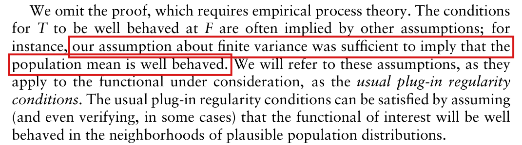
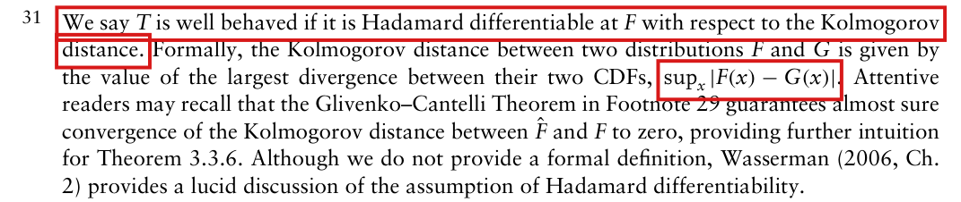
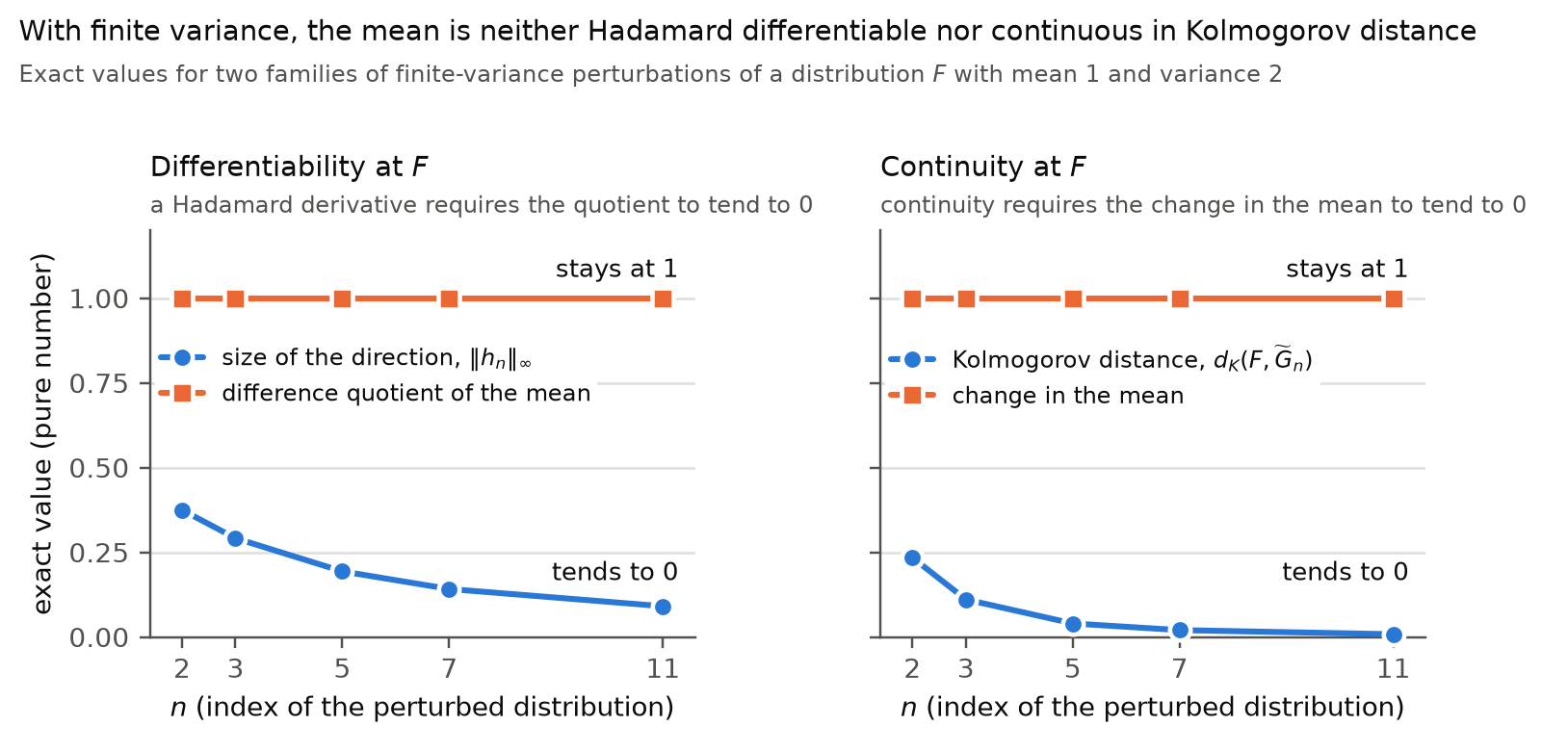
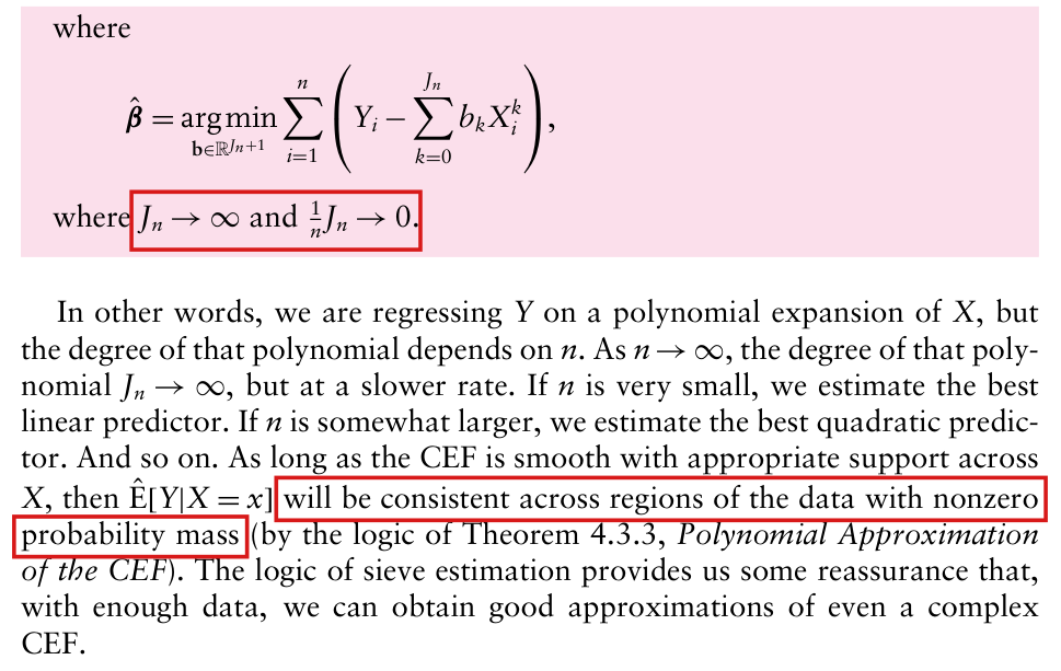
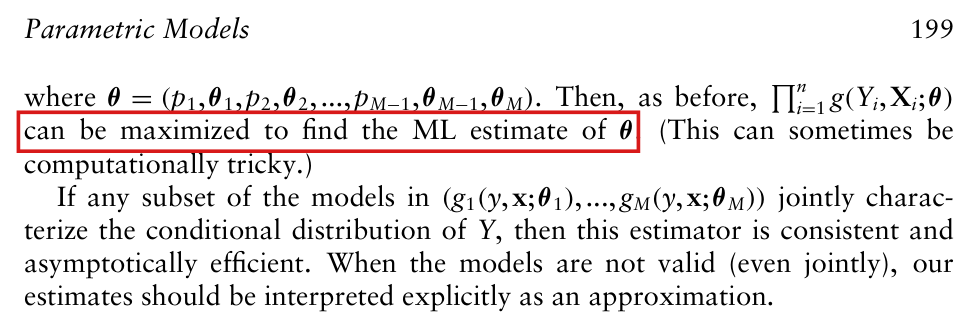
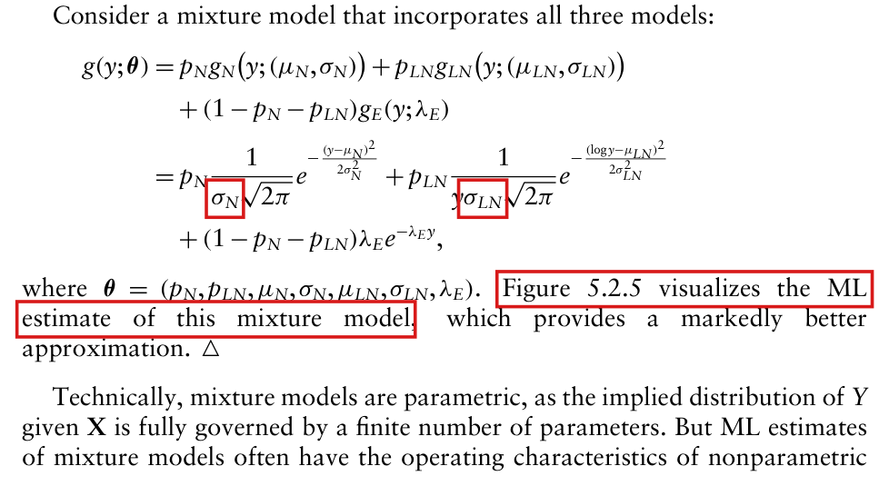
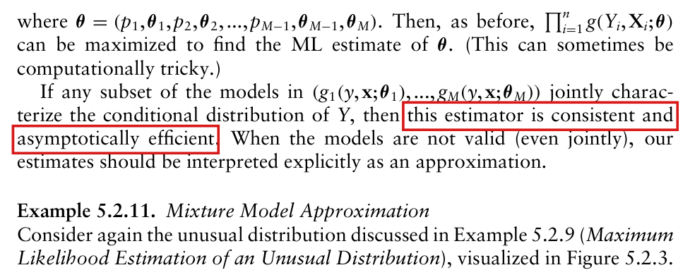
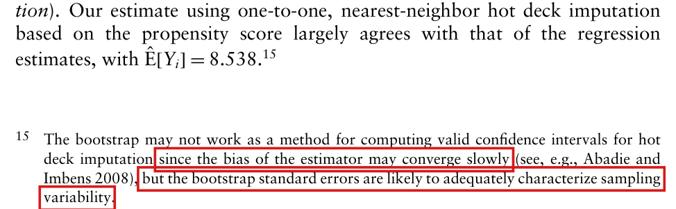
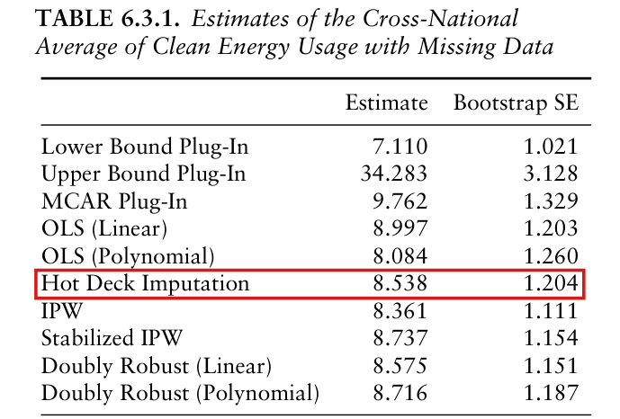
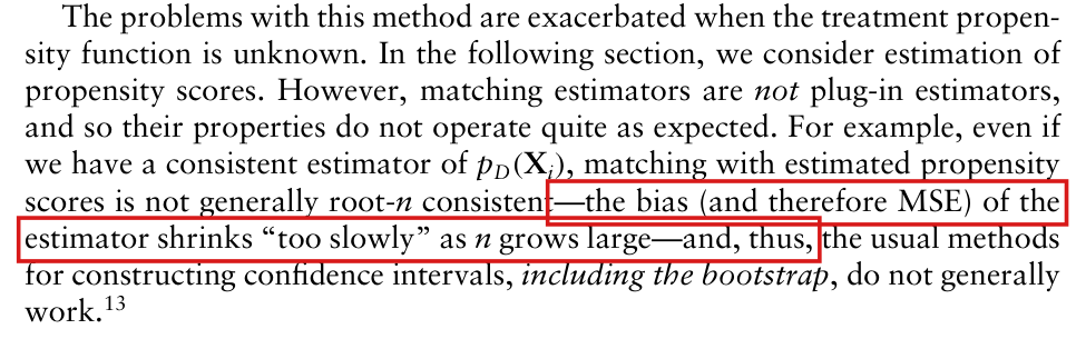

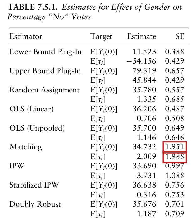
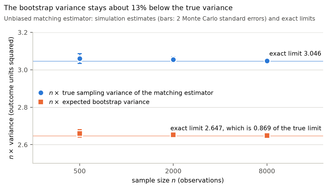
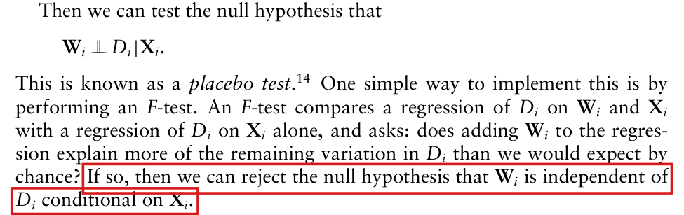
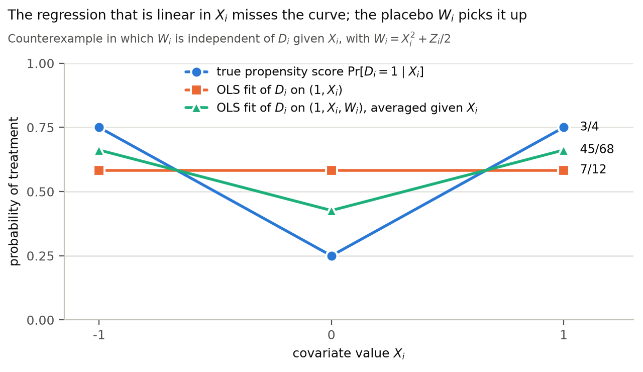
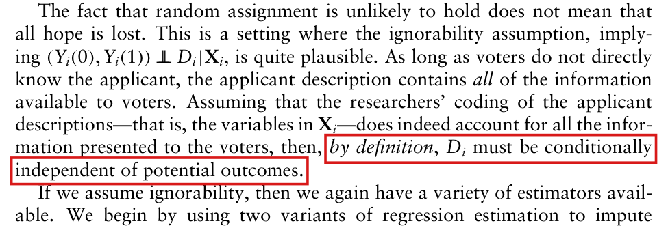
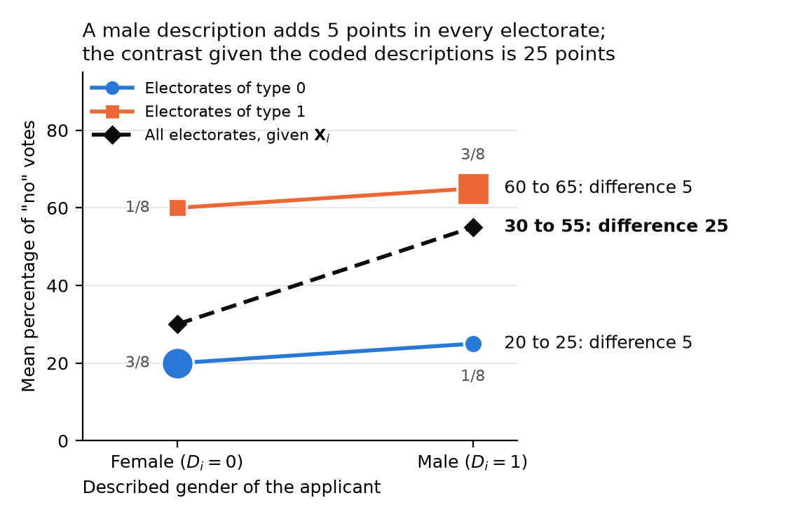




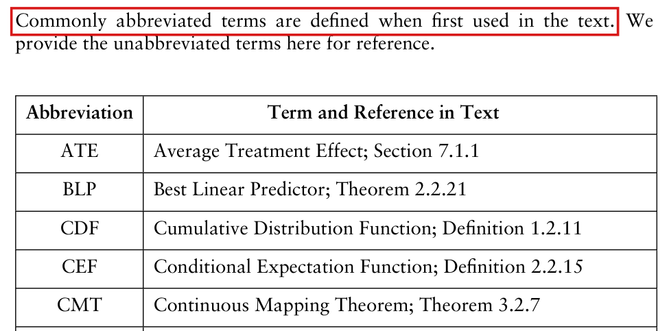
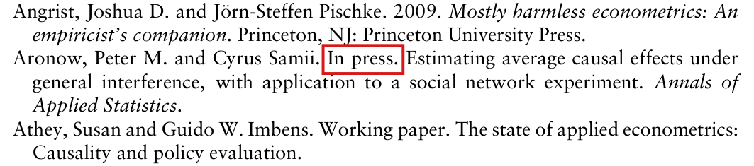


















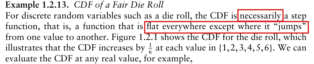

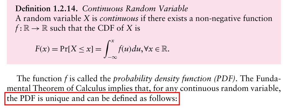
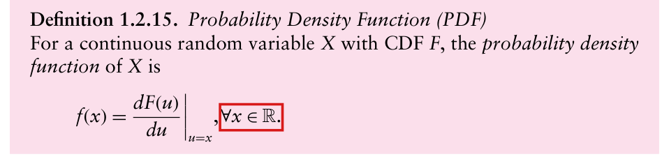
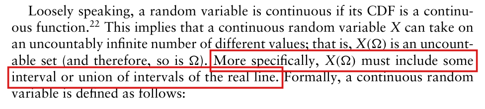
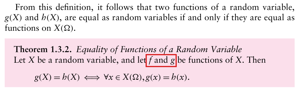






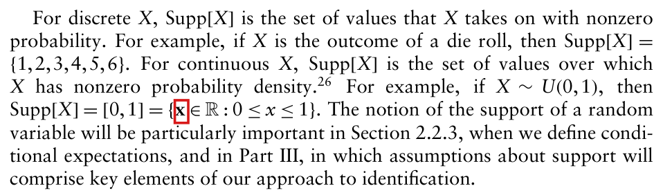
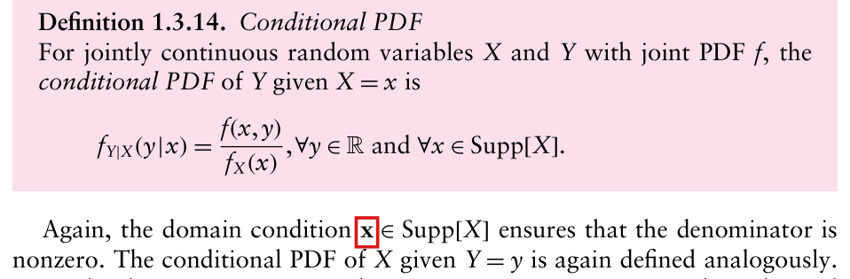
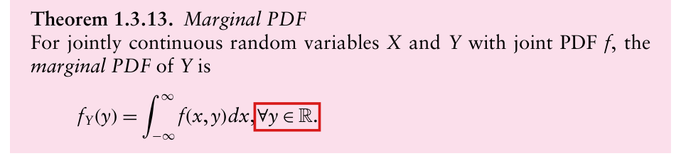
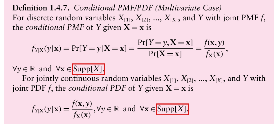
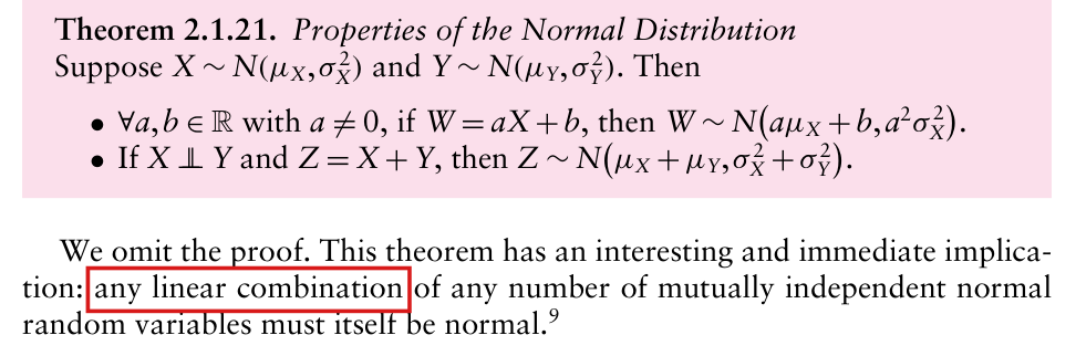
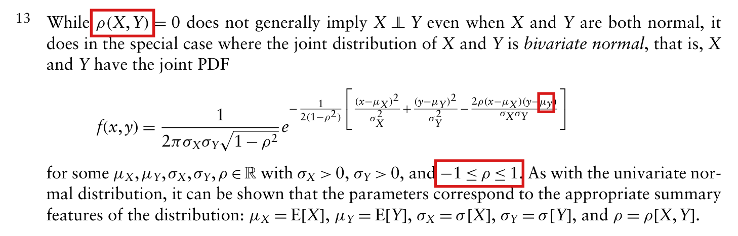
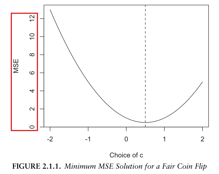
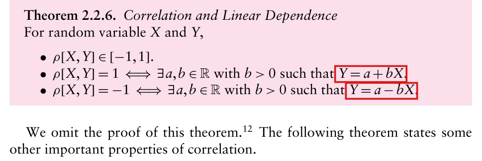
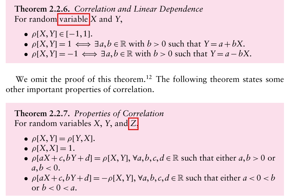
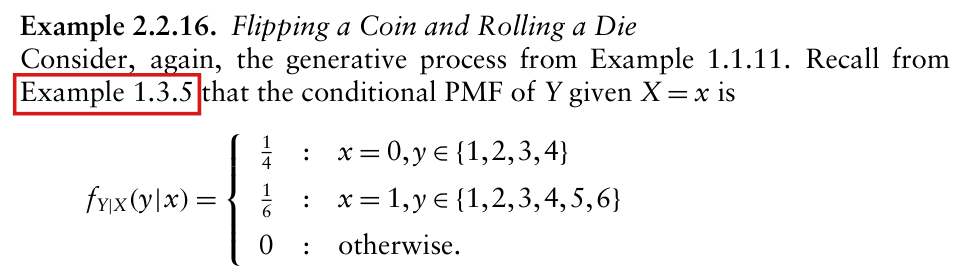
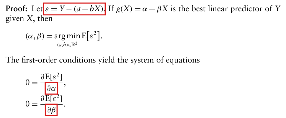
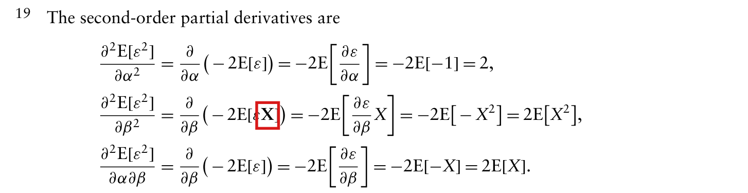

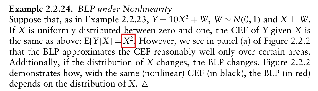

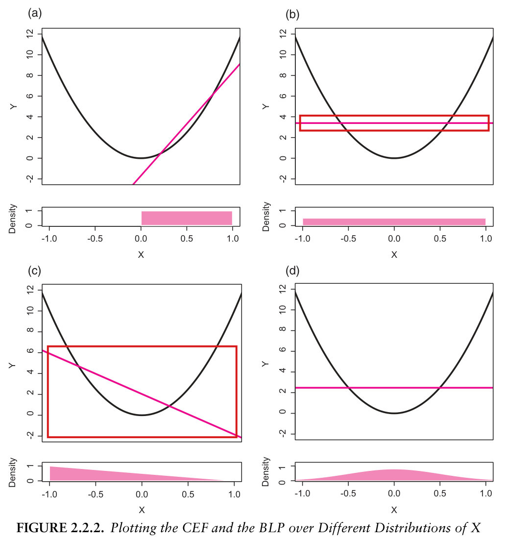
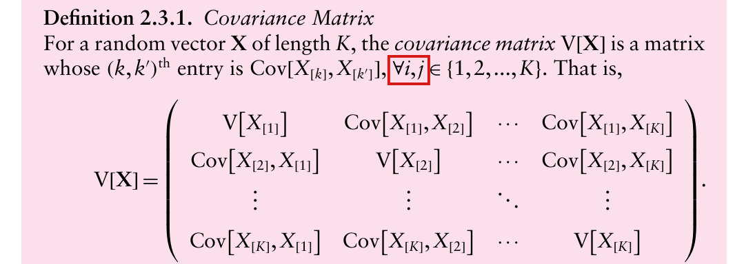
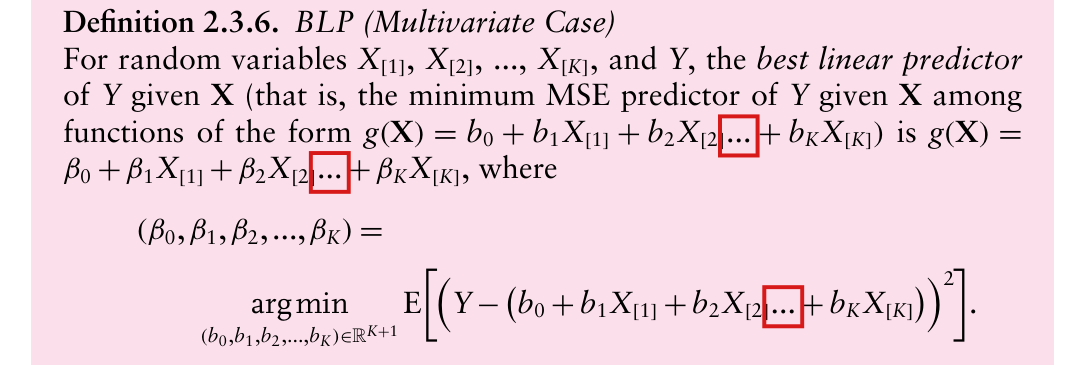

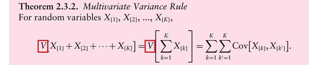


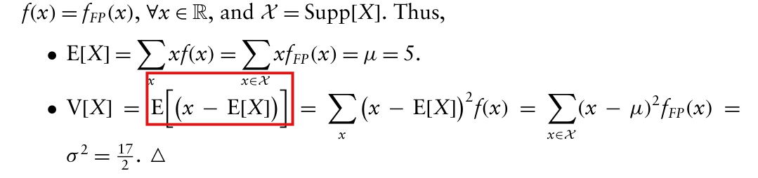
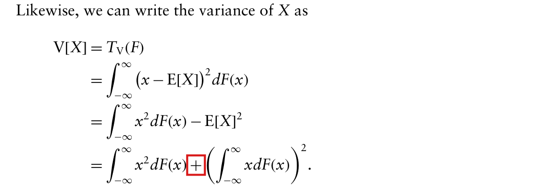
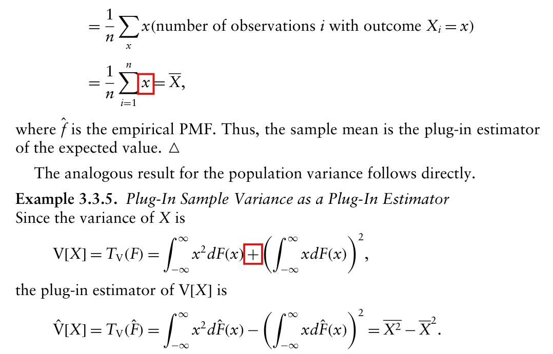
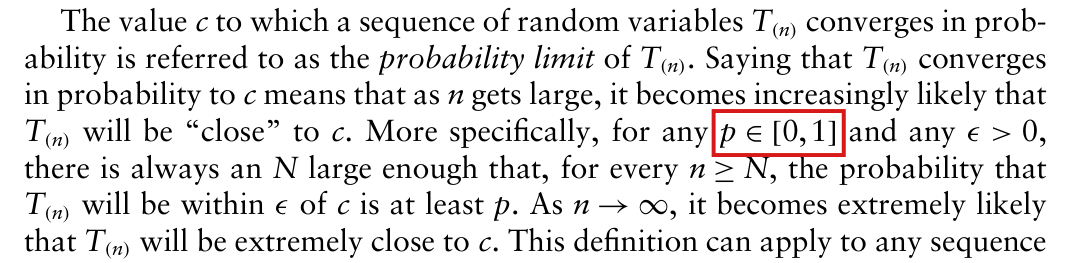


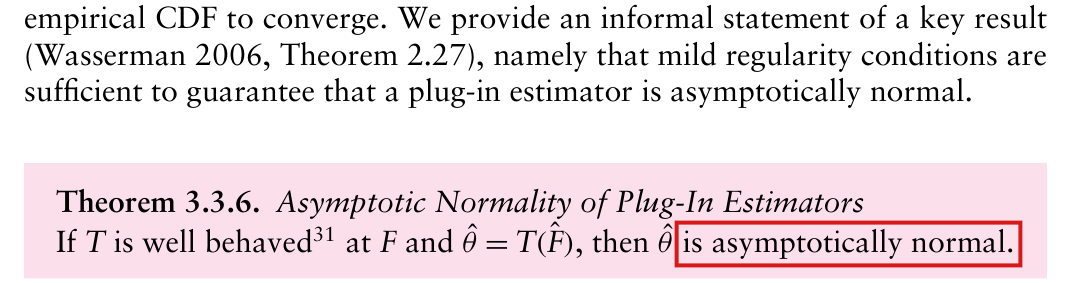
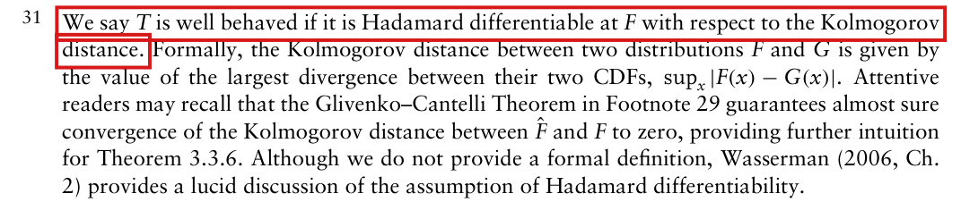

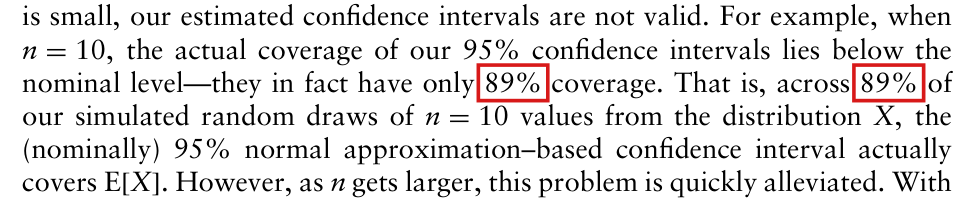
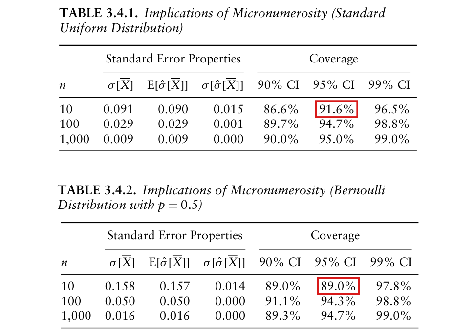
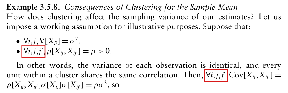
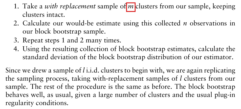



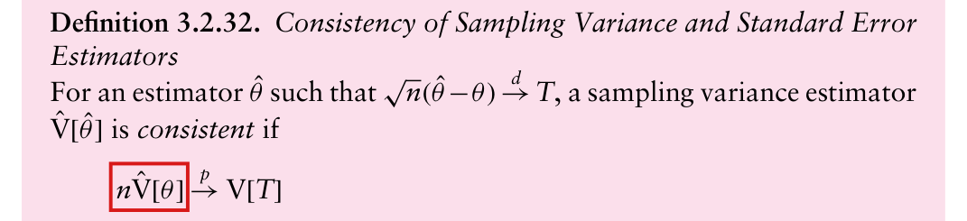










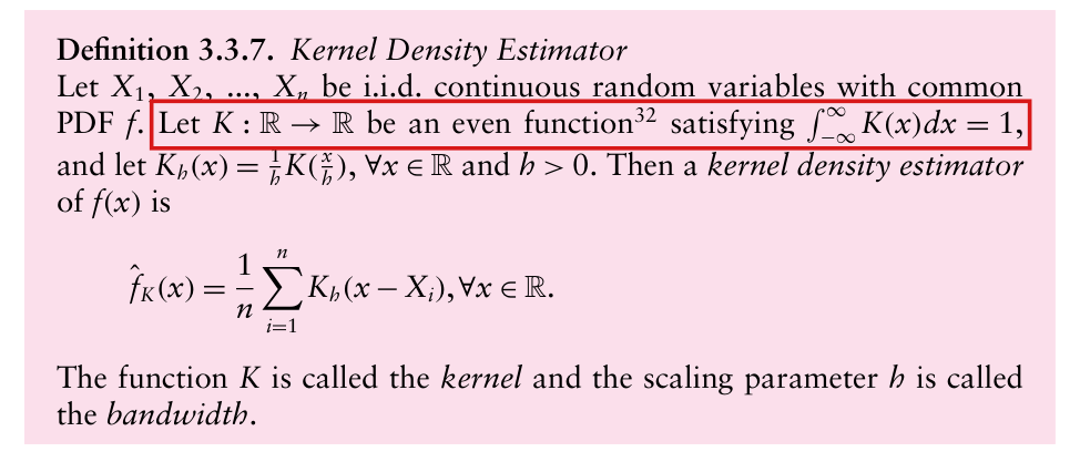
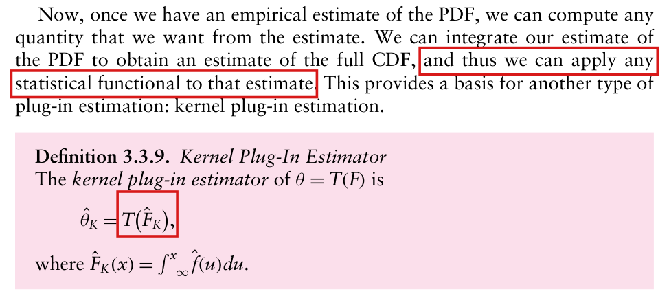
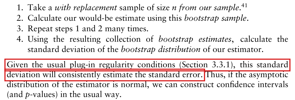



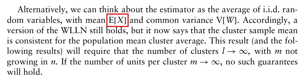
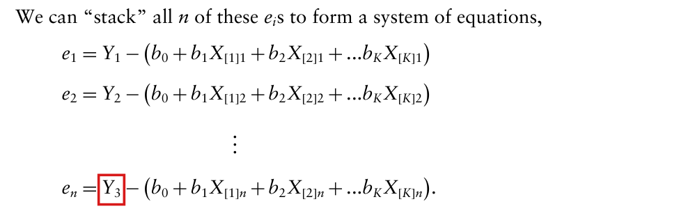
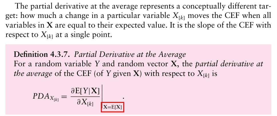
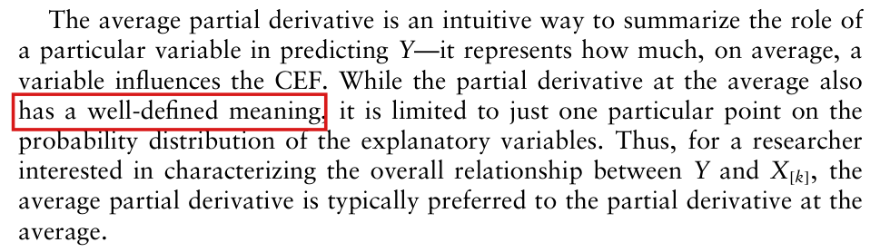
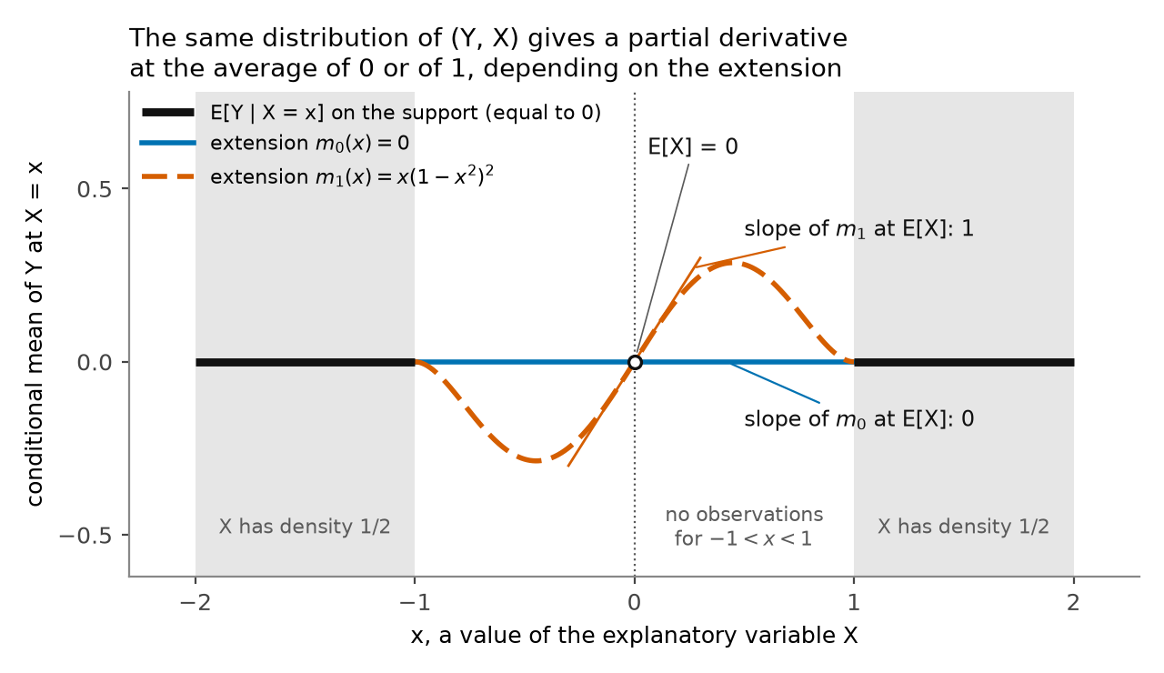
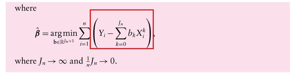

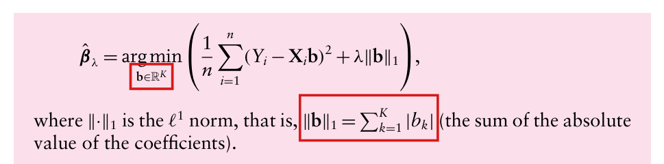
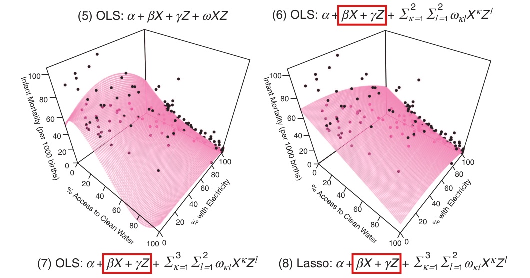

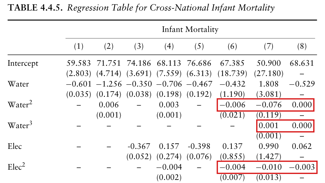
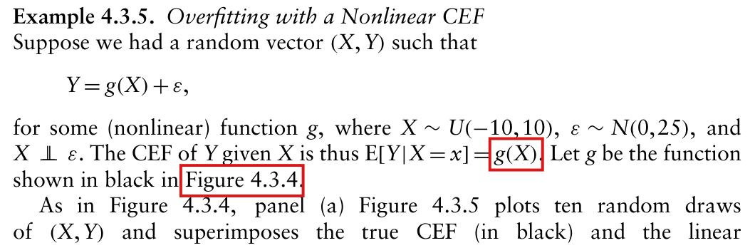
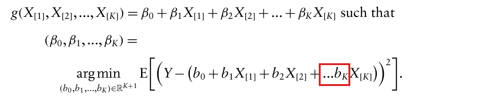
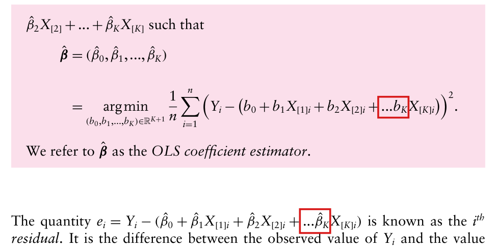
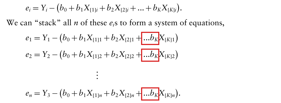


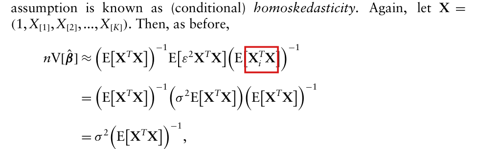
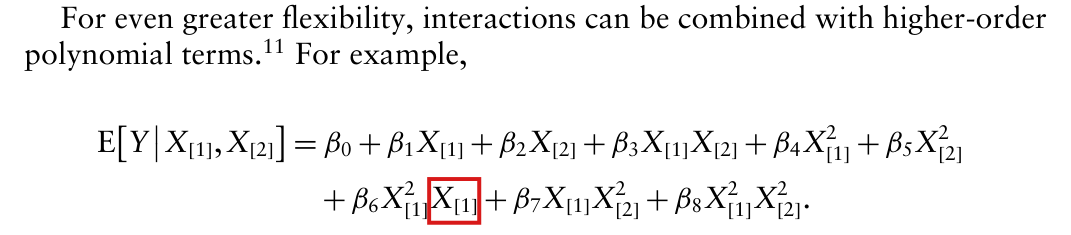

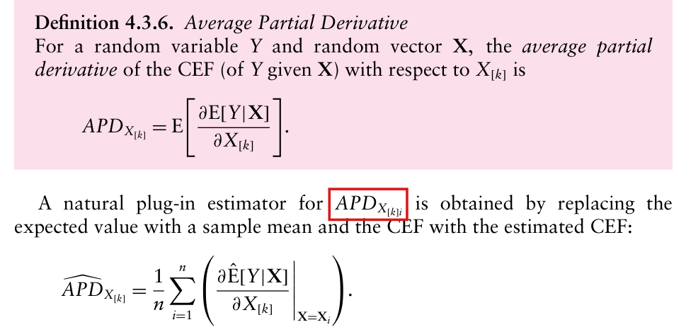
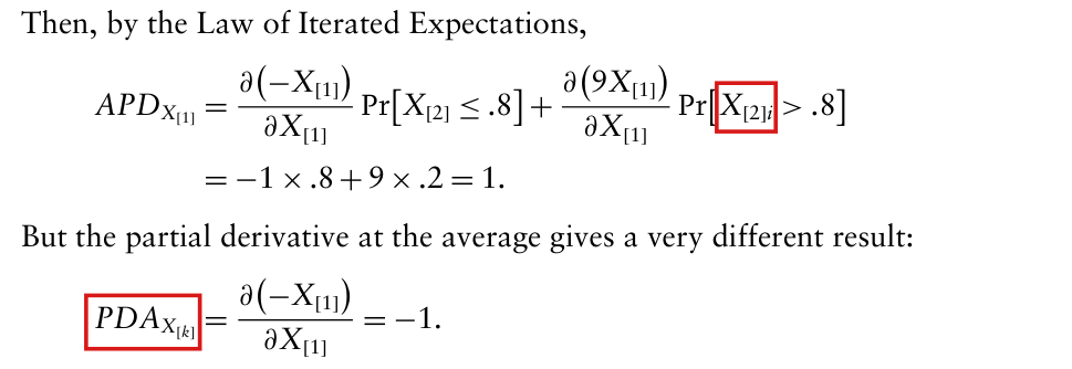
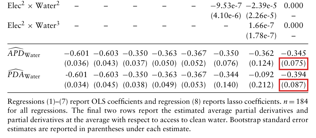
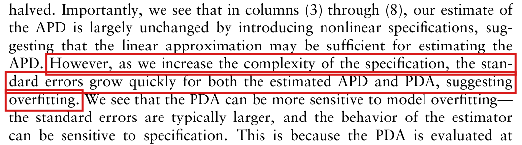

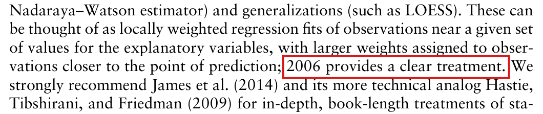
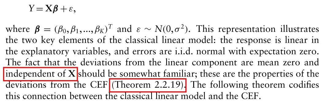

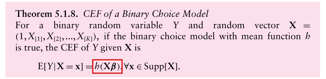
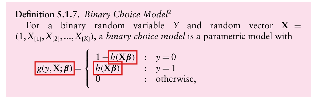
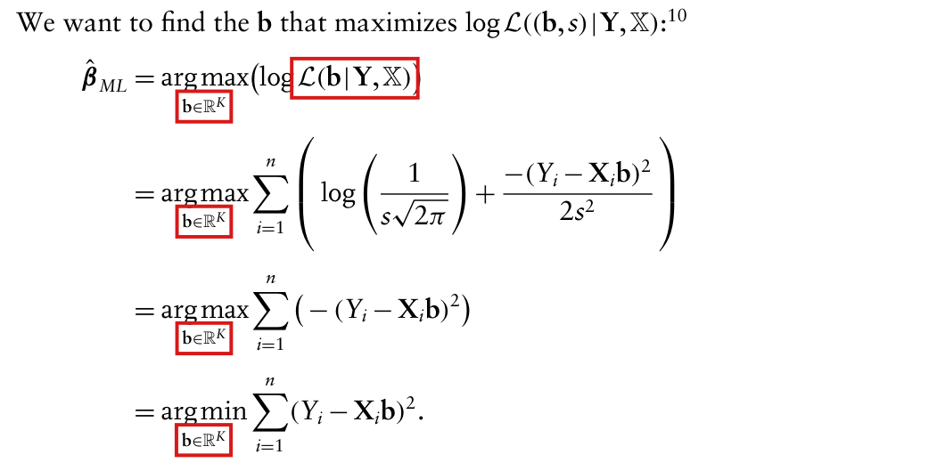



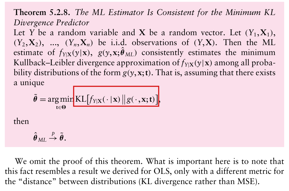
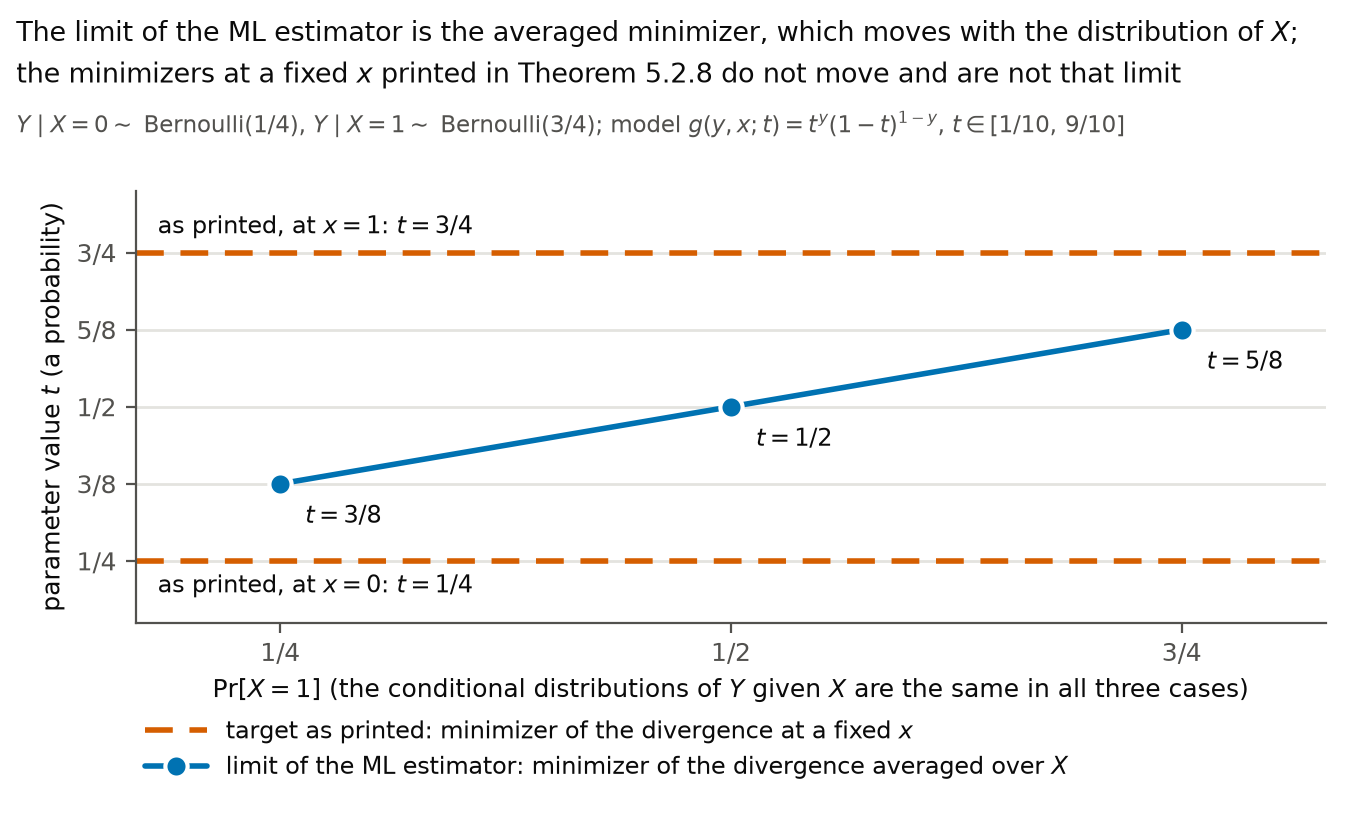
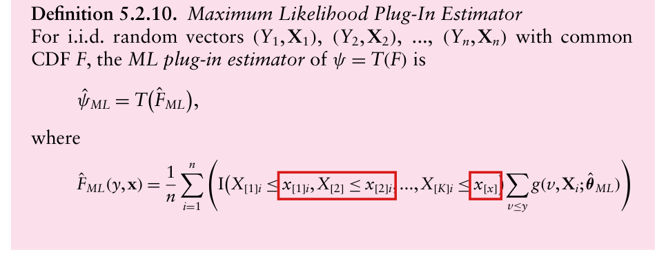
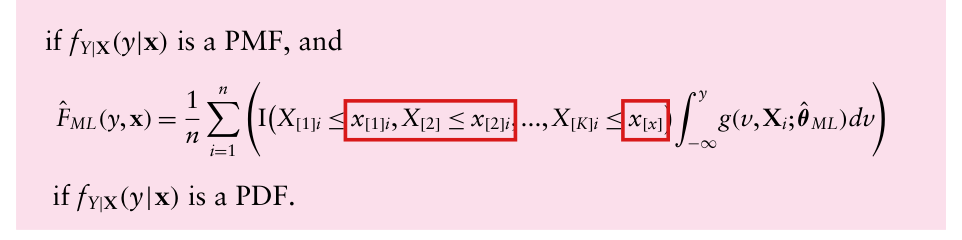

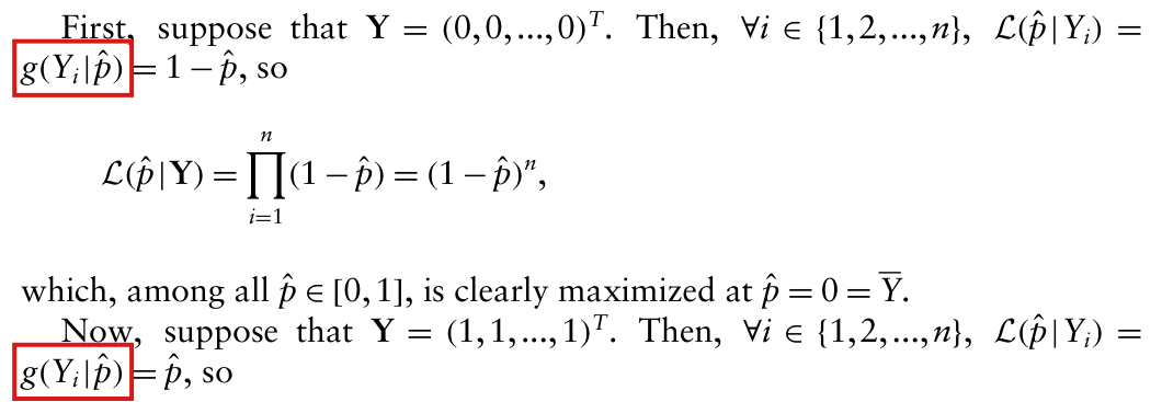
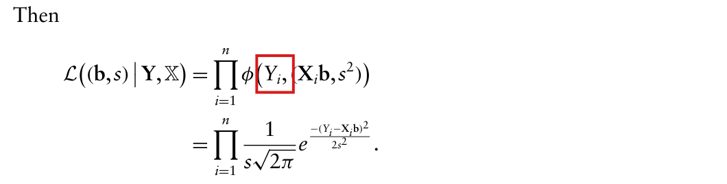
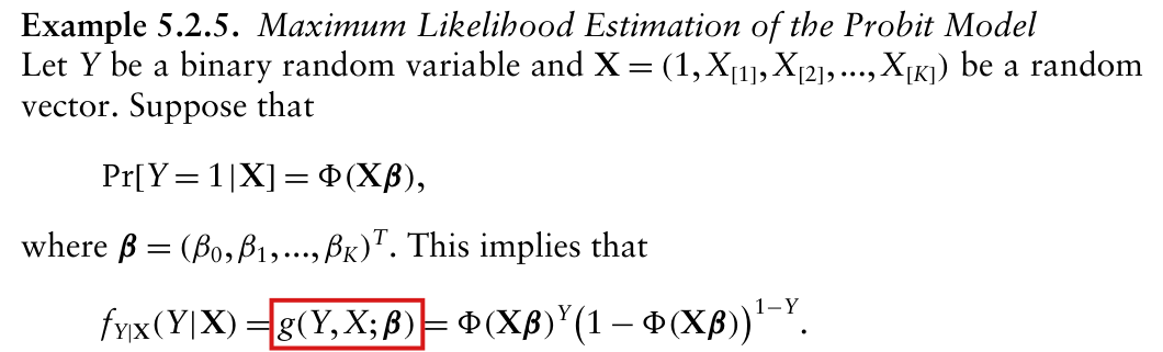

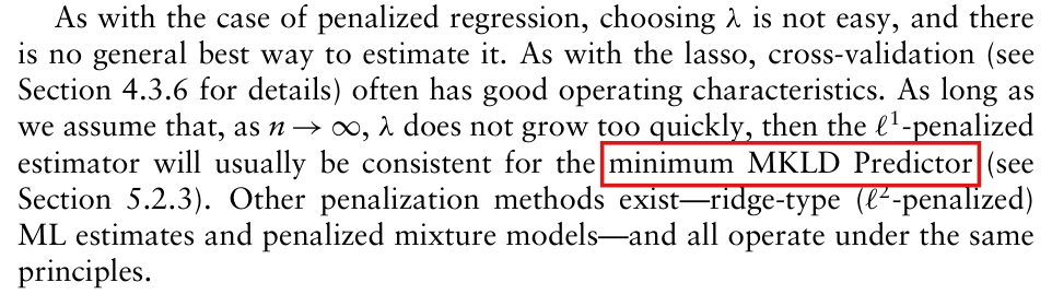
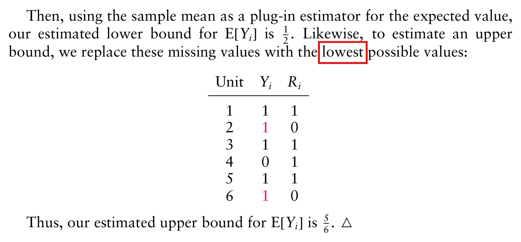

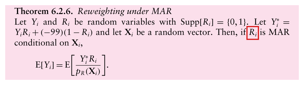
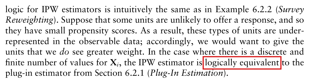
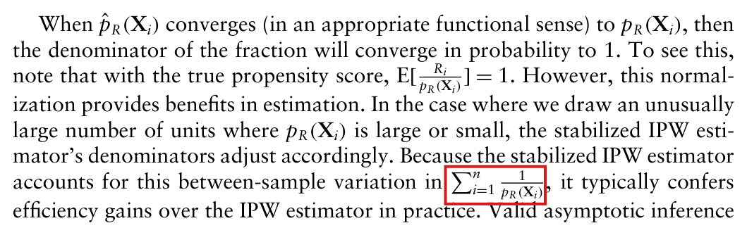
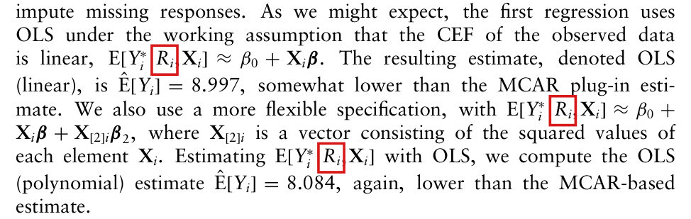


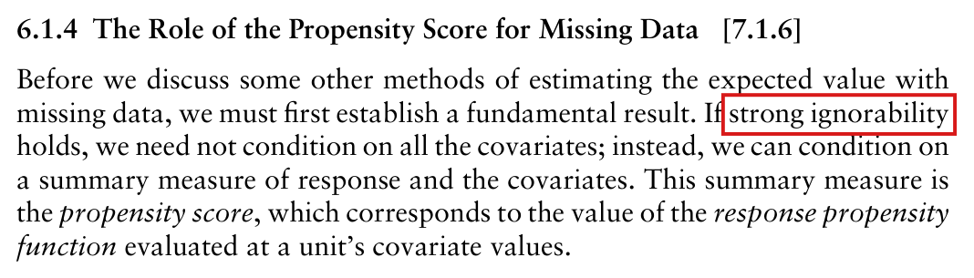


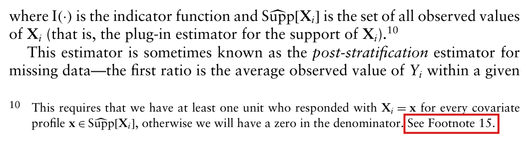

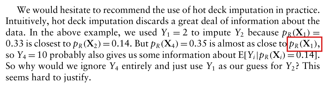






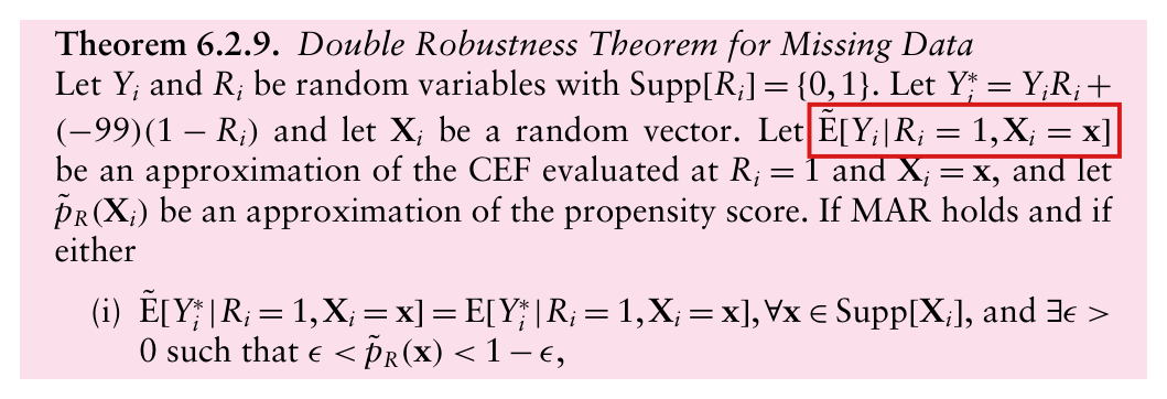
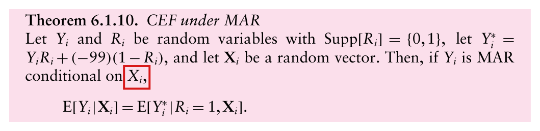




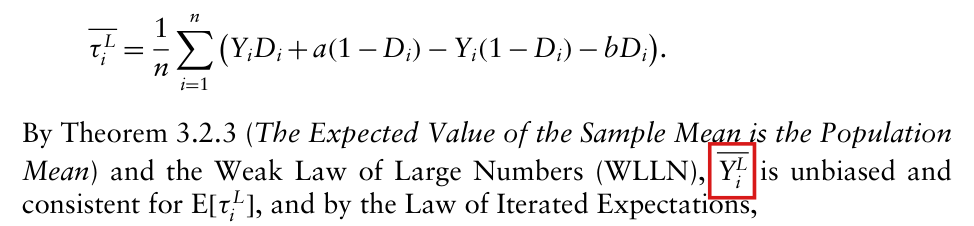

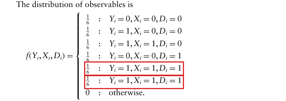
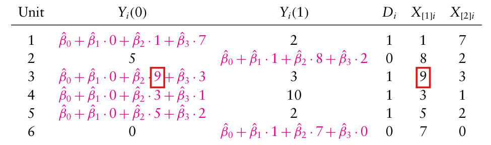
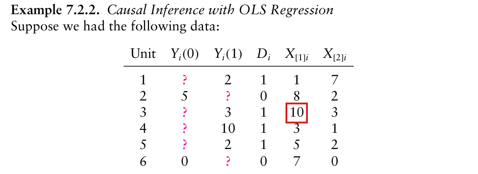
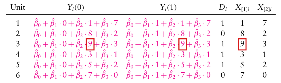
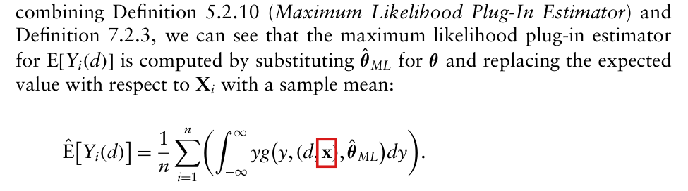

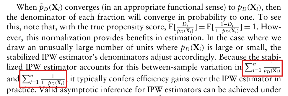
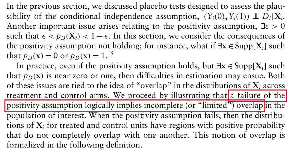
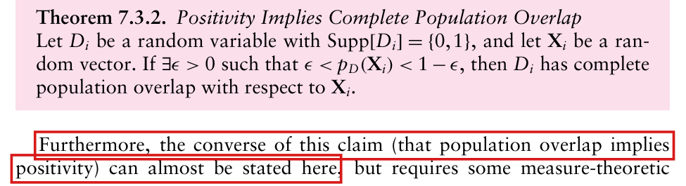
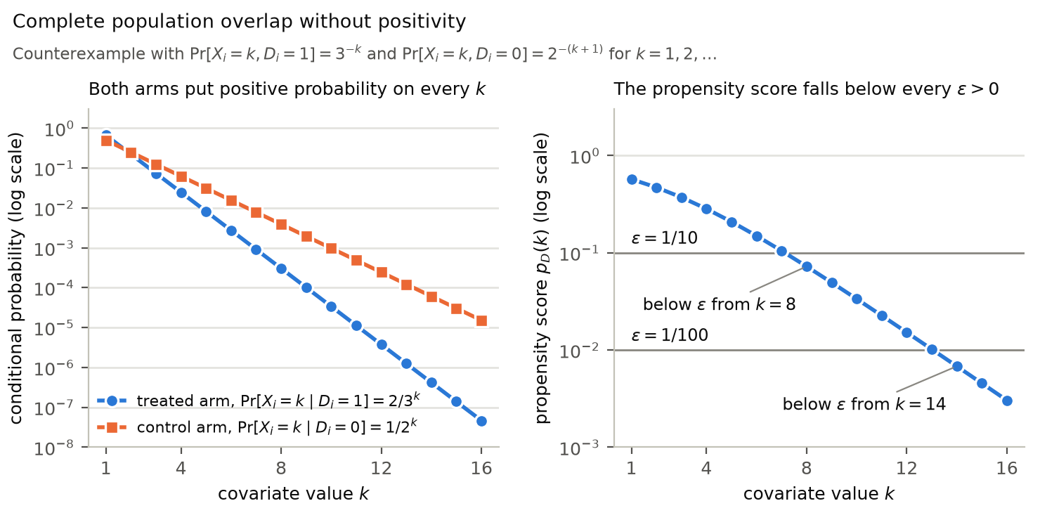



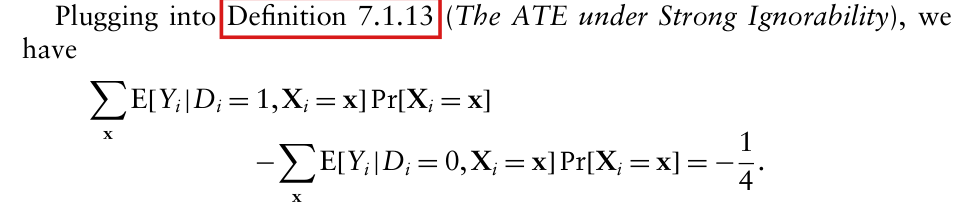
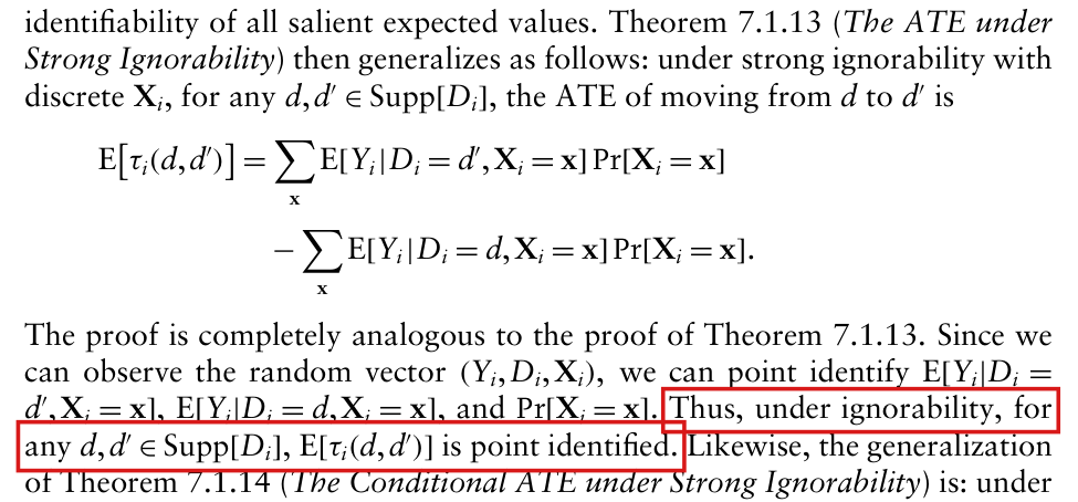


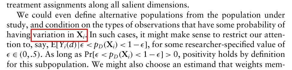


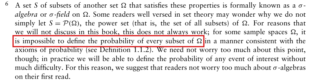

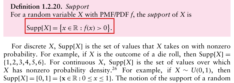
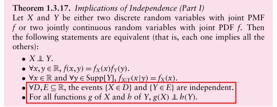
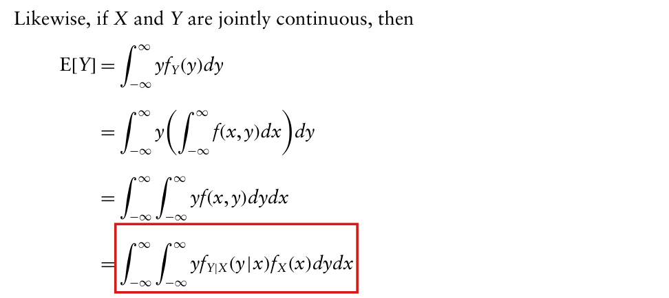
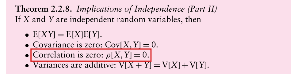
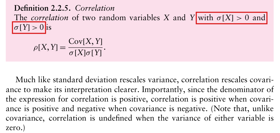
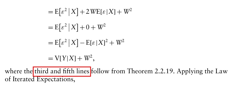
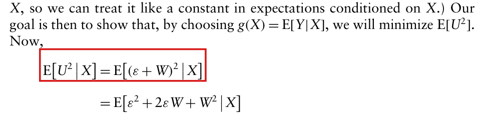
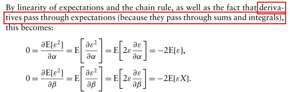
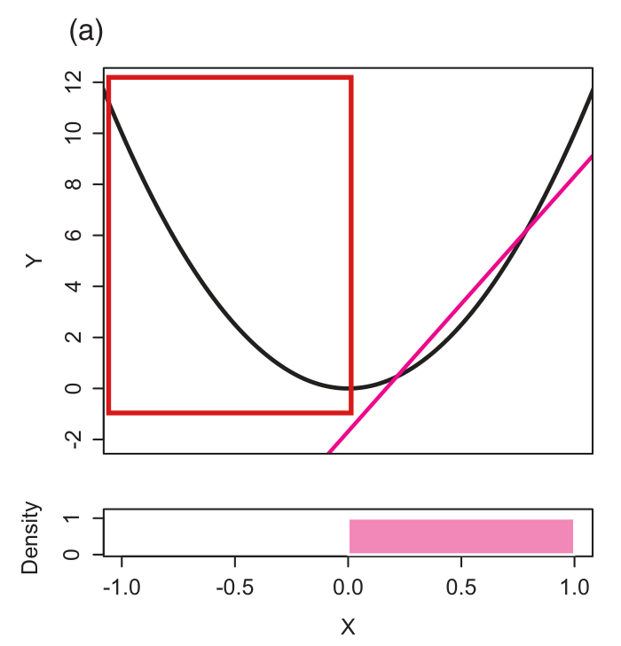
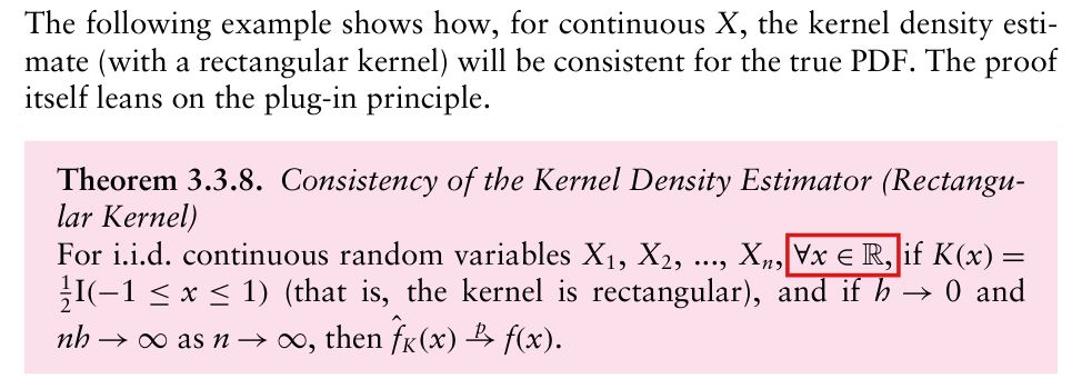

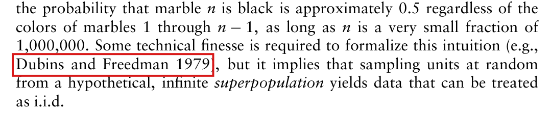
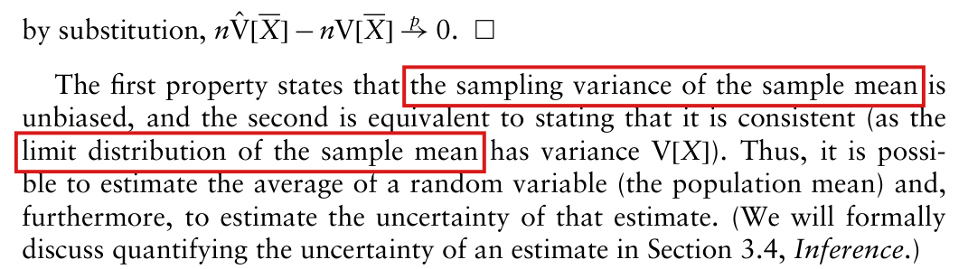
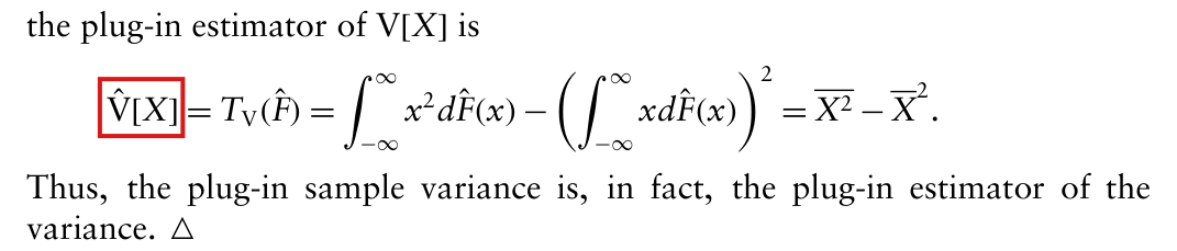

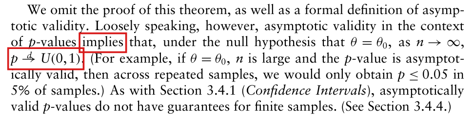

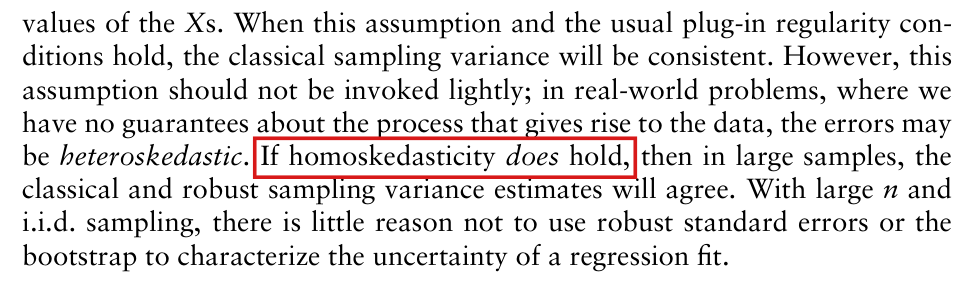
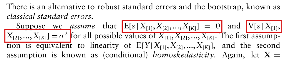

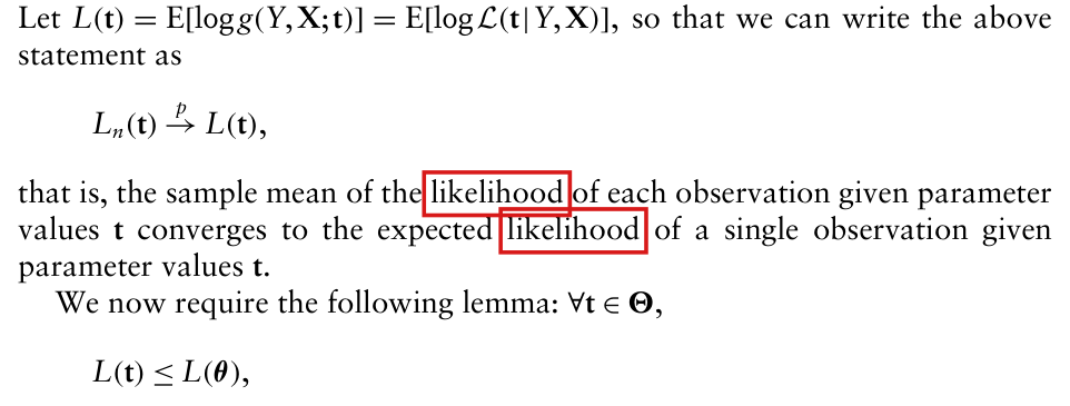
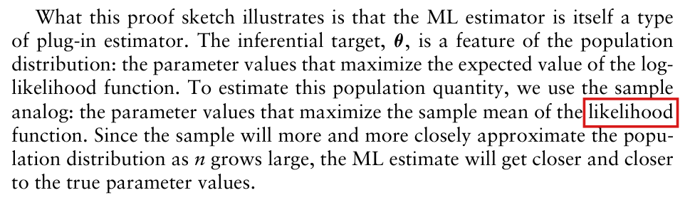
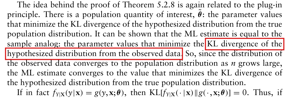
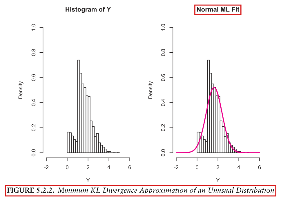
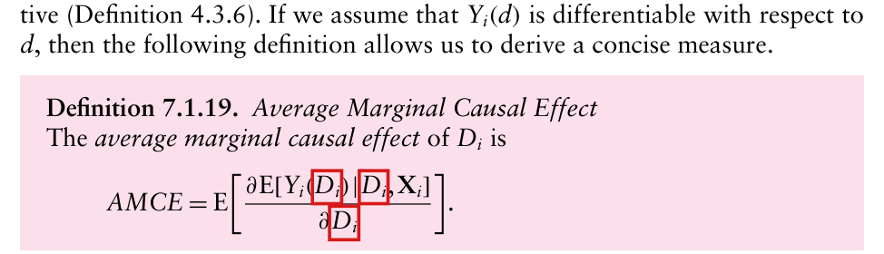
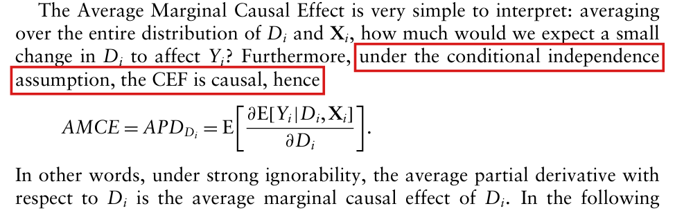

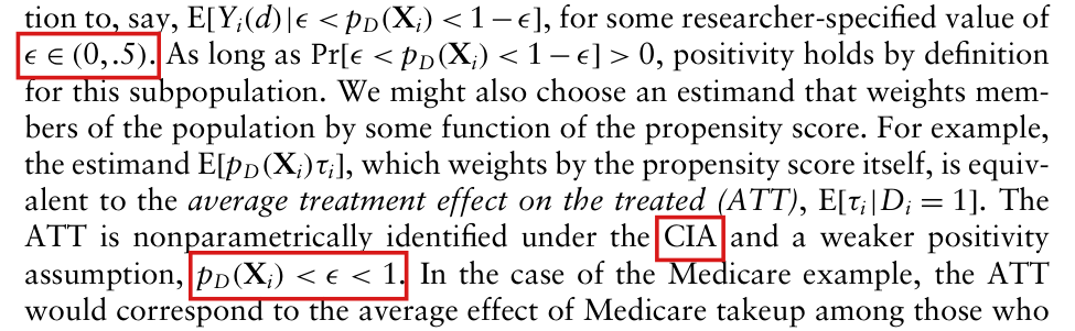
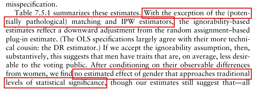
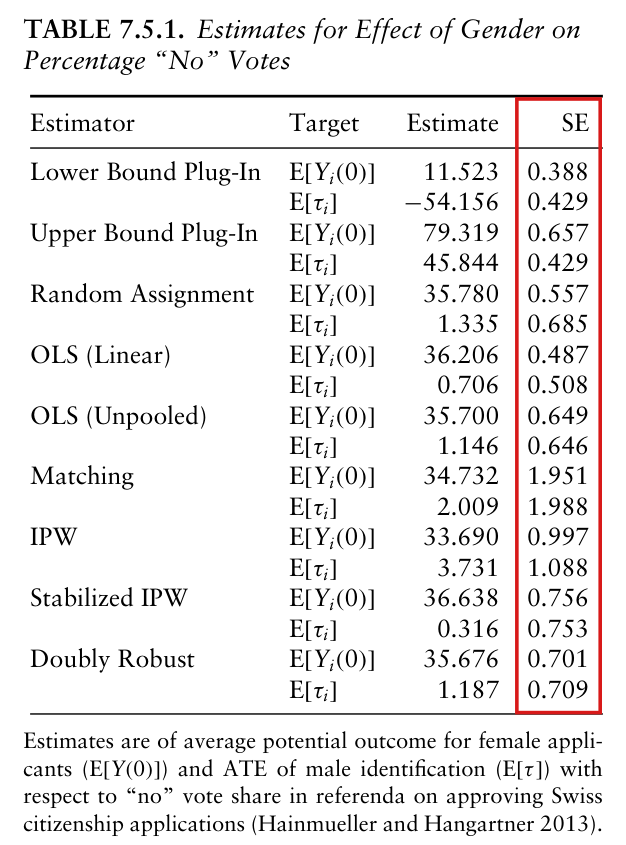
My comment and the history of this entry