Assumptions and verification
Claim revision: catalog:b20069c624c74af471c465873876c6e40e4c0d074870dab006b5353d4ed71a86
Standing assumptions: Setting, notation and standing assumptions, as printed. Every passage was read from the rendered page images (staged/pages/p-NN.png, and 220 dpi renderings of the same PDF pages for subscripts and primes). Pages are those of Econometrica, Vol. 92, No. 5 (September, 2024), 1503–1519, with the PDF page in parentheses (PDF p. 1 is the journal's cover sheet, so printed page = PDF page + 1501). Appendix A (pp. 1510–1512) and Appendix B (pp. 1512–1519) are inside the article; there is no supplement.
[Setting: Section 2, p. 1504 (PDF p. 3)] “We follow the setting of Freedman (2008a), Lin (2013), Abadie, Athey, Imbens, and Wooldridge (2020), and Lei and Ding (2021), which assume a Neyman model with covariates (Splawa-Neyman, Dabrowska, and Speed (1923)). There are $n$ subjects indexed by $i = 1, \ldots, n$. For each subject, we observe an outcome $Y_i$ and a column vector of covariates $x_i = (x_{i1}, x_{i2}, \ldots, x_{id})' \in \mathbb{R}^d$. Each subject has two potential outcomes $y_i(1)$ and $y_i(0)$. We observe $Y_i = y_i(1)$ if subject $i$ is assigned to the treatment arm $T$, and $Y_i = y_i(0)$ if subject $i$ is assigned to the control arm $C$. Let $D_i$ be a binary variable, where $D_i = 1$ indicates that subject $i$ is assigned to the treatment arm.”
[Design: p. 1505 (PDF p. 4)] “The experiment is assumed to be completely randomized, where $n_T$ out of $n$ subjects are randomly assigned to the treatment arm $T$ and the remaining $n_C = n - n_T$ subjects are assigned to the control arm $C$. Random assignment is the sole source of randomness in our statistical analysis. The potential outcomes and covariates are considered fixed, and the bias of an estimator is assessed relative to the randomization distribution of the estimator. We do not assume the existence of a superpopulation: the $n$ subjects are the population of interest.”
[Notation: p. 1505 (PDF p. 4)] “We define $[T]$ as the set of subjects chosen for the treatment arm, given by $\{i \mid D_i = 1\}$, and similarly $[C]$ as the set of subjects chosen for the control arm, given by $\{i \mid D_i = 0\}$. For a possibly matrix-valued variable $a_i$, we use the notation $\bar a = \frac1n\sum_{i=1}^n a_i$ to represent the population average, $\bar a_T = \frac{1}{n_T}\sum_{i\in[T]}a_i$ to denote the treatment group average, and $\bar a_C = \frac{1}{n_C}\sum_{i\in[C]}a_i$ to denote the control group average. The average treatment effect (ATE) can be expressed in this notation as $\mathrm{ATE} = \overline{y(1)} - \overline{y(0)}$, and the difference-in-means estimator is given by $\overline{Y}_T - \overline{Y}_C$. Similarly, we can write $\frac1n\sum_{i=1}^n x_ix_i' = \overline{xx'}$ for $x_i \in \mathbb{R}^d$ and $\frac1n\sum_{i=1}^n y_i(1)x_i = \overline{y(1)x}$ for $y_i(1) \in \mathbb{R}$ and $x_i \in \mathbb{R}^d$.”
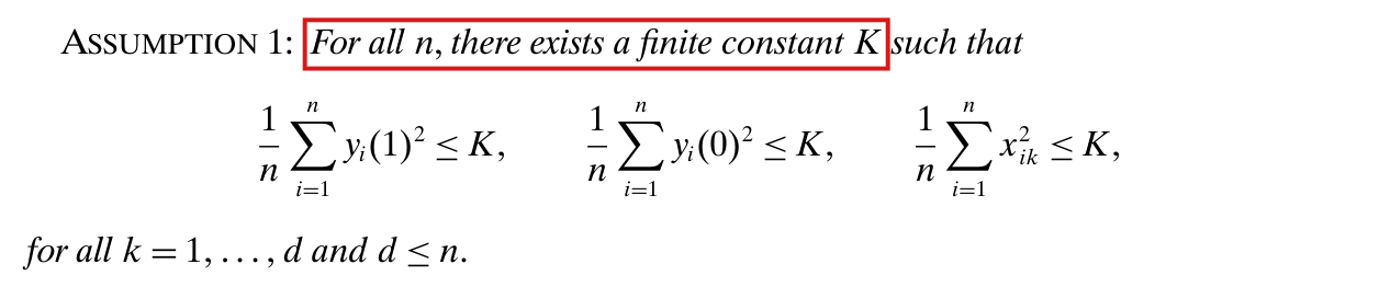
[Assumptions: p. 1505 (PDF p. 4)] “We make the following assumptions throughout the paper, which are standard in the literature.” ASSUMPTION 1: “For all $n$, there exists a finite constant $K$ such that $\frac1n\sum_{i=1}^n y_i(1)^2 \le K$, $\frac1n\sum_{i=1}^n y_i(0)^2 \le K$, $\frac1n\sum_{i=1}^n x_{ik}^2 \le K$, for all $k = 1, \ldots, d$ and $d \le n$.” ASSUMPTION 2: “For all $n$ large enough, (1) $\bar x = 0$, and (2) $\overline{xx'} = I_d$, the $d \times d$ identity matrix.” ASSUMPTION 3: “Let $p_{T,n} = \frac{n_T}{n}$ and $p_{C,n} = \frac{n-n_T}{n}$ denote the inclusion probabilities into the treatment arm $T$ and control arm $C$, respectively. There exist positive constants $p_{\min}$ and $p_{\max}$ such that $0 < p_{\min} < p_{\max} < 1$ and $p_{\min} < p_{T,n} < p_{\max}$ for all $n$.” Then: “We shall hereafter omit the $n$ subscript in $p_{T,n}$ and $p_{C,n}$, and write $p_T$ and $p_C$ unless otherwise noted.”
[The two estimators: pp. 1505–1506 (PDF pp. 4–5)] “The first estimator results from a OLS regression: $Y_i \sim \alpha + \tau D_i + x_i'\beta$, (1) where one regresses observed outcome $Y_i$ on the treatment indicator $D_i$ and covariates $x_i$. We denote the OLS estimators for this case as $(\widehat\alpha, \widehat\tau, \widehat\beta)$. The estimator $\widehat\tau$ is hereafter referred to as the noninteracted ATE estimator. The second estimator results from an interacted OLS regression where researchers expand the covariates by including terms interacting the treatment indicator and covariates: $Y_i \sim \alpha_I + \tau_ID_i + x_i'\beta_{I,C} + D_ix_i'\beta_{I,T}$. (2) We denote the OLS estimators for the interacted case as $(\widehat\alpha_I, \widehat\tau_I, \widehat\beta_{I,C}, \widehat\beta_{I,T})$. The estimator $\widehat\tau_I$ is hereafter referred to as the interacted ATE estimator.”
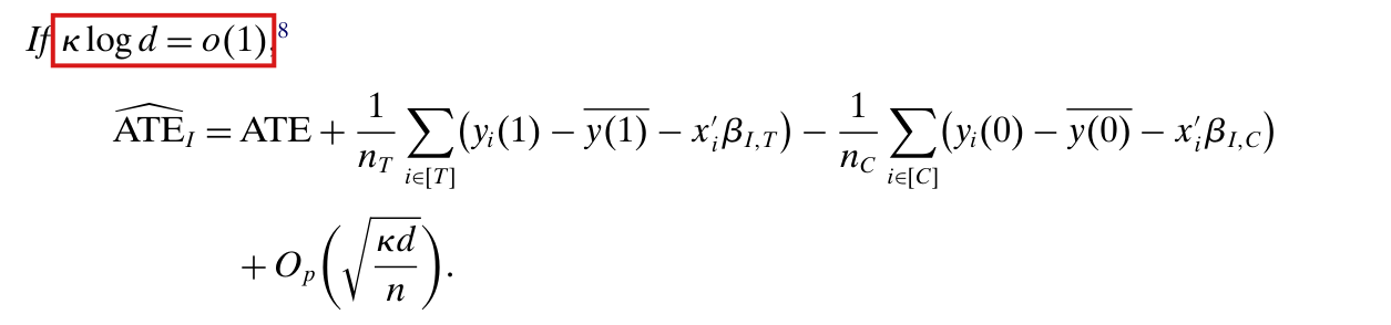
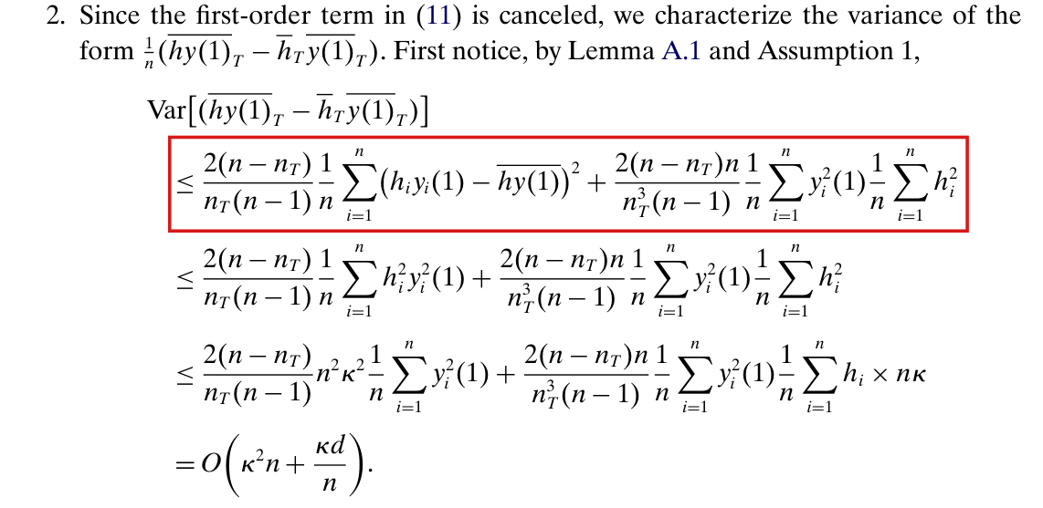
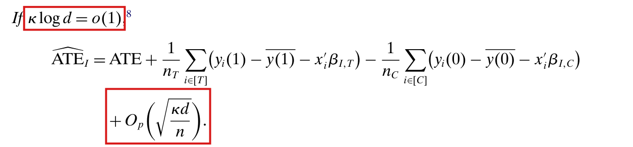
[Section 3 objects: p. 1506 (PDF p. 5)] “As shown in Lin (2013), the noninteracted ATE estimator can be written as $\widehat{\mathrm{ATE}} = \overline{y(1)}_T - \overline{y(0)}_C - (\bar x_T'\widehat\beta - \bar x_C'\widehat\beta)$, (3) where $\widehat\beta$ is the OLS coefficient estimators for the covariates.” “The coefficient estimators $\widehat\beta$ can be algebraically written as $\widehat\beta = \widehat L^{-1}\widehat N$, where $\widehat L = I_d - p_T\bar x_T\bar x_T' - p_C\bar x_C\bar x_C'$ and $\widehat N = p_T(\overline{y(1)x}_T - \overline{y(1)}_T\bar x_T) + p_C(\overline{y(0)x}_C - \overline{y(0)}_C\bar x_C)$ by an application of the Frisch–Waugh–Lovell theorem.” “The OLS coefficient estimators can be thought of as estimating the (finite) population coefficients $\beta^* = L^{-1}N$, where $L = I_d$ and $N = p_T\overline{y(1)x} + p_C\overline{y(0)x}$.” Footnote 4: “Note we shall hereafter assume for simplicity that all design matrices, $\widehat L$, are invertible. In the case of noninvertible design matrices, our debiased procedure will still work after choosing an arbitrary generalized inverse matrix and computing the ATE estimators accordingly.” “Let $y_i^*(1)$ and $y_i^*(0)$ be the centered potential outcomes, that is, $y_i^*(1) = y_i(1) - \overline{y(1)}$ and $y_i^*(0) = y_i(0) - \overline{y(0)}$. Denote the (rescaled) leverage of the $i$th subject as $h_i = \|x_i\|_2^2$. As in Lei and Ding (2021), we define the maximum leverage as $\kappa = \max_{i=1,\ldots,n}\frac{h_i}{n} = \max_{i=1,\ldots,n}\frac{\|x_i\|_2^2}{n}$. (4)”
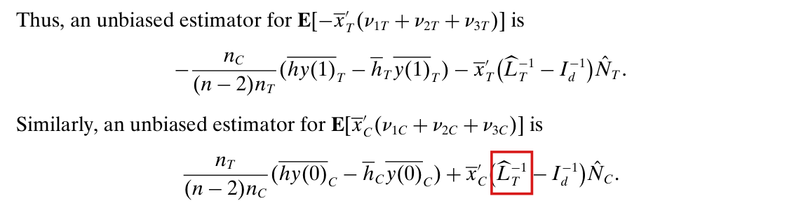
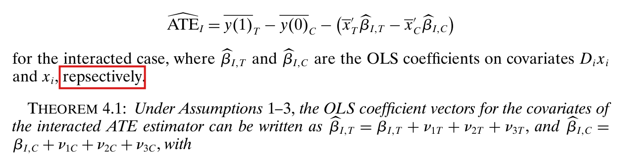
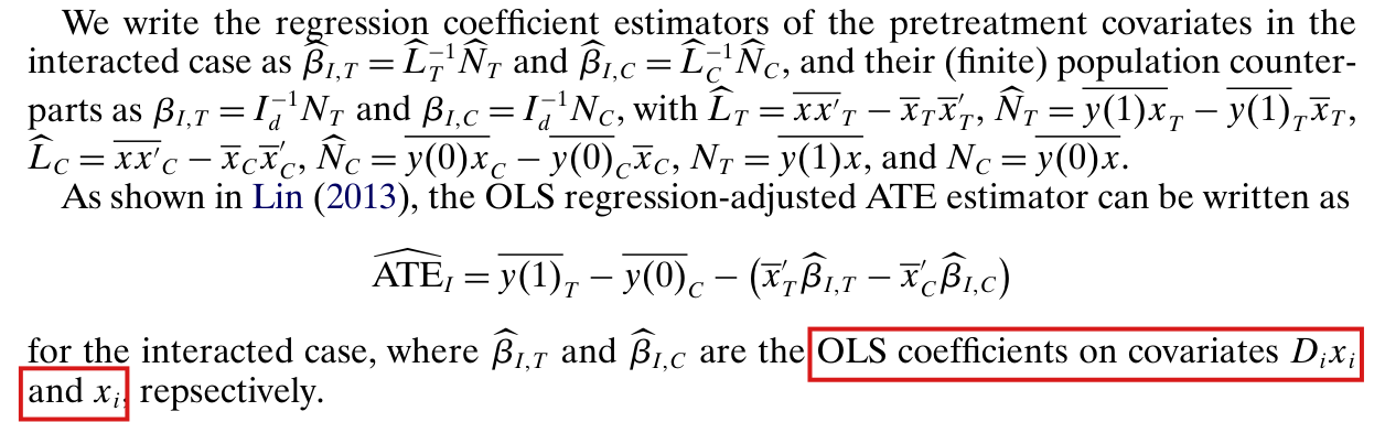
[Section 4 objects: p. 1509 (PDF p. 8)] “We write the regression coefficient estimators of the pretreatment covariates in the interacted case as $\widehat\beta_{I,T} = \widehat L_T^{-1}\widehat N_T$ and $\widehat\beta_{I,C} = \widehat L_C^{-1}\widehat N_C$, and their (finite) population counterparts as $\beta_{I,T} = I_d^{-1}N_T$ and $\beta_{I,C} = I_d^{-1}N_C$, with $\widehat L_T = \overline{xx'}_T - \bar x_T\bar x_T'$, $\widehat N_T = \overline{y(1)x}_T - \overline{y(1)}_T\bar x_T$, $\widehat L_C = \overline{xx'}_C - \bar x_C\bar x_C'$, $\widehat N_C = \overline{y(0)x}_C - \overline{y(0)}_C\bar x_C$, $N_T = \overline{y(1)x}$, and $N_C = \overline{y(0)x}$. As shown in Lin (2013), the OLS regression-adjusted ATE estimator can be written as $\widehat{\mathrm{ATE}}_I = \overline{y(1)}_T - \overline{y(0)}_C - (\bar x_T'\widehat\beta_{I,T} - \bar x_C'\widehat\beta_{I,C})$ for the interacted case, where $\widehat\beta_{I,T}$ and $\widehat\beta_{I,C}$ are the OLS coefficients on covariates $D_ix_i$ and $x_i$, repsectively.”
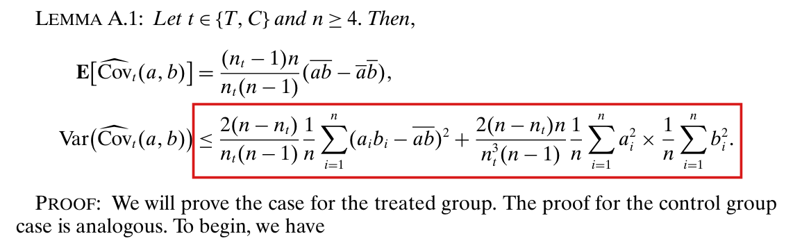
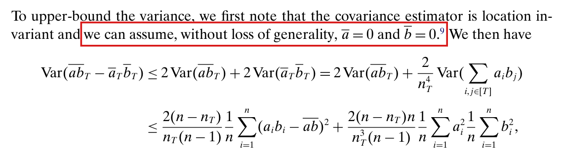
[Appendix A objects: p. 1510 (PDF p. 9)] “We define the following three constants: $N_{\mathrm{TTT}} = \frac{(n-n_T)(n-2n_T)}{(n-1)(n-2)n_T^2} = \frac{n_C(n_C-n_T)}{(n-1)(n-2)n_T^2}$, $N_{\mathrm{CCC}} = \frac{(n-n_C)(n-2n_C)}{(n-1)(n-2)n_C^2} = \frac{n_T(n_T-n_C)}{(n-1)(n-2)n_C^2}$, $N_{\mathrm{TTC}} = -\frac{(n-2n_T)}{(n-1)(n-2)n_T} = \frac{n_T-n_C}{(n-1)(n-2)n_T}$.” “Let $a = (a_1, \ldots, a_n) \in \mathbb{R}^n$ and $b = (b_1, \ldots, b_n) \in \mathbb{R}^n$ be arbitrary $n$-vectors with fixed elements. We define the covariance estimator for the treated group as $\widehat{\mathrm{Cov}}_T(a,b) = \overline{ab}_T - \bar a_T\bar b_T$, and similarly for the control group as $\widehat{\mathrm{Cov}}_C(a,b) = \overline{ab}_C - \bar a_C\bar b_C$.”
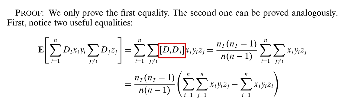
[Readings fixed by the printed text and used in every target] (a) $\mathbf{E}$ (also printed $E$), $\mathrm{Var}$ and all probability statements refer to the randomization distribution: $[T]$ is uniformly distributed over the $\binom{n}{n_T}$ subsets of $\{1,\ldots,n\}$ of size $n_T$, $[C]$ is its complement, both arms are non-empty ($1 \le n_T \le n-1$), and everything else is fixed. (b) Vectors are column vectors and a prime is a transpose; for $n$-vectors $a$, $b$ of scalars, $\overline{ab}$ is the average of the products $a_ib_i$, so $\overline{hy(1)}_T - \bar h_T\overline{y(1)}_T = \widehat{\mathrm{Cov}}_T(h, y(1))$, and $\overline{hy(1)} - \bar h\times\overline{y(1)}$ is the finite-population covariance of $h$ and $y(1)$ with divisor $n$. (c) $I_d^{-1}$ is printed for $I_d$ throughout, and the paper prints both $\hat N$ and $\widehat N$ (also $\hat N_T$, $\widehat N_T$) for the same objects. (d) In Assumption 1, $K$ is one constant, the same for every $n$: this is the reading the proofs use (the printed order of quantifiers is the clarity note P005-N002, not an error). (e) Assumption 2 is printed “for all $n$ large enough”; an exact finite-sample statement is read at a fixed $n$ at which (1) and (2) hold. Under Assumption 2, $\bar h = \frac1n\sum_i\|x_i\|_2^2 = \mathrm{tr}(\overline{xx'}) = d$, $h_i \le n$, and $\frac dn \le \kappa \le 1$ (the paper uses “$\kappa \in [\frac dn, 1]$” on p. 1516). (f) In Section 4, $\widehat\beta_{I,T}$ and $\widehat\beta_{I,C}$ are the within-arm slope vectors $\widehat L_T^{-1}\widehat N_T$ and $\widehat L_C^{-1}\widehat N_C$ defined there; their description as the coefficients on $D_ix_i$ and $x_i$ does not match parameterization (2), under which the coefficient on $D_ix_i$ is the difference of the two arm slopes (clarity note P005-E004, not an error). Every target uses the Section 4 definitions. (g) “Design matrices … are invertible” (footnote 4) is read as: $\widehat L$ (Section 3), respectively $\widehat L_T$ and $\widehat L_C$ (Section 4), is invertible under every assignment. (h) $O_p$, $o_p$, $O$, $o$ refer to a sequence of finite populations indexed by $n$, in which $d = d_n$, $n_T = n_{T,n}$, the covariates and the potential outcomes may all change with $n$; $\log$ is the natural logarithm.
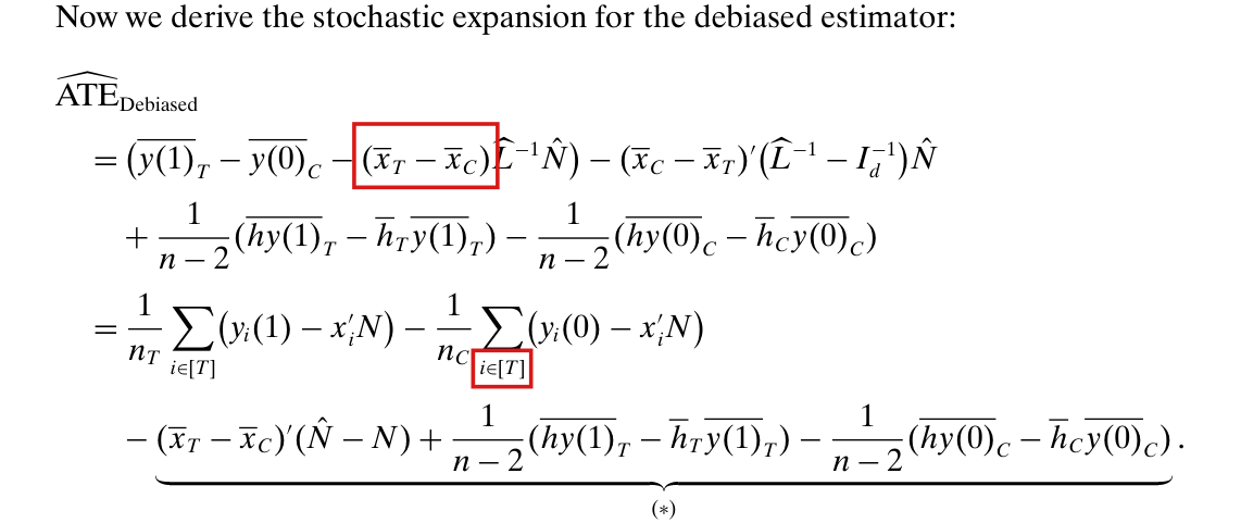
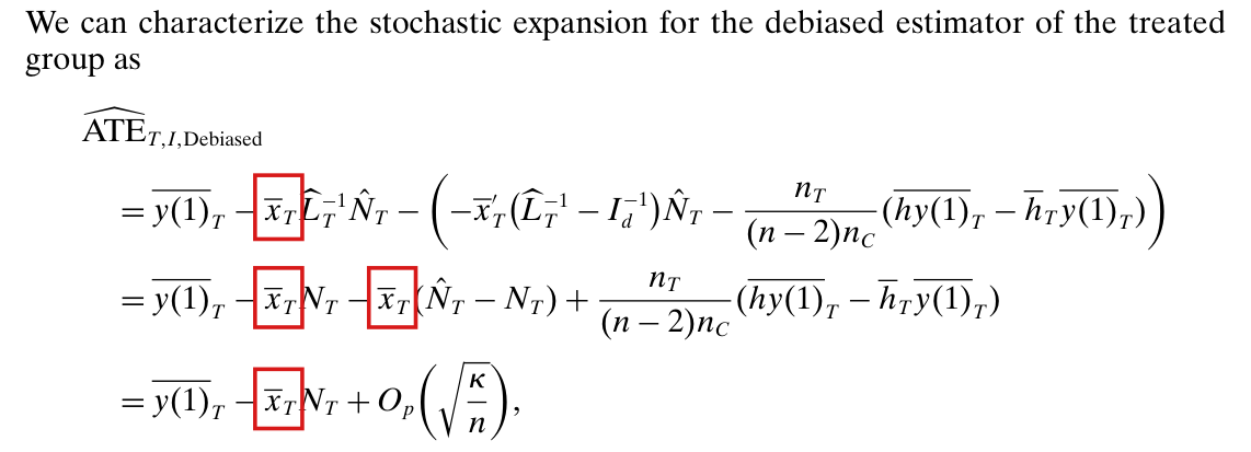
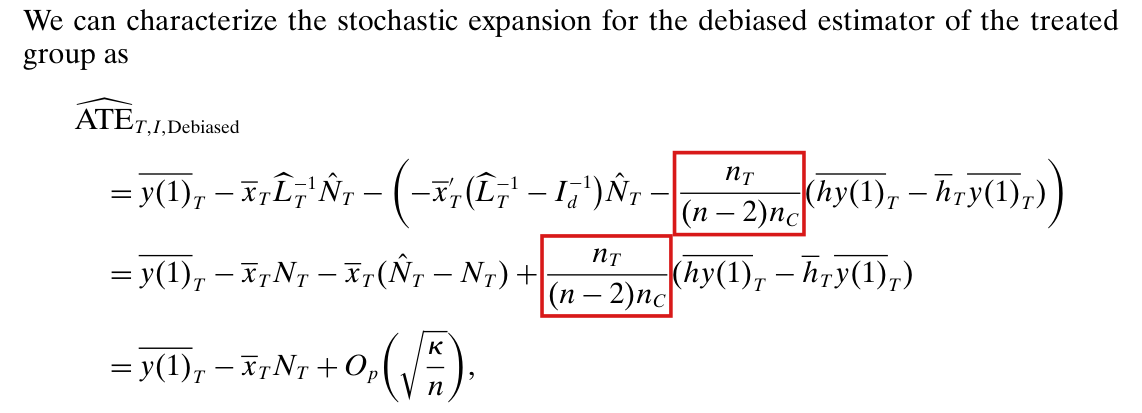
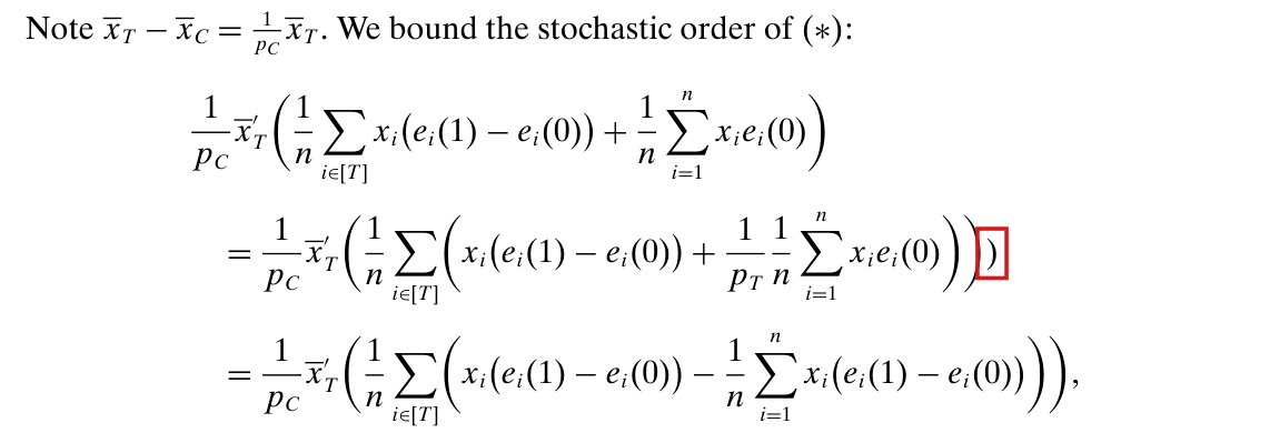
Effective claim (source TeX): [Printed, p. 1518 (PDF p. 17), last display of Appendix B.4] “We can characterize the stochastic expansion for the debiased estimator of the treated group as $$\widehat{\mathrm{ATE}}_{T,I,\mathrm{Debiased}} = \overline{y(1)}_T - \bar x_T\widehat L_T^{-1}\hat N_T - \Big(-\bar x_T'\big(\widehat L_T^{-1}-I_d^{-1}\big)\hat N_T - \frac{n_T}{(n-2)n_C}\big(\overline{hy(1)}_T-\bar h_T\overline{y(1)}_T\big)\Big)$$ $$= \overline{y(1)}_T - \bar x_TN_T - \bar x_T(\hat N_T-N_T) + \frac{n_T}{(n-2)n_C}\big(\overline{hy(1)}_T-\bar h_T\overline{y(1)}_T\big)$$ $$= \overline{y(1)}_T - \bar x_TN_T + O_p\Big(\sqrt{\frac{\kappa}{n}}\Big),$$” [continued on p. 1519 (PDF p. 18)] “using the stochastic order estimates we derived in the proof of Theorem 4.1 and the fact that $\kappa \in [\frac dn, 1]$.”
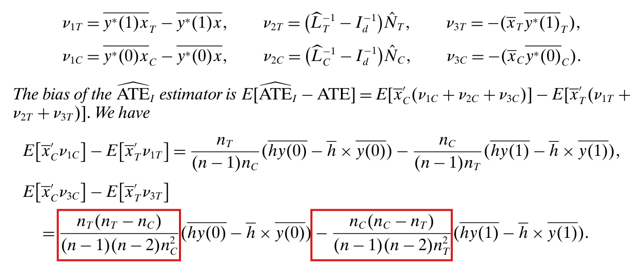
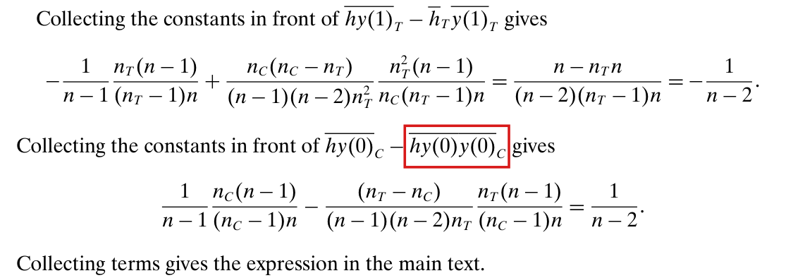
[Printed, same page, two displays earlier] “Collecting the constants in front of $(\overline{hy(1)}_T-\bar h_T\overline{y(1)}_T)$ gives $$\frac{n_C}{n(n_T-1)} - \frac{(n-n_T)(n-2n_T)}{(n-1)(n-2)n_T^2}\times\frac{n_T(n-1)}{(n_T-1)n} = \frac{n_C}{(n-2)n_T}.$$ Thus, an unbiased estimator for $\mathbf{E}[-\bar x_T'(\nu_{1T}+\nu_{2T}+\nu_{3T})]$ is $$-\frac{n_C}{(n-2)n_T}\big(\overline{hy(1)}_T-\bar h_T\overline{y(1)}_T\big) - \bar x_T'\big(\widehat L_T^{-1}-I_d^{-1}\big)\hat N_T.$$”
[What the printed display asserts] The “debiased estimator of the treated group” is $\overline{y(1)}_T - \bar x_T'\widehat\beta_{I,T}$ minus the estimator of its bias derived two displays earlier, and it is to be unbiased for $\overline{y(1)}$ (Theorem 4.2). After the inverse cancels, the printed first and second lines equal $P := \overline{y(1)}_T - \bar x_T'\hat N_T + \frac{n_T}{(n-2)n_C}\big(\overline{hy(1)}_T - \bar h_T\overline{y(1)}_T\big)$ (reading the unprimed $\bar x_T$ as $\bar x_T'$: the missing transposes of P005-E010, restored in P005-T11), whereas the estimator derived two displays earlier gives $Q := \overline{y(1)}_T - \bar x_T'\hat N_T + \frac{n_C}{(n-2)n_T}\big(\overline{hy(1)}_T - \bar h_T\overline{y(1)}_T\big)$.
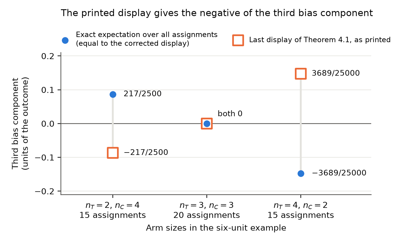
[Counterexample] Take $n = 6$, $n_T = 2$, $n_C = 4$, $d = 1$, $a = (-3, -2, -1, 0, 1, 5)$ and $x_i = \sqrt{3/20}\,a_i$, $y_i(1) = a_i^2$, that is, $y(1) = (9, 4, 1, 0, 1, 25)$, and $y(0) = (0, \ldots, 0)$. Then:
(i) [The paper's conditions hold at this $n$] $\bar x = 0$ and $\overline{x^2} = \frac{3}{20}\cdot\frac{40}{6} = 1$ (Assumption 2); the six covariate values are distinct, so $\widehat L_T = \frac{3}{20}(\overline{a^2}_T - \bar a_T^2) > 0$ and $\widehat L_C = \frac{3}{20}(\overline{a^2}_C - \bar a_C^2) > 0$ under each of the 15 assignments (footnote 4); $h_i = x_i^2 = \frac{3}{20}a_i^2$ and $\bar h = 1$; $\overline{y(1)} = \frac{20}{3}$; $S_1 := \overline{hy(1)} - \bar h\times\overline{y(1)} = \frac{343}{30}$.
(ii) With the printed weight $\frac{n_T}{(n-2)n_C} = \frac18$: $\mathbf{E}[P] = \frac{4913}{1200} \ne \frac{20}{3} = \overline{y(1)}$.
(iii) With the derived weight $\frac{n_C}{(n-2)n_T} = \frac12$: $\mathbf{E}[Q] = \frac{20}{3} = \overline{y(1)}$.
(iv) $P - Q = \big(\frac{n_T}{(n-2)n_C} - \frac{n_C}{(n-2)n_T}\big)\widehat{\mathrm{Cov}}_T(h, y(1)) = -\frac38\widehat{\mathrm{Cov}}_T(h, y(1))$, and $\mathbf{E}[P] - \mathbf{E}[Q] = -\frac38\cdot\frac{(n_T-1)n}{n_T(n-1)}S_1 = -\frac38\cdot\frac35\cdot\frac{343}{30} = -\frac{1029}{400}$.
(In rational terms: $\bar x_T'\hat N_T = \frac{3}{20}\,\bar a_T\big(\overline{ay(1)}_T - \bar a_T\overline{y(1)}_T\big)$ and $\widehat{\mathrm{Cov}}_T(h, y(1)) = \frac{3}{20}\big(\overline{a^2y(1)}_T - \overline{a^2}_T\overline{y(1)}_T\big)$.) So the printed display is not the treated-group part of the debiased estimator of Theorem 4.2, and the expression it prints is not unbiased for $\overline{y(1)}$ in an unbalanced design; it contradicts the unbiased estimator printed two displays above it.
: SAP.P005a.T10WholeStatement
Theorem: SAP.P005a.T10
Statement hash: ddfdaacefaec314fa62f4b65343aaf0e30200fa7e230e62455df4d3670390a6e
Statement definition: SAP.P005a.T10WholeStatement
Certificate. 20261104T172639Z
Declaration review: faithful; 2026-11-04T18:12:01Z; binding v2
Evidence scope: Certification checks formal proof objects. Statement fidelity is a model judgment. Author review is separate.
Proof dependencies: Independently extracted
Manifest annotation reconciliation: Effective use follows the source-bound dependency observation; original annotations are retained in the crosswalk.
AronowAudit.P005.sampleCov_scale_both: observed used
AronowAudit.P005.sampleCov_scale_left: observed used
AronowAudit.P005.scalar_armL_det: observed used
AronowAudit.P005.scalar_dot_armN: observed used
AronowAudit.P005.scalar_leverage: observed used
AronowAudit.P005.standardized_scalar: observed used
Source and evidence metadata · sap-2026-11-08-assured-release