P010-E013 Moderate
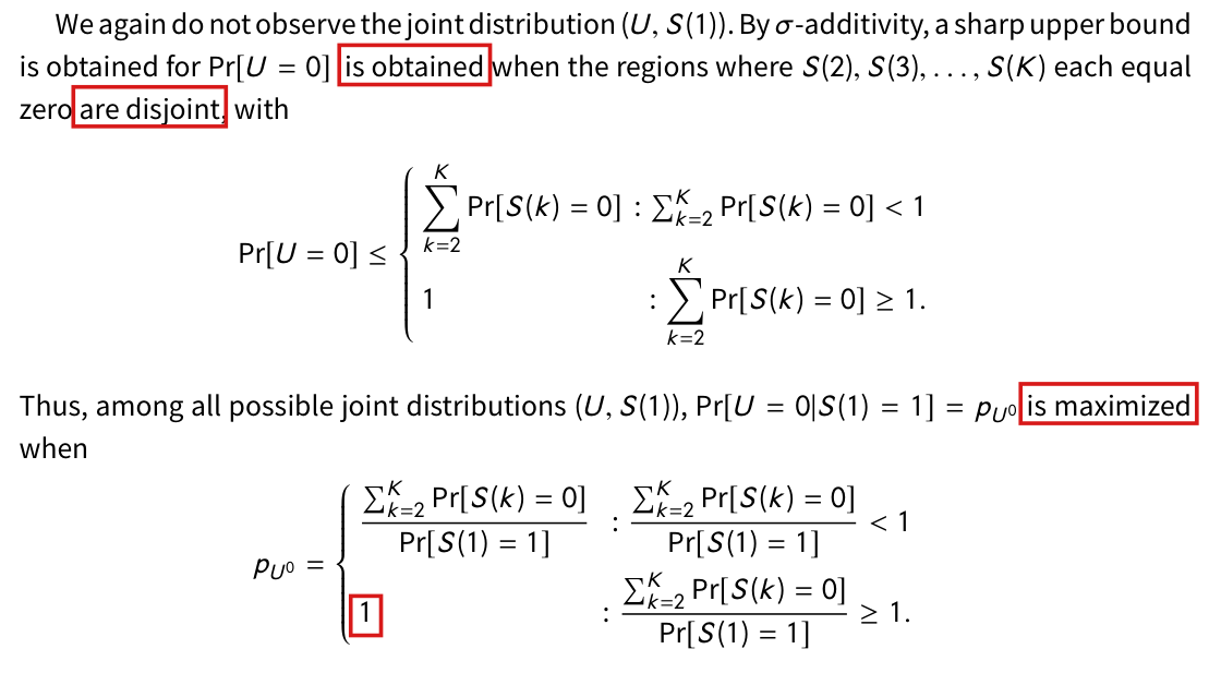
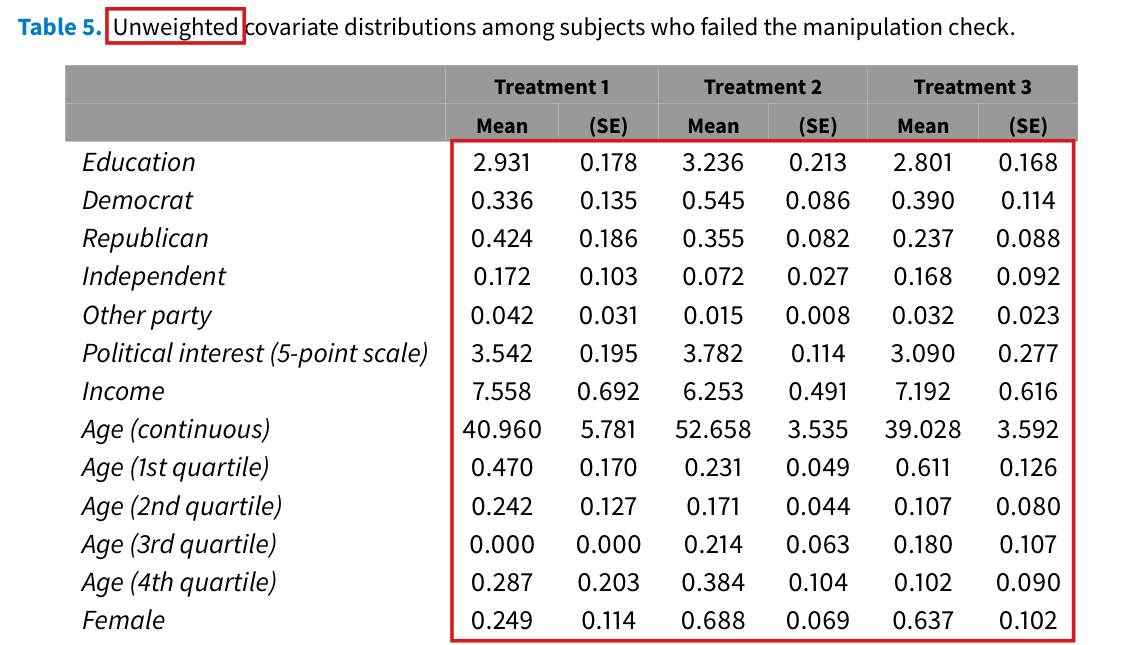
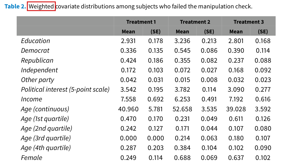
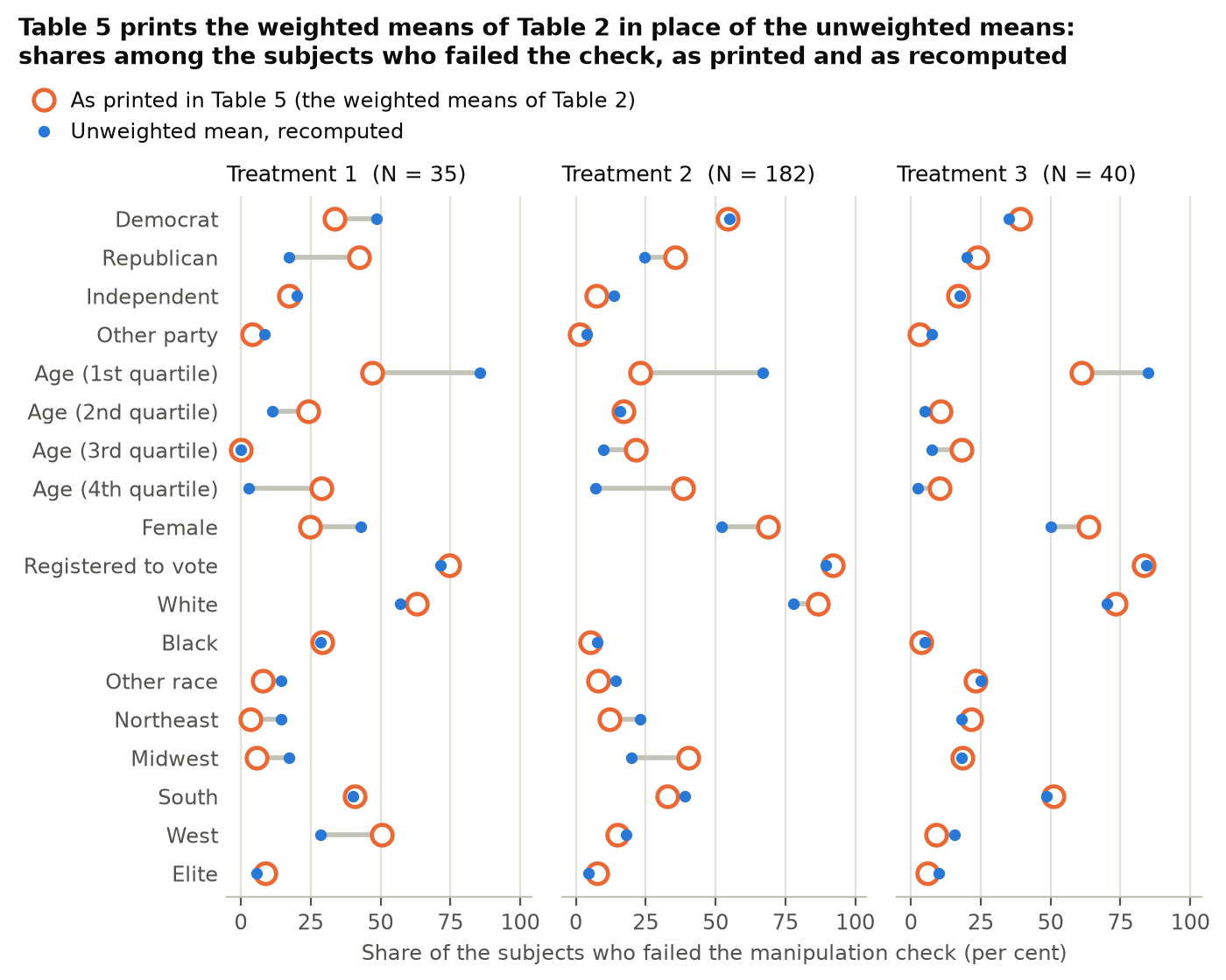
Table 5 is captioned as the unweighted covariate distributions of the subjects who failed the manipulation check, but its entries are the weighted ones of Table 2; 74 of its 75 means differ from the unweighted means.
Appendix E, Table 5, all entries, p. 586 (PDF p. 15); compare Table 2, p. 582 (PDF p. 11); replication files, abp_replication.R, line 1261
As printed
Table 5, p. 586. Table 5. Unweighted covariate distributions among subjects who failed the manipulation check.
| Treatment 1 | Treatment 2 | Treatment 3 | ||||
|---|---|---|---|---|---|---|
| Mean | (SE) | Mean | (SE) | Mean | (SE) | |
| Education | 2.931 | 0.178 | 3.236 | 0.213 | 2.801 | 0.168 |
| Democrat | 0.336 | 0.135 | 0.545 | 0.086 | 0.390 | 0.114 |
| Republican | 0.424 | 0.186 | 0.355 | 0.082 | 0.237 | 0.088 |
| Independent | 0.172 | 0.103 | 0.072 | 0.027 | 0.168 | 0.092 |
| Other party | 0.042 | 0.031 | 0.015 | 0.008 | 0.032 | 0.023 |
| Political interest (5-point scale) | 3.542 | 0.195 | 3.782 | 0.114 | 3.090 | 0.277 |
| Income | 7.558 | 0.692 | 6.253 | 0.491 | 7.192 | 0.616 |
| Age (continuous) | 40.960 | 5.781 | 52.658 | 3.535 | 39.028 | 3.592 |
| Age (1st quartile) | 0.470 | 0.170 | 0.231 | 0.049 | 0.611 | 0.126 |
| Age (2nd quartile) | 0.242 | 0.127 | 0.171 | 0.044 | 0.107 | 0.080 |
| Age (3rd quartile) | 0.000 | 0.000 | 0.214 | 0.063 | 0.180 | 0.107 |
| Age (4th quartile) | 0.287 | 0.203 | 0.384 | 0.104 | 0.102 | 0.090 |
| Female | 0.249 | 0.114 | 0.688 | 0.069 | 0.637 | 0.102 |
| Ideology (5-point scale) | 3.116 | 0.318 | 3.019 | 0.145 | 2.874 | 0.202 |
| News interest (4-point scale) | 1.959 | 0.290 | 1.636 | 0.113 | 2.458 | 0.265 |
| Registered to vote | 0.746 | 0.119 | 0.919 | 0.041 | 0.832 | 0.092 |
| White | 0.630 | 0.141 | 0.867 | 0.035 | 0.733 | 0.095 |
| Black | 0.292 | 0.125 | 0.053 | 0.020 | 0.036 | 0.027 |
| Other race | 0.078 | 0.048 | 0.080 | 0.025 | 0.231 | 0.093 |
| Religious importance | 4.680 | 0.457 | 4.623 | 0.257 | 3.774 | 0.391 |
| Northeast | 0.034 | 0.023 | 0.121 | 0.037 | 0.217 | 0.104 |
| Midwest | 0.056 | 0.035 | 0.404 | 0.099 | 0.183 | 0.093 |
| South | 0.406 | 0.149 | 0.326 | 0.074 | 0.511 | 0.111 |
| West | 0.504 | 0.166 | 0.149 | 0.041 | 0.089 | 0.042 |
| Elite | 0.089 | 0.073 | 0.076 | 0.046 | 0.059 | 0.037 |
| Observations |
Replication files, abp_replication.R, line 1261 (not printed in the article).
The problem
Appendix E announces the unweighted covariate profiles of the subjects, by treatment and by performance on the manipulation check, as the counterpart of the weighted profiles of Appendix D. Table 5 does not contain them. Its 150 numerical entries and its three numbers of observations are those of Table 2, which gives the weighted profiles of the subjects who failed. The cause is one line of the replication code. The script computes the unweighted table failed.tab in lines 1246–1258, and in line 1261, where it formats the table, it overwrites it with the formatted weighted table w.failed.tab. The two files tab_2.txt and tab_5.txt saved with the replication files are identical byte for byte.
The unweighted profiles of the subjects who failed are not printed anywhere in the paper, and they differ from the printed values in 74 of the 75 means. The share of women among these subjects is 42.9, 52.2 and 50.0 percent in the three treatments, where Table 5 prints 24.9, 68.8 and 63.7 percent. Their mean age is 28.6, 35.9 and 30.8 years, where Table 5 prints 41.0, 52.7 and 39.0. Table 5 therefore gives the wrong unweighted composition of the subjects who would be dropped.
Evidence an exact counterexample
The evidence is a recalculation from the public data in exact arithmetic, with two checks of the printed tables against one another. Applying to the public data the recoding of the replication script, with its replacement of missing covariates by the mean over the replication sample, I obtain the 63 means of the 21 covariates that need no confidential input. Among the subjects who failed, of , of and of are women. The printed shares cannot be unweighted shares. A count with , or equal to 0.249, 0.688 or 0.637 after rounding would have to lie in , or , and none of these intervals contains an integer.
The twelve means of the age quartiles depend on quartiles of the sample of Press, Sagan and Valentino, which is not public. They can be recovered from Tables 6 and 7. Since every sample there has fewer than 1,000 subjects, each share printed to three decimals fixes one integer count. The count among the subjects who failed is the count among all subjects minus the count among those who passed. The counts are , and for the three treatments. Classifying the ages in the public data at the boundaries 39, 50 and 59 reproduces every one of these counts.
For any covariate, , where the subscripts denote all subjects, those who passed and those who failed. With the printed means of age in Treatment 2, the right side divided by is , where Table 7 prints . The gap is , and rounding allows at most . With the recomputed means, all 75 identities hold exactly, and all 150 means of Tables 6 and 7 are reproduced to the printed precision. The one mean of Table 5 that is unchanged is the zero for the third age quartile in Treatment 1.
The standard errors of the paper are bootstrap estimates from 10,000 samples. The standard deviation of the mean of a bootstrap sample has the closed form . For the share of women in Treatment 1 it is , where Table 5 prints .
What survives
Table 2 and the comparison in Section 3 that cites it, with 63.7 and 24.9 percent of women among the subjects who failed under Treatments 3 and 1, are explicitly weighted and are not affected by this error. I could not recompute the weighted values, since the weights require data that are not public. Tables 6 and 7 are produced from other objects of the code, and their means are reproduced. No figure, estimate, bound or theoretical result of the paper uses Table 5.
Corrected
Replication files, line 1261.
Table 5. Unweighted covariate distributions among subjects who failed the manipulation check.
| Covariate | Treatment 1 | Treatment 2 | Treatment 3 |
|---|---|---|---|
| Education | 3.457 (0.199) | 4.033 (0.095) | 3.275 (0.190) |
| Democrat | 0.486 (0.084) | 0.549 (0.037) | 0.350 (0.075) |
| Republican | 0.171 (0.064) | 0.247 (0.032) | 0.200 (0.063) |
| Independent | 0.200 (0.068) | 0.137 (0.026) | 0.175 (0.060) |
| Other party | 0.086 (0.047) | 0.038 (0.014) | 0.075 (0.042) |
| Political interest (5-point scale) | 3.200 (0.139) | 3.313 (0.071) | 3.108 (0.173) |
| Income | 7.236 (0.594) | 6.435 (0.252) | 6.808 (0.482) |
| Age (continuous) | 28.571 (1.577) | 35.890 (0.927) | 30.750 (1.703) |
| Age (1st quartile) | 0.857 (0.059) | 0.670 (0.035) | 0.850 (0.056) |
| Age (2nd quartile) | 0.114 (0.054) | 0.159 (0.027) | 0.050 (0.034) |
| Age (3rd quartile) | 0.000 (0.000) | 0.099 (0.022) | 0.075 (0.042) |
| Age (4th quartile) | 0.029 (0.028) | 0.071 (0.019) | 0.025 (0.025) |
| Female | 0.429 (0.084) | 0.522 (0.037) | 0.500 (0.079) |
| Ideology (5-point scale) | 2.646 (0.161) | 2.674 (0.076) | 2.780 (0.167) |
| News interest (4-point scale) | 2.400 (0.135) | 2.100 (0.070) | 2.334 (0.138) |
| Registered to vote | 0.714 (0.076) | 0.894 (0.023) | 0.843 (0.056) |
| White | 0.571 (0.084) | 0.780 (0.031) | 0.700 (0.072) |
| Black | 0.286 (0.076) | 0.077 (0.020) | 0.050 (0.034) |
| Other race | 0.143 (0.059) | 0.143 (0.026) | 0.250 (0.068) |
| Religious importance | 3.171 (0.327) | 3.214 (0.147) | 3.075 (0.286) |
| Northeast | 0.143 (0.059) | 0.231 (0.031) | 0.180 (0.060) |
| Midwest | 0.171 (0.064) | 0.198 (0.030) | 0.181 (0.060) |
| South | 0.400 (0.083) | 0.390 (0.036) | 0.484 (0.078) |
| West | 0.286 (0.076) | 0.181 (0.029) | 0.156 (0.056) |
| Elite | 0.057 (0.039) | 0.044 (0.015) | 0.100 (0.047) |
| Observations |
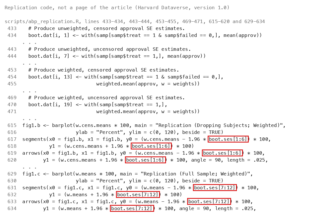
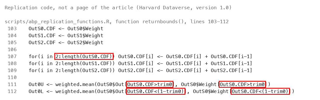
![Listing of R code with line numbers. Lines 433 to 434 carry the comment Produce unweighted, censored approval SE estimates and assign boot.dat column 1. Lines 443 to 444 do the same for unweighted, uncensored estimates and column 7. Lines 453 to 455 carry the comment Produce weighted, censored approval SE estimates and assign column 13 with weighted.mean. Lines 469 to 471 do the same for weighted, uncensored estimates and column 19. Lines 615 to 620 draw Panel B, titled Replication (Dropping Subjects; Weighted), with interval bars at w.cens.means plus or minus 1.96 times boot.ses[1:6]. Lines 629 to 634 draw Panel C, titled Replication (Full Sample; Weighted), with interval bars at w.means plus or minus 1.96 times boot.ses[7:12]. Red outlines surround the four occurrences of boot.ses[1:6] and the four occurrences of boot.ses[7:12].](exhibits/P010-E014-code.png)

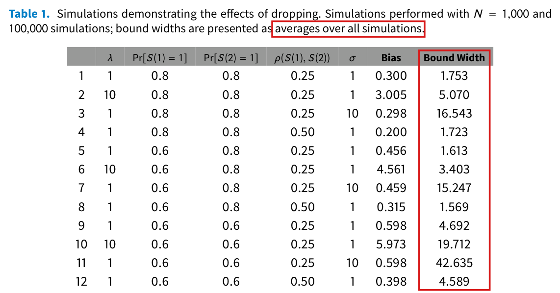
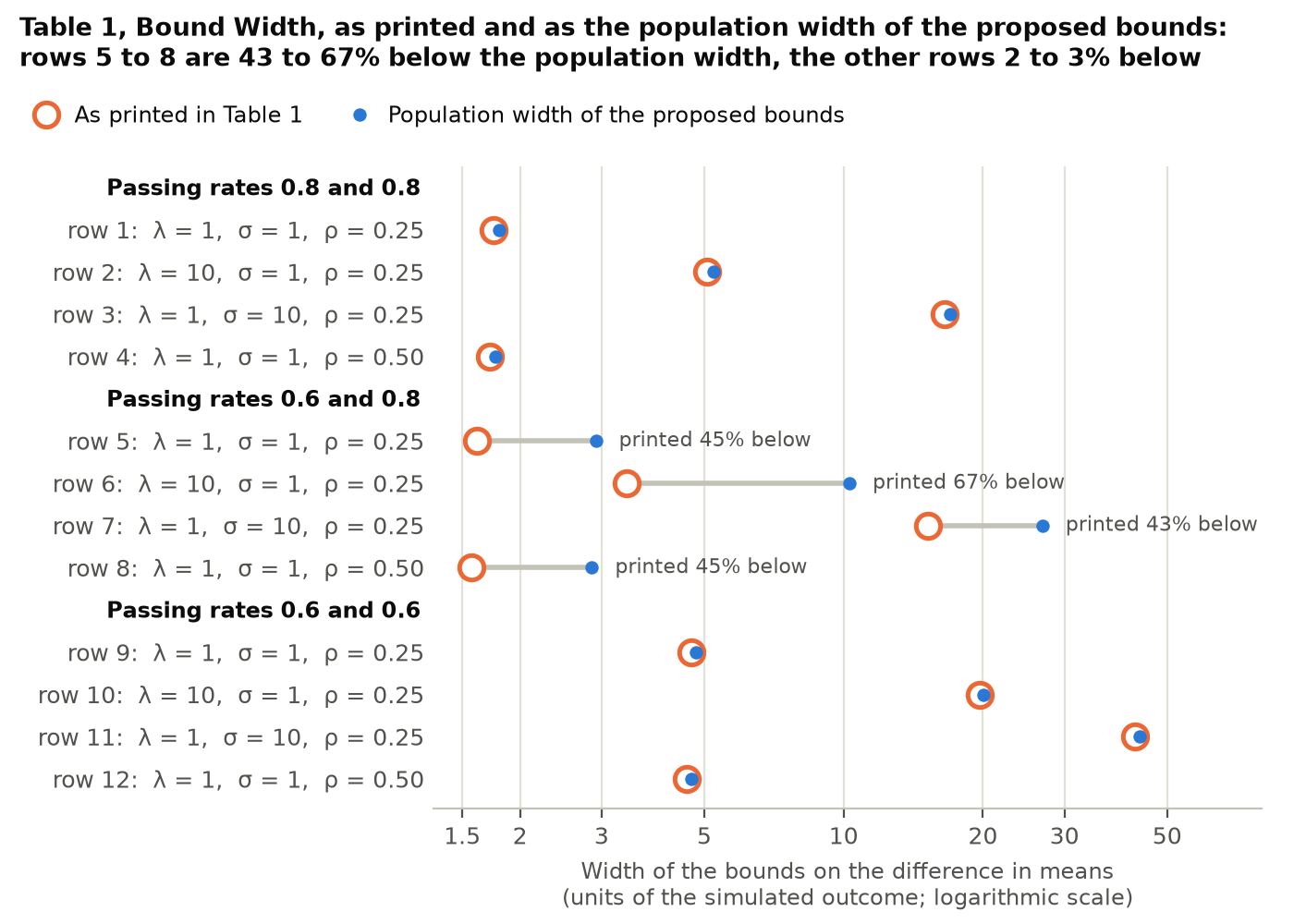
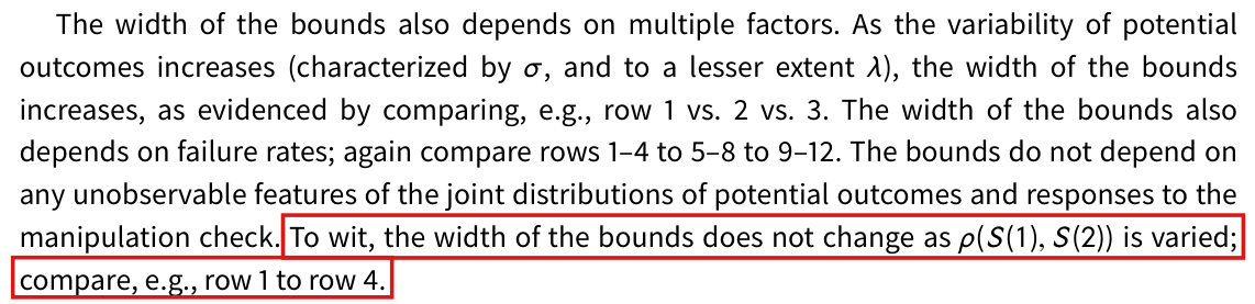
![Crop of Table 1 with its caption. The caption reads: Table 1. Simulations demonstrating the effects of dropping. Simulations performed with N = 1,000 and 100,000 simulations; bound widths are presented as averages over all simulations. The table has twelve numbered rows and the columns lambda, Pr[S(1) = 1], Pr[S(2) = 1], rho(S(1), S(2)), sigma, Bias and Bound Width. The Bound Width entries in rows 1 to 12 are 1.753, 5.070, 16.543, 1.723, 1.613, 3.403, 15.247, 1.569, 4.692, 19.712, 42.635 and 4.589. Rows 1 to 4 have passing rates 0.8 and 0.8, rows 5 to 8 have 0.6 and 0.8, and rows 9 to 12 have 0.6 and 0.6. Red outlines surround the words averages over all simulations in the caption and the whole Bound Width column with its heading.](exhibits/P010-E016.png)


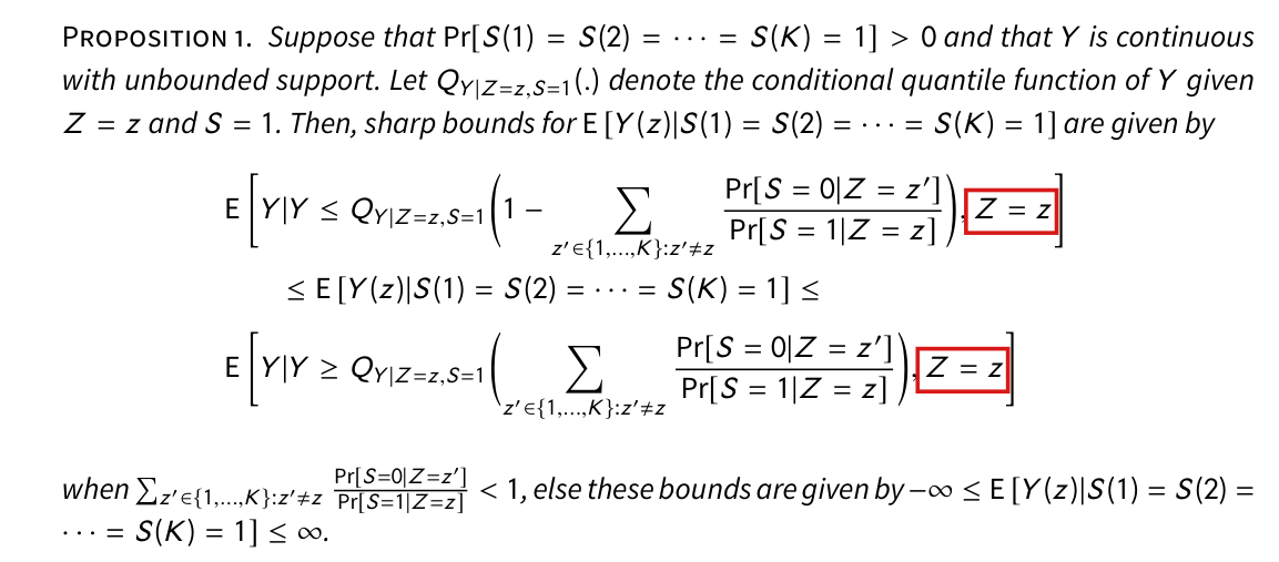
![Crop of Proposition 1. After the hypotheses, the display gives a lower bound E[Y | Y less than or equal to the quantile of Y given Z = z, S = 1 evaluated at one minus the sum over the other arms of Pr[S = 0 | Z = z'] divided by Pr[S = 1 | Z = z], Z = z], then the target E[Y(z) | S(1) = S(2) = ... = S(K) = 1], then an upper bound of the same form with Y greater than or equal to the quantile evaluated at the sum. Red outlines surround the two occurrences of Z = z at the end of the outer expectations. The last two lines say that these bounds hold when the sum is below 1, else the bounds are minus infinity and infinity.](exhibits/P010-E001.png)
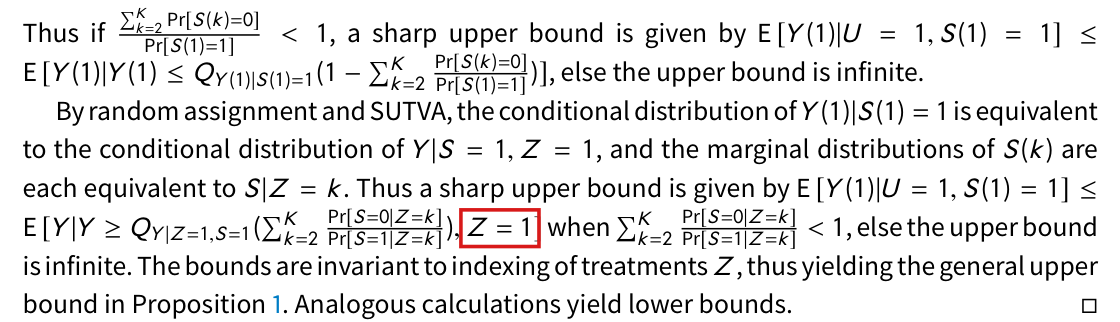
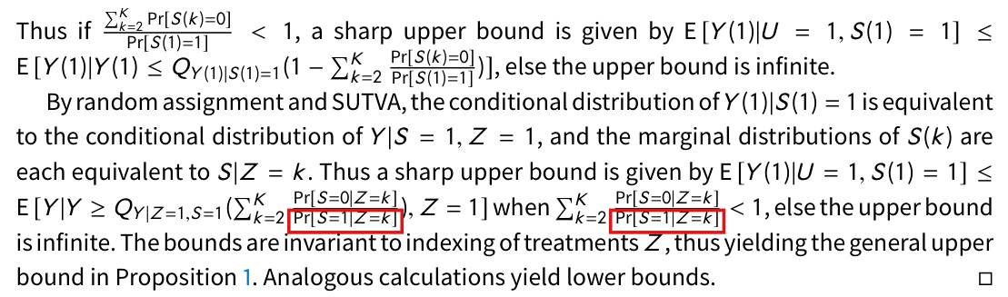
![Crop of the last eight lines of the proof of Proposition 1. The final bound reads: E[Y(1) | U = 1, S(1) = 1] is at most E[Y | Y greater than or equal to the quantile of Y given Z = 1, S = 1 evaluated at the sum over k from 2 to K of Pr[S = 0 | Z = k] over Pr[S = 1 | Z = k], Z = 1] when that sum is below 1, else the upper bound is infinite. A red outline surrounds Z = 1 at the end of the expectation.](exhibits/P010-E001-b.png)
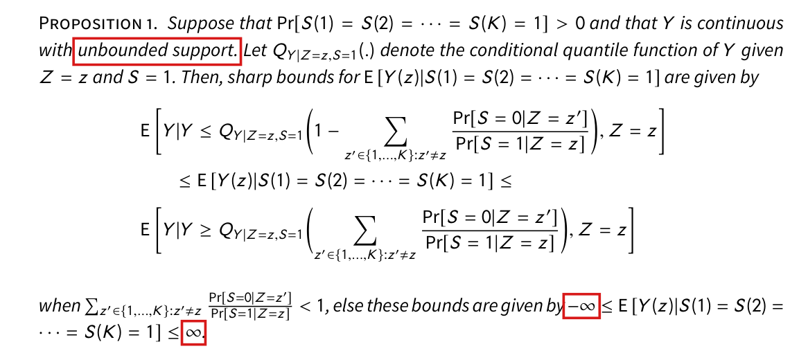
![Crop of Proposition 1. The first sentence reads: Suppose that Pr[S(1) = S(2) = ... = S(K) = 1] > 0 and that Y is continuous with unbounded support. After the displayed trimming bounds, the last two lines read: when the sum of Pr[S = 0 | Z = z'] over Pr[S = 1 | Z = z] is less than 1, else these bounds are given by minus infinity less than or equal to E[Y(z) | S(1) = S(2) = ... = S(K) = 1] less than or equal to infinity. Red outlines surround the words unbounded support, the symbol for minus infinity and the symbol for infinity.](exhibits/P010-E002.png)


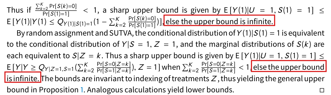
![Crop of the last seven lines of the proof of Proposition 1. The first two lines read: Thus if the sum over k from 2 to K of Pr[S(k) = 0] divided by Pr[S(1) = 1] is less than 1, a sharp upper bound is given by E[Y(1) given U = 1, S(1) = 1] at most E[Y(1) given Y(1) at most Q of 1 minus the sum of Pr[S(k) = 0] over Pr[S(1) = 1]], else the upper bound is infinite. The next lines read: By random assignment and SUTVA, the conditional distribution of Y(1) given S(1) = 1 is equivalent to the conditional distribution of Y given S = 1, Z = 1, and the marginal distributions of S(k) are each equivalent to S given Z = k. Thus a sharp upper bound is given by E[Y(1) given U = 1, S(1) = 1] at most E[Y given Y at least Q of the sum over k from 2 to K of Pr[S = 0 given Z = k] over Pr[S = 1 given Z = k], Z = 1] when the sum over k from 2 to K of Pr[S = 0 given Z = k] over Pr[S = 1 given Z = k] is less than 1, else the upper bound is infinite. The bounds are invariant to indexing of treatments Z, thus yielding the general upper bound in Proposition 1. Analogous calculations yield lower bounds. Red outlines surround the two denominators Pr[S = 1 given Z = k].](exhibits/P010-E005.png)


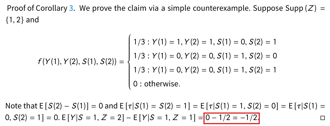
![Crop of the proof of Corollary 3. It reads: Proof of Corollary 3. We prove the claim via a simple counterexample. Suppose Supp(Z) = {1, 2} and f(Y(1), Y(2), S(1), S(2)) equals 1/3 for Y(1) = 1, Y(2) = 1, S(1) = 0, S(2) = 1; 1/3 for Y(1) = 0, Y(2) = 0, S(1) = 1, S(2) = 0; 1/3 for Y(1) = 0, Y(2) = 0, S(1) = 1, S(2) = 1; and 0 otherwise. Note that E[S(2) minus S(1)] = 0 and E[tau given S(1) = S(2) = 1] = E[tau given S(1) = 1, S(2) = 0] = E[tau given S(1) = 0, S(2) = 1] = 0. E[Y given S = 1, Z = 2] minus E[Y given S = 1, Z = 1] = 0 minus 1/2 = minus 1/2. A red outline surrounds the final arithmetic, 0 minus 1/2 = minus 1/2.](exhibits/P010-E010.png)


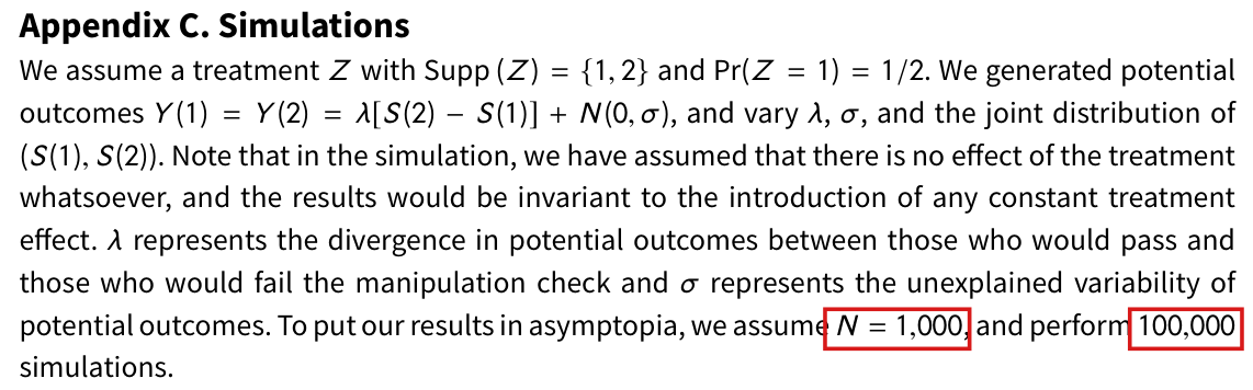
![Crop of the heading Appendix C. Simulations and its first paragraph. It reads: We assume a treatment Z with Supp(Z) = {1, 2} and Pr(Z = 1) = 1/2. We generated potential outcomes Y(1) = Y(2) = lambda [S(2) minus S(1)] + N(0, sigma), and vary lambda, sigma, and the joint distribution of (S(1), S(2)). Note that in the simulation, we have assumed that there is no effect of the treatment whatsoever, and the results would be invariant to the introduction of any constant treatment effect. Lambda represents the divergence in potential outcomes between those who would pass and those who would fail the manipulation check and sigma represents the unexplained variability of potential outcomes. To put our results in asymptopia, we assume N = 1,000, and perform 100,000 simulations. Red outlines surround N = 1,000 and 100,000 in the last sentence.](exhibits/P010-E015.png)
![Crop of the caption of Table 1 and the first two rows of the table. The caption reads: Table 1. Simulations demonstrating the effects of dropping. Simulations performed with N = 1,000 and 100,000 simulations; bound widths are presented as averages over all simulations. The column heads are lambda, Pr[S(1) = 1], Pr[S(2) = 1], rho(S(1), S(2)), sigma, Bias and Bound Width, and the first two rows are 1, 1, 0.8, 0.8, 0.25, 1, 0.300, 1.753 and 2, 10, 0.8, 0.8, 0.25, 1, 3.005, 5.070. Red outlines surround N = 1,000 at the end of the first line of the caption and 100,000 at the start of the second.](exhibits/P010-E015-b.png)
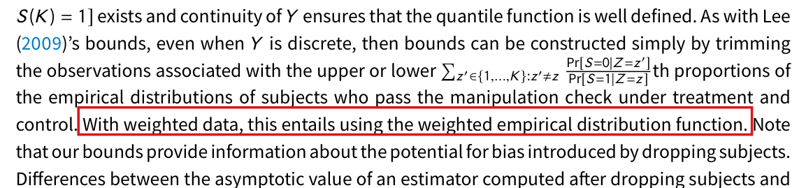
![Crop of seven lines of the paragraph that follows Proposition 1. It says that bounds can be constructed by trimming the observations associated with the upper or lower proportions, given by the sum of Pr[S = 0 | Z = z'] over Pr[S = 1 | Z = z], of the empirical distributions of subjects who pass the manipulation check. A red outline surrounds the sentence: With weighted data, this entails using the weighted empirical distribution function.](exhibits/P010-E017.png)


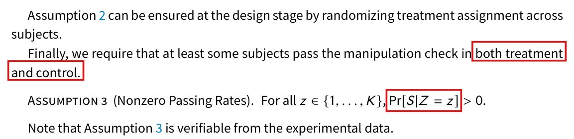
![Crop of six lines. The text reads: Finally, we require that at least some subjects pass the manipulation check in both treatment and control. Assumption 3 (Nonzero Passing Rates). For all z in the set 1 to K, Pr[S | Z = z] > 0. Note that Assumption 3 is verifiable from the experimental data. Red outlines surround the words both treatment and control, across a line break, and the expression Pr[S | Z = z], in which S is not followed by = 1.](exhibits/P010-N002.png)
![Crop of six lines. Corollary 1 reads: If Pr[S(1) = S(2) = ... = S(K)] = 1, then E[Y | S = 1, Z = z] - E[Y | S = 1, Z = z'] = E[Y(z) - Y(z')] | S(1) = S(2) = ... = S(K) = 1]. A red outline surrounds the closing square bracket that follows Y(z') and precedes the conditioning bar.](exhibits/P010-N003.png)
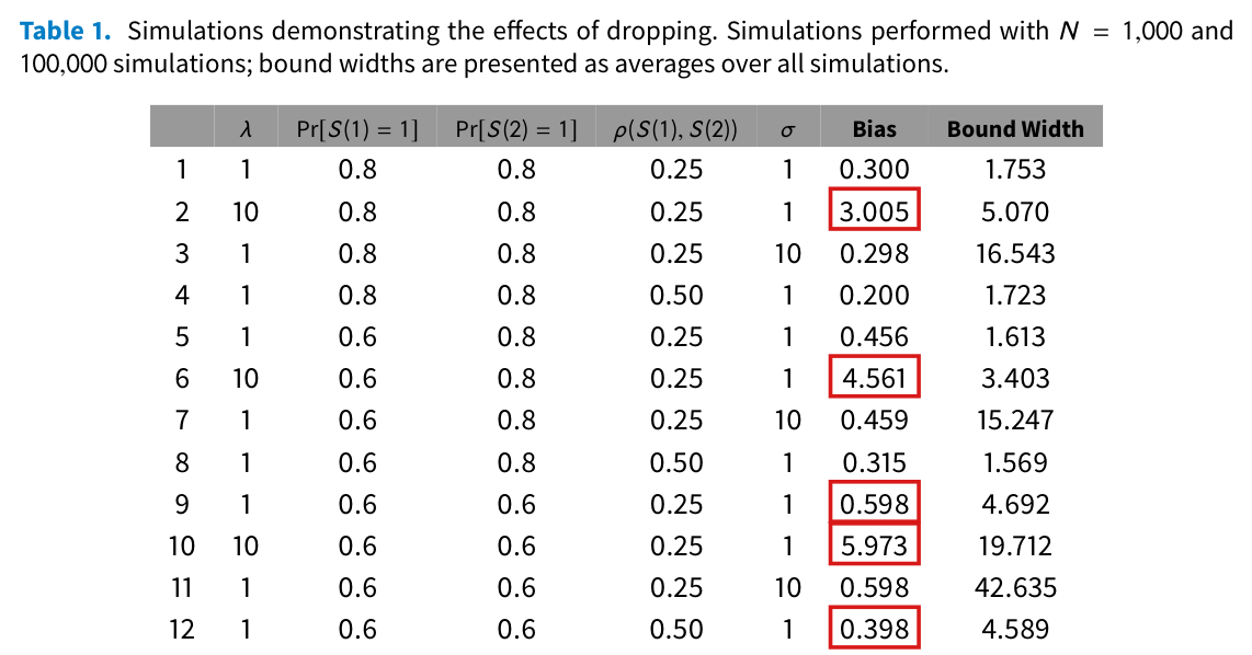
![Crop of Table 1 with its caption. The table has twelve numbered rows and the columns lambda, Pr[S(1) = 1], Pr[S(2) = 1], rho(S(1), S(2)), sigma, Bias and Bound Width. The Bias entries in rows 1 to 12 are 0.300, 3.005, 0.298, 0.200, 0.456, 4.561, 0.459, 0.315, 0.598, 5.973, 0.598 and 0.398. The column rho(S(1), S(2)) reads 0.25 in every row except rows 4, 8 and 12, where it reads 0.50. Red outlines surround the Bias entries 3.005 in row 2, 4.561 in row 6, 0.598 in row 9, 5.973 in row 10 and 0.398 in row 12.](exhibits/P010-N014.png)
![Crop of five lines. After the end of Proposition 1, the text reads: Assuming that Pr[S(1) = S(2) = ... = S(K) = 1] > 0 ensures that E[Y(z) | S(1) = S(2) = ... = S(K) = 1] exists and continuity of Y ensures that the quantile function is well defined. As with Lee (2009)'s bounds, even when Y is discrete, then bounds can be constructed simply by trimming. A red outline surrounds the words from Assuming that to exists, across a line break.](exhibits/P010-E003.png)
![Crop of a paragraph and two displays from the proof of Proposition 1. The text reads: We again do not observe the joint distribution (U, S(1)). By sigma-additivity, a sharp upper bound is obtained for Pr[U = 0] is obtained when the regions where S(2), S(3), ..., S(K) each equal zero are disjoint, with. The first display bounds Pr[U = 0] above by the sum over k from 2 to K of Pr[S(k) = 0] when that sum is less than 1, and by 1 when the sum is at least 1. The text continues: Thus, among all possible joint distributions (U, S(1)), Pr[U = 0 given S(1) = 1] = p U 0 is maximized when. The second display sets p U 0 equal to the sum of Pr[S(k) = 0] divided by Pr[S(1) = 1] when that ratio is less than 1, and equal to 1 when the ratio is at least 1. Red outlines surround the second occurrence of the words is obtained, the words are disjoint, the words is maximized, and the value 1 in the second case of the second display.](exhibits/P010-E006.png)

![Crop of five lines. The sentence reads: There is a condition under which dropping subjects who fail a manipulation check recovers this quantity, namely that in which the treatment assigned to a subject is statistically unrelated to whether or not that subject passes or fails the manipulation. Below it, Corollary 1 begins: If Pr[S(1) = S(2) = ... = S(K)] = 1. A red outline surrounds the words statistically unrelated to.](exhibits/P010-E008-b.png)


My comment and the history of this entry
Suggested classification: Minor error.
My position My comment above; I suggested a Minor error.
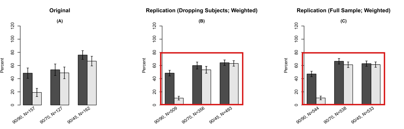
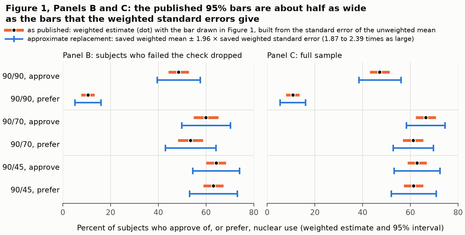
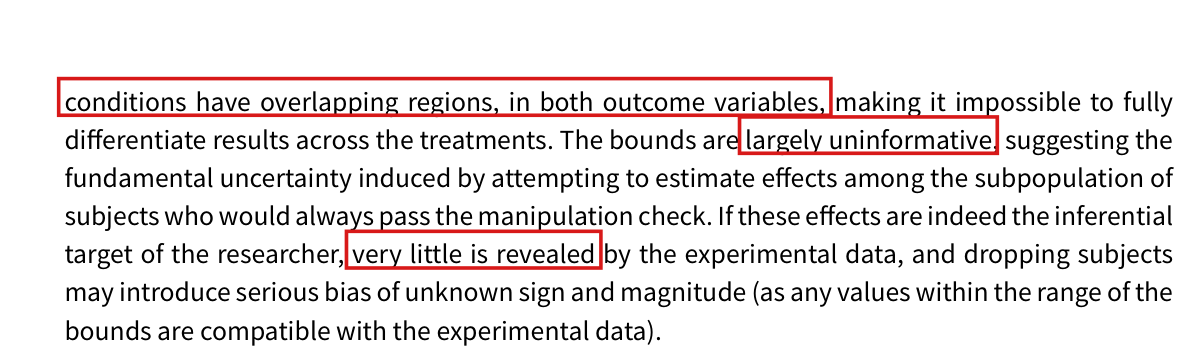
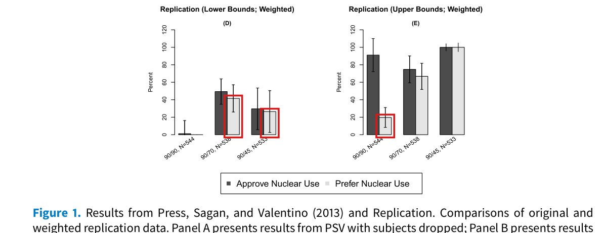
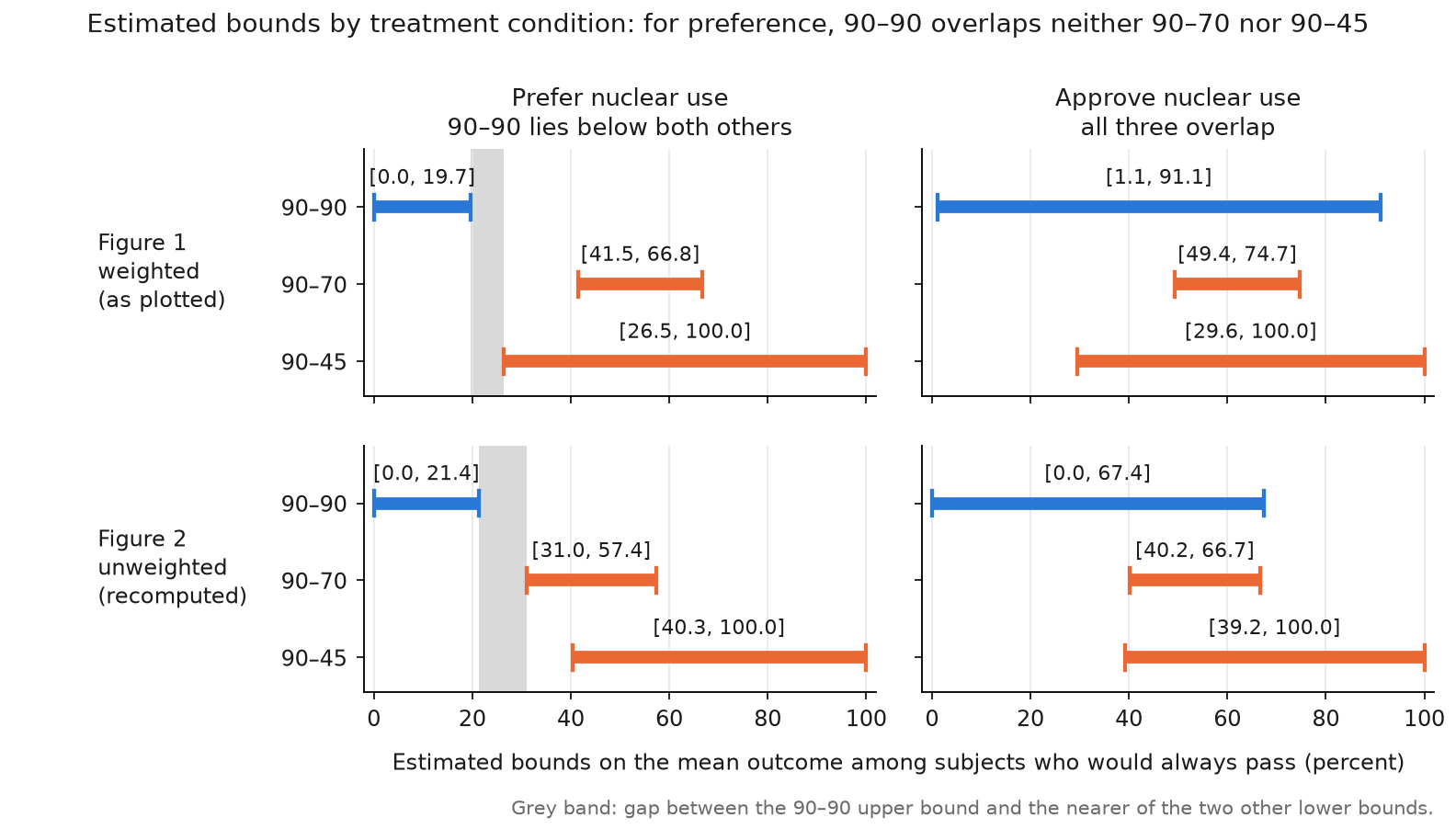
The models’ position The broad warning and the plotted values survive, but the claim in the text about the overlap of the intervals is false and hides two estimated preference contrasts. A reader who relies on the text takes away materially less than the estimates show: Moderate.