LLM-generated corrections to the published research of P. M. Aronow

Journal article P014

Corrections to: The Regression Discontinuity Design under Interference: A Local Randomization-Based Approach

P. M. Aronow, Nicole E. Basta, and M. Elizabeth Halloran (2017). The Regression Discontinuity Design under Interference: A Local Randomization-Based Approach. Observational Studies.

DOI
10.1353/obs.2017.0001
Audited edition
Observational Studies, 2017; 6 pages in the audited file
SHA-256 of the audited file
61e58d20510ba3fd7ee73ab1a459085137910b3d2435e5c20a2f5ce925b6482a
Permanent address
https://pmaronow.github.io/llm-audit/works/P014/

Summary

The note asks what the regression discontinuity design estimates when subjects interfere with one another. Under a local randomization assumption, in which the values of the running variable are randomly permuted among the subjects in a window around the cutoff, it states that the difference in means within the window is unbiased for a regime-specific average direct effect. 7 entries are classified as errors (1 Moderate, 6 Minor). The Moderate error is that unbiasedness holds for the probability-weighted average direct effect, and not in general for the target as printed (P014-E001).

What was and was not checked

I checked the following parts of the model and argument.

  • The model of Section 2, p. 130: potential outcomes indexed by all 2N2^N assignment vectors allow arbitrary interference, and the count 2N2^N and the example y2((0,1,0,…,0))y_2((0,1,0,\ldots,0)) are correct.
  • The threshold rule determines Z\mathbf{Z} from X\mathbf{X}. Reading ZiZ_i as eligibility under noncompliance gives intention-to-treat effects, as the paper says.
  • With the set of subjects in the window and the values in the window fixed, the numbers of treated and control subjects in the window are fixed, so the denominators of τ^\hat\tau are constants and linearity of expectation applies.
  • With the arrangement in the window uniformly random, each subject in the window is treated with the same probability, and E[τ^]\mathrm{E}[\hat\tau] is the average over the window of E[yi(Z)∣Zi=1]−E[yi(Z)∣Zi=0]\mathrm{E}[y_i(\mathbf{Z})\mid Z_i=1]-\mathrm{E}[y_i(\mathbf{Z})\mid Z_i=0], for arbitrary potential outcomes and arbitrary allocation outside the window. This was derived and agreed with exact enumeration of small designs.
  • Under uniformly random arrangements in the window, the printed support averages give unbiasedness when treatment assignments outside the window are fixed or are a function of treatment assignments in the window; Z\mathbf{Z} is then uniform on its support. It uses no restriction on interference.
  • The estimator on p. 131 is the ordinary difference in means over the window, and the condition 0<∑i:Xi∈W0Zi<N00<\sum_{i:X_i\in W_0}Z_i<N_0 is what it needs to be defined.
  • The verbal description of τ\tau on p. 131, and the statement that the estimand is regime specific, agree with the probability-weighted target of P014-E001.
  • The Discussion presents estimators under imperfect compliance and the estimation of indirect, total and overall effects as future work, and it makes no claim to identify them.
  • Each of the 15 works cited in the text has an entry in the reference list, and each entry is cited.
  • The definitions of Hudgens and Halloran (2008) that the paper relies on were read in the public author manuscript (P014-N002). The bibliographic details in P014-E004 and P014-N006 were checked against public sources.

My checks had the following limits. The paragraph on inference on pp. 131–132 has no stated theorem or proof in the paper, and the results it cites from Liu and Hudgens (2014) and Aronow and Samii (2016) were not checked against the design of the paper; a possible mismatch between its conditions and that design was examined and not confirmed. The other cited works were not examined beyond their bibliographic details. Whether the no-ties condition is “without loss of generality” was not examined. The volume and year of the article, on which the publisher’s cover sheet and the running head disagree, could not be settled. The paper has no tables, figures, estimates, simulations or appendix, and no supplement or replication files were available, so there was nothing numerical to reproduce.

Headline claims and related corrections

  1. Under the local randomization assumption, and allowing interference of arbitrary and unknown structure, the difference-in-means estimator applied to subjects inside the window around the cutoff is unbiased for a regime-specific causal effect τ\tau.

    Section 2, unnumbered displays on printed p. 131 (definitions of Y‾i(z)\overline{Y}_i(z), τ\tau, τ^\hat\tau and 'E[τ^]=…\mathrm{E}[\hat\tau] = \ldots'); local randomization paragraph on printed p. 130. The note has no numbered results or tables.

    See P014-E001, P014-E002.

  2. The effect the estimator targets is equivalent to the average direct effect of Hudgens and Halloran (2008) for the subpopulation of subjects within the window near the threshold.

    Introduction, printed p. 129; Section 2, printed p. 131, 'our primary target is the average direct effect (Hudgens and Halloran, 2008)' and the definitions of Y‾i(z)\overline{Y}_i(z) and τ\tau.

    See P014-E001, P014-N002.

  3. The estimand is regime specific: it depends on the joint distribution of Z\mathbf Z over the whole finite population, including the allocation of subjects outside the window, which the model leaves completely unspecified.

    Section 2, printed p. 131, the paragraphs after the definitions of Y‾i(z)\overline{Y}_i(z) and of τ\tau; local randomization clauses on printed p. 130.

    See P014-E001, P014-E002.

  4. Inference requires additional structure. Consistency at rate n−1/2n^{-1/2}, asymptotic normality and conservative variance estimators are available with a growing number of bounded strata under partial interference and regularity conditions, or under stratified interference, with details in Liu and Hudgens (2014) and Aronow and Samii (2016). A Fisher-type exact test with more structure on effects is another option when N0N_0 is small.

    Section 2, last paragraph, printed pp. 131-132; no result in the note, cited works only.

  5. The RD design can yield credible causal inferences in studies with interference, provided the estimated effect is given its regime-specific interpretation; the result may give a formal basis for the RD design where interference is widespread, for example in evaluating vaccines.

    Introduction, printed pp. 129-130; Discussion, printed p. 132; rests on the Section 2 unbiasedness display, printed p. 131.

    See P014-E001, P014-E002.

Corrections

Moderate (1)

A real substantive error with limited reach.

The difference-in-means estimator is unbiased for the probability-weighted average direct effect, in which Y‾i(z)=E[yi(Z)∣Zi=z]\overline{Y}_i(z)=\mathrm{E}[y_i(\mathbf{Z})\mid Z_i=z], and not in general for the target printed on p. 131, which weights the assignment vectors in Supp⁡(Z)\operatorname{Supp}(\mathbf{Z}) equally.

Section 2, p. 131 (PDF p. 4): the first display, which defines Y‾i(z)\overline{Y}_i(z); the display that defines τ\tau; and the display for E[τ^]\mathrm{E}[\hat\tau] with the sentence “where the result trivially follows from linearity of expectations”. The corresponding claim is in the Introduction, p. 129 (PDF p. 2)

See also under Formal statements (Lean): P014-T1, P014-T2, P014-T3, P014-T4, P014-T7, P014-T9, P014-T10

My comment on this entry

As printed

Denote the individual average potential outcome under treatment zz for all subjects i:Xi∈W0i:X_i\in W_0,

Y‾i(z)=∑z∈Supp⁡(Z)yi(z)I(zi=z)∑z∈Supp⁡(Z)I(zi=z).\overline{Y}_i(z)=\frac{\sum_{\mathbf{z}\in\operatorname{Supp}(\mathbf{Z})}\colorbox{#ffe58a}{$\displaystyle y_i(\mathbf{z})\mathrm{I}(\mathbf{z}_i=z)$}}{\sum_{\mathbf{z}\in\operatorname{Supp}(\mathbf{Z})}\colorbox{#ffe58a}{$\displaystyle \mathrm{I}(\mathbf{z}_i=z)$}}.

…

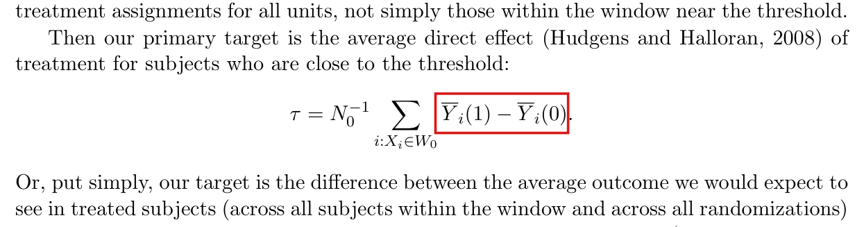
Then our primary target is the average direct effect (Hudgens and Halloran, 2008) of treatment for subjects who are close to the threshold:

τ=N0−1∑i:Xi∈W0Y‾i(1)−Y‾i(0).\tau=N_0^{-1}\sum_{i:X_i\in W_0}\overline{Y}_i(1)-\overline{Y}_i(0).

…

Formally, the difference-in-means estimator for subjects local to the threshold,

τ^=∑i:Xi∈W0YiZi∑i:Xi∈W0Zi−∑i:Xi∈W0Yi(1−Zi)∑i:Xi∈W0(1−Zi).\hat\tau=\frac{\sum_{i:X_i\in W_0}Y_iZ_i}{\sum_{i:X_i\in W_0}Z_i}-\frac{\sum_{i:X_i\in W_0}Y_i(1-Z_i)}{\sum_{i:X_i\in W_0}(1-Z_i)}.

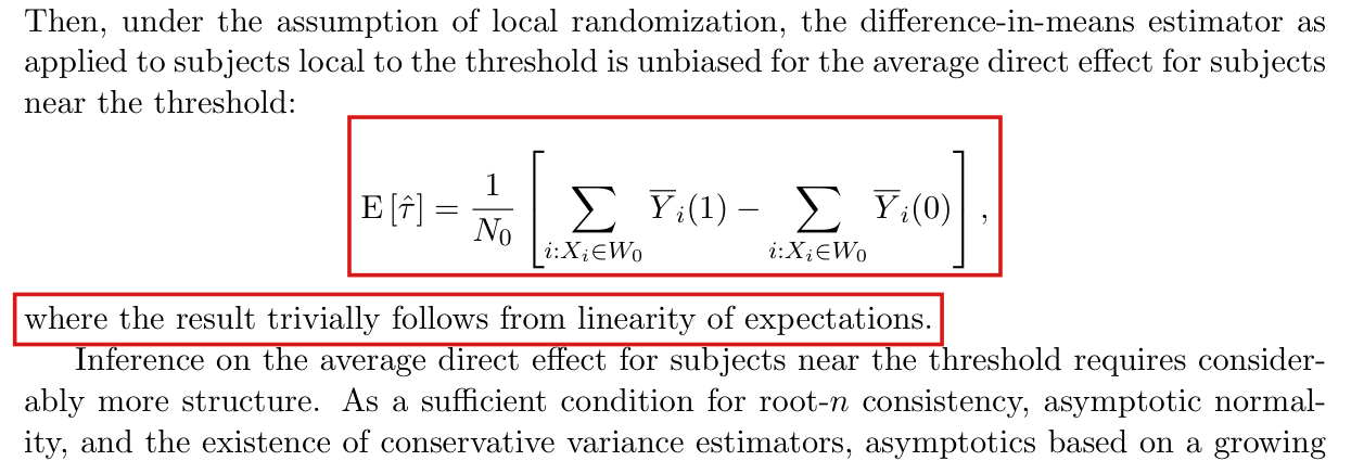
Then, under the assumption of local randomization, the difference-in-means estimator as applied to subjects local to the threshold is unbiased for the average direct effect for subjects near the threshold:

E[τ^]=1N0[∑i:Xi∈W0Y‾i(1)−∑i:Xi∈W0Y‾i(0)],\mathrm{E}[\hat\tau]=\frac{1}{N_0}\Biggl[\sum_{i:X_i\in W_0}\colorbox{#ffe58a}{$\displaystyle \overline{Y}_i(1)$}-\sum_{i:X_i\in W_0}\colorbox{#ffe58a}{$\displaystyle \overline{Y}_i(0)$}\Biggr],

where the result trivially follows from linearity of expectations.

The problem

The first display defines Y‾i(z)\overline{Y}_i(z) as an average of yi(z)y_i(\mathbf{z}) over the distinct assignment vectors in Supp⁡(Z)\operatorname{Supp}(\mathbf{Z}) whose iith component is zz. Each such vector counts once, whatever its probability. The expectation of the difference-in-means estimator weights each assignment vector by its probability. Under local randomization, by linearity of expectation, I have

E[τ^]=1N0∑i:Xi∈W0{E[yi(Z)∣Zi=1]−E[yi(Z)∣Zi=0]}.\mathrm{E}[\hat\tau]=\frac{1}{N_0}\sum_{i:X_i\in W_0}\bigl\{\mathrm{E}[y_i(\mathbf{Z})\mid Z_i=1]-\mathrm{E}[y_i(\mathbf{Z})\mid Z_i=0]\bigr\}.

This equals the printed target for all potential outcomes only if, for each subject ii in the window and each zz, the conditional distribution of Z\mathbf{Z} given Zi=zZ_i=z is uniform on its support. Local randomization does not imply this. Under it the arrangements of the running variable in the window are equiprobable, so that the subjects in the window have equal probabilities of treatment. However, the allocation outside the window is “left completely unspecified”, and the number of arrangements that produce a particular assignment vector of the whole population can vary from one vector to another. The distinct assignment vectors can then have unequal probabilities, so the identity E[τ^]=τ\mathrm{E}[\hat\tau]=\tau need not hold for the printed τ\tau and cannot be justified by linearity of expectations alone.

The prose around the displays describes the probability-weighted quantity: the target is “the average outcome we would expect to see in treated subjects (across all subjects within the window and across all randomizations)” minus the same for control subjects. The display can disagree with the prose when assignment vectors have unequal probabilities, and the text does not settle whether the probabilities were omitted from the display or an assumption of uniform assignment was intended. To keep the allocation outside the window unrestricted, the correction inserts Pr⁡(Z=z)\Pr(\mathbf{Z}=\mathbf{z}) in both sums of the first display. The estimator is unchanged and the estimand changes.

Evidence an exact counterexample

The evidence is two exact counterexamples to the printed identity, and a derivation of the corrected one.

The first example. Let N=4N=4, b=2b=2 and W0=[−2,2]W_0=[-2,2]. Let (X1,X2,X3)(X_1,X_2,X_3) be a uniformly random arrangement of the values −2-2, −1-1 and 11, and set X4=3X_4=3 if (X1,X2,X3)=(−2,−1,1)(X_1,X_2,X_3)=(-2,-1,1) and X4=−3X_4=-3 otherwise. The vector X\mathbf{X} has six support points, each of probability 1/6=1/N0!1/6=1/N_0!. Subjects 1, 2 and 3 are always in the window and subject 4 never is, the values in the window are distinct and the same in every case, and exactly one subject in the window is treated. Every condition printed on p. 130 holds, with the no-ties condition read for distinct subjects (P014-E003), and in addition all six arrangements are equiprobable. Each subject in the window is treated with probability 1/31/3. For all sixteen assignment vectors z\mathbf{z}, set y1(z)=y2(z)=y3(z)=z4y_1(\mathbf{z})=y_2(\mathbf{z})=y_3(\mathbf{z})=z_4 and y4(z)=0y_4(\mathbf{z})=0.

The first example: the four distinct assignment vectors z=(z1,z2,z3,z4)\mathbf{z}=(z_1,z_2,z_3,z_4). The second column counts the arrangements of the running variable that produce z\mathbf{z}; each arrangement has probability 1/61/6. The fourth column is the outcome of subjects 1, 2 and 3.
z\mathbf{z}ArrangementsPr⁡(Z=z)\Pr(\mathbf{Z}=\mathbf{z})yi(z)=z4y_i(\mathbf{z})=z_4τ^\hat\tau
(0,0,1,0)(0,0,1,0)11/61/600
(0,0,1,1)(0,0,1,1)11/61/610
(0,1,0,0)(0,1,0,0)21/31/300
(1,0,0,0)(1,0,0,0)21/31/300

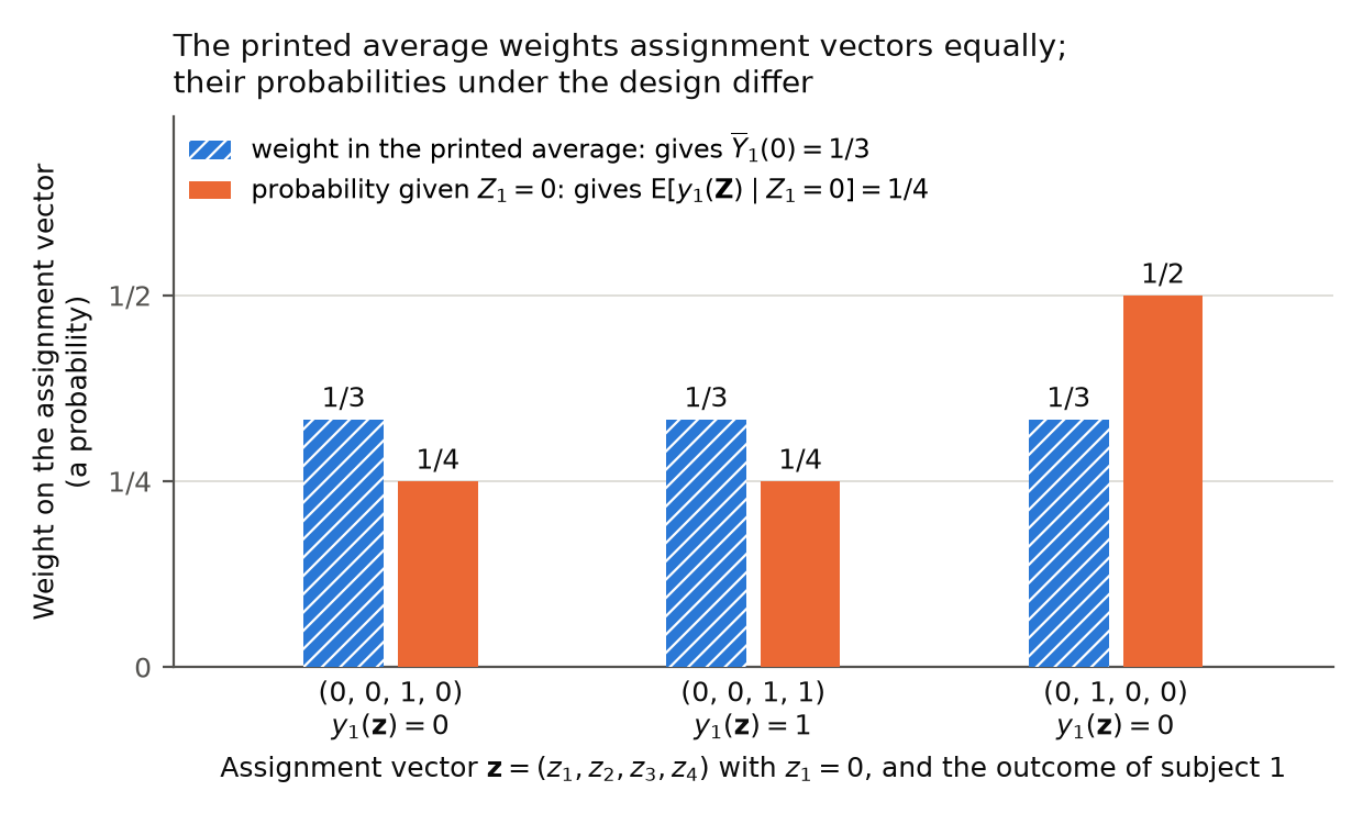
The three subjects in the window always have the same outcome, so that τ^=0\hat\tau=0 for every assignment and E[τ^]=0\mathrm{E}[\hat\tau]=0. The printed Y‾i(z)\overline{Y}_i(z) counts each row of the table once. For subject 1 under control, the rows with z1=0z_1=0 are the first three, with outcomes 00, 11 and 00, and the printed average is 1/31/3. Given Z1=0Z_1=0, these rows have probabilities 1/41/4, 1/41/4 and 1/21/2, and the conditional expectation is 1/41/4.

The first example: the individual average potential outcomes under the printed definition and under the probability-weighted definition.
Subject iiPrinted Y‾i(1)\overline{Y}_i(1)Printed Y‾i(0)\overline{Y}_i(0)E[yi(Z)∣Zi=1]\mathrm{E}[y_i(\mathbf{Z})\mid Z_i=1]E[yi(Z)∣Zi=0]\mathrm{E}[y_i(\mathbf{Z})\mid Z_i=0]
101/31/301/41/4
201/31/301/41/4
31/21/201/21/20

From the second and third columns, I obtain the printed target, and from the last two the probability-weighted target:

τ=13(−13−13+12)=−118,13(−14−14+12)=0=E[τ^].\tau=\frac13\Bigl(-\frac13-\frac13+\frac12\Bigr)=-\frac{1}{18}, \qquad \frac13\Bigl(-\frac14-\frac14+\frac12\Bigr)=0=\mathrm{E}[\hat\tau].

The printed identity fails by 1/181/18.

The second example. Let N=4N=4, b=3b=3 and W0=[−3,3]W_0=[-3,3]. Let (X1,X2,X3)(X_1,X_2,X_3) be a uniformly random arrangement of −1-1, 11 and 22, so that two subjects in the window are treated, and set X4=4X_4=4 if (X1,X2,X3)=(−1,1,2)(X_1,X_2,X_3)=(-1,1,2) and X4=−4X_4=-4 otherwise. Set y2(z)=12z2z4y_2(\mathbf{z})=12z_2z_4 and all other potential outcomes equal to zero. The same conditions hold. The assignment vectors (0,1,1,0)(0,1,1,0) and (0,1,1,1)(0,1,1,1) have probability 1/61/6 each, and (1,0,1,0)(1,0,1,0) and (1,1,0,0)(1,1,0,0) have probability 1/31/3 each. The estimator equals 66 at (0,1,1,1)(0,1,1,1) and 00 elsewhere, so that E[τ^]=1\mathrm{E}[\hat\tau]=1. The printed Y‾2(1)\overline{Y}_2(1) is (0+12+0)/3=4(0+12+0)/3=4, and I find τ=4/3\tau=4/3. The conditional expectation E[y2(Z)∣Z2=1]\mathrm{E}[y_2(\mathbf{Z})\mid Z_2=1] is 33, and the probability-weighted target is 11.

The two exact examples. In each, the six arrangements of the running variable in the window are equiprobable and the conditions printed on p. 130 hold, with the no-ties condition read for distinct subjects.
ExamplePrinted τ\tauE[τ^]\mathrm{E}[\hat\tau]Probability-weighted target
First−1/18-1/1800
Second4/34/311

The corrected identity. Let SS be the set of subjects in the window and n=N0n=N_0. Suppose that ∑i∈SZi=m\sum_{i\in S}Z_i=m with probability one, where 0<m<n0<m<n, and that Pr⁡(Zi=1)=m/n\Pr(Z_i=1)=m/n for every i∈Si\in S. Both hold when the nn distinct values in the window, of which mm are nonnegative, are arranged uniformly at random: a subject receives each value in (n−1)!(n-1)! of the n!n! arrangements. I write p(z)=Pr⁡(Z=z)p(\mathbf{z})=\Pr(\mathbf{Z}=\mathbf{z}) and

Y‾i(a)=∑zp(z) yi(z) I(zi=a)∑zp(z) I(zi=a)=E[yi(Z)∣Zi=a],a∈{0,1}.\overline{Y}_i(a)=\frac{\sum_{\mathbf{z}}p(\mathbf{z})\,y_i(\mathbf{z})\,\mathrm{I}(z_i=a)}{\sum_{\mathbf{z}}p(\mathbf{z})\,\mathrm{I}(z_i=a)}=\mathrm{E}[y_i(\mathbf{Z})\mid Z_i=a],\qquad a\in\{0,1\}.

Since the numbers of treated and control subjects in the window are fixed, I may write

τ^=1m∑i∈Syi(Z)Zi−1n−m∑i∈Syi(Z)(1−Zi).\hat\tau=\frac1m\sum_{i\in S}y_i(\mathbf{Z})Z_i-\frac{1}{n-m}\sum_{i\in S}y_i(\mathbf{Z})(1-Z_i).

For each i∈Si\in S, by the definition of Y‾i(a)\overline{Y}_i(a) and the identity Pr⁡(Zi=1)=m/n\Pr(Z_i=1)=m/n, I have

E[yi(Z)Zi]=∑zp(z) yi(z) I(zi=1)=mn Y‾i(1),E[yi(Z)(1−Zi)]=n−mn Y‾i(0).\mathrm{E}[y_i(\mathbf{Z})Z_i]=\sum_{\mathbf{z}}p(\mathbf{z})\,y_i(\mathbf{z})\,\mathrm{I}(z_i=1)=\frac{m}{n}\,\overline{Y}_i(1), \qquad \mathrm{E}[y_i(\mathbf{Z})(1-Z_i)]=\frac{n-m}{n}\,\overline{Y}_i(0).

Substituting these into the expectation of the previous display, I obtain

E[τ^]=1n∑i∈S{Y‾i(1)−Y‾i(0)}.\mathrm{E}[\hat\tau]=\frac1n\sum_{i\in S}\bigl\{\overline{Y}_i(1)-\overline{Y}_i(0)\bigr\}.

Note that this derivation uses no assumption on the allocation outside the window. In both examples the difference between E[τ^]\mathrm{E}[\hat\tau] and the probability-weighted target vanishes identically as a linear form in the 48 potential outcomes of the three subjects in the window, and the difference between E[τ^]\mathrm{E}[\hat\tau] and the printed target does not.

When the printed target is correct. If Z\mathbf{Z} is uniform on Supp⁡(Z)\operatorname{Supp}(\mathbf{Z}), then the two definitions of Y‾i(z)\overline{Y}_i(z) agree. This is the case when the assignments outside the window are fixed, since each assignment vector is then produced by exactly m!(n−m)!m!(n-m)! arrangements. With X4X_4 fixed in either example, the printed identity holds for all potential outcomes. The two definitions also agree when there is no interference, since yi(z)y_i(\mathbf{z}) then depends on ziz_i alone.

What survives

The difference-in-means estimator, the potential-outcome model with arbitrary interference and the local randomization design are unchanged. The estimator is exactly unbiased for the probability-weighted target with no restriction on the allocation outside the window. This implies that the statement of the Introduction, that it is unbiased for a regime-specific causal effect, holds for that target. The printed target and identity hold as printed when Z\mathbf{Z} is uniform on its support, and when there is no interference. The definition of the estimand changes; in the first example its value changes from −1/18-1/18 to 00. The paper reports no simulations, application or numerical results that depend on the definition. The paragraph on inference on pp. 131–132 refers to the same target, and its sufficient conditions were not examined for this correction.

Corrected

Let S={i:Xi∈W0}S=\{i:X_i\in W_0\} be the fixed set of subjects in the window and n=N0n=N_0. Assume local randomization: the nn distinct, fixed values of the running variable in the window, of which mm are nonnegative with 0<m<n0<m<n, are arranged among the subjects in SS uniformly at random, so that ∑i∈SZi=m\sum_{i\in S}Z_i=m with probability one and Pr⁡(Zi=1)=m/n\Pr(Z_i=1)=m/n for every i∈Si\in S. The allocation outside the window is not restricted. The potential outcomes yi(z)y_i(\mathbf{z}) are fixed and may depend on the whole assignment vector. Denote the individual average potential outcome under treatment zz for all subjects i:Xi∈W0i:X_i\in W_0,

Y‾i(z)=∑z∈Supp⁡(Z)yi(z)I(zi=z) Pr⁡(Z=z)∑z∈Supp⁡(Z)I(zi=z) Pr⁡(Z=z)=E[yi(Z)∣Zi=z].\overline{Y}_i(z)=\frac{\sum_{\mathbf{z}\in\operatorname{Supp}(\mathbf{Z})}y_i(\mathbf{z})\mathrm{I}(\mathbf{z}_i=z)\,\colorbox{#ffe58a}{$\displaystyle \Pr(\mathbf{Z}=\mathbf{z})$}}{\sum_{\mathbf{z}\in\operatorname{Supp}(\mathbf{Z})}\mathrm{I}(\mathbf{z}_i=z)\,\colorbox{#ffe58a}{$\displaystyle \Pr(\mathbf{Z}=\mathbf{z})$}}\colorbox{#ffe58a}{$\displaystyle =\mathrm{E}[y_i(\mathbf{Z})\mid Z_i=z]$}.

Then our primary target is the average direct effect (Hudgens and Halloran, 2008) of treatment for subjects who are close to the threshold:

τ=N0−1∑i:Xi∈W0[Y‾i(1)−Y‾i(0)].\tau=N_0^{-1}\sum_{i:X_i\in W_0}\bigl[\overline{Y}_i(1)-\overline{Y}_i(0)\bigr].

The difference-in-means estimator τ^\hat\tau is as printed. Then, under the assumption of local randomization, the difference-in-means estimator as applied to subjects local to the threshold is unbiased for the average direct effect for subjects near the threshold:

E[τ^]=1N0[∑i:Xi∈W0Y‾i(1)−∑i:Xi∈W0Y‾i(0)],\mathrm{E}[\hat\tau]=\frac{1}{N_0}\Biggl[\sum_{i:X_i\in W_0}\overline{Y}_i(1)-\sum_{i:X_i\in W_0}\overline{Y}_i(0)\Biggr],

where the result follows from the fixed numbers of treated and control subjects in the window, their common probability of treatment, and linearity of expectations. The brackets in the display for τ\tau are those of P014-N004. The treated-minus-control contrast uses the reverse of Hudgens and Halloran’s sign convention (P014-N002).

Alternatively, the definition of Y‾i(z)\overline{Y}_i(z) printed on p. 131 can be kept under the additional assumption that Z\mathbf{Z} is uniformly distributed on Supp⁡(Z)\operatorname{Supp}(\mathbf{Z}), which holds, for instance, when the assignments of the subjects outside the window are fixed. The two definitions then agree.
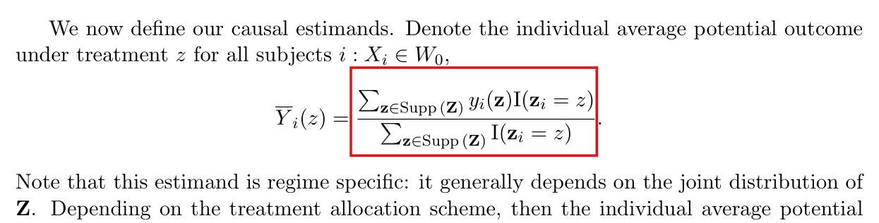
Two lines of text introduce the individual average potential outcome under treatment z, followed by a display. A red box marks the fraction that defines Y-bar i of z. Its numerator is the sum over z in Supp(Z) of y i of z times the indicator that z i equals z, and its denominator is the sum over z in Supp(Z) of that indicator. Two lines below the display begin 'Note that this estimand is regime specific'.
Section 2, first display, p. 131 (PDF p. 4). The marked fraction defines Y‾i(z)\overline{Y}_i(z) as an average over the assignment vectors in Supp⁡(Z)\operatorname{Supp}(\mathbf{Z}). No probability appears in either sum.
Three lines of text say that under local randomization the difference-in-means estimator is unbiased for the average direct effect for subjects near the threshold. A red box marks the display 'E of tau-hat equals one over N0 times, in square brackets, the sum over i with Xi in W0 of Y-bar i of 1 minus the sum over i with Xi in W0 of Y-bar i of 0'. A second red box marks the sentence 'where the result trivially follows from linearity of expectations.' Three lines of the next paragraph, on inference, follow.
Section 2, p. 131 (PDF p. 4). The marked display equates E[τ^]\mathrm{E}[\hat\tau] with the target built from the printed Y‾i(z)\overline{Y}_i(z), and the marked sentence attributes the identity to linearity of expectations.
Bar chart with three groups, one for each assignment vector with z1 equal to 0. The groups are (0, 0, 1, 0), where the outcome of subject 1 is 0; (0, 0, 1, 1), where it is 1; and (0, 1, 0, 0), where it is 0. In each group a hatched blue bar shows the weight in the printed average, which is 1/3 in all three groups, and an orange bar shows the probability given Z1 equal to 0, which is 1/4, 1/4 and 1/2. The legend says that the printed weights give Y-bar 1 of 0 equal to 1/3 and that the probabilities give the conditional expectation 1/4. The title reads 'The printed average weights assignment vectors equally; their probabilities under the design differ'.
The first example, subject 1 under control. The printed Y‾1(0)\overline{Y}_1(0) assigns weight 1/31/3 to each of the three assignment vectors with z1=0z_1=0 and equals 1/31/3. Given Z1=0Z_1=0, these vectors have probabilities 1/41/4, 1/41/4 and 1/21/2 under the design, and the expected outcome is 1/41/4. All values are exact.
My comment and the history of this entry

Agreed.

  1. Classification before my review (the classification when the audit was first completed, before I reviewed it): Moderate error.
  2. I commented.
  3. Independent evaluation. No change was needed: my comment agrees with the entry.

Minor (6)

Real but inconsequential, for example a misprint that does not change a result.

The probability condition in the local randomization assumption should be placed on the running variables of the subjects in the window, Pr⁡(XS=a)=1/N0!\Pr(\mathbf{X}_S=a)=1/N_0! for every arrangement aa of their values, and not on the full vector X\mathbf{X}.

Section 2, final paragraph, p. 130 (PDF p. 3), sentence beginning “Our local randomization assumption requires that”; related sentence on p. 131 (PDF p. 4), beginning “While the treatment allocation scheme”

See also under Formal statements (Lean): P014-T2, P014-T3, P014-T5, P014-T6, P014-T7

As printed

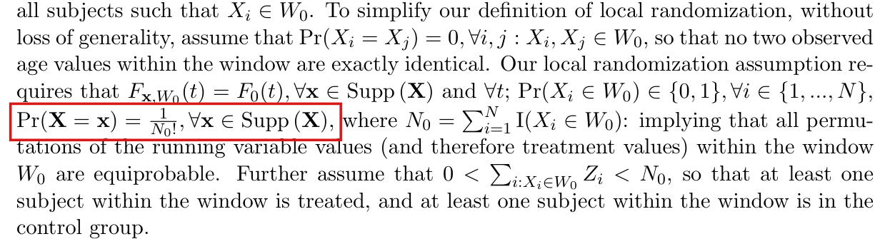
Our local randomization assumption requires that Fx,W0(t)=F0(t)F_{\mathbf{x},W_0}(t)=F_0(t), ∀x∈Supp⁡(X)\forall\mathbf{x}\in\operatorname{Supp}(\mathbf{X}) and ∀t\forall t; Pr⁡(Xi∈W0)∈{0,1}\Pr(X_i\in W_0)\in\{0,1\}, ∀i∈{1,…,N}\forall i\in\{1,\ldots,N\}, Pr⁡(X=x)=1N0!\Pr(\colorbox{#ffe58a}{$\mathbf{X}=\mathbf{x}$})=\frac{1}{N_0!}, ∀x∈Supp⁡(X)\forall\colorbox{#ffe58a}{$\mathbf{x}\in\operatorname{Supp}(\mathbf{X})$}, where N0=∑i=1NI(Xi∈W0)N_0=\sum_{i=1}^{N}\mathrm{I}(X_i\in W_0): implying that all permutations of the running variable values (and therefore treatment values) within the window W0W_0 are equiprobable. Further assume that 0<∑i:Xi∈W0Zi<N00<\sum_{i:X_i\in W_0}Z_i<N_0, so that at least one subject within the window is treated, and at least one subject within the window is in the control group.

The problem

Under the marked clause, every support point of the full vector X=(X1,…,XN)\mathbf{X}=(X_1,\ldots,X_N) has probability 1/N0!1/N_0!. The sentence then says that its clauses imply that all permutations of the running variable values within the window are equiprobable. They do not. I define an arrangement to be an assignment of the N0N_0 values in the window to the N0N_0 subjects in the window. Two support points of X\mathbf{X} can have the same arrangement and differ outside the window. The clauses fix the number of support points at N0!N_0!, but they do not fix how many support points have a given arrangement. Some arrangements can have probability zero and others probability above 1/N0!1/N_0!, and the subjects in the window can then have unequal probabilities of treatment.

The clause is also too strong once the conclusion drawn from it is granted. If the N0!N_0! arrangements are equiprobable and every support point of X\mathbf{X} has probability 1/N0!1/N_0!, then the running variables outside the window are a function of the arrangement. An allocation outside the window that remains random given the arrangement is excluded, although p. 131 says that this allocation is “left completely unspecified”. The words after the colon state the intended assumption, which is a uniformly random arrangement, and the correction states that assumption directly.

Evidence an exact counterexample

The evidence is an exact counterexample to the implication, together with a counting argument for the corrected condition.

The counterexample. Let N=4N=4, b=2b=2 and W0=[−2,2]W_0=[-2,2], and assign probability 1/61/6 to each of the six vectors

(1,−1,−2,3),(−1,1,−2,3),(−1,−2,1,3),(−1,−2,1,4),(−1,−2,1,5),(−1,−2,1,6).(1,-1,-2,3),\quad (-1,1,-2,3),\quad (-1,-2,1,3),\quad (-1,-2,1,4),\quad (-1,-2,1,5),\quad (-1,-2,1,6).

Subjects 1, 2 and 3 are in the window with probability one and subject 4 is never in it, so that N0=3N_0=3. In each vector the values in the window are −2-2, −1-1 and 11. They are distinct, and the empirical distribution function Fx,W0F_{\mathbf{x},W_0} is the same for all six. Each support point has probability 1/6=1/N0!1/6=1/N_0!, and exactly one subject in the window is treated. Every printed clause holds. However, the arrangement (−1,−2,1)(-1,-2,1) has probability 2/32/3, the arrangements (1,−1,−2)(1,-1,-2) and (−1,1,−2)(-1,1,-2) have probability 1/61/6 each, and the other three have probability zero. Subjects 1, 2 and 3 are treated with probabilities 1/61/6, 1/61/6 and 2/32/3. Let y1(z)=z1y_1(\mathbf{z})=z_1, and let all other potential outcomes be zero, so that there is no interference. Then τ=1/3\tau=1/3, while τ^=Z1\hat\tau=Z_1 and E[τ^]=1/6\mathrm{E}[\hat\tau]=1/6.

The counting argument. Let SS be the set of subjects in the window, write n=N0n=N_0, and let XS=(Xi)i∈S\mathbf{X}_S=(X_i)_{i\in S}. For an arrangement aa, let k(a)k(a) be the number of support points x\mathbf{x} of X\mathbf{X} such that xS=a\mathbf{x}_S=a. Under the printed clauses, I have Pr⁡(XS=a)=k(a)/n!\Pr(\mathbf{X}_S=a)=k(a)/n!, and nothing determines k(a)k(a). If in addition Pr⁡(XS=a)=1/n!\Pr(\mathbf{X}_S=a)=1/n! for every aa, then k(a)=1k(a)=1 for every aa, so that the values outside the window are a function of XS\mathbf{X}_S. For instance, let the arrangement be uniform over the six arrangements of −2-2, −1-1 and 11, and let X4X_4 be independent of it, equal to −3-3 with probability 1/31/3 and to 33 with probability 2/32/3. Then X\mathbf{X} has twelve support points, with probabilities 1/181/18 and 1/91/9, and none has probability 1/61/6. Under the corrected condition, let mm be the number of nonnegative values in the window. A subject i∈Si\in S receives a nonnegative value in m(n−1)!m(n-1)! of the n!n! arrangements, which implies that Pr⁡(Zi=1)=m/n\Pr(Z_i=1)=m/n.

What survives

The potential-outcome model, the threshold rule that sets Zi=1Z_i=1 when Xi≥0X_i\ge 0, the fixed set of subjects in the window and the difference-in-means estimator are unchanged. The corrected condition is the assumption that the prose of the sentence already states, and it changes neither the estimator nor the intended estimand. Under it every subject in the window is treated with probability m/nm/n, and without interference the unbiasedness argument on p. 131 holds as printed. This correction does not repair the definition of the target under interference, which is the subject of P014-E001.

Corrected

Let S={i:Pr⁡(Xi∈W0)=1}S=\{i:\Pr(X_i\in W_0)=1\} be the set of subjects in the window, and let n=N0n=N_0 be its size. Our local randomization assumption requires that Pr⁡(Xi∈W0)∈{0,1}\Pr(X_i\in W_0)\in\{0,1\}, ∀i∈{1,…,N}\forall i\in\{1,\ldots,N\}; that Fx,W0(t)=F0(t)F_{\mathbf{x},W_0}(t)=F_0(t), ∀x∈Supp⁡(X)\forall\mathbf{x}\in\operatorname{Supp}(\mathbf{X}) and ∀t\forall t, where F0F_0 is the empirical distribution function of nn distinct values v1,…,vnv_1,\ldots,v_n; and that

Pr⁡(XS=a)=1n!for every arrangement a of v1,…,vn among the subjects in S,\Pr(\colorbox{#ffe58a}{$\displaystyle \mathbf{X}_S=a$})=\frac{1}{n!}\quad\text{for every arrangement } \colorbox{#ffe58a}{$\displaystyle a$} \text{ of } v_1,\ldots,v_n \text{ among the subjects in } S,

where XS=(Xi)i∈S\mathbf{X}_S=(X_i)_{i\in S}. That is, all permutations of the running variable values (and therefore treatment values) within the window W0W_0 are equiprobable. The distribution of the running variables outside the window, given XS\mathbf{X}_S, is restricted only by Pr⁡(Xi∈W0)=0\Pr(X_i\in W_0)=0 for i∉Si\notin S, and it need not be independent of XS\mathbf{X}_S. Further assume that the number mm of nonnegative values among v1,…,vnv_1,\ldots,v_n satisfies 0<m<n0<m<n, so that at least one subject within the window is treated, and at least one subject within the window is in the control group. Then ∑i∈SZi=m\sum_{i\in S}Z_i=m with probability one, and Pr⁡(Zi=1)=m/n\Pr(Z_i=1)=m/n for every i∈Si\in S.

Nine lines of text from the final paragraph of Section 2. A red box marks the clause 'Pr(X = x) = 1/N0!, for all x in Supp(X)', with X and x in bold. The line continues 'where N0 is the sum of the indicators that Xi is in W0: implying that all permutations of the running variable values (and therefore treatment values) within the window W0 are equiprobable'.
Section 2, final paragraph, p. 130 (PDF p. 3). The marked clause assigns probability 1/N0!1/N_0! to each support point of the full vector X\mathbf{X}. The words after the colon draw the conclusion that the permutations within the window are equiprobable.

The no-ties condition should be restricted to distinct subjects: Pr⁡(Xi=Xj)=0\Pr(X_i=X_j)=0 for all i≠ji\neq j such that Xi,Xj∈W0X_i,X_j\in W_0.

Section 2, final paragraph, p. 130 (PDF p. 3), sentence beginning “To simplify our definition of local randomization”

See also under Formal statements (Lean): P014-T1, P014-T4, P014-T5, P014-T7, P014-T9

As printed

To simplify our definition of local randomization, without loss of generality, assume that Pr⁡(Xi=Xj)=0, ∀i,j:Xi,Xj∈W0\Pr(X_i=X_j)=0,\ \colorbox{#ffe58a}{$\forall i,j$}:X_i,X_j\in W_0, so that no two observed age values within the window are exactly identical.

The problem

The quantifier ranges over all pairs i,ji,j of subjects in the window, including j=ij=i. Since Pr⁡(Xi=Xi)=1\Pr(X_i=X_i)=1, the condition cannot hold as printed. The words that follow it, “no two observed age values”, state the intended condition, which concerns distinct subjects.

Evidence a derivation

The evidence is a check of the page and a one-line derivation. No restriction i≠ji\neq j is printed. The window contains at least one subject, since the same paragraph assumes 0<∑i:Xi∈W0Zi<N00<\sum_{i:X_i\in W_0}Z_i<N_0. For such a subject ii, the printed condition with j=ij=i requires Pr⁡(Xi=Xi)=0\Pr(X_i=X_i)=0, while the event {Xi=Xi}\{X_i=X_i\} has probability one.

What survives

Adding i≠ji\neq j expresses the intended no-ties condition without changing the intended local randomization design. I did not examine whether “without loss of generality” is justified for every model of the running variable.

Corrected

To simplify our definition of local randomization, without loss of generality, assume that Pr⁡(Xi=Xj)=0, ∀i,j:i≠j, Xi,Xj∈W0\Pr(X_i=X_j)=0,\ \forall i,j:\colorbox{#ffe58a}{$i\neq j$},\ X_i,X_j\in W_0, so that no two observed age values within the window are exactly identical.

Three lines of text. A red box marks the formula 'Pr(Xi = Xj) = 0, for all i, j : Xi, Xj in W0'. It is followed by the words 'so that no two observed age values within the window are exactly identical'.
Section 2, final paragraph, p. 130 (PDF p. 3). The marked condition is quantified over all i,ji,j such that Xi,Xj∈W0X_i,X_j\in W_0, with no restriction to i≠ji\neq j.

Six entries of the reference list contain misprints: a misspelled surname, a repeated word, three closing quotation marks without an opening mark, and a Neyman entry that prints its title twice and sets a fragment of the author’s name among the translators.

References, pp. 132–133 (PDF pp. 5–6): the entries Cattaneo, Frandsen and Titiunik (2015) and Cattaneo, Titiunik and Vasquez-Bare (2016) on p. 132; Lee (2008), Neyman (1923), Rosenbaum (2007), and Thistlethwaite and Campbell (1960) on p. 133

As printed
  • Cattaneo, M.D., B.R. Frandsen, and R. Titiunik (2015). Randomization inference in the regression discontinuity design: an application to party advantages in the U.S. Senate.” Journal of Causal Inference. 3(1): 1 –24.
  • Cattaneo, M.D., R. Titiunik, and G. Vasquez-Bare (2016). Inference in regression discontinuity designs under local randomization. The Stata Journal. 16(2): 331 – 367.
  • Lee, D. (2008) Randomized experiments from non-random selection in U.S. House elections.” Journal of Econometrics. 142: 675 – 697.
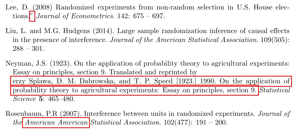
  • Neyman, J.S. (1923). On the application of probability theory to agricultural experiments: Essay on principles, section 9. Translated and reprinted by erzy Splawa, D. M. Dabrowska, and T. P. Speed [1923.] 1990. On the application of probability theory to agricultural experiments: Essay on principles, section 9. Statistical Science 5: 465–480.
  • Rosenbaum, P.R (2007). Interference between units in randomized experiments. Journal of the American American Statistical Association. 102(477): 191 – 200.
  • Thistlethwaite, D. and D. Campbell. (1960). Regression-discontinuity analysis: an alternative to the ex post facto experiment.” Journal of Educational Psychology. 51: 309 – 317.
The problem

The surname in the 2016 entry is spelled “Vasquez-Bare”, while the text on pp. 129 and 132 has “Vazquez-Bare”, which is the spelling of the journal’s byline. The Rosenbaum entry prints “American” twice. Three titles end with a closing quotation mark that has no opening mark. The Neyman entry runs two citations of one item together. Its title is printed twice, the date appears as “[1923.] 1990”, and “erzy Splawa”, a fragment of the author’s name Jerzy Splawa-Neyman, stands among the translators. The page range 465–480 of that entry is not an error: it is the range on the masthead of the translation, which covers the translation (465–472) and the discussion that follows it.

Evidence a check of the printed page

The evidence is a check of the pages against public sources. The article page of The Stata Journal names the third author as Gonzalo Vazquez-Bare. The title page of the 1990 translation in Statistical Science names the author as Jerzy Splawa-Neyman, carries the credit “Translated and edited by D. M. Dabrowska and T. P. Speed”, and has the masthead “1990, Vol. 5, No. 4, 465-480”. The contents of that issue list the comment by D. B. Rubin separately at pp. 472–480.

What survives

Every cited work remains identifiable, and no mathematical content or result of the paper is affected.

Corrected
  • Cattaneo, M.D., B.R. Frandsen, and R. Titiunik (2015). Randomization inference in the regression discontinuity design: an application to party advantages in the U.S. Senate. Journal of Causal Inference. 3(1): 1 –24.
  • Cattaneo, M.D., R. Titiunik, and G. Vazquez-Bare (2016). Inference in regression discontinuity designs under local randomization. The Stata Journal. 16(2): 331 – 367.
  • Lee, D. (2008) Randomized experiments from non-random selection in U.S. House elections. Journal of Econometrics. 142: 675 – 697.
  • Splawa-Neyman, J. (1923 [1990]). On the application of probability theory to agricultural experiments. Essay on principles. Section 9. Translated and edited by D. M. Dabrowska and T. P. Speed. Statistical Science 5(4): 465–472 (with discussion, 465–480).
  • Rosenbaum, P.R (2007). Interference between units in randomized experiments. Journal of the American Statistical Association. 102(477): 191 – 200.
  • Thistlethwaite, D. and D. Campbell. (1960). Regression-discontinuity analysis: an alternative to the ex post facto experiment. Journal of Educational Psychology. 51: 309 – 317.
Two entries of the reference list. In the first, Cattaneo, Frandsen and Titiunik (2015), a red box marks the closing quotation mark after the word Senate at the end of the title. In the second, Cattaneo, Titiunik and Vasquez-Bare (2016), a red box marks the surname Vasquez-Bare, spelled with an s.
References, p. 132 (PDF p. 5). The marks show the closing quotation mark after the title of the Cattaneo, Frandsen and Titiunik entry, which has no opening mark, and the spelling “Vasquez-Bare”.
Four entries of the reference list: Lee (2008), Liu and Hudgens (2014), Neyman (1923) and Rosenbaum (2007). A red box marks the closing quotation mark after 'elections.' in the Lee entry. Two red boxes mark the third and fourth lines of the Neyman entry, which read 'erzy Splawa, D. M. Dabrowska, and T. P. Speed [1923.] 1990. On the application of probability theory to agricultural experiments: Essay on principles, section 9.' A red box marks the words 'American American' in the journal name of the Rosenbaum entry.
References, p. 133 (PDF p. 6). The marks show the unmatched closing quotation mark in the Lee entry; the two lines of the Neyman entry that hold the fragment “erzy Splawa”, the date “[1923.] 1990” and the repeated title; and the repeated word “American” in the Rosenbaum entry.
The three lines of the entry Thistlethwaite and Campbell (1960). A red box marks the closing quotation mark after the word experiment at the end of the title.
References, p. 133 (PDF p. 6). The mark shows the unmatched closing quotation mark in the Thistlethwaite and Campbell entry.

The target is the average direct effect of Hudgens and Halloran (2008) for the subjects in the window once Y‾i(z)\overline{Y}_i(z) is the conditional expectation E[yi(Z)∣Zi=z]\mathrm{E}[y_i(\mathbf{Z})\mid Z_i=z], and then with the opposite sign: their direct effect is control minus treatment.

Introduction, p. 129 (PDF p. 2), sentence beginning “This causal effect is equivalent to”; Section 2, p. 131 (PDF p. 4), sentence beginning “Then our primary target is the average direct effect”

See also under Formal statements (Lean): P014-T7, P014-T9, P014-T10

As printed

Introduction (p. 129). This causal effect is equivalent to Hudgens and Halloran (2008)'s average direct effect for the subpopulation of subjects within the window near the threshold.

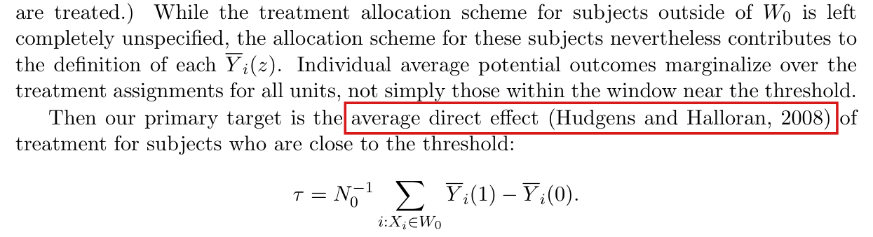
Section 2 (p. 131). Then our primary target is the average direct effect (Hudgens and Halloran, 2008) of treatment for subjects who are close to the threshold:

τ=N0−1∑i:Xi∈W0Y‾i(1)−Y‾i(0).\tau=N_0^{-1}\sum_{i:X_i\in W_0}\overline{Y}_i(1)-\overline{Y}_i(0).
The problem

Hudgens and Halloran (2008) define the individual average potential outcome as a conditional expectation. The outcomes of an individual are averaged over the assignments of the other individuals, each weighted by its conditional probability given the individual’s own treatment. They define the individual direct causal effect as the average under control minus the average under treatment. The target τ\tau differs from the average of that effect over the subjects in the window in two ways. First, the printed Y‾i(z)\overline{Y}_i(z) weights the distinct assignment vectors equally and is not their conditional expectation in general; this is the error corrected in P014-E001. Second, τ\tau is treated minus control. Once the probabilities are inserted, τ\tau is therefore the negative of their average direct effect for the subjects in the window. The sign is a convention. The paper uses treated minus control in both τ\tau and τ^\hat\tau, and no result on estimation depends on it.

Evidence an exact counterexample

The evidence is a reading of the cited paper and an exact example. In the public author manuscript of Hudgens and Halloran (2008), the definition in Section 3.1 multiplies each potential outcome by Pr⁡ψ(Zi(j)=ω∣Zij=z)\Pr_\psi(\mathbf{Z}_{i(j)}=\omega\mid Z_{ij}=z) and is followed by the statement that the “individual average potential outcome is the conditional expectation”. In Section 3.2, equation (3) defines the individual direct causal effect as Y‾ij(0;ψ)−Y‾ij(1;ψ)\overline{Y}_{ij}(0;\psi)-\overline{Y}_{ij}(1;\psi). I did not check the page and equation numbers of the version of record.

For the example, let N=4N=4, b=1b=1 and W0=[−1,1]W_0=[-1,1]. Let (X1,X2,X3)(X_1,X_2,X_3) be a uniformly random arrangement of −1-1, −1/2-1/2 and 1/21/2, and set X4=2X_4=2 if (X1,X2,X3)=(−1,−1/2,1/2)(X_1,X_2,X_3)=(-1,-1/2,1/2) and X4=−2X_4=-2 otherwise. Set y1(z)=z4y_1(\mathbf{z})=z_4 and all other potential outcomes equal to zero. The conditions printed on p. 130 hold and the six arrangements are equiprobable. The assignment vectors (0,0,1,0)(0,0,1,0) and (0,0,1,1)(0,0,1,1) have probability 1/61/6 each, and (0,1,0,0)(0,1,0,0) and (1,0,0,0)(1,0,0,0) have probability 1/31/3 each. The printed Y‾1(0)\overline{Y}_1(0) is 1/31/3, while E[y1(Z)∣Z1=0]=1/4\mathrm{E}[y_1(\mathbf{Z})\mid Z_1=0]=1/4, and all other averages are zero. I obtain

τ=−19,13{E[y1(Z)∣Z1=1]−E[y1(Z)∣Z1=0]}=−112=E[τ^],\tau=-\frac19,\qquad \frac13\bigl\{\mathrm{E}[y_1(\mathbf{Z})\mid Z_1=1]-\mathrm{E}[y_1(\mathbf{Z})\mid Z_1=0]\bigr\}=-\frac{1}{12}=\mathrm{E}[\hat\tau],

and the average direct effect in the convention of Hudgens and Halloran is 1/121/12. The printed τ\tau equals neither 1/121/12 nor −1/12-1/12. To isolate the sign, fix the assignment of subject 4 at control and set yi(z)=ziy_i(\mathbf{z})=z_i for the subjects in the window. Then the two definitions of Y‾i(z)\overline{Y}_i(z) agree, τ=E[τ^]=1\tau=\mathrm{E}[\hat\tau]=1, and the average direct effect in their convention is −1-1.

What survives

The estimator, the design and, with the definition corrected in P014-E001, the unbiasedness of the estimator are unaffected. The reference to Hudgens and Halloran (2008) remains the right one for the probability-weighted target. The identification with their average direct effect needs a remark on the sign.

Corrected

Introduction (p. 129). With the probability-weighted averages of P014-E001, this causal effect is, up to the sign convention, Hudgens and Halloran (2008)'s average direct effect for the subpopulation of subjects within the window near the threshold.

Section 2 (p. 131). With Y‾i(z)=E[yi(Z)∣Zi=z]\overline{Y}_i(z)=\mathrm{E}[y_i(\mathbf{Z})\mid Z_i=z] as in P014-E001, our primary target is the average direct effect (Hudgens and Halloran, 2008) of treatment for subjects who are close to the threshold, written as treated minus control, which is the reverse of their sign convention:

τ=N0−1∑i:Xi∈W0[Y‾i(1)−Y‾i(0)].\tau=N_0^{-1}\sum_{i:X_i\in W_0}\bigl[\overline{Y}_i(1)-\overline{Y}_i(0)\bigr].
Six lines of text followed by a display. A red box marks the words 'average direct effect (Hudgens and Halloran, 2008)' in the sentence 'Then our primary target is the average direct effect (Hudgens and Halloran, 2008) of treatment for subjects who are close to the threshold'. The display reads 'tau equals N0 to the minus 1 times the sum over i with Xi in W0 of Y-bar i of 1 minus Y-bar i of 0'.
Section 2, p. 131 (PDF p. 4). The marked words identify the target with the average direct effect of Hudgens and Halloran (2008). The display below them is treated minus control.
Four lines of text from the end of the Introduction. Red boxes mark the words 'This causal effect is equivalent to Hudgens and Halloran (2008)'s average direct effect', which run over two lines. The sentence continues 'for the subpopulation of subjects within the window near the threshold'.
Introduction, p. 129 (PDF p. 2). The marked sentence says that the causal effect is equivalent to the average direct effect of Hudgens and Halloran (2008).

The summand in the definition of τ\tau should be bracketed: τ=N0−1∑i:Xi∈W0[Y‾i(1)−Y‾i(0)]\tau=N_0^{-1}\sum_{i:X_i\in W_0}[\overline{Y}_i(1)-\overline{Y}_i(0)].

Section 2, p. 131 (PDF p. 4), the display that defines τ\tau

See also under Formal statements (Lean): P014-T4, P014-T8

As printed
τ=N0−1∑i:Xi∈W0Y‾i(1)−Y‾i(0).\tau=N_0^{-1}\sum_{i:X_i\in W_0}\colorbox{#ffe58a}{$\displaystyle \overline{Y}_i(1)-\overline{Y}_i(0)$}.
The problem

The two terms after the summation sign are not bracketed. Read literally, the sum and the factor N0−1N_0^{-1} apply to Y‾i(1)\overline{Y}_i(1) alone, and the index ii in Y‾i(0)\overline{Y}_i(0) is free. The prose that follows, and the display for E[τ^]\mathrm{E}[\hat\tau] on the same page, show that both terms belong to the summand.

Evidence a check of the printed page

The evidence is a check of the page. The display that defines τ\tau has neither brackets nor a second summation sign. The later display reads E[τ^]=N0−1[∑i:Xi∈W0Y‾i(1)−∑i:Xi∈W0Y‾i(0)]\mathrm{E}[\hat\tau]=N_0^{-1}[\sum_{i:X_i\in W_0}\overline{Y}_i(1)-\sum_{i:X_i\in W_0}\overline{Y}_i(0)], and by linearity of the finite sum its right side equals the bracketed form below.

What survives

The intended target and its agreement with the display for E[τ^]\mathrm{E}[\hat\tau] are unaffected, and nothing depends on the missing brackets. The definition of Y‾i(z)\overline{Y}_i(z) inside the sum is corrected separately in P014-E001.

Corrected
τ=N0−1∑i:Xi∈W0[Y‾i(1)−Y‾i(0)].\tau=N_0^{-1}\sum_{i:X_i\in W_0}\colorbox{#ffe58a}{$\displaystyle \bigl[$}\overline{Y}_i(1)-\overline{Y}_i(0)\colorbox{#ffe58a}{$\displaystyle \bigr]$}.
Three lines of text followed by a display and two more lines. The display reads 'tau equals N0 to the minus 1 times the sum over i with Xi in W0 of Y-bar i of 1 minus Y-bar i of 0'. A red box marks the two terms after the summation sign, 'Y-bar i of 1 minus Y-bar i of 0', which are not enclosed in brackets.
Section 2, p. 131 (PDF p. 4), the display that defines τ\tau. The marked summand Y‾i(1)−Y‾i(0)\overline{Y}_i(1)-\overline{Y}_i(0) has no brackets.

The page range of Sobel (2006) is 1398–1407, not 1398–1408.

References, p. 133 (PDF p. 6), the entry Sobel (2006)

As printed

Sobel, M.E. (2006). What do randomized studies of housing mobility demonstrate?: Causal inference in the face of interference. Journal of the American Statistical Association 101 (476): 1398–1408.

The problem

The range is one page too long. Page 1408 of that issue is the first page of the next article.

Evidence a check of the printed page

The evidence is a check against the publisher. Its table of contents for the Journal of the American Statistical Association 101(476) lists Sobel’s article at pages 1398–1407 and the next article, “Exceedance Control of the False Discovery Proportion”, at pages 1408–1417. The publisher’s page for the article has the same range.

What survives

The cited work remains identifiable, and nothing in the paper depends on the last page.

Corrected

Sobel, M.E. (2006). What do randomized studies of housing mobility demonstrate?: Causal inference in the face of interference. Journal of the American Statistical Association 101 (476): 1398–1407.

Two entries of the reference list, Rosenbaum (2007) and Sobel (2006). A red box marks the page range 1398-1408 at the end of the Sobel entry.
References, p. 133 (PDF p. 6). The marked page range of the Sobel (2006) entry ends at 1408.

Formal statements (Lean)

Formal results: 9 whole; 0 restricted; 1 refuted; 0 omitted.

Coverage concerns the identified claim under its stated assumptions. A checked proof establishes the formal statement; correspondence to the published text was reviewed by AI. Repository access is currently required to open the source links.

Each result links to its current formal statement and proof. “Whole” covers the identified claim under its assumptions; “restricted” covers the stated narrower scope; “refuted” gives a counterexample to the identified assertion; “omitted” has no current theorem. Any named published theorem used as a premise remains an assumption. Browse the formal results for this work.

Section 2, the individual average potential outcome, the target τ\tau and the unbiasedness display, corrected: probability-weighted averages, same estimator

p. 131 (PDF p. 4)

p. 131 (PDF p. 4), assumptions p. 130: with a fixed interior treated count and common propensities, probability-weighted own-arm averages are conditional expectations with positive denominators, and the unchanged difference in means is unbiased for their bracketed window contrast. All four displayed derivation steps hold. Corrected uniform local score arrangements imply these hypotheses and this identity for arbitrary potential outcomes, with the outside allocation and its dependence unrestricted.

Historical component credits
  • Proved AronowAudit.P014.expect_map Limited support; baseline fidelity: narrower; manifest: not used; not used in Solution; Narrower row used nowhere: it supplies pushforward change of variables, not standalone linearity; expectation_fixed_counts already exports the required assignment-law linearity calculation.
  • Proved AronowAudit.P014.armCounts_add Historical support retained; baseline fidelity: ok; manifest: used; used in Solution; Auxiliary partition identity, including empty windows; the corrected main theorem separately imposes 0<m<|S|.
  • Proved AronowAudit.P014.armMasses_add Historical support retained; baseline fidelity: ok; manifest: used; used in Solution; No individual positivity premise is needed for this auxiliary complement identity; target A2 later ensures both arm probabilities are positive.
  • Proved AronowAudit.P014.expectation_fixed_counts Historical support retained; baseline fidelity: ok; manifest: used; used in Solution; The saved claim-stage verdict is unchanged. This is a sound algebraic extension to empty arms using a/0=0, and specialization to the target's 0<m<n is exact. Calling this broader_than_claim is a classification difference from the earlier faithful_with_notes verdict, not a mathematical objection.
  • Proved AronowAudit.P014.moment_identity Historical support retained; baseline fidelity: ok; manifest: used; used in Solution; The nonzero premise is already implied by A2 and 0<m<n for either arm; it therefore excludes no target case. The corrected conditional mean is its finite weighted ratio.
  • Proved AronowAudit.P014.weighted_unbiasedness Historical support retained; baseline fidelity: ok; manifest: used; used in Solution; All hypotheses match A1, A2 and 0<m<n; finite-support equality is equivalent to almost-sure equality for binary assignments. This row proves the corrected identity under those conditions, while the target's separate corrected-score-randomization application is not established by the credited rows read here.
  • Proved AronowAudit.P014.prob_map Historical support retained; baseline fidelity: ok; manifest: not used; not used in Solution; Not separately invoked; the score-to-assignment application is omitted from T2.
  • Proved AronowAudit.P014.armMass_as_prob Historical support retained; baseline fidelity: ok; manifest: used; used in Solution; The finite-support representation loses no binary-assignment law because the population is finite. The mass function outside the chosen support is irrelevant to every arm probability.
  • Proved AronowAudit.P014.mem_map_support_iff Historical support retained; baseline fidelity: ok; manifest: used; used in Solution; Not separately invoked; the retained assignment-law statement does not construct a law from running scores.

Section 2, the display defining the target τ\tau, corrected: the summand bracketed

p. 131 (PDF p. 4)

p. 131 (PDF p. 4): the bracketed window mean of differences is the difference of the two sums divided by the nonzero window size.

Historical component credits
  • Proved AronowAudit.P014.bracketed_contrast Historical support retained; baseline fidelity: ok; manifest: used; used in Solution; The target itself assumes S nonempty. Its unused premise is therefore not a fidelity difference, and indexing a finite population by Fin N loses no finite-set case. The record labels the same mathematics faithful_with_notes solely because the premise is unused; I retain faithful, as saved before reading the record.

Section 2, the unbiasedness display with the printed (unweighted) target retained, corrected by an added condition on the assignment law

p. 131 (PDF p. 4)

p. 131 (PDF p. 4): conditional uniformity repairs the printed target, full assignment uniformity suffices, uniform local score permutations with fixed outside treatments give the uniform law on the choose(n,m) full assignments with exactly m treated window subjects, no interference is an alternative, and agreement of the own-arm averages for every outcome function forces that own-arm conditional law to be uniform.

Historical component credits
  • Proved AronowAudit.P014.means_equal_of_conditional_uniform Historical support retained; baseline fidelity: ok; manifest: used; used in Solution; On positive arms weightedMean is exactly the conditional expectation in T3(a). The added zero-arm equality follows from empty sums and total division and excludes none of that target.
  • Proved AronowAudit.P014.printed_unbiasedness_under_U Historical support retained; baseline fidelity: ok; manifest: used; used in Solution; ConditionalUniform is exactly the explicit added condition U in the corrected target. It does not follow from the printed local clauses and is not silently treated as a standing assumption.
  • Proved AronowAudit.P014.conditional_uniform_of_full_uniform Historical support retained; baseline fidelity: ok; manifest: used; used in Solution; FiniteLaw normalization prevents empty full support. Empty own-arm clauses of ConditionalUniform are vacuous, while A2 and 0<m<n make all arms used by the target positive.
  • Proved AronowAudit.P014.arm_nonempty_of_mass_ne_zero Historical support retained; baseline fidelity: ok; manifest: used; used in Solution; Auxiliary support-positivity fact for T3; nonzero and positive arm mass coincide because supported masses are strictly positive.
  • Proved AronowAudit.P014.constant_arm_means Historical support retained; baseline fidelity: ok; manifest: used; used in Solution; Nonzero arm mass is supplied by A2 in the target setting. The constant is an arbitrary real value, and both stated equalities are exported.
  • Proved AronowAudit.P014.means_equal_without_interference Historical support retained; baseline fidelity: ok; manifest: used; used in Solution; Not separately invoked; constant_arm_means supplies the stronger equality to the common value required in T3(d).
  • Proved AronowAudit.P014.printed_unbiasedness_no_interference Historical support retained; baseline fidelity: ok; manifest: used; used in Solution; This proves the corrected no-interference alternative of T3(d); it is not credited as an unconditional proof of the printed interference claim.
  • Proved AronowAudit.P014.conditional_uniform_necessary Historical support retained; baseline fidelity: ok; manifest: used; used in Solution; Every individual real outcome function extends to a full outcome schedule by assigning arbitrary outcomes to the other subjects. On a positive arm the conclusion is exactly T3(e); the zero-arm extension has no effect on the target setting.
  • Proved AronowAudit.P014.matching_permutation_count Historical support retained; baseline fidelity: ok; manifest: used; used in Solution; Its counting or pushforward component is already exported in fixed_outside_uniform_assignments; no separate invocation is needed.
  • Proved AronowAudit.P014.assignment_permutation_mass Historical support retained; baseline fidelity: ok; manifest: used; used in Solution; Its counting or pushforward component is already exported in fixed_outside_uniform_assignments; no separate invocation is needed.
  • Proved AronowAudit.P014.assignment_matching_iff Historical support retained; baseline fidelity: ok; manifest: used; used in Solution; Its counting or pushforward component is already exported in fixed_outside_uniform_assignments; no separate invocation is needed.
  • Proved AronowAudit.P014.assignment_permutation_fiber_count Historical support retained; baseline fidelity: ok; manifest: used; used in Solution; Its counting or pushforward component is already exported in fixed_outside_uniform_assignments; no separate invocation is needed.
  • Proved AronowAudit.P014.assignment_with_count_obtainable Historical support retained; baseline fidelity: ok; manifest: used; used in Solution; Its counting or pushforward component is already exported in fixed_outside_uniform_assignments; no separate invocation is needed.
  • Proved AronowAudit.P014.assignment_permutation_count Historical support retained; baseline fidelity: ok; manifest: used; used in Solution; Its counting or pushforward component is already exported in fixed_outside_uniform_assignments; no separate invocation is needed.
  • Proved AronowAudit.P014.assignment_permutation_propensity Historical support retained; baseline fidelity: ok; manifest: used; used in Solution; Its counting or pushforward component is already exported in fixed_outside_uniform_assignments; no separate invocation is needed.
  • Proved AronowAudit.P014.map_mass_zero_off_support Historical support retained; baseline fidelity: ok; manifest: used; used in Solution; Its counting or pushforward component is already exported in fixed_outside_uniform_assignments; no separate invocation is needed.
  • Proved AronowAudit.P014.fixed_outside_uniform_assignments Historical support retained; baseline fidelity: ok; manifest: used; used in Solution; The binary assignment space is finite, so its measurable threshold pushforward always has a finite law A satisfying the representation premise. CorrectedLocal gives the specified uniform local arrangement law and fixed membership; measurability is the ordinary random-variable requirement, and b>0 follows in the target window setting from having a negative local score. The statement fixes outside treatments only and includes all requested support and probability conclusions.

Section 2, the no-ties condition ‘Pr⁡(Xi=Xj)=0,∀i,j:Xi,Xj∈W0\Pr(X_i = X_j) = 0, \forall i, j : X_i, X_j \in W_0’, corrected to distinct subjects

p. 130 (PDF p. 3)

p. 130 (PDF p. 3): the literal no-ties quantifier holds exactly for an empty window, differs from the corrected one only on the diagonal, and the corrected condition holds under corrected local randomization and in all three specified counterexample designs.

Historical component credits
  • Proved AronowAudit.P014.printed_no_ties_iff_empty Limited support; baseline fidelity: narrower; manifest: not used; not used in Solution; Narrower finite-law version is redundant here because no_ties_diagonal_general supplies the unrestricted probability-law equivalence.
  • Proved AronowAudit.P014.no_ties_diagonal_general Historical support retained; baseline fidelity: ok; manifest: used; used in Solution; The extra generality is harmless: diagonal events are the whole probability space even without measurable X, so their probability is one. Empty S is a genuine equivalence case, not an assumed impossible hypothesis.
  • Proved AronowAudit.P014.corrected_no_ties_witnesses Historical support retained; baseline fidelity: ok; manifest: used; used in Solution; This row covers the three named satisfiability witnesses in T7(c), not the separate general implication from the corrected local-randomization assumption. It does not establish the paper's without-loss-of-generality phrase, which the target explicitly leaves open.
  • Proved AronowAudit.P014.no_ties_quantifier_decomposition Historical support retained; baseline fidelity: ok; manifest: used; used in Solution; This row proves a logical decomposition, not by itself the impossibility of the diagonal conditions. The record recognizes the arbitrary-measure generalization; I use broader_than_claim to record it explicitly.

Section 2, unnumbered: the estimands Y‾i(z)\overline{Y}_i(z) and τ\tau, the estimator τ^\hat\tau and the unbiasedness display, as printed

p. 131 (PDF p. 4); assumptions on p. 130 (PDF p. 3); announced in the Introduction, p. 129 (PDF p. 2)

The printed claim is false: P014-T4, pp. 129–131 (PDF pp. 2–4), is refuted by the explicit design satisfying the printed clauses and equiprobable local permutations, with positive arm probabilities, expectation zero and target -1/18.

Historical component credits
  • Counterexample proved AronowAudit.P014.Refutations.printed_unbiasedness_refuted Historical support retained; baseline fidelity: ok; manifest: not used; not used in Solution; This row negates the universal printed assertion; the package instead states its explicit positive-arm counterexample, using the same six-row witness exported for T1.
  • Counterexample proved AronowAudit.P014.Refutations.printed_unbiasedness_intended_local_refuted Historical support retained; baseline fidelity: ok; manifest: not used; not used in Solution; This row negates the universal printed assertion; the package instead states its explicit positive-arm counterexample, using the same six-row witness exported for T1.

Section 2, the unnumbered displays defining Y‾i(z)\overline{Y}_i(z) and τ\tau and the unbiasedness display ‘E [τ^]=…\mathrm{E}\,[\hat\tau] = \ldots’, as printed; the witness is the validator's construction and is not in the paper

p. 131 (PDF p. 4); the local randomization assumption is on p. 130 (PDF p. 3)

p. 131 (PDF p. 4), assumptions p. 130: the specified six-row design satisfies the printed and intended local conditions but has expectation zero and printed target -1/18, while the weighted target is zero.

Historical component credits
  • Proved AronowAudit.P014.sum_three_window Historical support retained; baseline fidelity: ok; manifest: used; used in Solution; Not separately invoked; the exported witness computations already provide the numerical contrasts.
  • Proved AronowAudit.P014.witness_local_arrangements Historical support retained; baseline fidelity: ok; manifest: used; used in Solution; A partial witness verification: it asserts six distinct equiprobable local rows; the other credited permutation rows identify them with all 3! arrangements.
  • Proved AronowAudit.P014.witness_printed_local Historical support retained; baseline fidelity: ok; manifest: used; used in Solution; PrintedLocal was expanded fully; its no-ties clause is the target's distinct-subject reading, and its equal-mass clause concerns the full score vector. It contains no unbiasedness assumption.
  • Proved AronowAudit.P014.witness_support Historical support retained; baseline fidelity: ok; manifest: used; used in Solution; The pushforward uses an image Finset, so repeated score rows mapping to the same assignment are not counted twice in the printed mean.
  • Proved AronowAudit.P014.witness_masses Historical support retained; baseline fidelity: ok; manifest: used; used in Solution; The masses are for distinct full assignments after merging repeated threshold images. Support exhaustion is separately exported by witness_support.
  • Proved AronowAudit.P014.witness_counts_propensities Historical support retained; baseline fidelity: ok; manifest: used; used in Solution; The row verifies the specified witness, whose fourth treatment depends on the local arrangement; it does not quantify over every possible outside-allocation rule.
  • Proved AronowAudit.P014.t1_arithmetic Historical support retained; baseline fidelity: ok; manifest: used; used in Solution; This auxiliary row exports all printed means, the three nonzero weighted means and both target contrasts. The remaining zero weighted means follow directly from the displayed full support and spillover outcome definition.
  • Counterexample proved AronowAudit.P014.t1_counterexample Historical support retained; baseline fidelity: ok; manifest: not used; not used in Solution; T1 uses t1_arithmetic together with the separately exported local conditions, threshold linkage and full permutation statement.
  • Proved AronowAudit.P014.rows_exhaust_permutations Historical support retained; baseline fidelity: ok; manifest: used; used in Solution; Not separately invoked for this target; all_local_permutations_equiprobable already quantifies over every permutation.
  • Proved AronowAudit.P014.score_rows_are_permutations Historical support retained; baseline fidelity: ok; manifest: not used; not used in Solution; Not separately invoked for this target; the complete explicit score table and all_local_permutations_equiprobable supply its local arrangements.
  • Proved AronowAudit.P014.all_local_permutations_equiprobable Historical support retained; baseline fidelity: ok; manifest: used; used in Solution; Auxiliary verification of the fixed T1 witness; its second conjunct also treats the rescaled comparison design, without claiming a general theorem about every local-randomization law.

Introduction and Section 2: the statements that the target is ‘equivalent to Hudgens and Halloran (2008)’s average direct effect’, as printed; the witness is the validator's construction and is not in the paper

p. 129 (PDF p. 2) and p. 131 (PDF p. 4)

pp. 129 and 131 (PDF pp. 2 and 4): the specified comparison design satisfies local randomization, but its printed target -1/9 differs from both signs of the Hudgens–Halloran average 1/12, and its estimator bias is 1/36.

Historical component credits
  • Proved AronowAudit.P014.witness_threshold Historical support retained; baseline fidelity: ok; manifest: used; used in Solution; The row is an auxiliary verification of both concrete threshold tables; it is not offered as the T9 numerical refutation on its own.
  • Proved AronowAudit.P014.comparison_printed_local Historical support retained; baseline fidelity: ok; manifest: used; used in Solution; The complete printed conditions are exported as the first conjunct of t9_counterexample.
  • Counterexample proved AronowAudit.P014.t9_counterexample Historical support retained; baseline fidelity: ok; manifest: used; used in Solution; This is a witness arithmetic statement, not a standalone quantified negation. R104-10 identifies the actual threshold law with witnessLaw, and R104-09 explicitly states the Hudgens-Halloran comparison; the latter is not merely defined to equal the weighted contrast.
  • Counterexample proved AronowAudit.P014.t9_hudgens_halloran_comparison Historical support retained; baseline fidelity: ok; manifest: used; used in Solution; The mathematical definitions of the cited direct effect are supplied in the target, so no independent bibliographic premise is assumed in Lean. Metadata inconsistency reported by the record: the raw lean.json label was proved whereas the confirmed row label is counterexample_proved; the declaration is appropriately read as a concrete comparison witness.

Section 2, the local randomization assumption: the formal clauses and the inference ‘implying that all permutations ... are equiprobable’, as printed; the witness is the validator's construction and is not in the paper

p. 130 (PDF p. 3)

p. 130 (PDF p. 3): the specified six-row law satisfies the formal printed clauses but has nonuniform local permutations, unequal propensities, and a no-interference example with expectation 1/6 and printed target 1/3.

Historical component credits
  • Proved AronowAudit.P014.defective_printed_local Historical support retained; baseline fidelity: ok; manifest: used; used in Solution; The complete printed conditions are exported as the first conjunct of t5_counterexample.
  • Counterexample proved AronowAudit.P014.t5_counterexample Historical support retained; baseline fidelity: ok; manifest: used; used in Solution; This is the requested witness refuting the implication from the formal clauses; it does not purport to refute unbiasedness under the intended uniform-local-permutation law. The differing arrangement probability alone refutes the universal equiprobability conclusion.

Introduction and Section 2: the equivalence to Hudgens and Halloran (2008)’s average direct effect, corrected: probability-weighted individual averages, equal up to the sign convention

p. 129 (PDF p. 2) and p. 131 (PDF p. 4)

pp. 129 and 131 (PDF pp. 2 and 4): probability-weighted own-arm averages equal the conditional sum over the other subjects, the corrected target and estimator use the reverse direct-effect sign, and the printed averages and target fail these identifications in the specified example.

Historical component credits
  • Proved AronowAudit.P014.withOwn_others Historical support retained; baseline fidelity: ok; manifest: used; used in Solution; Reconstruction is already internal to hhMean_eq_weighted; it is not a separate clause of T10.
  • Proved AronowAudit.P014.hhMean_eq_weighted Historical support retained; baseline fidelity: ok; manifest: used; used in Solution; The sum over all other-subject vectors uses the actual conditional joint event mass divided by the own-arm mass, and reconstruction via withOwn preserves arbitrary interference. Positive conditioning prevents division-by-zero interpretations.
  • Proved AronowAudit.P014.corrected_target_hh_sign Historical support retained; baseline fidelity: ok; manifest: used; used in Solution; The exported statement has exactly the nonempty-window and two-arm-positivity restrictions specified in T10(b), with the correct minus sign. The record's observation that some premises are algebraically redundant does not create a fidelity difference.
  • Proved AronowAudit.P014.estimator_hh_sign Historical support retained; baseline fidelity: ok; manifest: used; used in Solution; {'source': 'adjudication', 'decision': 'rejected', 'what': 'P014/P014_LocalRandomization.lean:834 assumes 0 < m < |S|, a fixed supported treated count m, and common treatment probabilities m/|S|, matching the premises of the surrounding corrected T2 unbiasedness statement at line 213. T10(c) expressly invokes T2’s design hypotheses, and the available theorem context and earlier record support this fixed-count/common-propensity reading; the packet does not reproduce A1–A2, so their exact labels cannot be independently checked. FiniteLaw (Assignment N) represents every possible distribution of the finite binary assignment vector, and therefore adds no finite-support restriction to this component. The definitions at lines 786 and 798 use actual conditional probabilities and control-minus-treatment direct effects, so the conclusion is precisely the claimed negative window average. The reviewer’s missing-cross-reference concern establishes an evidentiary limitation, not a material discrepancy in the formal statement.'}
  • Proved AronowAudit.P014.conditional_full_average_eq_weighted Historical support retained; baseline fidelity: ok; manifest: used; used in Solution; The positivity restriction is already present in the claim for meaningful conditioning; totalized division is not used to cover an undefined conditional probability. Its logical scope is slightly broader because the other arm and window membership are unnecessary for this identity.

Section 2, the local randomization assumption, corrected: the probability clause stated for the in-window subvector

p. 130 (PDF p. 3)

p. 130 (PDF p. 3): uniform local score arrangements give fixed interior treatment counts, common propensities, fixed window membership, the stated empirical CDF and no distinct-subject ties. Adding discreteness and the printed full-vector mass clause forces exactly one full supported vector per local arrangement and makes the outside scores an almost surely deterministic function of that arrangement. Conversely such an outside function gives n! full support points of mass 1/n!. The specified independent outside example has twelve points, six of mass 1/18 and six of mass 1/9, and satisfies the correction while failing the printed full-vector mass clause.

Historical component credits
  • Proved AronowAudit.P014.permutation_count Historical support retained; baseline fidelity: ok; manifest: used; used in Solution; Its supporting probability/counting component is already exported in the selected general randomization, full-law converse, or outside-example row.
  • Proved AronowAudit.P014.uniform_permutation_average Historical support retained; baseline fidelity: ok; manifest: used; used in Solution; Its supporting probability/counting component is already exported in the selected general randomization, full-law converse, or outside-example row.
  • Proved AronowAudit.P014.uniform_permutation_propensity Historical support retained; baseline fidelity: ok; manifest: used; used in Solution; Its supporting probability/counting component is already exported in the selected general randomization, full-law converse, or outside-example row.
  • Proved AronowAudit.P014.permutation_no_ties Historical support retained; baseline fidelity: ok; manifest: used; used in Solution; Its supporting probability/counting component is already exported in the selected general randomization, full-law converse, or outside-example row.
  • Proved AronowAudit.P014.uniform_joint_iff_injective_local Historical support retained; baseline fidelity: ok; manifest: used; used in Solution; Supports the omitted forward/finite-fiber portion of T6(d); it does not itself identify the local marginal from the general-space corrected score hypotheses.
  • Proved AronowAudit.P014.corrected_law_allows_outside_randomness Historical support retained; baseline fidelity: ok; manifest: used; used in Solution; This is the comparison witness in T6(e), not a refutation of the original full-vector clause under that same clause as a hypothesis. The companion row R105-05 exports support cardinality and independence explicitly.
  • Proved AronowAudit.P014.ae_event_of_probability_one Historical support retained; baseline fidelity: ok; manifest: used; used in Solution; Its supporting probability/counting component is already exported in the selected general randomization, full-law converse, or outside-example row.
  • Proved AronowAudit.P014.ae_not_of_probability_zero Historical support retained; baseline fidelity: ok; manifest: used; used in Solution; Its supporting probability/counting component is already exported in the selected general randomization, full-law converse, or outside-example row.
  • Proved AronowAudit.P014.uniform_partition_covers Historical support retained; baseline fidelity: ok; manifest: used; used in Solution; Its supporting probability/counting component is already exported in the selected general randomization, full-law converse, or outside-example row.
  • Proved AronowAudit.P014.probability_from_uniform_partition Historical support retained; baseline fidelity: ok; manifest: used; used in Solution; Its supporting probability/counting component is already exported in the selected general randomization, full-law converse, or outside-example row.
  • Proved AronowAudit.P014.factorial_propensity_ratio Historical support retained; baseline fidelity: ok; manifest: used; used in Solution; Its supporting probability/counting component is already exported in the selected general randomization, full-law converse, or outside-example row.
  • Proved AronowAudit.P014.corrected_local_randomization Historical support retained; baseline fidelity: ok; manifest: used; used in Solution; CorrectedLocal contains the target assumptions L1 and L2, not the treatment-propensity or no-ties conclusions. Measurability is part of being a real random vector; the simultaneous almost-sure CDF conclusion matches T6(c).
  • Proved AronowAudit.P014.injective_local_iff_reconstructible Historical support retained; baseline fidelity: ok; manifest: used; used in Solution; Supports the omitted forward/finite-fiber portion of T6(d); it does not itself identify the local marginal from the general-space corrected score hypotheses.
  • Proved AronowAudit.P014.map_mass_of_injective Historical support retained; baseline fidelity: ok; manifest: used; used in Solution; Its supporting probability/counting component is already exported in the selected general randomization, full-law converse, or outside-example row.
  • Proved AronowAudit.P014.uniform_finite_support_card Historical support retained; baseline fidelity: ok; manifest: used; used in Solution; Supports the omitted forward/finite-fiber portion of T6(d); it does not itself identify the local marginal from the general-space corrected score hypotheses.
  • Proved AronowAudit.P014.uniform_joint_support_card Historical support retained; baseline fidelity: ok; manifest: not used; not used in Solution; Supports the omitted forward/finite-fiber portion of T6(d); it does not itself identify the local marginal from the general-space corrected score hypotheses.
  • Proved AronowAudit.P014.outside_function_gives_discrete_full_law Historical support retained; baseline fidelity: ok; manifest: used; used in Solution; The statement also permits empty windows and degenerate sign counts because the converse does not need b>0, n>=2 or 0<m<n; this was identified before reading the record. Atom-probability equality at every full vector, positivity, and normalization of A identify all positive-probability points and force concentration on those n! atoms.
  • Proved AronowAudit.P014.map_support_card_of_injective Historical support retained; baseline fidelity: ok; manifest: used; used in Solution; Its supporting probability/counting component is already exported in the selected general randomization, full-law converse, or outside-example row.
  • Proved AronowAudit.P014.extended_scores_injective Historical support retained; baseline fidelity: ok; manifest: used; used in Solution; Its supporting probability/counting component is already exported in the selected general randomization, full-law converse, or outside-example row.
  • Proved AronowAudit.P014.extended_law_support_and_outside Historical support retained; baseline fidelity: ok; manifest: used; used in Solution; The finite value pairs exhaust the support, so factorization at all six by two pairs is independence of the local arrangement and outside score. Subjects are relabeled from 1,...,4 to 0,...,3.

Reproduction

What I recalculated or reran from public materials. "Agrees", "Agrees in part" or "Disagrees" compares my result with the printed one. "Not compared" means the comparison could not be made.

Status
Not applicable
Agreement
Not applicable