LLM-generated corrections to the published research of P. M. Aronow

Journal article P020

Corrections to: Unbiased Estimation of the Average Treatment Effect in Cluster-Randomized Experiments

Joel A. Middleton and P. M. Aronow (2015). Unbiased Estimation of the Average Treatment Effect in Cluster-Randomized Experiments. Statistics, Politics and Policy 6(1–2):39–75.

DOI
10.1515/spp-2013-0002
Audited edition
Statistics, Politics and Policy, 2015, 6(1–2):39–75; 37 pages in the audited file
SHA-256 of the audited file
16068acdcbd7b1f84e285ba32dfd511d6b523855bd5cdaf9f0b6d5572824e434
Permanent address
https://pmaronow.github.io/llm-audit/works/P020/

Summary

The paper studies unbiased estimation of the average treatment effect when clusters of unequal size are randomized. It shows that the difference in means can be biased even as clusters grow, proposes Horvitz–Thompson and Des Raj estimators with variance estimators, and reanalyzes a voter-turnout experiment. 9 entries are classified as errors (1 Moderate, 8 Minor), and 3 are clarity notes. The main finding is P020-N008: the regression panels of Figure 4 measure bias from 1.0 percentage point, not the stated 0.7.

What was and was not checked

I checked the following results.

  • Sections 2 and 3: equations (1)–(6). I derived the ratio identity (7) and the bias formula (8) again, and the formula agrees with the bias obtained by enumerating every assignment in small examples. The estimator is consistent when clusters are replicated, equation (9), and the estimate is unchanged when individuals are replicated within a fixed number of clusters, equation (10). The wording around equation (8) is the subject of P020-E002.
  • Sections 3.4, 6.5 and 7: with pairs of one treated and one control cluster, the weights of the fixed-effects estimator are fixed, and its bias can persist as pairs are added.
  • Section 4 and Appendix A: the Horvitz–Thompson estimators (11)–(13) are unbiased. Equations (14) and (15) and every step of Appendix A hold, as do equation (16), both lines of equation (17) and the expression Vapx\mathrm{V}_{\mathrm{apx}}, for which V^\hat{\mathrm{V}} is unbiased. The closed form of the sharp-null variance on p. 52 and its Des Raj version on p. 55 are exact under the sharp null, and they are conservative in expectation under a constant effect on cluster totals or a balanced design. Equations (18) and (19) for block designs hold.
  • Section 5 and Appendices B and C: equations (20)–(23). The Des Raj estimator and its version with covariates are unbiased for fixed coefficients, and also with kk taken from other blocks when the blocks are randomized independently. The invariance results (24) and (25) hold when kk is mapped to b0+b1kb_0+b_1k, after the subscript corrected in P020-E010. Equation (26), equations (32)–(35), the optimal kk and the condition k2<2k koptim∗k^2<2k\,k_{\mathit{optim}*} hold when σ2(nj)>0\sigma^2(n_j)>0 (see P020-E007), with both factors inside the expectation in (35), as corrected in P020-E010. Equations (29) and (30) hold and agree with the bias formula printed on p. 57. The display (31) is the subject of P020-E005.
  • Section 6: the description of the source data (23,869 voters, 85 cable systems, 40 blocks of two or three) agrees with the public file of Green and Vavreck (2008). The expected average effect equals the mean of pti−pcip_{ti}-p_{ci}, as Section 6.2 states. The model that supplies these probabilities is the subject of P020-E003. The paper prints no test for its statement on p. 45 that “cluster size is significantly related to treatment effect”. In the public file the interaction of treatment and cluster size has a cluster-robust zz statistic of about −3.1-3.1 to −3.4-3.4, which is consistent with the statement.
  • Figures 2–5: the printed bias, SD and root mean squared error are compatible with RMSE=bias2+SD2\text{RMSE}=\sqrt{\text{bias}^2+\text{SD}^2} after separate rounding, in all 14 panels of Figures 2 and 4. The labels of Figures 3 and 5 agree with the plotted lines. Under the sharp null every estimator is centred at zero, as the symmetry of the balanced pair design requires. The rankings by precision stated in Sections 6.4 and 6.5 agree with the panels as printed. This agreement concerns the arithmetic of the printed labels. Figure 4’s regression reference lines, biases and several RMSE labels disagree with the stated true effect, as detailed in P020-N008. On several subsets of 80 districts of the public file, I obtain standard deviations under the sharp null of 8.8–9.5 for the Horvitz–Thompson estimator, 2.38–2.53 for the difference in means and 1.85–1.99 for the fixed-effects estimator; the printed values are 9.2, 2.4 and 1.9.
  • The reference list: every work cited in the text appears, and no year disagrees.

My checks had the following limits. The authors' simulation code, their analysis file of 80 districts and the 2000 turnout covariate were not available. The full seven-estimator simulations behind Figures 2–5 remain blocked: I could not regenerate their sampling distributions, and I did not recompute the panels that need the turnout covariate or the random-effects fit. The reproduction rows for these figures describe only the completed comparisons of their printed numbers and lines. The replication files are those of the source study, and they do not implement the estimators or the simulations of this paper. I did not run the R script of the source study, which needs a retired package. Two questions about the application remain open, because the authors' analysis file is needed to answer them. The first is whether the sample of 22,733 voters can be obtained from the public file. The second is whether the standard deviations printed for the Des Raj estimators in Figures 2 and 4 can be reproduced from it. The works cited for particular results (Ding 2014, Samii and Aronow 2012, Cochran 1977, Hansen and Bowers 2008 and 2009, Imai et al. 2009, Angrist and Pischke 2009, Middleton 2008) were not consulted, and I checked the statements attributed to them only for whether they hold. That this audit lists no further corrections is not a finding that the rest of the paper is correct.

Headline claims and related corrections

  1. Under random allocation of clusters with unequal cluster sizes the difference-in-means estimator is generally biased even though every individual has the same probability of treatment; the bias is a difference of two ratio-estimator covariance terms.

    Equations (6)-(8)

    See P020-E002.

  2. Under the paper's replication scheme, the difference-in-means estimator is consistent when independent copies of the original clusters are added, but its bias is unchanged when individuals are copied within a fixed number of clusters.

    Equations (9)-(10); Figure 1; Section 3.3

    See P020-E010.

  3. An asymptotically biased estimator is guaranteed to be relatively inefficient for a sufficiently large sample size.

    Introduction, p. 40; Section 3 opening, p. 42; Section 3.3, equation (10)

    See P020-E001.

  4. With pair randomization of clusters, the block-fixed-effects regression estimator is a weighted average of block-level differences in means; the paper argues that its bias can persist as pairs are added.

    Section 3.4; Section 6.5; Conclusion; Figure 4, 'Reg. w/FE' panels

    See P020-N008.

  5. The Horvitz-Thompson estimator built from cluster totals is unbiased for the ATE but is not location invariant and can be very imprecise.

    Equations (11)-(15); Appendix A

  6. The Des Raj difference estimator with a fixed, prespecified kk, and its covariate extension, are unbiased, including in small samples; estimating kk from the same data can introduce bias. For the Des Raj estimator, location invariance uses k∗=b0+b1kk^*=b_0+b_1k when outcomes are transformed as Y∗=b0+b1YY^*=b_0+b_1Y.

    Equations (20)-(25), (29)-(31); Section 5.4; Appendix B

    See P020-E005, P020-E010.

  7. The variance-minimizing single coefficient is koptim∗=(mt/M)koptimc+(mc/M)koptimtk_{\mathit{optim}*}=(m_t/M)k_{\mathit{optim}_c}+(m_c/M)k_{\mathit{optim}_t}, and the Des Raj estimator is more precise than the Horvitz–Thompson estimator exactly when k2<2k koptim∗k^2<2k\,k_{\mathit{optim}*}; adjustment for cluster size and covariates can improve precision.

    Equation (26); Section 5.3; Appendix C, equations (32)-(35) and the final inequality; Section 5.4

    See P020-E007, P020-E010.

  8. Two variance estimators are available: a Neyman-type estimator that is unbiased for an upper bound on the variance, and a 'sharp null' estimator that is exact under no effect and conservative when cluster-level effects are constant or the design is balanced; both extend to independent blocks.

    Equations (16)–(19), (23); the displays for VapxV_{\mathrm{apx}}, V^\widehat V and VNV^N in Sections 4.2 and 5.1.

    See P020-E009, P020-E010, P020-N001.

  9. In the Green-Vavreck reanalysis the proposed estimators are unbiased and have precision comparable, if not superior, to the regression estimators: under the sharp null the Des Raj estimators are competitive with random-effects regression, and under heterogeneous effects they have the smallest RMSE.

    Figures 2 and 4; Sections 6.2-6.5

    See P020-N008, P020-E003.

  10. In the heterogeneous-effect application, the paper reports biases of −0.2-0.2, 0.90.9, 0.90.9 and 2.02.0 percentage points for the difference-in-means, two fixed-effects regressions and random-effects regression, respectively, against a stated true effect of 0.70.7 percentage points.

    Introduction, p. 41; Section 6.5, p. 66; Figure 4, top row

    See P020-N008.

  11. Cluster-robust standard errors for the fixed-effects regressions are badly biased downward, the random-effects standard error performs well, and the sharp-null standard errors for the HT and Des Raj estimators are exact under the sharp null and slightly conservative under heterogeneous effects.

    Figures 3 and 5; Section 6.4, p. 66; Section 6.5, p. 68

    See P020-N005.

Corrections

Moderate (1)

A real substantive error with limited reach.

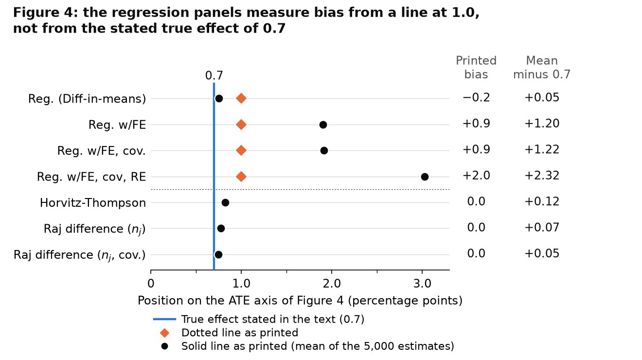
In the four regression panels of Figure 4, bias is measured from a dotted line at 1.0 percentage point and not from the stated true effect of 0.7; measured from 0.7, the biases of the fixed-effects and random-effects regressions are about 1.2 and 2.3 points instead of 0.9 and 2.0, and the figure does not establish downward bias of the difference-in-means.

Figure 4, p. 67 (PDF p. 29), the four regression panels; Section 6.5, p. 66 (PDF p. 28), first two paragraphs; Section 6.2, p. 61 (PDF p. 23), last sentence

As printed

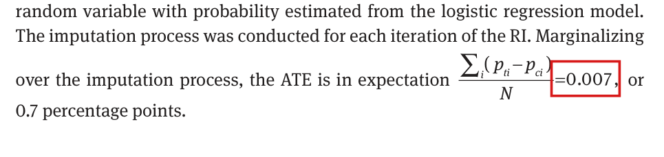
Section 6.2, p. 61, last sentence: “Marginalizing over the imputation process, the ATE is in expectation ∑i(pti−pci)N=0.007\frac{\sum_i(p_{ti}-p_{ci})}{N}=0.007, or 0.7 percentage points.”

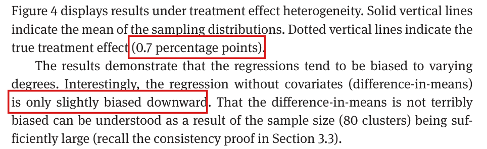
Section 6.5, p. 66, first paragraph: “Figure 4 displays results under treatment effect heterogeneity. Solid vertical lines indicate the mean of the sampling distributions. Dotted vertical lines indicate the true treatment effect (0.7 percentage points).”

Section 6.5, p. 66, second paragraph: “Interestingly, the regression without covariates (difference-in-means) is only slightly biased downward.”

Figure 4, p. 67, labels of the four regression panels, in percentage points. In each of these panels the dotted line is drawn near 1.0 on the horizontal axis.

Figure 4 as printed: labels of the regression panels.
PanelBiasSDRMSE
Reg. (Diff-in-means)−0.2\colorbox{#ffe58a}{$-0.2$}2.32.32.32.3
Reg. w/FE0.9\colorbox{#ffe58a}{$0.9$}1.51.51.8\colorbox{#ffe58a}{$1.8$}
Reg. w/FE, cov.0.9\colorbox{#ffe58a}{$0.9$}1.51.51.8\colorbox{#ffe58a}{$1.8$}
Reg. w/FE, cov, RE2.0\colorbox{#ffe58a}{$2.0$}1.31.32.4\colorbox{#ffe58a}{$2.4$}
The problem

Section 6.2 states that the true effect in the scenario with heterogeneous effects is 0.7 percentage points, and Section 6.5 says that the dotted lines of Figure 4 mark it. In the published figure, the dotted lines stand at 1.00 on the axis in the four regression panels, and each printed bias equals the position of the solid line minus the position of the dotted line, to the printed decimal. The three design-based panels show no separate dotted line. The text and the figure cannot both be right, and rounding does not reconcile them: a value printed as 0.007 lies between 0.65 and 0.75 percentage points, and every dotted line lies between 0.99 and 1.01. If the true effect is 0.7, as the text states twice, then the biases of the four regressions are about 0.3 points higher than printed: about +0.05+0.05 for the difference-in-means, +1.20+1.20 and +1.22+1.22 for the two fixed-effects regressions, and +2.32+2.32 for the random-effects regression. The RMSE labels of the fixed-effects and random-effects panels (1.81.8, 1.81.8 and 2.42.4) are then too small. From the published means and standard deviations, I obtain about 1.91.9, 1.91.9 and a value between 2.62.6 and 2.72.7. The sentence that the difference-in-means is “only slightly biased downward” rests on the printed −0.2-0.2. Measured from 0.7, the plotted mean of that estimator is higher by about 0.05, with a Monte Carlo standard error of about 0.03, so the figure does not establish downward bias.

The label “Bias = 0.0” of the Horvitz–Thompson panel also needs to be recomputed. The mean drawn in that panel is 0.82, which exceeds every target between 0.65 and 0.75 by more than 0.05. If the target is exactly 0.7, the same holds for the Des Raj panel with njn_j, whose mean is 0.77. These are disagreements between labels and plotted means in a simulation of 5,000 draws, and they do not imply that either design-based estimator is biased. The cause of the mismatch is not established, since the original simulation code and draws are not available.

Evidence a recalculation from the source

The evidence is a recalculation from the published PDF, in which Figure 4 is stored as vector artwork. The coordinates of the axis ticks, the solid lines and the dotted lines were read from the page and converted to the scale of the axis in exact rational arithmetic. The remaining ticks fit this calibration to within 0.0015 points, and the incompatibility with the stated effect persists with a tolerance of 0.005. A second, independent reading of the coordinates agrees with the first to within 0.002 points.

Figure 4, regression panels: positions of the solid line (the mean) and of the dotted line, read from the published PDF, and the bias and RMSE that follow if the true effect is 0.7. All entries are in percentage points.
PanelSolidDottedPrinted biasSolid minus 0.7Printed RMSERMSE at 0.7
Reg. (Diff-in-means)0.7530.7531.0011.001−0.2-0.2+0.053+0.0532.32.32.252.25–2.352.35
Reg. w/FE1.9041.9041.0011.0010.90.9+1.204+1.2041.81.81.881.88–1.961.96
Reg. w/FE, cov.1.9151.9150.9990.9990.90.9+1.215+1.2151.81.81.891.89–1.971.97
Reg. w/FE, cov, RE3.0243.0240.9990.9992.02.0+2.324+2.3242.42.42.642.64–2.692.69

The solid line minus the dotted line is −0.248-0.248, 0.9030.903, 0.9160.916 and 2.0252.025 in the four panels, and these values round to the printed biases. Suppose that a printed bias bb is rounded to one decimal and that the solid line is at mm. Then a target compatible with the label lies in [m−b−0.05, m−b+0.05][m-b-0.05,\,m-b+0.05]. For the four panels these intervals are [0.903,1.003][0.903,1.003], [0.954,1.054][0.954,1.054], [0.965,1.065][0.965,1.065] and [0.974,1.074][0.974,1.074], and each of them lies above 0.750.75. For the RMSE, I use the identity

E[(T−θ)2]=Var⁡(T)+(E[T]−θ)2\mathrm{E}\bigl[(T-\theta)^2\bigr]=\operatorname{Var}(T)+\bigl(\mathrm{E}[T]-\theta\bigr)^2

applied to the empirical distribution of the 5,000 estimates, with θ=0.7\theta=0.7, the plotted mean and a standard deviation within 0.050.05 of the printed one. If the standard deviation uses divisor 4,999, its square is multiplied by 4,999/5,0004{,}999/5{,}000 to give the empirical variance. The last column of the table shows the resulting approximate range. The printed 2.32.3 of the difference-in-means panel lies in its range, and the printed 1.81.8, 1.81.8 and 2.42.4 lie outside theirs. The last column gives guides rather than exact replacement labels: the plotted positions and the printed standard deviations are rounded, and the original draws are not available.

What survives

The inconsistency concerns the reporting of Figure 4 and the downward-bias sentence of Section 6.5. With the published means and standard deviations and a target near 0.7, the biases of the fixed-effects and random-effects regressions remain positive, the random-effects regression still has the smallest standard deviation, and the Horvitz–Thompson estimator remains imprecise. The grouping by RMSE is unchanged: the smallest values belong to the Des Raj estimators, and then come the fixed-effects regressions, the difference-in-means, the random-effects regression and the Horvitz–Thompson estimator. On these numbers, the statement that the Des Raj estimators are the most precise in terms of RMSE stands. The arguments on bias and consistency in Section 3 and the estimators and unbiasedness results of Sections 4 and 5 do not use Figure 4. Figures 2 and 3 come from the separate calculation under the sharp null. Figure 5 concerns standard errors and does not depend on the placement of Figure 4’s reference lines. What changes is the size of the regression biases, the RMSE labels of three panels, and the statement that the difference-in-means shows a downward bias in this example; the empirical bias labels of the design-based panels also require checking. The theoretical result that the difference-in-means can be biased is not affected.

Corrected

In Figure 4, the dotted lines should be drawn at the common, unrounded true effect of the scenario, and all empirical bias and RMSE labels should be computed from it. If that effect is 0.7 percentage points, as stated on pp. 61 and 66, then the published means and standard deviations give the following approximate labels.

Figure 4 with bias measured from 0.7: approximate labels of the regression panels, in percentage points.
PanelBiasSDRMSE
Reg. (Diff-in-means)+0.05\colorbox{#ffe58a}{$+0.05$}2.32.32.302.30
Reg. w/FE1.20\colorbox{#ffe58a}{$1.20$}1.51.51.92\colorbox{#ffe58a}{$1.92$}
Reg. w/FE, cov.1.22\colorbox{#ffe58a}{$1.22$}1.51.51.93\colorbox{#ffe58a}{$1.93$}
Reg. w/FE, cov, RE2.32\colorbox{#ffe58a}{$2.32$}1.31.32.66\colorbox{#ffe58a}{$2.66$}

Section 6.5, second paragraph: “Interestingly, the regression without covariates (difference-in-means) has a mean close to the true effect.”

Exact labels require the unrounded true effect and the original draws. Changing the text to 1.0 has not been checked against the imputation model, and it would leave the labels “Bias = 0.0” of the three design-based panels in conflict with their plotted means of 0.82, 0.77 and 0.75.
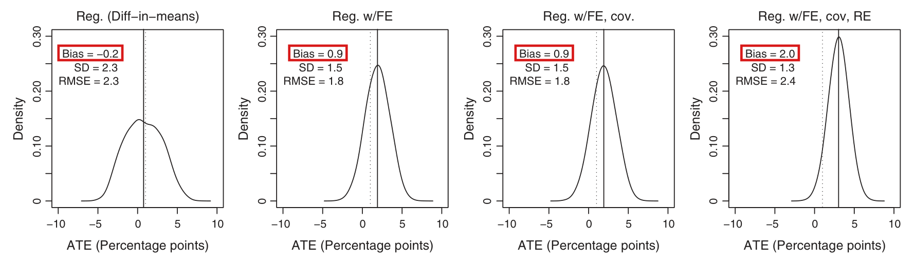
Crop of the four regression panels of Figure 4: Reg. (Diff-in-means), Reg. w/FE, Reg. w/FE, cov., and Reg. w/FE, cov, RE. Each panel shows a density curve over an axis from minus 10 to 10 percentage points, a solid vertical line at the mean and a dotted vertical line just right of zero. Red boxes mark the labels Bias = -0.2, Bias = 0.9, Bias = 0.9 and Bias = 2.0. Below them, unmarked, are SD = 2.3, 1.5, 1.5, 1.3 and RMSE = 2.3, 1.8, 1.8, 2.4.
Figure 4, p. 67 (PDF p. 29), upper row of panels, turned upright. The four marked bias labels agree, to one decimal place, with the solid line minus the dotted line, and the dotted lines stand near 1.0 on the axis, not at 0.7.
Crop of eight lines of Section 6.5. One red box marks '(0.7 percentage points)' at the end of the sentence 'Dotted vertical lines indicate the true treatment effect (0.7 percentage points).' A second red box marks 'is only slightly biased downward' in the sentence about the regression without covariates.
Section 6.5, p. 66 (PDF p. 28), first two paragraphs. The marked phrases are the true effect that the dotted lines are said to indicate and the description of the difference-in-means that rests on the printed bias of −0.2-0.2.
Chart with one row for each of the seven panels of Figure 4 and a horizontal axis from 0 to 3.3 percentage points. A blue vertical line marks 0.7, the true effect stated in the text. Orange diamonds mark the dotted lines of the four regression panels, all at 1.0. Black circles mark the solid lines: 0.75 for the difference-in-means, 1.90 and 1.92 for the two fixed-effects regressions, 3.02 for the random-effects regression, 0.82 for Horvitz-Thompson and 0.77 and 0.75 for the two Des Raj estimators. Two columns of numbers at the right give the printed bias (minus 0.2, 0.9, 0.9, 2.0, 0.0, 0.0, 0.0) and the mean minus 0.7 (0.05, 1.20, 1.22, 2.32, 0.12, 0.07, 0.05).
The lines of Figure 4 as read from the published PDF, for all seven panels. In the four regression panels the dotted line (diamond) stands at 1.0 and not at the stated true effect of 0.7 (vertical line). The columns at the right give the printed bias and the plotted mean minus 0.7, in percentage points.

Minor (8)

Real but inconsequential, for example a misprint that does not change a result.

Persistent bias does not guarantee that an estimator eventually has the larger mean squared error; the guarantee holds against a comparator whose mean squared error tends to zero.

Introduction, paragraph beginning “Bias is not the only statistical property”, p. 40 (PDF p. 2); Section 3, first paragraph, p. 42 (PDF p. 4)

See also under Formal statements (Lean): P020-T1, P020-T2

As printed

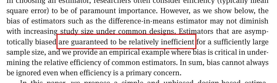
p. 40: “Estimators that are asymptotically biased are guaranteed to be relatively inefficient for a sufficiently large sample size, and we provide an empirical example where bias is critical in undermining the relative efficiency of common estimators.”

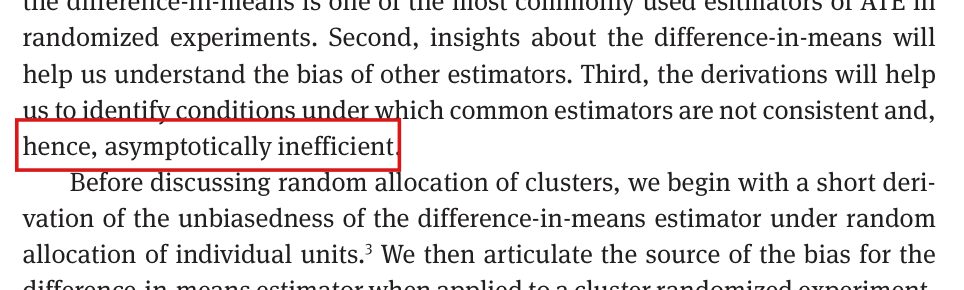
p. 42: “Third, the derivations will help us to identify conditions under which common estimators are not consistent and, hence, asymptotically inefficient.”

The problem

The paragraph on p. 40 measures efficiency by mean squared error. The marked sentence says that an estimator whose bias does not vanish must, in a large enough sample, have a larger mean squared error than the estimator with which it is compared, and the sentence on p. 42 draws the same conclusion from inconsistency. One sufficient condition is that the mean squared error of that comparator tend to zero, which neither sentence assumes. If asymptotic efficiency is defined so as to require consistency, the phrase on p. 42 holds by definition, but that reading gives no ranking by mean squared error and does not support the sentence on p. 40. The asymptotic regimes of the paper include the one in which the number of clusters is fixed and the clusters grow (p. 40 and Section 3.3, p. 47). In that regime the variance of an unbiased estimator need not vanish, and a biased estimator can keep the smaller mean squared error at every sample size.

Evidence an exact counterexample

The evidence is an exact counterexample, computed by enumerating every assignment in rational arithmetic. Let M=3M=3, mt=1m_t=1 and mc=2m_c=2, and let the clusters have sizes 11, 22 and 44. The control outcomes of the individuals are (0)(0), (1,0)(1,0) and (1,0,0,0)(1,0,0,0) in the three clusters, and every treatment outcome is 00. Then N=7N=7 and Δ=−2/7\Delta=-2/7. Each cluster is the treated one with probability 1/31/3. Enumerating the three assignments, I obtain the following values of the estimators.

The three-cluster example: the estimate under each of the three equally likely assignments, and the bias and mean squared error of each estimator. The average treatment effect is −2/7-2/7.
Treated clusterDifference in meansHorvitz–ThompsonDes Raj, k=2/21k=2/21
1−1/3-1/3−3/7-3/7−17/49-17/49
2−1/5-1/5−3/14-3/14−19/98-19/98
3−1/3-1/3−3/14-3/14−31/98-31/98
Bias−1/315-1/3150000
Mean squared error131/33075≈0.00396131/33075\approx0.003961/98≈0.010201/98\approx0.010203/686≈0.004373/686\approx0.00437

For a fixed kk the Des Raj estimator of Section 5.1 is unbiased, and I find that its mean squared error is 3/686+(9/14)(k−2/21)23/686+(9/14)(k-2/21)^2. This implies that no fixed kk does better than 3/6863/686. The choice k=0k=0 is the Horvitz–Thompson estimator. Now suppose that each individual is copied hh times within its cluster, as in the construction on p. 47. The cluster sizes and totals are multiplied by hh, and N=7hN=7h. Every entry of the table is then the same for every hh. I conclude that the difference in means has bias −1/315-1/315 at every sample size. It is inconsistent, since its error is at least 1/211/21 in absolute value under every assignment. Its mean squared error is nevertheless smaller than that of the Horvitz–Thompson estimator and of the Des Raj estimator with any fixed kk.

The corrected statement holds because mean squared error is the sum of the variance and the squared bias. Suppose that the bias bhb_h of ThT_h tends to b≠0b\neq0. Then MSE⁡(Th)≥bh2>b2/4\operatorname{MSE}(T_h)\ge b_h^2>b^2/4 for all large hh. If also MSE⁡(Uh)→0\operatorname{MSE}(U_h)\to0, then MSE⁡(Uh)<b2/4\operatorname{MSE}(U_h)<b^2/4 for all large hh.

What survives

I found no use of the guarantee in the derivations checked. The bias formula and the replication arguments of Section 3 are unaffected, and so are the results on the Horvitz–Thompson estimator in Section 4. The same holds for the results of Section 5 on the Des Raj estimator: that it is unbiased, and the explicit comparison of its variance with that of the Horvitz–Thompson estimator. The rankings by root mean squared error in Sections 6.4 and 6.5 are computed for the application and do not rest on these sentences. The motivation survives in the weaker form of the next sentence of the paper: bias cannot always be ignored when efficiency is the concern. The counterexample does not show that biased estimators are better in general.

Corrected

p. 40: “Persistent asymptotic bias contributes a nonvanishing squared-bias term to mean squared error and can undermine relative efficiency. It guarantees eventual mean-squared-error inferiority to a specified comparator when that comparator’s mean squared error tends to zero.” The clause on the empirical example is unchanged.

p. 42: “… conditions under which common estimators are not consistent; whether they are relatively inefficient depends on comparative mean squared errors.”

In full: let ThT_h and UhU_h be estimators of Δh\Delta_h along a sequence of finite populations indexed by hh, each with finite second moment, such that the bias of ThT_h converges to a limit b≠0b\neq0 and MSE⁡(Uh)→0\operatorname{MSE}(U_h)\to0 as h→∞h\to\infty. Then MSE⁡(Uh)<MSE⁡(Th)\operatorname{MSE}(U_h)<\operatorname{MSE}(T_h) for all sufficiently large hh.

Crop of the Introduction paragraph on efficiency. A red box marks the words 'are guaranteed to be relatively inefficient' in the sentence 'Estimators that are asymptotically biased are guaranteed to be relatively inefficient for a sufficiently large sample size'. The lines above read 'researchers often consider efficiency (typically mean square error) to be of paramount importance'.
Introduction, p. 40 (PDF p. 2). The marked words state the guarantee; two sentences earlier the paragraph takes efficiency to be “typically mean square error”.
Crop of the first paragraph of Section 3. A red box marks the words 'hence, asymptotically inefficient' at the end of the sentence 'Third, the derivations will help us to identify conditions under which common estimators are not consistent and, hence, asymptotically inefficient.'
Section 3, first paragraph, p. 42 (PDF p. 4). The marked words draw the same inference from inconsistency.

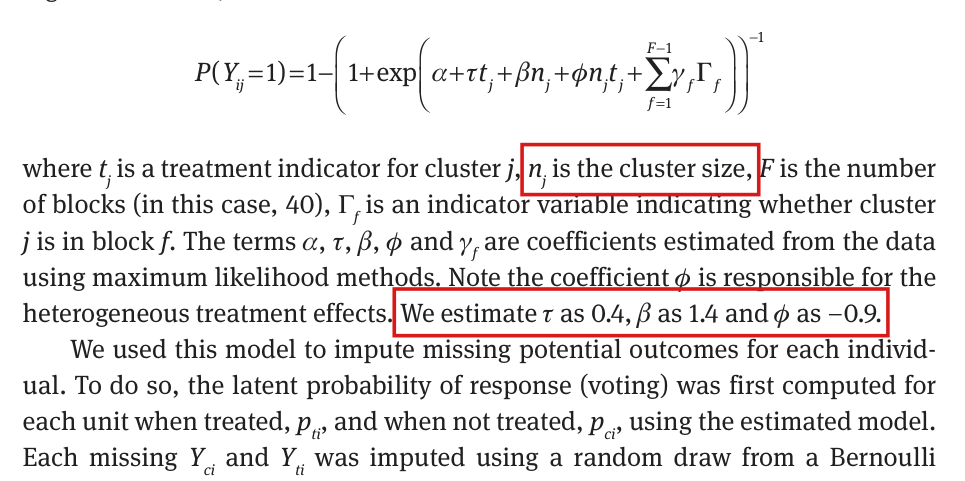
With njn_j the number of individuals in a cluster, the printed coefficients τ=0.4\tau=0.4 and ϕ=−0.9\phi=-0.9 make the modelled effect negative for every individual, against the reported average effect of +0.007+0.007; the predictor’s units and coefficients should be reconciled.

Section 6.2, p. 61 (PDF p. 23): the logistic regression model, the sentence that reports the coefficients, and the last sentence of the section

See also under Formal statements (Lean): P020-T3, P020-T4

As printed
P(Yij=1)=1−(1+exp⁡(α+τtj+βnj+ϕnjtj+∑f=1F−1γfΓf))−1P(Y_{ij}=1)=1-\left(1+\exp\left(\alpha+\tau t_j+\beta \colorbox{#ffe58a}{$\displaystyle n_j$}+\phi \colorbox{#ffe58a}{$\displaystyle n_j$}t_j+\sum_{f=1}^{F-1}\gamma_f\Gamma_f\right)\right)^{-1}

“where tjt_j is a treatment indicator for cluster jj, nj\colorbox{#ffe58a}{$n_j$} is the cluster size, FF is the number of blocks (in this case, 40), Γf\Gamma_f is an indicator variable indicating whether cluster jj is in block ff. The terms α\alpha, τ\tau, β\beta, ϕ\phi and γf\gamma_f are coefficients estimated from the data using maximum likelihood methods. Note the coefficient ϕ\phi is responsible for the heterogeneous treatment effects. We estimate τ\tau as 0.4, β\beta as 1.4 and ϕ\phi as −0.9\colorbox{#ffe58a}{$-0.9$}.”

“Marginalizing over the imputation process, the ATE is in expectation

∑i(pti−pci)N=0.007,\frac{\sum_i(p_{ti}-p_{ci})}{N}\colorbox{#ffe58a}{$\displaystyle =0.007$},

or 0.7 percentage points.”

The problem

The paper defines njn_j as the number of individuals in cluster jj (p. 44), and Section 6.2 does not rescale it. For an individual in cluster jj, the difference between the linear predictors under treatment and under control is τ+ϕnj=0.4−0.9 nj\tau+\phi n_j=0.4-0.9\,n_j, which is at most −0.5-0.5 when nj≥1n_j\ge1. Since the printed probability is an increasing function of the linear predictor, I have pti<pcip_{ti}<p_{ci} for every individual. The average of pti−pcip_{ti}-p_{ci} is then negative for all values of α\alpha, β\beta and γf\gamma_f, and it cannot equal 0.0070.007. In the public file of the source study the clusters hold between 30 and 990 voters. A plausible explanation is that cluster size entered the fit in other units, such as thousands of voters, but the paper does not say so, and the scale cannot be recovered from the text.

Evidence a historical Lean attribution (Generated status: clause support not certified in this release)

The evidence is the derivation above, together with a Lean 4 proof of the same statement for the model as printed, which covers every finite nonempty population. Rounding does not change the sign: coefficients that round to 0.40.4 and −0.9-0.9 are at most 0.450.45 and −0.85-0.85, so that τ+ϕnj≤−0.40\tau+\phi n_j\le-0.40 when nj≥1n_j\ge1. As a check of the scale only, I fitted the same model to all 85 clusters of the public file with cluster size in thousands. The fit gives τ=0.43\tau=0.43, β=1.43\beta=1.43 and ϕ=−0.99\phi=-0.99, with an average of pti−pcip_{ti}-p_{ci} equal to 0.0100.010. This is not the fit to 80 clusters that the paper reports, and it does not reproduce 0.0070.007.

What survives

The results on the estimators and their variances in Sections 2–5 and the appendices do not use the fitted coefficients. The scenario under the sharp null in Section 6.4 and Figures 2 and 3 uses a separate imputation and is unaffected. Section 6.5 and Figures 4 and 5 use the scenario with heterogeneous effects. No result there is shown to change, but the scenario cannot be reproduced from the model as printed. The units that were used and the coefficients of the fit to 80 clusters are not recovered.

Corrected

The passage should state the units of the cluster-size predictor and give the coefficients in those units. If the predictor was cluster size in thousands of individuals, the passage reads:

P(Yij=1)=1−(1+exp⁡(α+τtj+βsj+ϕsjtj+∑f=1F−1γfΓf))−1P(Y_{ij}=1)=1-\left(1+\exp\left(\alpha+\tau t_j+\beta \colorbox{#ffe58a}{$\displaystyle s_j$}+\phi \colorbox{#ffe58a}{$\displaystyle s_j$}t_j+\sum_{f=1}^{F-1}\gamma_f\Gamma_f\right)\right)^{-1}

“where tjt_j is a treatment indicator for cluster jj, sj=nj/1000\colorbox{#ffe58a}{$s_j=n_j/1000$} is the cluster size in thousands of individuals, FF is the number of blocks (in this case, 40), Γf\Gamma_f is an indicator variable indicating whether cluster jj is in block ff.” The coefficients are then as printed: τ=0.4\tau=0.4, β=1.4\beta=1.4 and ϕ=−0.9\phi=-0.9.

Equivalently, the passage can keep njn_j and report β\beta as 0.00140.0014 and ϕ\phi as −0.0009-0.0009. With this scale the difference 0.4−0.0009 nj0.4-0.0009\,n_j is positive for clusters of fewer than 4000/9≈444.44000/9\approx444.4 individuals and negative for larger ones, and the contradiction in sign disappears. The scale in thousands is an inference; the specification that was used has not been recovered. The reported value 0.0070.007 should be checked on the sample of 80 clusters.

Crop of the logistic regression model P(Y_ij = 1) = 1 - (1 + exp(alpha + tau t_j + beta n_j + phi n_j t_j + sum of gamma_f Gamma_f)) to the power -1 and of the paragraph below it. Red boxes mark 'n_j is the cluster size,' and the sentence 'We estimate tau as 0.4, beta as 1.4 and phi as -0.9.'
The logistic model of Section 6.2, p. 61 (PDF p. 23). The marked passages define njn_j as the cluster size and report the coefficients; with njn_j a count of individuals, 0.4−0.9 nj0.4-0.9\,n_j is negative for every cluster.
Crop of the last three lines of Section 6.2. A red box marks '= 0.007,' in 'Marginalizing over the imputation process, the ATE is in expectation the sum over i of (p_ti - p_ci) divided by N = 0.007, or 0.7 percentage points.'
Last sentence of Section 6.2, p. 61 (PDF p. 23). The marked value is the positive average effect that the model is reported to give.

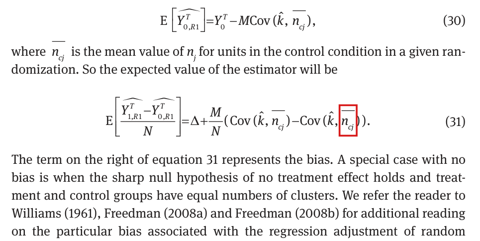
In equation (31) the second covariance is with the mean cluster size in the treatment arm, ntj‾\overline{n_{tj}}, as in the same formula in Section 5.3 (p. 57).

Appendix B, equation (31), p. 71 (PDF p. 33)

See also under Formal statements (Lean): P020-T5, P020-T6

As printed
E[Y1,R1T^−Y0,R1T^N]=Δ+MN(Cov⁡(k^,ncj‾)−Cov⁡(k^,ncj‾)).(31)\mathrm{E}\left[\frac{\widehat{Y^T_{1,R1}}-\widehat{Y^T_{0,R1}}}{N}\right]=\Delta+\frac{M}{N}\left(\operatorname{Cov}(\hat k,\overline{n_{cj}})-\operatorname{Cov}(\hat k,\overline{n_{\colorbox{#ffe58a}{$\displaystyle c$}j}})\right).\qquad(31)
The problem

As printed, the two covariances in (31) are the same, and the term that the next sentence calls the bias is identically zero. Subtracting equation (30) from equation (29), I obtain the treatment-arm mean ntj‾\overline{n_{tj}} in the second covariance, and Section 5.3 prints the formula in that form on p. 57. The second subscript cc is a misprint.

Evidence a derivation

The evidence is a derivation and an exact example. Let ntj‾\overline{n_{tj}} and ncj‾\overline{n_{cj}} be the mean sizes of the clusters assigned to treatment and to control in a given randomization, so that E[ntj‾]=E[ncj‾]=N/M\mathrm{E}[\overline{n_{tj}}]=\mathrm{E}[\overline{n_{cj}}]=N/M. The estimator k^\hat k is constant within a randomization. By equation (21) with k^\hat k in place of kk, I have

Y1,R1T^=Mmt∑j∈J1YjT−Mk^(ntj‾−NM).\widehat{Y^T_{1,R1}}=\frac{M}{m_t}\sum_{j\in J_1}Y_j^T-M\hat k\Bigl(\overline{n_{tj}}-\frac{N}{M}\Bigr).

Taking expectations, I obtain

E[Y1,R1T^]=Y1T−M(E[k^ ntj‾]−E[k^] E[ntj‾])=Y1T−MCov⁡(k^,ntj‾),\mathrm{E}\bigl[\widehat{Y^T_{1,R1}}\bigr]=Y_1^T-M\bigl(\mathrm{E}[\hat k\,\overline{n_{tj}}]-\mathrm{E}[\hat k]\,\mathrm{E}[\overline{n_{tj}}]\bigr)=Y_1^T-M\operatorname{Cov}(\hat k,\overline{n_{tj}}),

which is equation (29). By the same argument for the control arm, I have equation (30), E[Y0,R1T^]=Y0T−MCov⁡(k^,ncj‾)\mathrm{E}\bigl[\widehat{Y^T_{0,R1}}\bigr]=Y_0^T-M\operatorname{Cov}(\hat k,\overline{n_{cj}}). Subtracting (30) from (29) and dividing by NN, I obtain the corrected (31), since Δ=(Y1T−Y0T)/N\Delta=(Y_1^T-Y_0^T)/N.

For the example, take M=3M=3 clusters of sizes (1,2,3)(1,2,3), so that N=6N=6, with one cluster treated. Let the cluster totals be (0,0,0)(0,0,0) under control and (0,0,3)(0,0,3) under treatment, so that Δ=1/2\Delta=1/2, and let k^\hat k be the least-squares slope of the observed cluster totals on njn_j, with an intercept. Over the three assignments, k^\hat k takes the values (0,0,3/2)(0,0,3/2) and the estimator takes the values (0,0,3/8)(0,0,3/8). Its expectation is 1/81/8, and its bias is −3/8-3/8. Here Cov⁡(k^,ncj‾)=−1/4\operatorname{Cov}(\hat k,\overline{n_{cj}})=-1/4 and Cov⁡(k^,ntj‾)=1/2\operatorname{Cov}(\hat k,\overline{n_{tj}})=1/2, and the bias term of the corrected formula is (3/6)(−1/4−1/2)=−3/8(3/6)(-1/4-1/2)=-3/8. The printed formula gives 00.

What survives

Equations (29) and (30), their derivation and the bias formula of Section 5.3 are correct as printed. The unbiasedness of the Des Raj estimator for a coefficient kk fixed before the analysis is not affected. Only the last display of Appendix B changes.

Corrected

Let MM clusters of sizes njn_j, with N=∑jnjN=\sum_j n_j, be completely randomized, mtm_t to treatment and mc=M−mtm_c=M-m_t to control. Let k^\hat k be an estimator of kk computed from the data of the same experiment, so that it is constant within a randomization and can vary across randomizations. Let ntj‾\overline{n_{tj}} and ncj‾\overline{n_{cj}} be the mean sizes of the clusters in treatment and in control in a given randomization. Then the Des Raj difference estimator of equations (20) and (21), with k^\hat k in place of kk, satisfies

E[Y1,R1T^−Y0,R1T^N]=Δ+MN(Cov⁡(k^,ncj‾)−Cov⁡(k^,ntj‾)).(31)\mathrm{E}\left[\frac{\widehat{Y^T_{1,R1}}-\widehat{Y^T_{0,R1}}}{N}\right]=\Delta+\frac{M}{N}\left(\operatorname{Cov}(\hat k,\overline{n_{cj}})-\operatorname{Cov}(\hat k,\overline{n_{\colorbox{#ffe58a}{$\displaystyle t$}j}})\right).\qquad(31)
Crop of the end of Appendix B: equation (30), the sentence 'So the expected value of the estimator will be', equation (31) and the paragraph that follows. A red box marks the second argument of the second covariance in equation (31), n bar with subscript c j. The first covariance in the same equation has the same argument, unmarked.
Appendix B, p. 71 (PDF p. 33), equations (30) and (31). The marked term in (31) repeats the control-arm mean ncj‾\overline{n_{cj}} of the first covariance.

Local misprints in labels, indices, cross-references and one bracket: among them, the control sum in the second line of equation (25) should contain U0jTU^T_{0j}, and the expectation in the second line of the display that ends in equation (35) should enclose both factors.

Section 3.3, p. 47 (PDF p. 9); p. 51 (PDF p. 13); p. 54 (PDF p. 16); p. 55 (PDF p. 17); equation (25), p. 56 (PDF p. 18); p. 58 (PDF p. 20); Appendix B, p. 71 (PDF p. 33); Appendix C, p. 72 (PDF p. 34)

See also under Formal statements (Lean): P020-T7, P020-T8, P020-T9, P020-T15

As printed
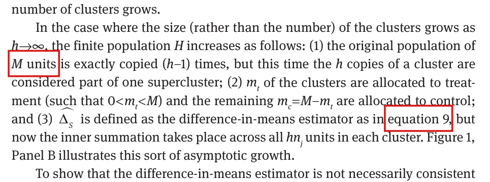
  1. p. 47: “(1) the original population of MM units is exactly copied (h−1)(h-1) times, but this time the hh copies of a cluster are considered part of one supercluster”
  2. p. 47: “(3) ΔS^\widehat{\Delta_S} is defined as the difference-in-means estimator as in equation 9, but now the inner summation takes place across all hnjhn_j units in each cluster”
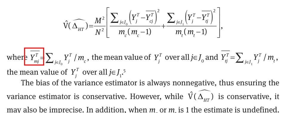
  3. p. 51: “where YmjT‾=∑j∈J0YjT/mc\colorbox{#ffe58a}{$\overline{Y^T_{mj}}$}=\sum_{j\in J_0}Y^T_j/m_c, the mean value of YjTY^T_j over all j∈J0j\in J_0”
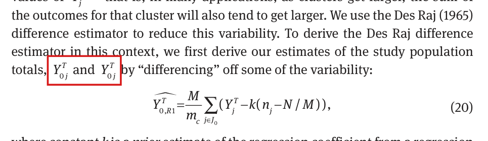
  4. p. 54: “we first derive our estimates of the study population totals, Y0jT\colorbox{#ffe58a}{$Y^T_{0j}$} and Y0jT\colorbox{#ffe58a}{$Y^T_{0j}$}”
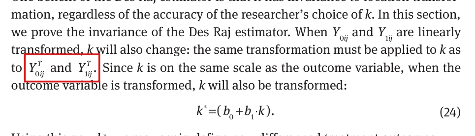
  5. p. 55: “the same transformation must be applied to kk as to Y0ijT\colorbox{#ffe58a}{$Y^T_{0ij}$} and Y1ijT\colorbox{#ffe58a}{$Y^T_{1ij}$}”
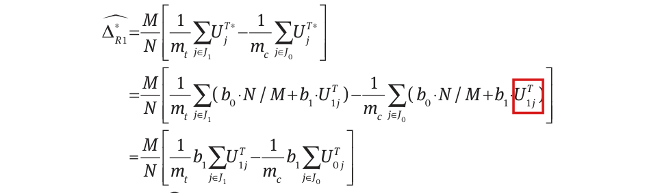
  6. p. 56, equation (25), second line:
    =MN[1mt∑j∈J1(b0⋅N/M+b1⋅U1jT)−1mc∑j∈J0(b0⋅N/M+b1⋅U1jT)]=\frac{M}{N}\left[\frac{1}{m_t}\sum_{j\in J_1}(b_0\cdot N/M+b_1\cdot U^T_{1j})-\frac{1}{m_c}\sum_{j\in J_0}(b_0\cdot N/M+b_1\cdot \colorbox{#ffe58a}{$\displaystyle U^T_{1j}$})\right]
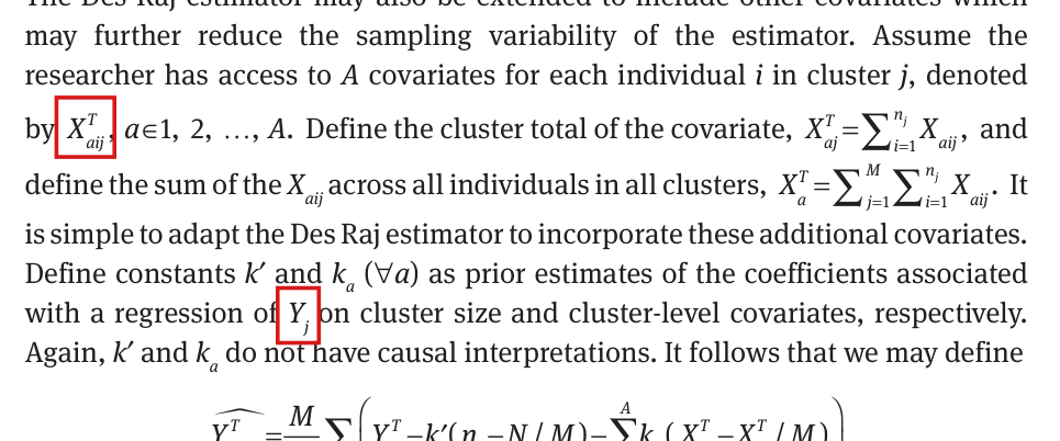
  7. p. 58: “AA covariates for each individual ii in cluster jj, denoted by XaijT\colorbox{#ffe58a}{$X^T_{aij}$}”
  8. p. 58: “with a regression of Yj\colorbox{#ffe58a}{$Y_j$} on cluster size and cluster-level covariates”
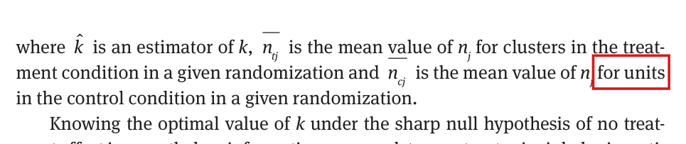
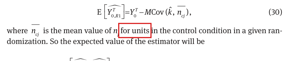
  9. pp. 58 and 71: “ncj‾\overline{n_{cj}} is the mean value of njn_j for units in the control condition in a given randomization”
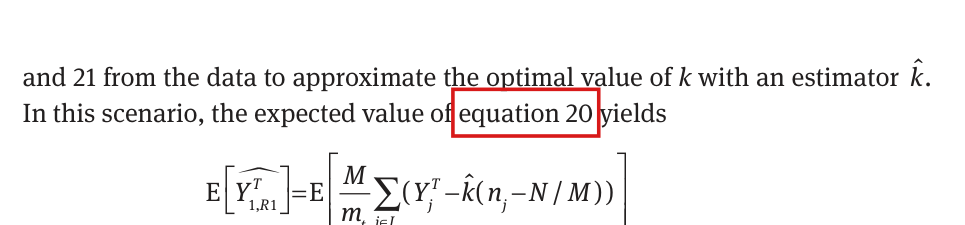
  10. p. 71: “In this scenario, the expected value of equation 20 yields”, followed by the expectation of Y1,R1T^\widehat{Y^T_{1,R1}}
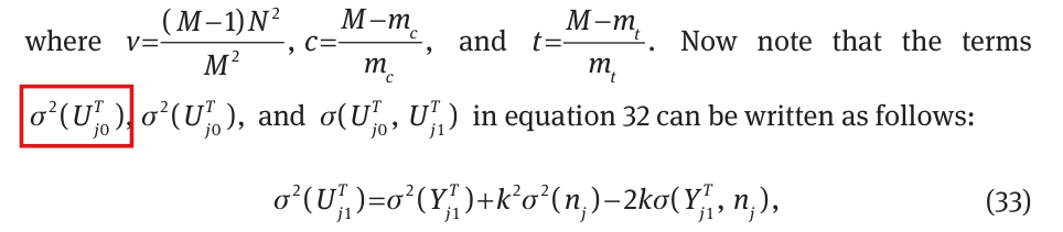
  11. p. 72: “Now note that the terms σ2(Uj0T)\colorbox{#ffe58a}{$\sigma^2(U^T_{j0})$}, σ2(Uj0T)\sigma^2(U^T_{j0}), and σ(Uj0T,Uj1T)\sigma(U^T_{j0},U^T_{j1}) in equation 32 can be written as follows”
  12. p. 72, second line of the display that ends in equation (35):
    =E[Yj0T−kδj](Yj1T−kδj)−Y0T‾ Y1T‾=\mathrm{E}[Y^T_{j0}-k\delta_j\colorbox{#ffe58a}{$\displaystyle ]$}(Y^T_{j1}-k\delta_j)-\overline{Y^T_0}\,\overline{Y^T_1}
The problem

Each item is a slip in a label, an index, a cross-reference or a bracket, and the neighbouring lines show the intended form. In items 6 and 12 a displayed line is false as printed.

  1. MM is the number of clusters (p. 44), and the parallel construction on p. 46 says “MM clusters”.
  2. Equation 9 is a probability limit. The estimator with an inner summation is defined in equation 6.
  3. The display above the clause writes the control mean as YcjT‾\overline{Y^T_{cj}}.
  4. Equations (20) and (21) estimate the population totals Y0TY^T_0 and Y1TY^T_1. The symbol Y0jTY^T_{0j} is the control total of cluster jj (p. 48).
  5. The superscript TT marks a total (p. 48). Individual outcomes do not carry it.
  6. The sentence before the display defines U0jT∗=b0⋅N/M+b1⋅U0jTU^{T*}_{0j}=b_0\cdot N/M+b_1\cdot U^T_{0j} for the control clusters, and the third line of the display has U0jTU^T_{0j} in the sum over J0J_0.
  7. The individual covariate is XaijX_{aij}. The same paragraph defines the total XajT=∑i=1njXaijX^T_{aj}=\sum_{i=1}^{n_j}X_{aij}.
  8. The regression is of the cluster total YjTY^T_j, as on p. 54.
  9. The mean ncj‾\overline{n_{cj}} is taken over the clusters in the control condition. The clause for ntj‾\overline{n_{tj}} says “for clusters in the treatment condition”.
  10. Equation 20 defines the estimator of the control total. The display that follows is the expectation of the estimator of the treatment total, equation 21.
  11. Equation 32 has one variance for each arm, and the expansions that follow, “respectively”, are (33) for σ2(Uj1T)\sigma^2(U^T_{j1}), (34) for σ2(Uj0T)\sigma^2(U^T_{j0}) and (35) for the covariance.
  12. The expectation is of the product of the two factors. The next line of the display expands that product inside the expectation.

Note that Appendix C writes the indices in the order j0j0, j1j1, and the main text writes 0j0j, 1j1j. This is a relabelling and needs no correction.

Evidence a derivation

The evidence is a check of the pages against the definitions on pp. 44, 46, 48 and 54, with a derivation for the two displayed lines. In equation (25), with U0jTU^T_{0j} in the control sum, the constants b0⋅N/Mb_0\cdot N/M cancel between the two arm means, and b1b_1 times the original estimator remains. For example, let the cluster sizes be (1,2)(1,2), the control totals (0,0)(0,0) and the treatment totals (1,2)(1,2), with k=0k=0, b0=0b_0=0 and b1=1b_1=1, and let the first cluster be treated. Then the estimate is 2/32/3, and the second line as printed evaluates to −2/3-2/3. In the display that ends in equation (35), E\mathrm{E} is the average over the MM clusters and δj=nj−N/M\delta_j=n_j-N/M has average zero. Expanding E[(Yj0T−kδj)(Yj1T−kδj)]−Y0T‾ Y1T‾\mathrm{E}[(Y^T_{j0}-k\delta_j)(Y^T_{j1}-k\delta_j)]-\overline{Y^T_0}\,\overline{Y^T_1}, I obtain σ(Yj0T,Yj1T)−kσ(Yj0T,nj)−kσ(Yj1T,nj)+k2σ2(nj)\sigma(Y^T_{j0},Y^T_{j1})-k\sigma(Y^T_{j0},n_j)-k\sigma(Y^T_{j1},n_j)+k^2\sigma^2(n_j), which is equation (35). With k=0k=0 and both vectors of totals equal to (0,2)(0,2), the covariance is 11. The line as printed instead equals E[Yj0T] Yj1T−1=Yj1T−1\mathrm{E}[Y^T_{j0}]\,Y^T_{j1}-1=Y^T_{j1}-1, which is −1-1 for one cluster and 11 for the other.

What survives

No result changes. Equation (10), the variance estimator on p. 51, the estimators (20) and (21), the invariance result (25), the bias formulas (29) and (30) and the optimal kk of Appendix C hold once the slips are corrected. The last lines of the displays (25) and (35) are correct as printed.

Corrected
  1. p. 47: “(1) the original population of MM clusters is exactly copied (h−1)(h-1) times”
  2. p. 47: “(3) ΔS^\widehat{\Delta_S} is defined as the difference-in-means estimator as in equation 6”
  3. p. 51: “where YcjT‾=∑j∈J0YjT/mc\colorbox{#ffe58a}{$\overline{Y^T_{cj}}$}=\sum_{j\in J_0}Y^T_j/m_c”
  4. p. 54: “the study population totals, Y0T\colorbox{#ffe58a}{$Y^T_0$} and Y1T\colorbox{#ffe58a}{$Y^T_1$}”
  5. p. 55: “the same transformation must be applied to kk as to Y0ij\colorbox{#ffe58a}{$Y_{0ij}$} and Y1ij\colorbox{#ffe58a}{$Y_{1ij}$}”
  6. p. 56, equation (25):
    ΔR1∗^=MN[1mt∑j∈J1UjT∗−1mc∑j∈J0UjT∗]=MN[1mt∑j∈J1(b0⋅N/M+b1⋅U1jT)−1mc∑j∈J0(b0⋅N/M+b1⋅U0jT)]=MN[1mtb1∑j∈J1U1jT−1mcb1∑j∈J0U0jT]=b1⋅ΔR1^.\begin{aligned} \widehat{\Delta^*_{R1}}&=\frac{M}{N}\left[\frac{1}{m_t}\sum_{j\in J_1}U^{T*}_j-\frac{1}{m_c}\sum_{j\in J_0}U^{T*}_j\right]\\ &=\frac{M}{N}\left[\frac{1}{m_t}\sum_{j\in J_1}(b_0\cdot N/M+b_1\cdot U^T_{1j})-\frac{1}{m_c}\sum_{j\in J_0}(b_0\cdot N/M+b_1\cdot \colorbox{#ffe58a}{$\displaystyle U^T_{0j}$})\right]\\ &=\frac{M}{N}\left[\frac{1}{m_t}b_1\sum_{j\in J_1}U^T_{1j}-\frac{1}{m_c}b_1\sum_{j\in J_0}U^T_{0j}\right]\\ &=b_1\cdot\widehat{\Delta_{R1}}. \end{aligned}
  7. p. 58: “denoted by Xaij\colorbox{#ffe58a}{$X_{aij}$}”
  8. p. 58: “with a regression of YjT\colorbox{#ffe58a}{$Y^T_j$} on cluster size and cluster-level covariates”
  9. pp. 58 and 71: “ncj‾\overline{n_{cj}} is the mean value of njn_j for clusters in the control condition in a given randomization”
  10. p. 71: “In this scenario, the expected value of equation 21 yields”
  11. p. 72: “Now note that the terms σ2(Uj1T)\colorbox{#ffe58a}{$\sigma^2(U^T_{j1})$}, σ2(Uj0T)\sigma^2(U^T_{j0}), and σ(Uj0T,Uj1T)\sigma(U^T_{j0},U^T_{j1}) in equation 32 can be written as follows”
  12. p. 72, with δj=nj−N/M\delta_j=n_j-N/M and E\mathrm{E} the average over the MM clusters:
    σ(Uj0T,Uj1T)=E[Uj0TUj1T]−U0T‾ U1T‾=E[(Yj0T−kδj)(Yj1T−kδj)]−Y0T‾ Y1T‾=σ(Yj0T,Yj1T)−kσ(Yj0T,nj)−kσ(Yj1T,nj)+k2σ2(nj).\begin{aligned} \sigma(U^T_{j0},U^T_{j1})&=\mathrm{E}[U^T_{j0}U^T_{j1}]-\overline{U^T_0}\,\overline{U^T_1}\\ &=\mathrm{E}[\colorbox{#ffe58a}{$\displaystyle ($}Y^T_{j0}-k\delta_j\colorbox{#ffe58a}{$\displaystyle )$}(Y^T_{j1}-k\delta_j)\colorbox{#ffe58a}{$\displaystyle ]$}-\overline{Y^T_0}\,\overline{Y^T_1}\\ &=\sigma(Y^T_{j0},Y^T_{j1})-k\sigma(Y^T_{j0},n_j)-k\sigma(Y^T_{j1},n_j)+k^2\sigma^2(n_j). \end{aligned}
Crop of the paragraph that sets up growth in cluster size. Red boxes mark 'M units' in 'the original population of M units is exactly copied (h-1) times' and 'equation 9' in 'is defined as the difference-in-means estimator as in equation 9, but now the inner summation takes place across all h n_j units in each cluster'.
Section 3.3, p. 47 (PDF p. 9), items 1 and 2. The marked words call the MM clusters “units” and cite equation 9, a probability limit, for the definition of the estimator.
Crop of the display for the variance estimator V-hat of Delta-hat-HT, whose first sum contains Y_j^T minus Y-bar_cj^T, and of the sentence below it. A red box marks the symbol Y-bar_mj^T in 'where Y-bar_mj^T equals the sum over j in J_0 of Y_j^T divided by m_c'.
The variance estimator and its “where” clause, p. 51 (PDF p. 13), item 3. The display uses the control mean with subscript cjcj; the marked symbol in the definition has subscript mjmj.
Crop of the lines that introduce equation (20). A red box marks 'Y_0j^T and Y_0j^T' in 'we first derive our estimates of the study population totals, Y_0j^T and Y_0j^T by differencing off some of the variability'. Equation (20) follows.
Sentence before equation (20), p. 54 (PDF p. 16), item 4. The marked symbols name the control total of cluster jj twice where the two population totals are meant.
Crop of the first paragraph of Section 5.2 and equation (24). A red box marks 'Y_0ij^T and Y_1ij^T' in 'the same transformation must be applied to k as to Y_0ij^T and Y_1ij^T'. Two lines above, the text reads 'When Y_0ij and Y_1ij are linearly transformed'.
Section 5.2, first paragraph, p. 55 (PDF p. 17), item 5. The marked individual outcomes carry the superscript TT of a total; the same outcomes are printed without it two lines above.
Crop of the first three lines of equation (25). In the second line a red box marks U_1j^T inside the sum over j in J_0 of (b_0 N/M + b_1 U_1j^T). The third line reads M over N times the bracket of one over m_t times b_1 times the sum over J_1 of U_1j^T minus one over m_c times b_1 times the sum over J_0 of U_0j^T.
Equation (25), first three lines, p. 56 (PDF p. 18), item 6. In the second line the marked term in the sum over the control clusters J0J_0 is U1jTU^T_{1j}; the third line has U0jTU^T_{0j} in the same sum.
Crop of the first lines of the page. A red box marks 'for units' in 'n-bar_cj is the mean value of n_j for units in the control condition in a given randomization'. The line above reads 'n-bar_tj is the mean value of n_j for clusters in the treatment condition'.
First lines of p. 58 (PDF p. 20), item 9. The marked words take the mean of njn_j over “units” in the control condition; the parallel clause for the treatment condition says “clusters”.
Crop of the first paragraph of Section 5.4. Red boxes mark X_aij^T in 'A covariates for each individual i in cluster j, denoted by X_aij^T' and Y_j in 'a regression of Y_j on cluster size and cluster-level covariates'. The same paragraph defines the cluster total X_aj^T as the sum over i of X_aij.
Section 5.4, first paragraph, p. 58 (PDF p. 20), items 7 and 8. The marked individual covariate carries the superscript TT, and the marked outcome of the regression lacks it.
Crop of the top of the page. A red box marks 'equation 20' in 'In this scenario, the expected value of equation 20 yields'. The display below begins with the expectation of Y-hat_1,R1^T, written with M over m_t and a sum over j in J_1.
Appendix B, sentence before equation (29), p. 71 (PDF p. 33), item 10. The marked reference is to equation 20, the estimator of the control total; the display that follows is the expectation of the estimator of the treatment total, equation 21.
Crop of equation (30) and the sentence after it. A red box marks 'for units' in 'where n-bar_cj is the mean value of n_j for units in the control condition in a given randomization'.
Appendix B, sentence after equation (30), p. 71 (PDF p. 33), item 9. The marked words repeat “for units” from p. 58.
Crop of the top of the page and equation (33). A red box marks the first of two identical terms sigma squared of U_j0^T in 'Now note that the terms sigma squared of U_j0^T, sigma squared of U_j0^T, and sigma of U_j0^T, U_j1^T in equation 32 can be written as follows'. Equation (33) below expands sigma squared of U_j1^T.
Appendix C, sentence before equation (33), p. 72 (PDF p. 34), item 11. The list names σ2(Uj0T)\sigma^2(U^T_{j0}) twice; the first, marked, should be σ2(Uj1T)\sigma^2(U^T_{j1}), the term expanded in equation (33).
Crop of three lines of a display. The first line reads sigma of U_j0^T, U_j1^T equals E[U_j0^T U_j1^T] minus U-bar_0^T U-bar_1^T. In the second line a red box marks 'E[Y_j0^T - k delta_j](Y_j1^T - k delta_j)', where the square bracket closes after the first factor. The third line reads E[Y_j0^T Y_j1^T - Y_j0^T k delta_j - Y_j1^T k delta_j + k squared delta_j squared] minus Y-bar_0^T Y-bar_1^T.
Appendix C, first three lines of the display that ends in equation (35), p. 72 (PDF p. 34), item 12. In the marked expression the bracket of the expectation closes before the second factor; the next line expands the product inside the expectation.

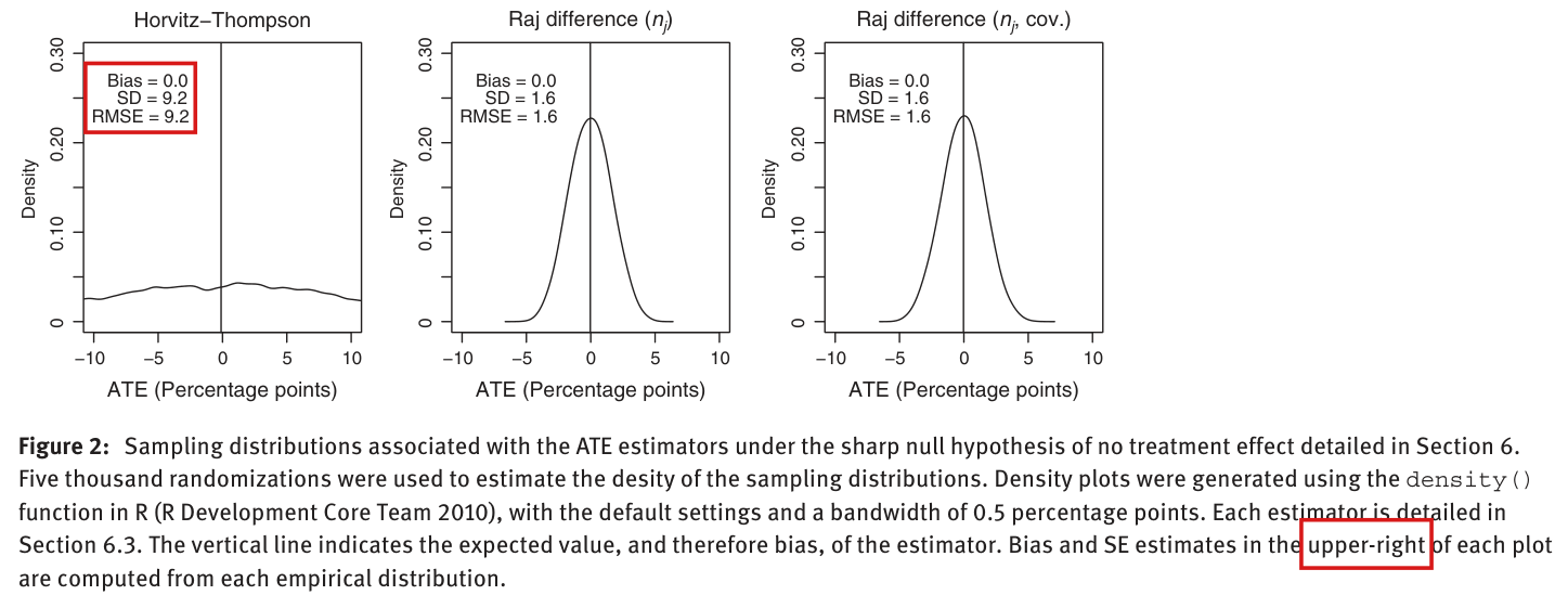
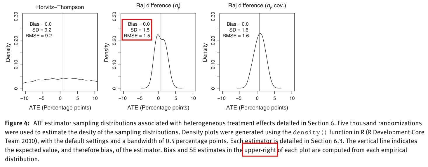
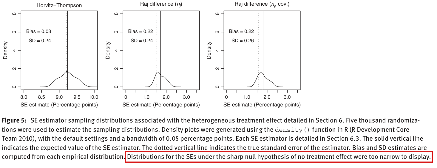
In Figures 2 and 4 the labels are in the upper left of each panel, not the upper right, and the last sentence of the caption of Figure 5 belongs to Figure 3.

Captions of Figure 2, p. 64 (PDF p. 26), Figure 4, p. 67 (PDF p. 29), and Figure 5, p. 69 (PDF p. 31)

As printed

Captions of Figures 2 and 4: “Bias and SE estimates in the upper-right of each plot are computed from each empirical distribution.”

Caption of Figure 5, last sentence: “Distributions for the SEs under the sharp null hypothesis of no treatment effect were too narrow to display.”

The problem

Every panel of Figures 2 and 4 carries its labels (Bias, SD and RMSE) in the upper left. Figure 5 shows the scenario with heterogeneous effects and displays all seven distributions of standard errors. Its last sentence repeats a remark from the caption of Figure 3. That figure concerns the sharp-null scenario, and the distributions for its three design-based estimators are omitted.

Evidence a check of the printed page

The evidence is a check of the pages: Figures 2 to 5 were inspected upright, panel by panel.

What survives

The panels and their numbers are unaffected. The sentence about the sharp null is true of Figure 3, whose caption already contains it. Naming the three labels in the corrected caption is optional, since “SE” is acceptable usage for the standard deviation of a point estimator.

Corrected

Captions of Figures 2 and 4: “Bias, SD, and RMSE summaries in the upper-left of each plot are computed from each empirical distribution.”

Caption of Figure 5: the caption ends with “Bias and SD estimates are computed from each empirical distribution.” Distributions for the SEs under the sharp null hypothesis of no treatment effect were too narrow to display.

Crop of the three design-based panels of Figure 2 and its caption. One red box marks the word 'upper-right' in the last sentence of the caption. A second red box marks the labels Bias = 0.0, SD = 9.2, RMSE = 9.2, which sit in the upper left corner of the Horvitz-Thompson panel. The other two panels carry their labels in the upper left as well.
Figure 2, p. 64 (PDF p. 26), lower row of panels and caption, turned upright. The caption places the labels in the upper right of each plot (the word is marked). They are in the upper left, as the marked labels of the first panel show.
Crop of the three design-based panels of Figure 4 and its caption. One red box marks the word 'upper-right' in the caption. A second red box marks the labels Bias = 0.0, SD = 1.5, RMSE = 1.5 in the upper left corner of the panel 'Raj difference (n j)'.
Figure 4, p. 67 (PDF p. 29), lower row of panels and caption, turned upright. The same sentence appears (the word “upper-right” is marked), and the labels are again in the upper left, as marked in the second panel.
Crop of the three design-based panels of Figure 5 and its caption. A red box marks the last sentence of the caption, 'Distributions for the SEs under the sharp null hypothesis of no treatment effect were too narrow to display.' Each of the three panels above it shows a density curve with a solid and a dotted vertical line.
Figure 5, p. 69 (PDF p. 31), lower row of panels and caption, turned upright. The marked sentence says that distributions under the sharp null were too narrow to display; Figure 5 shows the scenario with heterogeneous effects, and every panel has its distribution.

On p. 52 the two facts under the sharp null should be written for the cluster totals Y0jTY^T_{0j}, Y1jTY^T_{1j} and YjTY^T_j, the subscript of Y0iY_{0i} is broken, and “ncn_c or ntn_t” should read “mcm_c or mtm_t”.

Section 4.2, first two lines of p. 52 (PDF p. 14) and the paragraph beginning “The primary benefit of using”

See also under Formal statements (Lean): P020-T10

As printed

“identical: Y0i=Y1i=Yi\colorbox{#ffe58a}{$Y_0i$}=Y_{1i}=Y_i. When the sharp null hypothesis of no effect holds, we know two important facts: σ2(Y0j)=σ2(Y1j)=σ2(Yj)\colorbox{#ffe58a}{$\sigma^2(Y_{0j})=\sigma^2(Y_{1j})=\sigma^2(Y_j)$} and σ(Y0j,Y1j)=σ2(Yj)\colorbox{#ffe58a}{$\sigma(Y_{0j},Y_{1j})=\sigma^2(Y_j)$}.”

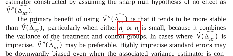
“The primary benefit of using V^N(ΔHT^)\hat{\mathrm{V}}^N(\widehat{\Delta_{HT}}) is that it tends to be more stable than V^(ΔHT^)\hat{\mathrm{V}}(\widehat{\Delta_{HT}}), particularly when either nc\colorbox{#ffe58a}{$n_c$} or nt\colorbox{#ffe58a}{$n_t$} is small, because it combines the variance of the treatment and control groups.”

The problem

The variances that enter equation (17), and the display that follows these lines on p. 52, are variances of cluster totals: Y0jTY^T_{0j} and Y1jTY^T_{1j} are defined on p. 48 and their variances on p. 50. Without the superscript the symbols Y0jY_{0j}, Y1jY_{1j} and YjY_j are not defined. In Y0iY_0i the index ii is printed on the baseline. The symbols ncn_c and ntn_t denote the numbers of individuals in the control and treatment arms (p. 44), which are random under the assignment of clusters. The estimator V^(ΔHT^)\hat{\mathrm{V}}(\widehat{\Delta_{HT}}) has the denominators mc(mc−1)m_c(m_c-1) and mt(mt−1)m_t(m_t-1) and is undefined when mcm_c or mtm_t is 11 (p. 51). Its stability therefore depends on the number of clusters in each arm.

Evidence a check of the printed page

The evidence is a check of the page against the definitions on pp. 44, 48, 50 and 51. The display that follows the two facts on p. 52 writes σ2(YjT)\sigma^2(Y^T_j).

What survives

Equation (17), the display for VN(ΔHT^)\mathrm{V}^N(\widehat{\Delta_{HT}}) and the remark on stability are correct with these readings. Under the sharp null the identities hold for the cluster totals as they do for the individual outcomes. Nothing else changes.

Corrected

“identical: Y0i=Y1i=Yi\colorbox{#ffe58a}{$Y_{0i}$}=Y_{1i}=Y_i. … two important facts: σ2(Y0jT)=σ2(Y1jT)=σ2(YjT)\sigma^2(\colorbox{#ffe58a}{$Y^T_{0j}$})=\sigma^2(\colorbox{#ffe58a}{$Y^T_{1j}$})=\sigma^2(\colorbox{#ffe58a}{$Y^T_j$}) and σ(Y0jT,Y1jT)=σ2(YjT)\sigma(\colorbox{#ffe58a}{$Y^T_{0j}$},\colorbox{#ffe58a}{$Y^T_{1j}$})=\sigma^2(\colorbox{#ffe58a}{$Y^T_j$}).”

“The primary benefit of using V^N(ΔHT^)\hat{\mathrm{V}}^N(\widehat{\Delta_{HT}}) is that it tends to be more stable than V^(ΔHT^)\hat{\mathrm{V}}(\widehat{\Delta_{HT}}), particularly when either mc\colorbox{#ffe58a}{$m_c$} or mt\colorbox{#ffe58a}{$m_t$} is small, because it combines the variance of the treatment and control groups.”

Crop of the opening lines of the page. Red boxes mark 'Y_0 i = Y_1i = Y_i', in which the i of the first symbol sits on the baseline, and the two identities 'sigma squared of Y_0j = sigma squared of Y_1j = sigma squared of Y_j' and 'sigma of Y_0j, Y_1j = sigma squared of Y_j', none of which carries a superscript T.
First lines of p. 52 (PDF p. 14). The marked symbols are the broken subscript in Y0iY_{0i} and the two facts, printed without the superscript TT of a cluster total.
Crop of the paragraph. A red box marks 'n_c or n_t' in 'it tends to be more stable than V-hat of Delta-hat-HT, particularly when either n_c or n_t is small, because it combines the variance of the treatment and control groups'.
Paragraph beginning “The primary benefit of using”, p. 52 (PDF p. 14). The marked symbols are the numbers of individuals in the two arms; the numbers of clusters mcm_c and mtm_t are meant.

“Three commonly used estimators” should read “four”, and the turnout covariate is measured for the cable district and is not “precinct-level”.

Section 6.1, last paragraph, p. 60 (PDF p. 22); Section 6.3, p. 62 (PDF p. 24)

As printed

p. 60: “We use randomization inference to examine the behavior of our estimators and compare them with the behavior of three commonly used estimators.”

p. 62: “where β2\beta_2 is the coefficient on precinct-level voter turnout in 2000, β3\beta_3 is the coefficient on age, and the model is fitted with ordinary least squares.”

The problem

Section 6.3 opens with “We will consider four regression-based estimators as well as the three design-based estimators proposed in this paper” (p. 61). It defines four regression estimators, and each of Figures 2–5 has four regression panels. The turnout covariate is defined on p. 59 as the “turnout rate in the cable district in the 2000 election”. The clusters are cable districts, and the turnout covariate is defined at that level.

Evidence a check of the printed page

I checked pp. 59–63 and the panels of Figures 2–5.

What survives

The estimators that are compared are those of Section 6.3 and the figures, and no number changes. The two covariates are indexed X2X_2, X3X_3 in the regressions (p. 62) and X1TX^T_1, X2TX^T_2 in the Des Raj model (p. 63). Each model defines its own indices, and this is not an error.

Corrected

p. 60: “… compare them with the behavior of four commonly used estimators.”

p. 62: “where β2\beta_2 is the coefficient on the cable-district turnout rate in 2000, β3\beta_3 is the coefficient on age, and the model is fitted with ordinary least squares.”

Crop of the last paragraph of Section 6.1. A red box marks the word 'three' in 'We use randomization inference to examine the behavior of our estimators and compare them with the behavior of three commonly used estimators.'
Section 6.1, last paragraph, p. 60 (PDF p. 22). The marked word gives the number of comparison estimators as three; Section 6.3 defines four.
Crop of the fixed-effects regression with covariates and the sentence below it. A red box marks 'precinct-level' in 'where beta_2 is the coefficient on precinct-level voter turnout in 2000, beta_3 is the coefficient on age'.
Section 6.3, p. 62 (PDF p. 24). The marked word places the turnout covariate at the level of the precinct; p. 59 defines it as the turnout rate in the cable district.

Section 6.3 states a standard-error procedure for every estimator except the regression without covariates of equation (27); the procedure used for that regression needs to be stated, and ordinary least-squares standard errors cannot explain the figure on whole-cluster subsets of the public data.

Section 6.3, p. 62 (PDF p. 24), paragraph beginning “As Freedman (2008a) notes”; equation (27), p. 61 (PDF p. 23); Figure 3, p. 65 (PDF p. 27)

As printed

Section 6.3, p. 61, after equation (27): “Our estimate of β1\beta_1 follows from fitting the model with ordinary least squares.”

Section 6.3, p. 62: “For both fixed effects models, Huber-White “robust” cluster standard errors are estimated.”

Section 6.4, pp. 63 and 66: “In the case of the regression with no covariates (difference-in-means) the standard errors are biased upwards due to the failure of this model to account for blocking.”

The problem

Section 6.3 specifies the standard errors of the two fixed-effects regressions (cluster-robust), of the random-effects regression (produced by lmer()) and of the three design-based estimators (the square root of the estimated variance under the sharp null). For the first regression, equation (27), it says only that the coefficient is fitted by ordinary least squares. Figures 3 and 5 nevertheless show a distribution of standard errors for this regression, and Section 6.4 interprets its upward bias. The paper does not say which standard error was computed, and the procedure cannot be recovered from the article or from the scripts of the source study, which serve a different analysis.

Evidence a recalculation from the source

The evidence is a check of the pages and a recalculation from the public data of the source study. Figure 3 reports a bias of 0.53 percentage points for this panel, measured from the standard deviation of the estimator, which Figure 2 reports as 2.4. Then the mean of the plotted standard errors is about 2.93 points. On whole-cluster subsets of the public data, the standard error from ordinary least squares cannot be that large. For a binary outcome regressed on a constant and a treatment indicator, the residual sum of squares is at most N/4N/4, so that the residual variance satisfies s2≤N/(4(N−2))s^2\le N/(4(N-2)). With ntn_t and ncn_c individuals in the two arms, the squared standard error of β^1\hat\beta_1 is s2(1/nt+1/nc)s^2(1/n_t+1/n_c). Each arm consists of 40 whole clusters, and in the public data the 40 smallest of the 85 clusters contain L=5,654L=5{,}654 individuals together, so that each arm has at least LL individuals. I have

s2(1nt+1nc)≤N4(N−2)(1L+1N−L).s^2\Bigl(\frac{1}{n_t}+\frac{1}{n_c}\Bigr)\le\frac{N}{4(N-2)}\Bigl(\frac{1}{L}+\frac{1}{N-L}\Bigr).

With N=22,733N=22{,}733 the square root of the right side gives a bound of about 0.7670.767 percentage points, for every assignment under these assumptions. This rules out ordinary least-squares standard errors for that sample construction. It does not identify the procedure or establish that the authors used the public data unchanged.

What survives

The point estimators as displayed and the labels printed in the figures stand. No standard-error implementation and no design-based formula is shown to be wrong. The distributions of the regression standard errors and the comparisons of their biases cannot be reproduced exactly.

Corrected

“For both fixed effects models, Huber-White “robust” cluster standard errors are estimated. For the regression without covariates, the standard errors are computed by [the procedure that was used].”

The added sentence cannot be completed from the article or from the replication files of the source study. For each robust standard error, the description should also give the clustering variable, the covariance formula, the finite-sample correction and the treatment of the blocks.

Crop of a paragraph of Section 6.3. Red boxes mark the sentence 'For both fixed effects models, Huber-White robust cluster standard errors are estimated', which runs over two lines. The sentences before it discuss bias from regression adjustment, and the sentence after it says that these standard errors may be unreliable in finite samples.
Section 6.3, p. 62 (PDF p. 24). The marked sentence is the only statement of a standard-error procedure for the least-squares regressions, and it covers the two fixed-effects models only.

Clarity notes

Imprecise or ambiguous wording whose intended meaning is correct; not an error.

Read literally, two sentences say that the difference in means is biased whenever cluster size is related to outcomes; the meaning is that such a relation can bias it, and by equation (8) the terms of the two arms can cancel.

Section 3.2, the sentence after equation (8) and the paragraph that follows, p. 45 (PDF p. 7); first sentence of p. 44 (PDF p. 6)

See also under Formal statements (Lean): P020-T11

As printed

p. 44: “As our derivation will show, the bias arises whenever outcomes are related to cluster size.”

p. 45: “Inspection of this term reveals that, if the size of the cluster is correlated with the potential outcomes in the cluster, the difference-in-means estimator is biased. Moreover, the presence of the terms 1/mt1/m_t and 1/mc1/m_c shows that the magnitude (and even the direction) of the bias can depend on the relative number of clusters allocated to treatment and control.

In some special cases, there will be no bias, such as when the cluster size does not vary or when there is no covariance between cluster size and outcomes.”

Intended meaning

The passage warns that the difference in means is not unbiased in general when cluster size is related to outcomes. The warning is correct, and equation (8) and the paragraph on special cases state the exact condition. I write R1R_1 and R0R_0 for the mean outcomes of the treated and the control individuals under a given assignment, and ntn_t and ncn_c for the numbers of treated and control individuals. Then equation (8) reads

E[ΔS^]−Δ=−MN[Cov⁡(R1,nt)mt−Cov⁡(R0,nc)mc],\mathrm{E}[\widehat{\Delta_S}]-\Delta=-\frac{M}{N}\left[\frac{\operatorname{Cov}(R_1,n_t)}{m_t}-\frac{\operatorname{Cov}(R_0,n_c)}{m_c}\right],

which implies that the bias is zero exactly when the two terms in the bracket are equal. The words “whenever” and “is biased” claim more than this. For example, let M=2M=2 and mt=mc=1m_t=m_c=1, and suppose that the first cluster has one individual with Y0=Y1=0Y_0=Y_1=0 and the second has two individuals with Y0=Y1=1Y_0=Y_1=1. The outcomes are perfectly correlated with cluster size, and both covariances equal 1/41/4. The estimator takes the values −1-1 and 11 with probability 1/21/2 each, and its expectation is 0=Δ0=\Delta. In a second example the arms have unequal numbers of clusters (M=3M=3, mt=1m_t=1, sizes 11, 22, 33), and the effects are positive and vary with cluster size. There Δ=44/45\Delta=44/45, each arm mean has bias −7/90-7/90, and the difference in means is unbiased. The balanced design under the sharp null in Section 6.4, for which the paper reports no bias, is another case of cancellation.

Note that equation (8) is correct as printed, including its sign, and that the estimator can be biased: with sizes (1,2)(1,2), control means (0,1)(0,1) and treatment means (0,2)(0,2) in the two clusters, its bias is −1/6-1/6. In the clause “no covariance between cluster size and outcomes”, the covariances are the two in equation (8). No estimator, derivation or reported number depends on the stronger wording.

Corrected

p. 44: “… bias can arise when outcomes are related to cluster size.”

p. 45: “Inspection of this term reveals that, if the size of the cluster is correlated with the potential outcomes in the cluster, the difference-in-means estimator can be biased. The terms of the two arms in equation (8) can cancel, and the estimator is unbiased exactly when they are equal. Moreover, the presence of the terms 1/mt1/m_t and 1/mc1/m_c shows that the magnitude (and even the direction) of the bias can depend on the relative number of clusters allocated to treatment and control.

In some special cases, there will be no bias, such as when the cluster size does not vary or when both covariances in equation (8) are zero.”

Crop of equation (8), which gives the bias as minus M over N times the difference of two covariance terms divided by m_t and m_c, and of the lines after it. A red box marks the words 'is biased.' at the end of the sentence 'if the size of the cluster is correlated with the potential outcomes in the cluster, the difference-in-means estimator is biased.' The next paragraph begins 'In some special cases, there will be no bias'.
Equation (8) and the sentences after it, p. 45 (PDF p. 7). The marked words state as certain a bias that equation (8) makes possible.
Crop of the first lines of the page. A red box marks the words 'the bias arises whenever' in the sentence 'As our derivation will show, the bias arises whenever outcomes are related to cluster size.'
First lines of p. 44 (PDF p. 6). The marked words announce the same condition before the derivation.

The formulas for the optimal kk presuppose that the cluster sizes are not all equal, σ2(nj)>0\sigma^2(n_j)>0, and the informal summary on p. 57 leaves out the cases k=0k=0 and k=2koptim∗k=2k_{\mathit{optim}*}, in which the two variances are equal.

Section 5.3: last paragraph of p. 56 (PDF p. 18), leading to equation (26); paragraph beginning “The chosen value of kk”, p. 57 (PDF p. 19)

See also under Formal statements (Lean): P020-T14

As printed

pp. 56–57: “Since the second derivative with respect to kk, 2σ2(nj)2\sigma^2(n_j), must be positive, we may set the first derivative equal to zero and solve for kk, so that” and then equation (26),

koptimc=σ(nj,Y0jT)σ2(nj).k_{\mathit{optim}_c}=\frac{\sigma(n_j,Y^T_{0j})}{\sigma^2(n_j)}.

p. 57: “The chosen value of kk will reduce the variability of the Des Raj estimator, ΔR1^\widehat{\Delta_{R1}}, relative to the HT estimator when, for koptim∗>0k_{\mathit{optim}*}>0, 0<k<2koptim∗0<k<2k_{\mathit{optim}*} and, for koptim∗<0k_{\mathit{optim}*}<0, 0>k>2koptim∗0>k>2k_{\mathit{optim}*}. In other words, the Des Raj estimator will have better precision than the HT estimator unless the researcher picks a kk with the wrong sign or chooses a kk that is more than twice the magnitude of koptim∗k_{\mathit{optim}*}.”

Intended meaning

Section 5 concerns clusters of unequal size, and for these the formulas are correct. I write V(k)\mathrm{V}(k) for the variance of the Des Raj estimator with a fixed kk, so that V(0)\mathrm{V}(0) is the variance of the Horvitz–Thompson estimator. Let c=(M−mc)/mcc=(M-m_c)/m_c, t=(M−mt)/mtt=(M-m_t)/m_t and v=(M−1)N2/M2v=(M-1)N^2/M^2, as in Appendix C. By the expansion in Appendix C, I have

v [V(k)−V(0)]=(c+t+2) σ2(nj) k (k−2koptim∗),koptim∗=mtMkoptimc+mcMkoptimt.v\,[\mathrm{V}(k)-\mathrm{V}(0)]=(c+t+2)\,\sigma^2(n_j)\,k\,(k-2k_{\mathit{optim}*}),\qquad k_{\mathit{optim}*}=\frac{m_t}{M}k_{\mathit{optim}_c}+\frac{m_c}{M}k_{\mathit{optim}_t}.

When σ2(nj)>0\sigma^2(n_j)>0 the variance has a unique minimum at koptim∗k_{\mathit{optim}*}, and the Des Raj estimator has the smaller variance exactly when k(k−2koptim∗)<0k(k-2k_{\mathit{optim}*})<0. These are the strict intervals that the paper prints before the marked sentence. The two variances are equal at k=0k=0 and at k=2koptim∗k=2k_{\mathit{optim}*}, and when koptim∗=0k_{\mathit{optim}*}=0 no nonzero kk improves on the Horvitz–Thompson estimator. For example, let M=4M=4 and mt=2m_t=2, with sizes (1,2,3,4)(1,2,3,4), control totals (3,3,5,9)(3,3,5,9) and a constant effect of 11 on the totals. Then koptim∗=2k_{\mathit{optim}*}=2, and the variance is 1.281.28 at k=0k=0, 0.21330.2133 at k=2k=2 and 1.281.28 at k=4k=4.

When all clusters have the same size, nj−N/M=0n_j-N/M=0 for every jj. The adjustment then vanishes, the Des Raj estimator coincides with the Horvitz–Thompson estimator for every kk, and the quotients in equation (26) and in Appendix C are 0/00/0. The Des Raj estimator remains unbiased in that case. Nothing in the paper depends on the two omissions.

Corrected

pp. 56–57: “Assume that the cluster sizes are not all equal, so that σ2(nj)>0\sigma^2(n_j)>0. Since the second derivative with respect to kk, 2σ2(nj)2\sigma^2(n_j), is then positive, … If all clusters have the same size, the adjustment vanishes and every kk gives the HT estimator.”

p. 57: “In other words, the Des Raj estimator will have better precision than the HT estimator when kk lies strictly between 00 and 2koptim∗2k_{\mathit{optim}*}. The two estimators have the same precision at k=0k=0 and at k=2koptim∗k=2k_{\mathit{optim}*}, and when koptim∗=0k_{\mathit{optim}*}=0 no nonzero kk improves on the HT estimator.”

Crop of the last four lines of the page. A red box marks '2 sigma squared of n_j, must be positive,' in the sentence 'Since the second derivative with respect to k, 2 sigma squared of n_j, must be positive, we may set the first derivative equal to zero and solve for k, so that'.
Section 5.3, last lines of p. 56 (PDF p. 18). The marked words assert that 2σ2(nj)2\sigma^2(n_j) is positive, which holds when the cluster sizes are not all equal.
Crop of the paragraph beginning 'The chosen value of k will reduce the variability of the Des Raj estimator'. Red boxes mark 'will have better precision than' and, on the next line, 'the HT estimator unless' in the sentence 'In other words, the Des Raj estimator will have better precision than the HT estimator unless the researcher picks a k with the wrong sign or chooses a k that is more than twice the magnitude of k_optim*.' The sentence before gives the intervals 0 < k < 2 k_optim* and 0 > k > 2 k_optim*.
Section 5.3, p. 57 (PDF p. 19). The strict intervals are printed in the sentence before; the marked summary omits the boundary cases.

“Will have a higher value than that of the true variance” is meant in expectation: under the stated conditions the sharp-null variance estimator has nonnegative bias, and the estimate from one assignment can fall below the true variance.

Section 4.2, paragraph beginning “Recent theoretical results suggest”, p. 52 (PDF p. 14)

See also under Formal statements (Lean): P020-T16

As printed

“In general, V^N(ΔHT^)\hat{\mathrm{V}}^N(\widehat{\Delta_{HT}}) will be conservative relative to the true variance if effects are constant (at the cluster scale) or if the number of clusters is balanced, in a result that directly follows from theorem 3 of Ding (2014) and Samii and Aronow (2012) (by way of the relationship between pooled and combined variance). These results indicate V^N(ΔHT^)\hat{\mathrm{V}}^N(\widehat{\Delta_{HT}}) will have a higher value than that of the true variance if treatment effects are in fact constant at the cluster scale.”

Intended meaning

On p. 51 the paper calls a variance estimator conservative when its bias is nonnegative. The marked sentence restates that property for the sharp-null variance estimator: its expectation over the assignments is at least the true variance. The property holds. Let dj=Y1jT−Y0jTd_j=Y^T_{1j}-Y^T_{0j} denote the effect on the total of cluster jj, with mean d‾\overline{d} and variance σ2(d)\sigma^2(d) over the MM clusters. Using equation (17) and the closed form of the estimator on p. 52, I obtain

E[V^N(ΔHT^)]−V(ΔHT^)=M2N2(M−1) τ2≥0\mathrm{E}[\hat{\mathrm{V}}^N(\widehat{\Delta_{HT}})]-\mathrm{V}(\widehat{\Delta_{HT}})=\frac{M^2}{N^2(M-1)}\,\tau^2\ge0

when dj=τd_j=\tau for every cluster, and

E[V^N(ΔHT^)]−V(ΔHT^)=M2N2(M−1)[d‾ 2+M−2M−1 σ2(d)]≥0\mathrm{E}[\hat{\mathrm{V}}^N(\widehat{\Delta_{HT}})]-\mathrm{V}(\widehat{\Delta_{HT}})=\frac{M^2}{N^2(M-1)}\left[\overline{d}^{\,2}+\frac{M-2}{M-1}\,\sigma^2(d)\right]\ge0

when mt=mcm_t=m_c. Note that the inequality is weak: equality holds under the sharp null. The estimate from a single assignment can be smaller than the true variance. For example, let M=N=4M=N=4 and mt=mc=2m_t=m_c=2, with control totals (0,0,2,2)(0,0,2,2) and a constant effect of 22. Then the true variance is 4/34/3, and the estimator has mean 8/38/3 over the six assignments. When the first two clusters are treated, each of the four observed totals equals 22 and the estimate is 00. Here “constant at the cluster scale” means a constant effect on the cluster totals. Nothing in the paper depends on the wording.

Corrected

“Under constant cluster-total treatment effects or balanced cluster counts, E[V^N(ΔHT^)]≥V(ΔHT^)\colorbox{#ffe58a}{$\mathrm{E}[\hat{\mathrm{V}}^N(\widehat{\Delta_{HT}})]\ge\mathrm{V}(\widehat{\Delta_{HT}})$}; the realized estimate need not exceed the true variance.”

Crop of the paragraph beginning 'Recent theoretical results suggest'. Red boxes mark the words 'will have a higher value' and, on the next line, 'than that of the true variance' in the sentence 'These results indicate V-hat-N of Delta-hat-HT will have a higher value than that of the true variance if treatment effects are in fact constant at the cluster scale.' The sentence before says the estimator 'will be conservative relative to the true variance if effects are constant (at the cluster scale) or if the number of clusters is balanced'.
Section 4.2, p. 52 (PDF p. 14). The marked words describe the estimate itself as higher than the true variance; the property that holds is the one in the sentence before, that the estimator is conservative.

Formal statements (Lean)

Formal results: 16 whole; 1 restricted; 0 refuted; 0 omitted.

Coverage concerns the identified claim under its stated assumptions. A checked proof establishes the formal statement; correspondence to the published text was reviewed by AI. Repository access is currently required to open the source links.

Each result links to its current formal statement and proof. “Whole” covers the identified claim under its assumptions; “restricted” covers the stated narrower scope; “refuted” gives a counterexample to the identified assertion; “omitted” has no current theorem. Any named published theorem used as a premise remains an assumption. Browse the formal results for this work.

Introduction, unnumbered sentence 'Estimators that are asymptotically biased are guaranteed to be relatively inefficient for a sufficiently large sample size'; repeated in the opening paragraph of Section 3

p. 40 (PDF p. 2); p. 42 (PDF p. 4)

p. 40 (PDF p. 2); p. 42 (PDF p. 4). The explicit three-cluster population has persistent bias and probability-one error, yet its difference in means beats HT and every fixed-coefficient Des Raj estimator at every positive within-cluster replication.

Historical component credits
  • Proved AronowAudit.P020.efficiency_individual_realization Historical support retained; baseline fidelity: ok; manifest: used; used in Solution; Fidelity sweep: ok
  • Proved AronowAudit.P020.efficiency_exact_values Historical support retained; baseline fidelity: ok; manifest: used; used in Solution; Fidelity sweep: ok
  • Proved AronowAudit.P020.efficiency_raj_mse Historical support retained; baseline fidelity: ok; manifest: used; used in Solution; The lower bound follows from the exported completed-square equality with coefficient 9/14>0; it is not hidden in a hypothesis.
  • Proved AronowAudit.P020.efficiency_optimal_coefficient Historical support retained; baseline fidelity: ok; manifest: used; used in Solution; Fidelity sweep: ok
  • Counterexample proved AronowAudit.P020.efficiency_mse_counterexample Historical support retained; baseline fidelity: ok; manifest: used; used in Solution; Des Raj at k=0 is HT by expansion of rajPotential and desRaj, so the universally quantified estimator inequality includes the HT comparison.
  • Proved AronowAudit.P020.efficiency_error_probability Historical support retained; baseline fidelity: ok; manifest: used; used in Solution; Fidelity sweep: ok
  • Counterexample proved AronowAudit.P020.efficiency_all_replications_counterexample Historical support retained; baseline fidelity: ok; manifest: used; used in Solution; Witness family for the printed blanket guarantee relative to HT and all fixed-k Des Raj estimators, not a claim of dominance over every unbiased estimator; k may depend on h but not the realized assignment. T1 is marked asymptotic=false although clause (v) includes N_h tending to infinity and inconsistency.
  • Proved AronowAudit.P020.efficiency_sample_size_grows Historical support retained; baseline fidelity: ok; manifest: used; used in Solution; This is an auxiliary scalar size-growth fact, used with the explicit population-size equality in R138-01, not an estimator assertion on its own.
  • Proved AronowAudit.P020.efficiency_inconsistent Historical support retained; baseline fidelity: ok; manifest: used; used in Solution; {'source': 'adjudication', 'decision': 'rejected', 'what': "P020/P020_Design.lean:2664 states nonconvergence for the original E001 law, statistic, and ATE, which is equivalent to the T1(v) component that the estimator is not consistent along the within-cluster replication sequence. The population at P020/P020_Design.lean:2495 has exactly the target's sizes (1,2,4) and potential totals (0,1,1) and (0,0,0), and the resulting estimator values (-1/3,-1/5,-1/3) all differ from -2/7 by more than 1/25. The statements at P020/P020_Design.lean:2619 and :2395 identify the replicated statistic, target, and law with the original ones for every positive h and give error probability one and N_h=7h; :2655 states that this size tends to infinity. Thus the constant-law expression preserves the complete error distribution along the actual growing populations, and the unused h=0 index does not affect convergence at infinity."}

Introduction, unnumbered sentence 'Estimators that are asymptotically biased are guaranteed to be relatively inefficient ...' (and the Section 3 roadmap sentence), as corrected

p. 40 (PDF p. 2); p. 42 (PDF p. 4)

p. 40 (PDF p. 2); p. 42 (PDF p. 4). Finite-law MSE decomposes into variance and squared bias, nonzero limiting bias implies eventual inferiority to a vanishing-MSE comparator, and a Markov bound gives consistency from vanishing MSE, with a counterexample when the comparator condition is dropped.

Historical component credits
  • Proved AronowAudit.P020.mse_bias_variance Historical support retained; baseline fidelity: ok; manifest: used; used in Solution; The larger domain strengthens T2(a); finite support makes all moments finite without adding a restriction to the paper's finite design.
  • Proved AronowAudit.P020.squared_bias_le_mse Historical support retained; baseline fidelity: ok; manifest: used; used in Solution; The larger domain strengthens the lower-bound component of T2(a); no bias or MSE conclusion is stored in FiniteLaw.
  • Proved AronowAudit.P020.mse_markov_bound Historical support retained; baseline fidelity: ok; manifest: used; used in Solution; The strict error event and positive epsilon match T2(c); epsilon positivity excludes zero division.
  • Proved AronowAudit.P020.eventual_mse_inferiority Historical support retained; baseline fidelity: ok; manifest: used; used in Solution; The larger domain is harmless and strengthens the corrected claim; the two convergence premises and b!=0 are precisely the corrected hypotheses rather than assumed intermediate results.
  • Proved AronowAudit.P020.vanishing_mse_consistent Historical support retained; baseline fidelity: ok; manifest: used; used in Solution; The larger domain strengthens T2(c); h=0 is an irrelevant initial index and convergence is through the entire natural tail.

Section 6.2, logistic regression model (unnumbered display) with the sentences 'We estimate tau as 0.4, beta as 1.4 and phi as -0.9' and 'the ATE is in expectation ... = 0.007'

p. 61 (PDF p. 23); definition of n_j on p. 44 (PDF p. 6)

p. 61 (PDF p. 23); definition of n_j on p. 44 (PDF p. 6). The printed logistic link is strictly increasing, and the raw-count treatment shift 2/5 - (9/10)n is at most -1/2 for every real n at least one. Consequently every individual probability contrast and every finite nonempty average contrast is negative, excluding the reported 7/1000, for arbitrary real control predictors and sizes at least one. The scalar instance N = 1, n = 1, control predictor zero has control probability 1/2 and treated probability L(-1/2) < 1/2. The usual measure-theoretic conditions are assumed; the displayed quantities are finite real expressions. The scalar instance specifies no randomized cluster design.

Historical component credits
  • Proved AronowAudit.P020.logistic_strictMono Historical support retained; baseline fidelity: ok; manifest: used; used in Solution; Fidelity sweep: ok
  • Proved AronowAudit.P020.printed_contrast_bound Historical support retained; baseline fidelity: ok; manifest: used; used in Solution; The target explicitly states this auxiliary bound for real n>=1, so there is no additional domain mismatch in this component.
  • Proved AronowAudit.P020.printed_model_unit_negative Historical support retained; baseline fidelity: ok; manifest: used; used in Solution; The real-size generalization preserves the sign conclusion for every integer cluster count; the fixed beta and block terms are absorbed into the universally quantified baseline.
  • Counterexample proved AronowAudit.P020.printed_model_average_negative Historical support retained; baseline fidelity: ok; manifest: used; used in Solution; The stronger-domain sign theorem includes all actual printed-model predictors and cluster counts, so no admissible population is excluded.
  • Counterexample proved AronowAudit.P020.printed_model_average_ne_reported Historical support retained; baseline fidelity: ok; manifest: used; used in Solution; This is a full universal impossibility argument, not a purported single-population witness: substitute the actual control predictors and integer cluster counts to exclude the printed positive average. Decimal coefficients and 0.007 are treated as the exact printed rationals.
  • Counterexample proved AronowAudit.P020.logistic_concrete_counterexample Historical support retained; baseline fidelity: ok; manifest: used; used in Solution; The scalar illustration does not supply an admissible N=1 randomized cluster population under the standing arm-count assumptions.

Section 6.2, logistic regression model (unnumbered display), with the scale of the cluster-size predictor stated

p. 61 (PDF p. 23)

p. 61 (PDF p. 23). Conditionally replacing cluster size by its value in thousands gives the equivalent raw-count slopes and the stated real, integer, probability and average sign thresholds.

Historical component credits
  • Proved AronowAudit.P020.repaired_scale_equivalence Historical support retained; baseline fidelity: ok; manifest: used; used in Solution; The block term is arbitrary, so every finite sum of block fixed effects is included; beta=1.4 and phi=-0.9 on n/1000 give exactly 0.0014 and -0.0009 on n.
  • Proved AronowAudit.P020.repaired_real_sign Historical support retained; baseline fidelity: ok; manifest: used; used in Solution; The real threshold and integer cutoff are complementary components of T4; there is no loss at the real zero-contrast boundary.
  • Proved AronowAudit.P020.repaired_integer_sign Historical support retained; baseline fidelity: ok; manifest: used; used in Solution; The added zero-count case is harmless; positive counts specialize the theorem exactly. No published theorem is assumed as a premise.
  • Proved AronowAudit.P020.repaired_probability_sign Historical support retained; baseline fidelity: ok; manifest: used; used in Solution; Logistic denominators are always positive, and monotonicity preserves the required treatment contrast signs.
  • Proved AronowAudit.P020.repaired_average_sign Historical support retained; baseline fidelity: ok; manifest: used; used in Solution; This is the explicitly conditional scale repair, not a claim to recover the historical units or reproduce 0.007. The two homogeneous-size premises are separate implications; neither promises a sign for mixed sizes.

Appendix B, equation (31), with equations (29)-(30); the same formula is printed unnumbered at the end of p. 57 in Section 5.3

pp. 70-71 (PDF pp. 32-33); p. 57 (PDF p. 19) and p. 58 (PDF p. 20)

Appendix B, pp. 70-71 (PDF pp. 32-33); pp. 57-58 (PDF pp. 19-20). For every coefficient estimated from the same experiment, both complete arm-total expectation calculations (29)-(30) hold, and the corrected ATE expectation is Delta plus M/N times (control covariance minus treatment covariance), while the bias equals that covariance correction.

Historical component credits
  • Proved AronowAudit.P020.estimated_raj_total_mean Historical support retained; baseline fidelity: ok; manifest: used; used in Solution; Supporting row is already assembled into the selected primary declarations; it is not invoked separately.
  • Proved AronowAudit.P020.estimated_coefficient_bias Historical support retained; baseline fidelity: ok; manifest: used; used in Solution; Finite assignment space supplies all moments without an extra integrability premise. Only the corrected (31), with the treatment-size covariance in the second position, is credited.

Appendix B, equation (31) as printed

p. 71 (PDF p. 33)

p. 71 (PDF p. 33). The explicit nondegenerate OLS witness has mean one eighth instead of one half and bias minus three eighths, with the assignment values and both covariances in the corrected formula.

Historical component credits
  • Counterexample proved AronowAudit.P020.estimated_slope_counterexample Historical support retained; baseline fidelity: ok; manifest: used; used in Solution; This is an exact witness against the printed universally zero bias term; the OLS denominator is positive. The immediate cancellation x-x=0 requires no stronger interpretation of printed (31).

Section 5.2, equations (24)-(25): invariance of the Des Raj difference estimator

pp. 55-56 (PDF pp. 17-18); transformation defined on p. 49 (PDF p. 11)

pp. 55-56 (PDF pp. 17-18); transformation defined on p. 49 (PDF p. 11). Individual affine transformation and the matching coefficient transformation give both potential-total identities and all nondefinitional equalities of the corrected Des Raj chain.

Historical component credits
  • Proved AronowAudit.P020.raj_potential_affine Historical support retained; baseline fidelity: ok; manifest: used; used in Solution; This row covers the two potential-total identities. The Boolean arm parameter covers both arms, and the companion rows export the estimator chain.
  • Proved AronowAudit.P020.des_raj_affine_invariant Historical support retained; baseline fidelity: ok; manifest: used; used in Solution; The source transformation is of individual outcomes; affinePopulation correctly multiplies the location shift by n_j before transforming cluster totals.
  • Proved AronowAudit.P020.corrected_affine_chain Historical support retained; baseline fidelity: ok; manifest: used; used in Solution; The coefficient transformation k*=b0+b1*k is expressly prescribed by the target, not a hidden assumption that the estimator is invariant.

Appendix C, equations (33)-(35) and the sentence that introduces them

pp. 71-72 (PDF pp. 33-34)

pp. 71-72 (PDF pp. 33-34). Centered differencing preserves means, gives both arm variance expansions, and satisfies every line of the corrected covariance expansion.

Historical component credits
  • Proved AronowAudit.P020.differenced_mean Historical support retained; baseline fidelity: ok; manifest: used; used in Solution; Mean preservation is genuinely used in corrected (35) to replace the differenced means by the original means; the hypothesis M>0 is implied by the standing design.
  • Proved AronowAudit.P020.clusterCovariance_product Historical support retained; baseline fidelity: ok; manifest: used; used in Solution; This is the product-of-means supporting identity in the corrected covariance derivation, using divisor M throughout.
  • Proved AronowAudit.P020.differenced_variance Historical support retained; baseline fidelity: ok; manifest: used; used in Solution; The universal outcome feature covers both arms separately, with the same fixed k and the same centered size feature.
  • Proved AronowAudit.P020.differenced_covariance Historical support retained; baseline fidelity: ok; manifest: used; used in Solution; Both factors lie in the same cluster average and both size covariance terms are exported. The target polynomial intermediate lines are elementary rewrites of this product and final expansion, rather than distinct statistical conclusions.

Equation (25), second line as printed; equation (35) display, second line as printed

p. 56 (PDF p. 18); p. 72 (PDF p. 34)

p. 56 (PDF p. 18); p. 72 (PDF p. 34). Two admissible populations refute the printed control subscript and expectation bracket, with the bracket expression evaluated at both clusters.

Historical component credits
  • Counterexample proved AronowAudit.P020.control_subscript_counterexample Historical support retained; baseline fidelity: ok; manifest: used; used in Solution; The identity affine transform b0=0,b1=1 is permitted by the printed assertion, and is sufficient to expose its incorrect control subscript.
  • Counterexample proved AronowAudit.P020.expectation_bracket_counterexample Historical support retained; baseline fidelity: ok; manifest: used; used in Solution; The assigned component is the exact finite-vector evaluation; positive sizes and a valid assignment are supplied explicitly in R139-16, and the vectors also directly admit the stated individual realization.
  • Counterexample proved AronowAudit.P020.bracket_admissible_counterexample Historical support retained; baseline fidelity: ok; manifest: used; used in Solution; At k=0 the printed expression is exactly mean(y0)*y1_j-mean(y0)*mean(y1), so evaluating it at the first cluster refutes the displayed equality under its printed bracket scope.

Section 4.2, the 'two important facts' under the sharp null and the display for VN(ΔHT^)\mathrm{V}^N(\widehat{\Delta_{HT}}) (unnumbered)

pp. 51-52 (PDF pp. 13-14)

pp. 51-52 (PDF pp. 13-14). The individual sharp null identifies observations with both potentials, gives all corrected total moment identities, and makes actual HT variance equal to its exact observed-total formula.

Historical component credits
  • Proved AronowAudit.P020.individual_sharp_null_total Historical support retained; baseline fidelity: ok; manifest: used; used in Solution; Supporting row is already assembled into the selected primary declarations; it is not invoked separately.
  • Proved AronowAudit.P020.sharp_null_moment_facts Historical support retained; baseline fidelity: ok; manifest: used; used in Solution; Supporting row is already assembled into the selected primary declarations; it is not invoked separately.
  • Proved AronowAudit.P020.sharp_null_formula_algebra Historical support retained; baseline fidelity: ok; manifest: used; used in Solution; Supporting row is already assembled into the selected primary declarations; it is not invoked separately.
  • Proved AronowAudit.P020.sharp_null_exact_variance Historical support retained; baseline fidelity: ok; manifest: used; used in Solution; The corrected T10 statement is fully represented. The variance is independently defined as a centered second moment; the population and individual structures contain no variance conclusion.
  • Proved AronowAudit.P020.individual_sharp_null_facts Historical support retained; baseline fidelity: ok; manifest: used; used in Solution; The conclusion explicitly gives y0=y1 rather than repeating equality with observedTotal; expanding its if-then-else definition yields both observed-total equalities for every j. The individual-outcome linking fields add no extra outcome restriction.

Equation (7) (ratio identity, Hartley and Ross 1954) and equation (8) (bias of the difference-in-means estimator under random allocation of clusters)

pp. 44-45 (PDF pp. 6-7)

pp. 44-45 (PDF pp. 6-7). For every finite-support probability law with denominator positive on its support, the ratio identity holds, and complete cluster randomization gives the exact difference-in-means expectation and bias.

Historical component credits
  • Proved AronowAudit.P020.ratio_expectation_identity Historical support retained; baseline fidelity: ok; manifest: used; used in Solution; The claim is read with the packet standing assumptions and definitions: E and Cov refer to finite randomization. No conclusion about arbitrary infinite-support random variables is credited here; positivity is needed only on support and implies E(v)>0.
  • Proved AronowAudit.P020.difference_in_means_bias Historical support retained; baseline fidelity: ok; manifest: used; used in Solution; Support assignments have positive random arm sizes; no totalized zero quotient contributes to expectation or covariance.

Equations (11)-(13) (Horvitz-Thompson estimator, unbiased) and equations (14)-(15) with Appendix A (not invariant to location shifts)

pp. 48-49 (PDF pp. 10-11); Appendix A, p. 70 (PDF p. 32)

pp. 48-49 (PDF pp. 10-11); Appendix A, p. 70 (PDF p. 32). HT estimates both potential totals and the ATE without bias, obeys the affine shift identity, and fails location invariance in the stated nonzero-shift cases; an admissible counterexample exists.

Historical component credits
  • Proved AronowAudit.P020.ht_unbiased Historical support retained; baseline fidelity: ok; manifest: used; used in Solution; The review-note warning about affine statements without admissibility describes an earlier version of other declarations; current R140-07 and R140-08 both have hs : s ∈ assignments P. It does not affect this unbiasedness theorem.
  • Proved AronowAudit.P020.affine_cluster_total Historical support retained; baseline fidelity: ok; manifest: used; used in Solution; Auxiliary Appendix A aggregation step. Its extra empty-vector case does not affect the transformation on positive-sized paper clusters.
  • Proved AronowAudit.P020.ht_affine_identity Historical support retained; baseline fidelity: ok; manifest: used; used in Solution; The admissibility hypothesis is present even though the algebra also works on other subsets. Transforming totals by n_j b0+b1 y_aj correctly implements a common individual shift.
  • Proved AronowAudit.P020.ht_not_location_invariant Historical support retained; baseline fidelity: ok; manifest: used; used in Solution; The two additional displayed premises identify exactly when equation (15) has a nonzero shift term; the paper says non-invariance in general, not failure on every assignment. This row is a conditional positive statement and claims no full refutation or exported existential witness.

Equations (20)-(22) and the display that follows (Des Raj difference estimator, unbiased for fixed k); Section 5.4 estimators Y0,R2T^\widehat{Y^T_{0,R2}}, Y1,R2T^\widehat{Y^T_{1,R2}}, ΔR2^\widehat{\Delta_{R2}} (covariate version, unbiased)

p. 54 (PDF p. 16); pp. 58-59 (PDF pp. 20-21)

p. 54 (PDF p. 16), equations (20)-(22) and the following display; pp. 58-59 (PDF pp. 20-21), Section 5.4. Under complete random allocation of fixed positive numbers of clusters to both arms, the Des Raj estimators with any fixed common size coefficient, and with any finite collection of fixed covariates and coefficients, unbiasedly estimate both potential-outcome totals and their difference divided by the population size. Equation (22) averages the selected cluster or arm mean: the fixed coefficient factors out of expectation, the centered arm mean has expectation zero, and so does its fixed multiple. The combined size and covariate arm-mean adjustment also has expectation zero. Both adjusted arm-total estimators have the same expectations as HT. Covariate totals and all coefficients are fixed before analysis; zero covariates and zero size or covariate variance are allowed. The usual measure-theoretic conditions are assumed; here all expectations are finite design sums.

Historical component credits
  • Proved AronowAudit.P020.des_raj_unbiased Historical support retained; baseline fidelity: ok; manifest: used; used in Solution; The fixed scalar k has no assignment argument, matching the printed condition that it be fixed before analysis.
  • Proved AronowAudit.P020.des_raj_covariates_unbiased Historical support retained; baseline fidelity: ok; manifest: used; used in Solution; Any fixed real covariate total vector can be realized by individual covariates in a nonempty cluster, so storing totals loses no allowed case; no integrability or rank restriction is hidden. A=0 is also allowed and yields the size-only estimator.

Equation (26), Section 5.3, and Appendix C (equation (32) to the final inequality): the variance-minimizing k and the comparison of the Des Raj estimator with the HT estimator

pp. 56-57 (PDF pp. 18-19); Appendix C, pp. 71-73 (PDF pp. 33-35)

pp. 56-57 (PDF pp. 18-19); Appendix C, pp. 71-73 (PDF pp. 33-35). The differenced means, explicit variance expansions, first and second derivatives, and scaled design-variance quadratic hold. When the size variance is nonzero, the arm and common coefficients are unique stationary minima, all first-order rearrangements and coefficient formulas hold, and every efficiency inequality is equivalent to the stated sign intervals. Equal cluster sizes give HT for every k.

Historical component credits
  • Proved AronowAudit.P020.arm_variance_completed_square Historical support retained; baseline fidelity: ok; manifest: used; used in Solution; This is the auxiliary completed-square identity described by the row; it is not credited as a replacement for the full optimization claim. Claim-stage verdict unchanged.
  • Proved AronowAudit.P020.arm_coefficient_optimal Historical support retained; baseline fidelity: ok; manifest: used; used in Solution; Positive size variance is justified by the claim's explicit requirement that the second derivative 2 sigma^2(n_j) be positive, not merely by the modelling description. Claim-stage verdict unchanged.
  • Proved AronowAudit.P020.optimal_raj_variance Historical support retained; baseline fidelity: ok; manifest: used; used in Solution; The recorded back-translation has an obsolete trailing proof-status remark. Proof verification is outside this review, and no statement-level verdict changed. Claim-stage verdict unchanged.
  • Proved AronowAudit.P020.coefficient_improvement_intervals Historical support retained; baseline fidelity: ok; manifest: used; used in Solution; This row supplies the algebraic interval equivalence; R141-05 supplies its connection to actual design variance. When k_*=0 both strict-improvement descriptions are empty. Claim-stage verdict unchanged.
  • Proved AronowAudit.P020.equal_size_raj_eq_ht Historical support retained; baseline fidelity: ok; manifest: used; used in Solution; The equal-size boundary is outside the retained positive-size-variance coefficient result.
  • Proved AronowAudit.P020.raj_moment_quadratic_identity Historical support retained; baseline fidelity: ok; manifest: used; used in Solution; Supporting row is already assembled into the selected primary declarations; it is not invoked separately.
  • Proved AronowAudit.P020.raj_variance_curvature_pos Historical support retained; baseline fidelity: ok; manifest: used; used in Solution; Supporting row is already assembled into the selected primary declarations; it is not invoked separately.
  • Proved AronowAudit.P020.raj_design_variance_moment Historical support retained; baseline fidelity: ok; manifest: used; used in Solution; Since v=(M-1)N^2/M^2 is positive, the displayed Lean equality is equivalent to printed equation (32); equal-size populations are included. Claim-stage verdict unchanged.
  • Proved AronowAudit.P020.raj_design_variance_gap Historical support retained; baseline fidelity: ok; manifest: used; used in Solution; Auxiliary exact variance difference, with the same nondegeneracy condition as the printed optimization domain. Claim-stage verdict unchanged.
  • Proved AronowAudit.P020.raj_design_variance_completed_square Historical support retained; baseline fidelity: ok; manifest: used; used in Solution; Auxiliary identity in the actual randomization variance, with all curvature factors defined explicitly rather than hypothesized. Claim-stage verdict unchanged.

Equations (16)-(17), Vapx\mathrm{V}_{apx} and the estimator V^(ΔHT^)\hat{\mathrm{V}}(\widehat{\Delta_{HT}}) (Section 4.2); equations (18)-(19) (block designs, Section 4.3); equation (23) (Des Raj version, Section 5.1)

pp. 50-51 (PDF pp. 12-13); p. 53 (PDF p. 15); p. 55 (PDF p. 17)

pp. 50-51 (PDF pp. 12-13); p. 53 (PDF p. 15); p. 55 (PDF p. 17). The exact HT variance components and upper bound, two-clusters-per-arm conservative estimators for HT and fixed-coefficient Des Raj, and independent-block unbiasedness, variance and conservative estimation formulas all hold.

Historical component credits
  • Proved AronowAudit.P020.ate_variance_linear_identity Historical support retained; baseline fidelity: ok; manifest: used; used in Solution; Supporting row is already assembled into the selected primary declarations; it is not invoked separately.
  • Proved AronowAudit.P020.covariance_remainder_nonpos Historical support retained; baseline fidelity: ok; manifest: used; used in Solution; The extension to M=0,1 is harmless; the paper specialization has M>=2 and uses the ordinary divisor-M moments.
  • Proved AronowAudit.P020.variance_formula_le_approximate Historical support retained; baseline fidelity: ok; manifest: used; used in Solution; Supporting row is already assembled into the selected primary declarations; it is not invoked separately.
  • Proved AronowAudit.P020.ht_variance_components Historical support retained; baseline fidelity: ok; manifest: used; used in Solution; All four conclusions are exported. Historical proof-status remarks in the record are outside this statement-fidelity review.
  • Proved AronowAudit.P020.ht_variance_identity_bound Historical support retained; baseline fidelity: ok; manifest: used; used in Solution; The actual design variance appears in both conclusions; this is not merely a bound on an independently defined formula. Historical proof-status remarks in the record are outside this statement-fidelity review.
  • Proved AronowAudit.P020.combined_variance_conservative Historical support retained; baseline fidelity: ok; manifest: used; used in Solution; Conservative means conservative in expectation, exactly as the target states. Both arm-size hypotheses are in the printed defined domain; the public overview is accurate.
  • Proved AronowAudit.P020.raj_variance_conservative Historical support retained; baseline fidelity: ok; manifest: used; used in Solution; The minimum arm counts are the definedness conditions inherited from Section 4.2, not an added restriction of the printed estimator domain. On each selected arm, the potential differenced total equals the observed differenced total in equation (23); k is fixed as required. Specializing k=0 also exports the HT sample-variance result in part (d). Historical proof-status remarks in the record are outside this statement-fidelity review.
  • Proved AronowAudit.P020.independent_blocks_unbiased_variance Historical support retained; baseline fidelity: ok; manifest: used; used in Solution; B>0 represents a study with positive total size, and each block satisfies the standing cluster-design hypotheses. The public description matches the arbitrary independent complete randomizations and the weights N_b/N; historical proof-status remarks in the record are outside this statement-fidelity review.
  • Proved AronowAudit.P020.independent_blocks_variance_estimator_conservative Historical support retained; baseline fidelity: ok; manifest: used; used in Solution; hVhat assumes only the very blockwise conservativeness stipulated by the printed plug-in claim, not the overall conclusion. It is a local function of each block assignment, exactly as in applying estimators separately within each block. Historical proof-status remarks in the record are outside this statement-fidelity review.
  • Proved AronowAudit.P020.designCovariance_self Historical support retained; baseline fidelity: ok; manifest: used; used in Solution; Supporting row is already assembled into the selected primary declarations; it is not invoked separately.
  • Proved AronowAudit.P020.expectation_fintype_sum Historical support retained; baseline fidelity: ok; manifest: used; used in Solution; Supporting row is already assembled into the selected primary declarations; it is not invoked separately.
  • Proved AronowAudit.P020.treatment_indicator_mean Historical support retained; baseline fidelity: ok; manifest: used; used in Solution; Supporting row is already assembled into the selected primary declarations; it is not invoked separately.
  • Proved AronowAudit.P020.treatment_pair_mean Historical support retained; baseline fidelity: ok; manifest: used; used in Solution; Supporting row is already assembled into the selected primary declarations; it is not invoked separately.
  • Proved AronowAudit.P020.treatment_sum_product Historical support retained; baseline fidelity: ok; manifest: used; used in Solution; Supporting row is already assembled into the selected primary declarations; it is not invoked separately.
  • Proved AronowAudit.P020.treatment_sum_covariance Historical support retained; baseline fidelity: ok; manifest: used; used in Solution; Supporting row is already assembled into the selected primary declarations; it is not invoked separately.
  • Proved AronowAudit.P020.designCovariance_scale Historical support retained; baseline fidelity: ok; manifest: used; used in Solution; Supporting row is already assembled into the selected primary declarations; it is not invoked separately.
  • Proved AronowAudit.P020.designCovariance_const_sub_left Historical support retained; baseline fidelity: ok; manifest: used; used in Solution; Supporting row is already assembled into the selected primary declarations; it is not invoked separately.
  • Proved AronowAudit.P020.designCovariance_const_sub_both Historical support retained; baseline fidelity: ok; manifest: used; used in Solution; Supporting row is already assembled into the selected primary declarations; it is not invoked separately.
  • Proved AronowAudit.P020.control_sum_complement Historical support retained; baseline fidelity: ok; manifest: used; used in Solution; Supporting row is already assembled into the selected primary declarations; it is not invoked separately.
  • Proved AronowAudit.P020.arm_sum_covariance Historical support retained; baseline fidelity: ok; manifest: used; used in Solution; Supporting row is already assembled into the selected primary declarations; it is not invoked separately.
  • Proved AronowAudit.P020.ht_total_design_variance Historical support retained; baseline fidelity: ok; manifest: used; used in Solution; Supporting row is already assembled into the selected primary declarations; it is not invoked separately.
  • Proved AronowAudit.P020.ht_total_design_covariance Historical support retained; baseline fidelity: ok; manifest: used; used in Solution; Supporting row is already assembled into the selected primary declarations; it is not invoked separately.
  • Proved AronowAudit.P020.ht_design_variance_formula Historical support retained; baseline fidelity: ok; manifest: used; used in Solution; Supporting row is already assembled into the selected primary declarations; it is not invoked separately.
  • Proved AronowAudit.P020.expectation_congr_support Historical support retained; baseline fidelity: ok; manifest: used; used in Solution; Supporting row is already assembled into the selected primary declarations; it is not invoked separately.
  • Proved AronowAudit.P020.arm_sum_second_moment Historical support retained; baseline fidelity: ok; manifest: used; used in Solution; Supporting row is already assembled into the selected primary declarations; it is not invoked separately.
  • Proved AronowAudit.P020.arm_sample_ssd_identity Historical support retained; baseline fidelity: ok; manifest: used; used in Solution; Supporting row is already assembled into the selected primary declarations; it is not invoked separately.
  • Proved AronowAudit.P020.arm_sample_ssd_expectation Historical support retained; baseline fidelity: ok; manifest: used; used in Solution; Supporting row is already assembled into the selected primary declarations; it is not invoked separately.
  • Proved AronowAudit.P020.combined_estimator_expectation Historical support retained; baseline fidelity: ok; manifest: used; used in Solution; Supporting row is already assembled into the selected primary declarations; it is not invoked separately.
  • Proved AronowAudit.P020.full_uniform_expectation Historical support retained; baseline fidelity: ok; manifest: used; used in Solution; Supporting row is already assembled into the selected primary declarations; it is not invoked separately.
  • Proved AronowAudit.P020.uniform_product_moment Historical support retained; baseline fidelity: ok; manifest: used; used in Solution; Supporting row is already assembled into the selected primary declarations; it is not invoked separately.
  • Proved AronowAudit.P020.uniform_coordinate_expectation Historical support retained; baseline fidelity: ok; manifest: used; used in Solution; Supporting row is already assembled into the selected primary declarations; it is not invoked separately.
  • Proved AronowAudit.P020.uniform_coordinate_product Historical support retained; baseline fidelity: ok; manifest: used; used in Solution; Supporting row is already assembled into the selected primary declarations; it is not invoked separately.
  • Proved AronowAudit.P020.designCovariance_sum_sum Historical support retained; baseline fidelity: ok; manifest: used; used in Solution; Supporting row is already assembled into the selected primary declarations; it is not invoked separately.
  • Proved AronowAudit.P020.uniform_sum_variance Historical support retained; baseline fidelity: ok; manifest: used; used in Solution; Supporting row is already assembled into the selected primary declarations; it is not invoked separately.
  • Proved AronowAudit.P020.assignment_subtype_expectation Historical support retained; baseline fidelity: ok; manifest: used; used in Solution; Supporting row is already assembled into the selected primary declarations; it is not invoked separately.
  • Proved AronowAudit.P020.assignment_subtype_variance Historical support retained; baseline fidelity: ok; manifest: used; used in Solution; Supporting row is already assembled into the selected primary declarations; it is not invoked separately.
  • Proved AronowAudit.P020.designVariance_const_mul Historical support retained; baseline fidelity: ok; manifest: used; used in Solution; Supporting row is already assembled into the selected primary declarations; it is not invoked separately.

Section 4.2, unnumbered statement that the sharp-null variance estimator V^N(ΔHT^)\hat{\mathrm{V}}^N(\widehat{\Delta_{HT}}) is conservative if effects are constant at the cluster scale or if the number of clusters is balanced

p. 52 (PDF p. 14); explicit form on p. 52 and, for the Des Raj estimator, p. 55 (PDF p. 17)

p. 52 (PDF p. 14); explicit form on p. 52 and, for the Des Raj estimator, p. 55 (PDF p. 17). The sharp-null variance estimator is conservative in expectation when cluster-total effects are constant or arm cluster counts are balanced.

Historical component credits
  • Proved AronowAudit.P020.sharp_null_variance_conservative Historical support retained; baseline fidelity: ok; manifest: used; used in Solution; The formal reading of conservative is explicitly nonnegative bias in expectation, and constant effects means cluster-total effects as specified in the claim. The row assumes no theorem of Ding or Samii–Aronow: conditional_on is empty and no such premise occurs. The recorded backtranslation’s historical proof remark is outside statement fidelity; no Lean proof audit was performed.
  • Proved AronowAudit.P020.designVariance_product Historical support retained; baseline fidelity: ok; manifest: used; used in Solution; Supporting row is already assembled into the selected primary declarations; it is not invoked separately.
  • Proved AronowAudit.P020.designVariance_add_const Historical support retained; baseline fidelity: ok; manifest: used; used in Solution; Supporting row is already assembled into the selected primary declarations; it is not invoked separately.
  • Proved AronowAudit.P020.clusterVariance_product Historical support retained; baseline fidelity: ok; manifest: used; used in Solution; Supporting row is already assembled into the selected primary declarations; it is not invoked separately.
  • Proved AronowAudit.P020.observed_cluster_mean_identity Historical support retained; baseline fidelity: ok; manifest: used; used in Solution; Supporting row is already assembled into the selected primary declarations; it is not invoked separately.
  • Proved AronowAudit.P020.observed_variance_expectation Historical support retained; baseline fidelity: ok; manifest: used; used in Solution; Supporting row is already assembled into the selected primary declarations; it is not invoked separately.
  • Proved AronowAudit.P020.pooled_variance_excess Historical support retained; baseline fidelity: ok; manifest: used; used in Solution; Supporting row is already assembled into the selected primary declarations; it is not invoked separately.
  • Proved AronowAudit.P020.clusterVariance_add_const Historical support retained; baseline fidelity: ok; manifest: used; used in Solution; Supporting row is already assembled into the selected primary declarations; it is not invoked separately.

Section 3.3, equation (9) (consistency of the difference-in-means estimator as the number of clusters grows) and equation (10) (the estimate is unchanged when cluster sizes grow with the number of clusters fixed)

pp. 45-47 (PDF pp. 7-9); Figure 1 on p. 46 (PDF p. 8)

pp. 45-47 (PDF pp. 7-9); Figure 1 on p. 46 (PDF p. 8). Consistency means convergence in probability along populations whose total and both realized arm counts strictly increase. Independent exact copies have a common path realization with the stipulated uniform prefix laws, all growth certificates, all four weak laws, positive denominators and pooled consistency. Within-cluster replication with a common draw has the same strict growth but preserves the target, estimates, law and bias; nonzero bias implies inconsistency. The sizes (1,2,4), control totals (0,1,1), treatment totals (0,0,0) give N_h=7h, ATE=-2/7, bias=-1/315 and error probability one at tolerance 1/25 for every h.

Historical component credits
  • Proved AronowAudit.P020.expected_arm_sum Historical support retained; baseline fidelity: ok; manifest: used; used in Solution; Supporting row is already assembled into the selected primary declarations; it is not invoked separately.
  • Proved AronowAudit.P020.arm_sum_bounded Historical support retained; baseline fidelity: ok; manifest: not used; not used in Solution; Supporting row is already assembled into the selected primary declarations; it is not invoked separately.
  • Proved AronowAudit.P020.copy_average_moments Historical support retained; baseline fidelity: ok; manifest: used; used in Solution; Supporting row is already assembled into the selected primary declarations; it is not invoked separately.
  • Proved AronowAudit.P020.growing_clusters_consistent Historical support retained; baseline fidelity: ok; manifest: used; used in Solution; The target definitions explicitly require independent allocation within copies, matching copyLaw exactly. The harmless h=0 singleton experiment does not affect any limit. The record has a stale proof-state aside; proofs are outside this review.
  • Proved AronowAudit.P020.limit_ratio_identity Historical support retained; baseline fidelity: ok; manifest: used; used in Solution; All four constants M,m_t,m_c,N are strictly positive from the standing assumptions; this is the advertised finite algebra lemma, not a standalone consistency theorem.
  • Proved AronowAudit.P020.replicated_size Historical support retained; baseline fidelity: ok; manifest: used; used in Solution; The positive replication factor is exactly the printed h≥1 indexing; multiplication and the total size are natural-number operations.
  • Proved AronowAudit.P020.within_replication_invariant Historical support retained; baseline fidelity: ok; manifest: used; used in Solution; {'source': 'adjudication', 'decision': 'rejected', 'what': "P020/P020_Design.lean:2401 states the ATE and difference-in-means equalities for every positive h, exactly retaining equation (10)'s assertion that 'the estimate remains unchanged' under within-cluster copying. The replication definition at P020/P020_Design.lean:2353 multiplies each cluster size and both potential totals by h while keeping M and m_t fixed, as required by T17(c). Quantifying over all subsets includes every printed fixed-count assignment; on those assignments both arms have positive sizes, so no claimed case relies on Lean's division-by-zero convention. The additional HT and fixed-k Des Raj equalities neither restrict equation (10) nor omit any of its cases, and the same arbitrary real k is used before and after replication."}
  • Proved AronowAudit.P020.fixed_clusters_persistent_bias Historical support retained; baseline fidelity: ok; manifest: used; used in Solution; {'source': 'adjudication', 'decision': 'rejected', 'what': "P020/P020_Design.lean:2468 states preservation of a nonzero original bias and nonconvergence for the constant original law, matching the T17(c) component that the estimator is 'not necessarily consistent simply with large N'. The nonzero-bias premise supplies a sufficient case of that possibility claim, rather than asserting that every fixed-M population is inconsistent; it is realizable, for example, by the E001 population at P020/P020_Design.lean:2495, whose bias is -1/315. The constant-law formulation loses no growing-population cases in this component: replicateWithin at P020/P020_Design.lean:2353 scales all sizes and totals by h, replicated_law at :2395 preserves the law, and within_replication_invariant at :2401 preserves the statistic and ATE for every positive h. Equation (10)'s unconditional identity, including zero-bias populations, is the component stated separately at :2401, so the conditional inconsistency result does not narrow that identity."}
  • Proved AronowAudit.P020.expectation_mono_support Historical support retained; baseline fidelity: ok; manifest: used; used in Solution; Supporting row is already assembled into the selected primary declarations; it is not invoked separately.
  • Proved AronowAudit.P020.ratio_mse_bound Historical support retained; baseline fidelity: ok; manifest: used; used in Solution; Supporting row is already assembled into the selected primary declarations; it is not invoked separately.
  • Proved AronowAudit.P020.difference_mse_bound Historical support retained; baseline fidelity: ok; manifest: used; used in Solution; Supporting row is already assembled into the selected primary declarations; it is not invoked separately.
  • Proved AronowAudit.P020.meanSquaredError_nonneg Historical support retained; baseline fidelity: ok; manifest: used; used in Solution; Supporting row is already assembled into the selected primary declarations; it is not invoked separately.
  • Proved AronowAudit.P020.constant_div_nat_tendsto Historical support retained; baseline fidelity: ok; manifest: used; used in Solution; Supporting row is already assembled into the selected primary declarations; it is not invoked separately.
  • Proved AronowAudit.P020.mse_rate_consistent Historical support retained; baseline fidelity: ok; manifest: used; used in Solution; Supporting row is already assembled into the selected primary declarations; it is not invoked separately.
  • Proved AronowAudit.P020.copy_average_mse Historical support retained; baseline fidelity: ok; manifest: used; used in Solution; Supporting row is already assembled into the selected primary declarations; it is not invoked separately.
  • Proved AronowAudit.P020.copy_average_consistent Historical support retained; baseline fidelity: ok; manifest: used; used in Solution; Supporting row is already assembled into the selected primary declarations; it is not invoked separately.
  • Proved AronowAudit.P020.arm_size_ge_count Historical support retained; baseline fidelity: ok; manifest: used; used in Solution; Supporting row is already assembled into the selected primary declarations; it is not invoked separately.
  • Proved AronowAudit.P020.copy_size_ge_count Historical support retained; baseline fidelity: ok; manifest: used; used in Solution; Supporting row is already assembled into the selected primary declarations; it is not invoked separately.
  • Proved AronowAudit.P020.copied_ratio_identity Historical support retained; baseline fidelity: ok; manifest: used; used in Solution; Supporting row is already assembled into the selected primary declarations; it is not invoked separately.
  • Proved AronowAudit.P020.copied_arm_ratio_mse_bound Historical support retained; baseline fidelity: ok; manifest: used; used in Solution; Supporting row is already assembled into the selected primary declarations; it is not invoked separately.
  • Proved AronowAudit.P020.copied_difference_mse_bound Historical support retained; baseline fidelity: ok; manifest: used; used in Solution; Supporting row is already assembled into the selected primary declarations; it is not invoked separately.

Reproduction

What I recalculated or reran from public materials. "Agrees", "Agrees in part" or "Disagrees" compares my result with the printed one. "Not compared" means the comparison could not be made.

Status
Selected recalculation
Agreement
Agrees in part
Reported results that were targeted
TargetWhereMethodStatusAgreement
Section 6 analysis samplep. 59 (PDF p. 21)I checked the public source-study file: its 23,869 voters, 85 clusters and 40 blocks agree exactly. The restricted analysis sample of 22,733 voters in 80 clusters remains unavailable and was not compared.BlockedNot compared
Section 6.2 heterogeneous-effect imputationp. 61 (PDF p. 23)I inspected the printed model, but I could not regenerate the fit or expected average effect for the paper's 80-cluster sample without the exact sample, prior-turnout covariate and simulation code. With cluster size counted in individuals, the printed coefficients make the modelled effect negative for every individual, so the model as printed cannot give the reported +0.007 (P020-E003). As a scale check, I fitted the model to all 85 public clusters with cluster size in thousands; the average modelled effect is 0.010. This does not reproduce the reported 80-cluster fit.BlockedNot compared
Figure 2p. 64 (PDF p. 26)I recalculated RMSE from the printed bias and SD in all seven panels. The labels are compatible after allowing each input its rounding interval. This compares printed arithmetic only.RecalculatedTo rounding
Figure 3p. 65 (PDF p. 27)I inspected the printed labels against the plotted lines; they agree at the resolution of the figure. This comparison concerns the figure itself, not regenerated sampling distributions. I could not identify the standard-error procedure for the regression without covariates. Ordinary least-squares standard errors cannot produce that panel on whole-cluster subsets of the public data (P020-N005); this does not establish which procedure was used.Inspected onlyTo rounding
Figure 4p. 67 (PDF p. 29)I recalculated the regression reference-line positions, biases and RMSE ranges from the published PDF coordinates and rounded labels, using the stated effect of 0.7 percentage points. The reference lines near 1.0 and several labels disagree (P020-N008). Separately, all seven printed bias/SD/RMSE triples are arithmetically compatible after rounding.RecalculatedDisagrees
Figure 5p. 69 (PDF p. 31)I inspected the printed labels against the plotted lines; they agree at the resolution of the figure. This comparison concerns the figure itself, not regenerated sampling distributions.Inspected onlyTo rounding