LLM-generated corrections to the published research of P. M. Aronow

Journal article P022

Corrections to: Sharp bounds on the variance in randomized experiments

P. M. Aronow, Donald P. Green, and Donald K. K. Lee (2014). Sharp bounds on the variance in randomized experiments. Annals of Statistics 42(3):850–871.

DOI
10.1214/13-aos1200
arXiv
1405.6555
Audited edition
Annals of Statistics, 2014, 42(3):850–871; 22 pages in the audited file
SHA-256 of the audited file
f8ca8ce6216b377f87c0d5bea18a8d33cd116aafc33ae6e72d2e51a662dd170a
Permanent address
https://pmaronow.github.io/llm-audit/works/P022/

Summary

The paper studies the variance of the difference-in-means estimator in a randomized experiment on a finite population. That variance depends on the covariance of the potential outcomes, which the data do not identify. The paper derives sharp bounds on it from the two marginal distributions, a consistent estimator of the bounds, and narrower Wald intervals. 9 entries are classified as errors (1 Moderate, 8 Minor), and 2 are clarity notes. The Moderate error is that Lemma 2 fails under its stated conditions (P022-E001); the conclusions of Propositions 1 and 2 survive with replacement proofs.

What was and was not checked

I checked the following points, which held up subject to the qualifications stated.

  • Equation (2) for the variance of the difference in means, and its case (3), re-derived and confirmed by exact enumeration of all assignments in small designs.
  • The unbiasedness of the marginal variance estimators on p. 852, and equations (4), (5) and (6).
  • Lemma 1 and the sharpness of the interval [VNL,VNH][V_N^L,V_N^H], confirmed by enumeration of all pairings of the outcomes in populations of up to seven units.
  • Section 3: the quantile formulas, the partition Pm,nP_{m,n}, the reduction of the integrals to the sums (8), and (9).
  • The ordering V^Nb−≤V^NL≤V^NH≤V^Nb+≤V^Na\hat V_N^{b-}\le\hat V_N^L\le\hat V_N^H\le\hat V_N^{b+}\le\hat V_N^a for n=Nn=N.
  • Proposition 1 apart from its use of Lemma 2: the limiting coefficients and steps (ii)–(iv) of the proof, given the convergence of the sampled distributions. The conclusion holds by the argument in P022-E001.
  • Proposition 2 apart from the points in P022-E001, P022-E006 and P022-N007: the covariance representation over [−C,C]2[-C,C]^2, the decomposition into seven terms, and the bounds (17)–(22) and (24) with their constants.
  • Corollary 1, given a central limit theorem for finite populations: bounded third moments imply condition 4, lim⁡NVN>0\lim NV_N>0 when HH is not concentrated on a line, and γ≤1\gamma\le 1. Freedman (2008), Theorem 1 and the remarks in its Technical Appendix, was read and supports the citation.
  • Table 1 for internal consistency: τ^N=0.715−1.397=−0.682\hat\tau_N=0.715-1.397=-0.682, the three intervals share a centre and are compatible with the critical value 1.961.96 after rounding, V^Nb++V^Nb−=V^Na\hat V_N^{b+}+\hat V_N^{b-}=\hat V_N^a, and the statements “over 100” and “over 75” follow from the table.
  • Table 2 for internal consistency: each mean interval width is compatible with its mean variance estimate, and the true variance 0.2380.238 and mean conventional estimate 0.2790.279 under Heterogeneity A follow from the Sharp Null variance and the ten modified outcomes. The discrepancies in the accompanying paragraph are P022-N005 and the missing hat in P022-N006.
  • Table 3: all 36 ratios recomputed by numerical integration agree with the printed values at two decimals, with a largest difference of 0.00490.0049.
  • Appendix B: for finite NN, with the broken line joined (P022-E004), the function follows (8)–(9), including the index for the lower bound, up to the defect in P022-E002. The infinite-population case requires the branch in P022-E003.
  • The reference list: every entry and every citation in the text was read, and no numbered reference is missing.

The following limits apply to my checks. The estimates in Table 1 and the simulations in Table 2 could not be recomputed, because the data of Harrison and Michelson (2012) and the simulation code are not available. Table 3 was recomputed with new code and not with the Mathematica calculation of the paper. Of the cited sources, only Freedman (2008) was read in full; only the abstract of Robins (1988) was accessible. Equation (3) of Robins (1988) was not read, and the statement that the estimator reproduces Robins’s estimator for dichotomous outcomes was not compared with its source. Neyman (1923), Cochran’s Theorem 2.4, van der Vaart and Wellner, Lehmann (1966) and Tchen (1980) were not consulted. The Stata implementation mentioned on p. 851 was not available. I did not establish the correctness of the remaining claims.

Headline claims and related corrections

  1. The interval estimator [V^NL,V^NH][\hat V_N^L,\hat V_N^H] is consistent for the sharp bounds on the variance of the difference-in-means estimator: NVNHNV_N^H and NVNLNV_N^L converge to explicit limits involving the supremum and infimum of Covh(y1,y0)\mathrm{Cov}_h(y_1,y_0) over all bivariate distributions hh with the limiting marginals, and (V^NH−VNH,V^NL−VNL)=oP(1/N)(\hat V_N^H-V_N^H,\hat V_N^L-V_N^L)=o_P(1/N).

    Proposition 1; Lemma 2 (abstract; introduction p. 850; Section 4 p. 855)

    See P022-E001.

  2. Given only the marginal distributions GNG_N and FNF_N, [σNL,σNH][\sigma_N^L,\sigma_N^H] is the sharp bound on the covariance of the potential outcomes, so [VNL,VNH][V_N^L,V_N^H] is the smallest interval containing all values of VNV_N compatible with the marginals.

    Lemma 1; equations (2), (7) (introduction p. 850; Section 3 p. 853)

  3. When n=Nn=N, the upper bound estimator is never larger than the conventional approximations: V^H≤V^b+\hat V^H\le\hat V^{b+} (Neyman's Cauchy-Schwarz bound) ≤V^a\le\hat V^a (the conventional estimator), and V^L≥V^b−\hat V^L\ge\hat V^{b-}; the sharp bounds improve on the bounds obtained from second moments alone.

    Equations (4), (6), (9); the sentence after equation (9) (introduction p. 850; Section 3 p. 854)

  4. The estimator gives a unified treatment of n=Nn=N, n<Nn<N and N=∞N=\infty: for dichotomous outcomes with n=Nn=N it reproduces Robins' (1988) estimator (up to finite-population corrections), and as N→∞N\to\infty it recovers the standard variance estimator for a difference of independent means.

    Equation (9); Section 2 (limit of VNV_N as NN grows); Lemma 1 and the binary reduction; Appendix B (abstract; introduction p. 850; pp. 852 and 855)

    See P022-E003.

  5. Wald-type intervals τ^N±z1−α/2(V^NH)1/2\hat\tau_N\pm z_{1-\alpha/2}(\hat V_N^H)^{1/2} are asymptotically the narrowest Wald-type intervals assured to have at least nominal coverage; (τ^N−τN)/(γV^NH)1/2(\hat\tau_N-\tau_N)/(\gamma\hat V_N^H)^{1/2} is asymptotically standard normal with γ≤1\gamma\le1.

    Corollary 1; Remark 4; Proposition 1 (abstract; introduction pp. 850-851; Section 5 pp. 856-857)

    See P022-E001.

  6. With bounded outcomes the estimation error has a rate: P(N∣V^NH−VNH∣>ε)\mathrm P(N|\hat V_N^H-V_N^H|>\varepsilon) and P(N∣V^NL−VNL∣>ε)\mathrm P(N|\hat V_N^L-V_N^L|>\varepsilon) are O(1/N)O(1/N).

    Proposition 2; Remark 3; Lemma 2 (p. 856; Appendix A pp. 863-869)

    See P022-E001, P022-E005, P022-E006, P022-N007.

  7. The paper reports that in the Harrison-Michelson experiment (N=n=1561N=n=1561, m=781m=781) the estimated effect is −0.682 USD and the sharp upper bound variance estimate is 0.186 USD2^2 against 0.199 (conventional) and 0.196 (Neyman upper bound), a 7% reduction in nominal variance, equivalent to over 100 (respectively over 75) additional subjects.

    Table 1 (introduction p. 851; Section 6 p. 857)

    See P022-N003.

  8. In simulations on the same data, V^NH\hat V_N^H is slightly anti-conservative under the sharp null (bias −0.010-0.010, coverage 93.7%), and under two heterogeneity scenarios it has smaller bias, narrower intervals and coverage closer to nominal than Neyman's estimators.

    Table 2 (introduction p. 851; Section 6.1 pp. 857-859)

    See P022-N005, P022-N006.

  9. For Beta-distributed marginals the sharp upper bound can be materially below Neyman's bounds when the marginals differ in shape (ratios down to 0.61 against VaV^a and 0.79 against Vb+V^{b+}), and all upper bounds coincide when the marginals are identical.

    Table 3 (introduction p. 850; Section 6.1 p. 859; Appendix C pp. 869-870)

  10. The R function sharp.var printed in Appendix B implements V^NH\hat V_N^H (upper=TRUE) and V^NL\hat V_N^L (upper=FALSE).

    Appendix B; equations (8), (9) (introduction p. 851; Section 3 p. 854; p. 869)

    See P022-E004, P022-E002, P022-E003.

Corrections

Moderate (1)

A real substantive error with limited reach.

Lemma 2 does not hold under conditions 1–3 of Proposition 1: it needs in addition that the left limits GN(x−)G_N(x-) and FN(x−)F_N(x-) converge to G(x−)G(x-) and F(x−)F(x-) at the discontinuity points of GG and FF, while Propositions 1 and 2 keep their statements through proofs that do not use the lemma.

Lemma 2, p. 860 (PDF p. 11), and its proof, p. 861 (PDF p. 12); condition 3 of Proposition 1 and Remark 1, p. 855 (PDF p. 6); the lemma is used on pp. 856, 862 and 867–869

See also under Formal statements (Lean): P022-T1, P022-T2, P022-T3, P022-T15, P022-T18

As printed

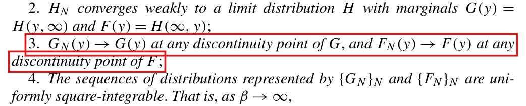
Condition 3 of Proposition 1 (p. 855). GN(y)→G(y)G_N(y)\to G(y) at any discontinuity point of GG, and FN(y)→F(y)F_N(y)\to F(y) at any discontinuity point of FF;

Remark 1 (p. 855). Condition 3 is used to establish the functional convergence of (GN,FN)(G_N,F_N) to (G,F)(G,F).

Lemma 2 (p. 860). Suppose conditions 1–3 of Proposition 1 hold. Then

sup⁡y∣G(y)−GN(y)∣→0andsup⁡y∣F(y)−FN(y)∣→0.\sup_y|G(y)-G_N(y)|\to 0 \quad\text{and}\quad \sup_y|F(y)-F_N(y)|\to 0 .

In addition, given η1,η0>0\eta_1,\eta_0>0, there exist two positive integers K1(η1)K_1(\eta_1) and K0(η0)K_0(\eta_0) such that

lim sup⁡N{N P(sup⁡y∣G(y)−G^N(y)∣≥η1)}≤(1−θρ)K1(η1)θρ η12,lim sup⁡N{N P(sup⁡y∣F(y)−F^N(y)∣≥η0)}≤{1−θ(1−ρ)}K0(η0)θ(1−ρ) η02.\begin{aligned} \limsup_N\Bigl\{N\,\mathrm{P}\Bigl(\sup_y|G(y)-\hat G_N(y)|\ge\eta_1\Bigr)\Bigr\} &\le \frac{(1-\theta\rho)K_1(\eta_1)}{\theta\rho\,\eta_1^2},\\ \limsup_N\Bigl\{N\,\mathrm{P}\Bigl(\sup_y|F(y)-\hat F_N(y)|\ge\eta_0\Bigr)\Bigr\} &\le \frac{\{1-\theta(1-\rho)\}K_0(\eta_0)}{\theta(1-\rho)\,\eta_0^2}. \end{aligned}

The integers are nonincreasing in η\eta, and depend also on the limiting distribution HH of (y1,y0)(y_1,y_0).

Proof of Lemma 2 (p. 861). hence sup⁡y∣G(y)−GN(y)∣<η1\sup_y|G(y)-G_N(y)|<\eta_1 if ∣G(si−1)−GN(si−1)∣<η1/2|G(s_{i-1})-G_N(s_{i-1})|<\eta_1/2 and ∣G(si−)−GN(si−)∣<η1/2|G(s_i-)-G_N(s_i-)|<\eta_1/2 for all ii. By conditions 2 and 3, this is satisfied for all NN sufficiently large.

The problem

Lemma 2 makes two assertions about the distribution functions GNG_N and FNF_N of the potential outcomes in the population UNU_N and their sample analogues G^N\hat G_N and F^N\hat F_N. The first is that GNG_N and FNF_N converge uniformly to their limits GG and FF. The second is that the probability of a uniform error of at least η\eta between a sample distribution function and its limit is at most of order 1/N1/N. Neither follows from conditions 1–3. Weak convergence (condition 2) implies that GN(y)→G(y)G_N(y)\to G(y) at the points where GG is continuous, and condition 3 adds the points where GG jumps. Uniform convergence also requires the left limits to converge at the jumps, that is, GN(y−)→G(y−)G_N(y-)\to G(y-), and no condition supplies this. The proof on p. 861 needs ∣G(si−)−GN(si−)∣<η1/2|G(s_i-)-G_N(s_i-)|<\eta_1/2 for large NN and obtains it “by conditions 2 and 3”. At a jump of GG this step can fail. If the outcomes of a population approach a jump point of GG from below without reaching it, then conditions 1–4 can hold while the uniform error stays at 1/21/2 or above for every NN and every assignment.

The lemma underlies Remark 1, the proof outline on p. 856, stages (i) and (ii) in the proof of Proposition 1 on p. 862, and the bounds for the last terms in the proof of Proposition 2 on pp. 867–869. Those steps are not justified by the stated conditions when GG or FF has a jump. The conclusions of Propositions 1 and 2 are not affected, since both hold under their printed hypotheses by arguments that do not pass through uniform convergence. To repair the lemma, one regularity condition must be added. That condition holds when GG and FF are continuous, and it holds with probability one when the units are independent and identically distributed draws from a superpopulation.

Evidence an exact counterexample

The evidence is an exact counterexample to the lemma, together with derivations of the corrected statements.

The counterexample. For i=1,2,…i=1,2,\ldots, let (ai,bi)(a_i,b_i) run through the cycle (0,0),(0,1),(1,0),(1,1)(0,0),(0,1),(1,0),(1,1), and define

y1i=ai−1i+2,y0i=bi−1i+2.y_{1i} = a_i - \frac{1}{i+2}, \qquad y_{0i} = b_i - \frac{1}{i+2}.

Let UNU_N consist of the first NN units, for N≥4N\ge 4, and set n=Nn=N and m=⌊N/2⌋m=\lfloor N/2\rfloor. The populations are nested and the outcomes are fixed. Condition 1 holds with θ=1\theta=1 and ρ=1/2\rho=1/2. Condition 2 holds: HNH_N converges weakly to the distribution HH with mass 1/41/4 at each of the points (0,0)(0,0), (0,1)(0,1), (1,0)(1,0) and (1,1)(1,1). Both marginals of HH have mass 1/21/2 at 00 and at 11, so that G(x)=F(x)=1/2G(x)=F(x)=1/2 for 0≤x<10\le x<1. Condition 3 holds as well. Since y1i≤0y_{1i}\le 0 exactly when ai=0a_i=0, I have GN(0)→1/2=G(0)G_N(0)\to 1/2 = G(0), and since every outcome is below 11, I have GN(1)=1=G(1)G_N(1)=1=G(1); the same holds for FNF_N. All outcomes lie in (−1,1)(-1,1), which implies condition 4, the boundedness assumed in Proposition 2 and the moment condition of Corollary 1. The distribution HH is not concentrated on a line.

Set tN=1−1/{2(N+2)}t_N = 1 - 1/\{2(N+2)\}. For i≤Ni\le N, I have y1i≤1−1/(N+2)<tNy_{1i}\le 1-1/(N+2) < t_N and y0i≤1−1/(N+2)<tNy_{0i}\le 1-1/(N+2) < t_N, and tN<1t_N<1. Then GN(tN)=FN(tN)=1G_N(t_N)=F_N(t_N)=1, and G^N(tN)=F^N(tN)=1\hat G_N(t_N)=\hat F_N(t_N)=1 for every assignment, while G(tN)=F(tN)=1/2G(t_N)=F(t_N)=1/2. This implies that, for every N≥4N\ge 4 and every assignment,

sup⁡y∣G(y)−GN(y)∣≥12,sup⁡y∣G(y)−G^N(y)∣≥12,\sup_y|G(y)-G_N(y)|\ge \frac12, \qquad \sup_y|G(y)-\hat G_N(y)|\ge\frac12,

and likewise for FF, FNF_N and F^N\hat F_N. The first assertion of the lemma fails. For η1=η0=1/4\eta_1=\eta_0=1/4, the two probabilities in the second assertion equal 11, and NN times each of them tends to infinity, while the right-hand sides equal 16K1(1/4)16K_1(1/4) and 16K0(1/4)16K_0(1/4). There exist no integers K1(1/4)K_1(1/4) and K0(1/4)K_0(1/4) for which the second assertion holds. Note that the left limits that the proof requires do not converge: GN(0−)→1/2G_N(0-)\to 1/2 while G(0−)=0G(0-)=0, and GN(1−)=1G_N(1-)=1 while G(1−)=1/2G(1-)=1/2. The table lists exact values at three population sizes, obtained by enumerating every assignment.

The counterexample at three population sizes, with η1=1/4\eta_1=1/4 and m=N/2m=N/2. The population error is sup⁡y∣G(y)−GN(y)∣\sup_y|G(y)-G_N(y)|. The smallest sample error is the minimum of sup⁡y∣G(y)−G^N(y)∣\sup_y|G(y)-\hat G_N(y)| over all assignments, and the probability is that of the event sup⁡y∣G(y)−G^N(y)∣≥1/4\sup_y|G(y)-\hat G_N(y)|\ge 1/4 over all assignments. Every entry is exact, and the same values hold for FF, FNF_N and F^N\hat F_N.
NNAssignmentsPopulation errorSmallest sample errorProbability
461/21/21/21/21
8701/21/21/21/21
129241/21/21/21/21

The added condition suffices. I write PP for GG or FF, PNP_N for the corresponding distribution function in the population, and P^N\hat P_N for the one in the sample, with kk sampled units and α=lim⁡k/N>0\alpha=\lim k/N>0. By weak convergence, I have PN(x)→P(x)P_N(x)\to P(x) and PN(x−)→P(x−)P_N(x-)\to P(x-) at every continuity point xx of PP. At the discontinuity points, both limits hold by condition 3 and the added condition. Fix η\eta such that 0<η≤10<\eta\le 1, and set R=⌈4/η⌉R=\lceil 4/\eta\rceil. The points ±∞\pm\infty and the distinct quantiles of PP at the levels j/Rj/R, for 1≤j≤R−11\le j\le R-1, form a partition with at most RR intervals such that P(t−)−P(s)≤1/RP(t-)-P(s)\le 1/R for adjacent points s<ts<t. Since distribution functions are monotone, for every distribution function AA, I have

sup⁡x∣P(x)−A(x)∣≤1R+max⁡{∣P(s)−A(s)∣, ∣P(t−)−A(t−)∣},\sup_x|P(x)-A(x)| \le \frac1R + \max\bigl\{|P(s)-A(s)|,\ |P(t-)-A(t-)|\bigr\},

where the maximum is over the adjacent points s<ts<t of the partition. Taking A=PNA=P_N, I obtain the uniform convergence. For A=P^NA=\hat P_N, each of the at most 2R2R values P^N(s)\hat P_N(s) and P^N(t−)\hat P_N(t-) has mean PN(s)P_N(s) or PN(t−)P_N(t-) and variance at most (N−k)/{4(N−1)k}(N-k)/\{4(N-1)k\}. Using Chebyshev’s inequality and the union bound, I obtain

lim sup⁡NN P(sup⁡x∣P(x)−P^N(x)∣≥η)≤2R(1−α)αη2.\limsup_N N\,\mathrm{P}\Bigl(\sup_x|P(x)-\hat P_N(x)|\ge\eta\Bigr) \le \frac{2R(1-\alpha)}{\alpha\eta^2}.

This is the printed bound with K(η)=2⌈4/η⌉K(\eta)=2\lceil 4/\eta\rceil. For η>1\eta>1 the event is empty.

Proposition 1 without the lemma. Let c>0c>0 be such that m≥cNm\ge cN and n−m≥cNn-m\ge cN for all large NN. For fixed xx, the value G^N(x)\hat G_N(x) has mean GN(x)G_N(x) and variance at most 1/(4cN)1/(4cN), so that G^N(x)−GN(x)→0\hat G_N(x)-G_N(x)\to 0 in probability. By condition 2, G^N\hat G_N converges weakly to GG in probability, and the same holds for F^N\hat F_N and FF. For every sample and every T>0T>0, I have

∫x2 1{∣x∣>T} dG^N(x)≤Nm∫x2 1{∣x∣>T} dGN(x),\int x^2\,\mathbf{1}\{|x|>T\}\,d\hat G_N(x) \le \frac{N}{m}\int x^2\,\mathbf{1}\{|x|>T\}\,dG_N(x),

and by condition 4 the sampled distributions are uniformly square-integrable. Weak convergence and uniform square-integrability imply that the quantile functions converge in L2(0,1)L^2(0,1), in probability for the samples. The means, the second moments and the two integrals of products of quantile functions in (7)–(9) are continuous in the quantile functions with respect to that norm. I conclude that NVNHNV_N^H and NVNLNV_N^L have the limits stated in Proposition 1, and that N(V^NB−VNB)→0N(\hat V_N^B-V_N^B)\to 0 in probability for B∈{H,L}B\in\{H,L\}. Condition 3 is not used.

Proposition 2 without the lemma. Suppose ∣y1i∣≤C|y_{1i}|\le C and ∣y0i∣≤C|y_{0i}|\le C, and write P1N=GNP_{1N}=G_N, P0N=FNP_{0N}=F_N, k1=mk_1=m and k0=n−mk_0=n-m. For a∈{0,1}a\in\{0,1\}, define

Da=∫−CC∣P^aN(x)−PaN(x)∣ dx.D_a=\int_{-C}^{C}|\hat P_{aN}(x)-P_{aN}(x)|\,dx .

By the Cauchy–Schwarz inequality and the bound on the variance above, I have E Da2≤C2/(cN)\mathrm{E}\,D_a^2\le C^2/(cN), so that E(D1+D0)2≤4C2/(cN)\mathrm{E}(D_1+D_0)^2\le 4C^2/(cN). The quantile functions qAq_A and qPq_P of two distributions on [−C,C][-C,C] with distribution functions AA and PP satisfy ∫01∣qA(u)−qP(u)∣ du=∫−CC∣A(x)−P(x)∣ dx\int_0^1|q_A(u)-q_P(u)|\,du=\int_{-C}^{C}|A(x)-P(x)|\,dx. It follows that the error of the sample mean in arm aa is at most DaD_a, the error of the unbiased variance estimator is at most 8CDa+C2/(ka−1)8CD_a+C^2/(k_a-1), and the error of each estimated covariance bound in (8) is at most 2C(D1+D0)2C(D_1+D_0). Substituting these bounds into (9), I obtain, for N≥2/cN\ge 2/c and B∈{H,L}B\in\{H,L\},

N∣V^NB−VNB∣≤(16c+8)C(D1+D0)+8C2c2N.N|\hat V_N^B-V_N^B| \le \Bigl(\frac{16}{c}+8\Bigr)C(D_1+D_0)+\frac{8C^2}{c^2N}.

Markov’s inequality then implies the bound stated in the correction below.

What survives

Lemma 1 and the sharpness of the interval [VNL,VNH][V_N^L,V_N^H], the bounds and estimators (7)–(9), and the ordering of V^NH\hat V_N^H and V^NL\hat V_N^L relative to Neyman’s bounds do not depend on Lemma 2. Propositions 1 and 2 keep their hypotheses and conclusions. With them stand the consistency of V^NH\hat V_N^H used in Corollary 1 and the argument for asymptotically conservative Wald intervals. This error does not change the computations in the application, the simulations or Appendix C. Three things change: Lemma 2 gains a hypothesis, Remark 1 is reworded, and the proof outline and the steps in the proofs of Propositions 1 and 2 that rest on the lemma are replaced.

Corrected

Lemma 2. Suppose conditions 1–3 of Proposition 1 hold, that is, (m/N,n/N)→(θρ,θ)(m/N,n/N)\to(\theta\rho,\theta) for θ∈(0,1]\theta\in(0,1] and ρ∈(0,1)\rho\in(0,1); HNH_N converges weakly to a limit distribution HH with marginals G(y)=H(y,∞)G(y)=H(y,\infty) and F(y)=H(∞,y)F(y)=H(\infty,y); and GN(y)→G(y)G_N(y)\to G(y) at any discontinuity point of GG, and FN(y)→F(y)F_N(y)\to F(y) at any discontinuity point of FF. Suppose in addition that GN(y−)→G(y−)\colorbox{#ffe58a}{$G_N(y-)\to G(y-)$} at any discontinuity point of GG, and FN(y−)→F(y−)\colorbox{#ffe58a}{$F_N(y-)\to F(y-)$} at any discontinuity point of FF. Then

sup⁡y∣G(y)−GN(y)∣→0andsup⁡y∣F(y)−FN(y)∣→0.\sup_y|G(y)-G_N(y)|\to 0 \quad\text{and}\quad \sup_y|F(y)-F_N(y)|\to 0 .

In addition, given η1,η0>0\eta_1,\eta_0>0, there exist two positive integers K1(η1)K_1(\eta_1) and K0(η0)K_0(\eta_0) such that

lim sup⁡N{N P(sup⁡y∣G(y)−G^N(y)∣≥η1)}≤(1−θρ)K1(η1)θρ η12,lim sup⁡N{N P(sup⁡y∣F(y)−F^N(y)∣≥η0)}≤{1−θ(1−ρ)}K0(η0)θ(1−ρ) η02.\begin{aligned} \limsup_N\Bigl\{N\,\mathrm{P}\Bigl(\sup_y|G(y)-\hat G_N(y)|\ge\eta_1\Bigr)\Bigr\} &\le \frac{(1-\theta\rho)K_1(\eta_1)}{\theta\rho\,\eta_1^2},\\ \limsup_N\Bigl\{N\,\mathrm{P}\Bigl(\sup_y|F(y)-\hat F_N(y)|\ge\eta_0\Bigr)\Bigr\} &\le \frac{\{1-\theta(1-\rho)\}K_0(\eta_0)}{\theta(1-\rho)\,\eta_0^2}. \end{aligned}

The integers are nonincreasing in η\eta, and K1(η)=K0(η)=2⌈4/min⁡(η,1)⌉K_1(\eta)=K_0(\eta)=2\lceil 4/\min(\eta,1)\rceil is an admissible choice.

Remark 1. Condition 3, together with the convergence of the left limits GN(y−)→G(y−)G_N(y-)\to G(y-) and FN(y−)→F(y−)F_N(y-)\to F(y-) at the same points, is used to establish the functional convergence of (GN,FN)(G_N,F_N) to (G,F)(G,F). When the units of UNU_N are independent and identically distributed samples from a superpopulation, both conditions hold with probability one, and both are satisfied if GG and FF are continuous.

Proposition 1. The statement is unchanged. The proof outline and stages (i) and (ii) of the proof rest on the uniform convergence of (G^N,F^N)(\hat G_N,\hat F_N) to (G,F)(G,F). They are replaced by the weak convergence of G^N\hat G_N and F^N\hat F_N to GG and FF in probability and, by condition 4, the convergence of their quantile functions in L2(0,1)L^2(0,1) in probability. No condition at the discontinuity points is needed.

Proposition 2. The statement is unchanged. The steps of the proof that apply Lemma 2 are replaced by the following bound. Suppose ∣y1i∣≤C|y_{1i}|\le C and ∣y0i∣≤C|y_{0i}|\le C for all ii, and let c>0c>0 be such that m≥cNm\ge cN and n−m≥cNn-m\ge cN for all large NN, as condition 1 allows. Then for B∈{H,L}B\in\{H,L\}, every ε>0\varepsilon>0, and every such NN with N≥max⁡{2/c, 16C2/(c2ε)}N\ge\max\{2/c,\ 16C^2/(c^2\varepsilon)\},

P{N∣V^NB−VNB∣≥ε}≤16 (16/c+8)2 C4cNε2.\mathrm{P}\bigl\{N|\hat V_N^B-V_N^B|\ge\varepsilon\bigr\} \le \frac{16\,(16/c+8)^2\,C^4}{cN\varepsilon^2}.
The opening of Lemma 2. A red box marks the words 'Suppose conditions 1-3 of Proposition 1 hold. Then'. The display below it states that the supremum over y of the distance between G and G N tends to 0, and likewise for F and F N.
Lemma 2, p. 860 (PDF p. 11): the hypothesis and the first assertion. The marked line states the hypothesis, conditions 1–3 of Proposition 1.
Four lines from the proof of Lemma 2. A red box marks the sentence 'By conditions 2 and 3, this is satisfied for all N sufficiently large', which follows the requirement that the distance between G and G N at the points s i minus 1, and between their left limits at s i, be below eta 1 over 2.
Proof of Lemma 2, p. 861 (PDF p. 12). The marked sentence obtains the convergence of the left limits GN(si−)G_N(s_i-) from conditions 2 and 3.
Conditions 2, 3 and 4 of Proposition 1. A red box marks condition 3: 'G N of y tends to G of y at any discontinuity point of G, and F N of y tends to F of y at any discontinuity point of F'.
Proposition 1, p. 855 (PDF p. 6). The marked condition 3 concerns the values GN(y)G_N(y) and FN(y)F_N(y) at the discontinuity points of GG and FF, and not the left limits.
The first three lines of Remark 1. A red box marks the sentence 'Condition 3 is used to establish the functional convergence of (G N, F N) to (G, F)'.
Remark 1, p. 855 (PDF p. 6). The marked sentence says what condition 3 is used for.
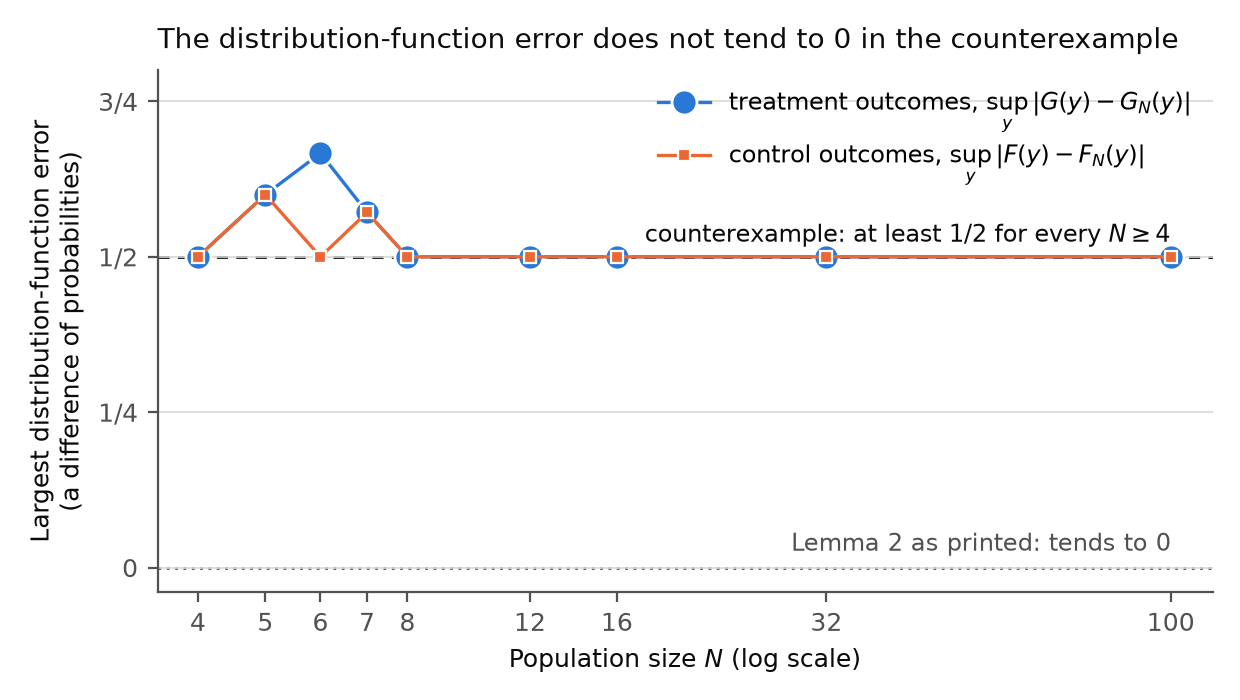
Line chart with population size N from 4 to 100 on a logarithmic horizontal axis and the largest distribution-function error on the vertical axis, with tick labels from 0 to 3/4. Treatment outcomes (blue circles) and control outcomes (orange squares) both take the values 1/2, 3/5 and 4/7 at N equal to 4, 5 and 7. At N equal to 6, the treatment error is 2/3 and the control error is 1/2. Both series equal 1/2 at N equal to 8, 12, 16, 32 and 100. A dashed line at 1/2 is labelled 'counterexample: at least 1/2 for every N at least 4', and a dotted line at 0 is labelled 'Lemma 2 as printed: tends to 0'.
The counterexample to Lemma 2. The largest error of the population distribution functions, sup⁡y∣G(y)−GN(y)∣\sup_y|G(y)-G_N(y)| and sup⁡y∣F(y)−FN(y)∣\sup_y|F(y)-F_N(y)|, is shown at nine population sizes from 4 to 100 (exact values). It is never below 1/21/2, where Lemma 2 as printed asserts convergence to 0.

Minor (8)

Real but inconsequential, for example a misprint that does not change a result.

The last relation in equation (11) is an upper bound, not an equality.

Proof of Lemma 2, equation (11), p. 861 (PDF p. 12)

See also under Formal statements (Lean): P022-T4, P022-T5

As printed

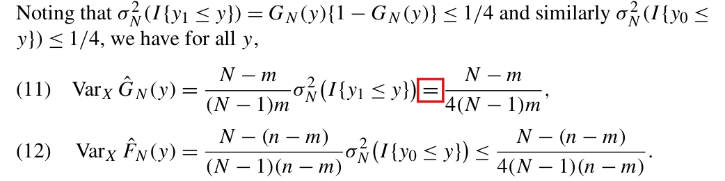
Noting that σN2(I{y1≤y})=GN(y){1−GN(y)}≤1/4\sigma_N^2(I\{y_1\le y\})=G_N(y)\{1-G_N(y)\}\le 1/4 and similarly σN2(I{y0≤y})≤1/4\sigma_N^2(I\{y_0\le y\})\le 1/4, we have for all yy,

Var⁡XG^N(y)=N−m(N−1)m σN2(I{y1≤y}) = N−m4(N−1)m,(11)\operatorname{Var}_X\hat G_N(y)=\frac{N-m}{(N-1)m}\,\sigma_N^2\bigl(I\{y_1\le y\}\bigr)\ \colorbox{#ffe58a}{$\displaystyle =$}\ \frac{N-m}{4(N-1)m}, \qquad (11)
The problem

The variance σN2(I{y1≤y})=GN(y){1−GN(y)}\sigma_N^2(I\{y_1\le y\})=G_N(y)\{1-G_N(y)\} is at most 1/41/4, and it equals 1/41/4 only when GN(y)=1/2G_N(y)=1/2. The last relation in (11) is therefore an inequality. The sentence before the display and the companion display (12) state the bound correctly.

Evidence an exact counterexample

I used an exact counterexample. Let N=4N=4 and m=2m=2, and take yy below every potential outcome under treatment. Then G^N(y)=0\hat G_N(y)=0 in each of the six assignments, so that Var⁡XG^N(y)=0\operatorname{Var}_X\hat G_N(y)=0, while the right-hand side of (11) is (4−2)/(4⋅3⋅2)=1/12(4-2)/(4\cdot 3\cdot 2)=1/12.

What survives

The proof substitutes (11) into (10), and that step uses only the upper bound. The bound that follows is unchanged. The separate problem with Lemma 2 is P022-E001.

Corrected

Let GNG_N be the distribution function of y1y_1 in the population UNU_N, and let G^N\hat G_N be the distribution function of the observed outcomes of the mm units assigned to treatment. For all yy,

Var⁡XG^N(y)=N−m(N−1)m GN(y){1−GN(y)} ≤ N−m4(N−1)m.(11)\operatorname{Var}_X\hat G_N(y)=\frac{N-m}{(N-1)m}\,G_N(y)\{1-G_N(y)\}\ \colorbox{#ffe58a}{$\displaystyle \le$}\ \frac{N-m}{4(N-1)m}. \qquad (11)
Equations (11) and (12) with the sentence that introduces them. A red box marks the second equals sign in equation (11), between the term with sigma squared N and the fraction N minus m over 4 (N minus 1) m. In equation (12) the corresponding sign is 'less than or equal to'.
Proof of Lemma 2, equations (11) and (12), p. 861 (PDF p. 12). The marked sign in (11) is printed as an equality; the corresponding sign in (12) is an inequality.

In the proof of the first bound of Proposition 2, the last term must receive a positive share of the tolerance ε1\varepsilon_1, such as ε1/2\varepsilon_1/2, in place of 1−ε11-\varepsilon_1, and the concluding display concerns VNHV_N^H, not VNV_N.

Proof of Proposition 2, bound for the last term, p. 867 (PDF p. 18), through equation (23) and the display after it, p. 868 (PDF p. 19)

See also under Formal statements (Lean): P022-T6, P022-T7

As printed

p. 865. Let ν1,…,ν8>0\nu_1,\ldots,\nu_8>0 be a tuple whose sum is ε1\colorbox{#ffe58a}{$\varepsilon_1$}.

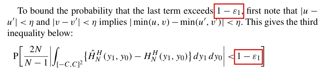
p. 867. To bound the probability that the last term exceeds 1−ε1\colorbox{#ffe58a}{$1-\varepsilon_1$}, first note that ∣u−u′∣<η|u-u'|<\eta and ∣v−v′∣<η|v-v'|<\eta implies ∣min⁡(u,v)−min⁡(u′,v′)∣<η|\min(u,v)-\min(u',v')|<\eta. This gives the third inequality below:

P[2NN−1∣∫[−C,C]2{H^NH(y1,y0)−HNH(y1,y0)} dy1 dy0∣<1−ε1]≥P{sup⁡y1,y0∣H^NH(y1,y0)−HNH(y1,y0)∣<(N−1)(1−ε1)8NC2}\begin{aligned} &\mathrm{P}\Bigl[\frac{2N}{N-1}\Bigl|\int_{[-C,C]^2}\bigl\{\hat H_N^H(y_1,y_0)-H_N^H(y_1,y_0)\bigr\}\,dy_1\,dy_0\Bigr|<\colorbox{#ffe58a}{$\displaystyle 1-\varepsilon_1$}\Bigr]\\ &\qquad\ge \mathrm{P}\Bigl\{\sup_{y_1,y_0}\bigl|\hat H_N^H(y_1,y_0)-H_N^H(y_1,y_0)\bigr|<\frac{(N-1)(\colorbox{#ffe58a}{$\displaystyle 1-\varepsilon_1$})}{8NC^2}\Bigr\} \end{aligned}

p. 868, equation (23) and the text after it.

lim sup⁡NN P[2NN−1∣∫[−C,C]2{H^NH(y1,y0)−HNH(y1,y0)} dy1 dy0∣≥1−ε1]≤C4κ1(ε1).\limsup_N N\,\mathrm{P}\Bigl[\frac{2N}{N-1}\Bigl|\int_{[-C,C]^2}\bigl\{\hat H_N^H(y_1,y_0)-H_N^H(y_1,y_0)\bigr\}\,dy_1\,dy_0\Bigr|\ge\colorbox{#ffe58a}{$\displaystyle 1-\varepsilon_1$}\Bigr]\le C^4\kappa_1(\varepsilon_1).

The bounds (17)–(23) imply that

lim sup⁡NN P(N∣V^NH−VN∣≥ε)≤C4(∑i=18ciνi2+κ1(ε1)).\limsup_N N\,\mathrm{P}\bigl(N|\hat V_N^H-\colorbox{#ffe58a}{$\displaystyle V_N$}|\ge\varepsilon\bigr)\le C^4\Bigl(\sum_{i=1}^8\frac{c_i}{\nu_i^2}+\kappa_1(\varepsilon_1)\Bigr).

By minimizing the right-hand side over ν1,…,ν8>0\nu_1,\ldots,\nu_8>0 subject to the constraint ν1+⋯+ν8=ε1\nu_1+\cdots+\nu_8=\colorbox{#ffe58a}{$\varepsilon_1$}, the sum in the parenthesis can be absorbed into κ1(ε1)\kappa_1(\varepsilon_1), yielding the desired convergence rate for NV^NHN\hat V_N^H.

The problem

Proposition 2 bounds P{N∣V^NH−VNH∣≥ε}\mathrm{P}\{N|\hat V_N^H-V_N^H|\ge\varepsilon\} for an arbitrary ε>0\varepsilon>0, with ε1+ε2+ε3=ε\varepsilon_1+\varepsilon_2+\varepsilon_3=\varepsilon. The proof splits N(V^NH−VNH)N(\hat V_N^H-V_N^H) into seven terms. The first six receive the tolerances ν1,…,ν8\nu_1,\ldots,\nu_8, whose sum is ε1\varepsilon_1, and the last receives 1−ε11-\varepsilon_1. The tolerances add to 11 and not to ε\varepsilon. As printed, the argument bounds the event {N∣V^NH−VNH∣≥1}\{N|\hat V_N^H-V_N^H|\ge 1\}. When ε1≥1\varepsilon_1\ge 1 the tolerance 1−ε11-\varepsilon_1 is not positive, and (23) cannot hold with a finite κ1(ε1)\kappa_1(\varepsilon_1). The display after (23) has a second slip: it names the true variance VNV_N where the sharp upper bound VNHV_N^H is meant. Read literally, it says that NV^NHN\hat V_N^H concentrates around NVNNV_N, which is false when the bound is not attained.

Evidence a derivation

The evidence is a derivation with two exact examples. For the tolerance, take ε=3\varepsilon=3 and ε1=ε2=ε3=1\varepsilon_1=\varepsilon_2=\varepsilon_3=1. The event in (23) is then that a nonnegative quantity is at least 00. It has probability 11, and the left-hand side of (23) is infinite. For the target, let N=n=4rN=n=4r and m=N/2m=N/2, with rr units at each of the points (0,0)(0,0), (0,1)(0,1), (1,0)(1,0) and (1,1)(1,1). Both marginal variances are 1/41/4, the covariance is 00 and its sharp upper bound is 1/41/4, so that NVN=N/{2(N−1)}NV_N=N/\{2(N-1)\} and NVNH=N/(N−1)NV_N^H=N/(N-1). Since NV^NH→1N\hat V_N^H\to 1 in probability, N∣V^NH−VN∣N|\hat V_N^H-V_N| tends to 1/21/2 and not to 00.

The repair rests on the inequality that the proof already uses. Since the square [−C,C]2[-C,C]^2 has area 4C24C^2, I have

2NN−1∣∫[−C,C]2{H^NH(y1,y0)−HNH(y1,y0)} dy1 dy0∣≤8NC2N−1sup⁡y1,y0∣H^NH(y1,y0)−HNH(y1,y0)∣.\frac{2N}{N-1}\Bigl|\int_{[-C,C]^2}\bigl\{\hat H_N^H(y_1,y_0)-H_N^H(y_1,y_0)\bigr\}\,dy_1\,dy_0\Bigr|\le\frac{8NC^2}{N-1}\sup_{y_1,y_0}\bigl|\hat H_N^H(y_1,y_0)-H_N^H(y_1,y_0)\bigr| .

A tolerance x>0x>0 for the last term therefore corresponds to the threshold (N−1)x/(8NC2)(N-1)x/(8NC^2) for the supremum. With x=ε1/2x=\varepsilon_1/2 and ν1+⋯+ν8=ε1/2\nu_1+\cdots+\nu_8=\varepsilon_1/2, the union bound controls the event {N∣V^NH−VNH∣≥ε1}\{N|\hat V_N^H-V_N^H|\ge\varepsilon_1\}, which contains the event at ε\varepsilon because ε1<ε\varepsilon_1<\varepsilon.

What survives

The statement of Proposition 2 and its O(1/N)O(1/N) rate are unaffected. The decomposition into seven terms and the bounds (17)–(22) stand, and the argument for V^NL\hat V_N^L keeps its own tolerance ε2+ε3\varepsilon_2+\varepsilon_3. The use of Lemma 2 in the same passage is a separate matter, treated in P022-E001, where the rate is obtained from a bound that does not use the lemma.

Corrected

p. 865, for the bound on V^NH\hat V_N^H. Let ν1,…,ν8>0\nu_1,\ldots,\nu_8>0 be a tuple whose sum is ε1/2\colorbox{#ffe58a}{$\varepsilon_1/2$}.

pp. 867–868. To bound the probability that the last term exceeds ε1/2\colorbox{#ffe58a}{$\varepsilon_1/2$}, replace 1−ε11-\varepsilon_1 by ε1/2\varepsilon_1/2 in every line of the two displays that follow, with 0<ξ<ε1/(16C2)0<\xi<\varepsilon_1/(16C^2) for C>0C>0 (the case C=0C=0 is trivial). Equation (23) becomes

lim sup⁡NN P[2NN−1∣∫[−C,C]2{H^NH(y1,y0)−HNH(y1,y0)} dy1 dy0∣≥ε1/2]≤C4κ1(ε1).\limsup_N N\,\mathrm{P}\Bigl[\frac{2N}{N-1}\Bigl|\int_{[-C,C]^2}\bigl\{\hat H_N^H(y_1,y_0)-H_N^H(y_1,y_0)\bigr\}\,dy_1\,dy_0\Bigr|\ge\colorbox{#ffe58a}{$\displaystyle \varepsilon_1/2$}\Bigr]\le C^4\kappa_1(\varepsilon_1).

The bounds (17)–(23) imply that

lim sup⁡NN P(N∣V^NH−VNH∣≥ε)≤C4(∑i=18ciνi2+κ1(ε1)).\limsup_N N\,\mathrm{P}\bigl(N|\hat V_N^H-\colorbox{#ffe58a}{$\displaystyle V_N^H$}|\ge\varepsilon\bigr)\le C^4\Bigl(\sum_{i=1}^8\frac{c_i}{\nu_i^2}+\kappa_1(\varepsilon_1)\Bigr).

By minimizing the right-hand side over ν1,…,ν8>0\nu_1,\ldots,\nu_8>0 subject to the constraint ν1+⋯+ν8=ε1/2\nu_1+\cdots+\nu_8=\colorbox{#ffe58a}{$\varepsilon_1/2$}, the sum in the parenthesis can be absorbed into κ1(ε1)\kappa_1(\varepsilon_1).

In the argument for V^NL\hat V_N^L the tuple keeps the sum ε1\varepsilon_1, as printed, and the last term keeps the tolerance ε2+ε3\varepsilon_2+\varepsilon_3.

Three lines of text and the first line of a display from the proof of Proposition 2. Red boxes mark '1 minus epsilon 1' twice: in the sentence 'To bound the probability that the last term exceeds 1 minus epsilon 1', and at the right end of the display, where the probability concerns an integral being less than 1 minus epsilon 1.
Proof of Proposition 2, p. 867 (PDF p. 18). The marked tolerance 1−ε11-\varepsilon_1 is assigned to the last term, in the sentence and in the first line of the display that follows.
The sentence 'The bounds (17)-(23) imply that' and the display below it. A red box marks the symbol V with subscript N, without a superscript, inside the absolute value 'V hat H N minus V N'.
Proof of Proposition 2, display after equation (23), p. 868 (PDF p. 19). The marked symbol is printed VNV_N, without the superscript HH.

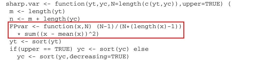
The multiplication sign that opens the second line of the definition of FPvar belongs at the end of the first line; as printed, the code does not parse.

Appendix B, R code of sharp.var, fourth and fifth printed lines, p. 869 (PDF p. 20)

As printed

Appendix B, p. 869, fourth and fifth lines of the function.

FPvar <- function(x,N) (N-1)/(N*(length(x)-1))\texttt{FPvar <- function(x,N) (N-1)/(N*(length(x)-1))}

  * sum((x - mean(x))^2)\texttt{~~}\colorbox{#ffe58a}{$\texttt{*}$}\texttt{~sum((x - mean(x))\textasciicircum 2)}

The problem

R ends a statement at a line break when the expression read so far is complete. The first of the two lines is a complete function definition. The second then begins a new statement with a binary operator, and the parser stops with the message unexpected '*' at line 5, column 5 of the function.

Evidence a recalculation from the source

I checked the code by running it. The block copied with its printed line breaks fails to parse at the place stated. With the operator moved to the end of the preceding line and no other change, the function parses and runs.

What survives

The formula intended for FPvar and the estimator are unchanged by the syntax repair. The reported numbers were not recomputed. Two further defects of the same function are P022-E002 and P022-E003.

Corrected

Fourth and fifth lines of the function.

FPvar <- function(x,N) (N-1)/(N*(length(x)-1)) *\texttt{FPvar <- function(x,N) (N-1)/(N*(length(x)-1))~}\colorbox{#ffe58a}{$\texttt{*}$}

  sum((x - mean(x))^2)\texttt{~~sum((x - mean(x))\textasciicircum 2)}

The first eight lines of the R function sharp.var. A red box marks the two lines 'FPvar <- function(x,N) (N-1)/(N*(length(x)-1))' and '* sum((x - mean(x))^2)'.
Appendix B, R code, p. 869 (PDF p. 20). The two marked lines define FPvar; the second begins with the multiplication sign.

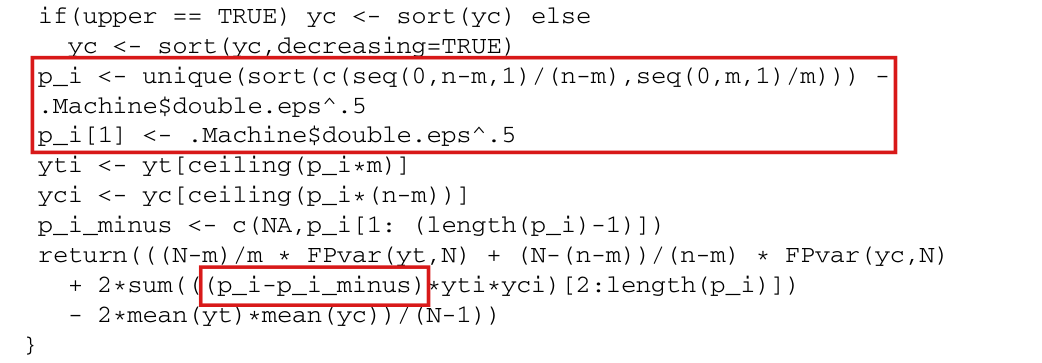
The printed function shifts the partition points by 2−262^{-26} and uses the shifted points as integration weights, which sum to 1−2−251-2^{-25}, and its output is not the estimate of equations (8)–(9); the widths pi−pi−1p_i-p_{i-1} must be kept, with the quantiles selected at the midpoints of the cells.

Appendix B, R code of sharp.var, p. 869 (PDF p. 20): the lines that set p_i and the weights in the return expression; equation (8), p. 854 (PDF p. 5)

See also under Formal statements (Lean): P022-T8, P022-T9

As printed

Appendix B, p. 869, ninth to seventeenth lines of the function.

p_i <- unique(sort(c(seq(0,n-m,1)/(n-m),seq(0,m,1)/m))) -\texttt{p\_i <- unique(sort(c(seq(0,n-m,1)/(n-m),seq(0,m,1)/m)))~}\colorbox{#ffe58a}{$\texttt{-}$}

.Machine$double.eps^.5\colorbox{#ffe58a}{$\texttt{.Machine\$double.eps\textasciicircum.5}$}

p_i[1] <- .Machine$double.eps^.5\colorbox{#ffe58a}{$\texttt{p\_i[1] <- .Machine\$double.eps\textasciicircum.5}$}

yti <- yt[ceiling(p_i*m)]\texttt{yti <- yt[ceiling(p\_i*m)]}

yci <- yc[ceiling(p_i*(n-m))]\texttt{yci <- yc[ceiling(p\_i*(n-m))]}

p_i_minus <- c(NA,p_i[1: (length(p_i)-1)])\texttt{p\_i\_minus <- c(NA,p\_i[1: (length(p\_i)-1)])}

return(((N-m)/m * FPvar(yt,N) + (N-(n-m))/(n-m) * FPvar(yc,N)\texttt{return(((N-m)/m * FPvar(yt,N) + (N-(n-m))/(n-m) * FPvar(yc,N)}

  + 2*sum(((p_i-p_i_minus)*yti*yci)[2:length(p_i)])\texttt{~~+ 2*sum((}\colorbox{#ffe58a}{$\texttt{(p\_i-p\_i\_minus)}$}\texttt{*yti*yci)[2:length(p\_i)])}

  - 2*mean(yt)*mean(yc))/(N-1))\texttt{~~- 2*mean(yt)*mean(yc))/(N-1))}

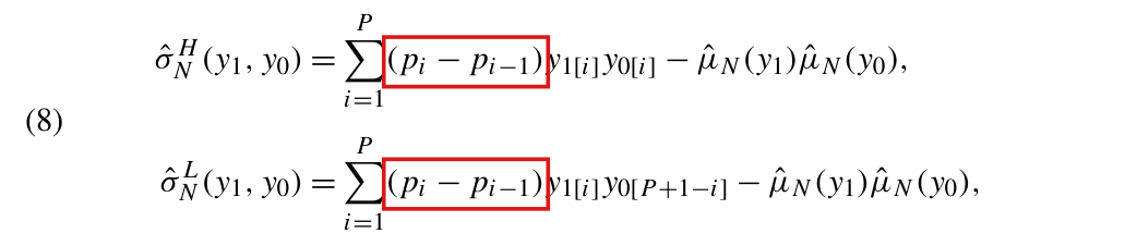
Equation (8), p. 854.

σ^NH(y1,y0)=∑i=1P(pi−pi−1) y1[i]y0[i]−μ^N(y1)μ^N(y0),σ^NL(y1,y0)=∑i=1P(pi−pi−1) y1[i]y0[P+1−i]−μ^N(y1)μ^N(y0),\begin{aligned} \hat\sigma_N^H(y_1,y_0)&=\sum_{i=1}^P(p_i-p_{i-1})\,y_{1[i]}y_{0[i]}-\hat\mu_N(y_1)\hat\mu_N(y_0),\\ \hat\sigma_N^L(y_1,y_0)&=\sum_{i=1}^P(p_i-p_{i-1})\,y_{1[i]}y_{0[P+1-i]}-\hat\mu_N(y_1)\hat\mu_N(y_0), \end{aligned}
The problem

Equation (8) weights each product of order statistics by the width pi−pi−1p_i-p_{i-1} of a cell of the partition Pm,nP_{m,n} of [0,1][0,1], and the widths sum to 11. The function subtracts e=.Machine$double.eps=2−26e=\sqrt{\texttt{.Machine\$double.eps}}=2^{-26} from every partition point, resets the first point to ee, and uses the shifted points both to select the order statistics and as weights. When every cell is wider than 2e2e, the shifted points select the order statistics of (8). The first weight, however, becomes p1−p0−2ep_1-p_0-2e, and the weights sum to 1−2e=1−2−251-2e=1-2^{-25}. A fraction 2e2e of the first product is lost from the sum. The output is then not invariant to adding a constant to every outcome, as the estimate (9) is, and it can be negative. The discrepancy is about 6×10−86\times10^{-8} times the product of two extreme outcomes, divided by N−1N-1. For the application, with N=1561N=1561 and outcomes between $0 and $150, it is at most 8.6×10−78.6\times10^{-7} USD2^2, against a reported estimate of 0.186. It vanishes for the upper bound when the smallest outcome in either arm is zero.

Evidence an exact counterexample

I checked an exact counterexample in rational arithmetic and reproduced it in R. Let k=n−mk=n-m, and suppose every cell of the partition is wider than 2e2e, so that the shifted points select the same order statistics as (8). Let a1a_1 be the smallest outcome under treatment, and let b∗b_* be the smallest outcome under control for the upper bound and the largest for the lower bound. Since only the first weight changes, the output of the printed function differs from the estimate (9) by exactly

−4e a1b∗N−1,e=2−26.-\frac{4e\,a_1b_*}{N-1}, \qquad e=2^{-26}.

With all outcomes equal to 11, N=n=4N=n=4 and m=2m=2, the randomization variance and both estimates (9) are 00, and the printed function returns −4e/3=−1/50331648-4e/3=-1/50331648 for both bounds; R returns −1.9868×10⁻⁸-1.9868\times10^{-8}. The table lists this case and three others.

The estimate of equation (9) and the output of the printed function, in exact arithmetic with e=2−26e=2^{-26}. The line break in the definition of FPvar is joined.
Outcomes in the two armsNNBoundEquation (9)Printed function
(1,1)(1,1) in both4upper00−1/50331648≈−1.99×10−8-1/50331648\approx-1.99\times10^{-8}
(1,1)(1,1) in both4lower00−1/50331648≈−1.99×10−8-1/50331648\approx-1.99\times10^{-8}
(0,1)(0,1) in both4upper5/125/125/125/12
(0,1)(0,1) in both4lower1/121/121/121/12
(106,106+1)(10^6,10^6+1) in both4upper5/125/12−244135505/12288≈−19867.80-244135505/12288\approx-19867.80
(106,106+1)(10^6,10^6+1) in both4lower1/121/12−15624950089/786432≈−19868.15-15624950089/786432\approx-19868.15
treatment (−2,1,4)(-2,1,4), control (1,3)(1,3)8upper179/56179/56179/56+1/58720256179/56+1/58720256
treatment (−2,1,4)(-2,1,4), control (1,3)(1,3)8lower115/56115/56115/56+3/58720256115/56+3/58720256

The third and fourth rows agree because a1=0a_1=0. The fifth and sixth rows are the third and fourth with 10610^6 added to every outcome, which leaves (9) unchanged. For the application, the cells of the partition have width at least 1/(781⋅780)>2e1/(781\cdot780)>2e, and by the displayed formula the discrepancy is at most 4e⋅1502/1560=375/436207616≈8.6×10−74e\cdot150^2/1560=375/436207616\approx8.6\times10^{-7} USD2^2. Since the data are not available, no entry of Table 1 or Table 2 was recomputed, and none is shown to change.

What survives

The definitions (7)–(9), the sharpness of the bounds and the asymptotic results concern the estimators as defined in the text and are unaffected. Table 3 was computed by numerical integration of Beta quantile functions and does not use this function. No number in Table 1 or Table 2 is shown to be wrong.

Corrected

Keep the partition 0=p0<p1<⋯<pP=10=p_0<p_1<\cdots<p_P=1 of equation (8) and its widths, and select the order statistics at the midpoints ur=(pr−1+pr)/2u_r=(p_{r-1}+p_r)/2. Let k=n−mk=n-m, let yˉt\bar y_t and yˉc\bar y_c be the sample means, let QtQ_t be the quantile function of the treatment sample, and let QcHQ_c^H and QcLQ_c^L be the quantile functions of the control sample in ascending and in descending order. Then

σ^NB(y1,y0)=∑r=1P(pr−pr−1) (Qt(ur)−yˉt)(QcB(ur)−yˉc),B∈{H,L},\hat\sigma_N^{B}(y_1,y_0)=\sum_{r=1}^P(\colorbox{#ffe58a}{$\displaystyle p_r-p_{r-1}$})\,\bigl(Q_t(u_r)-\bar y_t\bigr)\bigl(Q_c^{B}(u_r)-\bar y_c\bigr), \qquad B\in\{H,L\},

and this covariance is substituted into (9). The same value is obtained from the weights wij=[min⁡(ik,jm)−max⁡{(i−1)k,(j−1)m}]+/(mk)w_{ij}=[\min(ik,jm)-\max\{(i-1)k,(j-1)m\}]_+/(mk) applied to the centered products of the iith sorted treatment outcome and the jjth sorted control outcome, with the control order reversed for the lower bound. For finite NN, in R:

sharp.var <- function(yt,yc,N=length(c(yt,yc)),upper=TRUE) {\texttt{sharp.var <- function(yt,yc,N=length(c(yt,yc)),upper=TRUE) \{}

  m <- length(yt)\texttt{~~m <- length(yt)}

  k <- length(yc)\texttt{~~k <- length(yc)}

  stopifnot(m >= 2, k >= 2, N >= m+k, all(is.finite(c(yt,yc))))\texttt{~~stopifnot(m >= 2, k >= 2, N >= m+k, all(is.finite(c(yt,yc))))}

  FPvar <- function(x,N) (N-1)/(N*(length(x)-1)) *\texttt{~~FPvar <- function(x,N) (N-1)/(N*(length(x)-1)) *}

    sum((x - mean(x))^2)\texttt{~~~~sum((x - mean(x))\textasciicircum 2)}

  vt <- FPvar(yt,N)\texttt{~~vt <- FPvar(yt,N)}

  vc <- FPvar(yc,N)\texttt{~~vc <- FPvar(yc,N)}

  yt <- sort(yt) - mean(yt)\texttt{~~yt <- sort(yt) - mean(yt)}

  yc <- sort(yc,decreasing=!upper) - mean(yc)\texttt{~~yc <- sort(yc,decreasing=!upper) - mean(yc)}

  p <- unique(sort(c(seq(0,k,1)/k,seq(0,m,1)/m)))\texttt{~~p <- unique(sort(c(seq(0,k,1)/k,seq(0,m,1)/m)))}

  lo <- p[-length(p)]\texttt{~~lo <- p[-length(p)]}

  hi <- p[-1]\texttt{~~hi <- p[-1]}

  mid <- (lo+hi)/2\texttt{~~mid <- (lo+hi)/2}

  cov <- sum((hi-lo)*yt[ceiling(mid*m)]*yc[ceiling(mid*k)])\texttt{~~cov <- sum((hi-lo)*yt[ceiling(mid*m)]*yc[ceiling(mid*k)])}

  ((N-m)/m * vt + (N-k)/k * vc + 2*cov)/(N-1)\texttt{~~((N-m)/m * vt + (N-k)/k * vc + 2*cov)/(N-1)}

}\texttt{\}}

The final portion of the R function sharp.var. A red box marks the three lines 'p_i <- unique(sort(c(seq(0,n-m,1)/(n-m),seq(0,m,1)/m))) -', '.Machine$double.eps^.5' and 'p_i[1] <- .Machine$double.eps^.5'. A second red box marks '(p_i-p_i_minus)' inside the return expression.
Appendix B, R code, p. 869 (PDF p. 20). The upper mark is the three lines that shift the partition points by .Machine$double.eps=2−26\sqrt{\texttt{.Machine\$double.eps}}=2^{-26}; the lower mark is the weights formed from the shifted points.
Equation (8): the estimated upper and lower covariance bounds as sums over i from 1 to P. Red boxes mark the weight '(p i minus p i minus 1)' in each of the two sums.
Equation (8), p. 854 (PDF p. 5). The marked weights are the widths pi−pi−1p_i-p_{i-1} of the cells of the partition, which sum to 1.

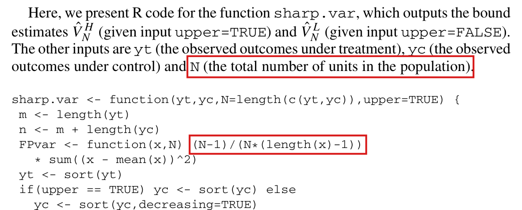
Called with N=Inf, the printed function returns NaN; the infinite-population estimate sT2/m+sC2/(n−m)s_T^2/m+s_C^2/(n-m) requires a branch of its own.

Appendix B, description of the argument N and R code of sharp.var, p. 869 (PDF p. 20); the statements about N=∞N=\infty on pp. 850 and 852 are correct

See also under Formal statements (Lean): P022-T10

As printed

Appendix B, p. 869. The other inputs are yt (the observed outcomes under treatment), yc (the observed outcomes under control) and N (the total number of units in the population).

FPvar <- function(x,N) (N-1)/(N*(length(x)-1))\texttt{FPvar <- function(x,N)~}\colorbox{#ffe58a}{$\texttt{(N-1)/(N*(length(x)-1))}$}

Introduction, p. 850. Our estimator is also applicable to all possible cases of NN and nn (n=N<∞n=N<\infty, n<N<∞n<N<\infty, and N=∞N=\infty), thus providing a unified treatment of the problem.

The problem

The paper says that the estimator covers an infinite population, and that as N→∞N\to\infty with mm and nn fixed it becomes the usual variance estimate for a difference of independent means. Both statements are correct. Appendix B presents sharp.var as the implementation, with N the size of the population, and the value of an infinite N in R is Inf. With N=Inf, the expression in FPvar evaluates Inf/Inf, which is NaN, and the return expression propagates NaN. The function returns NaN for both bounds. The paper documents no call with N=Inf. This is a gap in the code and not a false statement.

Evidence an exact counterexample

I checked an exact example and derived the limit. For treatment and control outcomes (0,1)(0,1) and (0,1)(0,1), the printed function, with the line break in FPvar joined, returns NaN for N=Inf with upper=TRUE and with upper=FALSE. For finite NN it returns (N−2)/(2N)+1/{2(N−1)}(N-2)/(2N)+1/\{2(N-1)\} for the upper bound and (N−2)/(2N)−1/{2(N−1)}(N-2)/(2N)-1/\{2(N-1)\} for the lower bound, that is, 5/125/12 and 1/121/12 at N=4N=4 and 41/9041/90 and 31/9031/90 at N=10N=10, and both expressions tend to 1/21/2. In general, let sT2s_T^2 and sC2s_C^2 be the sample variances with denominators m−1m-1 and k−1k-1, where k=n−mk=n-m. Since FPvar(yt,N)=(N−1)sT2/N\texttt{FPvar(yt,N)}=(N-1)s_T^2/N, the output for finite NN is

(1m−1N)sT2+(1k−1N)sC2+2c^N−1,\Bigl(\frac1m-\frac1N\Bigr)s_T^2+\Bigl(\frac1k-\frac1N\Bigr)s_C^2+\frac{2\hat c}{N-1},

where c^\hat c is the covariance term, which does not depend on NN. Letting N→∞N\to\infty, I obtain sT2/m+sC2/ks_T^2/m+s_C^2/k for both bounds.

What survives

The limit stated on pp. 850 and 852, the formulas for finite NN and the asymptotic results are unaffected. The application has N=n=1561N=n=1561, and the simulations use the same finite population. No reported number involves a call with N=Inf.

Corrected

Join the two lines that define FPvar (P022-E004). After the two lines that define m and n, insert

if (is.infinite(N) && N > 0) return(stats::var(yt)/m + stats::var(yc)/(n-m))\colorbox{#ffe58a}{$\texttt{if (is.infinite(N) \&\& N > 0) return(stats::var(yt)/m + stats::var(yc)/(n-m))}$}

With this line the function returns sT2/m+sC2/(n−m)s_T^2/m+s_C^2/(n-m) for N=Inf in both modes, and every call with finite N is unchanged. The arm sizes m≥2m\ge 2 and n−m≥2n-m\ge 2 assumed on p. 851 make both sample variances well defined. The description may then read: N (the total number of units in the population, or Inf for an infinite population).

The paragraph that introduces the R function sharp.var and the first eight lines of its code. A red box marks the words 'N (the total number of units in the population)'. A second red box marks the expression '(N-1)/(N*(length(x)-1))' in the line that defines FPvar.
Appendix B, p. 869 (PDF p. 20). The upper mark is the description of the argument N; the lower mark is the expression in FPvar that evaluates Inf/Inf when N=Inf.

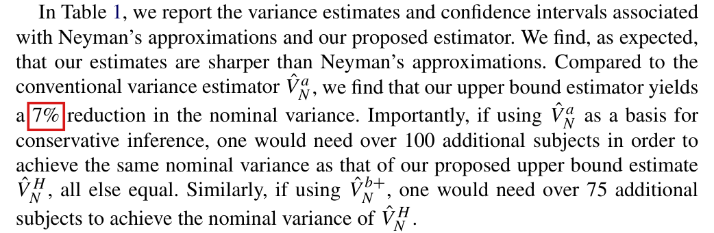
Table 1 puts the reduction in the nominal variance from V^Na\hat V_N^a to V^NH\hat V_N^H at about 6%, not 7%.

Section 6, second paragraph, p. 857 (PDF p. 8), sentence beginning “Compared to the conventional variance estimator”; Table 1, p. 857

See also under Formal statements (Lean): P022-T11

As printed

Compared to the conventional variance estimator V^Na\hat V_N^a, we find that our upper bound estimator yields a 7% reduction in the nominal variance.

The problem

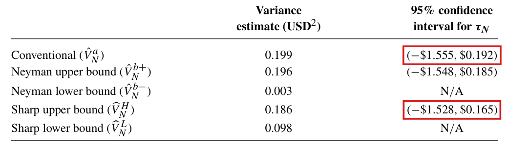
The reduction is D=100 (1−V^NH/V^Na)D = 100\,(1-\hat V_N^H/\hat V_N^a) percent. From the variances printed in Table 1, I find 1−0.186/0.199≈6.53%1-0.186/0.199 \approx 6.53\%, which rounds to 7%. However, each of them is rounded to three decimals, and their rounding can change the whole-percent summary. The 95% confidence intervals in the same table determine the ratio more closely. Both are Wald intervals with the same critical value. The ratio of the two variances is then the square of the ratio of the two half-widths. Allowing for the rounding of every endpoint, the intervals place DD between 5.867 and 6.305. With the variance column as well, DD lies between 6.045 and 6.305, and every value in that range rounds to 6%.

Evidence a historical Lean attribution (Generated status: clause support not certified in this release)

The evidence is a recalculation from Table 1 in exact rational arithmetic. Let aa and hh be the half-widths of the intervals for V^Na\hat V_N^a and V^NH\hat V_N^H. From the printed endpoints, I have a=0.8735a = 0.8735 and h=0.8465h = 0.8465, each to within 0.00050.0005, so that a≤0.8740a\le 0.8740 and h≥0.8460h\ge 0.8460. Since V^NH/V^Na=(h/a)2\hat V_N^H/\hat V_N^a = (h/a)^2, I obtain

V^NHV^Na≥(0.84600.8740)2=178929190969,D≤1204000190969≈6.305<6.5.\frac{\hat V_N^H}{\hat V_N^a} \ge \Bigl(\frac{0.8460}{0.8740}\Bigr)^2 = \frac{178929}{190969}, \qquad D \le \frac{1204000}{190969} \approx 6.305 < 6.5 .

Using the variance column, I have V^NH/V^Na≤0.1865/0.1985=373/397\hat V_N^H/\hat V_N^a \le 0.1865/0.1985 = 373/397, which gives D≥2400/397≈6.045D\ge 2400/397\approx 6.045. The inequality D<6.5D<6.5, under the hypotheses a>0a>0, a≤0.874a\le 0.874 and h≥0.846h\ge 0.846, also has a Lean proof. Since the data of the application are not available, the unrounded value of DD cannot be recovered.

What survives

Table 1 is unchanged, and the two statements that follow the percentage hold. By the same bounds and nominal inverse-sample-size scaling, matching V^NH\hat V_N^H would take between 100.4 and 105.1 additional subjects with V^Na\hat V_N^a, and between 75.3 and 78.5 with V^Nb+\hat V_N^{b+}, in agreement with “over 100” and “over 75”. No formula, proof or other number in the paper uses the percentage.

Corrected

Compared to the conventional variance estimator V^Na\hat V_N^a, we find that our upper bound estimator yields a 6% reduction in the nominal variance.

Nine lines of text from Section 6. A red box marks the figure 7 percent in the sentence which says that the upper bound estimator yields a 7 percent reduction in the nominal variance. The sentences that follow say that over 100 and over 75 additional subjects would be needed.
Section 6, second paragraph, p. 857 (PDF p. 8). The marked figure is the stated reduction in the nominal variance.
Table 1 with five rows. The variance estimates are 0.199, 0.196, 0.003, 0.186 and 0.098. Red boxes mark the confidence intervals (minus 1.555, 0.192) in the row Conventional and (minus 1.528, 0.165) in the row Sharp upper bound.
Table 1, p. 857 (PDF p. 8). The marked cells are the 95% confidence intervals for the conventional estimator and for the sharp upper bound. They determine the ratio of the two variances more closely than the rounded variances do.

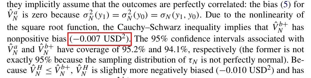
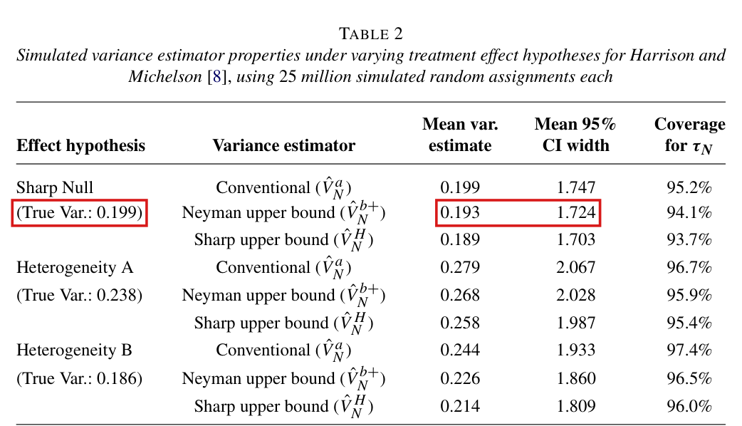
The bias of −0.007-0.007 USD2^2 quoted for V^Nb+\hat V_N^{b+} under the Sharp Null cannot be reconciled with Table 2; the statement that the bias is nonpositive stands without the figure.

Section 6.1, paragraph on the Sharp Null, p. 858 (PDF p. 9); Table 2, Sharp Null block, row “Neyman upper bound”, p. 858

See also under Formal statements (Lean): P022-T12

As printed

Due to the nonlinearity of the square root function, the Cauchy–Schwarz inequality implies that V^Nb+\hat V_N^{b+} has nonpositive bias (−0.007\colorbox{#ffe58a}{$-0.007$} USD2^2).

Table 2, Sharp Null (True Var.: 0.199), row “Neyman upper bound (V^Nb+\hat V_N^{b+})”. Mean var. estimate 0.193; Mean 95% CI width 1.724; Coverage for τN\tau_N 94.1%.

The problem

The bias of a variance estimator is its expectation less the true variance, and the paragraph discusses the 25 million simulated assignments that Table 2 summarizes. For those assignments the table reports a true variance of 0.199, a mean variance estimate of 0.193 for V^Nb+\hat V_N^{b+}, and a mean width of 1.724 for its 95% intervals. A bias that rounds to −0.007-0.007 and a true variance that rounds to 0.199 require a mean variance estimate of at most 0.193. The mean width requires more. Each interval is a Wald interval of full width 2zv2z\sqrt{v}, where vv is the variance estimate, and the square of a mean of square roots is at most the mean. With z=1.96z=1.96, a mean width of at least 1.7235 forces a mean variance estimate of at least 0.193308. The four printed numbers cannot all be rounded summaries of the same simulations with the stated intervals. At least one of them is off in the third decimal, or the intervals were not constructed as stated. The simulation output is needed to say which.

Evidence a historical Lean attribution (Generated status: clause support not certified in this release)

The evidence is an exact calculation from the printed numbers. Let vjv_j be the value of V^Nb+\hat V_N^{b+} in assignment jj, let wj=cvjw_j = c\sqrt{v_j} be the width of its interval, where c=2z0.975c = 2z_{0.975}, and let vˉ\bar v and wˉ\bar w be the means of vjv_j and wjw_j over the simulated assignments. By the Cauchy–Schwarz inequality, I have wˉ2≤c2vˉ\bar w^2\le c^2\bar v. Let VV be the true variance. Since each printed number is rounded to three decimals, I have V≤0.1995V\le 0.1995, wˉ≥1.7235\bar w\ge 1.7235 and vˉ−V≤−0.0065\bar v - V\le -0.0065, so that vˉ≤0.193\bar v\le 0.193. Setting c=3.92c = 3.92, I obtain

vˉ≥1.723523.922=1188180961465600≈0.193308>0.193,vˉ−V≥−0.006192.\bar v \ge \frac{1.7235^2}{3.92^2} = \frac{11881809}{61465600} \approx 0.193308 > 0.193, \qquad \bar v - V \ge -0.006192 .

The contradiction does not depend on the value 1.961.96. The row of Table 1 for V^Nb+\hat V_N^{b+}, with variance 0.196 and interval (−1.548,0.185)(-1.548, 0.185), gives c2≤1.7342/0.1955=44217/2875c^2\le 1.734^2/0.1955 = 44217/2875, which implies that vˉ≥30364623/157216000≈0.193140>0.193\bar v\ge 30364623/157216000\approx 0.193140 > 0.193. The inequality wˉ2≤c2vˉ\bar w^2\le c^2\bar v and the contradiction obtained from the bound on c2c^2 have a Lean proof.

With z=1.96z=1.96, the table summaries bound the simulated bias between −0.006192-0.006192 and −0.005-0.005, so it rounds to −0.006-0.006 or to −0.005-0.005; they do not determine the corrected figure. If the figure −0.007-0.007 is an exact bias computed separately from the simulations of Table 2, the contradiction is not strict. In that case 25 million independent uniform assignments would produce the discrepancy with probability below 10−1010^{-10}.

What survives

The statement that V^Nb+\hat V_N^{b+} has nonpositive bias under the Sharp Null is correct, and V^Na\hat V_N^a is unbiased there. The ordering of the three estimators, the coverage figures and the bias of −0.010-0.010 USD2^2 quoted for V^NH\hat V_N^H are not contradicted by this calculation. None of them was recomputed, since the data are not available. No result of the paper uses the figure.

Corrected

Due to the nonlinearity of the square root function, the Cauchy–Schwarz inequality implies that V^Nb+\hat V_N^{b+} has nonpositive bias (−0.007-0.007 USD2^2).

The difference of the two means printed in Table 2 is 0.193−0.199=−0.0060.193-0.199=-0.006 USD2^2. A figure to three decimals should be taken from the simulation output.

Seven lines of text from Section 6.1. A red box marks the parenthesis 'minus 0.007 USD squared' after the words 'nonpositive bias'. Later in the paragraph the sharp estimator is said to have bias minus 0.010 USD squared.
Section 6.1, paragraph on the Sharp Null, p. 858 (PDF p. 9). The marked parenthesis gives the bias of Neyman’s upper bound estimator.
Table 2 with three blocks of three rows. In the Sharp Null block, red boxes mark 'True Var.: 0.199' and, in the row Neyman upper bound, the mean variance estimate 0.193 and the mean 95 percent CI width 1.724. The coverage in that row is 94.1 percent.
Table 2, p. 858 (PDF p. 9). The marked entries are the true variance under the Sharp Null and, in the row for Neyman’s upper bound, the mean variance estimate and the mean width of the 95% confidence intervals.

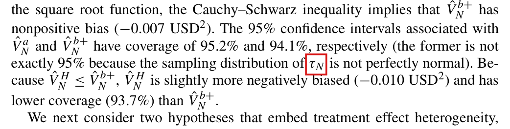
The sampling distribution in the parenthesis is that of the estimator τ^N\hat\tau_N; the hat is missing.

Section 6.1, paragraph on the Sharp Null, p. 858 (PDF p. 9), parenthesis after “95.2% and 94.1%, respectively”

As printed

(the former is not exactly 95% because the sampling distribution of τN\colorbox{#ffe58a}{$\tau_N$} is not perfectly normal)

The problem

The quantity τN\tau_N is the average treatment effect in the population. It is fixed under the design and has no sampling distribution. The parenthesis refers to the difference-in-means estimator τ^N\hat\tau_N defined in (1).

Evidence a check of the printed page

I checked the page at high magnification. The τ\tau carries no hat, while the variance estimators in the neighbouring lines do.

What survives

The coverage figures and the explanation offered for them are unaffected.

Corrected

(the former is not exactly 95% because the sampling distribution of τ^N\colorbox{#ffe58a}{$\hat\tau_N$} is not perfectly normal)

Text from Section 6.1. A red box marks the symbol tau with subscript N, printed without a hat, in the phrase 'the sampling distribution of tau N is not perfectly normal'. The variance estimators in the neighbouring lines carry hats.
Section 6.1, paragraph on the Sharp Null, p. 858 (PDF p. 9). The marked symbol is printed without a hat.

Clarity notes

Imprecise or ambiguous wording whose intended meaning is correct; not an error.

With stochastic potential outcomes, the total variance is at least the expected conditional variance (2), and it is strictly greater only when the population average effect varies.

Section 7, last paragraph, p. 859 (PDF p. 10), sentence beginning “When the potential outcomes are stochastic”

As printed

When the potential outcomes are stochastic, the total variance is greater than the conditional variance (2) because of the additional stochasticity.

Intended meaning

The sentence appeals to the law of total variance. Suppose the potential outcomes YY are random and independent of the assignment, and write VN(Y)V_N(Y) and τN(Y)\tau_N(Y) for the conditional variance (2) and the population average effect given YY. Since EX(τ^N∣Y)=τN(Y)\mathrm{E}_X(\hat\tau_N\mid Y)=\tau_N(Y), I have

Var⁡(τ^N)=EY{VN(Y)}+Var⁡Y{τN(Y)}\operatorname{Var}(\hat\tau_N) = \mathrm{E}_Y\{V_N(Y)\} + \operatorname{Var}_Y\{\tau_N(Y)\}

whenever these variances exist. The total variance is at least the expected conditional variance, and the inequality is strict exactly when Var⁡Y{τN(Y)}>0\operatorname{Var}_Y\{\tau_N(Y)\}>0. This is the comparison the sentence intends, and it is correct. Read literally, the sentence omits the expectation and the case of equality. For example, let N=n=4N=n=4, m=2m=2 and y1=y0=(Z,0,0,0)y_1=y_0=(Z,0,0,0), where ZZ takes the values 00 and 11 with probability 1/21/2 each. Then τN=0\tau_N=0 and VN=Z2/4V_N=Z^2/4, the total variance equals E(VN)=1/8\mathrm{E}(V_N)=1/8, and it is below the conditional variance 1/41/4 when Z=1Z=1. Nothing in the paper depends on the sentence.

Corrected

When the potential outcomes are stochastic and independent of the assignment, and the relevant variances exist, the total variance equals the expected conditional variance (2) plus the variance of the population average effect; it is at least the expected conditional variance, and it is strictly greater when the population average effect varies.

Five lines of text from the last paragraph of Section 7. A red box marks the clause 'total variance is greater than the conditional variance (2)'.
Section 7, last paragraph, p. 859 (PDF p. 10). The marked clause compares the total variance with the conditional variance (2).

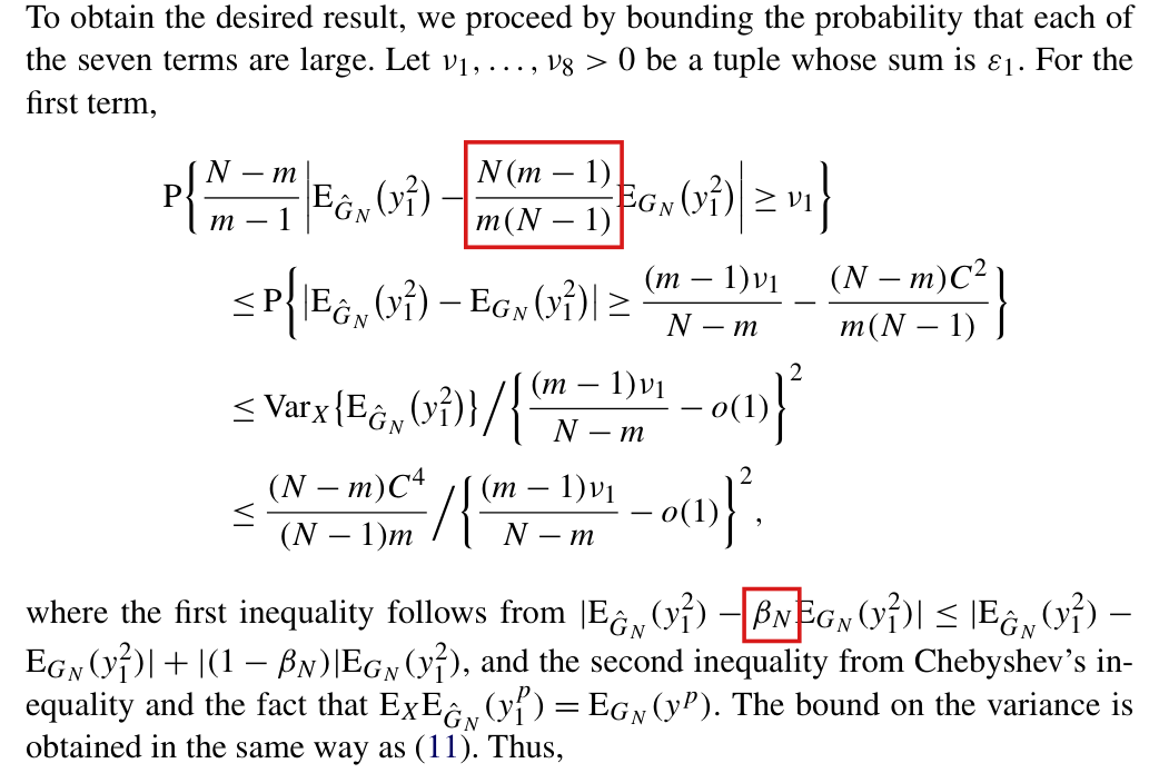
The symbol βN\beta_N stands for the coefficient N(m−1)/{m(N−1)}N(m-1)/\{m(N-1)\} in the display above it; the paper does not define it.

Proof of Proposition 2, bound for the first term, p. 865 (PDF p. 16), sentence beginning “where the first inequality follows from”

As printed

where the first inequality follows from ∣EG^N(y12)−βNEGN(y12)∣|\mathrm{E}_{\hat G_N}(y_1^2)-\colorbox{#ffe58a}{$\beta_N$}\mathrm{E}_{G_N}(y_1^2)| ≤∣EG^N(y12)−EGN(y12)∣{}\le|\mathrm{E}_{\hat G_N}(y_1^2)-\mathrm{E}_{G_N}(y_1^2)| +∣(1−βN)∣EGN(y12){}+|(1-\colorbox{#ffe58a}{$\beta_N$})|\mathrm{E}_{G_N}(y_1^2), and the second inequality from Chebyshev’s inequality and the fact that EXEG^N(y1p)=EGN(yp)\mathrm{E}_X\mathrm{E}_{\hat G_N}(y_1^p)=\mathrm{E}_{G_N}(y^p).

Intended meaning

The symbol βN\beta_N occurs only in this sentence. It abbreviates the coefficient of EGN(y12)\mathrm{E}_{G_N}(y_1^2) in the first line of the display above, that is, βN=N(m−1)/{m(N−1)}\beta_N=N(m-1)/\{m(N-1)\}. With this value, 1−βN=(N−m)/{m(N−1)}1-\beta_N=(N-m)/\{m(N-1)\}, which accounts for the term (N−m)C2/{m(N−1)}(N-m)C^2/\{m(N-1)\} in the second line of the display, and the first inequality holds. In the last identity, yy is the generic argument of the distribution GNG_N, so that EGN(yp)\mathrm{E}_{G_N}(y^p) and EGN(y1p)\mathrm{E}_{G_N}(y_1^p) denote the same moment and the identity is correct as printed.

Corrected

where βN=N(m−1)/{m(N−1)}\colorbox{#ffe58a}{$\beta_N=N(m-1)/\{m(N-1)\}$}, the first inequality follows from ∣EG^N(y12)−βNEGN(y12)∣≤∣EG^N(y12)−EGN(y12)∣+∣(1−βN)∣EGN(y12)|\mathrm{E}_{\hat G_N}(y_1^2)-\beta_N\mathrm{E}_{G_N}(y_1^2)|\le|\mathrm{E}_{\hat G_N}(y_1^2)-\mathrm{E}_{G_N}(y_1^2)|+|(1-\beta_N)|\mathrm{E}_{G_N}(y_1^2), and the second inequality from Chebyshev’s inequality and the fact that EXEG^N(y1p)=EGN(yp)\mathrm{E}_X\mathrm{E}_{\hat G_N}(y_1^p)=\mathrm{E}_{G_N}(y^p).

The bound for the first term in the proof of Proposition 2: a four-line display followed by four lines of text. A red box in the first line of the display marks the fraction N (m minus 1) over m (N minus 1). A second red box in the text marks the symbol beta with subscript N.
Proof of Proposition 2, bound for the first term, p. 865 (PDF p. 16). The lower mark is the first use of βN\beta_N, and the upper mark is the coefficient in the display that it stands for. The symbol recurs once in the next line.

Formal statements (Lean)

Formal results: 15 whole; 1 restricted; 2 refuted; 0 omitted.

Coverage concerns the identified claim under its stated assumptions. A checked proof establishes the formal statement; correspondence to the published text was reviewed by AI. Repository access is currently required to open the source links.

Each result links to its current formal statement and proof. “Whole” covers the identified claim under its assumptions; “restricted” covers the stated narrower scope; “refuted” gives a counterexample to the identified assertion; “omitted” has no current theorem. Any named published theorem used as a premise remains an assumption. Browse the formal results for this work.

Section 6, 'a 7% reduction in the nominal variance' (with Table 1), corrected claim

p. 857 (PDF p. 8)

p. 857 (PDF p. 8). Closed rounding bins and a common positive Wald multiplier imply the endpoint-only upper bound, the combined six-percent bounds, and the exact displayed-input percentage.

Historical component credits
  • Proved AronowAudit.P022.half_width_rounding Historical support retained; baseline fidelity: ok; manifest: used; used in Solution; Auxiliary for the two half-width bins in part (a). Its extra generality is incidental to a valid algebraic rounding fact.
  • Proved AronowAudit.P022.table1_ratio_lower_bound Historical support retained; baseline fidelity: ok; manifest: used; used in Solution; The half-width hypotheses are the very bounds obtained from the endpoint bins; this row is an auxiliary ratio inequality, not an independent rounding model.
  • Proved AronowAudit.P022.table1_corrected_reduction Historical support retained; baseline fidelity: ok; manifest: used; used in Solution; Exactly the combined-bins assertion in part (b). Part (a) does not need the variance bins and is supported separately by the half-width and ratio lemmas; the row is not being treated as a proof under endpoint bins alone.
  • Proved AronowAudit.P022.displayed_variance_reduction Historical support retained; baseline fidelity: ok; manifest: used; used in Solution; Exactly part (c); it does not assert that 1300/199 is the unrounded empirical percentage.

Section 6.1, Sharp Null: the bias '(−0.007-0.007 USD2^2)' of V^Nb+\hat V_N^{b+} (with Table 2), corrected claim

p. 858 (PDF p. 9); Table 1 on p. 857 (PDF p. 8)

p. 858 (PDF p. 9); Table 1 on p. 857 (PDF p. 8). Neyman’s upper estimator has nonpositive sharp-null bias, and the finite Wald-width and rounded-number calculations establish the corrected incompatibility statement.

Historical component credits
  • Proved AronowAudit.P022.finite_sqrt_mean_squared_le_mean Historical support retained; baseline fidelity: ok; manifest: used; used in Solution; The finite Wald-width row directly supplies part (b); its square-root helper is not separately invoked.
  • Proved AronowAudit.P022.finite_wald_mean_width_squared_le Historical support retained; baseline fidelity: ok; manifest: used; used in Solution; Exactly the finite realized-collection inequality in part (b), including negative or zero real multipliers. No population-expectation substitution is made.
  • Proved AronowAudit.P022.table1_multiplier_bound Historical support retained; baseline fidelity: ok; manifest: used; used in Solution; Exactly the algebraic multiplier bound in (c); the theorem assumes rather than silently estimates the width-variance identity.
  • Proved AronowAudit.P022.reported_numbers_incompatible Historical support retained; baseline fidelity: ok; manifest: used; used in Solution; The incompatibility is deterministic only under the target’s explicit same-realized-collection bias interpretation. The Lean premises match that corrected nonexistence claim exactly.
  • Proved AronowAudit.P022.fixed_multiplier_mean_lower Historical support retained; baseline fidelity: ok; manifest: used; used in Solution; Covers the lower-bound component of (e); the separate upper cap there follows directly from its printed bounds on true variance and bias.
  • Proved AronowAudit.P022.Wave1.sharp_null_neyman_bias_proof Historical support retained; baseline fidelity: ok; manifest: used; used in Solution; The conclusion is nonpositive bias, including equality. That is exactly the retained corrected claim, which asserts neither strict negativity nor the deleted numerical bias.

Lemma 2, corrected

p. 860 (PDF p. 11); proof on pp. 860–861 (PDF pp. 11–12)

p. 860 (PDF p. 11); proof on pp. 860–861 (PDF pp. 11–12). Convergence of left limits at atoms gives uniform CDF convergence and both scaled tail bounds with the explicit universal integer function.

Historical component credits
  • Proved AronowAudit.P022.Wave1.TailA.lemma2_corrected_final Historical support retained; baseline fidelity: ok; manifest: not used; not used in Solution; The explicit corrected-lemma row also fixes the universal positive nonincreasing integer function.
  • Proved AronowAudit.P022.PaperDomains.cdf_partition_bracket Historical support retained; baseline fidelity: ok; manifest: not used; not used in Solution; The explicit corrected-lemma row supplies the target; this scalar bracketing helper is not separately invoked.
  • Proved AronowAudit.P022.corrected_partition_integer_properties Historical support retained; baseline fidelity: ok; manifest: used; used in Solution; Its positivity and monotonicity conclusions are already in the explicit corrected-lemma row.
  • Proved AronowAudit.P022.Wave1.lemma2_corrected_explicit_proof Historical support retained; baseline fidelity: ok; manifest: used; used in Solution; The same universal eta can be instantiated separately for each arm, so both eta_1 and eta_0 quantifiers are preserved. The explicit K is independent of H exactly as the corrected target allows.

Lemma 2

p. 860 (PDF p. 11); proof on pp. 860–861 (PDF pp. 11–12)

The printed claim is false: P022-T18; p. 860 (PDF p. 11); proof on pp. 860–861 (PDF pp. 11–12). There exists a sequence satisfying conditions 1–3 for which the joint conclusion of printed Lemma 2 fails.

Historical component credits
  • Counterexample proved AronowAudit.P022.Wave1.lemma2_as_printed_refuted Historical support retained; baseline fidelity: ok; manifest: used; used in Solution; {'source': 'adjudication', 'decision': 'rejected', 'what': 'P022/Wave1/PrintedLemma2.lean:9 negates the universal Conditions123-to-Lemma2Conclusions contract, and P022/P022_Variance.lean:243 does allow K1 and K0 to depend on the experiment and allocation parameters. This weakens the positive assertion relative to the printed dependence on eta and H, so refuting it is stronger and directly refutes the printed lemma as well. Independently of that quantifier difference, the reciprocal witness at P022/P022_Variance.lean:270 satisfies the printed conditions, while P022/P022_Variance.lean:850 states that its population CDF distances equal one for every row, contradicting the uniform-convergence conclusion. The constants cannot affect that failure, so their relaxed dependence creates no material fidelity problem for this refutation.'}

Proof of Proposition 2, the steps that apply Lemma 2, corrected (direct bound for bounded outcomes)

pp. 867–869 (PDF pp. 18–20); statement of Proposition 2 on p. 863 (PDF p. 14)

pp. 867–869 (PDF pp. 18–20); statement of Proposition 2 on p. 863 (PDF p. 14). Bounded outcomes give the stated finite second moments, both deterministic endpoint errors, finite tail bounds, and the allocation-only asymptotic bound.

Historical component credits
  • Proved AronowAudit.P022.Wave1.bounded_direct_finite_proof Historical support retained; baseline fidelity: ok; manifest: used; used in Solution; All sample-size and tolerance conditions match finite parts (a)-(c). Explicit C>=0 is already implied by the bounds on a nonempty population. The empirical-quantile endpoint convention affects only a null set in the integrals.
  • Proved AronowAudit.P022.Wave1.TailA.bounded_direct_asymptotic_final Historical support retained; baseline fidelity: ok; manifest: used; used in Solution; This row covers the asymptotic component, with the finite component covered by R143-19. Metadata inconsistency: P022-T3 has asymptotic=false although its statement expressly includes this asymptotic consequence. ENNReal preserves infinite limsups, and its finite right side is nonnegative.
  • Proved AronowAudit.P022.finite_squared_markov Historical support retained; baseline fidelity: ok; manifest: used; used in Solution; The finite and asymptotic bounded-outcome rows already supply the requested probability bounds.

Equation (11) in the proof of Lemma 2, corrected (with equation (12))

p. 861 (PDF p. 12)

p. 861 (PDF p. 12). Both sampled CDFs are unbiased, have the corrected Bernoulli-factor variances, and satisfy the quarter-factor upper bounds.

Historical component credits
  • Proved AronowAudit.P022.Wave1.cdf_variance_corrected_proof Historical support retained; baseline fidelity: ok; manifest: used; used in Solution; This is the corrected target: the last relation is an inequality. No equality from printed (11) is credited.
  • Proved AronowAudit.P022.bernoulli_variance_bound Historical support retained; baseline fidelity: ok; manifest: used; used in Solution; The corrected CDF-variance row already supplies both quarter-factor upper bounds.
  • Proved AronowAudit.P022.finite_variance_second_moment Historical support retained; baseline fidelity: ok; manifest: used; used in Solution; The indicator-variance row supplies the relevant population-variance identity directly.
  • Proved AronowAudit.P022.indicator_population_variance Historical support retained; baseline fidelity: ok; manifest: used; used in Solution; The statement covers precisely the <= threshold convention and extends it to smaller nonempty populations.
  • Proved AronowAudit.P022.sampled_cdfs_unbiased Historical support retained; baseline fidelity: ok; manifest: used; used in Solution; Both unbiasedness identities are already in the corrected CDF-variance row.

Equation (11) in the proof of Lemma 2, as printed

p. 861 (PDF p. 12)

The printed claim is false: P022-T5; p. 861 (PDF p. 12). The four-unit constant-one example refutes equation (11), and equality in its quarter-factor bound holds exactly when the population CDF is one half.

Historical component credits
  • Proved AronowAudit.P022.finiteMean_const Historical support retained; baseline fidelity: ok; manifest: not used; not used in Solution; The selected aggregate theorem supplies the target component directly; this constituent fact is not separately invoked.
  • Proved AronowAudit.P022.design_constant Historical support retained; baseline fidelity: ok; manifest: not used; not used in Solution; The selected aggregate theorem supplies the target component directly; this constituent fact is not separately invoked.
  • Counterexample proved AronowAudit.P022.equation11_counterexample Historical support retained; baseline fidelity: ok; manifest: used; used in Solution; The witness refutes the universal printed equality. The additional general equality criterion in T5 follows from the corrected variance formula and R144-02; this row describes only the concrete witness.

Appendix B, function sharp.var: partition points and integration weights, corrected

p. 869 (PDF p. 20); equations (8)–(9) on p. 854 (PDF p. 5)

p. 869 (PDF p. 20); equations (8)–(9) on p. 854 (PDF p. 5). Using the original partition widths and midpoint quantile selections returns the sharp covariance and variance estimates, with the stated rank and overlap-weight identities.

Historical component credits
  • Proved AronowAudit.P022.Wave1.appendixB_corrected_proof Historical support retained; baseline fidelity: ok; manifest: used; used in Solution; Matches the corrected exact-arithmetic target, including both covariance endpoints and overlap masses. No assertion about floating-point execution is part of this target.
  • Proved AronowAudit.P022.centered_quadrature Historical support retained; baseline fidelity: ok; manifest: not used; not used in Solution; The corrected Appendix B row already supplies the centered covariance and variance substitution identities.

Appendix B, function sharp.var, as printed

p. 869 (PDF p. 20); equations (8)–(9) on p. 854 (PDF p. 5)

The printed claim is false: P022-T9; Appendix B, p. 869 (PDF p. 20), (8)–(9) on p. 854. In real arithmetic the all-ones four-unit example has constant observed samples, zero effect, variance and sharp estimates, but the printed routine returns the negative value -1/50331648. Its shifted weights sum to 1-2e. Under the stated cell-width condition both endpoint discrepancies and the exact translation defect hold, while the mathematical sharp estimates are translation invariant. The usual measure-theoretic conditions are assumed.

Historical component credits
  • Proved AronowAudit.P022.partition_two Historical support retained; baseline fidelity: ok; manifest: used; used in Solution; The selected aggregate theorem supplies the target component directly; this constituent fact is not separately invoked.
  • Proved AronowAudit.P022.quantile_two_ones Historical support retained; baseline fidelity: ok; manifest: used; used in Solution; The selected aggregate theorem supplies the target component directly; this constituent fact is not separately invoked.
  • Proved AronowAudit.P022.sharp_covariance_two_ones Historical support retained; baseline fidelity: ok; manifest: used; used in Solution; The selected aggregate theorem supplies the target component directly; this constituent fact is not separately invoked.
  • Counterexample proved AronowAudit.P022.appendixB_counterexample Historical support retained; baseline fidelity: ok; manifest: used; used in Solution; This is a witness for failure of the printed routine, not a proof of its positive correctness claim. All printed witness hypotheses hold, including the permitted constant outcomes and census design.
  • Proved AronowAudit.P022.Wave1.appendixB_general_discrepancy_proof Historical support retained; baseline fidelity: ok; manifest: used; used in Solution; Auxiliary general-discrepancy component; both discrepancy equalities are exported. The real-arithmetic model and width restriction are already explicit in the target, so neither is an extra Lean assumption.

The infinite-population case (N=∞N = \infty) of the estimator: Introduction and Section 2, and Appendix B called with N=Inf, corrected claim

p. 850 (PDF p. 1); p. 852 (PDF p. 3); Appendix B, p. 869 (PDF p. 20)

p. 850 (PDF p. 1); p. 852 (PDF p. 3); Appendix B, p. 869 (PDF p. 20). Fixed observed samples give the independent-means estimator limit, and bounded marginal variances with eventual fixed arm sizes give the corresponding actual-variance approximation.

Historical component credits
  • Proved AronowAudit.P022.fixed_sample_identity Historical support retained; baseline fidelity: ok; manifest: used; used in Solution; This is the mathematical fixed-sample identity in part (a), with no claim to execute an R branch at an infinite argument.
  • Proved AronowAudit.P022.fixed_sample_infinite_limit Historical support retained; baseline fidelity: ok; manifest: used; used in Solution; This proves the mathematical independent-means estimator limit for both modes; finite exceptional natural population sizes are irrelevant.
  • Proved AronowAudit.P022.independent_means_remainder Historical support retained; baseline fidelity: ok; manifest: used; used in Solution; This is algebra for varianceExpression; the restricted theorem does not assert its exact identity for actual variance.
  • Proved AronowAudit.P022.Wave1.fixed_arm_variance_limit_eventually Historical support retained; baseline fidelity: ok; manifest: used; used in Solution; Eventually constant arm sizes correctly avoid the artificial all-row restriction caused by starting the sequence at N=4. The corrected target itself supplies the bounded-variance condition; no positive limiting sampling fraction is assumed.

Lemma 1 (Hoeffding) and the sentence 'Lemma 1 implies that [VNL,VNH][V_N^L, V_N^H] is the sharpest interval bound for VNV_N'; with equation (2)

p. 853 (PDF p. 4); equation (2) on p. 851 (PDF p. 2); proof of Lemma 1 on pp. 859–860 (PDF pp. 10–11)

p. 853 (PDF p. 4); equation (2) on p. 851 (PDF p. 2); proof of Lemma 1 on pp. 859–860 (PDF pp. 10–11). Difference in means is unbiased with the printed variance, and the covariance and variance endpoints bound and attain all compatible finite rearrangements and probability couplings.

Historical component credits
  • Proved AronowAudit.P022.Wave1.sharp_bounds_variance_and_all_couplings Historical support retained; baseline fidelity: ok; manifest: used; used in Solution; {'source': 'adjudication', 'decision': 'rejected', 'what': 'P022/Wave1/SharpBounds.lean:24 includes unbiasedness, the actual assignment-variance identity, bounds for every population with the given marginal multisets, endpoint attainment, and covariance bounds and quantile-law attainment for every compatible Borel probability coupling. Design at P022/P022_Variance.lean:13 imposes precisely the standing population and arm-size conditions, and uniform permutations give each unordered assignment the same multiplicity. Equality of all bounded continuous test integrals specifies the printed equality in distribution, while the quantile endpoint totalization changes no uniform law or integral. None of the noted representations narrows Lemma 1 or the sharp variance interval claim.'}
  • Proved AronowAudit.P022.finite_covariance_cauchy Historical support retained; baseline fidelity: ok; manifest: not used; not used in Solution; The selected aggregate theorem supplies the target component directly; this constituent fact is not separately invoked.
  • Proved AronowAudit.P022.permutation_eval_mean Historical support retained; baseline fidelity: ok; manifest: used; used in Solution; The selected aggregate theorem supplies the target component directly; this constituent fact is not separately invoked.
  • Proved AronowAudit.P022.observed_means_unbiased Historical support retained; baseline fidelity: ok; manifest: used; used in Solution; The selected aggregate theorem supplies the target component directly; this constituent fact is not separately invoked.
  • Proved AronowAudit.P022.difference_in_means_unbiased Historical support retained; baseline fidelity: ok; manifest: used; used in Solution; The selected aggregate theorem supplies the target component directly; this constituent fact is not separately invoked.

Section 3, sentence after equation (9): V^NH\hat V_N^H is never greater than V^Nb+\hat V_N^{b+}, and V^NL\hat V_N^L is never smaller than V^Nb−\hat V_N^{b-}

p. 854 (PDF p. 5); (4) and (6) on pp. 852–853 (PDF pp. 3–4); Introduction, p. 850 (PDF p. 1)

p. 854 (PDF p. 5); (4) and (6) on pp. 852–853 (PDF pp. 3–4); Introduction, p. 850 (PDF p. 1). When the full population is sampled, every assignment obeys the five-estimator ordering from Neyman’s lower estimate through the conventional upper estimate.

Historical component credits
  • Proved AronowAudit.P022.Wave1.estimated_bound_ordering_proof Historical support retained; baseline fidelity: ok; manifest: used; used in Solution; The quantified pointwise ordering is fully established. The introductory phrase often smaller carries no frequency quantifier in the target formal reading.
  • Proved AronowAudit.P022.sqrt_product_le_arithmetic Historical support retained; baseline fidelity: ok; manifest: used; used in Solution; The selected aggregate theorem supplies the target component directly; this constituent fact is not separately invoked.

Proposition 1

p. 855 (PDF p. 6); proof on pp. 862–863 (PDF pp. 13–14)

p. 855 (PDF p. 6); proof on pp. 862–863 (PDF pp. 13–14). Conditions 1–4 give second moments for all compatible laws, both sharp population limits, and joint bound-estimator consistency at scale one over population size.

Historical component credits
  • Proved AronowAudit.P022.Wave1.TailB_proposition1 Historical support retained; baseline fidelity: ok; manifest: used; used in Solution; All moment and consistency claims are conclusions of the inherited theorem type, not assumptions inside a structure. Coordinate second moments bound every compatible covariance range, so sSup/sInf and Bochner integrals have their intended meanings. No additional left-CDF convergence at atoms is assumed.

Proposition 2 (with Remark 3)

p. 863 (PDF p. 14); Remark 3 on p. 856 (PDF p. 7); proof on pp. 863–869 (PDF pp. 14–20)

p. 863 (PDF p. 14); Remark 3 on p. 856 (PDF p. 7); proof on pp. 863–869 (PDF pp. 14–20). Bounded outcomes give both stated scaled tail limit-superior bounds uniformly over admissible sequences with the same limiting law and allocation parameters.

Historical component credits
  • Proved AronowAudit.P022.Wave1.proposition2_proof Historical support retained; baseline fidelity: ok; manifest: used; used in Solution; {'source': 'adjudication', 'decision': 'rejected', 'what': 'P022/Wave1/Gap/GP022B1b.lean:1001 supplies both endpoint bounds for every positive tolerance allocation under Conditions123 and uniformly bounded outcomes. Conditions123 at P022/P022_Variance.lean:194 contains the printed conditions 1–3 without an extra left-limit or uniform-CDF assumption, and scaledProbabilityLimsup at :233 is the extended-real limsup of N times the actual assignment probability. Finite nonnegative κ functions are chosen before the sequence and tolerance allocation with only the parameter dependencies permitted by the target. The lower bound with outside coefficient one strengthens the allowed finite-constant bound, and N = q + 4 merely indexes all population sizes in the standing setting; neither difference removes any case.'}

Corollary 1 (with Remark 4)

p. 856 (PDF p. 7); Remark 4 on p. 857 (PDF p. 8)

Corollary 1, p. 856 (PDF p. 7), Remark 4, p. 857 (PDF p. 8). Conditions 1–3, uniformly bounded third moments and a nonsingular limiting law give the actual and upper variance limits, gamma in (0,1], the studentized normal limit, and the stated Wald coverage limit at least nominal. No positivity of every finite estimate is assumed; division is totalized on exceptional rows. The sharp upper variance is the least leading variance input assuring nominal Wald coverage uniformly over admissible joint laws with the given marginals. Every smaller nonnegative input is defeated by a nonsingular compatible law and a nested fixed-outcome population realizing it. The usual measure-theoretic conditions are assumed, and existence of the moments and extrema is concluded.

Historical component credits
  • Proved AronowAudit.P022.Wave1.TailB_corollary1_and_coverage Limited support; baseline fidelity: narrower; manifest: used; used in Solution; {'source': 'adjudication+second review', 'adjudicator': 'P022/Wave1/Gap/TailBCorollaryCoverage.lean:199 copies the type of corollary1_and_coverage at P022/P022_Variance.lean:764, whose conclusions establish the CLT, variance limit, and nominal-coverage inequality but contain no optimality assertion. The supplied target additionally says in Remark 4 that the interval is “asymptotically the narrowest Wald-type confidence interval assured to have at least the nominal coverage.” Showing coverage of this interval does not establish that every smaller marginal-based variance input fails to guarantee coverage across compatible joint laws. The record and row descriptions expressly exclude that conclusion, but this exclusion does not amend the supplied claim text; the reviewer correctly identified the omission but understated its severity. The finite-variance and square-root totalizations themselves are harmless under the positive limiting variance and consistency.', 'suggested_fix': 'Add an optimality conclusion: any asymptotic variance input determined only by the marginal laws that is strictly smaller than the sharp upper variance limit fails to guarantee nominal Wald coverage for some admissible compatible joint law. The quantification must cover alternative variance inputs and compatible laws, using endpoint attainment or admissible approximation where needed; the current coverage inequality alone is insufficient.', 'second_review': "P022/Wave1/Gap/TailBCorollaryCoverage.lean:199 takes the type of corollary1_and_coverage at P022/P022_Variance.lean:764, which concludes the CLT, variance limit, and coverage limit and inequality but no optimality assertion. Target T17 expressly includes Remark 4's claim that the interval is 'asymptotically the narrowest Wald-type confidence interval assured to have at least the nominal coverage'; the exclusion in the row description does not remove that target requirement. Although limitingBound uses a supremum over compatible laws at P022/P022_Variance.lean:672, the exported theorem does not establish that a smaller marginal-based variance input loses the coverage guarantee for an admissible compatible law. A substantive optimality conclusion is therefore needed in addition to the existing coverage conclusions.", 'severity': 'major'}
  • Proved AronowAudit.P022.third_moment_tail_bound Historical support retained; baseline fidelity: ok; manifest: used; used in Solution; The exact narrowed corollary row supplies the CLT and coverage conclusions directly.
  • Proved AronowAudit.P022.allocation_coefficient_product Historical support retained; baseline fidelity: ok; manifest: used; used in Solution; The exact narrowed corollary row supplies the CLT and coverage conclusions directly.

Lemma 2, as printed

p. 860 (PDF p. 11); proof on pp. 860–861 (PDF pp. 11–12)

The printed claim is false: P022-T1; p. 860 (PDF p. 11), proof on pp. 860–861. The fixed negative-reciprocal witness satisfies conditions 1–4 but has population and sample CDF error one, certain tails, and a persistent error at the required partition knot zero. The bounded perturbed four-corner witness satisfies conditions 1–4 with a nonsingular limit and has CDF error at least one half and certain tails. Thus both conclusions of printed Lemma 2 fail, even with a nonsingular limiting law. The usual measure-theoretic conditions are assumed.

Historical component credits
  • Proved AronowAudit.P022.empirical_cdf_bounds Historical support retained; baseline fidelity: ok; manifest: used; used in Solution; The selected aggregate theorem supplies the target component directly; this constituent fact is not separately invoked.
  • Proved AronowAudit.P022.origin_cdf Historical support retained; baseline fidelity: ok; manifest: used; used in Solution; The selected aggregate theorem supplies the target component directly; this constituent fact is not separately invoked.
  • Proved AronowAudit.P022.zero_atom_distance Historical support retained; baseline fidelity: ok; manifest: used; used in Solution; The selected aggregate theorem supplies the target component directly; this constituent fact is not separately invoked.
  • Proved AronowAudit.P022.reciprocal_below_threshold Historical support retained; baseline fidelity: ok; manifest: used; used in Solution; The selected aggregate theorem supplies the target component directly; this constituent fact is not separately invoked.
  • Proved AronowAudit.P022.reciprocal_finite_errors Historical support retained; baseline fidelity: ok; manifest: used; used in Solution; The selected aggregate theorem supplies the target component directly; this constituent fact is not separately invoked.
  • Proved AronowAudit.P022.reciprocal_atom_values Historical support retained; baseline fidelity: ok; manifest: used; used in Solution; The selected aggregate theorem supplies the target component directly; this constituent fact is not separately invoked.
  • Proved AronowAudit.P022.reciprocal_outcome_limit Historical support retained; baseline fidelity: ok; manifest: used; used in Solution; The selected aggregate theorem supplies the target component directly; this constituent fact is not separately invoked.
  • Proved AronowAudit.P022.reciprocal_weak_limit Historical support retained; baseline fidelity: ok; manifest: used; used in Solution; The selected aggregate theorem supplies the target component directly; this constituent fact is not separately invoked.
  • Proved AronowAudit.P022.reciprocal_allocation_limit Historical support retained; baseline fidelity: ok; manifest: used; used in Solution; The selected aggregate theorem supplies the target component directly; this constituent fact is not separately invoked.
  • Proved AronowAudit.P022.origin_cdf_continuous_off_atom Historical support retained; baseline fidelity: ok; manifest: used; used in Solution; The selected aggregate theorem supplies the target component directly; this constituent fact is not separately invoked.
  • Proved AronowAudit.P022.reciprocal_conditions123 Historical support retained; baseline fidelity: ok; manifest: used; used in Solution; The selected aggregate theorem supplies the target component directly; this constituent fact is not separately invoked.
  • Proved AronowAudit.P022.reciprocal_tail_diverges Limited support; baseline fidelity: narrower; manifest: used; used in Solution; Used only through the aggregate counterexample: its exact statement is the infinite limsup, without a standalone probability-one conclusion.
  • Counterexample proved AronowAudit.P022.lemma2_counterexample Historical support retained; baseline fidelity: ok; manifest: used; used in Solution; This is an exact witness for the printed universal lemma, not a positive proof of it. Witness B and the optional condition-4 observation are unnecessary for this refutation and are not separately asserted here.

Proof of Proposition 2: tolerance of the last term, equation (23) and the concluding display for V^NH\hat V_N^H, corrected

pp. 865 and 867–868 (PDF pp. 16 and 18–19); statement of Proposition 2 on p. 863 (PDF p. 14)

pp. 865 and 867–868 (PDF pp. 16 and 18–19), Proposition 2 on p. 863. The corrected upper seven-term budget uses sum nu=epsilon1/2 and last tolerance epsilon1/2, and is centered at the sharp upper bound. The finite decomposition, event inclusion, union bound and last-term CDF bound hold. Conditional on the Lemma 2 conclusions, universal positive nonincreasing integer functions give the corrected last-term limit; conditional also on (17)–(22), the concluding bounds hold. The cubic-root allocation attains their minimum and gives a positive rate function independent of the sequence. The lower endpoint retains sum nu=epsilon1 and last tolerance epsilon2+epsilon3, with its decomposition, finite budget and conditional limits. The reciprocal thresholds require C>0; at C=0 both last integrals vanish. The usual measure-theoretic conditions are assumed.

Historical component credits
  • Proved AronowAudit.P022.corrected_allocation_sum Historical support retained; baseline fidelity: ok; manifest: used; used in Solution; The omitted sign assumptions strengthen the auxiliary algebraic identity.
  • Proved AronowAudit.P022.seven_total_abs_le Historical support retained; baseline fidelity: ok; manifest: used; used in Solution; The event-inclusion glue invokes seven_term_budget, which already incorporates this triangle bound.
  • Proved AronowAudit.P022.seven_term_budget Historical support retained; baseline fidelity: ok; manifest: used; used in Solution; This is the deterministic event-inclusion lemma; R144-09 relates the signed total to the estimator and supplies the probability inequality.
  • Proved AronowAudit.P022.Wave1.proposition2_corrected_finite_proof Historical support retained; baseline fidelity: ok; manifest: used; used in Solution; Covers the finite H-endpoint parts (a)-(b), including the decomposition. The pointwise event inclusion also follows directly by combining its identity with R144-12.
  • Proved AronowAudit.P022.Wave1.proposition2_corrected_limit_proof Historical support retained; baseline fidelity: ok; manifest: used; used in Solution; This is the fixed-xi conditional assembly in T6(c)-(d), not a proof of printed Lemma 2, a minimization theorem, or a law-only constant uniform in all sequences and parameters. The selected K positivity/monotonicity is not itself a conclusion of this covered component. These limitations were already recognized in the blind backtranslation and claim-stage judgment.

Proof of Proposition 2: equation (23) and the concluding display for V^NH\hat V_N^H, as printed

p. 868 (PDF p. 19); statement of Proposition 2 on p. 863 (PDF p. 14)

The printed claim is false: P022-T7; p. 868 (PDF p. 19), Proposition 2 on p. 863. The nested four-corner population satisfies the stated assumptions. The admissible split (1,1,1) makes (23) a probability-one event. On N=4r the exact moments give a scaled centering gap tending to one half; the centered error has the stated 51200/(N delta^2) tail bound. The wrongly centered absolute error tends to one half in probability, its small-threshold probabilities tend to one, and their N-scaled values diverge, refuting both finite printed bounds. The usual measure-theoretic conditions are assumed.

Historical component credits
  • Proved AronowAudit.P022.Wave1.proposition2_printed_counterexample_proof Historical support retained; baseline fidelity: ok; manifest: used; used in Solution; At epsilon1=epsilon2=epsilon3=1 and epsilon=3, printed (23) has a certain zero-threshold event. For the separate wrong-V_N display, choose any 0<epsilon<1/2 and admissible positive tolerance split: its asserted finite upper bound contradicts the stated infinite subsequence limsup. This does not refute the correctly centered Proposition 2.
  • Proved AronowAudit.P022.zero_tolerance_tail Historical support retained; baseline fidelity: ok; manifest: used; used in Solution; The four-corner counterexample supplies both refutations directly; this general mechanism is not separately invoked.
  • Counterexample proved AronowAudit.P022.equation23_counterexample Historical support retained; baseline fidelity: ok; manifest: not used; not used in Solution; The selected four-corner witness handles both displays; this supplementary zero-population witness handles only equation (23).

Reproduction

What I recalculated or reran from public materials. "Agrees", "Agrees in part" or "Disagrees" compares my result with the printed one. "Not compared" means the comparison could not be made.

Status
Selected recalculation
Agreement
Agrees in part
Reported results that were targeted
TargetWhereMethodStatusAgreement
Table 1 and application estimatesp. 857 (PDF p. 8)I could not regenerate the application estimates without the Harrison and Michelson data. The Blocked and Not compared labels refer to that data-based rerun. I checked the printed table for internal consistency; the separate efficiency row reports the comparison of its variance-reduction and additional-subject claims.BlockedNot compared
Application efficiency claimsp. 857 (PDF p. 8)I recalculated the application efficiency claims from Table 1. The printed variances and confidence intervals together bound the variance reduction between 6.045% and 6.305%, assuming Wald intervals with a common critical value, so it rounds to 6%, rather than the reported 7% (P022-N003). Under nominal inverse-sample-size scaling, the additional-subject bounds are about 100.4–105.1 and 75.3–78.5, supporting “over 100” and “over 75”. I could not regenerate the underlying estimates without the application data.RecalculatedAgrees in part
Table 2p. 858 (PDF p. 9); hypotheses continued p. 859 (PDF p. 10)I recalculated internal relationships from the printed numbers: the mean interval widths are compatible with the mean variance estimates, and the Heterogeneity A true variance and mean conventional estimate follow from the Sharp Null variance and the ten modified outcomes. The quoted Sharp Null bias of −0.007 USD² for the Neyman upper bound cannot be reconciled with Table 2 (P022-N005); the replacement figure requires the simulation output. The table relationships agree; partial agreement reflects the incompatible quoted bias figure. I could not rerun the simulations without the experiment data and simulation code.RecalculatedAgrees in part
Table 3p. 870 (PDF p. 21), setup p. 869 (PDF p. 20)I recalculated all 36 ratios by numerical integration of the reported Beta quantile functions, using new R code. Every ratio agrees to the printed two decimals; I did not rerun the original Mathematica calculation.RecalculatedTo rounding