P023-E001 Moderate
Full-sample OLS with the coarsened control of Proposition 1 relies solely on outcomes from close elections; a polynomial regression can estimate the same jump at the threshold while also using distant outcomes.
Section 1, p. 3 (PDF p. 3), paragraph continued from p. 2; repeated in the last paragraph of Section 3.2, p. 7, and in the second sentence of Section 5, p. 8
Classification before my review (the classification when the audit was first completed, before I reviewed it): Error, Major (entry P023-E001).
See also under Formal statements (Lean): P023-T1, P023-T2, P023-T3, P023-T10
I disputed this classification, but as a rule, deferred to the models’ final judgment: see my comment and the history of this entry.
As printed
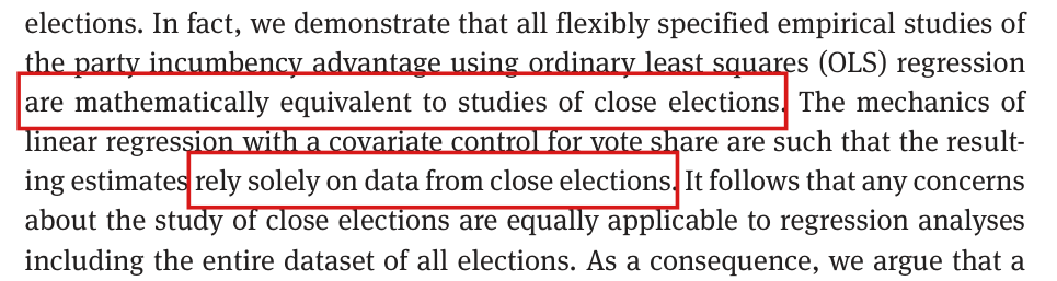
[p. 3] “In fact, we demonstrate that all flexibly specified empirical studies of the party incumbency advantage using ordinary least squares (OLS) regression are mathematically equivalent to studies of close elections. The mechanics of linear regression with a covariate control for vote share are such that the resulting estimates rely solely on data from close elections. It follows that any concerns about the study of close elections are equally applicable to regression analyses including the entire dataset of all elections.”
[p. 7] “Since the RD estimator only uses information from close elections to estimate causal effects, it is also generally the case that the OLS estimator, when well-specified, will also only use information from close elections to estimate causal effects.”
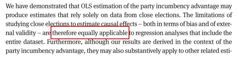
[p. 8] “We have demonstrated that OLS estimation of the party incumbency advantage may produce estimates that rely solely on data from close elections. The limitations of studying close elections to estimate causal effects – both in terms of bias and of external validity – are therefore equally applicable to regression analyses that include the entire dataset.”
The problem
The paper distinguishes two results. Proposition 1 concerns the regression whose controls are indicators for bins of width of the margin , the “coarsened control” of Table 1; I call it the coarsened regression. Its OLS coefficient equals the difference in means within the window , and every outcome outside the window has weight zero in it. Proposition 2 concerns regressions with a polynomial in the margin, such as the linear and degree-7 controls of Table 1. Appendix B compares the polynomial and shrinking-window RD estimates through the cutoff jump , rather than through their observation weights.
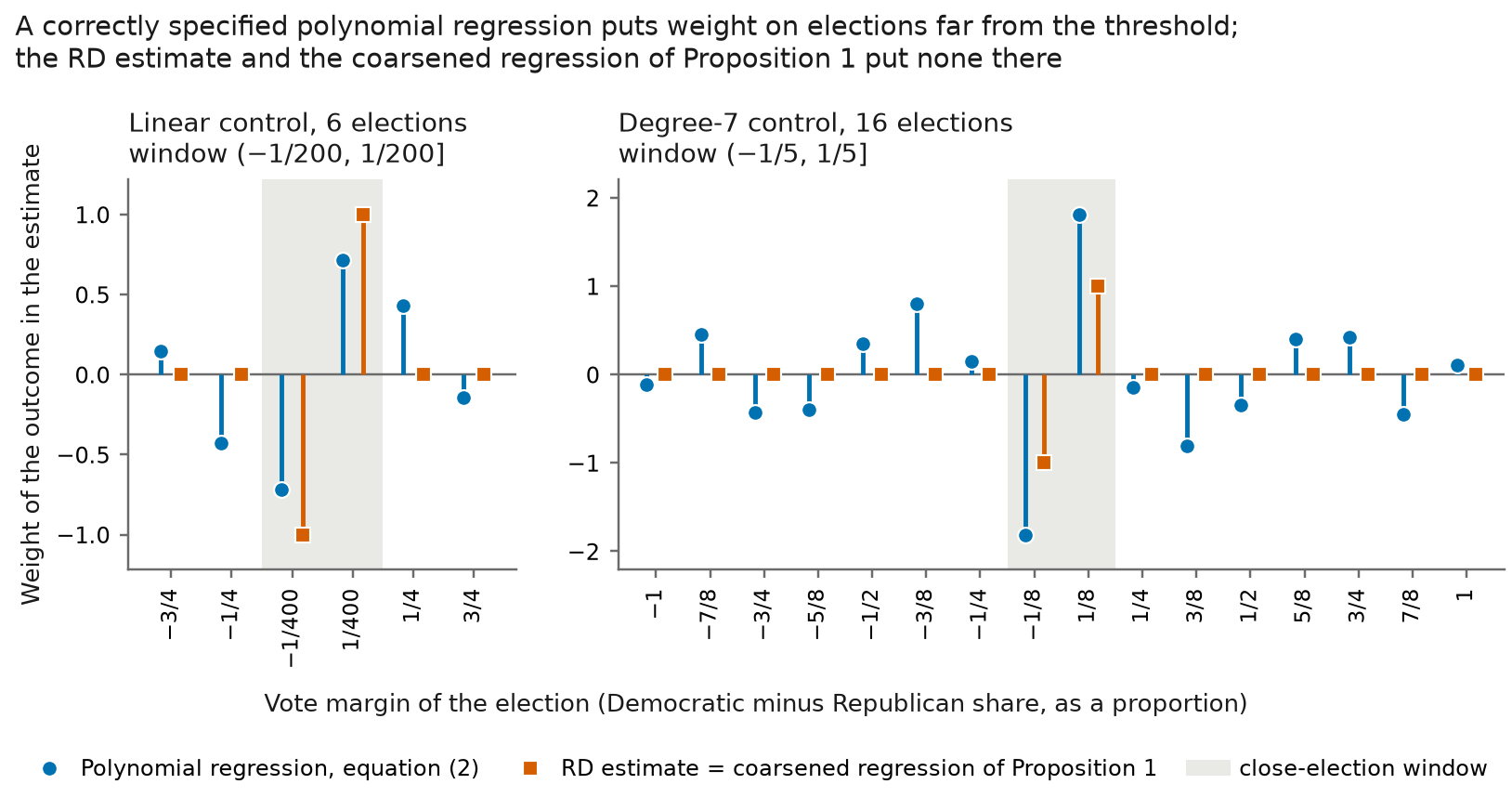
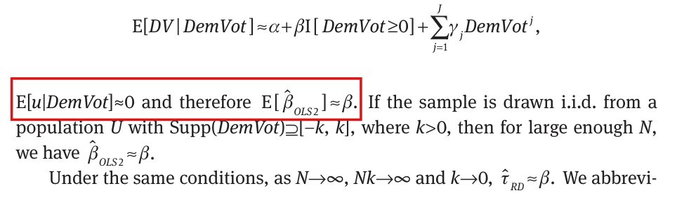
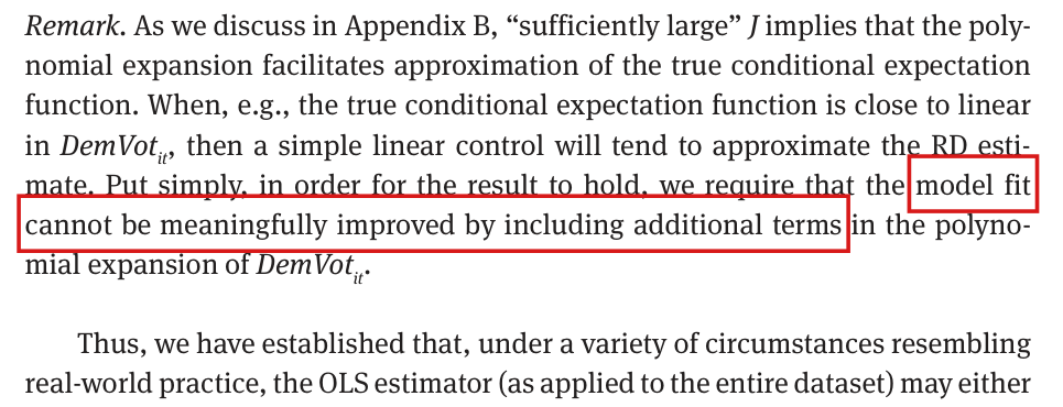
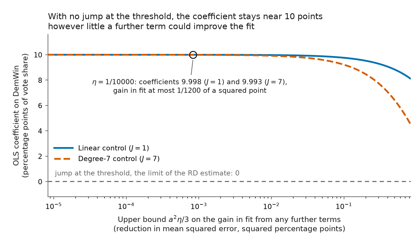
Read as a whole, the paper separates exact coarsened equivalence from approximate polynomial equivalence in large samples. The phrase “mathematically equivalent” on p. 3 should be read in that context. Nevertheless, the explanation in terms of the mechanics of regression, followed by “rely solely on data” on p. 3 and “only use information” on p. 7, naturally asserts exclusive dependence on close-election outcomes. That assertion is false for the permitted finite polynomial controls. Its failure does not demonstrate failure of either equivalence result. The identified coefficient of a polynomial regression of degree is a weighted sum over all elections. The weight is proportional to the residual of on the polynomial terms, and this residual is nonzero at all but at most distinct margins. Raising the outcome of a distant election with nonzero weight then changes the estimate, even when the polynomial model is exactly correct, while the RD estimate and the coefficient of the coarsened regression do not move.
Two estimators with the same limit need not have the same weights, the same sampling variance or the same bias at a fixed bandwidth. Under shared consistency their difference nevertheless converges to zero in probability; nonzero distant weights do not refute that approximation. For the coarsened regression, equality of the estimators transfers the properties of the specified RD estimate directly. For polynomial controls, Appendix B already supplies the common-target argument, and Section 2 describes assumptions needed for its causal interpretation. Different outcome weights do not remove concerns that arise from that common target and those assumptions. They establish neither different causal bias nor broader external validity in the application.
Evidence an exact counterexample
The evidence is a derivation, two exact counterexamples and a recalculation of the weights on the available House replication data. Let be the residual of the vector after least-squares projection on the constant and the powers . For an identified coefficient in equation (2), I obtain from the normal equations
which implies that raising one outcome by changes the estimate by .
For the linear control (), take six elections with margins , , , , , and outcomes . Equation (2) then holds exactly with . In the order of the margins, the weights are
With , only the elections at lie in the window. For the degree-7 control, take sixteen elections with margins and outcomes . Equation (2) with holds exactly, again with , and the sixteen weights, in increasing order of margin, are
none of them zero. With , only the elections at lie in the window. The table shows what happens when the outcome of the election with the largest margin ( in the first example, in the second) is raised by .
| Estimate | Before | After | Change |
|---|---|---|---|
| Polynomial regression, | |||
| RD, coarsened regression, | |||
| Polynomial regression, | |||
| RD, coarsened regression, |
In each example the two outcome vectors are realizations of one correctly specified model. Take errors independent of one another and of the margins, with probabilities , and at , and . Conditional on the stated margins, the baseline and perturbed error vectors have probabilities and in the six-election example, and and in the sixteen-election example. These probabilities establish that the outcomes are possible under the same conditional-mean model; they do not measure the probability of an OLS–RD discrepancy exceeding a fixed positive amount. The finite designs themselves do not test a shrinking-bandwidth asymptotic claim.
The targets do agree. For margins uniform on and the same two conditional means, the population coefficient of equation (2) is , and the difference in means within bandwidth is for and for , which tends to as . With independent observations, the bounded mean-zero errors just specified and, for example, , both estimators are consistent for . The finite grids are used for conditional sensitivity calculations; no positive probability of drawing those exact grids from a continuous distribution is asserted.
More generally, whenever both estimators converge in probability to the same , for each fixed the triangle inequality gives
This requires no independence between the estimators. It does not assert equality at finite sample sizes, a probability for a particular sample size, or equivalence after division by a shrinking standard error.
Their variance contributions can still differ. With homoskedastic errors, elections whose margins have absolute value at least contribute of the leading error variance of the coefficient of equation (2) for and (about 5.6%) for . The leading contribution from the errors to the variance is for and for , against for the difference in means with . The polynomial contributions vanish at order , so their positive distant shares do not imply a persistent discrepancy between the estimates.
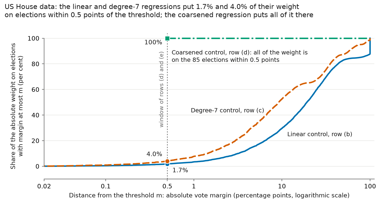
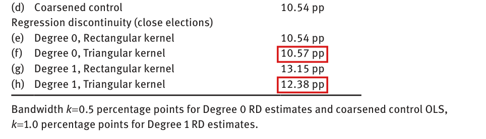
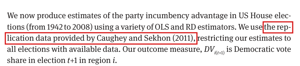
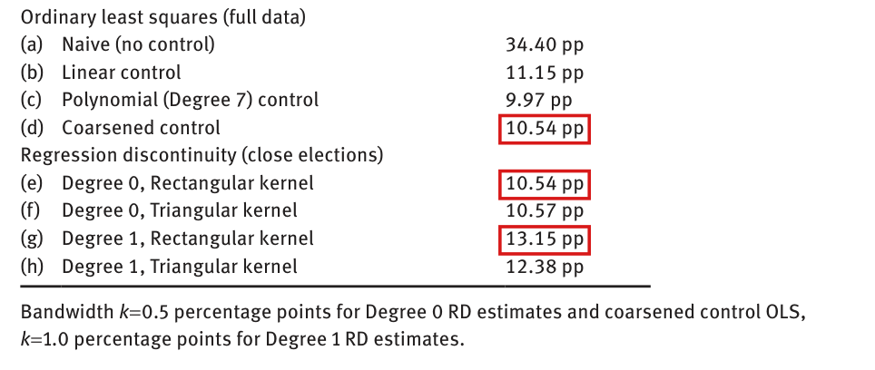
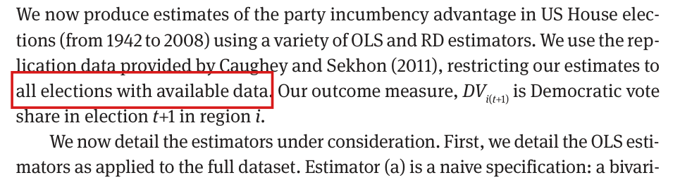
On the available House replication data, the two polynomial specifications of Table 1 also put most of their weight on distant elections. In the 2014 release of the replication data of Caughey and Sekhon (2011), 8,610 elections from 1942–2008 have the outcome (DPctNxt), the margin (DifDPct) and the winner (DemWin) recorded, and a recalculation in exact arithmetic gives the weights for the specifications of rows (b) and (c) on these elections. The available codebook defines this margin as the leading Democrat’s percentage minus the leading non-Democrat’s, rather than a two-party renormalization. The 85 elections within 0.5 points of the threshold form the window of rows (d) and (e). They carry 1.7% of for the linear control and 4.0% for the degree-7 control. Each of the other 8,525 elections has a nonzero weight in both regressions, and the elections decided by more than 10 points carry 70% and 47% of . In the coarsened specification of row (d), the 85 elections carry all of the weight. The three coefficients are nonetheless close: 11.15, 9.95 and 10.54 points. With the sample restricted to the 8,594 elections flagged Use=1 for Caughey and Sekhon’s (2011) RD analysis, the two shares are 1.8% and 4.0%. These are shares of absolute outcome weights, not probabilities of an OLS–RD discrepancy or causal population weights. These calculations do not establish the authors' exact sample or code, the population fit of either polynomial, or a difference in causal bias or external validity.
What survives
Proposition 1 and Section 5’s statement that OLS “may” rely solely on close-election outcomes are unaffected. When the conditional mean has exactly the form of equation (2), its coefficient and a consistent shrinking-bandwidth RD estimator estimate the same jump; under shared consistency their difference converges to zero in probability. The paper’s distinction between exact and approximate equivalence and Appendix B’s common-target argument are compatible with the weight calculations. Those calculations do not adjudicate the general conditions for polynomial approximation; see also P023-E002.
This clarification does not change any entry of Table 1 (for the entries, see P023-E003 and P023-E004), and the advice to examine regression assumptions stands. The exclusive-data explanation requires qualification for polynomial controls. Concerns about causal identification and external validity can remain shared when they arise from the common cutoff target and the same identifying assumptions; the weight calculation establishes neither different causal bias nor broader causal scope in the application.
Corrected
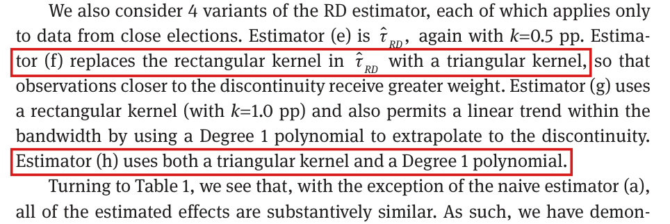
The sentences on p. 3 should read: “In fact, under Conditions 1–3 of Proposition 1, the OLS estimate from all elections equals the degree-0, rectangular-kernel RD estimate and relies solely on outcomes from close elections. When equation (2) exactly specifies the conditional mean, under conditions giving shared consistency, the polynomial OLS and shrinking-bandwidth RD estimates converge to the same cutoff jump and their difference converges to zero in probability. Outcomes of elections outside the close-election window can also enter the polynomial OLS estimate.”
The sentence on p. 7 should read: “The OLS estimator with the coarsened control of Proposition 1 uses outcomes from close elections only. An exactly specified polynomial regression can also use distant outcomes. Under shared consistency, its difference from a shrinking-bandwidth RD estimate converges to zero in probability; this does not imply equal observation weights, sampling variance or finite-sample bias.”
The second sentence of Section 5, p. 8, should read: “The limitations of studying close elections apply in full to the coarsened regression. For a polynomial regression, concerns about causal interpretation and scope can be shared when they arise from the common cutoff target and the same identifying assumptions; equal targets alone do not imply equal bias.”









My comment and the history of this entry
Suggested classification: clarity note.
My position My comment above; I suggested a clarity note.
The models’ position Under its natural reading, the claim that polynomial regression uses only close-election outcomes is false and can mislead readers about which data the estimate depends on, although the equivalence results, the reported estimates and the shared causal concerns survive: Moderate.