LLM-generated corrections to the published research of P. M. Aronow

Journal article P028

Corrections to: Sharp Bounds for Complier Average Potential Outcomes in Experiments with Noncompliance and Incomplete Reporting

P. M. Aronow and Donald P. Green (2013). Sharp Bounds for Complier Average Potential Outcomes in Experiments with Noncompliance and Incomplete Reporting. Statistics and Probability Letters 83(3):677–679.

DOI
10.1016/j.spl.2012.11.012
Audited edition
Statistics and Probability Letters, 2013, 83(3):677–679; 3 pages in the audited file
SHA-256 of the audited file
c69f86414e9ff27e081e7dc841b732e15abf65dc185c889a33e97dd20789aa50
Permanent address
https://pmaronow.github.io/llm-audit/works/P028/

Summary

This letter asks what the usual published summaries of an experiment with noncompliance reveal about compliers. From the outcome mean in each assignment arm and the difference in take-up, it derives sharp bounds on the complier average potential outcomes (Proposition 1) and illustrates them with a debate-viewing experiment. 4 entries are classified as errors (4 Minor), and 2 are clarity notes. The most important error is that the example’s point estimates, 0.430.43 and 0.720.72, need an unstated assumption about 71 missing outcomes.

What was and was not checked

I checked the following statements, which held up within the qualifications below.

  • The LATE display of Section 2. Under (i)–(iv), E[D∣Z=1]−E[D∣Z=0]=Pc\mathrm{E}[D \mid Z = 1] - \mathrm{E}[D \mid Z = 0] = P_c, and (EY1−EY0)/Pc(EY_1 - EY_0)/P_c equals the CACE. This follows from the decomposition into always-takers, never-takers and compliers, and it holds exactly in finite models generated at random.
  • Equations (1), (2) and (3) and the three displayed inequalities in the proof of Proposition 1, for 0<Pc<10 < P_c < 1. The misprints are confined to the sentence between (3) and the display (see P028-E001), and the proof omits the case Pc=1P_c = 1 (see P028-E002).
  • Both intervals of Proposition 1, as printed. I rederived them by hand. They agree exactly with the set of feasible values in 4000 finite models generated at random, on a grid of 24,167 rational points, and for 6160 compatible triples (EY0,EY1,Pc)(EY_0, EY_1, P_c), some with Pc=1P_c = 1.
  • The sharpness of Proposition 1. Each endpoint, and each interior point that was tried, is attained by an explicit model that reproduces (EY0,EY1,Pc)(EY_0, EY_1, P_c) and in which compliers and never-takers have constant outcomes.
  • The remark after Proposition 1 on when the bounds are narrow. With τ=(EY1−EY0)/Pc\tau = (EY_1 - EY_0)/P_c, the width of each interval is the minimum of 11, 1−∣τ∣1 - |\tau|, EY0/PcEY_0/P_c, EY1/PcEY_1/P_c, (1−EY0)/Pc(1 - EY_0)/P_c, (1−EY1)/Pc(1 - EY_1)/P_c and (1−Pc)/Pc(1 - P_c)/P_c, and items (i), (ii) and (iii) of the remark correspond to these terms.
  • Corollary 1, under its premise that the four cell means exist. Its weighted-subtraction formula holds exactly in 4000 finite models generated at random, with zero-probability cell contributions set to zero for empty cells. The ratio defining E[Y∣D(1)=D(0)]\mathrm{E}[Y \mid D(1) = D(0)] in its proof requires Pc<1P_c < 1 (see P028-E002).
  • Section 4, first paragraph. The reported 0.450.45, 0.510.51 and 0.210.21 give 0.06/0.21≈0.2860.06/0.21 \approx 0.286, printed as 29 percentage points, and the intervals [0,5/7][0, 5/7] and [2/7,1][2/7, 1], printed as [0,0.71][0, 0.71] and [0.29,1][0.29, 1]. The source chapter reports the difference of 21 points in viewing, the outcome means 0.510.51 and 0.450.45, and the effect of 29 points (its p. 333 and Tables 12.1 and 12.4).
  • Section 4, second paragraph. The four quantities taken from the replication data are reproduced: 80/492≈0.16380/492 \approx 0.163, when three control respondents whose viewing answer was unsure or refused are left out, 320/505≈0.634320/505 \approx 0.634, 40/79≈0.50640/79 \approx 0.506 and 130/294≈0.442130/294 \approx 0.442. The outcome means among respondents whose outcome is recorded are 207/458≈0.452207/458 \approx 0.452 and 240/471≈0.510240/471 \approx 0.510, in agreement with the printed 0.450.45 and 0.510.51.
  • The description of the design in Section 4. The survey instrument and the data agree with it. Respondents were randomly assigned to be asked to watch the debate, and the control group was asked to watch another programme. The treatment DD is self-reported viewing, and the outcome YY is a change of opinion about at least one of the two candidates. Noncompliance is two-sided, since 80 of the 495 controls watched and 320 of the 505 encouraged respondents did not.
  • The recommendation of Section 5. The quantities E[Y∣D=d,Z=z]\mathrm{E}[Y \mid D = d, Z = z] and Pr⁡[D=d∣Z=z]\Pr[D = d \mid Z = z] determine EY0EY_0, EY1EY_1, PcP_c and the formula of Corollary 1. For a binary outcome they also determine the joint distribution of YY and DD given ZZ.
  • The cross-references. Each reference to a numbered equation, proposition or corollary points to the right item. The letter has no tables or figures.

I could not obtain the file with the list and coding of the 20 get-out-the-vote studies (footnote 1), so I could not check the count of 6 of 20 in Section 1. No analysis script for Section 4 is available. I reproduced 0.430.43 and 0.720.72 to rounding using the reported outcome means and the unrounded take-up rates and cell means from the data, with an inferred sample and first stage (see P028-N007). The replication files are the data and Stata code of the source study. Only the 2019 edition of those data, in which age is top-coded, was available. The exclusion restriction is assumed in the example and was not tested. The entries for Angrist, Imbens and Rubin (1996) and for Angrist and Pischke (2009) were not compared with those publications, and the body of Imbens and Rubin (1997) was not read. The letter has no simulations. A statement that has no correction here has not been shown to be correct.

Headline claims and related corrections

  1. Given only EY1=E[Y∣Z=1]EY_1 = \mathrm{E}[Y \mid Z = 1], EY0=E[Y∣Z=0]EY_0 = \mathrm{E}[Y \mid Z = 0] and PcP_c (the difference in take-up), with outcomes in [0,1][0,1], the complier average potential outcomes lie in the two closed intervals of Proposition 1, and these bounds are sharp.

    Abstract; Section 1, last paragraph; Proposition 1 and its proof, Eqs. (1)-(3)

    See P028-E001, P028-E002, P028-N002.

  2. Under random assignment, exclusion, a nonzero first stage and monotonicity, the two assignment-arm outcome means and the take-up difference suffice to estimate the CACE, (EY1−EY0)/Pc(EY_1 - EY_0)/P_c, but do not in general identify the two complier average potential outcomes.

    Section 1, first paragraph; Section 2 LATE display; Proposition 1

    See P028-N002.

  3. If E[Y∣D=d,Z=z]\mathrm{E}[Y \mid D = d, Z = z] and Pr⁡[D=d∣Z=z]\Pr[D = d \mid Z = z] are known for d,z∈{0,1}d,z \in \{0,1\}, the complier average potential outcomes are point identified by the formula of Corollary 1.

    Section 1, last sentence; Corollary 1 and its proof; Eqs. (1)-(2); Section 5

    See P028-E002, P028-E003.

  4. Published reports often omit the information needed to recover complier average potential outcomes: only 6 of the 20 published randomized get-out-the-vote canvassing studies collected for the paper report enough.

    Abstract ('often fail to report'); Section 1, second paragraph; footnote 1 (meta.csv)

  5. In the Mullainathan et al. debate experiment the published figures (EY0=0.45EY_0 = 0.45, EY1=0.51EY_1 = 0.51, Pc=0.21P_c = 0.21) give a CACE of 29 percentage points but only wide bounds: E[Y(0)∣D(1)>D(0)]∈[0,0.71]\mathrm{E}[Y(0) \mid D(1) > D(0)] \in [0,0.71] and E[Y(1)∣D(1)>D(0)]∈[0.29,1]\mathrm{E}[Y(1) \mid D(1) > D(0)] \in [0.29,1].

    Section 1, last paragraph; Section 4, first paragraph; Proposition 1 (no table or figure)

    See P028-N005, P028-N007.

  6. With four further quantities taken from the replication data, Corollary 1 gives point estimates E[Y(0)∣D(1)>D(0)]=0.43\mathrm{E}[Y(0) \mid D(1) > D(0)] = 0.43 and E[Y(1)∣D(1)>D(0)]=0.72\mathrm{E}[Y(1) \mid D(1) > D(0)] = 0.72, a considerable tightening relative to the bounds.

    Section 4, second paragraph; Corollary 1 (no table or figure)

    See P028-N005, P028-N007.

  7. Researchers should report estimates of E[Y∣D=d,Z=z]\mathrm{E}[Y \mid D = d, Z = z] and Pr⁡[D=d∣Z=z]\Pr[D = d \mid Z = z] for d,z∈{0,1}d,z \in \{0,1\}, so that complier average potential outcomes can be estimated from published results; for binary outcomes such reporting also facilitates alternative parametric models and robust variance estimators.

    Section 1, last sentence; Section 5; Corollary 1

Sources that could not be obtained

  • meta.csv, the coding sheet for the paper's survey of 20 studies (footnote 1, http://pantheon.yale.edu/~pma5/meta.csv)

Corrections

Minor (4)

Real but inconsequential, for example a misprint that does not change a result.

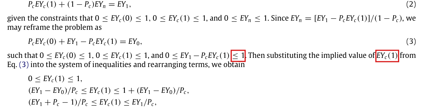
In the proof of Proposition 1, the third constraint after equation (3) has upper limit 1−Pc1 - P_c and not 11, and the mean substituted out of equation (3) is EYc(0)EY_c(0) and not EYc(1)EY_c(1); the three displayed inequalities and the proposition are unchanged.

Proof of Proposition 1, the sentence between equation (3) and the three displayed inequalities, p. 678 (PDF p. 2)

See also under Formal statements (Lean): P028-T4, P028-T5, P028-T8

As printed

Since EYn=[EY1−PcEYc(1)]/(1−Pc)EY_n = [EY_1 - P_c EY_c(1)]/(1 - P_c), we may reframe the problem as

PcEYc(0)+EY1−PcEYc(1)=EY0,(3)P_c EY_c(0) + EY_1 - P_c EY_c(1) = EY_0, \qquad (3)

such that 0≤EYc(0)≤10 \le EY_c(0) \le 1, 0≤EYc(1)≤10 \le EY_c(1) \le 1, and 0≤EY1−PcEYc(1)≤10 \le EY_1 - P_c EY_c(1) \le \colorbox{#ffe58a}{$1$}. Then substituting the implied value of EYc(1)\colorbox{#ffe58a}{$EY_c(1)$} from Eq. (3) into the system of inequalities and rearranging terms, we obtain

0≤EYc(1)≤1,(EY1−EY0)/Pc≤EYc(1)≤1+(EY1−EY0)/Pc,(EY1+Pc−1)/Pc≤EYc(1)≤EY1/Pc,\begin{aligned} &0 \le EY_c(1) \le 1,\\ &(EY_1 - EY_0)/P_c \le EY_c(1) \le 1 + (EY_1 - EY_0)/P_c,\\ &(EY_1 + P_c - 1)/P_c \le EY_c(1) \le EY_1/P_c, \end{aligned}

which yields the interval for EYc(1)EY_c(1) asserted by the proposition. The interval for EYc(0)EY_c(0) follows via substitution from the equality in Eq. (3).

The problem

The third constraint restates 0≤EYn≤10 \le EY_n \le 1 after the substitution EYn=[EY1−PcEYc(1)]/(1−Pc)EY_n = [EY_1 - P_c EY_c(1)]/(1 - P_c). Multiplying by 1−Pc1 - P_c, I obtain the upper limit 1−Pc1 - P_c, and the sentence prints 11. For 0<Pc<10 < P_c < 1 the printed constraint is weaker than the one it replaces. It implies only the lower bound (EY1−1)/Pc(EY_1 - 1)/P_c for EYc(1)EY_c(1), and not the lower bound (EY1+Pc−1)/Pc(EY_1 + P_c - 1)/P_c in the third line of the display. The next sentence names the wrong mean. Since the system that follows is written in EYc(1)EY_c(1), the mean eliminated through equation (3) is EYc(0)EY_c(0). The display itself uses the intended constraint and the intended substitution.

Evidence a derivation

I give a derivation, with an exact example which shows that the printed system is not equivalent to the original one. Suppose that 0<Pc<10 < P_c < 1. By (2), I have EYn=[EY1−PcEYc(1)]/(1−Pc)EY_n = [EY_1 - P_c EY_c(1)]/(1 - P_c), and therefore

0≤EYn≤1  ⟺  0≤EY1−PcEYc(1)≤1−Pc  ⟺  EY1+Pc−1Pc≤EYc(1)≤EY1Pc.0 \le EY_n \le 1 \iff 0 \le EY_1 - P_c EY_c(1) \le 1 - P_c \iff \frac{EY_1 + P_c - 1}{P_c} \le EY_c(1) \le \frac{EY_1}{P_c}.

By (3), I have EYc(0)=EYc(1)−(EY1−EY0)/PcEY_c(0) = EY_c(1) - (EY_1 - EY_0)/P_c, which implies that

0≤EYc(0)≤1  ⟺  EY1−EY0Pc≤EYc(1)≤1+EY1−EY0Pc.0 \le EY_c(0) \le 1 \iff \frac{EY_1 - EY_0}{P_c} \le EY_c(1) \le 1 + \frac{EY_1 - EY_0}{P_c}.

Together with 0≤EYc(1)≤10 \le EY_c(1) \le 1, these are the three displayed inequalities. Since (EY1+Pc−1)/Pc=1−(1−EY1)/Pc(EY_1 + P_c - 1)/P_c = 1 - (1 - EY_1)/P_c, their intersection is the interval for EYc(1)EY_c(1) in Proposition 1.

For the example, let Pc=1/2P_c = 1/2, EY0=EY1=3/4EY_0 = EY_1 = 3/4 and EYc(0)=EYc(1)=0EY_c(0) = EY_c(1) = 0. Equation (3) and the three printed constraints hold, since EY1−PcEYc(1)=3/4≤1EY_1 - P_c EY_c(1) = 3/4 \le 1. But the implied noncomplier mean is EYn=(3/4)/(1/2)=3/2>1EY_n = (3/4)/(1/2) = 3/2 > 1. For these values of PcP_c, EY0EY_0 and EY1EY_1, I obtain the interval [0,1][0, 1] for EYc(1)EY_c(1) from the printed system, and the interval [1/2,1][1/2, 1] of Proposition 1 from the corrected system.

What survives

Proposition 1, its sharpness, the three displayed inequalities and the LATE identity are unaffected. The bounds of the application are also unaffected. From the reported 0.450.45, 0.510.51 and 0.210.21 the intervals are [0,5/7][0, 5/7] and [2/7,1][2/7, 1], printed as [0,0.71][0, 0.71] and [0.29,1][0.29, 1]. The correction changes one limit and one symbol in the proof and has no cost. The case Pc=1P_c = 1 is treated in P028-E002.

Corrected

Since EYn=[EY1−PcEYc(1)]/(1−Pc)EY_n = [EY_1 - P_c EY_c(1)]/(1 - P_c), we may reframe the problem as

PcEYc(0)+EY1−PcEYc(1)=EY0,(3)P_c EY_c(0) + EY_1 - P_c EY_c(1) = EY_0, \qquad (3)

such that 0≤EYc(0)≤10 \le EY_c(0) \le 1, 0≤EYc(1)≤10 \le EY_c(1) \le 1, and 0≤EY1−PcEYc(1)≤1−Pc0 \le EY_1 - P_c EY_c(1) \le \colorbox{#ffe58a}{$1 - P_c$}. Then substituting the implied value of EYc(0)\colorbox{#ffe58a}{$EY_c(0)$} from Eq. (3) into the system of inequalities and rearranging terms, we obtain

0≤EYc(1)≤1,(EY1−EY0)/Pc≤EYc(1)≤1+(EY1−EY0)/Pc,(EY1+Pc−1)/Pc≤EYc(1)≤EY1/Pc,\begin{aligned} &0 \le EY_c(1) \le 1,\\ &(EY_1 - EY_0)/P_c \le EY_c(1) \le 1 + (EY_1 - EY_0)/P_c,\\ &(EY_1 + P_c - 1)/P_c \le EY_c(1) \le EY_1/P_c, \end{aligned}

which yields the interval for EYc(1)EY_c(1) asserted by the proposition. The interval for EYc(0)EY_c(0) follows via substitution from the equality in Eq. (3).

Crop of the proof of Proposition 1 from equation (2) through equation (3) to the three displayed inequalities. Red outlines surround two items in the sentence after equation (3). The first is the final less-than-or-equal-to 1 in the constraint 0 is at most EY sub 1 minus P sub c EY sub c (1), which is at most 1. The second is the symbol EY sub c (1) in the words: Then substituting the implied value of EY sub c (1) from Eq. (3). The third displayed inequality below begins (EY sub 1 + P sub c minus 1) / P sub c.
Proof of Proposition 1, p. 678 (PDF p. 2), from equation (2) to the three displayed inequalities. The outlines mark the upper limit 11 of the third constraint and the symbol EYc(1)EY_c(1) in “the implied value of EYc(1)EY_c(1)”.

Since the proof of Proposition 1 defines a mean among noncompliers and divides by 1−Pc1 - P_c, it needs a separate case for full compliance, Pc=1P_c = 1, which the assumptions allow; the printed intervals are correct in that case.

Proof of Proposition 1, first sentence and the sentence after equation (2), p. 678 (PDF p. 2); assumptions (iii) and (iv), Section 2, p. 678

See also under Formal statements (Lean): P028-T6, P028-T7, P028-T8, P028-T9

As printed

Section 2, p. 678. (iii) non-zero first-stage effect: E[Di(1)−Di(0)]≠0E[D_i(1) - D_i(0)] \neq 0; (iv) monotonicity: ∀i\forall i, Di(1)≥Di(0)D_i(1) \geq D_i(0).

Proof of Proposition 1, p. 678. Define EYn≡E[Y∣D(1)=D(0)]\colorbox{#ffe58a}{$EY_n \equiv \mathrm{E}[Y \mid D(1) = D(0)]$}, EYc(0)≡E[Y(0)∣D(1)>D(0)]EY_c(0) \equiv \mathrm{E}[Y(0) \mid D(1) > D(0)] and EYc(1)≡E[Y(1)∣D(1)>D(0)]EY_c(1) \equiv \mathrm{E}[Y(1) \mid D(1) > D(0)]. By the law of total probability,

PcEYc(0)+(1−Pc)EYn=EY0,(1)PcEYc(1)+(1−Pc)EYn=EY1,(2)\begin{aligned} P_c EY_c(0) + (1 - P_c) EY_n &= EY_0, \qquad (1)\\ P_c EY_c(1) + (1 - P_c) EY_n &= EY_1, \qquad (2) \end{aligned}

given the constraints that 0≤EYc(0)≤10 \le EY_c(0) \le 1, 0≤EYc(1)≤10 \le EY_c(1) \le 1, and 0≤EYn≤10 \le EY_n \le 1. Since EYn=[EY1−PcEYc(1)]/(1−Pc)EY_n = [EY_1 - P_c EY_c(1)]\colorbox{#ffe58a}{$/(1 - P_c)$}, we may reframe the problem as

The problem

Assumptions (iii) and (iv) imply that 0<Pc≤10 < P_c \le 1, and no assumption of Section 2 excludes Pc=1P_c = 1. When Pc=1P_c = 1 the event D(1)=D(0)D(1) = D(0) has probability zero. The mean EYnEY_n is then not defined, and the quotient [EY1−PcEYc(1)]/(1−Pc)[EY_1 - P_c EY_c(1)]/(1 - P_c) is 0/00/0. The proof treats no separate case and does not cover full compliance. The omission is in the proof and not in the result. At Pc=1P_c = 1 the two printed intervals reduce to the points EY0EY_0 and EY1EY_1, which are the complier average potential outcomes in that case. The ratio in the proof of Corollary 1 has the same denominator, Pr⁡[D=1∣Z=0]+Pr⁡[D=0∣Z=1]=1−Pc\Pr[D = 1 \mid Z = 0] + \Pr[D = 0 \mid Z = 1] = 1 - P_c. Corollary 1 assumes that the four cell means E[Y∣D=d,Z=z]\mathrm{E}[Y \mid D = d, Z = z] are known. This assumption requires that Pc<1P_c < 1, and the corollary is correct as printed.

Evidence an exact counterexample

I give an exact counterexample to the step of the proof, together with a derivation that covers Pc=1P_c = 1. For the counterexample, let ZZ be 00 or 11 with probability 1/21/2 each, and suppose that D(0)=0D(0) = 0, D(1)=1D(1) = 1, Y(0)=0Y(0) = 0, Y(1)=1Y(1) = 1 and Y(d,z)=Y(d)Y(d, z) = Y(d) for every unit. Assumptions (i)–(iv) hold and Y∈[0,1]Y \in [0,1]. I have Pc=1P_c = 1, EY0=0EY_0 = 0, EY1=1EY_1 = 1, EYc(0)=0EY_c(0) = 0 and EYc(1)=1EY_c(1) = 1. However, Pr⁡[D(1)=D(0)]=0\Pr[D(1) = D(0)] = 0, and [EY1−PcEYc(1)]/(1−Pc)=0/0[EY_1 - P_c EY_c(1)]/(1 - P_c) = 0/0.

For the derivation, write p=Pcp = P_c, ez=EYze_z = EY_z and cd=EYc(d)c_d = EY_c(d), and let AA and NN denote the events D(0)=D(1)=1D(0) = D(1) = 1 (always-takers) and D(0)=D(1)=0D(0) = D(1) = 0 (never-takers). By monotonicity, Pr⁡(A)+Pr⁡(N)=1−p\Pr(A) + \Pr(N) = 1 - p. Define m=E[1AY(1)]+E[1NY(0)]m = \mathrm{E}[\mathbf{1}_A Y(1)] + \mathrm{E}[\mathbf{1}_N Y(0)]. Since Y∈[0,1]Y \in [0,1], I have 0≤m≤1−p0 \le m \le 1 - p. In the arm Z=0Z = 0 the observed outcome is Y(0)Y(0) for compliers and never-takers and Y(1)Y(1) for always-takers, and in the arm Z=1Z = 1 it is Y(1)Y(1) for compliers and always-takers and Y(0)Y(0) for never-takers. By random assignment and exclusion, it follows that

e0=p c0+m,e1=p c1+m.e_0 = p\,c_0 + m, \qquad e_1 = p\,c_1 + m .

These equations use no mean over the noncompliers. If p<1p < 1, then m=(1−p)EYnm = (1 - p) EY_n and they are (1) and (2). If p=1p = 1, then m=0m = 0, and I have c0=e0c_0 = e_0 and c1=e1c_1 = e_1. Setting Pc=1P_c = 1 in the printed intervals, I obtain

max⁡{0, e0−e1, e0}=e0=min⁡{1, 1−e1+e0, e0},max⁡{0, e1−e0, e1}=e1=min⁡{1, 1+e1−e0, e1},\begin{aligned} \max\{0,\, e_0 - e_1,\, e_0\} &= e_0 = \min\{1,\, 1 - e_1 + e_0,\, e_0\},\\ \max\{0,\, e_1 - e_0,\, e_1\} &= e_1 = \min\{1,\, 1 + e_1 - e_0,\, e_1\}, \end{aligned}

because 0≤e0≤10 \le e_0 \le 1 and 0≤e1≤10 \le e_1 \le 1. The two intervals are the points e0e_0 and e1e_1. In the arm Z=0Z = 0 the product Y⋅DY \cdot D equals Y(1)Y(1) on AA and 00 elsewhere, and in the arm Z=1Z = 1 the product Y⋅(1−D)Y \cdot (1 - D) equals Y(0)Y(0) on NN and 00 elsewhere. This implies the expression for mm in terms of observed variables that is used below. A check in exact arithmetic agrees. The printed intervals are single points in 81 models with full compliance, and the formulas with mm hold in 810 finite models, some with empty cells.

What survives

The intervals of Proposition 1 are correct as printed, for Pc=1P_c = 1 as well as for Pc<1P_c < 1, and they remain sharp. The LATE identity divides by Pc>0P_c > 0 and is unaffected, and Corollary 1 holds under its premise that the four cell means are known. The application has two-sided noncompliance, with Pc=0.21P_c = 0.21, and no printed number changes. The repair adds a case to the proof and no assumption.

Corrected

Insert at the start of the proof of Proposition 1:

If Pc=1P_c = 1, a unit is a complier with probability one, so EYc(0)=EY0EY_c(0) = EY_0 and EYc(1)=EY1EY_c(1) = EY_1; the displayed intervals reduce to these singletons. Henceforth suppose 0<Pc<10 < P_c < 1.

The proof can also be written with no mean over the noncompliers, and then no separate case is needed. Assume (i)–(iv) of Section 2 and Y∈[0,1]Y \in [0,1], and assume that both assignment arms have positive probability. Let CC denote the complier event D(1)>D(0)D(1) > D(0), and set p=Pc=Pr⁡(C)>0p = P_c = \Pr(C) > 0, ez=EYz=E[Y∣Z=z]e_z = EY_z = \mathrm{E}[Y \mid Z = z] and cd=E[Y(d)∣C]c_d = \mathrm{E}[Y(d) \mid C]. Define the noncomplier contribution

m=E[Y⋅D∣Z=0]+E[Y⋅(1−D)∣Z=1],m = \mathrm{E}[Y \cdot D \mid Z = 0] + \mathrm{E}[Y \cdot (1 - D) \mid Z = 1],

where YY and DD are the observed outcome and treatment and the dot denotes multiplication. Then

0≤m≤1−p,ez=p cz+mfor z∈{0,1}.0 \le m \le 1 - p, \qquad e_z = p\,c_z + m \quad \text{for } z \in \{0, 1\}.

For p<1p < 1, m=(1−p)EYnm = (1 - p) EY_n. For p=1p = 1, m=0m = 0 and cz=ezc_z = e_z, with no mean over an empty group and no division by 1−p1 - p.

Corollary 1 is correct as printed when the four cell means exist. To state it in a form that allows empty treatment-by-assignment cells, replace its two weighted cell means by the two product moments in mm, and use c0=(e0−m)/pc_0 = (e_0 - m)/p and c1=(e1−m)/pc_1 = (e_1 - m)/p. Each product moment equals the printed probability times the cell mean whenever that cell mean exists, and it is zero when the cell is empty.

Crop of the first six lines of the proof of Proposition 1, with equations (1) and (2). Red outlines surround two items. The first is the definition EY sub n is identically E of Y given D(1) = D(0), in the first line of the proof. The second is the divisor, slash open parenthesis 1 minus P sub c close parenthesis, in the sentence: Since EY sub n = [EY sub 1 minus P sub c EY sub c (1)] / (1 minus P sub c), we may reframe the problem as.
Proof of Proposition 1, p. 678 (PDF p. 2). The outlines mark the definition of the noncomplier mean EYnEY_n and the division by 1−Pc1 - P_c.

The Imbens and Rubin (1997) entry prints the issue number, 4, where the volume belongs; the article is in Review of Economic Studies, volume 64, issue 4, pp. 555–574.

References, third entry (Imbens and Rubin, 1997), p. 679 (PDF p. 3)

As printed

Imbens, G.W., Rubin, D.B., 1997. Estimating outcome distributions for compliers in instrumental variables models. Review of Economic Studies 4, 555–574.

The problem

The numeral 4 stands where the other journal entry of the list has its volume (“Journal of the American Statistical Association 91, 444–455”). The article is in volume 64, and 4 is the number of the issue. The entry omits the volume.

Evidence a check of the printed page

I checked the journal’s table of contents. Oxford Academic lists the article under “The Review of Economic Studies, Volume 64, Issue 4, October 1997, Pages 555–574”.

What survives

The cited work is identified by its authors, title, year and pages, and no result of the paper depends on the entry.

Corrected

Imbens, G.W., Rubin, D.B., 1997. Estimating outcome distributions for compliers in instrumental variables models. Review of Economic Studies 64, 555–574.

Crop of the four entries of the reference list. A red outline surrounds the numeral 4 in the third entry, which ends: Review of Economic Studies 4, 555 to 574. The first entry ends: Journal of the American Statistical Association 91, 444 to 455.
References, p. 679 (PDF p. 3). The outline marks the numeral 4 in the Imbens and Rubin (1997) entry, in the position where the first entry gives the volume 91.

The point estimates 0.430.43 and 0.720.72 require an assumption about the 71 respondents whose outcome is missing, and the paper states none; under the assumptions of Section 2 alone, the replication data do not point identify the complier average potential outcomes.

Section 4, second paragraph, p. 679 (PDF p. 3)

See also under Formal statements (Lean): P028-T1, P028-T2, P028-T3

As printed

Point identification is possible when additional information about the joint distribution of Y,D,ZY, D, Z is known. Since the replication data set is publicly available for the study2^{2}, we are able to fill in the necessary missing information: Pr⁡[D=1∣Z=0]=0.163\Pr[D = 1 \mid Z = 0] = 0.163, Pr⁡[D=0∣Z=1]=0.634\Pr[D = 0 \mid Z = 1] = 0.634, E[Y∣D=1,Z=0]=0.506\mathrm{E}[Y \mid D = 1, Z = 0] = 0.506 and E[Y∣D=0,Z=1]=0.442\mathrm{E}[Y \mid D = 0, Z = 1] = 0.442. Application of Corollary 1 yields E[Y(0)∣D(1)>D(0)]=0.43\mathrm{E}[Y(0) \mid D(1) > D(0)] = 0.43 and E[Y(1)∣D(1)>D(0)]=0.72\mathrm{E}[Y(1) \mid D(1) > D(0)] = 0.72.

The problem

The source study codes the outcome as 11 if the respondent’s opinion of either mayoral candidate changed, as 00 if both opinions were unchanged, and as missing otherwise. With this coding the outcome is missing for 71 of the 1000 respondents in the replication data: 37 of the 495 assigned to control and 34 of the 505 assigned to encouragement, at different rates in the four cells defined by assignment and viewing. The paper does not mention these respondents. It does not say which respondents enter each quantity, and it states no assumption about nonresponse. Section 2 assumes random assignment, exclusion, a non-zero first stage, monotonicity and bounded outcomes, and none of these assumptions concerns which outcomes are recorded. Corollary 1 identifies the two complier average potential outcomes, which I call the complier means, from the joint distribution of (Y,D,Z)(Y, D, Z) in the study population. The replication data determine the distribution of YY only among respondents whose outcome is recorded, and a mean among those respondents equals the corresponding population mean only under a further assumption. The words “we are able to fill in the necessary missing information” claim more than the data supply. The values 0.430.43 and 0.720.72 are presented as point estimates under the assumptions of Section 2, and they also depend on an assumption about nonresponse that the paper does not state and that random assignment does not imply.

The correction does not say that either number is wrong. Under conventional treatments of the missing outcomes the estimates are about 0.440.44 and 0.720.72, and no bias is shown. The repair has a cost. To keep 0.430.43 and 0.720.72 as point estimates for the study population, one must add an assumption about nonresponse that the application may not satisfy. Without such an assumption, the point estimates must be replaced by a range over the missing outcomes, which is a weaker conclusion.

Evidence an exact counterexample

The evidence is an exact counterexample. There exist two models that satisfy every assumption of Section 2, in which the observed data have the same distribution and the complier means differ. The observed data are the assignment ZZ, the viewing variable DD as coded in the replication data, whether the outcome is recorded, and the outcome when it is recorded. The table lists the counts.

Respondents in the replication data, by assignment ZZ and viewing DD. The outcome YY is coded as in the source study.
ZZDDRespondentsOutcome recordedY=1Y = 1Y=0Y = 0Outcome missing
0041537916721236
01807940391
1032029413016426
11185177110678

Let xzdx_{zd} denote the number of missing outcomes in the cell (Z,D)=(z,d)(Z, D) = (z, d) that equal 11, so that 0≤x00≤360 \le x_{00} \le 36, 0≤x01≤10 \le x_{01} \le 1, 0≤x10≤260 \le x_{10} \le 26 and 0≤x11≤80 \le x_{11} \le 8. For the counterexample I treat the proportions within each arm, completed in this way, as a population distribution. Under monotonicity the cell (Z,D)=(0,1)(Z, D) = (0, 1) consists of always-takers and the cell (1,0)(1, 0) of never-takers. Their probabilities are pa=80/495p_a = 80/495 and pn=320/505p_n = 320/505, and compliers have probability pc=1−pa−pn=2047/9999p_c = 1 - p_a - p_n = 2047/9999. Let μd=E[Y(d)∣D(1)>D(0)]\mu_d = \mathrm{E}[Y(d) \mid D(1) > D(0)]. By random assignment and exclusion, I have

167+x00495=130+x10505+pc μ0,110+x11505=40+x01495+pc μ1.\frac{167 + x_{00}}{495} = \frac{130 + x_{10}}{505} + p_c\,\mu_0, \qquad \frac{110 + x_{11}}{505} = \frac{40 + x_{01}}{495} + p_c\,\mu_1 .

These are the equations of Corollary 1, written with joint probabilities. Solving them, I obtain

μ0=(167+x00)/495−(130+x10)/5052047/9999,μ1=(110+x11)/505−(40+x01)/4952047/9999.\mu_0 = \frac{(167 + x_{00})/495 - (130 + x_{10})/505}{2047/9999}, \qquad \mu_1 = \frac{(110 + x_{11})/505 - (40 + x_{01})/495}{2047/9999}.

Choosing (x00,x01,x10,x11)=(0,1,26,0)(x_{00}, x_{01}, x_{10}, x_{11}) = (0, 1, 26, 0), I obtain

(μ0,μ1)=(1423/10235, 6749/10235)≈(0.139, 0.659),(\mu_0, \mu_1) = (1423/10235,\ 6749/10235) \approx (0.139,\ 0.659),

and the choice (36,0,0,8)(36, 0, 0, 8) gives

(μ0,μ1)=(7633/10235, 7642/10235)≈(0.746, 0.747).(\mu_0, \mu_1) = (7633/10235,\ 7642/10235) \approx (0.746,\ 0.747).

Since μ0\mu_0 increases in x00x_{00} and decreases in x10x_{10}, and μ1\mu_1 increases in x11x_{11} and decreases in x01x_{01}, these are the extreme values over all completions of the missing outcomes.

For each of the two choices there exists an explicit population model. It has always-takers, never-takers and compliers with probabilities pap_a, pnp_n and pcp_c, binary potential outcomes, and, for each assignment, an indicator that the outcome is recorded whose probability depends on the type of the unit and on its outcome. In each model the assignment is independent of all potential variables, exclusion and monotonicity hold, the first stage is 2047/99992047/9999, and the observed data have the distribution in the table. A check in exact arithmetic verifies these properties for the two choices and for the other 14 choices such that each xzdx_{zd} is 00 or its maximum.

The ranges are extrema over the missing binary outcomes, with viewing held as coded. They are not confidence intervals, and they do not show that 0.430.43 or 0.720.72 is biased. Under three conventional treatments of the missing outcomes, the estimates are close to the printed ones. With outcome means among respondents whose outcome is recorded and take-up rates among all respondents, I obtain (0.439,0.721)(0.439, 0.721) from Corollary 1. With every quantity computed among the 929 respondents whose outcome is recorded, I find (0.436,0.719)(0.436, 0.719). With the cell means among recorded outcomes weighted by the cell probabilities among all respondents, the estimates are (0.436,0.712)(0.436, 0.712).

What survives

Corollary 1 is unaffected, since it identifies the complier means when the population moments in its statement are known. Proposition 1 and the reporting recommendation of Section 5 do not depend on the example, and no printed number is shown to be wrong. What changes is the status of 0.430.43 and 0.720.72, and of the statement that the replication data tighten inference to point estimates. Both hold only under an added assumption about nonresponse. The CACE of 29 percentage points and the bounds of the first paragraph use outcome means among respondents whose outcome is recorded. They need the same care if they are read as statements about the whole study population.

Corrected

Point identification is possible when additional information about the joint distribution of Y,D,ZY, D, Z is known. Since the replication data set is publicly available for the study2^{2}, we are able to estimate the necessary missing quantities: Pr⁡[D=1∣Z=0]=0.163\Pr[D = 1 \mid Z = 0] = 0.163, Pr⁡[D=0∣Z=1]=0.634\Pr[D = 0 \mid Z = 1] = 0.634, E[Y∣D=1,Z=0]=0.506\mathrm{E}[Y \mid D = 1, Z = 0] = 0.506 and E[Y∣D=0,Z=1]=0.442\mathrm{E}[Y \mid D = 0, Z = 1] = 0.442. The outcome is missing for 71 of the 1000 respondents, 37 of the 495 assigned to control and 34 of the 505 assigned to encouragement. Assume in addition that, within each assignment group, whether the outcome is recorded is independent of (Y,D)(Y, D), so that means among the respondents whose outcome is recorded estimate the corresponding population means. Under this assumption, the reported values can be interpreted as point estimates for the study population: E[Y(0)∣D(1)>D(0)]=0.43\mathrm{E}[Y(0) \mid D(1) > D(0)] = 0.43 and E[Y(1)∣D(1)>D(0)]=0.72\mathrm{E}[Y(1) \mid D(1) > D(0)] = 0.72. Without an assumption about the missing outcomes, these data do not point identify the complier average potential outcomes.

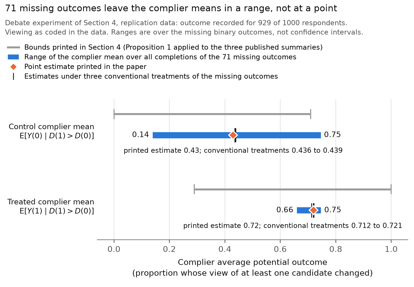
The added assumption is sufficient for a calculation that takes the outcome means from the respondents whose outcome is recorded and the take-up rates from all respondents. It does not follow from random assignment and does not specify the exact calculation of the printed values; I have not established it for this study. A complete statement would also give the coding of the outcome and of viewing and the respondents who enter each quantity; the paper’s own analysis script and original denominators are unavailable. If no assumption about nonresponse is made, the two point estimates should be replaced by the ranges over the missing outcomes: with viewing as coded in the replication data, 0.140.14 to 0.750.75 for the control complier mean and 0.660.66 to 0.750.75 for the treated complier mean.

Crop of the end of the first paragraph of Section 4, which gives the bounds [0, 0.71] and [0.29, 1], and of the whole second paragraph. A red outline surrounds the words: we are able to fill in the necessary missing information. The paragraph continues with the four quantities 0.163, 0.634, 0.506 and 0.442 and with the sentence: Application of Corollary 1 yields E[Y(0) | D(1) > D(0)] = 0.43 and E[Y(1) | D(1) > D(0)] = 0.72.
Section 4, second paragraph, p. 679 (PDF p. 3), with the last three lines of the first paragraph. The outline marks the words “we are able to fill in the necessary missing information”.
Chart with a horizontal axis from 0 to 1, labelled complier average potential outcome, the proportion whose view of at least one candidate changed. Title: 71 missing outcomes leave the complier means in a range, not at a point. There are two rows. In the row for the control complier mean, a grey line runs from 0 to 0.71, the bounds printed in Section 4, and below it a blue bar runs from 0.14 to 0.75, the range over all completions of the 71 missing outcomes. An orange diamond on the bar marks the printed estimate 0.43, and black ticks just to its right mark the estimates under three conventional treatments, 0.436 to 0.439. In the row for the treated complier mean, the grey line runs from 0.29 to 1 and the blue bar from 0.66 to 0.75, with the diamond at the printed estimate 0.72 and the ticks at 0.712 to 0.721.
The two complier means in the example of Section 4 when the 71 missing outcomes are unrestricted. For each mean the blue bar is the range over all completions of the missing binary outcomes, with viewing as coded in the replication data; the diamond is the point estimate printed in the paper; the black ticks are the estimates under three conventional treatments of the missing outcomes; and the grey line is the interval printed in the first paragraph of Section 4, shown for comparison. The ranges are not confidence intervals.

Clarity notes

Imprecise or ambiguous wording whose intended meaning is correct; not an error.

The unit index is dropped as a change to generic-unit population notation, in which DD and YY are the realized treatment and outcome; random assignment does not make the unit labels exchangeable, and no further assumption is needed.

Section 2, first paragraph, p. 678 (PDF p. 2)

As printed

We assume (i) random assignment: [Yi(d,z),Di(z):d,z∈{0,1}]⊥ ⁣ ⁣ ⁣⊥Zi[Y_i(d, z), D_i(z) : d, z \in \{0, 1\}] \perp\!\!\!\perp Z_i; (ii) exclusion restriction: Yi(d,z)Y_i(d, z) does not depend on zz, so we may write Yi(d,z)=Yi(d)Y_i(d, z) = Y_i(d); (iii) non-zero first-stage effect: E[Di(1)−Di(0)]≠0E[D_i(1) - D_i(0)] \neq 0; (iv) monotonicity: ∀i\forall i, Di(1)≥Di(0)D_i(1) \geq D_i(0). We make two notational simplifications. First, given (i), labels are exchangeable and so we drop notational dependence on ii. Second, we define Pc≡Pr⁡[D(1)>D(0)]P_c \equiv \Pr[D(1) > D(0)], EY1≡E[Y∣Z=1]EY_1 \equiv \mathrm{E}[Y \mid Z = 1], and EY0≡E[Y∣Z=0]EY_0 \equiv \mathrm{E}[Y \mid Z = 0].

Intended meaning

The sentence changes notation. From this point the paper writes Y(d)Y(d), D(z)D(z) and ZZ for a generic unit of the population, and D=D(Z)D = D(Z) and Y=Y(D)Y = Y(D) denote the realized treatment and the realized outcome. The paper does not display these two identities, but their usual meaning is clear from the definitions before the sentence, from the discussion of population quantities after it, and from the application. On this reading the LATE identity, Proposition 1 and Corollary 1 hold as stated.

Read literally, the reason given for dropping the index does not hold. Assumption (i) says that the assignment of each unit is independent of the potential outcomes and potential treatments of that unit, and this does not imply that the unit labels are exchangeable. For example, consider two units such that Di(0)=0D_i(0) = 0 and Di(1)=1D_i(1) = 1, with Y1(0)=Y1(1)=0Y_1(0) = Y_1(1) = 0 and Y2(0)=Y2(1)=1Y_2(0) = Y_2(1) = 1, each assigned by an independent fair coin. Since the potential outcomes of each unit are constant, (i) holds. However, the outcome of the first unit is always 00, and the outcome of the second is always 11.

The same example shows that the index can be dropped without assuming that the units are identically distributed. Let the generic unit be one of the two units, chosen with probability 1/21/2 each and independently of the assignments. By a direct computation, I find that E[Y∣Z=0]=E[Y∣Z=1]=1/2\mathrm{E}[Y \mid Z = 0] = \mathrm{E}[Y \mid Z = 1] = 1/2. The population quantities of Section 2 are defined in this example, although the two units have different outcome distributions.

Corrected

We make two notational simplifications. First, we drop notational dependence on ii and use generic-unit population notation, writing D=D(Z)D = D(Z) and Y=Y(D)Y = Y(D) for the realized treatment and outcome. Second, we define Pc≡Pr⁡[D(1)>D(0)]P_c \equiv \Pr[D(1) > D(0)], EY1≡E[Y∣Z=1]EY_1 \equiv \mathrm{E}[Y \mid Z = 1], and EY0≡E[Y∣Z=0]EY_0 \equiv \mathrm{E}[Y \mid Z = 0].

Crop of seven lines of Section 2, from the sentence that defines the treatment assigned to unit i through the four assumptions (i) to (iv) to the first two lines of the next paragraph. A red outline surrounds the words: given (i), labels are exchangeable. The sentence reads: First, given (i), labels are exchangeable and so we drop notational dependence on i.
Section 2, first paragraph, p. 678 (PDF p. 2). The outline marks the words “given (i), labels are exchangeable”, the reason given for dropping the unit index ii.

The seven figures printed in Section 4 are not one consistently rounded set, and the paper does not state the calculation behind 0.430.43 and 0.720.72; both values are reproduced when the reported outcome means are combined with unrounded take-up rates and cell means from the replication data.

Section 4, first and second paragraphs, p. 679 (PDF p. 3)

As printed

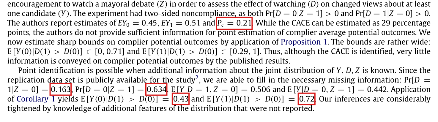
The authors report estimates of EY0=0.45EY_0 = 0.45, EY1=0.51EY_1 = 0.51 and Pc=0.21\colorbox{#ffe58a}{$P_c = 0.21$}. While the CACE can be estimated as 29 percentage points, the authors do not provide sufficient information for point estimation of complier average potential outcomes. […] Since the replication data set is publicly available for the study2^{2}, we are able to fill in the necessary missing information: Pr⁡[D=1∣Z=0]=0.163\Pr[D = 1 \mid Z = 0] = \colorbox{#ffe58a}{$0.163$}, Pr⁡[D=0∣Z=1]=0.634\Pr[D = 0 \mid Z = 1] = \colorbox{#ffe58a}{$0.634$}, E[Y∣D=1,Z=0]=0.506\mathrm{E}[Y \mid D = 1, Z = 0] = 0.506 and E[Y∣D=0,Z=1]=0.442\mathrm{E}[Y \mid D = 0, Z = 1] = 0.442. Application of Corollary 1 yields E[Y(0)∣D(1)>D(0)]=0.43\mathrm{E}[Y(0) \mid D(1) > D(0)] = \colorbox{#ffe58a}{$0.43$} and E[Y(1)∣D(1)>D(0)]=0.72\mathrm{E}[Y(1) \mid D(1) > D(0)] = \colorbox{#ffe58a}{$0.72$}. Our inferences are considerably tightened by knowledge of additional features of the distribution that were not reported.

Intended meaning

The first paragraph of Section 4 uses the three figures reported by the source study, and the second paragraph reports point estimates that were computed after consulting the replication data. All of these figures are rounded estimates, and on this reading the two paragraphs need not use the same first stage. The paper does not say which first stage and which precision enter the point estimates, and the printed figures alone do not reproduce them.

Under monotonicity, Pc=1−Pr⁡[D=1∣Z=0]−Pr⁡[D=0∣Z=1]P_c = 1 - \Pr[D = 1 \mid Z = 0] - \Pr[D = 0 \mid Z = 1]. Rates that round to 0.1630.163 and 0.6340.634 imply that 0.202<Pc≤0.2040.202 < P_c \le 0.204, while a first stage that rounds to 0.210.21 satisfies 0.205≤Pc<0.2150.205 \le P_c < 0.215. Hence the seven printed figures are not one consistently rounded set. Substituting them into Corollary 1, I obtain

0.45−0.163⋅0.506−0.634⋅0.4420.21=0.0872940.21≈0.4157,0.4157+0.51−0.450.21≈0.7014,\frac{0.45 - 0.163 \cdot 0.506 - 0.634 \cdot 0.442}{0.21} = \frac{0.087294}{0.21} \approx 0.4157, \qquad 0.4157 + \frac{0.51 - 0.45}{0.21} \approx 0.7014,

which round to 0.420.42 and 0.700.70. With Pc=0.203P_c = 0.203, the value implied by the two printed rates, the same substitution gives 0.43000.4300 and 0.72560.7256, which round to 0.430.43 and 0.730.73.

One calculation returns both printed values. I keep the reported outcome means 0.450.45 and 0.510.51, and I take from the replication data the unrounded take-up rates 80/49280/492 and 320/505320/505, the unrounded cell means 40/7940/79 and 130/294130/294, and the first stage Pc=1−80/492−320/505=2531/12423≈0.2037P_c = 1 - 80/492 - 320/505 = 2531/12423 \approx 0.2037. The rate 80/49280/492 leaves out three control respondents whose answer to the viewing question was “not sure” or a refusal. Using Corollary 1, I find

0.45−80492⋅4079−320505⋅1302942531/12423≈0.4294,0.51−80492⋅4079−320505⋅1302942531/12423≈0.7239,\begin{aligned} \frac{0.45 - \frac{80}{492} \cdot \frac{40}{79} - \frac{320}{505} \cdot \frac{130}{294}}{2531/12423} &\approx 0.4294,\\ \frac{0.51 - \frac{80}{492} \cdot \frac{40}{79} - \frac{320}{505} \cdot \frac{130}{294}}{2531/12423} &\approx 0.7239, \end{aligned}

which round to 0.430.43 and 0.720.72. No analysis script for the application is available. This calculation is a reconstruction and may differ from the one originally made.

With every input computed from the replication data at full precision, the estimates round to 0.440.44 and 0.720.72 under each of three conventions for the sample and for the coding of viewing: (0.4393,0.7207)(0.4393, 0.7207), (0.4390,0.7217)(0.4390, 0.7217) and (0.4359,0.7192)(0.4359, 0.7192). No printed estimate is shown to be wrong. The printed estimates lie inside the printed bounds [0,0.71][0, 0.71] and [0.29,1][0.29, 1], and this note does not affect the statement that the additional information tightens the inferences. The assumption on which the point estimates rest is the subject of P028-N005.

Corrected

Application of Corollary 1 yields E[Y(0)∣D(1)>D(0)]=0.43\mathrm{E}[Y(0) \mid D(1) > D(0)] = 0.43 and E[Y(1)∣D(1)>D(0)]=0.72\mathrm{E}[Y(1) \mid D(1) > D(0)] = 0.72. These point estimates can be reproduced by retaining the reported outcome means 0.450.45 and 0.510.51 and using the unrounded take-up rates and cell outcome means from the replication data. With uncertain viewing responses coded as missing, this calculation uses the first stage Pc=1−80/492−320/505≈0.204P_c = 1 - 80/492 - 320/505 \approx 0.204, rather than the 0.210.21 reported by the source study.

The added sentences describe one calculation that reproduces the printed values. If the original calculation was different, they should describe that calculation.

Crop of Section 4 from its second line to the end of its second paragraph. Red outlines surround five items. In the first paragraph: P sub c = 0.21, in the sentence The authors report estimates of EY sub 0 = 0.45, EY sub 1 = 0.51 and P sub c = 0.21. In the second paragraph: the values 0.163 and 0.634 of the two take-up rates, and the values 0.43 and 0.72 in the sentence Application of Corollary 1 yields E[Y(0) | D(1) > D(0)] = 0.43 and E[Y(1) | D(1) > D(0)] = 0.72.
Section 4, p. 679 (PDF p. 3). The outlines mark the first stage Pc=0.21P_c = 0.21 in the first paragraph, and the take-up rates 0.1630.163 and 0.6340.634 and the point estimates 0.430.43 and 0.720.72 in the second.

Formal statements (Lean)

Formal results: 9 whole; 0 restricted; 0 refuted; 1 omitted.

Coverage concerns the identified claim under its stated assumptions. A checked proof establishes the formal statement; correspondence to the published text was reviewed by AI. Repository access is currently required to open the source links.

Each result links to its current formal statement and proof. “Whole” covers the identified claim under its assumptions; “restricted” covers the stated narrower scope; “refuted” gives a counterexample to the identified assertion; “omitted” has no current theorem. Any named published theorem used as a premise remains an assumption. Browse the formal results for this work.

Section 4, second paragraph: ‘we are able to fill in the necessary missing information ... Application of Corollary 1 yields ...’, read as the claim that the replication data and the assumptions of Section 2 point identify the complier average potential outcomes; the two witnesses are the validator's constructions and are not in the paper

p. 679 (PDF p. 3), Section 4, second paragraph; the assumptions are on p. 678 (PDF p. 2), Section 2

Section 4, p. 679, with the Section 2 assumptions, p. 678. The two explicit seventeen-atom laws have the stated integer completions, positive completed counts, Bernoulli parameters, conditional product construction, stratum probabilities, source table, full and respondent moments, and different complier means. They satisfy random assignment including response potentials and have the same recorded-data law; neither complier mean is a real-valued function of that law in all admissible models. The usual measure-theoretic conditions are assumed.

Historical component credits
  • Counterexample proved AronowAudit.P028.missing_outcome_counterexample Historical support retained; baseline fidelity: ok; manifest: used; used in Solution; All standing assumptions hold for the concrete product laws: the atom type gives exclusion and binary bounds, finiteValid gives monotonicity and a positive first stage, and the other credited lemmas certify assignment and probability validity.
  • Proved AronowAudit.P028.finite_assignment_independent Historical support retained; baseline fidelity: ok; manifest: used; used in Solution; This is an algebraic supporting lemma, not a claim that an arbitrary BinaryLaw is a probability law. Positivity and normalization for the target witnesses are supplied by R185-05 and R185-08.
  • Proved AronowAudit.P028.missing_witness_assumptions Historical support retained; baseline fidelity: ok; manifest: used; used in Solution; finiteValid includes the first-stage identity as a conjunct, but the theorem verifies it for two fixed objects instead of assuming an identification result.
  • Proved AronowAudit.P028.missing_witness_observed_cells Historical support retained; baseline fidelity: ok; manifest: used; used in Solution; Products with the independent positive assignment coin turn the latent finite sums into the stated assignment-conditional probabilities.
  • Proved AronowAudit.P028.missing_witness_same_observed_law Historical support retained; baseline fidelity: ok; manifest: used; used in Solution; Its component is already included in the counterexample or product-law certificate used here; no separate helper conclusion is packaged.
  • Proved AronowAudit.P028.missing_witness_complier_means Historical support retained; baseline fidelity: ok; manifest: used; used in Solution; Its component is already included in the counterexample or product-law certificate used here; no separate helper conclusion is packaged.
  • Proved AronowAudit.P028.missing_outcome_not_identified Historical support retained; baseline fidelity: ok; manifest: used; used in Solution; Quantifying the negation over a subclass does not narrow a non-identification counterexample: any identifying functional for the full class would distinguish these two admissible laws. Rational versus real representation loses no witness cases.
  • Proved AronowAudit.P028.missing_witness_reported_moments Historical support retained; baseline fidelity: ok; manifest: used; used in Solution; The universal quantifier ranges only over the two specified witness laws, exactly as required by N2 and N4; this is not offered as a general missing-data identity.
  • Proved AronowAudit.P028.missing_witness_corollary_comparison Historical support retained; baseline fidelity: ok; manifest: used; used in Solution; The full-population calculation and the available-case plug-in calculation remain distinct. Together with R185-06 the equalities give precisely N4 and N5.
  • Proved AronowAudit.P028.finite_joint_normalized Historical support retained; baseline fidelity: ok; manifest: used; used in Solution; Its component is already included in the counterexample or product-law certificate used here; no separate helper conclusion is packaged.
  • Proved AronowAudit.P028.missing_witness_joint_probability Historical support retained; baseline fidelity: ok; manifest: used; used in Solution; The positive normalized rational array is an ordinary finite probability distribution; no additional Measure-valued construction is needed for this concrete witness.

Section 4, second paragraph, the inference from the replication data to the complier means 0.43 and 0.72, as repaired by Sol: identification of the complier average potential outcomes from incompletely recorded outcomes under a stated response condition

p. 679 (PDF p. 3), Section 4, second paragraph; Corollary 1 is on p. 678 (PDF p. 2)

Section 4, p. 679, repaired using Corollary 1, p. 678. Joint moments identify complier means without positive treatment cells. The stated mean equalities justify mixed respondent formulas; conditional response independence suffices. Cellwise mean ignorability justifies reweighting but need not justify the mixed formulas. With unrestricted response the stated bounds depend only on the recorded-data law. All source-table values and approximations hold; both endpoints of each source interval are attained, so no valid interval can be narrower. The usual measure-theoretic conditions are assumed.

Historical component credits
  • Proved AronowAudit.P028.response_joint_moment_identity Historical support retained; baseline fidelity: ok; manifest: used; used in Solution; These are exactly clause (i)'s identities: Boolean treatment indicators equal D or 1-D, and no positive treatment-assignment cell is required. The identities alone do not assert that the unrecorded full outcome moments are observed. The record also recognizes the boundedness generalization, but labels it faithful_with_notes rather than broader_than_claim.
  • Proved AronowAudit.P028.missing_moment_difference_bounds Historical support retained; baseline fidelity: ok; manifest: used; used in Solution; Auxiliary regularity, moment-factorization, or scalar-bound component is already incorporated by the selected response theorems.
  • Proved AronowAudit.P028.response_mixed_identification Historical support retained; baseline fidelity: ok; manifest: used; used in Solution; The explicit M1/M2 hypotheses are assumptions of the corrected claim itself; they are not hidden assumptions of the printed point-identification assertion. All needed respondent means have positive events. No premise asserts that these response assumptions hold in the experiment.
  • Proved AronowAudit.P028.observed_y_measurable Historical support retained; baseline fidelity: ok; manifest: used; used in Solution; Auxiliary regularity, moment-factorization, or scalar-bound component is already incorporated by the selected response theorems.
  • Proved AronowAudit.P028.observed_y_integrable Historical support retained; baseline fidelity: ok; manifest: not used; not used in Solution; Auxiliary regularity, moment-factorization, or scalar-bound component is already incorporated by the selected response theorems.
  • Proved AronowAudit.P028.null_cell_joint_moment Historical support retained; baseline fidelity: ok; manifest: used; used in Solution; Auxiliary regularity, moment-factorization, or scalar-bound component is already incorporated by the selected response theorems.
  • Proved AronowAudit.P028.missing_probability_as_mean Historical support retained; baseline fidelity: ok; manifest: used; used in Solution; Auxiliary regularity, moment-factorization, or scalar-bound component is already incorporated by the selected response theorems.
  • Proved AronowAudit.P028.recorded_joint_moment_bounds Historical support retained; baseline fidelity: ok; manifest: used; used in Solution; Auxiliary regularity, moment-factorization, or scalar-bound component is already incorporated by the selected response theorems.
  • Proved AronowAudit.P028.normalized_arm_set_integral Historical support retained; baseline fidelity: ok; manifest: used; used in Solution; Auxiliary regularity, moment-factorization, or scalar-bound component is already incorporated by the selected response theorems.
  • Proved AronowAudit.P028.normalized_arm_real Historical support retained; baseline fidelity: ok; manifest: used; used in Solution; Auxiliary regularity, moment-factorization, or scalar-bound component is already incorporated by the selected response theorems.
  • Proved AronowAudit.P028.normalized_arm_integral Historical support retained; baseline fidelity: ok; manifest: used; used in Solution; Auxiliary regularity, moment-factorization, or scalar-bound component is already incorporated by the selected response theorems.
  • Proved AronowAudit.P028.independent_response_factor Historical support retained; baseline fidelity: ok; manifest: used; used in Solution; Auxiliary regularity, moment-factorization, or scalar-bound component is already incorporated by the selected response theorems.
  • Proved AronowAudit.P028.independent_arm_response_factor Historical support retained; baseline fidelity: ok; manifest: used; used in Solution; Auxiliary regularity, moment-factorization, or scalar-bound component is already incorporated by the selected response theorems.
  • Proved AronowAudit.P028.arm_event_cell_indicator Historical support retained; baseline fidelity: ok; manifest: used; used in Solution; Auxiliary regularity, moment-factorization, or scalar-bound component is already incorporated by the selected response theorems.
  • Proved AronowAudit.P028.arm_event_cell_outcome Historical support retained; baseline fidelity: ok; manifest: used; used in Solution; Auxiliary regularity, moment-factorization, or scalar-bound component is already incorporated by the selected response theorems.
  • Proved AronowAudit.P028.independent_response_arm_mean Historical support retained; baseline fidelity: ok; manifest: used; used in Solution; This proves the M1 component of clause (iii). Joint response-arm positivity is equivalent to positive conditional response since the arm mass is already positive; no target case is excluded. Claim-stage verdict retained after reading the record.
  • Proved AronowAudit.P028.independent_response_cell_mean Historical support retained; baseline fidelity: ok; manifest: used; used in Solution; Auxiliary regularity, moment-factorization, or scalar-bound component is already incorporated by the selected response theorems.
  • Proved AronowAudit.P028.response_independence_sufficient Historical support retained; baseline fidelity: ok; manifest: used; used in Solution; The row covers the q,r>0 component of clause (iii) described by row_says. Its conclusion gives M1, M2 and response positivity; together with R182-08 it yields the mixed identification formulas. The separate M1 result without q,r>0 belongs to the other split part. Boundedness is already in the corrected target setting and adds no restriction to it.
  • Proved AronowAudit.P028.response_cell_reweighting Historical support retained; baseline fidelity: ok; manifest: used; used in Solution; Both representation choices are exactly equivalent to the target conventions, since the conditioning arms and any cell to which the premise applies have positive mass. This row proves the three positive equalities of clause (iv); it does not itself supply the separate non-implication witness about unweighted respondent arm means.
  • Proved AronowAudit.P028.response_sensitivity_bounds Historical support retained; baseline fidelity: ok; manifest: used; used in Solution; The four endpoint expressions match clause (v) with treatment as the first subscript and assignment as the second. Recorded moments depend on (Z,D,R,RY) and missing probabilities on (Z,D,R), so the explicit expressions use only the observed-data law. There is no sharpness or sampling-confidence conclusion in this row; numerical endpoint attainment is assigned to T1.
  • Proved AronowAudit.P028.response_source_table_calculations Historical support retained; baseline fidelity: ok; manifest: used; used in Solution; The eight right-hand fractions agree with the target's worked instance, in order: the four sensitivity endpoints, the two mixed available-case values and the two reweighted-cell values. No response assumption, existence of a compatible observed law, or endpoint attainment is asserted by this arithmetic-only row.

Section 4 (Application), second paragraph, as printed, with the sentence of Section 2 on estimation by sample analogues

p. 679 (PDF p. 3), Section 4, second paragraph, with footnote 2; p. 678 (PDF p. 2), Section 2, second paragraph

No current theorem is supplied for this target.

Historical component credits
  • Not applicable Excluded association; baseline fidelity: None; manifest: not applicable; Solution use unverified; Historical excluded association.

Proof of Proposition 1, the sentence between Eq. (3) and the three-line display, corrected: upper limit 1−Pc1 - P_c (printed 1) and ‘the implied value of EYc(0)EY_c(0)’ (printed EYc(1)EY_c(1))

p. 678 (PDF p. 2), proof of Proposition 1

proof of Proposition 1, p. 678 (PDF p. 2), corrected intermediate system. For 0 < p < 1 the corrected system is equivalent to the mixture equations and the printed intervals, with the stated substitutions, endpoint translations, unique noncomplier mean, and strict weakening caused by the printed residual constraint.

Historical component credits
  • Proved AronowAudit.P028.corrected_reframing Historical support retained; baseline fidelity: ok; manifest: used; used in Solution; Fidelity sweep: ok
  • Proved AronowAudit.P028.noncomplier_mean_from_equation Historical support retained; baseline fidelity: ok; manifest: used; used in Solution; This is an acceptable generalization: every case of the credited target component is retained.
  • Proved AronowAudit.P028.control_substitution Historical support retained; baseline fidelity: ok; manifest: used; used in Solution; This is an acceptable generalization: every case of the credited target component is retained.
  • Proved AronowAudit.P028.control_unit_interval Historical support retained; baseline fidelity: ok; manifest: used; used in Solution; This is an acceptable generalization: every case of the credited target component is retained.
  • Proved AronowAudit.P028.contribution_interval Historical support retained; baseline fidelity: ok; manifest: used; used in Solution; This is an acceptable generalization: every case of the credited target component is retained.
  • Proved AronowAudit.P028.third_lower_identity Historical support retained; baseline fidelity: ok; manifest: used; used in Solution; This is an acceptable generalization: every case of the credited target component is retained.
  • Proved AronowAudit.P028.corrected_interval_system Historical support retained; baseline fidelity: ok; manifest: used; used in Solution; This is an acceptable generalization: every case of the credited target component is retained. At p>1 both interval systems are infeasible, but the statement is nonvacuous on the target domain.
  • Proved AronowAudit.P028.endpoint_translation Historical support retained; baseline fidelity: ok; manifest: used; used in Solution; This is an acceptable generalization: every case of the credited target component is retained.
  • Proved AronowAudit.P028.printed_contribution_interval Historical support retained; baseline fidelity: ok; manifest: used; used in Solution; This is an acceptable generalization: every case of the credited target component is retained.
  • Proved AronowAudit.P028.printed_lower_redundant Historical support retained; baseline fidelity: ok; manifest: used; used in Solution; This is an acceptable generalization: every case of the credited target component is retained. This row is the auxiliary redundancy inequality; strict non-equivalence is supplied at target level by specializing the two exact interval characterizations.

Proof of Proposition 1, the system printed after Eq. (3) (‘such that ... and 0≤EY1−PcEYc(1)≤10 \le EY_1 - P_c EY_c(1) \le 1’), offered as a reframing of Eqs. (1)–(2) with their constraints; the witness is the validator's and is not in the paper

p. 678 (PDF p. 2), proof of Proposition 1, between Eq. (3) and the three-line display

proof of Proposition 1 after Eq. (3), p. 678. The exact candidate (1/2,3/4,3/4,0,0) satisfies the printed system and fails the constrained mixture equations: its forced noncomplier mean is 3/2. The two printed feasible coordinate sets are [0,1], while the corrected mixture sets and Proposition 1 intervals are [1/2,1]. The input triple has the specified realization with half compliers of outcome one, half never-takers of outcome one half, and independent fair assignment. The usual measure-theoretic conditions are assumed.

Historical component credits
  • Counterexample proved AronowAudit.P028.misprinted_constraint_counterexample Historical support retained; baseline fidelity: ok; manifest: used; used in Solution; This row correctly supplies a disqualifying point and the numerical Proposition 1 endpoints. It does not itself characterize the whole feasible ranges asserted in E5, which remains a target-level coverage gap.
  • Proved AronowAudit.P028.misprinted_witness_admissible_inputs Limited support; baseline fidelity: narrower; manifest: not used; not used in Solution; {'source': 'adjudication+second review', 'adjudicator': 'P028/P028_Results.lean:1715 asserts only the existence of a bounded randomized model with p=1/2, arm means 3/4, and complier means 1. T5(E6) specifically asserts a half-complier, half-never-taker population with both potential outcomes constant within each stratum and an independent fair assignment coin. Neither the never-taker mass, the constant noncomplier potentials, nor assignment probability 1/2 is exported or implied by CausalModel. For example, half compliers with potentials (1,1), half always-takers with potentials (1/2,1/2), and independent assignment probability 1/3 satisfy every exported condition but have none of the required never-takers and use an unfair coin. This confirms the missing conclusions for E6, while leaving the weaker admissibility-of-inputs assertion valid.', 'suggested_fix': "Strengthen the existential conclusion to include M.μ.real (neverEvent M) = 1/2, M.μ.real (armEvent M z) = 1/2 for both z, and the almost-everywhere stratum-specific potential values Y(d)=1 on compliers and Y(d)=1/2 on never-takers for both d. Together with the existing complier mass and randomAssignment field, these specify E6's population law; the always-taker mass is then zero.", 'second_review': "P028/P028_Results.lean:1715 exports an existential bounded model with P_c=1/2, arm means 3/4 and complier means 1, while T5(E6) specifies a half-complier, half-never-taker law with stratum-constant potentials and independent fair assignment. Neither the never-taker mass, its potential values, nor assignment fairness follows from that conclusion or CausalModel's randomAssignment and armPositive fields at P028/P028_Results.lean:234 and :235. Half compliers with potentials (1,1), half always-takers with potentials (1/2,1/2), and independent assignment probability 1/3 satisfy every exported condition, so the missing specifications are substantive. Strengthen the existential conclusion to specify E6's law; attainingMeasure and attainingModel at P028/P028_Results.lean:901 and :927 already provide the intended construction, making a statement repair appropriate.", 'severity': 'major'}

Proof of Proposition 1 with the full-compliance case Pc=1P_c = 1 supplied, and the substitution in the proof of Corollary 1 written without a non-complier mean, as repaired by Sol

p. 678 (PDF p. 2), proof of Proposition 1 (‘Define EYn≡E[Y∣D(1)=D(0)]EY_n \equiv \mathrm{E}[Y|D(1) = D(0)]’ and ‘Since EYn=[EY1−PcEYc(1)]/(1−Pc)EY_n = [EY_1 - P_c EY_c(1)]/(1 - P_c)’); p. 679 (PDF p. 3), proof of Corollary 1

Proposition 1 proof, p. 678, and Corollary 1 proof, p. 679. A bounded causal model has positive complier probability at most one, and full compliance is allowed. The noncomplier contribution gives the mixture identities, the partial- and full-compliance branches, cell-compatible observable formulas, both bounds, and singleton boundary intervals. Positive pure cells give the printed probability-times-mean expression; empty cells have zero product moment. The usual measure-theoretic conditions are assumed.

Historical component credits
  • Proved AronowAudit.P028.boundary_proof_repair Historical support retained; baseline fidelity: ok; manifest: used; used in Solution; Covers target clauses (i)–(iv) and the product-moment complier-mean formulas of (v). Endpoint bounds and singleton identities are covered by separate credited rows; the theorem does not assume its mixture conclusions in the model.
  • Proved AronowAudit.P028.full_compliance_endpoints Historical support retained; baseline fidelity: ok; manifest: used; used in Solution; Exactly target (vii). This is the required p=1 component, so fixing p to one is not an additional restriction on the component credited to this row.
  • Proved AronowAudit.P028.stratum_cases Historical support retained; baseline fidelity: ok; manifest: used; used in Solution; Auxiliary mixture, probability, regularity, or bounds component is already incorporated by boundary_proof_repair and the selected bound theorems.
  • Proved AronowAudit.P028.stratum_measurable Historical support retained; baseline fidelity: ok; manifest: used; used in Solution; Auxiliary mixture, probability, regularity, or bounds component is already incorporated by boundary_proof_repair and the selected bound theorems.
  • Proved AronowAudit.P028.arm_measurable Historical support retained; baseline fidelity: ok; manifest: used; used in Solution; Auxiliary mixture, probability, regularity, or bounds component is already incorporated by boundary_proof_repair and the selected bound theorems.
  • Proved AronowAudit.P028.potential_arm_measurable Historical support retained; baseline fidelity: ok; manifest: used; used in Solution; Auxiliary mixture, probability, regularity, or bounds component is already incorporated by boundary_proof_repair and the selected bound theorems.
  • Proved AronowAudit.P028.potential_arm_integrable Historical support retained; baseline fidelity: ok; manifest: used; used in Solution; Auxiliary mixture, probability, regularity, or bounds component is already incorporated by boundary_proof_repair and the selected bound theorems.
  • Proved AronowAudit.P028.arm_mean_population Historical support retained; baseline fidelity: ok; manifest: used; used in Solution; Auxiliary mixture, probability, regularity, or bounds component is already incorporated by boundary_proof_repair and the selected bound theorems.
  • Proved AronowAudit.P028.population_mixture Historical support retained; baseline fidelity: ok; manifest: used; used in Solution; Auxiliary mixture, probability, regularity, or bounds component is already incorporated by boundary_proof_repair and the selected bound theorems.
  • Proved AronowAudit.P028.noncomplier_probability_partition Historical support retained; baseline fidelity: ok; manifest: used; used in Solution; Auxiliary mixture, probability, regularity, or bounds component is already incorporated by boundary_proof_repair and the selected bound theorems.
  • Proved AronowAudit.P028.bounded_set_moment Historical support retained; baseline fidelity: ok; manifest: used; used in Solution; Auxiliary mixture, probability, regularity, or bounds component is already incorporated by boundary_proof_repair and the selected bound theorems.
  • Proved AronowAudit.P028.noncomplier_contribution_bounds Historical support retained; baseline fidelity: ok; manifest: used; used in Solution; Auxiliary mixture, probability, regularity, or bounds component is already incorporated by boundary_proof_repair and the selected bound theorems.
  • Proved AronowAudit.P028.complier_mean_bounds Historical support retained; baseline fidelity: ok; manifest: used; used in Solution; Auxiliary unit-interval bound, rather than the full endpoint interval. The conditioning denominator p is strictly positive by the model’s monotonicity and nonzero first stage.
  • Proved AronowAudit.P028.pure_cell_product_moments Historical support retained; baseline fidelity: ok; manifest: used; used in Solution; Auxiliary mixture, probability, regularity, or bounds component is already incorporated by boundary_proof_repair and the selected bound theorems.
  • Proved AronowAudit.P028.arm_joint_moment_partition Historical support retained; baseline fidelity: ok; manifest: not used; not used in Solution; Auxiliary mixture, probability, regularity, or bounds component is already incorporated by boundary_proof_repair and the selected bound theorems.
  • Proved AronowAudit.P028.noncomplier_contribution_observable Historical support retained; baseline fidelity: ok; manifest: used; used in Solution; Auxiliary mixture, probability, regularity, or bounds component is already incorporated by boundary_proof_repair and the selected bound theorems.
  • Proved AronowAudit.P028.noncomplier_event_probability Historical support retained; baseline fidelity: ok; manifest: used; used in Solution; Auxiliary mixture, probability, regularity, or bounds component is already incorporated by boundary_proof_repair and the selected bound theorems.
  • Proved AronowAudit.P028.noncomplier_outcome_moment Historical support retained; baseline fidelity: ok; manifest: used; used in Solution; Auxiliary mixture, probability, regularity, or bounds component is already incorporated by boundary_proof_repair and the selected bound theorems.
  • Proved AronowAudit.P028.noncomplier_mean_positive_formula Historical support retained; baseline fidelity: ok; manifest: used; used in Solution; Auxiliary mixture, probability, regularity, or bounds component is already incorporated by boundary_proof_repair and the selected bound theorems.
  • Proved AronowAudit.P028.complier_probability_le_one Historical support retained; baseline fidelity: ok; manifest: used; used in Solution; Auxiliary mixture, probability, regularity, or bounds component is already incorporated by boundary_proof_repair and the selected bound theorems.
  • Proved AronowAudit.P028.full_compliance_population Historical support retained; baseline fidelity: ok; manifest: used; used in Solution; Auxiliary mixture, probability, regularity, or bounds component is already incorporated by boundary_proof_repair and the selected bound theorems.
  • Proved AronowAudit.P028.bounds_from_mixture_moments Historical support retained; baseline fidelity: ok; manifest: used; used in Solution; Auxiliary real algebra for target (vi), not an assertion that mixture equations have been derived from the causal assumptions. They are exported for causal models by boundary_proof_repair; the contribution hypotheses imply p≤1.

Proof of Proposition 1, ‘Define EYn≡E[Y∣D(1)=D(0)]EY_n \equiv \mathrm{E}[Y|D(1) = D(0)]’ and ‘Since EYn=[EY1−PcEYc(1)]/(1−Pc)EY_n = [EY_1 - P_c EY_c(1)]/(1 - P_c)’, used without the condition Pc<1P_c < 1; the witness is the validator's and is not in the paper

p. 678 (PDF p. 2), proof of Proposition 1; the assumptions are in Section 2 on the same page; the related ratio is in the proof of Corollary 1, p. 679 (PDF p. 3)

proof of Proposition 1, p. 678 (PDF p. 2), and Corollary 1 proof, p. 679. An explicit two-atom randomized full-compliance law has the stated outcome means, null noncomplier and pure-cell events, zero proof denominators and numerators, undetermined noncomplier mean, and valid singleton Proposition 1 intervals.

Historical component credits
  • Counterexample proved AronowAudit.P028.full_compliance_counterexample Historical support retained; baseline fidelity: ok; manifest: used; used in Solution; Zero joint pure-cell masses are equivalent to zero assignment-conditional probabilities because both arms have probability 1/2. Null-event and zero-denominator assertions faithfully express failed side conditions without asserting that Lean division is undefined.
  • Proved AronowAudit.P028.full_compliance_witness_intervals Historical support retained; baseline fidelity: ok; manifest: used; used in Solution; This is exactly the concrete F6 evaluation; it is not credited as the general full-compliance repair.
  • Proved AronowAudit.P028.full_compliance_independent Historical support retained; baseline fidelity: ok; manifest: used; used in Solution; Triviality of constant-vector independence is a genuine F1 witness fact; it is not used to assert independence for nonconstant vectors.

Proposition 1, with its printed proof, Eqs. (1)–(3)

p. 678 (PDF p. 2), Section 3

Proposition 1, Section 3, p. 678 (PDF p. 2). Both complier means lie in the printed intervals, which are nonempty for every compatible triple and attain every value through bounded randomized models, including full compliance.

Historical component credits
  • Proved AronowAudit.P028.proposition1_valid Historical support retained; baseline fidelity: ok; manifest: used; used in Solution; {'source': 'adjudication', 'decision': 'rejected', 'what': "P028/P028_Results.lean:1089 exports all four inequalities in Proposition 1's two printed intervals and the identified difference between the complier means. CausalModel at line 224 encodes the three monotone treatment types, exclusion, joint random assignment, and nonzero first stage on an arbitrary probability space; boundedOutcomes at line 281 uses the bounded-potential-outcome reading specified in the standing assumptions. Positive assignment arms implement existence of the printed ordinary arm means, and there is no p<1 restriction. Sharpness is the separate component covered by proposition1_sharp, so its separation from this validity statement omits no conclusion assigned to this component."}
  • Proved AronowAudit.P028.sharpness_moment_certificate Historical support retained; baseline fidelity: ok; manifest: used; used in Solution; Auxiliary construction or compatibility certificate is incorporated in the selected validity, nonemptiness, and sharpness declarations.
  • Proved AronowAudit.P028.compatible_mixture_moments Historical support retained; baseline fidelity: ok; manifest: used; used in Solution; Auxiliary construction or compatibility certificate is incorporated in the selected validity, nonemptiness, and sharpness declarations.
  • Proved AronowAudit.P028.attaining_integral Historical support retained; baseline fidelity: ok; manifest: used; used in Solution; Auxiliary construction or compatibility certificate is incorporated in the selected validity, nonemptiness, and sharpness declarations.
  • Proved AronowAudit.P028.attaining_arm_probability Historical support retained; baseline fidelity: ok; manifest: used; used in Solution; Auxiliary construction or compatibility certificate is incorporated in the selected validity, nonemptiness, and sharpness declarations.
  • Proved AronowAudit.P028.attaining_model_bounded Historical support retained; baseline fidelity: ok; manifest: used; used in Solution; Auxiliary construction or compatibility certificate is incorporated in the selected validity, nonemptiness, and sharpness declarations.
  • Proved AronowAudit.P028.attaining_model_moments Historical support retained; baseline fidelity: ok; manifest: used; used in Solution; Auxiliary construction or compatibility certificate is incorporated in the selected validity, nonemptiness, and sharpness declarations.
  • Proved AronowAudit.P028.realize_mixture_moments Historical support retained; baseline fidelity: ok; manifest: used; used in Solution; Auxiliary construction or compatibility certificate is incorporated in the selected validity, nonemptiness, and sharpness declarations.
  • Proved AronowAudit.P028.proposition1_sharp Historical support retained; baseline fidelity: ok; manifest: used; used in Solution; {'source': 'adjudication', 'decision': 'rejected', 'what': 'P028/P028_Results.lean:1109 quantifies over every admissible triple and every point x1 of the printed treated interval, and concludes existence of an actual bounded randomized causal model with those three moments and complier means x1 and x1-effect. Proposition 1 says that only EY1, EY0, and Pc are known, so it does not require preserving a particular assignment probability or noncomplier-stratum split. The finite witness therefore suffices for sharpness, and endpoint_translation at line 131 converts every control-interval point to a treated-interval point; full compliance remains included.'}
  • Proved AronowAudit.P028.proposition1_compatible_triples Historical support retained; baseline fidelity: ok; manifest: not used; not used in Solution; Auxiliary construction or compatibility certificate is incorporated in the selected validity, nonemptiness, and sharpness declarations.
  • Proved AronowAudit.P028.proposition1_interval_nonempty Historical support retained; baseline fidelity: ok; manifest: used; used in Solution; {'source': 'adjudication', 'decision': 'rejected', 'what': 'P028/P028_Results.lean:1692 directly states nonemptiness of the treated interval exactly when |e1-e0|<=p for bounded arm means and 0<p<=1. Although the row refers to both printed intervals, endpoint_translation at line 131 identifies each control endpoint with the corresponding treated endpoint minus the same effect. Translation preserves endpoint order, so the control nonemptiness assertion is the same condition and no conclusion or input case is materially lost.'}

Corollary 1, with its printed proof

p. 678 (PDF p. 2), Section 3 (statement); p. 679 (PDF p. 3) (proof)

Corollary 1, Section 3, p. 678 (PDF p. 2), and its proof, p. 679 (PDF p. 3), under the Section 2 assumptions. The four ordinary finite treatment-assignment cell means and probabilities determine both complier average potential outcomes. They reconstruct the arm means and positive complier probability, the pure-stratum means and masses, the printed noncomplier ratio, both mixture equations, and both displayed complier formulas. Any two models with the same eight cell summaries have the same complier means. The usual measure-theoretic conditions are assumed; only observed cell moments are required, with no moment condition on unused counterfactual outcomes. Positive conditioning events express existence of the ordinary means in the premise.

Historical component credits
  • Proved AronowAudit.P028.corollary1 Historical support retained; baseline fidelity: ok; manifest: used; used in Solution; {'source': 'adjudication', 'decision': 'rejected', 'what': "P028/P028_Results.lean:1154 exports both printed complier formulas, the pure-cell stratum identities, and the proof's noncomplier-mean ratio. The claim assumes E[Y|D=d,Z=z] is known for all four cells, and its definitions specify ordinary cell means only for positive-probability cells, so hcell at line 1155 makes an existing premise explicit. One-sided noncompliance and full compliance fail that premise rather than being newly excluded by Lean. Explicit formulas in observed moments faithfully represent the claim's point identification, without needing a separate epistemic predicate."}
  • Proved AronowAudit.P028.potential_cell_measurable Historical support retained; baseline fidelity: ok; manifest: used; used in Solution; Auxiliary regularity, probability, or pure-cell component is incorporated by corollary1 and the selected moment identities.
  • Proved AronowAudit.P028.potential_cell_integrable Historical support retained; baseline fidelity: ok; manifest: used; used in Solution; Auxiliary regularity, probability, or pure-cell component is incorporated by corollary1 and the selected moment identities.
  • Proved AronowAudit.P028.joint_outcome_population Historical support retained; baseline fidelity: ok; manifest: used; used in Solution; Auxiliary regularity, probability, or pure-cell component is incorporated by corollary1 and the selected moment identities.
  • Proved AronowAudit.P028.observed_d_measurable Historical support retained; baseline fidelity: ok; manifest: used; used in Solution; Auxiliary regularity, probability, or pure-cell component is incorporated by corollary1 and the selected moment identities.
  • Proved AronowAudit.P028.cell_measurable Historical support retained; baseline fidelity: ok; manifest: used; used in Solution; Auxiliary regularity, probability, or pure-cell component is incorporated by corollary1 and the selected moment identities.
  • Proved AronowAudit.P028.joint_moment_cell_integral Historical support retained; baseline fidelity: ok; manifest: used; used in Solution; Auxiliary regularity, probability, or pure-cell component is incorporated by corollary1 and the selected moment identities.
  • Proved AronowAudit.P028.cell_probability_as_mean Historical support retained; baseline fidelity: ok; manifest: used; used in Solution; Auxiliary regularity, probability, or pure-cell component is incorporated by corollary1 and the selected moment identities.
  • Proved AronowAudit.P028.cell_probability_population Historical support retained; baseline fidelity: ok; manifest: used; used in Solution; Auxiliary regularity, probability, or pure-cell component is incorporated by corollary1 and the selected moment identities.
  • Proved AronowAudit.P028.pure_cell_probabilities Historical support retained; baseline fidelity: ok; manifest: used; used in Solution; Auxiliary regularity, probability, or pure-cell component is incorporated by corollary1 and the selected moment identities.
  • Proved AronowAudit.P028.weighted_cell_mean Historical support retained; baseline fidelity: ok; manifest: used; used in Solution; The positive-cell premise is exactly the target’s existence condition for its ordinary conditional mean; totalized division at zero is not used to establish the identity.
  • Proved AronowAudit.P028.cell_probability_partition Historical support retained; baseline fidelity: ok; manifest: used; used in Solution; Auxiliary regularity, probability, or pure-cell component is incorporated by corollary1 and the selected moment identities.
  • Proved AronowAudit.P028.positive_cell_mass Historical support retained; baseline fidelity: ok; manifest: not used; not used in Solution; Auxiliary regularity, probability, or pure-cell component is incorporated by corollary1 and the selected moment identities.
  • Proved AronowAudit.P028.two_sided_cells_positive Historical support retained; baseline fidelity: ok; manifest: not used; not used in Solution; Auxiliary regularity, probability, or pure-cell component is incorporated by corollary1 and the selected moment identities.
  • Proved AronowAudit.P028.corollary_moment_identity Historical support retained; baseline fidelity: ok; manifest: used; used in Solution; Auxiliary regularity, probability, or pure-cell component is incorporated by corollary1 and the selected moment identities.

The ‘LATE theorem’ display of Section 2 (unnumbered), with the Introduction's statement that the three reported figures do not identify the average potential outcomes for compliers

p. 678 (PDF p. 2), Section 2, second paragraph; p. 677 (PDF p. 1), Section 1, first paragraph

Section 2 LATE display, p. 678, and Section 1, p. 677. The population and observed treatment first stages equal the positive complier probability. With the usual measure-theoretic conditions (in particular finite observed arm means), the complier moments exist, the reduced form and both LATE ratios hold, and measurable sample analogues give the Wald IV statistic. Two bounded randomized models share the three reported figures and CACE but have different complier levels. No moments on unused potential outcomes are assumed.

Historical component credits
  • Proved AronowAudit.P028.late_identity Limited support; baseline fidelity: narrower; manifest: used; used in Solution; {'source': 'adjudication+second review', 'adjudicator': "P028/P028_Results.lean:1221 exports the observed first stage, reduced form, and both LATE ratios, but only for models carrying global potential-outcome integrability at line 232. T10 attaches assumptions (i)–(iv) to the display and expressly places boundedness afterward; finiteness of its arm means and CACE does not imply integrability of counterfactual outcomes never realized by a stratum. For example, equal masses of always-takers with potentials (K,0) and compliers with potentials (0,1), independently assigned by a fair coin, have p=1/2, arm means (0,1/2), and CACE=1 when Pr(K=k)=1/[k(k+1)]. Every displayed identity is well-defined in this model, yet E|Y(0)| is infinite, so the Lean theorem excludes it. The row's disclosure of integrable potential outcomes describes its restriction but cannot add that hypothesis to the target claim.", 'suggested_fix': 'Parameterize the theorem and its quantities by a causal model without integrableY, and require only integrability of the two fixed-assignment realized outcomes ω ↦ potentialArmOutcome z (M.S ω, M.Y false ω, M.Y true ω), z=false,true. These are the finite arm-outcome moments needed here and allow arbitrary unused Y(0) on always-takers and Y(1) on never-takers.', 'second_review': "P028/P028_Results.lean:1221 exports the first stage, reduced form, and both LATE ratios, but its CausalModel parameter includes global integrability of both potentials at P028/P028_Results.lean:232. T10's claim text puts the LATE display under (i)–(iv), before boundedness, and finite displayed means do not constrain never-realized counterfactual outcomes. For independent fair assignment to half always-takers with potentials (K,0) and half compliers with (0,1), where Pr(K=k)=1/[k(k+1)] for k≥1, the arm means are (0,1/2), P_c=1/2 and CACE=1, while Y(0) is not integrable. Generalize to a base model with integrability of the two fixed-assignment realized outcome functions defined at P028/P028_Results.lean:371; disclosing the stronger premise in row_says does not repair the statement's major restriction.", 'severity': 'major'}
  • Proved AronowAudit.P028.first_stage_population Limited support; baseline fidelity: narrower; manifest: used; used in Solution; The narrower component is already incorporated by late_identity on precisely the same globally integrable model domain.
  • Proved AronowAudit.P028.random_assignment_moment Limited support; baseline fidelity: narrower; manifest: used; used in Solution; The narrower component is already incorporated by late_identity on precisely the same globally integrable model domain.
  • Proved AronowAudit.P028.cace_difference Limited support; baseline fidelity: narrower; manifest: used; used in Solution; The narrower component is already incorporated by late_identity on precisely the same globally integrable model domain.
  • Proved AronowAudit.P028.late_population_ratio Limited support; baseline fidelity: narrower; manifest: used; used in Solution; The narrower component is already incorporated by late_identity on precisely the same globally integrable model domain.
  • Proved AronowAudit.P028.observed_first_stage Limited support; baseline fidelity: narrower; manifest: used; used in Solution; The narrower component is already incorporated by late_identity on precisely the same globally integrable model domain.
  • Proved AronowAudit.P028.three_figures_do_not_identify_levels Historical support retained; baseline fidelity: ok; manifest: used; used in Solution; The existential pair establishes failure of identification from the three specified figures; neither equality of the full observed law nor ambiguity at every triple is required. This is a positive nonidentification result, not a purported refutation of the LATE display.

Reproduction

What I recalculated or reran from public materials. "Agrees", "Agrees in part" or "Disagrees" compares my result with the printed one. "Not compared" means the comparison could not be made.

Status
Selected recalculation
Agreement
Agrees in part
Reported results that were targeted
TargetWhereMethodStatusAgreement
Introduction: reporting surveyp. 677 (PDF p. 1), Introduction, second paragraph and footnote 1I could not compare the reported count of 6 of 20 studies because the study list and coding sheet were unavailable.BlockedNot compared
Application: marginal summaries and CACEp. 679 (PDF p. 3), section 4, first paragraphI translated the source-study outcome construction from Stata. The data reproduce the outcome means to rounding, but give a first stage of about 0.20 and a CACE of 28 points; the reported 0.21 and 29 points agree with the source chapter (P028-N007).RecalculatedAgrees in part
Application: sharp boundsp. 679 (PDF p. 3), section 4, first paragraph; formula in Proposition 1, p. 678 (PDF p. 2)I applied Proposition 1 to the reported 0.45, 0.51 and 0.21, obtaining [0, 0.7143] and [0.2857, 1].RecalculatedTo rounding
Application: joint-distribution summariesp. 679 (PDF p. 3), section 4, second paragraphI translated the source-study outcome construction from Stata and recalculated the four summaries. All four agree to rounding when the three unsure or refused control viewing responses are excluded (P028-N007).RecalculatedTo rounding
Application: point-identified potential outcomesp. 679 (PDF p. 3), section 4, second paragraph; Corollary 1, p. 678 (PDF p. 2)I applied Corollary 1 to the reported outcome means 0.45 and 0.51 and the unrounded take-up rates, cell means and first stage from the data, obtaining 0.4294 and 0.7239. This reconstructs both printed values; the original calculation is unavailable (P028-N007).RecalculatedTo rounding