Assumptions and verification
Claim revision: catalog:2a2a03b5dc31d0b84acd4885fb1e6ca7466ee9650e0b2a0bb720e2a99cc6e15d
Standing assumptions: The article is P. M. Aronow and A. Carnegie, ‘Beyond LATE: Estimation of the Average Treatment Effect with an Instrumental Variable’, Political Analysis 21 (2013), pp. 492–506. Printed page = PDF page + 491 (printed p. 492 is PDF p. 1). The official supplement (‘Supporting Information Online Appendix A: Simulation Studies’) is paginated A1–A12 and supplement PDF page k is page Ak. The article states no numbered theorem, proposition or lemma; its formal content is the displayed equations (1)–(14), Assumptions 1–3 and the statements in running text and footnotes quoted below. Everything quoted from the article and the supplement was read from the page images (the staged 110 dpi images and 250 dpi renderings of the same PDF pages). Code and package text have no page image and are transcribed from the staged source files; each such passage is marked.
(S1) Setting and potential outcomes. p. 494 (PDF p. 3), Section 2.2: “We now move to the Neyman-Rubin potential outcomes framework, focusing on the case of a binary IV (or treatment assignment) $Z$ and a binary endogenous treatment variable (or treatment received) $D$. Suppose that we have a sample consisting of $n$ units (indexed $i = 1, 2, \ldots, n$) independently drawn with equal probability from some large population of interest. For unit $i$, let $Y_{0i}$ be the outcome if untreated, $D_i = 0$, and let $Y_{1i}$ be the outcome if treated, $D_i = 1$. The treatment effect for a given unit $i$ is the difference between unit $i$’s outcomes in both possible states of the world, $Y_{1i} - Y_{0i}$. Similarly, we may define $D_{0i}$ as the treatment condition of unit $i$ when assigned to control, $Z_i = 0$, and $D_{1i}$ as the treatment condition of unit $i$ when assigned to treatment, $Z_i = 1$. We will show that the causal estimand recovered by IV estimation will not generally be the ATE, $\mathrm{E}(Y_1 - Y_0)$, but will instead be the LATE, $\mathrm{E}(Y_1 - Y_0|D_1 > D_0)$.”
(S2) Types. pp. 494–495 (PDF pp. 3–4): “Following Angrist, Imbens, and Rubin (1996), the population may be divided into four groups: always-takers, never-takers, compliers, and defiers. Always-takers are units that receive treatment regardless of whether they are assigned to treatment or control, so that $D_{0i} = 1$ and $D_{1i} = 1$. Conversely, never-takers do not receive treatment regardless of their treatment assignment, so that $D_{0i} = 0$ and $D_{1i} = 0$. Compliers receive treatment if assigned to treatment and do not receive treatment if assigned to control, so that $D_{0i} = 0$ and $D_{1i} = 1$ (or $D_{1i} > D_{0i}$). Defiers receive treatment if assigned to control and do not receive treatment if assigned to treatment, so that $D_{0i} = 1$ and $D_{1i} = 0$ (or $D_{0i} > D_{1i}$).”
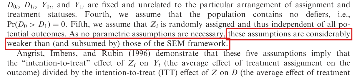
(S3) The five IV assumptions. p. 495 (PDF p. 4): “Using an IV estimator, we may estimate the LATE using five assumptions, as explicated by Angrist, Imbens, and Rubin (1996). First, we assume that the exclusion restriction is valid, or that $Z_i$ only affects $Y_i$ through $D_i$. Second, we assume that $Z_i$ to some degree predicts $D_i$. Third, we invoke the stable unit treatment value assumption, which states that the potential outcomes $D_{0i}$, $D_{1i}$, $Y_{0i}$, and $Y_{1i}$ are fixed and unrelated to the particular arrangement of assignment and treatment statuses. Fourth, we assume that the population contains no defiers, i.e., $\Pr(D_0 > D_1) = 0$. Fifth, we assume that $Z_i$ is randomly assigned and thus independent of all potential outcomes.”
(S4) Rendering of (S1)–(S3) used in every target (the article prints no display for it; all validators use it). The observed variables are $D = D_0 + Z(D_1 - D_0)$ and $Y = Y_0 + D(Y_1 - Y_0)$ (exclusion and SUTVA); relevance is $\mathrm{E}(D|Z=1) - \mathrm{E}(D|Z=0) \neq 0$; no defiers is $\Pr(D_0 > D_1) = 0$; random assignment is: $Z$ is independent of $(D_0, D_1, Y_0, Y_1)$, and of $(\mathbf{X}, D_0, D_1, Y_0, Y_1)$ where covariates appear (p. 496: “so that $\mathbf{X} \perp\!\!\!\perp Z$”), with $0 < \Pr(Z = 1) < 1$. Abbreviations used in the targets and not in the article: $\tau = Y_1 - Y_0$ and $C = \mathbf{1}\{D_1 > D_0\}$.
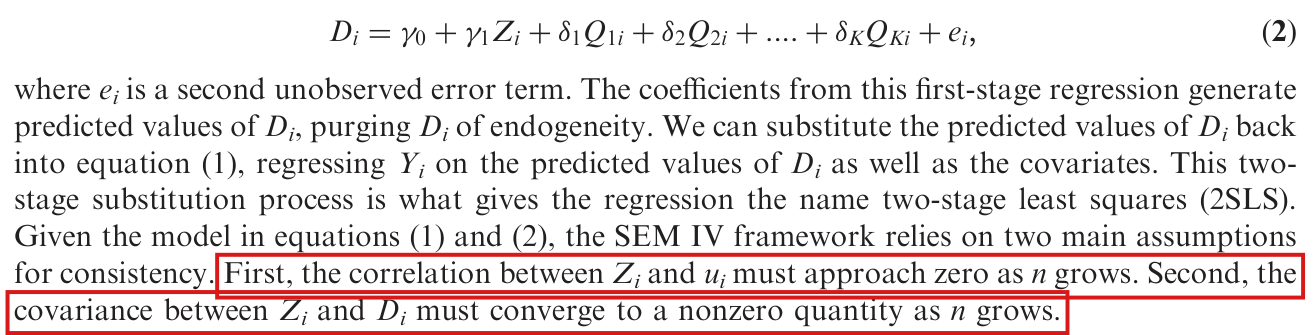
(S5) SEM framework. p. 493 (PDF p. 2), Section 2.1: “The SEM interpretation of IV estimation posits a linear, additive relationship between an outcome variable ($Y_i$), an endogenous treatment variable ($D_i$), covariates ($Q_{1i}, Q_{2i}....Q_{Ki}$), and an unobserved error term ($u_i$) for each unit $i$, such that $$Y_i = \beta_0 + \beta_1 D_i + \lambda_1 Q_{1i} + \lambda_2 Q_{2i} + .... + \lambda_K Q_{Ki} + u_i. \qquad (1)$$” p. 494 (PDF p. 3): “The first equation, or the “first stage,” is a regression of the endogenous variable on the instrument and covariates: $$D_i = \gamma_0 + \gamma_1 Z_i + \delta_1 Q_{1i} + \delta_2 Q_{2i} + .... + \delta_K Q_{Ki} + e_i, \qquad (2)$$ where $e_i$ is a second unobserved error term. [...] Given the model in equations (1) and (2), the SEM IV framework relies on two main assumptions for consistency. First, the correlation between $Z_i$ and $u_i$ must approach zero as $n$ grows. Second, the covariance between $Z_i$ and $D_i$ must converge to a nonzero quantity as $n$ grows. Note, however, that whereas the endogenous variable and covariates in equation (1) are indexed by the subscript $i$, their coefficients (the βs and λs) are not. In other words, the SEM framework assumes constant treatment effects, so that the effect of the treatment is identical for each unit $i$.”
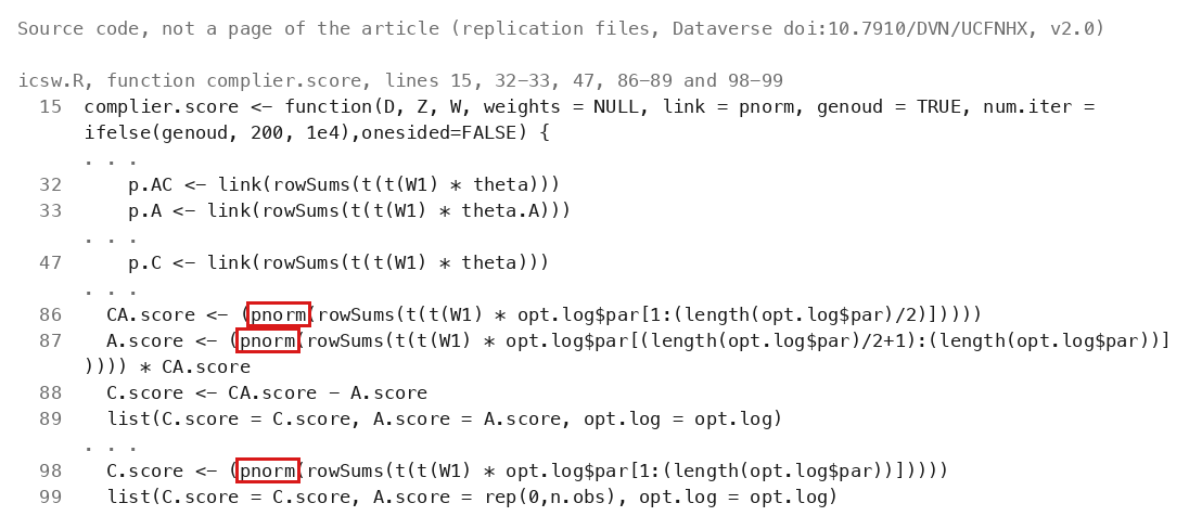
(S6) Compliance score and nested model. p. 496 (PDF p. 5), Section 3.1: “The compliance score is a latent pretreatment covariate that represents the probability of being a complier, conditional on a unit’s pretreatment covariate profile $\mathbf{X}$ (so that $\mathbf{X} \perp\!\!\!\perp Z$). The compliance score for unit $i$, $P_{Ci} = \Pr(D_1 > D_0|\mathbf{X} = \mathbf{x}_i)$, where $\mathbf{x}_i$ is the covariate vector for unit $i$.” Equations (5) and (6), p. 496: $$P_{A,C,i} = \Pr(D_1 > D_0 \cup D_0 = 1|\mathbf{X} = \mathbf{x}_i) = F(\theta_{\mathbf{A,C}}\mathbf{x_i}), \qquad (5)$$ “where $P_{A,C,i}$ is the conditional probability that unit $i$ is either a complier or an always-taker, $\theta_{\mathbf{A,C}}$ is a vector of coefficients to be estimated, and $F(\cdot)$ is the cumulative distribution function (CDF) for an arbitrary distribution. For the purposes of this article, we use a probit model, so $F(\cdot) = \Phi(\cdot)$, where $\Phi$ is the Normal CDF. Second, we similarly specify $$P_{A|A,C,i} = \Pr(D_0 = 1|D_1 > D_0 \cup D_0 = 1, \mathbf{X} = \mathbf{x}_i) = F(\theta_{\mathbf{A|A,C}}\mathbf{x_i}), \qquad (6)$$ where $P_{A|A,C,i}$ is the conditional probability that unit $i$ is an always-taker conditional on it being either an always-taker or a complier, and $\theta_{\mathbf{A|A,C}}$ are coefficients to be estimated.” Equation (7), p. 497 (PDF p. 6): “[...] our third assumption: $D_i$ is Bernoulli distributed. Then the likelihood for any unit $i$, $$L(P_{A|A,C,i}, P_{A,C,i}|D, Z) = (P_{A,C,i}(1 - P_{A|A,C,i})Z_i + P_{A,C,i}P_{A|A,C,i})^{D_i}(1 - P_{A,C,i}(1 - P_{A|A,C,i})Z_i - P_{A,C,i}P_{A|A,C,i})^{1-D_i}. \qquad (7)$$ Combining equations (5), (6), and (7), $L(\theta_{\mathbf{A,C}}, \theta_{\mathbf{A|A,C}}|D, Z) = \Pi_{i=1}^{n}((F(\theta_{\mathbf{A,C}}\mathbf{x_i})(1 - F(\theta_{\mathbf{A|A,C}}\mathbf{x_i}))Z_i + F(\theta_{\mathbf{A,C}}\mathbf{x_i})F(\theta_{\mathbf{A|A,C}}\mathbf{x_i}))^{D_i}(1 - F(\theta_{\mathbf{A,C}}\mathbf{x_i})(1 - F(\theta_{\mathbf{A|A,C}}\mathbf{x_i}))Z_i - F(\theta_{\mathbf{A,C}}\mathbf{x_i})F(\theta_{\mathbf{A|A,C}}\mathbf{x_i}))^{1-D_i})$. Thus the ML estimate of $\{\theta_{\mathbf{A,C}}, \theta_{\mathbf{A|A,C}}\}$, $$\{\hat\theta_{\mathbf{A,C}}, \hat\theta_{\mathbf{A|A,C}}\} = \underset{\theta_{\mathbf{A,C}},\theta_{\mathbf{A|A,C}}}{\mathrm{argmax}}\left[L(\theta_{\mathbf{A,C}}, \theta_{\mathbf{A|A,C}}|D, Z)\right].$$ After estimating $\theta_{\mathbf{A,C}}$ and $\theta_{\mathbf{A|A,C}}$, we may estimate the compliance score for unit $i$, $$\hat{P}_{Ci} = \widehat{\Pr}(D_1 > D_0|\mathbf{X} = \mathbf{x}_i) = F(\hat\theta_{\mathbf{A,C}}\mathbf{x_i})(1 - F(\hat\theta_{\mathbf{A|A,C}}\mathbf{x_i})).$$” (On the page this display is followed by a superscript 3, which is the marker of footnote 3 and not an exponent.) The displays between (6) and (7) that carry the misprints of finding P029-E009 are transcribed in P029-T18.
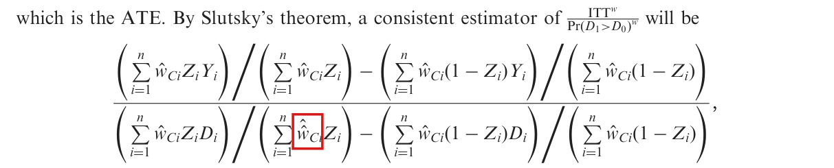
(S7) ICSW estimator. p. 498 (PDF p. 7), Section 3.3: “In the bivariate case (when there are no covariates), the estimator is simple. Define $\hat{w}_{Ci} = 1/\hat{P}_{Ci}$. The ICSW estimator $\hat\tau_{\mathrm{ATE}} =$ $$\frac{(\sum_{i=1}^{n}\hat{w}_{Ci}Z_iY_i)/(\sum_{i=1}^{n}\hat{w}_{Ci}Z_i) - (\sum_{i=1}^{n}\hat{w}_{Ci}(1 - Z_i)Y_i)/(\sum_{i=1}^{n}\hat{w}_{Ci}(1 - Z_i))}{(\sum_{i=1}^{n}\hat{w}_{Ci}Z_iD_i)/(\sum_{i=1}^{n}\hat{w}_{Ci}Z_i) - (\sum_{i=1}^{n}\hat{w}_{Ci}(1 - Z_i)D_i)/(\sum_{i=1}^{n}\hat{w}_{Ci}(1 - Z_i))}.$$ An equivalent estimator may be derived using weighted 2SLS (with weights $\hat{w}_{Ci}$). As with the simple 2SLS case, covariates may also be included to reduce sampling variability without any consequence for the asymptotic bias of the estimator.”
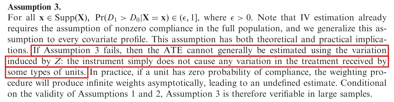
(S8) Assumptions 1–3. p. 498 (PDF p. 7), Section 3.4: “In order to consistently estimate the ATE using ICSW, three additional assumptions are required. In the appendix, we demonstrate that ICSW is consistent under Assumptions 1–3, along with the IV assumptions and suitable regularity conditions.” p. 499 (PDF p. 8): “Assumption 1. Latent ignorability of compliance with respect to treatment effect heterogeneity (Frangakis and Rubin 1999; Esterling, Neblo, and Lazer 2011) holds. Assumption 1 entails that, for all $\mathbf{x} \in \mathrm{Supp}(\mathbf{X})$, $\mathrm{E}(Y_1 - Y_0|\mathbf{X} = \mathbf{x}) = \mathrm{E}(Y_1 - Y_0|D_1 > D_0, \mathbf{X} = \mathbf{x})$: the expected value of the treatment effect conditional on a covariate profile is equal to the expected value of the treatment effect conditional on a covariate profile and compliance. Put simply, the ATE for all units with a covariate profile $\mathbf{x}$ is equal to the ATE for compliers with a covariate profile $\mathbf{x}$.” p. 500 (PDF p. 9): “Assumption 2. Consistency of $\hat{P}_{Ci}$ for $P_{Ci}$. Assumption 2 amounts to requiring proper specification of the ML estimator. Application of a flexible parametrization of the covariates in $\mathbf{X}$, as is possible with large samples, will necessarily yield consistency, so long as the rate of growth in the number of estimated parameters is sufficiently slow in $n$. In the case of a saturated model and $F(.)$ as the normal CDF, $\hat{P}_{Ci}$ will be unbiased for the conditional probability of compliance.” p. 500: “Assumption 3. For all $\mathbf{x} \in \mathrm{Supp}(\mathbf{X})$, $\Pr(D_1 > D_0|\mathbf{X} = \mathbf{x}) \in (\epsilon, 1]$, where $\epsilon > 0$. Note that IV estimation already requires the assumption of nonzero compliance in the full population, and we generalize this assumption to every covariate profile.”
(S9) Appendix notation. p. 504 (PDF p. 13): “For clarity, we remove $i$ subscripts to denote all units subject to any conditional probabilities articulated.” p. 499 (PDF p. 8): “where $f(.)$ is the population pdf of $\mathbf{X}$, $g(.)$ is the subpopulation pdf of $\mathbf{X}$ among compliers, and $\Omega = \mathrm{Supp}(\mathbf{X})$.” The article writes integrals against the density $f$; the validators’ witnesses use covariates with finitely many values, for which $f(\mathbf{x}) = \Pr(\mathbf{X} = \mathbf{x})$ and the integrals are sums.
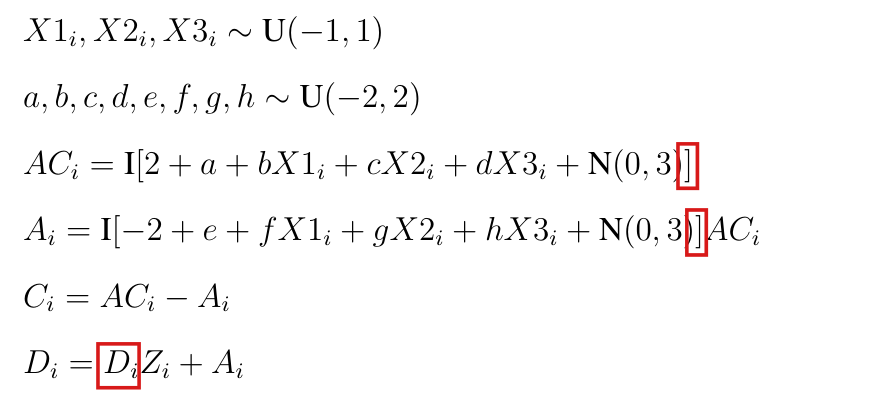
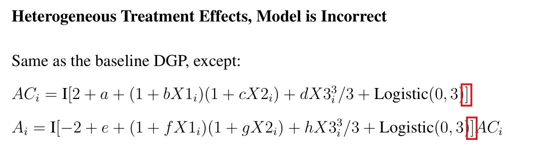
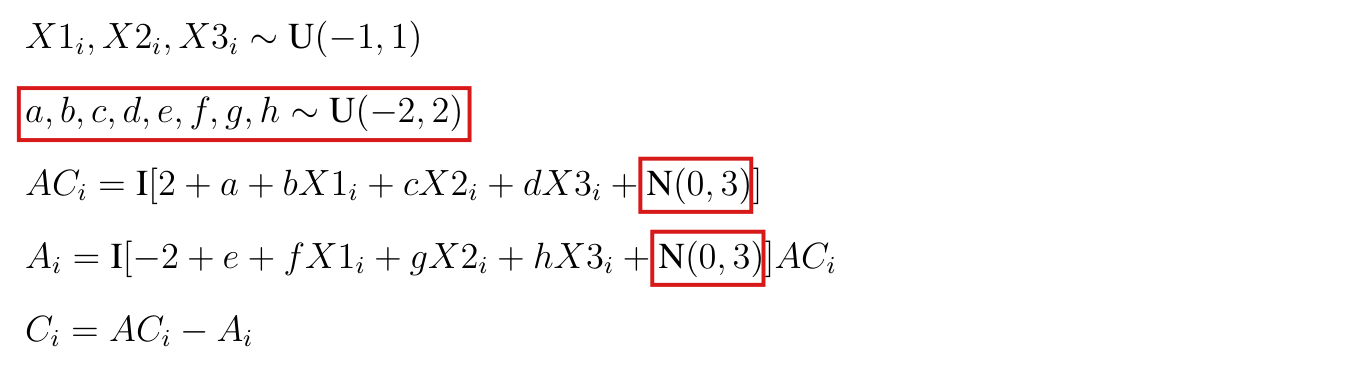
(S10) Simulation designs (supplement). Supplement p. A1, ‘Baseline Data Generating Process’ (as printed; the misprints are the subject of P029-T19): $X1_i, X2_i, X3_i \sim \mathrm{U}(-1, 1)$; $a, b, c, d, e, f, g, h \sim \mathrm{U}(-2, 2)$; $AC_i = \mathbf{I}[2 + a + bX1_i + cX2_i + dX3_i + \mathrm{N}(0, 3)]$; $A_i = \mathbf{I}[-2 + e + fX1_i + gX2_i + hX3_i + \mathrm{N}(0, 3)]AC_i$; $C_i = AC_i - A_i$; $D_i = D_iZ_i + A_i$; $Y_{0i} = 5AC_i + \mathrm{N}(0, 1)$; $\tau_i = 5 \times (1 + X1_i + X2_i + X3_i)$; $Y_i = Y_{0i} + \tau_iD_i$. “We observe and use $X1_i, X2_i, X3_i$ both as covariates in 2SLS, and for the compliance score model.” Supplement p. A2, under the heading ‘Heterogeneous Treatment Effects, Conditioning on Random Noise’: “Same as baseline, except: $X1'_i, X2'_i, X3'_i \sim U(-1, 1)$ are the observed covariates, which are entirely independent from $X1_i, X2_i, X3_i$.” Under the heading ‘Homogeneous Treatment Effects, Conditioning on Random Noise’: “Same as the previous DGP, except: $\tau_i = 5, \forall i$.”
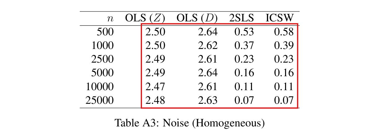
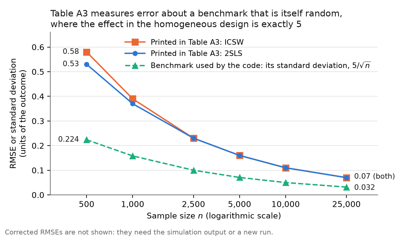
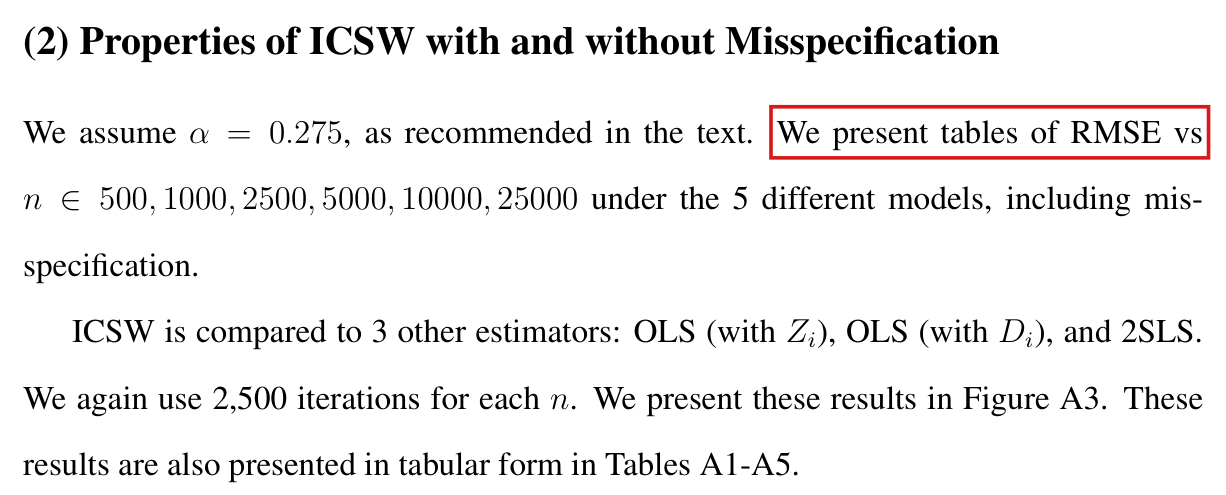
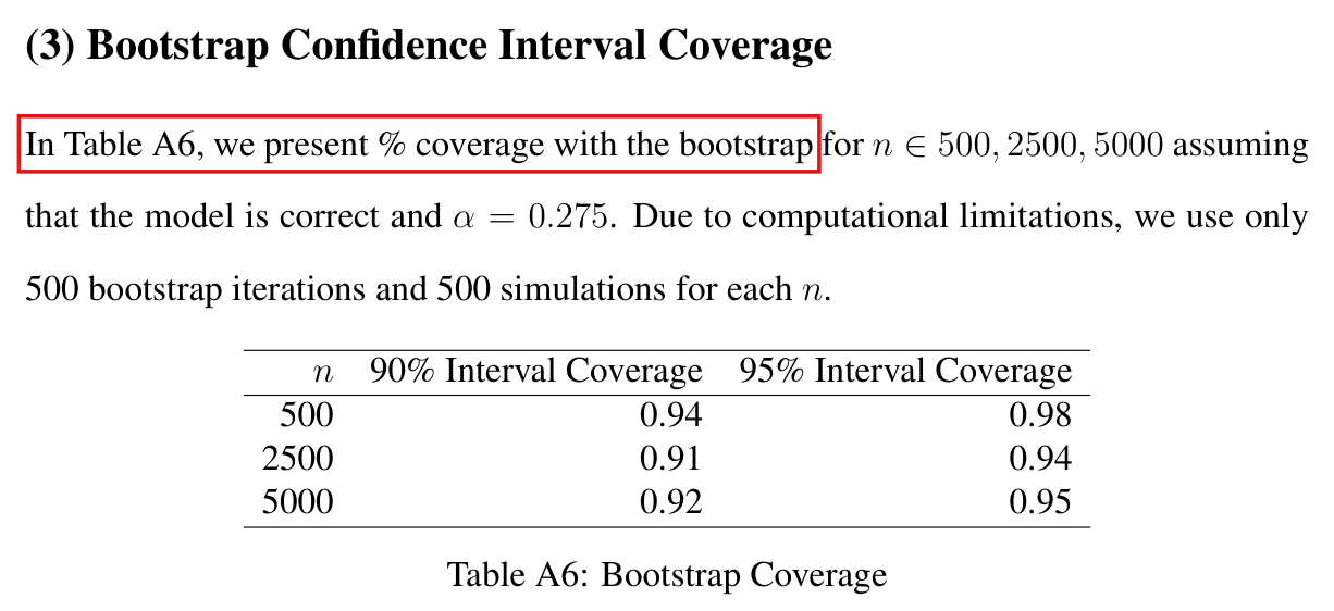
Effective claim (source TeX): [Printed statements] Supplement p. A2, under the heading ‘Homogeneous Treatment Effects, Conditioning on Random Noise’: “Same as the previous DGP, except: $\tau_i = 5, \forall i$.” (the previous design is quoted in (S10)). Supplement p. A5: “We assume $\alpha = 0.275$, as recommended in the text. We present tables of RMSE vs $n \in 500, 1000, 2500, 5000, 10000, 25000$ under the 5 different models, including misspecification. ICSW is compared to 3 other estimators: OLS (with $Z_i$), OLS (with $D_i$), and 2SLS. We again use 2,500 iterations for each $n$. We present these results in Figure A3. These results are also presented in tabular form in Tables A1-A5.” “Table A3: Noise (Homogeneous)”, p. A7, columns $n$; OLS ($Z$); OLS ($D$); 2SLS; ICSW: $500$: $2.50$, $2.64$, $0.53$, $0.58$; $1000$: $2.50$, $2.62$, $0.37$, $0.39$; $2500$: $2.49$, $2.61$, $0.23$, $0.23$; $5000$: $2.49$, $2.64$, $0.16$, $0.16$; $10000$: $2.47$, $2.61$, $0.11$, $0.11$; $25000$: $2.48$, $2.63$, $0.07$, $0.07$.
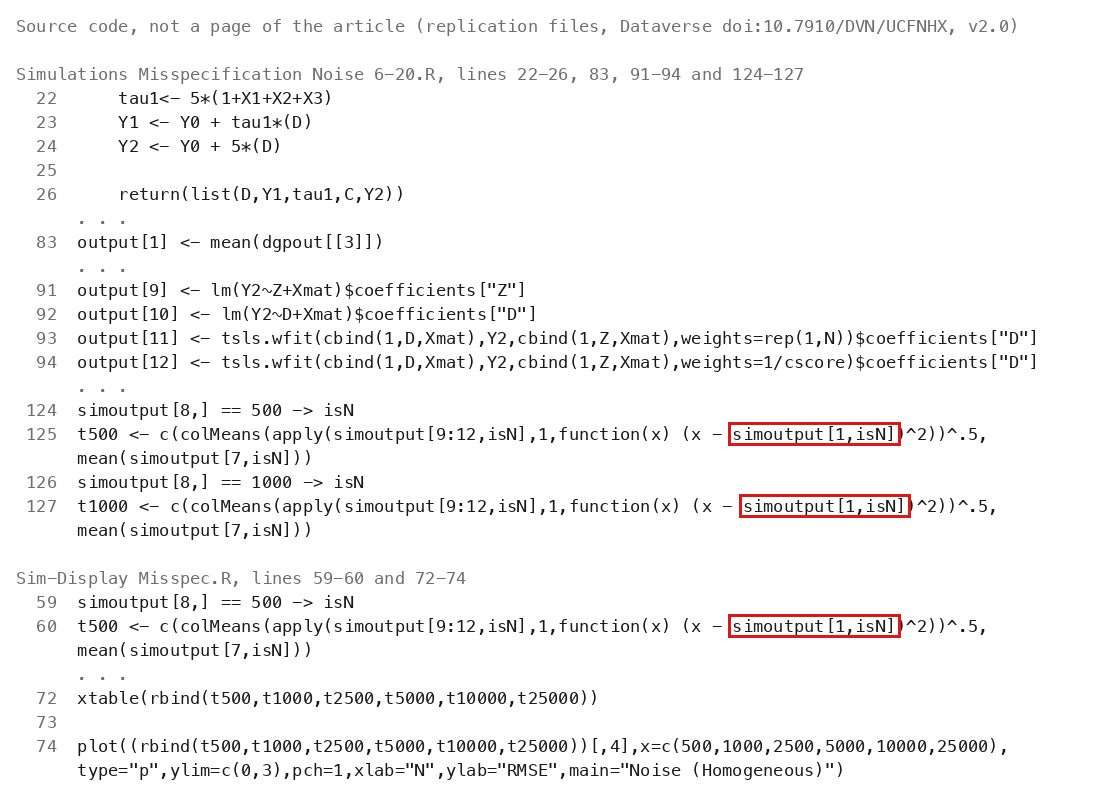
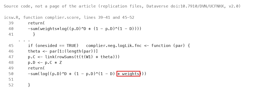
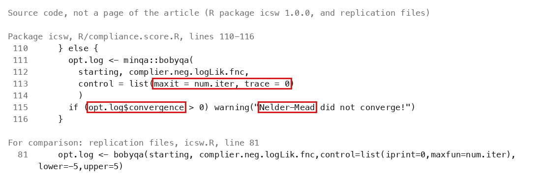
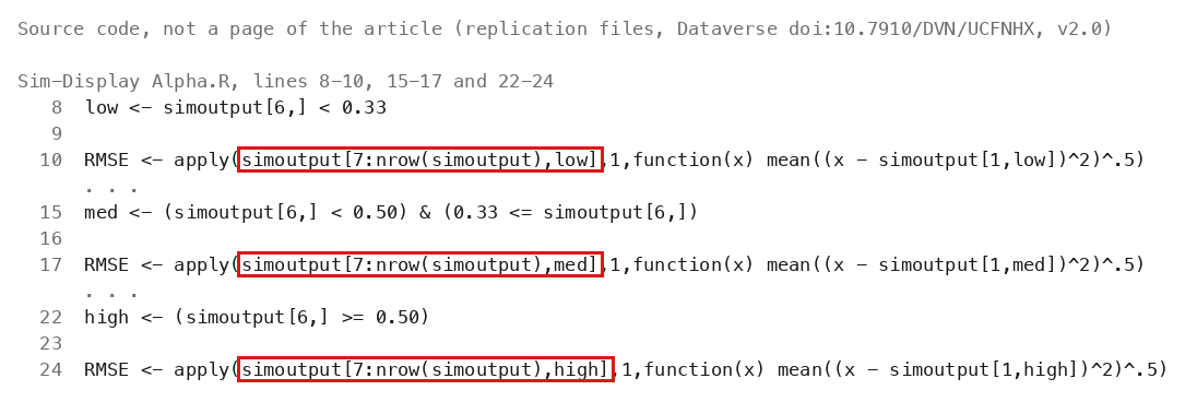
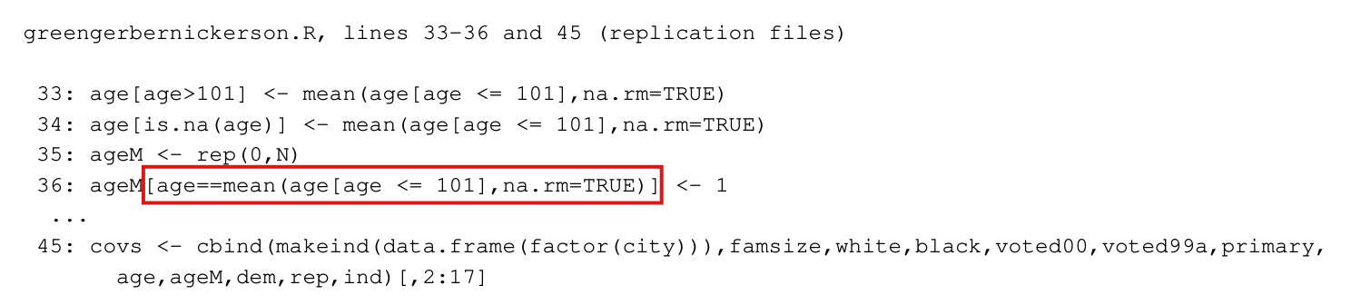
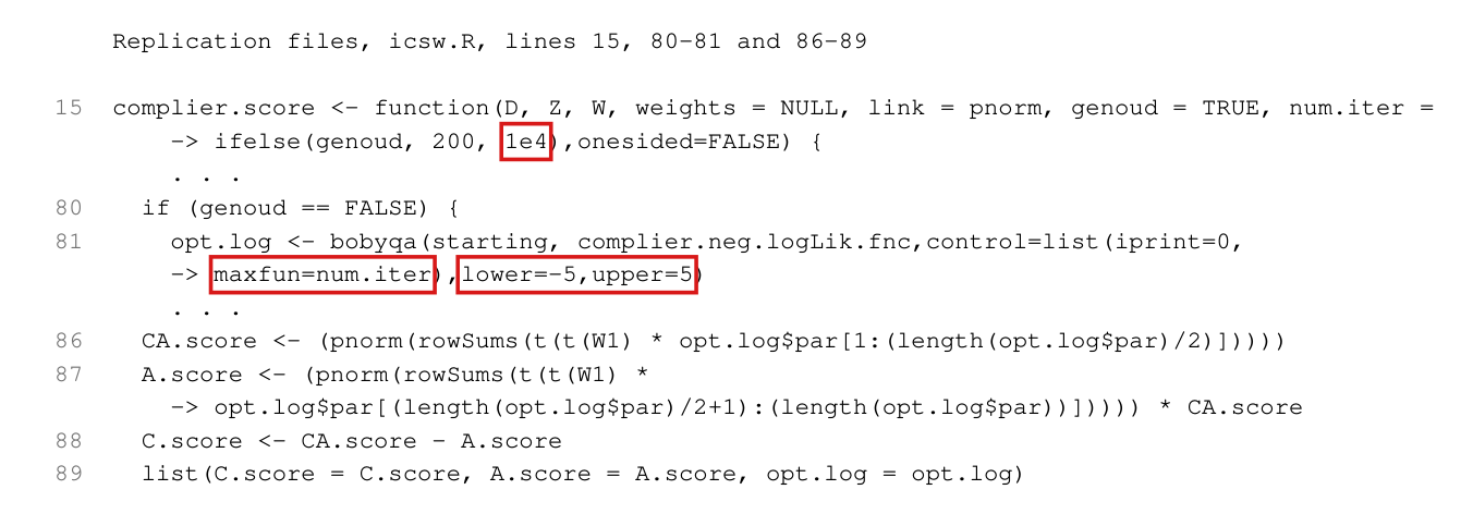
[The computation behind the table (deposited code, transcribed from the staged file; the R operator \$ is written with a backslash)] In the data-generating function: `tau1<- 5*(1+X1+X2+X3)`; `Y1 <- Y0 + tau1*(D)`; `Y2 <- Y0 + 5*(D)`; `return(list(D,Y1,tau1,C,Y2))`. In the iteration: `Y2 <- dgpout[[5]]`; `output[1] <- mean(dgpout[[3]])`; `output[11] <- tsls.wfit(cbind(1,D,Xmat),Y2,cbind(1,Z,Xmat),weights=rep(1,N))\$coefficients["D"]`; `output[12] <- tsls.wfit(cbind(1,D,Xmat),Y2,cbind(1,Z,Xmat),weights=1/cscore)\$coefficients["D"]`. In both reporting scripts, for each $n$: `t500 <- c(colMeans(apply(simoutput[9:12,isN],1,function(x) (x - simoutput[1,isN])^2))^.5,mean(simoutput[7,isN]))`.
[Reading in real arithmetic] For estimator $j$ (rows 9–12, all fitted to the homogeneous outcome $Y2$) and the $R$ replicates with a given $n$, the code returns $\sqrt{R^{-1}\sum_{r=1}^{R}(t_{jr} - B_r)^2}$, where $t_{jr}$ is the estimate in replicate $r$ and $B_r = \frac{1}{n}\sum_{i=1}^{n}5(1 + X1_i + X2_i + X3_i)$ is that replicate's sample mean of the heterogeneous effects of the companion design. In the homogeneous design every unit's effect is $5$, so the quantity the table is presented as is $\sqrt{R^{-1}\sum_{r=1}^{R}(t_{jr} - 5)^2}$.
[Counterexample: the two scoring rules differ, in either direction, on admissible inputs] $n = 500$; $a = b = c = d = e = f = g = h = 0$; for every unit the latent covariates are $(X1_i, X2_i, X3_i) = (1/5, 0, 0)$ and the three normal draws entering $AC_i$, $A_i$ and $Y_{0i}$ are $\varepsilon^{AC}_i = \varepsilon^{A}_i = 0$ and $\varepsilon^{Y}_i$ as specified below. The units come in 50 identical blocks of ten: the observed noise covariates $(W1, W2, W3)$ run through the five profiles $(0,0,0)$, $(1/2,0,0)$, $(0,1/2,0)$, $(0,0,1/2)$, $(-1/2,-1/2,-1/2)$, each profile appearing first with $Z = 0$ and then with $Z = 1$ (so 250 units have $Z = 1$). With the corrected indicator rule of P029-T19: $AC_i = \mathbf{I}[2 > 0] = 1$, $A_i = \mathbf{I}[-2 > 0]\cdot 1 = 0$, $C_i = 1$, $D_i = Z_i$, $Y_{0i} = 5 + \varepsilon^{Y}_i$, $Y2_i = Y_{0i} + 5D_i$, $\mathtt{tau1}_i = 5(1 + 1/5) = 6$, hence $B = 6$. Let $Q$ be the $500 \times 5$ matrix with rows $(1, Z_i, W1_i, W2_i, W3_i)$; here the regressor matrix $(1, D_i, W1_i, W2_i, W3_i)$ equals $Q$.
(a) $Q^{\mathsf T}Q = \begin{pmatrix} 500 & 250 & 0 & 0 & 0 \\ 250 & 250 & 0 & 0 & 0 \\ 0 & 0 & 50 & 25 & 25 \\ 0 & 0 & 25 & 50 & 25 \\ 0 & 0 & 25 & 25 & 50 \end{pmatrix}$, with determinant $62500^2 = 3906250000 \neq 0$; so the unweighted 2SLS coefficient vector (regressors $Q$, instruments $Q$) is $(Q^{\mathsf T}Q)^{-1}Q^{\mathsf T}Y2$.
(b) [‘Perfect’ input] $\varepsilon^{Y}_i = 0$ for all $i$: $Y2_i = 5 + 5Z_i$, $Q^{\mathsf T}Y2 = (3750, 2500, 0, 0, 0)^{\mathsf T}$, the 2SLS coefficient vector is $(5, 5, 0, 0, 0)^{\mathsf T}$ and the estimate of the effect is $t = 5$. The coded squared error is $(t - B)^2 = 1$; the squared error about the true effect is $(t - 5)^2 = 0$.
(c) [‘Opposite’ input] $\varepsilon^{Y}_i = Z_i$: $Y2_i = 5 + 6Z_i$, $Q^{\mathsf T}Y2 = (4000, 2750, 0, 0, 0)^{\mathsf T}$, the coefficient vector is $(5, 6, 0, 0, 0)^{\mathsf T}$ and $t = 6$. Every unit's effect is still $5$. The coded squared error is $(t - B)^2 = 0$; the squared error about the true effect is $(t - 5)^2 = 1$.
(d) For any positive weights the weighted 2SLS coefficient vector with regressors and instruments both equal to $Q$ and outcome $Qb$ is $b$; so in (b) the ICSW fit (row 12) also returns $5$ whatever positive scores are estimated.
: T5Statement
Theorem: SAP.P029a.T5
Statement hash: d1278a217536e79e5c9da7c3856565655bfd9a551426c2d4b5a9a9c59be4c527
Statement definition: SAP.P029a.T5Statement
Certificate. 20261104T173414Z
Declaration review: faithful; 2026-11-04T18:06:58Z; binding v2
Evidence scope: Certification checks formal proof objects. Statement fidelity is a model judgment. Author review is separate.
Proof dependencies: Independently extracted
Manifest annotation reconciliation: Effective use follows the source-bound dependency observation; original annotations are retained in the crosswalk.
AronowAudit.P029.normal_equation_exact_recovery: observed used
AronowAudit.P029.rmse_design_gram: observed used
Source and evidence metadata · sap-2026-11-08-assured-release