LLM-generated corrections to the published research of P. M. Aronow

Journal article P030

Corrections to: A General Method for Detecting Interference Between Units in Randomized Experiments

P. M. Aronow (2012). A General Method for Detecting Interference Between Units in Randomized Experiments. Sociological Methods and Research 41(1):3–16.

DOI
10.1177/0049124112437535
Audited edition
Sociological Methods and Research, 2012, 41(1):3–16; 14 pages in the audited file
SHA-256 of the audited file
c7126d7c6415ac441f23e5137d158ae54286e73928f217ee9e5a2d1a0e4136fd
Permanent address
https://pmaronow.github.io/llm-audit/works/P030/

Summary

The article proposes a test for interference between units in a randomized experiment: the treatment of a fixed subset of units is held at its realized value, the other units are re-randomized, and a statistic is compared with its distribution over these re-randomizations. In a voter-turnout mailing experiment the article reports rejection of the hypothesis of no interference (p<0.001p<0.001). 11 entries are classified as errors (2 Moderate, 9 Minor, none Major or Critical), and 2 are clarity notes. The most consequential is P030-E001: the two-tailed rule printed after Equation (2) can reject more often than its nominal level.

What was and was not checked

I examined all 14 pages of the article. It has no appendix, and I had no supplement. The list below states what I examined and what held up. These checks do not establish that the rest of the article is correct.

  • The method. The three expectations of the number of proximal treated units on p. 5 hold: E(Pi)=KiM/NE(P_i)=K_iM/N, E(Pi∣Zi=1)=Ki(M−1)/(N−1)E(P_i\mid Z_i=1)=K_i(M-1)/(N-1) and E(Pi∣Zi=0)=KiM/(N−1)E(P_i\mid Z_i=0)=K_iM/(N-1). Under the hypothesis of no interference, the outcomes of the fixed units are the same for every assignment in Ω′\Omega', and the conditional randomization argument on p. 6 follows. The one-tailed pp value of Equation (2) is valid when the assignments in Ω′\Omega' are equally likely and each is counted. This condition holds under complete randomization when the fixed subset is a uniform sample of fixed size from the control units, which is the design of the simulations and the choice that the article recommends. The rule of thumb in Equation (3) selects half of the control units, up to integer rounding, as stated. The definition of the Spearman statistic in words on p. 8 is correct, and the displayed formula is the subject of P030-E004.
  • The worked example. I recomputed the outcomes, the distances and the six rows of Table 1 exactly; the correlations and pp value agree to the printed rounding (ρ=−0.949\rho=-0.949, p=0.333p=0.333).
  • The simulations. The decay functions plotted in the left panels of Figure 2 agree with the printed formulas. A new implementation of the Gaussian design from the text, with fewer replications than the article reports, gave a two-tailed rejection rate of 0.8330.833 at α=0.05\alpha=0.05 with N=400N=400 (the article reports 83%). It also matched the Gaussian and inverse-square panels of Figure 2 at the sample sizes tried, within Monte Carlo uncertainty and the precision of reading the figure. The linear panel did not match (P030-N006). My larger-sample inverse-square simulations also did not establish the reported rejection rate above 95% near N=5,000N=5{,}000 (P030-N005).
  • The application. The description of the experiment of Gerber, Green and Larimer (2008) and of its four mailings agrees with the public replication files of that study, and the difference in means of 8.1 percentage points matches their counts. In Figure 3, the dashed line appears near the reported ρ=0.0061\rho=0.0061, well to the left of the visible histogram, which is consistent with the reported p<0.001p<0.001. The binned figure does not establish the exact tail count.
  • The references. Every work cited in the text appears in the reference list, and every listed work is cited.

The following were not checked, or could not be.

  • I had no code for the article’s simulations or for its reanalysis of the turnout experiment. The simulations were compared only with new implementations written from the text, on a smaller scale than the 10,000 simulations of 5,000 randomizations each that the article reports. The Kolmogorov–Smirnov pp value of 0.6610.661 cannot be checked without the original draws.
  • The household locations used in the application are not part of the public release of the turnout experiment. For this reason ρ=0.0061\rho=0.0061, the summaries of DnearestD_{\mathit{nearest}} and the reference distribution in Figure 3 were not recomputed, and the scheme used for the 1,000 conditional randomizations was not examined.
  • I did not read the works that the article cites. The quotations and the results attributed to them were not checked. These include the indirect effect of about 0.5 percentage points and the finding of McConnell et al. (2010), on which the article rests its statement that the bias from interference is likely negligible in such experiments.

Headline claims and related corrections

  1. Holding the treatment of a chosen fixed subset at its realized value and re-randomizing the remaining units gives a conditional randomization test, with a statistic of the analyst's choice, whose pp value is the exact significance level for the null of no interference; the procedure is 'an exact, distribution-free test'.

    Abstract; introduction (printed p. 5); Method (printed pp. 6–7): H0′′H_{0''}, Equation (1), Equation (2) and the two-tailed rule after it; Table 1; Figure 3

    See P030-E001, P030-E002, P030-N002.

  2. Because the fixed units' own treatment is held constant, any dependence of their outcomes on the assignment of the other units can only be interference, so rejection is sufficient for detecting interference and is not confounded with direct effects.

    Introduction (printed pp. 5–6); Method (printed p. 6): H0′′H_{0''} and the sentence 'Because Zfixed=Zfixed′Z_{\mathit{fixed}}=Z'_{\mathit{fixed}} ... H0′′H_{0''} must be rejected'

    See P030-N001.

  3. Relating outcomes to proximity to treated units naively does not follow from the randomization: expected exposure depends on the number of neighbours and on own treatment, and under the null the statistic is not centred at zero (all six ρ0\rho_0 values negative in the example; null centre about 0.014 in the application). Conditional randomization accounts for these design-induced relationships.

    The three exposure expectations on printed p. 5; Table 1; Figure 3

    See P030-E004, P030-N003.

  4. Simulations show the method behaves as intended: without interference the pp values are approximately uniform (Kolmogorov–Smirnov p=0.661p=0.661); with interference under a Gaussian distance decay and N=400N=400 the two-tailed test at α=0.05\alpha=0.05 rejects in 83% of simulations; detection rises with NN under all three decay forms and appears to converge to 100%.

    Abstract; Simulation Studies (printed pp. 10-12); Figure 1; Figure 2

    See P030-E001, P030-E006, P030-E007, P030-E010, P030-N005, P030-N006.

  5. Applied to the Gerber, Green and Larimer (2008) mailing experiment with the civic duty, Hawthorne and self arms as the fixed subset, the test detects interference from the neighbors treatment: observed ρ=0.0061\rho=0.0061 lies far to the left of a null distribution centred near 0.014 (1,000 conditional randomizations), p<0.001p<0.001. The same analysis reports a direct effect of about 8.1 percentage points.

    Abstract; Application (printed pp. 12–14); Figure 3; the reported NN, NfixedN_{\mathit{fixed}}, NcontrolN_{\mathit{control}}, NtreatmentN_{\mathit{treatment}}; the difference-in-means estimate

    See P030-E008, P030-E009.

  6. The method can be applied after an experiment with a suitably chosen fixed subset; for a binary treatment a random subset of units from one condition is recommended, with NfixedN_{\mathit{fixed}} chosen to maximize NfixedNZ=0,variantNZ=1,variantN_{\mathit{fixed}}N_{Z=0,\mathit{variant}}N_{Z=1,\mathit{variant}}, which for a random sample of controls means fixing half of the control units.

    Method and Practical Considerations (printed pp. 6-9); Equation (3); conclusion (printed p. 15)

  7. Although interference is detected, the resulting bias in mailing-and-turnout experiments is likely negligible, because the indirect effects found elsewhere are small (about 0.5 percentage points for the neighbors treatment) or absent.

    Application (printed p. 14); Conclusion (printed p. 15); Aronow (2011) working paper; McConnell et al. (2010)

  8. An ex post interference diagnostic can inform future experimental design and help assess whether standard treatment-effect analyses are vulnerable to interference.

    Conclusion (printed p. 15); Application (printed pp. 14-15); Equations (1)-(2); Figure 3

    See P030-E001.

Corrections

Moderate (2)

A real substantive error with limited reach.

The two-tailed rule printed after Equation (2) can reject with probability greater than α\alpha under the null hypothesis when the reference distribution is discrete; the upper side of the rule must use the inclusive upper-tail probability Pr⁡(t0≥t)\Pr(t_0\ge t).

The two-tailed rule after Equation (2), p. 7 (PDF p. 5)

See also under Formal statements (Lean): P030-T1, P030-T2, P030-T3, P030-T4

As printed
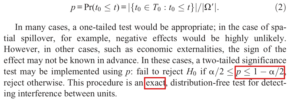
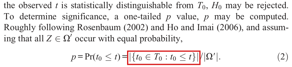
p=Pr⁡(t0≤t)=∣{t0∈T0:t0≤t}∣/∣Ω′∣.(2)p=\Pr(t_0\le t)=|\{t_0\in T_0:t_0\le t\}|/|\Omega'|. \qquad (2)

… In these cases, a two-tailed significance test may be implemented using pp: fail to reject H0H_0 if α/2≤p≤1−α/2\alpha/2\le\colorbox{#ffe58a}{$p\le 1-\alpha/2$}, reject otherwise. This procedure is an exact, distribution-free test for detecting interference between units.

The problem

The rule uses only the lower-tail probability p=Pr⁡(t0≤t)p=\Pr(t_0\le t) of Equation (2), which includes the observed value. On the lower side the rule rejects when p<α/2p<\alpha/2, and under H0H_0 this event has probability at most α/2\alpha/2. On the upper side it rejects when p>1−α/2p>1-\alpha/2, that is, when Pr⁡(t0>t)<α/2\Pr(t_0>t)<\alpha/2. This is a condition on the strict upper tail, which leaves out the probability that the reference distribution gives to the observed value. When the reference distribution is discrete, this probability can be large. In particular, the largest value of the statistic has p=1p=1 and is always rejected, however probable it is. The rule can then reject with probability greater than α\alpha when there is no interference, and the statement that the two-tailed procedure is exact does not hold. Excluding ties does not remove the problem. With nn equally likely distinct values, the rule rejects with probability (2⌈nα/2⌉−1)/n(2\lceil n\alpha/2\rceil-1)/n, which is 1/61/6 for n=6n=6 and α=0.05\alpha=0.05. Not every discrete distribution leads to a rejection probability above the nominal level: for n=5,000n=5{,}000 the same expression equals 249/5000249/5000. The one-tailed pp value of Equation (2) is not affected.

Evidence an exact counterexample

The evidence is three exact counterexamples and a derivation of the corrected rule. All probabilities are exact, and α=1/20\alpha=1/20 throughout.

First, I consider five units on a line at the positions 0,4,8,−1,−20,4,8,-1,-2. The units at 0,4,80,4,8 form the fixed subset; they are never treated, and their outcomes are 0,1,20,1,2 under every assignment. Exactly one of the units at −1-1 and −2-2 is treated, each with probability 1/21/2, and both have outcome 00 under every assignment. No outcome depends on any treatment, so H0H_0 holds. The distances from the fixed units to the treated unit are (1,5,9)(1,5,9) or (2,6,10)(2,6,10), and ρ=1\rho=1 under both assignments. The example therefore satisfies Equation (1) even as it is printed (see P030-E002). Then p=1>39/40p=1>39/40 under both assignments, and the printed rule rejects with probability 1.

Second, I keep the fixed units and place 42 other units at −1,−2,…,−41-1,-2,\ldots,-41 and 99, each with outcome 00 under every assignment. One of them is treated, each with probability 1/421/42. The statistic equals 11 when the treated unit is at a negative position and −1-1 when it is at 99. For ρ=−1\rho=-1 I have p=1/42<1/40p=1/42<1/40, and for ρ=1\rho=1 I have p=1p=1. The printed rule rejects both values, again with probability 1, although the statistic is not constant.

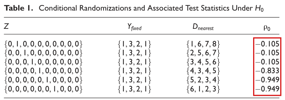
Third, the reference distribution of Table 1 arises without interference when the ten outcomes (1,2,2,2,2,3,2,3,2,1)(1,2,2,2,2,3,2,3,2,1) are the same under every assignment. (The article’s example generates these outcomes with interference; the population used here is a separate one.) The table below lists the six equally likely assignments. The printed rule rejects the three with p=1p=1, which have total probability 1/21/2.

The reference distribution of Table 1 at α=0.05\alpha=0.05, with pL=Pr⁡(t0≤t)p_L=\Pr(t_0\le t) and pU=Pr⁡(t0≥t)p_U=\Pr(t_0\ge t). The printed rule rejects when pL<0.025p_L<0.025 or pL>0.975p_L>0.975; the corrected rule rejects when 2min⁡(pL,pU)≤0.052\min(p_L,p_U)\le 0.05.
Treated unitρ0\rho_0pLp_LpUp_UPrinted ruleCorrected rule
2−0.105-0.105111/21/2rejectdo not reject
3−0.105-0.105111/21/2rejectdo not reject
4−0.105-0.105111/21/2rejectdo not reject
5−0.833-0.8331/21/22/32/3do not rejectdo not reject
6−0.949-0.9491/31/311do not rejectdo not reject
7−0.949-0.9491/31/311do not rejectdo not reject

For the corrected rule, let the reference distribution have the distinct values x1<⋯<xmx_1<\cdots<x_m with probabilities q1,…,qmq_1,\ldots,q_m, and set C0=0C_0=0 and Cj=q1+⋯+qjC_j=q_1+\cdots+q_j. Under H0H_0 the observed statistic tt is a draw from this distribution. If t=xjt=x_j, then pL=Cjp_L=C_j and pU=1−Cj−1p_U=1-C_{j-1}. Fix u∈[0,1]u\in[0,1]. Since the CjC_j increase, the event pL≤up_L\le u consists of the values x1,…,xkx_1,\ldots,x_k, where kk is the largest index with Ck≤uC_k\le u, and its probability is Ck≤uC_k\le u; the event is empty if there is no such index. In the same way, the event pU≤up_U\le u has probability at most uu. Taking u=α/2u=\alpha/2 with 0<α<10<\alpha<1, I obtain

Pr⁡(2min⁡(pL,pU)≤α)≤Pr⁡(pL≤α/2)+Pr⁡(pU≤α/2)≤α.\Pr\bigl(2\min(p_L,p_U)\le\alpha\bigr)\le\Pr(p_L\le\alpha/2)+\Pr(p_U\le\alpha/2)\le\alpha .

In the first inequality, I used the union bound. In the same notation, I have pU=1−pL+Pr⁡(t0=t)p_U=1-p_L+\Pr(t_0=t). The printed rule compares 1−pL1-p_L with α/2\alpha/2 on the upper side, where the corrected rule compares pUp_U.

What survives

The conditional randomization construction and the one-tailed pp value of Equation (2) are valid under the same assumptions, and Table 1 with its p=0.333p=0.333 is unchanged. The application reports a lower-tail p<0.001p<0.001 on p. 13, which the correction does not change; taking that value as given, the corrected two-tailed pp value is below 0.0020.002. The correction needs no new assumption. Its cost is that some two-tailed rejections are withdrawn. With strict endpoints, every rejection by the corrected rule is also a rejection by the printed rule, and in the first example no rejection remains. The article reports two-tailed rejection rates for its simulations (83% on p. 11, and Figure 2). The simulation code is not available, and how these rates change under the corrected rule has not been established.

Corrected

Let pL=Pr⁡(t0≤t)p_L=\Pr(t_0\le t), as in Equation (2), and let pU=Pr⁡(t0≥t)\colorbox{#ffe58a}{$p_U=\Pr(t_0\ge t)$}. Both are computed under the conditional distribution of ZZ on Ω′\Omega', and every assignment is counted, so that tied values of the statistic are retained. In these cases, a two-tailed significance test may be implemented using p2=min⁡{1,2min⁡(pL,pU)}\colorbox{#ffe58a}{$p_2=\min\{1,2\min(p_L,p_U)\}$}: reject H0H_0 if p2≤α\colorbox{#ffe58a}{$p_2\le\alpha$}, fail to reject otherwise. Suppose that the outcomes of the fixed units do not depend on ZvariantZ_{\mathit{variant}}, which is the hypothesis of no interference for these units, and that the probabilities of the assignments in Ω′\Omega' are those of the design. Then this test rejects with conditional probability at most α\alpha, for every finite reference distribution. The procedure is exact in this sense: its level is at most α\alpha in finite samples, and it need not equal α\alpha. The rule that rejects if pL<α/2p_L<\alpha/2 or pU<α/2p_U<\alpha/2 keeps the strict endpoints of the printed rule and has the same property.

The displayed Equation (2), 'p = Pr(t_0 <= t) = |{t_0 in T_0 : t_0 <= t}| / |Omega-prime|', followed by a paragraph of seven lines. A red box marks 'p <= 1 - alpha/2' in the sentence 'fail to reject H_0 if alpha/2 <= p <= 1 - alpha/2, reject otherwise'. A second red box marks the word 'exact' in the sentence 'This procedure is an exact, distribution-free test for detecting interference between units.'
Equation (2) and the paragraph after it, p. 7 (PDF p. 5). The upper condition of the two-tailed rule, p≤1−α/2p\le 1-\alpha/2, and the word “exact” are marked.
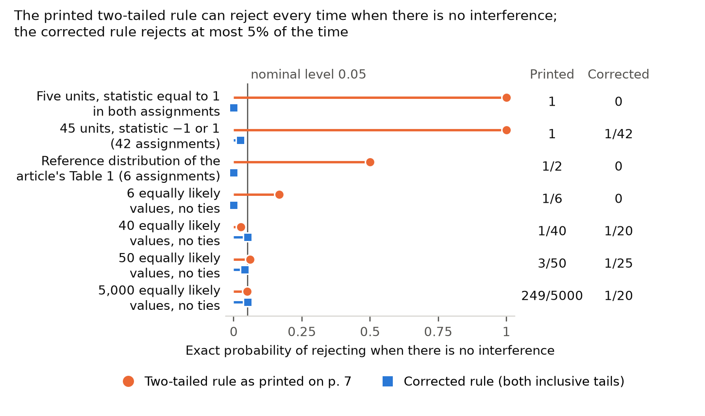
A chart with seven rows and a horizontal axis from 0 to 1 labelled 'Exact probability of rejecting when there is no interference', with a vertical line at the nominal level 0.05. Each row has an orange circle for the two-tailed rule as printed and a blue square for the corrected rule, and the exact values are listed at the right. Five units with the statistic equal to 1 in both assignments: printed 1, corrected 0. Forty-five units with the statistic equal to -1 or 1: printed 1, corrected 1/42. Reference distribution of the article's Table 1: printed 1/2, corrected 0. Six equally likely values with no ties: printed 1/6, corrected 0. Forty values: printed 1/40, corrected 1/20. Fifty values: printed 3/50, corrected 1/25. Five thousand values: printed 249/5000, corrected 1/20.
Exact probability of rejection when there is no interference, at a nominal level of 0.050.05, for the two-tailed rule as printed on p. 7 and for the corrected rule. The first three rows are the three examples above; the last four are reference distributions with nn equally likely distinct values. The printed rule rejects with probability 11, 11, 1/21/2 and 1/61/6 in the first four rows and with probability 3/503/50 for n=50n=50; it is below 0.050.05 for n=40n=40 and n=5,000n=5{,}000. The corrected rule never exceeds 0.050.05.

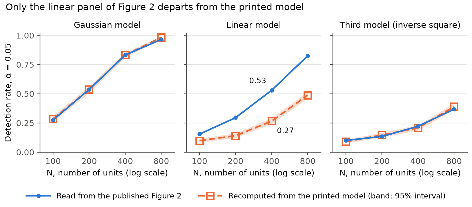
The linear panel of Figure 2 shows higher detection rates than the linear model printed on p. 10 produces: at α=0.05\alpha = 0.05, about 0.53 against 0.27 at N=400N = 400, and 0.83 against 0.49 at N=800N = 800.

Figure 2, linear model panel (middle right), p. 12 (PDF p. 10); the linear model is defined on p. 10 (PDF p. 8)

As printed

Page 10: “The second model is a linear model, for which Θi=∑j((1−δij)Zj[2−dij>0](2−dij))\Theta_i = \sum_j \big( (1 - \delta_{ij}) Z_j [2 - d_{ij} > 0](2 - d_{ij}) \big) and Ψi=∑j((1−δij)[2−dij>0](2−dij))\Psi_i = \sum_j \big( (1 - \delta_{ij}) [2 - d_{ij} > 0](2 - d_{ij}) \big), where [⋅][\cdot] is the Iverson bracket. … In all cases, both Θ\Theta and Ψ\Psi are mean-normalized to one.”

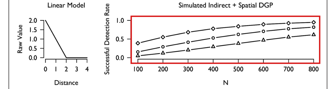
Page 12, Figure 2, linear model panel. The markers have no numerical labels; the values are my readings of the plotted markers, to within 0.01 for circles. At α=0.05\alpha = 0.05 the plotted detection rate is about 0.15 at N=100N = 100, 0.30 at N=200N = 200, 0.53 at N=400N = 400 and 0.83 at N=800N = 800.

The problem

Figure 2 reports, for each of the three models, how often the test detects interference as NN grows. For the linear model the plotted rates lie above the rates that the model produces as it is printed on p. 10: weights 2−dij2 - d_{ij} out to distance 2, the unit’s own term left out, and Θ\Theta and Ψ\Psi each normalized to mean one. At α=0.05\alpha = 0.05 the figure shows about 0.53 at N=400N = 400 and 0.83 at N=800N = 800. For the printed model, I obtain 0.27 and 0.49. At the four checked values of NN, the same recalculation comes within 0.024 of every reading for the Gaussian panel and the panel of the third model. The large gap is specific to the linear panel at those values. Either the plotted linear curves or the printed linear model is not what was simulated, and the paper’s simulation code is not available to say which. A cutoff of 2\sqrt{2} in place of 2 comes closer but overshoots the figure (0.60 at N=400N = 400 and 0.88 at N=800N = 800). It does not identify the simulated model either. Taken from this panel, the power of the test under linear decay is overstated for the model as printed.

Evidence a simulation

A recalculation by simulation of the model as printed. At each of N=100N = 100, 200, 400 and 800, I ran 1,200 independent simulations, each with 5,000 conditional randomizations and the two-tailed rule of p. 7. The design follows the text: units placed uniformly on a square of area NN, N/2N/2 units treated, a random half of the controls fixed, standard normal noise, and the rank correlation between the outcomes of the fixed units and the distance to the nearest treated unit as the statistic. The table sets the rates read from the published figure beside the recomputed rates.

Linear model: detection rate read from Figure 2 and the rate recomputed from the model as printed (1,200 simulations at each NN, two-tailed test).
NNα\alphaFigure 2 (read)RecomputedWilson 95% interval
1000.200.3890.2820.257 to 0.308
1000.050.1540.0980.083 to 0.116
1000.010.0540.0300.022 to 0.041
2000.200.5500.3640.337 to 0.392
2000.050.2950.1410.122 to 0.162
2000.010.1280.0520.041 to 0.066
4000.200.7790.5240.496 to 0.552
4000.050.5300.2660.242 to 0.292
4000.010.3020.1040.088 to 0.123
8000.200.9530.7220.696 to 0.746
8000.050.8260.4880.460 to 0.517
8000.010.6240.2650.241 to 0.291

The readings carry a tolerance of 0.01 for diamonds and circles and 0.02 for triangles. At α=0.05\alpha = 0.05 the figure’s value lies above the 95% interval by more than that tolerance at every checked NN, and at N=400N = 400 and 800 this holds at all three values of α\alpha. With 20,000 conditional randomizations at N=400N = 400, in 400 simulations, I find 0.275 at α=0.05\alpha = 0.05 (standard error 0.022). The number of randomizations does not explain the gap. I checked the code against a direct calculation on all 495 conditional assignments of an example with 16 units. This is a statistical comparison and not an exact calculation of power. It does not say whether the figure or the formula departs from what was simulated.

What survives

The test and its construction do not use these simulated rates. The Gaussian simulation of Figure 1, the other two panels of Figure 2 and the voter-turnout application do not use the linear model. The recomputed linear rates still rise across the four checked values of NN, supporting the qualitative trend of increasing detection. For the printed linear model, at α=0.05\alpha = 0.05 and N=400N = 400 the estimated rate is 0.27 where the figure shows 0.53. My recalculations stop at N=800N = 800 and do not test the remark that the rate appears to converge to 100%.

Corrected

If the linear model printed on p. 10 is the intended one, I would redraw the linear panel of Figure 2 from it and publish the simulation specification and code. Take Θi=∑j((1−δij)Zj[2−dij>0](2−dij))\Theta_i = \sum_j \big( (1 - \delta_{ij}) Z_j [2 - d_{ij} > 0](2 - d_{ij}) \big) and Ψi=∑j((1−δij)[2−dij>0](2−dij))\Psi_i = \sum_j \big( (1 - \delta_{ij}) [2 - d_{ij} > 0](2 - d_{ij}) \big), each normalized to mean one over all NN units. Use Yi=Zi+Θi+Ψi+eiY_i = Z_i + \Theta_i + \Psi_i + e_i, with independent ei∼N(0,1)e_i \sim \mathcal{N}(0,1), independent uniform locations on a square of area NN, exactly N/2N/2 uniformly chosen treated units and N/4N/4 uniformly chosen control units fixed. In each of 5,000 conditional randomizations, hold the fixed units' outcomes and treatment status constant and uniformly assign N/2N/2 treatments among the remaining 3N/43N/4 units, using the rank-correlation statistic and two-tailed rule described above. For this design my estimated two-tailed detection rate at α=0.05\alpha = 0.05 is about 0.10 at N=100N = 100, 0.14 at N=200N = 200, 0.27 at N=400N = 400 and 0.49 at N=800N = 800 (Monte Carlo standard errors 0.009, 0.010, 0.013 and 0.014). The table above gives the rates at α=0.20\alpha = 0.20 and 0.010.01. I did not compute the rates at N=300N = 300, 500, 600 and 700.

If the plotted curves came from a different model, its specification should replace the formulas for Θi\Theta_i and Ψi\Psi_i on p. 10 and the kernel drawn at the left of the panel should match it. The evidence does not identify it, and I give no replacement formula.

The middle row of Figure 2: a plot of the linear kernel falling from 2 at distance 0 to 0 at distance 2, and a plot of successful detection rate against N from 100 to 800. A red box encloses the three rising curves. The middle curve, with circles, runs from about 0.15 at N = 100 through about 0.53 at N = 400 to about 0.83 at N = 800.
Figure 2, linear model row, p. 12 (PDF p. 10): the detection-rate panel is marked. By the legend of the Gaussian panel above it, diamonds, circles and triangles are α=0.20\alpha = 0.20, 0.050.05 and 0.010.01.
Seven lines of text that define the second and third models. Red boxes mark the factor [2 - d_ij > 0](2 - d_ij) in the formula for Theta_i and the same factor in the formula for Psi_i, which breaks across two lines. The last sentence reads: In all cases, both Theta and Psi are mean-normalized to one.
Definition of the linear model, p. 10 (PDF p. 8): the weight [2−dij>0](2−dij)[2 - d_{ij} > 0](2 - d_{ij}) is marked in Θi\Theta_i and in Ψi\Psi_i.
Three panels of detection rate against N on a log scale, titled Gaussian model, Linear model and Third model (inverse square). In the first and third panels the published and recomputed curves stay close. In the linear panel the published curve rises from 0.15 to 0.83 and the recomputed curve from 0.10 to 0.49; at N = 400 the two are labelled 0.53 and 0.27.
Detection rates at α=0.05\alpha = 0.05 read from the published Figure 2 (blue, solid) and recomputed from the models as printed (orange, dashed; the band is the Wilson 95% interval for simulation uncertainty), at N=100N = 100, 200, 400 and 800. The two are close for the Gaussian model and the third model and differ substantially for the linear model at these values of NN.

Minor (9)

Real but inconsequential, for example a misprint that does not change a result.

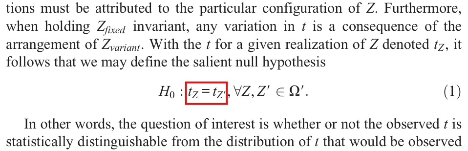
Equation (1) states the null hypothesis as equality of the test statistic over the assignments in Ω′\Omega'; the hypothesis that the procedure tests is equality of the fixed units' outcomes, under which the statistic still varies.

Equation (1) and the sentence that introduces it, p. 7 (PDF p. 5)

See also under Formal statements (Lean): P030-T5, P030-T6

As printed

With the tt for a given realization of ZZ denoted tZt_Z, it follows that we may define the salient null hypothesis

H0:tZ=tZ′, ∀Z,Z′∈Ω′.(1)H_0:\colorbox{#ffe58a}{$\displaystyle t_Z=t_{Z'}$},\ \forall Z,Z'\in\Omega'. \qquad (1)
The problem

The hypothesis of no interference, H0′′H_{0''} on p. 6, concerns outcomes: the outcome of a unit does not change when its own treatment does not. Since every assignment in Ω′\Omega' leaves the treatment of the fixed units unchanged, H0′′H_{0''} implies that YfixedY_{\mathit{fixed}} is the same for all Z∈Ω′Z\in\Omega'. It does not imply that the statistic is the same. The statistic tZt_Z depends on ZvariantZ_{\mathit{variant}} as well as on YfixedY_{\mathit{fixed}}, for example through DnearestD_{\mathit{nearest}}, and it can vary over Ω′\Omega' whether or not there is interference; the two sentences before the display say as much. Equation (1) does not follow from them, and it is not the hypothesis that the procedure tests. If Equation (1) held as printed, the reference distribution would be a point mass at the observed value and the pp value of Equation (2) would always equal 1. The article itself uses the hypothesis on outcomes. Table 1 lists three different values of the statistic under H0H_0, and p. 10 says that “in each randomization, we are assuming H0H_0, so YfixedY_{\mathit{fixed}} remains constant across randomizations”.

Evidence an exact counterexample

The evidence is a counterexample computed in exact arithmetic. I consider ten units at the positions 1,…,101,\ldots,10, of which one is treated, each with probability 1/101/10. Let the outcome of unit ii be bib_i under every assignment, where b=(1,2,2,2,2,3,2,3,2,1)b=(1,2,2,2,2,3,2,3,2,1). No outcome depends on any treatment, so there is no interference. Fix the units 1,8,9,101,8,9,10 and suppose that unit 7 is treated. Then Ω′\Omega' consists of the six assignments that treat one of the units 2,…,72,\ldots,7, each with conditional probability 1/61/6, and Yfixed=(1,3,2,1)Y_{\mathit{fixed}}=(1,3,2,1) under all six. The Spearman correlation between YfixedY_{\mathit{fixed}} and the distance to the treated unit is −1/90-1/\sqrt{90} when the treated unit is 2, 3 or 4, it is −5/6-5/6 when the treated unit is 5, and it is −3/10-3/\sqrt{10} when the treated unit is 6 or 7. These are the values −0.105-0.105, −0.833-0.833 and −0.949-0.949 of Table 1. Since 1/90≠25/361/90\ne 25/36, I have tZ≠tZ′t_Z\ne t_{Z'} for two assignments in Ω′\Omega', although the outcomes do not depend on the assignment. Counting the two assignments with tZ≤−3/10t_Z\le -3/\sqrt{10}, I obtain p=2/6p=2/6, which is the article’s 0.3330.333.

What survives

The correction adds no assumption and changes no number. The hypothesis H0′′H_{0''} and the conditioning on ZfixedZ_{\mathit{fixed}} are not affected, and Table 1 and p=0.333p=0.333 are already computed under the hypothesis on outcomes. The simulations and the application are described with a reference distribution that varies over the assignments, which agrees with the corrected hypothesis; their numbers were not recomputed for this correction.

Corrected

With the tt for a given realization of ZZ denoted tZt_Z, the salient null hypothesis is

H0:Yi,Z=Yi,Z′ for every i with Si=1, ∀Z,Z′∈Ω′.(1)H_0:\colorbox{#ffe58a}{$\displaystyle Y_{i,Z}=Y_{i,Z'}$}\ \colorbox{#ffe58a}{$\displaystyle \text{for every } i \text{ with } S_i=1$},\ \forall Z,Z'\in\Omega'. \qquad (1)

This hypothesis follows from H0′′H_{0''}, because every assignment in Ω′\Omega' leaves the treatment of the fixed units unchanged. Under H0H_0, the observed YfixedY_{\mathit{fixed}} is held constant and tZt_Z is recomputed for each Z∈Ω′Z\in\Omega'. The values tZt_Z need not be equal.

Four lines of text ending 'With the t for a given realization of Z denoted t_Z, it follows that we may define the salient null hypothesis', then the displayed Equation (1), 'H_0 : t_Z = t_Z-prime, for all Z, Z-prime in Omega-prime', then two further lines of text. A red box marks 't_Z = t_Z-prime' in the display.
Equation (1) with the sentence that introduces it, p. 7 (PDF p. 5). The equality tZ=tZ′t_Z=t_{Z'} is marked.
Table 1, titled 'Conditional Randomizations and Associated Test Statistics Under H_0', with columns Z, Y_fixed, D_nearest and rho_0 and six rows. Y_fixed is {1, 3, 2, 1} in every row. A red box marks the rho_0 column, whose entries are -0.105, -0.105, -0.105, -0.833, -0.949 and -0.949.
Table 1, p. 9 (PDF p. 7), whose title says that its statistics are computed under H0H_0. The column of ρ0\rho_0 is marked: it takes three different values over the six assignments in Ω′\Omega'.

The formula for the rank correlation lacks the square root in its denominator, and ρ\rho equals 11 or −1-1 under a strictly monotone relationship, not under every monotone one.

Practical Considerations, first paragraph, p. 8 (PDF p. 6): the formula for ρ\rho and the sentence after it

See also under Formal statements (Lean): P030-T8, P030-T9

As printed

Whenever values are tied, the average rank is used. ρ\rho then is the Pearson correlation coefficient of the ranks of these variables: ρ=cov⁡(rDnearest,rYfixed)/(var⁡(rDnearest)var⁡(rYfixed))\rho=\operatorname{cov}(r_{D_{\mathit{nearest}}},r_{Y_{\mathit{fixed}}})/\colorbox{#ffe58a}{$(\operatorname{var}(r_{D_{\mathit{nearest}}})\operatorname{var}(r_{Y_{\mathit{fixed}}}))$}. ρ\rho has a perfect correlation coefficient (of 1 or -1) whenever DnearestD_{\mathit{nearest}} has a monotone relationship with YfixedY_{\mathit{fixed}}.

The problem

The sentence names the Pearson correlation of the ranks, which divides the covariance by the square root of the product of the variances. The displayed expression divides by the product itself, and it is not a correlation. The next sentence is too broad when tied values are given average ranks. A relationship that is monotone but not strictly monotone can produce ties in one variable and not in the other, and then ∣ρ∣<1|\rho|<1.

Evidence a derivation

The evidence is a recalculation from Table 1 and a short derivation. In the last row of Table 1, the ranks of Dnearest=(6,1,2,3)D_{\mathit{nearest}}=(6,1,2,3) are (4,1,2,3)(4,1,2,3) and the ranks of Yfixed=(1,3,2,1)Y_{\mathit{fixed}}=(1,3,2,1) are (3/2,4,3,3/2)(3/2,4,3,3/2). With divisor nn, their covariance is −9/8-9/8 and their variances are 5/45/4 and 9/89/8. The printed expression gives (−9/8)/(45/32)=−4/5(-9/8)/(45/32)=-4/5, and −3/5-3/5 with divisor n−1n-1. The Pearson correlation is (−9/8)/45/32=−3/10(-9/8)/\sqrt{45/32}=-3/\sqrt{10}, which is the value −0.949-0.949 in the table. All six rows of Table 1 agree with the formula that has the square root.

For the second sentence, let D=(1,2,3)D=(1,2,3) and Y=(0,0,1)Y=(0,0,1), so that YY is a nondecreasing function of DD. The average ranks are (1,2,3)(1,2,3) and (3/2,3/2,3)(3/2,3/2,3), and ρ=3/2\rho=\sqrt{3}/2. The case of equality in the Cauchy–Schwarz inequality implies that ∣ρ∣=1|\rho|=1 exactly when the centered vectors of ranks are proportional.

What survives

Table 1, p=0.333p=0.333 and the test itself use the Pearson correlation of the ranks and do not change. I found no reported number from the simulations or the application that is shown to depend on the printed expression.

Corrected

Whenever values are tied, the average rank is used. ρ\rho then is the Pearson correlation coefficient of the ranks of these variables,

ρ=cov⁡(rDnearest,rYfixed)var⁡(rDnearest)var⁡(rYfixed),\rho=\frac{\operatorname{cov}(r_{D_{\mathit{nearest}}},r_{Y_{\mathit{fixed}}})}{\colorbox{#ffe58a}{$\displaystyle \sqrt{\operatorname{var}(r_{D_{\mathit{nearest}}})\operatorname{var}(r_{Y_{\mathit{fixed}}})}$}},

which is defined when neither vector of ranks is constant. ∣ρ∣=1|\rho|=1 exactly when the centered vectors of ranks are proportional. This holds whenever DnearestD_{\mathit{nearest}} has a strictly monotone relationship with YfixedY_{\mathit{fixed}}, under which ties in one variable correspond to ties in the other. A relationship that is monotone but not strictly monotone need not give ∣ρ∣=1|\rho|=1.

Five lines of text. In the third line a red box marks the denominator '(var(r_D_nearest) var(r_Y_fixed))' of the formula 'rho = cov(r_D_nearest, r_Y_fixed) / (var(r_D_nearest) var(r_Y_fixed))'. In the fourth line a second red box marks the word 'monotone' in 'whenever D_nearest has a monotone relationship with Y_fixed'.
Practical Considerations, first paragraph, p. 8 (PDF p. 6). The denominator of the formula for ρ\rho and the word “monotone” are marked.

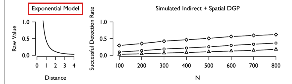
The third simulated model is an inverse-square decay, not an exponential one, and its sums should exclude the term j=ij=i.

Simulation Studies, the third distance-decay model, p. 10 (PDF p. 8); the name recurs on p. 11 (PDF p. 9) and in Figure 2, p. 12 (PDF p. 10)

See also under Formal statements (Lean): P030-T10

As printed

The third model is an exponential model, for which Θi=∑j((1−δij)Zj/((1.5dij)2))\Theta_i=\colorbox{#ffe58a}{${\textstyle\sum_j}$}\bigl((1-\delta_{ij})Z_j/((1.5d_{ij})^2)\bigr) and Ψi=∑j((1−δij)/((1.5dij)2))\Psi_i=\colorbox{#ffe58a}{${\textstyle\sum_j}$}\bigl((1-\delta_{ij})/((1.5d_{ij})^2)\bigr). In the exponential model, the effect asymptotically approaches ∞\infty as dijd_{ij} approaches zero. In all cases, both Θ\Theta and Ψ\Psi are mean-normalized to one.

The problem

For d>0d>0 the decay function is 1/(1.5d)2=4/(9d2)1/(1.5d)^2=4/(9d^2), a power of the distance. It falls by a factor of 4 whenever the distance doubles, and it diverges as d→0d\to 0, as the article notes. An exponential decay exp⁡(−cd)\exp(-cd) is bounded at d=0d=0 and falls by a constant factor for each unit of distance. The model is called exponential on pp. 10 and 11 and in the title of the lower-left panel of Figure 2. As described, the simulations do not include an exponential decay. Separately, the sums run over all jj. For j=ij=i the summand is (1−δii)/(1.5dii)2=0/0(1-\delta_{ii})/(1.5d_{ii})^2=0/0, which the factor 1−δij1-\delta_{ij} does not define; the sums meant are over j≠ij\ne i.

Evidence a derivation

The evidence is a derivation from the printed formula and a check of the pages. Let k(d)=4/(9d2)k(d)=4/(9d^2). Then k(2d)/k(d)=1/4k(2d)/k(d)=1/4 for every d>0d>0, and the derivative of log⁡k(d)\log k(d) is −2/d-2/d, which is not constant as it is for an exponential decay. The curve in the lower-left panel of Figure 2 agrees with k(2/3)=1k(2/3)=1, k(1)=4/9k(1)=4/9 and k(2)=1/9k(2)=1/9. The page prints no restriction to j≠ij\ne i.

What survives

The formula and the plotted curve agree on the decay function, and no reported detection rate is shown to change. The simulation code is not available. The correction concerns the name and the notation, and it is not a check of the implementation. The simulations cover Gaussian, linear and inverse-square decay; they do not show how the method behaves under exponential decay.

Corrected

The third model is an inverse-square model, for which

Θi=∑j≠iZj/(1.5dij)2andΨi=∑j≠i1/(1.5dij)2.\Theta_i=\colorbox{#ffe58a}{$\displaystyle \sum_{j\ne i}$}Z_j/(1.5d_{ij})^2 \quad\text{and}\quad \Psi_i=\colorbox{#ffe58a}{$\displaystyle \sum_{j\ne i}$}1/(1.5d_{ij})^2 .

In the inverse-square model, the effect asymptotically approaches ∞\infty as dijd_{ij} approaches zero. In all cases, both Θ\Theta and Ψ\Psi are mean-normalized to one.

The same name replaces “exponential” on p. 11 (“DGPs with the exponential model”) and in Figure 2 (“Exponential Model”).

Five lines of text. In the first line a red box marks the word 'exponential' in 'The third model is an exponential model'. In the second line a second red box marks the formula 'sum over j of ((1 - delta_ij) Z_j / ((1.5 d_ij)^2))' that defines Theta_i. The next sentence reads 'In the exponential model, the effect asymptotically approaches infinity as d_ij approaches zero.'
Simulation Studies, p. 10 (PDF p. 8): the definition of the third distance-decay model. The word “exponential” and the sum that defines Θi\Theta_i are marked.
The lower row of Figure 2. At the left, a panel titled 'Exponential Model', marked with a red box, plots 'Raw Value' against 'Distance' from 0 to 4: a curve that leaves the top of the panel near distance 0.7 and falls towards zero. At the right, a panel titled 'Simulated Indirect + Spatial DGP' plots 'Successful Detection Rate' against N from 100 to 800 for three significance levels.
Figure 2, p. 12 (PDF p. 10), lower panels. The title “Exponential Model” is marked; the curve below it is 1/(1.5d)21/(1.5d)^2.

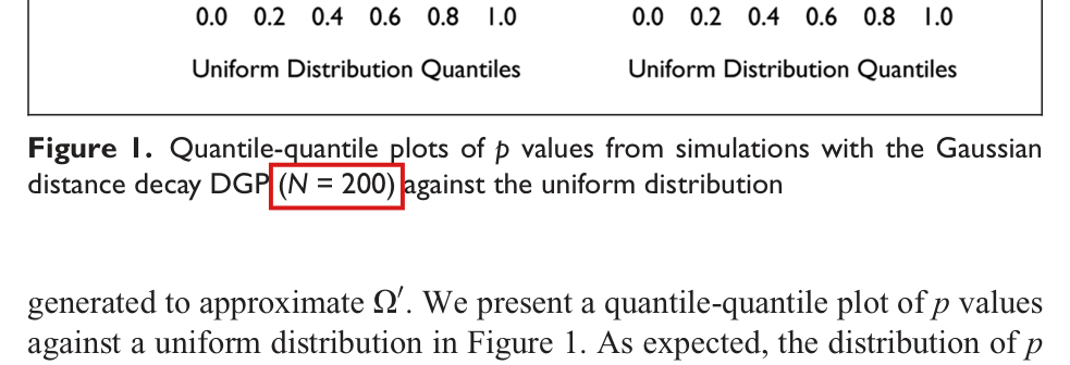
The text states N=400N = 400 for the simulation shown in Figure 1 and the caption states N=200N = 200; one of the two numbers is wrong.

Figure 1 caption, p. 11 (PDF p. 9); the simulation it belongs to is described at the foot of p. 10 (PDF p. 8)

As printed

Page 10, text: “First, we illustrate a set of results for a simulation study using the Gaussian model, where N=400N = \colorbox{#ffe58a}{$400$}, 200 units are randomly assigned to treatment, and 200 units are assigned to control. For all simulations, we choose the fixed subset as a random sample of control units; following the rule of thumb, Nfixed=100N_{\mathit{fixed}} = 100.”

Page 11, caption: “Figure 1. Quantile-quantile plots of pp values from simulations with the Gaussian distance decay DGP (N=200N = \colorbox{#ffe58a}{$200$}) against the uniform distribution”

The problem

In the paper NN is the total number of units (p. 5). The text introduces Figure 1 with N=400N = 400, of which 200 units are treated and 200 are controls, and the caption of the same figure states N=200N = 200.

Evidence a check of the printed page

A check of the two pages. The simulation code and its output are not available, and the two pages do not settle which sample size produced the plot.

What survives

Only the sample size attributed to Figure 1 is in doubt. The plot, the 83% rejection rate and the Kolmogorov–Smirnov p=0.661p = 0.661 are not shown to be wrong.

Corrected

The two descriptions are to be reconciled with the original simulation output. If the design in the text produced the figure, the caption reads “… with the Gaussian distance decay DGP (N=400N = \colorbox{#ffe58a}{$400$}) against the uniform distribution”. If a simulation with N=200N = 200 produced it, the text needs the counts of that simulation instead: under the same rule of thumb, 100 treated units, 100 control units and Nfixed=50N_{\mathit{fixed}} = 50. Without that output, neither number is relabelled.

The foot of Figure 1, with the axis label Uniform Distribution Quantiles under each of its two panels, then the caption: Figure 1. Quantile-quantile plots of p values from simulations with the Gaussian distance decay DGP (N = 200) against the uniform distribution. A red box marks '(N = 200)'. Two lines of the next paragraph are visible below.
Caption of Figure 1, p. 11 (PDF p. 9): the sample size “(N=200N = 200)” is marked.
Five lines of text beginning 'First, we illustrate a set of results for a simulation study using the Gaussian model, where N = 400, 200 units are randomly assigned to treatment, and 200 units are assigned to control'. A red box marks 'N = 400,'. The last line gives N_fixed = 100.
Last paragraph of p. 10 (PDF p. 8): the text introduces the same simulation with “N=400N = 400”, which is marked.

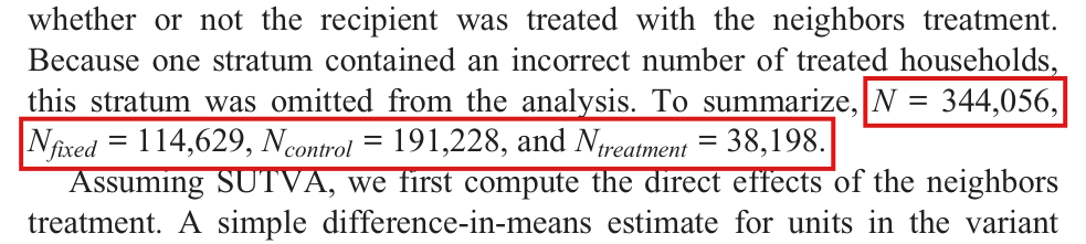
The three group counts sum to 344,055, one fewer than the printed N=344,056N = 344{,}056.

Application, p. 13 (PDF p. 11), the sentence that begins “To summarize”

See also under Formal statements (Lean): P030-T11

As printed

To summarize, N=344,056N = \colorbox{#ffe58a}{$344{,}056$}, Nfixed=114,629N_{\mathit{fixed}} = \colorbox{#ffe58a}{$114{,}629$}, Ncontrol=191,228N_{\mathit{control}} = \colorbox{#ffe58a}{$191{,}228$}, and Ntreatment=38,198N_{\mathit{treatment}} = \colorbox{#ffe58a}{$38{,}198$}.

The problem

The fixed, control and treatment groups are disjoint and together make up the analysis sample, so their counts sum to NN. A direct computation gives 114,629+191,228+38,198=344,055114{,}629 + 191{,}228 + 38{,}198 = 344{,}055. The counts are inconsistent by one; the arithmetic does not identify which entries are wrong.

Evidence an exact counterexample

An exact calculation with the printed counts. The log of the source study records 344,084 voters before the stratum was omitted: 114,640 in the three fixed conditions, 191,243 in control and 38,201 in the neighbors condition. Then the printed NN implies that 28 voters were omitted, and the printed group counts imply 29. I did not examine the voter-level data, and the omitted stratum and the incorrect counts are not identified.

What survives

The method and the simulations do not use these counts. The discrepancy alone does not show that the estimate of the direct effect, the rank correlation, Figure 3 or the pp value rests on a wrong sample. I did not recompute those, since the distances and the analysis code are not available.

Corrected

The counts are to be reconciled with the analysis sample. If the total, the control count and the treatment count are kept, the sentence reads: “To summarize, N=344,056N = 344{,}056, Nfixed=114,630N_{\mathit{fixed}} = \colorbox{#ffe58a}{$114{,}630$}, Ncontrol=191,228N_{\mathit{control}} = 191{,}228, and Ntreatment=38,198N_{\mathit{treatment}} = 38{,}198.” The sum is also restored if any one of the other three entries is changed by one unit: N=344,055N = 344{,}055, Ncontrol=191,229N_{\mathit{control}} = 191{,}229 or Ntreatment=38,199N_{\mathit{treatment}} = 38{,}199.

Six lines of text. Red boxes mark 'N = 344,056,' at the end of one line and 'N_fixed = 114,629, N_control = 191,228, and N_treatment = 38,198.' on the next line.
Application, p. 13 (PDF p. 11): the four counts in the sentence that begins “To summarize” are marked.

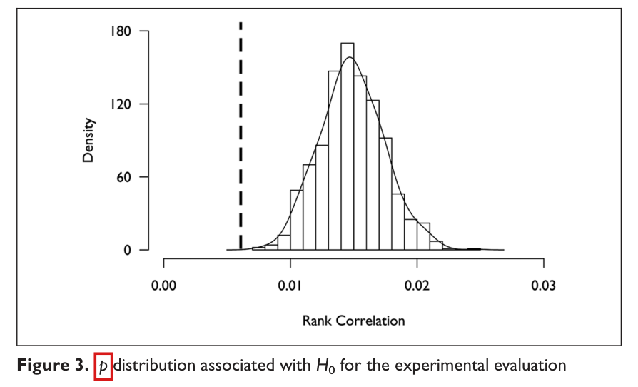
The caption of Figure 3 prints pp where ρ0\rho_0 is meant: the figure shows the distribution of the rank correlation under H0H_0.

Figure 3 caption, p. 14 (PDF p. 12)

As printed

Figure 3. p\colorbox{#ffe58a}{$p$} distribution associated with H0H_0 for the experimental evaluation

The problem

The figure is a histogram of the rank correlation under the null hypothesis. Its horizontal axis is labelled “Rank Correlation”, and p. 13 introduces it as “T0T_0, the approximate distribution of ρ0\rho_0 associated with H0H_0”. The symbol in the caption is the italic pp that the caption of Figure 1 uses for pp values.

Evidence a check of the printed page

A check of the page: the caption, the axis label and the sentence on p. 13.

What survives

Only the symbol in the caption changes. The histogram and the results drawn from it are unaffected.

Corrected

Figure 3. ρ0\colorbox{#ffe58a}{$\rho_0$} distribution associated with H0H_0 for the experimental evaluation

Figure 3: a histogram with a smooth curve over it, centred near 0.015 on a horizontal axis labelled Rank Correlation that runs from 0.00 to 0.03, with a dashed vertical line near 0.006. The vertical axis is labelled Density. Below, the caption reads: Figure 3. p distribution associated with H0 for the experimental evaluation. A red box marks the letter p.
Figure 3 and its caption, p. 14 (PDF p. 12): the symbol pp in the caption is marked. The horizontal axis reads “Rank Correlation”.

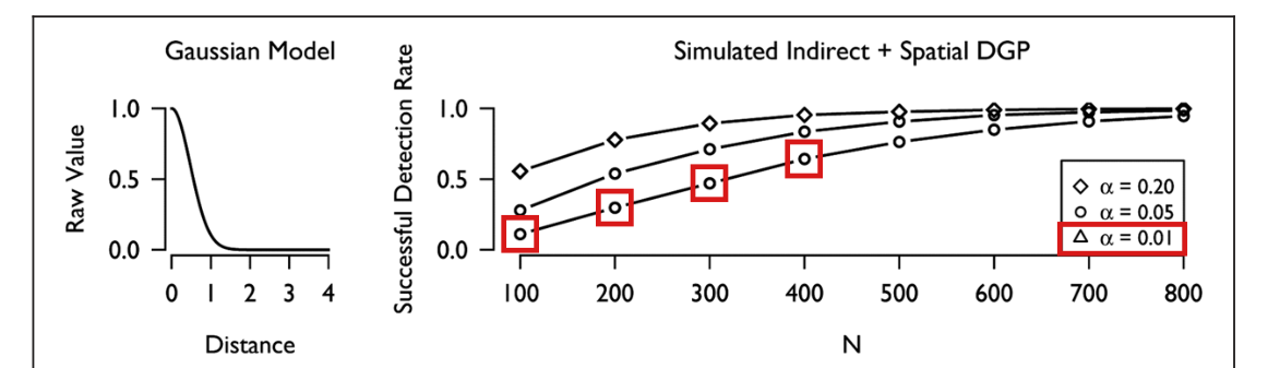
In the Gaussian panel of Figure 2 the α=0.01\alpha = 0.01 curve is drawn with circles, the marker that the legend assigns to α=0.05\alpha = 0.05; it should carry triangles.

Figure 2, Gaussian model panel (top right) and its legend, p. 12 (PDF p. 10)

As printed

A figure, described. The legend in the Gaussian panel assigns a diamond to α=0.20\alpha = 0.20, a circle to α=0.05\alpha = 0.05 and a triangle to α=0.01\alpha = 0.01. In that panel the top curve has diamonds, the middle curve has circles and the lowest curve has circles. In the linear and exponential panels the lowest curve has triangles.

The problem

Two curves in the Gaussian panel carry the same marker, and the legend does not identify the lowest one. Its position does. Since the test rejects less often at a smaller α\alpha, the lowest curve is the α=0.01\alpha = 0.01 series.

Evidence a check of the printed page

A check of the page. Enlarged, the markers of the lowest Gaussian curve at N=100N = 100 to 400400, where the curves are separated, are circles.

What survives

Only the marker is wrong. No plotted value is shown to be wrong, and nothing else in the paper depends on it.

Corrected

Draw the Gaussian α=0.01\alpha = 0.01 curve with open triangles, as the legend has it, and keep open circles for α=0.05\alpha = 0.05.

The top row of Figure 2: a small plot of the Gaussian kernel against distance, and a plot of successful detection rate against N from 100 to 800 with three rising curves. The top curve has diamonds; the middle and lowest curves both have open circles. Red boxes mark the four circles of the lowest curve at N = 100, 200, 300 and 400, and the legend line that shows an open triangle for alpha = 0.01.
Figure 2, Gaussian model row, p. 12 (PDF p. 10): the markers of the lowest curve at N=100N = 100 to 400400 and the legend entry for α=0.01\alpha = 0.01 are marked.

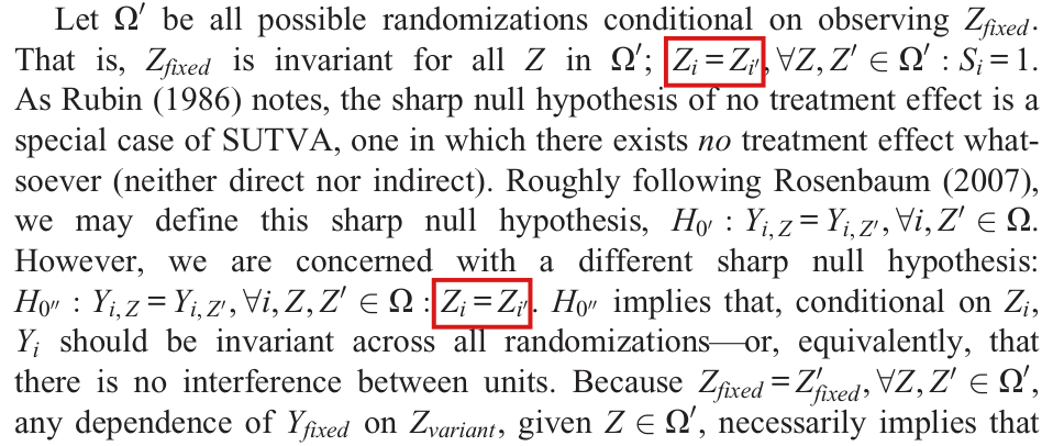
In the definition of Ω′\Omega' and in H0′′H_{0''} the prime is printed on the unit index, Zi=Zi′Z_i=Z_{i'}, where Zi=Zi′Z_i=Z'_i is meant.

Method, second paragraph, p. 6 (PDF p. 4): the definition of Ω′\Omega' and the statement of H0′′H_{0''}

See also under Formal statements (Lean): P030-T7, P030-T12

As printed

Let Ω′\Omega' be all possible randomizations conditional on observing ZfixedZ_{\mathit{fixed}}. That is, ZfixedZ_{\mathit{fixed}} is invariant for all ZZ in Ω′\Omega'; Zi=Zi′Z_i=\colorbox{#ffe58a}{$Z_{i'}$}, ∀Z,Z′∈Ω′:Si=1\forall Z,Z'\in\Omega':S_i=1. … However, we are concerned with a different sharp null hypothesis: H0′′:Yi,Z=Yi,Z′, ∀i,Z,Z′∈Ω:Zi=Zi′H_{0''}:Y_{i,Z}=Y_{i,Z'},\ \forall i,Z,Z'\in\Omega:Z_i=\colorbox{#ffe58a}{$Z_{i'}$}.

The problem

As printed, each condition compares the treatment of unit ii with the treatment of a unit i′i' in the same vector ZZ, and no unit i′i' is defined. The condition meant is that unit ii has the same treatment under the two assignments ZZ and Z′Z'.

Evidence a check of the printed page

The evidence is a check of the page. The units are indexed by i∈{1,2,…,N}i\in\{1,2,\ldots,N\} on p. 4, and no index i′i' is introduced. Two lines below the statement of H0′′H_{0''}, the same condition for the fixed subset is printed with the prime on the vector: Zfixed=Zfixed′Z_{\mathit{fixed}}=Z'_{\mathit{fixed}}, ∀Z,Z′∈Ω′\forall Z,Z'\in\Omega'.

What survives

Nothing depends on the misprint. The article uses Ω′\Omega' and H0′′H_{0''} in their intended form in everything that follows.

Corrected

Let Ω′\Omega' be all possible randomizations conditional on observing ZfixedZ_{\mathit{fixed}}. That is, ZfixedZ_{\mathit{fixed}} is invariant for all ZZ in Ω′\Omega'; Zi=Zi′Z_i=\colorbox{#ffe58a}{$Z'_i$}, ∀Z,Z′∈Ω′:Si=1\forall Z,Z'\in\Omega':S_i=1. … H0′′:Yi,Z=Yi,Z′, ∀i,Z,Z′∈Ω:Zi=Zi′H_{0''}:Y_{i,Z}=Y_{i,Z'},\ \forall i,Z,Z'\in\Omega:Z_i=\colorbox{#ffe58a}{$Z'_i$}.

Eleven lines of text from the Method section. Red boxes mark the expression 'Z_i = Z_i-prime', with the prime on the subscript i, in the second line (the definition of Omega-prime) and in the eighth line (the statement of the null hypothesis H_0''). Two lines below the second box the text reads 'Because Z_fixed = Z-prime_fixed, for all Z, Z-prime in Omega-prime', with the prime on Z.
Method, second paragraph, p. 6 (PDF p. 4). The two conditions Zi=Zi′Z_i=Z_{i'} are marked; two lines below the second mark, the same condition is printed correctly for the fixed subset, as Zfixed=Zfixed′Z_{\mathit{fixed}}=Z'_{\mathit{fixed}}.

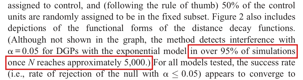
With the two-tailed test of the surrounding text, a recalculation detects interference under the third model in 93.0% of simulations at N=5,000N = 5{,}000 and 92.25% at N=6,000N = 6{,}000, not in over 95%.

Simulation Studies, p. 11 (PDF p. 9), the parenthetical that follows the description of Figure 2

As printed

(Although not shown in the graph, the method detects interference with α=0.05\alpha = 0.05 for DGPs with the exponential model in over 95% of simulations once NN reaches approximately 5,000.)

The problem

The sentence concerns the third model, which the paper calls exponential and whose kernel is the inverse square 1/(1.5dij)21/(1.5 d_{ij})^2 (see P030-E006). It does not say whether its test is one-tailed or two-tailed, and “approximately 5,000” has no stated tolerance. Since the paragraph before it reports a rejection rate “when using a two-tailed test”, the natural reading is the two-tailed rule of p. 7 at α=0.05\alpha = 0.05.

Under that reading the stated rate is too high. In a recalculation of the design as printed, the two-tailed test detects interference in 93.0% of simulations at N=5,000N = 5{,}000 and in 92.25% at N=6,000N = 6{,}000. With the one-tailed pp value of Equation (2), the rates are 94.83% and 94.5%, which neither bear out “over 95%” nor contradict it. At N=8,000N = 8{,}000 the estimate of the two-tailed rate is 97.00%.

Evidence a simulation

A recalculation by simulation of the design printed on pp. 10–11. Each unit has coordinates drawn uniformly on [0,N]2[0, \sqrt{N}]^2 and noise ϵi∼N(0,1)\epsilon_i \sim N(0,1). The outcome is

Yi=Zi+Θi+Ψi+ϵi,Θi=∑j≠iZj(1.5dij)2,Ψi=∑j≠i1(1.5dij)2,Y_i = Z_i + \Theta_i + \Psi_i + \epsilon_i, \qquad \Theta_i = \sum_{j \neq i} \frac{Z_j}{(1.5 d_{ij})^2}, \qquad \Psi_i = \sum_{j \neq i} \frac{1}{(1.5 d_{ij})^2},

where Θ\Theta and Ψ\Psi are each divided by their mean over the NN units. Half of the units are treated, and a random half of the controls is the fixed subset. The statistic is the rank correlation between YfixedY_{\mathit{fixed}} and the distance to the nearest treated unit, and each simulation uses 5,000 conditional randomizations, the number that the paper reports for Figure 1. The one-tailed test rejects when the pp value of Equation (2) is below 0.05. The two-tailed test rejects when it is below 0.025 or above 0.975.

Third model, α=0.05\alpha = 0.05: rejections among the simulations, with the rate and its Monte Carlo standard error in percentage points.
NNSimulationsTwo-tailedRate (s.e.)One-tailedRate (s.e.)
5,00060055893.00% (1.04)56994.83% (0.90)
6,00040036992.25% (1.34)37894.50% (1.14)
8,00030029197.00% (0.98)29297.33% (0.93)

At N=5,000N = 5{,}000 and N=6,000N = 6{,}000 the exact 95% intervals for the two-tailed rate are [0.907,0.949][0.907, 0.949] and [0.892,0.947][0.892, 0.947], and both end below 0.95. Testing the two counts together, 927 rejections in 1,000 simulations, with an exact binomial test against a rate of at least 0.95 at both values of NN, I find p=0.001p = 0.001. The one-tailed intervals, [0.927,0.965][0.927, 0.965] and [0.918,0.965][0.918, 0.965], contain 0.95. I checked the code against an exhaustive enumeration of the 84 conditional assignments of a small example.

The original simulation code and output are not available. The rates above are estimates from this recalculation, with the Monte Carlo error stated, and three values of NN do not establish the rate at every larger NN.

What survives

The method, the worked example, the Gaussian result and the plotted curves of Figure 2 do not depend on this sentence. The application reports p<0.001p < 0.001, which rejects under either tail rule. Only the sentence itself changes: near N=5,000N = 5{,}000 the detection rate of the two-tailed test under this model is about 93%, and the one-tailed rate is not shown to exceed 95%.

Corrected

(Although not shown in the graph, for DGPs with the inverse-square model and α=0.05\alpha = 0.05, a recalculation with 5,000 conditional randomizations per simulation detects interference with the two-tailed test in 93.0% of 600 simulations at N=5,000N = 5{,}000 and 92.25% of 400 simulations at N=6,000N = 6{,}000 (standard errors 1.04 and 1.34 percentage points). With the one-tailed pp value of Equation (2), the rates are 94.83% and 94.5% (standard errors 0.90 and 1.14). At N=8,000N = 8{,}000, in 300 simulations, the rates are 97.00% two-tailed and 97.33% one-tailed (standard errors 0.98 and 0.93).)

These rates are for the design of pp. 10–11: the kernel 1/(1.5dij)21/(1.5 d_{ij})^2 summed over j≠ij \neq i, Θ\Theta and Ψ\Psi each normalized to mean one, half of the units treated, and a random half of the controls fixed. The words “over 95% of simulations once NN reaches approximately 5,000” are not kept. If the sentence is restated for the one-tailed test, they are still not supported, since the one-tailed rates at N=5,000N = 5{,}000 and 6,0006{,}000 are not shown to exceed 95%.

Seven lines of text. Red boxes mark the words 'in over 95 percent of simulations' at the end of one line and 'once N reaches approximately 5,000.)' at the start of the next, inside the sentence '(Although not shown in the graph, the method detects interference with alpha = 0.05 for DGPs with the exponential model in over 95 percent of simulations once N reaches approximately 5,000.)'.
Simulation Studies, p. 11 (PDF p. 9): the parenthetical on detection at large NN, with “in over 95% of simulations once NN reaches approximately 5,000.)” marked.

Clarity notes

Imprecise or ambiguous wording whose intended meaning is correct; not an error.

The numerator of Equation (2) is the number of assignments in Ω′\Omega' whose statistic is at most the observed one; assignments with equal statistics are each counted.

Equation (2), the numerator, p. 7 (PDF p. 5)

As printed

p=Pr⁡(t0≤t)=∣{t0∈T0:t0≤t}∣/∣Ω′∣.(2)p=\Pr(t_0\le t)=\colorbox{#ffe58a}{$\displaystyle |\{t_0\in T_0:t_0\le t\}|$}/|\Omega'|. \qquad (2)

Intended meaning

The numerator is written as the size of a set of values of the statistic, and a set in the usual sense does not repeat equal values. The count meant is over assignments. The paragraph before the display builds T0T_0 from one t0t_0 for each Z∈Ω′Z\in\Omega' and calls it a distribution, and the worked example counts “2 of the 6 conditional randomizations” on p. 10, although the six assignments of Table 1 have only three distinct values of ρ0\rho_0. Read in this way, the display is the lower-tail probability, and I obtain the article’s p=2/6=0.333p=2/6=0.333. Counting distinct values would give 1/61/6.

Corrected

p=Pr⁡(t0≤t)=∣{Z∈Ω′:t0(Z)≤t}∣/∣Ω′∣,(2)p=\Pr(t_0\le t)=\colorbox{#ffe58a}{$\displaystyle |\{Z\in\Omega':t_0(Z)\le t\}|$}/|\Omega'|, \qquad (2)

where t0(Z)t_0(Z) denotes the statistic computed under H0H_0 for the assignment ZZ.

Four lines of text ending 'and assuming that all Z in Omega-prime occur with equal probability,', followed by the displayed Equation (2). A red box marks the numerator '|{t_0 in T_0 : t_0 <= t}|'.
Equation (2) with the sentences that introduce it, p. 7 (PDF p. 5). The numerator is marked.

The symbol “!∃ρ0!\exists\rho_0” means that each assignment in Ω′\Omega' has exactly one value ρ0\rho_0; the usual symbol is ∃!\exists!.

A Simple Example, second paragraph, p. 9 (PDF p. 7)

As printed

And for each Z∈Ω′Z\in\Omega', !∃ρ0\colorbox{#ffe58a}{$!\exists$}\rho_0, the rank correlation under H0H_0.

Intended meaning

The exclamation mark is printed before the existential quantifier. This is not the usual order for the symbol of unique existence, and the mark could be taken for a negation. The article defines no such convention, and Table 1 lists one ρ0\rho_0 for each of the six assignments. The sentence means that each Z∈Ω′Z\in\Omega' determines exactly one rank correlation under H0H_0, and nothing false is printed.

Corrected

And for each Z∈Ω′Z\in\Omega', there exists a unique ρ0\rho_0, the rank correlation under H0H_0.

Four lines of text. In the third line a red box marks an exclamation mark followed by the existential quantifier, in the sentence 'And for each Z in Omega-prime, ! exists rho_0, the rank correlation under H_0.'
A Simple Example, second paragraph, p. 9 (PDF p. 7). The symbol !∃!\exists is marked.

Formal statements (Lean)

Formal results: 14 whole; 0 restricted; 1 refuted; 0 omitted.

Coverage concerns the identified claim under its stated assumptions. A checked proof establishes the formal statement; correspondence to the published text was reviewed by AI. Repository access is currently required to open the source links.

Each result links to its current formal statement and proof. “Whole” covers the identified claim under its assumptions; “restricted” covers the stated narrower scope; “refuted” gives a counterexample to the identified assertion; “omitted” has no current theorem. Any named published theorem used as a premise remains an assumption. Browse the formal results for this work.

Two-tailed rule after Equation (2), with 'This procedure is an exact, distribution-free test', as printed: a five-unit experiment without interference in which the rule rejects with probability 1

p. 7 (PDF p. 5)

p. 7 (PDF p. 5): the five-unit experiment has no effects, defined Spearman statistics equal to one, printed rejection probability one, and corrected rejection probability zero, with the stated distances and rank computations.

Historical component credits
  • Proved AronowAudit.P030.five_no_effects Historical support retained; baseline fidelity: ok; manifest: used; used in Solution; The no-effect component is already exported by five_unit_counterexample.
  • Proved AronowAudit.P030.five_distances Historical support retained; baseline fidelity: ok; manifest: used; used in Solution; The treated-variant set is a singleton in both cases; the empty-set nearest-distance branch is unused.
  • Proved AronowAudit.P030.five_correlations Limited support; baseline fidelity: narrower; manifest: used; used in Solution; {'source': 'adjudication+second review', 'adjudicator': "At P030/P030_Audit.lean:195-197, five_correlations concludes only that each distance rank-square sum is 2, the outcome rank-square sum is 2, and fiveStatistic is 1. T1's computation and this row explicitly assert that the outcome and both distance rank vectors are (1,2,3), but neither averageRank vector equality is in this declaration's conclusion. The aggregate sums and correlation do not state those pointwise rank identities; five_rank_certificate at P030/P030_Audit.lean:1810-1813 separately states them, preserving the theorem family's coverage without satisfying this row's credited conclusion. The definitions match the specified experiment and the positive square sums ensure a defined correlation, so the defect is precisely the omitted rank-vector conclusions.", 'suggested_fix': 'Extend five_correlations with the conjuncts averageRank fiveOutcomes = ![1,2,3] and (∀ a : Fin 2, averageRank (fiveDistances a) = ![1,2,3]), retaining its existing sums-of-squares and correlation conclusions. These are already stated in five_rank_certificate.', 'second_review': "At P030/P030_Audit.lean:195, five_correlations exports only rank-square sums of 2 and correlations of 1. T1 expressly says that the outcome and both distance vectors have ranks '(1, 2, 3)', so those conclusions belong to this row's credited component and are missing. The omission is minor: evaluating averageRank (P030/P030_Audit.lean:116) on these explicitly specified three-entry vectors requires only finite comparison and counting. Add the rank-vector conjuncts already separately stated by five_rank_certificate (P030/P030_Audit.lean:1810).", 'severity': 'minor'}
  • Proved AronowAudit.P030.five_design Historical support retained; baseline fidelity: ok; manifest: used; used in Solution; All design components are already exported by five_unit_counterexample; no separate invocation is needed.
  • Counterexample proved AronowAudit.P030.five_unit_counterexample Historical support retained; baseline fidelity: ok; manifest: used; used in Solution; The repeated alpha<1 conclusion is redundant and does not affect fidelity; constant correlation across assignments does not mean either ranked input vector is constant.
  • Proved AronowAudit.P030.five_rank_certificate Historical support retained; baseline fidelity: ok; manifest: used; used in Solution; This separate declaration supplies the explicit rank certificates missing from R196-01.

Two-tailed rule after Equation (2), as printed: under the reference law of the paper's own Table 1, realized in a population without interference, the rule rejects with probability 1/2

p. 7 (PDF p. 5); Table 1 and the example on p. 9 (PDF p. 7)

p. 7 and Table 1, p. 9 (PDF pp. 5, 7): a genuine no-effects ten-unit population realizes the table's six-assignment conditional law. All midranks, centered ranks, products, square sums, squared correlations, strict orders, roundings, and inclusive tails have their stated values. For 0 < alpha <= 2/3 the printed rule rejects exactly the three assignments with p = 1 and has conditional size 1/2; the corrected rule rejects none. The printed size exceeds every positive alpha < 1/2, including alpha = 1/20.

Historical component credits
  • Proved AronowAudit.P030.table_tail_probabilities Historical support retained; baseline fidelity: ok; manifest: used; used in Solution; Inclusive inequalities and all tied assignments are counted; no distinct-value collapse occurs.
  • Proved AronowAudit.P030.table_rejection_probabilities Historical support retained; baseline fidelity: ok; manifest: used; used in Solution; Use ten_actual_conditional_size, which connects these row-indexed sizes directly to the actual conditional experiment.
  • Counterexample proved AronowAudit.P030.ten_unit_counterexample Historical support retained; baseline fidelity: ok; manifest: not used; not used in Solution; The null population is deliberately different from the paper's interfering illustrative DGP, as required by the target.
  • Proved AronowAudit.P030.ten_null_statistic_value Historical support retained; baseline fidelity: ok; manifest: used; used in Solution; This is a supporting statistic identity for the null witness, rather than a proof of the printed positive claim.
  • Proved AronowAudit.P030.ten_null_reference_value Historical support retained; baseline fidelity: ok; manifest: used; used in Solution; The observed and reference row quantifiers vary independently, so no assignment is omitted.
  • Proved AronowAudit.P030.ten_actual_conditional_size Historical support retained; baseline fidelity: ok; manifest: used; used in Solution; This row supplies the direct observed-data/statistic connection that an abstract row-index calculation alone would leave implicit.

Two-tailed rule after Equation (2), corrected: reject when either inclusive tail probability is below α/2\alpha/2 (with the proof of its level)

p. 7 (PDF p. 5)

p. 7 (PDF p. 5), corrected: the two-inclusive-tail rule controls size for every finite probability law, with the tail identity, super-uniformity, union bound, printed-rule inclusion, genuine strictness example, and conventional alternative.

Historical component credits
  • Proved AronowAudit.P030.probability_nonneg Historical support retained; baseline fidelity: ok; manifest: used; used in Solution; Nonnegativity of the law’s individual masses is part of being a probability law, not an added assumption about the statistic.
  • Proved AronowAudit.P030.probability_mono Historical support retained; baseline fidelity: ok; manifest: used; used in Solution; Supportwise inclusion is the relevant event inclusion because masses outside the finite support are ignored.
  • Proved AronowAudit.P030.probability_true Historical support retained; baseline fidelity: ok; manifest: not used; not used in Solution; Normalization is already part of FiniteLaw and the selected validity results.
  • Proved AronowAudit.P030.probability_le_one Historical support retained; baseline fidelity: ok; manifest: not used; not used in Solution; A helper bound not needed separately for any stated clause.
  • Proved AronowAudit.P030.tail_identity Historical support retained; baseline fidelity: ok; manifest: used; used in Solution; Keeping the atom term is essential for ties and matches the correction; its nonnegativity also yields the target’s pU≥1−pL consequence.
  • Proved AronowAudit.P030.lowerTail_mono Historical support retained; baseline fidelity: ok; manifest: not used; not used in Solution; Auxiliary monotonicity is already absorbed into the exported lower-tail validity result.
  • Proved AronowAudit.P030.lower_tail_valid Historical support retained; baseline fidelity: ok; manifest: used; used in Solution; The extension above one is harmless since event probabilities are at most one; no target case is excluded.
  • Proved AronowAudit.P030.upper_tail_valid Historical support retained; baseline fidelity: ok; manifest: used; used in Solution; The extension above one is harmless since event probabilities are at most one; no target case is excluded.
  • Proved AronowAudit.P030.probability_union_le Historical support retained; baseline fidelity: ok; manifest: used; used in Solution; An auxiliary bound for arbitrary events, applied in the target to the two inclusive-tail events.
  • Proved AronowAudit.P030.corrected_two_tailed_valid Historical support retained; baseline fidelity: ok; manifest: used; used in Solution; Proves the corrected strict rule’s level, not validity of the faulty printed rule. Matching the same finite law in observed and reference statistics is exactly the target’s formal setup.
  • Proved AronowAudit.P030.corrected_reject_subset_printed Historical support retained; baseline fidelity: ok; manifest: used; used in Solution; Proves only the described inclusion implication; it does not claim to export the strict-inclusion witness mentioned elsewhere in target part (v).
  • Proved AronowAudit.P030.twoTailP_event Historical support retained; baseline fidelity: ok; manifest: used; used in Solution; The algebraic generalization preserves the intended p-value specialization and the inclusive boundary.
  • Proved AronowAudit.P030.conventional_two_tailed_valid Historical support retained; baseline fidelity: ok; manifest: used; used in Solution; Proves the conventional alternative’s level guarantee in T3(vi), not the printed test’s level guarantee.

Equation (2) and the two-tailed rule ('This procedure is an exact, distribution-free test for detecting interference between units'), as printed

p. 7 (PDF p. 5)

The printed claim is false: P030-T4, p. 7 (PDF p. 5), the printed two-tailed rule does not universally control conditional Type I error under no interference.

Historical component credits
  • Counterexample proved AronowAudit.P030.printed_two_tailed_claim_false Historical support retained; baseline fidelity: ok; manifest: used; used in Solution; This is a full refutation, not positive exactness: nonempty conditioning fibers always contain a supported assignment with the same fixed-treatment pattern, so allowing an unsupported a changes no fiber. The target itself quantifies over statistic choices; the supplied Spearman witness is within that domain. The packet status counterexample_proved is consistent with its refutation role; the record reports a less specific proved label elsewhere.

Equation (1) ('it follows that we may define the salient null hypothesis H0:tZ=tZ′H_0 : t_Z = t_{Z'}'), as printed: a population without interference in which the statistic differs across Ω′\Omega'

p. 7 (PDF p. 5)

p. 7 (PDF p. 5), Equation (1): no interference, even no effects of any kind, does not force statistic constancy. The genuine ten-unit experiment has all the stated midranks, centered ranks, products, square sums, rational squared correlations, exact correlations, strict orders, and roundings, and exactly three distinct actual conditional statistics. Its observed-data p-value at unit 7 is 1/3, rounding to 0.333. On any nonempty finite reference support, a constant statistic instead gives a point mass at its observed value and p = 1.

Historical component credits
  • Proved AronowAudit.P030.constant_statistic_p_one Historical support retained; baseline fidelity: ok; manifest: used; used in Solution; The constant-statistic hypothesis is the literal printed Equation (1), not a conclusion silently inferred from no interference; nonemptiness follows for realized conditional designs.
  • Counterexample proved AronowAudit.P030.statistic_invariance_counterexample Historical support retained; baseline fidelity: ok; manifest: used; used in Solution; The corrected outcome null and no interference hold while the conditional statistic varies; the observed one-third tail uses assignment multiplicity.

Equation (1), corrected: the null holds the outcomes of the fixed units, not the statistic, invariant over Ω′\Omega'

p. 7 (PDF p. 5)

p. 7 (PDF p. 5), corrected: no interference fixes the fixed units' outcomes and validates observed-data imputation of the conditional reference law; the genuine ten-unit counterexample shows that the statistic can still vary.

Historical component credits
  • Proved AronowAudit.P030.corrected_outcome_null Historical support retained; baseline fidelity: ok; manifest: used; used in Solution; The invariant outcomes are the target's null antecedent, not assumed statistic invariance; uniformProbability directly represents the stipulated equal conditional law. Part (d) is supplied by R196-15.

Definition of Ω′\Omega' and the no-interference null H0′′H_{0''}, corrected (Zi=Zi′Z_i = Z'_i for the printed Zi=Zi′Z_i = Z_{i'}), with the consequence the paper draws: dependence of YfixedY_{fixed} on ZvariantZ_{variant} over Ω′\Omega' rejects H0′′H_{0''}

p. 6 (PDF p. 4); introduction, pp. 5-6 (PDF pp. 3-4)

pp. 5-6 (PDF pp. 3-4), corrected: conditional assignments preserve fixed treatments, no interference fixes their outcomes, fixed-outcome variation refutes no interference, direct effects are allowed, and no effects implies no interference.

Historical component credits
  • Proved AronowAudit.P030.no_effects_implies_no_interference Historical support retained; baseline fidelity: ok; manifest: used; used in Solution; The stronger no-effects null is precisely the hypothesis requested by T7(d), not a hidden assumption of no-interference.
  • Proved AronowAudit.P030.conditional_preserves_treatments Historical support retained; baseline fidelity: ok; manifest: used; used in Solution; The conditional filter is the corrected same-unit condition Z_i=Z′_i. Empty fibers are permitted, but nonempty cases are included and witnessed.
  • Proved AronowAudit.P030.no_interference_fixed Historical support retained; baseline fidelity: ok; manifest: used; used in Solution; FixedOutcomeNull expands to the required equality of each fixed unit’s outcomes. No observed-membership premise is needed for this implication.
  • Proved AronowAudit.P030.fixed_dependence_implies_interference Historical support retained; baseline fidelity: ok; manifest: used; used in Solution; This is the target’s logical consequence of actual potential-outcome variation, not a claim that a statistical rejection guarantees a true alternative.
  • Proved AronowAudit.P030.direct_effects_no_interference Historical support retained; baseline fidelity: ok; manifest: used; used in Solution; For binary treatment, arbitrary unit-specific own-treatment outcomes admit the displayed intercept-and-effect form. Composing this row with R197-18 gives the fixed-outcome consequence in T7(c).

The displayed formula for ρ\rho (no square root in the denominator) and the sentence 'ρ\rho has a perfect correlation coefficient (of 1 or -1) whenever DnearestD_{nearest} has a monotone relationship with YfixedY_{fixed}', as printed

p. 8 (PDF p. 6); Table 1 on p. 9 (PDF p. 7)

p. 8 (PDF p. 6): the printed covariance-over-product-of-variances formula is false as a formula for rank correlation. The observed midranks, centered ranks, products, square sums, and population and sample moments give the two wrong values -4/5 and -3/5, with the stated rational square comparisons. All six printed-formula values, correct correlations, and roundings are as stated; the corrected expression is invariant under positive moment divisors. The two explicit tied vectors reverse the printed formula's ordering, and the nonconstant weakly monotone example has the stated ranks, products, variances, and correlation sqrt(3)/2, rounding to 0.866 and unequal to either 1 or -1.

Historical component credits
  • Counterexample proved AronowAudit.P030.printed_formula_counterexample Historical support retained; baseline fidelity: ok; manifest: used; used in Solution; The displayed formula is evaluated literally without its missing square root under both moment conventions; no conclusion about the paper's simulation implementation is claimed.
  • Counterexample proved AronowAudit.P030.printed_ordering_counterexample Historical support retained; baseline fidelity: ok; manifest: used; used in Solution; The target expressly supplies these algebraic vectors as a statistic-ordering comparison; the row does not purport to certify a complete spatial experiment or simulation code.
  • Counterexample proved AronowAudit.P030.weak_monotonicity_counterexample Historical support retained; baseline fidelity: ok; manifest: used; used in Solution; The conclusion refutes the weakly monotone reading explicitly fixed in the target definitions; it does not refute strict monotonicity.

The formula for ρ\rho and the sentence on perfect correlation, corrected: square root in the denominator; ∣ρ∣=1|\rho| = 1 exactly when the centred rank vectors are proportional

p. 8 (PDF p. 6)

p. 8 (PDF p. 6), corrected: Spearman correlation has divisor invariance, bounds, the exact proportionality characterization and its signs, the tie-preserving monotone cases, the weak-monotonicity counterexample, and all six table values.

Historical component credits
  • Proved AronowAudit.P030.average_rank_weight Historical support retained; baseline fidelity: ok; manifest: used; used in Solution; Its component is already exported by corrected_spearman; no separate helper conclusion is added.
  • Proved AronowAudit.P030.rank_weight_pair Historical support retained; baseline fidelity: ok; manifest: used; used in Solution; Its component is already exported by corrected_spearman; no separate helper conclusion is added.
  • Proved AronowAudit.P030.average_rank_sum Historical support retained; baseline fidelity: ok; manifest: used; used in Solution; Its component is already exported by corrected_spearman; no separate helper conclusion is added.
  • Proved AronowAudit.P030.average_rank_strict Historical support retained; baseline fidelity: ok; manifest: used; used in Solution; Its component is already exported by corrected_spearman; no separate helper conclusion is added.
  • Proved AronowAudit.P030.nonconstant_rank_variance Historical support retained; baseline fidelity: ok; manifest: used; used in Solution; Its component is already exported by corrected_spearman; no separate helper conclusion is added.
  • Proved AronowAudit.P030.spearman_bounds Historical support retained; baseline fidelity: ok; manifest: used; used in Solution; Its component is already exported by corrected_spearman; no separate helper conclusion is added.
  • Proved AronowAudit.P030.spearman_divisor Historical support retained; baseline fidelity: ok; manifest: used; used in Solution; Its component is already exported by corrected_spearman; no separate helper conclusion is added.
  • Proved AronowAudit.P030.rank_residual_squares Historical support retained; baseline fidelity: ok; manifest: used; used in Solution; Its component is already exported by corrected_spearman; no separate helper conclusion is added.
  • Proved AronowAudit.P030.spearman_perfect_implies_proportional Historical support retained; baseline fidelity: ok; manifest: used; used in Solution; Its component is already exported by corrected_spearman; no separate helper conclusion is added.
  • Proved AronowAudit.P030.spearman_proportional Historical support retained; baseline fidelity: ok; manifest: used; used in Solution; Its component is already exported by corrected_spearman; no separate helper conclusion is added.
  • Proved AronowAudit.P030.rank_order_preserving Historical support retained; baseline fidelity: ok; manifest: used; used in Solution; Its component is already exported by corrected_spearman; no separate helper conclusion is added.
  • Proved AronowAudit.P030.rank_order_reversing Historical support retained; baseline fidelity: ok; manifest: used; used in Solution; Its component is already exported by corrected_spearman; no separate helper conclusion is added.
  • Proved AronowAudit.P030.corrected_spearman Historical support retained; baseline fidelity: ok; manifest: used; used in Solution; Covers T9(i)–(v), as the row describes; T9(vi)–(vii) are not conclusions of this declaration. The divisor generalization is harmless, and the corrected formula has a strictly positive denominator on all target inputs.

Third distance-decay model of the simulations ('exponential model'), corrected: an inverse-square kernel, with the sums taken over j≠ij \ne i

p. 10 (PDF p. 8); the label recurs on p. 11 (PDF p. 9) and in Figure 2, p. 12 (PDF p. 10)

p. 10 (PDF p. 8), corrected: excluding self yields defined inverse-square sums at positive off-diagonal distances, with the stated decay, values, non-exponential character, explicit divergence bound, and contrasting finite exponential limit.

Historical component credits
  • Proved AronowAudit.P030.inverse_square_self_term_undefined Historical support retained; baseline fidelity: ok; manifest: used; used in Solution; The partial-quotient representation faithfully distinguishes ordinary arithmetic from totalized Lean division. The record target note discourages a theorem about undefined totalized division; this theorem instead uses an explicitly partial operation and does not make that mistake.
  • Proved AronowAudit.P030.inverse_square_sums_defined Historical support retained; baseline fidelity: ok; manifest: used; used in Solution; The off-diagonal positivity premise is implied by the target pairwise-distinct Euclidean positions. Exported corrected-sum definitions use exactly these erased-index sets; no diagonal summand is concealed.
  • Proved AronowAudit.P030.inverse_square_decay Historical support retained; baseline fidelity: ok; manifest: used; used in Solution; The positivity hypothesis is exactly the kernel domain in the target; no division-by-zero convention is used.
  • Proved AronowAudit.P030.inverse_square_not_exponential Historical support retained; baseline fidelity: ok; manifest: used; used in Solution; This proves the precise negative assertion in the corrected target, with constants fixed before the universal positive distance. It makes no claim about simulation code.
  • Proved AronowAudit.P030.inverse_square_unbounded Historical support retained; baseline fidelity: ok; manifest: used; used in Solution; For each B>0 the explicit threshold is positive and has smaller positive d, so this is an effective divergence estimate. Mean normalization is expressly outside the target formal content.
  • Proved AronowAudit.P030.exponential_finite_at_zero Historical support retained; baseline fidelity: ok; manifest: used; used in Solution; The source filter is the correct positive-side neighborhood of zero; A and c may be arbitrary reals as the target states.

Application sample counts ('To summarize, N=344,056N = 344,056, Nfixed=114,629N_{fixed} = 114,629, Ncontrol=191,228N_{control} = 191,228, and Ntreatment=38,198N_{treatment} = 38,198'), corrected claim: the three group counts sum to 344,055

p. 13 (PDF p. 11)

p. 13 (PDF p. 11), corrected: disjoint sample counts must add, the printed counts do not, and exactly the four stated single-entry repairs reconcile them.

Historical component credits
  • Proved AronowAudit.P030.sample_partition_count Historical support retained; baseline fidelity: ok; manifest: used; used in Solution; This is T11(a), an auxiliary cardinality lemma. The empirical group definitions supplying its premises are part of the target, not an additional mathematical conclusion promised by this row.
  • Proved AronowAudit.P030.printed_sample_counts_inconsistent Historical support retained; baseline fidelity: ok; manifest: used; used in Solution; This proves the impossibility component of the corrected count claim; it is not an empirical assertion identifying a misreported entry.
  • Proved AronowAudit.P030.sample_count_reconciliations Historical support retained; baseline fidelity: ok; manifest: used; used in Solution; The equivalence imposes exactly one changed entry only in its antecedent characterization; it does not claim that exactly one empirical entry was misreported.
  • Proved AronowAudit.P030.sample_count_arithmetic Historical support retained; baseline fidelity: ok; manifest: used; used in Solution; The arithmetic supplies T11(b) and T11(d); the other rows supply the partition argument and complete reconciliation list.

Equation (2): validity of the one-tailed conditional randomization pp value (the abstract's 'exact significance level')

p. 7 (PDF p. 5); abstract, p. 3 (PDF p. 1); the worked count on p. 10 (PDF p. 8)

abstract p. 3 and Equation (2), p. 7 (PDF pp. 1, 5): the uniform conditional one-tailed p-value permits observed-data imputation, equals its assignment-count formula, is super-uniform, and is exact at attainable levels with the stated greatest-attainable-level formula at every threshold.

Historical component credits
  • Proved AronowAudit.P030.uniformLaw_probability Historical support retained; baseline fidelity: ok; manifest: used; used in Solution; Its component is already exported by one_tailed_randomization_valid; no separate helper conclusion is added.
  • Proved AronowAudit.P030.attainable_exactness Historical support retained; baseline fidelity: ok; manifest: used; used in Solution; Its component is already exported by one_tailed_randomization_valid; no separate helper conclusion is added.
  • Proved AronowAudit.P030.exact_rejection_max Historical support retained; baseline fidelity: ok; manifest: used; used in Solution; Its component is already exported by one_tailed_randomization_valid; no separate helper conclusion is added.
  • Proved AronowAudit.P030.one_tailed_randomization_valid Historical support retained; baseline fidelity: ok; manifest: used; used in Solution; All clauses T12(a)-(d) are exported. FixedOutcomeNull assumes focal-outcome invariance, not p-value validity; the imputation conclusion follows from that legitimate null. Probabilities concern the stipulated actual conditional uniform law, as S8(d) requires, and do not assert uniformity for every possible subset-selection mechanism.
  • Proved AronowAudit.P030.uniform_point_probability Historical support retained; baseline fidelity: ok; manifest: not used; not used in Solution; Its component is already exported by one_tailed_randomization_valid; no separate helper conclusion is added.

Expected number of proximal treated units: E(Pi)=KiM/NE(P_i) = K_iM/N, E(Pi∣Zi=1)=Ki(M−1)/(N−1)E(P_i|Z_i = 1) = K_i(M-1)/(N-1), E(Pi∣Zi=0)=KiM/(N−1)E(P_i|Z_i = 0) = K_iM/(N-1)

p. 5 (PDF p. 3)

p. 5 (PDF p. 3): complete randomization gives all three proximal exposure expectations, strict comparisons with neighborhood size and own treatment, and total expectation, with conditional means used only on nonempty supports.

Historical component credits
  • Proved AronowAudit.P030.exposure_mean_linearity Historical support retained; baseline fidelity: ok; manifest: used; used in Solution; Its component is already exported by proximal_exposure_expectations; no separate helper conclusion is added.
  • Proved AronowAudit.P030.exposure_mean_from_marginals Historical support retained; baseline fidelity: ok; manifest: used; used in Solution; Its component is already exported by proximal_exposure_expectations; no separate helper conclusion is added.
  • Proved AronowAudit.P030.swap_units_involution Historical support retained; baseline fidelity: ok; manifest: used; used in Solution; Its component is already exported by proximal_exposure_expectations; no separate helper conclusion is added.
  • Proved AronowAudit.P030.treatment_total Historical support retained; baseline fidelity: ok; manifest: used; used in Solution; Its component is already exported by proximal_exposure_expectations; no separate helper conclusion is added.
  • Proved AronowAudit.P030.complete_swap_mem Historical support retained; baseline fidelity: ok; manifest: used; used in Solution; Its component is already exported by proximal_exposure_expectations; no separate helper conclusion is added.
  • Proved AronowAudit.P030.complete_nonempty Historical support retained; baseline fidelity: ok; manifest: used; used in Solution; Auxiliary fact, not a standalone proof of exposure expectations. No change from claim-stage: the extra boundary cases were already recognized in the blind backtranslation and do not exceed the auxiliary scope stated by the row.
  • Proved AronowAudit.P030.uniform_mean_involution Historical support retained; baseline fidelity: ok; manifest: used; used in Solution; Its component is already exported by proximal_exposure_expectations; no separate helper conclusion is added.
  • Proved AronowAudit.P030.symmetric_treatment_mean Historical support retained; baseline fidelity: ok; manifest: used; used in Solution; Its component is already exported by proximal_exposure_expectations; no separate helper conclusion is added.
  • Proved AronowAudit.P030.complete_treatment_mean Historical support retained; baseline fidelity: ok; manifest: used; used in Solution; Its component is already exported by proximal_exposure_expectations; no separate helper conclusion is added.
  • Proved AronowAudit.P030.conditioned_complete_nonempty Historical support retained; baseline fidelity: ok; manifest: used; used in Solution; {'source': 'adjudication', 'decision': 'rejected', 'what': 'P030/P030_Audit.lean:1530–1532 assumes N ≥ 2 and M ≤ N, with 1 ≤ M when b=true and M ≤ N−1 when b=false, matching the target domain and the conditioning ranges in P030-T13(b)–(c). Assignment at P030/P030_Audit.lean:18 is an arbitrary Boolean vector, and completeAssignments at :1424 filters only its treatment count, so the nonemptiness conclusion covers every unit and every required feasible level, including M=N for b=true and M=0 for b=false. This row covers the supporting nonemptiness component; the claim does not require a converse characterization of the conditioning ranges. The reviewer correctly notes that the description/docstring’s “exactly” can suggest an exported biconditional, but the missing elementary converse is only a wording issue and does not omit a material case or conclusion of this component.'}
  • Proved AronowAudit.P030.conditioned_treatment_mean Historical support retained; baseline fidelity: ok; manifest: used; used in Solution; Its component is already exported by proximal_exposure_expectations; no separate helper conclusion is added.
  • Proved AronowAudit.P030.proximal_exposure_expectations Historical support retained; baseline fidelity: ok; manifest: used; used in Solution; This is the main theorem and exports all of target (a)–(f). Fixed arbitrary self-excluding neighbor sets include every neighborhood induced by the paper’s metric and radius; no geometric cases are lost. Part (d) also permits independent arbitrary neighbor sets, which preserves the intended specialization. Only (a)–(c) are printed formulas; the packet explicitly adds (d)–(f) as their consequences.

A Simple Example and Table 1: YY, YfixedY_{fixed}, DnearestD_{nearest}, ρ=−0.949\rho = -0.949, the six conditional randomizations with their ρ0\rho_0, p=0.333p = 0.333, and every ρ0\rho_0 negative

pp. 9-10 (PDF pp. 7-8)

pp. 9-10 (PDF pp. 7-8): the actual adjacency outcome model gives all the printed spatial, indirect, total, and fixed observations, including fixed-outcome midranks (3/2, 4, 3, 3/2). The six conditional assignments have the stated masses, distances, defined and unique reference correlations, exact values, and roundings. Exactly the assignments treating units 6 and 7 lie in the observed lower tail, giving the actual observed-data p = 2/6 = 1/3, rounding to 0.333; every reference value is negative.

Historical component credits
  • Proved AronowAudit.P030.nearest_single_treated Historical support retained; baseline fidelity: ok; manifest: used; used in Solution; The selected table_distances already exports the evaluated nearest distances.
  • Proved AronowAudit.P030.table_y_vector Historical support retained; baseline fidelity: ok; manifest: used; used in Solution; An auxiliary finite lookup, not independent evidence that the actual example DGP has no interference; the required actual-data link is supplied by other credited rows.
  • Proved AronowAudit.P030.table_distances Historical support retained; baseline fidelity: ok; manifest: used; used in Solution; Zero-based Lean indices are shifted consistently to the paper's physical unit labels.
  • Proved AronowAudit.P030.table_value_order Historical support retained; baseline fidelity: ok; manifest: used; used in Solution; {'source': 'adjudication+second review', 'adjudicator': "At P030/P030_Audit.lean:652-654, table_value_order concludes only -3/√10 < -5/6 < -1/√90 < 0. This correctly orders the exact constants in T14(e), but omits the row's additional assertion 'with exact rational squares 1/90, 25/36, 9/10'. None of the three squared-value equalities appears in its type; local identities used inside the proof do not export those conclusions. Under the stipulated row-level omission rule, the credited square identities must be conclusions even though they are elementary true identities and the surrounding theorem family reproduces the table.", 'suggested_fix': 'Retain the three inequalities and add the conjuncts (-1 / Real.sqrt 90)^2 = (1/90 : ℝ), (-5/6 : ℝ)^2 = (25/36 : ℝ), and (-3 / Real.sqrt 10)^2 = (9/10 : ℝ).', 'second_review': "P030/P030_Audit.lean:652 gives the ordering and negativity of exactly the constants in T14(e), namely -1/sqrt(90), -5/6 and -3/sqrt(10), supporting the negativity component in T14(g). The target does not separately require their squared-value identities; the additional promise 'with exact rational squares 1/90, 25/36, 9/10' belongs to row_says and the docstring at P030/P030_Audit.lean:650. Remove that promise from this row's description rather than strengthen its Lean statement. This discrepancy is minor because the square identities follow immediately from the displayed constants by elementary arithmetic and the positive-argument square-root identity.", 'severity': None}
  • Proved AronowAudit.P030.table_correlations Historical support retained; baseline fidelity: ok; manifest: used; used in Solution; The square-root denominator and average-rank ties are explicitly required by the target definitions; the nonzero rank variances are conclusions, not extra premises.
  • Proved AronowAudit.P030.ten_design Historical support retained; baseline fidelity: ok; manifest: used; used in Solution; The finite uniform assignment-count representation is exactly the law specified for this worked example.
  • Proved AronowAudit.P030.uniformProbability_image Historical support retained; baseline fidelity: ok; manifest: used; used in Solution; The selected assignment-mass and observed-data p-value declarations already perform the injective-enumeration transport.
  • Proved AronowAudit.P030.example_observed_outcomes Historical support retained; baseline fidelity: ok; manifest: used; used in Solution; Covers the outcome component of T14(a)-(b); the distances in (b) are separately covered by R201-06.
  • Proved AronowAudit.P030.table_rounding Historical support retained; baseline fidelity: ok; manifest: used; used in Solution; The strict error bounds are exactly those stated in the target; a separate rounding function is unnecessary.
  • Proved AronowAudit.P030.worked_table_result Historical support retained; baseline fidelity: ok; manifest: used; used in Solution; The public overview accurately summarizes this numerical reference-distribution component. Full target coverage uses all credited example, design, distance, and reference-link rows together.
  • Proved AronowAudit.P030.table_enumeration_probability Historical support retained; baseline fidelity: ok; manifest: used; used in Solution; The selected assignment-mass and observed-data p-value declarations already perform the assignment/enumeration transport.
  • Proved AronowAudit.P030.ten_assignment_probabilities Historical support retained; baseline fidelity: ok; manifest: used; used in Solution; The conditional law is represented by counting the explicitly filtered support; R201-12 identifies that support and the conditioning event.
  • Proved AronowAudit.P030.example_reference_rho Historical support retained; baseline fidelity: ok; manifest: used; used in Solution; This supplies the needed link between the actual interfering example DGP and the table defined with a constant null helper schedule.
  • Proved AronowAudit.P030.example_observed_statistic_and_p Historical support retained; baseline fidelity: ok; manifest: used; used in Solution; The p-value uses frozen observed outcomes under all reference assignments, rather than the changing actual DGP outcomes; this matches T14 and S8(b).

Equation (3), the rule of thumb for NfixedN_{fixed}: for a random sample of control units it selects half of the control units

pp. 8-9 (PDF pp. 6-7)

Equation (3), pp. 8-9 (PDF pp. 6-7): completion of the square gives exactly half the controls as the unique even-count maximizer and the two nearest halves as exactly the odd-count maximizers, for positive treatment and control counts.

Historical component credits
  • Proved AronowAudit.P030.half_controls_square Historical support retained; baseline fidelity: ok; manifest: used; used in Solution; A polynomial identity used by T15(a); integer maximizer conclusions are separately supplied by R197-19.
  • Proved AronowAudit.P030.half_controls_maximizers Historical support retained; baseline fidelity: ok; manifest: used; used in Solution; Integer feasible counts are equivalent to natural counts here. The parity cases identify all maximizers, including f=0,1 at C=1; no statistical power optimality is asserted.

Reproduction

What I recalculated or reran from public materials. "Agrees", "Agrees in part" or "Disagrees" compares my result with the printed one. "Not compared" means the comparison could not be made.

Status
Selected recalculation
Agreement
Agrees in part
Reported results that were targeted
TargetWhereMethodStatusAgreement
Table 1 and worked-example p valuepp. 9–10 (PDF pp. 7–8)I reconstructed the ten-unit example and enumerated all six conditional assignments. The outcomes, nearest-treatment distances and tail counts agree exactly; the printed rank correlations and p=0.333p=0.333 agree to rounding. This is an independent calculation, not a run of the original code.RecalculatedTo rounding
Figure 1 and Gaussian simulation summariespp. 10–11 (PDF pp. 8–9)I ran a new simulation implementation from the printed Gaussian design at reduced replication count: the two-tailed rejection rate was 0.833 at α=0.05\alpha=0.05 and N=400N=400, agreeing with the reported 83% within Monte Carlo uncertainty. I could not reproduce the original code or draws, or compare the reported Kolmogorov–Smirnov p=0.661p=0.661, because the original simulation materials are unavailable.RecalculatedWithin Monte Carlo error
Figure 2 and large-N simulation statementpp. 11–12 (PDF pp. 9–10)I ran new simulation implementations from the printed designs. At N=100,200,400,800N=100,200,400,800, the Gaussian and inverse-square panels agree within Monte Carlo uncertainty and figure-reading precision. The linear panel disagrees: at α=0.05\alpha=0.05, I obtained 0.266 versus about 0.530 at N=400N=400 and 0.488 versus about 0.826 at N=800N=800 (P030-N006). For the large-N inverse-square statement, I obtained two-tailed rejection rates of 93.0% at N=5,000N=5{,}000 and 92.25% at N=6,000N=6{,}000, disagreeing with the reported rate of over 95% near N=5,000N=5{,}000; the one-tailed rates do not establish a rate above 95% (P030-N005). I could not reproduce the original code or draws, which are unavailable.RecalculatedAgrees in part
Application sample counts and direct effectp. 13 (PDF p. 11)I recalculated the counts and the neighbors-minus-control effect from the public source-study data. Under either of two single-stratum exclusions matching the printed total, control and neighbors counts, the effect is about 8.135 percentage points, agreeing with 8.1 to rounding. Both leave 114,630 fixed voters rather than 114,629; no exclusion matches every printed count (P030-E008). Disagreement refers to the counts, not the direct effect.RecalculatedDisagrees
Figure 3 and application interference testpp. 13–14 (PDF pp. 11–12)I inspected Figure 3: its dashed line is near the reported ρ=0.0061\rho=0.0061, to the left of the visible histogram. I could not recalculate the statistic, distances or tail count without household locations and the application code. Not compared refers to the numerical interference test; the histogram inspection does not verify its exact p value.BlockedNot compared