Journal article P031

Corrections to: On Equivalencies Between Design-Based and Regression-Based Variance Estimators for Randomized Experiments

Cyrus Samii and P. M. Aronow (2012). On Equivalencies Between Design-Based and Regression-Based Variance Estimators for Randomized Experiments. Statistics and Probability Letters 82(2):365–370.

DOI: 10.1016/j.spl.2011.10.024
Audited edition: Statistics and Probability Letters, 2012, 82(2):365–370; 6 pages in the audited file
SHA-256 of the audited file: 84ffa871a17a9dd592c72b1620521d50c37a9a8aa6282bc919f870e0a8bd59d9
Permanent address: https://pmaronow.github.io/llm-audit/works/P031/

Summary

The paper asks how design-based variance estimators for the difference in means in a completely randomized experiment relate to regression estimators. It shows by direct algebra that the Neyman estimator equals the HC2 heteroskedasticity-robust estimator (Theorem 1), that the constant-effects estimator equals $(N-2)/(N-1)$ times the homoskedastic OLS estimator (Theorem 2), and that all four agree under a balanced design after that rescaling (Theorem 3). 4 entries are classified as errors (4 Minor), and 2 are clarity notes; 1 item remains undetermined and 2 are outside the scope of my review. No finding is Moderate or above, and none changes a theorem.

What was and was not checked

I checked the following results, which held up subject to the qualifications below.

The estimator of equation (2) is unbiased, and equation (3) equals the variance of $\hat\beta$ over all assignments, by exact enumeration in small designs.
The finite-population variance estimators of p. 366 are unbiased, and the bound of footnote 1 holds.
Equation (4), the expectation and the bias of the Neyman estimator displayed on p. 367, and the leverages hold as printed, and the HR and HC2 formulas reduce as stated.
Theorem 1 with its proof, and Corollary 1, hold in the stated finite design.
Expression (5) equals the variance of the difference in means over all assignments under a constant effect equal to $\hat\beta$ .
Theorems 2 and 3 hold, and their proofs are correct once the misprints of P031-E002 are repaired.
For $N\ne 2M$ the OLS and constant-effects estimators can be too large or too small relative to $V(\hat\beta)$ , and exact examples show both.
Footnote 2 holds under the coverage conditions of P031-E001, with both arms growing.
Under complete randomization with all assignments enumerated, omni.ate in the ri package returns the difference in means and a squared standard error equal to $(N-2)/(N-1)$ times the value of the OLS estimator, on the data sets tested.

My checks had the following limits. Pages A32–A34 of Freedman, Pisani and Purves (1998) and journal p. 190 of Freedman (2008b) were not read, and Angrist and Pischke (2009), MacKinnon and White (1985) and Gadbury (2001) were not consulted, so I could not determine whether every cited passage contains the statement attributed to it. I read but did not test invert.ci, genperms.custom, or the blocked and clustered branches of genperms and genprobexact. I tested estlate and resresplot for auxiliary checks of their help pages against the code; those checks do not test implementations of the paper’s method. The paper has no tables or figures, and there were no reported numbers to recompute. I had no supplement, correction or replication file other than the article and the package. That this audit records no further corrections is not a finding that the rest of the paper is correct.

Headline claims and related corrections

For the regression of the outcome on an intercept and a treatment indicator in a completely randomized experiment, the HC2 heteroskedasticity-robust variance estimate for the treatment coefficient is exactly equal to the conservative randomization-based Neyman variance estimator for the difference in means.
Theorem 1; eq. (4)
HC2 is conservative in expectation, $E[\hat V_{HC2}(\hat\beta)]\ge V(\hat\beta)$ . Normal-approximation intervals based on Neyman/HC2 have approximately correct or conservative large-sample coverage, and the paper extends this conclusion to HR, HC1 and HC3 by asymptotic equivalence.
Corollary 1; bias display on p. 367; coverage paragraph in Section 3; footnote 2
See P031-E001.
The randomization variance of the difference in means under hypothesized constant additive effects equal to $\hat\beta$ is $(N-2)/(N-1)$ times the homoskedastic OLS variance estimate.
Theorem 2; eq. (5)
See P031-E002, P031-A001, P031-N002.
Under a balanced design, $N=2M$ , the OLS, Neyman and HC2 variance estimates coincide, as does the constant-effects estimate after multiplication by $(N-1)/(N-2)$ . The introduction describes all four estimators as equivalent and suggests that the choice of variance estimator is irrelevant in many cases.
Theorem 3
See P031-E002, P031-A001.
For unbalanced designs the homoskedastic OLS variance estimator, and with it the constant-effects estimator, can be too large or too small relative to the true randomization variance, so intervals based on them are not assured to be correct or conservative, unlike Neyman/HC2, whose bias is nonnegative.
Theorem 2 with Freedman (2008b, Theorem 5); Corollary 1; eq. (3); footnote 3; closing paragraph of Section 5
See P031-E003, P031-E002, P031-E001.
Freedman's criticism that the usual homoskedastic variance estimate is inconsistent for the randomization variance has little practical force for current practice, because randomization justifies the heteroskedasticity-robust (HC2) variance estimator that practice uses, and the estimator Freedman criticises is the constant-effects randomization estimator up to a scaling factor.
Theorems 1 and 2; Discussion, p. 370
See P031-E001.

Corrections

Minor (4)

Real but inconsequential, for example a misprint that does not change a result.

P031-E002 Minor

In the proofs of Theorems 2 and 3, the covariance $\sigma(y_0,y_1)$ should read $\sigma(\tilde y_0,\tilde y_1)$ , two residual sums lack the index $i$ , the constant-effects estimator twice lacks its hat, and $\hat V(y_1)$ , $\hat V(y_0)$ should read $\hat\sigma^2(y_1)$ , $\hat\sigma^2(y_0)$ ; both theorems hold as stated.

Proof of Theorem 2 and the sentence after it, p. 369 (PDF p. 5); proof of Theorem 3, p. 370 (PDF p. 6)

See also under Formal statements (Lean): P031-T7, P031-T8, P031-T9

As printed

(a) Proof of Theorem 2, first sentence (p. 369): “Proof. Since $\tilde y_0=\tilde y_1-\hat\beta$ , $\sigma^2(\tilde y_0)=\sigma^2(\tilde y_1)=\sigma(\colorbox{#ffe58a}{$y_0$},\colorbox{#ffe58a}{$y_1$})$ . Thus, substituting this into expression (5), randomization yields,”

\hat V_{CE}(\hat\beta)=\frac{N}{N-1}\,\frac{N}{M(N-M)}\,\sigma^2(\tilde y_0).

(b) Proof of Theorem 2, final display (p. 369):

\begin{aligned} \frac{N-2}{N-1}\hat V_{OLS}(\hat\beta) &=\frac{N-2}{N-1}\,\frac{\sum_{i=1}^{N}\colorbox{#ffe58a}{$\displaystyle \hat e^{2}$}}{N-2}\,\frac{N}{M(N-M)}\\ &=\frac{N}{N-1}\,\frac{\sum_{i=1}^{N}\colorbox{#ffe58a}{$\displaystyle \hat e^{2}$}}{N}\,\frac{N}{M(N-M)}\\ &=\frac{N}{N-1}\,\frac{N}{M(N-M)}\,\sigma^2(\tilde y_0)=\hat V_{CE}(\hat\beta). \end{aligned}

(c) Sentence after the proof (p. 369): “As a result, the fact noted above that when $N\ne 2M$ , $\hat V_{OLS}(\hat\beta)$ may be either too large or too small relative to $V(\hat\beta)$ carries over to $\colorbox{#ffe58a}{$V$}_{CE}(\hat\beta)$ .”

(d) Proof of Theorem 3 (p. 370): “With $N=2M$ and by Theorems 1 and 2,”

\begin{aligned} \frac{N-1}{N-2}\colorbox{#ffe58a}{$\displaystyle V$}_{CE}(\hat\beta) &=\hat V_{OLS}(\hat\beta) =\frac{\sum_{i=1}^{N}\hat e_i^{2}}{2(M-1)}\,\frac{2M}{M^{2}} =\frac{\dfrac{\sum_{i=1}^{M}\hat e_i^{2}}{M-1}}{M}+\frac{\dfrac{\sum_{i=M+1}^{N}\hat e_i^{2}}{M-1}}{M}\\ &=\frac{\colorbox{#ffe58a}{$\displaystyle \hat V$}(y_1)}{M}+\frac{\colorbox{#ffe58a}{$\displaystyle \hat V$}(y_0)}{M}=\hat V_N(\hat\beta)=\hat V_{HC2}(\hat\beta). \end{aligned}

The problem

There are four kinds of misprint, and one of them makes an equality false as printed.

(a) Since the hypothesized potential outcomes satisfy $\tilde y_{1i}=\tilde y_{0i}+\hat\beta$ for every unit, their two variances equal their covariance $\sigma(\tilde y_0,\tilde y_1)$ . This is the covariance that appears in expression (5). The covariance $\sigma(y_0,y_1)$ of the original potential outcomes is a different quantity, and the equality with it does not hold in general, even when the true effects are constant.

(b) The summand $\hat e^{2}$ has no index under a sum over $i$ , although the residuals are defined as $\hat e_i$ on p. 367 and no scalar $\hat e$ is defined.

(c) The symbol $V_{CE}(\hat\beta)$ lacks the hat of the estimator $\hat V_{CE}(\hat\beta)$ defined in (5), and in the paper an unhatted $V$ denotes the true variance of equation (3).

(d) The symbols $\hat V(y_1)$ and $\hat V(y_0)$ are not defined, and the quantities meant are the sample variances $\hat\sigma^2(y_1)$ and $\hat\sigma^2(y_0)$ of p. 366.

Evidence an exact counterexample

This correction rests on a check of the pages, an exact counterexample to the equality in (a) as printed, and a derivation of the corrected identities, given below. For the counterexample, let $N=4$ , $M=2$ and $y_0=y_1=(0,2,5,9)$ , and suppose that units 1 and 2 are treated. Then $Y=(0,2,5,9)$ and $\hat\beta=1-7=-6$ , and the hypothesized outcomes are $\tilde y_0=(6,8,5,9)$ and $\tilde y_1=(0,2,-1,3)$ . A direct computation gives $\sigma^2(\tilde y_0)=\sigma^2(\tilde y_1)=\sigma(\tilde y_0,\tilde y_1)=5/2$ and $\sigma(y_0,y_1)=23/2$ . In the same example $\hat V_{CE}(\hat\beta)=10/3$ and $\hat V_{OLS}(\hat\beta)=\hat V_N(\hat\beta)=\hat V_{HC2}(\hat\beta)=5$ , as Theorems 2 and 3 require.

What survives

Theorems 2 and 3 hold as stated for all observed outcomes when $1<M<N-1$ , and no theorem statement changes. Theorem 1 and Corollary 1 do not involve these symbols.

Corrected

(a) “Since $\tilde y_0=\tilde y_1-\hat\beta$ , $\sigma^2(\tilde y_0)=\sigma^2(\tilde y_1)=\sigma(\colorbox{#ffe58a}{$\tilde y_0$},\colorbox{#ffe58a}{$\tilde y_1$})$ .”

(b)

\begin{aligned} \frac{N-2}{N-1}\hat V_{OLS}(\hat\beta) &=\frac{N-2}{N-1}\,\frac{\sum_{i=1}^{N}\colorbox{#ffe58a}{$\displaystyle \hat e_i^{2}$}}{N-2}\,\frac{N}{M(N-M)}\\ &=\frac{N}{N-1}\,\frac{\sum_{i=1}^{N}\colorbox{#ffe58a}{$\displaystyle \hat e_i^{2}$}}{N}\,\frac{N}{M(N-M)}\\ &=\frac{N}{N-1}\,\frac{N}{M(N-M)}\,\sigma^2(\tilde y_0)=\hat V_{CE}(\hat\beta). \end{aligned}

(d)

\begin{aligned} \frac{N-1}{N-2}\colorbox{#ffe58a}{$\displaystyle \hat V$}_{CE}(\hat\beta) &=\hat V_{OLS}(\hat\beta) =\frac{\sum_{i=1}^{N}\hat e_i^{2}}{2(M-1)}\,\frac{2M}{M^{2}} =\frac{\dfrac{\sum_{i=1}^{M}\hat e_i^{2}}{M-1}}{M}+\frac{\dfrac{\sum_{i=M+1}^{N}\hat e_i^{2}}{M-1}}{M}\\ &=\frac{\colorbox{#ffe58a}{$\displaystyle \hat\sigma^2$}(y_1)}{M}+\frac{\colorbox{#ffe58a}{$\displaystyle \hat\sigma^2$}(y_0)}{M}=\hat V_N(\hat\beta)=\hat V_{HC2}(\hat\beta). \end{aligned}

The corrected identities hold for arbitrary observed outcomes. Let $\bar Y_T$ and $\bar Y_C$ denote the means of the observed outcomes in the treatment and control groups, and set $S=\sum_{i=1}^{N}\hat e_i^{2}$ . By (4), I have $\hat\alpha=\bar Y_C$ and $\hat\beta=\bar Y_T-\bar Y_C$ . Then $\hat e_i=Y_i-\bar Y_T$ for $i\le M$ and $\hat e_i=Y_i-\bar Y_C$ for $i>M$ . By the definitions of the hypothesized outcomes on p. 368, I have

\tilde y_{0i}=Y_i-X_i\hat\beta=\hat e_i+\bar Y_C,\qquad \tilde y_{1i}=\tilde y_{0i}+\hat\beta=\hat e_i+\bar Y_T.

The residuals sum to zero within each group. The population means of $\tilde y_0$ and $\tilde y_1$ are therefore $\bar Y_C$ and $\bar Y_T$ , and both centered vectors equal $(\hat e_i)_{i=1}^{N}$ . Using the definitions of the population variance and covariance on p. 366, I obtain

\sigma^2(\tilde y_0)=\sigma^2(\tilde y_1)=\sigma(\tilde y_0,\tilde y_1)=\frac{S}{N}.

This is the corrected sentence (a), and it shows that the indexed sum in (b) equals $N\sigma^2(\tilde y_0)$ . Substituting it into (5), I find

\hat V_{CE}(\hat\beta)=\frac{N}{N-1}\left(\frac{S}{NM}+\frac{S}{N(N-M)}\right)+\frac{1}{N-1}\left(\frac{2S}{N}-\frac{S}{N}-\frac{S}{N}\right)=\frac{N}{N-1}\,\frac{S}{M(N-M)}.

Since the $[2,2]$ element of $(Z'Z)^{-1}$ is $N/(M(N-M))$ , I have $\hat V_{OLS}(\hat\beta)=\frac{S}{N-2}\,\frac{N}{M(N-M)}$ . Multiplying by $(N-2)/(N-1)$ gives $\hat V_{CE}(\hat\beta)$ , which is Theorem 2.

For Theorem 3, suppose that $N=2M$ , so that $N-M=M$ and $N-2=2(M-1)$ . By Theorem 2 and the formula for $\hat V_{OLS}(\hat\beta)$ , I have

\frac{N-1}{N-2}\hat V_{CE}(\hat\beta)=\hat V_{OLS}(\hat\beta)=\frac{S}{2(M-1)}\,\frac{2M}{M^{2}}=\frac{1}{M}\,\frac{\sum_{i=1}^{M}\hat e_i^{2}}{M-1}+\frac{1}{M}\,\frac{\sum_{i=M+1}^{N}\hat e_i^{2}}{M-1}.

By the proof of Theorem 1, the two quotients on the right are $\hat\sigma^2(y_1)$ and $\hat\sigma^2(y_0)$ . The right side is therefore $\hat V_N(\hat\beta)$ , and Theorem 1 implies that it equals $\hat V_{HC2}(\hat\beta)$ .

Crop showing the statement of Theorem 2 and the first sentence of its proof. A red box marks the term sigma(y0, y1), printed without tildes, at the end of the chain sigma-squared(y0-tilde) = sigma-squared(y1-tilde) = sigma(y0, y1). — Proof of Theorem 2, first sentence, p. 369 (PDF p. 5). The marked covariance is that of the original potential outcomes; the proof needs the covariance of the hypothesized outcomes.

Crop of the three-line display that ends the proof of Theorem 2 and of the paragraph after it. Red boxes mark the summand e-hat squared, printed without the subscript i, in the first and second lines of the display, and the symbol V CE(beta-hat), printed without a hat, in the sentence ending 'carries over to V CE(beta-hat)'. — Proof of Theorem 2, final display, and the sentence after the proof, p. 369 (PDF p. 5). The two marked summands lack the index $i$ , and the marked estimator lacks its hat.

Crop of the proof of Theorem 3. Red boxes mark V CE(beta-hat), printed without a hat, on the left of the first line of the display, and the two symbols V-hat(y1) and V-hat(y0) in the numerators of the second line. — Proof of Theorem 3, p. 370 (PDF p. 6). The marked estimator lacks its hat, and the two marked symbols $\hat V(y_1)$ , $\hat V(y_0)$ are defined nowhere in the paper.

P031-E003 Minor

The asymptotic relation between $\hat V_{OLS}(\hat\beta)$ and $V(\hat\beta)$ depends on the treatment fraction and on the limiting variances and covariance of the potential outcomes, not on the control group mean and the average treatment effect.

Footnote 3, p. 369 (PDF p. 5)

See also under Formal statements (Lean): P031-T11

As printed

“Freedman (2008b, p. 190) gives the exact asymptotic relation between $\hat V_{OLS}(\hat\beta)$ and $V(\hat\beta)$ , which depends on the size of the treatment versus control group and the limiting values of the control group mean and average treatment effect.”

The problem

The footnote names two first moments, the control group mean and the average treatment effect, as the features of the outcomes that determine how $\hat V_{OLS}(\hat\beta)$ compares with $V(\hat\beta)$ in large samples. Neither variance depends on them. If a constant $c$ is added to every $y_{0i}$ and $c+d$ to every $y_{1i}$ , then the control group mean changes by $c$ and the average treatment effect by $d$ , while $\hat V_{OLS}(\hat\beta)$ , for every assignment, and $V(\hat\beta)$ do not change. The comparison depends on the treatment fraction and on second moments: the limiting variances of the two potential outcomes and their limiting covariance. The sentence that the footnote supports, that $\hat V_{OLS}(\hat\beta)$ may be too large or too small when $N\ne 2M$ , is correct.

Evidence an exact counterexample

This correction rests on a derivation, given below, and on an exact counterexample. For each integer $k\ge 2$ let $N=4k$ and $M=k$ , let $z_i=-1$ for $i\le 2k$ and $z_i=1$ for $i>2k$ , and set $y_{0i}=z_i$ and $y_{1i}=az_i+2$ for a fixed $a>0$ . The outcomes are bounded, and for every $k$ and every $a$ the control group mean is $0$ and the average treatment effect is $2$ . The limiting ratio of $\hat V_{OLS}(\hat\beta)$ to $V(\hat\beta)$ is $1$ , $4/7$ or $52/25$ for $a=1$ , $2$ or $1/2$ .

Limits for the sequence above with treatment fraction $1/4$ . The two means are the same in every row.
$a$	Control group mean	Average treatment effect	$\operatorname{plim} N\hat V_{OLS}(\hat\beta)$	$\lim N\,V(\hat\beta)$	Ratio
$1$	$0$	$2$	$16/3$	$16/3$	$1$
$2$	$0$	$2$	$28/3$	$49/3$	$4/7$
$1/2$	$0$	$2$	$13/3$	$25/12$	$52/25$

Exact enumeration of all assignments for $N=8$ and $N=12$ agrees with the finite-sample formulas below. In each of the 744 cases enumerated (every assignment, for the three values of $a$ ), the shift with $c=7$ and $d=-5$ leaves $\hat V_{OLS}(\hat\beta)$ unchanged. I did not read p. 190 of Freedman (2008b), and I do not assess the attribution to that page here.

What survives

Theorem 2 and its scaling are untouched. The example confirms the warning that the OLS estimator can overstate or understate the variance, and the warning carries over to the constant-effects estimator because $(N-2)/(N-1)\to 1$ . No estimator, theorem or number in the paper is derived from the footnote.

Corrected

“Freedman (2008b, p. 190) gives the exact asymptotic relation between $\hat V_{OLS}(\hat\beta)$ and $V(\hat\beta)$ , which depends on the size of the treatment versus control group and the limiting variances and covariance of the treatment and control potential outcomes.”

The relation is as follows. Suppose that, along a sequence of finite populations, $M/N\to p\in(0,1)$ , $\sigma^2(y_1)\to v_1$ , $\sigma^2(y_0)\to v_0$ and $\sigma(y_1,y_0)\to c_{10}$ . Then

\lim N\,V(\hat\beta)=\frac{1-p}{p}\,v_1+\frac{p}{1-p}\,v_0+2c_{10}, \qquad \lim N\,E\bigl[\hat V_{OLS}(\hat\beta)\bigr]=\frac{v_1}{1-p}+\frac{v_0}{p}.

If the sample second moments also converge, which holds when the potential outcomes are uniformly bounded, then $N\hat V_{OLS}(\hat\beta)$ converges in probability to the second limit. The second limit minus the first is

\frac{(2p-1)(v_1-v_0)}{p(1-p)}+v_1+v_0-2c_{10},

where $v_1+v_0-2c_{10}$ is the limiting variance of the unit-level treatment effects. No mean of the potential outcomes appears.

I first show that neither variance depends on the two means. Let $\bar Y_T$ and $\bar Y_C$ denote the means of the observed outcomes in the treatment and control groups, and set $S=\sum_{i=1}^{N}\hat e_i^{2}$ . By (4), the residual $\hat e_i$ equals $Y_i-\bar Y_T$ for a treated unit and $Y_i-\bar Y_C$ for a control unit, and

\hat V_{OLS}(\hat\beta)=\frac{S}{N-2}\left(\frac{1}{M}+\frac{1}{N-M}\right).

Fix constants $c$ and $d$ , and replace $y_{0i}$ by $y_{0i}+c$ and $y_{1i}$ by $y_{1i}+c+d$ for every $i$ . For a given assignment, $Y_i$ becomes $Y_i+c+dX_i$ . Then $\bar Y_C$ increases by $c$ and $\bar Y_T$ by $c+d$ . Every residual is therefore unchanged, and I conclude that $S$ and $\hat V_{OLS}(\hat\beta)$ are unchanged for every assignment. Further, $\hat\beta$ becomes $\hat\beta+d$ , so $V(\hat\beta)$ is unchanged. The control group mean $\bar y_0$ has moved by $c$ and the average treatment effect $\beta$ by $d$ .

Next, I compute the two limits. Collecting the coefficients of $\sigma^2(y_1)$ and $\sigma^2(y_0)$ in (3), I obtain

V(\hat\beta)=\frac{1}{N-1}\left(\frac{N-M}{M}\,\sigma^2(y_1)+\frac{M}{N-M}\,\sigma^2(y_0)+2\sigma(y_1,y_0)\right).

Let $S_T$ and $S_C$ denote the sums of $\hat e_i^{2}$ over the treated and the control units, so that $S=S_T+S_C$ , and let $\bar y_{1,T}$ denote the mean of $y_1$ over the treated units. I have $S_T=\sum_{i:X_i=1}(y_{1i}-\bar y_1)^2-M(\bar y_{1,T}-\bar y_1)^2$ and $\operatorname{Var}(\bar y_{1,T})=\frac{N-M}{M(N-1)}\,\sigma^2(y_1)$ . Taking expectations over the assignments, and arguing in the same way for the control group, I find

E[S_T]=\frac{N(M-1)}{N-1}\,\sigma^2(y_1),\qquad E[S_C]=\frac{N(N-M-1)}{N-1}\,\sigma^2(y_0).

Inserting these into the formula for $\hat V_{OLS}(\hat\beta)$ , I obtain

E\bigl[\hat V_{OLS}(\hat\beta)\bigr]=\frac{N}{(N-1)(N-2)}\Bigl[(M-1)\,\sigma^2(y_1)+(N-M-1)\,\sigma^2(y_0)\Bigr]\left(\frac{1}{M}+\frac{1}{N-M}\right).

Multiplying the expressions for $V(\hat\beta)$ and $E[\hat V_{OLS}(\hat\beta)]$ by $N$ and letting $N\to\infty$ with $M/N\to p$ gives the two limits stated above.

For the sequence in the table, $\sigma^2(y_0)=1$ , $\sigma^2(y_1)=a^2$ and $\sigma(y_1,y_0)=a$ for every $k$ , and $p=1/4$ . The limits are $\lim N\,V(\hat\beta)=3a^2+2a+1/3$ and $\operatorname{plim}N\hat V_{OLS}(\hat\beta)=4a^2/3+4$ . In this sequence the convergence in probability can be seen directly. With $r$ the mean of $z$ over the treated units, I have $N\hat V_{OLS}(\hat\beta)=\frac{N}{N-2}\bigl[4a^2/3+4-(4a^2/3+4/9)\,r^2\bigr]$ and $E[r^2]=3/(N-1)$ , and Markov’s inequality implies that $r^2\to 0$ in probability.

Crop of footnotes 3 and 4 at the bottom of the page. A red box marks the phrase 'the limiting values of the control group mean and average treatment effect' in the second line of footnote 3. — Footnote 3, p. 369 (PDF p. 5). The marked phrase names two means as the quantities on which the relation depends.

P031-E004 Minor

“Cauchy–Schwartz” should read “Cauchy–Schwarz”, “heteroskedastiticy” should read “heteroskedasticity”, and “ed..” should read “ed.” in three reference entries.

Footnote 1, p. 366 (PDF p. 2); References, p. 370 (PDF p. 6)

As printed

Footnote 1: “This is due to $\sigma^2(y_0)+\sigma^2(y_1)-2\sqrt{\sigma^2(y_0)}\sqrt{\sigma^2(y_1)}=(\sqrt{\sigma^2(y_0)}-\sqrt{\sigma^2(y_1)})^2\geq 0$ , and $2\sqrt{\sigma^2(y_0)}\sqrt{\sigma^2(y_1)}\geq 2\sigma(y_0,y_1)$ by the Cauchy–Schwartz inequality.”
“MacKinnon, J.G., White, H., 1985. Some heteroskedastiticy-consistent covariance matrix estimators with improved finite sample properties. Journal of Econometrics 29, 305–325.”
“Cochran, W.G., 1977. Sampling Techniques, third ed.. John Wiley, New York.”
“Freedman, D., Pisani, R., Purves, R., 1998. Statistics, third ed.. W.W. Norton, New York.”
“Rosenbaum, P.R., 2002b. Observational Studies, second ed.. Springer, New York.”

The problem

The name of the inequality and one word of a reference title are misspelled, and in three entries “ed.” is followed by a second full stop. The meaning is clear in each case.

Evidence a check of the printed page

This is a check of the page. The inequality in footnote 1 is the Cauchy–Schwarz bound on a covariance and holds as printed, and the correct spelling “heteroskedasticity-consistent” appears in the entry for White (1980) on the same page.

What survives

Everything else is unaffected, since no statement of the paper depends on these words.

Corrected

Footnote 1: “… by the Cauchy–Schwarz inequality.”
“MacKinnon, J.G., White, H., 1985. Some heteroskedasticity-consistent covariance matrix estimators …”
“Sampling Techniques, third ed. John Wiley, New York.”
“Statistics, third ed. W.W. Norton, New York.”
“Observational Studies, second ed. Springer, New York.”

Crop of footnote 1 at the bottom of the page, with the line of text it is attached to. A red box marks the word 'Schwartz' in 'Cauchy-Schwartz inequality'. — Footnote 1, p. 366 (PDF p. 2). The marked name is misspelled.

Crop of the reference list from the Cochran entry to the Rosenbaum 2009 entry. Red boxes mark 'ed..' in the Cochran (1977) entry, 'ed..' in the Freedman, Pisani and Purves (1998) entry, the word 'heteroskedastiticy' in the MacKinnon and White (1985) entry, and 'ed..' in the Rosenbaum (2002b) entry. — References, p. 370 (PDF p. 6). The marked word in the MacKinnon and White entry is misspelled, and each of the three marked abbreviations “ed.” is followed by a second full stop.

P031-N002 Minor

With the default approximate permutation matrix under complete randomization, `omni.ate` weights units by sampled assignment frequencies, so its point estimate and standard error can differ from the difference in means of equation (2) and the square root of expression (5).

R package ri (version 0.9), function omni.ate, file R/omni.ate.R, lines 6–7 and 20–22; no passage of the article

As printed

File R/omni.ate.R, lines 6 and 7:

prob <- genprob(perms)

ate <- estate(Y,Z,prob=prob)

Lines 20 and 22:

suppressWarnings(distA <- gendist(YsA,perms))

se <- Pse(distA)

The problem

Under complete randomization, when a design has more than 10,000 possible assignments and maxiter is left at its default, genperms announces an approximate method and returns 10,000 random assignments. The function omni.ate then estimates each unit’s probability of treatment from those draws and uses the estimates as inverse-probability weights, although under complete randomization the probability is known to be $M/N$ . The reported ate can then differ from the difference in means of equation (2) and can change from call to call for the same data. The reported se is the dispersion of the sampled distribution, not the square root of expression (5).

Evidence an exact counterexample

This correction rests on an exact counterexample and on runs of the unmodified package. For $N=16$ , $M=8$ , $Y=(1,0,\ldots,0)$ and units 1–8 treated, the difference in means of equation (2) is $1/8$ and the variance of expression (5) is $7/480$ . One admissible sample of 10,000 assignments makes the package’s estimate exactly $1/5$ , and two runs with fixed seeds return about $0.1272$ and $0.1263$ . With all 12,870 assignments enumerated, the package returns $1/8$ and, to floating-point accuracy, a squared standard error of $7/480$ .

What survives

The equations of the paper and Theorem 2 are untouched, and no number in the article comes from the package. Under complete randomization, with all assignments enumerated, the package agrees with equation (2) and expression (5).

Corrected

Under complete randomization the probability of treatment is known to equal $\colorbox{#ffe58a}{$M/N$}$ for every unit, and genprobexact(Z) returns it. If omni.ate passes these probabilities to estate and to both calls of gendist, its point estimate is the difference in means $\hat\beta$ of equation (2). The standard error computed from a sampled distribution remains approximate. The standard error of the paper is the closed form

\sqrt{\frac{N}{N-1}\,\frac{N}{M(N-M)}\,\sigma^2(\tilde y_0)},\qquad \tilde y_{0i}=Y_i-X_i\hat\beta .

Probabilities supplied by the user for other designs should be kept.

Listing of lines 1 to 9 of the function omni.ate in monospaced type with line numbers. A red box marks line 6, 'prob is assigned genprob(perms)', and line 7, 'ate is assigned estate(Y,Z,prob=prob)'. — Package `ri`, file `R/omni.ate.R`, lines 1–9, typeset from the source file with line numbers added. The marked lines estimate the assignment probabilities from the permutation matrix and use them as weights in the point estimate.

Listing of lines 19 to 22 of the function omni.ate in monospaced type with line numbers. Red boxes mark line 20, 'distA is assigned gendist(YsA,perms) inside suppressWarnings', and line 22, 'se is assigned Pse(distA)'. — Package `ri`, file `R/omni.ate.R`, lines 19–22, typeset from the source file with line numbers added. The marked lines compute the standard error as the dispersion of the generated distribution.

Clarity notes

Imprecise or ambiguous wording whose intended meaning is correct; not an error.

P031-E001 Clarity note

The statements about the large-sample coverage of the Neyman and HC2 intervals, and their extension to HR, HC1 and HC3 in footnote 2, hold in the asymptotic regime of the cited results, and the conditions of that regime should be stated.

Section 3, p. 367 (PDF p. 3), sentence after the bias display; p. 368 (PDF p. 4), sentence after Corollary 1 and footnote 2

See also under Formal statements (Lean): P031-T5

As printed

p. 367: “The Neyman estimator is therefore conservative: its bias is always nonnegative. As demonstrated in Freedman (2008a, Theorem 1), asymptotic normality of $\hat\beta$ implies that large-sample confidence intervals, using $\hat V_N(\hat\beta)$ in a normal approximation will have either approximately correct or conservative coverage.”

p. 368: “Above, we noted that large-sample confidence intervals based on $\hat V_N(\hat\beta)$ had either approximately correct or conservative coverage. Clearly, this extends to $\hat V_{HC2}(\hat\beta)$ .”

p. 368, footnote 2: “Implications for the other heteroskedasticity-robust estimators (HR, HC1, and HC3) studied in MacKinnon and White (1985) and Angrist and Pischke (2009, 299–308) are straightforward. The other estimators are all asymptotically equivalent to HC2 and, thus, large-sample confidence intervals based on any of the heteroskedasticity-robust estimators have either approximately correct or conservative coverage.”

Intended meaning

The sentences are meant in the large-sample regime of the results they cite: both arms grow, with $M/N\to p_0\in(0,1)$ , and the potential outcomes have convergent second moments and bounded fourth moments. Freedman (2008a) states Theorem 1 under conditions of this kind, which I read in the IMS reprint of that article, and in that regime the sentences are correct. Let $v_1$ and $v_0$ denote the limiting variances of the potential outcomes and $v_\tau$ the limiting variance of the unit-level treatment effects, and suppose that $v=v_1/p_0+v_0/(1-p_0)-v_\tau>0$ . Then $N\,V(\hat\beta)\to v$ and $N\hat V_N(\hat\beta)\to_p v_1/p_0+v_0/(1-p_0)\ge v$ , and Slutsky’s theorem implies that normal intervals have asymptotically correct or conservative coverage. Since the leverages $1/M$ and $1/(N-M)$ tend to zero, HR, HC1 and HC3 agree with HC2 to first order. This deduction is mine. Theorem 1 of Freedman (2008a) is a central limit theorem and does not itself state the coverage result.

The paper does not state these conditions, and they are needed, since Section 2 assumes only $1<M<N-1$ . In a sequence of finite populations with $M=2$ , which lies outside the cited regime, the standardized $\hat\beta$ has a standard normal limit, the nominal 95% interval has limiting coverage of about 69.97%, and HR and HC3 equal $1/2$ and $2$ times HC2. Theorems 1–3 and Corollary 1 are finite-sample statements and do not use these sentences.

Corrected

Under conditions ensuring that $(\hat\beta-\beta)/\sqrt{V(\hat\beta)}$ converges in distribution to a standard normal variable and that $\colorbox{#ffe58a}{$\hat V_N(\hat\beta)/V(\hat\beta)\to_p c\in[1,\infty)$}$ , normal confidence intervals based on the Neyman estimator or on HC2 have asymptotically correct or conservative coverage. If both the treatment arm and the control arm grow, HR, HC1 and HC3 are first-order equivalent to HC2 and inherit this conclusion under the same conditions. For the coverage result, it does not suffice that the variance estimator has nonnegative expected bias.

Crop of the paragraph that follows the displayed bias of the Neyman estimator. Red boxes mark the sentence beginning 'As demonstrated in Freedman (2008a, Theorem 1), asymptotic normality of beta-hat implies that large-sample confidence intervals' and ending 'approximately correct or conservative coverage'. — Section 3, p. 367 (PDF p. 3), below the display of the bias of the Neyman estimator. The marked sentence infers coverage from asymptotic normality without stating further conditions.

Crop of the two lines after the proof of Corollary 1. Red boxes mark the sentences 'Above, we noted that large-sample confidence intervals based on V-hat-N had either approximately correct or conservative coverage. Clearly, this extends to V-hat-HC2', followed by the marker of footnote 2. — Section 3, p. 368 (PDF p. 4), after the proof of Corollary 1. The marked sentences extend the coverage statement to the HC2 estimator.

Crop of footnote 2. Red boxes mark its second sentence, 'The other estimators are all asymptotically equivalent to HC2 and, thus, large-sample confidence intervals based on any of the heteroskedasticity-robust estimators have either approximately correct or conservative coverage'. — Footnote 2, p. 368 (PDF p. 4). The marked sentence extends the statement to the other heteroskedasticity-robust estimators.

P031-A001 Clarity note

The abstract and the balanced-design sentence of the introduction call the estimators equivalent without repeating the finite-sample factor $(N-2)/(N-1)$ of Theorems 2 and 3.

Abstract and Introduction, second paragraph, p. 365 (PDF p. 1)

As printed

Abstract. This paper demonstrates that the randomization-based “Neyman” and constant-effects estimators for the variance of estimated average treatment effects are equivalent to a variant of the White “heteroskedasticity-robust” estimator and the homoskedastic ordinary least squares (OLS) estimator, respectively.

Introduction. We also show that all four of these estimators are equivalent under a balanced design, suggesting that, in many cases, the choice of variance estimator is irrelevant.

Intended meaning

The two sentences mean equivalence up to the finite-sample scaling. The sentence before the second one says “subject to a finite-sample scaling coefficient”, and Theorems 2 and 3 and the Discussion state the factor. Theorem 2 states that $\hat V_{CE}(\hat\beta)=\frac{N-2}{N-1}\hat V_{OLS}(\hat\beta)$ , and Theorem 3 states that $\frac{N-1}{N-2}\hat V_{CE}(\hat\beta)=\hat V_{OLS}(\hat\beta)=\hat V_N(\hat\beta)=\hat V_{HC2}(\hat\beta)$ when $N=2M$ . Both hold as printed. The raw estimates are not all equal. For $N=4$ , $M=2$ , $X=(1,1,0,0)$ and $Y=(0,2,0,4)$ , I find in exact arithmetic that $\hat V_{CE}(\hat\beta)=10/3$ and $\hat V_{OLS}(\hat\beta)=\hat V_N(\hat\beta)=\hat V_{HC2}(\hat\beta)=5$ . No theorem or formula changes.

Corrected

Abstract. This paper demonstrates that the randomization-based “Neyman” and constant-effects estimators for the variance of estimated average treatment effects are equivalent to a variant of the White “heteroskedasticity-robust” estimator and, up to the finite-sample factor $\colorbox{#ffe58a}{$(N-2)/(N-1)$}$ , the homoskedastic ordinary least squares (OLS) estimator, respectively. That is,

\hat V_{CE}(\hat\beta)=\frac{N-2}{N-1}\,\hat V_{OLS}(\hat\beta),

where $N$ is the number of units.

Introduction. After the constant-effects estimator is multiplied by $\colorbox{#ffe58a}{$(N-1)/(N-2)$}$ , all four of these estimators coincide under a balanced design.

Crop of the abstract on the first page. A red box marks the words 'equivalent to' in the sentence saying that the Neyman and constant-effects estimators are equivalent to a variant of the White estimator and the homoskedastic OLS estimator, respectively. — Abstract, p. 365 (PDF p. 1). The marked words state the equivalence of the constant-effects and OLS estimators without the finite-sample factor.

Crop of the end of the second paragraph of the introduction. A red box marks the words 'We also show that all four of these estimators are equivalent under a balanced design'. The preceding sentence, not marked, contains the words 'subject to a finite-sample scaling coefficient'. — Introduction, second paragraph, p. 365 (PDF p. 1). The marked sentence follows the one that says “subject to a finite-sample scaling coefficient”.

Formal statements (Lean)

Formal results: 8 whole; 3 restricted; 0 refuted; 0 omitted.

Coverage concerns the identified claim under its stated assumptions. A checked proof establishes the formal statement; correspondence to the published text was reviewed by AI. Repository access is currently required to open the source links.

Each result links to its current formal statement and proof. “Whole” covers the identified claim under its assumptions; “restricted” covers the stated narrower scope; “refuted” gives a counterexample to the identified assertion; “omitted” has no current theorem. Any named published theorem used as a premise remains an assumption. Browse the formal results for this work.

P031-T1

Theorem 1

p. 367 (PDF p. 3); proof on p. 368 (PDF p. 4)

Theorem 1, p. 367 (PDF p. 3), proof p. 368 (PDF p. 4). For every admissible assignment and observed outcome vector, HC2 equals Neyman's estimator.

Historical component credits

Proved AronowAudit.P031.hc2_eq_neyman Historical support retained; baseline fidelity: ok; manifest: used; used in Solution; Every real observed vector is realizable by taking both fixed potential-outcome schedules equal to that vector, so quantifying directly over Y loses no cases.

Formal result: whole

Formal statement · Proof · Definitions

Assumptions and verification

Claim revision: catalog:0ed05de99284ed7b0b91b888a3a06037a82b28a777c487035a89768bf8677004

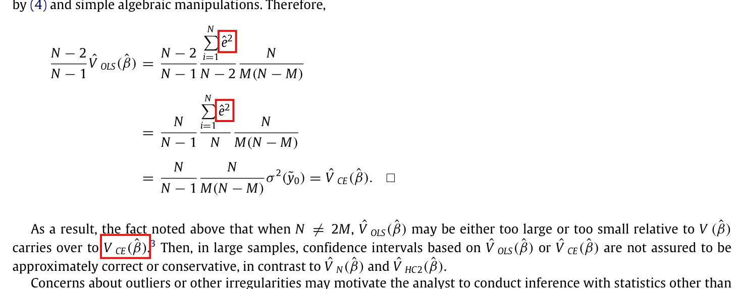
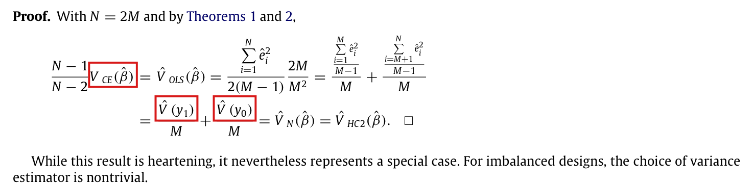
Standing assumptions: [Setting: Section 2, p. 366 (PDF p. 2)] Consider an experiment on a finite population $U$ of $N$ units in which $1 < M < N - 1$ units are randomly assigned to treatment and the remaining units are assigned to control. Denote control or treatment status, respectively, for unit $j$ with the random variable $X_j \in \{0, 1\}$ for which $\Pr(X_j = 1) = M/N$. Reassign an index ordering, $i = 1, \ldots, N$, such that those assigned to treatment come first, $X_1, \ldots, X_M = 1$ and those assigned to control come after, $X_{M+1}, \ldots, X_N = 0$. We observe $Y_i = X_i y_{1i} + (1 - X_i) y_{0i}$, (1) where $y_{1i}$ and $y_{0i}$ are unit $i$'s fixed “potential outcomes” under treatment and control, respectively. [Population moments: p. 366 (PDF p. 2)] Given a feature $v_i$ for $i \in 1, \ldots, N$, we define the population mean, $\bar v$, and variance, $\sigma^2(v)$, as, $\bar v = \frac{1}{N}\sum_{i=1}^{N} v_i$, $\sigma^2(v) = \frac{1}{N}\sum_{i=1}^{N}(v_i - \bar v)^2$. For features $v_i$ and $w_i$ for $i \in 1, \ldots, N$, we define the population covariance, $\sigma(v, w)$ as, $\sigma(v, w) = \frac{1}{N}\sum_{i=1}^{N}(v_i - \bar v)(w_i - \bar w)$. [Estimand: p. 366] We wish to estimate the average treatment effect, $\beta$, for the finite population $U$, $\beta = \overline{y_1} - \overline{y_0} = \frac{1}{N}\sum_{i=1}^{N}(y_{1i} - y_{0i})$. [Estimator and expectation: p. 366] $\hat\beta = \frac{1}{M}\sum_{i=1}^{M} Y_i - \frac{1}{N-M}\sum_{i=M+1}^{N} Y_i$, (2) with $E[\hat\beta] = \beta$, where the $E[\cdot]$ operator averages over all $\binom{N}{M}$ treatment assignments, each being equally likely. [Exact variance: p. 366; stated with a citation to Neyman (1923) and Freedman et al. (1998, A32–A34), not proved in the paper] $V(\hat\beta) = \frac{N}{N-1}\left[\frac{\sigma^2(y_1)}{M} + \frac{\sigma^2(y_0)}{N-M}\right] + \frac{1}{N-1}\left[2\sigma(y_1, y_0) - \sigma^2(y_1) - \sigma^2(y_0)\right]$. (3) [Regression form: p. 367 (PDF p. 3)] Define $Z = \begin{pmatrix} 1 & X_1 \\ \vdots & \vdots \\ 1 & X_N \end{pmatrix} = \begin{pmatrix} Z_1 \\ \vdots \\ Z_N \end{pmatrix}$, $Y = \begin{pmatrix} Y_1 \\ \vdots \\ Y_N \end{pmatrix}$. Then the regression estimator, $(Z'Z)^{-1}Z'Y = \begin{pmatrix} \hat\alpha \\ \hat\beta_{OLS} \end{pmatrix} = \begin{pmatrix} \frac{1}{N-M}\sum_{i=M+1}^{N} Y_i \\ \frac{1}{M}\sum_{i=1}^{M} Y_i - \frac{1}{N-M}\sum_{i=M+1}^{N} Y_i \end{pmatrix}$, (4) and so $\hat\beta_{OLS} = \hat\beta$ (Freedman, 2008b, Theorem 1). For future reference, define $\hat e_i = Y_i - Z_i(Z'Z)^{-1}Z'Y$, the regression residual. [Remarks for the formalizer, not printed in the paper] The re-indexing depends on the realized assignment: a sum over $i = 1, \ldots, M$ is a sum over the treated units $\{i : X_i = 1\}$ and a sum over $i = M+1, \ldots, N$ is a sum over the control units. The standing condition $1 < M < N - 1$ gives $M \ge 2$, $N - M \ge 2$ and $N \ge 4$, so the divisors $M - 1$, $N - M - 1$ and $N - 2$ are positive. Theorems 1 to 3 are identities in the observed data $(Y, X)$ that hold for every assignment; only Corollary 1 and the two large-sample statements involve the randomization distribution.

Effective claim (source TeX): Theorem 1. $\hat V_{HC2}(\hat\beta) = \hat V_N(\hat\beta)$. [No hypothesis is attached beyond the setting of Section 2.]

: T1Statement

Theorem: SAP.P031.T1

Statement hash: bdf8c71a29d919842eda9ecdcffae478298aa730086de4707ef1279c7999721e

Statement definition: SAP.P031.T1Statement

Certificate. 20261105T162217Z

Declaration review: faithful; 2026-11-05T17:36:05.249655Z; binding v2

Evidence scope: Certification checks formal proof objects. Statement fidelity is a model judgment. Author review is separate.

Proof dependencies: Independently extracted

Source and evidence metadata · sap-2026-11-08-assured-release

P031-T2

Corollary 1

p. 368 (PDF p. 4); supporting displays on p. 367 (PDF p. 3)

Corollary 1, p. 368 (PDF p. 4), displays p. 367 (PDF p. 3). Over uniform fixed-size assignments, expected HC2 is at least the actual randomization variance.

Historical component credits

Proved AronowAudit.P031.hc2_conservative Historical support retained; baseline fidelity: ok; manifest: used; used in Solution; This certifies expectation conservativeness, with no assertion of assignmentwise conservativeness or confidence-interval coverage.

Formal result: whole

Formal statement · Proof · Definitions

Assumptions and verification

Claim revision: catalog:06cd025683444fc7a32c7c84988353949147ed67bc1693055f68eba3b9bdb8fc

Effective claim (source TeX): Corollary 1. $E\left[\hat V_{HC2}(\hat\beta)\right] \ge V(\hat\beta)$. [No hypothesis is attached beyond the setting of Section 2.]

: T2Statement

Theorem: SAP.P031.T2

Statement hash: c4f8ecb738b7bc98ac5ece100ee0012be5f5036d37c5563bc07d9200f25ca94c

Statement definition: SAP.P031.T2Statement

Certificate. 20261105T162217Z

Declaration review: faithful; 2026-11-05T17:36:05.249655Z; binding v2

Evidence scope: Certification checks formal proof objects. Statement fidelity is a model judgment. Author review is separate.

Proof dependencies: Independently extracted

Source and evidence metadata · sap-2026-11-08-assured-release

P031-T3

Theorem 2

p. 369 (PDF p. 5)

Theorem 2, p. 369 (PDF p. 5). Multiplying OLS variance by (N-2)/(N-1) gives the constant-effects imputation variance.

Historical component credits

Proved AronowAudit.P031.scaled_ols_eq_constantEffects Historical support retained; baseline fidelity: ok; manifest: used; used in Solution; The imputation imposes a hypothesized effect equal to the estimate; actual effects need not be constant.

Formal result: whole

Formal statement · Proof · Definitions

Assumptions and verification

Claim revision: catalog:dbb2a34ac066c27b5e155a3a3cf25b5e21dd3706064b571d974e215a87c993d8

Effective claim (source TeX): Theorem 2. $\frac{N-2}{N-1}\hat V_{OLS}(\hat\beta) = \hat V_{CE}(\hat\beta)$. [No hypothesis is attached beyond the setting of Section 2.]

: T3Statement

Theorem: SAP.P031.T3

Statement hash: 57bddc4c9d8c7cdc15c3950d36b9847bb929b5fd12ef0b2048422e7fe8163a48

Statement definition: SAP.P031.T3Statement

Certificate. 20261105T162217Z

Declaration review: faithful; 2026-11-05T17:36:05.249655Z; binding v2

Evidence scope: Certification checks formal proof objects. Statement fidelity is a model judgment. Author review is separate.

Proof dependencies: Independently extracted

Source and evidence metadata · sap-2026-11-08-assured-release

P031-T4

Theorem 3

p. 369 (PDF p. 5); proof on p. 370 (PDF p. 6)

Theorem 3, p. 369 (PDF p. 5), proof p. 370 (PDF p. 6). In a balanced design the scaled constant-effects, OLS, Neyman, and HC2 estimators agree.

Historical component credits

Proved AronowAudit.P031.balanced_equivalences Historical support retained; baseline fidelity: ok; manifest: used; used in Solution; The CE scaling factor is part of the conclusion and must not be dropped when describing the four estimators as equal.

Formal result: whole

Formal statement · Proof · Definitions

Assumptions and verification

Claim revision: catalog:7d51e5759a712f173626b9380b0d4274148896b70a3be804ef8acf1d69f1a960

Effective claim (source TeX): Theorem 3. Under a balanced design such that $N = 2M$, $\frac{N-1}{N-2}\hat V_{CE}(\hat\beta) = \hat V_{OLS}(\hat\beta) = \hat V_N(\hat\beta) = \hat V_{HC2}(\hat\beta)$.

: T4Statement

Theorem: SAP.P031.T4

Statement hash: 8fe6feeb901fad8431391806dd8ee88e413611a5a342815d68eb60c1014c6500

Statement definition: SAP.P031.T4Statement

Certificate. 20261105T162217Z

Declaration review: faithful; 2026-11-05T17:36:05.249655Z; binding v2

Evidence scope: Certification checks formal proof objects. Statement fidelity is a model judgment. Author review is separate.

Proof dependencies: Independently extracted

Source and evidence metadata · sap-2026-11-08-assured-release

P031-T5

Unnumbered large-sample coverage statement (Section 3), its extension to HC2 after Corollary 1, and footnote 2

p. 367 (PDF p. 3); p. 368 (PDF p. 4), including footnote 2

pp. 367-368 (PDF pp. 3-4), including footnote 2. The cited regular finite-population regime gives the nonnegative finite Neyman bias, exact HC2 equality, asymptotic robust equivalences, and conservative normal-interval coverage. Restriction: the statement assumes strictly positive limiting N-times-true-variance contrast D; it does not formalize the D=0 coverage case. Allocation and moment conditions come from the cited regime, not from routine measure-theoretic defaults. A separate normality-only counterexample is retained as auxiliary evidence.

Historical component credits

Counterexample proved AronowAudit.P031.Wave1.printed_large_sample_contract_refuted Withdrawn support; baseline fidelity: ok; manifest: not listed; not used in Solution; Historical normality-only refutation does not address the repaired cited-regime effective claim. Preserve its original ok judgment as history; withdraw current claim credit. It is absent from the new manifest lists; no proof-dependency use is inferred.

Formal result: restricted

Scope: Strictly positive limiting N-times-true-variance contrast D>0; the D=0 coverage case is not formalized.

Formal statement · Proof · Definitions

Assumptions and verification

Claim revision: source-claim-import-2026-11-08:P031-T5:1

Effective claim (source TeX): [p. 367] The Neyman estimator is therefore conservative: its bias is always nonnegative. As demonstrated in Freedman (2008a, Theorem 1), asymptotic normality of $\hat\beta$ implies that large-sample confidence intervals, using $\hat V_N(\hat\beta)$ in a normal approximation will have either approximately correct or conservative coverage. [p. 368, after the proof of Corollary 1] Above, we noted that large-sample confidence intervals based on $\hat V_N(\hat\beta)$ had either approximately correct or conservative coverage. Clearly, this extends to $\hat V_{HC2}(\hat\beta)$. [p. 368, footnote 2] Implications for the other heteroskedasticity-robust estimators (HR, HC1, and HC3) studied in MacKinnon and White (1985) and Angrist and Pischke (2009, 299–308) are straightforward. The other estimators are all asymptotically equivalent to HC2 and, thus, large-sample confidence intervals based on any of the heteroskedasticity-robust estimators have either approximately correct or conservative coverage. [Contextual scope: The asymptotic assurances are read within the regular finite-population regime explicitly invoked through Freedman (2008a, Theorem 1), carried by the after-Corollary-1 reference, footnote 2 and Section 4 contrast. A corresponding two-arm formulation has N tending to infinity, M/N tending to p in (0,1), uniformly bounded fourth population moments, convergent first/second/mixed moments and positive limiting marginal variances. These are substantive conditions inferred from that invocation, not measure-theoretic defaults. Positive limiting contrast variance is not a condition of the coverage assurance: D=0 gives coverage tending to one.]

: SAP.P031.T5CitedRegimeStatement

Theorem: SAP.P031.T5

Statement hash: b27685952ae00e7b395a509775f7f828622128ea7007524fad8cf0f7cc70743c

Statement definition: SAP.P031.T5CitedRegimeStatement

Certificate. 20261105T162217Z

Declaration review: faithful; 2026-11-05T17:36:05.249655Z; binding v2

Evidence scope: Certification checks formal proof objects. Statement fidelity is a model judgment. Author review is separate.

Proof dependencies: Independently extracted

Source and evidence metadata · sap-2026-11-08-assured-release

P031-T6

Unnumbered statements on the homoskedastic OLS and constant-effects estimators when N is not 2M (Section 4)

p. 369 (PDF p. 5)

Section 4, p. 369 (PDF p. 5). Within the cited regular finite-population regime, unbalanced OLS and CE variance estimates can have either sign of asymptotic error and can yield undercoverage. Neyman and HC2 retain conservative normal-interval coverage. Restriction: the positive contrast assumes strictly positive limiting N-times-true-variance D and does not formalize the D=0 case. A separate normality-only counterexample is retained as auxiliary evidence. The once-unhatted CE quantity is the imputation estimator.

Historical component credits

Proved AronowAudit.P031.Wave1.ols_ce_may_be_too_small_or_large_proof Limited support; baseline fidelity: ok; manifest: not listed; not used in Solution; Historical positive variance-direction result is related partial evidence, without the repaired universal cited-regime Neyman/HC2 coverage contrast. It is absent from the new manifest lists; no actual proof-dependency use or nonuse is inferred.

Formal result: restricted

Scope: Strictly positive limiting N-times-true-variance contrast D>0; the D=0 coverage case is not formalized.

Formal statement · Proof · Definitions

Assumptions and verification

Claim revision: source-claim-import-2026-11-08:P031-T6:1

Effective claim (source TeX): [p. 369, before Theorem 2] Freedman (2008b, Theorem 5) demonstrates that for $N \neq 2M$, $\hat V_{OLS}(\hat\beta)$ converges asymptotically to a limit that may be too big or too small relative to $V(\hat\beta)$. [p. 369, after the proof of Theorem 2] As a result, the fact noted above that when $N \neq 2M$, $\hat V_{OLS}(\hat\beta)$ may be either too large or too small relative to $V(\hat\beta)$ carries over to $V_{CE}(\hat\beta)$. Then, in large samples, confidence intervals based on $\hat V_{OLS}(\hat\beta)$ or $\hat V_{CE}(\hat\beta)$ are not assured to be approximately correct or conservative, in contrast to $\hat V_N(\hat\beta)$ and $\hat V_{HC2}(\hat\beta)$. [As printed, $V_{CE}(\hat\beta)$ in the second passage has no hat. Footnote 3, attached to that sentence, is not part of the target. No asymptotic sequence or condition is restated here. Contextual scope: The asymptotic assurances are read within the regular finite-population regime explicitly invoked through Freedman (2008a, Theorem 1), carried by the after-Corollary-1 reference, footnote 2 and Section 4 contrast. A corresponding two-arm formulation has N tending to infinity, M/N tending to p in (0,1), uniformly bounded fourth population moments, convergent first/second/mixed moments and positive limiting marginal variances. These are substantive conditions inferred from that invocation, not measure-theoretic defaults. Positive limiting contrast variance is not a condition of the coverage assurance: D=0 gives coverage tending to one.]

: SAP.P031.T6CitedRegimeStatement

Theorem: SAP.P031.T6

Statement hash: c36ca44bcf6102db0a2b4d7e3cba95f08df11a2a3b452787bf0a07f51e6e33fa

Statement definition: SAP.P031.T6CitedRegimeStatement

Certificate. 20261105T162217Z

Declaration review: faithful; 2026-11-05T17:36:05.249655Z; binding v2

Evidence scope: Certification checks formal proof objects. Statement fidelity is a model judgment. Author review is separate.

Proof dependencies: Independently extracted

Source and evidence metadata · sap-2026-11-08-assured-release

P031-T7

Proof of Theorem 2, first sentence, as printed

p. 369 (PDF p. 5)

first sentence of the proof of Theorem 2, p. 369 (PDF p. 5). The specified four-unit assignment has both imputed variances 5/2 and original potential-outcome covariance 23/2, refuting the printed covariance equality.

Historical component credits

Counterexample proved AronowAudit.P031.printed_covariance_counterexample Historical support retained; baseline fidelity: ok; manifest: used; used in Solution; This is an exact witness against the untilded proof equality, and does not refute Theorem 2.

Formal result: whole

Formal statement · Proof · Definitions

Assumptions and verification

Claim revision: catalog:93b8391d1f0f059f427f493bdf84d6dc5c86234f341ca826f11369120d849d2a

Effective claim (source TeX): [Printed statement: p. 369 (PDF p. 5), first sentence of the proof of Theorem 2 and the display it introduces] Proof. Since $\tilde y_0 = \tilde y_1 - \hat\beta$, $\sigma^2(\tilde y_0) = \sigma^2(\tilde y_1) = \sigma(y_0, y_1)$. Thus, substituting this into expression (5), randomization yields, $\hat V_{CE}(\hat\beta) = \frac{N}{N-1}\frac{N}{M(N-M)}\sigma^2(\tilde y_0)$. [Counterexample to the last equality of the printed sentence, $\sigma^2(\tilde y_1) = \sigma(y_0, y_1)$; from the validator] Let $N = 4$ and $M = 2$, so that $1 < M < N - 1$. Let the potential outcomes be $y_0 = y_1 = (0, 2, 5, 9)$ and let units 1 and 2 be treated, $X = (1, 1, 0, 0)$, which is one of the $\binom{4}{2} = 6$ equally likely assignments. Then $Y = (0, 2, 5, 9)$, $\frac{1}{M}\sum_{i=1}^{M} Y_i = 1$, $\frac{1}{N-M}\sum_{i=M+1}^{N} Y_i = 7$, $\hat\alpha = 7$, $\hat\beta = -6$, $\tilde y_0 = (6, 8, 5, 9)$ and $\tilde y_1 = (0, 2, -1, 3)$, so that $\tilde y_0 = \tilde y_1 - \hat\beta$ holds. The values are $\sigma^2(\tilde y_0) = \sigma^2(\tilde y_1) = \frac{5}{2}$ and $\sigma(y_0, y_1) = \frac{23}{2}$. Hence $\sigma^2(\tilde y_0) = \sigma^2(\tilde y_1) \neq \sigma(y_0, y_1)$ in an instance that satisfies every condition of Section 2.

: T7Statement

Theorem: SAP.P031.T7

Statement hash: 4ae7256cb359a28e092f2c2b23d8da60caeb38cdbb2a9439a54f0dafe837c1f8

Statement definition: SAP.P031.T7Statement

Certificate. 20261105T162217Z

Declaration review: faithful; 2026-11-05T17:36:05.249655Z; binding v2

Evidence scope: Certification checks formal proof objects. Statement fidelity is a model judgment. Author review is separate.

Proof dependencies: Independently extracted

Source and evidence metadata · sap-2026-11-08-assured-release

P031-T8

Proof of Theorem 2, corrected

p. 369 (PDF p. 5)

corrected proof of Theorem 2, p. 369 (PDF p. 5). Every link of the corrected imputed-moment, residual-sum, and scaled-OLS proof chain holds.

Historical component credits

Proved AronowAudit.P031.corrected_theorem_two_proof Historical support retained; baseline fidelity: ok; manifest: used; used in Solution; The corrected target, rather than the false untilded printed proof step, is the assigned component.

Formal result: whole

Formal statement · Proof · Definitions

Assumptions and verification

Claim revision: catalog:957da3e23ba7e4d65d076bf73ef9b06ff65e6c6c6295f9a7bfa6fbf938075df2

Effective claim (source TeX): [Corrected proof of Theorem 2, p. 369 (PDF p. 5). Two corrections: $\sigma(\tilde y_0, \tilde y_1)$ replaces the printed $\sigma(y_0, y_1)$ in the first sentence, and $\hat e_i^2$ replaces the printed $\hat e^2$ in the two residual sums of the last display. Everything else is as printed.] [Hypotheses] The setting of Section 2: a finite population of $N$ units of which $M$ are treated, with $1 < M < N - 1$. The identities hold for every assignment of exactly $M$ units to treatment and for all real values of the observed outcomes $Y_1, \ldots, Y_N$; nothing is assumed about the potential outcomes $y_{0i}$, $y_{1i}$, and in particular constant effects are not assumed. [Statement] Since $\tilde y_0 = \tilde y_1 - \hat\beta$, $\sigma^2(\tilde y_0) = \sigma^2(\tilde y_1) = \sigma(\tilde y_0, \tilde y_1)$. Thus, substituting this into expression (5), randomization yields, $\hat V_{CE}(\hat\beta) = \frac{N}{N-1}\frac{N}{M(N-M)}\sigma^2(\tilde y_0)$. Now, taking $\hat\alpha$ and $\hat\beta$ as fixed, $\frac{\sum_{i=1}^{N}\hat e_i^2}{N} = \frac{\sum_{i=1}^{N}\left(Y_i - \hat\alpha - X_i\hat\beta\right)^2}{N} = \frac{\sum_{i=1}^{N}\left(\tilde y_{0i} - \hat\alpha\right)^2}{N} = \sigma^2(\tilde y_0)$, by (4) and simple algebraic manipulations. Therefore, $\frac{N-2}{N-1}\hat V_{OLS}(\hat\beta) = \frac{N-2}{N-1}\frac{\sum_{i=1}^{N}\hat e_i^2}{N-2}\frac{N}{M(N-M)} = \frac{N}{N-1}\frac{\sum_{i=1}^{N}\hat e_i^2}{N}\frac{N}{M(N-M)} = \frac{N}{N-1}\frac{N}{M(N-M)}\sigma^2(\tilde y_0) = \hat V_{CE}(\hat\beta)$. [The corrected proof thus asserts four identities, each for every assignment] (i) $\sigma^2(\tilde y_0) = \sigma^2(\tilde y_1) = \sigma(\tilde y_0, \tilde y_1)$; (ii) $\hat V_{CE}(\hat\beta) = \frac{N}{N-1}\frac{N}{M(N-M)}\sigma^2(\tilde y_0)$, from (i) and expression (5); (iii) $\frac{1}{N}\sum_{i=1}^{N}\hat e_i^2 = \sigma^2(\tilde y_0)$; (iv) the last displayed chain, whose two ends are Theorem 2.

: T8Statement

Theorem: SAP.P031.T8

Statement hash: 0f96d204899d4dac7c9bd554b80450c784d01b204f3bfa7d7e91ac66bab76107

Statement definition: SAP.P031.T8Statement

Certificate. 20261105T162217Z

Declaration review: faithful; 2026-11-05T17:36:05.249655Z; binding v2

Evidence scope: Certification checks formal proof objects. Statement fidelity is a model judgment. Author review is separate.

Proof dependencies: Independently extracted

Source and evidence metadata · sap-2026-11-08-assured-release

P031-T9

Proof of Theorem 3, corrected

p. 370 (PDF p. 6)

corrected proof of Theorem 3, p. 370 (PDF p. 6). Every link of the balanced-design chain holds, with the CE hat and sample-variance notation restored.

Historical component credits

Proved AronowAudit.P031.corrected_theorem_three_proof Historical support retained; baseline fidelity: ok; manifest: used; used in Solution; The corrected target restores the CE hat and the sample-variance notation without changing the mathematical identity.

Formal result: whole

Formal statement · Proof · Definitions

Assumptions and verification

Claim revision: catalog:a39dadb1c9720257e73c249700588c193411fbbc29878d638987e470f27e4092

Effective claim (source TeX): [Corrected proof of Theorem 3, p. 370 (PDF p. 6). Two corrections: $\hat V_{CE}(\hat\beta)$ replaces the printed $V_{CE}(\hat\beta)$ in the first term, and $\hat\sigma^2(y_1)$, $\hat\sigma^2(y_0)$ replace the printed $\hat V(y_1)$, $\hat V(y_0)$. Everything else is as printed.] [Hypotheses] The setting of Section 2 under a balanced design such that $N = 2M$; the standing condition $1 < M < N - 1$ then gives $M \ge 2$ and $N - M = M$. The identities hold for every assignment of exactly $M$ units to treatment and for all real values of the observed outcomes $Y_1, \ldots, Y_N$. [Statement] With $N = 2M$ and by Theorems 1 and 2, $\frac{N-1}{N-2}\hat V_{CE}(\hat\beta) = \hat V_{OLS}(\hat\beta) = \frac{\sum_{i=1}^{N}\hat e_i^2}{2(M-1)}\frac{2M}{M^2} = \frac{\frac{\sum_{i=1}^{M}\hat e_i^2}{M-1}}{M} + \frac{\frac{\sum_{i=M+1}^{N}\hat e_i^2}{M-1}}{M} = \frac{\hat\sigma^2(y_1)}{M} + \frac{\hat\sigma^2(y_0)}{M} = \hat V_N(\hat\beta) = \hat V_{HC2}(\hat\beta)$.

: T9Statement

Theorem: SAP.P031.T9

Statement hash: 609cbb247fe9c4ded9b7409dca8e5310addef33598dd41392830527ff6c508ec

Statement definition: SAP.P031.T9Statement

Certificate. 20261105T162217Z

Declaration review: faithful; 2026-11-05T17:36:05.249655Z; binding v2

Evidence scope: Certification checks formal proof objects. Statement fidelity is a model judgment. Author review is separate.

Proof dependencies: Independently extracted

Source and evidence metadata · sap-2026-11-08-assured-release

P031-T10

Footnote 3, as printed

p. 369 (PDF p. 5), footnote 3

counterexample to footnote 3, p. 369 (PDF p. 5), parts (a)–(c). Shifting all control outcomes by c and all treatment outcomes by c+d shifts the control mean and population effect by c and d. Assignment by assignment, it adds c+dX to the observed vector, shifts the intercept and treatment estimate by c and d, and preserves every residual, OLS variance estimate, and actual randomization variance. For N=4k, M=k, k≥2, the balanced sign schedules y0=z, y1=a z+2, a=1,2,1/2, share allocation 1/4, control mean 0 and effect 2. Their moments and exact N-times-variance and OLS formulas hold, with the treated sign mean r satisfying E[r²]=3/(N-1). Their true leading limits are 16/3,49/3,25/12, their OLS probability and expectation limits are 16/3,28/3,13/3, and their OLS/actual-variance probability-limit ratios are 1,4/7,52/25. At k=2 the printed outcome vectors give 28 assignments, actual variances 16/21,7/3,25/84, expected OLS estimates 16/21,8/7,2/3 and expectation/variance ratios 1,24/49,56/25. Thus allocation and the two first moments do not determine the variance relation. The usual measure-theoretic conditions are assumed.

Historical component credits

Counterexample proved AronowAudit.P031.footnote_three_counterexample Historical support retained; baseline fidelity: ok; manifest: used; used in Solution; {'source': 'adjudication', 'decision': 'rejected', 'what': 'At AronowAudit/P031/P031_Variance.lean:2376, the conjunction supplies all three specified families, their common allocation and first moments, the distinct probability limits 1, 4/7 and 52/25, and universal invariance of both variances under the specified shifts; FootnoteVarianceWitness is expanded at line 2278. This matches the asymptotic counterexample and variance-invariance component identified by the row, without restricting its populations or assignments. The exact finite formulas, N=8 enumeration and intercept/residual identities are separate supporting components of the expanded target, so their absence from this declaration does not omit a conclusion of the credited component. The additional CE probability limit strengthens the witness harmlessly.'}

Formal result: whole

Formal statement · Proof · Definitions

Assumptions and verification

Claim revision: catalog:09cecd529551b564b9284d0ca8112a577ec7cb579a217cff95b7403ff51bfa56

Effective claim (source TeX): [Printed statement: p. 369 (PDF p. 5), footnote 3] Freedman (2008b, p. 190) gives the exact asymptotic relation between $\hat V_{OLS}(\hat\beta)$ and $V(\hat\beta)$, which depends on the size of the treatment versus control group and the limiting values of the control group mean and average treatment effect. [Counterexample from the validator, to the claim that the relation depends on the limiting values of the control group mean $\overline{y_0}$ and the average treatment effect $\beta$. Part (a) shows that these two quantities can take any values without changing either variance; part (b) shows that fixing them, together with the allocation, does not fix the relation.] (a) Exact invariance, for every finite population in the setting of Section 2 and every assignment. For real constants $c$ and $d$ let $y'_{0i} = y_{0i} + c$ and $y'_{1i} = y_{1i} + c + d$ for all $i$. Then $\overline{y'_0} = \overline{y_0} + c$ and $\beta' = \beta + d$. For each assignment the observed outcomes become $Y'_i = Y_i + c + dX_i$, so $\hat\alpha' = \hat\alpha + c$, $\hat\beta' = \hat\beta + d$, every residual $\hat e_i$ is unchanged and $\hat V_{OLS}(\hat\beta') = \hat V_{OLS}(\hat\beta)$; and $V(\hat\beta') = V(\hat\beta)$. (b) Three sequences of populations. For each integer $k \ge 2$ let $N = 4k$ and $M = k$, let $z_i = -1$ for $i = 1, \ldots, 2k$ and $z_i = +1$ for $i = 2k+1, \ldots, 4k$, and let $y_{0i} = z_i$ and $y_{1i} = a z_i + 2$, for each of $a = 1$, $a = 2$ and $a = 1/2$. For every $k$ and each $a$: $M/N = 1/4$, $\overline{y_0} = 0$, $\overline{y_1} = 2$, $\beta = 2$, $\sigma^2(y_0) = 1$, $\sigma^2(y_1) = a^2$ and $\sigma(y_1, y_0) = a$. Exactly, $N V(\hat\beta) = \frac{N}{N-1}\left(3a^2 + 2a + \frac{1}{3}\right)$, and for each assignment $N\hat V_{OLS}(\hat\beta) = \frac{N}{N-2}\left[\frac{4a^2}{3} + 4 - \left(\frac{4a^2}{3} + \frac{4}{9}\right)r^2\right]$, where $r$ is the mean of $z_i$ over the treated units and $E[r^2] = \frac{3}{N-1}$. Hence, as $k \to \infty$, $N V(\hat\beta) \to 3a^2 + 2a + \frac{1}{3}$ and $N\hat V_{OLS}(\hat\beta) \to \frac{4a^2}{3} + 4$ in probability, and $N E\left[\hat V_{OLS}(\hat\beta)\right]$ has the same limit. The limiting ratio of $\hat V_{OLS}(\hat\beta)$ to $V(\hat\beta)$ is $1$ for $a = 1$ ($\frac{16}{3}$ against $\frac{16}{3}$), $\frac{4}{7}$ for $a = 2$ ($\frac{28}{3}$ against $\frac{49}{3}$) and $\frac{52}{25}$ for $a = 1/2$ ($\frac{13}{3}$ against $\frac{25}{12}$), with the same allocation, the same control group mean and the same average treatment effect in all three. (c) Exact finite instance of (b) at $k = 2$: $N = 8$, $M = 2$, $y_0 = (-1, -1, -1, -1, 1, 1, 1, 1)$, and $y_1$ equal to $(1, 1, 1, 1, 3, 3, 3, 3)$, $(0, 0, 0, 0, 4, 4, 4, 4)$ or $\left(\frac{3}{2}, \frac{3}{2}, \frac{3}{2}, \frac{3}{2}, \frac{5}{2}, \frac{5}{2}, \frac{5}{2}, \frac{5}{2}\right)$. Over all $\binom{8}{2} = 28$ assignments, $V(\hat\beta) = \frac{16}{21}$, $\frac{7}{3}$, $\frac{25}{84}$ and $E\left[\hat V_{OLS}(\hat\beta)\right] = \frac{16}{21}$, $\frac{8}{7}$, $\frac{2}{3}$ respectively, so the ratio $E\left[\hat V_{OLS}(\hat\beta)\right]/V(\hat\beta)$ is $1$, $\frac{24}{49}$, $\frac{56}{25}$, at the same $M/N = 1/4$, $\overline{y_0} = 0$ and $\beta = 2$.

: SAP.P031.T10WholeStatement

Theorem: SAP.P031.T10

Statement hash: 3f8734d59f45047df82bbf3d25e558944209d06bbd9aa219c9551a0d5cd5aa96

Statement definition: SAP.P031.T10WholeStatement

Certificate. 20261105T162217Z

Declaration review: faithful; 2026-11-05T17:36:05.249655Z; binding v2

Evidence scope: Certification checks formal proof objects. Statement fidelity is a model judgment. Author review is separate.

Proof dependencies: Independently extracted

Source and evidence metadata · sap-2026-11-08-assured-release

P031-T11

Footnote 3, corrected

p. 369 (PDF p. 5), footnote 3

corrected footnote 3, p. 369 (PDF p. 5). Interior allocation and convergent population second moments give the corrected variance, expected-OLS, bias, treatment-effect-variance, conditional probability, and positive-denominator ratio limits, with bounded-outcome sufficiency and exact shifts. Sample second-moment convergence means consistency of both centered arm sample variances.

Historical component credits

Proved AronowAudit.P031.Wave1.footnote_three_complete Historical support retained; baseline fidelity: ok; manifest: used; used in Solution; {'source': 'adjudication', 'decision': 'rejected', 'what': 'At AronowAudit/P031/Wave1/FootnoteThreeComplete.lean:10, the hypotheses and deterministic limits match the corrected claim, including the difference and treatment-effect-variance limits, and the conclusion includes the optional probability/ratio limits and exact variance shift invariance. ArmSecondMomentsConverge, defined in P031/P031_Variance.lean:2417, expresses consistency of the centered arm sample variances, the second moments used by the OLS formula. This loses no case under the usual finite raw-second-moment reading either: interior allocation and convergent population variances give sample-mean consistency, and convergent finite raw second moments then give centered sample-variance consistency. Uniform boundedness and positive leading variance are used only where the corrected claim places them, so the note does not identify a material restriction.'}
Proved AronowAudit.P031.Wave1.footnote_three_probability_complete Historical support retained; baseline fidelity: ok; manifest: used; used in Solution; {'source': 'adjudication', 'decision': 'rejected', 'what': 'At AronowAudit/P031/Wave1/FootnoteThreeProbability.lean:18, the theorem proves precisely the stochastic component: uniformly bounded outcomes imply arm-variance consistency, that consistency gives the scaled OLS probability limit, and positive leading true variance gives the ratio limit. These are conclusions and conditions expressly present in the corrected claim, rather than extra assumptions imported from the row description. The centered second-moment formulation in P031/P031_Variance.lean:2417 preserves the ordinary finite raw-second-moment cases as well, because sample means are consistent under the stated allocation and population-variance limits. The deterministic and shift clauses belong to the separately credited complete declaration and need not be repeated in this stochastic component.'}

Formal result: restricted

Scope: States every mathematical clause of the corrected footnote; excludes the bibliographic assertion that Freedman (2008b, p. 190) gives the relation.

Formal statement · Proof · Definitions

Assumptions and verification

Claim revision: catalog:9b757199f55b3bb9ab4ac3b294c49752a04d15fb339e2007c45b22279b70ff1a

Effective claim (source TeX): [Corrected footnote 3, p. 369 (PDF p. 5). One correction: “the limiting variances and covariance of the treatment and control potential outcomes” replaces the printed “the limiting values of the control group mean and average treatment effect”.] Freedman (2008b, p. 190) gives the exact asymptotic relation between $\hat V_{OLS}(\hat\beta)$ and $V(\hat\beta)$, which depends on the size of the treatment versus control group and the limiting variances and covariance of the treatment and control potential outcomes. [The relation in full, with every hypothesis, from the validator's derivation. These conditions are the validator's and are not printed in the paper.] Consider a sequence of finite populations, each in the setting of Section 2 ($N$ units, $M$ of them treated, $1 < M < N - 1$, all $\binom{N}{M}$ assignments equally likely), with $N \to \infty$, $M/N \to p \in (0, 1)$, $\sigma^2(y_1) \to v_1$, $\sigma^2(y_0) \to v_0$ and $\sigma(y_1, y_0) \to c$. Then $\lim N V(\hat\beta) = \frac{1-p}{p}v_1 + \frac{p}{1-p}v_0 + 2c$ and $\lim N E\left[\hat V_{OLS}(\hat\beta)\right] = \frac{v_1}{1-p} + \frac{v_0}{p}$, so that $\lim N\left(E\left[\hat V_{OLS}(\hat\beta)\right] - V(\hat\beta)\right) = \frac{(2p-1)(v_1 - v_0)}{p(1-p)} + v_1 + v_0 - 2c$, where $v_1 + v_0 - 2c$ is the limit of $\sigma^2(y_1 - y_0)$, the variance of the unit-level treatment effects. If in addition the sample second moments converge, for which it suffices that the potential outcomes are uniformly bounded along the sequence, then $N\hat V_{OLS}(\hat\beta) \to \frac{v_1}{1-p} + \frac{v_0}{p}$ in probability, and when $\frac{1-p}{p}v_1 + \frac{p}{1-p}v_0 + 2c > 0$ the ratio $\hat V_{OLS}(\hat\beta)/V(\hat\beta)$ converges in probability to $\left(\frac{v_1}{1-p} + \frac{v_0}{p}\right)\Big/\left(\frac{1-p}{p}v_1 + \frac{p}{1-p}v_0 + 2c\right)$. The limits depend on the sequence only through $p$, $v_1$, $v_0$ and $c$. No first moment enters: for real constants $c'$ and $d$, replacing every $y_{0i}$ by $y_{0i} + c'$ and every $y_{1i}$ by $y_{1i} + c' + d$ changes $\overline{y_0}$ to $\overline{y_0} + c'$ and $\beta$ to $\beta + d$ and leaves $V(\hat\beta)$ and, for every assignment, $\hat V_{OLS}(\hat\beta)$ unchanged.

: T11Statement

Theorem: SAP.P031.T11

Statement hash: bbe4c03e85e89c305863ad4910035dce569a387aca030393ffef9c942edb43d8

Statement definition: SAP.P031.T11Statement

Certificate. 20261105T162217Z

Declaration review: faithful; 2026-11-05T17:36:05.249655Z; binding v2

Evidence scope: Certification checks formal proof objects. Statement fidelity is a model judgment. Author review is separate.

Proof dependencies: Independently extracted

Source and evidence metadata · sap-2026-11-08-assured-release

Reproduction

What I recalculated or reran from public materials. "Agrees", "Agrees in part" or "Disagrees" compares my result with the printed one. "Not compared" means the comparison could not be made.

Status: Not applicable
Agreement: Not applicable