Journal article P039

Corrections to: Ideologically Extreme Candidates in U.S. Presidential Elections, 1948-2012

Marty Cohen, Mary C. McGrath, P. M. Aronow, and John Zaller (2016). Ideologically Extreme Candidates in U.S. Presidential Elections, 1948-2012. Annals of the American Academy of Political and Social Science 667(1):126–142.

DOI: 10.1177/0002716216660571
Audited edition: Annals of the American Academy of Political and Social Science, 2016, 667(1):126–142; 17 pages in the audited file
SHA-256 of the audited file: 691cbd132a33b4ba7cf2cb30d7a2a77829efb8dea0183f833d85d7534aef6ec3
Permanent address: https://pmaronow.github.io/llm-audit/works/P039/

Summary

The paper asks whether ideologically extreme candidates are penalized in U.S. presidential elections. It adds five measures of the incumbent-party candidate’s relative extremism to two models of the vote, “musical chairs” and “bread and peace”, fitted to the elections of 1948–2012. It finds scant evidence of a penalty that is large or close to statistical significance. 9 entries are classified as errors (9 Minor), and 4 are clarity notes. None changes a conclusion. Four further questions could not be settled from the available sources.

What was and was not checked

I checked the results below by recalculating them from the replication files, which contain the scripts and the derived data (the ideology scores and the data for Figures 3 and 4).

Table 1. All 15 correlations and all case counts reproduce. The two correlations on the eight elections with NOMINATE scores are the subject of P039-N006.
Table 2. In Panel A, the coefficients and standard errors for incumbent fatigue, war fatalities and relative extremism reproduce in all three columns, as do the constants, the numbers of cases, the adjusted $R^2$ and the root mean squared errors. The income row differs (P039-E003). In Panel B, every coefficient, standard error, decay parameter, constant and number of cases reproduces by nonlinear least squares with the archived formula, which uses quarters 2–16 (P039-E001). Three fit statistics differ in the last digit (P039-N008). The significance stars in both panels agree with the recomputed p-values.
Table 3. All ten maximum effects, p-values and degrees of freedom reproduce, and eight of the ten coefficients are negative, as the text says. The worked example on p. 139 reproduces, with the value $+1.38$ . Two location scores quoted with it and the election named in note 15 are the subjects of P039-N010 and P039-E004.
Figures. The correlations $.97$ and $.75$ of Figure 2 reproduce. The points of Figures 3 and 4 agree with the data and with the recomputed residuals. This agreement was judged by eye, since the paper prints no slopes. The p-value of $.26$ quoted for Figure 4B reproduces as a number, and its use is the subject of P039-E002.
Data. The spliced location scores regenerate from the archived scripts to within floating-point precision, and so do the four scores of relative extremism that are based on the ANES and Rosenstone ratings. The vote shares, the vote margins, the incumbent-party indicator and the tenure variable are correct for all seventeen elections.
Text. The statements on p. 131 about Figure 1 agree with the scores, apart from the one in P039-N005. The pooled within-party variance of the refined locations is $1.55$ times that of the all-voter locations, in line with “about 50 percent more year-to-year variation” on p. 130. The check described in note 14 gives weak effects in both models. The historical examples in the conclusion agree with the scores, the tenure variable, income growth and the outcomes.
The main conclusion. The smallest p-value in the ten tests is $.30$ . With quarter 1 restored to the income measure of the bread and peace models, the five extremism coefficients remain negative and far from significance. The estimates are imprecise. The 95 percent interval for the largest effect in the featured bread and peace model runs from about $-1.4$ to $+4.2$ points of vote share. The featured coefficient moves from $-2.23$ ( $p=.30$ ) to $-4.35$ ( $p=.10$ ) when the election of 1980 is left out. The paper says that weak evidence of an effect is not evidence that none exists.

The following were not checked.

The online appendix cited in note 7 was not available. The model that removes partisan bias from the ANES placements was read from the code, and it could not be compared with its description in the appendix.
The replication files do not contain the ANES cumulative file, the NOMINATE file, the quarterly income and price series or Hibbs’s data file. The scripts that construct the location scores from the survey responses, the NOMINATE scores and the income and war variables were read and could not be run. Four questions remain undetermined for lack of these sources or of a stated rule. Two concern how the high-information respondents are selected, one the comparison of income series in note 4, and one the choice between Johnson’s two NOMINATE scores for 1964.
I did not consult the cited works themselves. I did not check the paper’s descriptions of them, the quotation from Hibbs or the page references in note 16. I compared three entries in the reference list with public catalogue and publisher information (P039-E008, P039-N013).

These checks cover what can be recomputed from the derived data. They do not show that the paper is free of other errors.

Headline claims and related corrections

In ten tests (five measures of the incumbent-party candidate's relative extremism, each in two baseline vote models) on the postwar presidential elections, there is scant evidence of an extremism penalty that is substantively large or close to statistical significance; relative ideological location is not an important predictor of presidential election outcomes.
Abstract (p. 126); introduction (p. 127); pp. 139–140; Table 3 (all ten models); Table 2 columns A3 and B3; Figure 4
See P039-E001, P039-E002, P039-E004.
All five relative-extremism measures correlate negatively but weakly with incumbent-party vote share. The larger NOMINATE correlation, $-0.48$ , reflects the eight elections with available scores: the paper reports correlations of $-0.44$ for both zero-centered perception measures on those cases.
p. 134 (PDF p. 9); Table 1 (p. 135)
See P039-N006.
Controlling for the three fundamentals, a one-point increase in refined, zero-centered relative extremism is associated with a $0.46$ -point lower incumbent vote margin in the musical-chairs model and a $2.23$ -point lower two-party share in the bread-and-peace model. Neither estimate is near statistical significance; Figure 4 is described as showing a null relationship in panel A and a weak one in panel B, with $p=0.26$ .
p. 138 (PDF p. 13); Table 2 columns A3 and B3; Figure 4
See P039-E002, P039-E001.
The largest predicted effect in the ten models is described as modest, including a $1.38$ -point vote-share gain for Carter in 1980 under the featured bread-and-peace specification. The extremism coefficient has the expected negative sign in eight of the ten models.
p. 139 (PDF p. 14); Table 3; note 15
See P039-E004, P039-N010.
The paper reports correlations of $+0.97$ between the ANES/Rosenstone and NOMINATE location scores and $+0.75$ between their absolute values. It suggests that the latter correlation is high enough to make both measures worth taking seriously, while acknowledging uncertainty about how reassuring it is. Both candidates have NOMINATE scores in eight of the seventeen elections.
p. 131 (PDF p. 6); Figure 2
The musical-chairs and bread-and-peace models replicate on updated data, and the three fundamentals (income growth, incumbent-party tenure, war fatalities) account for much of the variation in presidential outcomes; income growth is strongly related to vote share while relative candidate extremism adds little explanatory force.
pp. 127, 135–136 and 140; Table 1; Table 2 (columns A1, A2, B1, B2); Figures 3–4
See P039-E003, P039-E001, P039-E002, P039-N008.
Goldwater and McGovern lost under unfavourable fundamentals (incumbent parties in their first term, strong economies), whereas Reagan in 1980 and Obama in 2008 were rated almost as extreme and won against incumbent parties with poor economic records; and moderation does not guarantee victory, since the rated moderates Dewey (1948), Nixon (1960) and Carter (1980) all lost.
Conclusion, p. 140 (PDF p. 15); Figure 1; the data behind Table 2 and Figure 3
There is little evidence of an electorally important relationship between candidate extremism and vote outcomes, though this is not evidence that none exists, nor that voters ignore candidates' policy positions; Converse's view that voters respond to the nature of the times and not to ideology stands up better to postwar presidential elections than Downs's median voter theorem.
Conclusion, pp. 140–141 (PDF pp. 15–16); Tables 2 and 3 as a whole

Sources that could not be obtained

Online appendix with details of the model, cited in note 7 (printed p. 141, PDF p. 16) at http://ann.sagepub.com/supplemental

Corrections

Minor (9)

Real but inconsequential, for example a misprint that does not change a result.

P039-E001 Minor

The income measure in every bread and peace model that was fitted covers quarters 2–16 of the presidential term, and not quarters 1–16 as the text and Table 2 say.

Paragraph on Panel B of Table 2, p. 136 (PDF p. 11); section “The `bread and peace' model”, p. 128 (PDF p. 3); Table 2, Bread & Peace panel, first row label, p. 137 (PDF p. 12)

See also under Formal statements (Lean): P039-T1, P039-T2

As printed

p. 128: “While Hibbs, like Achen and Bartels (2016), also employs change in RDI to measure economic performance, bread and peace allows RDI growth from every quarter of a presidential term to factor into the model, albeit discounted over time so that earlier quarters carry less weight. Hibbs applies a decay parameter— $\lambda$ , estimated within the model as a number between 0 and 1—to progressively discount economic growth in earlier quarters of the presidential term. This discounting takes the following form: Because the election is held one-third of the way through the 16th quarter of a presidential term, RDI growth in this quarter is down-weighted by $\tfrac{1}{3} * \lambda^{0}$ . The 15th quarter of the presidential term is down-weighted by $\lambda^{1}$ , the 14th quarter by $\lambda^{2}$ , and so on for the preceding quarters.”

p. 136: “The dependent variable in Panel B is incumbent party share of the two-party vote, and RDI is measured using Hibbs’s definition of the variable, with quarters 1–16 discounted by a decay parameter as described above.”

Table 2, p. 137, Bread & Peace panel, first row label: “ $\Delta$ weighted RDI in Q 1-16”

The problem

The paragraph on p. 136 says that the income measure in Panel B of Table 2 discounts quarters 1–16, and the row label in the table repeats this range. The description on p. 128 assigns the weight $1/3$ to quarter 16, the weight $\lambda$ to quarter 15 and the weight $\lambda^{2}$ to quarter 14, “and so on for the preceding quarters”. Carried back to the start of the term, this rule implies that quarter 1 has the weight $\lambda^{15}$ . The models that were fitted stop at quarter 2. Let $h_q$ be the annualized growth of real disposable income in quarter $q$ of the term. The replication files contain nine formulas that are fitted by nonlinear least squares, eight for Tables 2 and 3 and one for Figure 4B. In each of them the income measure is

G_{15}=\frac{h_{16}/3+\sum_{k=1}^{14}\lambda^{k}h_{16-k}}{1/3+\sum_{k=1}^{14}\lambda^{k}}.

The growth $h_1$ of the first quarter is in the data for each of the sixteen elections of 1952–2012, and it enters none of the formulas. The stated range is therefore not the range of the fitted models. Hibbs (2012) and the online appendix were not available. I could not determine whether Hibbs’s own specification uses fifteen or sixteen quarters, or whether quarter 1 was left out on purpose.

Evidence an exact counterexample

The evidence is a check of the nine formulas, an exact counterexample which shows that the two measures differ, and a refit of the models. I write $N_{15}$ and $D_{15}$ for the numerator and the denominator of $G_{15}$ . The measure as described, with quarter 1 included, is

G_{16}=\frac{N_{15}+\lambda^{15}h_1}{D_{15}+\lambda^{15}}.

Subtracting $G_{15}$ , I obtain

G_{16}-G_{15}=\frac{\lambda^{15}}{D_{15}+\lambda^{15}}\,(h_1-G_{15}).

For $0<\lambda<1$ , the two measures agree only if $h_1=G_{15}$ . For the counterexample, let $\lambda=9/10$ , $h_1=1$ and $h_2=\cdots=h_{16}=0$ . Then $G_{15}=0$ in each of the nine archived formulas, and for the measure as described I find

G_{16}=\frac{(9/10)^{15}}{1/3+\sum_{k=1}^{15}(9/10)^{k}}=\frac{617673396283947}{22440939433444477}\approx 0.0275.

Fitted with the archived formulas, the models reproduce the coefficients of Panel B of Table 2 and the five bread and peace entries of Table 3 to the printed precision. The models were then fitted again with $\lambda^{15}h_1$ added to the numerator and $\lambda^{15}$ to the denominator, and nothing else changed. The results of the two fits are in the table below. The p-values are the approximate ones that the fitting routine reports.

Column B3 of Table 2, the bread and peace models of Table 3 and the fitted line of Figure 4B, with the income measure as archived (quarters 2–16) and with quarter 1 restored (quarters 1–16). Maximum effects are in points of the two-party vote share, with the p-value of the extremism coefficient in parentheses.
Quantity	Quarters 2–16	Quarters 1–16
B3, relative extremism: coefficient	$-2.228$	$-2.300$
B3, relative extremism: standard error	$2.045$	$2.078$
B3, relative extremism: p-value	$.301$	$.294$
B3, incumbent fatigue: p-value	$.0466$	$.0501$
Maximum effect, all-voter zero-centered	$1.24$ $(.391)$	$1.27$ $(.389)$
Maximum effect, all-voter voter-centered	$0.30$ $(.848)$	$0.28$ $(.856)$
Maximum effect, refined zero-centered	$1.38$ $(.301)$	$1.43$ $(.294)$
Maximum effect, refined voter-centered	$0.82$ $(.639)$	$0.82$ $(.640)$
Maximum effect, NOMINATE	$1.14$ $(.773)$	$1.14$ $(.774)$
Figure 4B, fitted line: p-value	$.259$	$.252$

What survives

If the description is corrected to quarters 2–16, this finding changes no number in the paper. The ideology measures, Table 1, Panel A of Table 2, the musical chairs half of Table 3, Figures 1–3 and Figure 4A do not involve the income measure of the bread and peace models. If quarter 1 is restored instead, the entries of Panel B of Table 2, the bread and peace half of Table 3, Figure 4B and the numbers quoted from them on pp. 138–139 change; the table shows the changes for column B3, Table 3 and Figure 4B. The p-value for incumbent fatigue in column B3 moves from $.047$ to $.050$ , so that its marker for $p<.05$ would be removed. Under either repair the five bread and peace extremism coefficients are negative and far from significance (with quarter 1 restored, p-values from $.294$ to $.856$ and maximum effects from $0.28$ to $1.43$ points). The paper’s finding of scant evidence of an extremism penalty is unchanged.

Corrected

p. 136: “The dependent variable in Panel B is incumbent party share of the two-party vote, and RDI is measured using Hibbs’s definition of the variable, with quarters 2–16 discounted by a decay parameter as described above.”

Table 2, Bread & Peace panel, first row label: “ $\Delta$ weighted RDI in Q 2-16”

p. 128, to be added after “and so on for the preceding quarters”: In the analyses reported here, the weighted measure of income growth uses quarters 2–16 of each presidential term, and quarter 1 is excluded. Quarter 16 receives the weight $1/3$ , quarters 15 through 2 receive the weights $\lambda$ through $\lambda^{14}$ , and the weighted sum is divided by the sum of the weights. With $h_q$ the annualized growth of RDI in quarter $q$ , the measure is

\frac{h_{16}/3+\sum_{k=1}^{14}\lambda^{k}h_{16-k}}{1/3+\sum_{k=1}^{14}\lambda^{k}},

and $\lambda$ is estimated together with the other coefficients. If note 5 is kept as a description of these models, its exponents end at 14 and not at 15; the note is the subject of P039-E006.

Alternatively, the range 1–16 is kept in the text and the table, and $\lambda^{15}h_1$ and $\lambda^{15}$ are added to the numerator and the denominator of each of the nine formulas. Panel B of Table 2, the bread and peace half of Table 3, Figure 4B and the numbers quoted from them are then updated. The extremism coefficient in column B3 becomes $-2.30$ , with standard error $2.08$ and p-value $.29$ , and the p-value for incumbent fatigue in column B3 becomes $.050$ , so that its marker for $p<.05$ is removed.

Crop of seven lines of text. A red box marks the words 'quarters 1-16' in the sentence 'The dependent variable in Panel B is incumbent party share of the two-party vote, and RDI is measured using Hibbs's definition of the variable, with quarters 1-16 discounted by a decay parameter as described above.' — p. 136 (PDF p. 11), paragraph on Panel B of Table 2. The marked range is given for the income measure of the bread and peace models.

Crop of the top of the Bread and Peace panel of Table 2, with the column heads B1, B2 and B3. The first row is labelled 'Delta weighted RDI in Q 1-16', and a red box marks 'Q 1-16'. The row gives the coefficients 3.29, 2.82 and 2.89, each with three asterisks, and the standard errors (.52), (.44) and (.44). — Table 2, p. 137 (PDF p. 12), first row of the Bread & Peace panel, turned upright (the table is printed sideways). The marked label gives the same range.

P039-E002 Minor

The $p$ -value of .26 on p. 138 is the nominal $p$ -value of the line fitted to the residuals in Figure 4, panel B; the test of extremism given the fundamentals is the test of the extremism coefficient of column B3, whose approximate $p$ -value is .30.

p. 138 (PDF p. 13), last sentence of the page, on Figure 4, panel B; compare Table 2, column B3, p. 137 (PDF p. 12), and Table 3, row (3), p. 139 (PDF p. 14)

See also under Formal statements (Lean): P039-T3, P039-T4

As printed

p. 138: “The ability of candidate extremism to explain the remaining variation in vote share from the bread and peace–based model is stronger than in the musical chairs–based model, but the relationship depicted in panel B remains well short of statistical significance: the two-tailed $p$ -value for the coefficient is .26.”

p. 139: “As Table 3 also reports, the $p$ -value for the coefficient underlying this estimate is .30 and based on ten degrees of freedom.”

The problem

The sentence reports the test of the slope of the line in Figure 4, panel B. That line is an ordinary regression of the residuals of model B2 on the extremism variable, over 16 elections. Its slope is $-1.89$ with standard error $1.61$ , and the nominal two-tailed $p$ -value on 14 degrees of freedom is .26. The number is reported correctly. The sentence uses it to say how far extremism is from statistical significance once the fundamentals are accounted for, and the regression of the residuals does not test that. There are two reasons. The extremism variable is not adjusted for the fundamentals, so the slope of the line is not the coefficient of the full model. Further, the standard error of the slope and its 14 degrees of freedom take no account of the five parameters already fitted in B2. The test that conditions on the fundamentals is the test of the extremism coefficient of column B3. That coefficient is $-2.23$ with standard error $2.04$ , and its approximate $p$ -value is .30 on ten degrees of freedom, as Table 3 and p. 139 report. Both $p$ -values are far from significance.

Evidence an exact counterexample

I checked the inference by recalculating it from the replication data and by an exact counterexample in a linear model. For the regression of the residuals, I find slope $-1.8917$ , standard error $1.6067$ , $t=-1.177$ and $p=.2587$ on 14 degrees of freedom. The extremism coefficient of B3 is $-2.2285$ , with standard error $2.0450$ , $t=-1.090$ and $p=.3014$ on 10 degrees of freedom.

For the counterexample, take six observations and the vectors

u=(1,-1,0,0,0,0),\qquad v=(0,0,1,-1,0,0),\qquad w=(0,0,0,0,1,-1).

Let the first-step regressors be the constant and $u$ , let $x=v$ , and let $y=u+(3/2)v+w$ . The first-step residual is $r=(3/2)v+w$ . Regressing $r$ on the constant and $x$ , I obtain slope $3/2$ and residual sum of squares 2 on 4 degrees of freedom. Then $t^2=9$ , and the nominal two-tailed $p$ -value is $1-45/(13\sqrt{13})$ , about $.040$ . Regressing $y$ on the constant, $u$ and $x$ gives the same slope and the same residual sum of squares on 3 degrees of freedom. Then $t^2=27/4$ , and the $p$ -value is about $.081$ . The regression of the residuals rejects at the 5% level, and the full regression does not. With $x=u+v$ in place of $x=v$ , the slope in the regression of the residuals is $3/4$ and the coefficient of $x$ in the full regression is $3/2$ . In a linear model, the first slope equals the second times a fraction: the part of the centred sum of squares of $x$ that remains after $x$ is adjusted for the first-step regressors. Here this fraction is $1/2$ . Under the Gaussian null hypothesis with $x=v$ , the test statistic of the regression of the residuals is distributed as $\sqrt{4/3}\,T_3$ , where $T_k$ denotes a Student variable with $k$ degrees of freedom. Its second moment is 4, and that of the reference variable $T_4$ is 2.

The paper’s model is nonlinear, and the same two effects appear through the Jacobian of B2 at the fitted values, which has rank 5. The centred sum of squares of the extremism variable is $1.0027$ . After the variable is adjusted for the five columns of the Jacobian, $.8498$ of it remains, a fraction of $.85$ . Neither .26 nor .30 is an exact finite-sample $p$ -value for the nonlinear regression.

What survives

Figure 4, panel B, stands as a descriptive plot of the residuals, with its fitted line. The coefficient of column B3, row (3) of Table 3 and the worked example on p. 139 are unchanged, and no calculation in the paper uses the .26. The conclusion that the relationship is well short of statistical significance is unchanged.

Corrected

“The ability of candidate extremism to explain the remaining variation in vote share from the bread and peace–based model is stronger than in the musical chairs–based model. The negative slope in panel B is descriptive. In the full bread and peace composite model B3, the extremism coefficient is $-2.23$ , with an approximate two-tailed $p$ -value of .30 on ten degrees of freedom; it remains well short of statistical significance.”

Crop of the last five lines of the page. The final sentence begins 'The ability of candidate extremism to explain the remaining variation in vote share' and says that the relationship depicted in panel B remains well short of statistical significance. A red box marks its closing clause, 'the two-tailed p-value for the coefficient is .26.' — p. 138 (PDF p. 13), end of the last paragraph. The marked clause gives the $p$ -value of the line fitted to the residuals of Figure 4, panel B.

P039-E003 Minor

In the Musical Chairs panel of Table 2, the income coefficients are 6.39, 6.37 and 6.39, and the standard error in column A1 is .94, not 1.4.

Table 2, p. 137 (PDF p. 12), Musical Chairs panel, row “ $\Delta$ RDI in Q14-15”, columns A1–A3

See also under Formal statements (Lean): P039-T7

As printed

Table 2, Musical Chairs panel, as printed (the income row and the two rows used below).
	A1	A2	A3
$\Delta$ RDI in Q14-15	6.40 $^{***}$	6.38 $^{***}$	6.38 $^{***}$
	(1.4)	(.96)	(1.0)
N of cases	17	17	17
RMSQ	4.62	4.70	4.89

The problem

The row reports the income coefficients of three nested regressions, fitted by least squares to the same 17 elections, with conventional standard errors. The replication data yield 6.39 (.94), 6.37 (.96) and 6.39 (1.01). Each printed coefficient is off by .01. The standard error printed for column A1 is too large by about .46, which rounding cannot explain. The $t$ -ratio of that coefficient is 6.80, not the 4.57 that the printed pair implies. The replication script for the table carries a note on this row. It says that, because of “a minor calculation error”, the published estimates and standard errors for this variable “differ slightly from those produced below”, and that the values the script produces “are the correct values”. It is not established whether the printed 1.4 comes from that calculation error or from typesetting.

Evidence an exact counterexample

I checked the row by recalculating it from the replication data in exact rational arithmetic, and by a derivation that uses the printed entries alone. Fitting the three regressions to the 17 observations in the replication data, I find $6.3938$ $(.9406)$ for A1, $6.3723$ $(.9571)$ for A2 and $6.3855$ $(1.0069)$ for A3. The three regression calls of the authors' script, run unchanged, return the same values.

For the derivation, let $q$ be the income variable, and let $R_j$ be the residual sum of squares when $q$ is regressed on the other regressors of model $j$ : the constant and incumbent fatigue for A1, and these together with war fatalities for A2. Adding a regressor cannot raise this sum, so that $R_2\le R_1$ . The conventional standard error of the coefficient of $q$ in model $j$ is $s_j/\sqrt{R_j}$ , where $s_j$ is the residual standard error, printed as RMSQ. Combining these two facts, I have

\operatorname{SE}_1\le \operatorname{SE}_2\, s_1/s_2 .

Each printed entry may lie anywhere in its rounding interval, so that $\operatorname{SE}_2\le .965$ , $s_1\le 4.625$ and $s_2\ge 4.695$ . I obtain

\operatorname{SE}_1\le \frac{.965\times 4.625}{4.695}=\frac{7141}{7512}<.951 .

A standard error printed as 1.4 is at least 1.35. Then no data can give the printed standard error of A1 together with the printed .96, 4.62 and 4.70. If RMSQ denoted $\sqrt{\mathrm{SSE}/n}$ instead, the bound would be smaller by the factor $\sqrt{13/14}$ .

What survives

The three income coefficients remain positive with $p<.01$ , and the significance stars stand. Every other entry of the Musical Chairs panel agrees with the recalculation at the printed precision, including the extremism coefficient of column A3, $-.46$ $(5.19)$ . The five rows of Table 3 for the musical chairs model also agree with it; they are computed from the fitted regressions, not from the printed standard error. The Bread & Peace models use another income variable. The quarterly income series is not in the replication files, and the construction of the income variable from it was not checked.

Corrected

Table 2, Musical Chairs panel, income row as corrected.
	A1	A2	A3
$\Delta$ RDI in Q14-15	6.39 $^{***}$	6.37 $^{***}$	6.39 $^{***}$
	(.94)	(.96)	(1.0)

The standard errors of columns A2 and A3 are correct as printed; at two decimals the latter is 1.01. To four decimals the pairs are $6.3938$ $(.9406)$ , $6.3723$ $(.9571)$ and $6.3855$ $(1.0069)$ .

Crop of the left half of Table 2, with columns A1, A2 and A3 under the heading Musical Chairs. The first row, Delta RDI in Q14-15, shows 6.40, 6.38 and 6.38, each with three stars, and the standard errors (1.4), (.96) and (1.0) beneath them. The rows below are Incumbent fatigue, War fatalities, Relative extremism with -.46 (5.19) in column A3, Constant, N of cases 17, 17, 17, adjusted r-squared .81, .80, .79, and RMSQ 4.62, 4.70, 4.89. Red boxes mark 6.40 together with (1.4) in column A1, 6.38 in column A2 and 6.38 in column A3. — Table 2, p. 137 (PDF p. 12), Musical Chairs panel, turned upright (the table is printed sideways). The marked entries are the three income coefficients and the standard error of column A1.

P039-E004 Minor

Note 15 should assign the 1980 election to the four estimates from the two zero-centered measures and the 1972 election to the four estimates from the two voter-centered measures; on p. 139, “the largest value” is the score of greatest absolute magnitude, with its sign.

Note 15, p. 142 (PDF p. 17), first sentence; p. 139 (PDF p. 14), section “Maximum predicted effect of relative candidate extremism”

See also under Formal statements (Lean): P039-T5, P039-T6

As printed

p. 139: “Maximum effect is calculated as the coefficient for the variable $\times$ the largest value of that variable.” Later in the section: “For all five variables, the largest value represents an election in which the incumbent was less extreme than his challenger, so the relative extremism score employed in these calculations is always negative. $^{15}$ ”

Note 15, p. 142: “For the eight measures based on ANES/Rosenstone, this was the 1980 election. For the NOMINATE measure, which did not include the 1980 case, the maximum effect estimate is based on candidates' locations in the 1964 election, in which Johnson was rated less extreme than Goldwater.”

The problem

Table 3 has four measures built from voter perceptions, each used in two vote models, which makes eight estimates. Note 15 says that all eight rest on the 1980 election. This holds for the two zero-centered measures. The two voter-centered measures have their score of greatest absolute magnitude in 1972, and the four entries in rows (2) and (4) of Table 3 are computed with the 1972 scores. Two smaller points concern the same sentence of the note. It speaks of eight measures where there are eight estimates from four measures, and the voter-centered measures use ANES data alone. On p. 139, “the largest value” is not the largest score in signed order. The score used is negative for every variable, and it is the score of greatest absolute magnitude. The calculation is correct under that reading, which the worked example and the sentence that carries note 15 make clear.

Evidence an exact counterexample

I compared the scores in the replication files in exact arithmetic and recalculated the ten models. For the voter-centered measure based on all voters, the score is $-.5118$ in 1972 and $-.1715$ in 1980. For the refined voter-centered measure, it is $-.6022$ in 1972 and $-.2943$ in 1980. For each of these measures, 1972 has the score of greatest absolute magnitude among the eleven elections from 1972 to 2012; the nearest scores are $-.3403$ (2004) and $-.3603$ (2008). The zero-centered measures have theirs in 1980 ( $-.4981$ and $-.6210$ ) and the NOMINATE measure in 1964 ( $-.22$ ), as the note says. With these scores the recalculation agrees with all ten entries of Table 3 at the printed precision.

Voter-centered entries of Table 3: the coefficient times the 1972 score gives the printed entry, and the coefficient times the 1980 score does not.
Vote model	Measure	Printed	With the 1972 score	With the 1980 score
Musical chairs	(2) All-voter	1.33	1.33	0.45
Musical chairs	(4) Refined	2.28	2.28	1.11
Bread and peace	(2) All-voter	0.30	0.30	0.10
Bread and peace	(4) Refined	0.82	0.82	0.40

For the wording on p. 139, the score of the refined zero-centered measure is $-.6210$ in 1980 and $.2738$ in 1984, so that the 1980 score is not the largest in signed order.

What survives

Every entry of Table 3 is correct as printed, and so is the statement that the score used is negative for all five variables. The worked example for 1980 and the assignment of the NOMINATE estimates to 1964 stand. No model, estimate or conclusion changes.

Corrected

p. 139: “Maximum effect is calculated as the coefficient for the variable $\times$ the observed score of that variable of greatest absolute magnitude, with its sign retained.” The same wording replaces “the largest value” in the worked example and in the sentence that carries note 15. The product is the fitted contribution of the variable relative to a score of zero.

Note 15: “For the four estimates based on the two zero-centered ANES/Rosenstone measures, this was the 1980 election. For the four estimates based on the two voter-centered ANES measures, this was the 1972 election. For the two estimates based on the NOMINATE measure, which did not include the 1980 case, the maximum effect estimate is based on candidates' locations in the 1964 election, in which Johnson was rated less extreme than Goldwater.”

Crop of four lines of the notes: the last words of note 14, 'have reported.', and the three lines of note 15. A red box marks the first sentence of note 15, 'For the eight measures based on ANES/Rosenstone, this was the 1980 election.' The second sentence, on the NOMINATE measure and the 1964 election, is unmarked. — Note 15, p. 142 (PDF p. 17). The marked sentence assigns all eight estimates based on voter perceptions to the 1980 election.

Crop of five lines of text. A red box marks 'the largest value of that variable.' in the sentence 'Maximum effect is calculated as the coefficient for the variable times the largest value of that variable.' A second red box marks 'The largest value' at the start of the sentence 'The largest value of the zero-centered refined variable occurs in 1980'. — p. 139 (PDF p. 14), first paragraph under Table 3. The phrase “largest value” is marked in the definition of the maximum effect and at the start of the worked example; it occurs a third time in the next paragraph.

P039-E008 Minor

The volume edited by Apter that contains Converse’s chapter is titled Ideology and Discontent, not “Ideology and its discontents”.

References, p. 142 (PDF p. 17), entry “Converse, Philip E. 1964”

As printed

“Converse, Philip E. 1964. The nature of belief systems in mass publics. In Ideology and its discontents, ed. David E. Apter. New York, NY: The Free Press of Glencoe.”

The problem

The reference adds “its” to the title and makes its last word plural.

Evidence a check of the printed page

I checked the page against a public library catalogue (WorldCat, OCLC 193632). The entry for the print book of 1964, published by the Free Press of Glencoe, has the title “Ideology and discontent”. The book itself was not consulted.

What survives

The chapter is identifiable from its author, year, title and editor, and nothing in the paper depends on the entry.

Corrected

“Converse, Philip E. 1964. The nature of belief systems in mass publics. In Ideology and discontent, ed. David E. Apter. New York, NY: The Free Press of Glencoe.”

Crop of five lines of the reference list: the entry for Bartels and Zaller (2001), the entry for Converse (1964) and the entry for Downs (1957). In the Converse entry a red box marks the italic title 'Ideology and its discontents'. — References, p. 142 (PDF p. 17). The marked title is the one printed for the volume edited by Apter.

P039-N006 Minor

On the eight elections with NOMINATE scores, the refined zero-centered measure has a correlation of $-.45$ with vote share, not $-.44$ ; the value $-.44$ is correct for the all-voter measure.

Section “Correlations between incumbent extremism and vote share”, second paragraph, p. 134 (PDF p. 9)

As printed

“When the two zero-centered measures are limited to just these eight cases, both measures show a correlation with vote share of $\colorbox{#ffe58a}{$-.44$}$ .”

The problem

The eight cases are the elections in which both candidates have NOMINATE scores: 1960, 1964, 1968, 1972, 1984, 1996, 2004 and 2008. On these elections the all-voter zero-centered measure has a correlation of $-0.4422$ with the incumbent party’s share of the two-party vote, and the refined zero-centered measure has a correlation of $-0.4458$ . The first rounds to $-.44$ and the second to $-.45$ . The printed sentence reports $-.44$ for both. The entry for the refined measure in Table 1 ( $-.12$ , from $-0.1189$ on seventeen elections) is rounded to the nearest hundredth; applying that convention here gives $-.45$ .

Evidence a recalculation from the source

I recalculated the correlations from the replication files, which give the relative extremism scores and the vote shares used for Table 1. The rounding was settled with exact rational arithmetic: the refined correlation $r$ satisfies $-0.4457949780<r<-0.4457949779$ . The reason for the printed value is not established.

Correlations with the incumbent party’s share of the two-party vote on the eight elections with NOMINATE scores, recalculated from the replication files.
Measure	Recalculated	To two decimals	Printed
All-voter, zero-centered	$-0.44216$	$-.44$	$-.44$
Refined, zero-centered	$-0.44579$	$-.45$	$-.44$
NOMINATE	$-0.47924$	$-.48$	$-.48$

What survives

The comparison that the passage draws is unchanged: on the eight cases, both zero-centered measures have correlations close to the $-.48$ of the NOMINATE measure. Table 1 does not print these two correlations, and the regressions use the underlying scores and not the rounded value. No other number changes.

Corrected

“When the two zero-centered measures are limited to just these eight cases, the all-voter and refined measures show correlations with vote share of $-.44$ and $\colorbox{#ffe58a}{$-.45$}$ , respectively.”

Crop of seven lines of text. A red box marks the value '-.44' in the sentence 'When the two zero-centered measures are limited to just these eight cases, both measures show a correlation with vote share of -.44.' Three lines above, the text gives the NOMINATE correlation as 'a respectable -.48'. — p. 134 (PDF p. 9), second paragraph of the section on correlations. The marked value is given for both zero-centered measures on the eight elections with NOMINATE scores.

P039-N008 Minor

In the Bread & Peace panel of Table 2, the adjusted $R^2$ of columns B2 and B3 rounds to .89, not .88, and the RMSQ of column B1 rounds to 2.29, not 2.30.

Table 2, p. 137 (PDF p. 12), Bread & Peace panel, rows “adjusted r-squared” (columns B2 and B3) and “RMSQ” (column B1)

As printed

Table 2, Bread & Peace panel, as printed (last three rows).
	B1	B2	B3
N of cases	16	16	16
adjusted r-squared	.83	.88	.88
RMSQ	2.30	1.90	1.89

Note to the table: “RMSQ = Root mean squared error.”

The problem

Three fit statistics of the panel differ in the last digit from the values that the replication data give. When the three model calls of the authors' script are run unchanged, the residual standard error of B1 is $2.2946$ , and the adjusted $R^2$ is $.8851$ for B2 and $.8870$ for B3. These round to 2.29, .89 and .89. The paper does not give its formula for adjusted $R^2$ , and the replication files do not compute this row. Truncation in place of rounding would give .88 twice, and rounding the three-decimal value 2.295 again would give 2.30, but the cause is not established.

Evidence an exact counterexample

I recalculated the statistics from the replication data and checked the rounding boundaries in exact arithmetic. The adjusted $R^2$ is $1-[\mathrm{SSE}/(n-p)]/[\mathrm{SST}/(n-1)]$ with $n=16$ and $p$ the number of fitted parameters, the decay parameter included: $p=5$ for B2 and $p=6$ for B3. RMSQ is the residual standard error $s=\sqrt{\mathrm{SSE}/(n-p)}$ , which the entries 1.90 and 1.89 follow. With one parameter fewer the adjusted $R^2$ would round to .89 and .90, and with one more to .87 and .87. The printed entries of B3 also disagree with each other. Since the adjusted $R^2$ equals $1-s^2/(\mathrm{SST}/15)$ and $\mathrm{SST}/15=31.513$ , an RMSQ between 1.885 and 1.895 implies an adjusted $R^2$ between $.8860$ and $.8872$ .

What survives

No coefficient, standard error or test changes. Figure 4 and Table 3 use the fitted models, not these entries. The other fit statistics of the panel agree with the recalculation at the printed precision, and the fit still improves from B1 to B2 and B3.

Corrected

Table 2, Bread & Peace panel, last three rows as corrected.
	B1	B2	B3
N of cases	16	16	16
adjusted r-squared	.83	.89	.89
RMSQ	2.29	1.90	1.89

If the convention is stated, RMSQ is the residual standard error, and the decay parameter counts among the fitted parameters.

Crop of the right half of Table 2, with columns B1, B2 and B3 under the heading Bread and Peace. The rows are Delta weighted RDI in Q 1-16, Incumbent fatigue, War fatalities, Relative extremism with -2.23 (2.04) in column B3, Decay parameter .88, .83, .83, Constant, N of cases 16, 16, 16, adjusted r-squared .83, .88, .88, and RMSQ 2.30, 1.90, 1.89. Red boxes mark .88 in column B2, .88 in column B3 and 2.30 in column B1. — Table 2, p. 137 (PDF p. 12), Bread & Peace panel, turned upright. The marked entries are the adjusted r-squared of columns B2 and B3 and the RMSQ of column B1.

P039-N010 Minor

In the worked example on p. 139, the 1980 locations are 1.57 for Reagan and $-.33$ for Carter, not 1.58 and $-.34$ .

p. 139 (PDF p. 14), first paragraph under Table 3, worked example

As printed

“The largest value of the zero-centered refined variable occurs in 1980, when Reagan’s ideological location was a relatively extreme 1.58 and Carter’s location was $\colorbox{#ffe58a}{$-.34$}$ , the most moderate of any of the thirty-four candidate positions in the dataset. This works out to a relative incumbent extremism score of $-.62$ for that variable in that election, with the negative direction of the score showing that the challenger, Reagan, was more extreme than the incumbent, Carter.”

The problem

In the replication files, the refined scores for 1980 are $1.5742$ for Reagan and $-.3322$ for Carter. At two decimals these are 1.57 and $-.33$ , so each printed number differs by .01 from the correctly rounded one. The cause is not established.

Evidence a recalculation from the source

I recalculated the locations from the replication files. These two values appear in two of the files of scores, and the two scripts of the authors that construct the scores return them from the ANES summary scores in the replication files. The estimation from the ANES respondent data could not be repeated. Note that $1.5742<1.575$ and $-.3322>-.335$ , so that neither value is a rounding tie. The relative score is half the difference between the incumbent’s and challenger’s absolute locations. For the printed pair and for the corrected pair, I have

(.34-1.58)/2=-.62,\qquad (.33-1.57)/2=-.62 .

The relative score in the replication files is $-.6210$ .

What survives

The relative score of $-.62$ , the maximum effect of $+1.38$ , the $p$ -value of .30 and the ten degrees of freedom are unchanged. Carter in 1980 remains the most moderate of the thirty-four locations of the refined measure. The tables and figures use the scores at full precision, not these two printed numbers.

Corrected

“The score of greatest absolute magnitude of the zero-centered refined variable occurs in 1980, when Reagan’s ideological location was a relatively extreme 1.57 and Carter’s location was $\colorbox{#ffe58a}{$-.33$}$ , the most moderate of any of the thirty-four candidate positions in the dataset.”

I explain the change to “the largest value” in P039-E004.

Crop of five lines of text from the worked example. In the sentence 'The largest value of the zero-centered refined variable occurs in 1980, when Reagan's ideological location was a relatively extreme 1.58 and Carter's location was -.34', red boxes mark 1.58 and -.34. The next sentence gives the relative incumbent extremism score of -.62, unmarked. — p. 139 (PDF p. 14), worked example under Table 3. The two marked numbers are the 1980 locations of Reagan and Carter.

P039-N013 Minor

Achen and Bartels are the authors, not the editors, of Democracy for Realists, and its chapter on musical chairs has another subtitle; Zaller’s chapter was published in 2004, in a volume with another title.

References, p. 142 (PDF p. 17), entries “Achen, Christopher H., and Larry M. Bartels. 2016” and “Zaller, John. 2003”; the citation “Zaller (2003)” on p. 130 (PDF p. 5)

As printed

“Achen, Christopher H., and Larry M. Bartels. 2016. Musical chairs: Pocketbook voting and the limits of democratic accountability. In Democracy for realists, eds. Christopher Achen and Larry M. Bartels. Princeton, NJ: Princeton University Press.”

“Zaller, John. 2003. Floating voters in U.S. presidential elections, 1948–2000. In The issue of belief: Essays in the intersection of non-attitudes and attitude change, eds. Paul Sniderman, and Willem E. Saris. Princeton, NJ: Princeton University Press.”

The problem

Read as references to the published books, both entries give wrong details. Democracy for Realists: Why Elections Do Not Produce Responsive Government (2016) is a book by Achen and Bartels, not a volume that they edited. Its chapter 6 is titled “Musical Chairs: Economic Voting and the Specious Present”; the subtitle printed in the reference is that of a conference paper of September 2004. Zaller’s chapter was published in 2004, in Studies in Public Opinion: Attitudes, Nonattitudes, Measurement Error, and Change, edited by Willem E. Saris and Paul M. Sniderman. The title printed in the reference is one under which the chapter was cited while the volume was in press.

Evidence a check of the printed page

I checked the page against public bibliographic sources. The library catalogue entry for the 2016 book (WorldCat, OCLC 946459788) lists Achen and Bartels as its authors. The publisher’s chapter listings state the title of the chapter on musical chairs, and the volume, year and editors of Zaller’s chapter. A curriculum vitae of Bartels lists a conference paper with the printed subtitle, dated September 2004. A 2003 article by Zaller cites the chapter as in press in a volume titled “The issue of belief”. The books themselves were not consulted. It is not established that no manuscript of 2003 existed, or which version was used for the paper.

What survives

Both works are identifiable from author and chapter title, and no result depends on either entry. If an earlier manuscript was meant, the entry should name it.

Corrected

“Achen, Christopher H., and Larry M. Bartels. 2016. Musical chairs: Economic voting and the specious present. Chap. 6 in Democracy for realists: Why elections do not produce responsive government. Princeton, NJ: Princeton University Press.”

“Zaller, John. 2004. Floating voters in U.S. presidential elections, 1948–2000. In Studies in public opinion: Attitudes, nonattitudes, measurement error, and change, eds. Willem E. Saris and Paul M. Sniderman. Princeton, NJ: Princeton University Press.”

The citation “Zaller (2003)” on p. 130 becomes “Zaller (2004)”.

Crop of six lines of the reference list: the entry for Abramowitz (1988), the three-line entry for Achen and Bartels (2016) and the entry for Bartels (1998). In the Achen and Bartels entry red boxes mark 'Pocketbook voting and the limits of democratic accountability.', which runs over two lines, and 'eds.' before the names Christopher Achen and Larry M. Bartels. — References, p. 142 (PDF p. 17), entry for Achen and Bartels (2016). The marked terms are the subtitle of the chapter and the abbreviation “eds.”

Crop of five lines of the reference list: the entry for Stokes and Iversen (1962) and the three-line entry for Zaller. In the Zaller entry red boxes mark the year '2003.' and the italic title 'The issue of belief: Essays in the intersection of non-attitudes and attitude change', which runs over two lines. — References, p. 142 (PDF p. 17), entry for Zaller (2003). The marked terms are the year and the title of the volume.

Clarity notes

Imprecise or ambiguous wording whose intended meaning is correct; not an error.

P039-E005 Clarity note

The median voter theorem predicts that candidates who seek to win converge at the voter median; it does not say that a candidate “can always capture more votes by moving toward the center”.

First sentence of p. 127, continued from p. 126 (PDF pp. 1–2); note 1, p. 141 (PDF p. 16)

As printed

pp. 126–127: “This conventional wisdom finds theoretical support in the median voter theorem, a classic model of candidate positioning that demonstrates that if voters favor a candidate with views closest to their own, a candidate can always capture more votes by moving toward the center, away from the extremes. $^{1}$ ”

Note 1, p. 141: “As such, the median voter theorem predicts that if candidates are simply looking to win, they will converge at the center, since positions that are more extreme would garner fewer votes. Many efforts have been made to reconcile this model with the abundant empirical evidence against this prediction.”

Intended meaning

The sentence is an introductory gloss on the standard convergence result, as note 1 explains: in the median voter model, candidates who seek to win converge at the voter median. That statement is correct under the model’s usual assumptions. Read literally, the sentence asserts more, namely that every move toward the center gains votes. This does not follow from the assumption that voters choose the nearest candidate. Suppose that two candidates are at positions $x>z$ on a line. Then a voter with ideal point $v$ strictly prefers $x$ exactly when $v>(x+z)/2$ , and a move of $x$ to the right raises this cutoff, also when the move is toward the median. Two examples show what can happen. First, let the voters be at $-1$ , $0$ and $1$ , the candidate at $-1/2$ and the opponent at $3$ . The candidate receives all three votes at $-1/2$ and at every position between $-1/2$ and the median $0$ , so that no move toward the median gains a vote. Second, let the voters be at $-3$ , $-5/4$ , $0$ , $1$ and $2$ , the candidate at $-1$ and the opponent at $-2$ . The cutoff is $-3/2$ , and the candidate receives four votes. When the candidate moves to the median $0$ , the cutoff is $-1$ , and the candidate receives three votes. No voter is tied in either example, and the candidate wins at each position. Note that the examples do not contradict the convergence result, which concerns winning and not the number of votes at every position. No estimate or conclusion in the paper depends on the sentence.

Corrected

p. 127: “This conventional wisdom finds theoretical support in the standard median voter model, which, under its usual one-dimensional, two-candidate assumptions, predicts convergence at the voter median for candidates seeking to win. $^{1}$ ”

Note 1: “As such, the median voter theorem predicts that if candidates are simply looking to win, they will converge at the center. Many efforts have been made to reconcile this model with the abundant empirical evidence against this prediction.” The clause “since positions that are more extreme would garner fewer votes” is deleted.

In full, the result is the following. Suppose that there are two candidates and an odd number of voters with ideal points on a line, that each voter chooses the nearer candidate, and that the votes of voters equidistant from the two candidates are divided equally. Then a candidate at the median ideal point receives a strict majority against a candidate at any other position. The pair of positions with both candidates at the median is an equilibrium, since a candidate who moves away from the median loses.

Crop of the running head and first five lines of page 127. Two red boxes mark the words 'a candidate can always' at the end of the first line and 'capture more votes by moving toward the center,' at the start of the second, in the sentence that ends 'away from the extremes' with a superscript 1. — Top of p. 127 (PDF p. 2). The marked words belong to the sentence on the median voter theorem that begins at the foot of p. 126; the superscript refers to note 1.

P039-E006 Clarity note

In note 5 the equal weight of 1 refers to the temporal discount factors, and the election quarter keeps its factor of $1/3$ ; note 6 means that musical chairs uses the 14th and 15th quarters, with equal weight, and no other quarter.

Notes 5 and 6, p. 141 (PDF p. 16), called from p. 128 (PDF p. 3)

As printed

Note 5: “This is because $1^{15}=1^{14}=\ldots=1^{0}=1$ , so all quarters receive an equal weight of 1; and $0^{15}=0^{14}=\ldots=0^{1}=0$ , but $0^{0}=1$ , so all quarters preceding the election quarter receive a weight of 0.”

Note 6: “For comparison, musical chairs could be thought of as having a decay parameter of $\colorbox{#ffe58a}{$\lambda=1$}$ for the 14th and 15th quarter, and $\colorbox{#ffe58a}{$\lambda=0$}$ for all other quarters.”

Main text, p. 128: “Because the election is held one-third of the way through the 16th quarter of a presidential term, RDI growth in this quarter is down-weighted by $1/3 * \lambda^{0}$ . The 15th quarter of the presidential term is down-weighted by $\lambda^{1}$ , the 14th quarter by $\lambda^{2}$ , and so on for the preceding quarters.”

Intended meaning

I read note 5 as explaining the temporal discount factors $\lambda^{k}$ at the two extreme values of $\lambda$ . At $\lambda=1$ every discount factor equals 1. The weights are then not all equal, because the main text assigns the election quarter the further factor $1/3$ . Its weight is $1/3$ , and each earlier quarter in the sum has weight 1. At $\lambda=0$ only the election quarter has a nonzero weight, as the note says. Note 6 is an analogy. Musical chairs uses income growth in the 14th and 15th quarters only, as p. 128 states, and in the replication script the two quarters have equal weight. This selection cannot be written with a decay parameter. With $\lambda=1$ for those two quarters and $\lambda=0$ for the others, the formula of p. 128 still assigns the 16th quarter the weight $(1/3)\,0^{0}=1/3$ . No computation depends on either note, and the fitted models keep the factor $1/3$ . The quarters that enter the sum in the fitted models are the subject of P039-E001.

Corrected

Note 5: “This is because $1^{15}=1^{14}=\ldots=1^{0}=1$ , so all temporal discount factors equal 1, while the election quarter keeps its factor of one third; and $0^{15}=0^{14}=\ldots=0^{1}=0$ , but $0^{0}=1$ , so all quarters preceding the election quarter receive a weight of 0.”

Note 6: “For comparison, musical chairs gives equal weight to the 14th and 15th quarters and a weight of zero to all other quarters.”

Crop of six lines of the notes: the end of note 4, notes 5 and 6, and the first line of note 7. In note 5 a red box marks 'all quarters receive an equal weight of 1;'. In note 6 red boxes mark 'decay parameter of lambda = 1' and 'lambda = 0'. — Notes 5 and 6, p. 141 (PDF p. 16). The marked phrases are the equal weight of 1 for all quarters in note 5, and the decay parameter of $\lambda=1$ and the value $\lambda=0$ in note 6.

P039-A001 Clarity note

The display for the voter-centered measure leaves implicit that each candidate position is centered at the voter mean before its absolute value is taken and signed by incumbency; the measure that was computed is $(|x_I-m|-|x_C-m|)/2$ .

p. 133 (PDF p. 8), the display that begins “Incumbent extremism =” and the sentence after it; the sign convention is on p. 132 (PDF p. 7) and in note 11, p. 141 (PDF p. 16)

As printed

“Based on the self-placement and two candidate placement scales—all recentered to a range of $-3$ to $+3$ —we measure relative incumbent extremism as follows:

\begin{aligned} \text{Incumbent extremism}&=\left[\begin{array}{l}{}\colorbox{#ffe58a}{$\displaystyle (\text{Incumbent position}-\text{Voter mean})+$}\\ {}\colorbox{#ffe58a}{$\displaystyle (\text{Challenger position}-\text{Voter mean})$}\end{array}\right]/2\\ &=\colorbox{#ffe58a}{$\displaystyle [\text{Incumbent position}+\text{Challenger position}]/2-\text{Voter mean}$} \end{aligned}

In the special case in which mean voter ideology is 0, this second method of calculating relative candidate extremism reduces to the first.”

Intended meaning

Recall that the first method (p. 132 and note 11) takes the absolute value of each candidate’s position, assigns a negative sign to the challenger’s and takes the midpoint. Let $x_I$ and $x_C$ be the positions of the incumbent-party candidate and of the challenger on the liberal–conservative scale. Then the first measure is $(|x_I|-|x_C|)/2$ . The second method moves the reference point from zero to the voter mean $m$ . The measure intended is

E_m=\bigl(|x_I-m|-|x_C-m|\bigr)/2,

which is positive when the incumbent-party candidate is farther from the voter mean than the challenger. This is the measure that was computed. The replication code subtracts the mean self-placement of voters from each candidate position, takes absolute values, signs them by incumbency and averages. The formula for $E_m$ reproduces the 22 archived scores of the voter-centered measures (two measures in each of the eleven elections of 1972–2012) to within $6\times10^{-15}$ . It also reproduces the two correlations with vote share in Table 1, $-.08$ and $-.07$ . Setting $m=0$ , I obtain $E_0=(|x_I|-|x_C|)/2$ , so that the sentence after the display is correct.

The display does not state these conventions. The sentence before the display refers to the recentered scale, on which liberal positions are negative and conservative positions are positive. Read on this scale, the display is the midpoint of the two signed positions minus the voter mean, $P_m=(x_I+x_C)/2-m$ . Let $x_I=-1$ , $x_C=2$ and $m=1/4$ . Then the distances from the voter mean are $5/4$ and $7/4$ , and I have $E_m=-1/4$ and $P_m=1/4$ . The display thus reverses which candidate is the more extreme. If the candidate positions are first transformed as in note 11, to $1$ and $-2$ , and the voter mean is left on its original scale, then the display equals $-3/4$ . In the archived data, $P_m$ agrees with the archived score up to rounding in the seven elections with a Republican incumbent party. In the four elections with a Democratic incumbent party (1980, 1996, 2000 and 2012), it is the negative of the archived score. For the all-voter measure in 1996, I have $x_I=-0.9468$ , $x_C=1.1557$ and $m=0.4413$ , so that $P_m=-0.3369$ , and the archived score is $0.3369$ .

One reading in context makes the display correct. Suppose that the voter mean lies between the two candidates. If $x_C\le m\le x_I$ , then $E_m=(x_I+x_C)/2-m$ , and if $x_I\le m\le x_C$ , then $E_m=m-(x_I+x_C)/2$ . This implies that the display holds when the whole scale, the voter mean included, is reflected in the elections in which the incumbent-party candidate is the more liberal. The voter mean lies between the two candidates in all eleven elections. The printed display can be read correctly, but only with conventions that the text leaves implicit.

Corrected

“Based on the self-placement and two candidate placement scales—all recentered to a range of $-3$ to $+3$ —we measure relative incumbent extremism as follows. Let $x_I$ and $x_C$ be the positions of the incumbent-party candidate and of the challenger on this scale, and let $m$ be the voter mean. Each candidate position is first centered at $m$ . The absolute value is then taken, and the challenger’s receives a negative sign:

\text{Incumbent extremism}=\colorbox{#ffe58a}{$\displaystyle \bigl(|x_I-m|-|x_C-m|\bigr)/2$}.

In the special case in which mean voter ideology is 0, this second method of calculating relative candidate extremism reduces to the first.”

The formula replaces both lines of the printed display; the midpoint of the signed positions minus the voter mean is not kept as a second equality. The display should have made clear that centering at the voter mean precedes the orientation by incumbent and challenger. The scores, Table 1, Table 3 and the conclusions are unchanged, since the archived scores already follow this formula.

Crop of the display and the lines around it. A red box encloses the display: 'Incumbent extremism = [(Incumbent position - Voter mean) + (Challenger position - Voter mean)] / 2 = [Incumbent position + Challenger position] / 2 - Voter mean'. Above it the text reads 'all recentered to a range of -3 to +3, we measure relative incumbent extremism as follows:'. Below it: 'In the special case in which mean voter ideology is 0, this second method of calculating relative candidate extremism reduces to the first.' — p. 133 (PDF p. 8). The marked display defines the voter-centered measure of relative incumbent extremism; the sentence before it names the scale, and the sentence after it states the reduction to the first method.

P039-N005 Clarity note

Bush’s rating in 2000 is at the median of the seventeen Republican ratings, and not slightly below it.

p. 131 (PDF p. 6), first paragraph below Figure 1

As printed

“Calling himself a compassionate conservative, he was rated in 2000 as a typical conservative Republican; indeed, he was rated slightly more moderate than the median of all Republican nominees in the entire period.”

Intended meaning

The sentence says that Bush’s rating in 2000 was typical of Republican nominees, and this is correct. In the refined series plotted in Figure 1, the Republican rating for 2000 is $1.332$ . It is the ninth of the seventeen Republican ratings in increasing order, between McCain in 2008 ( $1.321$ ) and Bush in 1992 ( $1.363$ ), and is therefore their median. If the rating for 2000 is set aside, the median of the other sixteen is $1.342$ , and the rating for 2000 is $0.010$ below it. The sentence, however, refers to all Republican nominees. Nothing in the paper depends on the comparison.

Corrected

“Calling himself a compassionate conservative, he was rated in 2000 as a typical conservative Republican; indeed, he was rated at the median of all Republican nominees in the entire period.”

Crop of seven lines of text below Figure 1. Two red boxes mark the words 'slightly more moderate than the' at the end of one line and 'median of all Republican nominees in the entire period.' at the start of the next, in the sentence that begins 'Calling himself a compassionate conservative, he was rated in 2000 as a typical conservative Republican; indeed, he was rated'. — p. 131 (PDF p. 6), first paragraph below Figure 1. The marked words compare Bush’s rating in 2000 with the median of all Republican nominees.

Formal statements (Lean)

Formal results: 7 whole; 0 restricted; 0 refuted; 0 omitted.

Coverage concerns the identified claim under its stated assumptions. A checked proof establishes the formal statement; correspondence to the published text was reviewed by AI. Repository access is currently required to open the source links.

Each result links to its current formal statement and proof. “Whole” covers the identified claim under its assumptions; “restricted” covers the stated narrower scope; “refuted” gives a counterexample to the identified assertion; “omitted” has no current theorem. Any named published theorem used as a premise remains an assumption. Browse the formal results for this work.

P039-T1

The description of the bread and peace income variable of Table 2, Panel B: ‘with quarters 1–16 discounted by a decay parameter as described above’ (p. 136), the row label ‘∆ weighted RDI in Q 1-16’ (Table 2) and the weighting rule of p. 128, as printed; the witnesses are the validators' constructions and are not in the paper

p. 136 (PDF p. 11), second paragraph of text; Table 2, p. 137 (PDF p. 12); the weighting rule is on p. 128 (PDF p. 3) and note 5 on p. 141 (PDF p. 16)

pp. 128, 136--137 and note 5, p. 141. The sixteen-quarter description and the implemented Q2--16 income predictor differ, as shown by quarter-one independence, the missing terms, and both exact witnesses.

Historical component credits

Proved AronowAudit.P039.missing_quarter_numerator Historical support retained; baseline fidelity: ok; manifest: used; used in Solution; The extension to negative decay is valid; row 3 also uses total real division if a denominator vanishes there. On λ≥0 the denominators are strictly positive. No target cases are lost.
Proved AronowAudit.P039.missing_quarter_denominator Historical support retained; baseline fidelity: ok; manifest: used; used in Solution; The extension to negative decay is valid; row 3 also uses total real division if a denominator vanishes there. On λ≥0 the denominators are strictly positive. No target cases are lost.
Proved AronowAudit.P039.income_ignores_quarter_one Historical support retained; baseline fidelity: ok; manifest: used; used in Solution; The extension to negative decay is valid; row 3 also uses total real division if a denominator vanishes there. On λ≥0 the denominators are strictly positive. No target cases are lost.
Counterexample proved AronowAudit.P039.income_counterexample_half Historical support retained; baseline fidelity: ok; manifest: used; used in Solution; Fidelity sweep: ok
Counterexample proved AronowAudit.P039.income_counterexample_nine_tenths Historical support retained; baseline fidelity: ok; manifest: used; used in Solution; Fidelity sweep: ok

Formal result: whole

Formal statement · Proof · Definitions

Assumptions and verification

Claim revision: catalog:8d9a49a208a7f678252883abf1f64bf014c6e896e04e7100cc1ba4416f911b8a

Standing assumptions: The article (The ANNALS of the American Academy of Political and Social Science 667, September 2016, pp. 126–142; printed page = PDF page + 125, so printed p. 126 is PDF p. 1) is an empirical report on the seventeen U.S. presidential elections from 1948 to 2012. It has no theorem, proposition, lemma or proof; its only displayed formula is the voter-centered extremism display on p. 133, and its other formulas are given in running text and in notes. Everything quoted below was read from the page images. (S1) Outcomes. p. 128 (PDF p. 3): “The dependent variable in musical chairs is incumbent party vote margin, in percentage points, in the U.S. presidential elections from 1952 to 2012. Third-party votes are implicitly included in this measure, which is calculated as (incumbent party percent of the vote) − (challenging party percent of the vote).” p. 129 (PDF p. 4): “The dependent variable in bread and peace is the incumbent party’s share of the two-party vote in the presidential elections from 1952 to 2012. The measure is calculated as: 100*(incumbent votes / (incumbent + challenger votes)).” (S2) The discounted income variable of bread and peace. p. 128 (PDF p. 3): “While Hibbs, like Achen and Bartels (2016), also employs change in RDI to measure economic performance, bread and peace allows RDI growth from every quarter of a presidential term to factor into the model, albeit discounted over time so that earlier quarters carry less weight. Hibbs applies a decay parameter—$\lambda$, estimated within the model as a number between 0 and 1—to progressively discount economic growth in earlier quarters of the presidential term. This discounting takes the following form: Because the election is held one-third of the way through the 16th quarter of a presidential term, RDI growth in this quarter is down-weighted by $\tfrac13 * \lambda^0$. The 15th quarter of the presidential term is down-weighted by $\lambda^1$, the 14th quarter by $\lambda^2$, and so on for the preceding quarters. The closer the estimate of $\lambda$ is to 1, the smaller the time decay, so that if $\lambda = 1$, economic growth in earlier quarters would matter just as much as economic growth immediately before the election; the closer the estimate of $\lambda$ is to 0, the greater the time decay.$^{5,6}$ Bread and peace consistently estimates $\lambda$ to be about .9, making the voter’s economic memory very long, as opposed to the short-term memory seen in musical chairs.” Note 5, p. 141 (PDF p. 16): “5. This is because $1^{15} = 1^{14} = \ldots = 1^0 = 1$, so all quarters receive an equal weight of 1; and $0^{15} = 0^{14} = \ldots = 0^1 = 0$, but $0^0 = 1$, so all quarters preceding the election quarter receive a weight of 0.” Note 6, p. 141: “6. For comparison, musical chairs could be thought of as having a decay parameter of $\lambda = 1$ for the 14th and 15th quarter, and $\lambda = 0$ for all other quarters.” The paper prints no formula for the variable as a whole and no normalizing denominator. 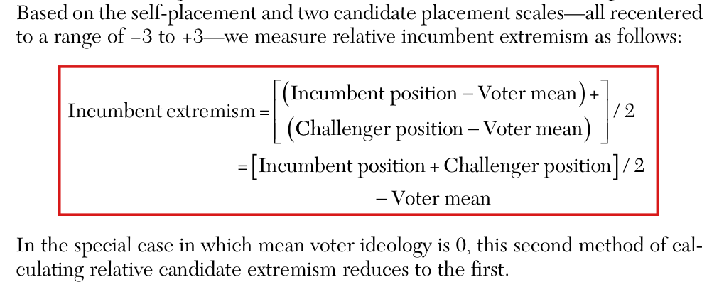(S3) Relative candidate extremism. First method, p. 132 (PDF p. 7): “On both the ANES/Rosenstone and the NOMINATE measures of ideological location, liberal positions are scored as negative and conservative positions are scored as positive. […] To do this, we first transform our scale so that positive numbers represent incumbent-party candidates’ ideology (rather than conservative candidates’ ideology), and negative numbers represent challenging-party candidates’ ideology (rather than liberal candidates’ ideology).$^{11}$ Then we take the midpoint between each set of opposing candidates to arrive at a single relative candidate extremism score for each election. With this transformed scale, positive values of our relative candidate extremism variable indicate that the incumbent-party candidate is more extreme than the challenger; negative values indicate that the challenger is more extreme than the incumbent.” (the last sentence runs on to p. 133). Note 11, p. 141 (PDF p. 16): “11. This simply involves taking the absolute value of every candidate’s ideological location score and then multiplying challenging-party candidates’ scores by −1.” Second method, p. 133 (PDF p. 8): “Based on the self-placement and two candidate placement scales—all recentered to a range of −3 to +3—we measure relative incumbent extremism as follows: $$\text{Incumbent extremism} = \left[\begin{array}{l}(\text{Incumbent position} - \text{Voter mean}) + \\ (\text{Challenger position} - \text{Voter mean})\end{array}\right] / 2 = [\text{Incumbent position} + \text{Challenger position}] / 2 - \text{Voter mean}$$ In the special case in which mean voter ideology is 0, this second method of calculating relative candidate extremism reduces to the first.” Five measures, pp. 133–134 (PDF pp. 8–9): “From the ANES data, we can calculate zero-centered and voter-centered relative candidate extremism measures for elections from 1972 to 2012. We can also calculate a zero-centered measure of relative NOMINATE extremism, but lacking a measure of voter location on the NOMINATE scale, we cannot build a voter-centered NOMINATE measure. We thus arrive at five measures of relative incumbent extremism, each of which can be tested in the musical chairs and bread and peace models. […] In testing five measures in each of the two models, we have a total of ten tests of voter sensitivity to extreme candidates in presidential elections.” [The display is the subject of clarity note P039-A001 and is not a target. 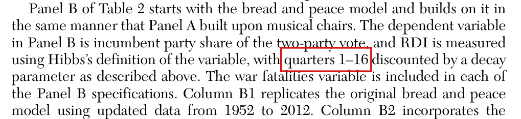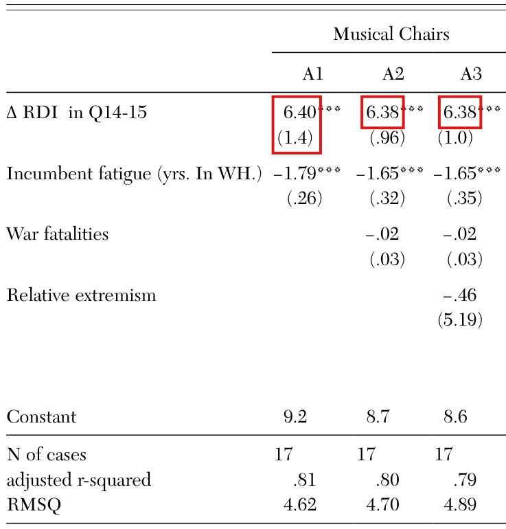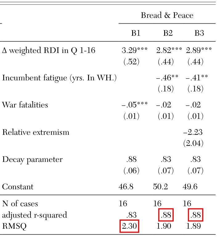The score that was computed, and that the targets use, is $(|x_I - m| - |x_C - m|)/2$, where $x_I$ and $x_C$ are the locations of the incumbent-party and challenging-party candidates on the liberal-negative, conservative-positive scale and $m$ is the reference point, 0 or the mean voter self-placement (deposited script 3).] (S4) The six specifications of Table 2. p. 136 (PDF p. 11): “Panel A of Table 2 uses the musical chairs model as a starting point. The dependent variable is incumbent party vote margin, and RDI is measured using the musical chairs version of the variable: change in RDI per capita immediately prior to the election (quarters 14 and 15). Incumbent party fatigue, measured by the number of years the incumbent party has spent in the White House, is also included in each of the specifications in Panel A. Column A1 replicates the original musical chairs model, with updated data from 1948 to 2012. Column A2 creates a composite model by introducing the war fatalities variable from bread and peace into the original musical chairs model. In column A3, we add our main incumbent party relative candidate extremism variable (the zero-centered, refined ANES/Rosenstone measure) to the composite model built in column A2.” “Panel B of Table 2 starts with the bread and peace model and builds on it in the same manner that Panel A built upon musical chairs. The dependent variable in Panel B is incumbent party share of the two-party vote, and RDI is measured using Hibbs’s definition of the variable, with quarters 1–16 discounted by a decay parameter as described above. The war fatalities variable is included in each of the Panel B specifications. Column B1 replicates the original bread and peace model using updated data from 1952 to 2012. Column B2 incorporates the incumbent fatigue variable from musical chairs to create a composite based on the bread and peace model. 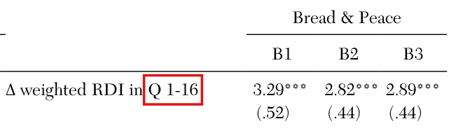Column B3 then adds our main extremism variable to the composite model from column B2.” Table 2, “Relative Extremism Variable in Baseline Models”, p. 137 (PDF p. 12; printed sideways), as printed, each coefficient followed by its parenthesized entry. Musical Chairs, columns A1 | A2 | A3: “∆ RDI in Q14-15”: 6.40*** (1.4) | 6.38*** (.96) | 6.38*** (1.0). “Incumbent fatigue (yrs. In WH.)”: −1.79*** (.26) | −1.65*** (.32) | −1.65*** (.35). “War fatalities”: blank | −.02 (.03) | −.02 (.03). “Relative extremism”: blank | blank | −.46 (5.19). “Constant”: 9.2 | 8.7 | 8.6. “N of cases”: 17 | 17 | 17. “adjusted r-squared”: .81 | .80 | .79. “RMSQ”: 4.62 | 4.70 | 4.89. Bread & Peace, columns B1 | B2 | B3: “∆ weighted RDI in Q 1-16”: 3.29*** (.52) | 2.82*** (.44) | 2.89*** (.44). “Incumbent fatigue (yrs. In WH.)”: blank | −.46** (.18) | −.41** (.18). “War fatalities”: −.05*** (.01) | −.02 (.01) | −.02 (.01). “Relative extremism”: blank | blank | −2.23 (2.04). “Decay parameter”: .88 (.06) | .83 (.07) | .83 (.07). “Constant”: 46.8 | 50.2 | 49.6. “N of cases”: 16 | 16 | 16. “adjusted r-squared”: .83 | .88 | .88. “RMSQ”: 2.30 | 1.90 | 1.89. “NOTE: Dependent variable for musical chairs is incumbent vote margin. Dependent variable for bread and peace is incumbent vote share. RDI = real disposable income; WH = White House; RMSQ = Root mean squared error. ***$p$ < .01. **$p$ < .05. *$p$ < .10.” (S5) Residual plots. p. 138 (PDF p. 13): “The residuals from the composite models in columns A2 and B2 represent the variation in vote outcomes that remains unexplained by the three fundamental variables: change in RDI, incumbent fatigue, and war fatalities. Figure 4 plots the residuals from these two composite models against our main relative extremism variable. This provides a picture of how much of the unexplained variance in vote outcomes might be explained by candidate extremism.” Figure 4, “Additional Explanatory Force of Relative Candidate Extremism” (p. 138): two panels, “Musical Chairs composite model” (vertical axis “Vote margin residuals”) and “Bread and Peace composite model” (vertical axis “Vote share residuals”), each plotting election labels against relative incumbent party candidate extremism on the horizontal axis, with a straight line drawn through the points. (S6) Maximum effects. p. 139 (PDF p. 14): “Table 3 reports the maximum effect of candidate extremism that would be predicted by each of our ten models. All estimates are based on regressions identical in form to those in columns A3 and B3 in Table 2 and fully documented in our replication files. Maximum effect is calculated as the coefficient for the variable × the largest value of that variable.” Table 3, “Maximum Effect Sizes for All Models”, p. 139, as printed, each row giving Maximum effect, Two-tailed $p$-value, $df$ for Musical chairs and then for Bread and peace: “All-voter perception measures”, “(1) Zero-centered”: −0.43, 0.90, 12 | 1.24, 0.39, 10; “(2) Voter-centered”: 1.33, 0.60, 6 | 0.30, 0.85, 5; “Refined voter perception measures”, “(3) Zero-centered”: 0.29, 0.93, 12 | 1.38, 0.30, 10; “(4) Voter-centered”: 2.28, 0.42, 6 | 0.82, 0.64, 5; “(5) NOMINATE locations”: −2.53, 0.69, 3 | 1.14, 0.77, 2. (S7) Not in the paper. The paper does not say how the models are estimated, does not say what the parenthesized entries of Table 2 are, prints no formula for the weighted income variable and prints no election-level data. These are taken from the deposited replication files (Yale Dataverse 10.60600/YU/PPBAY4, V1.1; staged under staged/code/yale-dataverse-PPBAY4-v1.1/): script 5_Tables1-3_public.R fits Panel A by lm (ordinary least squares, lines 149, 154, 159) and Panel B and the bread and peace half of Table 3 by nls (nonlinear least squares, lines 236, 242, 247, 321, 332, 343, 354, 365); script 6_Figures1-4_public.R draws each line of Figure 4 by lm(resid(file) ~ extremism) (lines 162 and 194); the relative-extremism scores are in ideology_scores_IncPtyCandRelXtrm.csv and ideology_scores_IPCRE-NOMINATE.csv and the regression inputs in data_fig3&4.csv. Where a target uses deposited numbers, each decimal string is taken as the exact rational it denotes, and the numbers are taken as given: no target concerns how the data were constructed. The online appendix cited in note 7 is not staged. 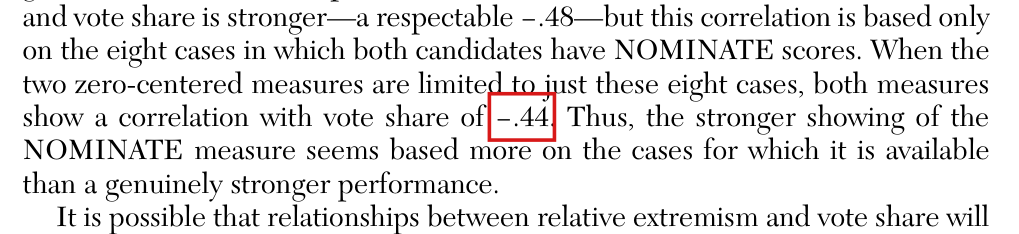Scope of the targets. None of the headline claims P039-H1 to P039-H8 is a mathematical statement (each is an empirical estimate or an interpretive conclusion), so there is no headline_result target. No finding is rated above Minor (nine confirmed errors, all Minor), so there is no result_touched_by_finding target and every target has priority 3. The seven targets come from the four confirmed errors whose correction changes mathematical content: P039-E001 (the quarter range and exponent range of the discounted income variable: a formula described with sixteen terms and fitted with fifteen, with an exact witness), P039-E002 (a significance statement read off a regression of residuals: an inferential claim that rests on an exact linear counterexample), P039-E004 (the rule “coefficient × the largest value” and the election that note 15 says it selects: the rule as worded and its stated outcome both fail on the deposited scores) and P039-E003 (a standard error in Table 2 that is arithmetically incompatible with the neighbouring printed entries). The other confirmed errors are not targets because their corrections change no mathematical statement. P039-N006 (one in-text correlation, −.44 for −.45), P039-N008 (three fit statistics in Table 2, Panel B, off by one in the last digit) and P039-N010 (two candidate locations in the worked example of p. 139, 1.58 and −.34 for 1.57 and −.33) are recalculations of reported numbers from the deposited data; the arithmetic of the worked example, $(|-.34| - |1.58|)/2 = -.62$ and $-2.23 \times (-.62) = 1.3826$, holds for the printed pair, and $(|-.33| - |1.57|)/2 = -.62$ for the corrected pair. P039-E008 and P039-N013 are bibliographic. Findings classed as clarity notes (P039-E005, P039-E006, P039-A001, P039-N005), as not confirmed or as undetermined are outside the brief; two of them touch formulas quoted above (P039-E006: note 5’s “equal weight of 1” at $\lambda = 1$; P039-A001: the display on p. 133), and the targets below do not assert the wording those notes question.

Effective claim (source TeX): Exact refutation of the printed description (the validators' witnesses; not in the paper): the income variable that the text describes gives weight to all sixteen quarters of the term, and the income variable of the fitted models gives weight zero to quarter 1; the two are different functions of the quarterly growth rates. Notation (not in the paper). For a real $\lambda \ge 0$ and reals $h_1, \dots, h_{16}$ ($h_q$ is RDI growth in quarter $q$ of the presidential term; quarter 16 is the election quarter), with the convention $\lambda^0 = 1$ also at $\lambda = 0$, put $$N_{2:16}(\lambda,h) = \tfrac13 h_{16} + \sum_{k=1}^{14} \lambda^k h_{16-k}, \qquad D_{2:16}(\lambda) = \tfrac13 + \sum_{k=1}^{14} \lambda^k, \qquad G_{2:16} = \frac{N_{2:16}}{D_{2:16}},$$ $$N_{1:16}(\lambda,h) = \tfrac13 h_{16} + \sum_{k=1}^{15} \lambda^k h_{16-k}, \qquad D_{1:16}(\lambda) = \tfrac13 + \sum_{k=1}^{15} \lambda^k, \qquad G_{1:16} = \frac{N_{1:16}}{D_{1:16}}.$$ $N_{1:16}$ is the weighted sum of the printed description: weight $\tfrac13\lambda^0$ on quarter 16 and $\lambda^{16-q}$ on quarter $q$ for $q = 15, 14, \dots, 1$ (“quarters 1–16”; exponents $0, \dots, 15$ as in note 5). $G_{2:16}$ is the expression that multiplies the income coefficient in every bread and peace model of the deposited scripts. [That the fitted models use $G_{2:16}$ is a premise read from the deposited code; it is not part of the formal statement.] (i) [The fitted variable ignores quarter 1] $N_{2:16}$, $D_{2:16}$ and $G_{2:16}$ do not depend on $h_1$: if $h$ and $h'$ agree in coordinates $2, \dots, 16$, then $G_{2:16}(\lambda,h) = G_{2:16}(\lambda,h')$. (ii) [The described variable does not ignore it] $N_{1:16}(\lambda,h) - N_{2:16}(\lambda,h) = \lambda^{15} h_1$ and $D_{1:16}(\lambda) - D_{2:16}(\lambda) = \lambda^{15}$. (iii) [Witness] Take $\lambda = \tfrac12$, $h_1 = 1$ and $h_2 = \dots = h_{16} = 0$. Then $N_{2:16} = 0$ and $G_{2:16} = 0$, while $N_{1:16} = 2^{-15} = \tfrac{1}{32768}$, $D_{1:16} = \tfrac13 + \tfrac{32767}{32768} = \tfrac{131069}{98304}$ and $G_{1:16} = \tfrac{3}{131069} > 0$. So the two variables differ, with or without the normalizing denominator. (iv) [Second witness, at a decay close to the fitted values] With $\lambda = \tfrac{9}{10}$ and the same $h$: $N_{2:16} = 0$ and $G_{2:16} = 0$, while $N_{1:16} = \big(\tfrac{9}{10}\big)^{15} = \tfrac{205891132094649}{10^{15}}$, $D_{1:16} = \tfrac{22440939433444477}{3 \cdot 10^{15}}$ and $G_{1:16} = \tfrac{617673396283947}{22440939433444477} > 0$.

: T1Statement

Theorem: SAP.P039.T1

Statement hash: bdf8c71a29d919842eda9ecdcffae478298aa730086de4707ef1279c7999721e

Statement definition: SAP.P039.T1Statement

Certificate. 20261104T174956Z

Declaration review: faithful; 2026-11-04T18:28:14Z; binding v2

Evidence scope: Certification checks formal proof objects. Statement fidelity is a model judgment. Author review is separate.

Proof dependencies: Independently extracted

Source and evidence metadata · sap-2026-11-08-assured-release

P039-T2

The description of the bread and peace income variable (p. 128, p. 136, the Table 2 row label and note 5), corrected: quarters 2–16, with exponents 0 to 14

p. 136 (PDF p. 11); Table 2, p. 137 (PDF p. 12); p. 128 (PDF p. 3); note 5, p. 141 (PDF p. 16)

pp. 128, 136--137 and note 5, p. 141. The corrected Q2--16 predictor has positive normalization, ignores quarter one, and satisfies the exact difference, equality characterization and endpoint formulas.

Historical component credits

Proved AronowAudit.P039.income_denominators_positive Historical support retained; baseline fidelity: ok; manifest: used; used in Solution; Fidelity sweep: ok
Proved AronowAudit.P039.income_growth_difference Historical support retained; baseline fidelity: ok; manifest: used; used in Solution; Fidelity sweep: ok
Proved AronowAudit.P039.income_growth_equality_iff Historical support retained; baseline fidelity: ok; manifest: used; used in Solution; Fidelity sweep: ok
Proved AronowAudit.P039.income_endpoint_values Historical support retained; baseline fidelity: ok; manifest: used; used in Solution; The powers are asserted for all natural exponents, which includes the target exponents 0–14. Quarter 16 retains its factor 1/3 at unit decay, as the corrected target requires.

Formal result: whole

Formal statement · Proof · Definitions

Assumptions and verification

Claim revision: catalog:28d65528e235778b86f5d033b5bc6c8a730ed2a55d78c195a655539f232f795f

Effective claim (source TeX): Sol's repair (validated.json, P039-E001, smallest_repair), verbatim: “Explicitly disclose that these analyses exclude Q1 and use Q2–16; change the quarter range on p. 136 and the Table 2 Bread & Peace row label to 2–16; clarify the implemented range in the p. 128 discussion. If note 5 describes this implementation, end its power sequence at 14 instead of 15. This preserves the fitted results. Alternatively, implement the originally stated Q1–16 predictor by adding lambda^15*h1 to the numerator and lambda^15 to the denominator in all nine formulas, then refit and update Table 2B, the Bread & Peace half of Table 3, Figure 4B, and the numerical discussion; remove B3 fatigue's p<.05 marker.” Corrected text (validated.json, prior_correction.corrected_text, first alternative): “In the analyses reported here, the weighted income-growth predictor uses quarters 2–16 of each presidential term; quarter 1 is excluded. Quarter 16 receives weight 1/3, quarters 15 through 2 receive weights lambda through lambda^14, and the weighted sum is divided by 1/3+sum_{k=1}^{14}lambda^k. Label the Table 2 Bread & Peace income row 'Delta weighted RDI in Q 2-16.'” Mathematical content, with every hypothesis. Notation as in P039-T1: $\lambda \ge 0$ real, $h = (h_1, \dots, h_{16}) \in \mathbb{R}^{16}$, $\lambda^0 = 1$ also at $\lambda = 0$. (i) [Corrected definition] The income variable of the fitted models is $$G_{2:16}(\lambda,h) = \frac{\tfrac13 h_{16} + \sum_{k=1}^{14} \lambda^k h_{16-k}}{\tfrac13 + \sum_{k=1}^{14} \lambda^k},$$ with weight $\tfrac13$ on quarter 16, weight $\lambda^{16-q}$ on quarter $q$ for $q = 15, \dots, 2$ (exponents 1 to 14) and no weight on quarter 1. For every $\lambda \ge 0$ the denominator satisfies $D_{2:16}(\lambda) \ge \tfrac13 > 0$, so $G_{2:16}(\lambda,h)$ is defined, and it does not depend on $h_1$. (ii) [Exact relation to the sixteen-quarter variable of the printed description] For every $\lambda \ge 0$ and every $h$: $N_{1:16} = N_{2:16} + \lambda^{15} h_1$, $D_{1:16} = D_{2:16} + \lambda^{15}$, and $$G_{1:16}(\lambda,h) - G_{2:16}(\lambda,h) = \frac{\lambda^{15}\,\big(h_1 - G_{2:16}(\lambda,h)\big)}{D_{1:16}(\lambda)}.$$ Hence $G_{1:16}(\lambda,h) = G_{2:16}(\lambda,h)$ if and only if $\lambda = 0$ or $h_1 = G_{2:16}(\lambda,h)$. (iii) [The two limiting cases of note 5, with the exponents running from 0 to 14] At $\lambda = 1$: $1^{14} = 1^{13} = \dots = 1^0 = 1$, the weights are $\tfrac13$ on quarter 16 and $1$ on each of quarters $15, \dots, 2$, $D_{2:16}(1) = \tfrac{43}{3}$ and $G_{2:16}(1,h) = \tfrac{3}{43}\big(\tfrac13 h_{16} + \sum_{q=2}^{15} h_q\big)$. At $\lambda = 0$: $0^{14} = \dots = 0^1 = 0$ and $0^0 = 1$, every quarter before the election quarter has weight 0, $D_{2:16}(0) = \tfrac13$ and $G_{2:16}(0,h) = h_{16}$.

: T2Statement

Theorem: SAP.P039.T2

Statement hash: c4f8ecb738b7bc98ac5ece100ee0012be5f5036d37c5563bc07d9200f25ca94c

Statement definition: SAP.P039.T2Statement

Certificate. 20261104T174956Z

Declaration review: faithful; 2026-11-04T18:28:14Z; binding v2

Evidence scope: Certification checks formal proof objects. Statement fidelity is a model judgment. Author review is separate.

Proof dependencies: Independently extracted

Source and evidence metadata · sap-2026-11-08-assured-release

P039-T3

p. 138, last sentence, with Figure 4, panel B: the two-tailed p-value of the line fitted to the B2 residuals (.26), read as a test of the statistical significance of candidate extremism once the fundamentals are accounted for; the witness is the validator's construction and is not in the paper

p. 138 (PDF p. 13), last sentence, and Figure 4, panel B; compare Table 2, column B3 (p. 137, PDF p. 12) and Table 3, row (3) (p. 139, PDF p. 14)

Figure 4 and p. 138, compared with Table 2, p. 137 and Table 3, p. 139. The six-observation OLS witnesses give different tests at 5%, different slopes for the correlated regressor, and the stated Gaussian-null scaled-t3 law and moments. For every nonnegative threshold the two analytic formulas are the actual t4 and t3 two-sided probability tails. The intermediate square and arctangent comparisons and four-decimal p-value enclosures hold. The usual measure-theoretic conditions are assumed; statistics are totalized on the Gaussian null set of zero SSE.

Historical component credits

Proved AronowAudit.P039.squaredLength_nonnegative Historical support retained; baseline fidelity: ok; manifest: used; used in Solution; Auxiliary nonnegativity is used inside the existing fit proofs and is not a claim component.
Proved AronowAudit.P039.squaredLength_zero_iff Historical support retained; baseline fidelity: ok; manifest: used; used in Solution; Auxiliary zero-criterion lemma is used inside existing uniqueness proofs.
Proved AronowAudit.P039.normal_equation_expansion Historical support retained; baseline fidelity: ok; manifest: used; used in Solution; Auxiliary SSE expansion is already used inside the exported least-squares fits.
Proved AronowAudit.P039.normal_equation_unique Historical support retained; baseline fidelity: ok; manifest: used; used in Solution; Auxiliary normal-equation uniqueness is already included in each concrete witness fit.
Proved AronowAudit.P039.gram_certificate_full_rank Historical support retained; baseline fidelity: ok; manifest: used; used in Solution; Auxiliary Gram-certificate lemma is already used inside the exported concrete fits; no separate helper assertion is included.
Proved AronowAudit.P039.witness_baseline Historical support retained; baseline fidelity: ok; manifest: used; used in Solution; Baseline component of target (i). Its extra inverse-Gram and coefficient equalities support, rather than restrict, the specified first-stage calculation. No claim-stage verdict changed after reading the record.
Proved AronowAudit.P039.witness_residual_projection Historical support retained; baseline fidelity: ok; manifest: used; used in Solution; Projection component of target (i); combined with R231-15, the final identity gives the exact residual vector and its squared length. No claim-stage verdict changed after reading the record.
Proved AronowAudit.P039.residual_test_five_percent_disagreement Historical support retained; baseline fidelity: ok; manifest: used; used in Solution; Auxiliary analytic-tail calculation for target (iii); this row does not claim the fitted t identities, which R231-07 supplies, or a measure-theoretic derivation of the closed forms. The target itself gives these exact closed forms, so their use as representations changes no covered value. No claim-stage verdict changed after reading the record.
Proved AronowAudit.P039.residual_orthogonal_witness_fit Historical support retained; baseline fidelity: ok; manifest: used; used in Solution; Witness-fit component of target (ii); the conventional variance denominator is 6−2=4, rather than the full model’s 6−3=3. No claim-stage verdict changed after reading the record.
Proved AronowAudit.P039.full_orthogonal_witness_fit Historical support retained; baseline fidelity: ok; manifest: used; used in Solution; Witness-fit component of target (ii); together with R231-11 it gives the same slope and residuals but different conventional squared t values. No claim-stage verdict changed after reading the record.
Proved AronowAudit.P039.residual_correlated_witness_fit Historical support retained; baseline fidelity: ok; manifest: used; used in Solution; Witness-fit component of target (iv); its full-rank, unique-fit and positive-SE conclusions establish the stated calculation rather than assuming it. No claim-stage verdict changed after reading the record.
Proved AronowAudit.P039.full_correlated_witness_fit Historical support retained; baseline fidelity: ok; manifest: used; used in Solution; Witness-fit component of target (iv), not a standalone refutation of every part of T3. No claim-stage verdict changed after reading the record.
Counterexample proved AronowAudit.P039.regression_procedure_counterexample Historical support retained; baseline fidelity: ok; manifest: used; used in Solution; Exact witness against identifying the two OLS procedures: the target expressly chooses six observations and permits different tested regressors for its statistic and slope discrepancies. This is not a refutation of the numerical .26 on the empirical sample. No claim-stage verdict changed after reading the record.
Proved AronowAudit.P039.correlated_regressor_residual_ratio Historical support retained; baseline fidelity: ok; manifest: used; used in Solution; Auxiliary ratio calculation for target (iv): the final equality uses numerical slope values; R231-09 and R231-02 separately identify those numbers with the actual residual and full-model slopes. No claim-stage verdict changed after reading the record.
Counterexample proved AronowAudit.P039.regression_five_percent_counterexample Historical support retained; baseline fidelity: ok; manifest: used; used in Solution; The two nominal p-values are represented by the exact analytic formulas printed in target (iii). This statement does not additionally identify them with tail events of studentLaw; no numerical case or test decision covered by this row is lost. The counterexample concerns the OLS procedure, not the literal .26 output on the paper’s nonlinear data. No claim-stage verdict changed after reading the record.
Counterexample proved AronowAudit.P039.residual_gaussian_reference_counterexample Historical support retained; baseline fidelity: ok; manifest: used; used in Solution; Positive σ in ℝ≥0 represents every positive real scale in the target. Total division extends the statistic by zero on zero-SSE outcomes, a Gaussian null event, so the law and moments retain their usual meaning. All three asserted second moments are nonzero, hence cannot arise from the Bochner integral’s nonintegrable-value-zero convention. No claim-stage verdict changed after reading the record.

Formal result: whole

Formal statement · Proof · Definitions

Assumptions and verification

Claim revision: catalog:933978dd7a738add431b6776e8ab4be1535c8357d5c1a7523acb8a3aff19e93b

Effective claim (source TeX): Exact refutation of the procedure (the validator's witness; not in the paper): the ordinary $t$ test of the slope in a regression of first-stage residuals on a raw regressor, referred to $n - 2$ degrees of freedom, is not the test of that regressor's coefficient in the model that also contains the first-stage regressors. On the same data the two tests can disagree at the 5% level, the two slopes can differ, and under the Gaussian null the residual-regression statistic does not have the $t_{n-2}$ distribution. Setting (ordinary least squares, conventional standard errors). For a design matrix $A$ with $n$ rows and full column rank $p$ and a response $c \in \mathbb{R}^n$: $\hat\beta = (A^\top A)^{-1} A^\top c$, $\mathrm{SSE} = \|c - A\hat\beta\|^2$, degrees of freedom $n - p$, squared standard error of the last coefficient $\mathrm{SE}^2 = \frac{\mathrm{SSE}}{n-p}\,\big[(A^\top A)^{-1}\big]_{pp}$, and $t = \hat\beta_p / \mathrm{SE}$. Let $n = 6$, $\mathbf{1} = (1,1,1,1,1,1)^\top$, $u = (1,-1,0,0,0,0)^\top$, $v = (0,0,1,-1,0,0)^\top$, $w = (0,0,0,0,1,-1)^\top$; first-stage design $Z = [\mathbf{1}, u]$; $M = I - Z(Z^\top Z)^{-1} Z^\top$; outcome $y = u + \tfrac32 v + w = (1, -1, \tfrac32, -\tfrac32, 1, -1)^\top$; first-stage residual $r = My$. (i) $Z^\top Z = \mathrm{diag}(6, 2)$, $M$ is symmetric and idempotent of rank 4, $r = \tfrac32 v + w = (0, 0, \tfrac32, -\tfrac32, 1, -1)^\top$ and $\|r\|^2 = \tfrac{13}{2}$. (ii) [Same slope and same residuals, different tests] Take $x = v$. Residual regression (response $r$, design $[\mathbf{1}, x]$): coefficients $(0, \tfrac32)$, residual vector $w$, $\mathrm{SSE} = 2$, 4 degrees of freedom, $\mathrm{SE}^2 = \tfrac14$, $t^2 = 9$. Full regression (response $y$, design $[\mathbf{1}, u, x]$): coefficients $(0, 1, \tfrac32)$, residual vector $w$, $\mathrm{SSE} = 2$, 3 degrees of freedom, $\mathrm{SE}^2 = \tfrac13$, $t^2 = \tfrac{27}{4}$. (iii) [The two tests disagree at the 5% level] For $t \ge 0$ the two-sided tail probability of Student's $t_4$ is $1 - \tfrac32 z + \tfrac12 z^3$ with $z = t/\sqrt{4 + t^2}$; at $t = 3$ it is $p_{\mathrm{res}} = 1 - \frac{45}{13\sqrt{13}}$, and $p_{\mathrm{res}} < \tfrac{1}{20}$ because $900 > 247\sqrt{13}$, that is $900^2 = 810000 > 793117 = 247^2 \cdot 13$. For $t \ge 0$ the two-sided tail probability of Student's $t_3$ is $1 - \frac{2}{\pi}\big(\arctan q + \frac{q}{1+q^2}\big)$ with $q = t/\sqrt{3}$; at $t = \tfrac{3\sqrt3}{2}$ (so $q = \tfrac32$, and $\arctan\tfrac32 = \tfrac{\pi}{4} + \arctan\tfrac15$) it is $p_{\mathrm{full}} = \tfrac12 - \frac{2}{\pi}\big(\arctan\tfrac15 + \tfrac{6}{13}\big)$, and $p_{\mathrm{full}} > \tfrac12 - \tfrac23\big(\tfrac15 + \tfrac{6}{13}\big) = \tfrac{23}{390} > \tfrac{1}{20}$ because $\arctan\tfrac15 < \tfrac15$ and $\pi > 3$. So the test of the line through the residuals rejects at the 5% level and the test of the coefficient in the full model does not ($p_{\mathrm{res}} \approx .0399$, $p_{\mathrm{full}} \approx .0805$). (iv) [The slopes differ when the raw regressor is correlated with a first-stage regressor] Take instead $x = u + v$, with the same $Z$, $y$ and $r$. Residual regression of $r$ on $[\mathbf{1}, x]$: slope $\tfrac34$, $\mathrm{SSE} = \tfrac{17}{4}$, $t^2 = \tfrac{36}{17}$ on 4 degrees of freedom. Full regression of $y$ on $[\mathbf{1}, u, x]$: coefficients $(0, -\tfrac12, \tfrac32)$, so the coefficient of $x$ is $\tfrac32$, with $\mathrm{SSE} = 2$ and $t^2 = \tfrac{27}{4}$ on 3 degrees of freedom. Here $x^\top M x = 2$, $x^\top x = 4$ and $\tfrac34 = \tfrac32 \cdot \tfrac24$. (v) [Wrong reference distribution under the null] Let $x = v$ and $y = Z\gamma + \varepsilon$ with $\gamma \in \mathbb{R}^2$ and $\varepsilon \sim N(0, \sigma^2 I_6)$, $\sigma > 0$. Then the residual-regression statistic is $T_{\mathrm{res}} = U/\sqrt{V/4}$, where $U = v^\top\varepsilon/(\sigma\sqrt2) \sim N(0,1)$ and $V \sim \chi^2_3$ is independent of $U$; that is, $T_{\mathrm{res}} = \sqrt{4/3}\;T$ with $T \sim t_3$. Hence $E[T_{\mathrm{res}}^2] = \tfrac43 \cdot 3 = 4$, whereas a $t_4$ variable has second moment $\tfrac{4}{4-2} = 2$: $T_{\mathrm{res}}$ is not $t_4$ distributed.

: SAP.P039.T3WholeStatement

Theorem: SAP.P039.T3

Statement hash: 0f3a5df1b63a9df43e4f9f354a195bfcaadc6a65450b9a70e1a0f6a3f82aceb0

Statement definition: SAP.P039.T3WholeStatement

Certificate. 20261104T174956Z

Declaration review: faithful; 2026-11-04T18:28:14Z; binding v2

Evidence scope: Certification checks formal proof objects. Statement fidelity is a model judgment. Author review is separate.

Proof dependencies: Independently extracted

Manifest annotation reconciliation: Effective use follows the source-bound dependency observation; original annotations are retained in the crosswalk.

AronowAudit.P039.gram_certificate_full_rank: observed used

AronowAudit.P039.normal_equation_expansion: observed used

AronowAudit.P039.normal_equation_unique: observed used

AronowAudit.P039.squaredLength_nonnegative: observed used

AronowAudit.P039.squaredLength_zero_iff: observed used

Source and evidence metadata · sap-2026-11-08-assured-release

P039-T4

p. 138, last sentence, as repaired by Sol: the line of Figure 4, panel B is descriptive, and the test of extremism given the fundamentals is the test of its coefficient in the full model B3 (formal content: the algebra that relates the two regressions)

p. 138 (PDF p. 13), last sentence

p. 138, final sentence, with the exact linear-OLS interpretation. For every full-rank control design containing an intercept and every additional regressor outside its span, clauses (a)--(e) give the projection, attenuation, SE and t identities. Under positive isotropic noise the residual covariance has rank n-k. Under the Gaussian null the full statistic has the central t(n-k-1) law; an orthogonal centered regressor gives the stated scaled residual-line law, which differs from t(n-2) when k is at least two, including residual df one or two. The usual measure-theoretic conditions are assumed. The empirical nonlinear application in (g) is expressly outside the formal claim.

Historical component credits

Proved AronowAudit.P039.full_rank_gram_unit Historical support retained; baseline fidelity: ok; manifest: used; used in Solution; Auxiliary Gram invertibility is already incorporated in corrected_residual_regression.
Proved AronowAudit.P039.ols_projection_identities Historical support retained; baseline fidelity: ok; manifest: used; used in Solution; The projection identities are already part of corrected_residual_regression.
Proved AronowAudit.P039.full_rank_ols_unique Historical support retained; baseline fidelity: ok; manifest: used; used in Solution; The needed uniqueness is already part of corrected_residual_regression.
Proved AronowAudit.P039.residual_attenuation_algebra Historical support retained; baseline fidelity: ok; manifest: used; used in Solution; Its attenuation and SSE conclusions are already included in corrected_residual_regression.
Proved AronowAudit.P039.residual_t_squared_algebra Historical support retained; baseline fidelity: ok; manifest: used; used in Solution; Its guarded squared-t conclusions are already included in corrected_residual_regression.
Proved AronowAudit.P039.corrected_residual_regression Historical support retained; baseline fidelity: ok; manifest: used; used in Solution; Fidelity sweep: ok
Proved AronowAudit.P039.PaperDomains.corrected_residual_covariance_assessment Historical support retained; baseline fidelity: ok; manifest: used; used in Solution; {'source': 'adjudication+second review', 'adjudicator': 'P039/P039_PaperInstances.lean:61 adds the outer hypothesis hσ : 0 < σ, so the residual and covariance identities and the covariance rank/non-identity conclusions at lines 73–76 all require positive noise, whereas the first sentence of T4(f) asserts them from Eε = 0 and Cov(ε) = σ²I without that restriction. For n = 6, k = 2, Z = [1, (1,−1,0,0,0,0)], x = (0,0,1,−1,0,0), γ = 0 and ε = 0 on a one-point probability space, σ = 0 satisfies the target assumptions, but Cov(r) = 0 has rank 0 rather than 4 and equals σ²I; the excluded case falsifies substantive target conclusions, rather than merely leaving an easy true boundary case unproved. The additional negation of LiteralCovarianceClaim at P039/P039_PaperInstances.lean:80 correctly identifies this false target subclaim but does not establish it or supply the valid zero-noise identities from the credited declaration. The Student-law premise at P039/P039_PaperInstances.lean:77 is explicitly permitted by record.json’s T4 note, so the reviewer’s withdrawn objection to that premise is rejected. The necessary correction concerns the audit’s formal T4(f), whose unguarded rank/non-identity assertion is absent from the supplied empirical paper correction.', 'suggested_fix': 'Add σ > 0 to the first covariance premise of the formal target T4(f), and record this as an additional correction to the validator’s formal claim; this makes the credited positive-noise assessment faithful without changing the empirical replacement sentence. If the target is to retain its valid covariance identities for σ = 0, leave those identities unconditional, place the positive-noise guard only on covariance rank/non-identity, and use P039/P039_Regression.lean:1744 (corrected_residual_covariance_and_law) as the corresponding credited declaration.', 'second_review': 'T4(f) says Cov(r) = σ²M is “a matrix of rank n − k and not σ²I_n” without a positive-noise premise, whereas vectorCovariance is the ordinary centered-integral covariance matrix (P039/P039_Regression.lean:1545). At σ = 0 with zero noise, n = 6, k = 2, Z = [1, (1,−1,0,0,0,0)] and x = (0,0,1,−1,0,0), the target assumptions hold but Cov(r) = 0 has rank 0 rather than 4 and equals σ²I_n; P039/P039_PaperInstances.lean:10 defines precisely this unguarded rank/non-identity claim, refuted at line 37. The credited theorem explicitly requires hσ : 0 < σ (P039/P039_PaperInstances.lean:61), so the substantive error is in the audit’s formal correction, not in an empirical covariance assertion from the paper. Correct T4(f) by guarding rank/non-identity with σ > 0; if its valid zero-noise identities are retained, use P039/P039_Regression.lean:1744, which exports those identities unconditionally and guards only rank/non-identity.', 'severity': None}

Formal result: whole

Formal statement · Proof · Definitions

Assumptions and verification

Claim revision: CT-02:P039-T4:accepted

Effective claim (source TeX): Sol's repair (validated.json, P039-E002, smallest_repair), verbatim: “Keep Figure 4B as a descriptive residual plot. Replace the significance sentence with: 'The negative slope in panel B is descriptive. In the full bread and peace composite model B3, the extremism coefficient is -2.23, with an approximate two-tailed p-value of .30 on ten degrees of freedom; it remains well short of statistical significance.'” Formal content of the corrected claim (exact for linear least squares; the validator's derivation, steps 1–8). Let $Z$ be a real $n \times k$ matrix of full column rank whose column space contains $\mathbf{1}$, let $x \in \mathbb{R}^n$ lie outside the column space of $Z$, let $y \in \mathbb{R}^n$, and let $n > k + 1$. Put $P = Z(Z^\top Z)^{-1} Z^\top$, $M = I - P$, $r = My$ (the first-stage residual), $\bar x = \mathbf{1}^\top x / n$, $x_c = x - \bar x\,\mathbf{1}$, $S_M = x^\top M x$ and $S_c = x_c^\top x_c$. (a) $P^\top = P = P^2$, $M^\top = M = M^2$, $MZ = 0$, $\mathbf{1}^\top r = 0$, $M x_c = M x$, $x_c^\top r = x^\top r = x^\top M y$, and $S_c = S_M + \|P x_c\|^2$. Hence $0 < S_M \le S_c$, with $S_M = S_c$ if and only if $P x_c = 0$, that is, if and only if the centered regressor is orthogonal to every column of $Z$. (b) [The line through the residuals] The least-squares fit of $r$ on $[\mathbf{1}, x]$ has slope $a = x^\top r / S_c$ and intercept $-a\bar x$, and its error sum of squares is $\mathrm{SSE}_{\mathrm{res}} = \|r\|^2 - (x^\top r)^2 / S_c$. (c) [The full model] The least-squares fit of $y$ on $[Z, x]$ is unique; its coefficient on $x$ is $b = x^\top r / S_M$ and its error sum of squares is $\mathrm{SSE}_{\mathrm{full}} = \|r\|^2 - (x^\top r)^2 / S_M$. (d) [Attenuation] $a = b\,S_M / S_c$. So $a$ and $b$ have the same sign, $|a| \le |b|$, and $a = b$ if and only if $b = 0$ or $P x_c = 0$; and $\mathrm{SSE}_{\mathrm{full}} \le \mathrm{SSE}_{\mathrm{res}}$. (e) [The two $t$ statistics] With conventional standard errors, $\mathrm{SE}_{\mathrm{res}}^2 = \frac{\mathrm{SSE}_{\mathrm{res}}}{(n-2)\,S_c}$ on $n - 2$ degrees of freedom and $\mathrm{SE}_{\mathrm{full}}^2 = \frac{\mathrm{SSE}_{\mathrm{full}}}{(n-k-1)\,S_M}$ on $n - k - 1$ degrees of freedom. If $\mathrm{SSE}_{\mathrm{full}} > 0$, then $$t_{\mathrm{res}}^2 = \frac{a^2}{\mathrm{SE}_{\mathrm{res}}^2} = \frac{(n-2)\,(x^\top r)^2}{S_c\|r\|^2 - (x^\top r)^2}, \qquad t_{\mathrm{full}}^2 = \frac{b^2}{\mathrm{SE}_{\mathrm{full}}^2} = \frac{(n-k-1)\,(x^\top r)^2}{S_M\|r\|^2 - (x^\top r)^2},$$ and therefore $\frac{t_{\mathrm{res}}^2}{n-2} \le \frac{t_{\mathrm{full}}^2}{n-k-1}$. If moreover $P x_c = 0$, then $a = b$, the two fits have the same residual vector, and $t_{\mathrm{res}} = \sqrt{\frac{n-2}{n-k-1}}\;t_{\mathrm{full}}$: the same slope and the same residuals, with the error sum of squares divided by $n - 2$ in place of $n - k - 1$, so that $|t_{\mathrm{res}}| > |t_{\mathrm{full}}|$ whenever $k \ge 2$ and $t_{\mathrm{full}} \ne 0$. (f) [Why the residual line has no $t_{n-2}$ reference] If $y = Z\gamma + \varepsilon$ with $\sigma > 0$, $E\varepsilon = 0$ and $\mathrm{Cov}(\varepsilon) = \sigma^2 I_n$, then $r = M\varepsilon$ and $\mathrm{Cov}(r) = \sigma^2 M$, a matrix of rank $n - k$ and not $\sigma^2 I_n$. If in addition $\varepsilon$ is Gaussian with $\sigma > 0$, then $t_{\mathrm{full}}$ has the $t_{n-k-1}$ distribution; when $P x_c = 0$, by (e), $t_{\mathrm{res}}$ is $\sqrt{(n-2)/(n-k-1)}$ times a $t_{n-k-1}$ variable, which for $k \ge 2$ is not $t_{n-2}$ distributed (P039-T3 (v) is the case $n = 6$, $k = 2$). (g) [Application to the paper; not a formal part] In the paper $n = 16$ and the first stage B2 has five fitted parameters (constant, income coefficient, incumbent fatigue, war fatalities, decay parameter), so the line of Figure 4, panel B is referred to $n - 2 = 14$ degrees of freedom and the coefficient in B3 to $16 - 6 = 10$, the count printed in Table 3. B2 and B3 are nonlinear in the decay parameter, so (a)–(f) apply to them through the linearization at the fitted parameters, with $Z$ replaced by the $16 \times 5$ Jacobian of the B2 mean function. The corrected sentence reports the test that (c) and (e) describe: the coefficient −2.23 with standard error 2.04 in B3 and its approximate two-tailed $p$-value .30 on ten degrees of freedom.

: SAP.P039.T4WholeStatement

Theorem: SAP.P039.T4

Statement hash: c262af6cc02738f7a2979e600b753bb66adad9fd2c94d9709b305df5715d3269

Statement definition: SAP.P039.T4WholeStatement

Certificate. 20261104T174956Z

Declaration review: faithful; 2026-11-04T18:28:14Z; binding v2

Evidence scope: Certification checks formal proof objects. Statement fidelity is a model judgment. Author review is separate.

Proof dependencies: Independently extracted

Manifest annotation reconciliation: Effective use follows the source-bound dependency observation; original annotations are retained in the crosswalk.

AronowAudit.P039.full_rank_gram_unit: observed used

AronowAudit.P039.full_rank_ols_unique: observed used

AronowAudit.P039.ols_projection_identities: observed used

AronowAudit.P039.residual_attenuation_algebra: observed used

AronowAudit.P039.residual_t_squared_algebra: observed used

Source and evidence metadata · sap-2026-11-08-assured-release

P039-T5

p. 139: ‘Maximum effect is calculated as the coefficient for the variable × the largest value of that variable’ and ‘The largest value of the zero-centered refined variable occurs in 1980’; note 15: ‘For the eight measures based on ANES/Rosenstone, this was the 1980 election’; as printed. The witnesses are the validators' calculations on the deposited scores and are not in the paper

p. 139 (PDF p. 14), the two paragraphs under the heading ‘Maximum predicted effect of relative candidate extremism’; note 15, p. 142 (PDF p. 17)

p. 139 and note 15, p. 142. Both voter-centered score comparisons refute the 1980 selection, and all five signed maxima are positive, with the worked signed-maximum product negative.

Historical component credits

Proved AronowAudit.P039.signed_extremism_maxima Historical support retained; baseline fidelity: ok; manifest: used; used in Solution; This covers the literal signed-order clause T5(ii). As the target note clarifies, the printed worked example indicates a largest-magnitude intention and its positive 1.38 is not shown numerically erroneous by this lemma; the result diagnoses the wording of the rule.
Counterexample proved AronowAudit.P039.voter_centered_1980_counterexample Historical support retained; baseline fidelity: ok; manifest: used; used in Solution; Fidelity sweep: ok
Counterexample proved AronowAudit.P039.literal_largest_value_counterexample Historical support retained; baseline fidelity: ok; manifest: used; used in Solution; This covers the literal signed-order clause T5(ii). As the target note clarifies, the printed worked example indicates a largest-magnitude intention and its positive 1.38 is not shown numerically erroneous by this lemma; the result diagnoses the wording of the rule.

Formal result: whole

Formal statement · Proof · Definitions

Assumptions and verification

Claim revision: catalog:f40b5131711adf361ac27f5199da77b0b7087ed1677fdc06f94ffdcddf5a9b23

Effective claim (source TeX): Exact refutation (the validators' calculations on the deposited relative-extremism scores, taken as exact decimals; the scores are not printed in the paper). Notation. For measure $j \in \{1, \dots, 5\}$ (the rows of Table 3) and election year $t$, $x_{j,t}$ is the incumbent-party relative candidate extremism score, defined for $t \in T_j$: $T_1 = T_3 = \{1948, 1952, \dots, 2012\}$ (17 elections), $T_2 = T_4 = \{1972, 1976, \dots, 2012\}$ (11 elections) and $T_5 = \{1960, 1964, 1968, 1972, 1984, 1996, 2004, 2008\}$ (8 elections). The 64 values are listed in definitions_needed. (i) [Note 15 fails for both voter-centered measures] $x_{2,1972} = -0.51177218671487$ and $x_{2,1980} = -0.171462108121506$, so $|x_{2,1972}| - |x_{2,1980}| = \frac{85077519648341}{250000000000000} > 0$. $x_{4,1972} = -0.60215659702977$ and $x_{4,1980} = -0.294347822983647$, so $|x_{4,1972}| - |x_{4,1980}| = \frac{307808774046123}{1000000000000000} > 0$. Hence for measures (2) and (4) the score of greatest magnitude is not the 1980 score, and the four maximum effects in rows (2) and (4) of Table 3 (one for each model in each row) are not computed from the 1980 election; the statement “For the eight measures based on ANES/Rosenstone, this was the 1980 election” is false for four of the eight. (ii) [The largest value in signed order is not the value used] $x_{3,1980} = -0.621023999873778 < 0 < 0.27380029103004 = x_{3,1984}$, so the largest value of the zero-centered refined variable does not occur in 1980 and is not $-.62$. For every measure the largest value in signed order is positive: $\max_t x_{1,t} = x_{1,1984} = 0.235890938802093$, $\max_t x_{2,t} = x_{2,1996} = 0.336875932107128$, $\max_t x_{3,t} = x_{3,1984} = 0.27380029103004$, $\max_t x_{4,t} = x_{4,2012} = 0.34241131733838$ and $\max_t x_{5,t} = x_{5,1968} = 0.116$. Under the rule as worded the score “employed in these calculations” would therefore be positive for all five variables, against “always negative” in the next paragraph of p. 139; for the worked example it would give $-2.23 \times 0.27380029103004 = -\frac{1526436622492473}{2500000000000000} < 0$, not the printed $+1.38$.

: T5Statement

Theorem: SAP.P039.T5

Statement hash: d1278a217536e79e5c9da7c3856565655bfd9a551426c2d4b5a9a9c59be4c527

Statement definition: SAP.P039.T5Statement

Certificate. 20261104T174956Z

Declaration review: faithful; 2026-11-04T18:28:14Z; binding v2

Evidence scope: Certification checks formal proof objects. Statement fidelity is a model judgment. Author review is separate.

Proof dependencies: Independently extracted

Source and evidence metadata · sap-2026-11-08-assured-release

P039-T6

The maximum-effect rule of p. 139 and note 15, corrected: coefficient × the observed score of greatest absolute magnitude, with its sign; the elections selected are 1980 (zero-centered measures), 1972 (voter-centered measures) and 1964 (NOMINATE)

p. 139 (PDF p. 14); note 15, p. 142 (PDF p. 17); Table 3, p. 139

p. 139 and corrected note 15, p. 142. The corrected magnitude rule uniquely selects the stated elections with positive attained margins in both samples, gives the signed fitted contribution and its maximum magnitude, and preserves the rounded worked example.

Historical component credits

Proved AronowAudit.P039.corrected_extremism_selections Historical support retained; baseline fidelity: ok; manifest: used; used in Solution; Covers the selection, uniqueness and score-sign portions of T6(i)–(ii). The five exact selected-score equalities are also exposed by unfolding the score definition; the description does not claim that signed-order maxima occur in these years. No change from claim-stage.json after reading the record.
Proved AronowAudit.P039.corrected_extremism_margins Historical support retained; baseline fidelity: ok; manifest: used; used in Solution; Covers the exact-margin portion of corrected target T6(i). The observed sets and deposited values are fixed inputs as required by S7; no data-construction or estimation theorem is claimed. No change from claim-stage.json after reading the record.
Proved AronowAudit.P039.maximum_effect_samples Historical support retained; baseline fidelity: ok; manifest: used; used in Solution; Covers precisely T6(iii), which specifies the sample sets and the cardinality formulas for the printed degrees of freedom. Natural subtraction does not truncate here; the theorem is not credited as deriving residual degrees of freedom from a regression-rank theorem. No change from claim-stage.json after reading the record.
Proved AronowAudit.P039.maximum_effect_contribution Historical support retained; baseline fidelity: ok; manifest: used; used in Solution; Covers T6(iv) pointwise: for each covariate value z substitute g=ĝ(z) and β=β̂. The target itself is conditional on additive form in x; it does not demand estimating or validating a particular fitted model. β=0 is correctly included by a weak magnitude inequality. No change from claim-stage.json after reading the record.
Proved AronowAudit.P039.maximum_effect_sign Historical support retained; baseline fidelity: ok; manifest: used; used in Solution; Covers the product-sign clause of T6(iv). maximumEffect defines the corrected signed product, while the negative score values that make the equivalences true are concrete data rather than assumed conclusions. No change from claim-stage.json after reading the record.
Proved AronowAudit.P039.maximum_effect_worked_example Historical support retained; baseline fidelity: ok; manifest: used; used in Solution; Covers T6(v), expressly stated using the printed rounded inputs. It is not credited with recomputing the fitted coefficient or rounding the product of that coefficient and the unrounded deposited score. Neither number is on an interval endpoint. No change from claim-stage.json after reading the record.

Formal result: whole

Formal statement · Proof · Definitions

Assumptions and verification

Claim revision: catalog:a00397745bd38f21fc6d86baebae1246d4906e21076ccda37075d9071a156ab6

Effective claim (source TeX): Sol's repair (validated.json, P039-E004, smallest_repair), verbatim: “On p. 139, clarify each of the three relevant occurrences of largest value as the observed score of greatest absolute magnitude, retaining its sign. The coefficient product is the fitted contribution relative to score zero. Replace note 15 with: For the four estimates based on the two zero-centered ANES/Rosenstone measures, this was the 1980 election. For the four estimates based on the two voter-centered ANES measures, this was the 1972 election. For the two estimates based on the NOMINATE measure, which did not include the 1980 case, the maximum effect estimate is based on candidates' locations in the 1964 election, in which Johnson was rated less extreme than Goldwater.” Mathematical content, with every hypothesis. Scores $x_{j,t}$, $t \in T_j$, $j = 1, \dots, 5$, as in P039-T5 (deposited values taken as exact decimals). [Corrected rule] For measure $j$ and model $m$ (musical chairs or bread and peace) with fitted extremism coefficient $\hat\beta_{j,m}$, the maximum effect is $E_{j,m} = \hat\beta_{j,m}\,x_{j,t^*_j}$, where $t^*_j \in T_j$ maximizes $|x_{j,t}|$ over $t \in T_j$. (i) [The selected elections] For each $j$ the maximizer of $|x_{j,t}|$ over $T_j$ is unique: $t^*_1 = 1980$, $t^*_2 = 1972$, $t^*_3 = 1980$, $t^*_4 = 1972$, $t^*_5 = 1964$, with $x_{1,1980} = -0.498138285011637$, $x_{2,1972} = -0.51177218671487$, $x_{3,1980} = -0.621023999873778$, $x_{4,1972} = -0.60215659702977$ and $x_{5,1964} = -0.22$. The smallest margins $|x_{j,t^*_j}| - |x_{j,t}|$ over $t \in T_j$, $t \ne t^*_j$, are $\frac{33171961114209}{250000000000000}$ (attained at 1972), $\frac{85752092421407}{500000000000000}$ (at 2004), $\frac{20648643625509}{125000000000000}$ (at 1972), $\frac{12092835415297}{50000000000000}$ (at 2008) and $\frac{13}{125}$ (at 1968), all positive. (ii) [Signs] The five selected scores are negative: in each selected election the challenger is the more extreme candidate, as p. 139 states. (iii) [Both estimation samples] The bread and peace models for measures (1) and (3) use the sixteen elections $T_j \setminus \{1948\}$; since $t^*_1, t^*_3 \ne 1948$, the maximizer over $T_j \setminus \{1948\}$ is the same election. For measures (2), (4) and (5) both models use $T_j$. The degrees of freedom printed in Table 3 are $|T| - 5$ for musical chairs ($17 - 5 = 12$, $11 - 5 = 6$, $8 - 5 = 3$) and $|T| - 6$ for bread and peace ($16 - 6 = 10$, $11 - 6 = 5$, $8 - 6 = 2$). (iv) [What the product is] If a fitted model has the form $\hat y(z, x) = \hat g(z) + \hat\beta x$, then $\hat y(z, x) - \hat y(z, 0) = \hat\beta x$, and $|\hat\beta\,x_{j,t}| \le |\hat\beta\,x_{j,t^*_j}|$ for every $t \in T_j$: the maximum effect is the fitted contribution of extremism relative to a score of zero that is greatest in magnitude among the observed elections, with its sign. Its sign is that of $-\hat\beta$, by (ii). (v) [The worked example survives] With the printed rounded values, $-2.23 \times (-.62) = 1.3826$, which rounds to the printed $+1.38$; and $-.62$ is $x_{3,1980} = -0.621023999873778$ rounded to two decimals.

: T6Statement

Theorem: SAP.P039.T6

Statement hash: e74ce9ec1140a54778c88863bd65fb6f32086495b9c9fbf7330c99a150134667

Statement definition: SAP.P039.T6Statement

Certificate. 20261104T174956Z

Declaration review: faithful; 2026-11-04T18:25:41Z; binding v2

Evidence scope: Certification checks formal proof objects. Statement fidelity is a model judgment. Author review is separate.

Proof dependencies: Independently extracted

Source and evidence metadata · sap-2026-11-08-assured-release

P039-T7

Table 2, Musical Chairs panel, row ‘∆ RDI in Q14-15’ (coefficients of columns A1 to A3 and the parenthesized entry of column A1), corrected: the printed A1 entry (1.4) is incompatible with the printed entries of column A2

Table 2, p. 137 (PDF p. 12); the specifications are described on p. 136 (PDF p. 11)

Table 2, p. 137, and the specifications on p. 136. Nested OLS gives the inverse-Gram and SE inequalities, the exact printed-cell bound and positive gap, and incompatibility of all four printed rounding bins. The alternative RMSQ convention sqrt(SSE/17) multiplies the ratio bound by sqrt(13/14), strictly reducing it. The exact deposited inputs give the unique corrected fits, income coefficients and SE displays .94, .96 and 1.0 (or 1.01). All three corrected income coefficients retain their stars: their actual two-sided Student reference probabilities, on 14, 13 and 12 df, are below .01. The usual measure-theoretic conditions are assumed.

Historical component credits

Proved AronowAudit.P039.nested_minimum_squares Historical support retained; baseline fidelity: ok; manifest: used; used in Solution; The variational nesting conclusion is already included in PaperDomains.nested_standard_error_bound.
Proved AronowAudit.P039.nested_standard_error_scalar Historical support retained; baseline fidelity: ok; manifest: used; used in Solution; Its normalized-SE inequality is already included in the general matrix result.
Proved AronowAudit.P039.PaperDomains.nested_standard_error_bound Historical support retained; baseline fidelity: ok; manifest: used; used in Solution; The quantifier order is exactly the supplied target’s; the record’s reference to a historical scope repair is not a present mathematical difference. Positive SSE is equivalent to positive residual standard error under the explicit positive degrees of freedom. No claim-stage verdict changed after reading the record.
Proved AronowAudit.P039.printed_standard_error_incompatible Historical support retained; baseline fidelity: ok; manifest: used; used in Solution; The complete nested-fit contradiction already incorporates this scalar rounding lemma.
Proved AronowAudit.P039.printed_nested_standard_errors_impossible Historical support retained; baseline fidelity: ok; manifest: used; used in Solution; This is the full refutation of simultaneous printed SE/RMSQ cells under the specified conventional OLS reading, not a witness and not accidental vacuity. The fixed dimensions and closed endpoints match the table comparison; the broadened intercept scope excludes none of its cases. No claim-stage verdict changed after reading the record.
Proved AronowAudit.P039.printed_standard_error_exact_gap Historical support retained; baseline fidelity: ok; manifest: used; used in Solution; The decimal literals denote exact rationals, and all denominators in this closed numerical statement are nonzero. No claim-stage verdict changed after reading the record.
Proved AronowAudit.P039.table_A1_exact_fit Historical support retained; baseline fidelity: ok; manifest: used; used in Solution; The exact fit is an exact-arithmetic OLS certificate with positive residual SSE, not an interpolation assertion. The fixed-input and conventional-SE reading are explicitly in the target; the extra coefficients and matrix certificates strengthen its numerical content. No claim-stage verdict changed after reading the record.
Proved AronowAudit.P039.table_A1_unique_minimizer Historical support retained; baseline fidelity: ok; manifest: used; used in Solution; IsLeastSquares expands to the ordinary universal minimum property; it is a conclusion here, not a hidden assumed correctness certificate. Exact fixed inputs are part of the target. No claim-stage verdict changed after reading the record.
Proved AronowAudit.P039.table_A1_coefficient_rounding Historical support retained; baseline fidelity: ok; manifest: used; used in Solution; The target itself specifies these exact fixed inputs and the half-open corrected interval; taking those inputs as given excludes no target case. Significance stars are outside this row’s stated component. No claim-stage verdict changed after reading the record.
Proved AronowAudit.P039.table_A2_exact_fit Historical support retained; baseline fidelity: ok; manifest: used; used in Solution; The exact target income coefficient is exported as part of a full-vector OLS equality; the extra Gram, rank, normal-equation, SSE and SE² facts are legitimate supporting certificates. No claim-stage verdict changed after reading the record.
Proved AronowAudit.P039.table_A2_unique_minimizer Historical support retained; baseline fidelity: ok; manifest: used; used in Solution; The fixed A2 minimizer and its universal uniqueness are conclusions, with no assumed fit-correctness or nondegeneracy hypothesis. No claim-stage verdict changed after reading the record.
Proved AronowAudit.P039.table_A2_coefficient_rounding Historical support retained; baseline fidelity: ok; manifest: used; used in Solution; The target specifies these exact fixed inputs and this half-open corrected interval. The row concerns only the corrected A2 income coefficient, not significance stars. No claim-stage verdict changed after reading the record.
Proved AronowAudit.P039.table_A3_exact_fit Historical support retained; baseline fidelity: ok; manifest: used; used in Solution; The exact target income coefficient is exported as part of a full-vector OLS equality; the extra Gram, rank, normal-equation, SSE and SE² facts are legitimate supporting certificates. No claim-stage verdict changed after reading the record.
Proved AronowAudit.P039.table_A3_unique_minimizer Historical support retained; baseline fidelity: ok; manifest: used; used in Solution; The fixed A3 minimizer and its universal uniqueness are conclusions, with no assumed fit-correctness or nondegeneracy hypothesis. No claim-stage verdict changed after reading the record.
Proved AronowAudit.P039.table_A3_coefficient_rounding Historical support retained; baseline fidelity: ok; manifest: used; used in Solution; The target specifies these exact fixed inputs and this half-open corrected interval. The row concerns only the corrected A3 income coefficient, not significance stars. No claim-stage verdict changed after reading the record.
Proved AronowAudit.P039.table_A1_standard_error_rounding Historical support retained; baseline fidelity: ok; manifest: used; used in Solution; Both squared and unsquared nonnegative-SE bounds are exported. The target explicitly uses these exact fixed inputs and the half-open interval, and the row does not purport to establish significance stars. No claim-stage verdict changed after reading the record.
Proved AronowAudit.P039.nested_standard_error_bound_full Historical support retained; baseline fidelity: ok; manifest: used; used in Solution; Use the PaperDomains version, which states geometry before the outcome is chosen.

Formal result: whole

Formal statement · Proof · Definitions

Assumptions and verification

Claim revision: catalog:18c68a52f722fc3869dc9d2a30f46e411b070f01f7fda052718e5500552d26cf

Effective claim (source TeX): [Printed, Table 2, Musical Chairs panel, columns A1 | A2 | A3] “∆ RDI in Q14-15”: 6.40*** (1.4) | 6.38*** (.96) | 6.38*** (1.0). “N of cases”: 17 | 17 | 17. “RMSQ”: 4.62 | 4.70 | 4.89. [Corrected, Sol's smallest_repair, validated.json, P039-E003, verbatim] “In Table 2's Musical Chairs income row replace the coefficients 6.40, 6.38, 6.38 by 6.39, 6.37, 6.39 and A1's SE 1.4 by .94. Keep the significance stars. A2's .96 and A3's 1.0 may stay; for uniform two-decimal SE precision, display A3 as 1.01.” [Mathematical content] Reading (not printed; see definitions_needed): columns A1 and A2 are ordinary least-squares fits with an intercept of the same outcome on the same $n = 17$ elections, A2 adding one regressor (war fatalities) to those of A1; a parenthesized entry is the conventional standard error $s\sqrt{[(X^\top X)^{-1}]_{qq}}$ of the coefficient above it; RMSQ is the residual standard error $s = \sqrt{\mathrm{SSE}/(n - p)}$, with $p$ the number of fitted coefficients; and a printed number stands for some value in its closed rounding interval. (i) [Nested least squares] Let $q \in \mathbb{R}^n$, let $Z_1$ ($n \times k_1$) and $Z_2$ ($n \times k_2$) be real matrices with the column space of $Z_1$ contained in that of $Z_2$, and suppose $X_j = [Z_j, q]$ has full column rank $k_j + 1 < n$ for $j = 1, 2$. Put $R_j = \min_a \|q - Z_j a\|^2$. Then $R_j > 0$, the diagonal entry of $(X_j^\top X_j)^{-1}$ belonging to $q$ equals $1/R_j$, and $R_2 \le R_1$. Consequently, for any outcome $y \in \mathbb{R}^n$ whose two fits have residual standard errors $s_1, s_2 > 0$, the standard errors $\mathrm{SE}_j = s_j/\sqrt{R_j}$ of the coefficient of $q$ satisfy $\mathrm{SE}_1/s_1 \le \mathrm{SE}_2/s_2$, that is, $\mathrm{SE}_1 \le \mathrm{SE}_2\,s_1/s_2$. (ii) [The printed cells are incompatible] If $\mathrm{SE}_2 \le .965$, $s_1 \le 4.625$ and $s_2 \ge 4.695$ (the rounding intervals of the printed .96, 4.62 and 4.70), then by (i) $$\mathrm{SE}_1 \le \frac{.965 \times 4.625}{4.695} = \frac{7141}{7512} < .951 .$$ A number that prints as 1.4 is at least $1.35 = \tfrac{27}{20}$, and $\tfrac{27}{20} - \tfrac{7141}{7512} = \tfrac{15001}{37560} > 0$. So no data give two nested least-squares fits with the four printed entries A1 standard error 1.4, A2 standard error .96, RMSQ 4.62 and RMSQ 4.70. [If RMSQ is read as $\sqrt{\mathrm{SSE}/n}$ instead, $s_1/s_2$ is multiplied by $\sqrt{13/14} < 1$ and the bound is smaller.] (iii) [The corrected cells, from the deposited regression inputs taken as exact decimals] With $y$ = incmargin, $q$ = q1415 and the 17 rows listed in definitions_needed, the least-squares fit of $y$ on $[\mathbf{1}, q, \mathrm{term}]$ (column A1; 14 residual degrees of freedom) is unique, its coefficient on $q$ is $$\hat\beta_{A1} = \frac{7146187962914975000000}{1117667657915636289559}, \qquad 6.385 \le \hat\beta_{A1} < 6.395,$$ which rounds to 6.39 and not to the printed 6.40, and the squared standard error of that coefficient is $$\mathrm{SE}_{A1}^2 = \frac{7736251837253462080128985902187500000000000}{8744266954854366478686864008983610246901367}, \qquad .935^2 \le \mathrm{SE}_{A1}^2 < .945^2,$$ so the standard error rounds to .94. For column A2 (regressors $\mathbf{1}$, q1415, term, hwar4.8; 13 degrees of freedom) the coefficient on $q$ is $\frac{315309901567374756223272228924480076940000000}{49481205176565031631955325062456554157036059} \in [6.365, 6.375)$, which rounds to 6.37; for column A3 (adding rel.xtrm; 12 degrees of freedom) it is $\frac{560959205595590684404193874010188762669512981839878401170000000}{87848341864933029922153613743599975715147930782629447955391927} \in [6.385, 6.395)$, which rounds to 6.39.

: SAP.P039.T7WholeStatement

Theorem: SAP.P039.T7

Statement hash: 9526e6a7b4ed1cb833bfd826a0a31a7dd442efde2a570001d9c928c6829417a4

Statement definition: SAP.P039.T7WholeStatement

Certificate. 20261104T174956Z

Declaration review: faithful; 2026-11-04T18:25:41Z; binding v2

Evidence scope: Certification checks formal proof objects. Statement fidelity is a model judgment. Author review is separate.

Proof dependencies: Independently extracted

Manifest annotation reconciliation: Effective use follows the source-bound dependency observation; original annotations are retained in the crosswalk.

AronowAudit.P039.nested_minimum_squares: observed used

AronowAudit.P039.nested_standard_error_bound_full: observed used

AronowAudit.P039.nested_standard_error_scalar: observed used

AronowAudit.P039.printed_standard_error_incompatible: observed used

Source and evidence metadata · sap-2026-11-08-assured-release

Reproduction

What I recalculated or reran from public materials. "Agrees", "Agrees in part" or "Disagrees" compares my result with the printed one. "Not compared" means the comparison could not be made.

Status: Partial reproduction
Agreement: Agrees in part

Reported results that were targeted
Target	Where	Method	Status	Agreement
Figure 1	p. 131 (PDF p. 6); associated exact in-text positions p. 139 (PDF p. 14)	I reran the supplied downstream code from the deposited derived data. All 34 positions and both plotted lines agree within visual reading precision, and the stated ranks hold: Bush in 2004 is the most conservative Republican nominee and Carter in 1980 the most moderate of the 34 positions. Bush's 2000 rating is the subject of P039-N005. The associated printed 1980 positions, 1.58 and -0.34, differ from the recalculated 1.574229 and -0.332181 (P039-N010). Raw survey construction was not rerun.	Reproduced	Agrees in part
Figure 2 and associated correlations	p. 132 (PDF p. 7); correlations p. 131 (PDF p. 6)	I reran the supplied plot code from derived scores. The plot agrees by eye, and the signed and absolute-position correlations round to 0.97 and 0.75. Raw NOMINATE extraction was not rerun.	Reproduced	To rounding
Table 1	p. 135 (PDF p. 10); eight-election subset correlations p. 134 (PDF p. 9)	I reran the supplied code from the deposited derived data: all 15 table correlations agree to rounding and all case counts agree exactly. Of the two eight-election correlations in the prose on p. 134, the all-voter value rounds to -0.44, while the refined value is -0.445795 and rounds to -0.45 rather than -0.44 (P039-N006).	Reproduced	Agrees in part
Figure 3	p. 136 (PDF p. 11); interpretation p. 135 (PDF p. 10)	I reran the supplied plotting code from the deposited derived data and compared both panels and all 17 year labels by eye. The plot agrees within visual reading precision; the paper prints no fitted slopes to compare. Raw economic construction was not rerun.	Reproduced	To rounding
Table 2	p. 137 (PDF p. 12); main coefficients also p. 138 (PDF p. 13)	I reran all six supplied regressions from the deposited model-ready data. The extremism estimates and most cells agree, but the three Panel A income coefficients, the A1 income standard error and three Panel B fit statistics differ at printed precision (P039-E003; P039-N008). Raw economic inputs were unavailable.	Reproduced	Agrees in part
Figure 4 and associated p-value	p. 138 (PDF p. 13)	I reran both residual plots from the deposited covariates. The patterns and year labels agree by eye, and the plotted-line p-value 0.258671 rounds to 0.26. That p-value concerns the plot regression; the full-model p-value is about 0.30 (P039-E002).	Reproduced	To rounding
Table 3	p. 139 (PDF p. 14); interpretation continues p. 140 (PDF p. 15)	I reran the supplied regressions from deposited derived data. All ten maximum effects and p-values agree to two decimals, and all degrees of freedom agree exactly. I extracted the nonmissing maxima where the supplied code prints missing-value placeholders; raw economic and NOMINATE construction was not rerun.	Reproduced	To rounding