Assumptions and verification
Claim revision: catalog:5b4230846ec5774259e664264224e23b709b23bf4c70c649dd253bc49d4972fb
Standing assumptions: The work is a main article of 16 pages (Political Analysis (2026), 0, 1–16, doi:10.1017/pan.2026.10045; printed page = PDF page) and a publisher's Supplementary Appendix of 10 pages (publisher-supplement.pdf; printed page = PDF page, the first page unnumbered). The main text states no numbered theorem: its formal content is the setup of Section 3, Equations (1)–(8), Conditions 4.1, 5.1 and 5.2 and the worked Tables 1–5. The supplement carries its own Equations (1)–(11), Conditions 1.1–1.3 and Proposition 1; they are cited below as ‘supplement Equation (k)’ and so on. Everything quoted was read from the page images.
(S1) Probability space. p. 3, Section 3: “we formalize the design in terms of a probability triple $(\Omega,S,P)$, where the sample space, $\Omega$, consists of all conceivable experimental (or sampling) interventions and each realized intervention, $\omega$, refers to the vector of treatment (or sampling) assignments to all $N$ observations. The event space is the power set of the sample space, $S=\mathcal P(\Omega)$ and we assume that our probability measure satisfies $\Pr[A]=\sum_{\omega\in A}p(\omega),\ \forall A\in S$, where $p:\Omega\to[0,1]$, with $p(\omega)$ characterizing the probability of the assignment of an intervention.”
(S2) Design and design space. p. 3, Section 3.1: “We define the design space $\mathcal Z=\mathbf Z(\Omega)$, where $\mathbf Z$ is a bijective random vector $\mathbf Z:\Omega\to\mathbb R^N$. The design is defined as the joint p.m.f. of $\mathbf Z$, $f:\mathbb R^N\to[0,1]$. We may define all objects with respect to the design vector $\mathbf Z$, removing all notational dependence on $\omega$. We assume that the design is determined by the researcher”. ‘Bijective’ is read as injective, that is, a bijection of $\Omega$ onto $\mathcal Z$ (finding P061-N003, a clarity note); the inverse in Equation (1) is applied only on $\mathcal Z$. $\mathcal Z$ is the set of feasible interventions and may be strictly larger than the support of the design (p. 8: “$\mathcal Z$ may include assignments outside the design”).
(S3) Population and raw potential outcomes. p. 4, Section 3.2: “This finite population is indexed by $i=1,\ldots,N$, where indexing is fixed.” “We represent the outcomes of interest associated with these units with a real-valued random vector, $\mathbf Y$. The random vector $\mathbf Y$ characterizes the raw potential outcomes, which can be represented for each individual $i$ as $$y_i(\mathbf z)=Y_i(\mathbf Z^{-1}(\mathbf z)),\ \forall i\in 1,\ldots,N,\ \mathbf z\in\mathcal Z.\qquad(1)$$ The raw potential outcome $y_i(\mathbf z)$ for individual $i$ is what we observe if we perform intervention $\mathbf z$ and measure unit $i$’s outcome. There are a total of $N\times|\mathcal Z|$ raw potential outcomes in the causal setting.” The observed outcome is $Y_i=y_i(\mathbf Z)$ (supplement p. 2: “we use the fact that $Y_i=y_i(\mathbf Z)$, from the definition of raw potential outcomes given in Section 3”).
(S4) Exposure mapping. p. 4, Section 3.3: “Formally, our exposure mapping for individual $i$ is a function $g_i:\mathcal Z\to\mathbb R$.” “Given that we have knowledge of the support of the design vector, $\mathrm{Supp}(\mathbf Z)$, we can define a function $g_i|_{\mathrm{Supp}(\mathbf Z)}:\mathrm{Supp}(\mathbf Z)\to\mathbb R$. We denote the $N$-length random exposure vector $$\mathbf D=(g_1(\mathbf Z),g_2(\mathbf Z),\ldots,g_N(\mathbf Z)).\qquad(2)$$” The mappings used in the paper's examples: the ‘individualistic’ mapping (p. 5) $g_i(\mathbf z)=\begin{cases}1&:z_i=1\\0&:\text{otherwise}\end{cases},\ \forall i\in\{1,\ldots,N\},\mathbf z\in\{0,1\}^N$ (written $g_i(\mathbf z)=z_i$ on p. 8); the network mapping (p. 5) $$g_i(\mathbf z)=\begin{cases}0\ (\text{Control})&:\text{ if }z_i=0\text{ and }\theta_i\mathbf z=0,\\1\ (\text{Isolated Direct})&:\text{ if }z_i=1\text{ and }\theta_i\mathbf z=0,\\2\ (\text{Indirect})&:\text{ if }z_i=0\text{ and }\theta_i\mathbf z>0,\\3\ (\text{Direct \& Indirect})&:\text{ if }z_i=1\text{ and }\theta_i\mathbf z>0,\end{cases}\quad\forall i\in\{1,\ldots,N\},\ \mathbf z\in\{0,1\}^N,\qquad(3)$$ “where $\theta_i$ is the $i$th row of the network adjacency matrix”; and the coarsened mapping of Section 6.2 (p. 11) $g_i(\mathbf z)=\begin{cases}1&:z_i>0\\0&:\text{otherwise}\end{cases},\ \forall i\in\{1,\ldots,N\},\mathbf z\in\{0,1,2\}^N$.
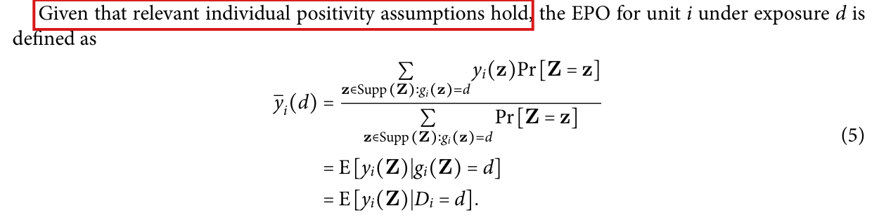
(S5) Exposure probability, positivity, EPO. p. 6, Section 4.1: “we denote the marginal probability that unit $i$ enters exposure $d$ under the design distribution of $\mathbf Z$ as $$\pi_i(d)=\Big(\sum_{\mathbf z\in\mathrm{Supp}(\mathbf Z):g_i(\mathbf z)=d}\Pr[\mathbf Z=\mathbf z]\Big)=\Pr[D_i=d].\qquad(4)$$” “Condition 4.1 (Individual positivity). An exposure $d$ satisfies individual positivity if there exists a $c$ such that $0<c\le\pi_i(d)\ \forall i\in\{1,\ldots,N\}$.” “Given that relevant individual positivity assumptions hold, the EPO for unit $i$ under exposure $d$ is defined as $$\overline y_i(d)=\frac{\sum_{\mathbf z\in\mathrm{Supp}(\mathbf Z):g_i(\mathbf z)=d}y_i(\mathbf z)\Pr[\mathbf Z=\mathbf z]}{\sum_{\mathbf z\in\mathrm{Supp}(\mathbf Z):g_i(\mathbf z)=d}\Pr[\mathbf Z=\mathbf z]}=\mathrm E[y_i(\mathbf Z)|g_i(\mathbf Z)=d]=\mathrm E[y_i(\mathbf Z)|D_i=d].\qquad(5)$$” “To avoid notational overload, these definitions implicitly hold fixed the exposure mapping $g$ and design $\mathbf Z$.” Where two designs are compared the paper writes $\tau_{\mathbf Z}$, $\tau_{\mathbf Z'}$ (Tables 4 and 5, Section 6.3).
(S6) AEPO, EED, AEED. p. 7: “Under individual positivity (Condition 4.1) for exposure $d$ and all individuals $i\in\{1,\ldots,N\}$, we average the EPOs over the units in the population to define the AEPO as $$\overline y(d)=\frac1N\sum_{i=1}^N\overline y_i(d)=\frac1N\sum_{i=1}^N\mathrm E[y_i(\mathbf Z)|D_i=d].\qquad(6)$$” “For an individual observation $i$, assuming that Condition 4.1 holds for exposures $d$ and $d'$ for all individuals $i\in\{1,\ldots,N\}$, we can define the EED between $d$ and $d'$ as $$\tau_i(d,d')=\overline y_i(d)-\overline y_i(d').\qquad(7)$$” “The AEED between $d$ and $d'$ is $$\tau(d,d')=\overline y(d)-\overline y(d')=\frac1N\sum_{i=1}^N\tau_i(d,d').\qquad(8)$$” Footnote 8 (p. 7): “We compare this to the assignment-conditional unit-level treatment effect defined in Sävje, Aronow, and Hudgens (2021): $\tau_i^{AC}(d,d',\mathbf z_{-i})=y_i(d;\mathbf z_{-i})-y_i(d';\mathbf z_{-i})$. In the assignment-conditional unit-level treatment effect, we hold constant treatments assigned to all other individuals at $\mathbf z_{-i}$.”
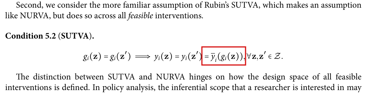
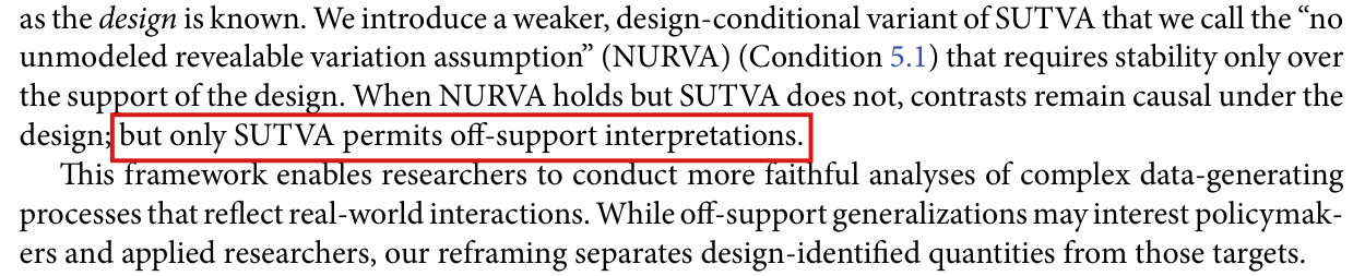
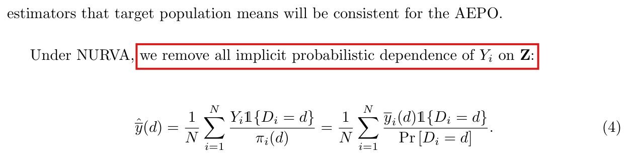
(S7) Stability conditions. p. 8, Section 5.1: “Condition 5.1 (NURVA). $$g_i(\mathbf z)=g_i(\mathbf z')\implies y_i(\mathbf z)=y_i(\mathbf z')=\overline y_i(g_i(\mathbf z)),\ \forall\mathbf z,\mathbf z'\in\mathrm{Supp}(\mathbf Z).$$” “Condition 5.2 (SUTVA). $$g_i(\mathbf z)=g_i(\mathbf z')\implies y_i(\mathbf z)=y_i(\mathbf z')=\overline y_i(g_i(\mathbf z)),\ \forall\mathbf z,\mathbf z'\in\mathcal Z.$$”
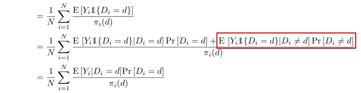
(S8) Estimator. Supplement p. 1: “Throughout, we will require the individual positivity, Condition 4.1, referenced in Section 4.” “We use the Horvitz-Thompson inverse probability weighted estimator (Horvitz and Thompson 1952), as defined in Equation 1, $$\hat{\overline y}(d)=\frac1N\sum_{i=1}^N\frac{Y_i\mathbb 1\{D_i=d\}}{\pi_i(d)}.\qquad(1)$$” Supplement p. 4: “For the AEED, define $\hat\tau(d,d')=\hat{\overline y}(d)-\hat{\overline y}(d')$ and $\pi_{ij}(d,d')=\Pr[D_i=d,D_j=d']$.” Supplement p. 3: “Let the joint exposure probability, $\pi_{ij}(d)=\Pr[D_i=D_j=d]$.”
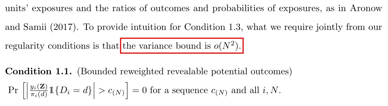
(S9) Asymptotic regime. Supplement p. 5: “We define a sequence of finite populations $U_{(N)}$ indexed by population size $N$. Associated with each finite population $U_{(N)}$ is a known random design vector $\mathbf Z_{(N)}$, a feasible intervention set $\mathcal Z_{(N)}$, $N$ exposure mappings $g_{i,(N)}:\mathcal Z_{(N)}\to\mathbb R$, and $N\times|\mathcal Z_{(N)}|$ raw potential outcomes. Assume that the range of $g_{i,(N)}|\mathrm{Supp}(\mathbf Z_{(N)})$ contains $d$, for all $i,N$. The observed data is $(\mathbf Z_{(N)},\mathbf Y_{(N)})$. We let $N$ tend to infinity.” Note 2 (supplement p. 10): “In the asymptotic regime we could also index observations of, e.g., $y_i$ and $\pi_i(d)$ by $(N)$ but we leave this indexing implicit below.”
(S10) What the paper does not state, and how it is read here. (a) $\mathrm{Supp}(\mathbf Z)$ is not defined; it is read as $\{\mathbf z\in\mathcal Z:\Pr[\mathbf Z=\mathbf z]>0\}$. (b) ‘Finite population’ restricts $N$, not the number of assignments: by (S1) the support is countable, and nothing makes it finite. Every design in the paper's examples and tables has finite support; the general setup admits a countably infinite support with unbounded outcomes (finding P061-CAND-001). (c) No integrability condition is stated anywhere. (d) Conditions 5.1 and 5.2 print no quantifier over $i$; they are read as holding for every $i\in\{1,\ldots,N\}$. Their last equality, $=\overline y_i(g_i(\mathbf z))$, involves an EPO that Equation (5) defines only when $\pi_i(g_i(\mathbf z))>0$: under Condition 5.1 this is automatic and the equality follows from the first one; under Condition 5.2 it is read as holding wherever the EPO is defined (finding P061-CAND-003, a clarity note, whose repair deletes that equality from Condition 5.2). (e) The notation $y_i(d;\mathbf z_{-i})$ of footnote 8 is not defined further; it is read as the raw potential outcome at the assignment vector whose $i$th coordinate is $d$ and whose other coordinates are $\mathbf z_{-i}$, which presupposes that the labels $d,d'$ are assignment coordinates and that the hybrid vector lies in $\mathcal Z$. (f) All probabilities, expectations, variances and covariances are over the design distribution of $\mathbf Z$, with the raw potential outcomes fixed.
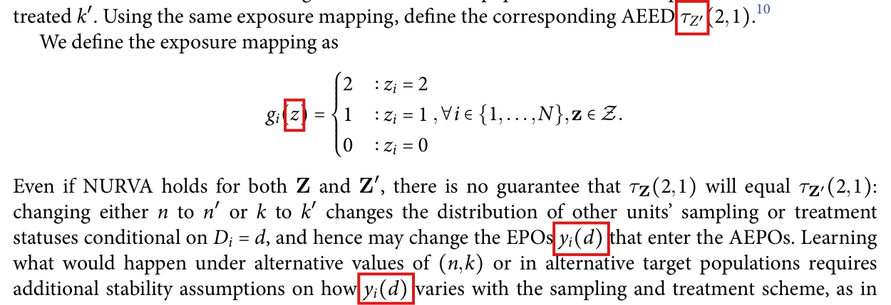
Effective claim (source TeX): As printed. p. 11: ‘Table 4 constructs two schedules of raw potential outcomes. In both cases, the AEED from the observed design, where $\mathrm{Supp}(\mathbf Z)=\{(1,0),(0,1)\}$, does not reflect the AEED in which treatment is delivered uniformly over the population, where $\mathrm{Supp}(\mathbf Z')=\{(1,1),(0,0)\}$.’ ‘When SUTVA is violated, even if NURVA holds, design-specific AEEDs need not generalize to other designs. To illustrate this, consider an experiment where the design space is $\mathcal Z\subseteq\{0,1,2\}^N$, and the exposure mapping is $g_i(\mathbf z)=\begin{cases}1&:z_i>0\\0&:\text{otherwise}\end{cases},\ \forall i\in\{1,\ldots,N\},\mathbf z\in\{0,1,2\}^N$.’ p. 12: ‘For this example, assume that there is no interference in the sense that $y_i(\mathbf z)=y_i(\mathbf z')$ if $z_i=z_i'$.’ ‘If treatments 1 and 2 are associated with different potential outcomes, then the AEED could vary between designs that do and do not sample treatment 2, as in Table 5. (For simplicity, Table 5 displays only assignments in $\mathrm{Supp}(\mathbf Z)$ and $\mathrm{Supp}(\mathbf Z')$; all other feasible assignments have probability zero under the respective designs.)’
Table 4 as printed, rows $(\mathbf z,\ \mathbf d,\ y_1(\mathbf z),\ y_2(\mathbf z),\ \Pr[\mathbf Z=\mathbf z],\ \Pr[\mathbf Z'=\mathbf z])$. (a) Attenuation under uniform rollout: $((0,0),(0,0),0.5,0.5,0,0.5)$, $((0,1),(0,1),0,1,0.5,0)$, $((1,0),(1,0),1,0,0.5,0)$, $((1,1),(1,1),0.5,0.5,0,0.5)$, with ‘$\longrightarrow\tau_{\mathbf Z}(1,0)=1$’ and ‘$\longrightarrow\tau_{\mathbf Z'}(1,0)=0$’. (b) Amplification under uniform rollout: $((0,0),(0,0),0,0,0,0.5)$, $((0,1),(0,1),0,0,0.5,0)$, $((1,0),(1,0),0,0,0.5,0)$, $((1,1),(1,1),1,1,0,0.5)$, with ‘$\longrightarrow\tau_{\mathbf Z}(1,0)=0$’ and ‘$\longrightarrow\tau_{\mathbf Z'}(1,0)=1$’.
Table 5 as printed, rows $(\mathbf z,\ \mathbf d,\ y_1(\mathbf z),\ y_2(\mathbf z),\ \text{probability})$. (a) Design $\mathbf Z$: assigns only in $\{0,1\}$: $((0,1),(0,1),0,1,0.5)$, $((1,0),(1,0),1,0,0.5)$, with ‘$\longrightarrow\tau_{\mathbf Z}(1,0)=1$’. (b) Design $\mathbf Z'$: assigns only in $\{0,2\}$: $((0,2),(0,1),0,2,0.5)$, $((2,0),(1,0),2,0,0.5)$, with ‘$\longrightarrow\tau_{\mathbf Z'}(1,0)=2$’.
Formal content. Table 4: $N=2$, $\mathcal Z=\{0,1\}^2$, $g_i(\mathbf z)=z_i$, $\mathbf Z$ uniform on $\{(0,1),(1,0)\}$ and $\mathbf Z'$ uniform on $\{(0,0),(1,1)\}$. With the raw potential outcomes of panel (a): $\tau_{\mathbf Z}(1,0)=1$ and $\tau_{\mathbf Z'}(1,0)=0$; with those of panel (b): $\tau_{\mathbf Z}(1,0)=0$ and $\tau_{\mathbf Z'}(1,0)=1$; in both panels Condition 5.1 holds under $\mathbf Z$ and under $\mathbf Z'$, and Condition 5.2 fails on $\mathcal Z$. Table 5: $N=2$, $\mathcal Z=\{0,1,2\}^2$, $g_i(\mathbf z)=\mathbb 1\{z_i>0\}$, $y_i(\mathbf z)=z_i$ (the schedule without interference that agrees with the printed rows), $\mathbf Z$ uniform on $\{(0,1),(1,0)\}$ and $\mathbf Z'$ uniform on $\{(0,2),(2,0)\}$: $\tau_{\mathbf Z}(1,0)=1$ and $\tau_{\mathbf Z'}(1,0)=2$; Condition 5.1 holds under $\mathbf Z$ and under $\mathbf Z'$, and Condition 5.2 fails on $\mathcal Z$.
: SAP.P061b.T15Statement
Theorem: SAP.P061b.T15
Statement hash: 91301d59cb005af0fc74a4faa8f8d29b878cf8346e73660d47064ed9d021ddec
Statement definition: SAP.P061b.T15Statement
Certificate. 20261104T182137Z
Declaration review: faithful; 2026-11-04T18:34:16Z; binding v2
Evidence scope: Certification checks formal proof objects. Statement fidelity is a model judgment. Author review is separate.
Proof dependencies: Independently extracted
Source and evidence metadata · sap-2026-11-08-assured-release
















My comment and the history of this entry
My position My comment above.
The models’ position On the available preprint of the linked article, its local-dependence conditions do not ensure that the comparison is defined for general exposure mappings, or that AEED equals an ordinary assignment direct effect, and exact counterexamples persist under them, so a citation alone does not repair the sentence. The closing comparison can materially mislead readers who apply it: Moderate. The published journal version was not checked, and no error in the linked article’s theorem is alleged.