LLM-generated corrections to the published research of P. M. Aronow

Journal article P002

Corrections to: Randomization-based confidence sets for the local average treatment effect

P. M. Aronow, Haoge Chang, and Patrick Lopatto (2026). Randomization-based confidence sets for the local average treatment effect. Biometrika 113(2):asag010.

DOI
10.1093/biomet/asag010
arXiv
2404.18786
Audited edition
Biometrika, 2026, 113(2):asag010; 23 pages in the audited file
SHA-256 of the audited file
825bec9f474745f834453008c778323437d6865e4a449145d0669e5ade435c3a
Permanent address
https://pmaronow.github.io/llm-audit/works/P002/

Summary

The paper constructs confidence sets for the local average treatment effect by inverting a studentized Anderson–Rubin randomization test. Its results are finite-sample validity under a constant additive effect, asymptotic validity under heterogeneous effects with an arbitrarily weak instrument, and algorithms that compute the sets without a grid. 32 entries are classified as errors (2 Moderate, 30 Minor), and 3 are clarity notes. The most consequential is in the code of the replication files, where the fast algorithm can return a bounded set when the set (14) is unbounded (P002-N002). None shows coverage below 1−α1-\alpha for the sets (7) and (11).

What was and was not checked

I checked the following points, which held up. This list is not a statement that the paper is correct, and the absence of a correction elsewhere is not a finding of correctness.

  • The finite-sample argument. Under a constant additive effect, Yi−βDiY_i-\beta D_i does not depend on the assignment at the true β\beta, and the non-strict inversion gives coverage at least 1−α1-\alpha for the sets (7) and (11). I derived this argument and computed coverage by enumeration for n=8,9,10n=8,9,10.
  • The identity for τ^(β)\hat\tau(\beta) on p. 5, the expectation in Supplement Lemma 3, Remarks 1, 2 and 4 (with Supplement Section I), the coefficients (15)–(16) of the AR function, the variance representation (B.1)–(B.2), and the adjusted expansions (F.1)–(F.4), by algebra and against direct numerical evaluation.
  • The steps written out in Supplement Sections C–E, other than those corrected in this audit. I derived each step again. With the corrections, among them P002-E002, the argument written out supports coverage of at least 1−α1-\alpha; the steps that the Supplement omits are listed below.
  • Lemma 1 and Theorem 3 for the algorithms as Step 4 defines them. An independent implementation of Algorithm 2 returns the same sets as direct inversion on a grid for the Bridgeport and Columbus data.
  • Table 1. The coverage of the randomization sets and of 2SLS was simulated again for all seven designs (2000 replications, 1000 simulated assignments) and agrees within Monte Carlo error. Reduced runs based on the research code, for the coverage and median length of the randomization sets, of 2SLS and of the AR sets, agree within Monte Carlo error. The reduced timing benchmark establishes only that Algorithm 4 is faster than Algorithm 3; I did not reproduce the numerical times or the under-one-hour claim at 10410^4 draws.
  • Table 2. The printed compliance rates equal 46/10846/108, 77/10077/100 and 43/6843/68. I compared the six 2SLS intervals and the AR pp-value with the cached output in the replication files; they agree to rounding. Without the STAR data I could not independently verify the compliance rates or rerun the application.
  • Supplement Tables 6–7 for Bridgeport and Columbus. From the provided data I recalculated sample sizes, compliance rates, first-stage FF statistics, point estimates and 2SLS intervals to the displayed rounding. I did not recompute the randomization sets. In Supplement Tables 8–9, the mean sample sizes recompute to the printed precision and the compliance rates are compatible with the subsampling design (P002-N014).
  • The corrected Theorem 2, the corrected Theorem 7 and all four parts of the corrected Lemma 20 are proved in Lean. The precise scope and the additional positive-residual-variance condition for Lemma 20 are described in P002-T5, P002-T21 and P002-T7.

Not checked: Lemma 8, which rests on a cited result; the statements taken from cited works; the tF rows of Table 1, which could not be run; the computation times of Table 1, for which a reduced benchmark confirmed only that Algorithm 4 is faster than Algorithm 3; and Supplement Tables 10–12.

Missing from the replication files: the Project STAR data and the get-out-the-vote data for the four cities other than Bridgeport and Columbus. Without them, the randomization sets of Table 2 and the entries for those four cities in Supplement Tables 6–7 could not be recomputed. The six randomization sets in the cached output for Table 2 differ from the printed ones, by at most about 0.1140.114 at an endpoint, and both versions of the set for SFSP and second-year GPA contain zero. Also missing are the seeds and the saved cases behind Tables 1, 3–5 and 8–10, and the cached output for the get-out-the-vote application is empty. The two binary files of critical values required by the code were unavailable.

Headline claims and related corrections

  1. With the studentized Anderson-Rubin statistic, the randomization-based confidence set (7), and its regression-adjusted version (11), is finite-sample exact under a constant additive treatment effect, and in particular under the sharp null of no effect.

    No numbered result: the opening of Sections 3.3 and 4.4 (citing Imbens & Rosenbaum 2005), equations (3)-(7) and (11); Supplement Lemma 3

    See P002-E001.

  2. Without covariates the same confidence set is asymptotically valid for the LATE under heterogeneous effects, uniformly over a parameter space that allows an arbitrarily weak instrument (bounded standardised fourth moments, a complier covariance condition, treatment fractions bounded away from 0 and 1); the limiting infimum of coverage is exactly 1−α1-\alpha.

    Theorem 1; Assumptions 1-4; Remark 3; Supplement Sections B-C (Lemmas 2-13, Theorems 4-6)

    See P002-E001, P002-E002, P002-E004, P002-E005, P002-E006, P002-E014.

  3. The regression-adjusted confidence set (interacted OLS adjustment) has the same finite-sample and uniform asymptotic guarantees under moment and eigenvalue conditions on the covariates; the adjusted Wald estimator equals the coefficient of the corresponding interacted IV regression.

    Theorem 2; Assumption 5; Remark 4; Supplement Sections D-E (Lemmas 14-20, Theorem 7) and I

    See P002-E001, P002-E002, P002-E003, P002-E007, P002-E008, P002-E009, P002-E010, P002-E013, P002-E014, P002-N009.

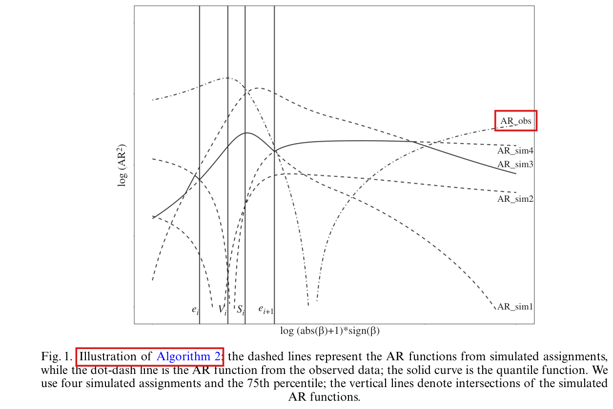
  4. New algorithms recover the Monte Carlo confidence set exactly over the whole real line, without a grid: the index of the simulated AR function that attains the quantile changes only at intersections of two AR functions, which are roots of quartics, and Algorithm 2 skips intersections that do not involve the current quantile function; the same computation serves the regression-adjusted statistic.

    Lemma 1; Theorem 3; Algorithms 1-2 (main text) and 3-4 (Supplement G); Figure 1; Supplement Sections F-H

    See P002-E011, P002-E012, P002-E014, P002-E015, P002-E016, P002-E020, P002-N002, P002-N015, P002-N016, P002-N019, P002-N022.

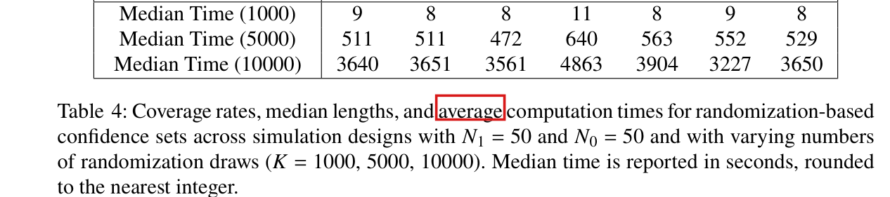
  5. Algorithm 4, the covariate version of Algorithm 2, is much faster than Algorithm 3: with 10410^4 draws it finishes in under an hour where Algorithm 3 takes hours, and with 10310^3 draws both are quick, which makes calculations with 10410^4 draws feasible.

    Section 5.3; Section 6 (p. 19); Table 1, rows 9-12; Supplement Tables 4-5, 'Median Time' rows

    See P002-N002, P002-N003, P002-N011, P002-N012, P002-N018.

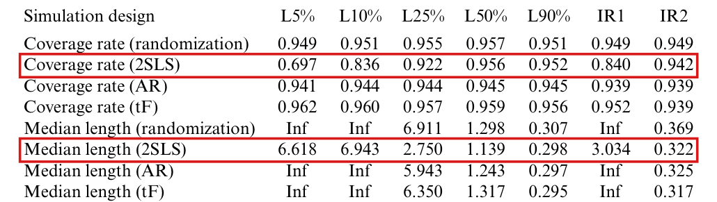
  6. In simulations with n=100n=100 the randomization sets have coverage close to 95% in all seven designs, 2SLS intervals under-cover badly when compliance is low (0.70 at 5% compliance), and the normal-approximation AR and tF sets under-cover in some designs; results do not change materially between 10310^3, 5×1035\times10^3 and 10410^4 draws.

    Section 6; Table 1; Supplement Tables 3-5

    See P002-E018, P002-E019, P002-N012, P002-N013, P002-N018.

  7. For the male subgroup of Project STAR the randomization sets broadly agree with the 2SLS intervals, except that for SFSP and second-year GPA the 2SLS interval excludes zero (and the normal-approximation AR test gives p=0.04p=0.04) while the randomization set includes zero, despite a high reported first-stage FF.

    Section 7; Table 2

  8. In the six get-out-the-vote experiments the randomization sets are close to the 2SLS intervals and adjusting for prior turnout shortens them; when the Bridgeport sample is subsampled to smaller size and lower compliance the randomization sets become longer relative to 2SLS, 2SLS coverage departs from nominal, and the randomization sets keep nominal coverage.

    Section 7 (pointer on p. 20); Supplement Sections K-L; Supplement Tables 6-12

    See P002-E017, P002-N014, P002-N015.

Corrections

Moderate (2)

A real substantive error with limited reach.

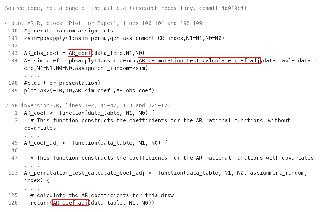
When the intersection reached by the loop of Algorithm 2 is the largest of all intersections, both implementations in the replication code keep the previous quantile index for the final interval instead of choosing mi+1∈I(ei+1)m_{i+1}\in\mathcal I(e_i+1); the returned set can then differ from (14) to the right of the last intersection and can be bounded where (14) is unbounded.

Algorithm 2, Step 4, p. 16 (the same step in Algorithm 4, Supplementary Material p. 44), as implemented in the replication code: research code, 2_AR_inversion_algo2.R, lines 287–292 (and 103–108); rilate package, R/AR_algo2.R, lines 178–180

As printed

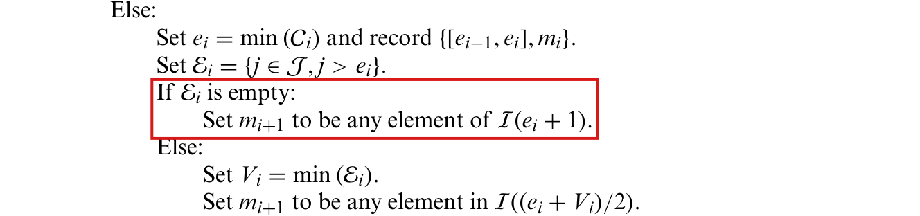
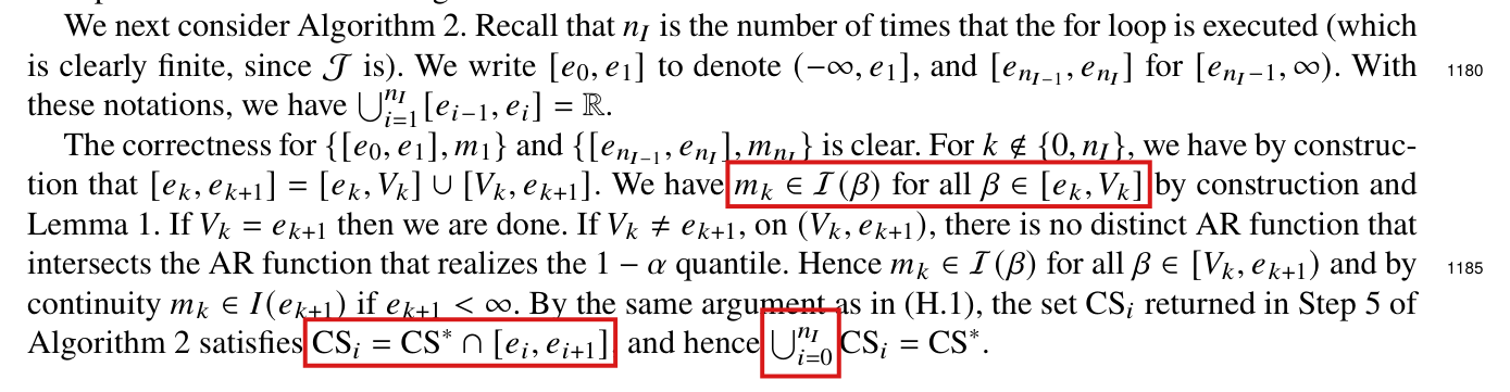
Algorithm 2, Step 4, p. 16: “Set ei=min⁡(Ci)e_i=\min(\mathcal C_i) and record {[ei−1,ei],mi}\{[e_{i-1},e_i],m_i\}. Set Ei={j∈J,j>ei}\mathcal E_i=\{j\in\mathcal J,j>e_i\}. If Ei\mathcal E_i is empty: Set mi+1m_{i+1} to be any element of I(ei+1)\mathcal I(e_i+1).”

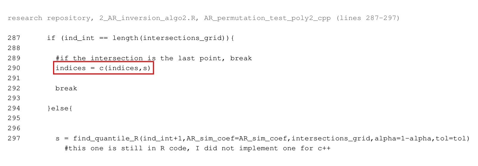
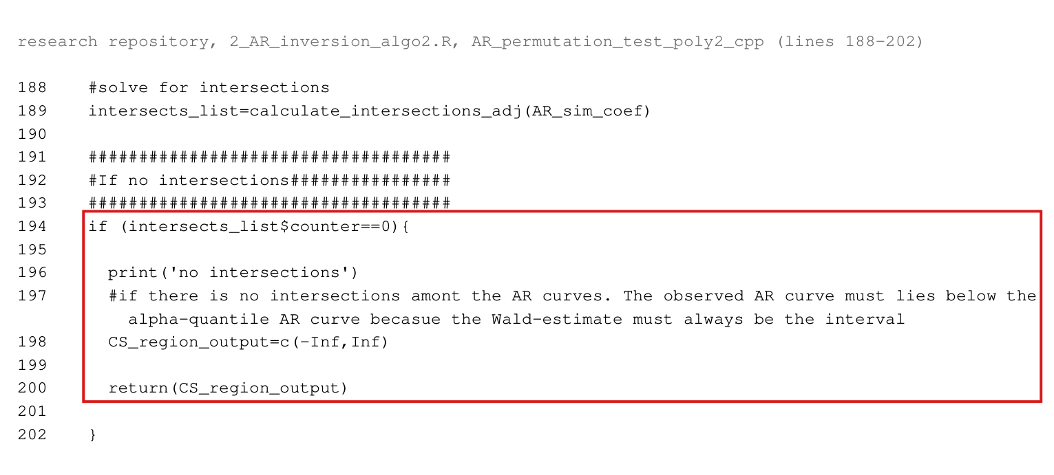
Research code, 2_AR_inversion_algo2.R, lines 287, 290 and 292, where s is the current quantile index:

if (ind_int == length(intersections_grid)){

indices = c(indices,s)

break

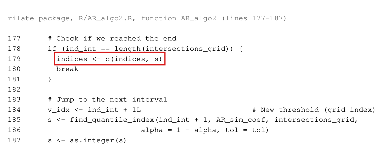
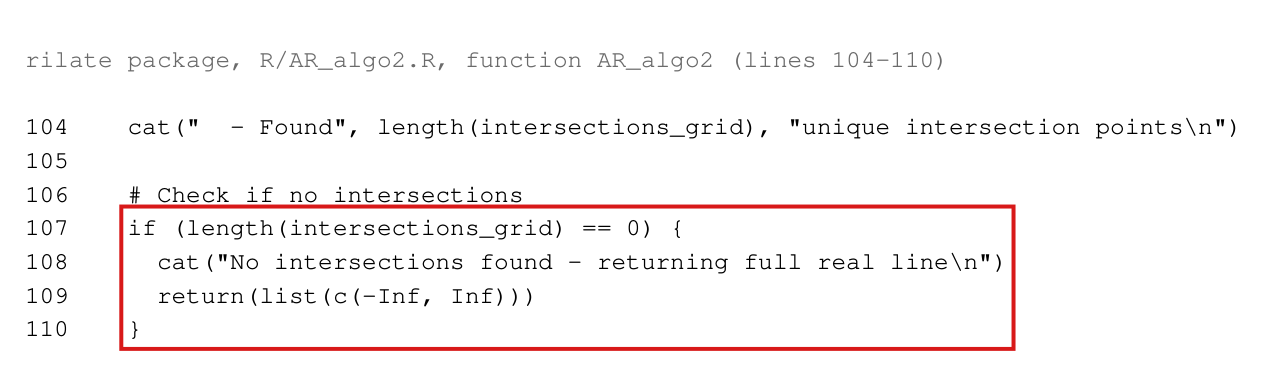
The rilate package, R/AR_algo2.R, lines 178–180:

if (ind_int == length(intersections_grid)) {

indices <- c(indices, s)

break

The problem

Step 4 follows the simulated AR function that currently realizes the quantile, with index mim_i, to its next intersection eie_i, and then chooses a new index for the interval to the right of eie_i. The printed step does this in both cases: when later intersections exist it evaluates I\mathcal I between eie_i and the next one, and when eie_i is the largest of all intersections it evaluates I\mathcal I at ei+1e_i+1. The code carries out the first case. In the second case it appends the current index s, which is mim_i, for the final interval and leaves the loop. If the crossing changes the function that realizes the quantile, the code compares the observed AR function with the wrong simulated one on (ei,∞)(e_i,\infty). The returned set then differs from the intended inversion where the observed function is strictly above the smaller of the two critical functions and at or below the larger. The difference between the two sets consists either only of added points or only of deleted points, and it can be unbounded.

The defect is confined to the interval to the right of the largest intersection of simulated AR functions. Its effect on the reported numbers is not known. When the last intersection is a unique simple crossing of two singly occurring functions, the kept function is one rank away from the correct one, but this bounds neither how often the branch is reached nor how far an endpoint moves: in the example below the kept function is exactly one rank away at M=1000M=1000, 50005000 and 10410^4, and the right endpoint moves from ∞\infty to 1212.

Evidence an exact counterexample

The evidence is an exact counterexample, run through the unmodified code of both sources, and a derivation. I take eight units, four of them treated in every assignment, with the observed assignment ZZ and four other assignments AA, BB, HH and LL:

Data of the example: outcome, treatment received, the observed assignment and four assignments used for the simulation.
YYDDZZAABBHHLL
33111111111111
33001111000000
−1-1111100111111
−1-1111100001100
11110011111100
11000011000011
−3-3000000110011
−3-3000000000000

For an assignment jj let tj(β)t_j(\beta) be the difference of the arm means of Y−βDY-\beta D, and let T(β)=2(β−1)2+38T(\beta)=2(\beta-1)^2+38. The squared AR function of jj is Fj=16tj2/(T−2tj2)F_j=16t_j^2/(T-2t_j^2), with positive denominator, and

tZ=2−β2,tA=4,tB=−β2,tH=1−β,tL=0.t_Z=2-\tfrac\beta2,\qquad t_A=4,\qquad t_B=-\tfrac\beta2,\qquad t_H=1-\beta,\qquad t_L=0 .

Since FjF_j is increasing in tj2t_j^2, every comparison reduces to one between squares of these linear functions. The simulated AR functions intersect at −8,−3,0,2/3,1,2,5-8,-3,0,2/3,1,2,5 and 88, and the largest intersection, at β=8\beta=8, is a crossing of FAF_A and FBF_B. Further,

FZ≤FA  ⟺  −4≤β≤12,FZ≤FB  ⟺  β≥2,FZ≤FH  ⟺  ∣β∣≥2.F_Z\le F_A\iff-4\le\beta\le12,\qquad F_Z\le F_B\iff\beta\ge2,\qquad F_Z\le F_H\iff|\beta|\ge2 .

Let rr be the rank of the quantile, and let the MM simulated assignments be r−2r-2 copies of LL, one copy each of AA and BB, and M−rM-r copies of HH. The squared critical value at rank rr is then min⁡{FH,max⁡(FA,FB)}\min\{F_H,\max(F_A,F_B)\}, and max⁡(FA,FB)\max(F_A,F_B) equals FAF_A for ∣β∣≤8|\beta|\le8 and FBF_B otherwise. For (13), r=⌈0.95M⌉r=\lceil0.95M\rceil, and I obtain

I^0.95∗(Z)=[−4,−2]∪[2,∞).\widehat I^*_{0.95}(Z)=[-4,-2]\cup[2,\infty).

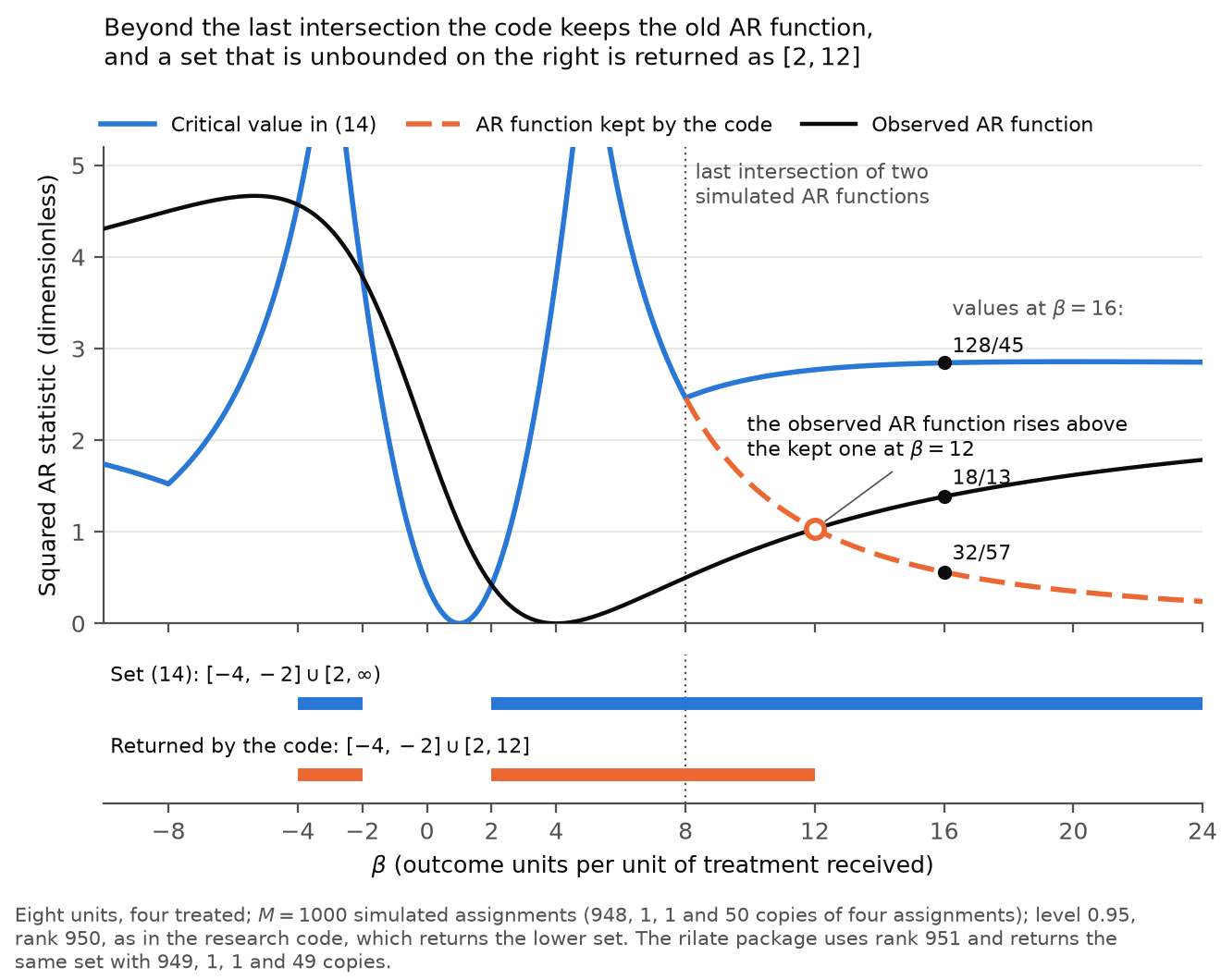
Just left of β=8\beta=8 the quantile is realized by AA, and just right of it by BB. The code keeps AA on (8,∞)(8,\infty) and returns [−4,−2]∪[2,12][-4,-2]\cup[2,12]. At β=16\beta=16 the kept function equals 32/5732/57, the observed function 18/1318/13 and the squared critical value 128/45128/45.

Sets returned at M=1000M=1000 and confidence level 0.950.95. The last column is the intended inversion at each routine’s own rank; (13) uses rank 950950, while the package uses 951951.
RoutineRank rrReturnedAfter the repair below
Research code (C++ path), no covariate950950[−4,−2]∪[2,12][-4,-2]\cup[2,12][−4,−2]∪[2,∞)[-4,-2]\cup[2,\infty)
rilate, no covariate951951[−4,−2]∪[2,12][-4,-2]\cup[2,12][−4,−2]∪[2,∞)[-4,-2]\cup[2,\infty)
Research code (C++ path), one covariate950950[−20,−18]∪[−14,−4][-20,-18]\cup[-14,-4][−20,−18]∪[−14,∞)[-20,-18]\cup[-14,\infty)
rilate, one covariate951951[−20,−18]∪[−14,−4][-20,-18]\cup[-14,-4][−20,−18]∪[−14,∞)[-20,-18]\cup[-14,\infty)

The rows with a covariate use 3232 units, obtained by repeating each unit four times, with a covariate taking the values −1,−1,1,1-1,-1,1,1 within each group of four and with YY replaced by Y−16DY-16D. The endpoints in these rows agree with the stated values to 10−1210^{-12}. In these rows the returned set excludes the value 00, which the intended set contains. With the same construction, the stated sets also hold at M=5000M=5000 and M=104M=10^4, with ranks 47504750 and 95009500 for the research code and 47514751 and 95019501 for the package; the code was run at M=1000M=1000 only. A second, independent example with eight simulated assignments has set (−∞,−3]∪[−1,∞)(-\infty,-3]\cup[-1,\infty), and both routines return only (−∞,−3](-\infty,-3].

With correctly computed intersections and quantile indices, the repair is justified as follows. Under Assumption 6, or Assumption 7 with covariates, the squared AR functions are continuous, and two distinct ones differ by a rational function with at most four real zeros. To the right of the largest intersection no difference changes sign, so the order of the simulated values is constant there. Any index in I(ei+1)\mathcal I(e_i+1) realizes the quantile on the whole final interval, including its left endpoint by continuity.

The effect of the defect on the reported numbers is not established. The simulated assignments of the published runs are not in the replication files, and neither are the data of the application to Angrist et al. or of four of the six cities. An argument that the branch is reached with probability of order 2/M2/M does not hold in general: for four units with Y=(0,1,2,4)Y=(0,1,2,4), D=(1,1,0,0)D=(1,1,0,0) and two treated, under complete randomization, the code keeps a wrong index with probability at least 1−2×10−1061-2\times10^{-106} at M=1000M=1000. Coverage over 50005000 data sets moves in steps of 0.00020.0002, and one changed decision can change a printed third decimal.

What survives

Step 4 as printed, Lemma 1, the definitions (13)–(17), Theorem 3 and the theory for the confidence sets are unaffected by this code defect. This defect does not change membership at or to the left of the largest intersection of simulated AR functions. A value β\beta to the right of it changes status only if the observed AR function is strictly above the smaller of the kept function and the correct one and at or below the larger; in particular a changed coverage decision at the true value 00 in Section 6 requires both a negative largest intersection and this bracket at 00. The p-value of the rilate package at β=0\beta=0 is computed separately and is unaffected. The procedures that do not use randomization critical values are unaffected. The simulation and application scripts of the research code call the affected routine. I have not established whether any reported entry changes: this applies to the coverage rates and lengths of the randomization sets in Table 1 and Supplementary Tables 3–5 and 12, to their endpoints in Table 2 and Supplementary Tables 6 and 7, and to the relative lengths in Supplementary Table 10.

Corrected

The printed text needs no change. In the code, the branch for the last intersection should select the index for the final interval before recording it. In the research code:

if (ind_int == length(intersections_grid)){

s = as.integer(find_quantile_R(ind_int+1,AR_sim_coef,intersections_grid,alpha=1-alpha,tol=tol))

indices = c(indices,s)

break

In the rilate package:

if (ind_int == length(intersections_grid)) {

s <- as.integer(find_quantile_index(ind_int + 1L, AR_sim_coef, intersections_grid, alpha = 1 - alpha, tol = tol))

indices <- c(indices, s)

break

The second wrapper of the research code, written in R only (lines 103–108), needs the same line with its fixed significance level 0.050.05. The index already recorded for the preceding interval is kept.

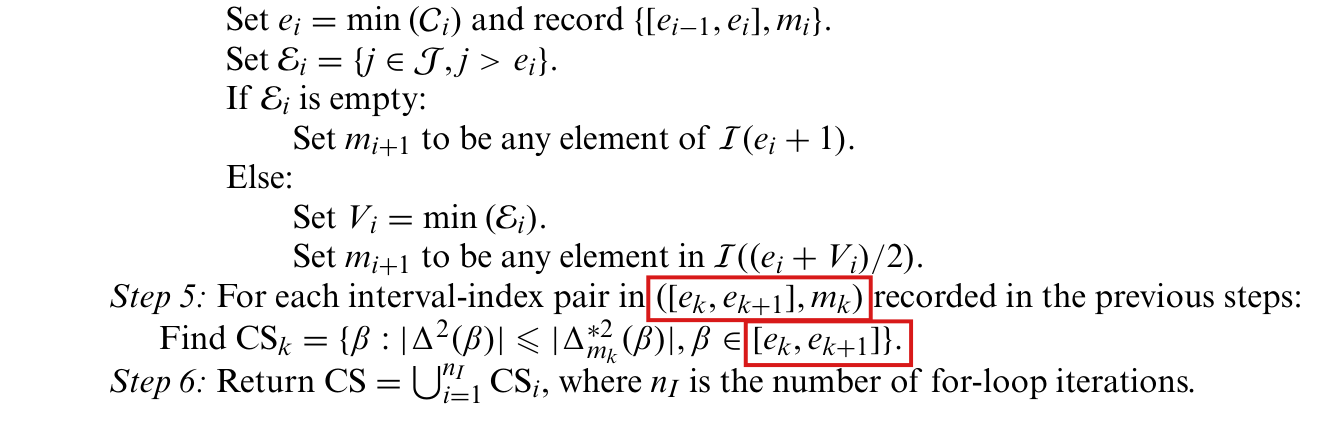
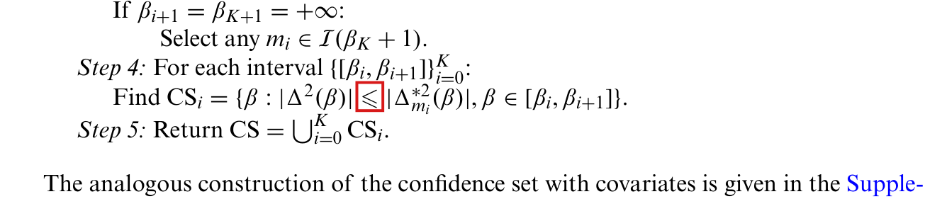
Crop of the second half of Step 4 of Algorithm 2, from 'Else: Set e i equal to min of C i and record' to 'Set m i plus 1 to be any element in I of e i plus V i over 2'. A red box marks the two lines 'If E i is empty: Set m i plus 1 to be any element of I of e i plus 1'.
Algorithm 2, Step 4, p. 16. The marked branch chooses a new index after the last intersection; the code omits this choice.
Listing of lines 287 to 297 of the function AR_permutation_test_poly2_cpp. An if statement tests whether ind_int equals the length of intersections_grid, with the comment 'if the intersection is the last point, break'. A red box marks line 290, 'indices = c(indices,s)', followed by break. In the else branch, line 297 sets s to find_quantile_R of ind_int+1.
Research code, 2_AR_inversion_algo2.R, lines 287–297 (a listing of the replication code, with line numbers added). At the last intersection the marked line records the current index s for the final interval; the call that selects a new index is made only in the other branch, on line 297.
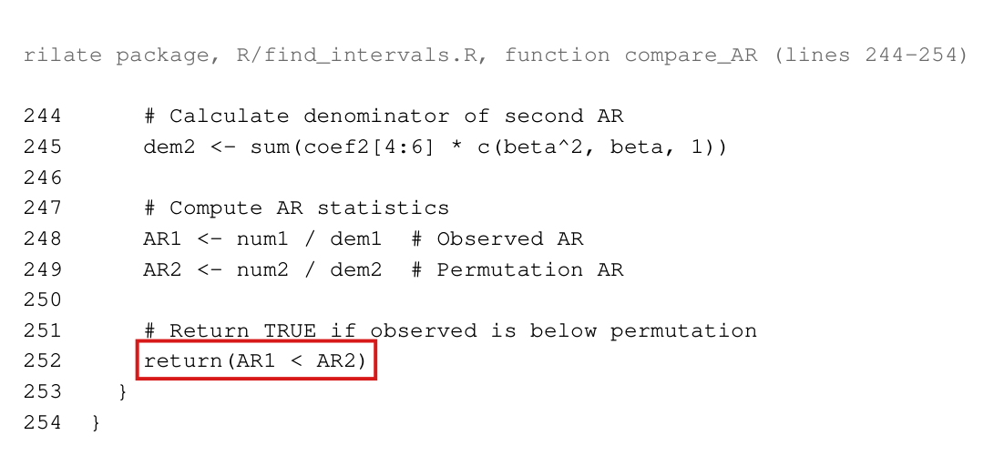
Listing of lines 177 to 187 of the function AR_algo2. Under the comment 'Check if we reached the end', an if statement tests whether ind_int equals the length of intersections_grid. A red box marks line 179, 'indices <- c(indices, s)', followed by break. After the if block, lines 185 to 187 set s to find_quantile_index of ind_int + 1.
The rilate package, R/AR_algo2.R, lines 177–187 (a listing of the replication code, with line numbers added). The marked line records the current index for the final interval.
Line chart with a strip below it. The horizontal axis is beta from minus 10 to 24; the vertical axis is the squared AR statistic from 0 to 5.2. A blue curve, the squared critical value used in (14), has two tall peaks, falls to about 2.5 at beta equal to 8, and then stays near 2.8. A black curve, the observed AR function, falls from about 4.6 near beta equal to minus 5 to zero at beta equal to 4 and rises slowly to about 1.8 at beta equal to 24. A dashed orange curve, the AR function kept by the code, starts at beta equal to 8, where a dotted vertical line marks the last intersection, and falls towards zero; an open circle marks where the black and orange curves meet at beta equal to 12. At beta equal to 16 three dots are labelled 128/45 on the blue curve, 18/13 on the black curve and 32/57 on the orange curve. In the strip, a blue bar shows the set (14), from minus 4 to minus 2 and from 2 to the right edge, and an orange bar shows the returned set, from minus 4 to minus 2 and from 2 to 12.
The eight-unit example at M=1000M=1000. Upper panel: the observed squared AR function, the squared critical value used in (14), and the simulated AR function that the code keeps beyond the last intersection of two simulated AR functions, at β=8\beta=8. Lower panel: the set (14) and the set returned by the code. To the right of β=12\beta=12 the observed function lies above the kept function and below the squared critical value, so the code rejects values that (14) accepts.

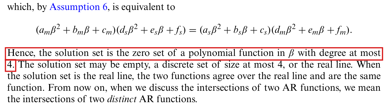
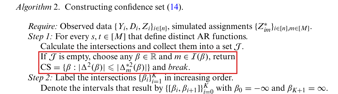
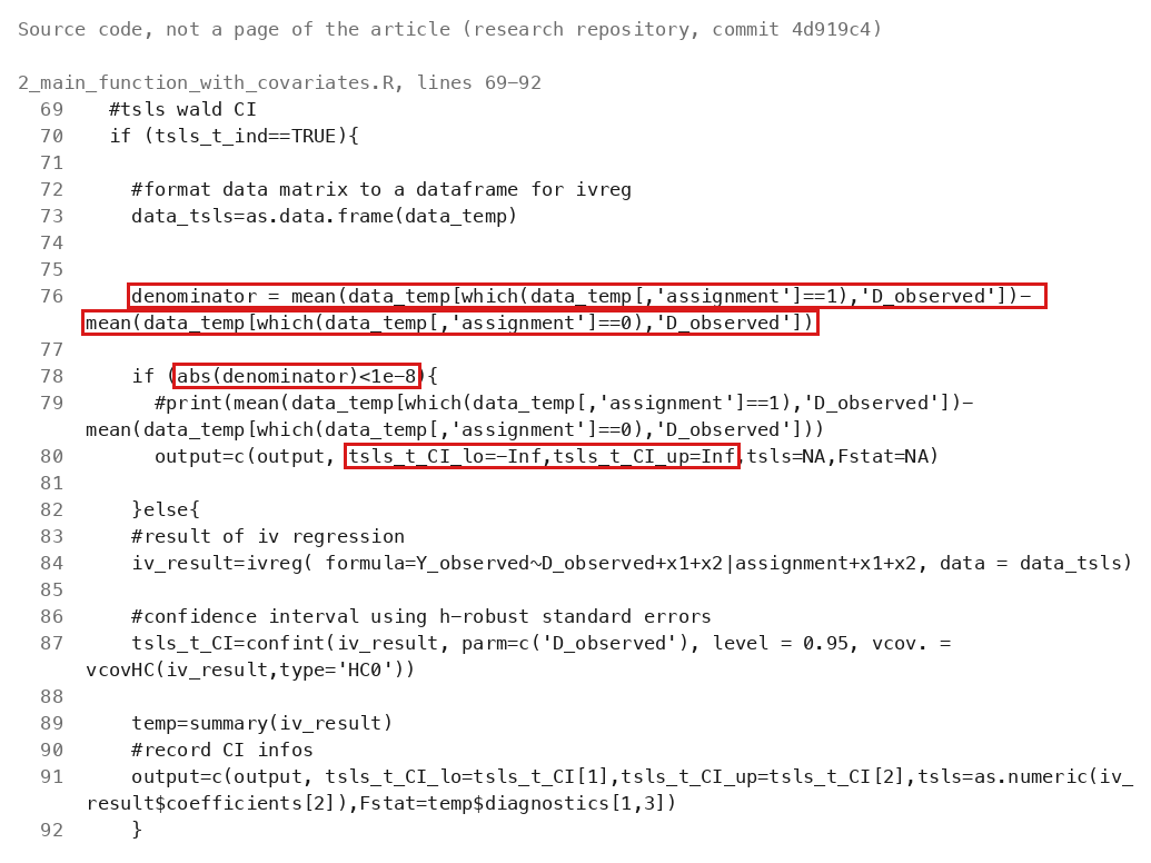
The replication code uses a fixed absolute threshold of 10−810^{-8} to decide the degree and identity of intersection polynomials, and it can then miss intersections of AR functions and treat distinct AR functions as identical; with binary outcome and treatment and a large sample it returns the whole real line where the confidence set (14) is a bounded interval.

Remark 7, p. 14, and Step 1 of Algorithms 1 and 2, pp. 15–16, as implemented in the replication code: rilate package, R/calculate_intersections.R, lines 140–165; research code, AR_intersection in 2_AR_inversion_algo1.R and find_root in cpp_implementations/auxiliary_functions.cpp

As printed

Remark 7, p. 14: “Hence, the solution set is the zero set of a polynomial function in β\beta with degree at most 4. The solution set may be empty, a discrete set of size at most 4, or the real line. When the solution set is the real line, the two functions agree over the real line and are the same function.”

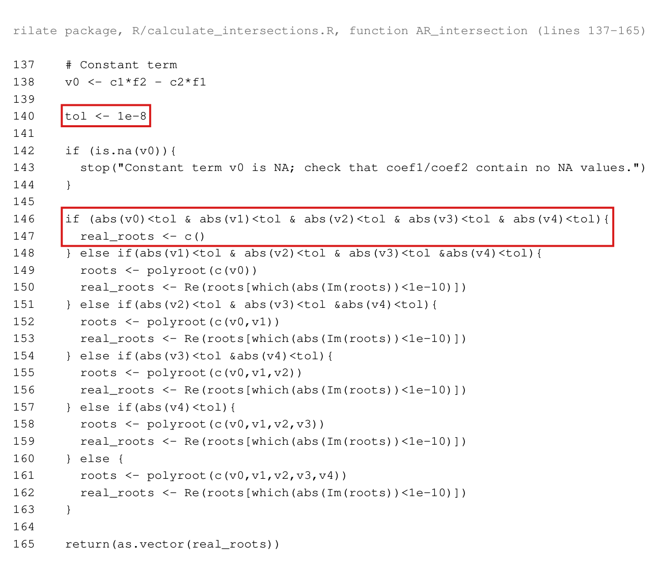
The rilate package, R/calculate_intersections.R, lines 140 and 146–147, where v0, …, v4 are the coefficients of the polynomial:

tol <- 1e-8

if (abs(v0)<tol & abs(v1)<tol & abs(v2)<tol & abs(v3)<tol & abs(v4)<tol){

real_roots <- c()

The branches that follow use the same threshold to choose the degree of the polynomial that is solved. The research code has the same tests with the same threshold.

The problem

Let Δm∗2=Nm/Qm\Delta_m^{*2}=N_m/Q_m be the squared AR function of a simulated assignment mm, where NmN_m and QmQ_m are the quadratics of (16). Under Assumption 6, two such functions meet exactly at the real zeros of Pms=NmQs−NsQm=∑j=04vjβjP_{ms}=N_mQ_s-N_sQ_m=\sum_{j=0}^4v_j\beta^j, and they are the same function exactly when all five coefficients vjv_j are zero. This is Remark 7. The code replaces “vj=0v_j=0” by “∣vj∣<10−8|v_j|<10^{-8}”, both to decide whether two functions are the same and to choose the degree of the polynomial that it solves. The coefficients vjv_j have no fixed scale. Multiplying the coefficient vectors of both functions by t>0t>0 multiplies every vjv_j by t2t^2 and leaves the functions unchanged, and in the binary examples below the vjv_j decrease as nn grows. The code discards nonzero terms that are below the threshold, which can change the set of real zeros. When all five coefficients of a pair are below the threshold, it reports no intersection for that pair. When this happens for every pair, the grid of intersections is empty and the code for Algorithm 2 returns the whole real line (P002-E015).
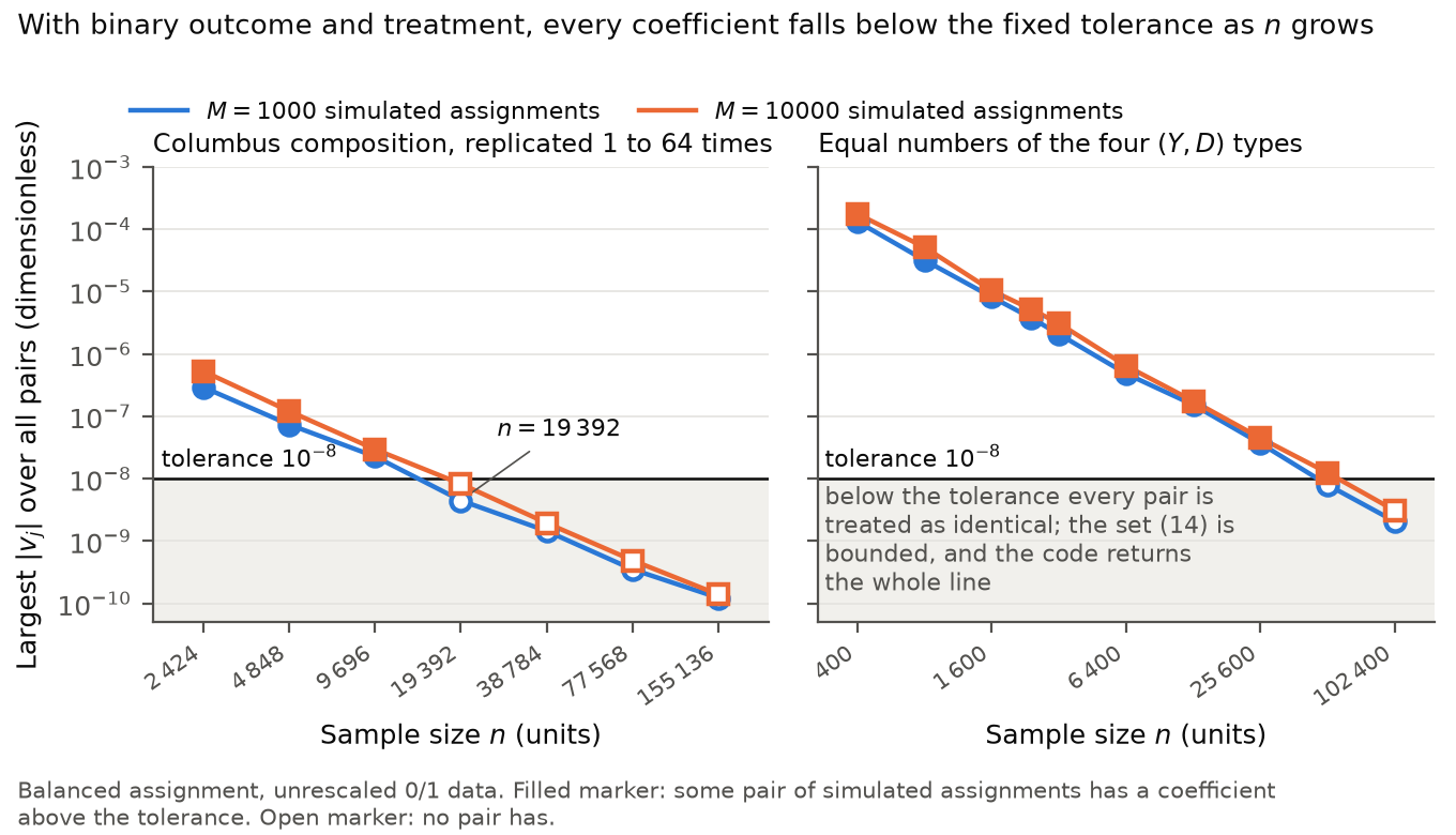
The threshold is reached on unrescaled data in the settings of the paper. In recalculations with the same simulated assignments, nonzero terms were discarded in one saved data set for each of the fourteen combinations of design and allocation of Section 6 (M=1000M=1000) and in the Bridgeport and Columbus data, with and without the covariate. In one recalculation for Columbus without the covariate at M=1000M=1000, 51 70551\,705 pairs of distinct functions are classified as identical and the code reports 621 548621\,548 real roots, compared with 977 137977\,137 for the full polynomials, counted separately for each pair. Every endpoint returned in these runs still agrees with the exact set (14), or (F.4) with the covariate, to three decimals. The largest error is approximately 0.00003360.0000336, at the lower endpoint for Columbus with the covariate at M=104M=10^4, where the code returns approximately −0.041607-0.041607 and the exact value is approximately −0.041574-0.041574. The failure is of a different kind when outcome and treatment are binary and the sample is large: the code returns the whole real line where (14) is a short interval. This occurs from n=1176n=1176 in a constructed family and at n=19 392n=19\,392 for the composition of the Columbus data with independent simulated assignments.

Evidence an exact counterexample

I use exact counterexamples, run through the unmodified R and C++ code, and recalculations using exact zeros and roots of the calculated AR functions.

First, consider the coefficient vectors (1,0,0,1,0,1)(1,0,0,1,0,1) and (1,−2,1,1,0,1)(1,-2,1,1,0,1), which represent β2/(β2+1)\beta^2/(\beta^2+1) and (β−1)2/(β2+1)(\beta-1)^2/(\beta^2+1). Their only intersection is β=1/2\beta=1/2, and P=(2β−1)(β2+1)P=(2\beta-1)(\beta^2+1). After both vectors are multiplied by 10−510^{-5} each function is unchanged, the coefficients of PP are (−10−10,2×10⁻¹⁰,−10−10,2×10−10,0)(-10^{-10},2\times10^{-10},-10^{-10},2\times10^{-10},0), and the root finders of the rilate package and of the research code (R and C++) return no intersection. The interval routine of the package then returns the whole real line where the first function is at most the second exactly on (−∞,1/2](-\infty,1/2].

Second, I take eight units with Y=(0,1,2,3,4,5,6,8)Y=(0,1,2,3,4,5,6,8) and D=Z=(0,0,0,0,1,1,1,1)D=Z=(0,0,0,0,1,1,1,1), and M=40M=40 simulated assignments consisting of 2020 copies each of (1,0,0,0,0,1,1,1)(1,0,0,0,0,1,1,1) and (0,1,0,0,0,1,1,1)(0,1,0,0,0,1,1,1). All denominators are positive, the two simulated AR functions intersect only at β=5\beta=5, and the set (14) at level 0.950.95 is [3,14/3][3,14/3]. The package returns this interval to within 10−1210^{-12}. When the outcomes are multiplied by 10−710^{-7}, the set (14) is [3×10⁻⁷, (14/3)×10−7][3\times10^{-7},\,(14/3)\times10^{-7}], the code loses the intersection at 5×10−75\times10^{-7}, and AR_algo2 returns the whole real line.

Third, no rescaling is needed. Let nn be a multiple of 88 such that n>8n>8, and consider n/4n/4 units of each type (Y,D)∈{(0,0),(1,0),(0,1),(1,1)}(Y,D)\in\{(0,0),(1,0),(0,1),(1,1)\} with n/2n/2 treated. Let the observed treatment group contain 00, n/8n/8, n/8n/8 and n/4n/4 units of these types, the first simulated one n/8−1n/8-1, n/8+1n/8+1, n/8n/8 and n/8n/8, and the second n/8−1n/8-1, n/8n/8, n/8+1n/8+1 and n/8n/8, with 2020 copies of each simulated assignment. In the representation used by the code, the numerators are No=(β−1)2/4N_o=(\beta-1)^2/4, N1=16/n2N_1=16/n^2 and N2=16β2/n2N_2=16\beta^2/n^2, the denominators are Qj=(β2+1−Nj)/n>0Q_j=(\beta^2+1-N_j)/n>0, and

P12(β)=16n3 (1−β4),I^0.95∗(Z)=[1−8n, nn−8].P_{12}(\beta)=\frac{16}{n^3}\,(1-\beta^4),\qquad\widehat I^*_{0.95}(Z)=\Big[1-\frac8n,\ \frac{n}{n-8}\Big].

The two simulated AR functions intersect at ±1\pm1. The code discards P12P_{12} when 16/n3<10−816/n^3<10^{-8}, that is, for n≥1170n\ge1170. At n=1168n=1168 it finds both intersections and returns a bounded set. At n=1176n=1176 the set (14) is [146/147, 147/146][146/147,\,147/146], and the package returns (−∞,∞)(-\infty,\infty).

Fourth, independent simulated assignments lead to the same state. For the pooled composition of the Columbus data (20752075, 190190, 130130 and 2929 units of the four types) replicated 88 times, n=19 392n=19\,392, with balanced assignment and M=1000M=1000 or M=104M=10^4 independent simulated assignments, the largest ∣vj∣|v_j| over all pairs is below 10−810^{-8}, while (14) equals [−14/323, 50/629][-14/323,\,50/629] and [−14/323, 50/621][-14/323,\,50/621] respectively. At n=9696n=9696 some pair is still above the threshold. There is no threshold in nn alone: for equal numbers of the four types the first tested size is 51 20051\,200 at M=1000M=1000 and 102 400102\,400 at M=104M=10^4.

The confidence set (14), or (F.4) with the covariate, and the set returned by the code, for the same data and simulated assignments.
ExampleSet (14) or (F.4)Returned by the code
Eight units, outcomes multiplied by 10−710^{-7}[3×10⁻⁷, (14/3)×10−7][3\times10^{-7},\,(14/3)\times10^{-7}](−∞,∞)(-\infty,\infty)
Binary family, n=1176n=1176, M=40M=40[146/147, 147/146][146/147,\,147/146](−∞,∞)(-\infty,\infty)
Columbus composition, n=19 392n=19\,392, M=1000M=1000[−14/323, 50/629][-14/323,\,50/629](−∞,∞)(-\infty,\infty)
Columbus data with covariate, M=104M=10^4 (rounded)[−0.041574, 0.266049][-0.041574,\,0.266049][−0.041607, 0.266049][-0.041607,\,0.266049]

The first and second rows were run through the unmodified code. The fourth used the same root and inversion decisions with optimized storage and grid searches. In the third row the returned set follows from the classification of all pairs, which was computed exactly. In the fourth row the set is the regression-adjusted analogue (F.4) of (14).

What survives

Remark 7, Lemma 1, Algorithms 1 to 4 as printed and Theorem 3 use the actual intersections and are not contradicted by this code defect. The definitions of the confidence sets and the finite-sample and asymptotic theory are unaffected. No reported value is shown to change: every endpoint checked in the Section 6 and city recalculations agrees with exact inversion at the three decimals printed in Supplementary Tables 6 and 7. The checks do not cover the application to the data of Angrist et al., the cities Raleigh, Minneapolis, Detroit and St. Paul, or the Bridgeport subsamples, whose inputs are not in the replication files, and they do not use the simulated assignments of the published runs. The research code also contains a C++ routine in exact integer arithmetic. It tests for exact zero and is not affected. A user who applies the replication code to a large experiment with binary outcome and treatment can obtain the whole real line where (14) is bounded.

Corrected

The printed text needs no change. In the code, replace the fixed threshold by exact or certified tests of vj=0v_j=0, both for the identity of two AR functions and for the degree of PmsP_{ms}; keep every nonzero coefficient; and compute all real zeros of NmQs−NsQmN_mQ_s-N_sQ_m. The coefficients may be rescaled for the numerical solution, but no term may be dropped. When no pair of simulated AR functions intersects, the code must carry out the comparison of Step 1 of Algorithm 2 (P002-E015).

The set (14) can also be computed without the pairwise intersections. Under Assumption 6, with Pom=NoQm−NmQoP_{om}=N_oQ_m-N_mQ_o and k=⌈(1−α)M⌉k=\lceil(1-\alpha)M\rceil,

β∈I^1−α∗(Z)  ⟺  #{m:Δm∗2(β)<Δ2(β)}≤k−1  ⟺  #{m:Pom(β)≤0}≥M−k+1,\beta\in\widehat I^*_{1-\alpha}(Z)\iff\#\{m:\Delta_m^{*2}(\beta)<\Delta^2(\beta)\}\le k-1\iff\#\{m:P_{om}(\beta)\le0\}\ge M-k+1,

so the set is determined by the signs of the nonzero polynomials PomP_{om} between their real zeros and at those zeros; identically zero polynomials count toward the inequality for every β\beta.

Crop of the second half of Remark 7, from 'which, by Assumption 6, is equivalent to' and the displayed product equation to the end of the remark. Red boxes mark the sentence 'Hence, the solution set is the zero set of a polynomial function in beta with degree at most 4.'
Remark 7, p. 14. The marked sentence is the statement that the code is intended to implement: the intersections are the real zeros of a polynomial of degree at most 4.
Listing of lines 137 to 165 of the function AR_intersection. A red box marks line 140, 'tol <- 1e-8'. A second red box marks lines 146 and 147, an if statement that tests whether the absolute values of v0, v1, v2, v3 and v4 are all below tol and, if so, sets real_roots to an empty vector. The following else-if branches test fewer coefficients against tol and call polyroot on a polynomial of lower degree.
The rilate package, R/calculate_intersections.R, lines 137–165 (a listing of the replication code, with line numbers added). The marked lines fix the threshold and return no intersection when all five coefficients are below it.
Two line charts with logarithmic axes. The horizontal axis is the sample size n and the vertical axis is the largest absolute coefficient over all pairs, labelled from 10 to the minus 10 to 10 to the minus 3. A horizontal black line marks the tolerance 10 to the minus 8, and the region below it is shaded. In each panel a blue line with circles is M equal to 1000 and an orange line with squares is M equal to 10000; both fall steadily as n grows. In the left panel, Columbus composition, the points at n equal to 2424, 4848 and 9696 are filled and above the tolerance, and the points from n equal to 19392 to 155136 are open and below it. In the right panel, equal numbers of the four types, the points are filled up to n equal to 25600; at 51200 the M equal to 1000 point is open and the M equal to 10000 point is filled, and at 102400 both are open.
The largest absolute coefficient of the intersection polynomials, over all pairs of simulated assignments, against the sample size, for two populations with binary outcome and treatment and balanced assignment. Left: the composition of the Columbus data, replicated 11 to 6464 times. Right: equal numbers of the four types (Y,D)(Y,D). Below the horizontal line every pair is classified as identical, the code finds no intersection, and its empty-grid branch returns the whole real line. The exact set (14) is a bounded interval at every point shown.

Minor (30)

Real but inconsequential, for example a misprint that does not change a result.

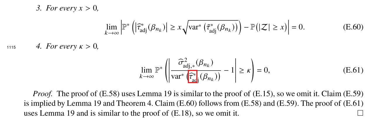
In (E.61) the denominator should be the reassignment variance of the infeasible statistic τ~adj∗\tilde\tau^*_{\mathrm{adj}}, as in (E.58)–(E.60), not that of the feasible statistic τ^adj∗\widehat\tau^*_{\mathrm{adj}}.

Supplement, Lemma 20, item 4, display (E.61), p. 42 (PDF p. 22 of the Supplement)

See also under Formal statements (Lean): P002-T6, P002-T7

As printed

4. For every κ>0\kappa>0,

lim⁡k→∞P∗(∣σ^adj,∗2(βnk)var⁡∗(τ^adj∗(βnk))−1∣≥κ)=0,(E.61)\lim_{k\to\infty}\mathbb P^*\left(\left|\frac{\widehat\sigma^2_{\mathrm{adj},*}(\beta_{n_k})}{\operatorname{var}^*\big(\colorbox{#ffe58a}{$\displaystyle \widehat\tau$}^*_{\mathrm{adj}}(\beta_{n_k})\big)}-1\right|\ge\kappa\right)=0,\qquad\text{(E.61)}

From the proof: “The proof of (E.61) uses Lemma 19 and is similar to the proof of (E.18), so we omit it.”

The problem

Lemma 20 concerns a sequence of models with covariates θn∈Ξn\theta_n\in\Xi_n, and its claims hold almost surely with respect to the randomness in ZZ. The symbols P∗\mathbb P^* and var⁡∗\operatorname{var}^* refer to reassignment. The feasible statistic τ^adj∗\widehat\tau^*_{\mathrm{adj}} estimates the regression coefficients anew in each arm for every reassignment (equation (9) of the article). The infeasible statistic τ~adj∗\tilde\tau^*_{\mathrm{adj}} of (D.4) holds them fixed at the coefficients of the regression on the full observed population, and its variance is stated in (D.6). Items 1–3 of the lemma, (E.58)–(E.60), are normalized by var⁡∗(τ~adj∗)\sqrt{\operatorname{var}^*(\tilde\tau^*_{\mathrm{adj}})}, and the proof of Theorem 2 needs item 4 on the same scale. As printed, item 4 asserts instead that σ^adj,∗2\widehat\sigma^2_{\mathrm{adj},*} is consistent for the variance of the feasible statistic. This is a different claim, and it is false under the stated assumptions. Assumption 5 controls the feasible statistic in probability, but it does not control what rare reassignments with ill-conditioned arm regressions contribute to its second moment.

Evidence an exact counterexample

The evidence is an exact counterexample to the printed statement and a derivation of the corrected one. Recall that σ^adj,∗2=RSS1/n12+RSS0/n02\widehat\sigma^2_{\mathrm{adj},*}=RSS_1/n_1^2+RSS_0/n_0^2, where RSSaRSS_a is the residual sum of squares of the regression in arm aa after reassignment.

Counterexample. Let k=1k=1, δ=0\delta=0, ε~=1/4\tilde\varepsilon=1/4, A=16A=16, B=5B=5 and r=1/3r=1/3. For even n=2m≥8n=2m\ge8, let tj=(2j−(m−1))/(m−1)t_j=(2j-(m-1))/(m-1) for j=0,…,m−1j=0,\ldots,m-1, ηn=2−n2\eta_n=2^{-n^2} and vm=m−1∑jtj2v_m=m^{-1}\sum_j t_j^2. The population has two units for each jj, indexed by s∈{1,−1}s\in\{1,-1\}, with

xs,j=s+ηntj,ys,j(0)=ys,j(1)=tj+110(tj2−vm),ds,j(0)=0,ds,j(1)=1,x_{s,j}=s+\eta_nt_j,\qquad y_{s,j}(0)=y_{s,j}(1)=t_j+\frac{1}{10}\big(t_j^2-v_m\big),\qquad d_{s,j}(0)=0,\qquad d_{s,j}(1)=1,

and n1=n0=mn_1=n_0=m under complete randomization. Every unit is a complier, the local average treatment effect is β=0\beta=0, Assumptions 1, 2, 4 and 5 hold with the constants above, and every arm regression has full rank. On the reassignment that treats the whole block s=1s=1, both fitted slopes equal 1/ηn1/\eta_n and τ^adj∗=−2/ηn\widehat\tau^*_{\mathrm{adj}}=-2/\eta_n; on its complement, τ^adj∗=2/ηn\widehat\tau^*_{\mathrm{adj}}=2/\eta_n. Exchanging the two arms changes the sign of τ^adj∗\widehat\tau^*_{\mathrm{adj}}, so its mean over reassignments is zero, and

var⁡∗(τ^adj∗)≥8(nm)ηn2≥8⋅22n2−n.\operatorname{var}^*\big(\widehat\tau^*_{\mathrm{adj}}\big)\ge\frac{8}{\binom{n}{m}\eta_n^2}\ge8\cdot2^{2n^2-n}.

Since the fit with zero intercept and zero slope is available in each arm and ∣yi∣≤11/10|y_i|\le11/10, every reassignment has σ^adj,∗2≤121/(25n)<5/n\widehat\sigma^2_{\mathrm{adj},*}\le121/(25n)<5/n. Combining the two bounds, I find that the ratio in (E.61) is at most (5/(8n)) 2n−2n2<1/2(5/(8n))\,2^{n-2n^2}<1/2 on every reassignment. This implies that

P∗(∣σ^adj,∗2var⁡∗(τ^adj∗)−1∣≥12)=1\mathbb P^*\left(\left|\frac{\widehat\sigma^2_{\mathrm{adj},*}}{\operatorname{var}^*\big(\widehat\tau^*_{\mathrm{adj}}\big)}-1\right|\ge\frac12\right)=1

for every even n≥8n\ge8 and every original assignment, while (E.61) asserts that this probability tends to 00.

Exact enumeration of the 70 reassignments at n=8n=8 in the construction above, for three values of η\eta. The decimals are rounded displays of exact rational values.
η\etavar⁡∗(τ^adj∗)\operatorname{var}^*(\widehat\tau^*_{\mathrm{adj}})Largest σ^adj,∗2\widehat\sigma^2_{\mathrm{adj},*}Largest ratio in (E.61)P∗(∣ratio−1∣≥1/2)\mathbb P^*(|\text{ratio}-1|\ge1/2)
1/1001/1001143.271143.270.277760.277762.43×10−42.43\times10^{-4}11
1/10001/1000114286.13114286.130.277780.277782.43×10−62.43\times10^{-6}11
2−642^{-64}3.889×10373.889\times10^{37}0.277780.277787.14×10−397.14\times10^{-39}11

Derivation of the corrected statement, taking Lemma 19 as given. I write eie_i for the residuals of the regression on the full observed population, and I set H=n−1∑i=1nei2H=n^{-1}\sum_{i=1}^ne_i^2 and V=var⁡∗(τ~adj∗)V=\operatorname{var}^*(\tilde\tau^*_{\mathrm{adj}}). By (D.6), I have V=(1/n1+1/n0) nH/(n−1)V=(1/n_1+1/n_0)\,nH/(n-1). Let QaQ_a and hah_a be the averages of x~ix~i′\tilde x_i\tilde x_i' and of x~iei\tilde x_ie_i over the units reassigned to arm aa. When QaQ_a is invertible, I obtain from the normal equations of least squares that

RSSana=1na∑i∈T∗(a)ei2−ha′Qa−1ha.\frac{RSS_a}{n_a}=\frac{1}{n_a}\sum_{i\in\mathcal T^*(a)}e_i^2-h_a'Q_a^{-1}h_a.

Let Q=n−1∑i=1nx~ix~i′Q=n^{-1}\sum_{i=1}^n\tilde x_i\tilde x_i'. Its smallest eigenvalue is at least min⁡{1,ε~}\min\{1,\tilde\varepsilon\} by Assumption 5(iii) and (v). Using Assumption 5(iv), the variance formula for sampling without replacement and the identity ∑i=1nx~iei=0\sum_{i=1}^n\tilde x_ie_i=0, I find that Qa−Q→0Q_a-Q\to0 and ∥ha∥22/H→0\|h_a\|_2^2/H\to0 in P∗\mathbb P^*-probability. By Lemma 19 and Chebyshev’s inequality, I have na−1∑i∈T∗(a)ei2/H→1n_a^{-1}\sum_{i\in\mathcal T^*(a)}e_i^2/H\to1 in probability. Then RSSa/(naH)→1RSS_a/(n_aH)\to1 in probability for each a∈{0,1}a\in\{0,1\}, and I conclude that

σ^adj,∗2V=n−1n⋅n1−1 RSS1/(n1H)+n0−1 RSS0/(n0H)n1−1+n0−1⟶1\frac{\widehat\sigma^2_{\mathrm{adj},*}}{V}=\frac{n-1}{n}\cdot\frac{n_1^{-1}\,RSS_1/(n_1H)+n_0^{-1}\,RSS_0/(n_0H)}{n_1^{-1}+n_0^{-1}}\longrightarrow1

in probability, which is the corrected (E.61).

What survives

With the tilde in the denominator, (E.60) and (E.61) are on the same scale, and Slutsky’s theorem, applied conditionally, gives the normal critical values that this step of the proof of Theorem 2 uses. The correction adds no assumption and changes neither the test statistic, nor the confidence set, nor the coverage statement. Equations (9)–(11) of the article, (F.1)–(F.4) and Algorithms 3 and 4 use residual sums of squares and need no change. Theorem 1 and the unadjusted procedure do not use Lemma 20. The counterexample does not contradict the coverage conclusion of Theorem 2, since all its treatment effects are zero.

Corrected

Lemma 20, item 4. Let (θn)n=1∞(\theta_n)_{n=1}^\infty be a sequence of models with covariates such that θn∈Ξn\theta_n\in\Xi_n for all n∈Nn\in\mathbb N, and denote βn=βˉ(θn)\beta_n=\bar\beta(\theta_n). Let (θnk)k=1∞(\theta_{n_k})_{k=1}^\infty be any of its subsequences. Then, almost surely with respect to the randomness in ZZ, for every κ>0\kappa>0,

lim⁡k→∞P∗(∣σ^adj,∗2(βnk)var⁡∗(τ~adj∗(βnk))−1∣≥κ)=0.(E.61)\lim_{k\to\infty}\mathbb P^*\left(\left|\frac{\widehat\sigma^2_{\mathrm{adj},*}(\beta_{n_k})}{\operatorname{var}^*\big(\colorbox{#ffe58a}{$\displaystyle \tilde\tau$}^*_{\mathrm{adj}}(\beta_{n_k})\big)}-1\right|\ge\kappa\right)=0.\qquad\text{(E.61)}

Here Ξn=Ξn(k,δ,ε~,A,B,r)\Xi_n=\Xi_n(k,\delta,\tilde\varepsilon,A,B,r) is the parameter space of Theorem 2, and τ~adj∗\tilde\tau^*_{\mathrm{adj}} is the infeasible statistic of (D.4) under reassignment, whose regression coefficients are those of the regression on the full observed population and are held fixed across reassignments. Its variance var⁡∗(τ~adj∗)\operatorname{var}^*(\tilde\tau^*_{\mathrm{adj}}) is given by (D.6). The limit k→∞k\to\infty is as printed.

Item 3 of Lemma 20 with display (E.60), whose square root contains var-star of tau-tilde-star-adj, then item 4 with display (E.61), a limit of P-star of the event that sigma-hat-squared-adj-star over var-star of tau-hat-star-adj minus 1 is at least kappa in absolute value. A red outline marks tau-hat in the denominator of (E.61). The proof paragraph follows and ends: The proof of (E.61) uses Lemma 19 and is similar to the proof of (E.18), so we omit it.
Supplement, p. 42 (PDF p. 22 of the Supplement), items 3 and 4 of Lemma 20 and its proof. Outlined: τ^\widehat\tau, printed with a hat in the denominator of (E.61); the line above, (E.60), has τ~adj∗\tilde\tau^*_{\mathrm{adj}} under the square root.

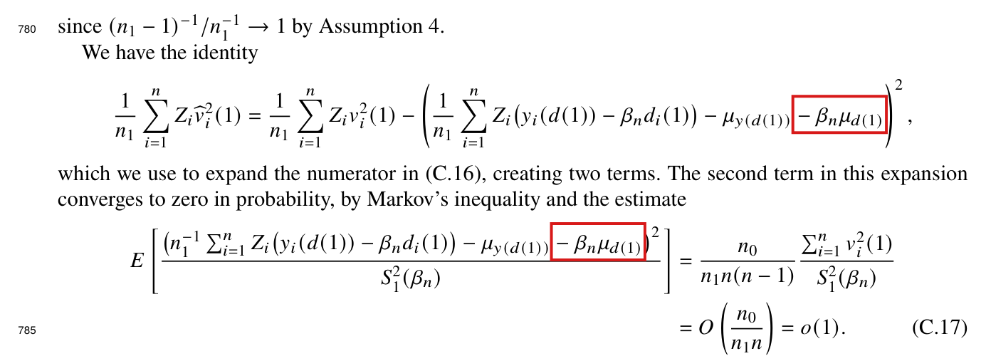
In the identity before (C.17) and in (C.17), the centering term is −μy(d(1))+βnμd(1)-\mu_{y(d(1))}+\beta_n\mu_{d(1)}; the sign of βnμd(1)\beta_n\mu_{d(1)} is printed wrong.

Supplement, proof of Lemma 7, p. 26 (PDF p. 6): the identity before (C.17) and the numerator of (C.17)

See also under Formal statements (Lean): P002-T10, P002-T11

As printed

We have the identity

1n1∑i=1nZiv^i2(1)=1n1∑i=1nZivi2(1)−(1n1∑i=1nZi(yi(d(1))−βndi(1))−μy(d(1))  −  βnμd(1))2,\frac1{n_1}\sum_{i=1}^nZ_i\widehat v_i^2(1)=\frac1{n_1}\sum_{i=1}^nZ_iv_i^2(1)-\left(\frac1{n_1}\sum_{i=1}^nZ_i\bigl(y_i(\colorbox{#ffe58a}{$\displaystyle d$}(1))-\beta_nd_i(1)\bigr)-\mu_{y(d(1))}\;\colorbox{#ffe58a}{$\displaystyle -$}\;\beta_n\mu_{d(1)}\right)^2,

which we use to expand the numerator in (C.16), creating two terms. The second term in this expansion converges to zero in probability, by Markov’s inequality and the estimate

E[(n1−1∑i=1nZi(yi(d(1))−βndi(1))−μy(d(1))  −  βnμd(1))2S12(βn)]=n0n1n(n−1)∑i=1nvi2(1)S12(βn)=O(n0n1n)=o(1).(C.17)\begin{aligned} E\left[\frac{\bigl(n_1^{-1}\sum_{i=1}^nZ_i\bigl(y_i(\colorbox{#ffe58a}{$\displaystyle d$}(1))-\beta_nd_i(1)\bigr)-\mu_{y(d(1))}\;\colorbox{#ffe58a}{$\displaystyle -$}\;\beta_n\mu_{d(1)}\bigr)^2}{S_1^2(\beta_n)}\right]&=\frac{n_0}{n_1n(n-1)}\frac{\sum_{i=1}^nv_i^2(1)}{S_1^2(\beta_n)}\\ &=O\left(\frac{n_0}{n_1n}\right)=o(1).\qquad\text{(C.17)} \end{aligned}
The problem

The quantity that is centered is wi=yi(di(1))−βndi(1)w_i=y_i(d_i(1))-\beta_nd_i(1), whose population mean is μy(d(1))−βnμd(1)\mu_{y(d(1))}-\beta_n\mu_{d(1)}. By (B.3), I have vi(1)=wi−μy(d(1))+βnμd(1)v_i(1)=w_i-\mu_{y(d(1))}+\beta_n\mu_{d(1)}. The term subtracted in the bracket is then μy(d(1))−βnμd(1)\mu_{y(d(1))}-\beta_n\mu_{d(1)}. With the printed sign the bracket is the error of the treated sample mean minus 2βnμd(1)2\beta_n\mu_{d(1)}. The identity is then false, and the expectation of the numerator in (C.17) exceeds the printed value by 4βn2μd(1)24\beta_n^2\mu_{d(1)}^2, which need not vanish. Both displays also print yi(d(1))y_i(d(1)) for yi(di(1))y_i(d_i(1)).

Evidence a derivation

The evidence is a derivation and an exact example. Set μw=μy(d(1))−βnμd(1)\mu_w=\mu_{y(d(1))}-\beta_n\mu_{d(1)} and wˉ1=n1−1∑iZiwi\bar w_1=n_1^{-1}\sum_iZ_iw_i. For a treated unit, v^i(1)=wi−wˉ1\widehat v_i(1)=w_i-\bar w_1 by equation (3) of the article and vi(1)=wi−μwv_i(1)=w_i-\mu_w by (B.3). Expanding the square, I obtain

1n1∑i=1nZiv^i2(1)=1n1∑i=1nZivi2(1)−(wˉ1−μw)2.\frac1{n_1}\sum_{i=1}^nZ_i\widehat v_i^2(1)=\frac1{n_1}\sum_{i=1}^nZ_iv_i^2(1)-(\bar w_1-\mu_w)^2.

Under complete randomization, I have E[wˉ1]=μwE[\bar w_1]=\mu_w and

var⁡(wˉ1)=n0n1n(n−1)∑i=1nvi2(1),\operatorname{var}(\bar w_1)=\frac{n_0}{n_1n(n-1)}\sum_{i=1}^nv_i^2(1),

which is the right side of (C.17) after division by S12(βn)S_1^2(\beta_n). For the example, set n=4n=4, n1=2n_1=2 and βn=2\beta_n=2, let all units be compliers with y(0)=(−1,−1,1,1)y(0)=(-1,-1,1,1) and y(1)=y(0)+2y(1)=y(0)+2, and treat the first two units. The left side of the identity is 00. The printed right side is 1−(−5)2=−241-(-5)^2=-24, and the corrected right side is 1−(−1)2=01-(-1)^2=0.

What survives

With the corrected sign the identity holds and (C.17) holds with its printed right side. Lemma 7 and the rest of its proof are unchanged, and no assumption is added.

Corrected

We have the identity

1n1∑i=1nZiv^i2(1)=1n1∑i=1nZivi2(1)−(1n1∑i=1nZi(yi(di(1))−βndi(1))−μy(d(1))  +  βnμd(1))2,\frac1{n_1}\sum_{i=1}^nZ_i\widehat v_i^2(1)=\frac1{n_1}\sum_{i=1}^nZ_iv_i^2(1)-\left(\frac1{n_1}\sum_{i=1}^nZ_i\bigl(y_i(\colorbox{#ffe58a}{$\displaystyle d_i$}(1))-\beta_nd_i(1)\bigr)-\mu_{y(d(1))}\;\colorbox{#ffe58a}{$\displaystyle +$}\;\beta_n\mu_{d(1)}\right)^2,

and the estimate

E[(n1−1∑i=1nZi(yi(di(1))−βndi(1))−μy(d(1))  +  βnμd(1))2S12(βn)]=n0n1n(n−1)∑i=1nvi2(1)S12(βn)=O(n0n1n)=o(1).(C.17)\begin{aligned} E\left[\frac{\bigl(n_1^{-1}\sum_{i=1}^nZ_i\bigl(y_i(\colorbox{#ffe58a}{$\displaystyle d_i$}(1))-\beta_nd_i(1)\bigr)-\mu_{y(d(1))}\;\colorbox{#ffe58a}{$\displaystyle +$}\;\beta_n\mu_{d(1)}\bigr)^2}{S_1^2(\beta_n)}\right]&=\frac{n_0}{n_1n(n-1)}\frac{\sum_{i=1}^nv_i^2(1)}{S_1^2(\beta_n)}\\ &=O\left(\frac{n_0}{n_1n}\right)=o(1).\qquad\text{(C.17)} \end{aligned}

Here μy(d(1))\mu_{y(d(1))} and μd(1)\mu_{d(1)} are the population means of yi(di(1))y_i(d_i(1)) and di(1)d_i(1).

Crop of two displays and the text between them. In the identity that begins with one over n1 times the sum of Z i times v-hat i squared, a red box marks the last term inside the large bracket, 'minus beta n mu d(1)'. In the numerator of the expectation in (C.17), a red box marks the same term.
Supplement, proof of Lemma 7, p. 26 (PDF p. 6): the identity before (C.17), and (C.17). The marked term −βnμd(1)-\beta_n\mu_{d(1)} should carry a plus sign in both displays.

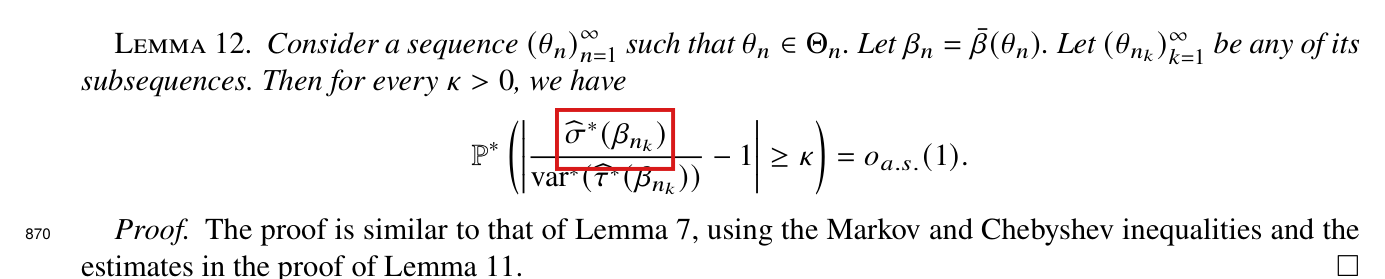
The numerator of the ratio in Lemma 12 is the estimated variance σ^∗2(βnk)\widehat\sigma^{*2}(\beta_{n_k}), and not the estimated standard deviation σ^∗(βnk)\widehat\sigma^{*}(\beta_{n_k}).

Supplementary Material, statement of Lemma 12, p. 30 (PDF p. 10 of the supplement)

See also under Formal statements (Lean): P002-T14, P002-T15

As printed

Lemma 12. Consider a sequence (θn)n=1∞(\theta_n)_{n=1}^\infty such that θn∈Θn\theta_n\in\Theta_n. Let βn=βˉ(θn)\beta_n=\bar\beta(\theta_n). Let (θnk)k=1∞(\theta_{n_k})_{k=1}^\infty be any of its subsequences. Then for every κ>0\kappa>0, we have

P∗(∣σ^∗(βnk)var⁡∗(τ^∗(βnk))−1∣≥κ)=oa.s.(1).\mathbb P^*\left(\left|\frac{\colorbox{#ffe58a}{$\displaystyle \widehat\sigma^*(\beta_{n_k})$}}{\operatorname{var}^*(\widehat\tau^*(\beta_{n_k}))}-1\right|\ge\kappa\right)=o_{a.s.}(1).
The problem

The ratio divides an estimated standard deviation by a variance. In the balanced, bounded-outcome example below, the denominator is of order 1/n1/n and σ^∗\widehat\sigma^* is of order n−1/2n^{-1/2}, so the printed ratio is of order n1/2n^{1/2} and does not approach 11. The sentence that introduces the lemma, the parallel statement in Lemma 7 and the use of the lemma to studentize in Lemma 13 all concern the ratio of the estimated variance to the variance.

Evidence a derivation

The evidence is an exact example in which the printed statement fails, and a derivation of the corrected one. Let nn be even and n1=n0=n/2n_1=n_0=n/2. Suppose that every unit is a complier with yi(1)=yi(0)y_i(1)=y_i(0), that half of these outcomes equal −1-1 and half equal 11, and that βn=0\beta_n=0. Let qq be the mean outcome in a reassigned treatment group, so that the control mean is −q-q. Computing the three quantities directly, I find

var⁡∗(τ^∗(0))=14(n−1),σ^∗2(0)=1−q24n,E∗q2=1n−1.\operatorname{var}^*(\widehat\tau^*(0))=\frac1{4(n-1)},\qquad\widehat\sigma^{*2}(0)=\frac{1-q^2}{4n},\qquad E^*q^2=\frac1{n-1}.

The printed ratio equals 2(n−1)n−1/2(1−q2)1/22(n-1)n^{-1/2}(1-q^2)^{1/2}, which diverges in P∗\mathbb P^*-probability for every original assignment. The ratio with the squared numerator is R=(n−1)(1−q2)/nR=(n-1)(1-q^2)/n. Since 0≤R≤10\le R\le1 and E∗(1−R)=2/nE^*(1-R)=2/n, Markov’s inequality implies that P∗(∣R−1∣≥κ)≤2/(nκ)\mathbb P^*(|R-1|\ge\kappa)\le2/(n\kappa). With κ=1/2\kappa=1/2 and n=8,32,128,512n=8,32,128,512, the exact probability for the printed ratio equals 11 up to rounding error in each case, and for the corrected ratio it is 0.0290.029, 4.9×10−54.9\times10^{-5}, 6.5×10−176.5\times10^{-17} and 1.6×10−631.6\times10^{-63}.

In general, let ai=Yi−βnDia_i=Y_i-\beta_nD_i minus its mean, S2=(n−1)−1∑iai2S^2=(n-1)^{-1}\sum_ia_i^2 and M2=max⁡iai2M^2=\max_ia_i^2. Lemma 11 implies that M2/(nS2)→0M^2/(nS^2)\to0 for almost every sequence of original assignments. In a reassigned arm of size mm, the mean of the ai2a_i^2 has expectation (n−1)S2/n(n-1)S^2/n and variance at most a constant times M2S2/nM^2S^2/n, and the squared arm mean has expectation O(S2/n)O(S^2/n). By Chebyshev’s and Markov’s inequalities, the centred second moment in each arm divided by S2S^2 tends to 11 in P∗\mathbb P^*-probability. Substituting into the definition of σ^∗2\widehat\sigma^{*2} on p. 6 of the article and comparing with (C.25), I obtain the corrected statement.

What survives

Lemma 13 and the studentized conditional central limit theorem use the ratio of variances and are unchanged. The correction needs no further assumption, and the coverage results are unaffected.

Corrected

Lemma 12. Consider a sequence (θn)n=1∞(\theta_n)_{n=1}^\infty such that θn∈Θn\theta_n\in\Theta_n. Let βn=βˉ(θn)\beta_n=\bar\beta(\theta_n). Let (θnk)k=1∞(\theta_{n_k})_{k=1}^\infty be any of its subsequences. Then for every κ>0\kappa>0, we have

P∗(∣σ^∗2(βnk)var⁡∗(τ^∗(βnk))−1∣≥κ)=oa.s.(1).\mathbb P^*\left(\left|\frac{\colorbox{#ffe58a}{$\displaystyle \widehat\sigma^{*2}(\beta_{n_k})$}}{\operatorname{var}^*(\widehat\tau^*(\beta_{n_k}))}-1\right|\ge\kappa\right)=o_{a.s.}(1).
Crop of the statement of Lemma 12 and the two lines of its proof. A red box marks the numerator of the ratio, sigma hat star of beta n k, printed without a square, above the denominator var star of tau hat star of beta n k.
Supplementary Material, p. 30 (PDF p. 10), Lemma 12. The marked numerator carries no square, while the denominator is a variance.

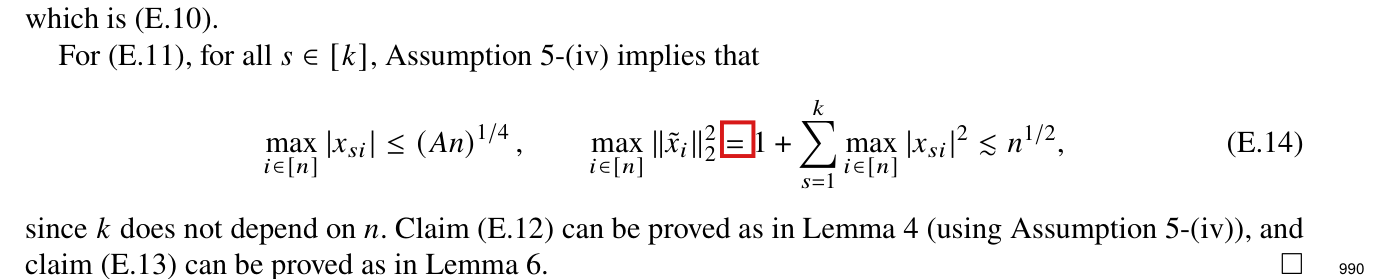
The middle relation in (E.14) is an inequality: the maximum over units of a sum is at most the sum of the maxima, and equality can fail.

Supplementary Material, proof of Lemma 16, display (E.14), p. 35 (PDF p. 15 of the supplement)

See also under Formal statements (Lean): P002-T16, P002-T17

As printed

For (E.11), for all s∈[k]s\in[k], Assumption 5-(iv) implies that

max⁡i∈[n]∣xsi∣≤(An)1/4,max⁡i∈[n]∥x~i∥22  =  1+∑s=1kmax⁡i∈[n]∣xsi∣2≲n1/2,(E.14)\max_{i\in[n]}|x_{si}|\le(An)^{1/4},\qquad\max_{i\in[n]}\|\tilde x_i\|_2^2\;\colorbox{#ffe58a}{$\displaystyle =$}\;1+\sum_{s=1}^k\max_{i\in[n]}|x_{si}|^2\lesssim n^{1/2},\qquad\text{(E.14)}

since kk does not depend on nn.

The problem

Since different coordinates can attain their maxima at different units, the two sides of the marked relation differ in general. Only the upper bound is used in the proof.

Evidence a derivation

The evidence is a derivation and an exact example. Since x~i=[1,xi′]′\tilde x_i=[1,x_i']', for every ii I have

∥x~i∥22=1+∑s=1k∣xsi∣2≤1+∑s=1kmax⁡j∈[n]∣xsj∣2,\|\tilde x_i\|_2^2=1+\sum_{s=1}^k|x_{si}|^2\le1+\sum_{s=1}^k\max_{j\in[n]}|x_{sj}|^2,

and I obtain the inequality by taking the maximum over ii. By Assumption 5-(iv), I have max⁡i∣xsi∣≤(An)1/4\max_i|x_{si}|\le(An)^{1/4}. The right-hand side is then at most 1+k(An)1/21+k(An)^{1/2}, which is O(n1/2)O(n^{1/2}) because kk is fixed. For the example, let k=2k=2 and n=4n=4, with the centred rows (1,0)(1,0), (−1,0)(-1,0), (0,1)(0,1) and (0,−1)(0,-1). The left-hand side equals 22 and the right-hand side equals 33.

What survives

The bound max⁡i∥x~i∥22≲n1/2\max_i\|\tilde x_i\|_2^2\lesssim n^{1/2}, claim (E.11) and Lemma 16 are unchanged.

Corrected

For (E.11), for all s∈[k]s\in[k], Assumption 5-(iv) implies that

max⁡i∈[n]∣xsi∣≤(An)1/4,max⁡i∈[n]∥x~i∥22  ≤  1+∑s=1kmax⁡i∈[n]∣xsi∣2≲n1/2,(E.14)\max_{i\in[n]}|x_{si}|\le(An)^{1/4},\qquad\max_{i\in[n]}\|\tilde x_i\|_2^2\;\colorbox{#ffe58a}{$\displaystyle \le$}\;1+\sum_{s=1}^k\max_{i\in[n]}|x_{si}|^2\lesssim n^{1/2},\qquad\text{(E.14)}

since kk does not depend on nn.

Crop of display (E.14) with the line before it and the two lines after it. A red box marks the equals sign between 'max over i of the squared norm of x tilde i' and '1 plus the sum over s of max over i of x s i squared'.
Supplementary Material, p. 35 (PDF p. 15), display (E.14). The marked sign equates the maximum of ∥x~i∥22\|\tilde x_i\|_2^2 with a sum of coordinatewise maxima.

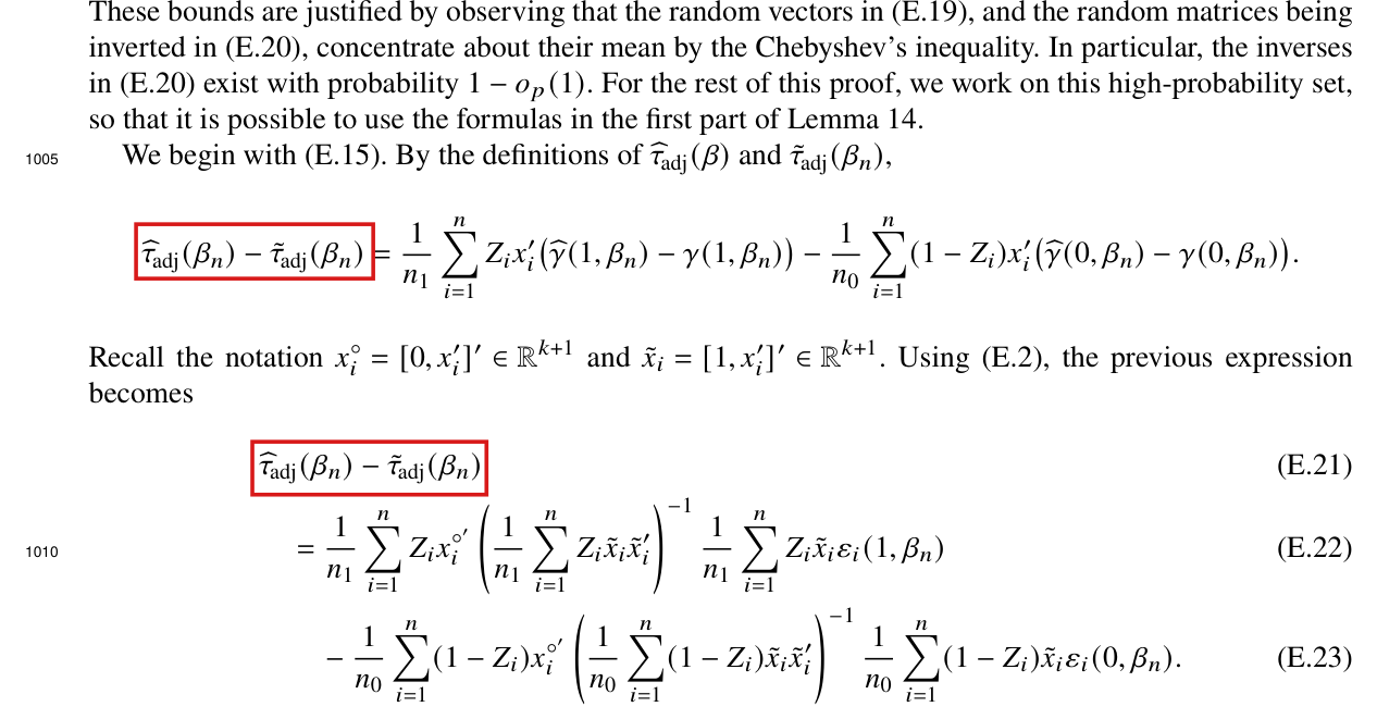
The difference τ^adj(βn)−τ~adj(βn)\widehat\tau_{\mathrm{adj}}(\beta_n)-\tilde\tau_{\mathrm{adj}}(\beta_n) is the negative of the right-hand side printed before (E.21) and in (E.21)–(E.23); the right-hand sides equal τ~adj(βn)−τ^adj(βn)\tilde\tau_{\mathrm{adj}}(\beta_n)-\widehat\tau_{\mathrm{adj}}(\beta_n).

Supplementary Material, proof of Lemma 17, the display before (E.21) and displays (E.21)–(E.23), p. 36 (PDF p. 16 of the supplement)

See also under Formal statements (Lean): P002-T18

As printed

We begin with (E.15). By the definitions of τ^adj(β)\widehat\tau_{\mathrm{adj}}(\beta) and τ~adj(βn)\tilde\tau_{\mathrm{adj}}(\beta_n),

τ^adj(βn)−τ~adj(βn)=1n1∑i=1nZixi′(γ^(1,βn)−γ(1,βn))−1n0∑i=1n(1−Zi)xi′(γ^(0,βn)−γ(0,βn)).\colorbox{#ffe58a}{$\displaystyle \widehat\tau_{\mathrm{adj}}(\beta_n)-\tilde\tau_{\mathrm{adj}}(\beta_n)$}=\frac1{n_1}\sum_{i=1}^nZ_ix_i'\big(\widehat\gamma(1,\beta_n)-\gamma(1,\beta_n)\big)-\frac1{n_0}\sum_{i=1}^n(1-Z_i)x_i'\big(\widehat\gamma(0,\beta_n)-\gamma(0,\beta_n)\big).

Recall the notation xi∘=[0,xi′]′∈Rk+1x_i^\circ=[0,x_i']'\in\mathbb R^{k+1} and x~i=[1,xi′]′∈Rk+1\tilde x_i=[1,x_i']'\in\mathbb R^{k+1}. Using (E.2), the previous expression becomes

τ^adj(βn)−τ~adj(βn)(E.21)=1n1∑i=1nZixi∘′(1n1∑i=1nZix~ix~i′)−11n1∑i=1nZix~iεi(1,βn)(E.22)−1n0∑i=1n(1−Zi)xi∘′(1n0∑i=1n(1−Zi)x~ix~i′)−11n0∑i=1n(1−Zi)x~iεi(0,βn).(E.23)\begin{aligned} &{}\colorbox{#ffe58a}{$\displaystyle \widehat\tau_{\mathrm{adj}}(\beta_n)-\tilde\tau_{\mathrm{adj}}(\beta_n)$}&&\text{(E.21)}\\ &\quad=\frac1{n_1}\sum_{i=1}^nZ_ix_i^{\circ\prime}\Big(\frac1{n_1}\sum_{i=1}^nZ_i\tilde x_i\tilde x_i'\Big)^{-1}\frac1{n_1}\sum_{i=1}^nZ_i\tilde x_i\varepsilon_i(1,\beta_n)&&\text{(E.22)}\\ &\quad\quad-\frac1{n_0}\sum_{i=1}^n(1-Z_i)x_i^{\circ\prime}\Big(\frac1{n_0}\sum_{i=1}^n(1-Z_i)\tilde x_i\tilde x_i'\Big)^{-1}\frac1{n_0}\sum_{i=1}^n(1-Z_i)\tilde x_i\varepsilon_i(0,\beta_n).&&\text{(E.23)} \end{aligned}
The problem

Both statistics subtract the fitted covariate term from the adjusted outcome, τ^adj\widehat\tau_{\mathrm{adj}} with the estimated slopes γ^\widehat\gamma and τ~adj\tilde\tau_{\mathrm{adj}} with the population slopes γ\gamma. Their difference carries a minus sign in the treated arm and a plus sign in the control arm, which is the opposite of what is printed. Substituting (E.2) and (E.3) does not change a sign, and (E.21)–(E.23) carry the same reversal.

Evidence a derivation

The evidence is a derivation from (9) of the article and (D.4). Subtracting (D.4) from (9), the terms Yi−βnDiY_i-\beta_nD_i cancel, and I obtain

τ^adj(βn)−τ~adj(βn)=−1n1∑i=1nZixi′(γ^(1,βn)−γ(1,βn))+1n0∑i=1n(1−Zi)xi′(γ^(0,βn)−γ(0,βn)).\widehat\tau_{\mathrm{adj}}(\beta_n)-\tilde\tau_{\mathrm{adj}}(\beta_n)=-\frac1{n_1}\sum_{i=1}^nZ_ix_i'\big(\widehat\gamma(1,\beta_n)-\gamma(1,\beta_n)\big)+\frac1{n_0}\sum_{i=1}^n(1-Z_i)x_i'\big(\widehat\gamma(0,\beta_n)-\gamma(0,\beta_n)\big).

Equations (E.2) and (E.3) express each slope error as the inverse of the arm design matrix applied to the sum of x~iεi\tilde x_i\varepsilon_i over the arm, with a positive sign. Substituting these expressions, I find (E.22) with a minus sign and (E.23) with a plus sign when the left-hand side is kept.

What survives

The proof uses only the absolute value of this difference, and claim (E.15) is stated for ∣τ~adj(βnk)−τ^adj(βnk)∣|\tilde\tau_{\mathrm{adj}}(\beta_{n_k})-\widehat\tau_{\mathrm{adj}}(\beta_{n_k})|. The bounds that follow, the other claims of Lemma 17 and the results on the confidence sets are unchanged.

Corrected

We begin with (E.15). By the definitions of τ^adj(β)\widehat\tau_{\mathrm{adj}}(\beta) and τ~adj(βn)\tilde\tau_{\mathrm{adj}}(\beta_n),

τ~adj(βn)−τ^adj(βn)=1n1∑i=1nZixi′(γ^(1,βn)−γ(1,βn))−1n0∑i=1n(1−Zi)xi′(γ^(0,βn)−γ(0,βn)).\colorbox{#ffe58a}{$\displaystyle \tilde\tau_{\mathrm{adj}}(\beta_n)-\widehat\tau_{\mathrm{adj}}(\beta_n)$}=\frac1{n_1}\sum_{i=1}^nZ_ix_i'\big(\widehat\gamma(1,\beta_n)-\gamma(1,\beta_n)\big)-\frac1{n_0}\sum_{i=1}^n(1-Z_i)x_i'\big(\widehat\gamma(0,\beta_n)-\gamma(0,\beta_n)\big).

Recall the notation xi∘=[0,xi′]′∈Rk+1x_i^\circ=[0,x_i']'\in\mathbb R^{k+1} and x~i=[1,xi′]′∈Rk+1\tilde x_i=[1,x_i']'\in\mathbb R^{k+1}. Using (E.2), the previous expression becomes

τ~adj(βn)−τ^adj(βn)(E.21)=1n1∑i=1nZixi∘′(1n1∑i=1nZix~ix~i′)−11n1∑i=1nZix~iεi(1,βn)(E.22)−1n0∑i=1n(1−Zi)xi∘′(1n0∑i=1n(1−Zi)x~ix~i′)−11n0∑i=1n(1−Zi)x~iεi(0,βn).(E.23)\begin{aligned} &{}\colorbox{#ffe58a}{$\displaystyle \tilde\tau_{\mathrm{adj}}(\beta_n)-\widehat\tau_{\mathrm{adj}}(\beta_n)$}&&\text{(E.21)}\\ &\quad=\frac1{n_1}\sum_{i=1}^nZ_ix_i^{\circ\prime}\Big(\frac1{n_1}\sum_{i=1}^nZ_i\tilde x_i\tilde x_i'\Big)^{-1}\frac1{n_1}\sum_{i=1}^nZ_i\tilde x_i\varepsilon_i(1,\beta_n)&&\text{(E.22)}\\ &\quad\quad-\frac1{n_0}\sum_{i=1}^n(1-Z_i)x_i^{\circ\prime}\Big(\frac1{n_0}\sum_{i=1}^n(1-Z_i)\tilde x_i\tilde x_i'\Big)^{-1}\frac1{n_0}\sum_{i=1}^n(1-Z_i)\tilde x_i\varepsilon_i(0,\beta_n).&&\text{(E.23)} \end{aligned}

Equivalently, the left-hand sides can be kept as printed and every right-hand side negated.

Crop of the start of the proof of claim (E.15) in Lemma 17: four lines of text, a display, two lines of text, and displays (E.21) to (E.23). Two red boxes mark the left-hand side 'tau hat adj of beta n minus tau tilde adj of beta n', once in the display before (E.21) and once in (E.21).
Supplementary Material, p. 36 (PDF p. 16), the display before (E.21) and displays (E.21)–(E.23). The marked left-hand sides are the difference whose sign is opposite to that of the right-hand sides.

Two signs in the proof of Lemma 18 are wrong: the right side of (E.41) lacks a minus sign, and the cross term displayed after (E.46) has coefficient −2-2, not 22; the residual in (E.41) also lacks its index ii.

Supplementary Material, proof of Lemma 18: display (E.41), p. 39 (PDF p. 19 of the supplement), and the unnumbered display after (E.46), p. 40 (PDF p. 20 of the supplement)

See also under Formal statements (Lean): P002-T19

As printed

Recalling the definition of x~i\tilde x_i, we have by a representation analogous to (E.2) that, asymptotically almost surely,

[φ(a,βn)−φ^(a,βn)γ(a,βn)−γ^(a,βn)]=(1na∑i∈T(a)x~ix~i′)−1(1na∑i∈T(a)x~iε(a,βn)).(E.41)\begin{bmatrix}\varphi(a,\beta_n)-\widehat\varphi(a,\beta_n)\\ \gamma(a,\beta_n)-\widehat\gamma(a,\beta_n)\end{bmatrix}\colorbox{#ffe58a}{$\displaystyle =$}\left(\frac{1}{n_a}\sum_{i\in\mathcal T(a)}\tilde x_i\tilde x_i'\right)^{-1}\left(\frac{1}{n_a}\sum_{i\in\mathcal T(a)}\tilde x_i\colorbox{#ffe58a}{$\displaystyle \varepsilon$}(a,\beta_n)\right).\qquad\text{(E.41)}

Next, (E.39) is, after applying (E.41),

2(1na∑i∈T(a)εi(a,βn)x~i′)(1na∑i∈T(a)x~ix~i′)−1(1na∑i∈T(a)x~iεi(a,βn)).\colorbox{#ffe58a}{$\displaystyle 2$}\left(\frac{1}{n_a}\sum_{i\in\mathcal T(a)}\varepsilon_i(a,\beta_n)\tilde x_i'\right)\left(\frac{1}{n_a}\sum_{i\in\mathcal T(a)}\tilde x_i\tilde x_i'\right)^{-1}\left(\frac{1}{n_a}\sum_{i\in\mathcal T(a)}\tilde x_i\varepsilon_i(a,\beta_n)\right).
The problem

Let ψ=(φ,γ′)′\psi=(\varphi,\gamma')' denote the population coefficients and ψ^\widehat\psi their least-squares estimates in arm aa. The least-squares identity (E.2)–(E.3) of Lemma 14 gives the difference ψ^−ψ\widehat\psi-\psi, estimate minus population. Display (E.41) prints the same right side for the difference ψ−ψ^\psi-\widehat\psi, which has the opposite sign. The term (E.39) carries the factor −2/na-2/n_a. When the correct identity is substituted into it, the resulting product has coefficient −2-2, and the display after (E.46) prints 22.

Evidence a derivation

The evidence is a derivation from the least-squares normal equations. Fix an arm aa and write

G=1na∑i∈T(a)x~ix~i′,h=1na∑i∈T(a)x~iεi(a,βn).G=\frac{1}{n_a}\sum_{i\in\mathcal T(a)}\tilde x_i\tilde x_i',\qquad h=\frac{1}{n_a}\sum_{i\in\mathcal T(a)}\tilde x_i\varepsilon_i(a,\beta_n).

For i∈T(a)i\in\mathcal T(a) the regressand is wi(a,βn)=x~i′ψ+εi(a,βn)w_i(a,\beta_n)=\tilde x_i'\psi+\varepsilon_i(a,\beta_n). The normal equations are

0=1na∑i∈T(a)x~i(wi(a,βn)−x~i′ψ^)=h−G(ψ^−ψ).0=\frac{1}{n_a}\sum_{i\in\mathcal T(a)}\tilde x_i\bigl(w_i(a,\beta_n)-\tilde x_i'\widehat\psi\bigr)=h-G(\widehat\psi-\psi).

When GG is invertible, the normal equations imply that ψ^−ψ=G−1h\widehat\psi-\psi=G^{-1}h and ψ−ψ^=−G−1h\psi-\widehat\psi=-G^{-1}h, in agreement with (E.2)–(E.3). Since xi′(γ^−γ)+φ^−φ=x~i′(ψ^−ψ)x_i'(\widehat\gamma-\gamma)+\widehat\varphi-\varphi=\tilde x_i'(\widehat\psi-\psi), I find that the term (E.39) equals −2h′(ψ^−ψ)=−2h′G−1h-2h'(\widehat\psi-\psi)=-2h'G^{-1}h.

The positive sign in (E.47) is not a further error. That display states that a quantity is oa.s.(1)o_{a.s.}(1), and a quantity is oa.s.(1)o_{a.s.}(1) exactly when its negative is.

What survives

The bounds (E.44), (E.46) and (E.47) and the conclusion (E.37) of Lemma 18 are unaffected, because they use only the fact that these quantities tend to zero. Only the two displays change.

Corrected

Recalling the definition of x~i\tilde x_i, we have by a representation analogous to (E.2) that, asymptotically almost surely,

[φ(a,βn)−φ^(a,βn)γ(a,βn)−γ^(a,βn)]=−(1na∑i∈T(a)x~ix~i′)−1(1na∑i∈T(a)x~iεi(a,βn)).(E.41)\begin{bmatrix}\varphi(a,\beta_n)-\widehat\varphi(a,\beta_n)\\ \gamma(a,\beta_n)-\widehat\gamma(a,\beta_n)\end{bmatrix}=\colorbox{#ffe58a}{$\displaystyle -$}\left(\frac{1}{n_a}\sum_{i\in\mathcal T(a)}\tilde x_i\tilde x_i'\right)^{-1}\left(\frac{1}{n_a}\sum_{i\in\mathcal T(a)}\tilde x_i\colorbox{#ffe58a}{$\displaystyle \varepsilon_i$}(a,\beta_n)\right).\qquad\text{(E.41)}

The identity holds whenever the matrix na−1∑i∈T(a)x~ix~i′n_a^{-1}\sum_{i\in\mathcal T(a)}\tilde x_i\tilde x_i' is invertible, which the proof shows to hold asymptotically almost surely.

Next, (E.39) is, after applying (E.41),

−2(1na∑i∈T(a)εi(a,βn)x~i′)(1na∑i∈T(a)x~ix~i′)−1(1na∑i∈T(a)x~iεi(a,βn)).\colorbox{#ffe58a}{$\displaystyle -2$}\left(\frac{1}{n_a}\sum_{i\in\mathcal T(a)}\varepsilon_i(a,\beta_n)\tilde x_i'\right)\left(\frac{1}{n_a}\sum_{i\in\mathcal T(a)}\tilde x_i\tilde x_i'\right)^{-1}\left(\frac{1}{n_a}\sum_{i\in\mathcal T(a)}\tilde x_i\varepsilon_i(a,\beta_n)\right).

The sign in (E.47) may be changed to match; its statement holds with either sign.

Crop of display (E.41): a column vector with entries phi(a, beta_n) minus phi-hat(a, beta_n) and gamma(a, beta_n) minus gamma-hat(a, beta_n), set equal to the inverse of an arm average of x-tilde_i x-tilde_i-prime times an arm average of x-tilde_i epsilon(a, beta_n). Red boxes mark the equality sign and the term epsilon(a, beta_n).
Supplementary Material, p. 39 (PDF p. 19 of the supplement): display (E.41). The right side, which begins after the marked equality sign, lacks a minus sign, and the marked residual ε(a,βn)\varepsilon(a,\beta_n) lacks its index ii.
Crop of the sentence 'Next, (E.39) is, after applying (E.41),' followed by a display: the number 2 times a product of three arm averages, the middle one inverted. A red box marks the leading 2.
Supplementary Material, p. 40 (PDF p. 20 of the supplement): the display after (E.46), which evaluates the cross term (E.39). The marked coefficient 22 should be −2-2.

The lower bound on the quadratic form holds with the constant min⁡{1,ε~}\min\{1,\tilde\varepsilon\} in place of ε~\tilde\varepsilon, because the matrix includes the intercept.

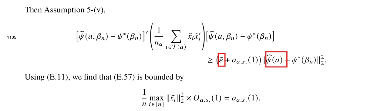
Supplement, proof of Lemma 19, p. 42 (PDF p. 22 of the Supplement), first display, after “Then Assumption 5-(v),”

See also under Formal statements (Lean): P002-T8, P002-T9

As printed

Then Assumption 5-(v),

[ψ^(a,βn)−ψ∗(βn)]′(1na∑i∈T(a)x~ix~i′)[ψ^(a,βn)−ψ∗(βn)]≥(ε~+oa.s.(1)) ∥ψ^(a)−ψ∗(βn)∥22.\begin{aligned} &\big[\widehat\psi(a,\beta_n)-\psi^*(\beta_n)\big]'\left(\frac{1}{n_a}\sum_{i\in\mathcal T(a)}\tilde x_i\tilde x_i'\right)\big[\widehat\psi(a,\beta_n)-\psi^*(\beta_n)\big]\\ &\qquad\qquad\ge\big(\colorbox{#ffe58a}{$\displaystyle \tilde\varepsilon$}+o_{a.s.}(1)\big)\,\|\colorbox{#ffe58a}{$\displaystyle \widehat\psi(a)$}-\psi^*(\beta_n)\|_2^2. \end{aligned}
The problem

Here x~i=[1,xi′]′\tilde x_i=[1,x_i']' is the covariate vector with an intercept. Assumption 5(v) bounds below by ε~\tilde\varepsilon the smallest eigenvalue of n−1∑i=1nxixi′n^{-1}\sum_{i=1}^n x_ix_i', the second-moment matrix of the covariates alone. Since the covariates are centred by Assumption 5(iii), the matrix n−1∑i=1nx~ix~i′n^{-1}\sum_{i=1}^n\tilde x_i\tilde x_i' has the additional eigenvalue 11 from the intercept, and its smallest eigenvalue is bounded below by min⁡{1,ε~}\min\{1,\tilde\varepsilon\}. Assumption 5 allows ε~>1\tilde\varepsilon>1, so the printed constant is justified only when ε~≤1\tilde\varepsilon\le1. The norm on the right-hand side also omits the argument βn\beta_n of ψ^\widehat\psi.

Evidence a derivation

The evidence is a derivation, with a counterexample to the printed step. Let Qn=n−1∑i=1nxixi′Q_n=n^{-1}\sum_{i=1}^n x_ix_i'. By Assumption 5(iii), I have n−1∑i=1nx~ix~i′=diag⁡(1,Qn)n^{-1}\sum_{i=1}^n\tilde x_i\tilde x_i'=\operatorname{diag}(1,Q_n), and λmin⁡(Qn)≥ε~\lambda_{\min}(Q_n)\ge\tilde\varepsilon by Assumption 5(v). The smallest eigenvalue of diag⁡(1,Qn)\operatorname{diag}(1,Q_n) is min⁡{1,λmin⁡(Qn)}\min\{1,\lambda_{\min}(Q_n)\}, which is at least min⁡{1,ε~}\min\{1,\tilde\varepsilon\}. By (E.40), the matrix na−1∑i∈T(a)x~ix~i′n_a^{-1}\sum_{i\in\mathcal T(a)}\tilde x_i\tilde x_i' equals diag⁡(1,Qn)+oa.s.(1)\operatorname{diag}(1,Q_n)+o_{a.s.}(1). Weyl’s inequality then implies that its smallest eigenvalue is at least min⁡{1,ε~}+oa.s.(1)\min\{1,\tilde\varepsilon\}+o_{a.s.}(1), and the corrected bound follows for every vector in place of ψ^(a,βn)−ψ∗(βn)\widehat\psi(a,\beta_n)-\psi^*(\beta_n).

For the counterexample, suppose that there is a single covariate, whose values alternate between 22 and −2-2, so that Qn=4Q_n=4, and let ε~=2\tilde\varepsilon=2 and v=(1,0)′v=(1,0)'. Then

v′diag⁡(1,4) v=1<2=ε~ ∥v∥22.v'\operatorname{diag}(1,4)\,v=1<2=\tilde\varepsilon\,\|v\|_2^2.

The matrix diag⁡(1,Qn)\operatorname{diag}(1,Q_n) does not satisfy the bound with the constant ε~\tilde\varepsilon. This does not contradict Lemma 19.

What survives

The step needs only a lower bound by a fixed positive constant, and min⁡{1,ε~}\min\{1,\tilde\varepsilon\} is such a constant. The bound on (E.57), Lemma 19 and the results that rest on it hold under the assumptions as stated.

Corrected

Then Assumption 5-(v),

[ψ^(a,βn)−ψ∗(βn)]′(1na∑i∈T(a)x~ix~i′)[ψ^(a,βn)−ψ∗(βn)]≥(min⁡{1,ε~}+oa.s.(1)) ∥ψ^(a,βn)−ψ∗(βn)∥22.\begin{aligned} &\big[\widehat\psi(a,\beta_n)-\psi^*(\beta_n)\big]'\left(\frac{1}{n_a}\sum_{i\in\mathcal T(a)}\tilde x_i\tilde x_i'\right)\big[\widehat\psi(a,\beta_n)-\psi^*(\beta_n)\big]\\ &\qquad\qquad\ge\big(\colorbox{#ffe58a}{$\displaystyle \min\{1,\tilde\varepsilon\}$}+o_{a.s.}(1)\big)\,\|\widehat\psi(a\colorbox{#ffe58a}{$\displaystyle ,\beta_n$})-\psi^*(\beta_n)\|_2^2. \end{aligned}

Here a∈{0,1}a\in\{0,1\}, x~i=[1,xi′]′\tilde x_i=[1,x_i']', and ε~>0\tilde\varepsilon>0 is the constant of Assumption 5(v), on which no upper bound is imposed. The bound uses Assumption 5(iii), ∑i=1nxi=0k\sum_{i=1}^nx_i=0_k, and (E.40) together with Assumption 5(v).

The display that follows the words Then Assumption 5-(v): a quadratic form in the difference of psi-hat(a, beta-n) and psi-star(beta-n) is bounded below by epsilon-tilde plus an almost surely vanishing term, times a squared norm. Red outlines mark epsilon-tilde and the term psi-hat(a) inside the norm. Below, the text continues: Using (E.11), we find that (E.57) is bounded by, with a further display.
Supplement, p. 42 (PDF p. 22 of the Supplement), first display, in the proof of Lemma 19. Outlined: the constant ε~\tilde\varepsilon, and ψ^(a)\widehat\psi(a) printed without its argument βn\beta_n.

The inner supremum of (E.36) is taken over Θn\Theta_n, the parameter space of the theory without covariates; it should be taken over Ξn\Xi_n, the parameter space of the regression-adjusted theory. If the population size ranges over all positive integers, the inner limit should also be a limit superior.

Supplementary Material, Theorem 7, display (E.36), p. 39 (PDF p. 19 of the supplement), inner supremum

See also under Formal statements (Lean): P002-T21

Revised: see the history of this entry.

As printed

Theorem 7. For every α∈(0,1)\alpha\in(0,1),

lim⁡κ→0+lim⁡n→∞sup⁡β∈R sup⁡{θ∈Θn: βˉ(θ)=β}Pθ(∣Δadj(β)∣>z1−α/2−κ)≤α.(E.36)\lim_{\kappa\to0^+}\lim_{n\to\infty}\sup_{\beta\in\mathbb R}\ \sup_{\{\theta\in\colorbox{#ffe58a}{$\displaystyle \scriptstyle\Theta_n$}:\,\bar\beta(\theta)=\beta\}}\mathbb P_\theta\bigl(\lvert\Delta_{\mathrm{adj}}(\beta)\rvert>z_{1-\alpha/2}-\kappa\bigr)\le\alpha.\qquad\text{(E.36)}
The problem

The space Θn\Theta_n collects the models without covariates that satisfy Assumptions 1–4 (p. 7 of the article). Theorem 7 concerns the regression-adjusted statistic Δadj\Delta_{\mathrm{adj}}. Section D.1 of the Supplementary Material fixes Ξn=Ξn(k,δ,ε~,A,B,r)\Xi_n=\Xi_n(k,\delta,\tilde\varepsilon,A,B,r), the parameter space of Theorem 2, for Sections D and E, and the proof of Theorem 7 rests on Lemma 17, which is stated for sequences θn∈Ξn\theta_n\in\Xi_n.

There is also an issue with the inner limit. Assumption 4 (p. 7 of the article) allows r=1/2r=1/2, which forces n1=n/2n_1=n/2, so both Θn\Theta_n and Ξn\Xi_n are empty at every odd population size. The paper neither restricts the size index to feasible sizes nor says what value an empty supremum of probabilities takes. If that value is zero, the inner limit can fail to exist, even for κ\kappa arbitrarily close to zero. Take mm units in each of the four cells (xi,zi)∈{−1,1}2(x_i,z_i)\in\{-1,1\}^2, all compliers, with yi(0)=yi(1)=ziy_i(0)=y_i(1)=z_i and n1=n/2n_1=n/2; these models belong to Ξn\Xi_n with k=1k=1, δ=0\delta=0, ε~=1/2\tilde\varepsilon=1/2 and A=B=2A=B=2. For α=1/2\alpha=1/2 and every 0<κ<z1−α/20<\kappa<z_{1-\alpha/2}, the rejection probability tends to 2{1−Φ(z1−α/2−κ)}>1/22\{1-\Phi(z_{1-\alpha/2}-\kappa)\}>1/2 along the sizes divisible by four, where Φ\Phi is the standard normal distribution function, while the supremum is zero at every odd size. The argument of Lemma 17 and Theorem 6 bounds the limit superior; it does not show that the ordinary inner limit exists. Restricting the index to feasible sizes removes this example but would need its own argument for existence.

Evidence a check of the printed page

The evidence is a check of the pages: the definitions of Θn\Theta_n (p. 7) and of Ξn\Xi_n (p. 11) in the article, and Section D.1 (p. 31) and the statement of Lemma 17 (p. 35) in the Supplementary Material. I checked the four-cell example by exact enumeration of the assignment distribution for n=4n=4, 88 and 1212.

What survives

The model-space correction and the conservative bound on the adjusted tail are retained in the limit-superior form below. That the ordinary inner limits exist is not established.

Corrected

Theorem 7. For every α∈(0,1)\alpha\in(0,1),

lim⁡κ→0+lim sup⁡n→∞sup⁡β∈R sup⁡{θ∈Ξn: βˉ(θ)=β}Pθ(∣Δadj(β)∣>z1−α/2−κ)≤α.(E.36)\lim_{\kappa\to0^+}\colorbox{#ffe58a}{$\displaystyle \limsup_{n\to\infty}$}\sup_{\beta\in\mathbb R}\ \sup_{\{\theta\in\colorbox{#ffe58a}{$\displaystyle \scriptstyle\Xi_n$}:\,\bar\beta(\theta)=\beta\}}\mathbb P_\theta\bigl(\lvert\Delta_{\mathrm{adj}}(\beta)\rvert>z_{1-\alpha/2}-\kappa\bigr)\le\alpha.\qquad\text{(E.36)}

Here Ξn=Ξn(k,δ,ε~,A,B,r)\Xi_n=\Xi_n(k,\delta,\tilde\varepsilon,A,B,r) is the parameter space of models that satisfy Assumptions 1, 2, 4 and 5, with the constants fixed in the statement of Theorem 2, as in Section D.1 of the Supplementary Material. The population size ranges over all positive integers, and an empty supremum of probabilities is zero. The outer limit exists because the inner limit superior is nondecreasing in κ\kappa and lies in [0,1][0,1].

Crop of Theorem 7: 'For every alpha in (0, 1)', followed by display (E.36), a double limit of a supremum over beta and a supremum over theta in Theta_n with beta-bar(theta) equal to beta, of the probability that the absolute value of Delta_adj(beta) exceeds z_(1 - alpha/2) minus kappa, bounded by alpha. A red box marks Theta_n in the subscript of the inner supremum. The proof below reads 'Given Lemma 17, the proof of (E.36) is nearly identical to the proof of Theorem 6, so we omit it.'
Supplementary Material, p. 39 (PDF p. 19 of the supplement): Theorem 7 and the first lines of its proof. The marked symbol Θn\Theta_n under the inner supremum of (E.36) should be Ξn\Xi_n.
History of this entry
  1. Classification before my review (the classification when the audit was first completed, before I reviewed it): Minor error.
  2. Revised. The wording was revised; the classification is unchanged. How this came to light: stating Theorem 7 in Lean showed that the display asserts an ordinary inner limit, and that with r=1/2r=1/2 the model classes are empty at every odd population size. Admissible models exist whose rejection probabilities stay above one half along the sizes divisible by four, for every κ\kappa near zero, while the supremum is zero at odd sizes. Why it changed: the correction had said that only the symbol changes and that Theorem 2 is unaffected; neither assurance holds as stated. The corrected display now uses a limit superior, which the argument of the paper supports. P. M. Aronow delegated this decision to the model session that runs the audit, which adopted the amendment recommended by the two checks; this note was written by that session.

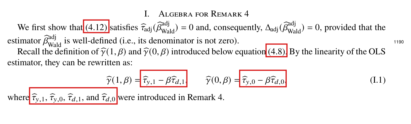
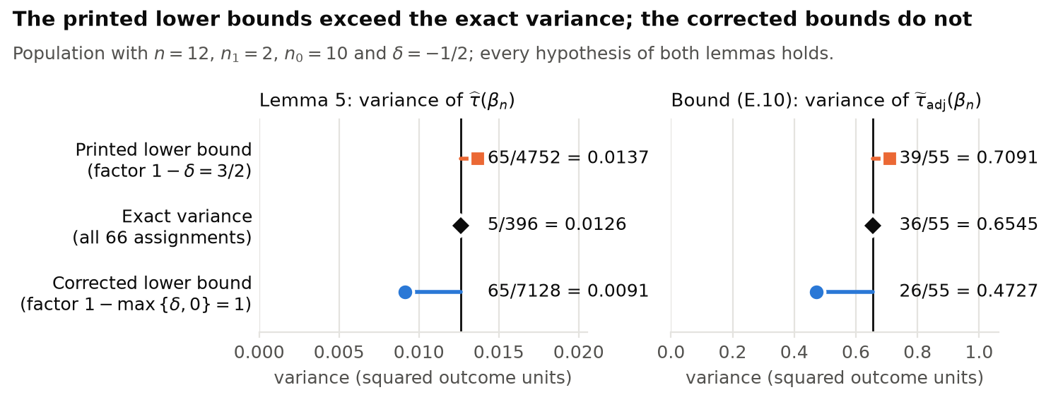
Several cross-references point to the wrong place: the Supplementary Material cites equations of the article by section-prefixed numbers that the article does not use, Theorem 3 places Assumption 6 in the Supplementary Material, two steps in the proof of Lemma 16 cite the wrong parts of Assumption 5, its covariance and variance bounds can fail for allowed negative δ\delta, and displays (I.1) and (I.2) write the regression slopes of Remark 4 as τ^\widehat\tau.

Theorem 3, p. 17; Supplementary Material, pp. 23, 25, 32, 34, 35, 42, 43, 45, 46 and 48 (PDF pp. 3, 5, 12, 14, 15, 22, 23, 25, 26 and 28 of the supplement)

See also under Formal statements (Lean): P002-T24, P002-T28

As printed
  • Theorem 3, p. 17: “Without covariates and under Assumption 6 in the Supplementary Material, the confidence set CS returned by Algorithm 1 or 2 is equal to that in (14).”
  • Supplementary Material, pointers to equations of the article: “following (2.2)” (p. 23); “recalling the definitions in (3.3)” (p. 25); “between expressions (4.9) and (D.4)” (p. 32); “similar to (5.15) and (5.16)” (p. 42); “the definition of Δadj(β)\Delta_{\mathrm{adj}}(\beta) from (4.10)” (p. 43); “the definition of I\mathcal I in (5.17)”, “the confidence set defined in (5.14)”, “We first show that (4.12) satisfies” and “introduced below equation (4.8)” (p. 45); “generated according to (6.18) and (6.19)” and “generated according to (6.20) and (6.21)” (p. 48).
  • Lemma 16, p. 34:
    var⁡(τ~adj(βnk))≥(1−δ)n0n1nS12(βnk)+(1−δ)n1n0nS02(βnk).(E.10)\operatorname{var}\big(\widetilde\tau_{\mathrm{adj}}(\beta_{n_k})\big)\ge(1-\colorbox{#ffe58a}{$\displaystyle \delta$})\frac{n_0}{n_1n}S_1^2(\beta_{n_k})+(1-\colorbox{#ffe58a}{$\displaystyle \delta$})\frac{n_1}{n_0n}S_0^2(\beta_{n_k}).\qquad\text{(E.10)}
    Its proof, p. 35, uses
    ∑i=1n(εi(1,βn)−εi(0,βn))2=∑i=1nεi2(1,βn)+∑i=1nεi2(0,βn)−2∑i=1nεi(1,βn)εi(0,βn)≤(1+δn0n1)∑i=1nεi2(1,βn)+(1+δn1n0)∑i=1nεi2(0,βn),\begin{aligned} \sum_{i=1}^n\big(\varepsilon_i(1,\beta_n)-\varepsilon_i(0,\beta_n)\big)^2 &=\sum_{i=1}^n\varepsilon_i^2(1,\beta_n)+\sum_{i=1}^n\varepsilon_i^2(0,\beta_n)-2\sum_{i=1}^n\varepsilon_i(1,\beta_n)\varepsilon_i(0,\beta_n)\\ &\le\Big(1+\frac{\colorbox{#ffe58a}{$\displaystyle \delta$}n_0}{n_1}\Big)\sum_{i=1}^n\varepsilon_i^2(1,\beta_n)+\Big(1+\frac{\colorbox{#ffe58a}{$\displaystyle \delta$}n_1}{n_0}\Big)\sum_{i=1}^n\varepsilon_i^2(0,\beta_n), \end{aligned}
    followed by “where the inequality follows from Assumption 5-(ii)”, and ends with “Claim (E.12) can be proved as in Lemma 4 (using Assumption 5-(iv))”.
  • Section I, p. 45:
    γ^(1,β)=τ^y,1−β τ^d,1,γ^(0,β)=τ^y,0−β τ^d,0,(I.1)\widehat\gamma(1,\beta)=\colorbox{#ffe58a}{$\displaystyle \widehat\tau_{y,1}$}-\beta\,\colorbox{#ffe58a}{$\displaystyle \widehat\tau_{d,1}$},\qquad\widehat\gamma(0,\beta)=\colorbox{#ffe58a}{$\displaystyle \widehat\tau_{y,0}$}-\beta\,\colorbox{#ffe58a}{$\displaystyle \widehat\tau_{d,0}$},\qquad\text{(I.1)}
    “where τ^y,1\widehat\tau_{y,1}, τ^y,0\widehat\tau_{y,0}, τ^d,1\widehat\tau_{d,1}, and τ^d,0\widehat\tau_{d,0} were introduced in Remark 4.” The same symbols recur in (I.2) and in the text after it.
  • Section I, p. 46: “The quantity τ^(β)\colorbox{#ffe58a}{$\widehat\tau(\beta)$} can be rewritten as”, followed by a display for τ^adj(β)\widehat\tau_{\mathrm{adj}}(\beta).
The problem

The article numbers its equations (1) to (21), and the numbers with a section prefix that the Supplementary Material cites do not exist in it. Assumption 6 is stated in Section 5.2 of the article, p. 14; the Supplementary Material states only Assumption 7. In the proof of Lemma 16, the inequality that leads to (E.10) uses a bound on the sum of products of the residuals εi(1,βn)εi(0,βn)\varepsilon_i(1,\beta_n)\varepsilon_i(0,\beta_n), which is the subject of the correlation bound 5-(i) and not of the fourth-moment bound 5-(ii). Changing this pointer alone is insufficient: the printed inequality and (E.10) can fail when δ<0\delta<0, which Assumption 5 permits. Claim (E.12) concerns the largest squared residual, which is the subject of 5-(ii) and not of the covariate bound 5-(iv). Remark 4 introduces the slopes γ^y,1\widehat\gamma_{y,1}, γ^y,0\widehat\gamma_{y,0}, γ^d,1\widehat\gamma_{d,1} and γ^d,0\widehat\gamma_{d,0}, and no symbols τ^y,z\widehat\tau_{y,z} or τ^d,z\widehat\tau_{d,z}. Each intended target can be recovered from the content.

Evidence a derivation

I checked the pages and the bounds, including an exact counterexample. The targets of the equation pointers are:

Pointers in the Supplementary Material to equations of the article.
Printed page of the supplementPrinted pointerEquation of the article
23(2.2)(2)
25(3.3)(3)
32(4.9)(9)
42(5.15), (5.16)(15), (16)
43(4.10)(10)
45(5.17), (5.14), (4.12), (4.8)(17), (14), (12), (8)
48(6.18), (6.19), (6.20), (6.21)(18), (19), (20), (21)

For the first step of Lemma 16, let U=∑iεi2(1,βn)U=\sum_i\varepsilon_i^2(1,\beta_n), W=∑iεi2(0,βn)W=\sum_i\varepsilon_i^2(0,\beta_n) and C=∑iεi(1,βn)εi(0,βn)C=\sum_i\varepsilon_i(1,\beta_n)\varepsilon_i(0,\beta_n). The residuals have mean zero, and Assumption 5-(i) implies that C≥−δ(UW)1/2C\ge-\delta(UW)^{1/2}. Set δ+=max⁡{δ,0}\delta_+=\max\{\delta,0\}. Then C≥−δ+(UW)1/2C\ge-\delta_+(UW)^{1/2}, and since δ+≥0\delta_+\ge0 and 2(UW)1/2≤(n0/n1)U+(n1/n0)W2(UW)^{1/2}\le(n_0/n_1)U+(n_1/n_0)W, I have

U+W−2C≤(1+δ+n0n1)U+(1+δ+n1n0)W.U+W-2C\le\Big(1+\frac{\delta_+n_0}{n_1}\Big)U+\Big(1+\frac{\delta_+n_1}{n_0}\Big)W.

This yields (E.10) with 1−δ+1-\delta_+ in place of 1−δ1-\delta. To see why the replacement is needed, take n=6n=6, n1=2n_1=2, n0=4n_0=4, δ=−9/10\delta=-9/10, all compliers, x=(1,−1,1,−1,0,0)x=(1,-1,1,-1,0,0) and y(0)=y(1)=(1,1,−1,−1,0,0)y(0)=y(1)=(1,1,-1,-1,0,0). These satisfy the stated assumptions with r=1/3r=1/3, ε~=1/2\widetilde\varepsilon=1/2, A=1A=1 and B=2B=2, and give β‾=0\overline\beta=0 and U=W=C=4U=W=C=4: the printed inequality reads 0≤−10\le-1, and (E.10) claims the variance 3/53/5 is at least 19/3019/30. For (E.12), Assumption 5-(ii) gives max⁡iεi2(a,βn)≤{∑iεi4(a,βn)}1/2≤B2n1/2σε(a,βn)2\max_i\varepsilon_i^2(a,\beta_n)\le\{\sum_i\varepsilon_i^4(a,\beta_n)\}^{1/2}\le B^2n^{1/2}\sigma^2_{\varepsilon(a,\beta_n)}, and n−1∑iεi2(a,βn)=(n−1)σε(a,βn)2/nn^{-1}\sum_i\varepsilon_i^2(a,\beta_n)=(n-1)\sigma^2_{\varepsilon(a,\beta_n)}/n. The ratio in (E.12) is then at most B2n3/2/(n−1)B^2n^{3/2}/(n-1), which is o(n)o(n). The use of Assumption 5-(iv) for (E.14) is correct. For (I.1), the outcome Yi−βDiY_i-\beta D_i is linear in (Yi,Di)(Y_i,D_i) and the regressions share one design. The fitted slope is then γ^y,a−βγ^d,a\widehat\gamma_{y,a}-\beta\widehat\gamma_{d,a}.

What survives

The definitions and regression algebra are unaffected. The variance lower bound (E.10) and its uses need 1−δ+1-\delta_+, which remains strictly positive throughout the stated range δ<1\delta<1.

Corrected
  • Theorem 3: “Without covariates and under Assumption 6, the confidence set CS returned by Algorithm 1 or 2 is equal to that in (14).” The reference to the Supplementary Material after Assumption 7 stays.
  • In the Supplementary Material, replace (2.2), (3.3), (4.8), (4.9), (4.10), (4.12), (5.14), (5.15), (5.16), (5.17), (6.18), (6.19), (6.20) and (6.21) by (2), (3), (8), (9), (10), (12), (14), (15), (16), (17), (18), (19), (20) and (21).
  • Lemma 16 and its proof: define δ+=max⁡{δ,0}\delta_+=\max\{\delta,0\} and replace δ\delta by δ+\colorbox{#ffe58a}{$\delta_+$} in the covariance inequality, the ensuing variance bounds including (E.10), and subsequent uses of this lower bound. The pointer sentences become “where the inequality follows from Assumption 5-(i)” and “Claim (E.12) can be proved as in Lemma 4 (using Assumption 5-(ii))”.
  • Section I:
    γ^(1,β)=γ^y,1−β γ^d,1,γ^(0,β)=γ^y,0−β γ^d,0,(I.1)\widehat\gamma(1,\beta)=\colorbox{#ffe58a}{$\displaystyle \widehat\gamma_{y,1}$}-\beta\,\colorbox{#ffe58a}{$\displaystyle \widehat\gamma_{d,1}$},\qquad\widehat\gamma(0,\beta)=\colorbox{#ffe58a}{$\displaystyle \widehat\gamma_{y,0}$}-\beta\,\colorbox{#ffe58a}{$\displaystyle \widehat\gamma_{d,0}$},\qquad\text{(I.1)}
    “where γ^y,1\widehat\gamma_{y,1}, γ^y,0\widehat\gamma_{y,0}, γ^d,1\widehat\gamma_{d,1}, and γ^d,0\widehat\gamma_{d,0} were introduced in Remark 4.” The same replacement applies in (I.2) and in the text after it.
  • Section I, p. 46: “The quantity τ^adj(β)\colorbox{#ffe58a}{$\widehat\tau_{\mathrm{adj}}(\beta)$} can be rewritten as”.
Crop of the statement of Theorem 3. A red box marks the words 'in the Supplementary Material' that follow 'Without covariates and under Assumption 6'.
Theorem 3, p. 17. The marked phrase places Assumption 6 in the Supplementary Material; it is stated in Section 5.2 of the article, p. 14.
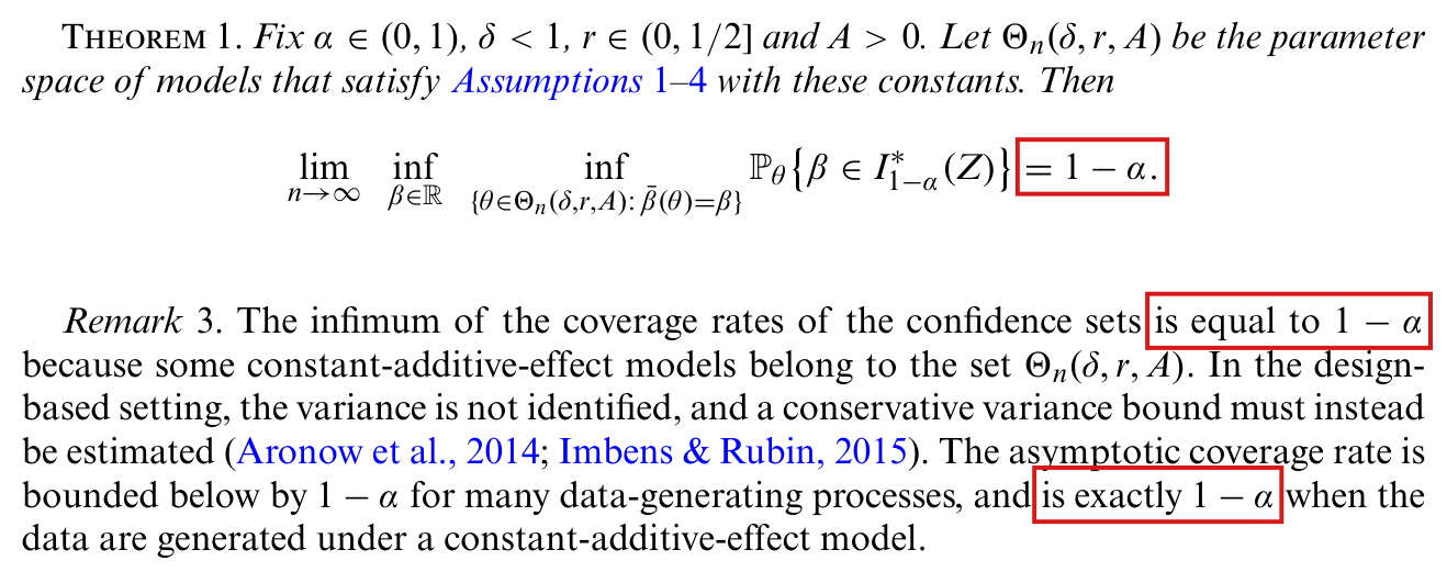
Crop of the last line of a displayed inequality and the sentence after it. A red box marks 'Assumption 5-(ii)' in 'where the inequality follows from Assumption 5-(ii). Therefore, recalling (D.5),'.
Supplementary Material, p. 35 (PDF p. 15), proof of Lemma 16. The marked pointer should be to Assumption 5-(i); the printed inequality follows for δ≥0\delta\ge0, but needs δ+=max⁡{δ,0}\delta_+=\max\{\delta,0\} in place of δ\delta over the full stated range.
Crop of display (E.14) and the two lines after it. A red box marks '(using Assumption 5-(iv))' in 'Claim (E.12) can be proved as in Lemma 4 (using Assumption 5-(iv)), and claim (E.13) can be proved as in Lemma 6'.
Supplementary Material, p. 35 (PDF p. 15), end of the proof of Lemma 16. The marked pointer is given for claim (E.12), which concerns residuals and follows from Assumption 5-(ii).
Crop of the first lines of Section I, Algebra for Remark 4, to display (I.1) and the sentence after it. Red boxes mark '(4.12)' in 'We first show that (4.12) satisfies', '(4.8)' in 'introduced below equation (4.8)', the two right-hand sides of display (I.1), 'tau hat y,1 minus beta tau hat d,1' and 'tau hat y,0 minus beta tau hat d,0', and the four symbols 'tau hat y,1, tau hat y,0, tau hat d,1, and tau hat d,0' in the sentence 'were introduced in Remark 4'.
Supplementary Material, p. 45 (PDF p. 25), start of Section I. The marked pointers (4.12) and (4.8) are to equations (12) and (8) of the article, and the marked symbols τ^y,z\widehat\tau_{y,z}, τ^d,z\widehat\tau_{d,z} are the slopes that Remark 4 calls γ^y,z\widehat\gamma_{y,z}, γ^d,z\widehat\gamma_{d,z}.
Crop of the first line of printed page 46 and the first line of the display after it. A red box marks 'tau hat of beta' in 'The quantity tau hat of beta can be rewritten as'; the display below begins 'tau hat adj of beta equals'.
Supplementary Material, p. 46 (PDF p. 26). The marked symbol lacks the subscript of the statistic τ^adj(β)\widehat\tau_{\mathrm{adj}}(\beta) that the display defines.

In the second and third lines of (H.1) the critical value η^1−α∗(β,Z)\widehat\eta^*_{1-\alpha}(\beta,Z) should be squared, since it is compared with the squared statistic.

Supplement, Section H.2, display (H.1), second and third lines, p. 45 (PDF p. 25 of the Supplement)

See also under Formal statements (Lean): P002-T23

As printed
CSi={β:∣Δ2(β)∣≤∣Δmi∗2(β)∣, β∈[βi,βi+1]}={β:∣Δ2(β)∣≤η^1−α∗(β,Z), β∈[βi,βi+1]}={β:∣Δ2(β)∣≤η^1−α∗(β,Z)}∩[βi,βi+1]=CS∗∩[βi,βi+1],(H.1)\begin{aligned} \mathrm{CS}_i&=\big\{\beta:|\Delta^2(\beta)|\le|\Delta^{*2}_{m_i}(\beta)|,\ \beta\in[\beta_i,\beta_{i+1}]\big\}\\ &=\big\{\beta:|\Delta^2(\beta)|\le\colorbox{#ffe58a}{$\displaystyle \widehat\eta^*_{1-\alpha}(\beta,Z)$},\ \beta\in[\beta_i,\beta_{i+1}]\big\}\\ &=\big\{\beta:|\Delta^2(\beta)|\le\colorbox{#ffe58a}{$\displaystyle \widehat\eta^*_{1-\alpha}(\beta,Z)$}\big\}\cap[\beta_i,\beta_{i+1}]\\ &=\mathrm{CS}^*\cap[\beta_i,\beta_{i+1}],\qquad\qquad\text{(H.1)} \end{aligned}

where the second equality is justified by Lemma 1.

The problem

By (13) of the article, η^1−α∗(β,Z)\widehat\eta^*_{1-\alpha}(\beta,Z) is an empirical quantile of the simulated absolute values ∣Δm∗(β)∣|\Delta^*_m(\beta)|, and the confidence set CS∗\mathrm{CS}^* of (14) compares ∣Δ(β)∣|\Delta(\beta)| with it. The first line of (H.1) compares the squared statistic with a squared simulated statistic. The second and third lines keep the square on Δ\Delta and omit it on the critical value. As printed, the sets in these two lines do not equal CS∗∩[βi,βi+1]\mathrm{CS}^*\cap[\beta_i,\beta_{i+1}] in general.

Evidence a derivation

The evidence is a derivation. By Lemma 1, there exists an index mim_i such that, on [βi,βi+1][\beta_i,\beta_{i+1}], I have η^1−α∗(β,Z)=∣Δmi∗(β)∣\widehat\eta^*_{1-\alpha}(\beta,Z)=|\Delta^*_{m_i}(\beta)|, so that ∣Δmi∗2(β)∣=[η^1−α∗(β,Z)]2|\Delta^{*2}_{m_i}(\beta)|=\big[\widehat\eta^*_{1-\alpha}(\beta,Z)\big]^2. For nonnegative uu and qq, the inequality u≤qu\le q holds if and only if u2≤q2u^2\le q^2. With the squares in place, the four sets in (H.1) are therefore equal. Without them the comparison is a different one: if ∣Δ(β)∣=2|\Delta(\beta)|=2 and η^1−α∗(β,Z)=3\widehat\eta^*_{1-\alpha}(\beta,Z)=3, then (14) accepts β\beta because 2≤32\le3, while the printed lines reject it because 4>34>3.

What survives

Algorithm 1 and the display on p. 15 of the article already use the squared comparison. With the squares restored, (H.1) holds and the union over ii equals CS∗\mathrm{CS}^*, which is the part of the proof of Theorem 3 that concerns Algorithm 1.

Corrected
CSi={β:∣Δ2(β)∣≤∣Δmi∗2(β)∣, β∈[βi,βi+1]}={β:∣Δ2(β)∣≤[η^1−α∗(β,Z)]2, β∈[βi,βi+1]}={β:∣Δ2(β)∣≤[η^1−α∗(β,Z)]2}∩[βi,βi+1]=CS∗∩[βi,βi+1],(H.1)\begin{aligned} \mathrm{CS}_i&=\big\{\beta:|\Delta^2(\beta)|\le|\Delta^{*2}_{m_i}(\beta)|,\ \beta\in[\beta_i,\beta_{i+1}]\big\}\\ &=\big\{\beta:|\Delta^2(\beta)|\le\big[\widehat\eta^*_{1-\alpha}(\beta,Z)\big]\colorbox{#ffe58a}{$\displaystyle {}^{2}$},\ \beta\in[\beta_i,\beta_{i+1}]\big\}\\ &=\big\{\beta:|\Delta^2(\beta)|\le\big[\widehat\eta^*_{1-\alpha}(\beta,Z)\big]\colorbox{#ffe58a}{$\displaystyle {}^{2}$}\big\}\cap[\beta_i,\beta_{i+1}]\\ &=\mathrm{CS}^*\cap[\beta_i,\beta_{i+1}],\qquad\qquad\text{(H.1)} \end{aligned}

where the second equality is justified by Lemma 1. Here i∈{0,…,K}i\in\{0,\ldots,K\}, the intervals [βi,βi+1][\beta_i,\beta_{i+1}] are those of Step 2 of Algorithm 1, mim_i is the index selected in Step 3, CSi\mathrm{CS}_i is the set returned in Step 4, η^1−α∗(β,Z)\widehat\eta^*_{1-\alpha}(\beta,Z) is the critical value defined in (13) of the article, and CS∗\mathrm{CS}^* is the confidence set (14).

Three lines of text that introduce Algorithm 1, then the four-line display (H.1) for the set CS-i. The first line compares the absolute value of Delta squared with the absolute value of Delta-star squared with index m-i. One red outline encloses eta-hat-star with subscript 1 minus alpha, evaluated at (beta, Z), in the second line and again in the third line. The last line reads CS-star intersected with the interval from beta-i to beta-(i+1). Below: where the second equality is justified by Lemma 1. Hence we have.
Supplement, p. 45 (PDF p. 25 of the Supplement), display (H.1) in the proof of Theorem 3. Outlined: the critical value η^1−α∗(β,Z)\widehat\eta^*_{1-\alpha}(\beta,Z) in the second and third lines, printed without a square.

Step 5 of Algorithms 2 and 4 and the proof of Theorem 3 in Section H.2 label the recorded pairs one position off: Step 4 records the pairs ([ei−1,ei],mi)([e_{i-1},e_i],m_i), and Step 3 of Algorithm 4 should set m1m_1.

Algorithm 2, Steps 3–6, p. 16; Supplementary Material, Algorithm 4, Steps 3 and 5, p. 44 (PDF p. 24 of the supplement), and Section H.2, last paragraph, p. 45 (PDF p. 25)

See also under Formal statements (Lean): P002-T22, P002-T28

As printed

Algorithm 2, p. 16: “Step 5: For each interval-index pair in ([ek,ek+1],mk)\colorbox{#ffe58a}{$([e_k,e_{k+1}],m_k)$} recorded in the previous steps: Find CSk={β:∣Δ2(β)∣⩽∣Δmk∗2(β)∣, β∈[ek,ek+1]}\mathrm{CS}_k=\{\beta:|\Delta^2(\beta)|\leqslant|\Delta^{*2}_{m_k}(\beta)|,\ \beta\in\colorbox{#ffe58a}{$[e_k,e_{k+1}]$}\}.” Step 5 of Algorithm 4 has the same indexing.

Algorithm 4, Supplementary Material p. 44: “Step 3: Set e0=−∞e_0=-\infty and let mi\colorbox{#ffe58a}{$m_i$} be any element in I(β1−1)\mathcal I(\beta_1-1).”

Section H.2, Supplementary Material p. 45: “For k∉{0,nI}k\notin\{0,n_I\}, we have by construction that [ek,ek+1]=[ek,Vk]∪[Vk,ek+1][e_k,e_{k+1}]=[e_k,V_k]\cup[V_k,e_{k+1}]. We have mk∈I(β) for all β∈[ek,Vk]\colorbox{#ffe58a}{$m_k\in\mathcal I(\beta)\text{ for all }\beta\in[e_k,V_k]$} by construction and Lemma 1. If Vk=ek+1V_k=e_{k+1} then we are done. If Vk≠ek+1V_k\ne e_{k+1}, on (Vk,ek+1)(V_k,e_{k+1}), there is no distinct AR function that intersects the AR function that realizes the 1−α1-\alpha quantile. Hence mk∈I(β)m_k\in\mathcal I(\beta) for all β∈[Vk,ek+1)\beta\in[V_k,e_{k+1}) and by continuity mk∈I(ek+1)m_k\in I(e_{k+1}) if ek+1<∞e_{k+1}<\infty. By the same argument as in (H.1), the set CSi\mathrm{CS}_i returned in Step 5 of Algorithm 2 satisfies CSi=CS∗∩[ei,ei+1]\colorbox{#ffe58a}{$\mathrm{CS}_i=\mathrm{CS}^*\cap[e_i,e_{i+1}]$}, and hence ⋃i=0nICSi=CS∗\colorbox{#ffe58a}{$\bigcup_{i=0}^{n_I}$}\mathrm{CS}_i=\mathrm{CS}^*.”

The problem

Step 3 chooses m1m_1 for the interval (−∞,e1](-\infty,e_1]. In iteration ii, Step 4 records ([ei−1,ei],mi)([e_{i-1},e_i],m_i), or ([ei−1,∞),mi)([e_{i-1},\infty),m_i) when it exits, and chooses mi+1m_{i+1} for the next interval. The paragraph below the algorithm says the same: the index mi+1m_{i+1} realizes the quantile on [ei,ei+1][e_i,e_{i+1}]. Step 5 instead pairs mkm_k with [ek,ek+1][e_k,e_{k+1}], on which the recorded index is mk+1m_{k+1}, and it leaves [e0,e1][e_0,e_1] without an index. The last paragraph of Section H.2 uses the indexing of Step 5 for the index and for CSi\mathrm{CS}_i, and takes a union from i=0i=0, while Step 6 takes it from i=1i=1. Step 5 says to process the pairs “recorded in the previous steps”, and those pairs are correct. An implementation that used the displayed formula of Step 5 in place of the recorded pairs could compare with the wrong simulated AR function.

Evidence a derivation

The evidence is a check of the pages and a trace of the algorithm. The first recorded pair is ([e0,e1],m1)([e_0,e_1],m_1). After the first finite intersection, Step 4 chooses m2m_2 in I((e1+V1)/2)\mathcal I((e_1+V_1)/2) or in I(e1+1)\mathcal I(e_1+1), and the second recorded pair is ([e1,e2],m2)([e_1,e_2],m_2) or ([e1,∞),m2)([e_1,\infty),m_2). Each iteration records one pair, including the last. There are nIn_I pairs indexed 1,…,nI1,\ldots,n_I, and the union in Step 6 is correct. Both branches of Step 4 assign mi+1m_{i+1}, and no index is left undefined. In the research code, the routine for Algorithm 2 pairs the iith recorded index with the interval whose left endpoint is the iith entry of (−∞,e1,e2,…)(-\infty,e_1,e_2,\ldots) and whose right endpoint is the iith entry of (e1,e2,…,∞)(e_1,e_2,\ldots,\infty), which is the pairing of Step 4. I read this part of the code and did not run it for this point.

What survives

The algorithm determined by the recorded pairs, the argument of Section H.2 once its indices are aligned, Lemma 1 and Theorem 3 are unchanged. The correction is one of labels.

Corrected

Algorithms 2 and 4: “Step 5: For each interval-index pair ([ek−1,ek],mk)\colorbox{#ffe58a}{$([e_{k-1},e_k],m_k)$}, k=1,…,nIk=1,\ldots,n_I, recorded in Step 4, where enI=∞e_{n_I}=\infty for the last pair: Find CSk={β:∣Δ2(β)∣⩽∣Δmk∗2(β)∣, β∈[ek−1,ek]}\mathrm{CS}_k=\{\beta:|\Delta^2(\beta)|\leqslant|\Delta^{*2}_{m_k}(\beta)|,\ \beta\in\colorbox{#ffe58a}{$[e_{k-1},e_k]$}\}.” Step 6 is unchanged.

Algorithm 4: “Step 3: Set e0=−∞e_0=-\infty and let m1\colorbox{#ffe58a}{$m_1$} be any element in I(β1−1)\mathcal I(\beta_1-1).”

Section H.2: “For 1≤k≤nI−2\colorbox{#ffe58a}{$1\le k\le n_I-2$}, we have by construction that [ek,ek+1]=[ek,Vk]∪[Vk,ek+1][e_k,e_{k+1}]=[e_k,V_k]\cup[V_k,e_{k+1}]. We have mk+1∈I(β)\colorbox{#ffe58a}{$m_{k+1}$}\in\mathcal I(\beta) for all β∈[ek,Vk]\beta\in[e_k,V_k] by construction and Lemma 1. If Vk=ek+1V_k=e_{k+1} then we are done. If Vk≠ek+1V_k\ne e_{k+1}, on (Vk,ek+1)(V_k,e_{k+1}), there is no distinct AR function that intersects the AR function that realizes the 1−α1-\alpha quantile. Hence mk+1∈I(β)\colorbox{#ffe58a}{$m_{k+1}$}\in\mathcal I(\beta) for all β∈[Vk,ek+1)\beta\in[V_k,e_{k+1}) and by continuity mk+1∈I(ek+1)\colorbox{#ffe58a}{$m_{k+1}$}\in I(e_{k+1}) if ek+1<∞e_{k+1}<\infty. By the same argument as in (H.1), the set CSi\mathrm{CS}_i returned in Step 5 of Algorithm 2 satisfies CSi=CS∗∩[ei−1,ei]\mathrm{CS}_i=\mathrm{CS}^*\cap\colorbox{#ffe58a}{$[e_{i-1},e_i]$}, and hence ⋃i=1nICSi=CS∗\colorbox{#ffe58a}{$\bigcup_{i=1}^{n_I}$}\mathrm{CS}_i=\mathrm{CS}^*.”

Crop of Algorithm 2 from 'Set e i equal to min of C i and record the pair of the interval from e i minus 1 to e i and m i' to Step 6. Red boxes mark, in Step 5, the pair 'interval from e k to e k plus 1, m k' and, in the next line, the interval 'e k to e k plus 1' at the end of the definition of CS k.
Algorithm 2, end of Step 4 and Steps 5–6, p. 16. Step 4 records {[ei−1,ei],mi}\{[e_{i-1},e_i],m_i\} (first line of the crop); the marked pair and interval in Step 5 are shifted by one position.
Crop of Steps 2 to 4 of Algorithm 4. A red box marks 'm i' in 'Step 3: Set e 0 equal to minus infinity and let m i be any element in I of beta 1 minus 1'.
Supplementary Material, p. 44 (PDF p. 24), Algorithm 4, Step 3. The marked index is mim_i, where Algorithm 2 has m1m_1.
Crop of the last two paragraphs of the proof of Theorem 3. Red boxes mark 'm k in I of beta for all beta in the interval from e k to V k', 'CS i equals CS star intersected with the interval from e i to e i plus 1', and the union sign with limits i equal to 0 and n I.
Supplementary Material, p. 45 (PDF p. 25), Section H.2, last paragraph. The three marked expressions use the indexing of Step 5.

When no two simulated AR functions intersect, both implementations of Algorithm 2 in the replication code return the whole real line without the comparison of the observed AR function with the quantile function that Step 1 prescribes.

Algorithm 2, Step 1, p. 16, as implemented in the replication code: research code, 2_AR_inversion_algo2.R, lines 194–200; rilate package, R/AR_algo2.R, lines 107–110

As printed

Algorithm 2, Step 1, p. 16: “If J\mathcal J is empty, choose any β∈R\beta\in\mathbb R and m∈I(β)m\in\mathcal I(\beta), return CS={β:∣Δ2(β)∣⩽∣Δm∗2(β)∣}\mathrm{CS}=\{\beta:|\Delta^2(\beta)|\leqslant|\Delta^{*2}_m(\beta)|\} and break.”

Research code, 2_AR_inversion_algo2.R, lines 194, 197, 198 and 200:

if (intersects_list$counter==0){

#if there is no intersections amont the AR curves. The observed AR curve must lies below the alpha-quantile AR curve becasue the Wald-estimate must always be the interval

CS_region_output=c(-Inf,Inf)

return(CS_region_output)

The rilate package, R/AR_algo2.R, lines 107 and 109:

if (length(intersections_grid) == 0) {

return(list(c(-Inf, Inf)))

The problem

When the simulated AR functions have no intersection, Lemma 1 implies that one index mm realizes the quantile on all of R\mathbb R, and (14) is the set where the observed AR function is at most the simulated one with index mm. This set need not be the whole real line. The comment in the research code argues that the observed AR function must lie below the quantile function because the Wald estimate belongs to the set. The Wald estimate belongs to the set because Δ\Delta vanishes there, and this says nothing about other values of β\beta.

Evidence an exact counterexample

The evidence is an exact counterexample run through both unmodified routines. Let n=6n=6, n1=n0=3n_1=n_0=3, Y=(0,1,2,3,4,5)Y=(0,1,2,3,4,5), D=(1,0,1,0,1,0)D=(1,0,1,0,1,0) and Z=(1,1,1,0,0,0)Z=(1,1,1,0,0,0), and let the M=1000M=1000 simulated assignments all equal (1,0,1,0,1,0)(1,0,1,0,1,0), at confidence level 0.950.95. The data are consistent with exclusion, monotonicity, two compliers and a local average treatment effect of zero, and Assumption 6 holds for all 2020 assignments. A direct computation gives

Δ2(β)=3(β+9)24(β2+3),Δm∗2(β)=9(β+1)216for every m.\Delta^2(\beta)=\frac{3(\beta+9)^2}{4(\beta^2+3)},\qquad\Delta_m^{*2}(\beta)=\frac{9(\beta+1)^2}{16}\quad\text{for every }m.

Since all simulated AR functions coincide, J\mathcal J is empty. Clearing the positive denominators, I have

Δ2(β)≤Δm∗2(β)  ⟺  (β2−9)(3(β+1)2+32)≥0  ⟺  ∣β∣≥3,\Delta^2(\beta)\le\Delta_m^{*2}(\beta)\iff(\beta^2-9)\big(3(\beta+1)^2+32\big)\ge0\iff|\beta|\ge3,

so (14) equals (−∞,−3]∪[3,∞)(-\infty,-3]\cup[3,\infty). At β=0\beta=0 the observed value 81/481/4 exceeds the critical value 9/169/16. Both routines return the whole real line. The package returns it as a bare list, without the fields confidence_set and p_value of its documented result, while its p-value at β=0\beta=0 is 1/10011/1001. In a second example, with Y=(0,1,3,2,4,7)Y=(0,1,3,2,4,7) and the same DD, ZZ and simulated assignments, (14) again equals (−∞,−3]∪[3,∞)(-\infty,-3]\cup[3,\infty), while both routines again return the whole real line.

What survives

Step 1 of Algorithm 2 as printed, Lemma 1 and Theorem 3 are correct. Since the whole real line contains the intended set, coverage cannot fall on a run that reaches this branch; rejections and precision are lost. The example uses 10001000 identical simulated assignments, an event of probability 20−100020^{-1000}, and no reported result is shown to have reached the branch. The branch is also reached when the fixed tolerance of P002-N015 leaves the grid of intersections empty.

Corrected

The printed text needs no change. When J\mathcal J is empty, the code should choose an index mm that attains the simulated quantile at any finite β0\beta_0 and return {β∈R:Δ2(β)≤Δm∗2(β)}\{\beta\in\mathbb R:\Delta^2(\beta)\le\Delta_m^{*2}(\beta)\}, with its endpoints, in place of (−∞,∞)(-\infty,\infty). In the rilate package the result should be returned in the usual list, with confidence_set and the p-value that the function has already computed.

Crop of the start of Algorithm 2: the title, the Require line, Step 1 and Step 2. A red box marks the two lines 'If J is empty, choose any beta in R and m in I of beta, return CS equal to the set of beta such that the absolute value of Delta squared of beta is at most the absolute value of Delta star squared m of beta, and break'.
Algorithm 2, Step 1, p. 16. The marked instruction is the comparison that the code omits.
Listing of lines 188 to 202 of the function AR_permutation_test_poly2_cpp. A red box marks lines 194 to 200: an if statement on intersects_list counter equal to 0, a print statement, a comment saying that the observed AR curve must lie below the alpha-quantile AR curve because the Wald estimate must always be in the interval, the assignment CS_region_output=c(-Inf,Inf), and return(CS_region_output).
Research code, 2_AR_inversion_algo2.R, lines 188–202 (a listing of the replication code, with line numbers added). The marked branch returns the whole real line when no intersection is found.
Listing of lines 104 to 110 of the function AR_algo2. A red box marks lines 107 to 110: an if statement on length of intersections_grid equal to 0, a message 'No intersections found - returning full real line', and return(list(c(-Inf, Inf))).
The rilate package, R/AR_algo2.R, lines 104–110 (a listing of the replication code, with line numbers added). The marked branch returns the whole real line.

The routine of the replication code that builds an acceptance region from two AR functions tests the intervals between their intersections with a strict inequality; it returns nothing when the two functions coincide and it drops isolated points of equality, although the confidence sets of the paper accept with ≤\le.

Algorithm 1, Step 4, p. 15 (also equation (14), p. 12, and Algorithm 2, Step 5, p. 16), as implemented in the replication code: rilate package, R/find_intervals.R, lines 228 and 252; research code, 2_AR_inversion_algo1.R, lines 413 and 426

As printed

Algorithm 1, Step 4, p. 15: “For each interval {[βi,βi+1]}i=0K\{[\beta_i,\beta_{i+1}]\}_{i=0}^K: Find CSi={β:∣Δ2(β)∣  ⩽  ∣Δmi∗2(β)∣, β∈[βi,βi+1]}\mathrm{CS}_i=\{\beta:|\Delta^2(\beta)|\;\leqslant\;|\Delta^{*2}_{m_i}(\beta)|,\ \beta\in[\beta_i,\beta_{i+1}]\}.”

The rilate package, R/find_intervals.R, line 252 (line 228 is the same; the research code has the same comparison):

return(AR1 < AR2)

The problem

The routine computes the real zeros of P=N1Q2−N2Q1P=N_1Q_2-N_2Q_1 for the observed and the simulated AR function, evaluates the strict comparison at one point of each interval between consecutive zeros, and returns the intervals where the comparison holds, with their endpoints. Ordinary intersections are handled correctly, because the endpoints are included. Two cases are lost. If the two functions are identical, PP has no isolated zero, the strict comparison fails, and the routine returns nothing, where the set {β:Δ2(β)≤Δm∗2(β)}\{\beta:\Delta^2(\beta)\le\Delta_m^{*2}(\beta)\} is the whole real line. If the two functions touch at a point without crossing, the comparison fails on both sides and the point is dropped. Note that Assumption 6 does not exclude identical functions. With arms of equal size, an assignment and its complement have the same squared AR function, and a simulated assignment can equal the observed one.

Evidence an exact counterexample

The evidence is a set of exact counterexamples run through the unmodified code of both sources. For the coefficient vector c1=(1,0,0,1,0,1)c_1=(1,0,0,1,0,1), which represents β2/(1+β2)\beta^2/(1+\beta^2), both routines return an empty result when c1c_1 is compared with itself, where the acceptance set is R\mathbb R. They also return an empty result when c1c_1 is compared with c0=(0,0,0,1,0,1)c_0=(0,0,0,1,0,1), where β2/(1+β2)≤0\beta^2/(1+\beta^2)\le0 holds exactly at β=0\beta=0. For c1c_1 against (0,0,1,1,0,1)(0,0,1,1,0,1) they return [−1,1][-1,1], which is correct.

Both cases arise from data. Consider eight units with Y=(0,1,2,3,0,1,2,3)Y=(0,1,2,3,0,1,2,3) and D=Z=(1,1,1,1,0,0,0,0)D=Z=(1,1,1,1,0,0,0,0). Assumption 6 holds for all 7070 assignments of four units. The observed assignment and its complement both have Δ2(β)=8β2/5\Delta^2(\beta)=8\beta^2/5, and the assignment W=(1,0,0,1,1,0,0,1)W=(1,0,0,1,1,0,0,1) and its complement have squared AR function identically 00. Let the M=20M=20 simulated assignments be ZZ, 1−Z1-Z, and nine copies of the pair WW, 1−W1-W. At level 0.950.95 the quantile function of (13) is the observed AR function, so (14) is R\mathbb R. Both AR_algo1 and AR_algo2 of the package return an empty confidence set. When only the interval routine is replaced by one that keeps the two cases, both return (−∞,∞)(-\infty,\infty).

What survives

The definitions (13) and (14), the steps of Algorithms 1 and 2 as printed, and the theory are correct. No reported table entry or application result is shown to change. How often the two cases occur in the designs of the paper is not established, and the application was not recomputed.

Corrected

The printed text needs no change. In the code, the interval routine should return {β:N1(β)Q2(β)−N2(β)Q1(β)  ≤  0}\{\beta:N_1(\beta)Q_2(\beta)-N_2(\beta)Q_1(\beta)\;\colorbox{#ffe58a}{$\le$}\;0\}: the whole real line when the polynomial P=N1Q2−N2Q1P=N_1Q_2-N_2Q_1 is identically zero, and otherwise the closures of the intervals on which P<0P<0 together with every real zero of PP, kept as a one-point interval [r,r][r,r] where it is not already an endpoint. These pieces must be kept by the later intersection and merging steps. The strict comparison may remain for the interior of the intervals.

Crop of the end of Algorithm 1, from the last lines of Step 3 to Step 5. A red box marks the less-than-or-equal sign in Step 4, 'Find CS i equal to the set of beta such that the absolute value of Delta squared of beta is at most the absolute value of Delta star squared m i of beta, beta in the interval from beta i to beta i plus 1'.
Algorithm 1, Step 4, p. 15. The marked relation is the weak inequality with which the paper accepts a value of β\beta.
Listing of lines 244 to 254 of the function compare_AR. A red box marks line 252, 'return(AR1 < AR2)', under the comment 'Return TRUE if observed is below permutation'.
The rilate package, R/find_intervals.R, lines 244–254 (a listing of the replication code, with line numbers added). The marked line is the strict comparison of the observed with the simulated AR statistic.

The script for the get-out-the-vote application uses the first-stage regression fs1 on line 122, five lines before line 127 creates it, so the first city stops with an error; line 122 should be deleted.

Replication code, 1_data_analysis_GGN2003.R, lines 122 and 127; the article points to this application on p. 20 (PDF p. 20), and its results are Supplement Tables 6 and 7, pp. 49–50

As printed

Replication code (not a passage of the article):

line 2: rm(list=ls())

line 122: output_list_temp[['first_stage_F']] = coeftest(fs1,param=c('assignment'),vcov. = vcovHC(fs1,type="HC0"))['assignment','t value']^\texttt{\textasciicircum}2

line 127: fs1 = lm(D_observed ~\texttt{\textasciitilde} assignment + xz1 + xz0, data = data_temp2)

line 128: output_list_temp[['first_stage_F_cov']] = coeftest(fs1,param=c('assignment'),vcov. = vcovHC(fs1,type="HC0"))['assignment','t value']^\texttt{\textasciicircum}2

The problem

The script clears its workspace on line 2 and then loops over the six cities, beginning with Bridgeport. Inside the loop, line 122 computes a first-stage F statistic from the fitted model fs1, but no earlier statement creates fs1; its first assignment is on line 127. When R reaches line 122 for the first city, it stops with the error object 'fs1' not found. The loop then does not finish Bridgeport, does not reach the other five cities or the randomization-based confidence sets, and does not reach the statement on line 164 that saves the results. As released, the script cannot regenerate Supplement Tables 6 and 7. The entry that line 122 would store, first_stage_F, is used nowhere else in the replication files.

Evidence an exact counterexample

The evidence is an exact counterexample obtained by running the code, and a recalculation. With the Bridgeport data supplied in the replication files (1307 voters), running the unchanged lines 109–113 and then the unchanged line 122 produces the error object 'fs1' not found, and nothing is stored. With line 122 omitted, lines 127–128 and 151–153 run for Bridgeport and for Columbus. The saved output of the application in the replication files is an empty list. Exact rational arithmetic on the two city files reproduces the entries of Tables 6 and 7 that require no simulation.

Entries of Supplement Tables 6 and 7 recomputed in exact rational arithmetic from the two city files. The columns headed by a city give the recomputed values, with decimals rounded to six places; the columns headed by a table give the printed values.
QuantityBridgeportTable 6ColumbusTable 7
Sample size1307130724242424
Compliance rate2/7=0.2857142/7=0.2857140.28653/377=0.14058453/377=0.1405840.141
First-stage F, no covariate1274/5=254.81274/5=254.8254.819981/108=185.00925919981/108=185.009259185.0
Point estimate, no covariate0.1634250.1630.1039710.104
Point estimate, with covariate0.1733150.1730.1110990.111

The whole script could not be run. It also needs directory paths that exist only on the machine where it was written, the ivreg package, and the data file for the six cities, which is not among the replication files. Without those, a run stops near the top of the script, at the statement on line 7 that sets the working directory.

What survives

No printed number is shown to be wrong, and the defect does not show what state the code was in when the tables were produced. For Bridgeport and Columbus, the sample sizes, compliance rates, first-stage F statistics and both point estimates recompute to the printed values. The randomization-based confidence sets and the other four cities were not recomputed; the two-city 2SLS intervals were recalculated separately (see P002-N014). The theory, the simulation scripts and the STAR application do not use this line.

Corrected

Delete line 122 of 1_data_analysis_GGN2003.R. Keep lines 127–128, which fit fs1 and compute first_stage_F_cov, and lines 151–153, which fit fs2 and compute first_stage_F_no_cov and compliance_rate. The F statistic printed in Tables 6 and 7 is the one without covariates, which lines 151–152 compute from fs2. The deletion repairs the order of the statements only; a complete run still needs the paths, the packages and the six-city data.

Top of page 20 of the article with the running head. A red outline marks the sentence: In the Supplementary Material we report an additional set of results based on the Get Out the Vote experiment in Green et al. (2003). The paragraph on Project STAR follows.
Article, p. 20 (PDF p. 20), first two lines. Outlined: the sentence that points to the get-out-the-vote application in the Supplementary Material, which the script 1_data_analysis_GGN2003.R computes.
Monospaced listing of code lines 115 to 132, headed ORIGINAL CODE TEXT (not a paper screenshot). A red outline marks line 122, which stores a first-stage F statistic computed by coeftest from fs1. A second red outline marks the statement on line 127 that assigns a linear model to fs1.
Lines 115–132 of 1_data_analysis_GGN2003.R in the replication files, rendered as text (not a page of the article). Outlined: line 122, which uses fs1, and the statement on line 127 that first creates it.

The simulation code stores the covariate-adjusted 2SLS comparison interval as the whole real line whenever the unadjusted difference in treatment rates between the two arms is zero, although the adjusted regression can then still be fitted; the exception should depend on whether the adjusted regression can be computed.

Research repository RandomizaionIV_ResearchCode (commit 4d919c4): 2_main_function_with_covariates.R, lines 76–80. The code is not printed in the article; the comparison that it computes is described in the caption of Table 1, p. 19 (PDF p. 19).

As printed

2_main_function_with_covariates.R, lines 76, 78, 80, 82 and 84:

denominator = mean(data_temp[which(data_temp[,'assignment']==1),'D_observed'])- mean(data_temp[which(data_temp[,'assignment']==0),'D_observed'])

if (abs(denominator)<1e-8){

output=c(output, tsls_t_CI_lo=-Inf,tsls_t_CI_up=Inf,tsls=NA,Fstat=NA)

}else{

iv_result=ivreg( formula=Y_observed~D_observed+x1+x2|assignment+x1+x2, data = data_tsls)\texttt{iv\_result=ivreg( formula=Y\_observed\textasciitilde{}D\_observed+x1+x2|assignment+x1+x2, data = data\_tsls)}

Caption of Table 1, p. 19: “Rows 1–4 report the coverage rates of (i) our randomization-based confidence sets, (ii) the nominal 95% 2SLS intervals from the IV regression Y∼1+D+X+X2∣1,Z,X,X2Y\sim 1+D+X+X^2\mid 1,Z,X,X^2, (iii) confidence sets based on the AR statistic with a normal critical value using the same IV regression, and (iv) the tF confidence intervals from Lee et al. (2022) with the same IV regression.”

The problem

The code computes denominator, the difference between the two arms in the mean of the observed treatment. No covariate enters it, and I call it the unadjusted difference. When its absolute value is below 10−810^{-8}, the code stores the interval (−∞,∞)(-\infty,\infty), stores NA for the estimate and for the first-stage FF statistic, and does not call the IV regression. The regression that the caption describes, and that the code fits otherwise, includes a constant, the covariate and its square. A zero unadjusted difference does not make this regression singular. Let C=[1,x1,x2]C=[\mathbf 1,x_1,x_2] have rank three, let MC=I−C(C′C)−1C′M_C=I-C(C'C)^{-1}C', and let zz, dd and yy be the vectors of assignments, treatments and outcomes. The 2SLS coefficient of the treatment is z′MCy/z′MCdz'M_Cy/z'M_Cd, and it is defined whenever z′MCd≠0z'M_Cd\ne0. The code therefore replaces some finite Wald intervals by the whole real line. Since the whole line always covers the true value and has infinite length, the exception can raise the coverage rate and the median length reported for 2SLS and cannot lower them.

Evidence an exact counterexample

The evidence is a pair of exact counterexamples, each run through the unchanged code.

In the first example, eight units have covariate X=(−3,−2,−1,0,1,2,3,4)X=(-3,-2,-1,0,1,2,3,4), assignments z=(1,1,1,1,0,0,0,0)z=(1,1,1,1,0,0,0,0), treatments d=(1,1,0,0,1,1,0,0)d=(1,1,0,0,1,1,0,0) and outcomes y=2d+ey=2d+e, where e=(14,−22,−3,11,−1,3,2,−4)/6000e=(14,-22,-3,11,-1,3,2,-4)/6000. Let x1x_1 and x2x_2 be XX and X2X^2 minus their means, as in the simulation script. In each arm two of the four units take the treatment, and the unadjusted difference is zero. The residual of zz after projection on CC is MCz=(−7,1,9,17,−17,−9,−1,7)/42M_Cz=(-7,1,9,17,-17,-9,-1,7)/42, so that z′MCz=10/21z'M_Cz=10/21 and z′MCd=−16/21z'M_Cd=-16/21. The first-stage coefficient of the adjusted regression is −8/5-8/5. The 2SLS coefficient is exactly 22, and its HC0 variance is 661/512000000661/512000000. The 95%95\% Wald interval is approximately [1.998,2.002][1.998,2.002] with the normal critical value and [1.997,2.003][1.997,2.003] with the Student critical value. The data are consistent with a monotone compliance pattern, in which units 11, 22, 77 and 88 are the compliers, and with potential outcomes yi(0)=yi(1)=yiy_i(0)=y_i(1)=y_i. The LATE is then zero, and the interval excludes it.

The second example has 100100 units with the counts of the design L5%: 4848 always-takers, 4747 never-takers and 55 compliers, with 5050 units in each arm. The treated arm holds 2222 always-takers, 2424 never-takers and 44 compliers, and 2626 units take the treatment in each arm. The first-stage coefficient of the adjusted regression is −85037548/309802841-85037548/309802841, the 2SLS coefficient is 22, and the 95%95\% Wald interval is approximately [1.9996,2.0004][1.9996,2.0004] while the LATE is zero. On both examples the code returns (−∞,∞)(-\infty,\infty) and does not call the regression.

In the design L5%, with 5050 of 100100 units assigned to treatment, the unadjusted difference is zero with probability

97176515134885986513607964513309364889≈0.0714.\frac{971765151348859865}{13607964513309364889}\approx0.0714.

This is the probability that the exception applies. It is not the size of any change in a coverage rate.

What survives

The randomization-based confidence sets, their coverage rates, lengths and computation times, and the AR and tF comparisons do not pass through this exception. Tables 4 and 5 of the Supplementary Material have no 2SLS rows, and the 2SLS intervals of the applications are computed by separate calls. No entry of Table 1 or of Table 3 in the Supplementary Material is shown to change, and the size of any change is not established. Since the exception cannot lower the coverage rate reported for 2SLS, the coverage below the nominal level that Table 1 reports for 2SLS at low compliance rates does not come from it.

Corrected

2_main_function_with_covariates.R, lines 76–80: the condition on the unadjusted difference is replaced by a test of whether the adjusted regression of line 84 can be computed, on the same observations and with the same constant and covariates as the fit. In the notation above, the regression can be computed when CC has rank three, z′MCz>0z'M_Cz>0 and z′MCd≠0z'M_Cd\ne0. In floating-point arithmetic these conditions are tested with a rank tolerance scaled to the matrices. The Wald interval is computed whenever the conditions hold, and another interval is stored only when they fail, under a stated rule. The 2SLS rows of Table 1 and of Table 3 in the Supplementary Material are computed again before any entry is replaced.

Crop of six lines of the caption of Table 1. A red box marks the words '(ii) the nominal 95 per cent 2SLS intervals from the IV regression', which are followed on the next line by the formula Y ~ 1 + D + X + X squared, with instruments 1, Z, X, X squared.
Caption of Table 1, p. 19 (PDF p. 19). The marked words describe the 2SLS comparison as the interval from an IV regression that includes the covariate XX and its square.
Listing of source code with line numbers, under the comment 'tsls wald CI'. A red box marks line 76, which sets denominator to the mean of D_observed among units with assignment 1 minus the mean among units with assignment 0. A red box marks the condition abs(denominator)<1e-8 in line 78. A red box marks tsls_t_CI_lo=-Inf,tsls_t_CI_up=Inf in line 80. In the else branch, line 84 calls ivreg with formula Y_observed ~ D_observed+x1+x2 | assignment+x1+x2 and line 87 computes a 95 per cent confidence interval with HC0 standard errors.
Source code of the research repository, not a page of the article: 2_main_function_with_covariates.R, lines 69–92. The marked line 76 computes the unadjusted difference in treatment rates, the marked condition on line 78 tests it, and the marked assignment on line 80 stores the whole real line; the regression with covariates on line 84 is fitted only otherwise.

The script that draws Figure 1 computes the observed curve from the unadjusted AR statistic and the four simulated curves from the regression-adjusted statistic, so the region below the quantile curve in the figure is not the confidence set (14); line 104 should call the unadjusted function, as Algorithm 2 requires.

Figure 1 and its caption, p. 17 (PDF p. 17), with the description of the figure on p. 16 (PDF p. 16). Research repository RandomizaionIV_ResearchCode (commit 4d919c4): 4_plot_AR.R, block “Plot for Paper”, lines 103–104. The code is not printed in the article.

As printed

Caption of Figure 1, p. 17: “Fig. 1. Illustration of Algorithm 2: the dashed lines represent the AR functions from simulated assignments, while the dot-dash line is the AR function from the observed data; the solid curve is the quantile function. We use four simulated assignments and the 75th percentile; the vertical lines denote intersections of the simulated AR functions.”

Page 16: “The confidence set is the region where the dot-dash curve lies below the solid curve.”

4_plot_AR.R, lines 103–104:

AR_obs_coef = AR_coef(data_temp,N1,N0)

AR_sim_coef = pbsapply(1:nsim_permu,AR_permutation_test_calculate_coef_adj,data_table=data_temp,N1=N1,N0=N0,assignment_random=zsim)

The problem

Algorithm 2 and the set (14) compare the observed AR statistic with the same statistic computed under each simulated assignment. The data that the script generates include three covariates. Line 103 computes the observed curve with AR_coef, which ignores the covariates and returns the unadjusted statistic of equation (4). Line 104 computes the four simulated curves with AR_permutation_test_calculate_coef_adj, which calls AR_coef_adj and returns the regression-adjusted statistic of equation (10). The two statistics are different functions of β\beta, and no change of normalization turns one into the other. The dot-dash curve of Figure 1 is therefore not the observed counterpart of the dashed curves. The region where it lies below the solid curve is neither the set (14) of Algorithm 2 nor the regression-adjusted set of Algorithm 4 in the Supplementary Material.

Evidence an exact counterexample

The evidence is an exact counterexample and an exact calculation on the inputs of the figure.

Let eight units have outcomes Y=(0,1,2,4,0,2,1,3)Y=(0,1,2,4,0,2,1,3), treatments D=(0,1,1,1,0,0,1,0)D=(0,1,1,1,0,0,1,0), assignments Z=(1,1,1,1,0,0,0,0)Z=(1,1,1,1,0,0,0,0) and one covariate x=(−3,−1,1,3,−3,−1,1,3)x=(-3,-1,1,3,-3,-1,1,3). For this assignment the squared unadjusted statistic and the squared adjusted statistic are

4(2β−1)26β2−10β+55and10(2β−1)210β2+22β+21.\frac{4(2\beta-1)^2}{6\beta^2-10\beta+55} \qquad\text{and}\qquad \frac{10(2\beta-1)^2}{10\beta^2+22\beta+21}.

Both denominators are positive for every real β\beta. At β=0\beta=0 the two values are 4/554/55 and 10/2110/21. The two functions of the script therefore give different curves for the same data and the same assignment.

When I run the block “Plot for Paper” with its own seed, the curves and their crossings agree by eye with those of the published figure. The block generates 3030 units, of which 1515 are assigned to treatment, and four simulated assignments. At β=−89/100\beta=-89/100, exact rational arithmetic on these inputs gives the following values of the squared statistics.

Inputs of Figure 1 at β=−0.89\beta=-0.89: squared AR statistics, rounded to four decimals. The figure draws the second and third rows.
QuantityValue
75th percentile of the four simulated curves, unadjusted0.81400.8140
Observed curve, unadjusted1.59021.5902
75th percentile of the four simulated curves, adjusted1.67151.6715
Observed curve, adjusted3.25513.2551

The rule of the figure compares the second row with the third and includes β=−0.89\beta=-0.89. The rule (14) compares the second row with the first, the regression-adjusted rule compares the fourth with the third, and both exclude this value.

What survives

The four simulated curves all use the adjusted statistic. Their intersections, their order, the 75th-percentile curve and the illustration of the skipped intersection SiS_i do not involve the observed curve and are unaffected. Lemma 1, Algorithms 1–4 and Theorem 3 are unaffected, and no table or application result is shown to depend on this block of the script. In the simulation and application scripts that I read, the routines in use apply one statistic to the observed and the simulated assignments. What changes is the dot-dash curve of Figure 1 and, with it, the region that p. 16 describes as the confidence set.

Corrected

4_plot_AR.R, line 104 (line 103 is kept):

AR_sim_coef = pbsapply(1:nsim_permu,AR_permutation_test_calculate_coef,data_table=data_temp,N1=N1,N0=N0,assignment_random=zsim)

The figure is then drawn again, and the labels eie_i, ViV_i, SiS_i and ei+1e_{i+1} are checked against the new crossings. Alternatively, line 103 may call AR_coef_adj; the caption and the description on p. 16 should then refer to Algorithm 4 in the Supplementary Material and to its regression-adjusted confidence set.

Figure 1 of the article: a plot of log AR squared against a transformed beta axis, with four dashed curves labelled AR_sim1 to AR_sim4, one dot-dash curve labelled AR_obs, a solid quantile curve, and four vertical lines labelled e_i, V_i, S_i and e_i+1. A red box marks the label AR_obs. Below the plot is the caption, in which a red box marks the words 'Illustration of Algorithm 2'.
Figure 1 and its caption, p. 17 (PDF p. 17). The marked label AR_obs names the dot-dash curve, which the script computes from the unadjusted statistic; the dashed curves and the solid quantile curve come from the regression-adjusted statistic. The marked words of the caption present the figure as an illustration of Algorithm 2.
Listing of source code with line numbers. In line 103 of 4_plot_AR.R a red box marks AR_coef in the assignment AR_obs_coef = AR_coef(data_temp,N1,N0). In line 104 a red box marks AR_permutation_test_calculate_coef_adj in the assignment to AR_sim_coef. Below, lines of 2_AR_inversion3.R show that AR_coef constructs the coefficients without covariates, that AR_coef_adj constructs them with covariates, and that AR_permutation_test_calculate_coef_adj returns AR_coef_adj(data_table, N1, N0), which is marked by a red box in line 126.
Source code of the research repository, not a page of the article: 4_plot_AR.R, lines 100–104 and 108–109, above the definitions that these lines call in 2_AR_inversion3.R. The marked call on line 103 uses the function without covariates, and the marked call on line 104 uses a function that returns AR_coef_adj, the function with covariates.

The limiting infimum of coverage in Theorems 1 and 2 is at least 1−α1-\alpha; it does not equal 1−α1-\alpha for every admitted choice of the constants.

Theorem 1 and Remark 3, p. 8 (PDF p. 8); Theorem 2, p. 11 (PDF p. 11)

See also under Formal statements (Lean): P002-T4, P002-T5, P002-T29, P002-T30

As printed

Theorem 1. Fix α∈(0,1)\alpha\in(0,1), δ<1\delta<1, r∈(0,1/2]r\in(0,1/2] and A>0A>0. Let Θn(δ,r,A)\Theta_n(\delta,r,A) be the parameter space of models that satisfy Assumptions 1–4 with these constants. Then

lim⁡n→∞ inf⁡β∈R inf⁡{θ∈Θn(δ,r,A): βˉ(θ)=β}Pθ{β∈I1−α∗(Z)}  =  1−α.\lim_{n\to\infty}\,\inf_{\beta\in\mathbb R}\,\inf_{\{\theta\in\Theta_n(\delta,r,A):\,\bar\beta(\theta)=\beta\}}\mathbb P_\theta\{\beta\in I^*_{1-\alpha}(Z)\}\;\colorbox{#ffe58a}{$\displaystyle =$}\;1-\alpha.

Remark 3. The infimum of the coverage rates of the confidence sets is equal to 1−α1-\alpha because some constant-additive-effect models belong to the set Θn(δ,r,A)\Theta_n(\delta,r,A). In the design-based setting, the variance is not identified, and a conservative variance bound must instead be estimated (Aronow et al., 2014; Imbens & Rubin, 2015). The asymptotic coverage rate is bounded below by 1−α1-\alpha for many data-generating processes, and is exactly 1−α1-\alpha when the data are generated under a constant-additive-effect model.

Theorem 2. Fix k∈Nk\in\mathbb N, α∈(0,1)\alpha\in(0,1), r∈(0,1/2]r\in(0,1/2], δ<1\delta<1 and ε~,A,B>0\tilde\varepsilon,A,B>0. Let Ξn(k,δ,ε~,A,B,r)\Xi_n(k,\delta,\tilde\varepsilon,A,B,r) be the parameter space of models that satisfy Assumptions 1, 2, 4 and 5 with these constants. Then

lim⁡n→∞ inf⁡β∈R inf⁡{θ∈Ξn(k,δ,ε~,A,B,r): βˉ(θ)=β}Pθ{β∈I1−αadj,∗(Z)}  =  1−α.\lim_{n\to\infty}\,\inf_{\beta\in\mathbb R}\,\inf_{\{\theta\in\Xi_n(k,\delta,\tilde\varepsilon,A,B,r):\,\bar\beta(\theta)=\beta\}}\mathbb P_\theta\{\beta\in I^{\mathrm{adj},*}_{1-\alpha}(Z)\}\;\colorbox{#ffe58a}{$\displaystyle =$}\;1-\alpha.
The problem

Both theorems assert that the smallest coverage over the parameter space converges to 1−α1-\alpha for every admitted choice of the constants. For some admitted choices the limit is 11. Assumption 3(ii) bounds the standardized fourth moment of each vector w(a)=(wi(a))i=1nw(a)=(w_i(a))_{i=1}^n, where wi(a)=yi{di(a)}−βˉdi(a)w_i(a)=y_i\{d_i(a)\}-\bar\beta d_i(a), by the constant AA. Assumption 5(ii) bounds the standardized fourth moment of the population regression residuals by BB. For a vector that is not constant, the standardized fourth moment is at least {(n−1)/n}1/2\{(n-1)/n\}^{1/2}. A constant below 11 then admits only vectors with zero variance when nn is large. For A=1/2A=1/2 this holds for every n≥2n\ge2, and every model in Θn(δ,r,1/2)\Theta_n(\delta,r,1/2) has constant w(1)w(1) and w(0)w(0). The statistic at the true effect is 0/00/0, which the Supplement (p. 23) sets to 00, and the confidence set contains the true effect under every assignment. Coverage is 11 for every model, and the infimum is 11.

The proof of Theorem 1 ends (Supplement, p. 31) by passing from the lower bound to the equality, since “a sequence of constant-additive-effect models belongs to our parameter set”. This step needs constant-additive-effect models with positive variances whose coverage tends to 1−α1-\alpha, and for these constants the parameter space contains none. The last sentence of Remark 3 fails in the same way, since the models with yi(0)=0y_i(0)=0 and yi(1)=βy_i(1)=\beta have a constant additive effect and coverage 11. Note that coverage is above 1−α1-\alpha in both counterexamples. They do not show that coverage can fall below 1−α1-\alpha.

Evidence an exact counterexample

The evidence is an exact counterexample to each equality, with a derivation that covers every model in the parameter space. Let n≥2n\ge2 and v∈Rnv\in\mathbb R^n, and set S2=∑ivi2S_2=\sum_i v_i^2 and S4=∑ivi4S_4=\sum_i v_i^4. Then

nS4−S22=∑i<j(vi2−vj2)2≥0.nS_4-S_2^2=\sum_{i<j}(v_i^2-v_j^2)^2\ge0 .

If (S4/n)1/4≤(1/2){S2/(n−1)}1/2(S_4/n)^{1/4}\le(1/2)\{S_2/(n-1)\}^{1/2}, then 16(n−1)2S4≤nS2216(n-1)^2S_4\le nS_2^2. Combining the two inequalities, I obtain

{16(n−1)2−n2}S22≤0,16(n−1)2−n2=15(n−2)2+28(n−2)+12>0,\{16(n-1)^2-n^2\}S_2^2\le0,\qquad 16(n-1)^2-n^2=15(n-2)^2+28(n-2)+12>0,

which implies that S2=0S_2=0.

For Theorem 1, set δ=0\delta=0, r=1/4r=1/4 and A=1/2A=1/2. By Assumption 3(ii) and the previous display with vi=wi(a)−μw(a)v_i=w_i(a)-\mu_{w(a)}, I have wi(a)=caw_i(a)=c_a for all ii and each a∈{0,1}a\in\{0,1\}. Under exclusion and monotonicity, wi(1)−wi(0)w_i(1)-w_i(0) equals yi(1)−yi(0)−βˉy_i(1)-y_i(0)-\bar\beta for a complier and 00 for every other unit, so that n(c1−c0)=∑i∈C{yi(1)−yi(0)}−∣C∣βˉ=0n(c_1-c_0)=\sum_{i\in\mathcal C}\{y_i(1)-y_i(0)\}-|\mathcal C|\bar\beta=0. Then Yi−βˉDiY_i-\bar\beta D_i is the same constant for every unit and every assignment. The observed statistic and every randomization statistic are 0/0=00/0=0, the critical value is 00, and βˉ∈I1−α∗(Z)\bar\beta\in I^*_{1-\alpha}(Z). For every β∈R\beta\in\mathbb R and every n≥2n\ge2, there exists a model in the parameter space such that βˉ=β\bar\beta=\beta: all units are compliers, yi(0)=0y_i(0)=0, yi(1)=βy_i(1)=\beta and n1=⌊n/2⌋n_1=\lfloor n/2\rfloor. I conclude that the infimum in Theorem 1 is 11 for every n≥2n\ge2. Enumerating all assignments in rational arithmetic for n=4,6,8n=4,6,8 (6, 20 and 70 assignments), I find coverage 11 in each case.

For Theorem 2, set k=1k=1, δ=0\delta=0, ε~=1/4\tilde\varepsilon=1/4, A=4A=4, B=1/2B=1/2 and r=1/4r=1/4. The population regression residuals have mean zero. By Assumption 5(ii) and the same argument, they vanish, so that wi(a)=φa+γaxiw_i(a)=\varphi_a+\gamma_ax_i. Since the covariates are centered, φa\varphi_a is the mean of w(a)w(a), and the identity used for Theorem 1 implies that φ1=φ0\varphi_1=\varphi_0. When the regression in each arm has full rank, the fitted residuals are zero and the adjusted numerator is the difference of the two fitted intercepts, which is 00. Then βˉ∈I1−αadj,∗(Z)\bar\beta\in I^{\mathrm{adj},*}_{1-\alpha}(Z), since the critical value is nonnegative. By Chebyshev’s inequality for the sample mean and the sample second moment of the covariate, the probability that the regression in either arm is rank deficient is at most 1548/(n−1)1548/(n-1) for every model in the parameter space. For every β\beta and every n≥4n\ge4, there exists a model in the parameter space such that βˉ=β\bar\beta=\beta: xi=(2i−n−1)/nx_i=(2i-n-1)/n, all units are compliers, yi(0)=0y_i(0)=0, yi(1)=βy_i(1)=\beta and n1=⌊n/2⌋n_1=\lfloor n/2\rfloor. The infimum in Theorem 2 lies between 1−1548/(n−1)1-1548/(n-1) and 11, and it tends to 11.

Separately, Assumption 5(iv)–(v) imply that ε~≤A1/2\tilde\varepsilon\le A^{1/2}, so that Ξn\Xi_n is empty for some admitted constants (for example A=4A=4 and ε~=3\tilde\varepsilon=3).

What survives

This error does not affect the lower bound on coverage. The estimand, the confidence sets (7) and (11), their finite-sample validity under a constant additive effect, the algorithms and Theorem 3 do not use the equality. The simulations and the applications do not use it either, and none was recomputed for this point. Theorems 1 and 2 now state a lower bound, Remark 3 asserts equality only when a suitable sequence of models is exhibited, and Remark 5 extends the lower bound.

Corrected

Theorem 1. Fix α∈(0,1)\alpha\in(0,1), δ<1\delta<1, r∈(0,1/2]r\in(0,1/2] and A>0A>0. Let Θn(δ,r,A)\Theta_n(\delta,r,A) be the parameter space of models that satisfy Assumptions 1–4 with these constants. Then, along the sample sizes nn for which Θn(δ,r,A)\Theta_n(\delta,r,A) is nonempty, provided these sample sizes are unbounded,

lim inf⁡n→∞ inf⁡β∈R inf⁡{θ∈Θn(δ,r,A): βˉ(θ)=β}Pθ{β∈I1−α∗(Z)}  ≥  1−α.\colorbox{#ffe58a}{$\displaystyle \liminf_{n\to\infty}$}\,\inf_{\beta\in\mathbb R}\,\inf_{\{\theta\in\Theta_n(\delta,r,A):\,\bar\beta(\theta)=\beta\}}\mathbb P_\theta\{\beta\in I^*_{1-\alpha}(Z)\}\;\colorbox{#ffe58a}{$\displaystyle \ge$}\;1-\alpha.

Remark 3. The limiting infimum of the coverage rates of the confidence sets is at least 1−α1-\alpha. It is equal to 1−α1-\alpha when the set Θn(δ,r,A)\Theta_n(\delta,r,A) contains a sequence of models whose coverage tends to 1−α1-\alpha, for instance constant-additive-effect models with positive variances σw(a)2\sigma^2_{w(a)} that satisfy every assumption with the fixed constants. When the constants force σw(a)2=0\sigma^2_{w(a)}=0, the coverage is one. In the design-based setting, the variance is not identified, and a conservative variance bound must instead be estimated (Aronow et al., 2014; Imbens & Rubin, 2015).

Theorem 2. Fix k∈Nk\in\mathbb N, α∈(0,1)\alpha\in(0,1), r∈(0,1/2]r\in(0,1/2], δ<1\delta<1 and ε~,A,B>0\tilde\varepsilon,A,B>0. Let Ξn(k,δ,ε~,A,B,r)\Xi_n(k,\delta,\tilde\varepsilon,A,B,r) be the parameter space of models that satisfy Assumptions 1, 2, 4 and 5 with these constants. Then, along the sample sizes nn for which this parameter space is nonempty, provided these sample sizes are unbounded,

lim inf⁡n→∞ inf⁡β∈R inf⁡{θ∈Ξn(k,δ,ε~,A,B,r): βˉ(θ)=β}Pθ{β∈I1−αadj,∗(Z)}  ≥  1−α.\colorbox{#ffe58a}{$\displaystyle \liminf_{n\to\infty}$}\,\inf_{\beta\in\mathbb R}\,\inf_{\{\theta\in\Xi_n(k,\delta,\tilde\varepsilon,A,B,r):\,\bar\beta(\theta)=\beta\}}\mathbb P_\theta\{\beta\in I^{\mathrm{adj},*}_{1-\alpha}(Z)\}\;\colorbox{#ffe58a}{$\displaystyle \ge$}\;1-\alpha.

The last two sentences of the proof of Theorem 1 (Supplement, p. 31), which pass from the inequality to the equality, are deleted. I do not give a condition on the constants of Theorem 2 under which equality holds.

Crop of Theorem 1 and Remark 3. Red boxes mark '= 1 minus alpha.' at the end of the displayed limit in Theorem 1, the words 'is equal to 1 minus alpha' in the first sentence of Remark 3, and the words 'is exactly 1 minus alpha' in its last sentence.
Theorem 1 and Remark 3, p. 8 (PDF p. 8). The marked terms are the equality in the theorem and the two phrases of the remark that assert it.
Crop of Theorem 2. A red box marks '= 1 minus alpha.' at the end of the displayed limit of the infimum of coverage over the parameter space Xi n.
Theorem 2, p. 11 (PDF p. 11). The marked term is the equality with 1−α1-\alpha.

The variance lower bounds of Lemma 5 and (E.10) hold with the factor 1−max⁡{δ,0}1-\max\{\delta,0\}; with the printed factor 1−δ1-\delta they fail for negative δ\delta, which Theorems 1 and 2 admit.

Supplement, Lemma 5, p. 23 (PDF p. 3), and its proof, steps (C.3)–(C.8), p. 24 (PDF p. 4); Lemma 16, claim 1, bound (E.10), p. 34 (PDF p. 14), and its proof, p. 35 (PDF p. 15)

See also under Formal statements (Lean): P002-T1, P002-T2, P002-T3

As printed

Lemma 5. For all θn∈Θn\theta_n\in\Theta_n, let βn=βˉ(θn)\beta_n=\bar\beta(\theta_n). Then

var⁡(τ^(βn))≥(1−δ)(n0nn1S12(βn)+n1nn0S02(βn)).\operatorname{var}\bigl(\widehat\tau(\beta_n)\bigr)\ge(1-\colorbox{#ffe58a}{$\displaystyle \delta$})\left(\frac{n_0}{nn_1}S_1^2(\beta_n)+\frac{n_1}{nn_0}S_0^2(\beta_n)\right).

Proof of Lemma 5, p. 24:

⋯≤σw(1),C2+σw(0),C2+2δσw(1),C⋅σw(0),C(C.3)≤  σw(1),C2+σw(0),C2+δn0n1σw(1),C2+δn1n0σw(0),C2(C.4)\begin{aligned} \cdots&\le\sigma^2_{w(1),\mathcal C}+\sigma^2_{w(0),\mathcal C}+2\delta\sigma_{w(1),\mathcal C}\cdot\sigma_{w(0),\mathcal C}&&\text{(C.3)}\\ &{}\colorbox{#ffe58a}{$\displaystyle \le$}\;\sigma^2_{w(1),\mathcal C}+\sigma^2_{w(0),\mathcal C}+\frac{\delta n_0}{n_1}\sigma^2_{w(1),\mathcal C}+\frac{\delta n_1}{n_0}\sigma^2_{w(0),\mathcal C}&&\text{(C.4)} \end{aligned}

In (C.3) we used Assumption 3-(i), in (C.4) we used the elementary inequality 2ab≤a2+b22ab\le a^2+b^2, …

Lemma 16, claim 1. We have

var⁡(τ~adj(βnk))≥(1−δ)n0n1nS12(βnk)+(1−δ)n1n0nS02(βnk).(E.10)\operatorname{var}\bigl(\tilde\tau_{\mathrm{adj}}(\beta_{n_k})\bigr)\ge(1-\colorbox{#ffe58a}{$\displaystyle \delta$})\frac{n_0}{n_1n}\mathcal S_1^2(\beta_{n_k})+(1-\colorbox{#ffe58a}{$\displaystyle \delta$})\frac{n_1}{n_0n}\mathcal S_0^2(\beta_{n_k}).\qquad\text{(E.10)}
The problem

Theorems 1 and 2 and Assumptions 3 and 5 require only that δ<1\delta<1, and negative values are admitted. For δ<0\delta<0, the covariance condition of Assumption 3(i), σw(1),w(0),C≥−δσw(1),Cσw(0),C\sigma_{w(1),w(0),\mathcal C}\ge-\delta\sigma_{w(1),\mathcal C}\sigma_{w(0),\mathcal C}, says that the correlation of w(1)w(1) and w(0)w(0) among compliers is at least −δ-\delta when both complier variances are positive. For −1≤δ<0-1\le\delta<0 every population with a constant additive effect satisfies it, since then wi(1)=wi(0)w_i(1)=w_i(0). For negative δ\delta both lower bounds can fail. The proof of Lemma 5 passes from (C.3) to (C.4) by multiplying the inequality 2ab≤a2+b22ab\le a^2+b^2, with a=(n0/n1)1/2σw(1),Ca=(n_0/n_1)^{1/2}\sigma_{w(1),\mathcal C} and b=(n1/n0)1/2σw(0),Cb=(n_1/n_0)^{1/2}\sigma_{w(0),\mathcal C}, by δ\delta. The direction of the inequality is preserved only if δ≥0\delta\ge0. Steps (C.6) and (C.8) also use that the coefficients 1+δn0/n11+\delta n_0/n_1 and 1+δn1/n01+\delta n_1/n_0 are nonnegative, which can fail for negative δ\delta. The first inequality in the proof of (E.10), on p. 35, makes the same step for the regression residuals. When δ<0\delta<0, the printed proofs of Theorems 1 and 2 rely on bounds that need not hold, and the printed right sides are 1−δ1-\delta times the corrected right sides.

Evidence an exact counterexample

The evidence is an exact counterexample and a derivation of the corrected bounds. Set n=12n=12, n1=2n_1=2, n0=10n_0=10, δ=−1/2\delta=-1/2, r=1/6r=1/6, A=B=2A=B=2, k=1k=1 and ε~=1/2\tilde\varepsilon=1/2. Every unit is a complier, with di(0)=0d_i(0)=0, di(1)=1d_i(1)=1 and yi(1)=yi(0)=yiy_i(1)=y_i(0)=y_i, and the four pairs (xi,yi)=(−1,−1),(−1,1),(1,−1),(1,1)(x_i,y_i)=(-1,-1),(-1,1),(1,-1),(1,1) each occur three times. Then βˉ=0\bar\beta=0 and wi(1)=wi(0)=yiw_i(1)=w_i(0)=y_i. The complier covariance and both complier variances are 12/1112/11, so that Assumption 3(i) reads 12/11≥6/1112/11\ge6/11. The remaining conditions of Assumptions 1–5 hold, the population regression coefficients are zero, and the residuals are yiy_i. Enumerating the 66 assignments in rational arithmetic, I obtain the following values.

Population with n=12n=12, n1=2n_1=2, n0=10n_0=10 and δ=−1/2\delta=-1/2: exact variance and the two lower bounds.
BoundExact variancePrinted lower boundCorrected lower bound
Lemma 55/396≈0.012635/396\approx0.0126365/4752≈0.0136865/4752\approx0.0136865/7128≈0.0091265/7128\approx0.00912
(E.10)36/55≈0.654536/55\approx0.654539/55≈0.709139/55\approx0.709126/55≈0.472726/55\approx0.4727

For this population the right side of (C.3) is 12/1112/11 and the right side of (C.4) is −36/55-36/55. In the proof of (E.10), the left side of the first inequality is 00 and its right side is −36/5-36/5. Repeating the four pairs 3m3m times, I obtain a population with n=12mn=12m that satisfies the same conditions, and for it the right side of (E.10) is 13/1213/12 times the variance for every m≥1m\ge1. The failure persists along a sequence with n→∞n\to\infty.

For the corrected bounds, set δ+=max⁡{δ,0}\delta_+=\max\{\delta,0\}. Since standard deviations are nonnegative, Assumption 3(i) implies that σw(1),w(0),C≥−δ+σw(1),Cσw(0),C\sigma_{w(1),w(0),\mathcal C}\ge-\delta_+\sigma_{w(1),\mathcal C}\sigma_{w(0),\mathcal C}. Since δ+≥0\delta_+\ge0 and both coefficients are at least 11, steps (C.3)–(C.8) hold with δ+\delta_+ in place of δ\delta, and I have

S102(βn)≤(1+δ+n0n1)S12(βn)+(1+δ+n1n0)S02(βn).S_{10}^2(\beta_n)\le\Bigl(1+\frac{\delta_+n_0}{n_1}\Bigr)S_1^2(\beta_n)+\Bigl(1+\frac{\delta_+n_1}{n_0}\Bigr)S_0^2(\beta_n).

Inserting this bound into (B.1), which reads var⁡(τ^(β))=S12(β)/n1+S02(β)/n0−S102(β)/n\operatorname{var}(\widehat\tau(\beta))=S_1^2(\beta)/n_1+S_0^2(\beta)/n_0-S_{10}^2(\beta)/n, I obtain

var⁡(τ^(βn))≥(1n1−1n−δ+n0nn1)S12(βn)+(1n0−1n−δ+n1nn0)S02(βn)=(1−δ+)(n0nn1S12(βn)+n1nn0S02(βn)).\begin{aligned} \operatorname{var}\bigl(\widehat\tau(\beta_n)\bigr)&\ge\Bigl(\frac1{n_1}-\frac1n-\frac{\delta_+n_0}{nn_1}\Bigr)S_1^2(\beta_n)+\Bigl(\frac1{n_0}-\frac1n-\frac{\delta_+n_1}{nn_0}\Bigr)S_0^2(\beta_n)\\ &=(1-\delta_+)\Bigl(\frac{n_0}{nn_1}S_1^2(\beta_n)+\frac{n_1}{nn_0}S_0^2(\beta_n)\Bigr). \end{aligned}

In the last equality, I used that n=n0+n1n=n_0+n_1. The same computation with the regression residuals, Assumption 5(i) and (D.5) gives (E.10) with δ+\delta_+.

What survives

Every model admitted by the original assumptions is still admitted, since a model that satisfies the covariance condition with a negative δ\delta also satisfies it with δ=0\delta=0. The corrected factor 1−δ+1-\delta_+ is positive, which is what the later steps of the two proofs use. This error does not by itself weaken the coverage conclusions of Theorems 1 and 2 (for the equality asserted there, see P002-E001). For 0≤δ<10\le\delta<1 nothing changes. The repair leaves the confidence-set definitions, algorithms, simulations and applications unchanged.

Corrected

Let δ+=max⁡{δ,0}\delta_+=\max\{\delta,0\}.

Lemma 5. For all θn∈Θn\theta_n\in\Theta_n, let βn=βˉ(θn)\beta_n=\bar\beta(\theta_n). Then

var⁡(τ^(βn))≥(1−δ+)(n0nn1S12(βn)+n1nn0S02(βn)).\operatorname{var}\bigl(\widehat\tau(\beta_n)\bigr)\ge(1-\colorbox{#ffe58a}{$\displaystyle \delta_+$})\left(\frac{n_0}{nn_1}S_1^2(\beta_n)+\frac{n_1}{nn_0}S_0^2(\beta_n)\right).

Lemma 16, claim 1. Consider a sequence (θn)n=1∞(\theta_n)_{n=1}^\infty such that θn∈Ξn\theta_n\in\Xi_n and let βn=βˉ(θn)\beta_n=\bar\beta(\theta_n). Let (θnk)k=1∞(\theta_{n_k})_{k=1}^\infty be any of its subsequences. We have

var⁡(τ~adj(βnk))≥(1−δ+)n0n1nS12(βnk)+(1−δ+)n1n0nS02(βnk).(E.10)\operatorname{var}\bigl(\tilde\tau_{\mathrm{adj}}(\beta_{n_k})\bigr)\ge(1-\colorbox{#ffe58a}{$\displaystyle \delta_+$})\frac{n_0}{n_1n}\mathcal S_1^2(\beta_{n_k})+(1-\colorbox{#ffe58a}{$\displaystyle \delta_+$})\frac{n_1}{n_0n}\mathcal S_0^2(\beta_{n_k}).\qquad\text{(E.10)}

In the two proofs, δ\delta is replaced by δ+\delta_+ from (C.3) to (C.8) and throughout the proof of (E.10). The same replacement is made in the constants of the steps that use these bounds: Lemma 6 for Lemma 5, and (E.13) and (E.26)–(E.27) for (E.10). Alternatively, the two lemmas can be stated for 0≤δ<10\le\delta<1 and applied with δ=0\delta=0 to the models with δ<0\delta<0.

Crop of the statement of Lemma 5: the variance of tau-hat at beta n is at least (1 minus delta) times the sum of n0 over n n1 times S1 squared and n1 over n n0 times S0 squared. A red box marks the factor (1 minus delta).
Supplement, Lemma 5, p. 23 (PDF p. 3). The marked factor is 1−δ1-\delta.
Crop of the chain of inequalities (C.3) to (C.6) and the two lines of text below it. Red boxes mark the coefficients delta n0 over n1 and delta n1 over n0 in line (C.4), and the phrase 'the elementary inequality 2ab less than or equal to a squared plus b squared' in the sentence that explains the steps.
Supplement, proof of Lemma 5, p. 24 (PDF p. 4), steps (C.3)–(C.6). The marked coefficients of (C.4) come from multiplying 2ab≤a2+b22ab\le a^2+b^2 by δ\delta, and the marked phrase is the justification given for the step.
Crop of the opening of Lemma 16 and its first claim: the variance of tau-tilde-adj is at least (1 minus delta) n0 over n1 n times script S1 squared plus (1 minus delta) n1 over n0 n times script S0 squared, numbered (E.10). Red boxes mark the two factors (1 minus delta).
Supplement, Lemma 16, claim 1, bound (E.10), p. 34 (PDF p. 14). The marked factors are 1−δ1-\delta.
Crop of Theorem 1. A red box marks 'delta less than 1' in the list of constants 'Fix alpha in (0,1), delta less than 1, r in (0, 1/2] and A greater than 0'.
Theorem 1, p. 8 (PDF p. 8). The marked condition is the only restriction on δ\delta. Theorem 2 (p. 11) and Assumptions 3 and 5 state the same condition.
Two panels, each with a horizontal axis of variance and three rows. Left, Lemma 5: the printed lower bound 65/4752 (about 0.0137; orange square) lies to the right of the exact variance 5/396 (about 0.0126; black diamond on a vertical line), and the corrected lower bound 65/7128 (about 0.0091; blue circle) lies to its left. Right, bound (E.10): printed lower bound 39/55 (about 0.7091), exact variance 36/55 (about 0.6545), corrected lower bound 26/55 (about 0.4727), in the same arrangement.
Exact variance, printed lower bound and corrected lower bound for the population with n=12n=12 and δ=−1/2\delta=-1/2 described in the Evidence section above, for Lemma 5 (left) and for (E.10) (right). In both panels the printed bound is above the exact variance and the corrected bound is below it. The variances are computed by enumerating all 66 assignments, and the lower bounds from the displayed formulas.

Display (C.31) omits the factor 1/n1+1/n01/n_1+1/n_0 of (C.25): the lower bound for the randomization variance is π2(1−π)2Δn2/(n−1)\pi^2(1-\pi)^2\Delta_n^2/(n-1), which is of order Δn2/n\Delta_n^2/n and not of order Δn2\Delta_n^2.

Supplementary Material, proof of Lemma 11, display (C.31), p. 29 (PDF p. 9 of the supplement)

See also under Formal statements (Lean): P002-T12, P002-T13

As printed

Recalling (C.25), this shows that

var⁡∗(τ^∗(βn))≥π2(1−π)2n−1 n0n1n (μ^y(d(1))−μ^y(d(0))−βn(μ^d(1)−μ^d(0)))2≳(μ^y(d(1))−μ^y(d(0))−βn(μ^d(1)−μ^d(0)))2.(C.31)\begin{aligned} \operatorname{var}^*(\widehat\tau^*(\beta_n))&\ge\frac{\pi^2(1-\pi)^2}{n-1}\,\colorbox{#ffe58a}{$\displaystyle \frac{n_0n_1}{n}$}\,\Big(\widehat\mu_{y(d(1))}-\widehat\mu_{y(d(0))}-\beta_n\big(\widehat\mu_{d(1)}-\widehat\mu_{d(0)}\big)\Big)^2\\ &{}\colorbox{#ffe58a}{$\displaystyle \gtrsim\Big(\widehat\mu_{y(d(1))}-\widehat\mu_{y(d(0))}-\beta_n\big(\widehat\mu_{d(1)}-\widehat\mu_{d(0)}\big)\Big)^2$}.\qquad\text{(C.31)} \end{aligned}
The problem

Let Δn=μ^y(d(1))−μ^y(d(0))−βn(μ^d(1)−μ^d(0))\Delta_n=\widehat\mu_{y(d(1))}-\widehat\mu_{y(d(0))}-\beta_n(\widehat\mu_{d(1)}-\widehat\mu_{d(0)}). The display before (C.31) decomposes the total sum of squares of Yi−βnDiY_i-\beta_nD_i into the sums of squares within the two arms and the term (n0n1/n)Δn2(n_0n_1/n)\Delta_n^2 between the arms. Dropping the sums within the arms bounds the quantity S1∗2(βn)S_1^{*2}(\beta_n) of (C.26) from below by π2(1−π)2(n0n1/n)Δn2/(n−1)\pi^2(1-\pi)^2(n_0n_1/n)\Delta_n^2/(n-1), which is the right-hand side of the first inequality in (C.31). That side is therefore a lower bound for S1∗2(βn)S_1^{*2}(\beta_n) and not for the variance. By (C.25) the variance is S1∗2(βn)(1/n1+1/n0)S_1^{*2}(\beta_n)(1/n_1+1/n_0), and 1/n1+1/n0=n/(n0n1)1/n_1+1/n_0=n/(n_0n_1) cancels the factor n0n1/nn_0n_1/n. The second bound in (C.31) is then too large by a factor of order nn.

Evidence a derivation

The evidence is a derivation and an exact example. Let wi=Yi−βnDiw_i=Y_i-\beta_nD_i and wˉ=n−1∑i=1nwi\bar w=n^{-1}\sum_{i=1}^nw_i. By (C.25), (C.26) and the decomposition on p. 29, I have

var⁡∗(τ^∗(βn))=π2(1−π)2n−1(1n1+1n0)∑i=1n(wi−wˉ)2≥π2(1−π)2n−1⋅nn0n1⋅n0n1n Δn2=π2(1−π)2n−1 Δn2.\operatorname{var}^*(\widehat\tau^*(\beta_n))=\frac{\pi^2(1-\pi)^2}{n-1}\Big(\frac1{n_1}+\frac1{n_0}\Big)\sum_{i=1}^n(w_i-\bar w)^2\ge\frac{\pi^2(1-\pi)^2}{n-1}\cdot\frac{n}{n_0n_1}\cdot\frac{n_0n_1}{n}\,\Delta_n^2=\frac{\pi^2(1-\pi)^2}{n-1}\,\Delta_n^2 .

Since Assumption 4 keeps π\pi away from 00 and 11, the right-hand side is at least a positive constant times Δn2/n\Delta_n^2/n. For the example, let n=8n=8, n1=n0=4n_1=n_0=4 and βn=0\beta_n=0, with observed outcomes (−1,−1,−1,−1,1,1,1,1)(-1,-1,-1,-1,1,1,1,1), where the first four units are treated. Then Δn=−2\Delta_n=-2 and π2(1−π)2=1/16\pi^2(1-\pi)^2=1/16. The variance of τ^∗(0)\widehat\tau^*(0) over the 7070 assignments of four units to treatment is 1/281/28. The right-hand side of the first inequality in (C.31) equals 1/141/14, which exceeds the variance, and the corrected bound equals 1/281/28.

What survives

Lemma 11 holds as stated. The estimate after (C.32) needs the between-arm contribution Δn2/{n2var⁡∗(τ^∗(βn))}\Delta_n^2/\{n^2\operatorname{var}^*(\widehat\tau^*(\beta_n))\} to be O(1/n)O(1/n). This holds by the corrected bound, and the last term displayed on p. 29 already has that order. Nothing else in the paper changes.

Corrected

Recalling (C.25), this shows that

var⁡∗(τ^∗(βn))≥π2(1−π)2n−1 Δn2  ≳1n Δn2,Δn=μ^y(d(1))−μ^y(d(0))−βn(μ^d(1)−μ^d(0)).(C.31)\operatorname{var}^*(\widehat\tau^*(\beta_n))\ge\frac{\pi^2(1-\pi)^2}{n-1}\,\Delta_n^2\;\colorbox{#ffe58a}{$\displaystyle \gtrsim\frac1n$}\,\Delta_n^2,\qquad\Delta_n=\widehat\mu_{y(d(1))}-\widehat\mu_{y(d(0))}-\beta_n\big(\widehat\mu_{d(1)}-\widehat\mu_{d(0)}\big).\qquad\text{(C.31)}

The first inequality holds for every n≥2n\ge2 and every data set, with π=n1/n\pi=n_1/n. The second uses Assumption 4.

Crop of the end of the proof of Lemma 11 around display (C.31). One red box marks the fraction n 0 n 1 over n in the first line of the display. A second red box marks the whole second line, which reads: greater than or equal up to a constant to the squared difference of the arm means.
Supplementary Material, p. 29 (PDF p. 9), display (C.31). The marked factor n0n1/nn_0n_1/n belongs to the bound for S1∗2(βn)S_1^{*2}(\beta_n) and cancels in the bound for the variance; the marked second line then lacks a factor 1/n1/n.

The description of the first simulation design states that the treatment effects are centred in the complier group and omits that the generator also centres them within the always-takers and within the never-takers; the sentence should describe all three centrings.

Section 6, p. 18 (PDF p. 18), first lines: the sentence after equation (19); equations (18) and (19) are on p. 17. Research repository RandomizaionIV_ResearchCode (commit 4d919c4): 2_gen_data.R, lines 73–84. The code is not printed in the article.

As printed

“where W2iW_{2i} is a standard normal variable. We further centre the average treatment effect for the complier group so that the LATE is exactly zero.”

2_gen_data.R, lines 75–76 and 79–80:

factor_at = mean(outcome_raw[1:N_at,2]-outcome_raw[1:N_at,3]) -tau_at

outcome_raw[1:N_at,2] = outcome_raw[1:N_at,2] - factor_at

factor_nt = mean(outcome_raw[(N_at+1):(N_at+N_nt),2]-outcome_raw[(N_at+1):(N_at+N_nt),3]) -tau_nt

outcome_raw[(N_at+1):(N_at+N_nt),2] = outcome_raw[(N_at+1):(N_at+N_nt),2] -factor_nt

The problem

Someone who builds the first design from equations (18) and (19) and from this sentence centres the drawn treatment effects of the compliers and leaves those of the always-takers and never-takers as drawn. The generator does more. In each of the three groups it subtracts the mean drawn effect of the group from the treated potential outcomes, so that the average effect is exactly zero in every group. The two procedures give different populations. Since an always-taker takes the treatment under either assignment, the additional centring changes the observed outcomes of the always-takers. The additional centring of the never-takers changes only a potential outcome that is never observed. The printed sentence is true as far as it goes: the complier effects are centred, and the LATE is exactly zero.

Evidence an exact counterexample

The evidence is an exact example, run through the unchanged generator. I write ei=0.1W2ie_i=0.1W_{2i} for the drawn effect of unit ii and eˉg\bar e_g for the mean of the drawn effects in group gg. The printed steps give yi(1)=yi(0)+ei−1{i∈C}eˉCy_i(1)=y_i(0)+e_i-\mathbf{1}\{i\in\mathcal C\}\bar e_{\mathcal C}, and the generator gives yi(1)=yi(0)+ei−eˉgy_i(1)=y_i(0)+e_i-\bar e_g for ii in group gg. The two populations have the same yi(0)y_i(0). Their observed outcomes differ by −eˉA-\bar e_{\mathcal A} for each always-taker and agree for every other unit. Suppose that n1n_1 units are assigned to treatment and n0n_0 to control, and that a1a_1 of the mAm_{\mathcal A} always-takers are assigned to treatment. Then the difference in mean outcomes between the two arms changes by

−eˉA(a1n1−mA−a1n0).-\bar e_{\mathcal A}\left(\frac{a_1}{n_1}-\frac{m_{\mathcal A}-a_1}{n_0}\right).

For the example, suppose that there are 100100 units, of which 2525 are always-takers, 2525 never-takers and 5050 compliers, and that every W1iW_{1i} equals 00. Let the drawn effects have mean 1/41/4 among the always-takers and −1/8-1/8 among the never-takers, and let them equal −1/8-1/8 for 2525 compliers and 3/83/8 for the other 2525. Suppose further that the 2525 always-takers and the 2525 compliers whose drawn effect is 3/83/8 are assigned to treatment. The difference in mean outcomes is −3/4-3/4 under the printed steps and −7/8-7/8 under the generator. Every unit assigned to treatment takes it and no other unit does. The Wald estimate then changes by the same amount, −1/8-1/8. The LATE is exactly zero in both populations. The generator, run on these draws, returns the second population.

The example does not show that any published coverage rate, length or computation time is wrong, and it does not measure how far the simulation results would move under the printed steps.

What survives

Under both procedures the LATE is exactly zero, the average effect of assignment is zero and the treatment effects are heterogeneous. The theorems and the algorithms are unaffected. The simulation scripts call the generator as it stands, so correcting the sentence requires no new simulation. I could not determine which version of the code produced each published entry. If the centring of the always-takers were removed from the generator instead, the summaries for that design would have to be computed again.

Corrected

“where W2iW_{2i} is a standard normal variable. We further centre the treatment effects separately within the always-taker, never-taker and complier groups, so that the average treatment effect of each group is exactly zero; in particular, the LATE is exactly zero.”

Equations (18) and (19) then describe the draws before this centring.

Crop of five lines of text beginning 'where W_2i is a standard normal variable. We further centre the average treatment effect'. A red box marks the words 'for the complier group' at the start of the second line, which continues 'so that the LATE is exactly zero.'
Section 6, p. 18 (PDF p. 18), first lines: the sentence that follows equation (19). The marked words name the complier group as the group in which the treatment effects are centred.
Listing of source code with line numbers. Line 73 is the comment 'calibrate the effects to match exactly'. Red boxes mark lines 75 and 76 under the comment 'For always-takers', which compute factor_at and subtract it from the second column of outcome_raw, and lines 79 and 80 under the comment 'For never-takers', which do the same with factor_nt. Lines 83 and 84, under the comment 'For compliers', compute factor_c and subtract it, and are not marked.
Source code of the research repository, not a page of the article: 2_gen_data.R, lines 71–84. The marked lines subtract the mean drawn effect from the treated potential outcomes of the always-takers (lines 75–76) and of the never-takers (lines 79–80); lines 83–84 do the same for the compliers.

The script that assembles the computation times of Table 1 fills the column L25% from the output directory of the runs with 2020 compliers; it should read the directory of the runs with 2525 compliers. Whether the published column was assembled in this way is not established.

Table 1, p. 19 (PDF p. 19), rows 9–12, column L25%. Research repository RandomizaionIV_ResearchCode (commit 4d919c4): 3_merge_results_grace2.R, lines 110 and 129. The code is not printed in the article.

As printed

3_merge_results_grace2.R, line 110, final directory name in the argument path for output_25_time:

sim_12172024_randomization_cov_20

Line 129:

output_table_temp = cbind(output_5_time,output_10_time,output_25_time,output_50_time,output_90_time,output_IR2dx_time,output_IR2dx2_time)

Table 1, p. 19: rows 9–12 of column L25%.
RowL25%
Time (s, Algorithm 3, M=103M=10^3)5050
Time (s, Algorithm 4, M=103M=10^3)77
Time (s, Algorithm 3, M=104M=10^4)28 57128\,571
Time (s, Algorithm 4, M=104M=10^4)29192919

Caption of Table 1: “Rows 9–12 report the median computation times (in seconds) for constructing randomization-based confidence sets using Algorithms 3 and 4 in the Supplementary Material, with 10310^3 and 10410^4 simulated assignments. The times are obtained separately with 50 additional simulations; all times are rounded to the nearest integer”

The problem
Selected lines of 3_merge_results_grace2.R. An ellipsis replaces the directory prefix in each path; line numbers are from the source.
LineSource code
106output_10_time=extract_results3(path='…/sim_12172024_randomization_cov_10',tau=0)
110output_25_time=extract_results3(path='…/sim_12172024_randomization_cov_20',tau=0)
114output_50_time=extract_results3(path='…/sim_12172024_randomization_cov_50',tau=0)
129output_table_temp = cbind(output_5_time,output_10_time,output_25_time,output_50_time,output_90_time,output_IR2dx_time,output_IR2dx2_time)

Line 110 assigns to output_25_time the medians that extract_results3 computes from the directory whose name ends in cov_20. The timing script with 4040 always-takers, 4040 never-takers and 2020 compliers (1_simulation_grace_cov_20_nmc1000.R) writes to that directory. The timing script with 3838 always-takers, 3737 never-takers and 2525 compliers (1_simulation_grace_cov_25_nmc1000.R) writes to the directory whose name ends in cov_25. Line 129 places output_25_time third among the seven timing columns, which is the position of L25% in Table 1. If this block assembled the published column from the outputs of these scripts, its four entries describe the design with 2020 compliers and not the design with 2525.

Evidence an exact counterexample

The evidence is an exact check of the code on constructed inputs. I ran the unchanged function and the unchanged lines on 5050 constructed timing files in each directory. The medians of the four times are (200,20,20000,2000)(200,20,20000,2000) in the directory cov_20 and (250,25,25000,2500)(250,25,25000,2500) in the directory cov_25. The third column of the assembled table is (200,20,20000,2000)(200,20,20000,2000). When the suffix on line 110 is changed to 25, the third column is (250,25,25000,2500)(250,25,25000,2500) and the other six columns are unchanged.

The inputs are constructed, and they are not the times of the paper. The original timing files are not in the replication files, and nothing there identifies the run that produced the published column. I cannot say whether any of the entries 5050, 77, 28 57128\,571 and 29192919 differs from the median for the design with 2525 compliers.

What survives

Line 110 affects neither the coverage rates and lengths of column L25%, which the script reads from a separate directory of runs with 2525 compliers, nor the other six timing columns. The other six designs support the comparison of the speeds of Algorithms 3 and 4. No theorem, algorithm or application result uses these times.

Corrected

3_merge_results_grace2.R, line 110: replace the final directory name in the argument path for output_25_time by

sim_12172024_randomization_cov_25

The comment on line 108 should also read 25. The four medians are then computed from the timing files of the design with 2525 compliers, and an entry of Table 1 is replaced if it changes. The replication files do not contain the times from which replacement values could be computed.

Crop of Table 1 with seven columns, headed L5, L10, L25, L50 and L90 per cent, IR1 and IR2, and twelve rows of coverage rates, median lengths and times. A red box marks the column heading L25 per cent. A second red box marks the last four entries of that column: 50, 7, 28 571 and 2919, in the rows 'Time (s, Algorithm 3, M = 10^3)', 'Time (s, Algorithm 4, M = 10^3)', 'Time (s, Algorithm 3, M = 10^4)' and 'Time (s, Algorithm 4, M = 10^4)'.
Table 1, p. 19 (PDF p. 19). The marked entries are the four computation times of column L25%. The script selects runs with 2020 compliers for this column, but whether it produced these published values is not established.

Two references pair the year of a working paper with the volume and pages of the journal article: the Keane & Neal article appeared in 2024, and the Journal of Business article of Nelson & Startz in 1990.

Reference list, p. 22 (PDF p. 22), entries “Keane, M. P. & Neal, T. (2021)” and “Nelson, C. & Startz, R. (1988)”; citations on pp. 3 and 18

As printed

Keane, M. P. & Neal, T. (2021). A practical guide to weak instruments. Annu. Rev. Econ. 16, 185–212.

Nelson, C. & Startz, R. (1988). The distribution of the instrumental variables estimator and its t-ratio when the instrument is a poor one. J. Bus. 63, S125–40.

In the text: “Keane & Neal (2021)” (p. 3) and “(Nelson & Startz, 1988, 1990; Maddala & Jeong, 1992; Angrist & Kolesár, 2024)” (p. 18).

The problem

Each of the two entries prints the volume and pages of the journal article with the year of an earlier working paper. Volume 16 of Annual Review of Economics, pp. 185–212, was published in 2024. Volume 63 of Journal of Business, no. 1, part 2, pp. S125–S140, is dated January 1990. The printed years, 2021 and 1988, are those of the working-paper versions, and the citations on pp. 3 and 18 carry them into the text.

Evidence a check of the printed page

The evidence is a check against the publishers' records. The Annual Reviews page for the article reads “Vol. 16:185–212 (Volume publication date August 2024)”. The JSTOR contents of the Journal of Business issue are headed “Vol. 63, No. 1, Jan., 1990, Part 2” and list the article on pp. S125–S140. The working papers are CEPAR Working Paper 2021/24, dated 27 September 2021, and NBER Technical Working Paper 69, issued in September 1988.

What survives

Both works remain identifiable from their authors, titles, volumes and pages, and nothing in the paper depends on the years.

Corrected

Keane, M. P. & Neal, T. (2024). A practical guide to weak instruments. Annu. Rev. Econ. 16, 185–212.

Nelson, C. & Startz, R. (1990a). The distribution of the instrumental variables estimator and its t-ratio when the instrument is a poor one. J. Bus. 63, S125–40.

Nelson, C. R. & Startz, R. (1990b). Some further results on the exact small sample properties of the instrumental variable estimator. Econometrica 58, 967–76.

In the text: “Keane & Neal (2024)” on p. 3 and “(Nelson & Startz, 1990a,b; Maddala & Jeong, 1992; Angrist & Kolesár, 2024)” on p. 18. Alternatively, the years 2021 and 1988 may stand if the entries cite the working papers themselves, without the journal volumes and pages.

Three entries of the reference list: Kang, Peck and Keele (2018); Keane and Neal; Keele, Small and Grieve (2017). A red outline marks the year (2021) in the entry: Keane, M. P. and Neal, T. (2021). A practical guide to weak instruments. Annu. Rev. Econ. 16, 185 to 212.
Reference list, p. 22 (PDF p. 22), entry for Keane & Neal with its neighbours. Outlined: the year 2021, printed with volume 16 of Annu. Rev. Econ.
Three entries of the reference list: Moreira (2009); Nelson and Startz, J. Bus. 63; Nelson and Startz (1990), Econometrica 58. A red outline marks the year (1988) in the entry: Nelson, C. and Startz, R. (1988). The distribution of the instrumental variables estimator and its t-ratio when the instrument is a poor one. J. Bus. 63, S125 to 40.
Reference list, p. 22 (PDF p. 22), the two entries for Nelson & Startz with the entry before them. Outlined: the year 1988, printed with volume 63 of J. Bus.

The Supplement cites van der Vaart (2000) and Lin (2013), and neither work has an entry in a reference list.

Supplement, Section A, p. 21 (PDF p. 1); proof of Lemma 13, p. 30 (PDF p. 10); Section I, p. 47 (PDF p. 27)

As printed

For stochastic oo and OO symbols, we follow the conventions in van der Vaart (2000). (p. 21)

As a consequence of this convergence in distribution and Lemma 21.2 of van der Vaart (2000), which states that convergence in distribution implies weak convergence of quantile functions, … (p. 30)

By the OLS representation in Lin (2013), we have: (p. 47)

The problem

The Supplement has no reference list: it ends with Table 12 on p. 52. The reference list of the article (pp. 21–23) has no entry for either work. The first is cited for a numbered lemma that the proof of Lemma 13 uses, and the second for a representation used in Section I.

Evidence a check of the printed page

The evidence is a check of the pages and a search of the text of the article and of the Supplement. The names of the two authors occur only in the three citations above. The two works were not consulted, and no statement taken from them was checked.

What survives

Every formula, proof and result is unchanged.

Corrected

Add a reference list to the Supplement, or two entries to the reference list of the article, with the full references for van der Vaart (2000) and Lin (2013). I do not supply the entries here, since the two works were not consulted.

Four lines of text from the notation section of the Supplement. A red box marks the citation 'van der Vaart (2000)' in the sentence which says that the conventions for stochastic o and O symbols follow that work.
Supplement, Section A, p. 21 (PDF p. 1). The marked citation has no entry in a reference list.
Five lines of text from the proof of Lemma 13. A red box marks the words 'Lemma 21.2 of van der Vaart (2000)', which the sentence says states that convergence in distribution implies weak convergence of quantile functions.
Supplement, proof of Lemma 13, p. 30 (PDF p. 10). The same work is cited for a numbered lemma.
A displayed identity for alpha-hat, the sentence that begins 'By the OLS representation in Lin (2013)' and the display that follows it. A red box marks the citation 'Lin (2013)'.
Supplement, Section I, p. 47 (PDF p. 27). The marked citation has no entry in a reference list.

Three slips in the proof of Lemma 17: the first sum of (E.29) should carry (1−Zi)(1-Z_i) in place of ZiZ_i, the outcomes wi(a,βn)w_i(a,\beta_n) of the next display should be wi(1,βn)w_i(1,\beta_n) in the treated sums and wi(0,βn)w_i(0,\beta_n) in the control sums, and the factor (1−Zi)(1-Z_i) of its last line belongs inside the sum.

Supplementary Material, proof of Lemma 17, p. 37 (PDF p. 17 of the supplement): display (E.29) and the display that follows “For the second claim, in (E.16), first notice that”

See also under Formal statements (Lean): P002-T20

As printed

A similar argument shows that

1n0var⁡(τ~adj(βn))∑i=1nZixi∘′(1n0∑i=1n(1−Zi)x~ix~i′)−11n0∑i=1n(1−Zi)x~iεi(0,βn)=op(1).(E.29)\frac{1}{n_0\sqrt{\operatorname{var}(\tilde\tau_{\mathrm{adj}}(\beta_n))}}\sum_{i=1}^n\colorbox{#ffe58a}{$\displaystyle Z_i$}x_i^{\circ\prime}\left(\frac{1}{n_0}\sum_{i=1}^n(1-Z_i)\tilde x_i\tilde x_i'\right)^{-1}\frac{1}{n_0}\sum_{i=1}^n(1-Z_i)\tilde x_i\varepsilon_i(0,\beta_n)=o_p(1).\qquad\text{(E.29)}

This proves the first claim. For the second claim, in (E.16), first notice that

τ~adj(βn)=1n1∑i=1nZi(wi(a,βn)−xi′γ(1,βn))−1n0∑i=1n(1−Zi)(wi(a,βn)−xi′γ(0,βn))=1n1∑i=1nZi(wi(a,βn)−φ(1,βn)−xi′γ(1,βn))−1n0∑i=1n(1−Zi)(wi(a,βn)−φ(0,βn)−xi′γ(0,βn))=1n1∑i=1nZiεi(1,βn)−1n0(1−Zi)∑i=1nεi(0,βn),\begin{aligned} \tilde\tau_{\mathrm{adj}}(\beta_n)&=\frac{1}{n_1}\sum_{i=1}^nZ_i\bigl(w_i(\colorbox{#ffe58a}{$\displaystyle a$},\beta_n)-x_i'\gamma(1,\beta_n)\bigr)-\frac{1}{n_0}\sum_{i=1}^n(1-Z_i)\bigl(w_i(\colorbox{#ffe58a}{$\displaystyle a$},\beta_n)-x_i'\gamma(0,\beta_n)\bigr)\\ &=\frac{1}{n_1}\sum_{i=1}^nZ_i\bigl(w_i(\colorbox{#ffe58a}{$\displaystyle a$},\beta_n)-\varphi(1,\beta_n)-x_i'\gamma(1,\beta_n)\bigr)\\ &\qquad-\frac{1}{n_0}\sum_{i=1}^n(1-Z_i)\bigl(w_i(\colorbox{#ffe58a}{$\displaystyle a$},\beta_n)-\varphi(0,\beta_n)-x_i'\gamma(0,\beta_n)\bigr)\\ &=\frac{1}{n_1}\sum_{i=1}^nZ_i\varepsilon_i(1,\beta_n)-\frac{1}{n_0}\colorbox{#ffe58a}{$\displaystyle (1-Z_i)$}\sum_{i=1}^n\varepsilon_i(0,\beta_n), \end{aligned}

where we use the fact that …

The problem

Display (E.29) is introduced as the control-arm analogue of the display before it, which concerns the treated-arm remainder (E.22). The control-arm remainder (E.23) begins with n0−1∑i=1n(1−Zi)xi∘′n_0^{-1}\sum_{i=1}^n(1-Z_i)x_i^{\circ\prime}, and (E.29) prints ZiZ_i in that sum. In the next display the index aa is not bound: a treated unit reveals wi(1,βn)w_i(1,\beta_n) and a control unit reveals wi(0,βn)w_i(0,\beta_n). In the last line of that display the factor (1−Zi)(1-Z_i) stands outside the sum over ii.

Evidence a derivation

The evidence is a derivation from the definitions of the Supplementary Material. By the definition (D.1), I have wi(a,β)=yi(di(a))−βdi(a)w_i(a,\beta)=y_i(d_i(a))-\beta d_i(a), so that Zi(Yi−βDi)=Ziwi(1,β)Z_i(Y_i-\beta D_i)=Z_iw_i(1,\beta) and (1−Zi)(Yi−βDi)=(1−Zi)wi(0,β)(1-Z_i)(Y_i-\beta D_i)=(1-Z_i)w_i(0,\beta). Substituting these identities into the definition (D.4) of τ~adj(β)\tilde\tau_{\mathrm{adj}}(\beta), I obtain the first line of the corrected expansion below. The proof shows that φ(1,βn)=φ(0,βn)\varphi(1,\beta_n)=\varphi(0,\beta_n). Since n1−1∑i=1nZi=n0−1∑i=1n(1−Zi)=1n_1^{-1}\sum_{i=1}^nZ_i=n_0^{-1}\sum_{i=1}^n(1-Z_i)=1, subtracting φ(1,βn)\varphi(1,\beta_n) inside the first average and φ(0,βn)\varphi(0,\beta_n) inside the second leaves the difference unchanged, which gives the second line. The third line follows from the definition εi(a,β)=wi(a,β)−φ(a,β)−xi′γ(a,β)\varepsilon_i(a,\beta)=w_i(a,\beta)-\varphi(a,\beta)-x_i'\gamma(a,\beta).

For (E.29), Assumption 5(iii) states that ∑i=1nxi=0\sum_{i=1}^nx_i=0, which implies that ∑i=1nZixi∘=−∑i=1n(1−Zi)xi∘\sum_{i=1}^nZ_ix_i^{\circ}=-\sum_{i=1}^n(1-Z_i)x_i^{\circ}. The printed left side of (E.29) is then the negative of the intended one, and the printed statement is true as it stands. The slip is in the expression and not in the limit.

What survives

Lemma 17 and every result that uses it are unaffected. Only the three expressions change.

Corrected

A similar argument shows that

1n0var⁡(τ~adj(βn))∑i=1n(1−Zi)xi∘′(1n0∑i=1n(1−Zi)x~ix~i′)−11n0∑i=1n(1−Zi)x~iεi(0,βn)=op(1).(E.29)\frac{1}{n_0\sqrt{\operatorname{var}(\tilde\tau_{\mathrm{adj}}(\beta_n))}}\sum_{i=1}^n\colorbox{#ffe58a}{$\displaystyle (1-Z_i)$}x_i^{\circ\prime}\left(\frac{1}{n_0}\sum_{i=1}^n(1-Z_i)\tilde x_i\tilde x_i'\right)^{-1}\frac{1}{n_0}\sum_{i=1}^n(1-Z_i)\tilde x_i\varepsilon_i(0,\beta_n)=o_p(1).\qquad\text{(E.29)}

This proves the first claim. For the second claim, in (E.16), first notice that

τ~adj(βn)=1n1∑i=1nZi(wi(1,βn)−xi′γ(1,βn))−1n0∑i=1n(1−Zi)(wi(0,βn)−xi′γ(0,βn))=1n1∑i=1nZi(wi(1,βn)−φ(1,βn)−xi′γ(1,βn))−1n0∑i=1n(1−Zi)(wi(0,βn)−φ(0,βn)−xi′γ(0,βn))=1n1∑i=1nZiεi(1,βn)−1n0∑i=1n(1−Zi)εi(0,βn).\begin{aligned} \tilde\tau_{\mathrm{adj}}(\beta_n)&=\frac{1}{n_1}\sum_{i=1}^nZ_i\bigl(w_i(\colorbox{#ffe58a}{$\displaystyle 1$},\beta_n)-x_i'\gamma(1,\beta_n)\bigr)-\frac{1}{n_0}\sum_{i=1}^n(1-Z_i)\bigl(w_i(\colorbox{#ffe58a}{$\displaystyle 0$},\beta_n)-x_i'\gamma(0,\beta_n)\bigr)\\ &=\frac{1}{n_1}\sum_{i=1}^nZ_i\bigl(w_i(\colorbox{#ffe58a}{$\displaystyle 1$},\beta_n)-\varphi(1,\beta_n)-x_i'\gamma(1,\beta_n)\bigr)\\ &\qquad-\frac{1}{n_0}\sum_{i=1}^n(1-Z_i)\bigl(w_i(\colorbox{#ffe58a}{$\displaystyle 0$},\beta_n)-\varphi(0,\beta_n)-x_i'\gamma(0,\beta_n)\bigr)\\ &=\frac{1}{n_1}\sum_{i=1}^nZ_i\varepsilon_i(1,\beta_n)-\frac{1}{n_0}\sum_{i=1}^n\colorbox{#ffe58a}{$\displaystyle (1-Z_i)$}\varepsilon_i(0,\beta_n). \end{aligned}

Here βn=βˉ(θn)\beta_n=\bar\beta(\theta_n) for a sequence θn∈Ξn\theta_n\in\Xi_n, as in the statement of Lemma 17, and the second equality uses φ(1,βn)=φ(0,βn)\varphi(1,\beta_n)=\varphi(0,\beta_n).

Crop of a page of mathematics. In display (E.29) a red box marks Z_i x_i-circle-prime at the start of the first sum. In the three-line expansion of tau-tilde-adj(beta_n) below it, four red boxes mark the letter a in the four occurrences of w_i(a, beta_n), and in the last line a red box marks the factor (1 - Z_i), which stands before the summation sign.
Supplementary Material, p. 37 (PDF p. 17 of the supplement): display (E.29) and the expansion of τ~adj(βn)\tilde\tau_{\mathrm{adj}}(\beta_n) that follows it. The marked terms are the factor ZiZ_i in the first sum of (E.29), the four indices aa, and the factor (1−Zi)(1-Z_i) outside the last sum.

The function that assembles the rows “Median Time” of Tables 4 and 5 in the Supplementary Material returns the time of the first replication and not the median over replications; the three lines should take the median of the first column. Whether the published rows were produced by this function is not established.

Supplementary Material, Tables 4 and 5, rows “Median Time”, pp. 48–49 (PDF pp. 28–29 of the supplement). Research repository RandomizaionIV_ResearchCode (commit 4d919c4): 3_merge_results_functions.R, function extract_results2, lines 130, 132 and 134. The code is not printed in the article.

As printed

3_merge_results_functions.R, lines 130, 132 and 134:

K1000=c(median(output1[1]), apply(output1[,2:3],2,mean))

K5000=c(median(output2[1]), apply(output2[,2:3],2,mean))

K10000=c(median(output3[1]), apply(output3[,2:3],2,mean))

Supplementary Material, Tables 4 and 5, pp. 48–49: the rows “Median Time”. Both captions end “Median time is reported in seconds, rounded to the nearest integer.”
RowL5%L10%L25%L50%L90%IR1IR2
Table 4, Median Time (1000)98811898
Table 4, Median Time (5000)511511472640563552529
Table 4, Median Time (10000)3640365135614863390432273650
Table 5, Median Time (1000)910961087
Table 5, Median Time (5000)520614507350529546493
Table 5, Median Time (10000)3297383536392670387235603303
The problem

In R, a single index applied to a matrix selects one element. The expression output1[1] is the element in the first row and first column of the matrix output1, which holds the elapsed time of the first file read, and the median of one number is that number. The three timing entries that extract_results2 returns are therefore the times of the first replication, whatever the times of the other replications. The script 3_merge_results_grace2.R (lines 73–75 and 87–89) takes these entries for seven designs and two splits of the arms, which makes 4242 entries laid out as the rows “Median Time” of Tables 4 and 5.

Evidence an exact counterexample

The evidence is an exact check of the code on constructed inputs. I ran the unchanged function on three constructed replications. In the order in which the files are read, their times are (9,1,2)(9,1,2) for 10001000 draws, (90,10,20)(90,10,20) for 50005000 draws and (900,100,200)(900,100,200) for 1000010000 draws. The function returns 99, 9090 and 900900. The medians are 22, 2020 and 200200. When the second file is read first, the function returns 11, 1010 and 100100, and the medians are the same. With the three corrected lines the function returns 22, 2020 and 200200, and its coverage and length summaries are unchanged.

The original times of the individual replications are not in the replication files, and nothing there ties this version of the function to the published tables. I cannot say which of the 4242 published entries, if any, differs from its median.

What survives

The error concerns the timing entries alone; the coverage and length summaries of the same function do not use the expressions in question. The times of Table 1 come from a different function, extract_results3, which returns the median of every column. The statement on p. 19 that Algorithm 4 finishes in under an hour with 10410^4 random assignments describes Table 1, in which all seven entries for Algorithm 4 with M=104M=10^4 are below 36003600 seconds (the largest is 31633163). Eight of the 1414 entries for 1000010000 draws in Tables 4 and 5 exceed 36003600 seconds. This neither shows that they are times of single replications nor contradicts the statement about Table 1.

Corrected

3_merge_results_functions.R, lines 130, 132 and 134:

K1000=c(median(output1[,1]), apply(output1[,2:3],2,mean))

K5000=c(median(output2[,1]), apply(output2[,2:3],2,mean))

K10000=c(median(output3[,1]), apply(output3[,2:3],2,mean))

If this function produced the published rows, the six rows are computed again from the elapsed times of all replications, and an entry is replaced if it changes. The replication files do not contain the times from which replacement values could be computed.

Crop of Table 4 with seven columns, headed L5, L10, L25, L50 and L90 per cent, IR1 and IR2, and nine rows: Coverage, Median Length and Median Time, each for 1000, 5000 and 10000 draws. A red box marks the three rows Median Time (1000), Median Time (5000) and Median Time (10000), with entries 9, 8, 8, 11, 8, 9, 8; 511, 511, 472, 640, 563, 552, 529; and 3640, 3651, 3561, 4863, 3904, 3227, 3650. The caption below ends 'Median time is reported in seconds, rounded to the nearest integer.'
Supplementary Material, p. 48 (PDF p. 28 of the supplement): Table 4 and its caption. The marked rows are the three rows “Median Time”.
Crop of Table 5, laid out as Table 4. A red box marks the three rows Median Time (1000), Median Time (5000) and Median Time (10000), with entries 9, 10, 9, 6, 10, 8, 7; 520, 614, 507, 350, 529, 546, 493; and 3297, 3835, 3639, 2670, 3872, 3560, 3303. The caption below ends 'Median time is reported in seconds, rounded to the nearest integer.'
Supplementary Material, p. 49 (PDF p. 29 of the supplement): Table 5 and its caption. The marked rows are the three rows “Median Time”.
Listing of source code with line numbers. Line 111 stores the elapsed time of each file in the first column of output3. Red boxes mark median(output1[1]) in line 130, median(output2[1]) in line 132 and median(output3[1]) in line 134. Below, line 171 of extract_results3 reads return(apply(output,2,median)).
Source code of the research repository, not a page of the article: 3_merge_results_functions.R, lines 110–111 and 130–135 of extract_results2, and lines 170–171 of extract_results3. Each marked expression takes the median of a single element of the matrix of results; the function that assembles the times of Table 1 takes the median of every column.

Three entries in the 10000-draw rows of Supplement Table 5 repeat the 5000-draw values; with the values of Table 3, the IR1 and IR2 coverage rates are 0.952 and 0.951 and the IR2 median length is 0.422.

Supplement Table 5, p. 49 (PDF p. 29 of the Supplement), rows “Coverage (10000)” and “Median Length (10000)”, columns IR1 and IR2; compare Supplement Table 3, p. 48 (PDF p. 28 of the Supplement)

As printed
Supplement Table 5 (N1=30N_1=30, N0=70N_0=70), four of its rows.
Simulation DesignL5%L10%L25%L50%L90%IR1IR2
Coverage (5000)0.9530.9560.9530.9550.9550.9490.950
Coverage (10000)0.9490.9490.9540.9480.9520.9490.950
Median Length (5000)InfInf14.8991.5260.341Inf0.425
Median Length (10000)InfInf13.6671.4950.339Inf0.425
Supplement Table 3 (the same design, 10410^4 randomization draws), two of its rows.
Simulation DesignL5%L10%L25%L50%L90%IR1IR2
Coverage Rate (Rand)0.9490.9490.9540.9480.9520.9520.951
Median Length (Rand)InfInf13.6671.4950.339Inf0.422
The problem

Table 3 and the 10000-draw rows of Table 5 report the same quantities for the same design, and they agree in the five L columns. In columns IR1 and IR2 they differ, and Table 5 prints the values of its own 5000-draw rows. The script that assembles both tables, 3_merge_results_grace2.R, accounts for this pattern. For the 10000-draw coverage and median-length rows of Table 5, it selects the list element [[3]], the summary for 10410^4 draws, for the five L designs and the element [[2]], the summary for 5000 draws, for the two IR designs (lines 83 and 86). The rows of Table 3 use [[3]] throughout (lines 55 and 57). Four cells of Table 5 are selected from the wrong summary. Three of them differ from Table 3 in print; the fourth, the IR1 median length, is Inf in both tables. The median-length row for 10000 draws in Table 4 has the same slip on line 72, with no difference visible at the printed precision.

Evidence an exact counterexample

The evidence is an exact counterexample for the code and a recalculation for the tables. Four synthetic files of results were built in which the 5000-draw sets have coverage 1/41/4 and median length 44, and the sets for 10410^4 draws have coverage 3/43/4 and median length 88. On these files, the unmodified aggregation function extract_results2 and the row assignments of the script return (3/4,3/4,3/4,3/4,3/4,1/4,1/4)(3/4,3/4,3/4,3/4,3/4,1/4,1/4) for the 10000-draw coverage row of Table 5 and (8,8,8,8,8,4,4)(8,8,8,8,8,4,4) for its median-length row. With [[3]] in the IR positions they return 3/43/4 and 88 in every column. Applying the selectors of the script to the printed summaries, with the 5000-draw rows of Table 5 as element 2 and the randomization rows of Table 3 as element 3, reproduces all 14 printed cells of the two 10000-draw rows. The simulation outputs behind the tables are not among the replication files. The replacement values are taken from Table 3 and are not recomputed from the simulations.

What survives

The three entries change by 0.0030.003 and 0.0010.001 in coverage and by 0.0030.003 in median length. The remark on p. 19 of the article, that the results do not differ substantially across the numbers of draws, is unchanged. Table 3, the coverage and length rows of Table 1, the theorems, the algorithms and the data applications do not use these selectors.

Corrected
Supplement Table 5, the two 10000-draw rows, with the IR entries of Table 3.
Simulation DesignL5%L10%L25%L50%L90%IR1IR2
Coverage (10000)0.9490.9490.9540.9480.9520.9520.951
Median Length (10000)InfInf13.6671.4950.339Inf0.422

In 3_merge_results_grace2.R, replace [[2]] by [[3]] for the two IR designs on lines 83 and 86, and likewise on line 72. If Table 5 was meant to report a separate simulation run, its IR entries should instead be regenerated from the summaries of that run for 10410^4 draws.

Header and six rows of Table 5 for the seven simulation designs L5, L10, L25, L50, L90, IR1 and IR2. In the row Coverage (10000), a red outline marks 0.949 and 0.950 in columns IR1 and IR2; the row Coverage (5000) above has the same two values. In the row Median Length (10000), a red outline marks 0.425 in column IR2; the row Median Length (5000) above also has 0.425.
Supplement Table 5, p. 49 (PDF p. 29 of the Supplement), coverage and median-length rows. Outlined: the IR1 and IR2 coverage rates and the IR2 median length in the 10000-draw rows, which equal the entries of the 5000-draw rows above them.
The eight rows of Table 3. In the row Coverage Rate (Rand), a red outline marks 0.952 and 0.951 in columns IR1 and IR2. In the row Median Length (Rand), a red outline marks 0.422 in column IR2. The L columns of these two rows read 0.949, 0.949, 0.954, 0.948, 0.952 and Inf, Inf, 13.667, 1.495, 0.339.
Supplement Table 3, p. 48 (PDF p. 28 of the Supplement), for the same design with 10410^4 randomization draws. Outlined: the IR1 and IR2 coverage rates and the IR2 median length of the randomization-based sets, which differ from the outlined entries of Table 5.

In the research code, the branch of the cubic solver for q=0q=0 and r≠0r\ne0 must subtract a/3a/3 from the real root it returns; without this shift an intersection of two AR functions is misplaced.

Research code in the replication files (commit 4d919c4), folder cpp_implementations, file poly34.cpp, function SolveP3, lines 76–87. No passage of the article; the step implemented is the root finding of Remark 7, p. 14

As printed

Lines 83–86 of poly34.cpp, comments omitted:

x[0] = root3(-2 * r);

x[1] = x[0] * 0.5;

x[2] = x[0] * sqrt(3.) / 2;

return(1);

The problem

The function solves x3+ax2+bx+c=0x^3+ax^2+bx+c=0 by the substitution x=y−a/3x=y-a/3, which gives y3−3qy+2r=0y^3-3qy+2r=0 with q=(a2−3b)/9q=(a^2-3b)/9 and r=(2a3−9ab+27c)/54r=(2a^3-9ab+27c)/54. When q=0q=0 and r≠0r\ne0, the real root is y=(−2r)1/3y=(-2r)^{1/3}, and the real root of the original cubic is x=(−2r)1/3−a/3x=(-2r)^{1/3}-a/3. The branch for ∣q∣<10−14|q|<10^{-14} returns (−2r)1/3(-2r)^{1/3}, and the other branches of the function subtract a/3a/3. The routines that compute the intersections of two AR functions take the returned value as an intersection. When the crossing polynomial of two AR functions is a cubic of this kind, they record a point that is not an intersection and omit the true one. The solver is third-party code included in the research code; its header attributes it to S. I. Khashin.

Evidence an exact counterexample

The evidence is an exact counterexample. The function, compiled as distributed and called with (a,b,c)=(3,3,2)(a,b,c)=(3,3,2), for which q=0q=0 and r=1/2r=1/2, returns one real root, exactly −1-1. Since

x3+3x2+3x+2=(x+2)(x2+x+1),x^3+3x^2+3x+2=(x+2)(x^2+x+1),

the only real root is −2-2, and the cubic equals 11 at −1-1. This cubic arises from data. For a data set of 16 units with binary DD and two assignments with 8 treated units each, the squared AR functions are 16(β+3)2/(15β2+10β+7)16(\beta+3)^2/(15\beta^2+10\beta+7) and 16(β+1)2/(15β2+14β+15)16(\beta+1)^2/(15\beta^2+14\beta+15). Both denominators are positive on the real line. Cross-multiplying, I find the crossing polynomial 1024(β3+3β2+3β+2)1024(\beta^3+3\beta^2+3\beta+2). The two functions meet only at β=−2\beta=-2, where both equal 16/4716/47. For this pair the intersection routine passes (a,b,c)=(3,3,2)(a,b,c)=(3,3,2) to the solver and obtains the point −1-1, where the two functions equal 16/316/3 and 00. With the line of the correction inserted, the compiled function returns −2-2.

What survives

The cross-multiplication argument of the article, Lemma 1, the algorithms as printed and the theorems on coverage are not affected. The R package rilate finds the roots with polyroot and returns −2.0000000000000124-2.0000000000000124 for this example. The branch is reached only when qq vanishes to within 10−1410^{-14}. No reported number is shown to change, and the simulations and applications were not recomputed with a corrected solver.

Corrected

x[0] = root3(-2 * r);

x[1] = x[0] * 0.5;

x[2] = x[0] * sqrt(3.) / 2;

x[0] -= a / 3;

return(1);

The added line corrects the real root, which is the value the intersection routines use. I did not examine the complex pair returned in x[1] and x[2].

Listing of the first seventeen lines of the function SolveP3, which solves the cubic x cubed plus a x squared plus b x plus c = 0. A red box marks line 83, 'x[0] = root3(-2 * r);', inside the branch 'if (fabs(q) less than eps)'. Line 78 in the same branch reads 'x[0] = x[1] = x[2] = -a/3;'.
Research code, cpp_implementations/poly34.cpp, lines 71–87, typeset from the source file with line numbers added; the e-mail addresses in two comments are replaced by <...>. The marked line assigns the real root without subtracting a/3a/3. Line 78, for a triple root, includes the shift.

In the replication code, the summary built for the runs with 10410^4 randomization draws takes its 2SLS interval from the 5000-draw run; lines 100 and 101 should read result3.

Replication code, 3_merge_results_functions.R, function extract_results2, lines 100–101; the related published rows are “Coverage rate (2SLS)” and “Median length (2SLS)” of Table 1, p. 19 (PDF p. 19)

As printed

Replication code (not a passage of the article), in the block that builds output3, the summary for 10410^4 draws:

line 100: tsls_lo = result2[[1]]['tsls_t_CI_lo']$tsls_t_CI_lo

line 101: tsls_up = result2[[1]]['tsls_t_CI_up']$tsls_t_CI_up

line 111: output3[i,1] = result3[[1]]$time4['elapsed']

line 113: permu_CI = result3[[1]]$permu_CI4

Caption of Table 1: “Rows 5–8 report the median sizes of these confidence sets. For the randomization-based confidence sets, we use 10410^4 randomization draws.”

The problem

For each simulated population, the simulation scripts make three calls, with 1000, 5000 and 10410^4 randomization draws, and save the results as result1, result2 and result3. Each call draws a new observed assignment. The function extract_results2 builds one summary for each number of draws. In the third summary, the 2SLS coverage indicator and the 2SLS interval length are read from result2, while the computation time and the randomization-based confidence set are read from result3. The 2SLS coverage and the quantiles of the 2SLS length in the third summary therefore repeat those of the second summary, and use the second run’s assignment while the randomization entries beside them use the third run’s. The script 3_merge_results_grace2.R reads these entries of the third summary into its 2SLS coverage and median-length rows (lines 48, 50, 56 and 58), which have the layout of the 2SLS rows of Table 1 and of Supplement Table 3. Other indexing slips in the same scripts are recorded as P002-N003, P002-N012 and P002-N013.

Evidence an exact counterexample

The evidence is a check of the code and an exact counterexample. The unmodified function was run on two identical test files in which the 2SLS interval is [−4,4][-4,4] in result1, [1,3][1,3] in result2 and [−2,2][-2,2] in result3, with true value τ=0\tau=0. In the third summary it returns 2SLS coverage 00 and median 2SLS length 22, which are the values of result2. The values of result3 are 11 and 44. With result3 on lines 100 and 101, the function returns 11 and 44, and no other entry of the three summaries changes.

Summaries returned for the test files (true value τ=0\tau=0). “As released” is the unmodified function; “corrected” has result3 on lines 100 and 101. Lengths are medians; “Rand.” is the randomization-based set.
Version, draws2SLS coverage2SLS lengthRand. coverageRand. length
As released, 500002112
As released, 1000002114
Corrected, 500002112
Corrected, 1000014114

The scripts' own code for generating and saving the observed data was also run on a population of six units. The three calls produced three different observed assignments, and the data file written for the Anderson–Rubin and tF computations held the third. No entry of Table 1 or of Supplement Table 3 is shown to be wrong, and the replication files do not establish which outputs produced the published rows.

What survives

Under complete randomization, each observed assignment is uniformly distributed over the assignments with the given number of treated units. Then the expected 2SLS coverage and the distribution of the 2SLS interval length are the same whichever of the two runs supplies the interval, and the 2SLS rows estimate the same marginal quantities in either case. This defect does not invalidate the comparison of coverage and length across methods in Table 1. The correction changes only the 2SLS entries of the third summary. Supplement Tables 4 and 5 have no 2SLS rows, and the theoretical results, the algorithms and the data applications do not use this code.

Corrected

line 100: tsls_lo = result3[[1]]['tsls_t_CI_lo']$tsls_t_CI_lo

line 101: tsls_up = result3[[1]]['tsls_t_CI_up']$tsls_t_CI_up

If this function supplied the 2SLS rows of Table 1 or of Supplement Table 3, those rows should be recomputed from the saved result3 outputs; the size and direction of any change are not known. Alternatively, the code may keep result2, provided its documentation says that the 2SLS summaries come from the 5000-draw run.

Header and eight rows of Table 1 for the seven simulation designs L5, L10, L25, L50, L90, IR1 and IR2. Red outlines mark the row Coverage rate (2SLS), with entries 0.697, 0.836, 0.922, 0.956, 0.952, 0.840, 0.942, and the row Median length (2SLS), with entries 6.618, 6.943, 2.750, 1.139, 0.298, 3.034, 0.322.
Table 1, p. 19 (PDF p. 19), coverage and median-length rows. Outlined: the two 2SLS rows, which have the layout of the rows that the aggregation function assembles.
Monospaced listing of code lines 88 to 113, headed ORIGINAL CODE TEXT (not a paper screenshot). The block is labelled K10000. Red outlines mark the word result2 in the two assignments of the 2SLS interval endpoints on lines 100 and 101. Lines 111 and 113 read the time and the randomization interval from result3.
Lines 88–113 of 3_merge_results_functions.R in the replication files, rendered as text (not a page of the article). Outlined: result2 on lines 100 and 101, in the block for 10410^4 draws; lines 111 and 113 of the same block read result3.

The progress counter of the research C++ routines takes a remainder by zero when there are 2 to 6 simulated assignments; the condition needs a guard.

Research code in the replication files (commit 4d919c4), folder cpp_implementations: file main2.cpp, function calculate_intersections_adj, lines 35 and 42; file main.cpp, function calculate_intersections, lines 420, 427 and 500. No passage of the article

As printed

Lines 35 and 42 of main2.cpp (lines 420 and 427 of main.cpp are the same):

int progress_denominator = round(nsim*(nsim-1)/2/20);

if (count % progress_denominator == 0){

The problem

With MM simulated assignments, the expression nsim*(nsim-1)/2/20 is evaluated in integer arithmetic and equals ⌊M(M−1)/40⌋\lfloor M(M-1)/40\rfloor, which is 00 for M≤6M\le6. For 2≤M≤62\le M\le6 the first pair of assignments evaluates 0 % 0, whose behavior is undefined in C++, before any intersection is computed. For M=1M=1 the loop is skipped, and the older routine in main.cpp then reads element 0 of two empty vectors at line 500.

Evidence an exact counterexample

The evidence is exact arithmetic on the expression and a run of the code. The routine of main2.cpp, compiled unchanged with a sanitizer for undefined behavior and called with two simulated assignments, stops at line 42 with a division by zero. Its input was the 6×26\times2 matrix of coefficients computed from six observations, and both denominators are positive on the real line. The progress loops of both routines, compiled separately, stop in the same way for M=2,…,6M=2,\ldots,6 and complete for M=7M=7 after 21 calls of the root finder. The full routine of main.cpp was not compiled.

What survives

The definitions, theorems and algorithms of the article contain no such step. The article uses 10310^3, 5×1035\times10^3 and 10410^4 simulated assignments, for which the divisor is 2497524975, 624875624875 and 24997502499750. No reported result is affected.

Corrected

if (progress_denominator > 0 && count % progress_denominator == 0){

In main.cpp, the routine should also return an empty intersection result of the expected shape when there is no intersection, before the vectors are read at line 500. The caller should then use the no-intersection branch of the printed algorithm.

Listing of eleven lines of C++ code. Red boxes mark 'round(nsim*(nsim-1)/2/20)' at line 35, the value assigned to the integer variable named progress denominator, and the remainder of count by that variable, written with the percent sign, in the condition of the if statement at line 42, inside two nested for loops over i and j.
Research code, cpp_implementations/main2.cpp, lines 35–45, typeset from the source file with line numbers added. The marked expression at line 35 is evaluated in integer arithmetic and is zero for fewer than seven simulated assignments. The marked remainder at line 42 then has divisor zero.

The fast algorithm of the rilate package does not always return the confidence set of the slow algorithm: in the one case examined it excludes a point that the package’s own test accepts.

R package rilate in the replication files (commit e5085c8), R/AR_algo2.R, lines 28–32, and the saved simulation results in sim_slurm/sim_coverage_power/aggregated/. No passage of the article; the corresponding statement is Theorem 3, p. 17

As printed

Documentation of AR_algo2, lines 28–32:

Computes the same Anderson-Rubin confidence set and randomization p-value as AR_algo1(), but instead of checking every interval it jumps between crossing points (via find_crossings_with_all()), which is substantially faster. This is the default algorithm. Internal – dispatched to by run_rilate(), not called directly.

The problem

The package implements two algorithms that invert the same randomization test. Its saved simulation results, nine files of 10,000 cases each, flag a difference between the two returned sets in 48 cases without covariates and in 46 cases with covariates, which are 94 distinct cases out of 90,000. In all 90,000 cases the two algorithms agree on whether the true effect is covered, on whether zero is rejected, and on the pp-value, so the summaries of coverage and power do not show the difference. In 87 of the 94 flagged comparisons the saved distance between the two sets is finite. In the one flagged case that I reconstructed, the two sets differ in their right endpoints by about 0.01470.0147, and the fast algorithm excludes a point that the package’s test accepts.

Evidence an exact counterexample

The evidence is an exact counterexample in one case. In the file combo06_gamma0.5_tau1.0.csv, case number 5688 has no covariates, 100 units, 50 of them treated, and 1000 simulated assignments. I regenerated it from the seeds in the package’s scripts, and both algorithms reproduce the saved widths and pp-values. The slow algorithm returns [0.15575, 2.09403][0.15575,\,2.09403] and the fast algorithm returns [0.15575, 2.07933][0.15575,\,2.07933]. At β=417/200\beta=417/200, I find by integer arithmetic that 950 of the 1000 simulated squared statistics are below the observed one, none is equal to it, and 50 are above it. The package takes the 951st order statistic as its critical value, so its test accepts this β\beta, with pp-value 51/1001>1/2051/1001>1/20, while the set of the fast algorithm excludes it. All 1001 denominators are positive on the real line. The other 93 flagged cases were not examined, and the line of code responsible was not identified.

What survives

Theorem 3 and the algorithms as printed are not contradicted. The critical value of (13) is the 950th order statistic, under which β=417/200\beta=417/200 is rejected. The example concerns the package’s rule and not the set (14). The saved summaries of coverage, rejection and pp-values are unaffected. The designs in these files are not those of Section 6, and no table, simulation or application of the article is shown to change.

Corrected

The correction is to the code of AR_algo2, and I have not identified the line to change. For the strictly positive denominators in this example, a construction that returns the set of the package’s test is the following. Partition the real line at every isolated intersection of the observed AR function with a simulated one; identical functions count as ties throughout. On each open interval and at each point of the partition, count the simulated statistics that are at least as large as the observed one. Keep the intervals and points at which the package’s pp-value exceeds the level of the test, which is 1/201/20 in these files. The pp-value is one plus this count, divided by one plus the number of simulated assignments.

Until the code is corrected, the documentation should read: Computes the Anderson-Rubin confidence set and randomization p-value by jumping between crossing points, which is substantially faster than checking every interval. The confidence set can differ from that of AR_algo1().

Listing of eight comment lines that document the fast algorithm, titled 'Anderson-Rubin permutation test, Algorithm 2 (fast, jumping)'. Red boxes mark 'Computes the same Anderson-Rubin confidence set and randomization p-value as' at line 28 and the name of the slow algorithm's function at the start of line 29.
R package rilate, R/AR_algo2.R, lines 26–33, typeset from the source file with line numbers added. The marked words state that the fast algorithm computes the same confidence set and pp-value as AR_algo1().

Clarity notes

Imprecise or ambiguous wording whose intended meaning is correct; not an error.

The number of simulated assignments is written KK in the paragraph after Table 1 and in Section J of the Supplementary Material, where the rest of the paper writes MM; the sizes of the two arms are written N1N_1 and N0N_0 in the tables of the Supplementary Material and in Table 2, where the paper defines n1n_1 and n0n_0.

Section 6, p. 19 (PDF p. 19), paragraph after Table 1; also Supplementary Material, Section J and the captions of Tables 4 and 5, pp. 47–49 (PDF pp. 27–29 of the supplement), and Table 2, p. 21 (PDF p. 21)

As printed

Page 19: “Tables 4 and 5 in the Supplementary Material report coverage rates, median lengths and median computation times for different numbers of randomization draws with K∈{1000,5000,10 000}\colorbox{#ffe58a}{$K$}\in\{1000,5000,10\,000\} using Algorithm 4. We do not observe substantial differences across this range of K\colorbox{#ffe58a}{$K$}.”

Supplementary Material, caption of Table 4, p. 48: “Coverage rates, median lengths, and average computation times for randomization-based confidence sets across simulation designs with N1=50\colorbox{#ffe58a}{$N_1$}=50 and N0=50\colorbox{#ffe58a}{$N_0$}=50 and with varying numbers of randomization draws (K=1000,5000,10000\colorbox{#ffe58a}{$K$}=1000,5000,10000).”

Intended meaning

In these passages KK counts the simulated assignments, which Section 5, Algorithms 1–4 and Table 1 denote by MM. In Section 5.3 and in the algorithms KK is the number of intersection points. The symbols N1N_1 and N0N_0 are the numbers of units assigned to treatment and to control, which the paper defines as n1n_1 and n0n_0. Each meaning is stated where the symbol is used, and no reported number depends on the choice of letter.

Corrected

Page 19: “… for different numbers of randomization draws with M∈{1000,5000,10 000}\colorbox{#ffe58a}{$M$}\in\{1000,5000,10\,000\} using Algorithm 4. We do not observe substantial differences across this range of M\colorbox{#ffe58a}{$M$}.”

Supplementary Material, Section J and the captions of Tables 4 and 5: n1\colorbox{#ffe58a}{$n_1$} and n0\colorbox{#ffe58a}{$n_0$} for the arm sizes, and M=1000,5000,10000\colorbox{#ffe58a}{$M$}=1000,5000,10000 for the numbers of randomization draws. Table 2: row labels n1\colorbox{#ffe58a}{$n_1$} and n0\colorbox{#ffe58a}{$n_0$}.

Crop of five lines of text beginning 'quickly. Tables 4 and 5 in the Supplementary Material report coverage rates'. Red boxes mark the letter K in 'randomization draws with K in {1000, 5000, 10 000}' and in 'this range of K'.
Section 6, p. 19 (PDF p. 19), paragraph after Table 1. The two marked symbols KK denote the number of simulated assignments, which the paper elsewhere writes MM.
Crop of the four-line caption of Table 4. Red boxes mark N_1 in 'N_1 = 50', N_0 in 'N_0 = 50', and K in '(K = 1000, 5000, 10000)'.
Supplementary Material, p. 48 (PDF p. 28 of the supplement): caption of Table 4. The marked symbols N1N_1 and N0N_0 are the arm sizes n1n_1 and n0n_0, and the marked KK is the number of simulated assignments.

The captions of Supplement Tables 4 and 5 call the computation times “average” in their first sentence, while the row labels and the last sentence call them “median”; the median is meant.

Supplement, captions of Tables 4 and 5, pp. 48–49 (PDF pp. 28–29 of the Supplement)

As printed

Table 4: Coverage rates, median lengths, and average computation times for randomization-based confidence sets across simulation designs with N1=50N_1=50 and N0=50N_0=50 and with varying numbers of randomization draws (K=1000,5000,10000K=1000,5000,10000). Median time is reported in seconds, rounded to the nearest integer.

Row labels of the same table: “Median Time (1000)”, “Median Time (5000)”, “Median Time (10000)”. The caption of Table 5 has the same wording with N1=30N_1=30 and N0=70N_0=70.

Intended meaning

The row labels and the last sentence of each caption name the median, and p. 19 of the article describes the same rows as median computation times. The word “average” in the first sentence is loose wording for that summary. This note concerns the wording only. Whether the printed times are medians over the simulations is a separate question, treated in P002-N012.

Corrected

Table 4: Coverage rates, median lengths, and median computation times for randomization-based confidence sets across simulation designs with N1=50N_1=50 and N0=50N_0=50 and with varying numbers of randomization draws (K=1000,5000,10000K=1000,5000,10000). Median time is reported in seconds, rounded to the nearest integer.

The caption of Table 5 changes in the same way.

The three timing rows of Table 4, labelled Median Time (1000), Median Time (5000) and Median Time (10000), followed by the caption. A red outline marks the word average in the phrase: Coverage rates, median lengths, and average computation times. The caption ends: Median time is reported in seconds, rounded to the nearest integer.
Supplement, p. 48 (PDF p. 28 of the Supplement), last rows and caption of Table 4. Outlined: the word “average” in the first sentence of the caption; the rows above and the last sentence say “Median”.

Supplement Tables 6–10 cannot be regenerated in full from the replication files, which lack the saved output of the application, the data for four of the six cities and the outputs of the subsampling exercise; no printed entry is shown to be wrong.

Supplement Tables 6–10 and Sections K–L, pp. 49–52 (PDF pp. 29–32 of the Supplement)

As printed

Table 6: Applications to the Green et al. (2003) dataset for cities Bridgeport, Raleigh, and Minneapolis.

Table 7: Applications to the Green et al. (2003) dataset for cities Detroit, Columbus, and St. Paul.

Table 8: Average sample sizes as a function of the treated-group subsampling rate.

Table 9: Average compliance rates as a function of the treated complier subsampling rate.

Table 10: The median of the difference in length between the randomization-based confidence sets and the 2SLS confidence intervals, relative to the length of the 2SLS confidence intervals.

Intended meaning

These tables report the application to six cities and Monte Carlo summaries of a subsampling exercise, and nothing in them is shown to be false. The note concerns what the replication files allow. The only saved output of the application is an empty list. The files hold the derived data for Bridgeport and Columbus, but not the data file for the six cities or the data for Raleigh, Minneapolis, Detroit and St. Paul, and they hold none of the subsampling outputs that the summarizing script reads. The entries that can be recomputed agree with the tables. For Bridgeport and Columbus, the point estimates, the 2SLS intervals, the compliance rates and the first-stage F statistics recompute to the printed rounding. The sample sizes of Table 8 (509.7, 408.0, 306.0) recompute at the printed precision, and the compliance rates of Table 9 (0.167, 0.108, 0.039) are compatible with the expectations under the design. The randomization-based sets, the results for the other four cities and the medians of Table 10 were not recomputed. A separate defect that stops the application script is recorded as P002-E017.

Corrected

A note with the replication files could read: “The files include the derived data for Bridgeport and Columbus only. Regenerating Supplement Tables 6–10 also requires the six-city data of Green et al. (2003), the saved results of the six-city analysis with their assignment draws or seeds, and the outputs of the Bridgeport subsampling for each design, with the code and seeds that generated them.” No change to an entry of the tables is called for.

The last three rows of Table 6 (Wald Est., 2SLS CI, Randomization CI) for Bridgeport, Raleigh and Minneapolis, followed by the first three lines of the caption. A red outline marks the opening words: Table 6: Applications to the Green et al. (2003) dataset.
Supplement, p. 49 (PDF p. 29 of the Supplement), last rows and caption of Table 6, the first of the five tables concerned. Outlined: the opening words of the caption.

Formal statements (Lean)

Formal results: 26 whole; 1 restricted; 3 refuted; 0 omitted.

Coverage concerns the identified claim under its stated assumptions. A checked proof establishes the formal statement; correspondence to the published text was reviewed by AI. Repository access is currently required to open the source links.

Each result links to its current formal statement and proof. “Whole” covers the identified claim under its assumptions; “restricted” covers the stated narrower scope; “refuted” gives a counterexample to the identified assertion; “omitted” has no current theorem. Any named published theorem used as a premise remains an assumption. Browse the formal results for this work.

Supplement Lemma 5 and Lemma 16, claim 1, display (E.10), as printed

Supplement pp. 23-24 (Supplement PDF pp. 3-4): Lemma 5 and (C.3)-(C.8); Supplement pp. 34-35 (Supplement PDF pp. 14-15): Lemma 16, claim 1, (E.10) and its proof. The constant δ<1\delta < 1 is declared in Assumptions 3 and 5 (main pp. 6, 10) and in Theorems 1-2 (main pp. 8, 11)

Supplement pp. 23-24 (PDF pp. 3-4) and pp. 34-35 (PDF pp. 14-15). The printed claim is false: the twelve-unit population satisfies both parameter spaces, with all the stated moments, OLS coefficients, contrast variances, assignment probabilities and oracle formula. Its variance bounds have right sides 65/4752 and 39/55, exceeding the actual variances 5/396 and 36/55. The repeated-block family preserves both failures with factor 13/12; the displayed negative-delta arithmetic step fails.

Historical component credits
  • Counterexample proved AronowAudit.P002.negative_delta_counterexample Historical support retained; baseline fidelity: ok; manifest: used; used in Solution; Refutes the variance inequalities, not either coverage theorem. The singular-arm OLS convention is irrelevant to the full-population oracle fits used here.
  • Proved AronowAudit.P002.Wave1.negative_delta_sequence_proof Historical support retained; baseline fidelity: ok; manifest: used; used in Solution; Exact positive variance formulas and the factor 13/12 imply both strict failures for every m>=1; the row is a persistent witness family, not a claimed universal negation.
  • Proved AronowAudit.P002.negative_delta_AMGM_failure Historical support retained; baseline fidelity: ok; manifest: used; used in Solution; Assessed as the assigned arithmetic auxiliary, not as an independent population counterexample or a coverage refutation.
  • Proved AronowAudit.P002.negative_delta_assignments Historical support retained; baseline fidelity: ok; manifest: used; used in Solution; Supporting or repeated component already contained in the exported declarations used; no separate invocation is needed.
  • Proved AronowAudit.P002.negative_delta_population_ols Historical support retained; baseline fidelity: ok; manifest: used; used in Solution; Assessed as the population-regression auxiliary for the specified witness.
  • Proved AronowAudit.P002.rawTau_sum Historical support retained; baseline fidelity: ok; manifest: used; used in Solution; Supporting or repeated component already contained in the exported declarations used; no separate invocation is needed.
  • Proved AronowAudit.P002.sum_complement_eq Historical support retained; baseline fidelity: ok; manifest: used; used in Solution; Supporting or repeated component already contained in the exported declarations used; no separate invocation is needed.

Supplement Lemma 5 and Lemma 16, claim 1, display (E.10), corrected

Supplement pp. 23-24 (Supplement PDF pp. 3-4) and pp. 34-35 (Supplement PDF pp. 14-15)

Supplement pp. 23-24 (PDF pp. 3-4) and pp. 34-35 (PDF pp. 14-15). Replacing delta by max(delta,0) gives the two corrected variance lower bounds for every admissible model, hence at every subsequence term. The entire corrected complier chain (C.3)-(C.6), full-population bound (C.8), and residual-square bound preceding (E.10) hold. Negative-delta classes are contained in the corresponding zero-delta classes; nonnegative delta recovers the printed bounds. Singleton compliers and zero variances are included.

Historical component credits
  • Proved AronowAudit.P002.Wave1.corrected_E10_proof Historical support retained; baseline fidelity: ok; manifest: used; used in Solution; The comparison is to corrected T2(b), which already uses max(delta,0), rather than to the false printed inequality. Positive k matches the paper's positive-integer convention; Rayleigh coercivity is equivalent to its symmetric-Gram eigenvalue bound.
  • Proved AronowAudit.P002.Wave1.corrected_lemma5_proof Historical support retained; baseline fidelity: ok; manifest: used; used in Solution; The comparison is to corrected T2(a), which already uses max(delta,0). Singleton compliers remain allowed, and the explicit design validity follows from the positive integer sample sizes and balance assumption.
  • Proved AronowAudit.P002.corrected_variance_algebra Historical support retained; baseline fidelity: ok; manifest: used; used in Solution; This is supporting algebra, not an assumption of the design-based result or a substituted definition of variance.
  • Proved AronowAudit.P002.group_variance_second_moment Historical support retained; baseline fidelity: ok; manifest: used; used in Solution; Supporting or repeated component already contained in the exported declarations used; no separate invocation is needed.

Supplement Lemma 5 and Lemma 16, claim 1, display (E.10)

Supplement pp. 23-24 (Supplement PDF pp. 3-4) and pp. 34-35 (Supplement PDF pp. 14-15)

The printed claim is false: Both universally quantified printed variance lower bounds are false. Supplement pp. 23-24 (Supplement PDF pp. 3-4) and pp. 34-35 (Supplement PDF pp. 14-15).

Historical component credits
  • Counterexample proved AronowAudit.P002.ConfidenceFollowup.printed_E10_refuted Historical support retained; baseline fidelity: ok; manifest: used; used in Solution; {'source': 'adjudication', 'decision': 'rejected', 'what': 'P002/P002_ConfidenceCompletion.lean:39 states ¬PrintedE10, whose definition at line 30 universally quantifies over the Xi populations and constants allowed in the printed per-term (E.10) inequality. In particular, it retains negative delta and the actual oracle design variance, so it refutes the printed inequality rather than a stronger reading with different premises. The row covers this finite inequality; representing its refutation as a universal negation does not require an additional sequence-level conclusion.'}
  • Counterexample proved AronowAudit.P002.ConfidenceFollowup.printed_lemma5_refuted Historical support retained; baseline fidelity: ok; manifest: used; used in Solution; PrintedLemma5 is only a transparent name for the printed assertion; the theorem concludes its negation and assumes no result-bearing contract.

Theorem 1 and Theorem 2 (the limiting infimum of coverage equals 1−α1 - \alpha) and Remark 3, as printed

Main p. 8 (PDF p. 8): Theorem 1 and Remark 3; main p. 11 (PDF p. 11): Theorem 2. Moment conditions: Assumption 3(ii), main p. 7, and Assumption 5(ii), main p. 11. Last step of the proof of Theorem 1: Supplement p. 31 (Supplement PDF p. 11)

main p. 8 (Theorem 1 and Remark 3), main p. 11 (Theorem 2), Supplement p. 31 (PDF p. 11), and Assumptions 3(ii), 5(ii). The printed claim is false: the half-moment bound forces collapse. The stated nonempty raw class has all observed and reassigned statistics and quantiles zero, and coverage one. The adjusted class has zero population residuals, exact full-rank fits, the individual 258 and 774 rank-loss bounds and the 1548 coverage bound for every singular-fit completion. The grid moments give every beta fiber; both worst-case coverages tend to one. The six-unit heterogeneous example has 20 accepting assignments and 312 nonzero reassigned squared statistics among its 400 assignment pairs.

Historical component credits
  • Counterexample proved AronowAudit.P002.theorem1_sharpness_counterexample Historical support retained; baseline fidelity: ok; manifest: used; used in Solution; {'source': 'adjudication', 'decision': 'rejected', 'what': "P002/P002_Audit.lean:1848 asserts coverage one for every population in the specified Theta class, nonemptiness for every beta and n≥2, and the resulting infimum and limit statements, matching T4(b). The target explicitly uses the paper's 0/0=0 convention in this degenerate class, so this is the intended counterexample rather than a spurious convention-driven substitute. ENNReal empty-infimum values never enter the asserted tail of the sequence because every beta fiber is inhabited."}
  • Proved AronowAudit.P002.Wave1.theorem2_sharpness_counterexample_proof Historical support retained; baseline fidelity: ok; manifest: used; used in Solution; {'source': 'adjudication', 'decision': 'rejected', 'what': 'P002/Wave1/Gap/GLP0022B1.lean:54 gives the specified beta-fiber witnesses, the class-wide bound max(0,1-1548/(n-1)), convergence of the nested infimum to one, and failure of nominal convergence required by T4(c). Its singular-fit choice excludes no population or assignment; on the full-rank observed-arm event the statistic is zero, so acceptance uses only nonnegativity of the randomization critical value and is insensitive to singular reassignment fits. The bound therefore has the completion-insensitive meaning used in the claim, while explicit witnesses for every beta and n≥2 remove empty-infimum conventions from the operative limit.'}
  • Proved AronowAudit.P002.collapse_moments Historical support retained; baseline fidelity: ok; manifest: used; used in Solution; Supporting or repeated component already contained in the exported declarations used; no separate invocation is needed.
  • Proved AronowAudit.P002.degenerate_model_admissible Historical support retained; baseline fidelity: ok; manifest: used; used in Solution; Supporting or repeated component already contained in the exported declarations used; no separate invocation is needed.
  • Proved AronowAudit.P002.fourth_moment_CS Historical support retained; baseline fidelity: ok; manifest: used; used in Solution; Supporting or repeated component already contained in the exported declarations used; no separate invocation is needed.
  • Proved AronowAudit.P002.half_moment_collapse Historical support retained; baseline fidelity: ok; manifest: used; used in Solution; Only degenerate q satisfies the premise, by the content of the lemma; this is precisely what the counterexample argument needs.
  • Proved AronowAudit.P002.observedW_constant Historical support retained; baseline fidelity: ok; manifest: used; used in Solution; Supporting or repeated component already contained in the exported declarations used; no separate invocation is needed.
  • Proved AronowAudit.P002.rawTau_constant Historical support retained; baseline fidelity: ok; manifest: used; used in Solution; Supporting or repeated component already contained in the exported declarations used; no separate invocation is needed.
  • Proved AronowAudit.P002.theta_half_moment_constant Historical support retained; baseline fidelity: ok; manifest: used; used in Solution; Theta has zero outcome variance in this fixed half-moment class, as intended by the target; a single constant is exported for both arms.
  • Proved AronowAudit.P002.theta_half_moment_coverage Historical support retained; baseline fidelity: ok; manifest: used; used in Solution; Supporting or repeated component already contained in the exported declarations used; no separate invocation is needed.

Theorem 1, Theorem 2 and Remark 3, corrected

Main p. 8 (PDF p. 8) and main p. 11 (PDF p. 11); proofs in Supplement Sections C and E, pp. 23-42 (Supplement PDF pp. 3-22)

main pp. 8, 11; Supplement Sections C and E, pp. 23-42 (PDF pp. 3-22). Both corrected uniform liminf lower bounds hold along nonempty sizes, including degenerate models, without a cofinality hypothesis. Nominal worst-case liminf in a fixed class requires a nondegenerate constant-additive-effect sequence in that very class whose coverage tends to nominal. Raw nondegeneracy is baseline variance; adjusted nondegeneracy is population OLS residual variance. Admissible nondegenerate raw constant-effect sequences give nominal coverage and worst-case liminf. The specified degenerate raw and adjusted classes instead have worst-case coverage tending to one.

Historical component credits
  • Proved AronowAudit.P002.Wave1.corrected_remark3_sharpness_proof Historical support retained; baseline fidelity: ok; manifest: used; used in Solution; {'source': 'adjudication', 'decision': 'rejected', 'what': 'P002/Wave1/Gap/GP0022B2b.lean:710 concludes nominal coverage convergence for the supplied constant-effect sequence and equality of the full-class coverage liminf. The corrected Remark 3 expressly qualifies sharpness by the existence of a suitable nondegenerate constant-additive-effect sequence, so hconstant and hnondegenerate implement that qualification. Strictly increasing sizes allow the witness subsequence and ensure the nonempty-size filter is nontrivial; the ENNReal embedding preserves probabilities and their nominal limit.'}
  • Proved AronowAudit.P002.Wave1.corrected_theorem1_proof Historical support retained; baseline fidelity: ok; manifest: used; used in Solution; {'source': 'adjudication', 'decision': 'rejected', 'what': "P002/Wave1/Gap/GLP0022B2.lean:1152 states the corrected Theorem 1 lower bound with the specified constants and the liminf restricted to nonempty Theta sizes. The definitions at P002/P002_Audit.lean:1608 retain both infima, and empty beta fibers contribute infinity without changing the infimum over models that exist. No nondegeneracy premise is added, and constant-effect populations with zero adjusted outcomes make the admissible size set unbounded at every permitted parameter tuple (using even sizes and equal allocation). Thus the reviewer's hypothetical bottom-filter issue does not arise for this theorem's allowed constants."}
  • Proved AronowAudit.P002.Wave1.corrected_theorem2_proof Historical support retained; baseline fidelity: ok; manifest: used; used in Solution; {'source': 'adjudication', 'decision': 'rejected', 'what': "P002/Wave1/Gap/Theorem2.lean:193 matches the corrected Theorem 2 liminf lower bound over the full Xi class, including zero residual variances. The fixed least-squares-minimizer choice in P002/P002_Audit.lean:182 defines singular arm fits without imposing a full-rank hypothesis or removing assignments; the claim itself leaves that selection unspecified. The nonempty-size filter and ENNReal infima implement the target's explicit nonempty-index interpretation, with no loss on classes for which asymptotic coverage is asserted."}

Supplement Lemma 20, claim 4, display (E.61), as printed

Supplement p. 42 (Supplement PDF p. 22)

The printed claim is false: P002-T6; Supplement p. 42 (Supplement PDF p. 22), Lemma 20, claim 4, display (E.61), with the feasible statistic in the denominator. With k = 1, delta = 0, epsilon = 1/4, A = 16, B = 5 and r = 1/3, the explicit even near-singular family and odd equally spaced extension satisfy the standing assumptions at every size n >= 8. All units comply and the LATE is zero. The even family has the stated centered moments, covariate and residual bounds, common population OLS fit, and distinct covariates, so every arm fit has full rank. The two pure-block reassignments have slopes 1/eta and statistics -2/eta and 2/eta. Arm complementation gives zero expectation. The feasible reassignment variance is at least 8/(choose(n,n/2) eta^2), at least 8*2^(2n^2)/2^n, whereas every variance estimate is between zero and sum(y_i^2)/(n/2)^2 <= 121/(25n) < 5/n. Their ratio is at most 5*2^n/(8n*2^(2n^2)) < 1/2 for every original and reassigned assignment. Consequently the conditional error probability at kappa = 1/2 is identically one along the even subsequence and tends to one, contradicting the printed zero limit. The odd extension has distinct equally spaced covariates in [-1,1] and the same constants. Statements (E.58)-(E.60) are context, not assertions of this counterexample.

Historical component credits
  • Proved AronowAudit.P002.Wave1.feasible_variance_counterexample_proof Historical support retained; baseline fidelity: ok; manifest: used; used in Solution; The status proved refers to the counterexample theorem. The exported positive variance bound, uniform estimator bound and probability-one failure suffice for the assigned E.61 refutation; no separate block-fit identity or sharper binomial lower bound is needed as its conclusion.

Supplement Lemma 20, claim 4, display (E.61), corrected

Supplement p. 42 (Supplement PDF p. 22)

Supplement p. 42 (Supplement PDF p. 22), Lemma 20, (E.58)-(E.61), with the corrected claim. Fix a positive covariate dimension and admissible constants. For any deterministic strictly increasing sequence of models in Xi whose population OLS residual variance is strictly positive in each arm at every size, and any fixed deterministic strict subsequence, the following hold on one event of probability one, simultaneously for all positive thresholds: the feasible and pooled-coefficient oracle reassignment statistics merge relative to the oracle standard deviation (E.58); the oracle and feasible statistics have standard normal absolute tails on that scale (E.59)-(E.60); and the feasible variance estimator is ratio-consistent for the oracle reassignment variance (corrected E.61). The usual measure-theoretic conditions are assumed. Observed assignments have exact measurable complete-randomization marginals with any coupling across sizes; the conditional reassignment law holds the observed response fixed. Xi includes valid designs with at least two units, monotone receipt, a nonempty complier set, centered covariates and Assumption 5. OLS uses a fixed least-squares minimizer on singular arms. Residual positivity is pointwise in size, with no uniform lower bound. No finite-size positivity of the conditional oracle variance is assumed; the variance quotient is zero at denominator zero, as with real division in Lean.

Historical component credits
  • Proved AronowAudit.P002.Wave1.corrected_lemma20_proof Withdrawn support; baseline fidelity: wrong_credit; manifest: used; used in Solution; {'source': 'dispute', 'reason': 'P002/Wave1/Gap/DecisionLemma20.lean:1660 assumes strictly positive population regression-residual variance in both arms at every size, whereas T7 corrects only the denominator in (E.61) and otherwise quantifies over Xi_n. Xi at P002/P002_Audit.lean:231 imposes a relative fourth-moment bound on the residuals but permits them to be identically zero, and the standing positivity of the unprojected w variances does not exclude that case. For a concrete growing family, take all compliers, y_i(0)=y_i(1)=x_i, equal numbers of scalar covariates +1 and -1 with one additional zero at odd sizes, and n1=floor(n/2); Xi holds for all n>=2 with delta=0, epsilon=1/2, A=B=1 and r=1/3, while the population residuals vanish and the unprojected variances are positive. The pooled fit is exactly x, so oracleStar at P002/P002_Audit.lean:213 and its designVariance at P002/P002_Audit.lean:89 are zero for every observed assignment, making the non-strict tail probability in (E.59) equal to one instead of the standard normal tail for every x>0. Thus the excluded cases actually falsify the unqualified target, independently of how a variance ratio is totalized, and removing hpositive is not a valid repair. The declaration proves the nondegenerate version disclosed by the row, which needs a separately qualified credited target; that disclosure does not insert residual positivity into T7.', 'defensible_statement': 'For any strictly increasing sequence of populations in Xi with fixed admissible constants and strictly positive population OLS residual variances in both arms at every size, all four limits (E.58)-(E.61) hold almost surely along each fixed strictly increasing subsequence. The denominator in (E.61) is the reassignment variance of the pooled-coefficient oracle statistic, and the observed assignments may have any joint coupling with the exact measurable complete-randomization marginal laws.'}
  • Proved AronowAudit.P002.ols_minimizer_exists Historical support retained; baseline fidelity: ok; manifest: not used; not used in Solution; Finite least-squares existence helper; already internal to the four-limit row, so no separate invocation is needed.
  • Proved AronowAudit.P002.ols_minimizer_fullrank Historical support retained; baseline fidelity: ok; manifest: not used; not used in Solution; Finite full-rank least-squares helper; already internal to the four-limit row, so no separate invocation is needed.
  • Proved AronowAudit.P002.Wave1.oracle_variances_proof Historical support retained; baseline fidelity: ok; manifest: used; used in Solution; Finite (D.5)-(D.6) oracle-variance identities; already internal to the four-limit row, so no separate invocation is needed and it supplies no target limit.

Proof of Supplement Lemma 19, first display on Supplement p. 42 (eigenvalue lower bound), as printed

Supplement p. 42 (Supplement PDF p. 22), first display; Assumption 5(v), main p. 11

Supplement p. 42 (Supplement PDF p. 22), first display; Assumption 5(v), main p. 11. For every positive even size 2m, the covariate x_i=2(-1)^i is centered, has fourth moment 16, and has covariate Gram [4] with smallest eigenvalue 4, at least 2. Its augmented Gram is diag(1,4) with smallest eigenvalue 1. The unit intercept vector has quadratic form 1<2, refuting the covariate-to-augmented-Gram implication. This is a counterexample to that implication, as asserted by the canonical target.

Historical component credits
  • Counterexample proved AronowAudit.P002.intercept_eigenvalue_counterexample Historical support retained; baseline fidelity: ok; manifest: not used; not used in Solution; The target and row are expressly about the covariate-to-augmented-Gram implication. No refutation of the surrounding almost-sure probability statement or of Lemma 19 is credited.

Proof of Supplement Lemma 19, first display on Supplement p. 42 (eigenvalue lower bound), corrected

Supplement p. 42 (Supplement PDF p. 22), first display

Supplement p. 42 (Supplement PDF p. 22), first display, corrected. Centered covariates give population augmented Gram diag(1,C), smallest eigenvalue min(1,lambda_min(C)) at least min(1,e), and the corresponding quadratic bound for every vector. For Xi sequences with fixed positive dimension and constants, every measurable coupling of the exact complete-randomization marginals satisfies, almost surely along each fixed strictly increasing subsequence, the corrected coefficient-error bound with one vanishing error for both arms. In particular this covers the paper's independent coupling.

Historical component credits
  • Proved AronowAudit.P002.Wave1.corrected_E61_eigenvalue_paper Historical support retained; baseline fidelity: ok; manifest: not used; not used in Solution; {'source': 'adjudication', 'decision': 'rejected', 'what': "P002/Wave1/E61Eigenvalue.lean:25 states the corrected quadratic-form inequality for the actual fitted-minus-pooled coefficient error, with min(1,e), an almost-sure error tending to zero, and both arms along every fixed strict subsequence. The independence premise follows the paper's across-size coupling explicitly quoted in the supplied P002-T14 definitions; it is not a new restriction introduced only by the row description. The Xi hypotheses retain zero residual variances, and choosing coefficients on singular finite arms does not restrict the matrix lower bound or discard assignments."}
  • Proved AronowAudit.P002.corrected_augmented_gram Historical support retained; baseline fidelity: ok; manifest: used; used in Solution; The paper finite block identity and all-vector bound are both exported. Allowing nonpositive e or no slope coordinates is an innocuous algebraic extension.
  • Proved AronowAudit.P002.corrected_min_eigenvalue Historical support retained; baseline fidelity: ok; manifest: used; used in Solution; {'source': 'adjudication', 'decision': 'rejected', 'what': "P002/P002_Audit.lean:1194 gives the exact finite spectral identity assigned to this row: the augmented minimum Rayleigh value equals min(1,leastRayleigh x) for centered covariates. Positive n and k agree with the paper's explicit positive-integer convention, and in finite dimensions the nonempty unit-sphere Rayleigh infimum equals the smallest eigenvalue. These hypotheses and this representation remove no case of the target's spectral component; the historical proof-status note is outside this statement-fidelity assessment."}
  • Proved AronowAudit.P002.corrected_gram_perturbation Historical support retained; baseline fidelity: ok; manifest: not used; not used in Solution; Supporting or repeated component already contained in the exported declarations used; no separate invocation is needed.
  • Proved AronowAudit.P002.leastRayleigh_lower Historical support retained; baseline fidelity: ok; manifest: used; used in Solution; {'source': 'adjudication', 'decision': 'rejected', 'what': 'P002/P002_Audit.lean:1154 states the homogeneous Rayleigh lower bound for every coefficient vector, the supporting finite inequality used in T9. For positive dimensions this is the ordinary smallest-eigenvalue quadratic-form inequality, with no added centering or rank restriction. The additional n=0 or k=0 cases reduce to 0≤0 and do not make the positive-dimensional statement vacuous or narrow its domain.'}

Proof of Supplement Lemma 7: the identity before (C.17) and the first equality of (C.17), as printed

Supplement p. 26 (Supplement PDF p. 6)

Supplement p. 26 (Supplement PDF p. 6). The four-unit model contradicts both printed centering equalities and gives the corrected finite evaluations.

Historical component credits
  • Counterexample proved AronowAudit.P002.centring_counterexample Historical support retained; baseline fidelity: ok; manifest: used; used in Solution; The printed minus sign is retained exactly. The witness satisfies the positive-variance proof convention, so neither failure is caused by division by zero.
  • Proved AronowAudit.P002.centring_assignments Historical support retained; baseline fidelity: ok; manifest: used; used in Solution; Assessed as the enumeration auxiliary for the centering counterexample.

Proof of Supplement Lemma 7: the identity before (C.17) and display (C.17), corrected

Supplement p. 26 (Supplement PDF p. 6)

Supplement p. 26 (Supplement PDF p. 6), identity before (C.17) and corrected (C.17). For every valid design and every beta, the treated sample-centering identity has +beta times the population receipt mean, and its squared bracket has exact expectation n0*sum(v_i^2)/(n1*n*(n-1)). When S_1 squared is positive, division gives the printed normalized equality, sum(v_i^2)/S_1 squared=(n-1)/(pi^2*(1-pi)^2), and the simplified expectation n0/(n1*n*pi^2*(1-pi)^2). Along increasing Theta sequences under fixed balance and the stated denominator guard this expectation is O(n0/(n1*n)) and tends to zero. The unnormalized finite identities need no variance positivity.

Historical component credits
  • Proved AronowAudit.P002.Wave1.corrected_C17_proof Historical support retained; baseline fidelity: ok; manifest: used; used in Solution; The comparison is to corrected T11, whose own text already specifies the plus sign and arbitrary beta; a difference from the erroneous printed sign is not a difference from this target.
  • Proved AronowAudit.P002.corrected_C17_identity Historical support retained; baseline fidelity: ok; manifest: used; used in Solution; Supporting or repeated component already contained in the exported declarations used; no separate invocation is needed.
  • Proved AronowAudit.P002.Wave1.corrected_C17_rate_proof Historical support retained; baseline fidelity: ok; manifest: used; used in Solution; Explicit strictly increasing population-size maps encode arbitrary cofinal feasible sizes. Only the variance divided by must be positive, as required in the target definitions; no positive control-arm variance premise is added here.
  • Proved AronowAudit.P002.groupMean_congr Historical support retained; baseline fidelity: ok; manifest: used; used in Solution; Supporting or repeated component already contained in the exported declarations used; no separate invocation is needed.
  • Proved AronowAudit.P002.groupMean_sub_smul Historical support retained; baseline fidelity: ok; manifest: not used; not used in Solution; Supporting or repeated component already contained in the exported declarations used; no separate invocation is needed.
  • Proved AronowAudit.P002.mean_sub_smul Historical support retained; baseline fidelity: ok; manifest: used; used in Solution; Supporting or repeated component already contained in the exported declarations used; no separate invocation is needed.
  • Proved AronowAudit.P002.Wave1.sample_mean_variance_proof Historical support retained; baseline fidelity: ok; manifest: not used; not used in Solution; Supporting or repeated component already contained in the exported declarations used; no separate invocation is needed.
  • Proved AronowAudit.P002.square_centering Historical support retained; baseline fidelity: ok; manifest: used; used in Solution; Supporting or repeated component already contained in the exported declarations used; no separate invocation is needed.

Proof of Supplement Lemma 11, display (C.31), as printed

Supplement p. 29 (Supplement PDF p. 9)

Supplement p. 29 (Supplement PDF p. 9). The eight-unit sign population has variance 1/28 while printed (C.31) demands 1/14, and the corrected bound is attained.

Historical component credits
  • Counterexample proved AronowAudit.P002.C31_counterexample Historical support retained; baseline fidelity: ok; manifest: used; used in Solution; The finite witness refutes the first exact inequality of printed C.31 and therefore the printed conjunction; it does not by itself prove the additional all-even-size rate failure described in the record target note.
  • Proved AronowAudit.P002.C31_assignments Historical support retained; baseline fidelity: ok; manifest: used; used in Solution; Supporting or repeated component already contained in the exported declarations used; no separate invocation is needed.

Proof of Supplement Lemma 11, display (C.31), corrected

Supplement p. 29 (Supplement PDF p. 9)

Supplement p. 29 (Supplement PDF p. 9). The corrected finite reassignment-variance bound holds with the explicit balance constant.

Historical component credits
  • Proved AronowAudit.P002.Wave1.corrected_C31_proof Historical support retained; baseline fidelity: ok; manifest: used; used in Solution; Although the first bound shares the balance premises in the conjunction, no finite valid design is excluded: one may instantiate r=min(n1/n,1-n1/n)>0 when only that first bound is needed. The actual target asymptotic setting already fixes r.
  • Proved AronowAudit.P002.assignment_inclusion_count Historical support retained; baseline fidelity: ok; manifest: not used; not used in Solution; Supporting or repeated component already contained in the exported declarations used; no separate invocation is needed.
  • Proved AronowAudit.P002.Wave1.randomization_moments_proof Historical support retained; baseline fidelity: ok; manifest: not used; not used in Solution; Supporting or repeated component already contained in the exported declarations used; no separate invocation is needed.

Supplement Lemma 12, as printed

Supplement p. 30 (Supplement PDF p. 10)

Supplement p. 30 (Supplement PDF p. 10). The printed claim is false: the admissible balanced-sign family has the stated hypergeometric law, moments, exact variance and ratio formulas, and zero-or-at-least-three support. The printed error probability is one for every original assignment; its ratio divided by the square root of sample size tends to two in probability and diverges. The variance ratio lies in [0,1], has mean deficit 2/n and has the stated vanishing tails.

Historical component credits
  • Proved AronowAudit.P002.Wave1.missing_square_counterexample_proof Historical support retained; baseline fidelity: ok; manifest: used; used in Solution; {'source': 'adjudication', 'decision': 'rejected', 'what': 'P002/Wave1/Gap/GP0021B2.lean:534 supplies the balanced-sign family for every even n≥4, verifies Theta and LATE, and concludes the printed-ratio error probability is one for every original assignment together with the finite variance-ratio bound 2/(n*kappa). This directly gives the claimed obstruction to convergence, and parametrizing n=2m loses no admissible size in this balanced family. Moreover, its exact V=1/[4(n-1)] and concentration of R=sigma_hat²/V at one imply (sigma_hat/V)/sqrt(n)→2 in randomization probability, so the stated square-root divergence is already a mathematical consequence of the conclusions. A separately written universal almost-sure negation or divergence clause is unnecessary for fidelity of this counterexample component.'}

Supplement Lemma 12, corrected

Supplement p. 30 (Supplement PDF p. 10)

Supplement p. 30 (Supplement PDF p. 10), corrected Lemma 12. For Theta sequences under the supplied Supplement p. 23 standing assumption that both adjusted potential-outcome variances are positive, the corrected variance/variance error probabilities tend to zero almost surely along every fixed strictly increasing subsequence, simultaneously for all positive tolerances. Assignments may have any measurable coupling of their exact complete-randomization marginals. No positivity of every finite-size conditional variance is assumed; the proof obtains eventual positivity almost surely, so any totalization at earlier zero denominators is immaterial.

Historical component credits
  • Proved AronowAudit.P002.Wave1.corrected_lemma12_proof Historical support retained; baseline fidelity: ok; manifest: used; used in Solution; The broader coupling conclusion loses no paper case. Positivity is justified by the claim packet own p.23 standing assumptions, not by approval history; a claim quantified over all Theta including zero variances without that scope would be narrower. Quantifier order is every fixed subsequence, then almost surely, then all tolerances.
  • Proved AronowAudit.P002.zero_response_ratio_failure Withdrawn support; baseline fidelity: wrong_credit; manifest: not used; not used in Solution; Final status wrong_credit. Used only for what its own Lean statement says, it is a finite zero-response diagnostic whose probability-one conclusion comes from the 0/0 = 0 convention at a zero denominator; it states no clause of the T15 limit claim, and T15 already excludes zero denominators by hypothesis, so it is not used.

Proof of Supplement Lemma 16, display (E.14), middle equality, as printed

Supplement p. 35 (Supplement PDF p. 15)

Supplement p. 35 (Supplement PDF p. 15). The centered four-unit covariate array has Gram matrix one-half times the identity, coordinate fourth moments one-half, augmented squared-norm maximum two, and sum-of-coordinate-maxima expression three.

Historical component credits
  • Counterexample proved AronowAudit.P002.maximum_counterexample Historical support retained; baseline fidelity: ok; manifest: used; used in Solution; This witness attacks precisely the printed middle equality, not the valid corresponding upper bound or its asymptotic order.
  • Proved AronowAudit.P002.coordinate_example_admissible Historical support retained; baseline fidelity: ok; manifest: used; used in Solution; Not invoked separately; the maximum counterexample already contains the admissibility certificate.
  • Proved AronowAudit.P002.coordinate_population_ols Historical support retained; baseline fidelity: ok; manifest: used; used in Solution; Not invoked separately; the numerical covariate counterexample is already exported.

Proof of Supplement Lemma 16, display (E.14), corrected

Supplement p. 35 (Supplement PDF p. 15)

Supplement p. 35 (Supplement PDF p. 15). Coordinate fourth-moment bounds imply the corrected finite maximum inequalities and an order bound proportional to the square root of sample size for fixed covariate dimension.

Historical component credits
  • Proved AronowAudit.P002.corrected_E14 Historical support retained; baseline fidelity: ok; manifest: used; used in Solution; The target is the corrected inequality, not the false printed equality. Max is applied only to nonnegative arrays, so adjoining zero changes none of its cases.
  • Proved AronowAudit.P002.corrected_E14_order Historical support retained; baseline fidelity: ok; manifest: used; used in Solution; Fixed k and A precede the array sequence. Although the IsBigO constant is existential after the sequence, the separately credited finite inequality supplies the uniform numerical bound required for the target.
  • Proved AronowAudit.P002.le_maximum Historical support retained; baseline fidelity: ok; manifest: used; used in Solution; The two corrected E14 declarations already export the required bounds and order statement.
  • Proved AronowAudit.P002.maximum_le Historical support retained; baseline fidelity: ok; manifest: used; used in Solution; The two corrected E14 declarations already export the required bounds and order statement.

Proof of Supplement Lemma 17: the display before (E.21) and displays (E.21)-(E.23), corrected

Supplement p. 36 (Supplement PDF p. 16)

Supplement p. 36 (Supplement PDF p. 16). The feasible-minus-oracle adjusted contrast has the corrected signs in both its slope-error and inverse-Gram representations.

Historical component credits
  • Proved AronowAudit.P002.corrected_E21_E23 Historical support retained; baseline fidelity: ok; manifest: used; used in Solution; The target expressly states the formulas on the invertibility event. Hence full-rank arms are required by the claim itself, rather than an added hypothesis. The assignment membership fixes the sample-mean divisors to n1 and n0.
  • Proved AronowAudit.P002.corrected_adjusted_difference Historical support retained; baseline fidelity: ok; manifest: used; used in Solution; The identity has the corrected minus sign for treated slope error and plus sign for control slope error. Singular choices enter both sides consistently and do not weaken its full-rank specialization.
  • Proved AronowAudit.P002.dot_xCirc Historical support retained; baseline fidelity: ok; manifest: used; used in Solution; Its algebra is already contained in the exported corrected difference identities.
  • Proved AronowAudit.P002.observedW_control Historical support retained; baseline fidelity: ok; manifest: used; used in Solution; Not needed separately for T18; used in the T19 fitted-response bridge.
  • Proved AronowAudit.P002.observedW_treated Historical support retained; baseline fidelity: ok; manifest: used; used in Solution; Not needed separately for T18; used in the T19 fitted-response bridge.
  • Proved AronowAudit.P002.score_congr Historical support retained; baseline fidelity: ok; manifest: used; used in Solution; Not needed separately for T18; used in the T19 fitted-response bridge.

Proof of Supplement Lemma 18: display (E.41) and the unnumbered display after (E.46), corrected

Supplement p. 39 (Supplement PDF p. 19): (E.41); Supplement p. 40 (Supplement PDF p. 20): the display after (E.46)

Supplement p. 39 (Supplement PDF p. 19): (E.41); Supplement p. 40 (Supplement PDF p. 20): the display after (E.46). Population-minus-fitted coefficients have the negative inverse-Gram representation, and the residual cross term has coefficient minus two.

Historical component credits
  • Proved AronowAudit.P002.corrected_E41_cross_term Historical support retained; baseline fidelity: ok; manifest: used; used in Solution; The finite score-dot auxiliary lemma identifies the displayed pairing with the paper's arm cross sum. Neither negativity nor asymptotic variance consistency is claimed by this row.
  • Proved AronowAudit.P002.gram_quadratic Historical support retained; baseline fidelity: ok; manifest: not used; not used in Solution; The canonical sign correction does not require an additional Gram quadratic identity.
  • Proved AronowAudit.P002.ols_error Historical support retained; baseline fidelity: ok; manifest: used; used in Solution; The corrected coefficient-error declaration already contains this component.
  • Proved AronowAudit.P002.residual_sum_squares_identity Historical support retained; baseline fidelity: ok; manifest: not used; not used in Solution; The canonical target asks for the coefficient error and cross term, not the additional residual-sum-of-squares identity.
  • Proved AronowAudit.P002.score_dot Historical support retained; baseline fidelity: ok; manifest: used; used in Solution; Substituting the population residual response and the fitted coefficient error yields exactly the cross term required for (E.39).
  • Proved AronowAudit.P002.score_of_dot Historical support retained; baseline fidelity: ok; manifest: not used; not used in Solution; The exported coefficient-error theorem and score-dot identity suffice.
  • Proved AronowAudit.P002.score_residual Historical support retained; baseline fidelity: ok; manifest: used; used in Solution; The corrected coefficient-error declaration already contains this component.

Proof of Supplement Lemma 17: display (E.29) and the expansion of τ~adj(βn)\tilde\tau_{\mathrm{adj}}(\beta_n) that follows it, corrected

Supplement p. 37 (Supplement PDF p. 17)

Supplement p. 37 (Supplement PDF p. 17). The corrected control remainder tends to zero in design probability along every admissible fixed-dimension model sequence. At the LATE, the oracle contrast equals the arm-specific potential-response contrast, its intercept-centered version, and the difference of arm residual means. Population intercepts are population means, and the mean response contrast is the complier fraction times LATE minus beta. The remainder uses the existing totalized inverse and zero-division convention; on the domain of the displayed ordinary inverse and normalization it is (E.29).

Historical component credits
  • Proved AronowAudit.P002.Wave1.corrected_E29_proof Historical support retained; baseline fidelity: ok; manifest: used; used in Solution; Part (i) only. Singular-sample completion is harmless for this in-probability statement: fixed dimension, centered covariates, the fourth-moment bound and the uniform population eigenvalue lower bound make the singular-arm probability vanish. The fourth-moment and Rayleigh hypotheses match Assumption 5; no asymptotic conclusion is assumed.
  • Proved AronowAudit.P002.corrected_oracle_expansion Historical support retained; baseline fidelity: ok; manifest: used; used in Solution; Part (ii) only. Target text expressly requires uniqueness of the population regressions; hence the full-population rank premise is not an added restriction. No sample-arm rank premise is present.
  • Proved AronowAudit.P002.groupMean_add_const Historical support retained; baseline fidelity: ok; manifest: used; used in Solution; Not invoked separately; the selected complete statement already supplies this component.
  • Proved AronowAudit.P002.mean_w_equal_at_late Historical support retained; baseline fidelity: ok; manifest: used; used in Solution; Auxiliary fact; finite populations and a nonempty complier set are standing assumptions, rather than added restrictions.
  • Proved AronowAudit.P002.ols_normal_equations Historical support retained; baseline fidelity: ok; manifest: used; used in Solution; Not invoked separately; the selected complete statement already supplies this component.
  • Proved AronowAudit.P002.population_intercept_mean Historical support retained; baseline fidelity: ok; manifest: used; used in Solution; Auxiliary fact on the unique centered population-regression domain expressly specified by target part (ii).
  • Proved AronowAudit.P002.sum_w_difference Historical support retained; baseline fidelity: ok; manifest: used; used in Solution; Auxiliary fact establishing the explanatory population-mean equality in target part (ii).
  • Proved AronowAudit.P002.w_difference_compliers Historical support retained; baseline fidelity: ok; manifest: used; used in Solution; Not invoked separately; the selected complete statement already supplies this component.

Supplement Theorem 7, display (E.36), corrected

Supplement p. 39 (Supplement PDF p. 19)

Supplement p. 39 (Supplement PDF p. 19), corrected display (E.36). Fix positive covariate dimension, delta less than one, positive epsilon, A and B, and a balance constant in (0, 1/2]. For every significance level alpha in (0, 1), the ordinary right-hand limit at zero of the sample-size limit superior of the nested suprema over LATE and Xi of adjusted-statistic rejection probabilities exists in [0, 1] and is at most alpha. The cutoff is the standard-normal (1-alpha/2)-quantile minus kappa. All positive population sizes are included; empty model suprema are zero. Absolute studentization is zero for zero over zero and infinity for a nonzero numerator over zero scale, and singular regression arms use the fixed least-squares minimizer. The usual measure-theoretic conditions are assumed. No positive population residual variance is required. The corrected claim uses Xi and an inner limit superior; it asserts an ordinary outer right-hand limit.

Historical component credits
  • Proved AronowAudit.P002.Wave1.corrected_theorem7_limsup Withdrawn support; baseline fidelity: wrong_credit; manifest: not used; not used in Solution; Not invoked separately; its restricted inner-limsup result is obtained by applying the existing conditional tail theorem to the existing finite-population CLT.

Algorithm 2, Step 5 (and Algorithm 4, Steps 3 and 5), and the proof of Theorem 3 for Algorithm 2 in Supplement Section H.2, corrected

Main p. 16 (PDF p. 16): Algorithm 2; Supplement p. 44 (Supplement PDF p. 24): Algorithm 4; Supplement p. 45 (Supplement PDF p. 25): Section H.2, last paragraph

Main p. 16 (PDF p. 16), Algorithm 2; Supplement pp. 44-45 (Supplement PDF pp. 24-25), Algorithm 4 and Section H.2. Every admissible history-dependent choice policy terminates in at most |J|+1 iterations when J is nonempty. Every completed corrected run has ordered crossing endpoints, covers the real line, selects a quantile curve throughout each closed interval, and returns exactly the empirical confidence set. This holds for every regular nonnegative quadratic-ratio family, hence for both paper data settings where the displayed ordinary regression inverses exist.

Historical component credits
  • Proved AronowAudit.P002.adjustedSigma2_affine Historical support retained; baseline fidelity: ok; manifest: not used; not used in Solution; Not invoked separately; the selected complete statement already supplies this component.
  • Proved AronowAudit.P002.adjusted_ar_bridge Historical support retained; baseline fidelity: ok; manifest: not used; not used in Solution; Not invoked separately; the selected complete statement already supplies this component.
  • Proved AronowAudit.P002.adjusted_coefficients_formula Historical support retained; baseline fidelity: ok; manifest: not used; not used in Solution; Not invoked separately; the selected complete statement already supplies this component.
  • Proved AronowAudit.P002.Wave1.algorithm2_paper Limited support; baseline fidelity: narrower; manifest: not used; not used in Solution; {'source': 'adjudication+second review', 'adjudicator': 'At AronowAudit/P002/Wave1/Algorithm2.lean:28, the theorem asserts that some Algorithm2Run exists and then proves bounds and correctness for every list already satisfying Algorithm2Run. That predicate takes a finite List at AronowAudit/P002/P002_Audit.lean:2407, and its last Algorithm2Step must have right endpoint infinity by the none branch at line 2399, so it describes completed executions. T22(i), together with its requirement that the result hold whatever admissible choices are made, also requires termination of every such execution; no conclusion quantifies over arbitrary choice policies, unfinished prefixes, or potentially infinite executions. The interval and returned-set conclusions are established for completed runs, so the defect is the missing universal termination conclusion, not their partial correctness.', 'suggested_fix': 'Add a conclusion that, for every admissible policy for choosing the quantile indices, its Step 4 execution reaches the terminal endpoint within J.length + 1 iterations. Define executions or prefixes without assuming terminal completion, then connect that conclusion to the existing completed-run correctness result.', 'second_review': "P002/Wave1/Algorithm2.lean:28 asserts existence of a completed run and then bounds and certifies all completed runs, but T22(i) also requires finiteness whatever admissible index choices are made. Algorithm2Run at P002/P002_Audit.lean:2407 accepts a finite list whose final Algorithm2Step must already have right endpoint infinity by P002/P002_Audit.lean:2399, so arbitrary ongoing executions are not quantified over. An explicit universal termination conclusion is missing, but the mathematical omission is elementary: every nonterminal step advances strictly to another member of the finite crossing list by P002/P002_Audit.lean:2395 and :2400, so at most J.length such advances are possible. Add the corresponding policy or prefix statement; this warrants minor severity under the task's criterion for mathematically trivial omitted conclusions.", 'severity': 'minor'}
  • Proved AronowAudit.P002.data_ar_nonvacuous Historical support retained; baseline fidelity: ok; manifest: not used; not used in Solution; The target does not assert existence of a dataset; algorithm2_paper supplies the conclusions for every admitted dataset.
  • Proved AronowAudit.P002.fitted_residual_linear Historical support retained; baseline fidelity: ok; manifest: not used; not used in Solution; Not invoked separately; the selected complete statement already supplies this component.
  • Proved AronowAudit.P002.rawSigma2_affine Historical support retained; baseline fidelity: ok; manifest: not used; not used in Solution; Not invoked separately; the selected complete statement already supplies this component.
  • Proved AronowAudit.P002.rawTau_linear Historical support retained; baseline fidelity: ok; manifest: not used; not used in Solution; Not invoked separately; the selected complete statement already supplies this component.
  • Proved AronowAudit.P002.raw_ar_bridge Historical support retained; baseline fidelity: ok; manifest: not used; not used in Solution; Not invoked separately; the selected complete statement already supplies this component.
  • Proved AronowAudit.P002.raw_coefficients_formula Historical support retained; baseline fidelity: ok; manifest: not used; not used in Solution; Not invoked separately; the selected complete statement already supplies this component.
  • Proved AronowAudit.P002.sum_affine_square Historical support retained; baseline fidelity: ok; manifest: not used; not used in Solution; Not invoked separately; the selected complete statement already supplies this component.

Supplement Section H.2, display (H.1) (proof of Theorem 3 for Algorithm 1), corrected

Supplement p. 45 (Supplement PDF p. 25)

Supplement p. 45 (Supplement PDF p. 25). On each closed Algorithm 1 or 3 gap, the selected simulated curve attains the squared critical value and the returned piece is the confidence set intersected with the gap.

Historical component credits
  • Proved AronowAudit.P002.Wave1.corrected_H1_AR_proof Historical support retained; baseline fidelity: ok; manifest: not used; not used in Solution; H1_paper already exports the full required closed-gap conclusions.
  • Proved AronowAudit.P002.Wave1.H1_paper Historical support retained; baseline fidelity: ok; manifest: used; used in Solution; The closed-gap conclusion is not present in Algorithm1Run: the latter checks the chosen index only at one prescribed interior sample. The paper's exact data coefficients imply the nonnegative numerator guard. The optional adjusted branch includes the entire required unadjusted case.

Supplement Section I, displays (I.1)-(I.2) (algebra for Remark 4), corrected

Supplement p. 45 (Supplement PDF p. 25): (I.1); Supplement p. 46 (Supplement PDF p. 26): (I.2) and the display after it

Supplement p. 45 (Supplement PDF p. 25): (I.1); Supplement p. 46 (Supplement PDF p. 26): (I.2) and the display after it. Full-rank arm OLS coefficients and the adjusted statistic are affine in the hypothesized effect, and the Wald ratio zeroes the statistic when its denominator is nonzero.

Historical component credits
  • Proved AronowAudit.P002.corrected_I1_I2 Historical support retained; baseline fidelity: ok; manifest: used; used in Solution; The target itself expressly restricts (I.1)-(I.2) to full-rank arms; the nonzero Wald denominator is correctly local to the final implication. This row also supplies T26(a) when its denominator is zero.
  • Proved AronowAudit.P002.adjustedWith_linear Historical support retained; baseline fidelity: ok; manifest: used; used in Solution; Not invoked separately; the selected complete statement already supplies this component.
  • Proved AronowAudit.P002.ols_linear Historical support retained; baseline fidelity: ok; manifest: used; used in Solution; Not invoked separately; the selected complete statement already supplies this component.
  • Proved AronowAudit.P002.score_linear Historical support retained; baseline fidelity: ok; manifest: used; used in Solution; Not invoked separately; the selected complete statement already supplies this component.

Finite-sample validity of the confidence sets (7) and (11) under a constant additive treatment effect (Sections 3.3 and 4.4; no numbered result)

Main p. 6 (PDF p. 6), Section 3.3, first sentence; main p. 10 (PDF p. 10), Section 4.4, first sentence; also main pp. 4-5 (Section 3.1), p. 7 (Remark 2) and Supplement p. 23 (Supplement PDF p. 3)

Main p. 6 (PDF p. 6), Section 3.3, first sentence; main p. 10 (PDF p. 10), Section 4.4, first sentence; also main pp. 4-5 (Section 3.1), p. 7 (Remark 2) and Supplement p. 23 (Supplement PDF p. 3). A constant additive effect recovers baseline outcomes and gives finite-sample coverage at least one minus the significance level for both confidence sets.

Historical component credits
  • Proved AronowAudit.P002.constant_effect_adjusted_outcomes Historical support retained; baseline fidelity: ok; manifest: used; used in Solution; All assignments, including subsets outside the actual design support, are included; this only strengthens baseline recovery.
  • Proved AronowAudit.P002.constant_effect_coverage Historical support retained; baseline fidelity: ok; manifest: used; used in Solution; {'source': 'adjudication', 'decision': 'rejected', 'what': 'P002/P002_Audit.lean:2121 concludes both finite-sample coverage lower bounds and LATE=beta under exactly the constant receipt-effect, design, monotonicity, complier, and alpha conditions needed for T25(b)-(c). The OLS definition at :182 uses an RSS minimizer on singular arms, with a fixed choice depending only on covariates, adjusted responses, and the arm; it imposes no rank or moment hypothesis. This completes an unspecified selection in the paper while preserving every covariate and assignment case and the same statistic for observed and randomized data under the sharp null.'}
  • Proved AronowAudit.P002.assignment_marginal Historical support retained; baseline fidelity: ok; manifest: not used; not used in Solution; Not invoked separately; the selected complete statement already supplies this component.
  • Proved AronowAudit.P002.expectation_const Historical support retained; baseline fidelity: ok; manifest: not used; not used in Solution; Not invoked separately; the selected complete statement already supplies this component.
  • Proved AronowAudit.P002.expectation_div Historical support retained; baseline fidelity: ok; manifest: not used; not used in Solution; Not invoked separately; the selected complete statement already supplies this component.
  • Proved AronowAudit.P002.expectation_mul Historical support retained; baseline fidelity: ok; manifest: not used; not used in Solution; Not invoked separately; the selected complete statement already supplies this component.
  • Proved AronowAudit.P002.expectation_sub Historical support retained; baseline fidelity: ok; manifest: not used; not used in Solution; Not invoked separately; the selected complete statement already supplies this component.
  • Proved AronowAudit.P002.expectation_sum Historical support retained; baseline fidelity: ok; manifest: not used; not used in Solution; Not invoked separately; the selected complete statement already supplies this component.
  • Proved AronowAudit.P002.quantile_valid Historical support retained; baseline fidelity: ok; manifest: used; used in Solution; Not invoked separately; the selected complete statement already supplies this component.
  • Proved AronowAudit.P002.tau_expectation Historical support retained; baseline fidelity: ok; manifest: not used; not used in Solution; Not invoked separately; the selected complete statement already supplies this component.
  • Proved AronowAudit.P002.tau_mean_zero Historical support retained; baseline fidelity: ok; manifest: not used; not used in Solution; Not invoked separately; the selected complete statement already supplies this component.

Remark 4: the regression-adjusted Wald estimator (12) zeroes the adjusted statistic and equals the coefficient on DiD_i in the interacted instrumental variable regression

Main p. 10 (PDF p. 10), Remark 4 and equation (12); algebra in Supplement Section I, pp. 45-47 (Supplement PDF pp. 25-27)

Main p. 10 (PDF p. 10), Remark 4 and (12); Supplement Section I, pp. 45-47 (Supplement PDF pp. 25-27). The adjusted full-randomization confidence set is a finite union of intervals where its ordinary regression inverses exist; it can be nonempty without being a single interval. The adjusted contrast is affine, and its outcome and receipt contrasts are the treatment coefficients of the corresponding interacted fits. The well-defined adjusted Wald ratio has zero contrast and statistic and belongs to the confidence set at every interior level. Under the stated IV invertibility conditions, the IV product identity holds, and a nonzero receipt contrast gives equality of the IV coefficient and the Wald ratio. No positive-variance condition is imposed: zero-over-zero is zero and absolute nonzero-over-zero is infinity.

Historical component credits
  • Proved AronowAudit.P002.Wave1.adjusted_wald_equals_IV_proof Historical support retained; baseline fidelity: ok; manifest: not used; not used in Solution; No extra rank restriction is hidden here: T26's formal content expressly includes arm full rank and the two inverse-matrix conditions; centering is a standing assumption.
  • Proved AronowAudit.P002.adjusted_wald_in_set Limited support; baseline fidelity: narrower; manifest: used; used in Solution; {'source': 'adjudication+second review', 'adjudicator': 'At AronowAudit/P002/P002_Audit.lean:2146, hd : adjustedTau P D S != 0 is a premise of the entire theorem, including the forall-beta affine identity at line 2148. T26(a) requires that identity for every assignment with full-rank arm designs; only T26(b), the Wald cancellation and membership result, requires a nonzero receipt contrast. Full rank does not imply hd: with two four-unit arms, alternating centered covariates (-1,1,-1,1) and observed receipts (0,0,1,1) in each arm, both Grams are identity matrices and both adjusted receipt means are 1/2, consistently with monotonicity and a complier assigned to control. The separately stated corrected_I1_I2 at line 336 exports the unrestricted identity, but this row, credited to T26(a)-(b), does not.', 'suggested_fix': 'Remove hd from the global premises and place adjustedTau P D S != 0 as an implication guarding only the Wald-zero and membership conjuncts, leaving the affine identity under the two full-rank hypotheses alone. The identity can be supplied by corrected_I1_I2.', 'second_review': 'The global hd premise at P002/P002_Audit.lean:2146 restricts even the affine identity at P002/P002_Audit.lean:2148, although T26(a) assumes only full-rank arm designs and reserves the nonzero denominator for T26(b). Full rank permits zero adjusted receipt contrast, so that identity is genuinely missing on an allowed part of the domain. This is a minor scope repair because the unrestricted identity is already exported by corrected_I1_I2 at P002/P002_Audit.lean:336 and follows directly from linearity of the full-rank OLS formula. Export the affine identity without hd and guard only the Wald cancellation and membership conclusions with hd.', 'severity': 'minor'}

Lemma 1

Main p. 14 (PDF p. 14); proof in Supplement Section H.1, p. 45 (Supplement PDF p. 25)

Main p. 14 (PDF p. 14); proof in Supplement Section H.1, p. 45 (Supplement PDF p. 25). Between crossings the empirical quantile index set is constant, and every interior quantile index persists at each finite endpoint.

Historical component credits
  • Proved AronowAudit.P002.Wave1.quantile_index_interval_AR_proof Historical support retained; baseline fidelity: ok; manifest: not used; not used in Solution; quantile_index_interval_paper already exports all four required conclusions.
  • Proved AronowAudit.P002.arFamily_regular Historical support retained; baseline fidelity: ok; manifest: used; used in Solution; Not invoked separately; the selected complete statement already supplies this component.
  • Proved AronowAudit.P002.arFunction_continuous Historical support retained; baseline fidelity: ok; manifest: used; used in Solution; Not invoked separately; the selected complete statement already supplies this component.
  • Proved AronowAudit.P002.paperAR_regular Historical support retained; baseline fidelity: ok; manifest: not used; not used in Solution; Not invoked separately; the selected complete statement already supplies this component.
  • Proved AronowAudit.P002.Wave1.quantile_index_interval_paper Historical support retained; baseline fidelity: ok; manifest: used; used in Solution; The resolution_kind says statement_repaired_and_proved, but the displayed four conclusions are the printed Lemma 1; the described repair concerns an earlier stronger generic contract. No adjusted-branch full-rank requirement is imposed on the raw branch that covers the entire printed target.
  • Proved AronowAudit.P002.quantile_index_rank Historical support retained; baseline fidelity: ok; manifest: used; used in Solution; Not invoked separately; the selected complete statement already supplies this component.

Theorem 3

Main p. 17 (PDF p. 17); Algorithm 1, main p. 15 (PDF p. 15); Algorithm 2, main p. 16 (PDF p. 16); Algorithms 3-4, Supplement p. 44 (Supplement PDF p. 24); proof in Supplement Section H.2, p. 45 (Supplement PDF p. 25)

Main p. 17 (PDF p. 17), Theorem 3; Algorithms 1-2, main pp. 15-16; Algorithms 3-4, Supplement p. 44; proof in Supplement Section H.2, p. 45. For both covariate settings, finite crossing lists and completed runs exist, every completed run using the corrected interval-index pairs returns the empirical confidence set, and with no intersections any selected quantile curve does so.

Historical component credits
  • Proved AronowAudit.P002.Wave1.algorithm_correctness_paper Withdrawn support; baseline fidelity: wrong_credit; manifest: not used; not used in Solution; Not invoked separately; its corrected completed-run and no-intersection conclusions are assembled from existing component declarations, with adjusted-domain and policy-termination restrictions disclosed.

Theorem 1

Main p. 8 (PDF p. 8); proof in Supplement Section C, pp. 23-31 (Supplement PDF pp. 3-11)

The printed claim is false: the universal exact nominal-coverage limit of Theorem 1 fails. Main p. 8 (PDF p. 8); proof in Supplement Section C, pp. 23-31 (Supplement PDF pp. 3-11).

Historical component credits
  • Counterexample proved AronowAudit.P002.ConfidenceFollowup.printed_theorem1_refuted Historical support retained; baseline fidelity: ok; manifest: used; used in Solution; {'source': 'adjudication', 'decision': 'rejected', 'what': 'P002/P002_ConfidenceCompletion.lean:55 negates PrintedTheorem1, defined at :50 as the universal closure of the printed equality limit with the original parameter guards. With delta=0, r=1/4 and A=1/2, the fourth-moment condition forces both LATE-adjusted potential vectors to be the same constant throughout the admissible class, so coverage is one. The all-complier constant-effect population inhabits every beta fiber for n>=2, making the nested infimum at P002/P002_Audit.lean:1608 equal to one without using its empty-class convention. Zero variances are admitted by the printed parameter space, so this is a refutation of that equality, with no material change of claim or parameter domain.'}
  • Proved AronowAudit.P002.Wave1.neyman_variance_proof Historical support retained; baseline fidelity: ok; manifest: not used; not used in Solution; A variance identity is not needed to transport the existing refutation of the printed coverage limit.

Theorem 2

Main p. 11 (PDF p. 11); proof in Supplement Sections D-E, pp. 31-42 (Supplement PDF pp. 11-22)

The printed claim is false: the universal exact nominal-coverage limit of Theorem 2 fails. Main p. 11 (PDF p. 11); proof in Supplement Sections D-E, pp. 31-42 (Supplement PDF pp. 11-22).

Historical component credits
  • Counterexample proved AronowAudit.P002.Wave1.printed_theorem2_refuted Historical support retained; baseline fidelity: ok; manifest: used; used in Solution; {'source': 'adjudication', 'decision': 'rejected', 'what': 'P002/Wave1/PrintedTheorem2.lean:21 negates the universal printed equality-limit assertion, retaining its parameter guards and the nested beta/model infima defined at P002/P002_Audit.lean:1612. The admissible witness k=1, delta=0, e=1/4, A=4, B=1/2, r=1/4 has zero residuals throughout its class, while centered grid populations inhabit every real-beta fiber for every n>=2. Acceptance on observed assignments with full-rank arms has probability tending uniformly to one, independently of how singular-arm coefficients or reassignment critical values are completed. Consequently neither empty fibers nor an added rank restriction drives the refutation, and the weaker corrected coverage lower bound is not being refuted.'}

Reproduction

What I recalculated or reran from public materials. "Agrees", "Agrees in part" or "Disagrees" compares my result with the printed one. "Not compared" means the comparison could not be made.

Status
Reduced simulation
Agreement
Agrees in part
Reported results that were targeted
TargetWhereMethodStatusAgreement
Table 1 coveragep. 19 (PDF p. 19), rows 1-4; discussion p. 18I recalculated 2SLS and translated AR coverage over 5,000 replications per design, and randomization coverage over 2,000 replications with 10,000 simulated assignments. The 21 available cells agree within Monte Carlo error. I could not compare the tF row because its implementation was unavailable.Reproduced at reduced sizeWithin Monte Carlo error
Table 1 median lengthsp. 19 (PDF p. 19), rows 5-8I recalculated 2SLS and translated AR median lengths over 5,000 replications per design. For randomization lengths I used the authors' code with 250 replications and 1,000 simulated assignments. The 21 available cells agree within the stated Monte Carlo comparison intervals, with infinite medians retained; this does not establish agreement at the printed digits, and the intervals omit effects of reducing the assignment count. I could not compare tF.Reproduced at reduced sizeWithin Monte Carlo error
Table 1 computation timesp. 19 (PDF p. 19), rows 9-12 and following discussionI ran the authors' algorithms three times per design with 1,000 simulated assignments. Algorithm 4 was faster than Algorithm 3 in all 21 runs, and their endpoints agreed. I did not compare the numerical wall-clock times with the table or test the 10,000-draw, under-one-hour claim.Reproduced at reduced sizeNot compared
Table 2 STAR application and AR p-valuep. 21 (PDF p. 21), Table 2; p. 20 (PDF p. 20), final paragraphI compared the cached output with Table 2. All six cached 2SLS intervals and the AR p-value agree to rounding; all six randomization sets differ, by at most about 0.114 at an endpoint. Both versions of the SFSP second-year GPA set contain zero. I could not rerun the application without the STAR data; the cached output does not permit verification of the sample sizes, compliance rates or first-stage F statistics.Inspected onlyAgrees in part