Assumptions and verification
Claim revision: catalog:f54f10572d50886e4528302a79e76bf779f2787b0a4d880c9902a06624c4dca3
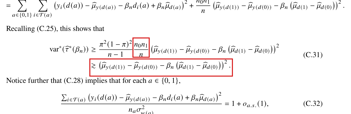
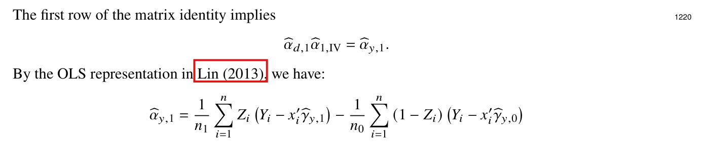
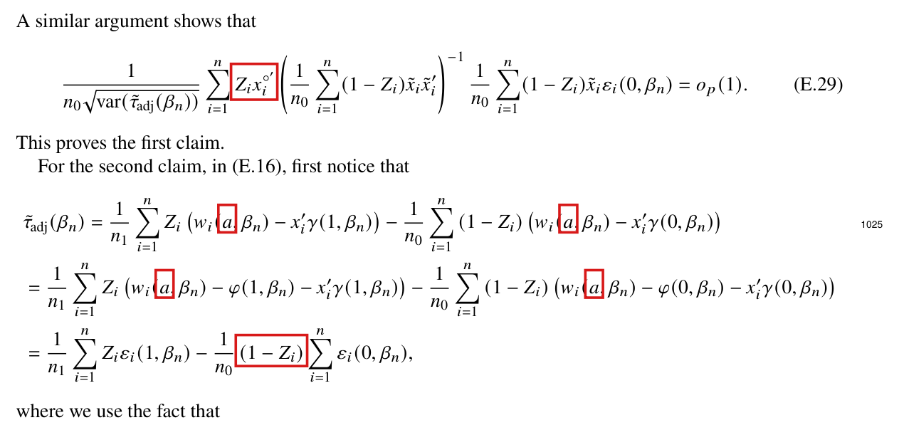
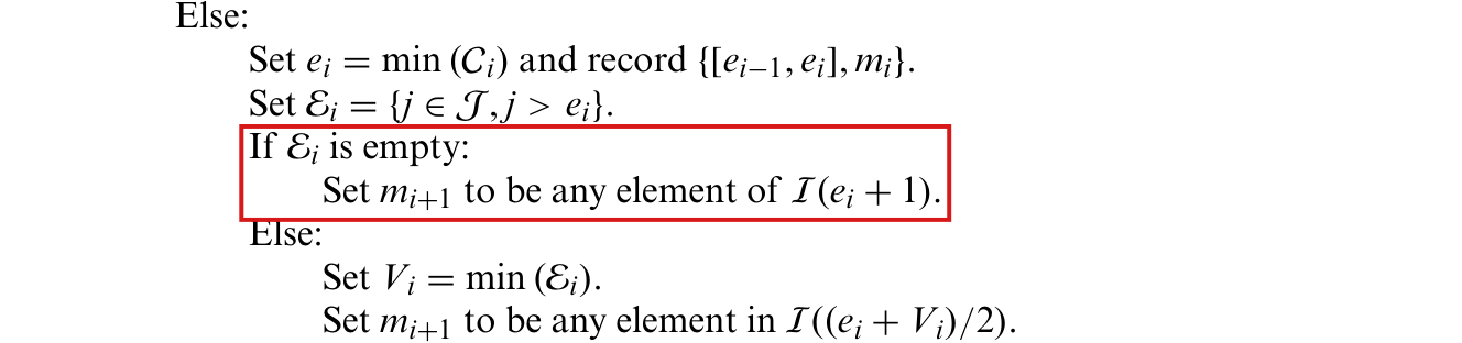
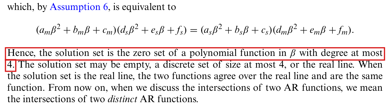
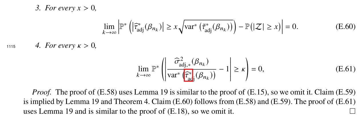
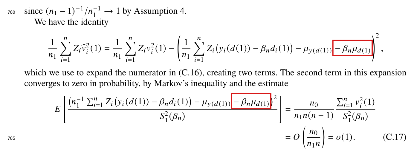
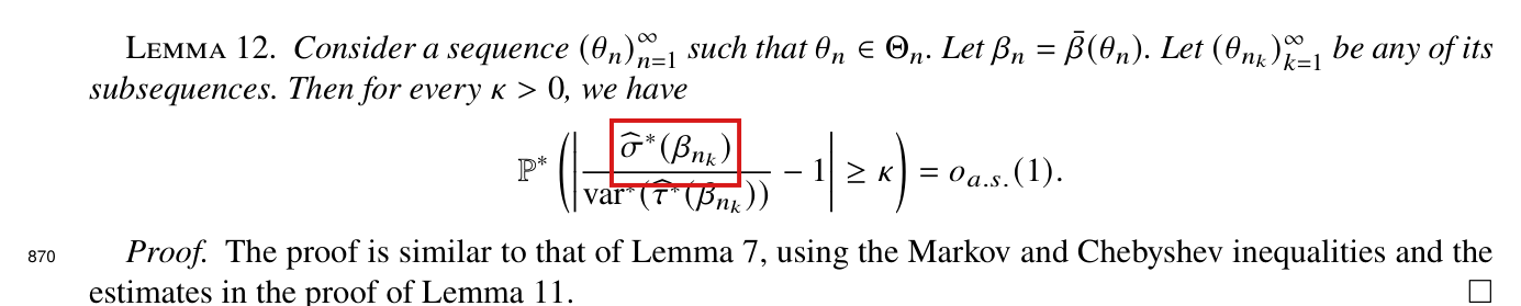
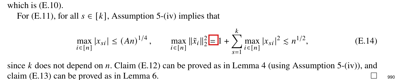
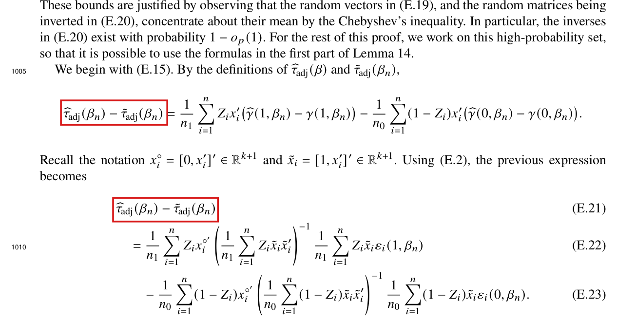
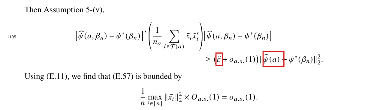
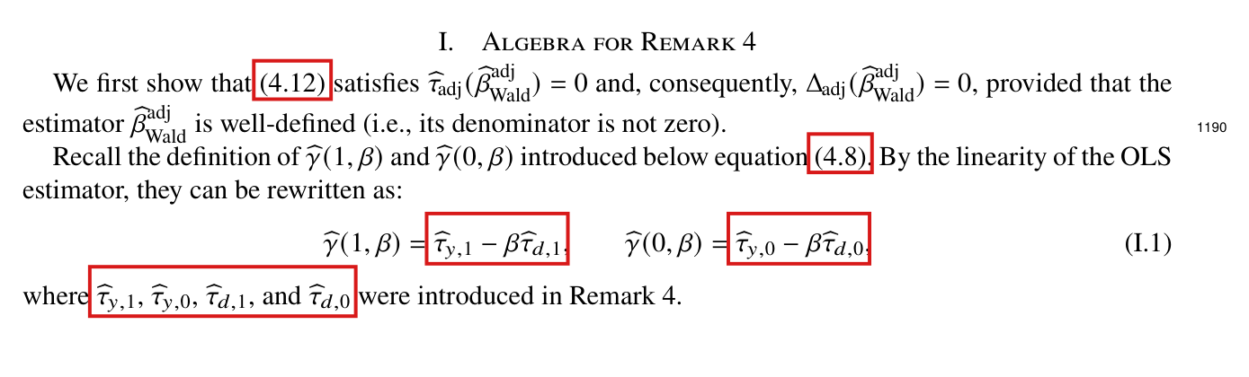
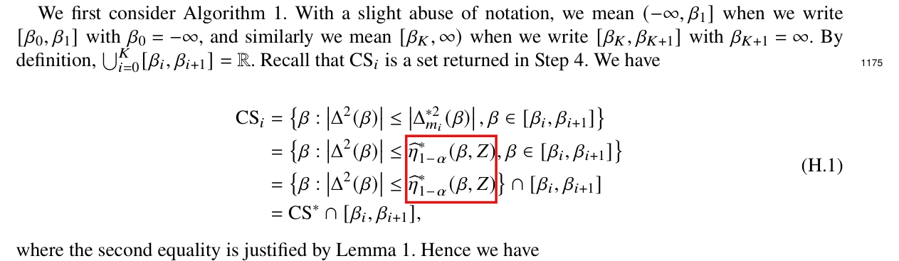
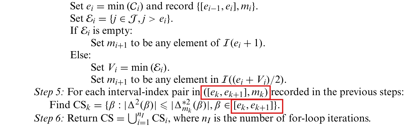
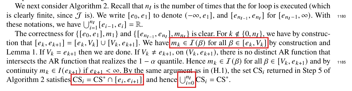
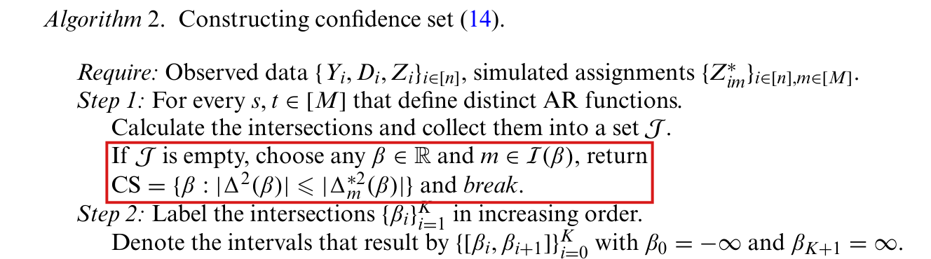
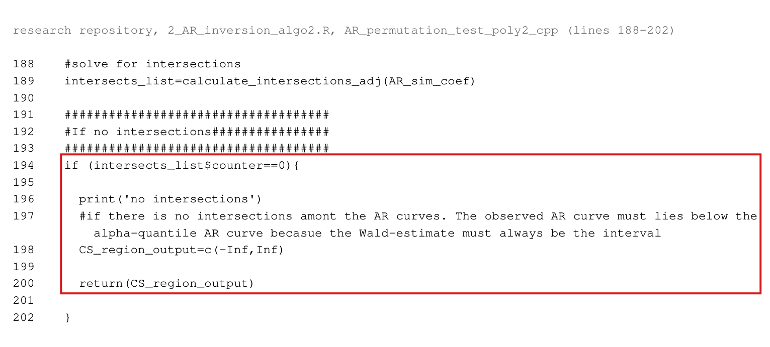
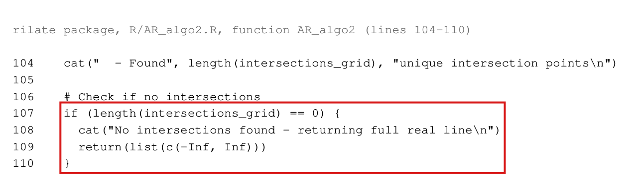
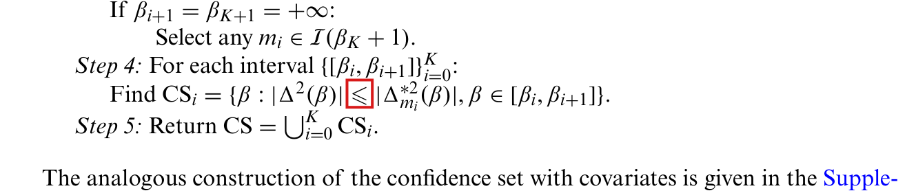
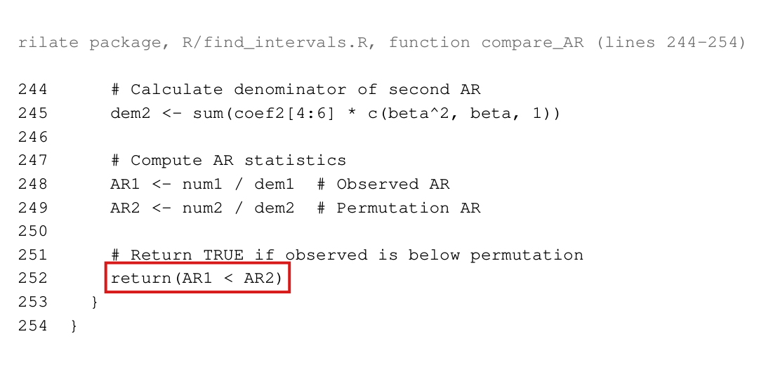
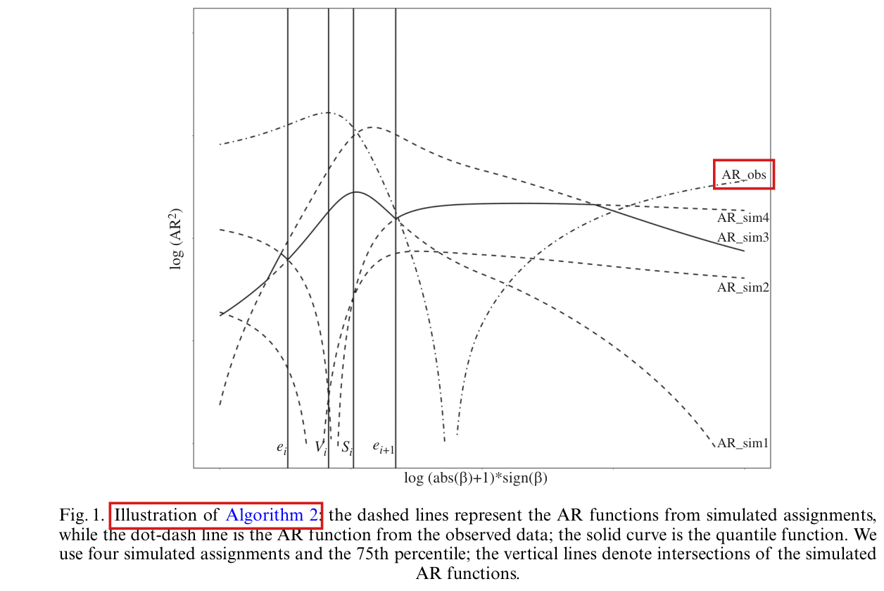
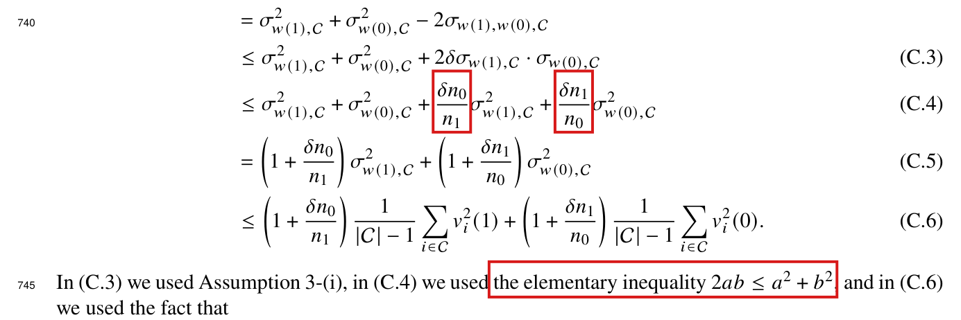
Standing assumptions: [Units, potential outcomes, compliance: main p. 3 (PDF p. 3), Section 2.1] We consider an experiment with $n$ units, where each unit is randomized to treatment or control. Let $y_i(d, z)$ denote the potential outcome of unit $i$ under the potential compliance decision $d \in \{0, 1\}$ and the treatment assignment $z \in \{0, 1\}$. Let $d_i(z)$ denote the compliance decision of the $i$th unit when under treatment status $z$. We write $d_i(1) = 0$ if the $i$th unit is assigned to treatment, but does not receive treatment, and write $d_i(1) = 1$ if it does. The compliance decision $d_i(0)$ under assignment to control is defined analogously. [...] Let $[n] = \{1, \ldots, n\}$. Assumption 1 (Exclusion restriction). For all $i \in [n]$, $y_i(d, z)$ is independent of $z$. This assumption implies that treatment assignment affects outcomes only through treatment receipt, and hence $y_i(d, 1) = y_i(d, 0)$ for all $i \in [n]$. Given this assumption, we write $y_i(d)$ from now on to denote the potential outcome under treatment status $d$. [main p. 4 (PDF p. 4)] Assumption 2 (Monotonicity). For all $i \in [n]$, we have $d_i(1) \ge d_i(0)$. Let $\mathcal{C}$ denote the set of compliers, $\mathcal{C} = \{i \in [n] : d_i(0) = 0,\ d_i(1) = 1\}$. (1) Our inferential target is the LATE in the experimental sample, defined by $\bar\beta = \frac{1}{|\mathcal{C}|}\sum_{i \in \mathcal{C}}\{y_i(1) - y_i(0)\}$. (2) We assume throughout the paper that there is at least one complier ($|\mathcal{C}| \ge 1$) so that the quantity is well-defined. [Design and data: main p. 4, Section 2.2] We assume that the experiments under consideration are completely randomized: among $n$ units, researchers assign $n_1$ units to treatment, chosen uniformly at random. [...] For each unit $i$, we let $Z_i$ be a random variable such that $Z_i = 1$ if unit $i$ is assigned to treatment and $Z_i = 0$ otherwise. By definition, $\mathrm{pr}(Z_i = 1) = n_1/n$, and we introduce the shorthand $\pi = n_1/n$. For each unit $i$, researchers observe compliance decisions $D_i = d_i(Z_i)$ and outcomes $Y_i = y_i(D_i)$. Each unit $i$ may additionally be associated with some covariate information [...]; if so, this information is collected in a column vector $x_i \in \mathbb{R}^k$. Throughout the paper we assume that $k$ does not change with the sample size $n$. [...] We adopt the finite-population (design-based) framework, treating the potential outcomes and compliance decisions as fixed parameters [...]. The sole source of randomness in our model is the vector of random treatment assignments, and statistical uncertainties are evaluated exclusively with respect to this randomness. [Studentized statistic: main pp. 4-5, Section 3.1] For all $\beta \in \mathbb{R}$, we define the statistic $\hat\tau(\beta) = \frac{1}{n}\sum_{i=1}^n (Y_i - \beta D_i)(Z_i - \pi)$. [...] A short calculation shows that $\hat\tau(\beta) = \pi(1-\pi)\left\{\frac{1}{n_1}\sum_{i=1}^n Z_i(Y_i - \beta D_i) - \frac{1}{n_0}\sum_{i=1}^n (1 - Z_i)(Y_i - \beta D_i)\right\}$, where $n_0 = n - n_1$ [...]. We further define $\hat v_i(1, \beta) = Y_i - \beta D_i - \frac{1}{n_1}\sum_{j=1}^n Z_j(Y_j - \beta D_j)$, $\hat v_i(0, \beta) = Y_i - \beta D_i - \frac{1}{n_0}\sum_{j=1}^n (1 - Z_j)(Y_j - \beta D_j)$. (3) Using this notation, we define the variance estimator $\hat\sigma^2(\beta) = \frac{\pi^2(1-\pi)^2}{n_1^2}\sum_{i=1}^n Z_i\hat v_i^2(1, \beta) + \frac{\pi^2(1-\pi)^2}{n_0^2}\sum_{i=1}^n (1 - Z_i)\hat v_i^2(0, \beta)$ and the studentized statistic $\Delta(\beta) = \frac{\hat\tau(\beta)}{\hat\sigma(\beta)}$. (4) We will use the absolute value $|\Delta(\beta)|$ as our test statistic and construct confidence sets by test inversion. We refer to the test statistic $\Delta(\beta)$ in (4) as the AR statistic. [Randomization distribution and confidence set: main pp. 5-6, Section 3.2] The assignment vector $Z = (Z_1, \ldots, Z_n)$ is a random vector in $\{0, 1\}^n$. Let $Z^*$ be a random vector with the same distribution as $Z$ and which is independent of $Z$. We use $\mathbb{P}^*$ to denote the conditional (on $Z$) probability measure induced by $Z^*$. We define $\hat\tau^* : \mathbb{R} \to \mathbb{R}$ by $\hat\tau^*(\beta) = \frac{1}{n}\sum_{i=1}^n (Y_i - \beta D_i)(Z_i^* - \pi)$, where we recall that by definition $Y_i$ and $D_i$ depend only on $Z_i$ and not on $Z_i^*$. We also define the variance estimator $\hat\sigma^{*2}(\beta) = \frac{\pi^2(1-\pi)^2}{n_1^2}\sum_{i=1}^n Z_i^*\left\{Y_i - \beta D_i - \frac{1}{n_1}\sum_{i=1}^n Z_i^*(Y_i - \beta D_i)\right\}^2 + \frac{\pi^2(1-\pi)^2}{n_0^2}\sum_{i=1}^n (1 - Z_i^*)\left\{Y_i - \beta D_i - \frac{1}{n_0}\sum_{i=1}^n (1 - Z_i^*)(Y_i - \beta D_i)\right\}^2$ [the inner sums are the reassigned-arm means; the paper reuses the index $i$] and the studentized statistic $\Delta^*(\beta) = \frac{\hat\tau^*(\beta)}{\hat\sigma^*(\beta)}$. (5) The distribution of $|\Delta^*(\beta)|$ under $\mathbb{P}^*$ is discrete and supported on $[0, \infty]$. For every $\alpha \in (0, 1)$, there exists a smallest (possibly infinite) value $\eta^*_{1-\alpha}(\beta, Z)$ such that $\mathbb{P}^*\{|\Delta^*(\beta)| \le \eta^*_{1-\alpha}(\beta, Z)\} \ge 1 - \alpha$. (6) Our confidence set is defined as $I^*_{1-\alpha}(Z) = \{\beta \in \mathbb{R} : |\Delta(\beta)| \le \eta^*_{1-\alpha}(\beta, Z)\}$. (7) [Assumptions 3 and 4, parameter space $\Theta_n$: main pp. 6-8] Assumption 3 (Parameter space). Let $n \in \mathbb{N}$ and constants $\delta < 1$ and $A > 0$ be given. Set $w_i(1) = y_i\{d_i(1)\} - \bar\beta d_i(1)$, $w_i(0) = y_i\{d_i(0)\} - \bar\beta d_i(0)$. The following conditions on the potential outcomes and compliance decisions hold. (i) For the given $\delta$, $\sigma_{w(1),w(0),\mathcal{C}} \ge -\delta\,\sigma_{w(1),\mathcal{C}}\,\sigma_{w(0),\mathcal{C}}$. Here, $\sigma_{w(1),w(0),\mathcal{C}}$ is the complier-group covariance of adjusted potential outcomes, $\sigma_{w(1),w(0),\mathcal{C}} = \frac{1}{|\mathcal{C}| - 1}\sum_{i \in \mathcal{C}}\{w_i(1) - \mu_{w(1),\mathcal{C}}\}\{w_i(0) - \mu_{w(0),\mathcal{C}}\}$, where $\mu_{w(a),\mathcal{C}} = |\mathcal{C}|^{-1}\sum_{i \in \mathcal{C}} w_i(a)$ for $a \in \{0, 1\}$, and $\sigma^2_{w(1),\mathcal{C}}$ and $\sigma^2_{w(0),\mathcal{C}}$ are the complier-group potential outcome variances, $\sigma^2_{w(a),\mathcal{C}} = \frac{1}{|\mathcal{C}| - 1}\sum_{i \in \mathcal{C}}\{w_i(a) - \mu_{w(a),\mathcal{C}}\}^2$ for $a \in \{0, 1\}$. If $|\mathcal{C}| = 1$, all variances and covariances are defined to be zero. (ii) For each $a \in \{0, 1\}$ and the given $A$, $\left\{\frac{1}{n}\sum_{i=1}^n |w_i(a) - \mu_{w(a)}|^4\right\}^{1/4} \le A\sigma_{w(a)}$, where $\mu_{w(a)} = n^{-1}\sum_{i=1}^n w_i(a)$ and $\sigma^2_{w(a)} = (n-1)^{-1}\sum_{i=1}^n \{w_i(a) - \mu_{w(a)}\}^2$. [...] Assumption 4 (Completely randomized experiment). Given $n \in \mathbb{N}$ and a constant $0 < r \le 1/2$, we have $n_1 \in [rn, (1-r)n]$. We denote the parameter space of potential outcomes, compliance decisions and experimental designs satisfying Assumptions 1-4 with $n$ units and constants $\delta$, $r$ and $A$ by $\Theta_n(\delta, r, A) = \left\{\left(\{(y_i(1), y_i(0), d_i(1), d_i(0))\}_{i=1}^n, \Pi_n\right)\right\}$, where $\{(y_i(1), y_i(0), d_i(1), d_i(0))\}_{i=1}^n$ satisfies Assumption 3 with constants $\delta$ and $A$, and $\Pi_n$ is a distribution of random assignment variables $\{Z_i\}_{i=1}^n$ implementing complete randomization that satisfies Assumption 4 with constant $r$. Each combination of potential outcomes, compliance decisions and an experimental design completely determines the distribution of our test statistic. [...] For each parameter $\theta$ in the parameter space, we denote its LATE by $\bar\beta(\theta)$. [Regression adjustment: main pp. 8-10, Sections 4.1-4.3] [...] each unit $i$ comes equipped with a column vector $x_i \in \mathbb{R}^k$ of covariates for some $k \in \mathbb{N}$. We suppose that each $x_i$ is demeaned, meaning that $\sum_{i=1}^n x_i = 0_k$, where $0_k$ denotes the zero vector in $\mathbb{R}^k$. [...] We denote the $s$th element of $x_i$ by $x_{si}$. Given a $\beta \in \mathbb{R}$ and a treatment assignment vector $Z$, consider the linear regression $Y_i - \beta D_i \sim (1 - Z_i)\varphi_0 + Z_i\varphi_1 + (1 - Z_i)x_i'\gamma_0 + Z_i x_i'\gamma_1$. (8) This is an interacted linear regression that regresses $Y_i - \beta D_i$ on $((1 - Z_i), Z_i, (1 - Z_i)x_i, Z_i x_i)$ without an intercept. For each $\beta$, denote the ordinary least squares (OLS) estimators resulting from (8) by $\hat\varphi(0, \beta)$, $\hat\varphi(1, \beta)$, $\hat\gamma(0, \beta)$ and $\hat\gamma(1, \beta)$, corresponding to the order in which the associated coefficients appear in (8). We define the randomization statistics $\hat\varphi^*(0, \beta)$, $\hat\varphi^*(1, \beta)$, $\hat\gamma^*(0, \beta)$ and $\hat\gamma^*(1, \beta)$ similarly by using $Z^*$ instead of $Z$. [main p. 9] We define the covariate-adjusted difference-in-means statistic as $\hat\tau_{\mathrm{adj}}(\beta) = \frac{1}{n_1}\sum_{i=1}^n Z_i\{Y_i - \beta D_i - x_i'\hat\gamma(1, \beta)\} - \frac{1}{n_0}\sum_{i=1}^n (1 - Z_i)\{Y_i - \beta D_i - x_i'\hat\gamma(0, \beta)\}$, (9) and we define the covariate-adjusted randomization estimator $\hat\tau^*_{\mathrm{adj}}(\beta)$ analogously, again replacing $Z_i$ by $Z_i^*$ and replacing $\hat\gamma(0, \beta)$ and $\hat\gamma(1, \beta)$ by their randomization analogues. [...] The residual estimators associated with (8) and their randomization-based counterparts are $\hat\varepsilon_i(\beta) = Y_i - \beta D_i - \hat\varphi(Z_i, \beta) - x_i'\hat\gamma(Z_i, \beta)$, $\hat\varepsilon_i^*(\beta) = Y_i - \beta D_i - \hat\varphi^*(Z_i^*, \beta) - x_i'\hat\gamma^*(Z_i^*, \beta)$. We use these to define the variance estimators $\hat\sigma^2_{\mathrm{adj}}(\beta) = \frac{1}{n_1^2}\sum_{i=1}^n Z_i\hat\varepsilon_i(\beta)^2 + \frac{1}{n_0^2}\sum_{i=1}^n (1 - Z_i)\hat\varepsilon_i(\beta)^2$, $\hat\sigma^{2*}_{\mathrm{adj}}(\beta) = \frac{1}{n_1^2}\sum_{i=1}^n Z_i^*\hat\varepsilon_i^*(\beta)^2 + \frac{1}{n_0^2}\sum_{i=1}^n (1 - Z_i^*)\hat\varepsilon_i^*(\beta)^2$. The adjusted studentized difference-in-means statistics are then $\Delta_{\mathrm{adj}}(\beta) = \frac{\hat\tau_{\mathrm{adj}}(\beta)}{\hat\sigma_{\mathrm{adj}}(\beta)}$, $\Delta^*_{\mathrm{adj}}(\beta) = \frac{\hat\tau^*_{\mathrm{adj}}(\beta)}{\hat\sigma^*_{\mathrm{adj}}(\beta)}$. (10) [...] Given $\alpha \in (0, 1)$, there exists a smallest (possibly infinite) value $\eta^{\mathrm{adj},*}_{1-\alpha}(\beta, Z)$ such that $\mathbb{P}^*\{|\Delta^*_{\mathrm{adj}}(\beta)| \le \eta^{\mathrm{adj},*}_{1-\alpha}(\beta, Z)\} \ge 1 - \alpha$. [main p. 10] Our proposed confidence set is $I^{\mathrm{adj},*}_{1-\alpha}(Z) = \{\beta \in \mathbb{R} : |\Delta_{\mathrm{adj}}(\beta)| \le \eta^{\mathrm{adj},*}_{1-\alpha}(\beta, Z)\}$. (11) [Assumption 5 and parameter space $\Xi_n$: main pp. 10-11] Assumption 5. Let $k, n \in \mathbb{N}$ and constants $\delta < 1$ and $\tilde\varepsilon, A, B > 0$ be given. For each $a \in \{0, 1\}$, define $\varepsilon_i(a, \bar\beta) = y_i\{d_i(a)\} - \bar\beta d_i(a) - \varphi(a, \bar\beta) - x_i'\gamma(a, \bar\beta)$. The following conditions on the potential outcomes, compliance decisions and covariates hold. (i) For the given $\delta$, $\sigma_{\varepsilon(1,\bar\beta),\varepsilon(0,\bar\beta)} \ge -\delta\sigma_{\varepsilon(1,\bar\beta)}\sigma_{\varepsilon(0,\bar\beta)}$. (ii) For each $a \in \{0, 1\}$ and the given $B$, $\left\{\frac{1}{n}\sum_{i=1}^n \varepsilon_i^4(a, \bar\beta)\right\}^{1/4} \le B\sigma_{\varepsilon(a,\bar\beta)}$. (iii) We have that $\sum_{i=1}^n x_i = 0_k$. (iv) For all $s \in [k]$ and the given $A$, we have that $n^{-1}\sum_{i=1}^n x_{si}^4 \le A$. (v) Let $\lambda_{\min}$ denote the smallest eigenvalue of $n^{-1}\sum_{i=1}^n x_i x_i'$. Then for the given $\tilde\varepsilon$, $\lambda_{\min} \ge \tilde\varepsilon$. We denote the parameter space of potential outcomes, compliance decisions, covariates and experimental designs satisfying Assumptions 1, 2, 4 and 5 with $n$ units, covariates of dimension $k$, and constants $\delta$, $\tilde\varepsilon$, $A$, $B$ and $r$ by $\Xi_n(k, \delta, \tilde\varepsilon, A, B, r) = \left\{\left(\{(y_i(1), y_i(0), d_i(1), d_i(0), x_i)\}_{i=1}^n, \Pi_n\right)\right\}$. Here, $\{(y_i(1), y_i(0), d_i(1), d_i(0), x_i)\}_{i=1}^n$ satisfies Assumption 5 with constants $\delta$, $\tilde\varepsilon$, $A$ and $B$, and $\Pi_n$ is a distribution of random assignment variables $\{Z_i\}_{i=1}^n$ implementing complete randomization that satisfies Assumption 4 with constant $r$. [The population variances and covariance in Assumption 5 are those of Supplement A.1 below, with divisor $n - 1$; $\varphi(a, \beta)$, $\gamma(a, \beta)$ are defined in Supplement D.2 below.] [Supplement A, notation: Supplement p. 21 (Supplement PDF p. 1)] We let $\mathbb{N}$ denote the positive integers [...]. We use the notation $\lesssim$ to denote inequalities that hold up to a constant independent of $n$. [...] We also define a set $\mathcal{A}$ of always-takers and a set $\mathcal{N}$ of never-takers by $\mathcal{A} = \{i \in [n] : d_i(0) = 1, d_i(1) = 1\}$, $\mathcal{N} = \{i \in [n] : d_i(0) = 0, d_i(1) = 0\}$. Let $\mathcal{T}(1), \mathcal{T}(0) \subset [n]$ denote the sets of subjects in the treatment and control groups defined by $Z$, respectively, so that $\mathcal{T}(1) = \{i \in [n] : Z_i = 1\}$, $\mathcal{T}(0) = \{i \in [n] : Z_i = 0\}$. Given a vector $v$, we use $\|v\|_2$ to denote the standard $l_2$ vector norm. [...] A.1. For any vector $q = (q_i)_{i=1}^n \in \mathbb{R}^n$, we define the population mean and variance by $\mu_q = \frac{1}{n}\sum_{i=1}^n q_i$, $\sigma_q^2 = \frac{1}{n-1}\sum_{i=1}^n (q_i - \mu_q)^2$. We also define within-group variances for each group $G \in \{\mathcal{A}, \mathcal{C}, \mathcal{N}\}$ by $\sigma^2_{q,G} = \frac{1}{|G| - 1}\sum_{i \in G}(q_i - \mu_{q,G})^2$, where $\mu_{q,G} = \frac{1}{|G|}\sum_{i \in G} q_i$ if $|G| \ge 2$ and zero otherwise. Given an additional vector $\tilde q = (\tilde q_i)_{i=1}^n \in \mathbb{R}^n$, we define the population covariance by $\sigma_{q\tilde q} = \frac{1}{n-1}\sum_{i=1}^n (q_i - \mu_q)(\tilde q_i - \mu_{\tilde q})$, and the within-group covariances by $\sigma_{q\tilde q,G} = \frac{1}{|G| - 1}\sum_{i \in G}(q_i - \mu_{q,G})(\tilde q_i - \mu_{\tilde q,G})$, if $|G| \ge 2$ and zero otherwise. A.2. Let $\mathcal{Z}$ be a mean zero, variance one normal random variable. [...] For an $\alpha \in (0, 1)$, define $z_{1-\alpha} \in \mathbb{R}$ as the value such that $\mathbb{P}(\mathcal{Z} > z_{1-\alpha}) = \alpha$. [Supplement B.1 and B.3: Supplement p. 22 (PDF p. 2)] Lemma 2. For all $\beta \in \mathbb{R}$, the variance of $\hat\tau(\beta)$ is $\operatorname{var}(\hat\tau(\beta)) = \frac{S_1^2(\beta)}{n_1} + \frac{S_0^2(\beta)}{n_0} - \frac{S_{10}^2(\beta)}{n}$, (B.1) where $S_1^2(\beta) = \frac{\pi^2(1-\pi)^2}{n-1}\sum_{i=1}^n v_i(1, \beta)^2$, $S_0^2(\beta) = \frac{\pi^2(1-\pi)^2}{n-1}\sum_{i=1}^n v_i(0, \beta)^2$, $S_{10}^2(\beta) = \frac{\pi^2(1-\pi)^2}{n-1}\sum_{i=1}^n (v_i(1, \beta) - v_i(0, \beta))^2$, (B.2) $v_i(1, \beta) = y_i(d_i(1)) - \beta d_i(1) - \frac{1}{n}\sum_{i=1}^n (y_i(d_i(1)) - \beta d_i(1))$, (B.3) $v_i(0, \beta) = y_i(d_i(0)) - \beta d_i(0) - \frac{1}{n}\sum_{i=1}^n (y_i(d_i(0)) - \beta d_i(0))$. (B.4) [...] Lemma 3. We have $E[\hat\tau(\beta)] = 0$ when $\beta = |\mathcal{C}|^{-1}\sum_{i \in \mathcal{C}}(y_i(1) - y_i(0))$. [Supplement C, conventions: Supplement p. 23 (PDF p. 3)] Throughout this section, we let $\delta, r, A$ be the constants fixed in the statement of Theorem 1, and set $\Theta_n = \Theta_n(\delta, r, A)$. The notation $\Theta_n$ encodes Assumptions 1-4. We typically denote elements of $\Theta_n$ by $\theta_n$. For each model $\theta_n$, we denote its local average treatment effect by $\bar\beta(\theta_n)$ [...]. In various lemmas below, we will consider subsequences $(\theta_{n_k})_{k=1}^\infty$ of a given sequence $(\theta_n)_{n=1}^\infty$ of models. We let $n_{1k}$ denote the number of elements in the treatment group of $\theta_{n_k}$, and $n_{0k}$ the number of elements in the control group of $\theta_{n_k}$, so that $n_{0k} + n_{1k} = n_k$. [...] For the remainder of the proofs, we will implicitly assume that the variances $\sigma^2_{w(a)}$, for $a \in \{0, 1\}$ as defined in Assumption 3, are both strictly positive. This entails no loss of generality provided we adopt the convention that $0/0 = 0$. If both variances are zero, then the complier treatment effect is constant and additive, so the exact coverage result of the randomization-based CI in Imbens & Rosenbaum (2005) applies. [...] Similar comments apply to the proofs in Section D. [...] In results on sequences $(\theta_n)_{n=1}^\infty$, we will generally omit the $n$-dependence on $w_i(1)$, $w_i(0)$, and other model-dependent quantities for brevity. [Supplement C.3: Supplement pp. 27-28 (PDF pp. 7-8)] We write $E^*$ and $\operatorname{var}^*$ for expectation and variance under the probability measure $\mathbb{P}^*$. By Lemma 3, for any $\beta$ we have $E^*[\hat\tau^*(\beta)] = 0$, and by Lemma 2, $\operatorname{var}^*(\hat\tau^*(\beta)) = \frac{S_1^{*2}(\beta)}{n_1} + \frac{S_0^{*2}(\beta)}{n_0}$, (C.25) where $S_1^{*2}(\beta) = S_0^{*2}(\beta) = \frac{\pi^2(1-\pi)^2}{n-1}\sum_{i=1}^n \left(Y_i - \beta D_i - \frac{1}{n}\sum_{i=1}^n (Y_i - \beta D_i)\right)^2$. (C.26) [...] We recall that $\mu_Y = \frac{1}{n}\sum_{i=1}^n Y_i$, $\mu_D = \frac{1}{n}\sum_{i=1}^n D_i$ and define $\hat\mu_{y(d(a))} = \frac{1}{n_a}\sum_{i \in \mathcal{T}(a)} y_i(d_i(a))$, $\hat\mu_{d(a)} = \frac{1}{n_a}\sum_{i \in \mathcal{T}(a)} d_i(a)$, for each $a \in \{0, 1\}$. [Supplement D, least-squares parameters and infeasible estimator: Supplement pp. 31-32 (PDF pp. 11-12)] We let $k, \delta, \tilde\varepsilon, A, B, r$ be the constants fixed in the statement of Theorem 2, and set $\Xi_n = \Xi_n(k, \delta, \tilde\varepsilon, A, B, r)$. D.2. Suppose a $\beta \in \mathbb{R}$ is given. Then we define, for each $a \in \{0, 1\}$, outcomes $w_i(a, \beta)$ by $w_i(a, \beta) = y_i(d_i(a)) - \beta d_i(a)$. (D.1) We define the least-squares regression parameters $\varphi(a, \beta) : \{0, 1\} \times \mathbb{R} \to \mathbb{R}$, $\gamma(a, \beta) : \{0, 1\} \times \mathbb{R} \to \mathbb{R}^k$, by $(\varphi(a, \beta), \gamma(a, \beta)) = \arg\min_{(s,t) \in \mathbb{R} \times \mathbb{R}^k}\frac{1}{n}\sum_{i=1}^n (w_i(a, \beta) - s - x_i't)^2$, (D.2) where we interpret $t$ as a column vector. We define the residuals for (D.2) by $\varepsilon_i(a, \beta) = w_i(a, \beta) - \varphi(a, \beta) - x_i'\gamma(a, \beta)$. The parameters $\varphi^*(a, \beta)$ and $\gamma^*(a, \beta)$ are defined similarly, by replacing $w_i(a, \beta)$ with $Y_i - \beta D_i$ in (D.2), and we define the associated residuals $\varepsilon_i^*(\beta)$ by $\varepsilon_i^*(\beta) = Y_i - \beta D_i - \varphi^*(a, \beta) - x_i'\gamma^*(a, \beta)$. (D.3) These definitions imply that $\varphi^*(0, \beta) = \varphi^*(1, \beta)$ and $\gamma^*(0, \beta) = \gamma^*(1, \beta)$. D.3. To analyze the asymptotic behavior of $\hat\tau_{\mathrm{adj}}(\beta)$, we define the infeasible estimator $\tilde\tau_{\mathrm{adj}}(\beta) = \frac{1}{n_1}\sum_{i=1}^n Z_i(Y_i - \beta D_i - x_i'\gamma(1, \beta)) - \frac{1}{n_0}\sum_{i=1}^n (1 - Z_i)(Y_i - \beta D_i - x_i'\gamma(0, \beta))$. (D.4) The infeasible estimator $\tilde\tau^*_{\mathrm{adj}}(\beta)$ is defined similarly, replacing $Z_i$ by $Z_i^*$, and $\gamma(1, \beta)$ and $\gamma(0, \beta)$ by $\gamma^*(1, \beta)$ and $\gamma^*(0, \beta)$, respectively. A straightforward adaptation of Lemma 2 shows that $\operatorname{var}(\tilde\tau_{\mathrm{adj}}(\beta)) = \frac{\mathcal{S}_1^2(\beta)}{n_1} + \frac{\mathcal{S}_0^2(\beta)}{n_0} - \frac{\mathcal{S}_{10}^2(\beta)}{n}$, (D.5) where $\mathcal{S}_1^2(\beta) = \frac{1}{n-1}\sum_{i=1}^n \varepsilon_i^2(1, \beta)$, $\mathcal{S}_0^2(\beta) = \frac{1}{n-1}\sum_{i=1}^n \varepsilon_i^2(0, \beta)$, $\mathcal{S}_{10}^2(\beta) = \frac{1}{n-1}\sum_{i=1}^n (\varepsilon_i(1, \beta) - \varepsilon_i(0, \beta))^2$. Similarly, $\operatorname{var}^*(\tilde\tau^*_{\mathrm{adj}}(\beta)) = \frac{\mathcal{S}_{1,*}^2(\beta)}{n_1} + \frac{\mathcal{S}_{0,*}^2(\beta)}{n_0}$, $\mathcal{S}_{1,*}^2(\beta) = \mathcal{S}_{0,*}^2(\beta) = \frac{1}{n-1}\sum_{i=1}^n \varepsilon_i^*(\beta)^2$. (D.6) [Supplement E.1: Supplement p. 32 (PDF p. 12)] Denote $x_i^\circ = [0, x_i']' \in \mathbb{R}^{k+1}$ and $\tilde x_i = [1, x_i']' \in \mathbb{R}^{k+1}$. For $a \in \{0, 1\}$, define $\psi(a, \beta) = \begin{bmatrix}\varphi(a, \beta) \\ \gamma(a, \beta)\end{bmatrix}$, $\hat\psi(a, \beta) = \begin{bmatrix}\hat\varphi(a, \beta) \\ \hat\gamma(a, \beta)\end{bmatrix}$. (E.1) We denote their randomization counterparts as $\psi^*(a, \beta)$ and $\hat\psi^*(a, \beta)$. Lemma 14. The following claims hold. 1. We have $\hat\psi(1, \beta) - \psi(1, \beta) = \left(\frac{1}{n_1}\sum_{i=1}^n Z_i\tilde x_i\tilde x_i'\right)^{-1}\frac{1}{n_1}\sum_{i=1}^n Z_i\tilde x_i\varepsilon_i(1, \beta)$ (E.2) and $\hat\psi(0, \beta) - \psi(0, \beta) = \left(\frac{1}{n_0}\sum_{i=1}^n (1 - Z_i)\tilde x_i\tilde x_i'\right)^{-1}\frac{1}{n_0}\sum_{i=1}^n (1 - Z_i)\tilde x_i\varepsilon_i(0, \beta)$, (E.3) provided that the matrices $\sum_{i=1}^n Z_i\tilde x_i\tilde x_i'$ and $\sum_{i=1}^n (1 - Z_i)\tilde x_i\tilde x_i'$ are invertible. 2. For each $a \in \{0, 1\}$, $\sum_{i=1}^n \tilde x_i\varepsilon_i(a, \beta) = 0_{k+1}$. (E.4) [Monte Carlo confidence set, AR functions, index set: main pp. 12-14, Sections 5.1-5.3] Let $M$ be the number of simulated assignments, and let $\Delta_m^*(\beta)$ be the AR statistic associated with the $m$th assignment. We define $\hat\eta^*_{1-\alpha}(\beta, Z) = \min\left\{|\Delta_s^*(\beta)| : \frac{1}{M}\sum_{m=1}^M \mathbf{1}\{|\Delta_m^*(\beta)| \le |\Delta_s^*(\beta)|\} \ge 1 - \alpha\right\}$ (13) and define the confidence set of interest as $\hat I^*_{1-\alpha}(Z) = \{\beta \in \mathbb{R} : |\Delta(\beta)| \le \hat\eta^*_{1-\alpha}(\beta, Z)\}$. (14) [Section 5.2] For the observed AR function, we have $\Delta^2(\beta) = \frac{a\beta^2 + b\beta + c}{d\beta^2 + e\beta + f}$, (15) where $a = \left\{\frac{1}{n}\sum_{i=1}^n D_i(Z_i - \pi)\right\}^2$, $b = -2\left\{\frac{1}{n}\sum_{i=1}^n Y_i(Z_i - \pi)\right\}\left\{\frac{1}{n}\sum_{i=1}^n D_i(Z_i - \pi)\right\}$, $c = \left\{\frac{1}{n}\sum_{i=1}^n Y_i(Z_i - \pi)\right\}^2$, $d = \frac{\pi^2(1-\pi)^2}{n_1^2}\sum_{i=1}^n Z_i\left(D_i - \frac{1}{n_1}\sum_{j=1}^n Z_j D_j\right)^2 + \frac{\pi^2(1-\pi)^2}{n_0^2}\sum_{i=1}^n (1 - Z_i)\left\{D_i - \frac{1}{n_0}\sum_{j=1}^n (1 - Z_j)D_j\right\}^2$, $e = -2\frac{\pi^2(1-\pi)^2}{n_1^2}\sum_{i=1}^n Z_i\left(Y_i - \frac{1}{n_1}\sum_{j=1}^n Z_j Y_j\right)\left(D_i - \frac{1}{n_1}\sum_{j=1}^n Z_j D_j\right) - 2\frac{\pi^2(1-\pi)^2}{n_0^2}\sum_{i=1}^n (1 - Z_i)\left\{Y_i - \frac{1}{n_0}\sum_{j=1}^n (1 - Z_j)Y_j\right\}\left\{D_i - \frac{1}{n_0}\sum_{j=1}^n (1 - Z_j)D_j\right\}$, $f = \frac{\pi^2(1-\pi)^2}{n_1^2}\sum_{i=1}^n Z_i\left(Y_i - \frac{1}{n_1}\sum_{j=1}^n Z_j Y_j\right)^2 + \frac{\pi^2(1-\pi)^2}{n_0^2}\sum_{i=1}^n (1 - Z_i)\left\{Y_i - \frac{1}{n_0}\sum_{j=1}^n (1 - Z_j)Y_j\right\}^2$. [main p. 13] We denote the $m$th simulated assignment by $Z_m^*$ and its $i$th entry by $Z_{im}^*$. For the AR function calculated from the $m$th simulated assignment, we have $\Delta_m^{*2}(\beta) = \frac{a_m\beta^2 + b_m\beta + c_m}{d_m\beta^2 + e_m\beta + f_m}$, (16) where the coefficients are calculated using the same formulas as above, but with the $Z_i$ replaced by the simulated assignments $Z_{im}^*$. [main p. 14] Assumption 6. Let $d\beta^2 + e\beta + f$ and $d_m\beta^2 + e_m\beta + f_m$ be as defined in (15) and (16), respectively. As functions of $\beta$, they are positive everywhere on $\mathbb{R}$. Remark 7. [...] The intersections of two AR functions are solutions to the equality $\Delta_m^{*2}(\beta) = \Delta_s^{*2}(\beta)$, where $m$ and $s$ are two indices for simulated assignments. [...] Hence, the solution set is the zero set of a polynomial function in $\beta$ with degree at most 4. The solution set may be empty, a discrete set of size at most 4, or the real line. When the solution set is the real line, the two functions agree over the real line and are the same function. From now on, when we discuss the intersections of two AR functions, we mean the intersections of two distinct AR functions. [Section 5.3] For every $\beta \in \mathbb{R}$, let $\mathcal{I}(\beta)$ be the set of indices of randomizations that attain equality in the definition of $\hat\eta^*_{1-\alpha}(\beta, Z)$; that is, $\mathcal{I}(\beta) = \{m : |\Delta_m^*(\beta)| = \hat\eta^*_{1-\alpha}(\beta, Z)\}$. (17) The set is always nonempty, by (13).
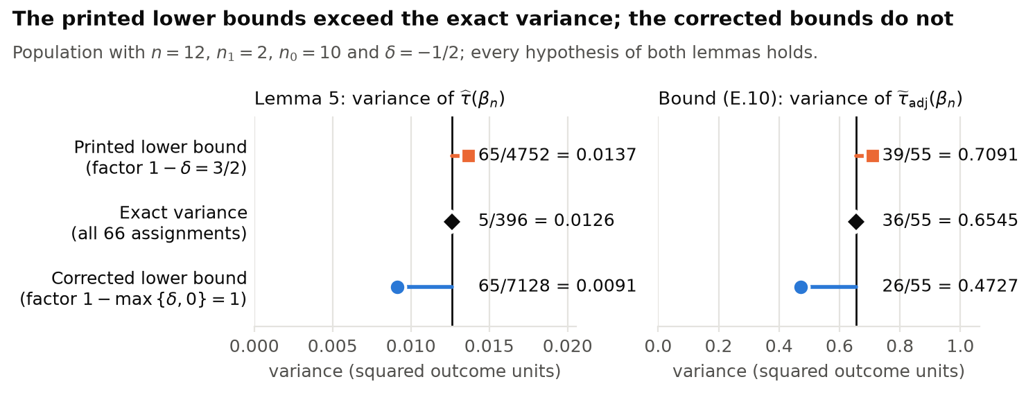
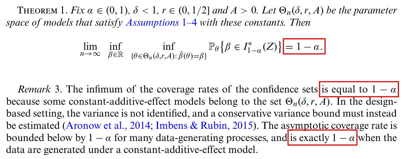
Effective claim (source TeX): [Printed statements refuted: main p. 8 (PDF p. 8)] Theorem 1. Fix $\alpha \in (0, 1)$, $\delta < 1$, $r \in (0, 1/2]$ and $A > 0$. Let $\Theta_n(\delta, r, A)$ be the parameter space of models that satisfy Assumptions 1-4 with these constants. Then $\lim_{n\to\infty}\inf_{\beta\in\mathbb{R}}\inf_{\{\theta\in\Theta_n(\delta,r,A):\,\bar\beta(\theta)=\beta\}}\mathbb{P}_\theta\{\beta \in I^*_{1-\alpha}(Z)\} = 1 - \alpha$. Remark 3. The infimum of the coverage rates of the confidence sets is equal to $1 - \alpha$ because some constant-additive-effect models belong to the set $\Theta_n(\delta, r, A)$. In the design-based setting, the variance is not identified, and a conservative variance bound must instead be estimated (Aronow et al., 2014; Imbens & Rubin, 2015). The asymptotic coverage rate is bounded below by $1 - \alpha$ for many data-generating processes, and is exactly $1 - \alpha$ when the data are generated under a constant-additive-effect model. [main p. 11 (PDF p. 11)] Theorem 2. Fix $k \in \mathbb{N}$, $\alpha \in (0, 1)$, $r \in (0, 1/2]$, $\delta < 1$ and $\tilde\varepsilon, A, B > 0$. Let $\Xi_n(k, \delta, \tilde\varepsilon, A, B, r)$ be the parameter space of models that satisfy Assumptions 1, 2, 4 and 5 with these constants. Then $\lim_{n\to\infty}\inf_{\beta\in\mathbb{R}}\inf_{\{\theta\in\Xi_n(k,\delta,\tilde\varepsilon,A,B,r):\,\bar\beta(\theta)=\beta\}}\mathbb{P}_\theta\{\beta \in I^{\mathrm{adj},*}_{1-\alpha}(Z)\} = 1 - \alpha$. [Printed proof step refuted: Supplement p. 31 (PDF p. 11)] Finally, note that a sequence of constant-additive-effect models belongs to our parameter set. Hence the inequality holds as an equality. [Counterexample, from the validators; the convention $0/0 = 0$ of Supplement p. 23 is used.] (a) [Moment collapse.] Let $n \ge 2$ and $v_1, \ldots, v_n \in \mathbb{R}$. If $\left\{\frac1n\sum_{i=1}^n v_i^4\right\}^{1/4} \le \frac12\left\{\frac{1}{n-1}\sum_{i=1}^n v_i^2\right\}^{1/2}$, then $v_i = 0$ for all $i$. [Because $\left(\sum_i v_i^2\right)^2 \le n\sum_i v_i^4$ and the hypothesis gives $16(n-1)^2\sum_i v_i^4 \le n\left(\sum_i v_i^2\right)^2$, so that $\{16(n-1)^2 - n^2\}\left(\sum_i v_i^2\right)^2 \le 0$, with $16(n-1)^2 - n^2 = 15(n-2)^2 + 28(n-2) + 12 > 0$.] (b) [Theorem 1 fails for $(\delta, r, A) = (0, 1/4, 1/2)$.] Let $n \ge 2$ and let $\theta$ be any model in $\Theta_n(0, 1/4, 1/2)$, with $\beta = \bar\beta(\theta)$. By (a) applied to $v_i = w_i(a) - \mu_{w(a)}$ and Assumption 3(ii) with $A = 1/2$, $w_i(a) = c_a$ for all $i$, for each $a \in \{0, 1\}$; and $c_1 = c_0$, because $n(c_1 - c_0) = \sum_{i=1}^n \{w_i(1) - w_i(0)\} = \sum_{i \in \mathcal{C}}\{y_i(1) - y_i(0) - \beta\} = 0$. Hence for every assignment $Y_i - \beta D_i = c$ for all $i$, $\hat\tau(\beta) = 0$, $\hat\sigma^2(\beta) = 0$ and $\Delta(\beta) = 0/0 = 0$; likewise $\Delta^*(\beta) = 0$ for every $Z^*$, so $\eta^*_{1-\alpha}(\beta, Z) = 0$ and $\beta \in I^*_{1-\alpha}(Z)$. So $\mathbb{P}_\theta\{\beta \in I^*_{1-\alpha}(Z)\} = 1$ for every model in the class. The class is non-empty for every $n \ge 2$ and every $\beta \in \mathbb{R}$: take all units compliers, $d_i(0) = 0$, $d_i(1) = 1$, $y_i(0) = 0$, $y_i(1) = \beta$, and $n_1 = \lfloor n/2 \rfloor$ (then $w_i(1) = w_i(0) = 0$, Assumption 3(i) reads $0 \ge 0$, 3(ii) reads $0 \le 0$, and $n/4 \le \lfloor n/2 \rfloor \le 3n/4$). Therefore $\inf_{\beta\in\mathbb{R}}\inf_{\{\theta\in\Theta_n(0,1/4,1/2):\,\bar\beta(\theta)=\beta\}}\mathbb{P}_\theta\{\beta \in I^*_{1-\alpha}(Z)\} = 1$ for every $n \ge 2$ and every $\alpha \in (0, 1)$; the limit is $1 \ne 1 - \alpha$. The models exhibited have constant additive effects, so the last sentence of Remark 3 and the last step of the proof of Theorem 1 fail for this class as well. (c) [Theorem 2 fails for $(k, \delta, \tilde\varepsilon, A, B, r) = (1, 0, 1/4, 4, 1/2, 1/4)$.] Let $n \ge 2$ and let $\theta$ be any model in $\Xi_n(1, 0, 1/4, 4, 1/2, 1/4)$, with $\beta = \bar\beta(\theta)$. The population residuals $\varepsilon_i(a, \beta)$ have mean zero, so by (a) and Assumption 5(ii) with $B = 1/2$, $\varepsilon_i(a, \beta) = 0$ for all $i$ and $a$: $w_i(a, \beta) = \varphi(a, \beta) + \gamma(a, \beta)x_i$, and $\varphi(1, \beta) = \varphi(0, \beta)$. On the event that, in each arm, the observed covariate values are not all equal (so that both arm regressions of (8) have full column rank), the fitted coefficients equal $(\varphi(a, \beta), \gamma(a, \beta))$, all fitted residuals are zero, $\hat\tau_{\mathrm{adj}}(\beta) = 0$ and $\Delta_{\mathrm{adj}}(\beta) = 0 \le \eta^{\mathrm{adj},*}_{1-\alpha}(\beta, Z)$, so $\beta \in I^{\mathrm{adj},*}_{1-\alpha}(Z)$. With $Q = n^{-1}\sum_i x_i^2 \ge 1/4$ and $n^{-1}\sum_i x_i^4 \le 4$, the probability that a given arm (of size $m \in [n/4, 3n/4]$) fails to have full column rank is at most $258\,\frac{n - m}{m(n-1)} \le \frac{774}{n-1}$ (Chebyshev's inequality for the arm means of $x_i$ and $x_i^2$ under simple random sampling), so the probability that either arm fails is at most $1548/(n-1)$, uniformly over the class. Hence $\mathbb{P}_\theta\{\beta \in I^{\mathrm{adj},*}_{1-\alpha}(Z)\} \ge \max\{0, 1 - 1548/(n-1)\}$ for every model in the class, whatever is decided for rank-deficient arms. The class is non-empty for every $n \ge 2$ and every $\beta \in \mathbb{R}$: all units compliers, $y_i(0) = 0$, $y_i(1) = \beta$, $n_1 = \lfloor n/2 \rfloor$ and $x_i = (2i - n - 1)/n$, for which $\sum_i x_i = 0$, $n^{-1}\sum_i x_i^2 = \frac{n^2 - 1}{3n^2} \ge \frac14$ and $n^{-1}\sum_i x_i^4 < 1$. Therefore the nested infimum of Theorem 2 at these constants lies in $[\max\{0, 1 - 1548/(n-1)\}, 1]$ and tends to $1 \ne 1 - \alpha$, for every $\alpha \in (0, 1)$. (d) [Exact finite illustration of (c), from the validator.] $n = 6$, $x_i = (2i - 7)/6$, all units compliers, $\beta = 7/3$, $y_i(0) = x_i$, $y_i(1) = \beta + 2x_i$, $n_1 = 3$: the model is in $\Xi_6(1, 0, 1/4, 4, 1/2, 1/4)$ with $\bar\beta = 7/3$ and heterogeneous effects; for each of the 20 assignments $\Delta_{\mathrm{adj}}(\beta) = 0$ and $\beta \in I^{\mathrm{adj},*}_{1-\alpha}(Z)$, although 312 of the 400 values of $\Delta^{*2}_{\mathrm{adj}}(\beta)$ over pairs $(Z, Z^*)$ are non-zero.
: SAP.P002a.T4WholeStatement
Theorem: SAP.P002a.T4
Statement hash: b94f688cafa5280d54bacbce64fe6876e256a76561b1dc7923e4560a69af2f78
Statement definition: SAP.P002a.T4WholeStatement
Certificate. 20261104T193351Z
Declaration review: faithful; 2026-11-04T19:17:43Z; binding v2
Evidence scope: Certification checks formal proof objects. Statement fidelity is a model judgment. Author review is separate.
Proof dependencies: Independently extracted
Manifest annotation reconciliation: Effective use follows the source-bound dependency observation; original annotations are retained in the crosswalk.
AronowAudit.P002.collapse_moments: observed used
AronowAudit.P002.degenerate_model_admissible: observed used
AronowAudit.P002.fourth_moment_CS: observed used
AronowAudit.P002.observedW_constant: observed used
AronowAudit.P002.rawTau_constant: observed used
AronowAudit.P002.theta_half_moment_coverage: observed used
Source and evidence metadata · sap-2026-11-08-assured-release














![Crop of Theorem 1. A red box marks 'delta less than 1' in the list of constants 'Fix alpha in (0,1), delta less than 1, r in (0, 1/2] and A greater than 0'.](exhibits/P002-E002-d.png)