Assumptions and verification
Claim revision: catalog:b567ea3a053e06a585facf03ba8b486d87d4fa3d918963e21feb0b8a1ec07eec
Standing assumptions: Finite-population, design-based setting: the $n$ subjects and their binary potential outcomes are fixed and the only randomness is the complete randomization of $m$ subjects to treatment (plus, where stated, independent Monte Carlo draws and, in Section 6, a missingness vector). Printed and PDF page numbers coincide (Journal of Econometrics 251 (2025) 106056). Transcribed from the page images.
(S1) Tables and count vectors, Section 2.1, p. 5: 'Let $\mathbb{Z}_{>0}$ denote the positive integers. We consider a group of $n \in \mathbb{Z}_{>0}$ subjects who undergo an experiment with a binary outcome. We let $m$ denote the number of subjects assigned to the treatment group. Then $n - m$ subjects are assigned to control. We let $[\![a,b]\!]$ denote the set $\{k \in \mathbb{Z} : a \le k \le b\}$. A potential outcome table is any vector $\boldsymbol{w} \in \{(0,0),(0,1),(1,0),(1,1)\}^n$. (2.1) Letting $\boldsymbol{w}_i = (w_i(1), w_i(0))$ for $i \in [\![1,n]\!]$, the coordinate $w_i(1)$ denotes the outcome for the $i$th subject under treatment, and $w_i(0)$ denotes the outcome under control. We use $\boldsymbol{y}$ to denote the potential outcome table for the subjects in the experiment, which is a fixed (but unknown) ground truth. For every table $\boldsymbol{w}$, we let the corresponding count vector $\boldsymbol{v} = \boldsymbol{v}(\boldsymbol{w}) \in \mathbb{Z}_{\ge 0}^{\{0,1\}^2}$ be defined by $\boldsymbol{v} = (v_{11}, v_{10}, v_{01}, v_{00})$, $v_{ab} = \sum_{j=1}^{n} \mathbb{1}\{\boldsymbol{w}_j = (a,b)\}$. (2.2)'
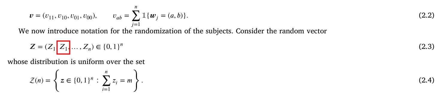
(S2) Randomization and observed data, p. 5: 'Consider the random vector $\boldsymbol{Z} = (Z_1, Z_1, \ldots, Z_n) \in \{0,1\}^n$ (2.3) whose distribution is uniform over the set $\mathcal{Z}(n) = \{\boldsymbol{z} \in \{0,1\}^n : \sum_{i=1}^{n} z_i = m\}$. (2.4) Here, the indices $i$ such that $Z_i = 1$ represent the subjects assigned to treatment. The vector of observed experimental outcomes $\boldsymbol{Y} = (Y_j)_{j=1}^{n}$ is then given by $Y_j = Z_j y_j(1) + (1 - Z_j) y_j(0)$. (2.5) We say that a table $\boldsymbol{w}$ is possible given the observed data $\boldsymbol{Y}$ if for every $j \in [\![1,n]\!]$, we have $\boldsymbol{w}_j(1) = Y_j$ if $Z_j = 1$, and $\boldsymbol{w}_j(0) = Y_j$ if $Z_j = 0$. We say that a count vector $\boldsymbol{v}$ is possible if it arises from some possible table $\boldsymbol{w}$.' [(2.3) prints $Z_1$ twice; the vector is $(Z_1, Z_2, \ldots, Z_n)$: finding P003-E015. The paper's results assume $1 \le m < n$.]
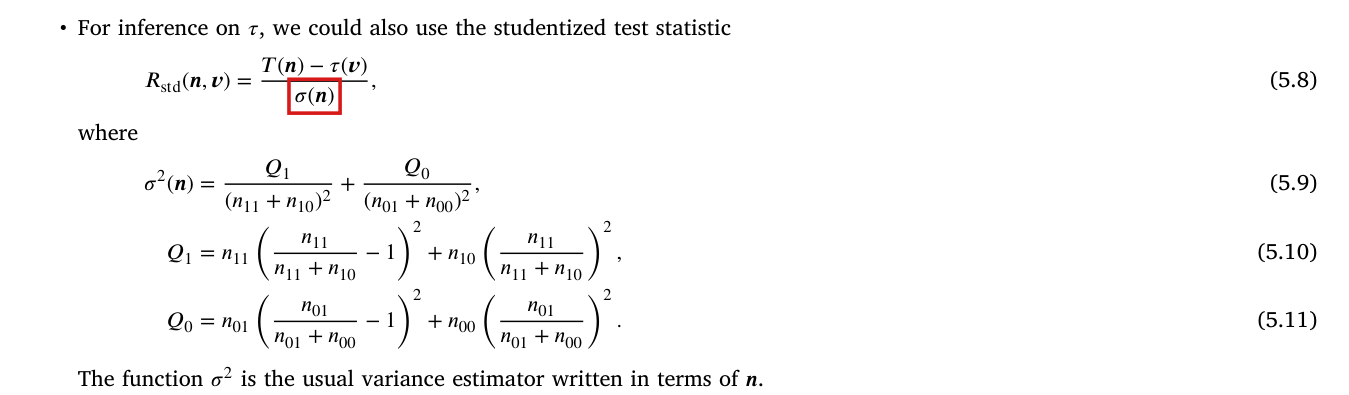
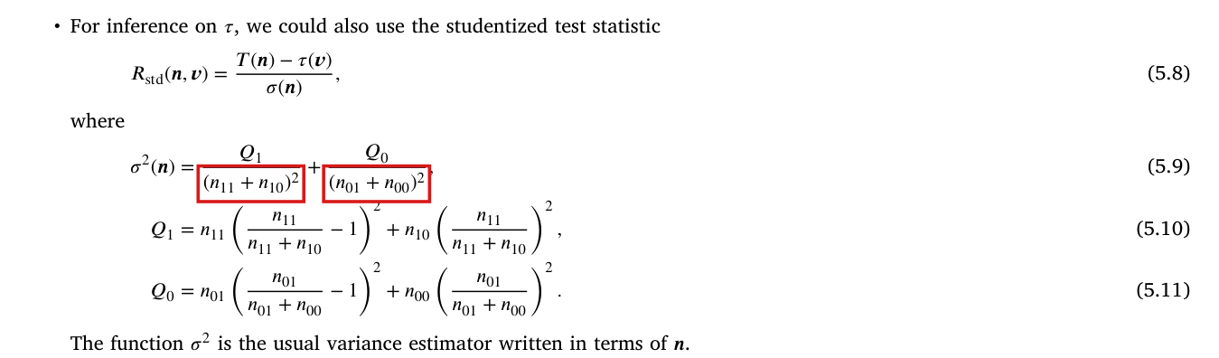
(S3) Estimand and estimator, p. 5: 'The sample average treatment effect for a potential outcome table is defined by $\tau(\boldsymbol{w}) = \frac{1}{n}\sum_{j=1}^{n}(w_j(1) - w_j(0))$. (2.6) The Neyman estimator of $\tau(\boldsymbol{y})$ is given by $T(\boldsymbol{Y},\boldsymbol{Z}) = \sum_{j=1}^{n}\frac{Z_j Y_j}{m} - \sum_{j=1}^{n}\frac{(1-Z_j)Y_j}{n-m}$. (2.7) This estimator depends on $(\boldsymbol{Y},\boldsymbol{Z})$ only through the observed count vector $\boldsymbol{n} \in \mathbb{Z}_{\ge 0}^{\{0,1\}^2}$ defined by $\boldsymbol{n} = (n_{11}, n_{10}, n_{01}, n_{00})$, $n_{zy} = \sum_{j=1}^{n}\mathbb{1}\{Z_j = z, Y_j = y\}$, (2.8) for $z \in \{0,1\}$ and $y \in \{0,1\}$. For example, $n_{10}$ is the number of subjects in the treatment group with observed outcome 0. Then $T(\boldsymbol{Y},\boldsymbol{Z}) = \frac{n_{11}}{m} - \frac{n_{01}}{n-m}$. We overload the notation slightly and write $T(\boldsymbol{n})$ for the value of the Neyman estimator $T(\boldsymbol{Y},\boldsymbol{Z})$, if $\boldsymbol{n}$ is the observed count vector for $(\boldsymbol{Y},\boldsymbol{Z})$.' 'We write $\log$ for the natural logarithm. When we use the base 2 logarithm, it is always denoted by $\log_2$. Additionally, we often abbreviate probability mass function as pmf.' In terms of the count vector, $\tau(\boldsymbol{v}) = (v_{10} - v_{01})/n$ ((4.2), p. 8: 'any possible count vector $\boldsymbol{v} = (v_{11},v_{10},v_{01},v_{00})$ such that $\tau(\boldsymbol{v}) = \tau_0$ satisfies the equations $v_{11}+v_{10}+v_{01}+v_{00} = n$, $v_{10} - v_{01} = n\tau_0$').
(S4) Candidate values, pp. 5-6: 'As $\boldsymbol{w}$ ranges over all tables, $\tau(\boldsymbol{w})$ takes every value in the set $\mathcal{S}(n) = \{-\frac{n}{n}, -\frac{n-1}{n}, \ldots, \frac{0}{n}, \ldots, \frac{n-1}{n}, \frac{n}{n}\}$, (2.9) which has $2n+1$ elements. After the experiment is completed, the set of $\tau(\boldsymbol{w})$ for $\boldsymbol{w}$ that are possible given the observed data is further restricted to $\mathcal{C}(\boldsymbol{Y},\boldsymbol{Z}) = \{\frac{1}{n}(\sum_{j=1}^{n}(2Z_j - 1)Y_j - m), \ldots, \frac{1}{n}(\sum_{j=1}^{n}(2Z_j-1)Y_j - m + n)\}$, (2.10) which has $n+1$ elements. We observe that $\mathcal{C}$ depends on $(\boldsymbol{Y},\boldsymbol{Z})$ only through the associated observed count vector $\boldsymbol{n}$.' [$\sum_j (2Z_j-1)Y_j = n_{11} - n_{01}$, so $n\,\mathcal{C}(\boldsymbol{n}) = [\![n_{11}-n_{01}-m,\; n_{11}-n_{01}-m+n]\!]$.]
(S5) Permutation p-value, Definition 2.1, p. 6: 'Let $\widetilde{\boldsymbol{Z}}$ be a random vector independent from $\boldsymbol{Z}$ with the same distribution, and let $\widetilde{\boldsymbol{Y}}$ be the vector with entries $\widetilde{Y}_j = \widetilde{Z}_j w_j(1) + (1 - \widetilde{Z}_j) w_j(0)$. (2.11) We say that $\boldsymbol{w}$ is compatible with observed data $(\boldsymbol{Y},\boldsymbol{Z})$ at level $1-\alpha$ if $p(\boldsymbol{w},\boldsymbol{Y},\boldsymbol{Z}) = \mathbb{P}(|T(\widetilde{\boldsymbol{Y}},\widetilde{\boldsymbol{Z}}) - \tau(\boldsymbol{w})| \ge |T(\boldsymbol{Y},\boldsymbol{Z}) - \tau(\boldsymbol{w})|) \ge \alpha$. (2.12) We say that $\boldsymbol{w}$ is compatible with an observed count vector $\boldsymbol{n}$ if (2.12) holds with $T(\boldsymbol{Y},\boldsymbol{Z})$ replaced by $T(\boldsymbol{n})$.' 'Let $\boldsymbol{v}$ denote the count vector associated with $\boldsymbol{w}$, as defined in (2.2), and let $\boldsymbol{n}$ be as in (2.8). Then it is straightforward to see that $p(\boldsymbol{w},\boldsymbol{Y},\boldsymbol{Z})$ depends on $(\boldsymbol{w},\boldsymbol{Y},\boldsymbol{Z})$ only through the count vectors $\boldsymbol{n}$ and $\boldsymbol{v}$. This motivates the shorthand $p(\boldsymbol{v},\boldsymbol{n}) = p(\boldsymbol{w},\boldsymbol{Y},\boldsymbol{Z})$.' [The probability in (2.12) is over $\widetilde{\boldsymbol{Z}}$ alone, with $(\boldsymbol{Y},\boldsymbol{Z})$ held fixed.] Algorithm 2.2, p. 6: 'A permutation test takes as inputs $\alpha \in (0,1)$, a count vector $\boldsymbol{v}$, and a vector $\boldsymbol{n} \in \mathbb{Z}_{\ge 0}^{\{0,1\}^2}$. It returns a binary decision, accept or reject, as follows. The algorithm computes $p(\boldsymbol{v},\boldsymbol{n})$ by direct enumeration of all $\binom{n}{m}$ elements of the set $\mathcal{Z}(n)$ (defined in Eq. (2.4)), over which $\widetilde{\boldsymbol{Z}}$ is uniformly distributed. If $p(\boldsymbol{v},\boldsymbol{n}) \ge \alpha$, it accepts. Otherwise, it rejects.'
(S6) The interval $\mathcal{I}_\alpha$, p. 6: 'Given an observed count vector $\boldsymbol{n}$, set $\mathcal{T}(\boldsymbol{n}) = \{(i,j,k,l) : i \in [\![0,n_{11}]\!], j \in [\![0,n_{10}]\!], k \in [\![0,n_{01}]\!], l \in [\![0,n_{00}]\!]\}$. (2.13) We define vectors $\boldsymbol{v}(i,j,k,l)$ in the following way. Given $(i,j,k,l) \in \mathcal{T}(\boldsymbol{n})$, set $\boldsymbol{v}(i,j,k,l) = (i+k,\; n_{11}-i+l,\; n_{01}-k+j,\; n_{10}+n_{00}-j-l)$. (2.14)' '[...] the collection of $\boldsymbol{v}(i,j,k,l)$ such that $(i,j,k,l) \in \mathcal{T}(\boldsymbol{n})$ is exactly the set of count vectors $\boldsymbol{v}$ possible given the observed count vector $\boldsymbol{n}$.' 'Algorithm 2.3. This algorithm takes as input $\alpha \in (0,1)$ and a vector $\boldsymbol{n} \in \mathbb{Z}_{\ge 0}^{\{0,1\}^2}$. It returns an interval $\mathcal{I}_\alpha(\boldsymbol{n}) = [L_\alpha(\boldsymbol{n}), U_\alpha(\boldsymbol{n})]$. By directly enumerating of all elements of $\mathcal{T}$, and applying Algorithm 2.2 to each one, compute the set $\mathcal{K}(\boldsymbol{n}) = \{\tau(\boldsymbol{v}(i,j,k,l)) : (i,j,k,l) \in \mathcal{T}(\boldsymbol{n}) \text{ and Algorithm 2.2 accepts } \boldsymbol{v}(i,j,k,l)\}$. (2.15) Return $U_\alpha(\boldsymbol{n}) = \max(\mathcal{K})$ and $L_\alpha = \min(\mathcal{K})$.' 'Then using Algorithm 2.3, we define $\mathcal{I}_\alpha(\boldsymbol{Y},\boldsymbol{Z}) = [L_\alpha(\boldsymbol{Y},\boldsymbol{Z}), U_\alpha(\boldsymbol{Y},\boldsymbol{Z})]$ (2.16) by setting $\mathcal{I}_\alpha(\boldsymbol{Y},\boldsymbol{Z}) = \mathcal{I}_\alpha(\boldsymbol{n})$.' [The paper does not say what is returned if $\mathcal{K}(\boldsymbol{n})$ is empty, and it shows that $\mathcal{K}(\boldsymbol{n})$ is non-empty only for balanced designs, where it contains $T(\boldsymbol{n})$ by Lemma 3.1. A formal statement about an unbalanced design must either prove non-emptiness or fix a convention; for coverage statements, data with empty $\mathcal{K}(\boldsymbol{n})$ count as not covering.]
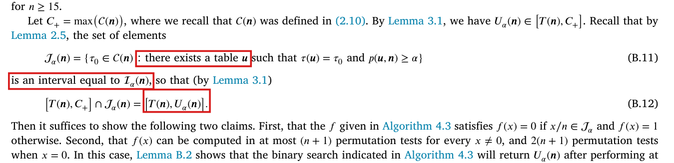
(S7) Cited lemmas, p. 7: 'Lemma 2.4 (Li and Ding, 2016, Theorem 1). A potential outcome table $\boldsymbol{w}$ with count vector $\boldsymbol{v}$ is possible given an observed count vector $\boldsymbol{n}$ if and only if $\max(0,\; n_{11}-v_{10},\; v_{11}-n_{01},\; v_{11}+v_{01}-n_{10}-n_{01}) \le \min(v_{11},\; n_{11},\; v_{11}+v_{01}-n_{01},\; n-v_{10}-n_{01}-n_{10})$. (2.17)' 'Lemma 2.5 (Li and Ding, 2016, Theorem A.4). Suppose $n = 2m$. Fix $\alpha \in (0,1)$ and observed data $\boldsymbol{Y}$ and $\boldsymbol{Z}$. For every $\tau_0 \in \mathcal{I}_\alpha(\boldsymbol{Y},\boldsymbol{Z}) \cap \mathcal{C}$, there exists a possible potential outcome table $\boldsymbol{w}$ such that $\tau(\boldsymbol{w}) = \tau_0$ and $p(\boldsymbol{w},\boldsymbol{Y},\boldsymbol{Z}) \ge \alpha$.'
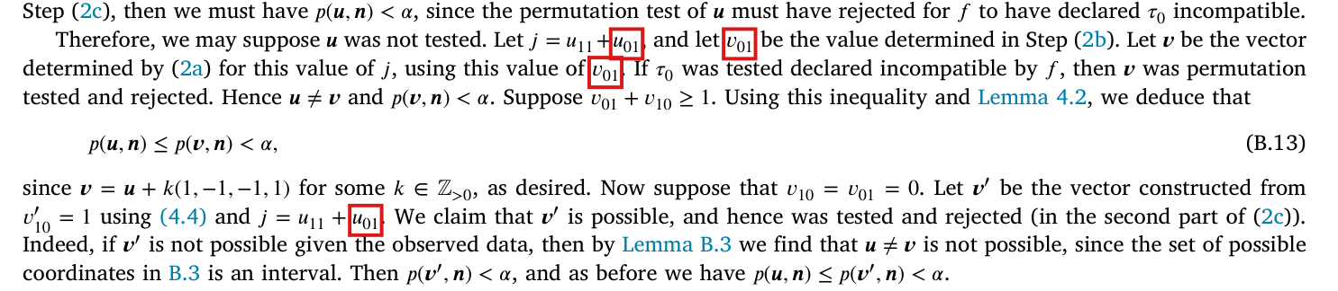
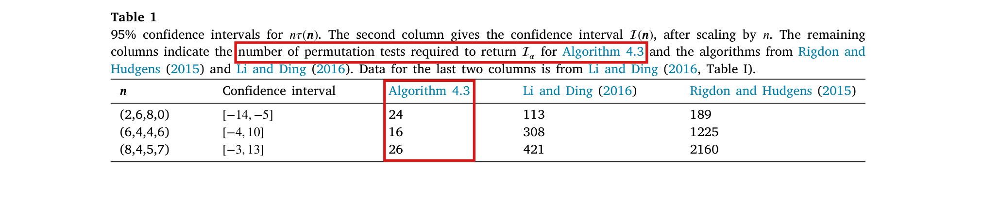
(S8) Balanced exact algorithm, p. 8: 'Algorithm 4.3. This algorithm takes as input $\alpha \in (0,1)$ and a vector $\boldsymbol{n} \in \mathbb{Z}_{\ge 0}^{\{0,1\}^2}$. It returns an interval $[L^{(1)}_\alpha(\boldsymbol{n}), U^{(1)}_\alpha(\boldsymbol{n})]$. We give only the steps for finding $U^{(1)}_\alpha(\boldsymbol{n})$, since finding $L^{(1)}_\alpha(\boldsymbol{n})$ is analogous. We perform a binary search using a function $f : [\![nT(\boldsymbol{n}),\, n\max(\mathcal{C}(\boldsymbol{n}))]\!] \to \{0,1\}$ defined below. The precise definition of this binary search is given as Algorithm B.1 in Appendix B.1. Given an input $x$, the function $f$ returns 0 if $x/n$ is compatible with the vector $\boldsymbol{n}$, and 1 otherwise, where the compatibility of a given $\tau_0 \in \mathcal{C}(\boldsymbol{n})$ is determined through the following steps. 1. Initialize $j \leftarrow 0$. 2. If $j \le n$, perform the following steps. (a) Construct a count vector $\boldsymbol{v}$ as follows (recall Eq. (2.2)). Let $v_{10}$ be a free parameter, and set $v_{11} = j - v_{10}$. Then (solving Eq. (4.2)) we set $v_{01} = v_{10} - n\tau_0$, $v_{00} = n - j - v_{10} + n\tau_0$. (4.4) (b) Find the smallest $v_{10}$ that leads to a possible table $\boldsymbol{v}$ given the observed data $\boldsymbol{n}$. This can be done in constant time using Lemma B.3, stated in Appendix B.1 below. If no value of $v_{10}$ leads to a possible table, set $j \leftarrow j+1$ and go to (2). (c) Permutation test the count vector $\boldsymbol{v}$ coming from the choice of $v_{10}$ in the previous step using Algorithm 2.2 with the given value of $\alpha$. If $\boldsymbol{v}$ is accepted, return that $\tau_0$ is compatible. If $\boldsymbol{v}$ is rejected and $v_{10} \ge 1$ or $v_{01} \ge 1$, set $j \leftarrow j+1$ and go to (2). If $\boldsymbol{v}$ is rejected and $v_{10} = v_{01} = 0$, additionally permutation test the count vector given by $v_{10} = 1$. If it is possible and accepted, terminate the algorithm and declare $\tau_0$ compatible. Otherwise, set $j \leftarrow j+1$ and go to (2). 3. Return that $\tau_0$ is incompatible.'
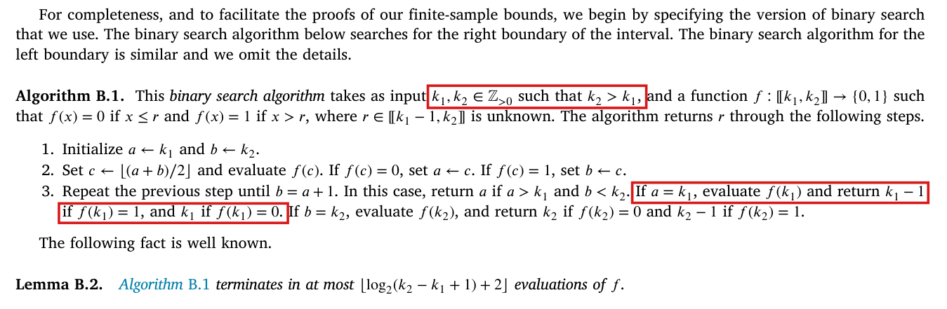
(S9) Binary search and possibility along a line, Appendix B.1, p. 20: 'Algorithm B.1. This binary search algorithm takes as input $k_1, k_2 \in \mathbb{Z}_{>0}$ such that $k_2 > k_1$, and a function $f : [\![k_1,k_2]\!] \to \{0,1\}$ such that $f(x) = 0$ if $x \le r$ and $f(x) = 1$ if $x > r$, where $r \in [\![k_1 - 1, k_2]\!]$ is unknown. The algorithm returns $r$ through the following steps. 1. Initialize $a \leftarrow k_1$ and $b \leftarrow k_2$. 2. Set $c \leftarrow \lfloor (a+b)/2 \rfloor$ and evaluate $f(c)$. If $f(c) = 0$, set $a \leftarrow c$. If $f(c) = 1$, set $b \leftarrow c$. 3. Repeat the previous step until $b = a+1$. In this case, return $a$ if $a > k_1$ and $b < k_2$. If $a = k_1$, evaluate $f(k_1)$ and return $k_1 - 1$ if $f(k_1) = 1$, and $k_1$ if $f(k_1) = 0$. If $b = k_2$, evaluate $f(k_2)$, and return $k_2$ if $f(k_2) = 0$ and $k_2 - 1$ if $f(k_2) = 1$.' 'Lemma B.2. Algorithm B.1 terminates in at most $\lfloor \log_2(k_2 - k_1 + 1) + 2 \rfloor$ evaluations of $f$.' 'Lemma B.3. Fix $j, v_{10} \in \mathbb{Z}_{\ge 0}$ and $\tau_0 \in \mathcal{C}$, and consider the potential outcome vector $\boldsymbol{v} = (j - v_{10},\; v_{10},\; v_{10} - n\tau_0,\; n - j - v_{10} + n\tau_0)$. (B.1) Given observed data $\boldsymbol{n}$, a necessary condition for $\boldsymbol{v}$ to be possible is that all of the following inequalities hold: $j \ge n\tau_0 + n_{01}$, $j \ge n_{11}$, $n \ge j + n_{10}$, $n_{11} + n\tau_0 + n_{10} + n_{01} \ge j$. (B.2) In this case, the possible values of $v_{10}$ are given by the interval $\max(0,\; n\tau_0,\; j - n_{11} - n_{01},\; n_{11} + n_{01} + n\tau_0 - j) \le v_{10} \le \min(j,\; n_{11} + n_{00},\; n_{10} + n_{01} + n\tau_0,\; n + n\tau_0 - j)$, (B.3) which may be empty.'
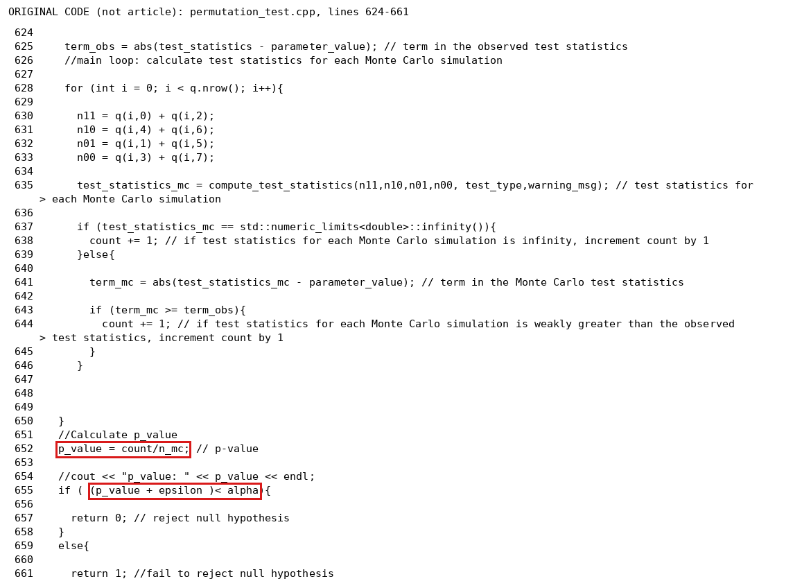
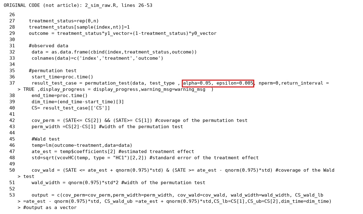
(S10) Balanced Monte Carlo algorithm, Section 4.2, p. 9: 'Given a count vector $\boldsymbol{v}$, we define $\widetilde{\boldsymbol{w}} = \widetilde{\boldsymbol{w}}(\boldsymbol{v})$ as the potential outcome table such that $\widetilde{\boldsymbol{w}}_j = (1,1)$, $j = 1,\ldots,v_{11}$; $\widetilde{\boldsymbol{w}}_j = (1,0)$, $j = v_{11}+1,\ldots,v_{11}+v_{10}$; $\widetilde{\boldsymbol{w}}_j = (0,1)$, $j = v_{11}+v_{10}+1,\ldots,v_{11}+v_{10}+v_{01}$; $\widetilde{\boldsymbol{w}}_j = (0,0)$, $j = v_{11}+v_{10}+v_{01}+1,\ldots,n$. (4.5)' 'Algorithm 4.4. Take as input $\alpha \in (0,1)$, $\varepsilon \in [0,\alpha)$, $K \in \mathbb{Z}_{>0}$, a count vector $\boldsymbol{v} \in \mathbb{Z}_{\ge 0}^{\{0,1\}^2}$, and a vector $\boldsymbol{n} \in \mathbb{Z}_{\ge 0}^{\{0,1\}^2}$. The algorithm will return a binary decision, either accept or reject. Let $\boldsymbol{Z}^{(1)},\ldots,\boldsymbol{Z}^{(K)}$ be a sequence of independent, identically distributed random vectors, with common distribution equal to that of $\boldsymbol{Z}$. Define random variables $V_1,\ldots,V_K$ by $V_i = \mathbb{1}(|T(\boldsymbol{n}^{(i)}) - \tau(\widetilde{\boldsymbol{w}})| \ge |T(\boldsymbol{n}) - \tau(\widetilde{\boldsymbol{w}})|)$, $i \in [\![1,K]\!]$, (4.6) where $\boldsymbol{n}^{(i)}$ is the outcome count vector corresponding to $(\boldsymbol{Y}^{(i)},\boldsymbol{Z}^{(i)})$, with $\boldsymbol{Y}^{(i)}$ defined by $Y^{(i)}_j = Z^{(i)}_j \widetilde{w}_j(1) + (1 - Z^{(i)}_j)\widetilde{w}_j(0)$ (4.7) for all $j \in [\![1,n]\!]$. Set $S = \frac{1}{K}\sum_{i=1}^{K} V_i$. (4.8) Simulate a realization of $S$ by simulating realizations of the $K$ variables $\boldsymbol{Z}^{(1)},\ldots,\boldsymbol{Z}^{(K)}$, and constructing the $V_i$ and $S$ accordingly. Return the decision accept if $S + \varepsilon \ge \alpha$, and return the decision reject otherwise.' 'Algorithm 4.5. This algorithm takes as input $\alpha \in (0,1)$, $\varepsilon \in [0,\alpha)$, and a vector $\boldsymbol{n} \in \mathbb{Z}_{\ge 0}^{\{0,1\}^2}$. It returns an interval $\mathcal{I}_{\alpha,\varepsilon,K}(\boldsymbol{n}) = [L_{\alpha,\varepsilon,K}(\boldsymbol{n}), U_{\alpha,\varepsilon,K}(\boldsymbol{n})]$. The algorithm is identical to Section 4, except every use of an exact permutation test (Algorithm 2.2) is replaced with an approximate permutation test with the given parameters (Algorithm 4.4). A new set of independent vectors $\boldsymbol{Z}^{(1)},\ldots,\boldsymbol{Z}^{(k)}$ is generated for each approximate permutation test (independently of the permutation vectors used for any previous tests).' 'Given observed data $(\boldsymbol{Y},\boldsymbol{Z})$ we define the interval $\mathcal{I}_{\alpha,\varepsilon,K}(\boldsymbol{Y},\boldsymbol{Z})$ to be the interval $\mathcal{I}_{\alpha,\varepsilon,K}(\boldsymbol{n})$ returned by Algorithm 4.5 for the observed count vector $\boldsymbol{n}$ corresponding to $(\boldsymbol{Y},\boldsymbol{Z})$.' ['identical to Section 4' means identical to Algorithm 4.3, and $K \in \mathbb{Z}_{>0}$ is also an input: finding P003-N005, cross-references.]
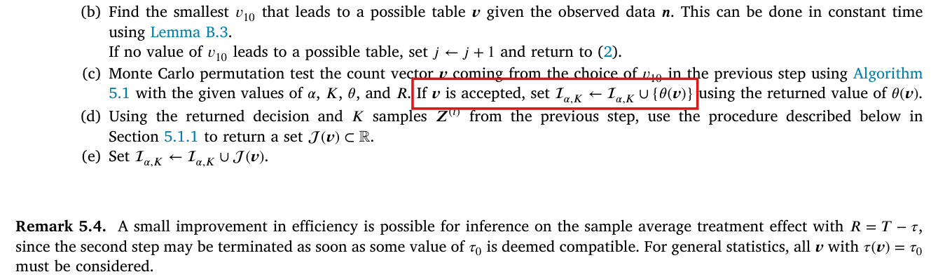
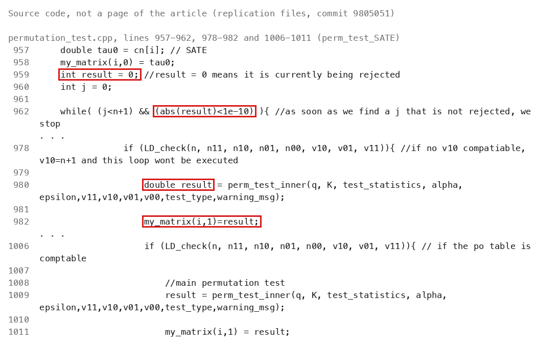
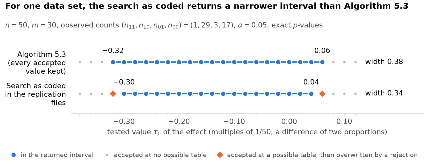
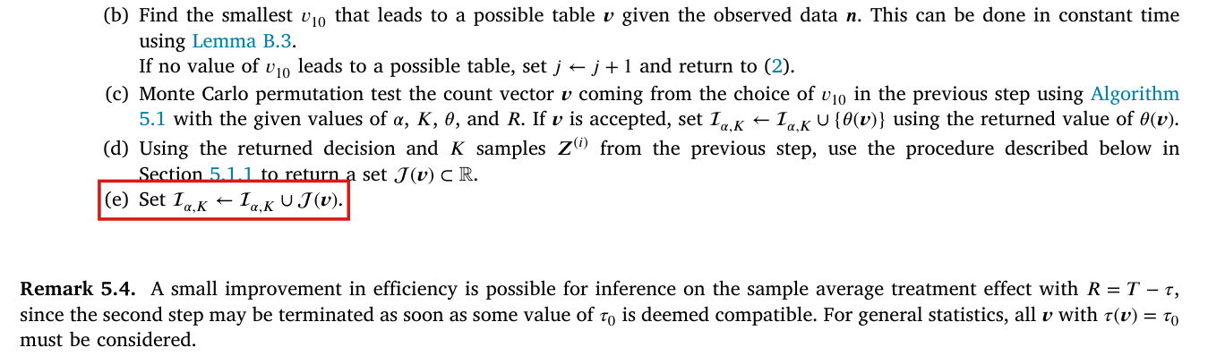
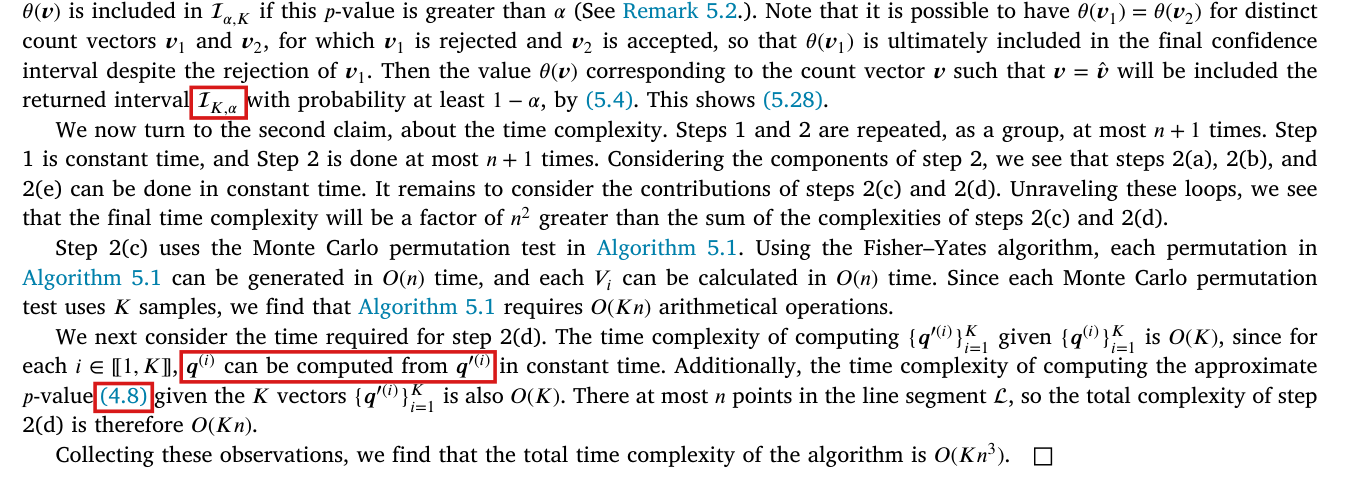
(S11) General Monte Carlo algorithm, Section 5.1, pp. 10-13: estimand $\theta : \mathbb{Z}_{\ge 0}^{\{0,1\}^2} \to \mathbb{R}$ and test statistic $R : \mathbb{Z}_{\ge 0}^{\{0,1\}^2} \times \mathbb{Z}_{\ge 0}^{\{0,1\}^2} \to \mathbb{R}$ ('Estimands $\theta$ will take potential outcome count vectors $\boldsymbol{v}$ as arguments, and test statistics $R$ will take pairs $(\boldsymbol{n},\boldsymbol{v})$ of observed count vectors $\boldsymbol{n}$ and count vectors $\boldsymbol{v}$ as arguments'). 'Algorithm 5.1. Take as input $\alpha \in (0,1)$, $K \in \mathbb{Z}_{>0}$, an estimand $\theta$, a test statistic $R$, a count vector $\boldsymbol{v} \in \mathbb{Z}_{\ge 0}^{\{0,1\}^2}$, and a vector $\boldsymbol{n} \in \mathbb{Z}_{\ge 0}^{\{0,1\}^2}$. The algorithm will return a binary decision, either accept or reject, the value $\theta(\boldsymbol{v})$, and $K$ vectors lying in $\mathcal{Z}(n)$. Let $\boldsymbol{Z}^{(1)},\ldots,\boldsymbol{Z}^{(K)}$ be a sequence of independent, identically distributed random vectors, with common distribution equal to that of $\boldsymbol{Z}$. Define random variables $V_1,\ldots,V_K$ by $V_i = \mathbb{1}(|R(\boldsymbol{n}^{(i)},\boldsymbol{v})| \ge |R(\boldsymbol{n},\boldsymbol{v})|)$, $i \in [\![1,K]\!]$, (5.1) where $\boldsymbol{n}^{(i)}$ is the outcome count vector corresponding to $(\boldsymbol{Y}^{(i)},\boldsymbol{Z}^{(i)})$, with $\boldsymbol{Y}^{(i)}$ defined by $Y^{(i)}_j = Z^{(i)}_j\widetilde{w}_j(1) + (1 - Z^{(i)}_j)\widetilde{w}_j(0)$ (5.2) for all $j \in [\![1,n]\!]$, and we recall the definition of $\widetilde{\boldsymbol{w}}$ from Eq. (4.5). Set $S = \frac{1}{K+1}(1 + \sum_{i=1}^{K} V_i)$. (5.3) [...] Return the decision accept if $S > \alpha$, and return the decision reject otherwise. Also return $\theta(\boldsymbol{v})$ and the realized values of $\boldsymbol{Z}^{(1)},\ldots,\boldsymbol{Z}^{(K)}$.' 'Algorithm 5.3. This algorithm takes as input $\alpha \in (0,1)$, $K \in \mathbb{Z}_{>0}$, a vector $\boldsymbol{n} \in \mathbb{Z}_{\ge 0}^{\{0,1\}^2}$, an estimand $\theta$, and a test statistic $R$. It returns a confidence set $\mathcal{I}_{\alpha,K}$. We initialize $\mathcal{I}_{\alpha,K} \leftarrow \varnothing$. For every $\tau_0 \in \mathcal{C}(\boldsymbol{n})$, in descending order from $\max(\mathcal{C}(\boldsymbol{n}))$, we perform the following steps. 1. Initialize $j \leftarrow 0$. 2. If $j \le n$, perform the following steps. (a) Construct a count vector $\boldsymbol{v}$ as follows (recall Eq. (2.2)). Let $v_{10}$ be a free parameter, and set $v_{11} = j - v_{10}$. Then (solving Eq. (4.2)) we set $v_{01} = v_{10} - n\tau_0$, $v_{00} = n - j - v_{10} + n\tau_0$. (5.16) (b) Find the smallest $v_{10}$ that leads to a possible table $\boldsymbol{v}$ given the observed data $\boldsymbol{n}$. This can be done in constant time using Lemma B.3. If no value of $v_{10}$ leads to a possible table, set $j \leftarrow j+1$ and return to (2). (c) Monte Carlo permutation test the count vector $\boldsymbol{v}$ coming from the choice of $v_{10}$ in the previous step using Algorithm 5.1 with the given values of $\alpha$, $K$, $\theta$, and $R$. If $\boldsymbol{v}$ is accepted, set $\mathcal{I}_{\alpha,K} \leftarrow \mathcal{I}_{\alpha,K} \cup \{\theta(\boldsymbol{v})\}$ using the returned value of $\theta(\boldsymbol{v})$. (d) Using the returned decision and $K$ samples $\boldsymbol{Z}^{(i)}$ from the previous step, use the procedure described below in Section 5.1.1 to return a set $\mathcal{J}(\boldsymbol{v}) \subset \mathbb{R}$. (e) Set $\mathcal{I}_{\alpha,K} \leftarrow \mathcal{I}_{\alpha,K} \cup \mathcal{J}(\boldsymbol{v})$.' Section 5.1.1, p. 12: 'For all $k \in \mathbb{Z}_{>0}$, denote $\boldsymbol{v}_k = (v_{11}-k,\; v_{10}+k,\; v_{01}+k,\; v_{00}-k)$ (5.17) and let $\mathcal{L} = \{\boldsymbol{v}_k : k \in [\![1,n]\!], \boldsymbol{v}_k \text{ is possible given } \boldsymbol{n}\}$. (5.18)'; the draws for $\boldsymbol{v}$ are converted by the random update (5.19)-(5.26) into draws for $\boldsymbol{v}' = \boldsymbol{v} + (-1,1,1,-1)$ (printed '$(-1,1,1-1)$'), iterated along $\mathcal{L}$; $\mathcal{V}$ is the set of $\boldsymbol{v}_k \in \mathcal{L}$ that 'are both possible and would be accepted by an application of Algorithm 5.1', and $\mathcal{J} = \{\theta(\boldsymbol{v}) : \boldsymbol{v} \in \mathcal{V}\}$ (5.27). 'As in (2.16), we use $\mathcal{I}_{\alpha,K}(\boldsymbol{Y},\boldsymbol{Z})$ as shorthand for $\mathcal{I}_{\alpha,K}(\boldsymbol{n})$, where $\boldsymbol{n}$ is the count vector for $(\boldsymbol{Y},\boldsymbol{Z})$.'
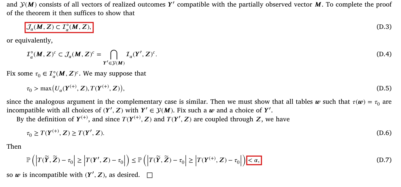
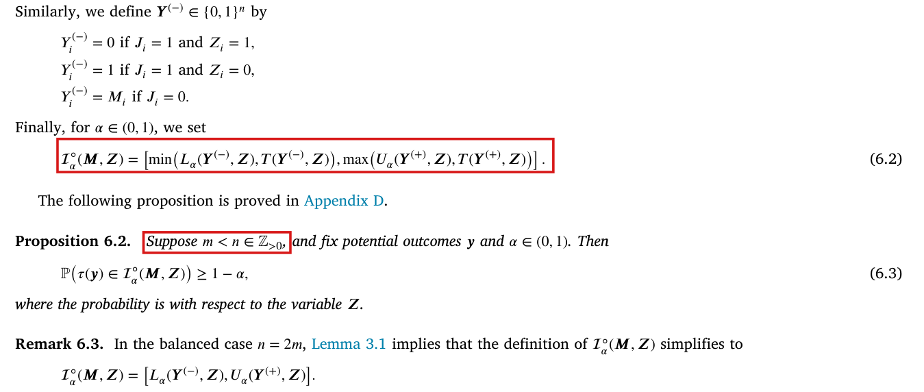
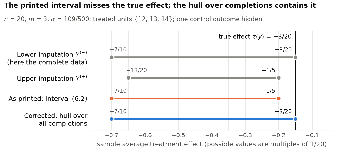
(S12) Missing data, Section 6, pp. 13-14: 'we suppose that instead of observing $(\boldsymbol{Y},\boldsymbol{Z})$, the experimenter observes $(\boldsymbol{M},\boldsymbol{Z})$, where $\boldsymbol{M} \in \{-1,0,1\}^n$, $M_i = -J_i + (1 - J_i)Y_i$, (6.1) and $\boldsymbol{J} \in \{1,0\}^n$. Here $\boldsymbol{J}$ is a random variable which may have an arbitrary distribution, and in particular may depend on $\boldsymbol{Y}$ and $\boldsymbol{Z}$. The indices $i$ such that $J_i = 0$ denote realized outcomes that are observed, while those such that $J_i = 1$ indicate missing data. Hence, we have $M_i = -1$ if the realized outcome for the $i$th subject is not observed.' 'Definition 6.1. Given a observed data $(\boldsymbol{M},\boldsymbol{Z})$, we define the vector $\boldsymbol{Y}^{(+)} \in \{0,1\}^n$ by $Y^{(+)}_i = 1$ if $J_i = 1$ and $Z_i = 1$, $Y^{(+)}_i = 0$ if $J_i = 1$ and $Z_i = 0$, $Y^{(+)}_i = M_i$ if $J_i = 0$. Similarly, we define $\boldsymbol{Y}^{(-)} \in \{0,1\}^n$ by $Y^{(-)}_i = 0$ if $J_i = 1$ and $Z_i = 1$, $Y^{(-)}_i = 1$ if $J_i = 1$ and $Z_i = 0$, $Y^{(-)}_i = M_i$ if $J_i = 0$. Finally, for $\alpha \in (0,1)$, we set $\mathcal{I}^{\circ}_\alpha(\boldsymbol{M},\boldsymbol{Z}) = [\min(L_\alpha(\boldsymbol{Y}^{(-)},\boldsymbol{Z}), T(\boldsymbol{Y}^{(-)},\boldsymbol{Z})),\; \max(U_\alpha(\boldsymbol{Y}^{(+)},\boldsymbol{Z}), T(\boldsymbol{Y}^{(+)},\boldsymbol{Z}))]$. (6.2)'
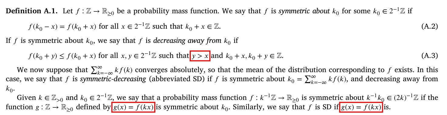
(S13) Symmetric-decreasing pmfs, Appendix A, p. 18: 'For $k \in \mathbb{Z}_{>0}$, we denote $k^{-1}\mathbb{Z} = \{\frac{j}{k} : j \in \mathbb{Z}\}$, $k^{-1}(2\mathbb{Z}) = \{\frac{2j}{k} : j \in \mathbb{Z}\}$, $k^{-1}(2\mathbb{Z}+1) = \{\frac{2j+1}{k} : j \in \mathbb{Z}\}$. (A.1) Definition A.1. Let $f : \mathbb{Z} \to \mathbb{R}_{\ge 0}$ be a probability mass function. We say that $f$ is symmetric about $k_0$ for some $k_0 \in 2^{-1}\mathbb{Z}$ if $f(k_0 - x) = f(k_0 + x)$ for all $x \in 2^{-1}\mathbb{Z}$ such that $k_0 + x \in \mathbb{Z}$. (A.2) If $f$ is symmetric about $k_0$, we say that $f$ is decreasing away from $k_0$ if $f(k_0 + y) \le f(k_0 + x)$ for all $x, y \in 2^{-1}\mathbb{Z}$ such that $y > x$ and $k_0 + x, k_0 + y \in \mathbb{Z}$. (A.3) We now suppose that $\sum_{k=-\infty}^{\infty} k f(k)$ converges absolutely, so that the mean of the distribution corresponding to $f$ exists. In this case, we say that $f$ is symmetric-decreasing (abbreviated SD) if $f$ is symmetric about $k_0 = \sum_{k=-\infty}^{\infty} k f(k)$, and decreasing away from $k_0$. Given $k \in \mathbb{Z}_{>0}$ and $k_0 \in 2^{-1}\mathbb{Z}$, we say that a probability mass function $f : k^{-1}\mathbb{Z} \to \mathbb{R}_{\ge 0}$ is symmetric about $k^{-1}k_0 \in (2k)^{-1}\mathbb{Z}$ if the function $g : \mathbb{Z} \to \mathbb{R}_{\ge 0}$ defined by $g(x) = f(kx)$ is symmetric about $k_0$. Similarly, we say that $f$ is SD if $g(x) = f(kx)$ is.' 'Recall from (2.1) that $\boldsymbol{w}$ denotes a generic potential outcome table. We use the notation $T(\boldsymbol{w},\boldsymbol{Z})$ to stand for $T(\boldsymbol{Y},\boldsymbol{Z})$ with $Y$ generated using the potential outcomes $\boldsymbol{w}$ and the treatment assignments given by $\boldsymbol{Z}$. Since this quantity depends on $\boldsymbol{w}$ only through its associated count vector $\boldsymbol{v}$, we also write $T(\boldsymbol{v},\boldsymbol{Z})$ for $T(\boldsymbol{n},\boldsymbol{Z})$.' [As printed, (A.3) lacks the restriction $0 \le x$, and the rescaling should be $g(x) = f(x/k)$: finding P003-E006, target P003-T14. Throughout the targets, 'SD' means the corrected definition: symmetric about the mean and non-increasing in the distance from the mean, on the stated lattice. '$T(\boldsymbol{n},\boldsymbol{Z})$' should read '$T(\boldsymbol{w},\boldsymbol{Z})$' (finding P003-N017), and it is the distribution of $T(\boldsymbol{w},\boldsymbol{Z})$, not its value at a fixed labeled assignment, that depends on $\boldsymbol{w}$ only through $\boldsymbol{v}$ (finding P003-E015).]
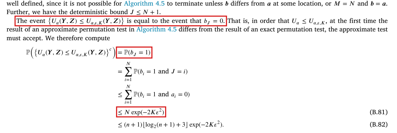
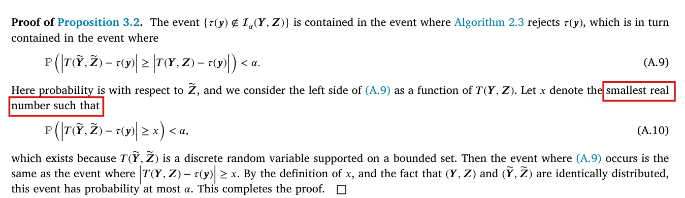
Effective claim (source TeX): Printed statements refuted (proof of Lemma B.15). 'We begin by bounding the probability that $U_\alpha(\boldsymbol{Y},\boldsymbol{Z}) \le U_{\alpha,\varepsilon,K}(\boldsymbol{Y},\boldsymbol{Z})$ does not hold. Let $N$ be the total number of permutation tests performed by Algorithm 4.3 in the course of finding $U_\alpha(\boldsymbol{Y},\boldsymbol{Z})$. Letting 0 represent acceptance and 1 represent rejection, we let $\boldsymbol{a} = (a_i)_{i=1}^{N} \in \{0,1\}^N$ denote the sequences of acceptances and rejections made by the permutation tests in Algorithm 4.3. We condition on the observed data $(\boldsymbol{Y},\boldsymbol{Z})$, so that $\boldsymbol{a}$ becomes deterministic. Given this observed data, let $M$ denote the (random) number of approximate permutations performed by Algorithm 4.5 before returning $U_{\alpha,\varepsilon,K}(\boldsymbol{Y},\boldsymbol{Z})$. Let $\boldsymbol{b} = (b_i)_{i=1}^{M} \in \{0,1\}^M$ denote the corresponding (random) sequence of acceptances and rejections. Let $J$ be a random variable denoting the smallest positive integer such that $a_J \ne b_J$. If $a_i = b_i$ for all $i \in [\![1,N]\!]$, in which case $U_\alpha = U_{\alpha,\varepsilon,K}$, we set $J = N+1$ and define $b_J = 0$. [...] The event $\{U_\alpha(\boldsymbol{Y},\boldsymbol{Z}) \le U_{\alpha,\varepsilon,K}(\boldsymbol{Y},\boldsymbol{Z})\}$ is equal to the event that $b_J = 0$. That is, in order that $U_\alpha \le U_{\alpha,\varepsilon,K}$, at the first time the result of an approximate permutation test in Algorithm 4.5 differs from the result of an exact permutation test, the approximate test must accept. We therefore compute $\mathbb{P}(\{U_\alpha(\boldsymbol{Y},\boldsymbol{Z}) \le U_{\alpha,\varepsilon,K}(\boldsymbol{Y},\boldsymbol{Z})\}^c) = \mathbb{P}(b_J = 1) = \sum_{i=1}^{N}\mathbb{P}(b_i = 1 \text{ and } J = i) \le \sum_{i=1}^{N}\mathbb{P}(b_i = 1 \text{ and } a_i = 0) \le N\exp(-2K\varepsilon^2)$ (B.81) $\le (n+1)\lfloor \log_2(n+1) + 3 \rfloor \exp(-2K\varepsilon^2)$. (B.82)' (p. 27.) 'For the proof of the second claim, we keep the notation $\boldsymbol{a}$ and $\boldsymbol{b}$, but now define $\boldsymbol{a}$ using the interval $\mathcal{I}_{\alpha-2\varepsilon}(\boldsymbol{Y},\boldsymbol{Z})$. [...] The event $\{U_{\alpha-2\varepsilon}(\boldsymbol{Y},\boldsymbol{Z}) \ge U_{\alpha,\varepsilon,K}(\boldsymbol{Y},\boldsymbol{Z})\}$ is equal to the event $\{b_J = 1\} \cup \{J = N+1\}$. (B.85) We compute $\mathbb{P}(\{U_{\alpha-2\varepsilon}(\boldsymbol{Y},\boldsymbol{Z}) \ge U_{\alpha,\varepsilon,K}(\boldsymbol{Y},\boldsymbol{Z})\}^c) = \mathbb{P}(b_J = 0 \text{ and } J \le N)$ (B.86) $= \sum_{i=1}^{N}\mathbb{P}(b_i = 0 \text{ and } J = i)$ (B.87) $\le \sum_{i=1}^{N}\mathbb{P}(b_i = 0 \text{ and } a_i = 1)$ (B.88) $\le N\exp(-2K\varepsilon^2)$ (B.89) $\le (n+1)\lfloor \log_2(n+1) + 3 \rfloor \exp(-2K\varepsilon^2)$. (B.90)' (p. 28.)
Counterexample (validator v1; exact rational arithmetic). $n = 30$, $m = 15$, $\boldsymbol{n} = (n_{11},n_{10},n_{01},n_{00}) = (2,13,1,14)$, $\alpha = 1/20$, $\varepsilon = 1/200$, $K = 1$. (These data have positive probability, for example $45/116$ under a true table with count vector $(3,0,0,27)$.) Then $T(\boldsymbol{n}) = 1/15$, $n\,\mathcal{C}(\boldsymbol{n}) = [\![-14,16]\!]$, and the upper search runs on $[\![2,16]\!]$ (positive endpoints, as Algorithm B.1 requires). With $K = 1$, $S \in \{0,1\}$ and Algorithm 4.4 accepts exactly when $S = 1$.
Exact search (Algorithm 4.3 with Algorithm B.1; p-values $p(\boldsymbol{v},\boldsymbol{n})$): at $x = 9$ it rejects $(1,9,0,20)$ ($p = 412/10005 < 1/20$) and accepts $(2,9,0,19)$ ($p = 752/10005 \ge 1/20$); at $x = 12$ it rejects all five tested vectors $(1,12,0,17)$, $(2,12,0,16)$, $(3,12,0,15)$, $(3,13,1,13)$, $(3,14,2,11)$ (p-values $407/190095$, $18854/3231615$, $3847/340170$, $248263/25852920$, $23017/3231615$); at $x = 10$ it rejects $(1,10,0,19)$ ($349/20010$) and $(2,10,0,18)$ ($6917/190095$) and accepts $(3,10,0,17)$ ($7143/126730 \ge 1/20$); at $x = 11$ it rejects all six tested vectors. So $N = 16$, $\boldsymbol{a} = (1,0,1,1,1,1,1,1,1,0,1,\ldots,1)$ and $U_\alpha(\boldsymbol{n}) = 10/30$. By direct enumeration of the 896 possible count vectors (Algorithm 2.3), $\mathcal{I}_{1/20}(\boldsymbol{n}) = \mathcal{I}_{1/25}(\boldsymbol{n}) = [-1/5, 1/3]$, so also $U_{\alpha - 2\varepsilon}(\boldsymbol{n}) = 10/30$.
(A) $b_J = 0$ but $U_\alpha > U_{\alpha,\varepsilon,K}$. Let the first approximate test have $S = 1$ and every later one $S = 0$ (a path of positive probability). The first approximate test accepts $(1,9,0,20)$, so $J = 1$ and $b_J = 0$; the approximate search declares $x = 9$ compatible, then rejects the five vectors at $x = 12$ and the seven vectors $(1,10,0,19)$, $(2,10,0,18)$, $(3,10,0,17)$, $(3,11,1,15)$, $(3,12,2,13)$, $(3,13,3,11)$, $(3,14,4,9)$ at $x = 10$, and returns $U_{\alpha,\varepsilon,K} = 9/30 < 10/30 = U_\alpha$. So $\{b_J = 0\} \not\subset \{U_\alpha \le U_{\alpha,\varepsilon,K}\}$.
(B) (B.85) fails. Define $\boldsymbol{a}$ at level $\alpha - 2\varepsilon = 1/25$; the first exact test accepts $(1,9,0,20)$ ($412/10005 > 1/25$). Let the first approximate test have $S = 0$ and every later one $S = 1$. Then $J = 1$ and $b_J = 1$; the approximate search accepts $(2,9,0,19)$ at $x = 9$, then $(1,12,0,17)$ at $x = 12$, $(1,14,0,15)$ at $x = 14$, $(1,15,0,14)$ at $x = 15$ and $(1,16,0,13)$ at $x = 16$ (p-values $407/190095$, $9781/77558760$, $743/38779380$, $1/646323$, all positive), and returns $U_{\alpha,\varepsilon,K} = 16/30 > 10/30 = U_{\alpha-2\varepsilon}$. So the event in (B.85) occurs while $\{U_{\alpha-2\varepsilon} \ge U_{\alpha,\varepsilon,K}\}$ does not.
(D) $b_J = 1$ but $U_\alpha \le U_{\alpha,\varepsilon,K}$ (level $\alpha$). Let the first two approximate tests have $S = 0$ and every later one $S = 1$. The second approximate test rejects $(2,9,0,19)$, which the exact test accepts, so $J = 2$ and $b_J = 1$; the third test accepts $(3,9,0,18)$ ($p = 20042/190095$), and the search then accepts at $x = 12, 14, 15, 16$ and returns $16/30 > 10/30 = U_\alpha$. So $\{U_\alpha \le U_{\alpha,\varepsilon,K}\} \not\subset \{b_J = 0\}$.
(E) The probabilities differ as well: conditional on the data, $\mathbb{P}(U_{\alpha,\varepsilon,K} < U_\alpha) \ne \mathbb{P}(b_J = 1)$ (approximately $0.86285$ against $0.94885$), and at level $\alpha - 2\varepsilon$, $\mathbb{P}(U_{\alpha,\varepsilon,K} > U_{\alpha-2\varepsilon}) \ne \mathbb{P}(b_J = 0 \text{ and } J \le N)$ (approximately $0.03005$ against $0.00380$); the exact fractions are in the artifact.
(F) The inequality (B.81) fails. Same data and $\alpha$, with $\varepsilon = 1/50$ and $K = 5000$: $N = 16$, $a_2 = 0$, and $\mathbb{P}(b_2 = 1 \text{ and } a_2 = 0) \ge 4693104776190294207/5012394999999664375 > 9/10$ (if the first approximate test accepts, the second approximate test is of the vector $(1,12,0,17)$ at $x = 12$, with $p = 407/190095 < \alpha - \varepsilon$), whereas $N\exp(-2K\varepsilon^2) = 16e^{-4} < 48/103$.
: SAP.P003b.T6WholeStatement
Theorem: SAP.P003b.T6
Statement hash: 0fabc6691799ffa28866a1f93a2f6991995f4dcef147ea72f69479b281b5ad01
Statement definition: SAP.P003b.T6WholeStatement
Certificate. 20261104T202919Z
Declaration review: faithful; 2026-11-04T21:08:25Z; binding v2
Evidence scope: Certification checks formal proof objects. Statement fidelity is a model judgment. Author review is separate.
Proof dependencies: Independently extracted
Manifest annotation reconciliation: Effective use follows the source-bound dependency observation; original annotations are retained in the crosswalk.
AronowAudit.P003.Wave1.adaptive_trace_counterexample_proof: observed used
Source and evidence metadata · sap-2026-11-08-assured-release