LLM-generated corrections to the published research of P. M. Aronow

Journal article P003

Corrections to: Fast computation of exact confidence intervals for randomized experiments with binary outcomes

P. M. Aronow, Haoge Chang, and Patrick Lopatto (2025). Fast computation of exact confidence intervals for randomized experiments with binary outcomes. Journal of Econometrics 251:106056.

DOI
10.1016/j.jeconom.2025.106056
arXiv
2305.09906
Audited edition
Journal of Econometrics, 2025, 251:106056; 29 pages in the audited file
SHA-256 of the audited file
b219124336e12a9f07b66069f3ddb077be88f5af895424213cf0b0ff65c68471
Permanent address
https://pmaronow.github.io/llm-audit/works/P003/

Summary

The paper studies exact confidence intervals for the average treatment effect in randomized experiments with binary outcomes, built by inverting permutation tests. It gives a procedure using O(nlog⁡n)O(n\log n) permutation tests in balanced designs and the equivalent of O(n2)O(n^2) Monte Carlo tests in general. 38 entries are classified as errors (8 Moderate, 30 Minor), and 4 are clarity notes. Of eight other possible errors, four were not confirmed, three could not be determined from the available material, and one lies outside the paper. One Moderate finding, P003-E004, is that Proposition 6.2, on coverage with missing outcomes, is false as stated for unbalanced designs.

What was and was not checked

I checked the following by following the proofs, by exact enumeration, by recalculation or against the pages. They held up, subject to the corrections cited.

  • The set-up: equations (1.1)–(1.4) and (2.6)–(2.8).
  • Lemma 2.4 and Lemma B.3: the possibility criterion (2.17) and the ranges (B.2)–(B.9) agree with direct imputation in every case with n≤9n\le9 and every mm. The set (2.10) and the map (2.14) have the stated sizes and forms.
  • Lemma 2.5 and Lemma 3.1 as statements, in every balanced design with n≤20n\le20; Lemmas A.2 and A.3.
  • Proposition 3.2: the exact coverage is at least 1−α1-\alpha for every table with n≤8n\le8, every mm and six levels (16,044 cases). Its proof needs the repair of P003-E010.
  • Proposition 3.3: the bound (3.3) follows from (A.11)–(A.19) and holds for all data with n≤8n\le8.
  • Lemma 4.2: no violation in 245,258 cases (balanced designs with n≤26n\le26). It fails in the excluded case v10=v01=1v_{10}=v_{01}=1, which is why Step 2(c) of Algorithm 4.3 has its extra test.
  • Lemma B.12: the pmf of T(v,Z)T(\mathbf v,\mathbf Z) is symmetric-decreasing for all 70,630 count vectors with v10+v01≥1v_{10}+v_{01}\ge1 in balanced designs with n≤40n\le40. Lemmas B.4–B.7, B.9, B.10 and B.13 and Corollary B.11 hold as intended statements, with the corrections of P003-E007, P003-E008, P003-E009 and P003-E015.
  • Theorem 4.1: with the two-point case of the binary search handled as in P003-E001, Algorithm 4.3 returns the interval of Algorithm 2.3 in all 3,030 cases examined (balanced designs with n≤20n\le20, six levels), using at most 43 tests at n=20n=20 against the bound 345. The inequality (B.10) holds for every nn from 10 to 200,000.
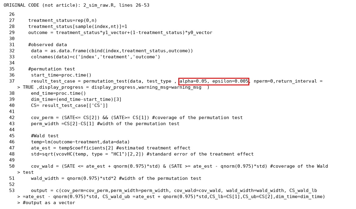
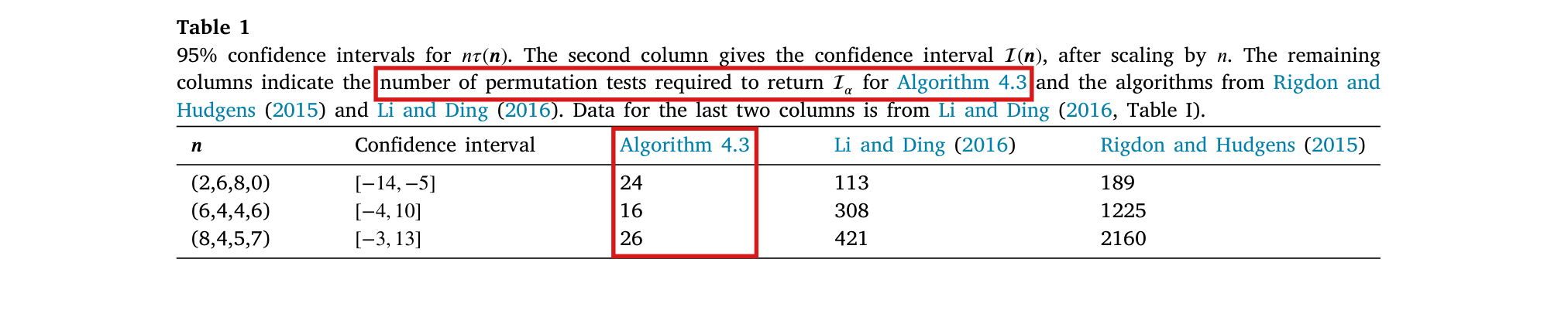
  • Table 1: the three intervals [−14,−5][-14,-5], [−4,10][-4,10] and [−3,13][-3,13] are reproduced exactly, and the counts 189, 1225 and 2160 for the Rigdon–Hudgens method equal the size of the imputation grid. The counts for Algorithm 4.3 are the subject of P003-N007. In the released Monte Carlo code at K=100000K=100000, I obtain [−2,13][-2,13] and 31–32 tests in row 3, versus [−3,13][-3,13] and 26 printed; a tie-tolerance sensitivity gives the printed interval and count.
  • Lemma B.14 and the arithmetic leading to (1.5), (1.6) and (4.9). The statements of Lemma B.15 and of Proposition 4.6 follow by an argument other than the printed one (P003-E003).
  • Remark 5.2: the pp-value SS of (5.3) is valid for every KK. The update (5.21)–(5.26) turns a uniform assignment for v\mathbf v into a uniform assignment for v′\mathbf v'. Theorem 5.5 holds for Algorithm 5.3 with the loop restored as in P003-E002.
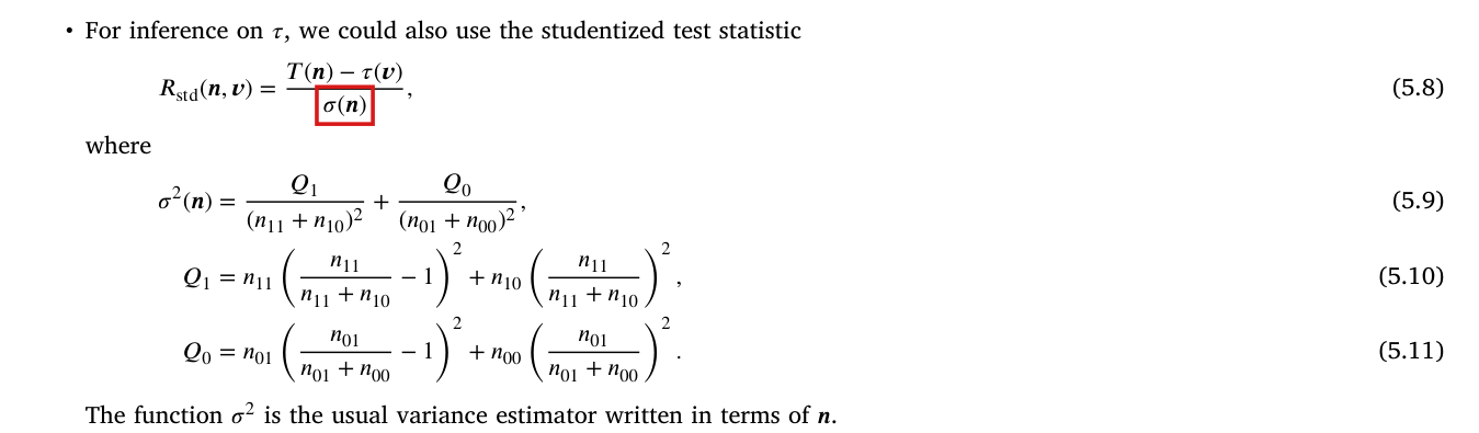
  • The estimands and statistics (5.7)–(5.15), where their denominators are not zero (P003-E005, P003-E011).
  • Proposition 6.2 for balanced designs, and Remark 6.3 (P003-E004). Remark 6.4: the exact coverage is at least 1−α1-\alpha for every table with n0=3,5,…,17n_0=3,5,\ldots,17.
  • The Wald columns of Tables 2 and 3: 13 of the 14 rows that were recomputed exactly agree to within 0.010.01, including the coverage of 0.890.89 quoted in Section 7.1. The exception is the row of P003-E016.
  • The shares of the potential outcomes in the two scenarios sum to one and imply an average effect of zero in Tables 2–7. The number of Monte Carlo draws in the released code matches (4.9).
  • Runs of the released routines at n=50n=50: the coverage entries of Table 3 agree to rounding for all three methods, and the permutation coverage of Table 2 agrees within Monte Carlo error. In Table 2 the permutation median lengths are 0.460.46 against 0.370.37 printed in the first scenario and 0.360.36 against 0.340.34 in the second; these reduced runs do not recover the original simulation outputs. In Table 3, scenario 1, the difference-in-means median length is 0.460.46 against 0.480.48 printed, and the Wald median length is 0.57520.5752 against 0.570.57 printed.
  • Mean widths from the released routines at n=50n=50, compared with Tables 6 and 7: the balanced values are 0.46960.4696 and 0.360.36 against 0.500.50 and 0.350.35 printed. In Table 6 the five unbalanced-algorithm values are about 0.4600.460–0.4650.465 against 0.480.48–0.490.49; in Table 7 they agree to rounding (0.34780.3478 against 0.350.35). These reduced runs do not identify the original outputs behind the printed widths.
  • The attributions to Li and Ding (2016), Rigdon and Hudgens (2015) and Harrison (2012), compared with a preprint or an author manuscript of each: the counts 113, 308, 421 and 189, 1225, 2160 of Table 1, Lemmas 2.4 and 2.5, the pp-value of Remark 5.2 and the O(n4)O(n^4) count of tests.

I did not check the following. The simulations behind Tables 2–7 were not run again at full scale. I retimed the routines behind Tables 4 and 5 only at n=50n=50, on different hardware with four independent weighted blocks; I did not compare absolute times on the original hardware or reproduce the speed crossover. I did not rerun the permutation routines at n=500n=500 or n=1000n=1000, or the permutation columns of Table 3 at n=100n=100 or n=200n=200. The software environment and the hardware of the original runs were not available. The journal editions of the cited works were not compared with the paper, and equation (6.3) of Imbens and Rubin (2015) and the formula of Copas (1973) were not checked.

Three things are missing from the sources. The replication files contain no simulation outputs, and the entries of Tables 2–7 cannot be traced to saved runs. They contain no script for Table 1. One script that their README names, for the second scenario of the unbalanced case at n=1000n=1000, is absent.

These checks do not show that the paper is correct in the respects that were not examined.

Headline claims and related corrections

  1. The intervals obtained by inverting two-sided randomization tests over possible binary potential-outcome tables (the Rigdon-Hudgens intervals) contain the sample average treatment effect with probability at least 1−α1-\alpha for every sample size and allocation with 0<m<n0<m<n.

    Proposition 3.2; Algorithm 2.3; footnote 4

    See P003-E010, P003-N002.

  2. The interval contains the Neyman estimate in balanced designs, though not always in unbalanced designs, and its length is at most of order n−1/2n^{-1/2} when the treated fraction stays bounded away from 00 and 11.

    Lemma 3.1; Proposition 3.3, (3.3); footnote 9; Appendix A.3

    See P003-E019.

  3. In a balanced experiment with n=2mn=2m and n≥15n\ge15, the interval can be constructed with at most 4nlog⁡2n4n\log_2 n permutation tests by binary search over τ0\tau_0, using a monotonicity property of the permutation pp-value; the number of tests is O(nlog⁡n)O(n\log n).

    Theorem 4.1; Lemma 4.2; Algorithm 4.3; Algorithm B.1; Lemmas B.2-B.13; Table 1

    See P003-E001, P003-E006, P003-E007, P003-E008, P003-E009, P003-E013, P003-E015, P003-N007, P003-N018.

  4. For balanced experiments with n≥15n\ge15 and 0<ε<α0<\varepsilon<\alpha, Algorithm 4.5 at level α−ε\alpha-\varepsilon covers τ(y)\tau(\mathbf y) with probability at least 1−α1-\alpha if K≥log⁡(4nlog⁡2(n)/ε)/(2ε2)K\ge\log(4n\log_2(n)/\varepsilon)/(2\varepsilon^2). The Monte Carlo interval can approximate the exact interval arbitrarily well, at total operation cost O((n2log⁡n/ε2)log⁡(nlog⁡n/ε))O((n^2\log n/\varepsilon^2)\log(n\log n/\varepsilon)).

    Proposition 4.6; Lemmas B.14, B.15; Algorithms 4.4, 4.5; (1.5)-(1.6), (4.9)

    See P003-E001, P003-E003, P003-E012, P003-E013, P003-E026, P003-N005.

  5. For general allocations and estimands, including the sample average treatment effect, risk ratio and odds ratio, the Monte Carlo procedure that reuses permutation draws along lines of count vectors returns a confidence set valid for every KK, at cost O(Kn3)O(Kn^3), equivalent to O(n2)O(n^2) Monte Carlo tests rather than O(n4)O(n^4).

    Theorem 5.5; Algorithms 5.1, 5.3; Section 5.1.1; Remarks 5.2, 5.6

    See P003-E002, P003-E005, P003-E011, P003-E022, P003-E023, P003-E024, P003-E025, P003-N001, P003-N020.

  6. The construction extends to experiments with missing outcomes without an assumption on the missingness mechanism: the interval built from the two extremal imputations covers τ(y)\tau(\mathbf y) with probability at least 1−α1-\alpha.

    Proposition 6.2; Definition 6.1; Remarks 6.3, 6.4; Appendix D

    See P003-E004, P003-E015.

  7. The simulations report nominal coverage for the permutation intervals where Wald intervals undercover, including Wald coverage of 89%89\% at n=50n=50 with sparse outcomes, and interval lengths comparable to, and sometimes shorter than, Wald intervals.

    Tables 2 and 3; Section 7.1

    See P003-E011, P003-E016, P003-E021, P003-E022, P003-E023, P003-E024, P003-E025, P003-E026, P003-E027, P003-E028, P003-N012, P003-N014.

  8. Algorithm 4.3 uses fewer permutation tests than the Li-Ding and Rigdon-Hudgens constructions in Table 1. The reported timings favor the unbalanced algorithm at n=50,100,200n=50,100,200 and typically favor the balanced algorithm at n=500,1000n=500,1000 with K≥5000K\ge5000, motivating a recommended switch in the low hundreds.

    Table 1; Tables 4-7; Remark 5.7; Sections 7.1-7.2

    See P003-E013, P003-E017, P003-E018, P003-E020, P003-E021, P003-E022, P003-E023, P003-E028, P003-E030, P003-N007, P003-N011.

  9. The best known preceding constructions required O(n2)O(n^2) tests in balanced designs (Li and Ding, 2016) and O(n4)O(n^4) tests in general (Rigdon and Hudgens, 2015); the Li-Ding algorithm was not proved to return the Rigdon-Hudgens interval in unbalanced designs.

    Lemma 2.4 (Li-Ding Theorem 1); Lemma 2.5 (Li-Ding Theorem A.4); Table 1, last two columns

Corrections

Moderate (8)

A real substantive error with limited reach.

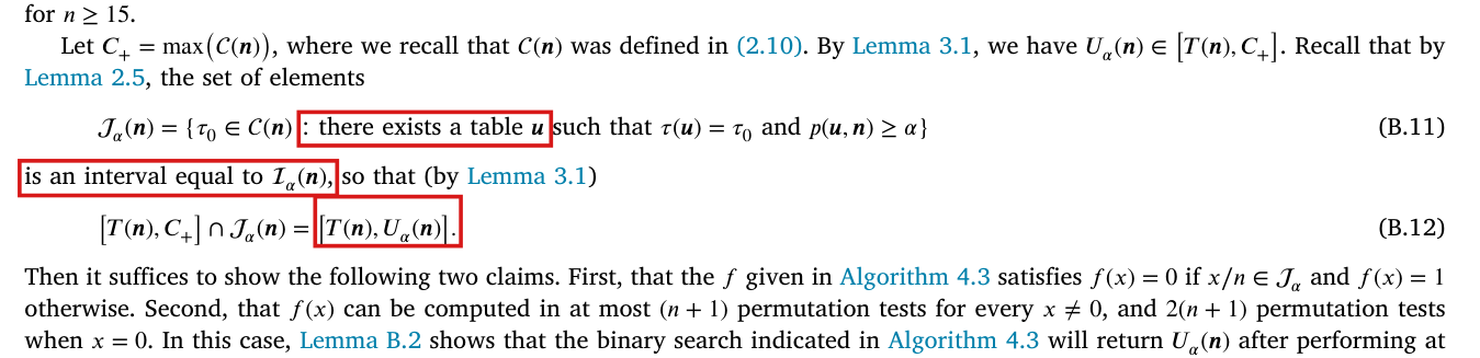
Algorithm B.1 returns k1k_1 in place of k2k_2 on a two-point range where ff is zero, can fail to stop on a two-point range, and excludes ranges that Algorithm 4.3 supplies; the search should start from the points k1−1k_1-1 and k2+1k_2+1, which are never evaluated.

Appendix B.1, Algorithm B.1 (Steps 2 and 3) and Lemma B.2, p. 20 (PDF p. 20); the search is invoked by Algorithm 4.3, p. 8, and in the proof of Theorem 4.1, p. 21

See also under Formal statements (Lean): P003-T4, P003-T5, P003-T7, P003-T23, P003-T27, P003-T32, P003-T34

As printed

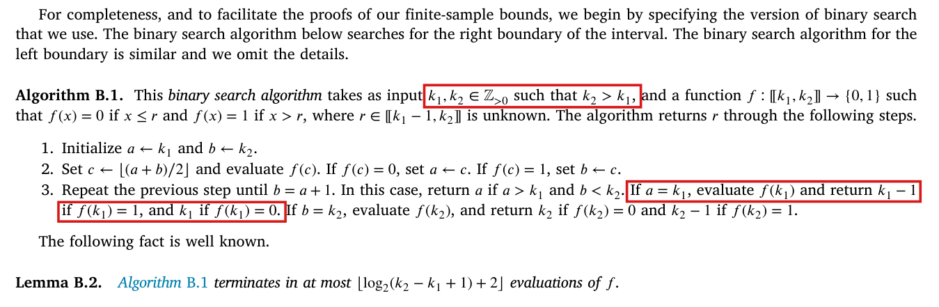
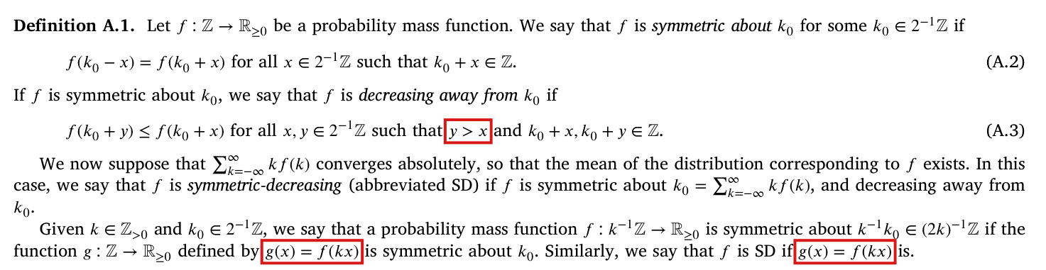
“Algorithm B.1. This binary search algorithm takes as input k1,k2∈Z>0k_1,k_2\in\colorbox{#ffe58a}{$\mathbb Z_{>0}$} such that k2>k1k_2\colorbox{#ffe58a}{$>$}k_1, and a function f:[ ⁣[k1,k2] ⁣]→{0,1}f:[\![k_1,k_2]\!]\to\{0,1\} such that f(x)=0f(x)=0 if x≤rx\le r and f(x)=1f(x)=1 if x>rx>r, where r∈[ ⁣[k1−1,k2] ⁣]r\in[\![k_1-1,k_2]\!] is unknown. The algorithm returns rr through the following steps.

  1. Initialize a←k1a\leftarrow\colorbox{#ffe58a}{$k_1$} and b←k2b\leftarrow\colorbox{#ffe58a}{$k_2$}.
  2. Set c←⌊(a+b)/2⌋c\leftarrow\lfloor(a+b)/2\rfloor and evaluate f(c)f(c). If f(c)=0f(c)=0, set a←ca\leftarrow c. If f(c)=1f(c)=1, set b←cb\leftarrow c.
  3. Repeat the previous step until b=a+1b=a+1. In this case, return aa if a>k1a>k_1 and b<k2b<k_2. If a=k1a=k_1, evaluate f(k1)f(k_1) and return k1−1k_1-1 if f(k1)=1f(k_1)=1, and k1\colorbox{#ffe58a}{$k_1$} if f(k1)=0f(k_1)=0. If b=k2b=k_2, evaluate f(k2)f(k_2), and return k2k_2 if f(k2)=0f(k_2)=0 and k2−1k_2-1 if f(k2)=1f(k_2)=1.

The following fact is well known.

Lemma B.2. Algorithm B.1 terminates in at most ⌊log⁡2(k2−k1+1)+2⌋\colorbox{#ffe58a}{$\lfloor\log_2(k_2-k_1+1)+2\rfloor$} evaluations of ff.”

The problem

Algorithm 4.3 defines its upper endpoint through this search (“The precise definition of this binary search is given as Algorithm B.1”), and the printed steps are part of the algorithm. The steps fail on a range with two points. Suppose that k2=k1+1k_2=k_1+1. Step 2 evaluates ff at c=k1c=k_1. If f(k1)=0f(k_1)=0, then a=k1a=k_1 and b=k2=a+1b=k_2=a+1, and both end conditions of Step 3 hold. The clause for a=k1a=k_1 comes first and returns k1k_1 without evaluating f(k2)f(k_2), which is wrong when f(k2)=0f(k_2)=0, that is, when r=k2r=k_2. If f(k1)=1f(k_1)=1, then Step 2 sets b=k1b=k_1, the pair (a,b)=(k1,k1)(a,b)=(k_1,k_1) repeats, and the condition b=a+1b=a+1 never holds. The search does not stop, which contradicts Lemma B.2. Both inputs satisfy the stated conditions.

The stated conditions also exclude ranges that Algorithm 4.3 passes to the search. Its range is [ ⁣[nT(n),nmax⁡C(n)] ⁣][\![nT(\mathbf n),n\max\mathcal C(\mathbf n)]\!]. The left endpoint can be zero or negative (it is −12-12 in the first row of Table 1), and the range is the single point {n}\{n\} when n11=mn_{11}=m and n01=0n_{01}=0. In a balanced design the range of the upper search is [ ⁣[2(n11−n01), n11−n01+m] ⁣][\![2(n_{11}-n_{01}),\,n_{11}-n_{01}+m]\!]. It has two points exactly when n11−n01=m−1n_{11}-n_{01}=m-1, and then Algorithm 4.3 as printed returns T(n)=(m−1)/mT(\mathbf n)=(m-1)/m as its upper endpoint, although Uα(n)=(2m−1)/(2m)U_\alpha(\mathbf n)=(2m-1)/(2m) for every α∈(0,1)\alpha\in(0,1). This occurs for every m≥2m\ge2, including the range n≥15n\ge15 of Theorem 4.1.

Evidence an exact counterexample

The evidence is an exact counterexample, computed in integer and rational arithmetic, and a derivation of the corrected search.

Inputs on which the printed search fails. The third row is the upper search of Algorithm 4.3 for n=16n=16, m=8m=8, observed counts n=(7,1,0,8)\mathbf n=(7,1,0,8) and α=1/20\alpha=1/20.
RangeValues of ffPrinted searchRequired value rr
{1,2}\{1,2\}f(1)=f(2)=0f(1)=f(2)=0returns 12
{1,2}\{1,2\}f(1)=f(2)=1f(1)=f(2)=1never returns0
{14,15}\{14,15\}f(14)=f(15)=0f(14)=f(15)=0returns 1415

In the third row, I have T(n)=7/8T(\mathbf n)=7/8 and nmax⁡C(n)=15n\max\mathcal C(\mathbf n)=15, and the range is {14,15}\{14,15\}. The count vector v=(0,15,0,1)\mathbf v=(0,15,0,1) is possible given n\mathbf n and has τ(v)=15/16\tau(\mathbf v)=15/16. Over the 12870 assignments, TT takes the values 7/87/8 and 11, each 6435 times, and both are at distance 1/161/16 from 15/1615/16, which is also the observed distance. I obtain p(v,n)=1p(\mathbf v,\mathbf n)=1 and Uα(n)=15/16U_\alpha(\mathbf n)=15/16. Enumerating all 144 possible count vectors gives Iα(n)=[1/2,15/16]\mathcal I_\alpha(\mathbf n)=[1/2,15/16]. The value 14/16=T(n)14/16=T(\mathbf n) is accepted as well, through the table (0,14,0,2)(0,14,0,2), and I have f(14)=f(15)=0f(14)=f(15)=0. The printed search evaluates f(14)f(14) twice, never evaluates f(15)f(15), and returns 14. The upper endpoint of Algorithm 4.3 as printed is then 14/1614/16. If (0,15,0,1)(0,15,0,1) is the true table, these are the observed counts at 6435 of the 12870 assignments, and at each of them the printed upper endpoint is below the true effect 15/1615/16.

For the corrected search (given under Corrected), let N=k2−k1+1N=k_2-k_1+1. The inequalities k1−1≤a≤r<b≤k2+1k_1-1\le a\le r<b\le k_2+1 hold at the start. If b−a≥2b-a\ge2, then a<c<ba<c<b, and ff is evaluated only at points of [ ⁣[k1,k2] ⁣][\![k_1,k_2]\!]. If f(c)=0f(c)=0, then c≤rc\le r, and if f(c)=1f(c)=1, then r<cr<c. In both cases the update preserves the inequalities. Each update replaces b−ab-a by at most ⌈(b−a)/2⌉\lceil(b-a)/2\rceil, and the search stops with b=a+1b=a+1. Then a≤r<a+1a\le r<a+1, and I obtain r=ar=a. The width b−ab-a is N+1N+1 at the start and at most ⌈(N+1)/2t⌉\lceil(N+1)/2^t\rceil after tt evaluations. Since N+1≤2qN+1\le2^q for q=⌊log⁡2N⌋+1q=\lfloor\log_2N\rfloor+1, the search uses at most ⌊log⁡2N⌋+1\lfloor\log_2N\rfloor+1 evaluations.

What survives

The interval Iα\mathcal I_\alpha, Proposition 3.2, Lemma 4.2 and the compatibility test inside Algorithm 4.3 are unaffected. The corrected search retains the bound in Theorem 4.1. The range has at most n+1n+1 points, an evaluation of ff at a nonzero point costs at most n+1n+1 permutation tests, and the evaluation at 00, which occurs at most once, costs at most 2(n+1)2(n+1). Each endpoint costs at most (n+1)(⌊log⁡2(n+1)⌋+2)≤(n+1)⌊log⁡2(n+1)+3⌋(n+1)(\lfloor\log_2(n+1)\rfloor+2)\le(n+1)\lfloor\log_2(n+1)+3\rfloor tests, and (B.10) implies the bound 4nlog⁡2n4n\log_2n. Algorithm 4.5 inherits the search and needs the same correction (see P003-E003); Algorithm 5.3 does not use it. The replication code treats short ranges differently: it skips the midpoint loop when the range has one or two points and always tests the outer upper bound (see P003-N007). No reported simulation or application number is shown to be affected.

Corrected

“Algorithm B.1. This binary search algorithm takes as input k1,k2∈Zk_1,k_2\in\colorbox{#ffe58a}{$\mathbb Z$} such that k2≥k1k_2\colorbox{#ffe58a}{$\ge$}k_1, and a function f:[ ⁣[k1,k2] ⁣]→{0,1}f:[\![k_1,k_2]\!]\to\{0,1\} such that f(x)=0f(x)=0 if x≤rx\le r and f(x)=1f(x)=1 if x>rx>r, where r∈[ ⁣[k1−1,k2] ⁣]r\in[\![k_1-1,k_2]\!] is unknown. The algorithm returns rr through the following steps.

  1. Initialize a←k1−1a\leftarrow\colorbox{#ffe58a}{$k_1-1$} and b←k2+1b\leftarrow\colorbox{#ffe58a}{$k_2+1$}. The function is never evaluated at these two points.
  2. Set c←⌊(a+b)/2⌋c\leftarrow\lfloor(a+b)/2\rfloor and evaluate f(c)f(c). If f(c)=0f(c)=0, set a←ca\leftarrow c. If f(c)=1f(c)=1, set b←cb\leftarrow c.
  3. Repeat the previous step until b=a+1b=a+1. Then return a\colorbox{#ffe58a}{$a$}.

Lemma B.2. Algorithm B.1 terminates and returns r\colorbox{#ffe58a}{$r$} in at most ⌊log⁡2(k2−k1+1)⌋+1\colorbox{#ffe58a}{$\lfloor\log_2(k_2-k_1+1)\rfloor+1$} evaluations of ff.”

The bound in Lemma B.2 is at most the printed bound ⌊log⁡2(k2−k1+1)+2⌋\lfloor\log_2(k_2-k_1+1)+2\rfloor. The search for the left boundary and the search in Algorithm 4.5 are corrected in the same way.

Crop of Algorithm B.1 with the paragraph before it and Lemma B.2 after it. Three red boxes: the input condition 'k1, k2 in the positive integers such that k2 is greater than k1' in the first line, and, over two lines of Step 3, the sentence 'If a = k1, evaluate f(k1) and return k1 - 1 if f(k1) = 1, and k1 if f(k1) = 0.'
Appendix B.1, Algorithm B.1 and Lemma B.2, p. 20 (PDF p. 20). The marked passages are the input condition and the clause of Step 3 that returns when a=k1a=k_1 without evaluating f(k2)f(k_2).

The proof of Lemma B.15 rests on a false identity between the order of the two upper endpoints and the direction of the first disagreement between the exact and the approximate tests; with the corrected binary search, the bounds of the lemma hold, with the same constants, by a union bound over the tests that the approximate search performs.

Appendix B.5, proof of Lemma B.15, pp. 27–28 (PDF pp. 27–28): the paragraph before (B.81), the display that ends with (B.81) and (B.82), and (B.85)–(B.89)

See also under Formal statements (Lean): P003-T6, P003-T7

As printed

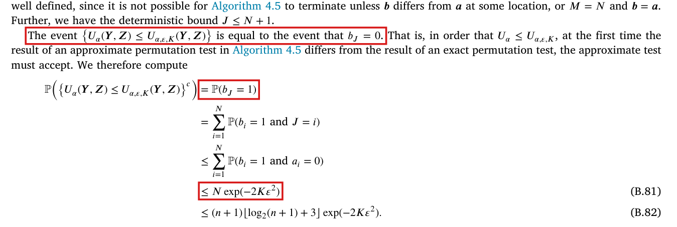
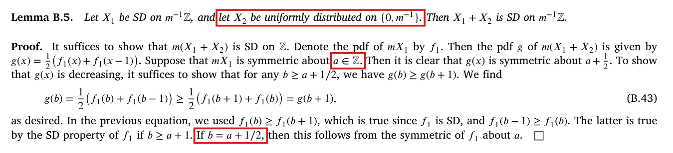
P. 27: “The event {Uα(Y,Z)≤Uα,ε,K(Y,Z)}\{U_\alpha(\mathbf Y,\mathbf Z)\le U_{\alpha,\varepsilon,K}(\mathbf Y,\mathbf Z)\} is equal to the event that bJ=0b_J=0. That is, in order that Uα≤Uα,ε,KU_\alpha\le U_{\alpha,\varepsilon,K}, at the first time the result of an approximate permutation test in Algorithm 4.5 differs from the result of an exact permutation test, the approximate test must accept. We therefore compute

P({Uα(Y,Z)≤Uα,ε,K(Y,Z)}c)=P(bJ=1)=∑i=1NP(bi=1 and J=i)≤∑i=1NP(bi=1 and ai=0)≤Nexp⁡(−2Kε2)(B.81)≤(n+1)⌊log⁡2(n+1)+3⌋exp⁡(−2Kε2).(B.82)”\begin{aligned} \mathbb P\bigl(\{U_\alpha(\mathbf Y,\mathbf Z)\le U_{\alpha,\varepsilon,K}(\mathbf Y,\mathbf Z)\}^c\bigr)&{}\colorbox{#ffe58a}{$\displaystyle =$}\mathbb P(b_J=1)\\ &=\sum_{i=1}^N\mathbb P(b_i=1\text{ and }J=i)\\ &\le\sum_{i=1}^N\mathbb P(b_i=1\text{ and }a_i=0)\\ &{}\colorbox{#ffe58a}{$\displaystyle \le N\exp(-2K\varepsilon^2)$}\qquad\text{(B.81)}\\ &\le(n+1)\lfloor\log_2(n+1)+3\rfloor\exp(-2K\varepsilon^2).\qquad\text{(B.82)''} \end{aligned}

P. 28: “The event {Uα−2ε(Y,Z)≥Uα,ε,K(Y,Z)}\{U_{\alpha-2\varepsilon}(\mathbf Y,\mathbf Z)\ge U_{\alpha,\varepsilon,K}(\mathbf Y,\mathbf Z)\} is equal to the event

{bJ=1}∪{J=N+1}.(B.85)\{b_J=1\}\cup\{J=N+1\}.\qquad\text{(B.85)}

We compute

P({Uα−2ε(Y,Z)≥Uα,ε,K(Y,Z)}c)=P(bJ=0 and J≤N)(B.86)”\mathbb P\bigl(\{U_{\alpha-2\varepsilon}(\mathbf Y,\mathbf Z)\ge U_{\alpha,\varepsilon,K}(\mathbf Y,\mathbf Z)\}^c\bigr)\colorbox{#ffe58a}{$\displaystyle =$}\mathbb P(b_J=0\text{ and }J\le N)\qquad\text{(B.86)''}
The problem

In Algorithm 4.3, the compatibility of one value τ0\tau_0 is decided by testing several tables in turn and stopping at the first acceptance. Algorithm 4.5 does the same with a fresh set of Monte Carlo draws for each table. The sequences a\mathbf a and b\mathbf b record the decisions on single tables, and JJ is the first index at which they differ. The proof asserts that the direction of this first disagreement decides the order of the final upper endpoints. It does not. Suppose that bJ=0b_J=0, that is, the approximate test accepts a table that the exact test rejects. The exact search may accept the next table for the same τ0\tau_0. Both searches then declare τ0\tau_0 compatible and continue from the same midpoint, and a later rejection by the approximate test can still produce Uα,ε,K<UαU_{\alpha,\varepsilon,K}<U_\alpha. In the other direction, a first disagreement with bJ=1b_J=1 can be followed by the acceptance of the next table for the same τ0\tau_0, after which the approximate search can end above the exact endpoint. The identity before (B.81) and the identity (B.85) are therefore false, and so are the equalities of probabilities drawn from them, including (B.86).

The argument has a second error. After the two searches separate, the iith tests of the two sequences can concern different tables. The event {bi=1 and ai=0}\{b_i=1\text{ and }a_i=0\} is then not the rejection of a fixed table whose pp-value is at least α\alpha, Lemma B.14 does not bound its probability, and the bound (B.81) on the sum can fail.

The printed argument therefore does not prove Lemma B.15, and the proof of Proposition 4.6 cites the lemma. The counterexamples to the first-disagreement argument do not refute either probability bound. With the corrected search of P003-E001, both bounds hold with the same constants by the argument given under Evidence. The literal printed search has a separate defect: if an execution that returns no endpoint is assigned the empty interval, then (B.78) fails at v=(0,2,0,0)\mathbf v=(0,2,0,0), m=1m=1, α=3/4\alpha=3/4, ε=1/4\varepsilon=1/4 and K=200K=200. Its inclusion event has probability zero, whereas its claimed lower bound is 1−24e−25≥1/13>01-24e^{-25}\ge1/13>0. Without this convention, the printed interval is undefined at this input. This example does not refute (B.79) or either bound for the corrected search.

Evidence an exact counterexample

I base this finding on an exact counterexample, computed in rational arithmetic, and a derivation of the lemma by a different argument.

Let n=30n=30, m=15m=15, α=1/20\alpha=1/20, ε=1/200\varepsilon=1/200 and K=1K=1, and let the observed counts be n=(2,13,1,14)\mathbf n=(2,13,1,14). With K=1K=1, an approximate test accepts a table with probability equal to its exact pp-value. The upper search runs over the effects x/30x/30 with x∈[ ⁣[2,16] ⁣]x\in[\![2,16]\!], and Uα=Uα−2ε=10/30U_\alpha=U_{\alpha-2\varepsilon}=10/30.

The exact upper search at level α=1/20\alpha=1/20 and one path of the approximate search, which has positive probability.
Effect testedExact searchApproximate search, one path
9/309/30rejects 1 table, accepts (2,9,0,19)(2,9,0,19)accepts (1,9,0,20)(1,9,0,20)
12/3012/30rejects 5 tablesrejects 5 tables
10/3010/30rejects 2 tables, accepts (3,10,0,17)(3,10,0,17)rejects 7 tables
11/3011/30rejects 6 tablesnot tested
Endpoint returned10/3010/309/309/30

At 9/309/30 the exact search rejects (1,9,0,20)(1,9,0,20), whose pp-value is 412/10005<1/20412/10005<1/20, and accepts (2,9,0,19)(2,9,0,19), whose pp-value is 752/10005752/10005. On the path in the table, the approximate search accepts (1,9,0,20)(1,9,0,20), so J=1J=1 and bJ=0b_J=0. It then rejects every table that it tests at 12/3012/30 and at 10/3010/30, including (3,10,0,17)(3,10,0,17), which the exact test accepts with pp-value 7143/1267307143/126730. It returns 9/30<Uα9/30<U_\alpha. The same decisions have positive probability for every KK.

For (B.85), the sequence a\mathbf a is computed at level α−2ε=1/25\alpha-2\varepsilon=1/25, and the first exact test accepts (1,9,0,20)(1,9,0,20). Consider the path on which the approximate search rejects this table, then accepts (2,9,0,19)(2,9,0,19), and then accepts the first table tested at each of 12/3012/30, 14/3014/30, 15/3015/30 and 16/3016/30. On this path J=1J=1 and bJ=1b_J=1, and the search returns 16/30>Uα−2ε16/30>U_{\alpha-2\varepsilon}. The event (B.85) holds, and the event {Uα−2ε≥Uα,ε,K}\{U_{\alpha-2\varepsilon}\ge U_{\alpha,\varepsilon,K}\} does not. Summing over the whole search tree gives the probabilities below.

Probabilities given the observed data in the same example, rounded to four places. The proof equates the first with the second, and the third with the fourth.
EventProbability
Uα,ε,K<UαU_{\alpha,\varepsilon,K}<U_\alpha0.8628
bJ=1b_J=1, with a\mathbf a at level α\alpha0.9489
Uα,ε,K>Uα−2εU_{\alpha,\varepsilon,K}>U_{\alpha-2\varepsilon}0.0300
bJ=0b_J=0 and J≤NJ\le N, with a\mathbf a at level α−2ε\alpha-2\varepsilon0.0038

For (B.81), I keep the data and α\alpha, and set ε=1/50\varepsilon=1/50 and K=5000K=5000. Then N=16N=16 and a2=0a_2=0, and an approximate test accepts when S≥α−ε=3/100S\ge\alpha-\varepsilon=3/100. The pp-value 412/10005412/10005 of (1,9,0,20)(1,9,0,20) is above this threshold. If the first approximate test accepts this table, the second approximate test is the test of (1,12,0,17)(1,12,0,17) at 12/3012/30, whose pp-value 407/190095407/190095 is below the threshold. Applying Chebyshev’s inequality to each of the two tests, I find that P(b2=1 and a2=0)>9/10\mathbb P(b_2=1\text{ and }a_2=0)>9/10, while Nexp⁡(−2Kε2)=16e−4<48/103N\exp(-2K\varepsilon^2)=16e^{-4}<48/103.

For the replacement argument, fix the observed data, and set D=(n+1)⌊log⁡2(n+1)+3⌋D=(n+1)\lfloor\log_2(n+1)+3\rfloor and δ=exp⁡(−2Kε2)\delta=\exp(-2K\varepsilon^2). With the corrected search, the upper search performs at most DD table tests, whatever their outcomes. I number the tests that the approximate search performs. The table Wi\mathbf W_i tested at step ii is determined by the outcomes of the earlier tests, and the draws used at step ii are independent of them. Conditional on the earlier tests, (B.75) implies that a table with p(Wi,n)≥αp(\mathbf W_i,\mathbf n)\ge\alpha is rejected with probability at most δ\delta, and (B.76) implies that a table with p(Wi,n)<α−2εp(\mathbf W_i,\mathbf n)<\alpha-2\varepsilon is accepted with probability at most δ\delta. By a union bound over at most DD steps, each of the following events has probability at least 1−Dδ1-D\delta: no table with pp-value at least α\alpha is rejected, and no table with pp-value below α−2ε\alpha-2\varepsilon is accepted.

On the first event, every value x/n≤Uαx/n\le U_\alpha in the range is declared compatible when it is tested. Indeed, by the proof of Theorem 4.1, the list of tables tested for such a value contains a table with pp-value at least α\alpha, and the approximate search accepts either an earlier table of the list or that one. The upper pointer bb of the search then stays above nUαnU_\alpha, and the search returns Uα,ε,K≥UαU_{\alpha,\varepsilon,K}\ge U_\alpha. On the second event, every table that the approximate search accepts has pp-value at least α−2ε\alpha-2\varepsilon, and every value it declares compatible is at most Uα−2εU_{\alpha-2\varepsilon}. The lower pointer aa then stays at or below nUα−2εnU_{\alpha-2\varepsilon}, and the search returns Uα,ε,K≤Uα−2εU_{\alpha,\varepsilon,K}\le U_{\alpha-2\varepsilon}. The lower endpoints are treated in the same way after every outcome is replaced by its complement, which changes the signs of TT and τ\tau and preserves the pp-values. By a union bound over the two endpoints, each part of Lemma B.15 holds with probability at least 1−2Dδ1-2D\delta.

What survives

Lemma B.15 and Proposition 4.6 hold as stated, with the same constants, when the search is the corrected one and the intervals in their statements are defined (the second part of the lemma needs α−2ε>0\alpha-2\varepsilon>0). This proof error does not affect the statements of Lemma B.14, Lemma 4.2 or Theorem 4.1, or the exact test. The simulations and the application do not use the false identities, and no reported number is shown to be affected.

Corrected

The statement of Lemma B.15 is unchanged. In its proof, replace the passage from “Let NN be the total number of permutation tests” through the sentence following (B.83), ending “which was shown in the proof of Theorem 4.1”, by the following.

“Condition on the observed data, and number the table tests performed by Algorithm 4.5 in the course of finding Uα,ε,K(Y,Z)U_{\alpha,\varepsilon,K}(\mathbf Y,\mathbf Z). There are at most (n+1)⌊log⁡2(n+1)+3⌋(n+1)\lfloor\log_2(n+1)+3\rfloor of them. The table w\mathbf w tested at the iith step is determined by the results of the earlier tests, and Algorithm 4.4 uses new draws at each step. If p(w,Y,Z)≥αp(\mathbf w,\mathbf Y,\mathbf Z)\ge\alpha, then by (B.75), Algorithm 4.4 rejects w\mathbf w with conditional probability at most exp⁡(−2Kε2)\exp(-2K\varepsilon^2). By a union bound, with probability at least

1−(n+1)⌊log⁡2(n+1)+3⌋exp⁡(−2Kε2),1-(n+1)\lfloor\log_2(n+1)+3\rfloor\exp(-2K\varepsilon^2),

Algorithm 4.5 rejects no table w\mathbf w such that p(w,Y,Z)≥αp(\mathbf w,\mathbf Y,\mathbf Z)\ge\alpha. On this event, every τ0≤Uα(Y,Z)\tau_0\le U_\alpha(\mathbf Y,\mathbf Z) that the search tests is declared compatible, and therefore Uα(Y,Z)≤Uα,ε,K(Y,Z)U_\alpha(\mathbf Y,\mathbf Z)\le U_{\alpha,\varepsilon,K}(\mathbf Y,\mathbf Z).”

For the second part, remove the sentence that redefines a\mathbf a and b\mathbf b, and replace the passage from “The event {Uα−2ε(Y,Z)≥Uα,ε,K(Y,Z)}\{U_{\alpha-2\varepsilon}(\mathbf Y,\mathbf Z)\ge U_{\alpha,\varepsilon,K}(\mathbf Y,\mathbf Z)\} is equal to the event” through (B.93) and its justification by the analogous argument. If p(w,Y,Z)<α−2εp(\mathbf w,\mathbf Y,\mathbf Z)<\alpha-2\varepsilon, acceptance implies S−p(w,Y,Z)>εS-p(\mathbf w,\mathbf Y,\mathbf Z)\colorbox{#ffe58a}{$>$}\varepsilon, so (B.76) gives the same conditional bound. Thus, with probability at least 1−(n+1)⌊log⁡2(n+1)+3⌋exp⁡(−2Kε2)1-(n+1)\lfloor\log_2(n+1)+3\rfloor\exp(-2K\varepsilon^2), Algorithm 4.5 accepts no such table, and on this event Uα−2ε(Y,Z)≥Uα,ε,K(Y,Z)U_{\alpha-2\varepsilon}(\mathbf Y,\mathbf Z)\ge U_{\alpha,\varepsilon,K}(\mathbf Y,\mathbf Z). Both passages use the binary search as corrected in P003-E001.

Crop of the paragraph of the proof of Lemma B.15 that begins 'The event {U alpha(Y, Z) is at most U alpha, epsilon, K(Y, Z)} is equal to the event that b_J = 0' and of the display that follows it, which ends with (B.81) and (B.82). Three red boxes: that first sentence; the first equality of the display, '= P(b_J = 1)'; and the line 'at most N exp(-2 K epsilon squared)', numbered (B.81).
Appendix B.5, proof of Lemma B.15, p. 27 (PDF p. 27). The marked passages are the asserted identity of events, the equality of probabilities drawn from it, and the bound (B.81). The same step is repeated at (B.85)–(B.89) on p. 28.

Proposition 6.2 is false as stated: in an unbalanced design, the interval (6.2) can cover τ(y)\tau(\mathbf y) with probability below 1−α1-\alpha. The proposition holds when n=2mn=2m; for general m<nm<n, the interval can be replaced by the hull of the exact intervals over all completions of the missing outcomes.

Proposition 6.2 and equation (6.2) of Definition 6.1, p. 14 (PDF p. 14); Appendix D, displays (D.3) and (D.7), p. 29 (PDF p. 29)

See also under Formal statements (Lean): P003-T1, P003-T2, P003-T3, P003-T26

As printed

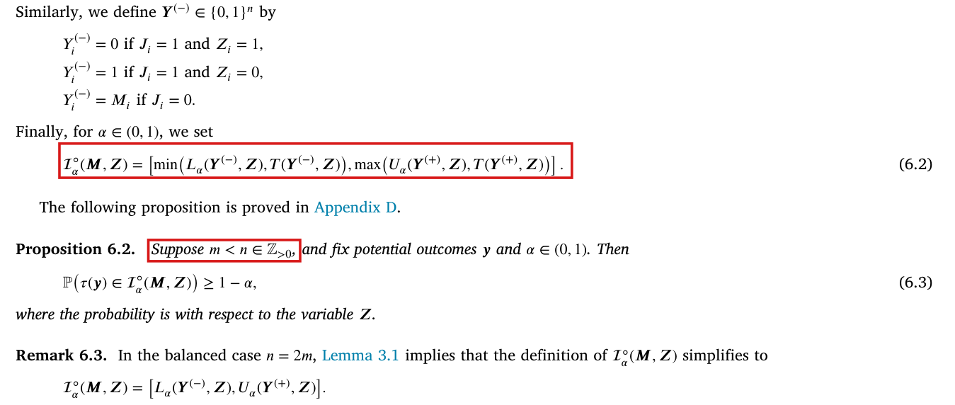
P. 14: “Finally, for α∈(0,1)\alpha\in(0,1), we set

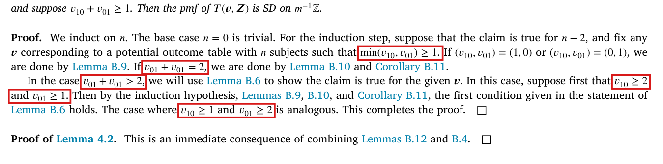
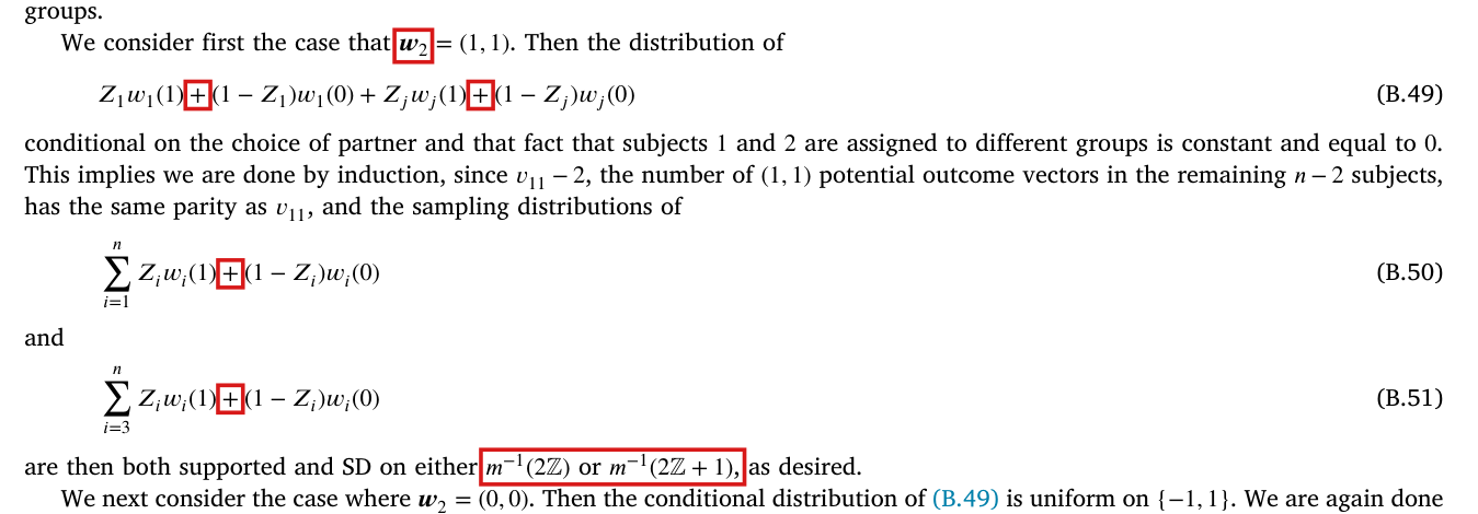
Iα∘(M,Z)=[min⁡(Lα(Y(−),Z),T(Y(−),Z)), max⁡(Uα(Y(+),Z),T(Y(+),Z))].(6.2)\mathcal I^\circ_\alpha(\mathbf M,\mathbf Z)=\Bigl[\colorbox{#ffe58a}{$\displaystyle \min\bigl(L_\alpha(\mathbf Y^{(-)},\mathbf Z),T(\mathbf Y^{(-)},\mathbf Z)\bigr)$},\ \colorbox{#ffe58a}{$\displaystyle \max\bigl(U_\alpha(\mathbf Y^{(+)},\mathbf Z),T(\mathbf Y^{(+)},\mathbf Z)\bigr)$}\Bigr].\qquad\text{(6.2)}

The following proposition is proved in Appendix D.

Proposition 6.2. Suppose m<n∈Z>0\colorbox{#ffe58a}{$m<n\in\mathbb Z_{>0}$}, and fix potential outcomes y\mathbf y and α∈(0,1)\alpha\in(0,1). Then

P(τ(y)∈Iα∘(M,Z))≥1−α,(6.3)\mathbb P\bigl(\tau(\mathbf y)\in\mathcal I^\circ_\alpha(\mathbf M,\mathbf Z)\bigr)\ge1-\alpha,\qquad\text{(6.3)}

where the probability is with respect to the variable Z\mathbf Z.”

P. 29: “First, note that by Proposition 3.2,

P(τ(y)∈Jα(M,Z))≥1−α,(D.1)\mathbb P\bigl(\tau(\mathbf y)\in\mathcal J_\alpha(\mathbf M,\mathbf Z)\bigr)\ge1-\alpha,\qquad\text{(D.1)}

where

Jα(M,Z)=⋃Y′∈Y(M)Iα(Y′,Z),(D.2)\mathcal J_\alpha(\mathbf M,\mathbf Z)=\bigcup_{\mathbf Y'\in\mathcal Y(\mathbf M)}\mathcal I_\alpha(\mathbf Y',\mathbf Z),\qquad\text{(D.2)}

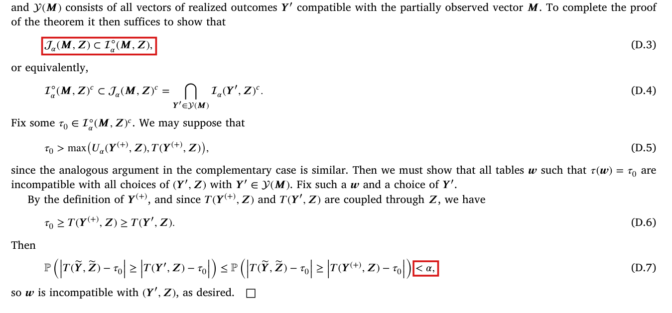
and Y(M)\mathcal Y(\mathbf M) consists of all vectors of realized outcomes Y′\mathbf Y' compatible with the partially observed vector M\mathbf M. To complete the proof of the theorem it then suffices to show that

Jα(M,Z)⊂Iα∘(M,Z),(D.3)\colorbox{#ffe58a}{$\displaystyle \mathcal J_\alpha(\mathbf M,\mathbf Z)\subset\mathcal I^\circ_\alpha(\mathbf M,\mathbf Z)$},\qquad\text{(D.3)}

[…] Fix some τ0∈Iα∘(M,Z)c\tau_0\in\mathcal I^\circ_\alpha(\mathbf M,\mathbf Z)^c. We may suppose that

τ0>max⁡(Uα(Y(+),Z),T(Y(+),Z)),(D.5)\tau_0>\max\bigl(U_\alpha(\mathbf Y^{(+)},\mathbf Z),T(\mathbf Y^{(+)},\mathbf Z)\bigr),\qquad\text{(D.5)}

since the analogous argument in the complementary case is similar. Then we must show that all tables w\mathbf w such that τ(w)=τ0\tau(\mathbf w)=\tau_0 are incompatible with all choices of (Y′,Z)(\mathbf Y',\mathbf Z) with Y′∈Y(M)\mathbf Y'\in\mathcal Y(\mathbf M). Fix such a w\mathbf w and a choice of Y′\mathbf Y'. By the definition of Y(+)\mathbf Y^{(+)}, and since T(Y(+),Z)T(\mathbf Y^{(+)},\mathbf Z) and T(Y′,Z)T(\mathbf Y',\mathbf Z) are coupled through Z\mathbf Z, we have

τ0≥T(Y(+),Z)≥T(Y′,Z).(D.6)\tau_0\ge T(\mathbf Y^{(+)},\mathbf Z)\ge T(\mathbf Y',\mathbf Z).\qquad\text{(D.6)}

Then

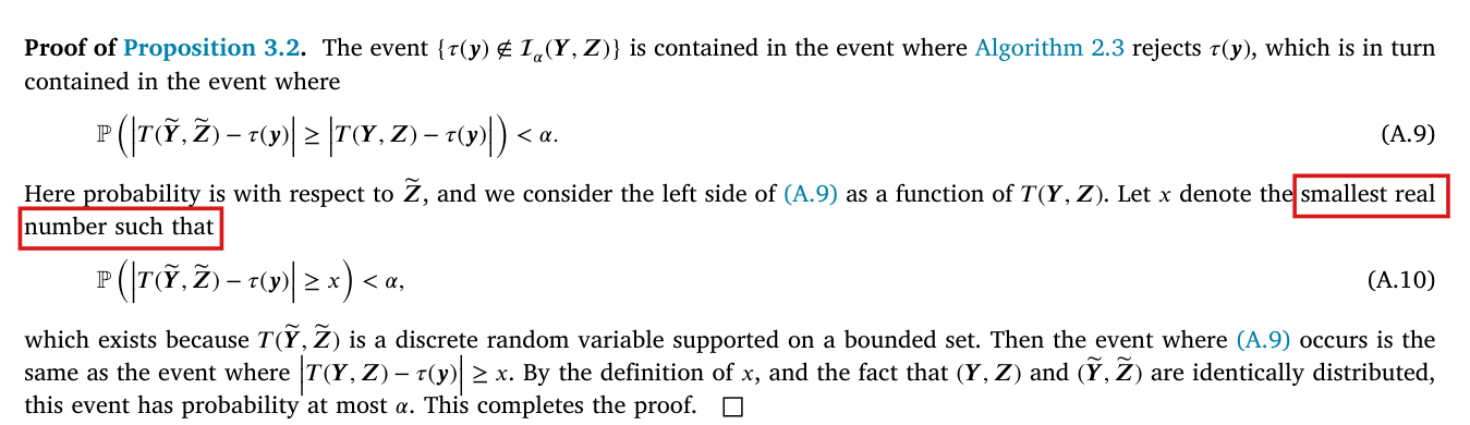
P(∣T(Y~,Z~)−τ0∣≥∣T(Y′,Z)−τ0∣)≤P(∣T(Y~,Z~)−τ0∣≥∣T(Y(+),Z)−τ0∣)<α,(D.7)\mathbb P\Bigl(\bigl|T(\widetilde{\mathbf Y},\widetilde{\mathbf Z})-\tau_0\bigr|\ge\bigl|T(\mathbf Y',\mathbf Z)-\tau_0\bigr|\Bigr)\le\mathbb P\Bigl(\bigl|T(\widetilde{\mathbf Y},\widetilde{\mathbf Z})-\tau_0\bigr|\ge\bigl|T(\mathbf Y^{(+)},\mathbf Z)-\tau_0\bigr|\Bigr)\colorbox{#ffe58a}{$\displaystyle <\alpha$},\qquad\text{(D.7)}

so w\mathbf w is incompatible with (Y′,Z)(\mathbf Y',\mathbf Z), as desired.”

The problem

Proposition 6.2 claims coverage for every allocation m<nm<n and for every distribution allowed in Section 6 for the indicator J\mathbf J of the missing outcomes, which may depend on Y\mathbf Y and Z\mathbf Z. The claim fails in an unbalanced design. In the example given under Evidence, with n=20n=20 and m=3m=3, the interval (6.2) covers τ(y)\tau(\mathbf y) with probability 891/1140891/1140, which is below 1−α=391/5001-\alpha=391/500.

The proof fails at the last inequality of (D.7). I call the vectors Y′∈Y(M)\mathbf Y'\in\mathcal Y(\mathbf M) of (D.2) the completions of M\mathbf M. By (D.5), the value τ0\tau_0 lies above Uα(Y(+),Z)U_\alpha(\mathbf Y^{(+)},\mathbf Z). By Algorithm 2.3, this means that every table with effect τ0\tau_0 that is possible given (Y(+),Z)(\mathbf Y^{(+)},\mathbf Z) has a pp-value below α\alpha. The table w\mathbf w fixed in the proof may be possible given the completion (Y′,Z)(\mathbf Y',\mathbf Z). When Y′≠Y(+)\mathbf Y'\ne\mathbf Y^{(+)}, it need not be possible given (Y(+),Z)(\mathbf Y^{(+)},\mathbf Z), and then (D.5) says nothing about its pp-value. In the example, the true table is possible given the complete data, not possible given the upper imputation, and has the pp-value 249/1140>α249/1140>\alpha for both. The inclusion (D.3) fails as well, since the exact interval of one completion, the complete data, is not contained in (6.2).

The correction changes the missing-outcome extension in Section 6; the complete-data results of Sections 2–5 do not depend on Proposition 6.2. One option is to add the hypothesis n=2mn=2m, under which Proposition 6.2 holds for the interval (6.2), whatever outcomes are missing; the guarantee then does not extend to unbalanced experiments. The other option is to keep general m<nm<n and replace (6.2) by the hull of the exact intervals over all completions. This interval can be wider, and it may require (r1+1)(r0+1)(r_1+1)(r_0+1) interval computations in place of two, where r1r_1 and r0r_0 are the numbers of missing outcomes in the treatment and control groups.

The shortfall in the example is 1/23751/2375, at the level α=109/500\alpha=109/500. No failure at α=0.05\alpha=0.05 or α=0.10\alpha=0.10 is established, nor a smallest example, nor a description of the allocations for which (6.2) fails.

Evidence an exact counterexample

The evidence is an exact counterexample, obtained by enumerating all assignments in integer and rational arithmetic, and derivations of the two corrections.

For the counterexample, let n=20n=20, m=3m=3 and α=109/500\alpha=109/500. Units 1 to 11 have potential outcomes (yi(1),yi(0))=(1,1)(y_i(1),y_i(0))=(1,1), units 12 to 14 have (0,1)(0,1), and units 15 to 20 have (0,0)(0,0). The count vector is (11,0,3,6)(11,0,3,6) and τ(y)=−3/20\tau(\mathbf y)=-3/20. The outcome of unit 1 is missing exactly when the treated units are 12, 13 and 14, and no other outcome is ever missing. This rule depends on Z\mathbf Z only and is allowed by Section 6. There are 1140 assignments. Since 1140α=248.521140\alpha=248.52, a table is accepted when the two-sided tail in (2.12) contains at least 249 assignments.

At the assignment {12,13,14}\{12,13,14\}, the complete data have observed counts (0,3,11,6)(0,3,11,6). Unit 1 is a control with outcome 1. The lower imputation restores this outcome, and the upper imputation replaces it by 0, which gives the counts (0,3,10,7)(0,3,10,7). The exact intervals are Iα=[−7/10,−3/20]\mathcal I_\alpha=[-7/10,-3/20] for the counts (0,3,11,6)(0,3,11,6) and Iα=[−13/20,−1/5]\mathcal I_\alpha=[-13/20,-1/5] for the counts (0,3,10,7)(0,3,10,7). Since T(Y(−),Z)=−11/17T(\mathbf Y^{(-)},\mathbf Z)=-11/17 and T(Y(+),Z)=−10/17T(\mathbf Y^{(+)},\mathbf Z)=-10/17, the interval (6.2) is

[min⁡(−7/10,−11/17),max⁡(−1/5,−10/17)]=[−7/10,−1/5],\bigl[\min(-7/10,-11/17),\max(-1/5,-10/17)\bigr]=[-7/10,-1/5],

which excludes τ(y)=−3/20\tau(\mathbf y)=-3/20. The tail of the true table contains the assignments in which none or all three of the treated units are among units 1 to 11, for both sets of counts, and their number is (93)+(113)=249\binom93+\binom{11}3=249. The true table is possible given the complete data. It is not possible given the upper imputation: since no treated unit has outcome 1, all eleven units of type (1,1)(1,1) are controls and show eleven control outcomes equal to 1, while the upper imputation has ten. Among the tables that are possible given the upper imputation and have effect at least −3/20-3/20, the largest tail count is 248, attained by (8,0,3,9)(8,0,3,9) and (9,0,3,8)(9,0,3,8). With w=y\mathbf w=\mathbf y, τ0=−3/20\tau_0=-3/20 and Y′=Y\mathbf Y'=\mathbf Y, the hypothesis (D.5) holds and both probabilities in (D.7) equal 249/1140>α249/1140>\alpha.

The 1140 assignments of the example, grouped by the observed counts n\mathbf n of the complete data. Tail: number of assignments in the two-sided tail of the true table (accepted if at least 249). Last two columns: number of assignments at which τ(y)=−3/20\tau(\mathbf y)=-3/20 is covered, with complete data and with the interval (6.2) under the rule for the missing outcome.
n\mathbf nAssignmentsTailIα(n)\mathcal I_\alpha(\mathbf n)Complete dataInterval (6.2)
(0,3,11,6)(0,3,11,6)1249[−7/10, −3/20][-7/10,\,-3/20]10
(0,3,12,5)(0,3,12,5)1883[−3/4, −3/10][-3/4,\,-3/10]00
(0,3,13,4)(0,3,13,4)4565[−4/5, −7/20][-4/5,\,-7/20]00
(0,3,14,3)(0,3,14,3)2020[−17/20, −2/5][-17/20,\,-2/5]00
(1,2,11,6)(1,2,11,6)33810[−11/20, 1/20][-11/20,\,1/20]3333
(1,2,12,5)(1,2,12,5)198612[−3/5, 0][-3/5,\,0]198198
(1,2,13,4)(1,2,13,4)165414[−13/20, −1/20][-13/20,\,-1/20]165165
(2,1,11,6)(2,1,11,6)165777[−7/20, 1/4][-7/20,\,1/4]165165
(2,1,12,5)(2,1,12,5)3301140[−2/5, 1/5][-2/5,\,1/5]330330
(3,0,11,6)(3,0,11,6)165248[−1/10, 2/5][-1/10,\,2/5]00
Total1140892891

With complete data, τ(y)\tau(\mathbf y) is covered at 892 assignments. The missing outcome changes the interval at one assignment, and the interval (6.2) covers at 891. The coverage is 891/1140=297/380891/1140=297/380, and 391/500−297/380=1/2375>0391/500-297/380=1/2375>0.

For the balanced case, suppose that n=2mn=2m. Fix an assignment, a pattern of missing outcomes, a completion Y′\mathbf Y', and a table w\mathbf w that is possible given (Y′,Z)(\mathbf Y',\mathbf Z) with p(w,Y′,Z)≥αp(\mathbf w,\mathbf Y',\mathbf Z)\ge\alpha. Set τ0=τ(w)\tau_0=\tau(\mathbf w). If τ0≤T(Y(+),Z)\tau_0\le T(\mathbf Y^{(+)},\mathbf Z), then τ0\tau_0 does not exceed the upper endpoint of (6.2). Otherwise, let dd be the number of units at which Y′\mathbf Y' and Y(+)\mathbf Y^{(+)} differ; their outcomes are missing. Define w+\mathbf w^+ from w\mathbf w by replacing wi(Zi)w_i(Z_i) by Yi(+)Y^{(+)}_i at each of these units. Then w+\mathbf w^+ is possible given (Y(+),Z)(\mathbf Y^{(+)},\mathbf Z). Each replacement raises the effect of its unit by 1 and raises TT by 1/m=2/n1/m=2/n. I have τ(w+)=τ0+d/n\tau(\mathbf w^+)=\tau_0+d/n and T(Y(+),Z)=T(Y′,Z)+2d/nT(\mathbf Y^{(+)},\mathbf Z)=T(\mathbf Y',\mathbf Z)+2d/n. For an assignment z\mathbf z, let N(z)N(\mathbf z) be the number of replaced entries that are realized under z\mathbf z. Then 0≤N(z)≤d0\le N(\mathbf z)\le d and T(w+,z)=T(w,z)+2N(z)/nT(\mathbf w^+,\mathbf z)=T(\mathbf w,\mathbf z)+2N(\mathbf z)/n, and I obtain

∣(T(w+,z)−τ(w+))−(T(w,z)−τ0)∣=∣2N(z)−d∣n≤dn.\bigl|\bigl(T(\mathbf w^+,\mathbf z)-\tau(\mathbf w^+)\bigr)-\bigl(T(\mathbf w,\mathbf z)-\tau_0\bigr)\bigr|=\frac{|2N(\mathbf z)-d|}{n}\le\frac dn.

Set Δ=τ0−T(Y′,Z)\Delta=\tau_0-T(\mathbf Y',\mathbf Z), which satisfies Δ>2d/n\Delta>2d/n. The observed distance is Δ\Delta for w\mathbf w and Δ−d/n\Delta-d/n for w+\mathbf w^+. If ∣T(w,z)−τ0∣≥Δ|T(\mathbf w,\mathbf z)-\tau_0|\ge\Delta, then ∣T(w+,z)−τ(w+)∣≥Δ−d/n|T(\mathbf w^+,\mathbf z)-\tau(\mathbf w^+)|\ge\Delta-d/n. The tail of w\mathbf w is contained in the tail of w+\mathbf w^+, and I find that p(w+,Y(+),Z)≥p(w,Y′,Z)≥αp(\mathbf w^+,\mathbf Y^{(+)},\mathbf Z)\ge p(\mathbf w,\mathbf Y',\mathbf Z)\ge\alpha. Since w+\mathbf w^+ is possible and accepted, Algorithm 2.3 implies that Uα(Y(+),Z)≥τ(w+)≥τ0U_\alpha(\mathbf Y^{(+)},\mathbf Z)\ge\tau(\mathbf w^+)\ge\tau_0. The lower endpoint is treated in the same way after every outcome and potential outcome is replaced by its complement. I conclude that (D.3) holds when n=2mn=2m, and (D.1) then implies (6.3).

For general m<nm<n, the complete vector Y\mathbf Y is one of the completions of M\mathbf M at every assignment, whatever outcomes are missing. The interval Iα(Y,Z)\mathcal I_\alpha(\mathbf Y,\mathbf Z) is then contained in the hull over all completions, and the coverage follows from Proposition 3.2. In the example, the hull at the assignment {12,13,14}\{12,13,14\} is [−7/10,−3/20][-7/10,-3/20], and the hull covers τ(y)\tau(\mathbf y) at 892 assignments. If r1r_1 treated and r0r_0 control outcomes are missing, the exact interval of a completion depends only on how many missing outcomes in each group are set to 1, and there are (r1+1)(r0+1)(r_1+1)(r_0+1) such choices.

What survives

Display (D.1) and the union (D.2) stand: the union of the exact intervals over all completions covers τ(y)\tau(\mathbf y) with probability at least 1−α1-\alpha, and so does its hull. For balanced designs, Proposition 6.2 holds with the interval (6.2), and Remark 6.3 stands. Sections 2 to 5 and the comparisons of Section 7 use complete data and do not depend on Proposition 6.2. The guarantee for the interval (6.2) in unbalanced designs is lost. Remark 6.4 has a different target, the effect in the original 2m−12m-1 subjects, and the example neither proves nor refutes it.

Corrected

Either of the following two statements is correct. The first keeps the interval (6.2) and restricts the design.

“Proposition 6.2. Suppose n=2m\colorbox{#ffe58a}{$n=2m$} for some m∈Z>0\colorbox{#ffe58a}{$m\in\mathbb Z_{>0}$}, and fix potential outcomes y\mathbf y and α∈(0,1)\alpha\in(0,1). Then

P(τ(y)∈Iα∘(M,Z))≥1−α,(6.3)\mathbb P\bigl(\tau(\mathbf y)\in\mathcal I^\circ_\alpha(\mathbf M,\mathbf Z)\bigr)\ge1-\alpha,\qquad\text{(6.3)}

where the probability is with respect to the variable Z\mathbf Z.”

Here J\mathbf J may have any distribution and may depend on Y\mathbf Y and Z\mathbf Z, as in Section 6. In Appendix D, the argument after (D.3) is replaced by the argument for the balanced case given under Evidence.

The second keeps every m<nm<n and changes the interval in Definition 6.1.

“Finally, for α∈(0,1)\alpha\in(0,1), we set

Iα∘(M,Z)=[min⁡Y′∈Y(M)Lα(Y′,Z), max⁡Y′∈Y(M)Uα(Y′,Z)],(6.2)\mathcal I^\circ_\alpha(\mathbf M,\mathbf Z)=\Bigl[\colorbox{#ffe58a}{$\displaystyle \min_{\mathbf Y'\in\mathcal Y(\mathbf M)}L_\alpha(\mathbf Y',\mathbf Z)$},\ \colorbox{#ffe58a}{$\displaystyle \max_{\mathbf Y'\in\mathcal Y(\mathbf M)}U_\alpha(\mathbf Y',\mathbf Z)$}\Bigr],\qquad\text{(6.2)}

where Y(M)\mathcal Y(\mathbf M) is the set of vectors in {0,1}n\{0,1\}^n that agree with M\mathbf M at every observed entry.”

With this definition, Proposition 6.2 holds as printed for every m<nm<n, and its proof ends at (D.2): the interval contains Jα(M,Z)\mathcal J_\alpha(\mathbf M,\mathbf Z), and (D.1) gives (6.3).

Crop of the second half of the proof of Proposition 6.2, with displays (D.3) to (D.7). Two red boxes: display (D.3), 'J alpha(M, Z) is a subset of I circle alpha(M, Z)', and the final 'less than alpha' at the end of display (D.7), which bounds a probability involving T(Y(+), Z). The last line reads 'so w is incompatible with (Y prime, Z), as desired.'
Appendix D, proof of Proposition 6.2, p. 29 (PDF p. 29), from (D.3) to the end. The marked passages are the inclusion (D.3), which fails in the example below, and the last inequality of (D.7), which does not follow from (D.5) when w\mathbf w is not possible given (Y(+),Z)(\mathbf Y^{(+)},\mathbf Z).
Crop of the end of Definition 6.1, Proposition 6.2 and Remark 6.3. Two red boxes: display (6.2), which defines I circle alpha(M, Z) as the interval from min(L alpha(Y(-), Z), T(Y(-), Z)) to max(U alpha(Y(+), Z), T(Y(+), Z)); and the words 'Suppose m less than n in the positive integers,' at the start of Proposition 6.2, whose display (6.3) states that the interval contains tau(y) with probability at least 1 - alpha.
Definition 6.1, Proposition 6.2 and Remark 6.3, p. 14 (PDF p. 14). The marked passages are the interval (6.2), built from the two extremal imputations, and the hypothesis of Proposition 6.2, which allows every m<nm<n.
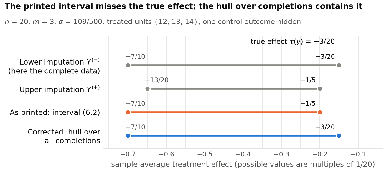
Chart with a horizontal axis for the sample average treatment effect, with labelled ticks from -0.7 to -0.1, and four horizontal intervals. Lower imputation, which here equals the complete data: from -7/10 to -3/20, in grey. Upper imputation: from -13/20 to -1/5, in grey. As printed, interval (6.2): from -7/10 to -1/5, in orange. Corrected, hull over all completions: from -7/10 to -3/20, in blue. A vertical line marks the true effect -3/20. The printed interval stops one step of 1/20 short of the line, and the corrected interval ends on it.
The intervals at the one assignment of the example at which an outcome is hidden (n=20n=20, m=3m=3, α=109/500\alpha=109/500, treated units 12, 13, 14). The interval (6.2) as printed is [−7/10,−1/5][-7/10,-1/5] and excludes the true effect −3/20-3/20; the hull over the completions is [−7/10,−3/20][-7/10,-3/20].

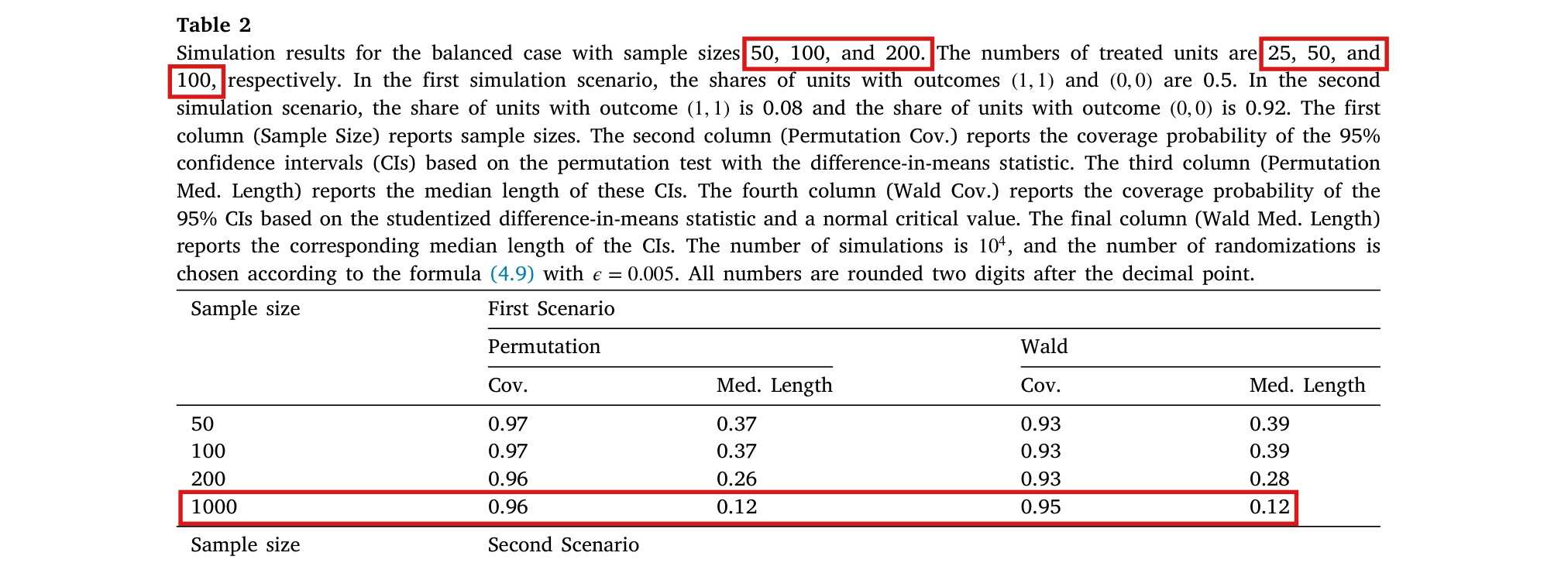
The first-scenario row of Table 2 for n=50n=50 repeats the row for n=100n=100, and its Wald coverage 0.93 and Wald median length 0.39 cannot both come from the stated 50-unit design; the row has to be recomputed from recovered or regenerated 50-unit outputs.

Table 2, first scenario, row for sample size 50, p. 15 (PDF p. 15)

See also under Formal statements (Lean): P003-T8

As printed
Table 2, first scenario, first two rows.
Sample sizeFirst Scenario
PermutationWald
Cov.Med. LengthCov.Med. Length
500.970.370.930.39
1000.970.370.930.39
The problem

The row for sample size 50 in the first scenario prints the same four values as the row for sample size 100. The caption fixes the design behind the row: 50 units, of which 25 have potential outcomes (1,1)(1,1) and 25 have (0,0)(0,0), with 25 units treated. The sample average treatment effect is 0. In this design the data depend on the assignment only through the number kk of treated units with potential outcomes (1,1)(1,1), and the 95% Wald interval covers 0 only when 10≤k≤1510\le k\le 15. Each of these intervals has length at least 0.5540.554. A coverage that rounds to 0.93 implies that more than half of the simulated intervals cover 0. Their median length is then at least 0.5540.554, and it cannot round to 0.39. At least one of the two Wald entries is wrong, whatever the random seed and the number of simulations. For the stated design the exact coverage is 0.91130.9113 and the exact median length is 0.56170.5617. The printed pair agrees with the exact values for n=100n=100, which are 0.92870.9287 and 0.39470.3947.

Evidence an exact counterexample

The evidence is an exact computation over all assignments of the stated design, with an independent calculation in R that uses the regression and the HC1 variance of the replication code. Let kk be the number of treated units with potential outcomes (1,1)(1,1). Then

P(k)=(25k)(2525−k)(5025),τ^k=2k−2525,k=0,…,25.P(k)=\frac{\binom{25}{k}\binom{25}{25-k}}{\binom{50}{25}},\qquad \widehat\tau_k=\frac{2k-25}{25},\qquad k=0,\ldots,25.

The proportions of ones in the two arms are p1=k/25p_1=k/25 and p0=(25−k)/25p_0=(25-k)/25, and the HC1 variance estimate is

Vk=5048{p1(1−p1)25+p0(1−p0)25}=k(25−k)7500.V_k=\frac{50}{48}\left\{\frac{p_1(1-p_1)}{25}+\frac{p_0(1-p_0)}{25}\right\}=\frac{k(25-k)}{7500}.

Let z=Φ−1(0.975)z=\Phi^{-1}(0.975); then 1.95996398454005<z<1.959963984540061.95996398454005<z<1.95996398454006. The interval τ^k±zVk\widehat\tau_k\pm z\sqrt{V_k} has length wk=2zVkw_k=2z\sqrt{V_k}, and it covers 0 exactly when τ^k2≤z2Vk\widehat\tau_k^2\le z^2V_k. With d=2k−25d=2k-25, this condition reads 48d2≤z2(625−d2)48d^2\le z^2(625-d^2). It holds for ∣d∣≤5|d|\le 5 and fails for ∣d∣≥7|d|\ge 7. Since dd is odd, I conclude that the interval covers 0 exactly when 10≤k≤1510\le k\le 15. For these kk, I have k(25−k)≥150k(25-k)\ge 150 and Vk≥1/50V_k\ge 1/50, which gives

wk≥2z1/50≈0.5544.w_k\ge 2z\sqrt{1/50}\approx 0.5544.

Consider any finite set of runs whose coverage rounds to 0.93. More than half of its intervals cover 0. Then the middle length, or each of the two middle lengths when the number of runs is even, is at least 2z1/502z\sqrt{1/50}, and so is the median. A median printed as 0.39 is at most 0.3950.395, which is a contradiction. Summing P(k)P(k) over 10≤k≤1510\le k\le 15, I obtain the exact coverage

1439908169690015801325804719≈0.9113,\frac{14399081696900}{15801325804719}\approx 0.9113,

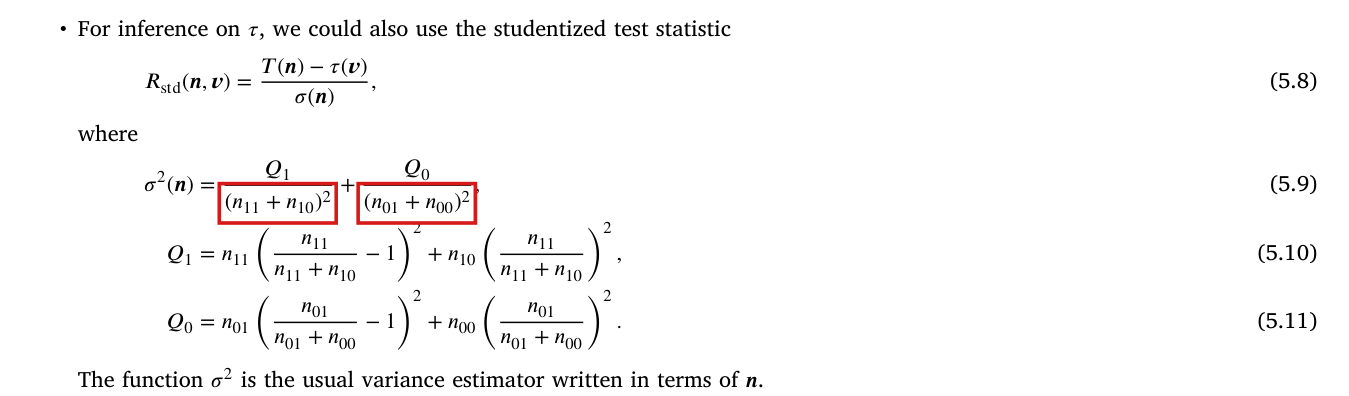
and the median of wkw_k under PP is 2z77/3750≈0.56172z\sqrt{77/3750}\approx 0.5617, attained at k=11k=11 and k=14k=14. The same argument applies to the variance printed in (5.9)–(5.11), which omits the factor 50/4850/48: the interval covers 0 for the same values of kk, and every such interval has length at least 2z12/625≈0.54322z\sqrt{12/625}\approx 0.5432.

Wald columns of Table 2, first scenario: printed values and exact values for the stated designs.
Sample sizeCov., printedCov., exactMed. length, printedMed. length, exact
500.930.91130.390.5617
1000.930.92870.390.3947
What survives

The algorithms, their proofs and the coverage and complexity results do not use this row. This finding does not concern the other rows of Table 2, the sparse-outcome example of Section 7.1 (reported coverage 89% at n=50n=50 in the second scenario) or the timing tables; I have not examined those results here. Section 7.1 uses Table 2 to compare the two methods, and this row must be corrected before it is used for a quantitative comparison. The two permutation entries of the row also repeat the row for n=100n=100. In a reduced run of the released balanced routine for the stated 50-unit design, with exact assignment weights and four independent Monte Carlo blocks, I obtain coverage 0.97730.9773 and median length 0.460.46, against 0.970.97 and 0.370.37 printed. These results describe the released routine; they do not recover the original simulation outputs and are not replacement values for the table.

Corrected

Table 2, first scenario, n=50n=50: the printed row repeats the values for n=100n=100 and is incompatible with the stated 50-unit experiment. The row is to be recomputed from recovered or regenerated outputs for n=50n=50, with the Wald coverage and the Wald median length computed from the same intervals, and the two permutation entries checked against the same outputs.

For the stated design (50 units, 25 with potential outcomes (1,1)(1,1) and 25 with (0,0)(0,0), 25 units treated) and the 95% Wald interval with the HC1 variance of the replication code, the exact coverage is 0.91125781940.9112578194 and the exact median length is 0.56170438650.5617043865, which are 0.910.91 and 0.560.56 to two decimal places. These exact values establish the inconsistency. They are not the values of the original 10410^4 simulations and are not offered as replacements for them.

Crop of the first-scenario block of Table 2, with columns Sample size, Permutation Cov., Permutation Med. Length, Wald Cov. and Wald Med. Length. A red box marks the four entries of the row for sample size 50: 0.97, 0.37, 0.93, 0.39. The row for sample size 100 directly below has the same entries. The rows for 200 and 1000 read 0.96, 0.26, 0.93, 0.28 and 0.96, 0.12, 0.95, 0.12.
Table 2, first scenario, p. 15. The marked row, for sample size 50, has the same four entries as the row for sample size 100 below it.
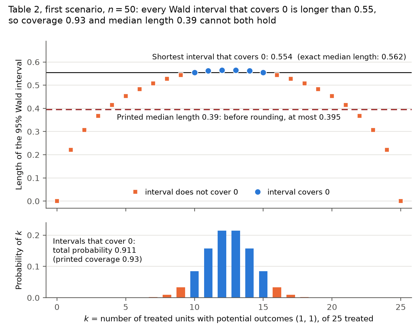
Two stacked panels with a common horizontal axis, k from 0 to 25, the number of treated units with potential outcomes (1,1). Upper panel: the length of the 95 percent Wald interval for each k, rising from 0 at k = 0 to about 0.565 at k = 12 and 13 and falling symmetrically. Six blue circles at k = 10 to 15 mark intervals that cover 0, with lengths between 0.554 and 0.565; orange squares mark the other twenty values. A solid line at 0.554 is labelled 'Shortest interval that covers 0: 0.554 (exact median length: 0.562)'. A dashed red line at 0.395 is labelled 'Printed median length 0.39: before rounding, at most 0.395'. Lower panel: bars for the probability of each k, concentrated on k = 8 to 17; the bars for k = 10 to 15 are blue and the label reads 'Intervals that cover 0: total probability 0.911 (printed coverage 0.93)'.
Wald intervals in the stated 50-unit design of Table 2, first scenario. Upper panel: length of the interval for each value of kk; the intervals that cover 0 (circles) all lie on or above the solid line at 0.554, and the dashed line at 0.395 is an upper bound on any median that rounds to 0.39. Lower panel: probability of each kk; the values of kk whose interval covers 0 have total probability 0.911.

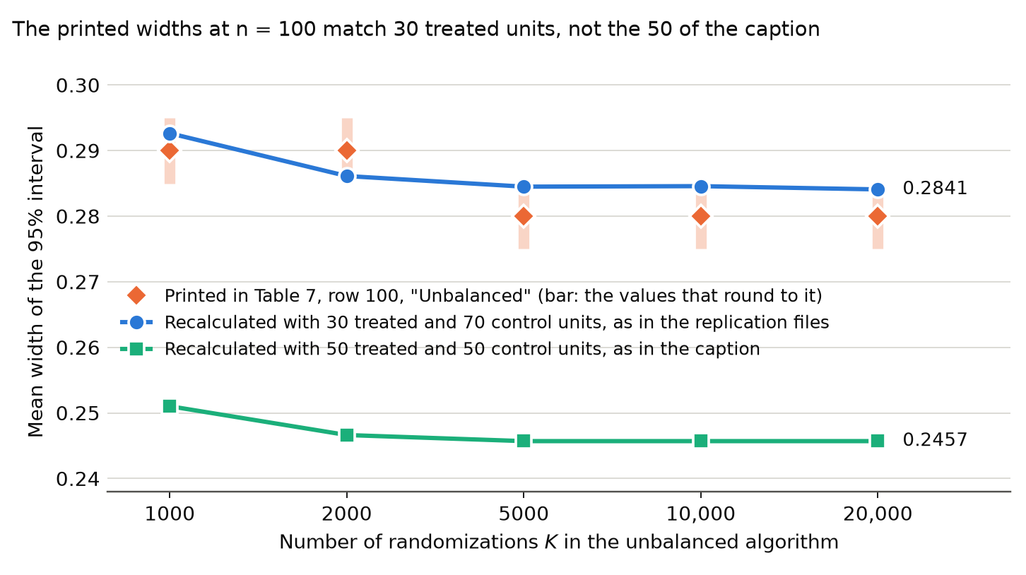
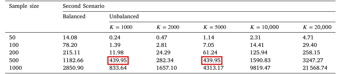
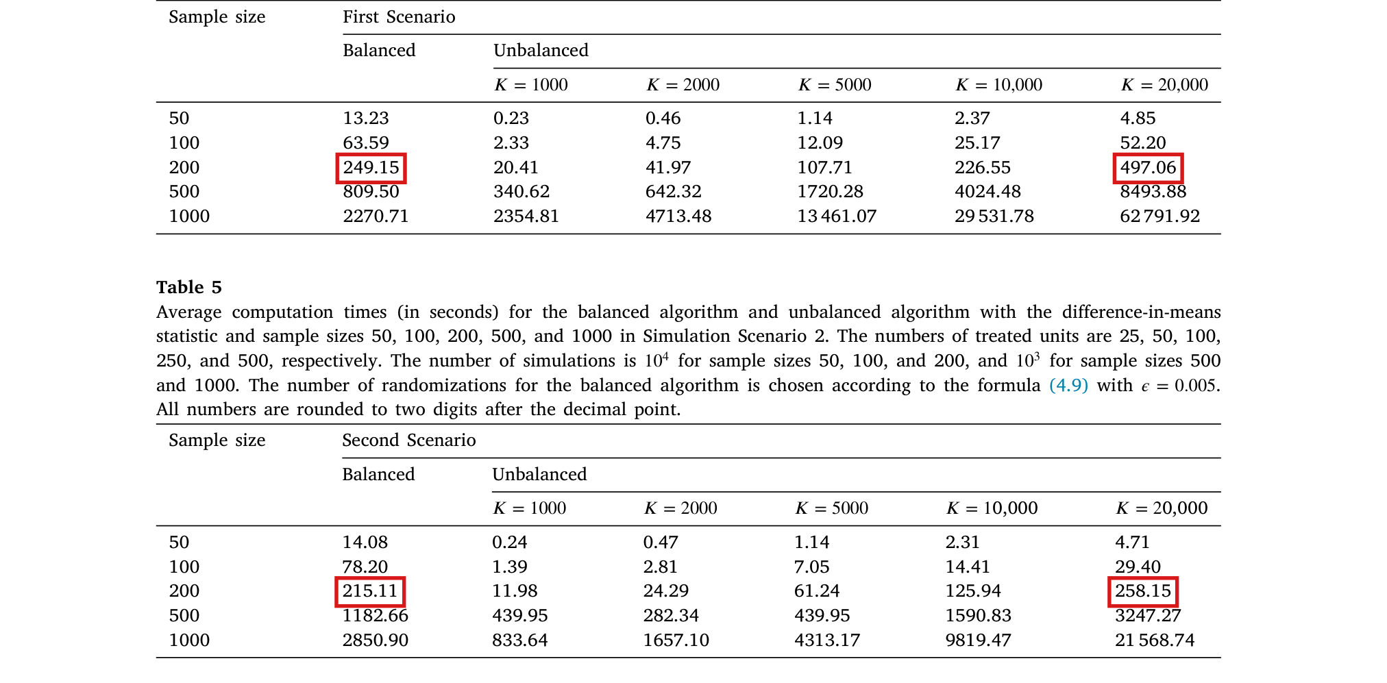
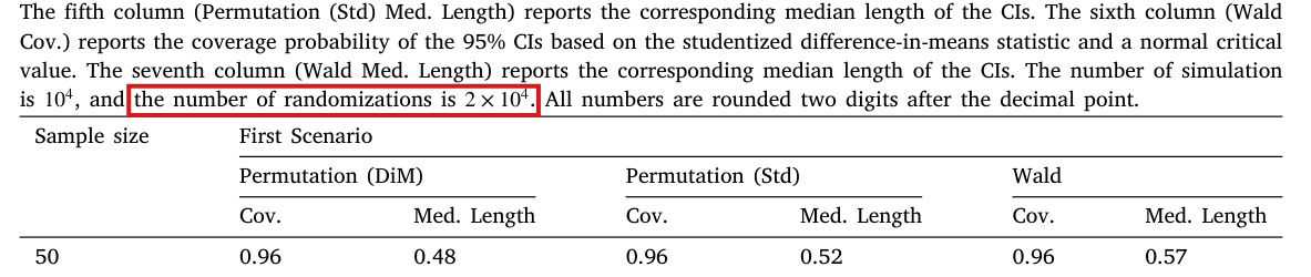
At n=100n = 100 in the second scenario, the simulation script in the replication files runs the unbalanced algorithm with 30 treated units where the captions of Tables 5 and 7 state 50; the widths printed in Table 7 match recalculations with 30 treated units and are incompatible with ordinary 50/50 replication.

Tables 5 and 7, rows for sample size 100, with the sentence on treated units in both captions, pp. 16–17 (PDF pp. 16–17); replication code 1_simulation_unbalanced_case_balanced_design_2.R, lines 24 and 50–53

As printed

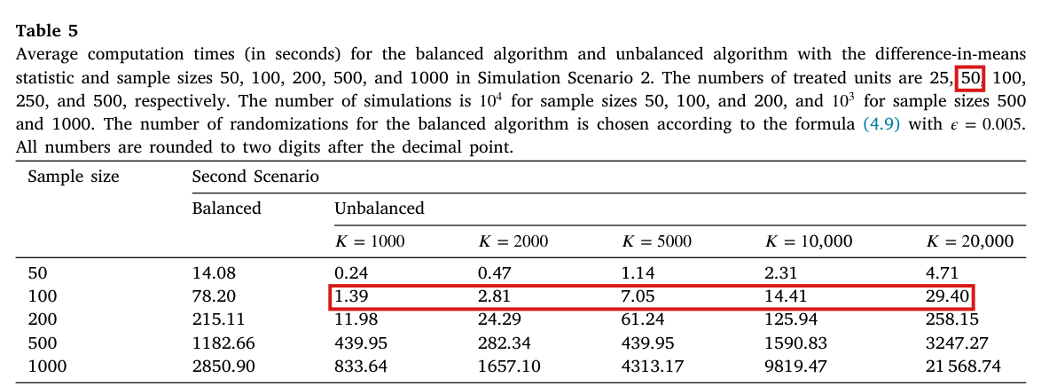
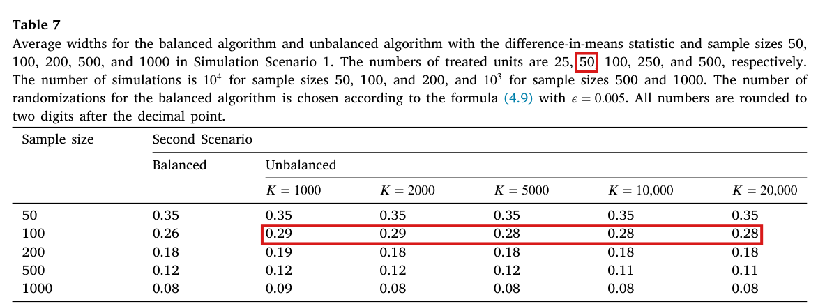
Table 5, caption: “Average computation times (in seconds) for the balanced algorithm and unbalanced algorithm with the difference-in-means statistic and sample sizes 50, 100, 200, 500, and 1000 in Simulation Scenario 2. The numbers of treated units are 25, 50, 100, 250, and 500, respectively.” The caption of Table 7 contains the same sentence on treated units.

Tables 5 and 7, Second Scenario, rows for sample size 100. The first numerical column is the balanced algorithm and the other five are the unbalanced algorithm.
BalancedK=1000K = 1000K=2000K = 2000K=5000K = 5000K=10,000K = 10{,}000K=20,000K = 20{,}000
Table 5 (seconds)78.2078.201.391.392.812.817.057.0514.4114.4129.4029.40
Table 7 (width)0.260.260.290.290.290.290.280.280.280.280.280.28

Replication code (not printed in the article), lines 24, 50 and 51 of the script

1_simulation_unbalanced_case_balanced_design_2.R:

#The number of treated units is nt=0.5*n.

n=100

nt=30

The problem

Tables 5 and 7 describe a comparison of the balanced and the unbalanced algorithm on balanced designs. For n=100n = 100 the captions state 50 treated units, and the script for the balanced algorithm sets 50. The script that runs the unbalanced algorithm in the second scenario sets 30 treated units at n=100n = 100, below a comment that says the number of treated units is n/2n/2. It sets 25 and 100 at n=50n = 50 and n=200n = 200, and the script for the first scenario sets 50 at n=100n = 100. If generated by these scripts, the “Unbalanced” entries at n=100n = 100 come from trials with 30 treated and 70 control units, and the “Balanced” entry comes from trials with 50 and 50.

The widths printed in Table 7 match recalculations with 30 treated units. In the second scenario at n=100n = 100, there are 8 units with potential outcomes (1,1)(1,1) and 92 with (0,0)(0,0). Only nine observed tables are possible, and the mean width can be computed exactly. With exact pp-values and 30 treated units it is about 0.28450.2845, in agreement with the scale of the printed 0.28 to 0.29. With 50 treated units it is 0.26000.2600, and the permutation routine of the replication files returns about 0.250.25; neither value rounds to 0.28. In Table 7 the intervals of the unbalanced algorithm appear wider than those of the balanced one at n=100n = 100 (0.28 to 0.29 against 0.26). I take these recalculations as strong evidence that the allocation mismatch explains this excess width. The table script takes the run times of Table 5 from the same output records as the widths. If the scripts in the replication files produced that row, its five run times belong to the design with 30 treated units as well. The original outputs are not in the replication files, so I cannot establish which script version produced either printed row.

Evidence an exact counterexample

The evidence is a recalculation from the replication files, together with an exact enumeration. A trace of the R functions in the replication files shows that the script generates 30 treated and 70 control observations at n=100n = 100 and passes 30 to the permutation routine for all five values of KK. The script for the balanced algorithm generates 50 and 50. Let n=100n = 100, let the count vector be v=(8,0,0,92)\mathbf{v} = (8, 0, 0, 92), and take the difference-in-means statistic with α=0.05\alpha = 0.05. I enumerate the nine possible observed tables with their hypergeometric probabilities. With exact pp-values, I find that the mean width of the interval is

1350=0.2600for m=50,1764733666962029298100≈0.2845for m=30.\frac{13}{50} = 0.2600 \quad \text{for } m = 50, \qquad \frac{17647336669}{62029298100} \approx 0.2845 \quad \text{for } m = 30 .

For m=50m = 50 the width is 0.260.26 for every observed table. The permutation routine of the replication files was also run at each KK on the nine tables, and the widths were averaged with the same probabilities. The results are in the table below. For each KK, the value for 30 treated units rounds to the printed entry and the value for 50 treated units rounds to 0.25. These values come from one to six runs of the routine per observed table, and they are not replacement entries for Table 7. For m=50m = 50 and K=20,000K = 20{,}000 the expected width is at most 0.2600020.260002, and the probability that the mean over 10410^4 independent simulated experiments rounds to 0.28 or more is below 1.2×10−251.2 \times 10^{-25}. These calculations do not supply replacement run times for Table 5.

Mean width of the interval of the unbalanced algorithm at n=100n = 100 in the second scenario: the entries of Table 7 and Monte Carlo estimates from the permutation routine of the replication files.
KKPrinted in Table 730 treated units50 treated units
100010000.290.290.29260.29260.25100.2510
200020000.290.290.28610.28610.24660.2466
500050000.280.280.28450.28450.24570.2457
10,00010{,}0000.280.280.28460.28460.24570.2457
20,00020{,}0000.280.280.28410.28410.24570.2457
What survives

The repair changes one number in a simulation script and adds no assumption. In both designs the sample average treatment effect is zero, and Algorithm 5.3 is valid for either allocation. The other sample sizes of Tables 5 and 7, the first scenario in Tables 4 and 6, Tables 1–3 and the theoretical results are unaffected by this allocation error. One row does not refute the recommendation of Section 7.2 on the choice of algorithm. The row for n=100n = 100 cannot serve as a comparison on a common design until it is recomputed, and the replacement run times and widths are not known.

Corrected

Replication code, lines 50 and 51 of the script

1_simulation_unbalanced_case_balanced_design_2.R:

n=100

nt=50

The five “Unbalanced” entries of the row for sample size 100 in Table 5 and the five in Table 7 are then to be recomputed for K=1000K = 1000, 20002000, 50005000, 10,00010{,}000 and 20,00020{,}000, with the computing environment of the run times recorded. If the original output files exist, they should be examined before the ten printed entries are attributed to a particular version of the script. The script for a third scenario, which the paper does not report, sets nt=30 at n=100n = 100 in the same way; that is a separate correction.

Crop of Table 5 with its caption. The caption reads: Average computation times (in seconds) for the balanced algorithm and unbalanced algorithm with the difference-in-means statistic and sample sizes 50, 100, 200, 500, and 1000 in Simulation Scenario 2. The numbers of treated units are 25, 50, 100, 250, and 500, respectively. A red outline surrounds the number 50 in this list. The table has the columns Sample size, Balanced, and Unbalanced with K = 1000, 2000, 5000, 10,000 and 20,000. A second red outline surrounds the five Unbalanced entries of the row for sample size 100: 1.39, 2.81, 7.05, 14.41, 29.40. The Balanced entry of that row is 78.20.
Table 5, p. 16. The outlines mark the number of treated units that the caption states for sample size 100 and the five run times of the unbalanced algorithm in that row.
Crop of Table 7 with its caption. The caption reads: Average widths for the balanced algorithm and unbalanced algorithm with the difference-in-means statistic and sample sizes 50, 100, 200, 500, and 1000 in Simulation Scenario 1. The numbers of treated units are 25, 50, 100, 250, and 500, respectively. A red outline surrounds the number 50 in this list. The table is headed Second Scenario and has the columns Sample size, Balanced, and Unbalanced with K = 1000, 2000, 5000, 10,000 and 20,000. A second red outline surrounds the five Unbalanced entries of the row for sample size 100: 0.29, 0.29, 0.28, 0.28, 0.28. The Balanced entry of that row is 0.26. The other rows read 0.35 throughout for sample size 50; 0.18, 0.19, 0.18, 0.18, 0.18, 0.18 for 200; 0.12, 0.12, 0.12, 0.12, 0.11, 0.11 for 500; and 0.08, 0.09, 0.08, 0.08, 0.08, 0.08 for 1000.
Table 7, p. 17. The outlines mark the same number of treated units in the caption and the five widths of the unbalanced algorithm in the row for sample size 100. The width of the balanced algorithm in that row is 0.26.
Line chart. The horizontal axis is the number of randomizations K in the unbalanced algorithm, with the five values 1000, 2000, 5000, 10,000 and 20,000. The vertical axis is the mean width of the 95 percent interval, from 0.24 to 0.30. The title reads: The printed widths at n = 100 match 30 treated units, not the 50 of the caption. Orange diamonds mark the entries printed in Table 7, row 100, Unbalanced: 0.29, 0.29, 0.28, 0.28, 0.28, each with a pale bar from 0.005 below to 0.005 above it. A blue line with circles, labelled recalculated with 30 treated and 70 control units, as in the replication files, runs from 0.2926 at K = 1000 through 0.2861 and 0.2845 to 0.2841 at K = 20,000, and every circle lies inside the bar of the printed entry. A green line with squares, labelled recalculated with 50 treated and 50 control units, as in the caption, runs from 0.2510 at K = 1000 to 0.2457 at K = 20,000, about 0.03 to 0.04 below the printed entries.
Mean width of the interval of the unbalanced algorithm at n=100n = 100 in the second scenario, by number of randomizations KK. The entries printed in Table 7 (orange diamonds; each bar covers the values that round to the entry) agree, after rounding, with Monte Carlo estimates for 30 treated units (blue circles) and lie well above those for 50 treated units (green squares).

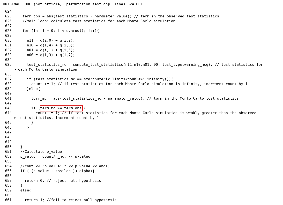
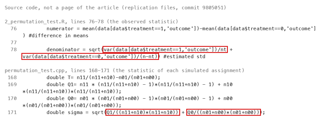
The released code compares the permuted and the observed statistic in double precision and so drops permutations that tie with the observed statistic, which definitions (4.6) and (5.1) count; the comparison should be made on integer counts.

Algorithm 4.4, equation (4.6), p. 9 (PDF p. 9), and equation (5.1), p. 10; released code permutation_test.cpp, function perm_test_inner, lines 625 and 641–645

As printed

Algorithm 4.4, equation (4.6), p. 9.

Vi=1(∣T(n(i))−τ(w~)∣≥∣T(n)−τ(w~)∣),i∈[ ⁣[1,K] ⁣],V_i=\mathbb{1}\Bigl(\bigl|T(\mathbf n^{(i)})-\tau(\widetilde{\mathbf w})\bigr|\ge\bigl|T(\mathbf n)-\tau(\widetilde{\mathbf w})\bigr|\Bigr),\qquad i\in[\![1,K]\!],

Section 1.5, p. 4. Code implementing our proposed algorithms and replicating the tables provided in Section 7 is available at …

Released code, permutation_test.cpp, lines 625, 641 and 643–645 (comments omitted; all three quantities are of type double).

term_obs = abs(test_statistics - parameter_value);

term_mc = abs(test_statistics_mc - parameter_value);

if (term_mc >= term_obs){ count += 1; }

The problem

Definitions (2.12), (4.6) and (5.1) place in the tail every permutation whose centered statistic is at least as large in absolute value as the observed one, ties included. For the difference in means, both sides lie on a lattice, and ties have positive probability. The released function perm_test_inner forms the two sides as double-precision numbers and compares them with >=. Two quantities that are equal as rational numbers can then differ in the last binary digit, and a tie is counted or dropped according to the rounding.

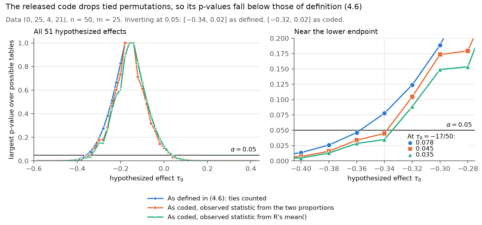
For example, let n=50n=50 and m=25m=25, with observed counts (n11,n10,n01,n00)=(0,25,4,21)(n_{11},n_{10},n_{01},n_{00})=(0,25,4,21) and the possible table v=(4,0,17,29)\mathbf v=(4,0,17,29), for which τ=−17/50\tau=-17/50. For the permuted counts (0,25,13,12)(0,25,13,12), I have ∣T−τ∣=9/50|T-\tau|=9/50, the same value as for the observed counts. In double precision, with the observed statistic computed from the two proportions, the permuted side is smaller by 2−552^{-55}, and the permutation is not counted. Summing over all assignments, I find that the pp-value of this table is 0.07770.0777 as defined. The indicator as coded has expectation 0.03830.0383 when the observed statistic is computed from the two proportions, and 0.02830.0283 when it is computed with the R function mean, as the released wrapper does (R 4.4.2). Since the expectation of the coded indicator differs from the pp-value, more Monte Carlo draws do not remove the difference.

The interval changes as well. Inverting the fully enumerated tails over all 28602860 possible tables at level 0.050.05, I obtain [−17/50,1/50][-17/50,1/50] with the tail as defined and [−8/25,1/50][-8/25,1/50] with the coded comparison. The latter interval is a strict subset, of width 0.340.34 against 0.360.36. Since Proposition 4.6 and Theorem 5.5 concern the procedures with the tail as defined, their coverage guarantees do not carry over to the released code as it stands. The routines for the difference in means, in balanced and in general designs, both call this function. The permutation columns of Tables 2–7 may be affected, but which printed entries change is not established.

Evidence an exact counterexample

The evidence is an exact counterexample. I summed exact integer assignment counts over all possible count states, using rational arithmetic for the probabilities and double precision only for the coded comparison. I also checked the 3715837158 indicators of the examples against the unchanged function perm_test_inner, compiled from the released source.

The table v=(4,0,17,29)\mathbf v=(4,0,17,29) for the data (0,25,4,21)(0,25,4,21), n=50n=50, m=25m=25: numbers of assignments and the corresponding probabilities.
Set of assignmentsNumberProbability
All assignments12641060643775212641060643775211
Tail as defined in (4.6)981667390540298166739054020.07770.0777
Ties with the observed statistic653155084335065315508433500.05170.0517
Tail as coded, observed statistic from the two proportions483819423956748381942395670.03830.0383
Tail as coded, observed statistic from mean in R357115160485235711516048520.02830.0283

Over the 5555 possible tables with τ=−17/50\tau=-17/50, the largest pp-value is 0.07770.0777 as defined, and 0.04470.0447 or 0.03480.0348 as coded. Both coded values are below 0.0450.045, the threshold that the simulation settings apply to the Monte Carlo fraction. In a second example, with the data (8,4,5,7)(8,4,5,7) of the third row of Table 1 and the possible table (10,0,3,11)(10,0,3,11), the pp-value is 57388/676039=0.084957388/676039=0.0849 as defined and 881/29393=0.0300881/29393=0.0300 as coded with the observed statistic from mean in R 4.4.2: the code drops all 148500148500 tied assignments out of 27041562704156.

These checks do not establish undercoverage of an interval. They also do not determine which entries of Tables 2–7 the defect changed: the original simulation outputs are not in the replication files, and I have not repeated the full simulations.

What survives

Definitions (2.12), (4.6) and (5.1), the algorithms as printed and the theorems about them are untouched. The estimand, the construction for missing outcomes and the Wald columns of the tables do not involve this comparison. What changes is the released code, and the permutation columns of Tables 2–7 should be recomputed after the repair.

Corrected

Definition (4.6) stands. In the released code, the tail event for the difference in means is decided on integers. Let uu and ww be the numbers of successes in the treatment group and in the control group, and let d=v10−v01d=v_{10}-v_{01}, so that T=u/m−w/(n−m)T=u/m-w/(n-m) and τ=d/n\tau=d/n. Multiplying ∣T−τ∣|T-\tau| by nm(n−m)nm(n-m) gives the integer

C(u,w;d)=∣n((n−m)u−mw)−d m(n−m)∣,C(u,w;d)=\bigl|n\bigl((n-m)u-mw\bigr)-d\,m(n-m)\bigr|,

and the indicator of (4.6) is computed as

Vi=1(C(u(i),w(i);d)≥C(u,w;d)),V_i=\mathbf 1\bigl(\colorbox{#ffe58a}{$\displaystyle C(u^{(i)},w^{(i)};d)\ge C(u,w;d)$}\bigr),

where (u(i),w(i))(u^{(i)},w^{(i)}) are the success counts of the iith permuted assignment and (u,w)(u,w) are those of the observed data. The integer type must be wide enough to avoid overflow. A fixed floating-point tolerance is not a general guarantee of exactness. The simulation results that use this function must then be recomputed.

Crop of the opening of Algorithm 4.4 on page 9 with equation (4.6), which defines the indicator V i as 1 when the absolute value of T(n(i)) minus tau(w tilde) is greater than or equal to the absolute value of T(n) minus tau(w tilde). A red outline surrounds the greater-than-or-equal sign.
Algorithm 4.4, p. 9 (PDF p. 9). The outline marks the weak inequality in (4.6): a permutation that ties with the observed statistic belongs to the tail.
Listing of lines 624 to 661 of the C++ file permutation_test.cpp, with line numbers. Line 625 sets term_obs to the absolute value of test_statistics minus parameter_value. Line 641 sets term_mc in the same way from the simulated statistic. Line 643 reads: if (term_mc >= term_obs), followed by count += 1. A red outline surrounds the comparison term_mc >= term_obs.
Function perm_test_inner of permutation_test.cpp, lines 624–661 (a listing of the released code, not a page of the article). The outline marks the comparison on line 643; its two sides are the double-precision quantities set on lines 625 and 641.
Two line charts of the largest p-value against the hypothesized effect, titled: The released code drops tied permutations, so its p-values fall below those of definition (4.6). The left chart covers all 51 effects from -0.58 to 0.42: three curves rise from 0 to 1 near -0.16 and fall back to 0, and the two curves labelled as coded lie on or below the curve labelled as defined. The right chart shows effects from -0.40 to -0.28 with a horizontal line at alpha = 0.05. At -0.34 the curve as defined is at 0.078, above the line, and the two curves as coded are at 0.045 and 0.035, below the line. A subtitle states that inverting at 0.05 gives the interval from -0.34 to 0.02 as defined and from -0.32 to 0.02 as coded.
The largest pp-value over the possible tables, for each hypothesized effect τ0\tau_0, for the data (0,25,4,21)(0,25,4,21) with n=50n=50 and m=25m=25: with the tail as defined in (4.6) (circles), and with the comparison of the released code in double precision, for the observed statistic computed from the two proportions (squares) and with mean in R (triangles). At τ0=−17/50\tau_0=-17/50 the values are 0.0780.078, 0.0450.045 and 0.0350.035, so this effect is accepted at level 0.050.05 under the definition and rejected by the coded comparison.

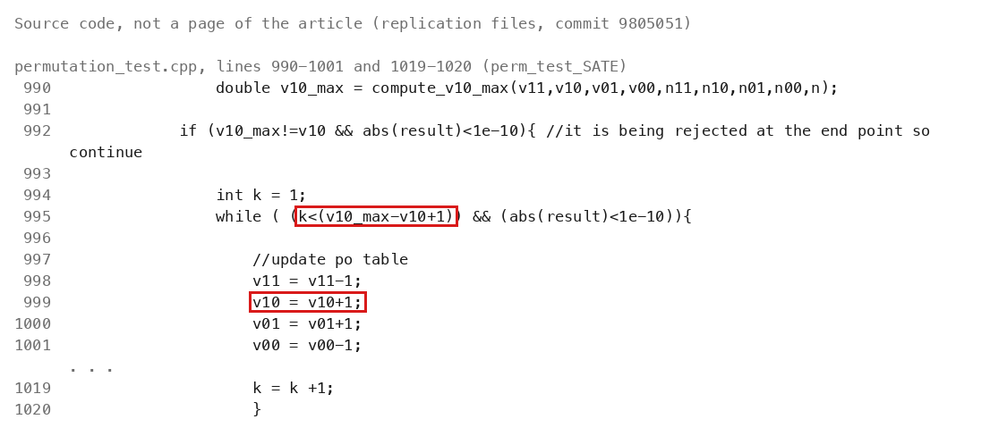
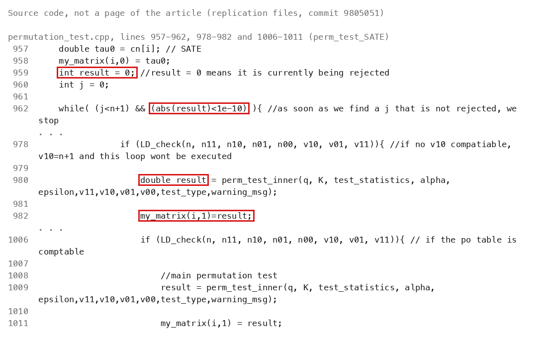
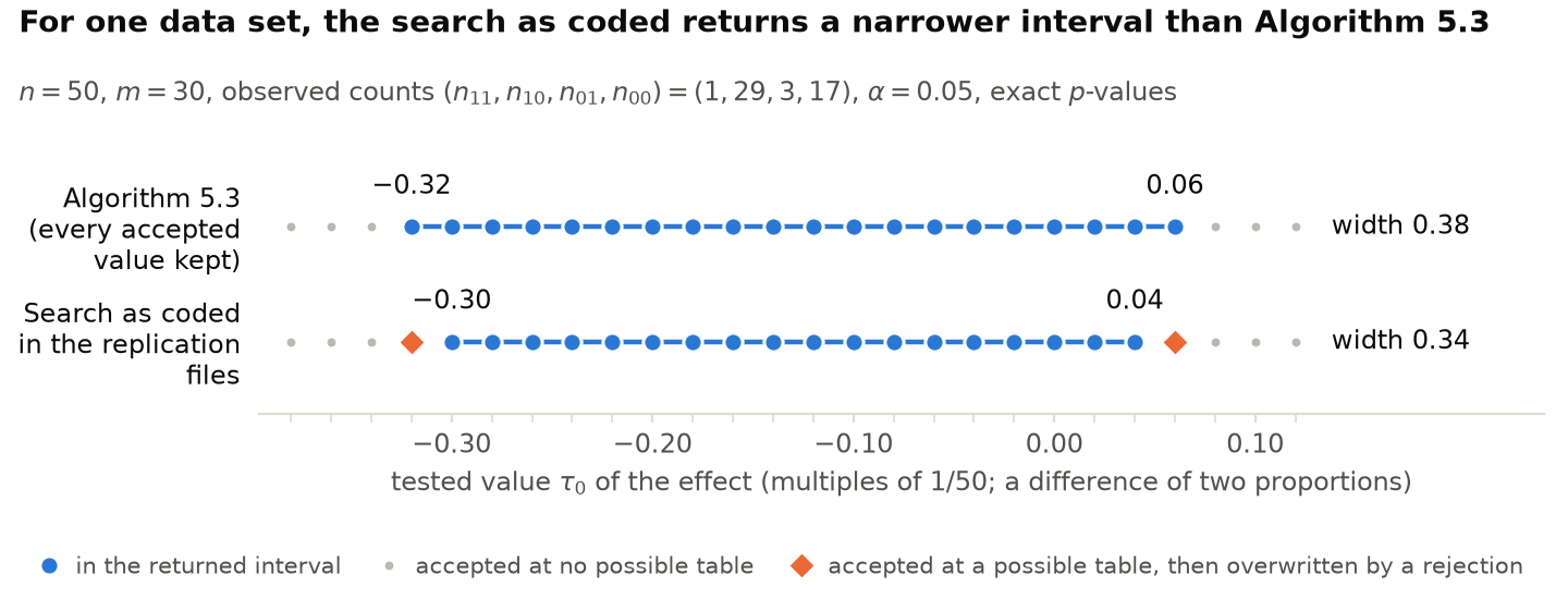
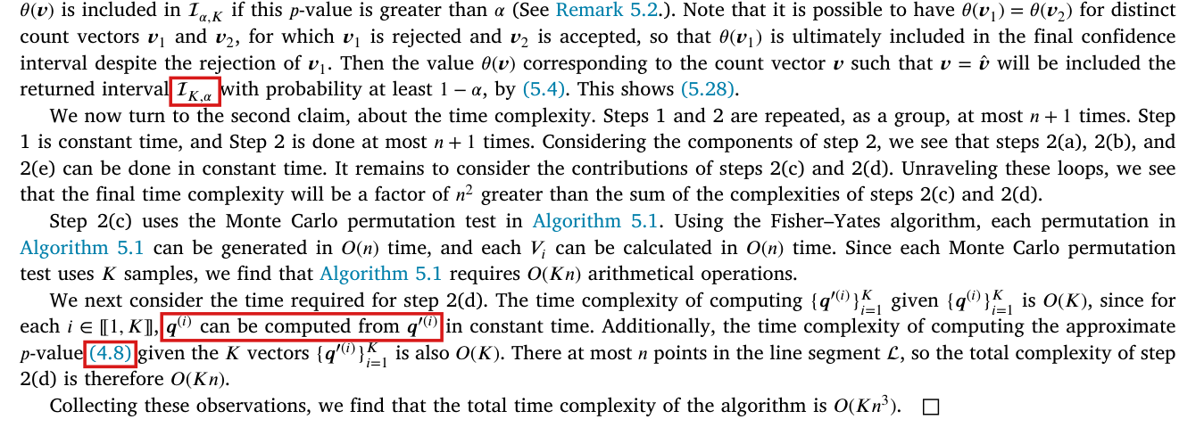
Five loops in the released code compute their bound from the count that they advance, allowing at most about half the steps along each line of count vectors; the code can stop before completing the search described in Section 5.1.1.

Section 5.1.1, p. 13 (PDF p. 13), paragraph before (5.27); replication files, permutation_test.cpp, lines 475, 803, 906, 995 and 1204; Table 3 and Tables 4–7, pp. 16–17

As printed

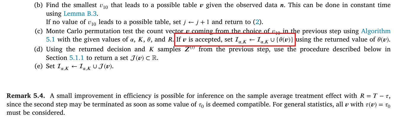
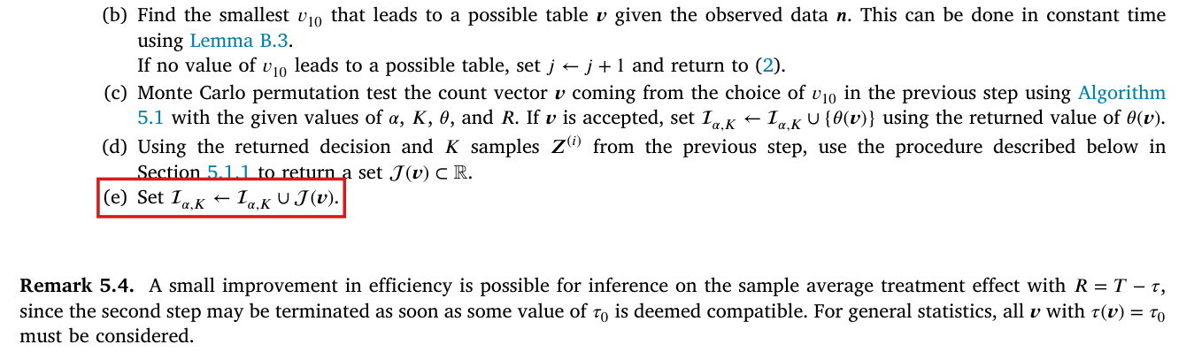
P. 13: “Iterating this procedure allows us to search the entire line segment L\mathcal L to find the set V\mathcal V consisting of vk∈L\boldsymbol v_k\in\mathcal L that are both possible and would be accepted by an application of Algorithm 5.1 (where possibility is checked using Lemma B.3).”

Replication files, permutation_test.cpp, routine perm_test_SATE, lines 995, 998–1001 and 1019:

while ( (k<(v10_max-v10+1)) && (abs(result)<1e-10)){

v11 = v11-1;

v10 = v10+1;

v01 = v01+1;

v00 = v00-1;

k = k +1;

Line 1204 has the same condition. Lines 475, 803 and 906 read for (int k=1; k<(v10_max-v10+1); k++){, with the same four updates in the body.

The problem

Section 5.1.1 tests every possible additional vector vk\mathbf v_k on L\mathcal L, starting from the vector v\mathbf v already tested in Step 2(c), updating the Monte Carlo draws from one vector to the next. The proof of Theorem 5.5 in Appendix C relies on the true count vector being among the vectors tested. In the code, each of the five loops runs while kk is less than v10_max-v10+1, and the body of the loop increases v10 by one. The bound falls by one at every step while kk rises by one. Let dd be the difference between v10_max and v10 on entering the loop, which is the number of steps needed to reach the end of the line. Without an earlier stop at acceptance, the loop makes only ⌈d/2⌉\lceil d/2\rceil of them. The bound alone omits the last ⌊d/2⌋\lfloor d/2\rfloor vectors, and for d≥2d\ge 2 the end of the line is not reached. The bound does not involve KK, and more Monte Carlo draws do not restore the omitted tests. The same bound appears in the routine that sizes the output (line 475), in the two routines for general estimands that serve the risk ratio and the odds ratio (lines 803 and 906), and in the two routines for the sample average treatment effect (lines 995 and 1204). The supplied replication workflows call the last two for the permutation columns of Table 3, and perm_test_SATE for the “Unbalanced” columns of Tables 4–7. The full-search coverage argument therefore does not by itself establish coverage for this code, and the affected interval and timing comparisons need checking with corrected code.

Evidence an exact counterexample

The evidence is a derivation and an exact counterexample, confirmed by compiling the original routines. Let aa be the value of v10 on entering the loop and bb the value of v10_max, so that d=b−ad=b-a. After k−1k-1 steps, v10 equals a+k−1a+k-1, and the length condition for step kk is

k<b−(a+k−1)+1=d−k+2.k<b-(a+k-1)+1=d-k+2 .

For integers this is equivalent to 2k≤d+12k\le d+1, and hence to k≤⌈d/2⌉k\le\lceil d/2\rceil.

For the counterexample, take the observed counts (1,1,1,1)(1,1,1,1), τ0=0\tau_0=0 and j=2j=2. The line is (2,0,0,2)(2,0,0,2), (1,1,1,1)(1,1,1,1), (0,2,2,0)(0,2,2,0), and v10_max is 2.

The loop as coded on the line τ0=0\tau_0=0, j=2j=2 for the observed counts (1,1,1,1)(1,1,1,1).
step kkv10 before the stepbound v10_max-v10+1k<k<{}boundvector reached
103true(1,1,1,1)(1,1,1,1)
212falsenone: (0,2,2,0)(0,2,2,0) is not tested

Of the 15 count vectors that are possible given these data, the code visits 14. When compiled, the sizing routine returns 14 and the set routine returns 14 rows; both counts become 15 once the five bounds are replaced. The omitted vector (0,2,2,0)(0,2,2,0) can be the count vector of the true table: with two subjects of type (1,0)(1,0) and two of type (0,1)(0,1), the observed counts (1,1,1,1)(1,1,1,1) have probability 2/32/3. Its risk ratio is 1 and its exact pp-value is 1 for the risk-ratio test.

For the data set with n=50n=50, m=30m=30 and observed counts (1,29,3,17)(1,29,3,17), I find the following counts.

Count vectors with a given τ0\tau_0 for the observed counts (1,29,3,17)(1,29,3,17): those possible, and those reached by the loop as coded before any stop at an acceptance.
nτ0n\tau_0possible count vectorsreached by the loop as coded
337346
−16-167849
227849
−15-158352

Note that an omitted vector need not remove its value of the estimand. In the four-unit example the tested vector (2,0,0,2)(2,0,0,2) also has risk ratio 1 and pp-value 1. For the four values of τ0\tau_0 in the second table, the largest exact pp-value of the difference-in-means test is the same over the full and the truncated sets of vectors. I have not established a changed interval, coverage or printed number; the original simulation outputs are unavailable.

What survives

This code defect does not contradict the full-search procedure of Section 5.1.1, Algorithm 5.3, Theorem 5.5 or the O(Kn3)O(Kn^3) bound. The routines for the difference in means in balanced designs contain none of the five loops. Table 2, the “Balanced” columns of Tables 4–7 and the Wald columns are unaffected by these bounds. The supplied code for the permutation columns of Table 3 and the “Unbalanced” columns of Tables 4–7 makes fewer tests than Algorithm 5.3 requires whenever a line with d≥2d\ge 2 must be searched to its end: a full search takes dd steps where the code takes ⌈d/2⌉\lceil d/2\rceil. The interval and timing comparisons must be checked again with corrected code.

Corrected

In all five loops, compare the count with its fixed maximum. Lines 995 and 1204 become

while ( (v10<v10_max) && (abs(result)<1e-10)){

and lines 475, 803 and 906 become

for (int k=1; v10<v10_max; k++){

An equivalent change is to store dd, the difference between v10_max and v10, before the loop and to iterate over k=1,…,dk=1,\ldots,d. The sizing routine must be changed together with the enumeration, and the two routines for the sample average treatment effect keep their stop at an acceptance. The sentence of Section 5.1.1 needs no change.

Crop of the paragraph that ends with equation (5.27), J = {theta(v) : v in V}. Red boxes mark the words 'Iterating this procedure allows us to search the entire line' at the end of one line and 'segment L' at the start of the next. The sentence continues 'to find the set V consisting of v_k in L that are both possible and would be accepted by an application of Algorithm 5.1 (where possibility is checked using Lemma B.3).'
Section 5.1.1, p. 13 (PDF p. 13), the paragraph before (5.27). The marked sentence says that the whole line segment L\mathcal L is searched. This is the intended search; the released code’s shrinking bound can stop it early.
Listing of source code with line numbers. Line 990 computes v10_max. A red box marks the condition 'k<(v10_max-v10+1)' in line 995, a while loop with the two conditions (k<(v10_max-v10+1)) and (abs(result)<1e-10). A second red box marks line 999, 'v10 = v10+1;', among the four updates v11 = v11-1; v10 = v10+1; v01 = v01+1; v00 = v00-1; of lines 998 to 1001. Line 1019 is 'k = k +1;'.
Source code of the replication files, not a page of the article: permutation_test.cpp, lines 990–1001 and 1019–1020 (routine perm_test_SATE). The marked bound of line 995 contains v10, which the marked line 999 increases at every step, so the bound falls by one each time kk rises by one.

In the released routines for the sample average treatment effect, a variable declared inside a block hides the flag that should hold an acceptance; a later rejection can then erase an accepted table, and the code can exclude values that Algorithm 5.3 keeps.

Algorithm 5.3, Step 2(c), and Remark 5.4, p. 12 (PDF p. 12); replication files, permutation_test.cpp, lines 959–982 and 1167–1190; Table 3 and Tables 4–7, pp. 16–17

As printed

P. 12, Algorithm 5.3, Step 2(c): “Monte Carlo permutation test the count vector v\mathbf v coming from the choice of v10v_{10} in the previous step using Algorithm 5.1 with the given values of α\alpha, KK, θ\theta, and RR. If v\mathbf v is accepted, set Iα,K←Iα,K∪{θ(v)}\mathcal I_{\alpha,K}\leftarrow\mathcal I_{\alpha,K}\cup\{\theta(\mathbf v)\} using the returned value of θ(v)\theta(\mathbf v).”

Replication files, permutation_test.cpp, routine perm_test_SATE, lines 959, 962, 980 and 982:

int result = 0; //result = 0 means it is currently being rejected

while( (j<n+1) && (abs(result)<1e-10) ){ //as soon as we find a j that is not rejected, we stop

double result = perm_test_inner(q, K, test_statistics, alpha, epsilon,v11,v10,v01,v00,test_type,warning_msg);

my_matrix(i,1)=result;

Routine perm_test_SATE_STD, line 1188:

double result = perm_test_inner_STD(q, K, test_statistics_num, test_statistics_den, alpha, epsilon,v11,v10,v01,v00,test_type,warning_msg);

The problem

Algorithm 5.3 adds θ(v)\theta(\mathbf v) to the confidence set whenever a possible table v\mathbf v is accepted, and no later step removes it. Remark 5.4 allows the search over the tables with a given τ0\tau_0 to stop at the first acceptance. The routines perm_test_SATE and perm_test_SATE_STD implement this search with an integer flag result, set to 0 before the loop, and a loop that runs while the flag is 0. At the first table of each line of tables, the outcome of the test is assigned to a new variable, also named result, that exists only inside the enclosing block (line 980, and line 1188 in the studentized routine). After an acceptance the flag is still 0. The search continues, and each later test overwrites the stored decision. A value τ0\tau_0 that has an accepted possible table can therefore be returned as rejected if a later rejection overwrites the acceptance and no subsequent acceptance survives. For given decisions of the individual tests, the set returned by the code is contained in the set of Algorithm 5.3, and it can be strictly smaller. The replication files use these routines for the “Permutation (DiM)” and “Permutation (Std)” columns of Table 3, and the first of them for the “Unbalanced” columns of Tables 4–7. Theorem 5.5 describes a procedure in which an accepted value is never removed. Its coverage statement does not transfer to these routines as released.

Evidence an exact counterexample

The evidence is a set of exact counterexamples. I computed the pp-values in rational arithmetic and checked the compiled routines using all assignments in the small examples, with and without the two declarations.

First, let n=3n=3, m=1m=1, α=1/2\alpha=1/2, ε=0\varepsilon=0 and τ0=1/3\tau_0=1/3, with observed counts (0,1,0,2)(0,1,0,2). Exactly two possible tables have this τ0\tau_0, and neither line contains a further table.

The search as coded for τ0=1/3\tau_0=1/3. The value 1/31/3 is accepted at j=1j=1 and returned as rejected.
jjtable v\mathbf vexact pp-valuetest at α=1/2\alpha=1/2stored decisionflag after the test
1(0,1,0,2)(0,1,0,2)11accept10
2(0,2,1,0)(0,2,1,0)1/31/3reject00

With double removed, the search stops at j=1j=1 and returns acceptance, as Algorithm 5.3 does. For the population with one subject of type (1,0)(1,0) and two of type (0,0)(0,0), whose effect is 1/31/3, the interval of the search as coded covers the effect with probability 1/31/3 at nominal level 1/21/2 when the tests are exact, and with probability below 0.3340.334 when K=300K=300.

Second, let n=50n=50, m=30m=30, α=0.05\alpha=0.05 and ε=0\varepsilon=0, with observed counts (1,29,3,17)(1,29,3,17), using exact pp-values in place of Monte Carlo ones. At τ0=3/50\tau_0=3/50 the ten accepted possible tables v=(4,j−4,j−7,57−2j)\mathbf v=(4,j-4,j-7,57-2j), j=10,…,19j=10,\ldots,19, have exact pp-values between 1962369/38116060≈0.05151962369/38116060\approx 0.0515 and 6295858813/102454809226≈0.06156295858813/102454809226\approx 0.0615, and the search as coded returns rejection. The same happens at τ0=−16/50\tau_0=-16/50. The search as coded returns [−15/50,2/50][-15/50,2/50], of width 0.340.34. Algorithm 5.3 returns [−16/50,3/50][-16/50,3/50], of width 0.380.38, and so does the code with only the two declarations changed. This data set has probability 342/2303342/2303 in the paper’s second scenario with n=50n=50 (four subjects of type (1,1)(1,1) and 46 of type (0,0)(0,0)).

Third, for the studentized routine with ε=0\varepsilon=0 and α=0.05\alpha=0.05, take nine subjects whose potential outcomes are all zero, and m=5m=5. The returned interval covers the effect 00 with probability at most 50/63≈0.79450/63\approx 0.794 for every positive KK divisible by 20. Note that this bound also depends on how the code treats a zero variance. It is not an effect of the hidden flag alone.

No entry of Tables 3–7 has been recomputed. The replication files contain no simulation outputs.

What survives

The set-union instruction in Algorithm 5.3 and the stopping rule in Remark 5.4 need no change; this defect does not refute Theorem 5.5. The balanced routines, Tables 1 and 2, the “Balanced” columns of Tables 4–7, the routines for general estimands, the Wald comparisons and the missing-data construction are not affected by the two declarations. What changes is the standing of the two permutation columns of Table 3 and of the “Unbalanced” columns of Tables 4–7: their intervals can be narrower than those of the method, and their widths and run times must be regenerated with corrected code. Which entries change, and by how much, is not established.

Corrected

In perm_test_SATE (line 980) and perm_test_SATE_STD (line 1188), assign the decision to the flag that already exists:

double result = perm_test_inner(q, K, test_statistics, alpha, epsilon,v11,v10,v01,v00,test_type,warning_msg);

double result = perm_test_inner_STD(q, K, test_statistics_num, test_statistics_den, alpha, epsilon,v11,v10,v01,v00,test_type,warning_msg);

An accepted first table then stops the search for that τ0\tau_0, as Remark 5.4 allows, and cannot be overwritten. The outputs behind Table 3 and the “Unbalanced” columns of Tables 4–7 should be regenerated after this and the other corrections to the code, among them P003-E022 and P003-E024. Algorithm 5.3 needs no change.

Crop of steps (b) to (e) of Algorithm 5.3 and of Remark 5.4. A red box marks, in step (c), the instruction 'If v is accepted, set I_{alpha,K} <- I_{alpha,K} union {theta(v)}'. Remark 5.4 below says that for the sample average treatment effect the second step may be terminated as soon as some value of tau_0 is deemed compatible.
Algorithm 5.3, Steps 2(b)–2(e), and Remark 5.4, p. 12 (PDF p. 12). The marked instruction adds θ(v)\theta(\mathbf v) to the confidence set whenever v\mathbf v is accepted, and nothing later removes it. The passage is correct; the released code departs from it.
Listing of source code with line numbers. Red boxes mark 'int result = 0;' in line 959, the condition '(abs(result)<1e-10)' of the while loop in line 962, the words 'double result' at the start of line 980, and line 982, 'my_matrix(i,1)=result;'. Lines 1006 to 1011 show the later test, 'result = perm_test_inner(...)' without a declaration, followed by 'my_matrix(i,1) = result;'.
Source code of the replication files, not a page of the article: permutation_test.cpp, lines 957–962, 978–982 and 1006–1011 (routine perm_test_SATE). The loop of line 962 runs while the flag of line 959 is zero. Line 980 declares a second variable of the same name, so the flag stays at zero and line 982 stores a decision that later tests overwrite; line 1009 assigns to the flag itself.
Chart with two rows of dots over a horizontal axis of tested values tau_0 from minus 0.38 to 0.12 in steps of 0.02. Top row, Algorithm 5.3 with every accepted value kept: blue dots from minus 0.32 to 0.06, labelled width 0.38. Bottom row, the search as coded in the replication files: blue dots from minus 0.30 to 0.04, labelled width 0.34, and orange diamonds at minus 0.32 and at 0.06, which the legend describes as accepted at a possible table, then overwritten by a rejection. Small grey dots at the other values mark values accepted at no possible table.
The interval for one data set (n=50n=50, m=30m=30, observed counts (1,29,3,17)(1,29,3,17), α=0.05\alpha=0.05), with exact pp-values in place of Monte Carlo ones. Algorithm 5.3 returns [−0.32,0.06][-0.32,0.06]. The search as coded returns [−0.30,0.04][-0.30,0.04]: the values −0.32-0.32 and 0.060.06 are accepted at a possible table, and a later rejection overwrites the acceptance. The data set has probability 342/2303342/2303 in the paper’s second scenario with n=50n=50.

Minor (30)

Real but inconsequential, for example a misprint that does not change a result.

After Step 2(e) of Algorithm 5.3, jj must be increased by one and the algorithm must return to Step 2.

Algorithm 5.3, pp. 11–12 (PDF pp. 11–12), after Step 2(e)

See also under Formal statements (Lean): P003-T22, P003-T35

As printed

P. 11: “For every τ0∈C(n)\tau_0\in\mathcal C(\mathbf n), in descending order from max⁡(C(n))\max(\mathcal C(\mathbf n)), we perform the following steps. 1. Initialize j←0j\leftarrow 0. 2. If j≤nj\le n, perform the following steps.”

P. 12, Step 2(b): “If no value of v10v_{10} leads to a possible table, set j←j+1j\leftarrow j+1 and return to (2).”

P. 12, last step: “(e) Set Iα,K←Iα,K∪J(v)\mathcal I_{\alpha,K}\leftarrow\mathcal I_{\alpha,K}\cup\mathcal J(\mathbf v).” The algorithm ends with this step.

The problem

The loop over j∈[[0,n]]j\in[[0,n]] is advanced only in Step 2(b), in the case where no table is possible. After a possible table has been processed in Steps 2(c)–2(e), nothing increases jj or returns to Step 2. Read literally, the algorithm treats only the first jj with a possible table for each τ0\tau_0. Remark 5.4, the running-time count in Appendix C and the released code all assume the loop over every jj.

Evidence an exact counterexample

The evidence is a check of pp. 11–12 and a small exact example of the literal reading. Let n=2n=2 and m=1m=1, with observed counts (0,1,0,1)(0,1,0,1), the estimand θ(v)=v10+v01\theta(\mathbf v)=v_{10}+v_{01} and the constant statistic R=0R=0, so that every test accepts. If the search stops at the first jj with a possible table, I obtain the tables (0,0,1,1)(0,0,1,1), (0,0,0,2)(0,0,0,2) and (0,1,0,1)(0,1,0,1), and the set {0,1}\{0,1\}. The full loop also reaches (0,1,1,0)(0,1,1,0) and returns {0,1,2}\{0,1,2\}. The table with one subject of type (0,1)(0,1) and one of type (1,0)(1,0) produces these data and has θ=2\theta=2. The released code loops over every jj (for (int j=0; j<n+1; j++)).

What survives

The algorithm as intended, its coverage (Theorem 5.5) and its O(Kn3)O(Kn^3) running time are unaffected once the instruction is restored. The released code already performs the loop over jj.

Corrected

“(e) Set Iα,K←Iα,K∪J(v)\mathcal I_{\alpha,K}\leftarrow\mathcal I_{\alpha,K}\cup\mathcal J(\mathbf v). Set j←j+1\colorbox{#ffe58a}{$j\leftarrow j+1$} and return to (2).”

When j>nj>n, the steps are repeated for the next τ0∈C(n)\tau_0\in\mathcal C(\mathbf n). After the last τ0\tau_0, the algorithm returns Iα,K\mathcal I_{\alpha,K}.

Crop of steps (b) to (e) of Algorithm 5.3 and of Remark 5.4. A red box marks step (e), 'Set I_{alpha,K} <- I_{alpha,K} union J(v).', after which a blank space precedes Remark 5.4. Step (b) above contains the sentence 'If no value of v10 leads to a possible table, set j <- j + 1 and return to (2).'
Algorithm 5.3, Steps 2(b)–2(e), and Remark 5.4, p. 12 (PDF p. 12). The marked step is the last instruction of the algorithm. Only the branch of Step 2(b) in which no table is possible increases jj and returns to Step 2.

The sample average treatment effect in (5.6) is (v10−v01)/n(v_{10}-v_{01})/n: both numerators should read v10−v01v_{10}-v_{01}.

Equation (5.6), p. 11 (PDF p. 11), both numerators

See also under Formal statements (Lean): P003-T13

As printed

“To target the sample average treatment effect, we have already seen that we may use the estimand

θ(v)=τ(v)=v11−v01n=v11−v01v11+v10+v01+v00.(5.6)”\theta(\mathbf v)=\tau(\mathbf v)=\frac{\colorbox{#ffe58a}{$\displaystyle v_{11}$}-v_{01}}{n}=\frac{\colorbox{#ffe58a}{$\displaystyle v_{11}$}-v_{01}}{v_{11}+v_{10}+v_{01}+v_{00}}.\qquad\text{(5.6)''}
The problem

Equation (5.6) restates the sample average treatment effect as the estimand for Algorithm 5.1. By (2.2), vabv_{ab} is the number of subjects whose outcomes under treatment and control are (a,b)(a,b). Then the effect (2.6) is the number of subjects with outcomes (1,0)(1,0) minus the number with outcomes (0,1)(0,1), divided by nn. The display has v11v_{11}, the number of subjects with outcome 1 under both conditions, where v10v_{10} is required. The printed quantity differs from τ(v)\tau(\mathbf v) by (v11−v10)/n(v_{11}-v_{10})/n, and the two agree only when v11=v10v_{11}=v_{10}.

Evidence an exact counterexample

The evidence is a derivation and an exact counterexample. By (2.2), I have ∑jwj(1)=v11+v10\sum_j w_j(1)=v_{11}+v_{10} and ∑jwj(0)=v11+v01\sum_j w_j(0)=v_{11}+v_{01}. Substituting these sums into (2.6), I obtain

τ(w)=(v11+v10)−(v11+v01)n=v10−v01n,\tau(\mathbf w)=\frac{(v_{11}+v_{10})-(v_{11}+v_{01})}{n}=\frac{v_{10}-v_{01}}{n},

and n=v11+v10+v01+v00n=v_{11}+v_{10}+v_{01}+v_{00}. For the counterexample, let n=20n=20 and v=(10,0,0,10)\mathbf v=(10,0,0,10). Every subject has the same outcome under treatment and control. Then τ=0\tau=0, while both printed fractions equal 1/21/2. For v=(0,20,0,0)\mathbf v=(0,20,0,0) I have τ=1\tau=1, and both printed fractions equal 00.

What survives

The definitions (2.2) and (2.6), the constraint (4.2), the construction (5.16) and the calculation (A.7) use the correct expression and are unaffected. The released code computes (v10−v01)/(v11+v10+v01+v00)(v_{10}-v_{01})/(v_{11}+v_{10}+v_{01}+v_{00}), so the misprint does not enter the simulations. Theorem 5.5 is stated for a general estimand θ\theta and does not depend on (5.6).

Corrected

“To target the sample average treatment effect, we have already seen that we may use the estimand

θ(v)=τ(v)=v10−v01n=v10−v01v11+v10+v01+v00,(5.6)”\theta(\mathbf v)=\tau(\mathbf v)=\frac{\colorbox{#ffe58a}{$\displaystyle v_{10}$}-v_{01}}{n}=\frac{\colorbox{#ffe58a}{$\displaystyle v_{10}$}-v_{01}}{v_{11}+v_{10}+v_{01}+v_{00}},\qquad\text{(5.6)''}

where v=(v11,v10,v01,v00)\mathbf v=(v_{11},v_{10},v_{01},v_{00}) is the count vector (2.2) of a potential outcome table of n=v11+v10+v01+v00n=v_{11}+v_{10}+v_{01}+v_{00} subjects.

Crop of the bullet 'To target the sample average treatment effect, we have already seen that we may use the estimand' and of equation (5.6), theta(v) = tau(v) = (v11 - v01)/n = (v11 - v01)/(v11 + v10 + v01 + v00). Red boxes mark v11 in each of the two numerators.
Equation (5.6), p. 11 (PDF p. 11). The two marked terms are the count v11v_{11} of subjects whose outcome is 1 under both treatment and control; the sample average treatment effect has v10v_{10} in both places.

In Definition A.1, display (A.3) needs the restriction 0≤x<y0 \le x < y, and the rescaled function on Z\mathbb{Z} is g(x)=f(x/k)g(x) = f(x/k), not g(x)=f(kx)g(x) = f(kx).

Appendix A, Definition A.1, display (A.3), and the paragraph after the definition, p. 18 (PDF p. 18)

See also under Formal statements (Lean): P003-T9, P003-T10, P003-T14, P003-T15

As printed

If ff is symmetric about k0k_0, we say that ff is decreasing away from k0k_0 if

f(k0+y)≤f(k0+x) for all x,y∈2−1Z such that y>x and k0+x,k0+y∈Z.(A.3)f(k_0 + y) \le f(k_0 + x) \text{ for all } x, y \in 2^{-1}\mathbb{Z} \text{ such that } \colorbox{#ffe58a}{$\displaystyle y > x$} \text{ and } k_0 + x, k_0 + y \in \mathbb{Z}. \qquad \text{(A.3)}

[…] Given k∈Z>0k \in \mathbb{Z}_{>0} and k0∈2−1Zk_0 \in 2^{-1}\mathbb{Z}, we say that a probability mass function f:k−1Z→R≥0f : k^{-1}\mathbb{Z} \to \mathbb{R}_{\ge 0} is symmetric about k−1k0∈(2k)−1Zk^{-1}k_0 \in (2k)^{-1}\mathbb{Z} if the function g:Z→R≥0g : \mathbb{Z} \to \mathbb{R}_{\ge 0} defined by g(x)=f(kx)g(x) = \colorbox{#ffe58a}{$f(kx)$} is symmetric about k0k_0. Similarly, we say that ff is SD if g(x)=f(kx)g(x) = \colorbox{#ffe58a}{$f(kx)$} is.

The problem

As printed, (A.3) requires f(k0+y)≤f(k0+x)f(k_0 + y) \le f(k_0 + x) for every pair x<yx < y, including negative xx. It then asks ff to be non-increasing on all of Z\mathbb{Z}, and no probability mass function has this property. For the point mass at 00, with k0=0k_0 = 0, x=−1x = -1 and y=0y = 0, the condition reads 1≤01 \le 0. The intended condition is that ff decreases with the distance from k0k_0, that is, 0≤x<y0 \le x < y. In the paragraph after the definition, a probability mass function ff on the lattice k−1Zk^{-1}\mathbb{Z} is carried to Z\mathbb{Z} by g(x)=f(kx)g(x) = f(kx). The map that does this is g(x)=f(x/k)g(x) = f(x/k), the probability mass function of kXkX when XX has probability mass function ff. As printed, gg takes the values of ff only at integer multiples of kk. Every later use follows the intended definitions.

Evidence a derivation

The evidence is a derivation with two exact counterexamples. Suppose that ff satisfies (A.3) as printed. For integers a<ba < b, taking x=a−k0x = a - k_0 and y=b−k0y = b - k_0, I have f(b)≤f(a)f(b) \le f(a). If f(b)>0f(b) > 0 for some bb, then f(a)≥f(b)>0f(a) \ge f(b) > 0 for the infinitely many integers a<ba < b, and ff is not summable. This implies that no probability mass function satisfies the printed condition; the point mass at 00 in the paragraph above is one instance. With 0≤x<y0 \le x < y, the condition says that f(k0+x)f(k_0 + x) is non-increasing in x≥0x \ge 0, and by symmetry the same holds on the other side of k0k_0.

For the rescaling, let XX have probability mass function ff on k−1Zk^{-1}\mathbb{Z}. Then kXkX takes values in Z\mathbb{Z} and P(kX=j)=f(j/k)P(kX = j) = f(j/k). The function g(j)=f(j/k)g(j) = f(j/k) keeps every point mass, has total mass 11, and moves the centre k−1k0k^{-1}k_0 to k0k_0. For k=2k = 2 and the point mass ff at 1/21/2, the printed g(x)=f(2x)g(x) = f(2x) vanishes at every integer xx and has total mass 00. The corrected g(x)=f(x/2)g(x) = f(x/2) is the point mass at 11, which is the centre k0=1k_0 = 1 that the definition requires. The same direction appears in the proof of Lemma B.5 on p. 23, which studies mXmX on Z\mathbb{Z} for XX on m−1Zm^{-1}\mathbb{Z}.

What survives

Both changes repair the wording of Definition A.1 and of its extension to the lattice k−1Zk^{-1}\mathbb{Z}. The later arguments use the corrected form, and no result changes.

Corrected

Definition A.1. Let f:Z→R≥0f : \mathbb{Z} \to \mathbb{R}_{\ge 0} be a probability mass function. We say that ff is symmetric about k0k_0 for some k0∈2−1Zk_0 \in 2^{-1}\mathbb{Z} if

f(k0−x)=f(k0+x) for all x∈2−1Z such that k0+x∈Z.(A.2)f(k_0 - x) = f(k_0 + x) \text{ for all } x \in 2^{-1}\mathbb{Z} \text{ such that } k_0 + x \in \mathbb{Z}. \qquad \text{(A.2)}

If ff is symmetric about k0k_0, we say that ff is decreasing away from k0k_0 if

f(k0+y)≤f(k0+x) for all x,y∈2−1Z such that 0≤x<y and k0+x,k0+y∈Z.(A.3)f(k_0 + y) \le f(k_0 + x) \text{ for all } x, y \in 2^{-1}\mathbb{Z} \text{ such that } \colorbox{#ffe58a}{$\displaystyle 0 \le x < y$} \text{ and } k_0 + x, k_0 + y \in \mathbb{Z}. \qquad \text{(A.3)}

We now suppose that ∑k=−∞∞kf(k)\sum_{k=-\infty}^{\infty} k f(k) converges absolutely, so that the mean of the distribution corresponding to ff exists. In this case, we say that ff is symmetric-decreasing (abbreviated SD) if ff is symmetric about k0=∑k=−∞∞kf(k)k_0 = \sum_{k=-\infty}^{\infty} k f(k), and decreasing away from k0k_0.

Given k∈Z>0k \in \mathbb{Z}_{>0} and k0∈2−1Zk_0 \in 2^{-1}\mathbb{Z}, we say that a probability mass function f:k−1Z→R≥0f : k^{-1}\mathbb{Z} \to \mathbb{R}_{\ge 0} is symmetric about k−1k0∈(2k)−1Zk^{-1}k_0 \in (2k)^{-1}\mathbb{Z} if the function g:Z→R≥0g : \mathbb{Z} \to \mathbb{R}_{\ge 0} defined by g(x)=f(x/k)g(x) = \colorbox{#ffe58a}{$f(x/k)$} is symmetric about k0k_0. Similarly, we say that ff is SD if g(x)=f(x/k)g(x) = \colorbox{#ffe58a}{$f(x/k)$} is.

Crop of Definition A.1 and the paragraph that follows. The definition says that a probability mass function f on the integers is symmetric about k0, a half-integer, if f(k0 - x) = f(k0 + x) for all half-integers x such that k0 + x is an integer, display (A.2), and that f is decreasing away from k0 if f(k0 + y) is at most f(k0 + x) for all half-integers x, y such that y > x and k0 + x, k0 + y are integers, display (A.3). A red outline surrounds y > x. After a sentence that defines symmetric-decreasing, abbreviated SD, the next paragraph reads: Given a positive integer k and a half-integer k0, we say that a probability mass function f on the lattice of multiples of 1/k is symmetric about k0/k if the function g on the integers defined by g(x) = f(kx) is symmetric about k0. Similarly, we say that f is SD if g(x) = f(kx) is. Red outlines surround both occurrences of g(x) = f(kx).
Appendix A, Definition A.1 and the paragraph after it, p. 18. The outlines mark the condition y>xy > x in (A.3), which lacks x≥0x \ge 0, and the two occurrences of g(x)=f(kx)g(x) = f(kx), which should read g(x)=f(x/k)g(x) = f(x/k).

Lemma B.5 needs X2X_2 to be independent of X1X_1, its proof should allow the centre aa to be a half-integer, and the proof of Lemma B.9 needs a separate convolution step for a distribution on a lattice of spacing two.

Appendix B.3, Lemma B.5 and its proof, p. 23 (PDF p. 23); proof of Lemma B.9, pp. 24–25 (PDF pp. 24–25), where Lemma B.5 is cited

See also under Formal statements (Lean): P003-T9, P003-T10

As printed

P. 23: “Lemma B.5. Let X1X_1 be SD on m−1Zm^{-1}\mathbb Z, and let X2X_2 be uniformly distributed on {0,m−1}\{0,m^{-1}\}. Then X1+X2X_1+X_2 is SD on m−1Zm^{-1}\mathbb Z.

Proof. It suffices to show that m(X1+X2)m(X_1+X_2) is SD on Z\mathbb Z. Denote the pdf of mX1mX_1 by f1f_1. Then the pdf gg of m(X1+X2)m(X_1+X_2) is given by g(x)=12(f1(x)+f1(x−1))g(x)=\tfrac12\bigl(f_1(x)+f_1(x-1)\bigr). Suppose that mX1mX_1 is symmetric about a∈Z\colorbox{#ffe58a}{$a\in\mathbb Z$}. Then it is clear that g(x)g(x) is symmetric about a+12a+\tfrac12. To show that g(x)g(x) is decreasing, it suffices to show that for any b≥a+1/2b\ge a+1/2, we have g(b)≥g(b+1)g(b)\ge g(b+1). We find

g(b)=12(f1(b)+f1(b−1))≥12(f1(b+1)+f1(b))=g(b+1),(B.43)g(b)=\frac12\bigl(f_1(b)+f_1(b-1)\bigr)\ge\frac12\bigl(f_1(b+1)+f_1(b)\bigr)=g(b+1),\qquad\text{(B.43)}

as desired. In the previous equation, we used f1(b)≥f1(b+1)f_1(b)\ge f_1(b+1), which is true since f1f_1 is SD, and f1(b−1)≥f1(b)f_1(b-1)\ge f_1(b). The latter is true by the SD property of f1f_1 if b≥a+1b\ge a+1. If b=a+1/2b=a+1/2, then this follows from the symmetric of f1f_1 about aa.”

Pp. 24–25, proof of Lemma B.9: “By Lemma B.7, the conditional distribution of T(v∘,Z′)T(\mathbf v^\circ,\mathbf Z') for the remaining n−2n-2 people is SD on (m−1)−1(2Z)(m-1)^{-1}(2\mathbb Z) or (m−1)−1(2Z+1)(m-1)^{-1}(2\mathbb Z+1). Similarly, the conditional distribution of (B.47) for the partnership is always uniform on {0,1}\{0,1\}, since wj=(0,0)\mathbf w_j=(0,0) or wj=(1,1)\mathbf w_j=(1,1). Then the conditional pmf for T(v,Z)T(\mathbf v,\mathbf Z) is SD on m−1Zm^{-1}\mathbb Z by Lemma B.5, with mean independent of the choice of wj\mathbf w_j and equal to the unconditional mean E[T(v,Z)]\mathbb E[T(\mathbf v,\mathbf Z)].”

The problem

Throughout this correction, SD is read as in Definition A.1 with the corrections of P003-E006: a distribution is SD if it is symmetric about its mean and its mass does not increase with the distance from the mean. The pair sum (B.47) is read with the signs corrected in P003-E009. There are three errors.
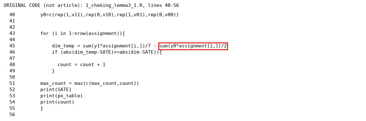
First, the proof of Lemma B.5 writes the mass function of the sum as g(x)=(f1(x)+f1(x−1))/2g(x)=(f_1(x)+f_1(x-1))/2. This is the convolution formula for independent variables, but the statement does not assume that X1X_1 and X2X_2 are independent, and without independence the conclusion can fail. Second, the proof takes the centre aa of mX1mX_1 to be an integer. A distribution that is SD on Z\mathbb Z can be centred at a half-integer, and such centres occur where the lemma is applied, in case 1 of the proof of Lemma B.6. The last sentence of the proof, on b=a+1/2b=a+1/2, concerns exactly this case, because bb is an integer. Third, the proof of Lemma B.9 applies Lemma B.5 to a conditional distribution that Lemma B.7 describes as SD on a lattice of spacing two. Such a distribution has no mass on the other half of the lattice (m−1)−1Z(m-1)^{-1}\mathbb Z and need not be SD on that lattice. The hypothesis of Lemma B.5 is then not met.
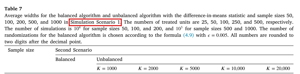

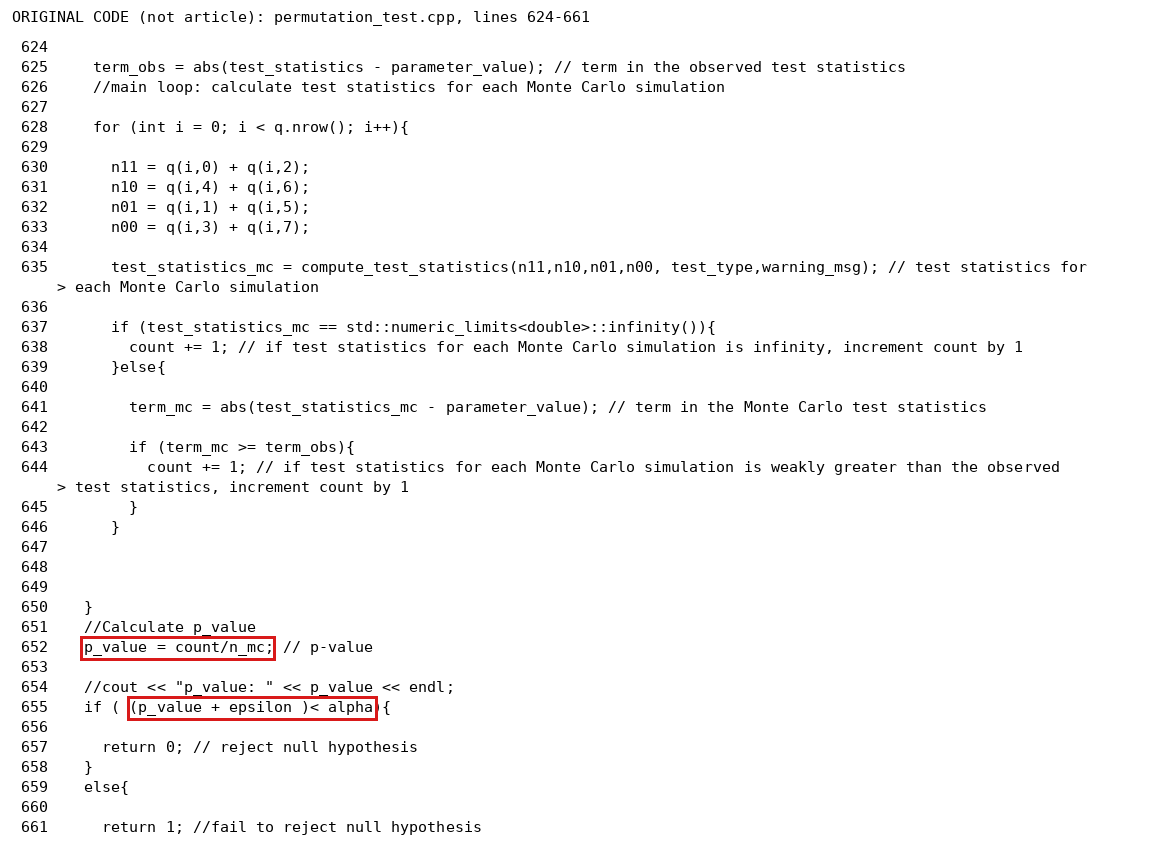
In each place the intended statement is true. The variables are independent where the lemma is applied, the proof of Lemma B.5 goes through for half-integer centres, and if an independent variable that is uniform on two adjacent points is added to an SD distribution on a lattice of spacing two, the sum is SD on the full lattice.

Evidence an exact counterexample

The evidence consists of exact counterexamples to the three printed steps and derivations of the corrected statements.

For the first error, let m=1m=1, let X1X_1 be uniform on {0,1}\{0,1\}, and set X2=X1X_2=X_1. Then X1X_1 is SD on Z\mathbb Z and X2X_2 is uniform on {0,1}\{0,1\}, but X1+X2X_1+X_2 takes the values 00 and 22 with probability 1/21/2 each and has no mass at its mean 11. For the second, let n=6n=6, m=3m=3 and v=(1,4,0,1)\mathbf v=(1,4,0,1). Removing a=(1,1,0,0)\mathbf a=(1,1,0,0) leaves (0,3,0,1)(0,3,0,1), for which (m−1)T(m-1)T takes the values 11 and 22 with probability 1/21/2 each, with centre 3/23/2. For the third, let n=4n=4, m=2m=2 and v=(1,1,0,2)\mathbf v=(1,1,0,2), and pair the subject of type (1,0)(1,0) with a subject of type (0,0)(0,0). The remaining table (1,0,0,1)(1,0,0,1) has (m−1)T(m-1)T uniform on {−1,1}\{-1,1\}, which is SD on 2Z+12\mathbb Z+1 and not on Z\mathbb Z.

For the corrected Lemma B.5, let ff be the mass function of mX1mX_1, symmetric about a point aa such that 2a2a is an integer. By independence, the mass function of m(X1+X2)m(X_1+X_2) is g(x)=(f(x)+f(x−1))/2g(x)=(f(x)+f(x-1))/2. Set c=a+1/2c=a+1/2. Using the symmetry of ff about aa, I obtain

g(2c−x)=12(f(2a+1−x)+f(2a−x))=12(f(x−1)+f(x))=g(x).g(2c-x)=\tfrac12\bigl(f(2a+1-x)+f(2a-x)\bigr)=\tfrac12\bigl(f(x-1)+f(x)\bigr)=g(x).

Let b≥cb\ge c be an integer and set t=b−a≥1/2t=b-a\ge1/2. Then ∣t−1∣≤t+1|t-1|\le t+1. By the SD property, I have f(b−1)≥f(b+1)f(b-1)\ge f(b+1), which gives

g(b)−g(b+1)=12(f(b−1)−f(b+1))≥0.g(b)-g(b+1)=\tfrac12\bigl(f(b-1)-f(b+1)\bigr)\ge0.

Together with the symmetry, this shows that m(X1+X2)m(X_1+X_2) is SD on Z\mathbb Z.

For the step in Lemma B.9, let YY be SD on 2Z+p2\mathbb Z+p with p∈{0,1}p\in\{0,1\}, with mass function ff and centre aa, and let UU be independent of YY and uniform on {0,1}\{0,1\}. Reflection about aa maps each point of the support to a point of the support, and both lie in 2Z+p2\mathbb Z+p. It follows that aa is an integer. The mass function of Y+UY+U is again g(x)=(f(x)+f(x−1))/2g(x)=(f(x)+f(x-1))/2, and it is symmetric about a+1/2a+1/2 by the computation above. Let b≥a+1b\ge a+1 be an integer. If b−pb-p is even, then b−1b-1 and b+1b+1 lie outside 2Z+p2\mathbb Z+p, and g(b)−g(b+1)=0g(b)-g(b+1)=0. If b−pb-p is odd, then b−1b-1 and b+1b+1 lie in 2Z+p2\mathbb Z+p and b+1>b−1≥ab+1>b-1\ge a. The SD property implies that f(b−1)≥f(b+1)f(b-1)\ge f(b+1), and hence g(b)≥g(b+1)g(b)\ge g(b+1). I conclude that Y+UY+U is SD on Z\mathbb Z.

What survives

Lemmas B.5, B.6 and B.9 hold with these changes. No hypothesis is added where the lemmas are used, because in the proofs of Lemmas B.6 and B.9 the pair and the remaining n−2n-2 subjects are randomized independently. Lemma B.12, Lemma 4.2, Theorem 4.1, the algorithms and the reported numbers are unchanged. Section 3 does not use these lemmas.

Corrected

“Lemma B.5. Let X1X_1 be SD on m−1Zm^{-1}\mathbb Z, and let X2X_2 be independent of X1X_1 and uniformly distributed on {0,m−1}\{0,m^{-1}\}. Then X1+X2X_1+X_2 is SD on m−1Zm^{-1}\mathbb Z.”

In the proof: “Suppose that mX1mX_1 is symmetric about a∈12Z\colorbox{#ffe58a}{$a\in\tfrac12\mathbb Z$}. […] it suffices to show that for any integer b≥a+1/2b\ge a+1/2, we have g(b)≥g(b+1)g(b)\ge g(b+1).”

In the proof of Lemma B.9, the citation of Lemma B.5 is replaced by the following statement: let YY be SD on 2Z+p2\mathbb Z+p for some p∈{0,1}p\in\{0,1\}, and let UU be independent of YY and uniformly distributed on {0,1}\{0,1\}; then Y+UY+U is SD on Z\mathbb Z. It is applied with Y=(m−1)T(v∘,Z′)Y=(m-1)T(\mathbf v^\circ,\mathbf Z') and with UU the signed contribution of the pair, so that mT(v,Z)=Y+UmT(\mathbf v,\mathbf Z)=Y+U. For the second form of v\mathbf v in (B.52), the signed contribution of the pair is U−1U-1 with UU uniform on {0,1}\{0,1\}, so that mT(v,Z)=Y+U−1mT(\mathbf v,\mathbf Z)=Y+U-1, and a shift by an integer preserves the SD property. When m=1m=1, there are no remaining subjects, and YY is taken to be 00.

Crop of Lemma B.5 and its proof, with display (B.43). Three red boxes: the words 'let X2 be uniformly distributed on {0, 1/m}' in the statement; 'a in Z' in the sentence 'Suppose that m X1 is symmetric about a in Z'; and 'If b = a + 1/2,' in the last sentence of the proof.
Appendix B.3, Lemma B.5 and its proof, p. 23 (PDF p. 23). The marked passages are the hypothesis on X2X_2, which does not mention independence, the restriction a∈Za\in\mathbb Z, and the case b=a+1/2b=a+1/2, which arises only for a half-integer aa. The citation of the lemma in the proof of Lemma B.9, on p. 25, is not shown.

The induction in the proof of Lemma B.12 should fix any v\mathbf v with v10+v01≥1v_{10}+v_{01}\ge1, compare v10+v01v_{10}+v_{01} with 2, and, when v10+v01>2v_{10}+v_{01}>2, require only that one of v10v_{10} and v01v_{01} be at least 2.

Appendix B.3, proof of Lemma B.12, p. 25 (PDF p. 25)

See also under Formal statements (Lean): P003-T15

As printed

“Lemma B.12. Let n=2mn=2m for some m∈Z>0m\in\mathbb Z_{>0}. Fix any potential outcome count vector

v=(v11,v10,v01,v00),(B.56)\mathbf v=(v_{11},v_{10},v_{01},v_{00}),\qquad\text{(B.56)}

and suppose v10+v01≥1v_{10}+v_{01}\ge1. Then the pmf of T(v,Z)T(\mathbf v,\mathbf Z) is SD on m−1Zm^{-1}\mathbb Z.

Proof. We induct on nn. The base case n=0n=0 is trivial. For the induction step, suppose that the claim is true for n−2n-2, and fix any v\mathbf v corresponding to a potential outcome table with nn subjects such that min⁡(v10,v01)≥1\colorbox{#ffe58a}{$\min(v_{10},v_{01})\ge1$}. If (v10,v01)=(1,0)(v_{10},v_{01})=(1,0) or (v10,v01)=(0,1)(v_{10},v_{01})=(0,1), we are done by Lemma B.9. If v01+v01=2\colorbox{#ffe58a}{$v_{01}+v_{01}$}=2, we are done by Lemma B.10 and Corollary B.11.

In the case v01+v01>2\colorbox{#ffe58a}{$v_{01}+v_{01}$}>2, we will use Lemma B.6 to show the claim is true for the given v\mathbf v. In this case, suppose first that v10≥2v_{10}\ge2 and v01≥1\colorbox{#ffe58a}{$v_{01}\ge1$}. Then by the induction hypothesis, Lemmas B.9, B.10, and Corollary B.11, the first condition given in the statement of Lemma B.6 holds. The case where v10≥1\colorbox{#ffe58a}{$v_{10}\ge1$} and v01≥2v_{01}\ge2 is analogous. This completes the proof.”

The problem

Lemma B.12 assumes only that v10+v01≥1v_{10}+v_{01}\ge1. The proof fixes v\mathbf v with min⁡(v10,v01)≥1\min(v_{10},v_{01})\ge1, and when the sum exceeds 2 it treats only the cases v10≥2v_{10}\ge2, v01≥1v_{01}\ge1 and v10≥1v_{10}\ge1, v01≥2v_{01}\ge2. Tables in which one of v10v_{10} and v01v_{01} is zero and the other is at least 3 satisfy the hypothesis of the lemma and fall under no case of the proof. The induction itself needs them: removing a=(0,1,1,0)\mathbf a=(0,1,1,0) from (0,4,1,1)(0,4,1,1) leaves (0,3,0,1)(0,3,0,1). The sum v01+v01v_{01}+v_{01} is printed twice where v10+v01v_{10}+v_{01} is meant. Read literally, the table (1,2,1,0)(1,2,1,0) has v01+v01=2v_{01}+v_{01}=2 and is sent to Lemma B.10 and Corollary B.11, which do not cover it. The lemma is true, and the lemmas already cited close the induction once the cases are stated correctly.

Evidence a historical Lean attribution (Generated status: clause support not certified in this release)

The evidence is a check of the page, a Lean proof of the arithmetic of the cases, an exact enumeration of the examples, and a derivation of the corrected induction. Here SD is read as in Definition A.1 with the corrections of P003-E006.

The table (0,4,0,0)(0,4,0,0), with n=4n=4, satisfies v10+v01≥1v_{10}+v_{01}\ge1 and lies outside the printed restriction, outside Lemma B.9, Lemma B.10 and Corollary B.11, and outside both cases with sum above 2. The same holds for (1,3,0,0)(1,3,0,0). Neither contradicts the lemma. For (0,4,0,0)(0,4,0,0), all six assignments give T=1T=1, and for (1,3,0,0)(1,3,0,0), three assignments give T=1/2T=1/2 and three give T=1T=1. The Lean proof covers these statements about the cases, and two facts used below. If v10+v01≥3v_{10}+v_{01}\ge3, then v10≥2v_{10}\ge2 or v01≥2v_{01}\ge2, and removing at most two of the subjects of types (1,0)(1,0) and (0,1)(0,1) leaves at least one of them.

For the corrected induction, set d=v10+v01≥1d=v_{10}+v_{01}\ge1. If d=1d=1, Lemma B.9 applies, and if d=2d=2, Lemma B.10 or Corollary B.11 applies. Suppose that d≥3d\ge3. Then n≥4n\ge4 and one of v10v_{10} and v01v_{01} is at least 2. If v10≥2v_{10}\ge2, every vector a\mathbf a in (B.45) removes at most two subjects of types (1,0)(1,0) and (0,1)(0,1). Each v−a\mathbf v-\mathbf a with nonnegative entries has n−2≥2n-2\ge2 subjects and satisfies the hypothesis of the lemma. By the induction hypothesis, the first condition of Lemma B.6 holds. If v01≥2v_{01}\ge2, the same argument with (B.46) shows that the second condition holds. No table with n=0n=0 satisfies v10+v01≥1v_{10}+v_{01}\ge1, and the base case holds vacuously.

What survives

Lemma B.12 holds as stated, with SD read as above. The proof of Lemma 4.2 applies it to v−(0,1,1,0)\mathbf v-(0,1,1,0), in which one of the two counts can be zero, and the corrected induction covers this case. Lemma 4.2, Theorem 4.1, the balanced algorithms and the reported numbers are unchanged.

Corrected

“Proof. We induct on nn. The base case n=0n=0 is trivial. For the induction step, suppose that the claim is true for n−2n-2, and fix any v\mathbf v corresponding to a potential outcome table with nn subjects such that v10+v01≥1\colorbox{#ffe58a}{$v_{10}+v_{01}\ge1$}. If (v10,v01)=(1,0)(v_{10},v_{01})=(1,0) or (v10,v01)=(0,1)(v_{10},v_{01})=(0,1), we are done by Lemma B.9. If v10+v01=2\colorbox{#ffe58a}{$v_{10}+v_{01}$}=2, we are done by Lemma B.10 and Corollary B.11.

In the case v10+v01>2\colorbox{#ffe58a}{$v_{10}+v_{01}$}>2, we will use Lemma B.6 to show the claim is true for the given v\mathbf v. In this case, at least one of v10v_{10} and v01v_{01} is at least 2. Suppose first that v10≥2v_{10}\ge2. For every a\mathbf a in (B.45) such that v−a\mathbf v-\mathbf a has nonnegative entries, the vector v−a\mathbf v-\mathbf a has n−2n-2 subjects, and the sum of its second and third entries is at least v10+v01−2≥1\colorbox{#ffe58a}{$v_{10}+v_{01}-2\ge1$}. Then by the induction hypothesis, the first condition given in the statement of Lemma B.6 holds. The case where v01≥2\colorbox{#ffe58a}{$v_{01}\ge2$} is analogous, with (B.46) and the second condition. This completes the proof.”

Crop of the last line of Lemma B.12, 'and suppose v10 + v01 is at least 1. Then the pmf of T(v, Z) is SD on the lattice of multiples of 1/m', its proof, and the one-line proof of Lemma 4.2. Six red boxes in the proof: 'min(v10, v01) is at least 1'; 'v01 + v01 = 2'; 'v01 + v01 greater than 2'; 'v10 at least 2' continued on the next line by 'and v01 at least 1'; and 'v10 at least 1 and v01 at least 2'.
Appendix B.3, end of the statement of Lemma B.12 and its proof, p. 25 (PDF p. 25). The marked conditions restrict the induction to tables with both v10v_{10} and v01v_{01} positive, although the lemma assumes only v10+v01≥1v_{10}+v_{01}\ge1; the sum v01+v01v_{01}+v_{01} is printed twice for v10+v01v_{10}+v_{01}.

In (B.47) and (B.49)–(B.51) the control outcomes are subtracted, not added, and the sums (B.50) and (B.51) carry the factor 1/m1/m.

Appendix B.3, displays (B.47), (B.49), (B.50) and (B.51), p. 24 (PDF p. 24), in the proofs of Lemmas B.6 and B.7

See also under Formal statements (Lean): P003-T16

As printed

Proof of Lemma B.6: “Then w1(1)−wj(0)=0w_1(1)-w_j(0)=0, and wj(1)−w1(0)=1w_j(1)-w_1(0)=1, so the distribution of

Z1w1(1)+(1−Z1)w1(0)+Zjwj(1)+(1−Zj)wj(0)(B.47)Z_1w_1(1)\colorbox{#ffe58a}{$\displaystyle +$}(1-Z_1)w_1(0)+Z_jw_j(1)\colorbox{#ffe58a}{$\displaystyle +$}(1-Z_j)w_j(0)\qquad\text{(B.47)}

is uniform on the set {0,1}\{0,1\}.”

Proof of Lemma B.7: “We consider first the case that w2=(1,1)\mathbf w_2=(1,1). Then the distribution of

Z1w1(1)+(1−Z1)w1(0)+Zjwj(1)+(1−Zj)wj(0)(B.49)Z_1w_1(1)\colorbox{#ffe58a}{$\displaystyle +$}(1-Z_1)w_1(0)+Z_jw_j(1)\colorbox{#ffe58a}{$\displaystyle +$}(1-Z_j)w_j(0)\qquad\text{(B.49)}

conditional on the choice of partner and that fact that subjects 1 and 2 are assigned to different groups is constant and equal to 0. This implies we are done by induction, since v11−2v_{11}-2, the number of (1,1)(1,1) potential outcome vectors in the remaining n−2n-2 subjects, has the same parity as v11v_{11}, and the sampling distributions of

∑i=1nZiwi(1)+(1−Zi)wi(0)(B.50)\sum_{i=1}^nZ_iw_i(1)\colorbox{#ffe58a}{$\displaystyle +$}(1-Z_i)w_i(0)\qquad\text{(B.50)}

and

∑i=3nZiwi(1)+(1−Zi)wi(0)(B.51)\sum_{i=3}^nZ_iw_i(1)\colorbox{#ffe58a}{$\displaystyle +$}(1-Z_i)w_i(0)\qquad\text{(B.51)}

are then both supported and SD on either m−1(2Z)m^{-1}(2\mathbb Z) or m−1(2Z+1)m^{-1}(2\mathbb Z+1), as desired.”

The problem

The four displays are contributions to the estimator TT of (2.7), in which control outcomes enter with a minus sign. The sentence before (B.47) uses the differences w1(1)−wj(0)w_1(1)-w_j(0) and wj(1)−w1(0)w_j(1)-w_1(0), and the distributions stated in the two proofs are those of the sums with minus signs. With the printed plus signs they are wrong. For w1=(1,0)\mathbf w_1=(1,0) and wj=(1,1)\mathbf w_j=(1,1), the printed sum (B.47) takes the values 22 and 11, not 00 and 11. For w1=wj=(1,1)\mathbf w_1=\mathbf w_j=(1,1), the printed sum (B.49) is the constant 22, not 00. The sums (B.50) and (B.51) are integers, and the claim that they are SD on m−1(2Z)m^{-1}(2\mathbb Z) or m−1(2Z+1)m^{-1}(2\mathbb Z+1) requires the factor 1/m1/m. The proof of Lemma B.7 also writes w2\mathbf w_2 for the partner that (B.49) calls wj\mathbf w_j, and (B.51) starts at i=3i=3. This is consistent once the partner is relabelled as subject 2, which the proof does not say.

Evidence a derivation

The evidence is a recalculation of the pair sums in every case of the two proofs. The two values in each cell correspond to (Z1,Zj)=(1,0)(Z_1,Z_j)=(1,0) and (0,1)(0,1).

Values of the pair sum, as printed and with the control outcomes subtracted, beside the distribution stated in the proof.
Types w1\mathbf w_1, wj\mathbf w_jPrinted sumSum with minus signsStated in the proof
(1,0)(1,0), (1,1)(1,1)22, 1100, 11uniform on {0,1}\{0,1\}
(1,0)(1,0), (1,0)(1,0)11, 1111, 11constant 11
(1,0)(1,0), (0,1)(0,1)22, 0000, 00constant 00
(1,0)(1,0), (0,0)(0,0)11, 0011, 00uniform on {0,1}\{0,1\}
(1,1)(1,1), (1,1)(1,1)22, 2200, 00constant 00
(1,1)(1,1), (0,0)(0,0)11, 1111, −1-1uniform on {−1,1}\{-1,1\}

For the normalization, let AA be the pair sum with minus signs and RR the corresponding sum over the remaining n−2n-2 subjects. By (2.7), I have T(v,Z)=(A+R)/mT(\mathbf v,\mathbf Z)=(A+R)/m, and, when m>1m>1, the estimator for the remaining subjects is R/(m−1)R/(m-1). The remaining subjects contribute R/mR/m to TT, and this contribution lies in m−1Zm^{-1}\mathbb Z; when m=1m=1, the empty sum is R=0R=0.

What survives

Lemmas B.6 and B.7 hold, and their proofs go through with the corrected displays. Nothing else in the paper changes.

Corrected
Z1w1(1)−(1−Z1)w1(0)+Zjwj(1)−(1−Zj)wj(0)(B.47), (B.49)Z_1w_1(1)\colorbox{#ffe58a}{$\displaystyle -$}(1-Z_1)w_1(0)+Z_jw_j(1)\colorbox{#ffe58a}{$\displaystyle -$}(1-Z_j)w_j(0)\qquad\text{(B.47), (B.49)}
1m∑i=1n[Ziwi(1)−(1−Zi)wi(0)](B.50)\colorbox{#ffe58a}{$\displaystyle \frac1m$}\sum_{i=1}^n\bigl[Z_iw_i(1)\colorbox{#ffe58a}{$\displaystyle -$}(1-Z_i)w_i(0)\bigr]\qquad\text{(B.50)}
1m∑i=3n[Ziwi(1)−(1−Zi)wi(0)](B.51)\colorbox{#ffe58a}{$\displaystyle \frac1m$}\sum_{i=3}^n\bigl[Z_iw_i(1)\colorbox{#ffe58a}{$\displaystyle -$}(1-Z_i)w_i(0)\bigr]\qquad\text{(B.51)}

The sums (B.47) and (B.49) keep the integer-valued distributions stated in the proofs, and they are divided by mm when they are combined with the remaining subjects to form TT. In the proof of Lemma B.7, after the partner is chosen: “Conditional on the choice of partner, the partner is relabelled as subject 2, so that j=2\colorbox{#ffe58a}{$j=2$}.”

Crop of the first case in the proof of Lemma B.7. Six red boxes: the symbol w2 in 'We consider first the case that w2 = (1,1)'; the plus signs before (1 - Z1) w1(0) and before (1 - Zj) wj(0) in display (B.49); the plus sign before (1 - Zi) wi(0) in displays (B.50) and (B.51); and the words 'm inverse (2Z) or m inverse (2Z + 1)' in the sentence that follows the displays.
Appendix B.3, proof of Lemma B.7, p. 24 (PDF p. 24), displays (B.49)–(B.51). The marked plus signs stand before the control outcomes, which the estimator subtracts. The partner is called w2\mathbf w_2 in the text and wj\mathbf w_j in (B.49), and the marked lattices require the sums (B.50) and (B.51) to be divided by mm. Display (B.47), earlier on the page, has the same two plus signs.

In the proof of Proposition 3.2, the threshold xx should be the smallest value of the absolute deviation whose tail probability is below α\alpha, if such a value exists; a smallest real number with that property does not exist.

Appendix A.2, proof of Proposition 3.2, p. 19 (PDF p. 19), the sentence that introduces (A.10)

See also under Formal statements (Lean): P003-T11, P003-T12, P003-T29

As printed

“Here probability is with respect to Z~\widetilde{\mathbf Z}, and we consider the left side of (A.9) as a function of T(Y,Z)T(\mathbf Y,\mathbf Z). Let xx denote the smallest real number such that

P(∣T(Y~,Z~)−τ(y)∣≥x)<α,(A.10)\mathbb P\Bigl(\bigl|T(\widetilde{\mathbf Y},\widetilde{\mathbf Z})-\tau(\mathbf y)\bigr|\ge x\Bigr)<\alpha,\qquad\text{(A.10)}

which exists because T(Y~,Z~)T(\widetilde{\mathbf Y},\widetilde{\mathbf Z}) is a discrete random variable supported on a bounded set. Then the event where (A.9) occurs is the same as the event where ∣T(Y,Z)−τ(y)∣≥x\bigl|T(\mathbf Y,\mathbf Z)-\tau(\mathbf y)\bigr|\ge x. By the definition of xx, and the fact that (Y,Z)(\mathbf Y,\mathbf Z) and (Y~,Z~)(\widetilde{\mathbf Y},\widetilde{\mathbf Z}) are identically distributed, this event has probability at most α\alpha. This completes the proof.”

The problem

Let D=∣T(Y~,Z~)−τ(y)∣D=|T(\widetilde{\mathbf Y},\widetilde{\mathbf Z})-\tau(\mathbf y)| and q(t)=P(D≥t)q(t)=\mathbb P(D\ge t). The variable DD takes finitely many values, and the set of real numbers tt such that q(t)<αq(t)<\alpha is an open half-line (d,∞)(d,\infty), where dd is the largest value of DD such that q(d)≥αq(d)\ge\alpha. This set has no smallest element. The number xx is therefore not defined, and the two sentences that use it do not prove the claim. The error is confined to this step, and Proposition 3.2 holds as stated.

Evidence a historical Lean attribution (Generated status: clause support not certified in this release)

The evidence is an exact counterexample to the existence of xx, with a Lean proof of its statement about real thresholds, and a derivation of the corrected step.

For the counterexample, let n=2n=2, m=1m=1, α=1/2\alpha=1/2 and y1=y2=(0,0)y_1=y_2=(0,0). Both assignments give Y=(0,0)\mathbf Y=(0,0) and T(Y,Z)=0=τ(y)T(\mathbf Y,\mathbf Z)=0=\tau(\mathbf y). Then D=0D=0 with probability one, and I have q(t)=1q(t)=1 for t≤0t\le0 and q(t)=0q(t)=0 for t>0t>0. The real numbers tt such that q(t)<1/2q(t)<1/2 are the positive numbers, and if tt is one of them, then so is t/2t/2. A Lean proof establishes that this set is (0,∞)(0,\infty), that it has no smallest element, and that t=0t=0 does not satisfy the strict inequality. The coverage claim is not violated in this example, since the interval is [−1/2,1/2][-1/2,1/2] for both assignments.

In general, let d1<⋯<dkd_1<\dots<d_k be the values of DD, and let rr be the largest index such that q(dr)≥αq(d_r)\ge\alpha, which exists because q(d1)=1q(d_1)=1. For t≤drt\le d_r, I have q(t)≥q(dr)≥αq(t)\ge q(d_r)\ge\alpha. For t>drt>d_r, every value of DD that is at least tt has index at least r+1r+1, and I have q(t)≤q(dr+1)<αq(t)\le q(d_{r+1})<\alpha if r<kr<k, and q(t)=0q(t)=0 if r=kr=k. I conclude that {t:q(t)<α}=(dr,∞)\{t:q(t)<\alpha\}=(d_r,\infty).

For the corrected step, let S={d1,…,dk}S=\{d_1,\dots,d_k\} and R={d∈S:q(d)<α}R=\{d\in S:q(d)<\alpha\}. Let D0=∣T(Y,Z)−τ(y)∣D_0=|T(\mathbf Y,\mathbf Z)-\tau(\mathbf y)| be the observed deviation, which takes values in SS and has the same distribution as DD. The event in (A.9) is {q(D0)<α}\{q(D_0)<\alpha\}. If RR is empty, this event is empty. Otherwise, set x=min⁡Rx=\min R. For d∈Sd\in S with d<xd<x, I have q(d)≥αq(d)\ge\alpha, since d∉Rd\notin R. For d∈Sd\in S with d≥xd\ge x, I have q(d)≤q(x)<αq(d)\le q(x)<\alpha. The event in (A.9) is then {D0≥x}\{D_0\ge x\}, and its probability is q(x)<αq(x)<\alpha.

What survives

Proposition 3.2 holds under its stated hypotheses, including unbalanced designs. The number xx appears only in this proof, and no algorithm computes it. The correction changes no interval, no bound and no reported number. The same argument with R={d∈S:q(d)≤α}R=\{d\in S:q(d)\le\alpha\} covers the acceptance rule p>αp>\alpha of footnote 8.

Corrected

“Here probability is with respect to Z~\widetilde{\mathbf Z}, and we consider the left side of (A.9) as a function of T(Y,Z)T(\mathbf Y,\mathbf Z). Let SS be the finite set of values of ∣T(Y~,Z~)−τ(y)∣\bigl|T(\widetilde{\mathbf Y},\widetilde{\mathbf Z})-\tau(\mathbf y)\bigr|. If no x∈Sx\in S satisfies (A.10) below, the event where (A.9) occurs is empty. Otherwise, let xx denote the smallest element of SS such that

P(∣T(Y~,Z~)−τ(y)∣≥x)<α.(A.10)\mathbb P\Bigl(\bigl|T(\widetilde{\mathbf Y},\widetilde{\mathbf Z})-\tau(\mathbf y)\bigr|\ge x\Bigr)<\alpha.\qquad\text{(A.10)}

Then the event where (A.9) occurs is the same as the event where ∣T(Y,Z)−τ(y)∣≥x\bigl|T(\mathbf Y,\mathbf Z)-\tau(\mathbf y)\bigr|\ge x. Since (Y,Z)(\mathbf Y,\mathbf Z) and (Y~,Z~)(\widetilde{\mathbf Y},\widetilde{\mathbf Z}) are identically distributed, the probability of this event is the left side of (A.10), which is less than α\alpha. This completes the proof.”

Crop of the proof of Proposition 3.2, with displays (A.9) and (A.10). A red box, split over two lines, marks the words 'smallest real number such that' in the sentence 'Let x denote the smallest real number such that', which is followed by display (A.10): the probability that the absolute value of T minus tau(y) is at least x is less than alpha.
Appendix A.2, proof of Proposition 3.2, p. 19 (PDF p. 19). The marked words define xx as the smallest real number that satisfies (A.10).

The studentized statistic (5.8) has no value when σ(n)=0\sigma(\mathbf n)=0, and footnote 13 does not cover it; a fixed finite value must be assigned in that case and used for the observed and the simulated assignments alike.

Section 5.1, equations (5.8)–(5.11), p. 11 (PDF p. 11); footnote 13, p. 11

See also under Formal statements (Lean): P003-T17

As printed

“For inference on τ\tau, we could also use the studentized test statistic

Rstd(n,v)=T(n)−τ(v)σ(n),(5.8)R_{\mathrm{std}}(\mathbf n,\mathbf v)=\frac{T(\mathbf n)-\tau(\mathbf v)}{\colorbox{#ffe58a}{$\displaystyle \sigma(\mathbf n)$}},\qquad\text{(5.8)}

where

σ2(n)=Q1(n11+n10)2+Q0(n01+n00)2,(5.9)\sigma^2(\mathbf n)=\frac{Q_1}{(n_{11}+n_{10})^2}+\frac{Q_0}{(n_{01}+n_{00})^2},\qquad\text{(5.9)}
Q1=n11(n11n11+n10−1)2+n10(n11n11+n10)2,(5.10)Q_1=n_{11}\left(\frac{n_{11}}{n_{11}+n_{10}}-1\right)^2+n_{10}\left(\frac{n_{11}}{n_{11}+n_{10}}\right)^2,\qquad\text{(5.10)}
Q0=n01(n01n01+n00−1)2+n00(n01n01+n00)2.(5.11)Q_0=n_{01}\left(\frac{n_{01}}{n_{01}+n_{00}}-1\right)^2+n_{00}\left(\frac{n_{01}}{n_{01}+n_{00}}\right)^2.\qquad\text{(5.11)}

The function σ2\sigma^2 is the usual variance estimator written in terms of n\mathbf n.”

Footnote 13, attached to the risk-ratio statistic RRRR_{\mathrm{RR}} that follows: “In each of these expressions (and the ones in the next example), we interpret division by zero as returning some arbitrarily selected real number, such as 10610^6. This case is rare: as long as one treated unit has outcome 0 and one control unit has outcome 1, (5.12) and (5.13) will have nonzero denominators.”

The problem

Section 5.1 defines a test statistic as a real-valued function of (n,v)(\mathbf n,\mathbf v), and the design allows every potential outcome table (2.1). Expanding (5.10) and (5.11), I obtain Q1=n11n10/(n11+n10)Q_1=n_{11}n_{10}/(n_{11}+n_{10}) and Q0=n01n00/(n01+n00)Q_0=n_{01}n_{00}/(n_{01}+n_{00}). This implies that σ(n)=0\sigma(\mathbf n)=0 exactly when n11n10=0n_{11}n_{10}=0 and n01n00=0n_{01}n_{00}=0, that is, when the observed outcomes are constant within each arm. For such data (5.8) is 0/00/0, or a nonzero number divided by zero. Footnote 13 is attached to the risk-ratio example and extends to “the next example”, the odds ratio; it does not reach back to (5.8). Algorithms 5.1 and 5.3 and Theorem 5.5 take a real-valued statistic. They do not apply to RstdR_{\mathrm{std}} as printed until a value is fixed for this case.

Evidence an exact counterexample

The evidence is an exact counterexample, found by enumerating every assignment. Let n=5n=5 and m=2m=2. Suppose that all five subjects have potential outcomes (0,0)(0,0). For each of the 10 assignments, I have n=(0,2,0,3)\mathbf n=(0,2,0,3), T=0T=0, Q1=Q0=0Q_1=Q_0=0 and τ=0\tau=0, and (5.8) is 0/00/0 with probability one. If one subject has outcomes (0,1)(0,1) and the other four have (0,0)(0,0), then τ=−1/5\tau=-1/5, and in the 4 of 10 assignments that treat this subject the numerator is 1/51/5 and σ=0\sigma=0.

The repair keeps (5.4). If one real-valued function is applied to the observed assignment and to the KK simulated ones, the K+1K+1 values are exchangeable under the null. Let rir_i be the number of these values that are at least as large in absolute value as the iith one, so that S=r0/(K+1)S=r_0/(K+1) in (5.3). For every integer t≥0t\ge0, at most tt indices have ri≤tr_i\le t, ties included. Taking t=⌊α(K+1)⌋t=\lfloor\alpha(K+1)\rfloor, I obtain P(S≤α)≤⌊α(K+1)⌋/(K+1)≤α\mathbb P(S\le\alpha)\le\lfloor\alpha(K+1)\rfloor/(K+1)\le\alpha. The constant matters for the test itself: in the second example, the exact pp-value of the true table at the all-zero observation is 11 if the assigned value is 00 and 2/52/5 if it is 10610^6.

What survives

Remark 5.2 and Theorem 5.5 hold for every real-valued statistic, and in particular for RstdR_{\mathrm{std}} once the value at σ(n)=0\sigma(\mathbf n)=0 is fixed. The procedures based on the difference in means, the balanced algorithms and the missing-data construction do not use (5.8). In the six populations simulated for Table 3, the variance estimate is positive under every assignment. The true table never meets this case there, but other tables tested during the inversion can. No reported number is shown to change.

Corrected

“For inference on τ\tau, we could also use the studentized test statistic

Rstd(n,v)={T(n)−τ(v)σ(n),σ(n)>0,C,σ(n)=0,(5.8)R_{\mathrm{std}}(\mathbf n,\mathbf v)= \begin{cases} \dfrac{T(\mathbf n)-\tau(\mathbf v)}{\sigma(\mathbf n)}, & \sigma(\mathbf n)>0,\\[6pt] {}\colorbox{#ffe58a}{$\displaystyle C$}, & {}\colorbox{#ffe58a}{$\displaystyle \sigma(\mathbf n)=0,$} \end{cases} \qquad\text{(5.8)}

where σ(n)≥0\sigma(\mathbf n)\ge 0 is defined by (5.9)–(5.11) for count vectors n\mathbf n with both arms nonempty, and CC is a finite real constant, such as 10610^6, fixed before the tests are run. The same function is applied to the observed assignment and to every simulated or reused assignment.”

Crop of the bullet 'For inference on tau, we could also use the studentized test statistic' with equations (5.8) to (5.11) and the sentence 'The function sigma squared is the usual variance estimator written in terms of n.' A red box marks the denominator sigma(n) of equation (5.8), R_std(n, v) = (T(n) - tau(v))/sigma(n).
Equations (5.8)–(5.11), p. 11 (PDF p. 11). The marked denominator σ(n)\sigma(\mathbf n) is zero whenever the observed outcomes are constant within each arm.
Crop of the two lines of footnote 13. A red box marks the opening words 'In each of these expressions (and the ones in the next example)'. The footnote continues: 'we interpret division by zero as returning some arbitrarily selected real number, such as 10 to the power 6. This case is rare: as long as one treated unit has outcome 0 and one control unit has outcome 1, (5.12) and (5.13) will have nonzero denominators.'
Footnote 13, p. 11 (PDF p. 11), attached to the risk-ratio statistic after (5.13). The marked words limit the convention on division by zero to the risk-ratio expressions and to the next example, the odds ratio.

The operation count of the balanced algorithm is O(n2 polylog(n))O(n^2\,\mathrm{polylog}(n)) for fixed ϵ\epsilon, as in (1.6), not O(n×polylog(n))O(n\times\mathrm{polylog}(n)); and the choice of KK in (4.9) has log⁡2n\log_2 n, not log⁡2n\log^2 n.

Remark 5.7, second sentence, p. 13 (PDF p. 13); compare (1.6), p. 4, and (4.9), p. 9

See also under Formal statements (Lean): P003-T18

As printed

“The time-complexity of the balanced algorithm is O(n×polylog(n))O(\colorbox{#ffe58a}{$n$}\times\mathrm{polylog}(n)), by choosing K=log⁡(4nlog⁡2n/ϵ)/(2ϵ2)K=\log(4n\colorbox{#ffe58a}{$\log^2 n$}/\epsilon)/(2\epsilon^2) (following (4.9)), and for the unbalanced algorithm, the time complexity is O(Kn3)O(Kn^3).”

The problem

The paper measures run time in arithmetic operations (p. 4, footnote 7), and a Monte Carlo test with KK samples costs O(Kn)O(Kn) operations when the assignments are generated by the Fisher–Yates algorithm (p. 13). By Theorem 4.1, there are O(nlog⁡n)O(n\log n) tests, and (4.9) implies that KK is of order log⁡n\log n for fixed ϵ\epsilon. The product is O(n2log⁡2n)O(n^2\log^2 n), which is the bound (1.6). The order n polylog(n)n\,\mathrm{polylog}(n) printed in the remark is that of the number of Monte Carlo draws, O(Knlog⁡n)O(Kn\log n). The bound O(Kn3)O(Kn^3) for the unbalanced algorithm is a number of operations. The remark also has log⁡2n\log^2 n inside KK where (4.9) has log⁡2n\log_2 n.

Evidence an exact counterexample

The evidence is a derivation of the upper bound and an exact family of executions that excludes the printed order. For the upper bound, I multiply the O(nlog⁡n)O(n\log n) tests of Theorem 4.1 by the O(Kn)O(Kn) operations of one test and insert K=⌈log⁡(4nlog⁡2n/ϵ)/(2ϵ2)⌉K=\lceil\log(4n\log_2 n/\epsilon)/(2\epsilon^2)\rceil, which is of order log⁡n\log n for fixed 0<ϵ<α0<\epsilon<\alpha. This gives O(n2log⁡2n)O(n^2\log^2 n).

For the lower bound, let n=2rn=2^r with r≥4r\ge 4, m=n/2m=n/2, α=1/2\alpha=1/2 and ϵ=1/8\epsilon=1/8, and let every observed outcome be zero, so that n=(0,m,0,m)\mathbf n=(0,m,0,m). The first query of the search for the upper endpoint in Algorithm 4.3 is τ0=1/4\tau_0=1/4. At this query the possible tables are vj=(0,j,j−n/4,n−2j+n/4)\mathbf v_j=(0,j,j-n/4,n-2j+n/4) for n/4≤j≤n/2n/4\le j\le n/2, and there are n/4+1n/4+1 tests if all of them reject. For each vj\mathbf v_j there exists an assignment such that V=0V=0 in (4.6), since its statistic equals τ0\tau_0. If every draw is this assignment, then S=0S=0 and the test rejects, for every KK. On this event the first query alone takes (n/4+1)K(n−1)(n/4+1)K(n-1) iterations of the Fisher–Yates shuffle. For n=16n=16 this is 5 tests and, with K=244K=244 as in (4.9), 1220 draws and 18300 iterations. More generally, by Chebyshev’s inequality each exact pp-value is at most 4/(n−1)4/(n-1); a concentration bound and a union bound show that, for r≥6r\ge 6 and KK as in (4.9), all n/4+1n/4+1 tests reject with probability greater than 1/21/2. I conclude that the expected number of operations is at least of order n2log⁡nn^2\log n, which is not O(n polylog(n))O(n\,\mathrm{polylog}(n)).

The squared logarithm does not endanger coverage. Since log⁡2n/log⁡2n=log⁡n log⁡2>1\log^2 n/\log_2 n=\log n\,\log 2>1 for n≥15n\ge 15, the printed KK is larger than (4.9) requires, and it has the same order.

What survives

The bound (1.6), Theorem 4.1, Proposition 4.6 and the coverage results do not depend on the remark. Its conclusion also stands: for fixed ϵ\epsilon the corrected bound for the balanced algorithm is of smaller order than n3n^3, against O(Kn3)O(Kn^3) for the unbalanced one. The timings of Tables 4 and 5 were measured and do not use the sentence. The corrected bound is weaker than the printed one. It concerns the implementation that the paper analyzes, which generates each assignment by a shuffle, and it says nothing about an implementation that samples counts directly, as the released code does.

Corrected

“The time-complexity of the balanced algorithm, for fixed 0<ϵ<α\colorbox{#ffe58a}{$0<\epsilon<\alpha$}, is O(n2×polylog(n))O(\colorbox{#ffe58a}{$n^2$}\times\mathrm{polylog}(n)) (more precisely O(n2log⁡2n)\colorbox{#ffe58a}{$O(n^2\log^2 n)$}), by choosing K=⌈log⁡(4nlog⁡2n/ϵ)/(2ϵ2)⌉K=\colorbox{#ffe58a}{$\lceil$}\log(4n\colorbox{#ffe58a}{$\log_2 n$}/\epsilon)/(2\epsilon^2)\colorbox{#ffe58a}{$\rceil$} (following (4.9)), and for the unbalanced algorithm, the time complexity is O(Kn3)O(Kn^3).”

Crop of the six lines of Remark 5.7. Red boxes mark 'O(n x polylog(n))' in 'The time-complexity of the balanced algorithm is O(n x polylog(n))' and 'log^2 n' inside the formula K = log(4n log^2 n / epsilon)/(2 epsilon^2). The sentence continues '(following (4.9)), and for the unbalanced algorithm, the time complexity is O(K n^3). Hence, for large n, the balanced algorithm will be more efficient than the unbalanced algorithm.'
Remark 5.7, p. 13 (PDF p. 13). The first marked term is the stated run time of the balanced algorithm, which lacks a factor of nn; the second is the squared logarithm in KK, where (4.9) has the logarithm to base 2.

With a known binary covariate, the eight counts satisfy two linear restrictions, one for each stratum size, and not the single restriction of footnote 16; the number of count vectors is O(n6)O(n^6), and the printed O(n7)O(n^7) and O(n6)O(n^6) are valid but loose upper bounds.

Section 8, paragraph beginning “To understand the difficulty that strata create”, and footnote 16, p. 17 (PDF p. 17)

See also under Formal statements (Lean): P003-T19

As printed

“[…] with an additional degree of freedom coming from the new binary covariate, increasing the number of potential outcome count vectors v\mathbf{v} to examine from O(n3)O(n^3) to O(n7)O(n^7).”

Footnote 16: “Without the covariate, there are 4 coordinates to choose from, with the single linear restriction that they sum to nn. With the binary covariate, there are 8 coordinates and a single linear restriction.”

Next paragraph: “One can similarly gain a factor of nn when there is a binary covariate, but this only brings the time complexity to O(n6)O(n^6), which is far from practical.”

The problem

In the experiment of this paragraph, the subjects with X=0X = 0 and the subjects with X=1X = 1 are randomized separately. Since the covariate of every subject is known, the numbers N0N_0 and N1N_1 of subjects in the two strata are fixed. A potential outcome table can change the outcomes of a subject but not its stratum. The four counts within each stratum then sum to the size of that stratum. The eight counts satisfy two independent linear restrictions, and six of them are free. Footnote 16 states a single restriction, which is the sum of these two. The count that the footnote supports is one power of nn too large: there are O(n6)O(n^6) count vectors, and the bound O(n7)O(n^7) in the text is valid but not sharp. The next paragraph inherits the extra power. If the Monte Carlo draws are reused as in Section 5, the running time is equivalent to O(n5)O(n^5) approximate permutation tests. The printed O(n6)O(n^6) is an upper bound for the cost of that approach and not its order.

Evidence an exact counterexample

The evidence is a derivation and an exact enumeration. I write vabsv_{abs} for the number of subjects with X=sX = s and potential outcomes (w(1),w(0))=(a,b)(w(1), w(0)) = (a, b). Each subject of stratum ss has exactly one pair (a,b)(a, b), so

v110+v100+v010+v000=N0,v111+v101+v011+v001=N1.v_{110} + v_{100} + v_{010} + v_{000} = N_0, \qquad v_{111} + v_{101} + v_{011} + v_{001} = N_1 .

The two equations involve disjoint sets of counts and are independent, and their sum is the restriction that the eight counts sum to nn. The four counts of stratum ss range over the (Ns+33)\binom{N_s+3}{3} nonnegative integer solutions of the corresponding equation. Each solution is realized by some table, and the two strata are chosen independently. Before the observed outcomes are used, the number of count vectors is

(N0+33)(N1+33)≤(n+3)636=O(n6),\binom{N_0+3}{3}\binom{N_1+3}{3} \le \frac{(n+3)^6}{36} = O(n^6),

and it is at least c6n6/36c^6 n^6/36 when N0≥cnN_0 \ge cn and N1≥cnN_1 \ge cn for a constant c>0c > 0. With the single restriction of the footnote, the count is (n+77)\binom{n+7}{7}, of order n7/5040n^7/5040, and it includes vectors with other stratum sizes. For n=4n = 4 and N0=N1=2N_0 = N_1 = 2, there are 330 nonnegative integer vectors with sum 4, and 100 of them have both stratum sums equal to 2. These 100 are the count vectors of the 44=2564^4 = 256 tables. The vector (3,0,0,0;1,0,0,0)(3,0,0,0;1,0,0,0) satisfies the restriction of the footnote and is the count vector of no table.

For the running time, I split the count vectors of stratum 0 into lines. Along a line, consecutive vectors differ by (−1,+1,+1,−1)(-1, +1, +1, -1) in the order (v110,v100,v010,v000)(v_{110}, v_{100}, v_{010}, v_{000}). There are at most (N0+1)(2N0+1)(N_0+1)(2N_0+1) lines, and each has at most N0+1N_0 + 1 vectors. With the counts of stratum 1 held fixed, I obtain at most

(N0+1)(2N0+1)(N1+33)=O(n5)(N_0+1)(2N_0+1)\binom{N_1+3}{3} = O(n^5)

lines in all. Along a line, the KK draws are updated in O(K)O(K) operations per vector, as in Section 5.1.1 applied within stratum 0. A line then costs O(Kn)O(Kn) operations, and the whole computation costs O(Kn6)O(Kn^6). Since one Monte Carlo permutation test with KK samples costs O(Kn)O(Kn), this is equivalent to O(n5)O(n^5) tests. Both figures are upper bounds, and no lower bound is claimed.

What survives

The correction concerns the discussion of future work in Section 8 and needs no new assumption, since the stratum sizes are part of the stated design. The printed O(n7)O(n^7) and O(n6)O(n^6) remain valid upper bounds. The algorithms and results of Sections 3–6 and the examples and simulations of Section 7 concern complete randomization without strata and do not use this count. The interest in more efficient methods for stratified designs is unchanged.

Corrected

Footnote 16: “Without the covariate, there are 4 coordinates to choose from, with the single linear restriction that they sum to nn. With the binary covariate, there are 8 coordinates and two linear restrictions: the four counts for the subjects with X=0X = 0 sum to the number N0N_0 of these subjects, and the four counts for the subjects with X=1X = 1 sum to the number N1N_1 of these subjects. Before compatibility with the observed outcomes is imposed, there are (N0+33)(N1+33)=O(n6)\binom{N_0+3}{3}\binom{N_1+3}{3} = O(n^6) count vectors, and this order is attained when N0N_0 and N1N_1 are both proportional to nn.”

In the text, the bounds may stand as loose upper bounds, or they may be sharpened: “[…] increasing the number of potential outcome count vectors v\mathbf{v} to examine from O(n3)O(n^3) to O(n6)\colorbox{#ffe58a}{$O(n^6)$}”, and, in the next paragraph, “One can similarly gain a factor of nn when there is a binary covariate, which brings the running time to the equivalent of O(n5)\colorbox{#ffe58a}{$O(n^5)$} approximate permutation tests, or O(Kn6)O(Kn^6) arithmetic operations […]”.

Crop of footnote 16, two lines under a short rule: Without the covariate, there are 4 coordinates to choose from, with the single linear restriction that they sum to n. With the binary covariate, there are 8 coordinates and a single linear restriction. A red outline surrounds the last words: a single linear restriction.
Footnote 16, p. 17. The outline marks the statement that the eight counts satisfy a single linear restriction.
Crop of two paragraphs of Section 8. The first begins: To understand the difficulty that strata create, suppose that each subject comes equipped with a binary covariate X, and we conduct complete randomization separately among the subjects with X = 0 and the subjects with X = 1. It ends: increasing the number of potential outcome count vectors v to examine from O(n cubed) to O(n to the power 7), followed by the footnote mark 16. A red outline surrounds the words: O(n cubed) to O(n to the power 7), with the footnote mark. The second paragraph begins: In Section 5, when we examined the case without covariates, and continues: One can similarly gain a factor of n when there is a binary covariate, but this only brings the time complexity to O(n to the power 6), which is far from practical. A second red outline surrounds O(n to the power 6).
Section 8, p. 17, the two paragraphs that use the count. The outlines mark the bounds that rest on footnote 16: the number of count vectors, O(n7)O(n^7), with the call to the footnote, and the running time O(n6)O(n^6) in the next paragraph. Both are valid upper bounds, each one power of nn above the bound that the two restrictions give.

Eight groups of local slips are corrected: Z2Z_2 in (2.3), the vector (−1,1,1,−1)(-1,1,1,-1) below (5.20), n01≥0n_{01}\ge0 in (B.8), the index j=u11+u10j=u_{11}+u_{10} and the parameter v10v_{10} in the proof of Theorem 4.1, the parity of v00v_{00} in the proof of Lemma B.10, and four sentences that are reworded.

Equation (2.3), p. 5 (PDF p. 5); also pp. 12, 13, 14, 18, 20, 21 and 26

See also under Formal statements (Lean): P003-T20

As printed

(a) Equation (2.3), p. 5.

Z=(Z1,Z1,…,Zn)∈{0,1}n\mathbf Z=(Z_1,\colorbox{#ffe58a}{$\displaystyle Z_1$},\ldots,Z_n)\in\{0,1\}^n

(b) Below (5.20), p. 12. … for the count vector v′=v+(−1,1,1−1)\mathbf v'=\mathbf v+(-1,1,\colorbox{#ffe58a}{$1-1$}).

(c) Display (B.8), p. 20.

n10≥0,v10≥j−n11−n01,v10≥nτ0,n≥j+n10,\colorbox{#ffe58a}{$\displaystyle n_{10}$}\ge0,\quad v_{10}\ge j-n_{11}-n_{01},\quad v_{10}\ge n\tau_0,\quad n\ge j+n_{10},

(d) Proof of Theorem 4.1, p. 21. Let j=u11+u01j=u_{11}+\colorbox{#ffe58a}{$u_{01}$}, and let v01\colorbox{#ffe58a}{$v_{01}$} be the value determined in Step (2b). Let v\mathbf v be the vector determined by (2a) for this value of jj, using this value of v01\colorbox{#ffe58a}{$v_{01}$}. … Let v′\mathbf v' be the vector constructed from v10′=1v'_{10}=1 using (4.4) and j=u11+u01j=u_{11}+\colorbox{#ffe58a}{$u_{01}$}.

(e) Proof of Lemma B.10, p. 26. Case II: v11v_{11} is odd Then v11\colorbox{#ffe58a}{$v_{11}$} is odd, since nn is even.

(f) Appendix A, p. 18. Since this quantity depends on w\mathbf w only through its associated count vector v\mathbf v, we also write T(v,Z)T(\mathbf v,\mathbf Z) for T(n,Z)T(\mathbf n,\mathbf Z).

(g) Proposition 6.2, p. 14. … where the probability is with respect to the variable Z\mathbf Z.

(h) Section 5.2, p. 13, and Definition 6.1, p. 14. We now state on our main result on Algorithm 5.3. … Given a observed data (M,Z)(\mathbf M,\mathbf Z) …

The problem

Each slip is local, and the intended reading is plain from the surrounding formulas.

In (a), the vector Z\mathbf Z has one indicator for each subject, and its second coordinate is Z2Z_2. In (b), the shift has four coordinates, as in (5.17), and a comma is missing.

In (c), the display compares the third argument of the maximum in (B.4), j−v10−n01j-v_{10}-n_{01}, with the first argument of the minimum in (B.5), j−v10j-v_{10}. The resulting condition is n01≥0n_{01}\ge0, not n10≥0n_{10}\ge0. Both hold for every observed count vector, and the criterion (B.2)–(B.3) is unchanged.

In (d), Step 2(a) of Algorithm 4.3 sets v11=j−v10v_{11}=j-v_{10}, and Step 2(b) determines v10v_{10}. Then the line of count vectors through u\mathbf u has index j=u11+u10j=u_{11}+u_{10}. With the printed index j=u11+u01j=u_{11}+u_{01}, the vector v\mathbf v need not lie on that line, and the relation v=u+k(1,−1,−1,1)\mathbf v=\mathbf u+k(1,-1,-1,1), which the proof uses for (B.13), fails.

In (e), the printed sentence repeats the assumption of the case. It is meant to state the parity of v00v_{00}, which is odd.

In (f), the quantity T(w,Z)T(\mathbf w,\mathbf Z) is a function of the labeled table and the assignment, and two tables with the same count vector can give different values at the same assignment. What depends on w\mathbf w only through v\mathbf v is its distribution under uniform randomization, and this is what the arguments that follow use. The symbol T(n,Z)T(\mathbf n,\mathbf Z) at the end of the same sentence is the subject of P003-N017.

In (g), Section 6 lets the missingness indicator J\mathbf J depend on Z\mathbf Z and Y\mathbf Y and carry randomness of its own. The probability in Proposition 6.2 is then over the joint distribution of Z\mathbf Z and J\mathbf J. This concerns only the description of the probability space. The statement of the proposition is corrected in P003-E004. The two sentences in (h) have a superfluous word each.

Evidence a derivation

I checked the pages and, for (c)–(f), a short derivation or example.

For (c), subtracting j−v10−n01j-v_{10}-n_{01} from j−v10j-v_{10} leaves n01n_{01}.

For (d), let j=u11+u10j=u_{11}+u_{10} and write v10=u10−kv_{10}=u_{10}-k. Using nτ0=u10−u01n\tau_0=u_{10}-u_{01} and substituting into (4.4), I obtain

v=(u11+k, u10−k, u01−k, u00+k)=u+k(1,−1,−1,1),\mathbf v=(u_{11}+k,\ u_{10}-k,\ u_{01}-k,\ u_{00}+k)=\mathbf u+k(1,-1,-1,1),

which is the relation that (B.13) needs. For the printed index, let u=(1,2,0,1)\mathbf u=(1,2,0,1), with n=4n=4 and nτ0=2n\tau_0=2. Then u11+u01=1u_{11}+u_{01}=1, while u11+u10=3u_{11}+u_{10}=3. At j=1j=1 and nτ0=2n\tau_0=2, formula (4.4) implies that v01≥0v_{01}\ge0 only if v10≥2v_{10}\ge2, and that v11≥0v_{11}\ge0 only if v10≤1v_{10}\le1. No table can be constructed.

For (e), by (B.53), I have n=v11+2+v00n=v_{11}+2+v_{00}. Since nn is even, v00=n−2−v11v_{00}=n-2-v_{11} has the parity of v11v_{11}.

For (f), let n=2n=2, m=1m=1, w=((1,1),(0,0))\mathbf w=((1,1),(0,0)), and let w′\mathbf w' be w\mathbf w with the two subjects exchanged. The two tables have the same count vector. At Z=(1,0)\mathbf Z=(1,0) they give T=1T=1 and T=−1T=-1. Under uniform randomization, both have T=±1T=\pm1 with probability 1/21/2 each.

What survives

These local repairs do not change the intended results. With the corrected symbols, (B.8), the argument for (B.13) and Case II of the proof of Lemma B.10 read as the surrounding formulas require.

Corrected

(a) Equation (2.3).

Z=(Z1,Z2,…,Zn)∈{0,1}n\mathbf Z=(Z_1,\colorbox{#ffe58a}{$\displaystyle Z_2$},\ldots,Z_n)\in\{0,1\}^n

(b) Below (5.20). … for the count vector v′=v+(−1,1,1,−1)\mathbf v'=\mathbf v+(-1,1,\colorbox{#ffe58a}{$1,-1$}).

(c) Display (B.8).

n01≥0,v10≥j−n11−n01,v10≥nτ0,n≥j+n10,\colorbox{#ffe58a}{$\displaystyle n_{01}$}\ge0,\quad v_{10}\ge j-n_{11}-n_{01},\quad v_{10}\ge n\tau_0,\quad n\ge j+n_{10},

(d) Proof of Theorem 4.1. Let j=u11+u10j=u_{11}+\colorbox{#ffe58a}{$u_{10}$}, and let v10\colorbox{#ffe58a}{$v_{10}$} be the value determined in Step (2b). Let v\mathbf v be the vector determined by (2a) for this value of jj, using this value of v10\colorbox{#ffe58a}{$v_{10}$}. … Let v′\mathbf v' be the vector constructed from v10′=1v'_{10}=1 using (4.4) and j=u11+u10j=u_{11}+\colorbox{#ffe58a}{$u_{10}$}.

(e) Proof of Lemma B.10. Case II: v11v_{11} is odd. Then v00\colorbox{#ffe58a}{$v_{00}$} is also odd, since nn is even.

(f) Appendix A. The distribution of this quantity under uniform randomization depends on w\mathbf w only through its associated count vector v\mathbf v.

(g) Proposition 6.2. … where the probability is with respect to the joint distribution of Z\mathbf Z and J\mathbf J.

(h) Section 5.2 and Definition 6.1. We now state on our main result on Algorithm 5.3. … Given a observed data (M,Z)(\mathbf M,\mathbf Z) …

Crop of page 5 with equations (2.2), (2.3) and (2.4). Equation (2.3) reads: Z equals the vector (Z1, Z1, ..., Zn), an element of the 0-1 vectors of length n. A red outline surrounds the second Z1.
Equations (2.2)–(2.4), p. 5 (PDF p. 5). The outline marks the second coordinate of (2.3), printed as Z1Z_1.
Crop of three lines of page 20. The first line reads: Note that the last condition is always satisfied. Considering j minus v10 minus n01, we get. Display (B.8) follows with four inequalities, the first of which is n10 at least 0. A red outline surrounds n10 in that first inequality.
Display (B.8), p. 20 (PDF p. 20), in the proof of Lemma B.3. The outline marks the count n10n_{10} in the first inequality.
Crop of nine lines of the proof of Theorem 4.1 on page 21, including display (B.13). The text reads in part: Let j = u11 + u01, and let v01 be the value determined in Step (2b). Let v be the vector determined by (2a) for this value of j, using this value of v01. Further down: constructed from v prime 10 = 1 using (4.4) and j = u11 + u01. Red outlines surround u01 in both formulas for j and both occurrences of v01.
Proof of Theorem 4.1, p. 21 (PDF p. 21), paragraph beginning “Therefore, we may suppose u\mathbf u was not tested”. The outlines mark the two occurrences of u01u_{01} in the index jj and the two occurrences of v01v_{01}.

For n=500n = 500 in the second scenario, the table script pools the runs with K=1000K = 1000 and K=5000K = 5000 and reports the pooled mean under both headings, consistent with Table 5 printing 439.95 seconds in both columns; the separate run times and widths have to be regenerated from the original outputs.

Table 5, row for sample size 500, columns K=1000K = 1000 and K=5000K = 5000, p. 16 (PDF p. 16), and the same cells of Table 7, p. 17; replication code 5_time_comparisons.R, lines 315–328

As printed
Tables 5 and 7, Second Scenario, rows for sample size 500. The first numerical column is the balanced algorithm and the other five are the unbalanced algorithm.
BalancedK=1000K = 1000K=2000K = 2000K=5000K = 5000K=10,000K = 10{,}000K=20,000K = 20{,}000
Table 5 (seconds)1182.661182.66439.95\colorbox{#ffe58a}{$439.95$}282.34282.34439.95\colorbox{#ffe58a}{$439.95$}1590.831590.833247.273247.27
Table 7 (width)0.120.120.12\colorbox{#ffe58a}{$0.12$}0.120.120.12\colorbox{#ffe58a}{$0.12$}0.110.110.110.11

Replication code (not printed in the article), 5_time_comparisons.R, lines 321, 323 and 328 (line 328 is shown with a break after each argument):

output_500_s2_5000=rbind(output_500_s2_5000, read.csv(files_s2_500_1000[i]))

output_500_s2_5000=rbind(output_500_s2_5000, read.csv(files_s2_500_5000[i]))

time_500_s2=cbind(apply(output_500_s2_5000,2,mean),

apply(output_500_s2_2000,2,mean),

apply(output_500_s2_5000,2,mean),

apply(output_500_s2_50000,2,mean),

apply(output_500_s2_20000,2,mean))

The problem

Each unbalanced column of Tables 5 and 7 is meant to give the mean run time, or the mean width, of the unbalanced algorithm over the simulated experiments with one value of KK. For every other sample size, and for the first scenario, the script 5_time_comparisons.R keeps one accumulator for each KK. The block for the second scenario at n=500n = 500 has no accumulator for K=1000K = 1000. Line 321 appends the output for K=1000K = 1000 to the accumulator for K=5000K = 5000, and line 323 appends the output for K=5000K = 5000 to the same object. Line 328 places the column means of that object in the first and in the third position. Both positions then hold the mean over the runs with K=1000K = 1000 and with K=5000K = 5000 together, for the run time and for the width. Table 5 prints 439.95 seconds under both headings, which exceeds the 282.34 seconds printed for K=2000K = 2000, and Table 7 prints 0.12 under both. With equal numbers of runs, the pooled value is the average (a+b)/2(a+b)/2 of the two separate means aa and bb. One such number does not determine the two: the pairs (100,779.90)(100, 779.90) and (200,679.90)(200, 679.90) both give 439.95439.95. The run times and widths of the two settings cannot be recovered from the printed tables.

Evidence an exact counterexample

I checked this with an exact counterexample and a derivation. Lines 309–328 of the script and its table assembly were executed without change on five test files of one row each, one for each KK, with run times 1,2,5,10,201, 2, 5, 10, 20 and widths 1/2,1/4,1/8,1/16,1/321/2, 1/4, 1/8, 1/16, 1/32. The script reports the run time 3=(1+5)/23 = (1+5)/2 and the width 5/16=(1/2+1/8)/25/16 = (1/2 + 1/8)/2 in both the column for K=1000K = 1000 and the column for K=5000K = 5000, as the table below shows. After the three edits of the correction, it returns each input in its own column.

What lines 309–328 of the table script report on the five test files. The two pooled values in each reported column are marked.
KKRun time put inRun time reportedWidth put inWidth reported
10001000113\colorbox{#ffe58a}{$3$}1/21/25/16\colorbox{#ffe58a}{$5/16$}
2000200022221/41/41/41/4
50005000553\colorbox{#ffe58a}{$3$}1/81/85/16\colorbox{#ffe58a}{$5/16$}
10,00010{,}000101010101/161/161/161/16
20,00020{,}000202020201/321/321/321/32

In general, let aa be the mean of a column over the NAN_A rows read for K=1000K = 1000, and let bb be its mean over the NBN_B rows read for K=5000K = 5000. After the loop, the accumulator holds all NA+NBN_A + N_B rows, and both positions receive

p=NAa+NBbNA+NB,p−a=NB(b−a)NA+NB,p−b=NA(a−b)NA+NB.p = \frac{N_A a + N_B b}{N_A + N_B}, \qquad p - a = \frac{N_B (b - a)}{N_A + N_B}, \qquad p - b = \frac{N_A (a - b)}{N_A + N_B} .

If a≠ba \neq b, neither position holds the mean of its own setting. The test values are not simulation results. The original simulation outputs are not supplied, so I cannot establish how the printed entries were produced or give corrected values.

What survives

The correction repairs the table script and adds no assumption. The columns for K=2000K = 2000, 10,00010{,}000 and 20,00020{,}000, the balanced column, the other sample sizes and the first scenario do not change. The simulations, the coverage results of Tables 2 and 3 and the theoretical results do not pass through this block. Section 7.2 says that for n=500n = 500 or 10001000 and K≥5000K \ge 5000 the balanced algorithm “typically outperforms” the unbalanced one. Among the twelve printed comparisons of this kind, the balanced algorithm is faster in eleven, and the exception is the cell in question (439.95 against 1182.66). Suppose that 439.95 is the rounded pooled mean from this script with equal numbers of one-row output files. Since run times are nonnegative, each separate mean is at most 2(439.955)=879.912(439.955) = 879.91 seconds, below the balanced mean of at least 1182.655 seconds, so the unbalanced algorithm remains faster in that cell. The qualified statement of Section 7.2 is not refuted. It is not known whether the two widths 0.12 of Table 7 change after rounding.

Corrected

Replication code, 5_time_comparisons.R, lines 315, 321 and 328 (line 328 is shown with a break after each argument):

output_500_s2_1000=c()

output_500_s2_1000=rbind(output_500_s2_1000, read.csv(files_s2_500_1000[i]))

time_500_s2=cbind(apply(output_500_s2_1000,2,mean),

apply(output_500_s2_2000,2,mean),

apply(output_500_s2_5000,2,mean),

apply(output_500_s2_50000,2,mean),

apply(output_500_s2_20000,2,mean))

With these three edits, each column holds the mean of its own setting. The entries for K=1000K = 1000 and K=5000K = 5000 in the rows for sample size 500 of Tables 5 and 7 are then to be regenerated from the original output files. No replacement values can be given here.

Crop of the body of Table 5, headed Second Scenario, with the columns Sample size, Balanced, and Unbalanced with K = 1000, 2000, 5000, 10,000 and 20,000. The row for sample size 500 reads 1182.66, 439.95, 282.34, 439.95, 1590.83, 3247.27. Red outlines surround the two entries 439.95, under K = 1000 and under K = 5000. The rows above read 14.08, 0.24, 0.47, 1.14, 2.31, 4.71 for sample size 50; 78.20, 1.39, 2.81, 7.05, 14.41, 29.40 for 100; and 215.11, 11.98, 24.29, 61.24, 125.94, 258.15 for 200. The row below, for 1000, reads 2850.90, 833.64, 1657.10, 4313.17, 9819.47, 21568.74.
Table 5, second scenario, p. 16. The outlines mark the two entries 439.95 in the row for sample size 500, under K=1000K = 1000 and K=5000K = 5000. The entry between them, for K=2000K = 2000, is 282.34.

In the example of footnote 9, the value −1/9-1/9 is rejected at α=17/18\alpha=17/18: the accepted values are 00 and 1/91/9, and the interval is [0,1/9][0,1/9], which still excludes the estimate 1/71/7.

Footnote 9, p. 7 (PDF p. 7); replication script 1_cheking_lemma3_1.R, lines 45 and 94

See also under Formal statements (Lean): P003-T21

As printed

This claim is not always true for unbalanced trials. For example, consider an experiment with 9 units, where 7 are assigned to treatment and the true potential outcome table is v11=0v_{11}=0, v10=1v_{10}=1, v01=0v_{01}=0, and v00=8v_{00}=8. Suppose we observe n11=1n_{11}=1, n10=6n_{10}=6, n01=0n_{01}=0, and n00=2n_{00}=2, and therefore T(n)=1/7T(\mathbf n)=1/7. Setting α=17/18\alpha=17/18, it can be shown by direct combinatorial analysis (or simulation) that only −1/9\colorbox{#ffe58a}{$-1/9$}, 00, and 1/91/9 are accepted. Then the realized confidence interval is [−1/9,1/9][\colorbox{#ffe58a}{$-1/9$},1/9], excluding the observed estimate of 1/71/7.

The problem

By Definition 2.1 and Algorithms 2.2–2.3, a value τ0\tau_0 is accepted if there exists a table, possible given the data, such that its effect is τ0\tau_0 and its pp-value is at least α\alpha. For τ0=−1/9\tau_0=-1/9, I find that the largest pp-value over the six possible count vectors is 29/3629/36, which is less than 17/18=34/3617/18=34/36. Hence −1/9-1/9 is rejected. The values 00 and 1/91/9 are each accepted through a possible table with pp-value 11, and no other value reaches 17/1817/18. The interval is [0,1/9][0,1/9]. The printed set {−1/9,0,1/9}\{-1/9,0,1/9\} is the accepted set exactly when 2/3<α≤29/362/3<\alpha\le29/36.

The script of the replication files for this footnote reproduces the printed set and has two errors. Line 45 computes the mean of the control group over the treated units. Line 94 starts the grid of values of 9τ09\tau_0 at n10−n01−m=−1n_{10}-n_{01}-m=-1, where (2.10) gives n11−n01−m=−6n_{11}-n_{01}-m=-6.

Evidence an exact counterexample

I checked an exact enumeration, in rational arithmetic, of the 4242 possible count vectors and the 3636 assignments. The table lists the largest tail count for each value of 9τ09\tau_0.

Example of footnote 9: for each value of 9τ09\tau_0, the largest tail count over the possible tables, out of 3636 assignments, and the largest pp-value. Acceptance at α=17/18\alpha=17/18 needs a tail count of at least 3434.
9τ09\tau_0Largest tail countLargest pp-valueAccepted
−6-6111/361/36no
−5-5331/121/12no
−4-4661/61/6no
−3-316164/94/9no
−2-218181/21/2no
−1-1292929/3629/36no
00363611yes
11363611yes
2224242/32/3no
33331/121/12no

For 9τ0=−19\tau_0=-1 the maximum is attained by the table (v11,v10,v01,v00)=(1,0,1,7)(v_{11},v_{10},v_{01},v_{00})=(1,0,1,7), for which the observed deviation is ∣1/7+1/9∣=16/63|1/7+1/9|=16/63. Of the 3636 choices of the two control units, the 77 pairs formed by the (0,1)(0,1) unit and a (0,0)(0,0) unit give T=−5/14T=-5/14 and a deviation of 31/126<16/6331/126<16/63. The other 2929 pairs lie in the tail. Run unchanged, the script accepts 9τ0∈{−1,0,1}9\tau_0\in\{-1,0,1\}. With lines 45 and 94 corrected, it reproduces the ten tail counts of the table.

What survives

The point of the footnote survives. With the same data and the same α\alpha, the interval [0,1/9][0,1/9] excludes the estimate 1/71/7, since 1/7−1/9=2/63>01/7-1/9=2/63>0. Lemma 3.1 and the results after it do not use the numbers of the example, and the simulation scripts do not load this script.

Corrected

This claim is not always true for unbalanced trials. For example, consider an experiment with 9 units, where 7 are assigned to treatment and the true potential outcome table is v11=0v_{11}=0, v10=1v_{10}=1, v01=0v_{01}=0, and v00=8v_{00}=8. Suppose we observe n11=1n_{11}=1, n10=6n_{10}=6, n01=0n_{01}=0, and n00=2n_{00}=2, and therefore T(n)=1/7T(\mathbf n)=1/7. Setting α=17/18\alpha=17/18, it can be shown by direct combinatorial analysis (or simulation) that only 00 and 1/91/9 are accepted. Then the realized confidence interval is [0,1/9][\colorbox{#ffe58a}{$0$},1/9], excluding the observed estimate of 1/71/7.

In the script 1_cheking_lemma3_1.R, line 45 becomes

dim_temp = sum(y1*assignment[i,])/7 - sum(y0*(1-assignment[i,]))/2

and line 94 becomes

sate_grid = ((n11-n01-nt):(n11-n01-nt+n))

Crop of the foot of page 7 with footnotes 9 and 10. Footnote 9 ends: Setting alpha = 17/18, it can be shown by direct combinatorial analysis (or simulation) that only -1/9, 0, and 1/9 are accepted. Then the realized confidence interval is [-1/9, 1/9], excluding the observed estimate of 1/7. Red outlines surround -1/9 in the list of accepted values and -1/9 as the lower endpoint.
Footnote 9, p. 7 (PDF p. 7). The outlines mark the value −1/9-1/9 in the list of accepted values and as the lower endpoint of the interval.
Listing of lines 40 to 56 of the R script 1_cheking_lemma3_1.R, with line numbers. Line 45 reads: dim_temp = sum(y1*assignment[i,])/7 - sum(y0*assignment[i,])/2. A red outline surrounds the second term, sum(y0*assignment[i,])/2.
Replication script 1_cheking_lemma3_1.R, lines 40–56 (a listing of the released code, not a page of the article). The outline marks the control-group term of line 45, which sums over the treated units.

The caption of Table 7 should read “Simulation Scenario 2”: the table reports the second scenario, as its header and Section 7.2 say.

Table 7, caption, p. 17 (PDF p. 17)

As printed

Table 7, caption: “Average widths for the balanced algorithm and unbalanced algorithm with the difference-in-means statistic and sample sizes 50, 100, 200, 500, and 1000 in Simulation Scenario 1.” Header of the table: “Second Scenario”.

The problem

The caption of Table 7 repeats the caption of Table 6 and names the first scenario. The header of the table reads “Second Scenario”, and Section 7.2 says that Tables 6 and 7 give the widths for the two scenarios of Tables 4 and 5.

Evidence a check of the printed page

The evidence is a check of the page. The table script in the replication files also builds this table from the output for the second scenario.

What survives

The entries of the table are those of the second scenario, and nothing else changes with this correction. Two rows of the same table are the subject of P003-E017 and P003-E018.

Corrected

Table 7, caption: “Average widths for the balanced algorithm and unbalanced algorithm with the difference-in-means statistic and sample sizes 50, 100, 200, 500, and 1000 in Simulation Scenario 2.”

Crop of the caption and the head of Table 7. The caption begins: Average widths for the balanced algorithm and unbalanced algorithm with the difference-in-means statistic and sample sizes 50, 100, 200, 500, and 1000 in Simulation Scenario 1. A red outline surrounds the words Simulation Scenario 1. Below the caption, the head of the table reads Sample size, Second Scenario, then Balanced and Unbalanced, then K = 1000, K = 2000, K = 5000, K = 10,000 and K = 20,000.
Table 7, caption and head of the table, p. 17. The outline marks the scenario named in the caption. The header of the table below the caption reads “Second Scenario”.

For the tests of Section 5, the released code uses the fraction c/Kc/K of tail draws and accepts when c/K+ε≥αc/K+\varepsilon\ge\alpha, not the rule (1+c)/(K+1)>α(1+c)/(K+1)>\alpha of Algorithm 5.1 on which validity for every KK rests; the two rules agree at every reported Section 5 simulation setting.

Algorithm 5.1, equation (5.3) and the acceptance rule, p. 10 (PDF p. 10); Remark 5.6, p. 13; released code permutation_test.cpp, lines 652–655 and 728–731

As printed

Algorithm 5.1, p. 10.

S=1K+1(1+∑i=1KVi).S=\frac{1}{K+1}\Bigl(1+\sum_{i=1}^{K}V_i\Bigr).

… Return the decision accept if S>αS>\alpha, and return the decision reject otherwise.

Remark 5.6, p. 13. We note that Theorem 5.5 holds for all values of KK, so that the validity of the confidence interval procedure does not depend on KK.

Released code, permutation_test.cpp, lines 652 and 655 (the same statements are on lines 728 and 731).

p_value = count/n_mc;

if ( (p_value + epsilon )< alpha){ return 0; }

The problem

Remark 5.2 states that SS of (5.3) is a valid pp-value for every KK, and the proof of Theorem 5.5 applies this to the true table. The released functions perm_test_inner and perm_test_inner_STD, which the code labels as Algorithm 5.1, compute c/Kc/K, where c=∑i=1KVic=\sum_{i=1}^KV_i, and reject when c/K+ε<αc/K+\varepsilon<\alpha. This test is not valid for every KK: in the example below it rejects a true table with probability 2/92/9 at α=1/20\alpha=1/20. The guarantee of Theorem 5.5 for every KK does not carry over to the released code.

At the settings of the Section 5 simulations, α=0.05\alpha=0.05 and ε=0\varepsilon=0, the two rules accept for the same values of cc whenever KK is a multiple of 2020. This covers every reported Section 5 value of KK, namely 10001000, 20002000, 50005000, 1000010000 and 2000020000, and the difference alone changes no reported result.

Evidence an exact counterexample

I checked an exact counterexample and its comparison with the unchanged functions compiled from the released source. Let three units have potential outcomes (1,0)(1,0), (0,0)(0,0) and (0,0)(0,0), and let one of them be treated, so that v=(0,1,0,2)\mathbf v=(0,1,0,2) and τ=1/3\tau=1/3. Let K=1K=1, α=1/20\alpha=1/20 and ε=0\varepsilon=0, with the difference-in-means statistic. If the (1,0)(1,0) unit is treated, which has probability 1/31/3, then ∣T−τ∣=2/3|T-\tau|=2/3. A simulated assignment that treats another unit, which has probability 2/32/3, has ∣T−τ∣=1/3|T-\tau|=1/3. Then c=0c=0 and the code rejects. In every other case c=1c=1 and the code accepts. The code therefore rejects the true table with probability 2/9>1/202/9>1/20, while Algorithm 5.1 has S≥1/2S\ge1/2 and never rejects. In a second example, for the studentized function with n=5n=5, m=2m=2 and v=(1,0,0,4)\mathbf v=(1,0,0,4), the rejection probability is 6/256/25.

For the agreement at the reported settings, let ε=0\varepsilon=0. The code accepts when c≥⌈Kα⌉c\ge\lceil K\alpha\rceil. Algorithm 5.1 accepts when c>α(K+1)−1c>\alpha(K+1)-1, that is, when c≥⌊α(K+1)⌋c\ge\lfloor\alpha(K+1)\rfloor. If Kα=rK\alpha=r is an integer and 0<α<10<\alpha<1, then both thresholds equal rr.

Note that the example concerns a single test. It does not show undercoverage of the interval that the code returns, because another possible table with the same value of the estimand can be accepted.

What survives

Algorithm 5.1, Remark 5.2 and Theorem 5.5 are correct as printed. For Table 3, with K=20000K=20000, and for Tables 4–7, with KK from 10001000 to 2000020000, changing this rule alone leaves every decision unchanged. What changes is the released code, which for general KK is not the procedure that Theorem 5.5 covers.

Corrected

Algorithm 5.1 stands as printed. In the released code, the tests of Section 5 compute

p_value = (1 + count)/(n_mc + 1);

and reject exactly when p_value <= alpha, with no tolerance epsilon. The tests of Section 4 keep the fraction count/n_mc and the rule of Algorithm 4.4 on a separate path, since perm_test_inner is called by both.

Crop of the end of Algorithm 5.1 on page 10. Equation (5.3) sets S equal to 1 over (K + 1) times the quantity 1 plus the sum of the V i. The next sentence reads: Return the decision accept if S > alpha, and return the decision reject otherwise. Red outlines surround the right-hand side of (5.3) and the condition S > alpha.
Algorithm 5.1, p. 10 (PDF p. 10). The outlines mark the definition (5.3) of SS and the acceptance rule S>αS>\alpha.
Listing of lines 624 to 661 of the C++ file permutation_test.cpp, with line numbers. Line 652 reads: p_value = count/n_mc. Line 655 reads: if ( (p_value + epsilon )< alpha), followed by return 0 with the comment reject null hypothesis. Red outlines surround the statement on line 652 and the condition on line 655.
Function perm_test_inner of permutation_test.cpp, lines 624–661 (a listing of the released code, not a page of the article). The outlines mark the fraction on line 652 and the rejection rule on line 655.

In the released code, the studentized test divides the observed statistic by sample variances (divisors m−1m-1 and n−m−1n-m-1) and the simulated statistics by the variance (5.9) (divisors mm and n−mn-m); one statistic should be used for both.

Equations (5.8)–(5.11), p. 11 (PDF p. 11); Table 3, p. 16, columns “Permutation (Std)”; replication files, 2_permutation_test.R, line 78, and permutation_test.cpp, line 171

As printed

P. 11: “For inference on τ\tau, we could also use the studentized test statistic

Rstd(n,v)=T(n)−τ(v)σ(n),(5.8)R_{\mathrm{std}}(\mathbf n,\mathbf v)=\frac{T(\mathbf n)-\tau(\mathbf v)}{\sigma(\mathbf n)},\qquad\text{(5.8)}

where

σ2(n)=Q1(n11+n10)2+Q0(n01+n00)2,”(5.9)\sigma^2(\mathbf n)=\frac{Q_1}{(n_{11}+n_{10})^2}+\frac{Q_0}{(n_{01}+n_{00})^2},\text{''}\qquad\text{(5.9)}

with Q1Q_1 and Q0Q_0 as in (5.10) and (5.11).

Replication files, 2_permutation_test.R, line 78 (the observed statistic):

denominator = sqrt(var(data[data$treatment==1,'outcome'])/nt + var(data[data$treatment==0,'outcome'])/(n-nt)) #estimated std

Replication files, permutation_test.cpp, line 171 (the statistic of each simulated assignment):

double sigma = sqrt(Q1/((n11+n10)*(n11+n10)) + Q0/((n01+n00)*(n01+n00)));

The problem

Algorithm 5.1 compares ∣R(n(i),v)∣|R(\mathbf n^{(i)},\mathbf v)| with ∣R(n,v)∣|R(\mathbf n,\mathbf v)| for one statistic RR, and Remark 5.2 uses that the K+1K+1 values in (5.5) are identically distributed. The replication files compute the two sides differently. I write m=n11+n10m=n_{11}+n_{10} and l=n01+n00l=n_{01}+n_{00}. The observed statistic is formed in R with var(), which divides each sum of squares by the arm size minus one. Its squared denominator is VO=Q1/(m(m−1))+Q0/(l(l−1))V_O=Q_1/(m(m-1))+Q_0/(l(l-1)). The statistic of each simulated assignment is formed in C++ with (5.9), and its squared denominator is VP=Q1/m2+Q0/l2V_P=Q_1/m^2+Q_0/l^2. These are two different functions of the data, and the released routine for the “Permutation (Std)” columns of Table 3 uses a comparison other than the one printed.

Evidence an exact counterexample

The evidence is an exact counterexample, reproduced with the original R line and the original C++ routine. For the counts n=(1,2,1,1)\mathbf n=(1,2,1,1) and τ=0\tau=0, I have T=−1/6T=-1/6, Q1=2/3Q_1=2/3, Q0=1/2Q_0=1/2, VP=43/216V_P=43/216 and VO=13/36V_O=13/36. The squared statistic is then 6/436/43 by (5.8) and 1/131/13 in the observed path of the code.

Next, I consider five subjects, one with potential outcomes (1,1)(1,1) and four with (0,0)(0,0), and m=2m=2. Both variances are positive under each of the 10 assignments. The squared statistic of the observed path equals 11 under every assignment. The squared statistic of a simulated assignment equals 22 with probability 2/52/5 and 3/23/2 with probability 3/53/5. The two are not identically distributed. If the subject of type (1,1)(1,1) and one other subject are treated, the exact pp-value of the true table is 2/52/5 with (5.8) on both sides and 11 with the comparison as coded. At α=1/2\alpha=1/2 the first rejects and the second accepts.

The direction is the same in general. If m,l>1m,l>1 and VP>0V_P>0, then VO>VPV_O>V_P, since m/(m−1)>1m/(m-1)>1 and l/(l−1)>1l/(l-1)>1. The observed statistic of the code is then no larger in absolute value than (5.8). Each tail indicator can only change from 0 to 1, and the pp-value can only rise. In the design of Table 3 with arms of 30 and 20, I have 30/29≤VO/VP≤20/1930/29\le V_O/V_P\le 20/19.

What survives

This discrepancy does not refute equations (5.8)–(5.11), Algorithm 5.1, Remark 5.2 or Theorem 5.5. The routines for the difference in means, the “Permutation (DiM)” and Wald columns of Table 3 and the balanced algorithm do not use these denominators. Where both variances are positive and both arms have more than one subject, the mismatch can only raise pp-values, and it is not evidence of undercoverage. Whether a printed entry of the “Permutation (Std)” columns changes has not been computed. The case of zero variance is the subject of P003-E011.

Corrected

Compute the observed statistic with the denominator of (5.9), as the simulated statistics are computed:

σ(n)=Q1m2+Q0(n−m)2,m=n11+n10,\sigma(\mathbf n)=\sqrt{\frac{Q_1}{\colorbox{#ffe58a}{$\displaystyle m^2$}}+\frac{Q_0}{\colorbox{#ffe58a}{$\displaystyle (n-m)^2$}}},\qquad m=n_{11}+n_{10},

with Q1Q_1 and Q0Q_0 as in (5.10) and (5.11), in place of the two calls to var() in line 78 of 2_permutation_test.R (and in line 210, which repeats it). Apply one rule to both sides when a standard error is zero or an arm has a single subject. Then recompute the “Permutation (Std)” columns of Table 3. The other choice is to use the sample variances on both sides and to change (5.9) to match.

Crop of the bullet 'For inference on tau, we could also use the studentized test statistic' with equations (5.8) to (5.11). Red boxes mark the two denominators of equation (5.9): (n11 + n10) squared under Q1 and (n01 + n00) squared under Q0.
Equations (5.8)–(5.11), p. 11 (PDF p. 11). The marked denominators of (5.9) divide the sums of squares Q1Q_1 and Q0Q_0 by the squared arm sizes; the released code uses them for the simulated assignments only.
Listing of source code with line numbers. In line 78 of 2_permutation_test.R, denominator = sqrt(var(data[data$treatment==1,'outcome'])/nt + var(data[data$treatment==0,'outcome'])/(n-nt)), red boxes mark the two terms that call var(). In line 171 of permutation_test.cpp, double sigma = sqrt(Q1/((n11+n10)*(n11+n10)) + Q0/((n01+n00)*(n01+n00))), red boxes mark the two quotients. Lines 76 and 168 to 170 compute the difference in means, T, Q1 and Q0.
Source code of the replication files, not a page of the article: 2_permutation_test.R, lines 76–78, and permutation_test.cpp, lines 168–171. The marked terms of line 78 use R’s var(), which divides by the arm size minus one; the marked terms of line 171 divide Q1Q_1 and Q0Q_0 by the squared arm sizes, as (5.9) does.

The script that assembles Table 2 stops at an undefined variable name, files_s12_1000 for files_s2_1000, and the script for Table 3 stops when two kinds of output file share its input folders.

Replication script 5_create_table_balanced.R, line 115, which builds the second-scenario row for sample size 1000 of Table 2, p. 15 (PDF p. 15); 5_create_table_unbalanced.R, lines 11–14, for Table 3, p. 16

As printed

Replication code (not printed in the article), 5_create_table_balanced.R, lines 113 and 115:

files_s2_1000=list.files()

for (i in 1:length(files_s12_1000)){

5_create_table_unbalanced.R, lines 11 and 14:

files_s1_50=list.files()

output_50_s1=rbind(output_50_s1, read.csv(files_s1_50[i])[,2:15])

The problem

The script 5_create_table_balanced.R clears the workspace on its first line, defines files_s2_1000 on line 113, and then uses files_s12_1000, which is defined nowhere, as the bound of the loop on line 115. R stops with the message object 'files_s12_1000' not found. The script cannot form the second-scenario row for n=1000n=1000 of Table 2 or the complete table for the second scenario, and its later timing code is not reached. The second failure is in the first blocks of the script for Table 3, which compute the coverage and length entries of that table. These blocks read every file in their folders and take columns 2 to 15. The simulation scripts for the unbalanced trials and those for the comparison of the two algorithms on balanced designs write to the same folders, and the files of the second kind have four columns. When both kinds are present, R stops with the message undefined columns selected.

Evidence an exact counterexample

I base these corrections on an exact counterexample for each failure. The scripts were executed on small input files constructed with the correct shapes, and only the folder paths were changed. The Table 2 script stops at line 115 with the message above, and it completes all 216 lines once the name is corrected. The Table 3 blocks stop at line 14 when a 15-column file and a 4-column file are in the same folder, and they complete when the four-column files are moved or filtered out. No simulation was run, and no published number was recomputed.

What survives

Both defects are in the scripts that assemble the tables, and both have local repairs. No published value is shown to be wrong, and the algorithms and proofs are not involved. I cannot trace the entries of Tables 2–7 to the original simulation outputs, which are absent from the replication files. The Table 3 failure occurs only when both kinds of output are present in the shared folders. The same blocks also lack a selection by number of draws and design, which is the subject of P003-N014.

Corrected

5_create_table_balanced.R, line 115:

for (i in 1:length(files_s2_1000)){

In 5_create_table_unbalanced.R, the blocks for the coverage and length entries of Table 3 should read only the output files of the unbalanced-trial simulations. Either these files are kept in folders separate from the output of the comparison on balanced designs, or the intended files are selected by design and number of draws and their columns are checked before they are extracted. These repairs remove the undefined name in the Table 2 script and the column-selection failure in the Table 3 blocks. They do not establish whether any published table value is right or wrong.

Crop of the second-scenario block of Table 2, with columns Sample size, Permutation Cov., Permutation Med. Length, Wald Cov. and Wald Med. Length. A red box marks the last row, sample size 1000, with entries 0.99, 0.08, 0.96, 0.07. The rows above it are for sample sizes 50, 100 and 200.
Table 2, second scenario, p. 15. The marked row, for sample size 1000, is the one computed by the block of the script that contains the undefined name.

For sample sizes 500 and 1000, the submission scripts in the replication files configure 100 simulated experiments per submission, against the 10310^3 stated in the captions of Tables 4–7 and the 10410^4 stated in the caption of Table 2; the number of experiments run for the paper is not known.

Table 4, caption, p. 16 (PDF p. 16), and the same sentence in the captions of Tables 5–7, pp. 16–17; Table 2, caption, p. 15; replication code, simulation and submission scripts for sample sizes 500 and 1000

As printed

Tables 4, 5, 6 and 7, captions: “The number of simulations is 10410^4 for sample sizes 50, 100, and 200, and 10310^3 for sample sizes 500 and 1000.”

Table 2, caption: “The number of simulations is 10410^4, and the number of randomizations is chosen according to the formula (4.9) with ϵ=0.005\epsilon = 0.005.”

Replication code (not printed in the article), 1_simulation_balanced_case_1_n1000.R, line 32, and submit_job_balanced_1000_s1.sh, line 10:

nsim=1

#SBATCH --array=1-100

The problem

For sample sizes 500 and 1000, the simulation scripts for these tables specify one simulated experiment per task, and each submission script for the balanced algorithm requests an array of 100 tasks. One submission configures 100 experiments for a given scenario and sample size. This is one tenth of the 10310^3 that the captions of Tables 4–7 state for these sample sizes. It is one hundredth of the 10410^4 that the caption of Table 2 states, and the replication code assembles the rows of Table 2 for n=1000n = 1000 from the output of the same simulation scripts. The two submission scripts for the unbalanced algorithm at these sample sizes also request 100 tasks. Their active lines run a third scenario that the paper does not report, and the lines for the two published scenarios are commented out. Submitting an array a second time adds no experiments, because the task index sets both the random seed and the name of the output file. For sample sizes 50, 100 and 200 the task counts agree with the captions: 1000 tasks with 10 experiments each give 10410^4 for the scenario that is selected. For the large samples, the replication files neither reproduce nor document the stated counts. They do not show how many experiments were run for the paper. The files say that paths and indices may need to be changed, and they include no outputs and no job records.

Evidence a recalculation from the source

I checked the counts configured in the replication files. Each of the six submission scripts for the balanced algorithm at n=500n = 500 and n=1000n = 1000 requests tasks 1 to 100 and calls a script with nsim=1. The outer simulation functions were evaluated unchanged, with the inner computation replaced by a counter. They return one row per task for each of the twelve scripts for the large samples, and ten rows per task and sample size for the scripts for the small samples. The counts are 100×1=100100 \times 1 = 100 for a large-sample cell and 1000×10=10,0001000 \times 10 = 10{,}000 for a small-sample cell. No simulation was run.

What survives

No table entry is shown to be wrong, and the captions are not shown to be false. What is missing is a configuration, or a record of the runs, that supports the stated counts for n=500n = 500 and n=1000n = 1000 in Tables 4–7 and for n=1000n = 1000 in Table 2. The caption of Table 2 also omits that sample size from its list, which is the subject of P003-N012. The algorithms and the theoretical results do not depend on these settings.

Corrected

The replication files should give, for each published scenario and each KK, submission settings in which the number of distinct task indices times the number of experiments per task equals the count in the caption, with the output of every task kept. For a cell of Tables 4–7 at n=500n = 500 or n=1000n = 1000:

nsim=1 and #SBATCH --array=1-1000

For a row of Table 2 at n=1000n = 1000:

nsim=10 and #SBATCH --array=1-1000

The scripts for Table 2 and the tables of run times and widths read the same output folders, and the settings should also say which runs enter which table. The counts in the captions should change only if the original outputs or job records show different numbers.

Crop of the caption of Table 4: Average computation times (in seconds) for the balanced algorithm and unbalanced algorithm with the difference-in-means statistic and sample sizes 50, 100, 200, 500, and 1000 in Simulation Scenario 1. The numbers of treated units are 25, 50, 100, 250, and 500, respectively. The number of simulations is 10 to the power 4 for sample sizes 50, 100, and 200, and 10 to the power 3 for sample sizes 500 and 1000. The number of randomizations for the balanced algorithm is chosen according to the formula (4.9) with epsilon = 0.005. All numbers are rounded to two digits after the decimal point. Two red outlines surround the words: 10 to the power 3 for sample sizes 500, at the end of one line, and: and 1000, at the start of the next.
Table 4, caption, p. 16. The outlines mark the number of simulations stated for sample sizes 500 and 1000 (the phrase breaks across two lines). The captions of Tables 5, 6 and 7 contain the same sentence.

The statement that the unbalanced algorithm is faster for n=50n=50, 100100 and 200200 needs an exception: at n=200n=200 and K=20,000K=20{,}000 the balanced algorithm is faster in both Table 4 and Table 5.

Section 7.2, second paragraph, sentence beginning “Second, in Tables 4 and 5”, p. 15 (PDF p. 15); Tables 4 and 5, rows for sample size 200, p. 16

As printed

Second, in Tables 4 and 5, for n=50n = 50, 100100, and 200\colorbox{#ffe58a}{$200$}, the unbalanced algorithm is practically faster than the balanced algorithm.

The problem

Tables 4 and 5 report average run times for the balanced algorithm and for the unbalanced algorithm with K∈{1000,2000,5000,10000,20000}K\in\{1000,2000,5000,10000,20000\}. At n=200n=200 and K=20,000K=20{,}000 the unbalanced algorithm is slower than the balanced algorithm in both tables. The sentence states the comparison for n=200n=200 without this exception.

Evidence a recalculation from the source

I checked the comparisons by recalculating from the printed tables. Among the 30 comparisons for n=50n=50, 100100 and 200200 (three sample sizes, five values of KK, two scenarios), the unbalanced algorithm is faster in 28. The two exceptions are at n=200n=200 and K=20,000K=20{,}000, with differences of 247.91 s in Table 4 and 43.04 s in Table 5, which rounding to two decimal places cannot reverse.

Average computation times in seconds at n=200n=200, from Tables 4 and 5.
TableBalancedUnbalanced, K=10,000K=10{,}000Unbalanced, K=20,000K=20{,}000
Table 4 (first scenario)249.15226.55497.06
Table 5 (second scenario)215.11125.94258.15
What survives

The entries of Tables 4 and 5 are unchanged. The unbalanced algorithm is faster in every listed comparison at n=50n=50 and n=100n=100, and at n=200n=200 for the listed values K≤10,000K\le 10{,}000. The recommendation to change algorithms at a sample size in the low hundreds is compatible with the tables; at n=200n=200 the faster algorithm depends on KK.

Corrected

Second, in Tables 4 and 5, for n=50n = 50, 100100, and 200200, the unbalanced algorithm is practically faster than the balanced algorithm, except at n=200n=200 and K=20,000K=20{,}000, where the balanced algorithm is faster in both scenarios.

Crop of five lines of the second paragraph of Section 7.2. Two red boxes mark the sentence 'Second, in Tables 4 and 5, for n = 50, 100, and 200, the unbalanced algorithm is practically faster than the balanced algorithm.', which runs over a line break. The next sentence begins 'However, when n = 500 or 1000 and K at least 5000, the balanced algorithm typically outperforms the unbalanced one.'
Section 7.2, second paragraph, p. 15. The marked sentence compares the run times of the two algorithms for n=50n=50, 100100 and 200200.
Crop of Table 4 (first scenario) and Table 5 (second scenario, with its caption), each with columns Sample size, Balanced, and Unbalanced for K = 1000, 2000, 5000, 10,000 and 20,000, and rows for sample sizes 50, 100, 200, 500 and 1000. Red boxes mark four entries in the rows for sample size 200: in Table 4, Balanced 249.15 and K = 20,000 497.06; in Table 5, Balanced 215.11 and K = 20,000 258.15.
Tables 4 and 5, p. 16, average computation times in seconds. In the rows for sample size 200, the marked entries are the time of the balanced algorithm and the time of the unbalanced algorithm at K=20,000K=20{,}000, which is the larger of the two in both tables.

Footnote 4 should refer to Proposition 3.2, the coverage result, and not to Lemma 3.1.

Footnote 4, p. 3 (PDF p. 3)

As printed

See Lemma 3.1 in Section 3, below.

The problem

The footnote is attached to the statement that Iα\mathcal I_\alpha contains τ(y)\tau(\mathbf y) with probability at least 1−α1-\alpha. Lemma 3.1 states that Lα(n)≤T(n)≤Uα(n)L_\alpha(\mathbf n)\le T(\mathbf n)\le U_\alpha(\mathbf n) when n=2mn=2m. The coverage statement is Proposition 3.2, equation (3.2).

Evidence a check of the printed page

I checked footnote 4 on p. 3, and Lemma 3.1 and Proposition 3.2 on p. 7.

What survives

Nothing depends on the cross-reference, and both results are unaffected.

Corrected

See Proposition 3.2 in Section 3, below.

Crop of the foot of page 3 showing footnotes 3 and 4 and the page number. Footnote 4 reads: See Lemma 3.1 in Section 3, below. A red outline surrounds the words Lemma 3.1.
Footnote 4, p. 3 (PDF p. 3). The outline marks the cross-reference.

The linked replication files do not replicate every table of Section 7 as released: the Table 2 script stops at an undefined name, there is no script for Table 1, and a floating-point feasibility check can skip a possible table.

Section 1.5, p. 4 (PDF p. 4); replication files at the linked repository, commit 9805051

As printed

Code implementing our proposed algorithms and replicating the tables provided in Section 7 is available at https://github.com/hchang1508/BinaryOutcomePermutationTest_replication.

The problem

The sentence is too broad for the replication files at commit 9805051, in four respects. First, the script that assembles Table 2, 5_create_table_balanced.R, defines files_s2_1000 on line 113 and then uses the undefined name files_s12_1000 on line 115, where it stops (see also P003-E027). Second, the driver 1_simulation_unbalanced_case_1_1000.R calls compare_ATE_unbalanced without its required argument nperm and cannot run (see also P003-N011). Third, the files contain no script for Table 1, which Section 7.1 presents; their README covers Tables 2–7. Fourth, the C++ functions check_j and generate_v10, which apply the feasibility conditions (B.2) and (B.3), compare integers with the product nτ0n\tau_0 computed in double precision. When the computed product is not exactly an integer, a possible table at the edge of the range (B.3) can be skipped.

Two further points were examined and are not errors of this kind. The README lists steps for n=1000n=1000 under Table 3, one of them for a script that is absent, but the published Table 3 has only n=50n=50, 100100 and 200200. The function test_tau0_balanced runs the extra test of Step 2(c) of Algorithm 4.3 without first checking that the extra table is possible. For 0≤ε<α<10\le\varepsilon<\alpha<1 this cannot make the code accept an impossible table, although it spends random draws that the algorithm does not. Other departures of the released code from the algorithms are the subject of P003-E021, P003-E022, P003-E023, P003-E024 and P003-E025.

Evidence an exact counterexample

I checked the released code and an exact example. When the unchanged lines of the two R scripts are evaluated, R reports that the object files_s12_1000 is not found and that the argument nperm is missing with no default. For the feasibility check, let n=50n=50 and m=25m=25, with observed counts (n11,n10,n01,n00)=(3,22,0,25)(n_{11},n_{10},n_{01},n_{00})=(3,22,0,25), and let τ0=7/50\tau_0=7/50 and j=7j=7. The inequalities (B.2) hold, the range (B.3) is the single value v10=7v_{10}=7, and the table v=(0,7,0,43)\mathbf v=(0,7,0,43) is possible. Its exact permutation pp-value is 11. Indeed, with XX the number of treated (1,0)(1,0) units, I have ∣T−τ0∣=∣2X−7∣/50≥1/50|T-\tau_0|=|2X-7|/50\ge1/50, which is the observed deviation. In double precision the product 50⋅(7/50)50\cdot(7/50) equals 7+2−507+2^{-50}. The unchanged check_j then returns false, and the unchanged generate_v10 returns its empty-range value 5151. At n=50n=50, the computed product n⋅(k/n)n\cdot(k/n) differs from kk for k=7k=7, 1414, 2828 and 2929. The example shows that the code omits a possible table. It does not show that τ0=7/50\tau_0=7/50 is rejected, since other values of jj can supply an accepted table.

What survives

The feasibility conditions (B.2)–(B.3), the possibility condition of Algorithm 4.3 and the mathematical results are unaffected. No entry of a table and no interval is shown to be wrong. The statement of Section 1.5 needs qualification until the replication files are repaired.

Corrected

For the defects described here, I would repair the replication files as follows.

  • In 5_create_table_balanced.R, line 115, write files_s2_1000 for files_s12_1000.
  • In 1_simulation_unbalanced_case_1_1000.R, line 40, pass a positive value of nperm, and remove the steps for n=1000n=1000 from the README instructions for Table 3.
  • Add a script that produces Table 1, or state that the files cover Tables 2–7.
  • In check_j, in generate_v10 and where the count vector is rebuilt, carry k=nτ0k=n\tau_0 as an integer.
  • In test_tau0_balanced, test the extra table of Step 2(c) only if it is possible, as Algorithm 4.3 prescribes.
Crop of Section 1.5 on page 4, headed Code. The text reads: Code implementing our proposed algorithms and replicating the tables provided in Section 7 is available at a GitHub address ending in hchang1508/BinaryOutcomePermutationTest_replication. A red outline surrounds the words implementing our proposed algorithms and replicating the tables provided in Section 7.
Section 1.5, p. 4 (PDF p. 4). The outline marks the description of what the linked code does.

The ViV_i are defined in (4.6), not (4.4); Algorithm 4.5 modifies Algorithm 4.3 and takes KK as an input; and Table 2 reports the intervals of Algorithm 4.5.

Section 4.2, p. 10 (PDF p. 10), paragraph before Remark 4.7; Algorithm 4.5, p. 9 (PDF p. 9); Section 7.1, p. 14 (PDF p. 14), description of Table 2

As printed

P. 10: “We note that Algorithm 4.5 is trivially parallelizable, for example by dividing the computation of the ViV_i in (4.4) across distinct processors.”

P. 9: “Algorithm 4.5. This algorithm takes as input α∈(0,1)\alpha\in(0,1), ε∈[0,α)\varepsilon\in[0,\alpha), and a vector n∈Z≥0{0,1}2\mathbf n\in\mathbb Z_{\ge 0}^{\{0,1\}^2}. It returns an interval Iα,ε,K(n)=[Lα,ε,K(n),Uα,ε,K(n)]\mathcal I_{\alpha,\varepsilon,K}(\mathbf n)=[L_{\alpha,\varepsilon,K}(\mathbf n),U_{\alpha,\varepsilon,K}(\mathbf n)]. The algorithm is identical to Section 4, except every use of an exact permutation test (Algorithm 2.2) is replaced with an approximate permutation test with the given parameters (Algorithm 4.4). A new set of independent vectors Z(1),…,Z(k)\mathbf Z^{(1)},\ldots,\mathbf Z^{(\colorbox{#ffe58a}{$k$})} is generated for each approximate permutation test (independently of the permutation vectors used for any previous tests).”

P. 14: “We compare the confidence intervals (CIs) returned by Algorithm 4.3, based on permutation tests with the difference-in-means statistic, with asymptotic intervals based on the studentized difference-in-means statistic and a normal critical value.”

The problem

Equation (4.4), on p. 8, is the parametrization of the count vector. The indicators ViV_i are defined in (4.6), on p. 9. Algorithm 4.5 is Algorithm 4.3 with each exact test replaced by the Monte Carlo test of Algorithm 4.4. That test needs the number of samples KK, which also indexes the output, but KK is not among the inputs, and the last vector is written with a lowercase kk. In the caption of Table 2, the number of randomizations is chosen by (4.9), which implies that the intervals described in Section 7.1 are those of Algorithm 4.5.

Evidence a check of the printed page

I checked pp. 8–10 and 14–15 of the article.

What survives

Nothing else changes: the remark on parallel computation, Proposition 4.6 and Table 2 are unaffected. The reference in Remark 4.7 to “Steps 1 through 3 of Algorithm 4.5” stands, since Algorithm 4.5 inherits the steps of Algorithm 4.3.

Corrected

P. 10: “… by dividing the computation of the ViV_i in (4.6) across distinct processors.”

P. 9: “Algorithm 4.5. This algorithm takes as input α∈(0,1)\alpha\in(0,1), ε∈[0,α)\varepsilon\in[0,\alpha), K∈Z>0\colorbox{#ffe58a}{$K\in\mathbb Z_{>0}$}, and a vector n∈Z≥0{0,1}2\mathbf n\in\mathbb Z_{\ge 0}^{\{0,1\}^2}. … The algorithm is identical to Algorithm 4.3, except every use of an exact permutation test (Algorithm 2.2) is replaced with an approximate permutation test with the given parameters (Algorithm 4.4). A new set of independent vectors Z(1),…,Z(K)\mathbf Z^{(1)},\ldots,\mathbf Z^{(\colorbox{#ffe58a}{$K$})} is generated for each approximate permutation test …”

P. 14: “We compare the confidence intervals (CIs) returned by Algorithm 4.5, …”

Crop of four lines of text. A red box marks the reference (4.4) in the sentence 'We note that Algorithm 4.5 is trivially parallelizable, for example by dividing the computation of the V_i in (4.4) across distinct processors.' The next line begins Remark 4.7.
Section 4.2, p. 10 (PDF p. 10), the paragraph before Remark 4.7. The marked reference (4.4) is the parametrization of the count vector on p. 8; the ViV_i are defined in (4.6).
Crop of the four lines that state Algorithm 4.5. Red boxes mark three places: the list of inputs 'alpha in (0,1), epsilon in [0, alpha), and a vector', which does not contain K; the words 'Section 4' in 'The algorithm is identical to Section 4'; and the symbol Z with superscript (k) at the end of 'A new set of independent vectors Z(1), ..., Z(k)'.
Algorithm 4.5, p. 9 (PDF p. 9). The marked list of inputs has no KK, although the output is indexed by KK; “Section 4” stands for Algorithm 4.3; and the last vector carries a lowercase kk.
Crop of five lines of Section 7.1. A red box marks 'Algorithm 4.3' in the sentence 'We compare the confidence intervals (CIs) returned by Algorithm 4.3, based on permutation tests with the difference-in-means statistic, with asymptotic intervals based on the studentized difference-in-means statistic and a normal critical value.'
Section 7.1, p. 14 (PDF p. 14), the description of Table 2. The marked reference names the exact algorithm, whereas the caption of Table 2 chooses the number of randomizations by (4.9).

In Remark 5.6 the endpoint that a false rejection can cut off is the exact endpoint Uα(n)U_\alpha(\mathbf n), not the Monte Carlo endpoint Uα,ε,K(n)U_{\alpha,\varepsilon,K}(\mathbf n), and “than” is missing after “smaller”.

Remark 5.6, second paragraph, p. 13 (PDF p. 13)

See also under Formal statements (Lean): P003-T23

As printed

“For example, when searching for the upper bound, correctly returning Uα,ε,K(n)\colorbox{#ffe58a}{$U_{\alpha,\varepsilon,K}(\mathbf n)$} (or some larger value) requires that no value smaller Uα,ε,K(n)\colorbox{#ffe58a}{$U_{\alpha,\varepsilon,K}(\mathbf n)$} is rejected during the search process. An incorrect rejection early in the search may lead to Uα,ε,K(n)\colorbox{#ffe58a}{$U_{\alpha,\varepsilon,K}(\mathbf n)$} (or larger values) never being considered.”

The problem

Algorithm 4.5 defines Uα,ε,K(n)U_{\alpha,\varepsilon,K}(\mathbf n) as the value returned by the randomized binary search. The phrase “correctly returning Uα,ε,K(n)U_{\alpha,\varepsilon,K}(\mathbf n)” then names no target. The remark compares the search with the exact endpoint Uα(n)U_\alpha(\mathbf n): if a value below Uα(n)U_\alpha(\mathbf n) is rejected by a Monte Carlo test, the binary search discards Uα(n)U_\alpha(\mathbf n) and every larger value.

Evidence a check of the printed page

I checked the page against the definition of Uα,ε,KU_{\alpha,\varepsilon,K} in Algorithm 4.5 (p. 9), the definition of UαU_\alpha (pp. 3 and 6) and the binary search of Algorithm 4.3 (p. 8) and Algorithm B.1 (p. 20).

What survives

The rest of Remark 5.6 is unaffected, including the statement that Theorem 5.5 holds for every KK. The remark explains a difficulty of this binary search; it does not claim that no procedure for the balanced case can be valid for every KK.

Corrected

“For example, when searching for the upper bound, correctly returning Uα(n)\colorbox{#ffe58a}{$U_\alpha(\mathbf n)$} (or some larger value) requires that no value smaller than Uα(n)\colorbox{#ffe58a}{$U_\alpha(\mathbf n)$} is rejected during the search process. An incorrect rejection early in the search may lead to Uα(n)\colorbox{#ffe58a}{$U_\alpha(\mathbf n)$} (or larger values) never being considered.”

Crop of the second paragraph of Remark 5.6. Red boxes mark three places: the symbol U_{alpha,epsilon,K}(n) in 'correctly returning U_{alpha,epsilon,K}(n) (or some larger value) requires'; the words 'smaller U_{alpha,epsilon,K}(n)' in 'that no value smaller U_{alpha,epsilon,K}(n) is rejected during the search process'; and the symbol U_{alpha,epsilon,K}(n) in 'An incorrect rejection early in the search may lead to U_{alpha,epsilon,K}(n) (or larger values) never being considered.'
Remark 5.6, second paragraph, p. 13 (PDF p. 13). The three marked symbols denote the endpoint returned by the Monte Carlo search itself; the argument concerns the exact endpoint Uα(n)U_\alpha(\mathbf n). The second mark also shows “smaller” without “than”.

The caption of Table 1 should name the target of the intervals as nτ(y)n\tau(\boldsymbol{y}), the scaled sample average treatment effect of the potential outcomes, and not nτ(n)n\tau(\boldsymbol{n}).

Table 1, caption, first sentence, p. 14 (PDF p. 14)

As printed

95% confidence intervals for nτ(n)n\tau(\colorbox{#ffe58a}{$\boldsymbol{n}$}).

The problem

Equation (2.6) defines τ(w)\tau(\boldsymbol{w}) for a potential outcome table w\boldsymbol{w}, and (2.8) defines n\boldsymbol{n} as the vector of observed counts. The intervals in Table 1 are computed from n\boldsymbol{n}, and their target is the effect τ(y)\tau(\boldsymbol{y}) of the unknown table y\boldsymbol{y} of the subjects, multiplied by nn.

Evidence a check of the printed page

I checked the page against the definitions (2.2), (2.6) and (2.8) and Algorithm 2.3. If the first observed vector (2,6,8,0)(2,6,8,0) were read as a count vector of potential outcomes, then nτn\tau would equal 6−8=−26-8=-2, which lies outside the interval [−14,−5][-14,-5] printed in that row.

What survives

The intervals and the counts in Table 1 are unchanged, and nothing else depends on the caption.

Corrected

95% confidence intervals for nτ(y)n\tau(\colorbox{#ffe58a}{$\boldsymbol{y}$}).

Crop of the three-line caption of Table 1. A red box marks the expression n tau of bold n in the first sentence, which reads: 95 percent confidence intervals for n tau(n).
Table 1, caption, p. 14. The marked expression is the target of the intervals as printed, nτ(n)n\tau(\boldsymbol{n}).

The replication script for the unbalanced design with n=1000n=1000 omits the required argument nperm and stops with an error; as supplied, it cannot reproduce the run time of around 14.5 h.

Replication script 1_simulation_unbalanced_case_1_1000.R, line 40, for the run time quoted in Section 7.1, last paragraph, p. 14 (PDF p. 14)

As printed

With n=1000n = 1000 and a single thread on a contemporary processor, the balanced algorithm takes around 45 min, and the unbalanced algorithm takes around 14.5 h.

Replication code (not printed in the article), 1_simulation_unbalanced_case_1_1000.R, line 40 (one line in the file, broken here after the seventh argument):

result_1000=compare_ATE_unbalanced(nsim,n,nt,v11_share,v10_share,v01_share,1,

display_progress=FALSE,warning_msg=FALSE)

The problem

The function compare_ATE_unbalanced in 2_sim_raw.R takes the number of Monte Carlo draws as its eighth argument, nperm, and gives it no default value. The call on line 40 passes seven positional arguments, the last of which is matched to test_type, and two named arguments. Nothing is matched to nperm. R stops with the message argument "nperm" is missing, with no default before any permutation test is computed, and no output file is written. The script sets n=1000n=1000 with 600 treated units and the potential outcomes of the first scenario. As supplied, it cannot reproduce the run time quoted in Section 7.1.

Evidence a recalculation from the source

I base this correction on a recalculation from the replication files. The unchanged function definitions were executed in R with the inputs of the script, and the call fails with the message above before the compiled routine is reached; a global variable named nperm does not prevent the failure. With nperm=20000 added to the call, the same code passes 20000 draws to a stand-in for the compiled routine. This tested argument propagation only; the number of draws behind the published run time is not known. In the public history of the repository, the number of draws was fixed at 20000 inside the helper function until a change of June 2025 made nperm a required argument without updating this call. The omission therefore does not show that the run time was never measured.

What survives

No theorem, coverage statement or complexity bound depends on this script. Table 3 reports only n=50n=50, 100100 and 200200, and the scripts for those sample sizes pass nperm, as do the separate scripts behind Tables 4–7. I have not shown that the figure of 14.5 h is wrong, and the missing argument does not establish whether the entries of those tables are correct.

Corrected

result_1000=compare_ATE_unbalanced(nsim,n,nt,v11_share,v10_share,v01_share,1,

nperm=K,display_progress=FALSE,warning_msg=FALSE)

Here K is the number of Monte Carlo draws of the run that produced the reported time, a positive integer to be recovered from that run and documented. The value 0 is not a repair: the inner call passes epsilon=0, and with nperm=0 the default formula for the number of draws then returns an infinite value.

Crop of five lines at the end of Section 7.1. Two red boxes mark the words 'the unbalanced algorithm takes around 14.5 h.', which run over a line break. The sentence begins 'With n = 1000 and a single thread on a contemporary processor, the balanced algorithm takes around 45 min'.
Section 7.1, last paragraph, p. 14. The marked words give the run time of the unbalanced algorithm at n=1000n=1000, which the script quoted above would have to reproduce.

The caption of Table 2 lists the sample sizes 50, 100 and 200 and omits the sample size 1000, with 500 treated units, for which the table has a row in each scenario.

Table 2, caption, first two sentences, p. 15 (PDF p. 15)

As printed

Simulation results for the balanced case with sample sizes 50, 100, and 200. The numbers of treated units are 25, 50, and 100, respectively.

The problem

Table 2 has four rows in each scenario, for sample sizes 50, 100, 200 and 1000, and the text below it says “We also report results in the balanced case with a sample size of 1000.” The caption lists only the first three sample sizes and their numbers of treated units. In the balanced design the row for n=1000n=1000 has 500 treated units.

Evidence a check of the printed page

I checked the caption against the table and text on the page. The caption also gives the number of simulations as 10410^4 without restriction. Whether the rows for n=1000n=1000 rest on 10410^4 simulations is not established, because the original outputs are not in the replication files; the settings of the job arrays for these rows are the subject of P003-E028.

What survives

The rows for n=1000n=1000 and the description of the design in the text are unchanged, and the omission in the caption does not show that any table entry is wrong.

Corrected

Simulation results for the balanced case with sample sizes 50, 100, 200, and 1000. The numbers of treated units are 25, 50, 100, and 500, respectively.

Crop of the caption of Table 2 and the first-scenario block of the table. Red boxes mark the words '50, 100, and 200.' and '25, 50, and 100,' in the first two sentences of the caption, and the table row for sample size 1000, with entries 0.96, 0.12, 0.95, 0.12.
Table 2, caption and first scenario, p. 15. The marked lists in the caption give three sample sizes and three numbers of treated units; the marked row is the fourth sample size, 1000.

The script that assembles Table 3 reads every file in its input folders, with no selection by the number of randomizations KK or by the design, and returns the table at the stated K=2×10⁴K = 2 \times 10^4 only when the folders hold those runs and nothing else.

Table 3, caption, p. 16 (PDF p. 16); replication code 5_create_table_unbalanced.R, lines 9–99

As printed

Table 3, caption: “The number of simulation is 10410^4, and the number of randomizations is 2×1042 \times 10^4. All numbers are rounded two digits after the decimal point.”

Replication code (not printed in the article), 5_create_table_unbalanced.R, lines 11–15:

files_s1_50=list.files()

output_50_s1=c()

for (i in 1:length(files_s1_50)){

output_50_s1=rbind(output_50_s1, read.csv(files_s1_50[i])[,2:15])

}

The problem

The replication files name 5_create_table_unbalanced.R as the script that assembles Table 3. For each scenario and each sample size, the script lists every file in one output folder and reads all of them. The simulation scripts write a separate file for each KK to that folder, and the script does not select among them. The submission script in the replication files requests K=10,000K = 10{,}000 in its active lines, where the caption states 2×1042 \times 10^4. This KK is the number of randomizations of the test with the difference-in-means statistic; the studentized test always uses 20,000. The output of the timing comparison on balanced designs is written to the same folders, and the script does not set it aside either. The script returns the summaries at K=2×10⁴K = 2 \times 10^4 only if each folder holds the runs with that KK and no other file. If a folder holds runs with two values of KK, the script pools them, and if it holds runs with K=10,000K = 10{,}000 alone, the script reports them without a warning. Later blocks of the same script, which do not enter Table 3, index the wrong lists of files and rebuild their accumulators from an unrelated object at every step.

Evidence an exact counterexample

I base this correction on an exact counterexample. Lines 9–99 of the script were executed on constructed files that have the columns of the simulation output and ten rows each. Only the folder paths and the call that prints the table were changed. With one file for K=20,000K = 20{,}000 in each folder, the six groups of Table 3 are summarized correctly. With one file for K=10,000K = 10{,}000 and one for K=20,000K = 20{,}000 in each folder, the script pools the twenty rows. In the test files the coverage indicator is 00 in the first file and 11 in the second, and the widths are 1/21/2 and 11. The script reports coverage 1/21/2 and median width 3/43/4, where the file for K=20,000K = 20{,}000 alone gives 11 and 11. With the file for K=10,000K = 10{,}000 alone, it reports coverage 00 and width 1/21/2 and raises no error. These inputs are test values and not simulation results.

What survives

No entry of Table 3 is shown to be wrong, and the caption is not shown to be false. The original outputs are not in the replication files, and it is not known which files the folders held when the table was made. The algorithms, the estimands and the coverage proofs do not depend on this script. The same blocks stop with an error when the two kinds of output share a folder, which is the subject of P003-E027.

Corrected

In 5_create_table_unbalanced.R, each of the six blocks for Table 3 should select its files by name before it reads them. For sample size NN, the block reads only the files whose names consist of a numerical job index, the sample size and 20000, in the form INDEX_N_20000.csv. This excludes the runs with other values of KK and the output of the timing comparison, whose file names begin with balanced_design. Each block should also check that every file has the 15 columns of the simulation output and that each group has 10410^4 rows, and the runs for the difference-in-means test should be made with K=20,000K = 20{,}000 stated explicitly. If the later comparison blocks are kept, each should take its files from its own list, loop over that list, and append to its own accumulator. The repair concerns the selection of files. The entries of Table 3 still have to be checked against the original outputs for K=2×10⁴K = 2 \times 10^4 or against a new run.

Crop of the last four lines of the caption of Table 3 and the head of the table. The caption ends: The number of simulation is 10 to the power 4, and the number of randomizations is 2 times 10 to the power 4. All numbers are rounded two digits after the decimal point. A red outline surrounds the words: the number of randomizations is 2 times 10 to the power 4. Below the caption are the column heads Sample size, First Scenario, Permutation (DiM), Permutation (Std) and Wald, each with Cov. and Med. Length, and the row for sample size 50: 0.96, 0.48, 0.96, 0.52, 0.96, 0.57.
Table 3, end of the caption and head of the table, p. 16. The outline marks the number of randomizations stated for the table. The script that assembles the table does not select the runs with this number.

Two symbols on p. 18 are misprinted: T(n,Z)T(\mathbf{n}, \mathbf{Z}) should read T(w,Z)T(\mathbf{w}, \mathbf{Z}), and the summand of (A.4) should carry the summation index ii.

Appendix A, last sentence of the notation paragraph before Section A.1, and display (A.4) in the proof of Lemma A.2, p. 18 (PDF p. 18)

See also under Formal statements (Lean): P003-T24

As printed

“Since this quantity depends on w\mathbf{w} only through its associated count vector v\mathbf{v}, we also write T(v,Z)T(\mathbf{v}, \mathbf{Z}) for T(n,Z)T(\colorbox{#ffe58a}{$\mathbf{n}$}, \mathbf{Z}).”

12(T(w,Z)+T(w,Z†))=12m∑i=1n(wj(1)−wj(0))=E[T(w,Z)].(A.4)\frac{1}{2}\big(T(\mathbf{w}, \mathbf{Z}) + T(\mathbf{w}, \mathbf{Z}^\dagger)\big) = \frac{1}{2m}\sum_{i=1}^{n}\big(w_{\colorbox{#ffe58a}{$\displaystyle j$}}(1) - w_{\colorbox{#ffe58a}{$\displaystyle j$}}(0)\big) = \mathbb{E}\big[T(\mathbf{w}, \mathbf{Z})\big]. \qquad \text{(A.4)}
The problem

The notation paragraph defines T(w,Z)T(\mathbf{w}, \mathbf{Z}) in the sentence before, and the shorthand that it introduces replaces the table w\mathbf{w} by its count vector v\mathbf{v}. The symbol T(n,Z)T(\mathbf{n}, \mathbf{Z}) is defined nowhere: p. 5 introduces only T(n)T(\mathbf{n}), for the observed count vector n\mathbf{n}. In (A.4), the sum runs over ii and the summand is indexed by jj. Both are slips of notation, and the identity (A.4) holds with matching indices.

Evidence a derivation

The evidence is a check of the page and a derivation of the corrected (A.4). Let n=2mn = 2m and Zi†=1−ZiZ_i^\dagger = 1 - Z_i. By (2.5) and (2.7), I have

T(w,Z)=1m∑i=1n(Ziwi(1)−(1−Zi)wi(0)).T(\mathbf{w}, \mathbf{Z}) = \frac{1}{m}\sum_{i=1}^{n}\big(Z_i w_i(1) - (1 - Z_i) w_i(0)\big).

Replacing ZiZ_i by 1−Zi1 - Z_i and adding the two expressions, I obtain

T(w,Z)+T(w,Z†)=1m∑i=1n(wi(1)−wi(0)).T(\mathbf{w}, \mathbf{Z}) + T(\mathbf{w}, \mathbf{Z}^\dagger) = \frac{1}{m}\sum_{i=1}^{n}\big(w_i(1) - w_i(0)\big).

Half of the right side is τ(w)\tau(\mathbf{w}), by (2.6) with n=2mn = 2m. Since Z\mathbf{Z} and Z†\mathbf{Z}^\dagger have the same distribution, the expectation of the left side is 2 E[T(w,Z)]2\,\mathbb{E}[T(\mathbf{w}, \mathbf{Z})], which implies the last equality of (A.4).

What survives

The symmetry argument of Lemma A.2 is unchanged, and nothing else depends on the two symbols. The correction of the first symbol concerns the notation only. The count-vector shorthand concerns the distribution under uniform randomization, as explained in P003-E015.

Corrected

“Since the distribution of this quantity under uniform randomization depends on w\mathbf{w} only through its associated count vector v\mathbf{v}, we also write T(v,Z)T(\mathbf{v}, \mathbf{Z}) for T(w,Z)T(\colorbox{#ffe58a}{$\mathbf{w}$}, \mathbf{Z}).”

Display (A.4), with its hypotheses: let n=2mn = 2m for some m∈Z>0m \in \mathbb{Z}_{>0}, let w\mathbf{w} be a potential outcome table, and let Z†\mathbf{Z}^\dagger be defined by Zi†=1−ZiZ_i^\dagger = 1 - Z_i. Then

12(T(w,Z)+T(w,Z†))=12m∑i=1n(wi(1)−wi(0))=E[T(w,Z)].(A.4)\frac{1}{2}\big(T(\mathbf{w}, \mathbf{Z}) + T(\mathbf{w}, \mathbf{Z}^\dagger)\big) = \frac{1}{2m}\sum_{i=1}^{n}\big(w_{\colorbox{#ffe58a}{$\displaystyle i$}}(1) - w_{\colorbox{#ffe58a}{$\displaystyle i$}}(0)\big) = \mathbb{E}\big[T(\mathbf{w}, \mathbf{Z})\big]. \qquad \text{(A.4)}
Crop of three lines of text: Recall from (2.1) that w denotes a generic potential outcome table. We use the notation T(w, Z) to stand for T(Y, Z) with Y generated using the potential outcomes w and the treatment assignments given by Z. Since this quantity depends on w only through its associated count vector v, we also write T(v, Z) for T(n, Z). A red outline surrounds the final symbol T(n, Z).
Appendix A, notation paragraph before Section A.1, p. 18. The outline marks the symbol T(n,Z)T(\mathbf{n}, \mathbf{Z}), which is not defined; the sentence before it defines T(w,Z)T(\mathbf{w}, \mathbf{Z}).
Crop of the start of the proof of Lemma A.2: Let Z dagger be the random vector defined by Z dagger i = 1 - Z i. Then for any randomization given by Z, the vector Z dagger represents a randomization that exchanges the control and treatment groups. We have, in display (A.4), one half of (T(w, Z) + T(w, Z dagger)) = 1 over 2m times the sum from i = 1 to n of (w j (1) - w j (0)) = the expectation of T(w, Z). A red outline surrounds the sum: the index under the summation sign is i and the two subscripts in the summand are j.
Proof of Lemma A.2, display (A.4), p. 18. The outline marks the sum, whose index is ii while its summand is indexed by jj.

In (B.11) the table u\mathbf u must be possible given n\mathbf n, and the set Jα(n)\mathcal J_\alpha(\mathbf n) equals Iα(n)∩C(n)\mathcal I_\alpha(\mathbf n)\cap\mathcal C(\mathbf n), not the interval Iα(n)\mathcal I_\alpha(\mathbf n).

Appendix B.2, proof of Theorem 4.1, p. 21 (PDF p. 21), display (B.11), the sentence after it, and display (B.12)

See also under Formal statements (Lean): P003-T25

As printed

“Recall that by Lemma 2.5, the set of elements

Jα(n)={τ0∈C(n):there exists a table u such that τ(u)=τ0 and p(u,n)≥α}(B.11)\mathcal J_\alpha(\mathbf n)=\{\tau_0\in\mathcal C(\mathbf n):\text{there exists }\colorbox{#ffe58a}{$\displaystyle \text{a table}$}\ \mathbf u\text{ such that }\tau(\mathbf u)=\tau_0\text{ and }p(\mathbf u,\mathbf n)\ge\alpha\}\qquad\text{(B.11)}

is an interval equal to Iα(n)\mathcal I_\alpha(\mathbf n), so that (by Lemma 3.1)

[T(n),C+]∩Jα(n)=[T(n),Uα(n)].(B.12)”\bigl[T(\mathbf n),C_+\bigr]\cap\mathcal J_\alpha(\mathbf n)=\colorbox{#ffe58a}{$\displaystyle \bigl[T(\mathbf n),U_\alpha(\mathbf n)\bigr]$}.\qquad\text{(B.12)''}
The problem

Read literally, (B.11) admits every table u\mathbf u such that τ(u)=τ0\tau(\mathbf u)=\tau_0 and p(u,n)≥αp(\mathbf u,\mathbf n)\ge\alpha, including tables that are not possible given n\mathbf n. Algorithm 2.3 uses only possible tables, and the set as printed can contain effects outside Iα(n)\mathcal I_\alpha(\mathbf n). Further, Jα(n)\mathcal J_\alpha(\mathbf n) is a subset of the finite set C(n)\mathcal C(\mathbf n), while Iα(n)\mathcal I_\alpha(\mathbf n) is the closed real interval of (2.16). Lemma 2.5 implies that the set defined with possible tables equals Iα(n)∩C(n)\mathcal I_\alpha(\mathbf n)\cap\mathcal C(\mathbf n). Both qualifications are supplied by Lemma 2.5 and by Algorithm 4.3, which tests only possible tables and searches over points of C(n)\mathcal C(\mathbf n).

Evidence an exact counterexample

The evidence is an exact counterexample to the display as printed. Let n=4n=4, m=2m=2 and α=1/2\alpha=1/2, and let the observed counts be n=(0,2,0,2)\mathbf n=(0,2,0,2). In this example T(n)=0T(\mathbf n)=0 and C(n)={−1/2,−1/4,0,1/4,1/2}\mathcal C(\mathbf n)=\{-1/2,-1/4,0,1/4,1/2\}. The count vector v=(1,0,2,1)\mathbf v=(1,0,2,1) has τ(v)=−1/2\tau(\mathbf v)=-1/2. It is not possible given n\mathbf n, since its subject of type (1,1)(1,1) would show the outcome 1 in either group and every observed outcome is 0. Over the six assignments, TT takes the values −1,−1/2,−1,−1/2,0,0-1,-1/2,-1,-1/2,0,0, and four of them are at distance at least 1/21/2 from −1/2-1/2. I find that p(v,n)=2/3≥αp(\mathbf v,\mathbf n)=2/3\ge\alpha, and the set (B.11) as printed contains −1/2-1/2. The only possible count vector with effect −1/2-1/2 is (0,0,2,2)(0,0,2,2), with p=1/3<αp=1/3<\alpha. The effects of accepted possible tables are −1/4-1/4, 00 and 1/41/4, and I have Iα(n)=[−1/4,1/4]\mathcal I_\alpha(\mathbf n)=[-1/4,1/4]. The point 1/81/8 lies in this interval and not in C(n)\mathcal C(\mathbf n).

What survives

Algorithm 4.3, the endpoints it returns and the argument for Theorem 4.1 are unchanged once Jα(n)\mathcal J_\alpha(\mathbf n) is defined with possible tables and compared with Iα(n)∩C(n)\mathcal I_\alpha(\mathbf n)\cap\mathcal C(\mathbf n).

Corrected

“Recall that by Lemma 2.5, the set of elements

Jα(n)={τ0∈C(n):there exists a possible table u given nsuch that τ(u)=τ0 and p(u,n)≥α}(B.11)\begin{aligned} \mathcal J_\alpha(\mathbf n)=\{\tau_0\in\mathcal C(\mathbf n):{}&\text{there exists a }\colorbox{#ffe58a}{$\displaystyle \text{possible}$}\text{ table }\mathbf u\ \colorbox{#ffe58a}{$\displaystyle \text{given }\mathbf n$}\\ &\text{such that }\tau(\mathbf u)=\tau_0\text{ and }p(\mathbf u,\mathbf n)\ge\alpha\}\qquad\text{(B.11)} \end{aligned}

is an interval in the lattice C(n)\mathcal C(\mathbf n), equal to Iα(n)∩ C(n)\mathcal I_\alpha(\mathbf n)\colorbox{#ffe58a}{$\cap\,\mathcal C(\mathbf n)$}, so that (by Lemma 3.1)

[T(n),C+]∩Jα(n)=[T(n),Uα(n)]∩ C(n).(B.12)”\bigl[T(\mathbf n),C_+\bigr]\cap\mathcal J_\alpha(\mathbf n)=\bigl[T(\mathbf n),U_\alpha(\mathbf n)\bigr]\colorbox{#ffe58a}{$\displaystyle \cap\,\mathcal C(\mathbf n)$}.\qquad\text{(B.12)''}

Here n=2mn=2m and α∈(0,1)\alpha\in(0,1), as in Theorem 4.1 and Lemma 2.5.

Crop of the proof of Theorem 4.1. Three red boxes: the words 'there exists a table u' inside display (B.11), which defines the set J alpha of n; the words 'is an interval equal to I alpha of n' in the line after the display; and the right side '[T(n), U alpha(n)]' of display (B.12).
Appendix B.2, proof of Theorem 4.1, p. 21 (PDF p. 21), displays (B.11) and (B.12). The marked passages are the phrase that admits every table u\mathbf u, the assertion that the set is an interval equal to Iα(n)\mathcal I_\alpha(\mathbf n), and the right side of (B.12).

In the proof of Theorem 5.5, the approximate pp-value is (5.3), not (4.8); q′(i)\mathbf q'^{(i)} is computed from q(i)\mathbf q^{(i)}; and the returned interval is Iα,K\mathcal I_{\alpha,K}.

Appendix C, proof of Theorem 5.5, p. 28 (PDF p. 28), last sentence of the first paragraph and the paragraph on step 2(d)

As printed

“Then the value θ(v)\theta(\mathbf v) corresponding to the count vector v\mathbf v such that v=v^\mathbf v=\hat{\mathbf v} will be included the returned interval IK,α\colorbox{#ffe58a}{$\mathcal I_{K,\alpha}$} with probability at least 1−α1-\alpha, by (5.4). This shows (5.28).”

“We next consider the time required for step 2(d). The time complexity of computing {q′(i)}i=1K\{\mathbf q'^{(i)}\}_{i=1}^K given {q(i)}i=1K\{\mathbf q^{(i)}\}_{i=1}^K is O(K)O(K), since for each i∈[ ⁣[1,K] ⁣]i\in[\![1,K]\!], q(i)\colorbox{#ffe58a}{$\mathbf q^{(i)}$} can be computed from q′(i)\colorbox{#ffe58a}{$\mathbf q'^{(i)}$} in constant time. Additionally, the time complexity of computing the approximate pp-value (4.8) given the KK vectors {q′(i)}i=1K\{\mathbf q'^{(i)}\}_{i=1}^K is also O(K)O(K).”

The problem

There are three misprints. Algorithm 5.3 computes its pp-values by Algorithm 5.1, whose pp-value is (5.3), namely (1+∑iVi)/(K+1)(1+\sum_iV_i)/(K+1). Equation (4.8) is the average ∑iVi/K\sum_iV_i/K of Algorithm 4.4, which is used in the balanced case, and only (5.3) has the validity (5.4) for every KK that the first paragraph of the proof invokes. The update of Section 5.1.1 computes q′\mathbf q' from q\mathbf q, as the first half of the same sentence says. The interval of Theorem 5.5 is written Iα,K\mathcal I_{\alpha,K} in (5.28).

Evidence a derivation

The evidence is a check of pp. 9–13 and 28 and a count of operations. Each of the KK updates changes a fixed number of entries, and the sum of KK indicators costs O(K)O(K) operations for either formula. The cost O(K)O(K) for each table in step 2(d) and the total O(Kn3)O(Kn^3) are therefore the same after the correction.

What survives

Theorem 5.5 and the rest of its proof are unchanged. The pp-value computed by the replication code is the subject of P003-E024.

Corrected

“Then the value θ(v)\theta(\mathbf v) corresponding to the count vector v\mathbf v such that v=v^\mathbf v=\hat{\mathbf v} will be included in the returned interval Iα,K\colorbox{#ffe58a}{$\mathcal I_{\alpha,K}$} with probability at least 1−α1-\alpha, by (5.4).”

“The time complexity of computing {q′(i)}i=1K\{\mathbf q'^{(i)}\}_{i=1}^K given {q(i)}i=1K\{\mathbf q^{(i)}\}_{i=1}^K is O(K)O(K), since for each i∈[ ⁣[1,K] ⁣]i\in[\![1,K]\!], q′(i)\colorbox{#ffe58a}{$\mathbf q'^{(i)}$} can be computed from q(i)\colorbox{#ffe58a}{$\mathbf q^{(i)}$} in constant time. Additionally, the time complexity of computing the approximate pp-value (5.3) given the KK vectors {q′(i)}i=1K\{\mathbf q'^{(i)}\}_{i=1}^K is also O(K)O(K).”

Crop of the proof of Theorem 5.5. Three red boxes: the symbol I with subscript K, alpha in 'will be included the returned interval'; the words 'q(i) can be computed from q prime (i)' in the paragraph on step 2(d); and the reference '(4.8)' in 'the approximate p-value (4.8)'.
Appendix C, proof of Theorem 5.5, p. 28 (PDF p. 28). The marked terms are the interval written IK,α\mathcal I_{K,\alpha} (the first line of the crop has Iα,K\mathcal I_{\alpha,K}), the reversed direction of the update, and the reference (4.8).

Clarity notes

Imprecise or ambiguous wording whose intended meaning is correct; not an error.

Part 1 of Proposition 4.6 should take ε∈(0,α/2)\varepsilon\in(0,\alpha/2), the range in which its call to Algorithm 4.5 with level α−ε\alpha-\varepsilon and tolerance ε\varepsilon meets the input condition of that algorithm.

Proposition 4.6, part 1, p. 9 (PDF p. 9); input conditions of Algorithms 4.4 and 4.5, p. 9

See also under Formal statements (Lean): P003-T34

As printed

1. Fix ε∈(0,α)\varepsilon\in\colorbox{#ffe58a}{$(0,\alpha)$}. If

K≥12ε2log⁡(4nlog⁡2(n)ε),K\ge\frac{1}{2\varepsilon^2}\log\Bigl(\frac{4n\log_2(n)}{\varepsilon}\Bigr),

then

P(τ(y)∈Iα−ε,ε,K(Y,Z))≥1−α.\mathbb P\bigl(\tau(\mathbf y)\in\mathcal I_{\alpha-\varepsilon,\varepsilon,K}(\mathbf Y,\mathbf Z)\bigr)\ge1-\alpha.

Intended meaning

Algorithms 4.4 and 4.5 take a level in (0,1)(0,1) and a tolerance that is nonnegative and less than the level. Part 1 calls them with level α−ε\alpha-\varepsilon and tolerance ε\varepsilon, and their input condition becomes ε<α−ε\varepsilon<\alpha-\varepsilon, that is, ε<α/2\varepsilon<\alpha/2. For example, α=1/10\alpha=1/10 and ε=3/40\varepsilon=3/40 lie in the printed range, and the level is then 1/40<3/401/40<3/40. The coverage statement is not false for ε≥α/2\varepsilon\ge\alpha/2. If the rule of Algorithm 4.4 is applied as written, then it accepts when S+ε≥α−εS+\varepsilon\ge\alpha-\varepsilon, which holds for every table because S≥0S\ge0. The interval is then the whole range of possible effects, which contains τ(y)\tau(\mathbf y). The proposition is correct as intended, and the range (0,α/2)(0,\alpha/2) states it within the domain of the algorithm. Part 2 already requires ε<α/3\varepsilon<\alpha/3.

Corrected

1. Fix ε∈(0,α/2)\varepsilon\in\colorbox{#ffe58a}{$(0,\alpha/2)$}. If

K≥12ε2log⁡(4nlog⁡2(n)ε),K\ge\frac{1}{2\varepsilon^2}\log\Bigl(\frac{4n\log_2(n)}{\varepsilon}\Bigr),

then

P(τ(y)∈Iα−ε,ε,K(Y,Z))≥1−α.\mathbb P\bigl(\tau(\mathbf y)\in\mathcal I_{\alpha-\varepsilon,\varepsilon,K}(\mathbf Y,\mathbf Z)\bigr)\ge1-\alpha.
Crop of Proposition 4.6 on page 9, from its first line through equation (4.10). Part 1 begins: Fix epsilon in (0, alpha). It then gives the lower bound (4.9) on K and the coverage statement (4.10) for the interval with subscripts alpha minus epsilon, epsilon, K. A red outline surrounds the range (0, alpha).
Proposition 4.6, part 1, p. 9 (PDF p. 9). The outline marks the range of ε\varepsilon.

The 95% in the caption of Table 2 is nominal: for Algorithm 4.5 as defined, level 0.050.05 with ε=0.005\varepsilon=0.005 gives the Proposition 4.6 coverage bound 0.9450.945, while the 0.950.95 bound needs level 0.0450.045; these bounds do not certify the released implementation (P003-E021).

Proposition 4.6, part 1, equation (4.10), p. 9 (PDF p. 9); caption of Table 2, p. 15 (PDF p. 15); released code 2_sim_raw.R, line 37

As printed

Proposition 4.6, part 1, equation (4.10), p. 9.

P(τ(y)∈Iα−ε,ε,K(Y,Z))≥1−α.\mathbb P\bigl(\tau(\mathbf y)\in\mathcal I_{\alpha-\varepsilon,\varepsilon,K}(\mathbf Y,\mathbf Z)\bigr)\ge1-\alpha.

Caption of Table 2, p. 15. The second column (Permutation Cov.) reports the coverage probability of the 95% confidence intervals (CIs) based on the permutation test with the difference-in-means statistic. … The number of simulations is 10410^4, and the number of randomizations is chosen according to the formula (4.9) with ϵ=0.005\epsilon=0.005.

Released code, 2_sim_raw.R, line 37.

permutation_test(data, test_type , alpha=0.05, epsilon=0.005, nperm=0,…)

Intended meaning

I read the caption’s 95% as the nominal confidence level of the intervals. In (4.10), the level passed to Algorithm 4.5 is α−ε\alpha-\varepsilon, and 1−α1-\alpha is the guaranteed lower bound on coverage. For the 0.950.95 guarantee with ε=0.005\varepsilon=0.005, the algorithm is run at level 0.0450.045, and Algorithm 4.4 then accepts when S≥0.04S\ge0.04. The released scripts for Table 2 and for the balanced columns of Tables 4–7 pass the level 0.050.05 unchanged to the test, which then accepts when S≥0.045S\ge0.045. For Algorithm 4.5 as defined, these parameters give the Proposition 4.6 lower bound 1−(0.05+0.005)=0.9451-(0.05+0.005)=0.945. A comment in the released wrapper says the same: “The implied confidence level has 1-alpha-epsilon.” This is a lower bound for the intended algorithm, not the coverage attained or a guarantee for the released implementation: the tail-comparison defect of P003-E021 prevents that transfer. Applying the proposition requires a faithful implementation, including the repaired search of P003-E001 and the tie-inclusive tail comparison. The coverages reported in Table 2 are 0.960.96 to 1.001.00, and no undercoverage is shown. The replication files contain no simulation outputs, and I could not trace the published entries to a run of these scripts.

The two levels can return different intervals. Let n=16n=16 and m=8m=8, with observed counts (0,8,0,8)(0,8,0,8). The largest exact pp-value over possible tables at τ0=±5/16\tau_0=\pm5/16 is 29/715≈0.040629/715\approx0.0406, which lies between 0.040.04 and 0.0450.045. Let K=411840K=411840, which satisfies (4.9). Then SS equals the exact pp-value in every test with positive probability, and on this event level 0.050.05 returns [−1/4,1/4][-1/4,1/4] and level 0.0450.045 returns [−5/16,5/16][-5/16,5/16]. To obtain the 95%95\% lower bound of Proposition 4.6 after implementing the repaired search and the tail comparison of P003-E001 and P003-E021, line 37 of 2_sim_raw.R would pass alpha=0.045, with KK still chosen by (4.9). Changing the level alone does not establish this guarantee for the released code. The balanced coverage, length and running-time results of Tables 2 and 4–7 would then have to be recomputed.

Corrected

Caption of Table 2. The second column (Permutation Cov.) reports the coverage probability of the nominal 95% confidence intervals (CIs) based on the permutation test with the difference-in-means statistic. … The number of simulations is 10410^4, and the number of randomizations is chosen according to the formula (4.9) with ϵ=0.005\epsilon=0.005; the released simulation scripts pass level 0.050.05. For Algorithm 4.5 as defined, these parameters give the Proposition 4.6 coverage lower bound 94.5%94.5\%. This bound does not certify the released implementation because of the defect described in P003-E021.

Crop of Proposition 4.6 on page 9, from its first line through equation (4.10). Equation (4.10) states that the probability that tau(y) lies in the interval with subscripts alpha minus epsilon, epsilon, K is at least 1 minus alpha. A red outline surrounds the subscripts alpha minus epsilon, epsilon, K.
Proposition 4.6, part 1, p. 9 (PDF p. 9). The outline marks the subscript of (4.10): the algorithm is run at level α−ε\alpha-\varepsilon to obtain coverage of at least 1−α1-\alpha.
Crop of the caption of Table 2 on page 15. The caption says that the second column reports the coverage probability of the 95 per cent confidence intervals based on the permutation test, and that the number of randomizations is chosen according to the formula (4.9) with epsilon = 0.005. Red outlines surround 95 per cent and epsilon = 0.005.
Caption of Table 2, p. 15 (PDF p. 15). The outlines mark the stated confidence level and the value of ϵ\epsilon.
Listing of lines 26 to 53 of the R script 2_sim_raw.R, with line numbers. Line 37 reads: result_test_case = permutation_test(data, test_type, alpha=0.05, epsilon=0.005, nperm=0, return_interval = TRUE, and further arguments. A red outline surrounds alpha=0.05, epsilon=0.005.
Script 2_sim_raw.R, lines 26–53 (a listing of the released code, not a page of the article). The outline marks the level and the tolerance passed to the balanced routine on line 37.

The general procedure returns the Rigdon–Hudgens interval up to small Monte Carlo error only when no possible table has a pp-value equal to α\alpha, the exception that footnote 12 already describes.

Section 1.3, p. 4 (PDF p. 4), paragraph beginning “For a general unbalanced trial”; abstract, p. 1

As printed

Section 1.3, p. 4. Unlike the O(n2)O(n^2) procedure in Li and Ding (2016), our procedure provably returns the intervals in Rigdon and Hudgens (2015), up to Monte Carlo error (which may be made arbitrarily small), and extends to other causal estimands.

Abstract, p. 1. We show that these confidence intervals can be found in O(nlog⁡n)O(n\log n) permutation tests in the case of balanced designs, where the treatment and control groups have equal sizes, and O(n2)O(n^2) permutation tests in the general case.

Intended meaning

The sentence of Section 1.3 is meant with the exception of footnote 12 (p. 10): when a pp-value equals α\alpha, its Monte Carlo approximations fluctuate above and below α\alpha however large KK is. With that exception the claim is correct. For fixed data, if no possible table has a pp-value equal to α\alpha, then the hull of the set returned by Algorithm 5.3 equals Iα\mathcal I_\alpha with probability tending to one as KK grows. At a tie it does not. Let n=10n=10 and m=3m=3, with observed counts (n11,n10,n01,n00)=(1,2,2,5)(n_{11},n_{10},n_{01},n_{00})=(1,2,2,5), and let α=1/20\alpha=1/20. By exact enumeration, I have Iα=[−2/5,3/5]\mathcal I_\alpha=[-2/5,3/5], and the upper endpoint is attained only by the count vector (2,6,0,2)(2,6,0,2), whose pp-value is 6/120=α6/120=\alpha. For K=20rK=20r, the rule S>αS>\alpha of Algorithm 5.1 rejects this table with probability ∑x=0r−1(20rx)1920r−x/2020r\sum_{x=0}^{r-1}\binom{20r}{x}19^{20r-x}/20^{20r}, which is 0.360.36 at K=20K=20 and 0.480.48 at K=1000K=1000 and tends to 1/21/2. The upper endpoint of the hull is then at most 1/21/2. In the abstract, the tests of the general case are Monte Carlo tests, as Section 1.3 says. Theorem 5.5, on coverage for every KK and on the O(Kn3)O(Kn^3) running time, does not depend on this point.

Corrected

Section 1.3. Unlike the O(n2)O(n^2) procedure in Li and Ding (2016), our procedure provably returns valid Monte Carlo confidence sets for every KK, whose interval hulls converge in probability to the intervals in Rigdon and Hudgens (2015) as KK increases when no possible table has a pp-value equal to α\alpha (ties at the threshold need the conservative handling discussed in footnote 12), and extends to other causal estimands.

Abstract. … and the equivalent of O(n2)O(n^2) Monte Carlo permutation tests in the general case.

Crop of the paragraph on general designs in Section 1.3 on page 4. The marked sentence reads: Unlike the O(n squared) procedure in Li and Ding (2016), our procedure provably returns the intervals in Rigdon and Hudgens (2015), up to Monte Carlo error (which may be made arbitrarily small), and extends to other causal estimands. Red outlines surround the words provably returns and the words from the intervals in Rigdon and Hudgens to arbitrarily small.
Section 1.3, p. 4 (PDF p. 4), paragraph on general designs. The outlines mark the claim that the procedure returns the Rigdon–Hudgens intervals up to Monte Carlo error.

The counts 24, 16 and 26 in the “Algorithm 4.3” column of Table 1 are those of the binary search as implemented in the replication code; Algorithm B.1 as stated uses fewer tests.

Table 1, column “Algorithm 4.3” and third sentence of the caption, p. 14 (PDF p. 14); Algorithm 4.3, p. 8; Algorithm B.1, p. 20

As printed

The remaining columns indicate the number of permutation tests required to return Iα\mathcal{I}_\alpha for Algorithm 4.3 and the algorithms from Rigdon and Hudgens (2015) and Li and Ding (2016).

Table 1, first three columns.
n\boldsymbol{n}Confidence intervalAlgorithm 4.3
(2,6,8,0)(2,6,8,0)[−14,−5][-14,-5]24
(6,4,4,6)(6,4,4,6)[−4,10][-4,10]16
(8,4,5,7)(8,4,5,7)[−3,13][-3,13]26

Intended meaning

The column gives the number of permutation tests run by the implementation of the binary-search method, and under that reading the three counts are correct. Using the search in the replication code with exact permutation pp-values, I obtain 24, 16 and 26 tests and the three printed intervals. That search is not Algorithm B.1, to which Algorithm 4.3 refers for the precise definition of the binary search. The code rounds each midpoint to the nearest integer, where Algorithm B.1 takes c=⌊(a+b)/2⌋c=\lfloor (a+b)/2\rfloor, and it always evaluates the final outer bounds, where Algorithm B.1 returns an interior final bound without a further evaluation. Algorithm B.1 as stated uses fewer tests (15, 4 and 5 for the three upper endpoints). Since the paper does not specify the search for the lower endpoint, the text determines no single column of counts for Algorithm B.1; two natural choices, a search with floor midpoints and Algorithm B.1 applied after the reflection x↦−xx\mapsto -x, give the totals in the table below. In the third row the count depends on the floating-point rounding of a midpoint equal to −1.5-1.5: it is 25 in exact arithmetic, and 26 when the statistic is computed, as in the replication code, from two calls to the R function mean(). Every procedure in the table returns the printed intervals, and a direct inversion over all possible count vectors gives the same intervals. Every procedure also uses fewer tests than either of the two earlier methods in Table 1.

Number of permutation tests for the three data sets of Table 1, by search procedure.
Search procedure(2,6,8,0)(2,6,8,0)(6,4,4,6)(6,4,4,6)(8,4,5,7)(8,4,5,7)
Algorithm B.1, lower search with floor midpoints171018
Algorithm B.1, lower search by reflection171119
Replication code, exact midpoints241625
Replication code, statistic from R mean()241626
Printed in Table 1241626

Corrected

The remaining columns indicate the number of permutation tests required to return Iα\mathcal{I}_\alpha for the implementation of Algorithm 4.3 in the replication code and the algorithms from Rigdon and Hudgens (2015) and Li and Ding (2016). The implementation rounds each midpoint of the binary search to the nearest integer (halfway values away from zero), always evaluates the final outer bounds, and computes the statistic with the R function mean(); Algorithm B.1 as stated requires fewer tests.

Crop of Table 1 with its caption. One red box marks the caption phrase 'number of permutation tests required to return I alpha for Algorithm 4.3'. A second red box marks the column headed Algorithm 4.3, with entries 24, 16 and 26. The neighbouring columns give the intervals [-14, -5], [-4, 10], [-3, 13] and the counts 113, 308, 421 and 189, 1225, 2160 for the two earlier methods.
Table 1, p. 14. The marked phrase of the caption says what the column “Algorithm 4.3” counts, and the marked column gives the three counts.

Formal statements (Lean)

Formal results: 31 whole; 1 restricted; 3 refuted; 0 omitted.

Coverage concerns the identified claim under its stated assumptions. A checked proof establishes the formal statement; correspondence to the published text was reviewed by AI. Repository access is currently required to open the source links.

Each result links to its current formal statement and proof. “Whole” covers the identified claim under its assumptions; “restricted” covers the stated narrower scope; “refuted” gives a counterexample to the identified assertion; “omitted” has no current theorem. Any named published theorem used as a premise remains an assumption. Browse the formal results for this work.

Proposition 3.2 (the intervals I_alpha are exact: coverage at least 1 - alpha for every n and m)

p. 7 (PDF p. 7); proof in Appendix A.2, p. 19 (PDF p. 19)

p. 7 (PDF p. 7); proof in Appendix A.2, p. 19 (PDF p. 19). Exact finite randomization inversion covers the population effect with probability at least one minus the level.

Historical component credits
  • Proved AronowAudit.P003.binomial_eq_choose Historical support retained; baseline fidelity: ok; manifest: used; used in Solution; Auxiliary row is not invoked separately; the selected result establishes the packaged statement.
  • Proved AronowAudit.P003.level_accepted_spec Historical support retained; baseline fidelity: ok; manifest: not used; not used in Solution; Auxiliary row is not invoked separately; the selected result establishes the packaged statement.
  • Proved AronowAudit.P003.accepted_effects_spec Historical support retained; baseline fidelity: ok; manifest: not used; not used in Solution; Auxiliary row is not invoked separately; the selected result establishes the packaged statement.
  • Proved AronowAudit.P003.range_sum_eq Historical support retained; baseline fidelity: ok; manifest: used; used in Solution; Auxiliary row is not invoked separately; the selected result establishes the packaged statement.
  • Proved AronowAudit.P003.bounded_vandermonde Historical support retained; baseline fidelity: ok; manifest: used; used in Solution; Auxiliary row is not invoked separately; the selected result establishes the packaged statement.
  • Proved AronowAudit.P003.filterMap_sum Historical support retained; baseline fidelity: ok; manifest: used; used in Solution; Auxiliary row is not invoked separately; the selected result establishes the packaged statement.
  • Proved AronowAudit.P003.flatMap_sum Historical support retained; baseline fidelity: ok; manifest: used; used in Solution; Auxiliary row is not invoked separately; the selected result establishes the packaged statement.
  • Proved AronowAudit.P003.design_weight_total Historical support retained; baseline fidelity: ok; manifest: used; used in Solution; Auxiliary row is not invoked separately; the selected result establishes the packaged statement.
  • Proved AronowAudit.P003.random_state_facts Historical support retained; baseline fidelity: ok; manifest: used; used in Solution; Auxiliary row is not invoked separately; the selected result establishes the packaged statement.
  • Proved AronowAudit.P003.observed_population_possible Historical support retained; baseline fidelity: ok; manifest: used; used in Solution; Auxiliary row is not invoked separately; the selected result establishes the packaged statement.
  • Proved AronowAudit.P003.possible_table_facts Historical support retained; baseline fidelity: ok; manifest: not used; not used in Solution; Auxiliary row is not invoked separately; the selected result establishes the packaged statement.
  • Proved AronowAudit.P003.accepted_of_possible Historical support retained; baseline fidelity: ok; manifest: used; used in Solution; Auxiliary row is not invoked separately; the selected result establishes the packaged statement.
  • Proved AronowAudit.P003.accepted_subset_interval Historical support retained; baseline fidelity: ok; manifest: used; used in Solution; Auxiliary row is not invoked separately; the selected result establishes the packaged statement.
  • Proved AronowAudit.P003.true_table_acceptance_covers Historical support retained; baseline fidelity: ok; manifest: used; used in Solution; Auxiliary row is not invoked separately; the selected result establishes the packaged statement.
  • Proved AronowAudit.P003.list_sum_as_fin Historical support retained; baseline fidelity: ok; manifest: used; used in Solution; Auxiliary row is not invoked separately; the selected result establishes the packaged statement.
  • Proved AronowAudit.P003.list_event_ratio Historical support retained; baseline fidelity: ok; manifest: used; used in Solution; Auxiliary row is not invoked separately; the selected result establishes the packaged statement.
  • Proved AronowAudit.P003.design_prob_as_fin Historical support retained; baseline fidelity: ok; manifest: used; used in Solution; Auxiliary row is not invoked separately; the selected result establishes the packaged statement.
  • Proved AronowAudit.P003.design_mass_total Historical support retained; baseline fidelity: ok; manifest: used; used in Solution; Auxiliary row is not invoked separately; the selected result establishes the packaged statement.
  • Proved AronowAudit.P003.design_tail_at_state Historical support retained; baseline fidelity: ok; manifest: used; used in Solution; Auxiliary row is not invoked separately; the selected result establishes the packaged statement.
  • Proved AronowAudit.P003.exact_coverage Historical support retained; baseline fidelity: ok; manifest: used; used in Solution; This row covers the full printed coverage bound with the target's specified empty-K convention. Alpha ranges over all reals in (0,1); no extra moment, measurability, balance or nonemptiness premise is imposed. The record's note about a flaw in the printed proof does not alter the printed claim or this verdict.

Proposition 6.2 with Definition 6.1 and (6.2), as printed; Appendix D, the inclusion (D.3) and the final strict inequality of (D.7)

p. 14 (PDF p. 14), statement; p. 13 (PDF p. 13), Section 6 set-up; p. 29 (PDF p. 29), proof

Section 6, pp. 13-14 (PDF pp. 13-14); Appendix D, p. 29. The printed claim is false: the specified binary twenty-unit population, three-treated uniform design and assignment-dependent single missing entry have imputation coverage 297/380, below 1-109/500 by 1/2375. The labeled critical assignment, its two completions and real intervals refute (D.3); both actual tails in (D.7) are 83/380, above alpha despite (D.5). Among tables possible for the upper completion with effect at least -3/20, the maximum p-value is 248/1140, attained at (8,0,3,9) and (9,0,3,8). All ten complete-data groups, their multiplicities, intervals and coverage bits are explicit; the other 1139 assignments retain the complete interval, whose overall coverage is 892/1140.

Historical component credits
  • Proved AronowAudit.P003.bad_mask_legal Historical support retained; baseline fidelity: ok; manifest: used; used in Solution; Auxiliary row is not invoked separately; the selected result establishes the packaged statement.
  • Counterexample proved AronowAudit.P003.missing_counterexample Historical support retained; baseline fidelity: ok; manifest: used; used in Solution; The witness refutes the printed coverage claim under its literal Z-only probability reading because the mask is deterministic in Z. The other T1 row supplies the D.7 tails; the full group table and maximum-over-possible-tables diagnostic are not separately exported here.
  • Proved AronowAudit.P003.missing_critical_tail_counterexample Historical support retained; baseline fidelity: ok; manifest: used; used in Solution; The prior backtranslation uses compatibility where the Lean predicate is possibility: both p-values exceed alpha, but the second observation has no possible table with these population counts. The claim-stage verdict is unchanged.

Proposition 6.2, corrected by adding the hypothesis n = 2m (balanced allocation), with the possibility-preserving coupling that replaces (D.5)-(D.7)

p. 14 (PDF p. 14), statement; p. 29 (PDF p. 29), proof

p. 14 (PDF p. 14), statement; p. 29 (PDF p. 29), proof. Balanced designs allow arbitrary dependent missingness, completion inclusion and coverage, with the full possibility-preserving plus coupling.

Historical component credits
  • Proved AronowAudit.P003.Wave1.balanced_missing_coverage_proof Historical support retained; baseline fidelity: ok; manifest: used; used in Solution; Count compression preserves every labeled joint law and relevant event; IsMissingLaw assumes only nonnegative masses and the design marginal, with no coverage or independence premise.
  • Proved AronowAudit.P003.Wave1.balanced_completion_inclusion_proof Historical support retained; baseline fidelity: ok; manifest: used; used in Solution; Balance is in the assigned corrected target itself. It is not an extra restriction introduced only by a row description.
  • Proved AronowAudit.P003.Wave1.balanced_plus_coupling_proof Historical support retained; baseline fidelity: ok; manifest: used; used in Solution; The strict upper-branch hypothesis is explicitly in the coupling component of T2. The declaration exports every coupling and endpoint conclusion rather than only constructing an internal certificate.

Proposition 6.2, corrected for arbitrary allocation by replacing (6.2) with the interval hull of the completion union (D.2); coverage statement (D.1)

p. 14 (PDF p. 14), statement; p. 29 (PDF p. 29), (D.1)-(D.2)

p. 14 (PDF p. 14), statement; p. 29 (PDF p. 29), (D.1)-(D.2). For arbitrary allocation, the completion union and its interval hull have the claimed joint-law coverage, with the finite completion count and repaired numerical example.

Historical component credits
  • Proved AronowAudit.P003.completion_union_subset_hull Historical support retained; baseline fidelity: ok; manifest: used; used in Solution; This definitional hull inclusion is genuinely the structural auxiliary credited to the row; its elementary nature does not turn it into a coverage theorem.
  • Proved AronowAudit.P003.repaired_hull_example Historical support retained; baseline fidelity: ok; manifest: used; used in Solution; The exact repaired hull and total coverage agree with T3(d).
  • Proved AronowAudit.P003.missing_mask_facts Historical support retained; baseline fidelity: ok; manifest: used; used in Solution; Auxiliary row is not invoked separately; the selected result establishes the packaged statement.
  • Proved AronowAudit.P003.true_observation_is_completion Historical support retained; baseline fidelity: ok; manifest: used; used in Solution; Auxiliary row is not invoked separately; the selected result establishes the packaged statement.
  • Proved AronowAudit.P003.completion_finite_facts Historical support retained; baseline fidelity: ok; manifest: used; used in Solution; The exact cardinality concerns distinct observed count vectors; it does not incorrectly identify this number with the number of labeled binary completions.
  • Proved AronowAudit.P003.complete_interval_subset_union Historical support retained; baseline fidelity: ok; manifest: used; used in Solution; The extra levels and degenerate count sizes do not remove any target case.
  • Proved AronowAudit.P003.list_real_sum_le Historical support retained; baseline fidelity: ok; manifest: used; used in Solution; Auxiliary row is not invoked separately; the selected result establishes the packaged statement.
  • Proved AronowAudit.P003.missing_probability_of_pointwise Historical support retained; baseline fidelity: ok; manifest: used; used in Solution; Auxiliary row is not invoked separately; the selected result establishes the packaged statement.
  • Proved AronowAudit.P003.completion_coverage Historical support retained; baseline fidelity: ok; manifest: used; used in Solution; The arbitrary-allocation correction uses the completion union and its hull, not the refuted two-extreme-completion interval.

Algorithm B.1 (binary search) and Lemma B.2, as printed; their use in Algorithm 4.3

p. 20 (PDF p. 20); Algorithm 4.3 on p. 8 (PDF p. 8); proof of Theorem 4.1 on p. 21 (PDF p. 21)

p. 20 (PDF p. 20); Algorithm 4.3, p. 8; proof, p. 21. The printed claim is false: on [1,2] the literal search queries [1,1] and returns the wrong all-accept threshold, while all-reject repeats query one forever, exceeding the printed three-evaluation budget. In the legal balanced sixteen-unit example its upper endpoint is 14/16 instead of 15/16. The lattice, first tests, 144 possible vectors, 12870 assignments and two-atom estimator law are explicit. Three further balanced inputs violate the printed search domain.

Historical component credits
  • Counterexample proved AronowAudit.P003.printed_search_counterexample Historical support retained; baseline fidelity: ok; manifest: used; used in Solution; The post-update stopping test and priority of the lower boundary return follow the printed order and the target's stipulated reading; no stronger alternative algorithm reading is used.
  • Counterexample proved AronowAudit.P003.balanced_search_counterexample Historical support retained; baseline fidelity: ok; manifest: used; used in Solution; The witness attacks the literal implementation used by Algorithm 4.3, not the existence of an exact algorithm with the advertised complexity.

Algorithm B.1 and Lemma B.2, corrected (integer endpoints k1 <= k2, unevaluated sentinels), and the resulting test count for Algorithm 4.3

p. 20 (PDF p. 20); used on p. 8 (PDF p. 8) and p. 21 (PDF p. 21)

p. 20 (PDF p. 20); used on p. 8 (PDF p. 8) and p. 21 (PDF p. 21). The corrected sentinel search has interior, valid, distinct queries, preserves the threshold brackets and returns the threshold. For arbitrary chronological replies it reaches adjacency before exhausting fuel and uses at most floor(log2 d)+1 queries, hence satisfies the printed weaker bound. In a positive balanced design the upper and lower domains have at most n+1 points. Under the stated per-query permutation-test costs each endpoint uses at most (n+1)(floor(log2(n+1))+2) tests, at most the printed relaxed budget, and both use at most 4 n log2 n for n≥15.

Historical component credits
  • Proved AronowAudit.P003.sentinel_search_invariants Historical support retained; baseline fidelity: ok; manifest: used; used in Solution; Auxiliary row is not invoked separately; the selected result establishes the packaged statement.
  • Proved AronowAudit.P003.sentinel_threshold_return Historical support retained; baseline fidelity: ok; manifest: used; used in Solution; Auxiliary row is not invoked separately; the selected result establishes the packaged statement.
  • Proved AronowAudit.P003.corrected_search Historical support retained; baseline fidelity: ok; manifest: used; used in Solution; This covers the stated correctness/count component; the additional Algorithm 4.3 cost consequence is assessed separately at target level.
  • Proved AronowAudit.P003.noisy_search_budget Historical support retained; baseline fidelity: ok; manifest: used; used in Solution; {'source': 'adjudication', 'decision': 'rejected', 'what': 'At AronowAudit/P003/P003_Audit.lean:762, the returned query list is distinct and contained in the d-point search domain, so it has at most d entries. By the definition of sentinelSearch at AronowAudit/P003/P003_Audit.lean:632, every nonstopping recursive call prepends one query; exhausting the initial d+1 fuel would therefore produce d+1 entries. This rules out fuel exhaustion and entails the termination required by T5(vi), alongside the stated domain and logarithmic bounds. Since indices never repeat, every realized sequence of arbitrary noisy decisions can be represented by a function f on indices, without a threshold assumption.'}
  • Proved AronowAudit.P003.sentinel_queries_le_pow Historical support retained; baseline fidelity: ok; manifest: used; used in Solution; Auxiliary row is not invoked separately; the selected result establishes the packaged statement.

Proof of Proposition 3.2: existence of the smallest real number x in (A.10), as printed

p. 19 (PDF p. 19)

p. 19 (PDF p. 19). The printed claim is false: in every legal experiment and at every interior level, the rejecting real thresholds form the open half-line above the largest support point with tail at least alpha, and have no smallest element. For n=2, m=1 and the all-zero table the effect and both estimates are zero, and the tail is one on x≤0 and zero on x>0, giving the explicit rejecting half-line (0,infinity).

Historical component credits
  • Counterexample proved AronowAudit.P003.real_threshold_counterexample Historical support retained; baseline fidelity: ok; manifest: used; used in Solution; The rejected real half-line is (0,infinity), not a set of finite support points; changing the domain to the support would change the printed assertion. The companion row provides the exact tail bridge.
  • Proved AronowAudit.P003.zero_population_tail Historical support retained; baseline fidelity: ok; manifest: used; used in Solution; Both treatment arms are nonempty and the design denominator is positive; the constant outcomes are an intentional legal witness, not a zero-division artifact.

Proof of Proposition 3.2, the step at (A.9)-(A.10), corrected: the threshold is the smallest rejecting point of the finite support

p. 19 (PDF p. 19)

p. 19 (PDF p. 19). For every finitely supported real probability law the probability of a tail p-value strictly below an interior alpha is strictly below alpha. In a legal experiment the rejecting attained deviations are either absent or have a least point x; rejection is exactly D≥x and has probability q(x)<alpha. The true table is possible at every observation and is accepted on nonrejection, putting its effect in the accepted set and its interval hull. Consequently exact randomization inversion covers with probability at least one minus alpha.

Historical component credits
  • Proved AronowAudit.P003.finite_tail_repair Historical support retained; baseline fidelity: ok; manifest: used; used in Solution; This row supplies the rejection-mass supporting component, not positive-support selection or inversion coverage; the next row supplies support selection.
  • Proved AronowAudit.P003.finite_tail_support_repair Historical support retained; baseline fidelity: ok; manifest: used; used in Solution; Fidelity sweep: ok

Equation (5.6), corrected (numerators v10 - v01)

p. 11 (PDF p. 11)

p. 11 (PDF p. 11). The treatment effect equals the difference of discordant counts divided by population size, and both printed-numerator witnesses disagree.

Historical component credits

Definition A.1, corrected: (A.3) restricted to 0 <= x < y, and the lattice rescaling g(x) = f(x/k)

p. 18 (PDF p. 18)

p. 18 (PDF p. 18). Unrestricted printed decrease excludes every integer pmf; corrected SD includes the point mass at zero and the fair zero-one law of mean one half. For a positive lattice denominator k, the source law f on k⁻¹Z gives the pmf g(j)=f(j/k) of kX, without a moment assumption. Absolute first moments exist simultaneously; when they exist, the source mean is the integer mean divided by k, with the equivalent half-integer center assertion. At physical center c₂/(2k), lattice symmetry is the reflection identity for g, and lattice SD is exactly IsSD g. For the point mass at one half with k=2 the correct image is unit mass at one, whereas the printed f(2j) is identically zero and is not a pmf.

Historical component credits
  • Proved AronowAudit.P003.fair_mass_sd Historical support retained; baseline fidelity: ok; manifest: used; used in Solution; Fidelity sweep: ok
  • Proved AronowAudit.P003.corrected_sd_definition Historical support retained; baseline fidelity: ok; manifest: used; used in Solution; Fidelity sweep: ok
  • Proved AronowAudit.P003.corrected_lattice_rescaling Limited support; baseline fidelity: narrower; manifest: not used; not used in Solution; {'source': 'adjudication+second review', 'adjudicator': 'AronowAudit/P003/P003_Audit.lean:1248 requires hg : IsMass g, whose definition at AronowAudit/P003/P003_Audit.lean:991 includes Summable (fun j => (j : Real)*g j). T14(iii) says that for a lattice-valued X with pmf f, g(j)=f(j/k) is the pmf of kX and sums to 1, without requiring a finite first moment for this normalization and correspondence. For example, g(j)=1/(j*(j+1)) for integers j>=1 and zero otherwise is a normalized pmf with divergent first moment, and cannot instantiate this theorem. The standing definition requires an absolute first moment for SD and genuine mean statements, not for arbitrary-pmf rescaling; integer indexing itself is faithful.', 'suggested_fix': 'Use hg : IsPMF g as the global hypothesis, and require Summable (fun j => (j : Real)*g j) only for the mean-scaling clause. Keep normalization and the fixed printed-rescaling counterexample available without a moment hypothesis.', 'second_review': 'P003/P003_Audit.lean:1248 requires hg : IsMass g, which at P003/P003_Audit.lean:991 includes Summable (fun j => (j : Real) * g j). Target T14(iii) requires g(j) = f(j/k) to be a pmf that sums to 1 for any lattice-valued X; the absolute-first-moment assumption in S13 concerns SD and genuine mean assertions, not normalization. For example, g(j) = 1/(j(j+1)) for positive integers j and zero otherwise has total mass one but divergent first moment, so this is a substantive excluded class. Use IsPMF (P003/P003_Audit.lean:986) for the general normalization statement and retain moment summability only where needed for genuine mean assertions; integer indexing itself faithfully represents the lattice.', 'severity': 'major'}

Lemma B.5, as printed (no independence assumed)

p. 23 (PDF p. 23)

p. 23 (PDF p. 23). The printed claim is false: with corrected SD and lattice denominator one, dependent variables can have an SD first marginal and a fair zero-one second marginal while their sum fails SD. The identical fair pair gives masses one half at zero and two and mean one. The four atoms (-1,0),(0,0),(0,1),(1,1) with weights one third, one sixth, one sixth, one third give a uniform first marginal on {-1,0,1} of mean zero and a fair second marginal. Their sum has those four masses at -1,0,1,2, is symmetric about its mean one half, and fails decrease and SD.

Historical component credits
  • Counterexample proved AronowAudit.P003.dependent_convolution_counterexample Historical support retained; baseline fidelity: ok; manifest: used; used in Solution; {'source': 'adjudication', 'decision': 'rejected', 'what': "P003/P003_Audit.lean:1052 establishes the SD property and mean of fairMass, and the mean, central hole, and non-SD property of dependentSumMass, exactly as in target T9's witness (A). The explicit two-atom coupling has these marginal and sum laws; the corresponding finite-sum identities are separately stated at P003/P003_Audit.lean:2777. This division between declarations loses no case of the counterexample, but the row description attributes the joint-law identities too directly to the first declaration."}
  • Proved AronowAudit.P003.dependent_joint_law Historical support retained; baseline fidelity: ok; manifest: used; used in Solution; The single marginal formula supplies both marginals because the two random variables are identical on the common Boolean atom.

Lemma B.5, corrected (independence; half-integer centres in the proof), and the parity-lattice convolution step needed in the proof of Lemma B.9

p. 23 (PDF p. 23); proof of Lemma B.9, pp. 24-25 (PDF pp. 24-25)

p. 23 (PDF p. 23); proof of Lemma B.9, pp. 24-25 (PDF pp. 24-25). Independent fair smoothing preserves SD, shifts half-integer symmetry centers, and gives the asserted parity-lattice convolution masses.

Historical component credits
  • Proved AronowAudit.P003.independent_convolution_shape Historical support retained; baseline fidelity: ok; manifest: used; used in Solution; The generalization is harmless and supplies precisely the needed symmetry/right-side-monotonicity proof step. No probability-law conclusion is claimed under these weaker hypotheses.
  • Proved AronowAudit.P003.independent_convolution_sd Historical support retained; baseline fidelity: ok; manifest: used; used in Solution; Absolute first-moment summability is the paper's own SD assumption. No finite-support restriction is imposed.
  • Proved AronowAudit.P003.Wave1.parity_convolution_sd_proof Historical support retained; baseline fidelity: ok; manifest: used; used in Solution; This is the parity-lattice auxiliary statement, not a replacement for the main adjacent-lattice convolution row.

Lemma B.12 with the induction in its proof corrected (case split on v10 + v01, no requirement that both discordant counts be positive)

p. 25 (PDF p. 25)

p. 25 (PDF p. 25). For every positive balanced design with a discordant unit, mT has an SD mass on the integers, equivalently T is SD on the lattice with spacing 1/m. The seven admissible two-subject populations have the stated constant or consecutive-two-point laws. The cases with one or two discordant units satisfy the same conclusion. Each removal in (B.45) or (B.46) removes two subjects and at most two discordant units; when there are at least three discordant units, one discordant count is at least two and every feasible listed residual is a positive balanced design with an SD estimator law. The four printed-proof gap witnesses have the stated arithmetic and complete sampling laws, including zero probability away from their listed values.

Historical component credits

Displays (B.47), (B.49), (B.50), (B.51) in the proofs of Lemmas B.6 and B.7, corrected (control outcomes subtracted; factor 1/m)

p. 24 (PDF p. 24)

p. 24 (PDF p. 24). In a positive balanced experiment the estimator is the signed sum divided by m. Choose a partner uniformly from the other labels, a fair orientation, and independently a uniform size-(m-1) treatment subset of the remaining labels. This construction gives the uniform size-m assignment law; its conditional product law is explicit. The pair contribution to mT is the corrected signed pair expression, and T is that expression divided by m plus the remaining signed sum divided by m. Every ordering of the remaining labels gives (B.51); for m>1 it is (m-1)/m times their estimator, and for m=1 it is zero. The six corrected pair laws and the six different printed plus-sign laws hold under the same fair orientations, conditional on the chosen partner, relabeled as subject 2.

Historical component credits
  • Proved AronowAudit.P003.corrected_pair_laws Historical support retained; baseline fidelity: ok; manifest: not used; not used in Solution; The target supplies the fair orientation law, so the two-value representation loses no cases; independence of the remaining randomization is not a conclusion of this helper.
  • Proved AronowAudit.P003.corrected_signed_sum Historical support retained; baseline fidelity: ok; manifest: used; used in Solution; Fidelity sweep: ok

Studentized statistic (5.8)-(5.11), corrected by a fixed convention for a zero variance estimate

p. 11 (PDF p. 11); footnote 13 on the same page

p. 11 (PDF p. 11); footnote 13 on the same page. For two positive observed arms, the printed Q expressions simplify to ab/(a+b) and cd/(c+d), and the printed variance equals the nonnegative binary variance formula. Its standard error vanishes exactly when both within-arm products vanish. Fixing one real C before testing defines the same real statistic on every observed, fresh, and reused input. The all-zero five-subject population has ten zero-variance assignments; the population with one (0,1) subject has the stated four versus six assignments, observations, numerator 1/5, and other variance 2/27. Under every fixed null table the plus-one Monte Carlo rank satisfies P(S≤alpha)≤alpha. In the second population with the zero observation, the exact tail probability is 1 for C=0 and 2/5 for C=10^6.

Historical component credits
  • Proved AronowAudit.P003.studentized_extension Historical support retained; baseline fidelity: ok; manifest: used; used in Solution; Faithful to this row's nonnegative-variance, zero-characterization and fixed-extension component; the separate Q1,Q0 simplifications remain uncovered at target level.
  • Proved AronowAudit.P003.studentized_zero_witness Historical support retained; baseline fidelity: ok; manifest: used; used in Solution; Fidelity sweep: ok
  • Proved AronowAudit.P003.Wave1.monte_rank_valid_proof Historical support retained; baseline fidelity: ok; manifest: not used; not used in Solution; The stronger generic result directly specializes to studentized C. No external Harrison theorem is assumed: conditional_on is empty and there is no corresponding theorem premise in the statement.
  • Proved AronowAudit.P003.extension_changes_test Historical support retained; baseline fidelity: ok; manifest: used; used in Solution; Fidelity sweep: ok

Footnote 9 (example showing that Lemma 3.1 can fail in an unbalanced design), corrected: accepted values 0 and 1/9, interval [0, 1/9]

p. 7 (PDF p. 7)

p. 7 (PDF p. 7), footnote 9, corrected. In the legal nine-unit, seven-treated experiment, the 42 possible vectors have the ten stated attained maximum p-values. Exactly zero and one ninth are accepted; the interval is [0,1/9] and excludes the observed one seventh. The complete negative-effect fiber and both possible p-equals-one witnesses are certified.

Historical component credits
  • Proved AronowAudit.P003.unbalanced_footnote_corrected Historical support retained; baseline fidelity: ok; manifest: used; used in Solution; Faithful to the corrected accepted-set/interval component; the expanded target also contains per-effect maxima, candidate counts and true-table checks not exported by this row.

Algorithm 5.3, corrected: after Step 2(e), advance j and return to Step 2

pp. 11-12 (PDF pp. 11-12)

pp. 11-12 (PDF pp. 11-12), Algorithm 5.3, corrected. Continuing with the next j after every processed line gives a finite traversal of exactly every possible vector, using its minimum base and valid reuse line. The returned set uses the actual plus-one tests and correlated reuse updates. For the two-unit example and the constant statistic, every test accepts: the literal first-line reading returns {0,1}, while the correction returns {0,1,2}. The omitted value two is realized by the stated labeled experiment.

Historical component credits
  • Proved AronowAudit.P003.minimum_b_spec Historical support retained; baseline fidelity: ok; manifest: used; used in Solution; Auxiliary row is not invoked separately; the selected result establishes the packaged statement.
  • Proved AronowAudit.P003.first_on_line_spec Historical support retained; baseline fidelity: ok; manifest: used; used in Solution; Auxiliary row is not invoked separately; the selected result establishes the packaged statement.
  • Proved AronowAudit.P003.corrected_general_loop Historical support retained; baseline fidelity: ok; manifest: used; used in Solution; The valid k bounds prevent natural subtraction from silently changing the line relation.
  • Proved AronowAudit.P003.omitted_loop_witness Historical support retained; baseline fidelity: ok; manifest: used; used in Solution; {'source': 'adjudication', 'decision': 'rejected', 'what': 'P003/P003_Audit.lean:1486 states the exact four possible vectors for the two-unit example and the distinct minimum-b vectors at effect zero for j=0 and j=1. The first vector has v11=0, so its reuse line is empty by the definition at P003/P003_Audit.lean:2248, while the later vector (0,1,1,0) is possible. These facts exhibit precisely the omitted-vector witness in T22(ii) when only the first feasible j is processed. The additional estimand-output comparison and the general completeness result are separate components of the composite target, outside this witness row.'}

Remark 5.6, second paragraph, corrected: the endpoint that must not be cut off is the exact U_alpha(n)

p. 13 (PDF p. 13)

p. 13 (PDF p. 13), Remark 5.6, corrected. A rejected query in the corrected T5 search forces the returned numerator and every later query strictly below it, for arbitrary decisions. This applies pointwise to Algorithm 4.5's chronological fresh Monte Carlo batches and whole compatibility blocks. The exact balanced endpoint exists on the effect lattice. Returning at least that endpoint requires accepting every queried effect at or below it, with no accuracy or monotonicity assumption on Monte Carlo decisions.

Historical component credits

Identity (A.4) in the proof of Lemma A.2, corrected (summation index), with Lemma A.2

p. 18 (PDF p. 18)

In a positive balanced design, complementary estimates have the corrected sum, the exact design mean equals the treatment effect, and every reflected point mass agrees. p. 18 (PDF p. 18).

Historical component credits

Display (B.11) and (B.12) in the proof of Theorem 4.1, corrected: 'possible' tables, and equality with the lattice part of the interval

p. 21 (PDF p. 21)

p. 21 (PDF p. 21), corrected (B.11)-(B.12). For every design the possible accepted effects J equal K and lie in the interval hull and candidate lattice. Under balance J is exactly the lattice part of the interval, and the upper-half identity holds with the same lattice intersection. For n=4,m=2,o=(0,2,0,2),alpha=1/2, the candidate set has five points, the possible maxima are 1/3,1,1,1,1/3, J has three points and the interval is [-1/4,1/4]. The two impossible endpoint vectors have p=2/3; the only possible negative endpoint vector has p=1/3. The printed set is the full candidate set, including both points outside the interval, whereas 1/8 lies in the real interval and outside the lattice.

Historical component credits
  • Proved AronowAudit.P003.Wave1.corrected_lattice_interval_proof Historical support retained; baseline fidelity: ok; manifest: used; used in Solution; Judged against the corrected statement, which explicitly adds possibility and the candidate-lattice intersections; these are not extra Lean restrictions.
  • Proved AronowAudit.P003.lattice_interval_witness Historical support retained; baseline fidelity: ok; manifest: used; used in Solution; The recorded backtranslation says the table (1,0,2,1) is incompatible; the statement instead says it is not possible. Its p-value 2/3 at alpha=1/2 makes it compatible in the paper’s terminology. This record wording error does not change the saved fidelity verdict.

Table 2, First Scenario, row 'Sample size 50': the Wald coverage and median length (0.93, 0.39) are incompatible with the stated 50-unit design; exact values for that design

p. 15 (PDF p. 15), Table 2 and its caption; variance estimator (5.9)-(5.11) on p. 11 (PDF p. 11)

The enclosed critical values give incompatible reported 50-unit Wald summaries and exact 50- and 100-unit coverage and median benchmarks. p. 15 (PDF p. 15), Table 2 and its caption; variance estimator (5.9)-(5.11) on p. 11 (PDF p. 11).

Historical component credits
  • Proved AronowAudit.P003.Wave1.corrected_wald_row_proof Historical support retained; baseline fidelity: ok; manifest: used; used in Solution; The critical-value enclosure is part of the target text, so this parameterization does not add an unlicensed quantile premise. Design benchmarks are not identified with the authors' unavailable simulation output.
  • Proved AronowAudit.P003.wald_exact_arithmetic Historical support retained; baseline fidelity: ok; manifest: used; used in Solution; Its exact fraction values are already in the main Wald result; its separate variance equalities are not asserted.
  • Proved AronowAudit.P003.Wave1.wald_median_and_hc0_proof Historical support retained; baseline fidelity: ok; manifest: used; used in Solution; {'source': 'adjudication', 'decision': 'rejected', 'what': 'AronowAudit/P003/Wave1/Gap/GLP0032B7.lean:260 exports the sharp strict-majority run-median bound, the HC0 coverage characterization, and both claimed design medians. For any HC0-covering k, V_HC0=(24/25)*V_HC1 and z>0 make its HC1 interval covering too; applying the first clause to the singleton list [k] and scaling widths gives width_HC0 >= 2*z*sqrt(12/625), so the allegedly missing sharp HC0 bound follows from exported content. The empirical median at AronowAudit/P003/P003_Audit.lean:1619 averages the middle pair, while IsWaldMedian at AronowAudit/P003/P003_Audit.lean:2748 uses the two closed tails with the correct binomial-squared design weights. These are appropriate conventions for the two respective median claims, and the explicitly permitted quantile enclosure loses no case of the specified normal-quantile design.'}

Section 8, stratified-design paragraph and footnote 16, corrected: two linear restrictions (one per stratum), O(n^6) count vectors

p. 17 (PDF p. 17)

p. 17 (PDF p. 17), Section 8 and corrected footnote 16. For fixed binary covariates, actual table counts have exactly the two independent stratum-total restrictions. Their number is the product of the two four-cell composition counts, at most (n+3)^6/36 and uniformly O(n^6), hence O(n^7). With only a total restriction the eight-cell count is choose(n+7,7), the stated convolution, and O(n^7); without covariates it is choose(n+3,3) and O(n^3). For the fixed 2+2 split of four labels there are 256 tables, 100 realized count vectors and 330 total-only vectors; (3,0,0,0;1,0,0,0) is not realizable.

Historical component credits
  • Proved AronowAudit.P003.Wave1.corrected_stratum_count_proof Historical support retained; baseline fidelity: ok; manifest: used; used in Solution; The explicit polynomial bound supplies the stated O(n^6) consequence. The row is correctly described as a cardinality result and asserts no stratified algorithm runtime.
  • Proved AronowAudit.P003.stratum_count_witness Historical support retained; baseline fidelity: ok; manifest: not used; not used in Solution; Fidelity sweep: ok

Misprinted symbols in (2.3), below (5.20), in (B.8), in the proof of Theorem 4.1 (index j and (B.13)), in Case II of the proof of Lemma B.10, and in the sentence before Section A.1; corrected

p. 5 (PDF p. 5); p. 12 (PDF p. 12); p. 20 (PDF p. 20); p. 21 (PDF p. 21); p. 26 (PDF p. 26); p. 18 (PDF p. 18)

pp. 5,12,20,21,26,18 (PDF pages agree). Binary assignment coordinates correspond bijectively to treated sets and preserve their uniform law. The legal reuse update is (-1,1,1,-1), the four B.8 comparisons use n01, and the signed line uses j=u11+u10 and k=u10-v10. At its feasible minimum k is nonnegative and is positive off the selected vector; in the balanced discordant case the quoted p-value comparison follows. The printed index fails at (0,2,0,2). Evenness of a+2+d implies d congruent to a modulo two. Equal table counts give equal estimator distributions, but the two swapped tables (11,00) and (00,11) give estimates 1 and -1 at the same assignment.

Historical component credits
  • Proved AronowAudit.P003.symbol_corrections Historical support retained; baseline fidelity: ok; manifest: used; used in Solution; {'source': 'adjudication', 'decision': 'rejected', 'what': 'AronowAudit/P003/P003_Audit.lean:1685 gives the four corrected (B.8) comparison equivalences, the line identity with j=u11+u10 and k=u10-b, and the even-total parity implication. These match the algebraic components identified by this row; allowing arbitrary integer coordinates strengthens those identities without losing any count-vector case. The original flag treats the entire minimum-feasible-choice component of T20(c) as a promise of this line-index row, whereas that separate component is addressed by first_on_line_spec at AronowAudit/P003/P003_Audit.lean:1469. Neither the minimum-choice inequalities nor an explicit wrong-index witness is needed to make the selected corrected-index identity faithful.'}
  • Proved AronowAudit.P003.corrected_update Historical support retained; baseline fidelity: ok; manifest: used; used in Solution; The two positivity hypotheses are inherent in selecting one existing 11 unit and one existing 00 unit for the count-vector update, rather than an exclusion of a legal update.
  • Proved AronowAudit.P003.Wave1.count_distribution_invariance_proof Historical support retained; baseline fidelity: ok; manifest: used; used in Solution; Fidelity sweep: ok

Proposition 6.2 (coverage with missing outcomes, two extremal imputations), as printed, with its proof in Appendix D

p. 14 (PDF p. 14), statement; pp. 13-14 (PDF pp. 13-14), Section 6 definitions; p. 29 (PDF p. 29), proof

The printed claim is false: the legal deterministic n=20, m=3 missingness example has defined extremal endpoints and coverage 297/380 below 1-109/500. p. 14 (PDF p. 14), statement; pp. 13-14 (PDF pp. 13-14), Section 6 definitions; p. 29 (PDF p. 29), proof.

Historical component credits
  • Counterexample proved AronowAudit.P003.ConfidenceFollowup.printed_missing_coverage_refuted Historical support retained; baseline fidelity: ok; manifest: not used; not used in Solution; {'source': 'adjudication', 'decision': 'rejected', 'what': 'P003/P003_ConfidenceCompletion.lean:299 negates the printed Proposition 6.2 coverage contract with the same legal allocations, levels, and unrestricted missingness, as required by this refutation row. The deterministic rule for v=(11,0,3,6), m=3, and alpha=109/500 is permitted even when the printed probability is read as being over Z alone; its coverage is 297/380 < 391/500. Every extremal inversion used by this example is nonempty, so the fallback in missingInterval at P003/P003_Audit.lean:216 does not affect the refutation. Encoding the joint law by assignment-type and missing-cell counts preserves this concrete experiment.'}

Algorithm B.1 (binary search) and Lemma B.2, as printed, with the step of the proof of Theorem 4.1 that uses them

p. 20 (PDF p. 20); p. 21 (PDF p. 21)

The printed claim is false: the literal binary search does not universally return the required endpoint within the claimed evaluation count. p. 20 (PDF p. 20); p. 21 (PDF p. 21).

Historical component credits
  • Counterexample proved AronowAudit.P003.ConfidenceFollowup.printed_search_claim_refuted Historical support retained; baseline fidelity: ok; manifest: used; used in Solution; {'source': 'adjudication', 'decision': 'rejected', 'what': 'P003/P003_ConfidenceCompletion.lean:14 negates the printed conjunction of correct return and the evaluation cap, retaining the stated positive endpoints, threshold domain, and Boolean threshold condition. The execution at P003/P003_Audit.lean:1742 follows the printed order of boundary returns: k1=1, k2=2, r=2, and an all-accept function return 1 after two evaluations. This refutes correct return exactly as the row says, without asserting that the numerical evaluation cap itself fails. Extending the function to all integers and expressing termination by finite fuel do not change the legal witness or its queries.'}

Lemma 3.1 (in a balanced design the interval contains the Neyman estimate)

p. 7 (PDF p. 7); proof in Appendix A.1, pp. 18-19 (PDF pp. 18-19)

p. 7 (PDF p. 7); Appendix A.1, pp. 18-19. In a positive balanced design the possible vector (0,n11+n00,n10+n01,0) has effect equal to the observed Neyman estimate and exact p-value one. The explicit table obtained by imputing the complement of each observed outcome is possible and has exactly these counts, effect and p-value. Thus the estimate belongs to K and I, K is nonempty, and its genuine endpoints satisfy L <= T <= U.

Historical component credits

Proposition 3.3 (length bound for the interval)

p. 7 (PDF p. 7); proof in Appendix A.3, p. 19 (PDF p. 19)

Whenever the accepted set is nonempty and both arms are positive, the exact interval satisfies the printed square-root length bound. p. 7 (PDF p. 7); proof in Appendix A.3, p. 19 (PDF p. 19).

Historical component credits
  • Proved AronowAudit.P003.Wave1.neyman_finite_identity_proof Historical support retained; baseline fidelity: ok; manifest: not used; not used in Solution; The interval-length result already incorporates the required moment facts; the variance identities are not separate clauses of this Challenge.
  • Proved AronowAudit.P003.Wave1.interval_length_bound_proof Historical support retained; baseline fidelity: ok; manifest: used; used in Solution; This row proves the interval-length component itself; row 02 is its separately credited finite-moment auxiliary. No empty-extremum convention is used.

Lemma 4.2 (monotonicity of the permutation p-value along the line (4.3) in a balanced design)

p. 8 (PDF p. 8); proof in Appendix B.3, pp. 21-25 (PDF pp. 21-25)

The balanced permutation p-value increases under the stated discordance-to-concordance update. p. 8 (PDF p. 8); proof in Appendix B.3, pp. 21-25 (PDF pp. 21-25).

Historical component credits
  • Proved AronowAudit.P003.Wave1.balanced_pvalue_monotonicity_proof Historical support retained; baseline fidelity: ok; manifest: used; used in Solution; No restriction Possible o v has been added, and the max≥2 hypothesis has not been dropped. Natural subtraction agrees with ordinary subtraction under the two discordance bounds.

Lemma B.15 with its proof corrected: a union bound, conditional on the search history, over the Monte Carlo tests actually performed

pp. 27-28 (PDF pp. 27-28)

pp. 27–28 (PDF pp. 27–28), corrected Lemma B.15 and its corrected proof. For every fixed binary table in a positive balanced design, fresh independent Monte Carlo batches give each of the two stated interval inclusions with probability at least 1−2D exp(−2K ε²), the second when α−2ε>0. Each endpoint obeys the midpoint/zero-query decomposition of D. Given every positive-mass preceding history, the performed indicator and selected table are fixed, the current batch is iid uniform, and both one-test errors have probability at most exp(−2K ε²). Each endpoint's bad-event probability is at most D exp(−2K ε²). Absence of the corresponding errors gives all four deterministic upper/lower comparisons. The inclusion bounds hold conditionally on the observed counts and jointly over randomization and the draws.

Historical component credits
  • Proved AronowAudit.P003.Wave1.corrected_monte_inclusions_proof Historical support retained; baseline fidelity: ok; manifest: used; used in Solution; No canonical-table restriction remains after relabeling the uniform design. The positive alpha-2epsilon condition is already in the corrected target; for small K the bound may be negative, but it is informative for legitimate large K such as the supplied instance.
  • Proved AronowAudit.P003.Wave1.adaptive_test_budget_proof Historical support retained; baseline fidelity: ok; manifest: used; used in Solution; The arbitrary reject function makes the test budget pathwise, as required by step (a); the row correctly claims only that supporting component.

Theorem 4.1 (balanced design: the interval can be constructed with at most 4n log2 n permutation tests)

p. 8 (PDF p. 8); proof in Appendix B.2, p. 21 (PDF p. 21)

p. 8 (PDF p. 8), Theorem 4.1; Appendix B.2, p. 21. The corrected sentinel searches construct both exact balanced endpoints with at most 4 n log₂ n tests for n ≥ 15. The actual oracle is equivalent to existence of a possible accepted table; on the upper search domain its accepted effects form the initial segment ending at n U. Nonzero queries use at most n+1 tests, zero queries at most 2(n+1), and each endpoint obeys D at every positive balanced size. The standalone inequality 2D ≤ 4 n log₂ n holds for every integer n ≥ 15.

Historical component credits
  • Proved AronowAudit.P003.Wave1.fast_exact_interval_proof Historical support retained; baseline fidelity: ok; manifest: used; used in Solution; {'source': 'adjudication', 'decision': 'rejected', 'what': "P003/Wave1/Gap/GLP0032B2.lean:2518 returns both exact endpoints and bounds the sum of the actual test-trace lengths by 4n log2(n) for every balanced observed vector with n>=15 and 0<alpha<1. The successful Option.map equalities assert that both endpoints are returned, rather than assuming successful termination. T32's own definitions_needed explicitly incorporates the corrected T5 binary search, so the sentinels match the assigned claim. Exhaustive minimum-b selection changes arithmetic work but adds no permutation tests, the cost measured by this theorem."}

Proposition 4.6 (balanced Monte Carlo intervals: coverage for K large enough, and inclusion in an exact interval)

p. 9 (PDF p. 9); proof in Appendix B.5, pp. 27-28 (PDF pp. 27-28)

The corrected balanced Monte Carlo interval has the printed coverage and exact-interval inclusion probability bounds. p. 9 (PDF p. 9); proof in Appendix B.5, pp. 27-28 (PDF pp. 27-28).

Historical component credits
  • Proved AronowAudit.P003.Wave1.balanced_monte_coverage_proof Historical support retained; baseline fidelity: ok; manifest: used; used in Solution; {'source': 'adjudication', 'decision': 'rejected', 'what': "P003/Wave1/Gap/GP0032B1b.lean:563 states both probability bounds of Proposition 4.6, with the exact sample-size threshold in part 1 and the separate epsilon<alpha/3 premise in part 2. T34 explicitly incorporates the corrected search, and the finite product space in P003/P003_Audit.lean:1916 gives an independent observed assignment and independent fresh test batches; the batch budget prevents modular reuse on legal paths. For epsilon>=alpha/2 the unchanged rule S+epsilon>=alpha-epsilon accepts every feasible tested table, so its extension retains the proposition's full printed epsilon range and gives coverage one. No stronger tolerance restriction is imposed on the theorem."}

Proof of Lemma B.15: the event identities before (B.81) and at (B.85), the probability equalities built on them, and the bound (B.81); as printed

pp. 27-28 (PDF pp. 27-28)

pp. 27–28 (PDF pp. 27–28), printed proof of Lemma B.15. The printed intermediate event identities, the resulting two probability equalities, and aggregate estimate are false: the stated n=30,m=15 data have positive probability, candidate numerators −14,…,16 and printed search domain 2,…,16, and 896 distinct possible count vectors. Both exact intervals are [−1/5,1/3]. The full candidate lists, individual p-values, exact and A/B/D transcripts, positive path probabilities, four rounded event probabilities and the K=5000 aggregate counterexample all hold. These counterexamples concern the intermediate proof assertions.

Historical component credits
  • Proved AronowAudit.P003.adaptive_data_valid Historical support retained; baseline fidelity: ok; manifest: used; used in Solution; This is a validity lemma supporting the witnesses, not an independent refutation.
  • Proved AronowAudit.P003.Wave1.adaptive_trace_counterexample_proof Historical support retained; baseline fidelity: ok; manifest: used; used in Solution; The larger adaptivity counterexample result includes these three trace witnesses.
  • Proved AronowAudit.P003.Wave1.adaptivity_counterexample_proof Historical support retained; baseline fidelity: ok; manifest: used; used in Solution; Fresh independence and the actual p-value products make these legal positive-probability witnesses. Their scope is (A,B,D), not (E,F).
  • Proved AronowAudit.P003.Wave1.aggregate_bound_counterexample_proof Historical support retained; baseline fidelity: ok; manifest: used; used in Solution; The length guard excludes default access at index 1. The bound uses the table selected by the noisy path, rather than attaching a Bernoulli error probability to the exact path's second table.
  • Proved AronowAudit.P003.Wave1.adaptive_probability_inequalities_proof Historical support retained; baseline fidelity: ok; manifest: used; used in Solution; These are conditional-on-data counterexamples to the printed scalar equalities, not a refutation of Lemma B.15's final inclusion bounds. No conditional_on theorem premise occurs.

Theorem 5.5, part 1 (general design and estimand: the Monte Carlo confidence set of Algorithm 5.3 is valid for every K)

p. 13 (PDF p. 13); proof in Appendix C, p. 28 (PDF p. 28)

p. 13 (PDF p. 13), Theorem 5.5(1); Appendix C, p. 28; literal Algorithm 5.3. The printed claim is false: take n=2,m=1, true counts (0,1,1,0), α=1/4, any positive K, θ the indicator of that true vector, and R identically zero. Every rank equals one. The two observations each have probability 1/2; the literal schedule omits the possible true vector on the all-zero observation and includes it on the all-one observation. Thus joint coverage is exactly 1/2 < 3/4.

Historical component credits
  • Proved AronowAudit.P003.Wave1.reuse_preserves_uniform_law_proof Historical support retained; baseline fidelity: ok; manifest: not used; not used in Solution; {'source': 'adjudication', 'decision': 'rejected', 'what': "P003/Wave1/Gap/GLP0032B4.lean:1288 equates every point mass after one printed reuse update with the complete-randomization law for v+(-1,1,1,-1), exactly the auxiliary fact T35(b). The four treated counts determine all four control counts by subtraction from v or the updated v, so this is equality of the full permutation-vector distributions. The explicit v.a>0 and v.d>0 assumptions are necessary for the paper's removal of one 11 unit and one 00 unit. Independent factorial-residue seeds at P003/P003_Audit.lean:2119 realize the printed Bernoulli probabilities exactly and exclude no legal update."}
  • Proved AronowAudit.P003.Wave1.general_monte_coverage_proof Historical support retained; baseline fidelity: ok; manifest: not used; not used in Solution; {'source': 'adjudication', 'decision': 'rejected', 'what': "P003/Wave1/Gap/GLP0032B4.lean:1001 gives coverage at least 1-alpha for all legal allocations, positive K, and arbitrary real count-based theta and R, matching T35's coverage component. The target note in record.json expressly reads Algorithm 5.3 with the full-j correction of T22; the correction is therefore part of the audited target, rather than an alteration justified only by the row description. generalSet at P003/P003_Audit.lean:2156 implements that corrected loop with the direct test and the correlated reuse tests. Canonical labels, pre-generated independent arrays, and four treated counts preserve the stated joint law and all count-based estimands and statistics."}

Theorem 5.5, part 2 (time complexity O(K n^3) of Algorithm 5.3)

p. 13 (PDF p. 13); proof in Appendix C, p. 28 (PDF p. 28)

p. 13 (PDF p. 13), Theorem 5.5(2); Appendix C, p. 28. Algorithm 5.3 has arithmetic cost O(K n^3) under the paper's constant-cost estimand/statistic and linear-cost fresh-draw model. The B.2-B.3 selector implements its feasible minimum with constant-size arithmetic, and its reuse interval enumerates exactly the legal updates. Both the literal first-feasible-j loop and the full-j loop have at most (n+1)^2 K draws and (n+1)^2 n K updates. Their nonnegative charged costs lie below the explicit envelope and a single constant times K n^3, uniformly for positive n,K. The order bound holds jointly and along every eventually positive K(n), including fixed positive K.

Historical component credits
  • Proved AronowAudit.P003.list_sum_bound Historical support retained; baseline fidelity: ok; manifest: not used; not used in Solution; Natural-list auxiliary already used inside the exported finite-count result.
  • Proved AronowAudit.P003.list_cost_bound Historical support retained; baseline fidelity: ok; manifest: used; used in Solution; List-cost auxiliary already used inside the exported finite-count result.
  • Proved AronowAudit.P003.general_finite_counts Historical support retained; baseline fidelity: ok; manifest: not used; not used in Solution; {'source': 'adjudication', 'decision': 'rejected', 'what': "AronowAudit/P003/P003_Audit.lean:2305 states the finite-count component identified by the row: fresh draws are bounded by (n+1)^2 K, reuse updates by (n+1)^2 n K, and the assigned arithmetic cost by generalEnvelope. The definitions at lines 1401, 2254, and 2261 count n+1 candidate numerators and n+1 j slots, with K draws per feasible base and at most n reuse points; specializing the universally quantified draw bound to K=1 also bounds the number of bases. The nonnegative c₀,c₁,c₂ are cost coefficients, and the additional c₀(n+1)^2 bookkeeping term at line 2271 is absorbed into O(Kn^3) for the claim's n,K≥1, as expressed by general_envelope_bound at line 2359. Allowing K=0 and degenerate observed arrays adds finite cases without restricting the claimed cases or making the result vacuous. Using the paper's stipulated arithmetic costs rather than measuring the exhaustive firstOnLine implementation is faithful to this finite-count component and the target's explicit cost model; no material problem is present."}
  • Proved AronowAudit.P003.general_envelope_bound Historical support retained; baseline fidelity: ok; manifest: used; used in Solution; This is the auxiliary polynomial inequality, not a standalone claim that the envelope measures runtime; the connection to the count model is the third clause of row 10.
  • Proved AronowAudit.P003.general_complexity Historical support retained; baseline fidelity: ok; manifest: not used; not used in Solution; {'source': 'adjudication', 'decision': 'rejected', 'what': "P003/P003_Audit.lean:2381 bounds the operation count of the corrected candidate/j loops in the paper's arithmetic cost model, matching T36. The definition at P003/P003_Audit.lean:2271 charges bounded bookkeeping, O(n) per fresh draw and indicator, and O(1) per reuse update and indicator; nonnegative coefficients encode those costs. Although the displayed filter is joint atTop on (n,K), the cost is A(o)+K B(o) with A,B nonnegative, so specializing an observed-vector family to be independent of K and fixing one sufficiently large K also yields the fixed-positive-K bounds. The finite envelope at P003/P003_Audit.lean:2359 additionally bounds all n,K>=1 uniformly, so the presentation loses no claimed size or allocation cases."}

Remark 5.7, second sentence, corrected: the balanced algorithm costs O(n^2 polylog(n)) operations for fixed epsilon, with K as in (4.9)

p. 13 (PDF p. 13); compare (1.5)-(1.6), p. 4 (PDF p. 4), and (4.9), p. 9 (PDF p. 9)

p. 13 (PDF p. 13), corrected Remark 5.7; compare pp. 4 and 9, (1.6), (4.9). For fixed positive tolerance the balanced arithmetic cost is O(n² log² n), with the stated finite operation and draw bounds, O(n log² n) draws, and the (1.6) envelope. The general arithmetic cost is uniformly O(K n³). The dyadic full-shuffle family has the positive-probability and expected quadratic lower bounds and exceeds every linear-polylogarithmic expected bound. For n ≥ 15 the printed budget is conservative.

Historical component credits
  • Proved AronowAudit.P003.balanced_cost_multiplication Historical support retained; baseline fidelity: ok; manifest: not used; not used in Solution; Arithmetic supporting identity; the separate finite product assertion is omitted.
  • Proved AronowAudit.P003.balanced_complexity Historical support retained; baseline fidelity: ok; manifest: used; used in Solution; Envelope auxiliary already used in the conditional operation theorem.
  • Proved AronowAudit.P003.balanced_algorithm_complexity Historical support retained; baseline fidelity: ok; manifest: used; used in Solution; All cost premises occur in the target’s conditional formal content, so their presence does not narrow that component.
  • Proved AronowAudit.P003.squared_log_dominates Historical support retained; baseline fidelity: ok; manifest: used; used in Solution; Fidelity sweep: ok
  • Proved AronowAudit.P003.Wave1.balanced_runtime_family_proof Historical support retained; baseline fidelity: ok; manifest: not used; not used in Solution; Finite candidate/assignment auxiliary; its runtime consequences are supplied by the selected lower-bound results.
  • Proved AronowAudit.P003.Wave1.balanced_shuffle_lower_bounds_proof Historical support retained; baseline fidelity: ok; manifest: used; used in Solution; {'source': 'adjudication', 'decision': 'rejected', 'what': "P003/Wave1/Gap/GLP0031B2.lean:1354 gives both finite bounds required by T18(ii): positive probability of at least (n/4+1)K(n-1) shuffle iterations for r>=4 and K>0, and half that amount in expectation for r>=6 under the stated sample-size threshold. These are the target's specified dyadic all-zero witness family and fixed test parameters. The cost definition at P003/P003_Audit.lean:2789 charges exactly n-1 full-shuffle iterations per draw, and the corrected search has the same first midpoint and candidate list responsible for these lower bounds. Uniform subsets preserve the assignment distribution of the analyzed shuffle implementation."}
  • Proved AronowAudit.P003.Wave1.balanced_shuffle_not_linear_polylog_proof Historical support retained; baseline fidelity: ok; manifest: used; used in Solution; {'source': 'adjudication', 'decision': 'rejected', 'what': 'P003/Wave1/Gap/GP0031B1b.lean:116 denies an O(n(log n)^c) bound for the actual expected upper-search shuffle cost on n=2^r with the recommended integer K. T18(ii) asks for a witness family disproving the printed uniform runtime order, so this single infinite family establishes the assigned component. The hypothesis c>=0 covers polylogarithmic exponents; a bound with a negative exponent would imply the already excluded c=0 bound. Finitely many initial sizes outside the legal design range have no effect on the asymptotic claim.'}
  • Proved AronowAudit.P003.recommended_k_log_bound Historical support retained; baseline fidelity: ok; manifest: used; used in Solution; Budget-growth auxiliary already used in the conditional operation theorem.

Reproduction

What I recalculated or reran from public materials. "Agrees", "Agrees in part" or "Disagrees" compares my result with the printed one. "Not compared" means the comparison could not be made.

Status
Reduced simulation
Agreement
Agrees in part
Reported results that were targeted
TargetWhereMethodStatusAgreement
Table 1p. 14 (PDF p. 14)Independent exact recalculation reproduces all three intervals and the Rigdon-Hudgens counts; the code's exact-p-value search gives 24, 16 and 26 tests. The shipped Monte Carlo code gives [−2,13][-2,13] and 31–32 tests for row 3, versus [−3,13][-3,13] and 26 printed; a tie-tolerance sensitivity recovers the printed values.RecalculatedAgrees in part
Table 2p. 15 (PDF p. 15)Authors' code with changes at n=50n=50; independent exact Wald recalculation for all printed sizes. Most Wald entries agree within 0.01, but the first-scenario n=50n=50 Wald coverage and median length are 0.9113 and 0.5617, versus 0.93 and 0.39 printed (P003-E016); the n=50n=50 permutation coverage agrees within Monte Carlo error. The n=50n=50 permutation median lengths differ: 0.46 versus 0.37 printed in scenario 1, and 0.36 versus 0.34 in scenario 2. These reduced runs do not recover the original simulation outputs.Reproduced at reduced sizeAgrees in part
Table 3p. 16 (PDF p. 16)Authors' code with changes at n=50n=50; independent exact Wald recalculation for all printed sizes. At n=50n=50 coverage agrees to rounding for all three methods, but in scenario 1 the difference-in-means median length is 0.46 versus 0.48 printed and the Wald median length is 0.5752 versus 0.57 printed.Reproduced at reduced sizeAgrees in part
Table 4p. 16 (PDF p. 16)Authors' code with changes, n=50n=50 only, retimed on different hardware with four independent weighted blocks. Absolute times were not compared on the original hardware; larger sizes and the speed crossover were not rerun.Reproduced at reduced sizeNot compared
Table 5p. 16 (PDF p. 16)Authors' code with changes, n=50n=50 only, retimed on different hardware with four independent weighted blocks. Absolute times were not compared on the original hardware; larger sizes and the speed crossover were not rerun. The separate script and design errors are described in P003-E017 and P003-E018.Reproduced at reduced sizeNot compared
Table 6p. 17 (PDF p. 17)Authors' code with changes, n=50n=50 only, with four independent weighted blocks and all five KK values. Mean widths differ: the balanced value is 0.4696 versus 0.50 printed; the unbalanced-algorithm values are about 0.4600.460–0.4650.465 versus 0.480.48–0.490.49 printed. Larger sizes were not rerun.Reproduced at reduced sizeDisagrees
Table 7p. 17 (PDF p. 17)Authors' code with changes, n=50n=50 only, with four independent weighted blocks and all five KK values. The five unbalanced-algorithm mean widths agree to rounding (0.3478 versus 0.35); the balanced value is 0.36 versus 0.35 printed. Larger sizes were not rerun.Reproduced at reduced sizeAgrees in part