P006-E001 Major
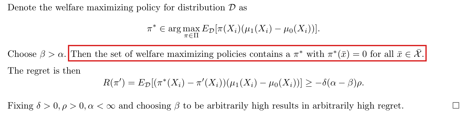
Because the rewards and are zero when nobody is treated, their expected value is , where , and is or ; the rule printed as the agent’s best response (treat only the values of with the largest positive ) need not maximize it, and on the Horse Colic data the best response to keeps 48.03% of the achievable welfare, where the printed rule keeps 5.34%.
Section 3, best responses stated after Reward Functions 1 and 2, PDF pp. 4–5; Appendix B.3, Propositions 6 and 7 and the first display of each proof, PDF pp. 15–16; proof of Proposition 2, PDF pp. 17–18; rows and of Table 1 (PDF p. 9) and Table 2 (PDF p. 27)
See also under Formal statements (Lean): P006-T1, P006-T2, P006-T3, P006-T18, P006-T26
As printed
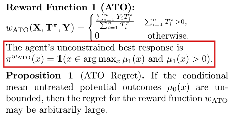
Section 3, PDF p. 4:
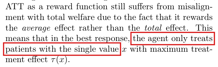
“The agent’s unconstrained best response is .”
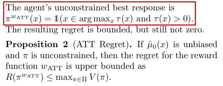
Section 3, PDF pp. 4–5:
“The agent’s unconstrained best response is . … This means that in the best response, the agent only treats patients with the single value with maximum treatment effect .”
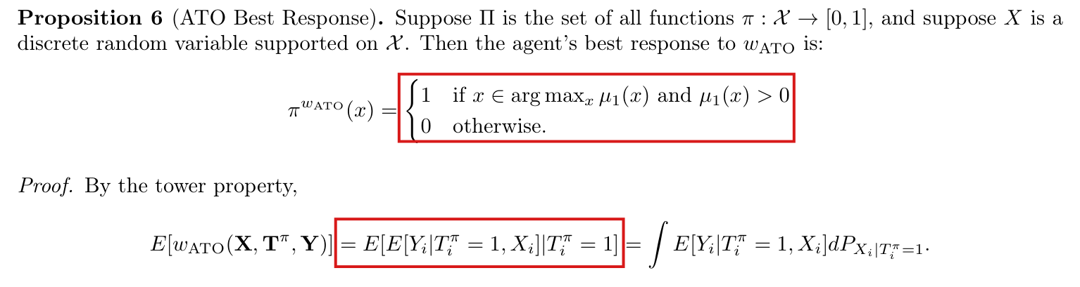
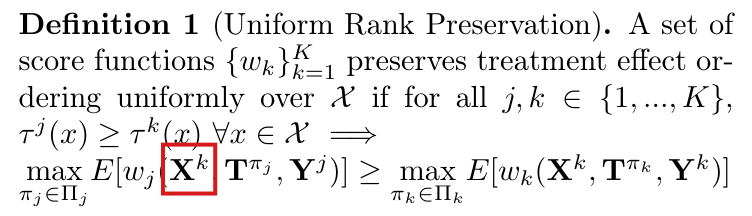
Appendix B.3, PDF p. 15: Proposition 6 (ATO Best Response). Suppose is the set of all functions , and suppose is a discrete random variable supported on . Then the agent’s best response to is:
Proof. By the tower property,
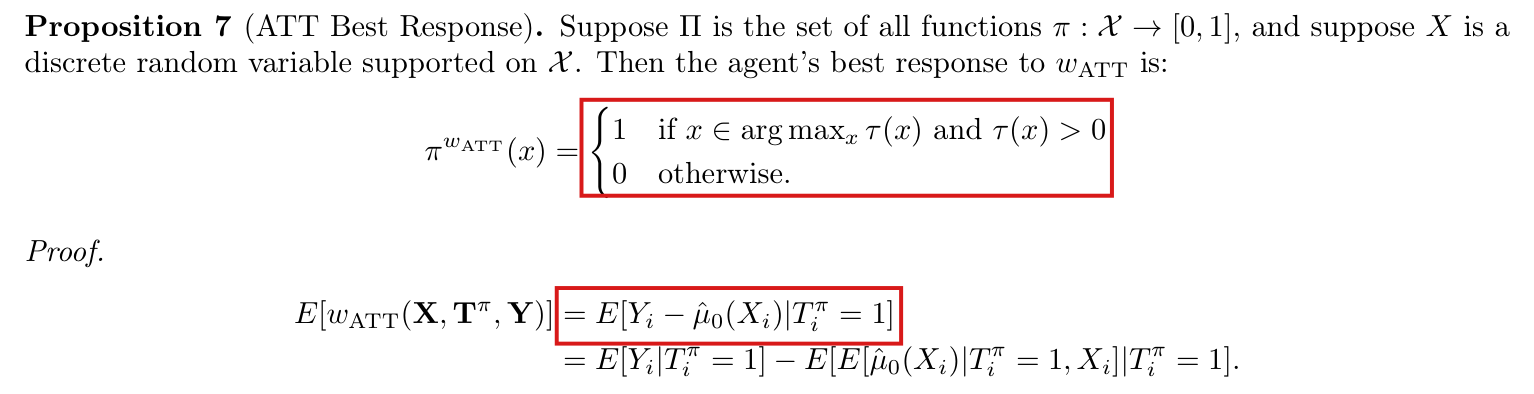
Appendix B.3, PDF p. 16: Proposition 7 (ATT Best Response). Suppose is the set of all functions , and suppose is a discrete random variable supported on . Then the agent’s best response to is:
Proof.
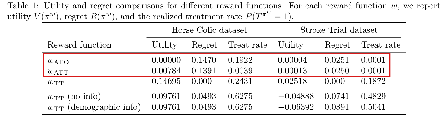
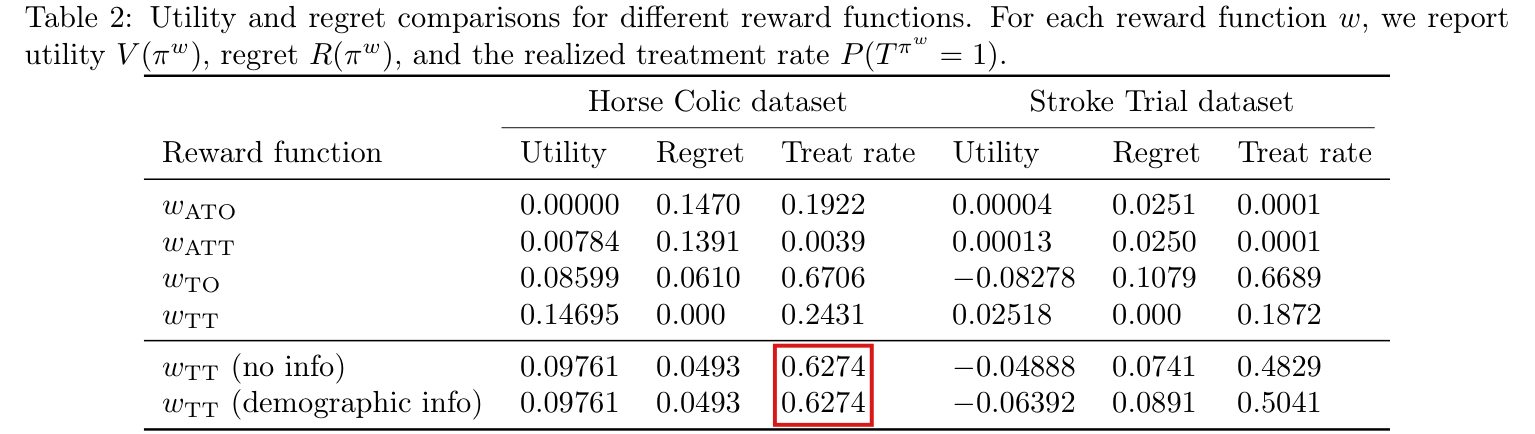
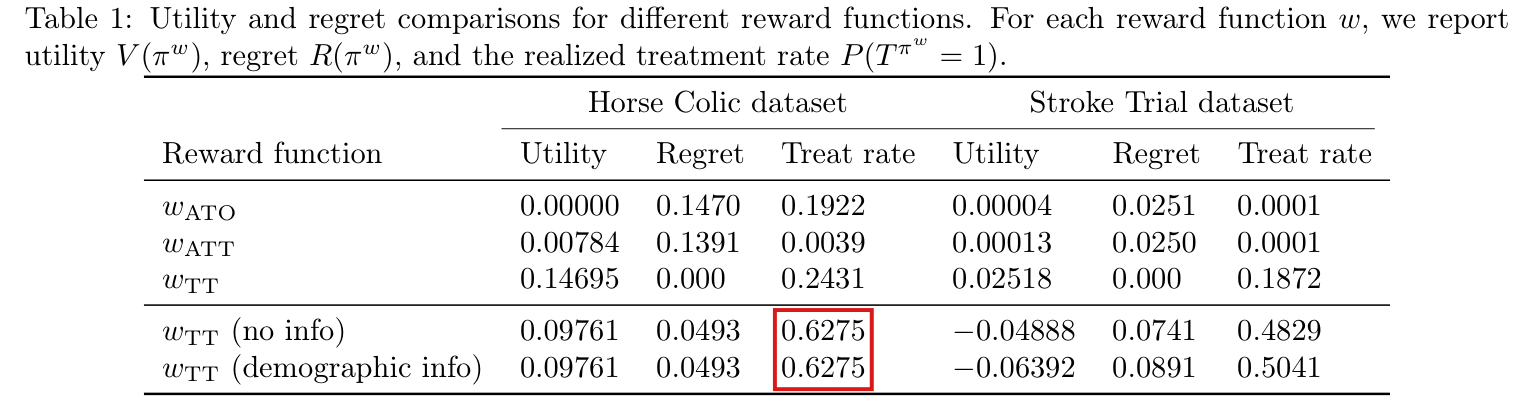
Table 1, PDF p. 9: “For each reward function , we report utility , regret , and the realized treatment rate .” The rows and are the same in Table 2, PDF p. 27.
| Reward function | Utility | Regret | Treat rate | Utility | Regret | Treat rate |
|---|---|---|---|---|---|---|
| 0.00000 | 0.1470 | 0.1922 | 0.00004 | 0.0251 | 0.0001 | |
| 0.00784 | 0.1391 | 0.0039 | 0.00013 | 0.0250 | 0.0001 |
The problem
Reward Functions 1 and 2 are averages over the treated units in a sample of units, and each is defined to be when no unit is treated. Section 2 and Appendix B.1 define the agent’s best response as the policy that maximizes the expected reward , with no conditioning. The first equality in the proof of Proposition 6, and the first in the proof of Proposition 7, replace this expectation by the mean among the treated units. That mean is the expected reward given that at least one unit is treated. The expected reward has the further factor , the probability that at least one unit is treated, where is the probability that a given unit is treated. This factor depends on the policy and increases with : a policy that treats more units is left less often with the reward . The printed rule maximizes the mean among the treated units and does not account for this factor. It therefore need not maximize the expected reward.
Section 3 states the same rule for both rewards and adds that under the agent “only treats patients with the single value with maximum treatment effect”. The proof of Proposition 2 substitutes the printed rule for the best response. The rows and of Tables 1 and 2 are computed for the printed rule: the replication files treat the units whose fitted , or fitted , equals the largest value in the sample. The captions of the tables present these rows as the utility, the regret and the treatment rate of the best response .
A recalculation from the replication files shows that the printed rule is the best response for one of the four rows, on the Horse Colic data, where 49 cases share the largest fitted . For the other three rows the best response treats more units than the printed rule. I call the largest welfare of any policy on the fitted data the achievable welfare; it is the utility in the row . For on the Horse Colic data, the best response treats nine cases where the printed rule treats one, and it keeps 48.03% of the achievable welfare where the printed rule keeps 5.34%. The printed row therefore understates the welfare under this reward on these data by a factor of about nine. On the Stroke Trial data the best responses keep 1.45% and 2.50% of the achievable welfare, and the printed rows still show correctly that welfare is low under both rewards.
The printed rule does maximize a different objective, the mean among the treated units in the population, when the maximum of or is positive and is attained with positive probability. For a fixed policy with , the expected reward tends to that mean as . The paper states neither qualification.
Evidence an exact counterexample
The evidence is a derivation of the expected reward, an exact counterexample, and a recalculation of the two rows of the tables from the replication files.
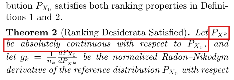
Let the units be independent and identically distributed with integrable potential outcomes, and let the treatment indicators be drawn independently given the covariates. For , suppose that is integrable and . I write for and for , and set , and . Each unit is treated with probability . By independence, I have . Let be a treatment vector of positive probability such that at least one unit is treated. Given , the term of each treated unit in the numerator of the reward (, or ) has mean . The reward is the average of these terms, so its conditional mean is also . The reward is when . Summing over , I obtain
and for . Note that the first display in each printed proof keeps only .
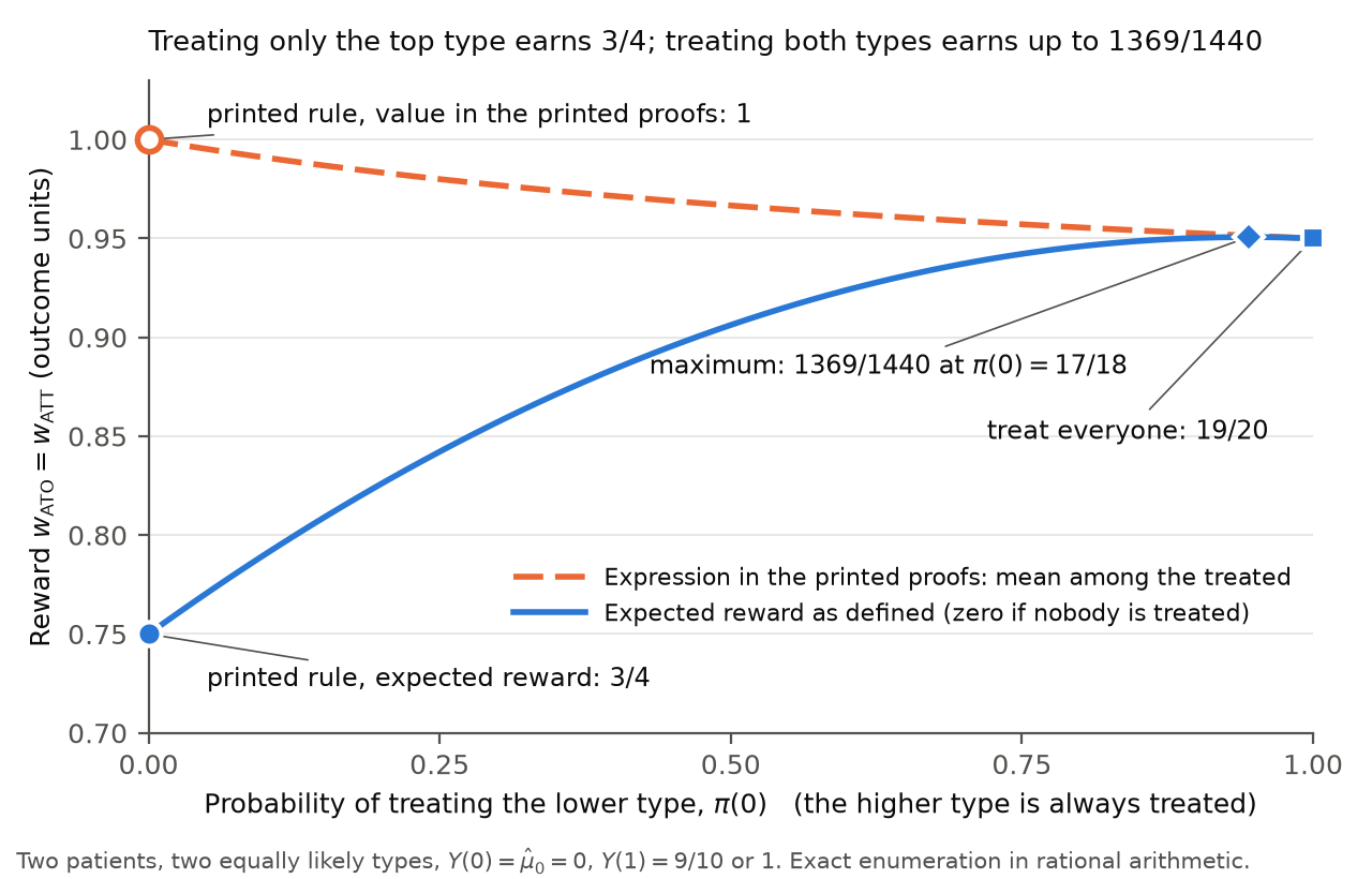
For the counterexample, I take and two equally likely types , with and , and with for type and for type . Then , the two rewards are equal, and has a unique maximum, which is positive, at . The printed rule treats type only.
| Types | Treated under the printed rule | Reward, printed rule | Reward, everyone treated |
|---|---|---|---|
| nobody | |||
| unit 2 | |||
| unit 1 | |||
| both units | |||
| Expected reward |
The policy that treats everyone has expected reward , which exceeds the expected reward of the printed rule by . For the printed rule, the right side of the first display of the printed proofs equals , and the left side equals .
Neither of these two policies is the best response. With and , the formula above gives , and
for , with equality only at and . The best response treats type with probability and type with probability , and it has expected reward .
On a finite support, the best response is found as follows. In the notation of the corrected statement below, let be the largest expected reward among the policies with , and let , so that for . On the segment , I have with , and a direct computation gives
for . The function is nonnegative and nondecreasing, and at the slope of falls from to . These two facts imply that is nonincreasing on . A value of at which changes sign from positive to negative then maximizes over . Let and , and, if , let be the largest value of below . The printed rule is the policy of this form with . On , I have , which increases with , and for the right derivative of at equals
For , the printed rule is therefore a best response if and only if . If , treating everyone is a best response.
In the replication files, both notebooks compute the row from the indicator that the fitted of a unit equals the largest fitted in the sample, and the row from the indicator that its fitted equals the largest such difference. For the recalculation, I computed the best responses to the rewards as defined on the same fitted values. The population is the empirical distribution of the cases that the notebook analyzes, with the fitted and of the notebook. There are 255 cases for the Horse Colic data and 7264 patients for the Stroke Trial data. The units are independent draws from this distribution, with equal to the number of cases, and is the set of all functions from the covariate values to . For each data set and each reward, I located the change in sign of and checked the signs on either side in exact rational arithmetic.
| Data and reward | Row | Utility | Regret | Treat rate | Expected units treated | Welfare kept (%) |
|---|---|---|---|---|---|---|
| Horse Colic, | as printed | 0.00000 | 0.1470 | 0.1922 | 49 | 0.00 |
| best response | 0.00000 | 0.1470 | 0.1922 | 49 | 0.00 | |
| Horse Colic, | as printed | 0.00784 | 0.1391 | 0.0039 | 1 | 5.34 |
| best response | 0.07058 | 0.0764 | 0.0353 | 9 | 48.03 | |
| Stroke Trial, | as printed | 0.00004 | 0.0251 | 0.0001 | 1 | 0.16 |
| best response | 0.00036 | 0.0248 | 0.0007 | 4.845 | 1.45 | |
| Stroke Trial, | as printed | 0.00013 | 0.0250 | 0.0001 | 1 | 0.52 |
| best response | 0.00063 | 0.0246 | 0.0007 | 5 | 2.50 |
On the Horse Colic data, 49 cases have a fitted equal to in the double-precision arithmetic of the notebook. The printed rule treats these 49 cases, and the best response to treats the same cases. The nine largest values of the fitted lie between and , and the tenth is . The printed rule treats the one case with the largest value, and the best response to treats the nine. The welfare of this best response is , its regret is , and it treats 3.53% of the cases. For , the expected reward is under the printed rule and under the best response. On the Stroke Trial data, the best response to treats four patients with probability and a fifth with probability , and the best response to treats five patients. The printed rule treats one patient under each reward. The condition holds for on the Horse Colic data and fails for the other three rows.
The paper gives for the Horse Colic data, and the notebook analyzes the 255 cases that remain after its exclusions. With and the same 255 cases, I find that the best responses, the welfare, the regret and the treatment rate are the same.
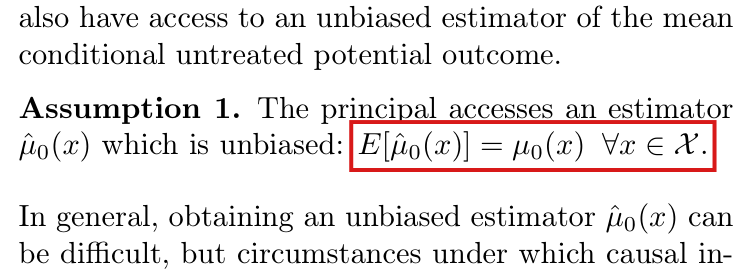
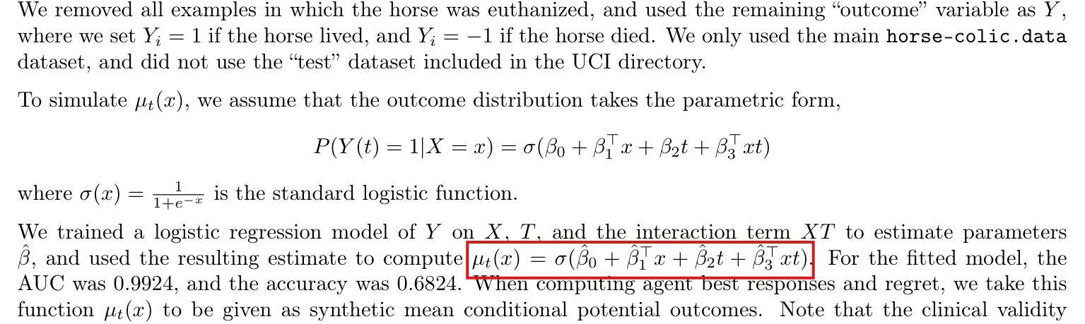
The notebook for the Stroke Trial data fits a linear model by least squares. I fitted it again from the data, and the coefficients agree with those printed in the stored output of the notebook to within . For the Horse Colic data I did not fit the logistic model again. I reconstructed the fitted values from the coefficients, which the stored output of the notebook gives to eight decimal places. The intercept is not printed, and I recovered it from the group means in the stored output. Bounds for the rounding of these numbers were carried through the calculation. For every set of fitted values within the bounds, the best response to treats the same nine cases, and it keeps between 48.0296% and 48.0297% of the achievable welfare. The tie among the 49 cases is an effect of rounding in double precision. With the logistic function evaluated to 90 decimal places, the best response to for treats 41 cases, and its welfare is still to fifteen decimal places. The best response to does not change.
What survives
The definitions of the two rewards stand, and so does the bound of Proposition 2, , with the proof given below. The conclusion of Proposition 1 also stands. With , , and , the unique best response to as defined treats type only, and with and its regret is , which is unbounded in ; for every best response has this regret. Under the same conditional unbiasedness condition, Proposition 3 does not depend on the error, because involves no division by the number of treated units. The ranking and information-asymmetry results and their rows in the tables use total-effect rewards and do not depend on it either. These are statements about dependence on this error, not a confirmation of those results.
What changes is the description of the agent under the two average rewards and the reading of the rows and of Tables 1 and 2. The agent need not treat only the best type. The printed rows summarize the printed rule, subject to the rounding corrections in P006-E018. They are the rows of the best response only for on the Horse Colic data. The statement of Section 6 that the utility for is close to zero for both datasets stands. On the Stroke Trial data both rewards still lose almost all of the achievable welfare: the best responses keep 1.45% and 2.50% of it and treat about five of the 7264 patients. On the Horse Colic data the best response to still has positive regret, but it keeps 48.03% of the achievable welfare, with welfare , regret and 3.53% of the cases treated. The printed row, with utility and regret , corresponds to 5.34%.
Corrected
Propositions 6 and 7. Suppose that , the units are independent and identically distributed with integrable potential outcomes, and the treatment indicators are drawn independently given the covariates. For , suppose also that, for every admissible policy, is integrable and , as holds for a pointwise unbiased estimator computed from independent auxiliary data with policies fixed independently of the estimator (this condition is the subject of P006-E002). Let for and for , and for a policy write and . Then
and a best response, when one exists, is a policy in that maximizes this expression. It need not treat only the values of that maximize .
Suppose in addition that is the set of all functions and that takes finitely many values, with probabilities and with the values of ordered as . Set and , with , and , which equals for . Among the policies with , the largest value of is . It is attained by the policy that treats the first values, treats the th value with probability , and treats no other value. A best response is a policy of this form with chosen to maximize over .
Let and , and suppose that . The rule that treats exactly the values of with is a best response if and only if every value of with satisfies
This condition holds when for every such , and for it holds only then. If , the policy that treats nobody is a best response.
The printed rule maximizes the mean among the treated units, , when the maximum of is positive and is attained with positive probability. It can be kept as a best-response rule for that explicitly stated alternative objective.
Section 3. The two sentences beginning “The agent’s unconstrained best response is” are replaced by the statement above, and the sentence that the agent “only treats patients with the single value with maximum treatment effect ” is withdrawn.
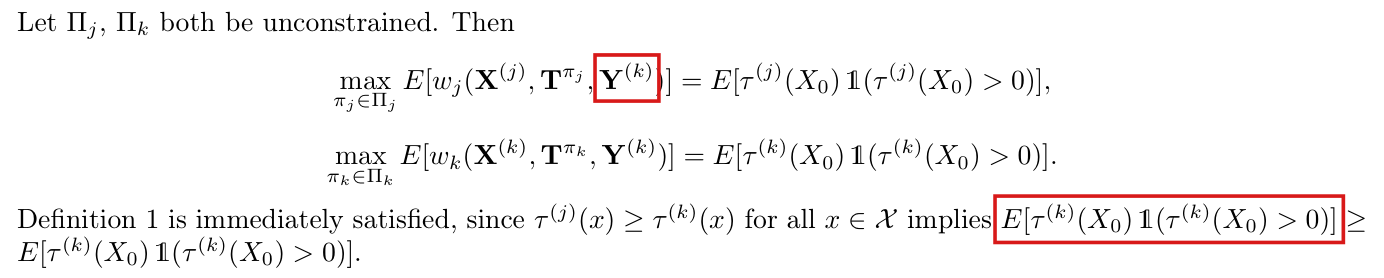
Proposition 2 (bound unchanged). Proof. Suppose the conditions stated above for . For every policy, , so with . The policy belongs to and has expected reward , so a best response has expected reward at least and therefore . Hence .
Tables 1 and 2. The two rows are computed for the best responses to the rewards as defined, using the fitted values in the double-precision arithmetic of the notebooks, with the units drawn independently from the empirical distribution of the analyzed cases: for the Horse Colic data, where gives the same row, and for the Stroke Trial data.
| Reward function | Utility | Regret | Treat rate | Utility | Regret | Treat rate |
|---|---|---|---|---|---|---|
| 0.00000 | 0.1470 | 0.1922 | 0.00036 | 0.0248 | 0.0007 | |
| 0.07058 | 0.0764 | 0.0353 | 0.00063 | 0.0246 | 0.0007 |
The rows as printed report the utility, the regret and the treatment rate of the rule that treats only the units with the largest fitted , or the largest fitted . With the corrected rows, the utility for is close to zero for both datasets, as Section 6 states. For , the best response keeps 2.50% of the achievable welfare on the Stroke Trial data and 48.03% on the Horse Colic data, where its regret is and not .























My comment and the history of this entry