LLM-generated corrections to the published research of P. M. Aronow

Conference paper P006

Corrections to: On Counterfactual Metrics for Social Welfare: Incentives, Ranking, and Information Asymmetry

Serena Wang, Stephen Bates, P. M. Aronow, and Michael I. Jordan (2024). On Counterfactual Metrics for Social Welfare: Incentives, Ranking, and Information Asymmetry. AISTATS 2024 PMLR 238:1522–1530.

arXiv
2305.14595
Audited edition
AISTATS 2024, 2024, PMLR 238:1522–1530; 28 pages in the audited file
SHA-256 of the audited file
23f6cc84d5aec6abc601f4638b7981974c8cc4221ebcc7b9839309aba043627b
Permanent address
https://pmaronow.github.io/llm-audit/works/P006/

Summary

The paper models quality metrics as a principal–agent problem: a regulator rewards a provider that chooses whom to treat. It shows that rewarding the average treated outcome can cause unbounded regret, and that rewarding the total treatment effect, with shared covariate information and an estimate unbiased at evaluated treated observations, has zero regret. 22 entries are classified as errors (1 Major, 1 Moderate, 20 Minor), and 2 are clarity notes. Four other possible errors were not confirmed, and a fifth could not be determined. The Major finding, P006-E001, is that the best responses stated for the average rewards do not hold in finite samples. In the fitted Horse Colic simulation, the recomputed best response to the average-effect reward keeps 48% of the achievable welfare, compared with 5% under the printed rule.

What was and was not checked

I checked the following by following the proofs, by recalculation from the replication files, or against the pages. They held up, subject to the corrections cited.

  • Lemma 1: V(π)=E[τ(X)π(X)]V(\pi)=E[\tau(X)\pi(X)], which is maximized over unconstrained policies by 1(τ(x)>0)\mathbf{1}(\tau(x)>0).
  • Propositions 8 and 9: E[wTO]=nE[μ1(X)π(X)]E[w_{\mathrm{TO}}]=nE[\mu_1(X)\pi(X)] and E[wTT]=nV(π)E[w_{\mathrm{TT}}]=nV(\pi) hold exactly for finite nn, the second under the corrected Assumption 1 of P006-E002. Proposition 3 follows for any feasible set.
  • Proposition 1: the first example, with regret −α(1−p)-\alpha(1-p), is correct; the second is correct after the sign correction of P006-E007.
  • Proposition 2: the bound R≤max⁡πV(π)R\le\max_\pi V(\pi) holds for the finite-sample reward by a replacement proof (P006-E001).
  • Proposition 4: the example in which a larger population reverses the ranking is valid.
  • Theorem 1: under the corrected Assumption 1 and weighted integrability conditions of P006-E002, E[wTTg]=nE[g(X)τ(X)π(X)]E[w^g_{\mathrm{TT}}]=nE[g(X)\tau(X)\pi(X)], and a strictly positive gg does not change the best response over unconstrained policies.
  • Theorem 2, with the corrections of P006-E002, P006-E005 and P006-E013. Nonnegative treatment effects are needed for Definition 2.
  • Lemma 2, Proposition 10 and Theorem 3 for an estimator from independent auxiliary data. The bound 2γmarg2\gamma_{\mathrm{marg}} was also tested on 6561 four-cell distributions in each of three policy classes and on 200000 random discrete instances, with no violation.
  • Proposition 5: the arithmetic of the construction, R=α−β/2R=\alpha-\beta/2 and γmarg=α\gamma_{\mathrm{marg}}=\alpha, for the displayed policy (P006-N006).
  • Lemma 3 and the inequalities in the proof of Theorem 5, given the positivity condition of P006-E006.
  • Stroke data: n=7264n=7264, treatment rate 0.3337, Y∈[−4,3]Y\in[-4,3], 17 categorical and 3 numerical covariates, 1360 and 5904 patients with positive and negative fitted effects. Every Stroke entry of Tables 1 and 2, the values plotted in Figure 1 and the Stroke panel of Figure 2 reproduce from the data, up to the last printed digits (P006-E018).
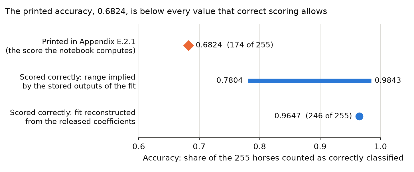
  • Horse Colic data: the preprocessing agrees with Appendix E.2.1 (20 features, 255 cases after exclusions, treatment rate 153/255=0.6153/255=0.6). The entries of Tables 1 and 2 and Figures 2 and 3 agree with the stored outputs of the released notebook, and a model reconstructed from the rounded coefficients in the released notebook reproduces the AUC 0.9924.
  • In the released calculations for Tables 1 and 2, before rounding, the regret is the wTTw_{\mathrm{TT}} utility minus the utility of the row, and the treatment rates are whole numbers of units divided by 255 and by 7264.
  • Regret amplification in the Stroke data: regret 0.0891 with demographic information against 0.0741 with none. The comparison survives the corrections of P006-E011 and P006-N003.
  • The released code implements the policies that the paper states and computes γmarg\gamma_{\mathrm{marg}} as in Appendix E.4 with the denominator corrected in P006-E015. Whether the stated responses to the average rewards are best responses is the subject of P006-E001.

The following were not checked. Neither notebook was run in its original software environment, whose versions are not recorded. The Stroke least-squares fit was reproduced with other software. I did not rerun the Horse Colic logistic fit in its original software environment. I emulated it with other solvers and reconstructed it from the stored rounded coefficients. The reconstruction reproduces the stored AUC, while other solver fits change the results because no finite maximum-likelihood estimate exists. Of the cited works I read Dranove et al. (2003) and the 2018 preprint of Kallus and Zhou. The other cited works were not read, and the paper’s quotations were not compared with their sources. The clinical validity of the fitted potential outcomes was not assessed, and the paper itself says that it cannot be verified from the data.

Two files of the Stroke database, the trial protocol and a text version of the data, were not read. The data file in CSV form was read in full. I could not find the variables that the implementation of Kallus and Zhou used, and whether the coding of the outcome score for the Stroke data reproduces theirs is not settled. These checks do not show that the paper is correct in the respects that were not examined.

Headline claims and related corrections

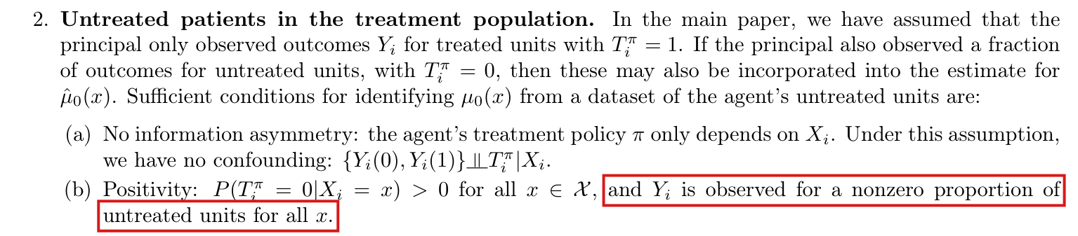
  1. Rewarding the average treated outcome (ATO), the status-quo quality metric, can produce arbitrarily large welfare regret, because it ignores untreated outcomes and rewards an average rather than a total; accounting for the untreated outcome is necessary.

    Proposition 1; Proposition 6 (ATO best response); Theorem 4 (Appendix A.2); Table 1 row wATOw_{\mathrm{ATO}}

    See P006-E001, P006-E007, P006-E003.

  2. The paper states that subtracting an unbiased estimate of the untreated outcome and rewarding the average treatment effect on the treated (ATT) bounds regret by the maximum achievable welfare. It attributes the remaining nonzero regret to the agent treating only the covariate value with the largest treatment effect.

    Proposition 2; Proposition 7 (ATT best response); Table 1 row wATTw_{\mathrm{ATT}}

    See P006-E001, P006-E002.

  3. Rewarding the total treatment effect, wTT=∑i(Yi−μ^0(Xi))Tiw_{\mathrm{TT}}=\sum_i (Y_i-\hat\mu_0(X_i))T_i, makes the best response welfare maximizing, with zero regret for any feasible policy set, given an unbiased estimate of the conditional mean untreated outcome.

    Proposition 3; Proposition 9; Lemma 1

    See P006-E002.

  4. Used directly to rank agents, wTTw_{\mathrm{TT}} violates rank preservation because population size and case mix affect scores. The weighted reward wTTgw^g_{\mathrm{TT}} retains zero regret for any positive weight gg, and reweighting to a reference covariate distribution satisfies uniform rank preservation and, for nonnegative treatment effects, relative rank preservation.

    Definitions 1-2; Proposition 4; Theorem 1; Theorem 2

    See P006-E005, P006-E013.

  5. When the agent observes covariates UU that the principal does not, an unbiased estimate of μ0(x)\mu_0(x) need not give zero regret. Regret under wTTw_{\mathrm{TT}} is at most 2γmarg2\gamma_{\mathrm{marg}}, where γmarg\gamma_{\mathrm{marg}} bounds E[∣μ0(X)−μ0(X,U)∣]E[|\mu_0(X)-\mu_0(X,U)|]; the bound is tight up to a constant, with examples having regret at least γmarg−ϵ\gamma_{\mathrm{marg}}-\epsilon.

    Assumption 2; Theorem 3; Proposition 5; Lemma 2; Proposition 10

    See P006-N006, P006-E002.

  6. If the principal estimates the untreated outcome from the agent's own untreated units, the bounded-heterogeneity condition in Assumption 4 gives regret under wTTw_{\mathrm{TT}} of at most 2γmax⁡2\gamma_{\max}.

    Section 5, 'Information asymmetry and confounding'; Appendix D.3: Assumption 4; Theorem 5; Lemma 3

    See P006-E006, P006-E014, P006-N001.

  7. On two clinical datasets with synthetic potential outcomes, Tables 1 and 2 report low welfare for the policies used with wATOw_{\mathrm{ATO}} and wATTw_{\mathrm{ATT}} relative to wTTw_{\mathrm{TT}}, which has zero reported regret. The reported achievable welfare is higher for Horse Colic than for Stroke Trial.

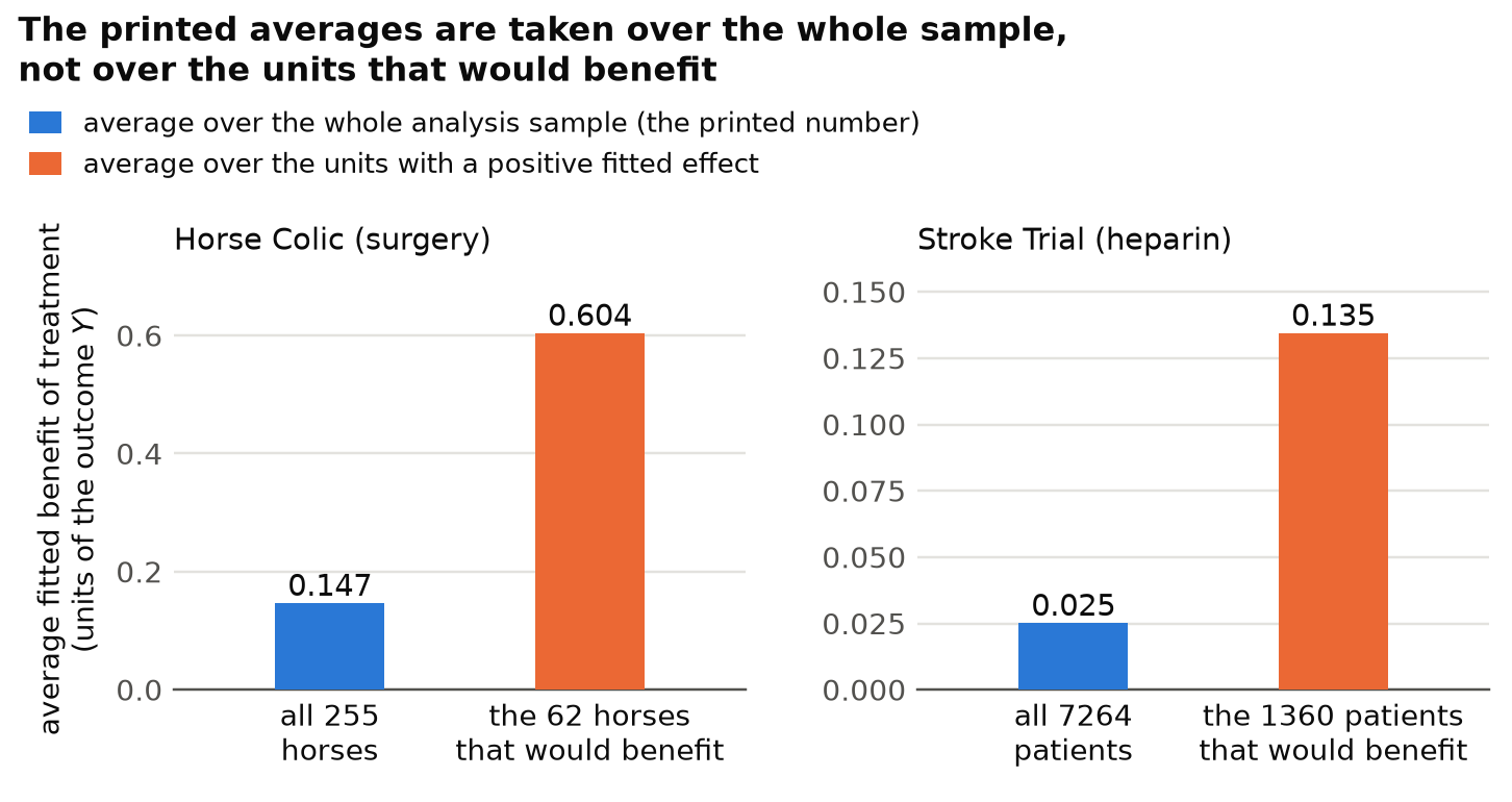
    Table 1; Table 2; Appendix E.2; Section 6 text (benefit counts and average benefit)

    See P006-E001, P006-E008, P006-E009, P006-E010, P006-E011, P006-E018, P006-N003.

  8. Under information asymmetry, conditioning the counterfactual estimate on a subset of features, such as demographics, can leave regret unchanged or increase it relative to conditioning on nothing (regret amplification); more conditioning need not be beneficial.

    Table 1 and Table 2, rows wTTw_{\mathrm{TT}} (no info) and wTTw_{\mathrm{TT}} (demographic info); Figure 2; Appendix E.5

    See P006-E011, P006-N003.

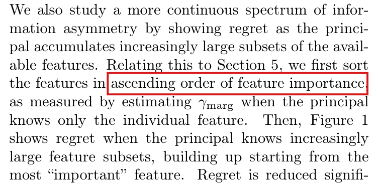
  9. In the reported experiments, regret falls as features are accumulated in increasing order of their individual γmarg\gamma_{\mathrm{marg}} and falls substantially before half the features are used. Approximate γmarg\gamma_{\mathrm{marg}} values may therefore be a useful heuristic for choosing covariates to condition on.

    Figure 1; Figure 3; Appendix E.4; Appendix E.5

    See P006-N009, P006-N004, P006-E015.

Corrections

Major (1)

A central result, method or key claim fails for a non-trivial reason, and the repair changes what the paper establishes.

Because the rewards wATOw_{\mathrm{ATO}} and wATTw_{\mathrm{ATT}} are zero when nobody is treated, their expected value is [1−(1−q)n]A/q[1-(1-q)^n]A/q, where q=E[π(X)]q=E[\pi(X)], A=E[s(X)π(X)]A=E[s(X)\pi(X)] and ss is μ1\mu_1 or τ\tau; the rule printed as the agent’s best response (treat only the values of xx with the largest positive s(x)s(x)) need not maximize it, and on the Horse Colic data the best response to wATTw_{\mathrm{ATT}} keeps 48.03% of the achievable welfare, where the printed rule keeps 5.34%.

Section 3, best responses stated after Reward Functions 1 and 2, PDF pp. 4–5; Appendix B.3, Propositions 6 and 7 and the first display of each proof, PDF pp. 15–16; proof of Proposition 2, PDF pp. 17–18; rows wATOw_{\mathrm{ATO}} and wATTw_{\mathrm{ATT}} of Table 1 (PDF p. 9) and Table 2 (PDF p. 27)

See also under Formal statements (Lean): P006-T1, P006-T2, P006-T3, P006-T18, P006-T26

My comment on this entry

As printed

Section 3, PDF p. 4:

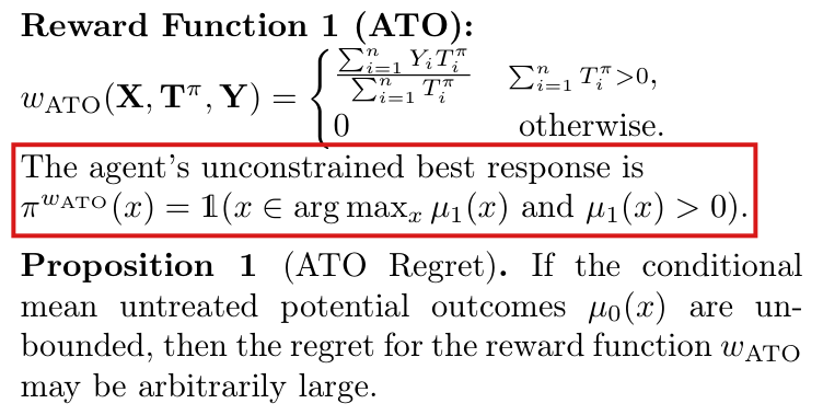
wATO(X,Tπ,Y)={∑i=1nYiTiπ∑i=1nTiπ∑i=1nTiπ>0,0otherwise.w_{\mathrm{ATO}}(\mathbf{X},\mathbf{T}^\pi,\mathbf{Y})=\begin{cases}\dfrac{\sum_{i=1}^nY_iT_i^\pi}{\sum_{i=1}^nT_i^\pi} & \sum_{i=1}^nT_i^\pi>0,\\[1ex] 0 & \text{otherwise.}\end{cases}

“The agent’s unconstrained best response is πwATO(x)=1(x∈arg⁡max⁡xμ1(x) and μ1(x)>0)\pi^{w_{\mathrm{ATO}}}(x)=\mathbb{1}(x\in\arg\max_x\mu_1(x)\text{ and }\mu_1(x)>0).”

Section 3, PDF pp. 4–5:

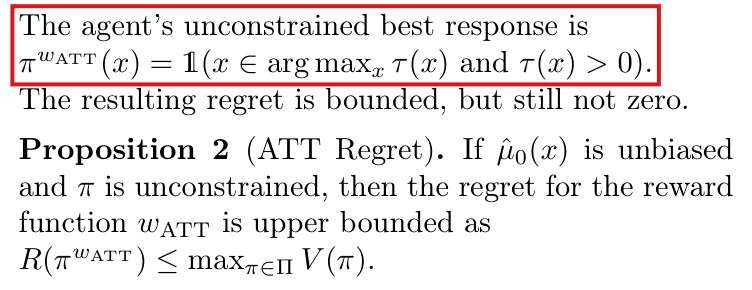
wATT(X,Tπ,Y)={∑i=1n(Yi−μ^0(Xi))Tiπ∑i=1nTiπ∑i=1nTiπ>0,0otherwise.w_{\mathrm{ATT}}(\mathbf{X},\mathbf{T}^\pi,\mathbf{Y})=\begin{cases}\dfrac{\sum_{i=1}^n(Y_i-\hat\mu_0(X_i))T_i^\pi}{\sum_{i=1}^nT_i^\pi} & \sum_{i=1}^nT_i^\pi>0,\\[1ex] 0 & \text{otherwise.}\end{cases}

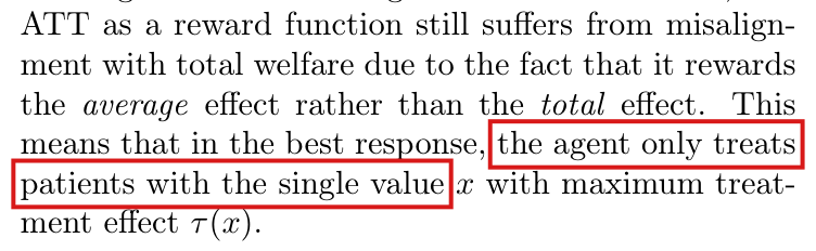
“The agent’s unconstrained best response is πwATT(x)=1(x∈arg⁡max⁡xτ(x) and τ(x)>0)\pi^{w_{\mathrm{ATT}}}(x)=\mathbb{1}(x\in\arg\max_x\tau(x)\text{ and }\tau(x)>0). … This means that in the best response, the agent only treats patients with the single value xx with maximum treatment effect τ(x)\tau(x).”

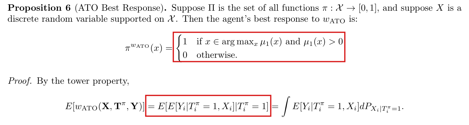
Appendix B.3, PDF p. 15: Proposition 6 (ATO Best Response). Suppose Π\Pi is the set of all functions π:X→[0,1]\pi:\mathcal{X}\to[0,1], and suppose XX is a discrete random variable supported on X\mathcal{X}. Then the agent’s best response to wATOw_{\mathrm{ATO}} is:

πwATO(x)={1if x∈arg⁡max⁡xμ1(x) and μ1(x)>00otherwise.\pi^{w_{\mathrm{ATO}}}(x)=\colorbox{#ffe58a}{$\displaystyle \begin{cases}1 & \text{if }x\in\arg\max_x\mu_1(x)\text{ and }\mu_1(x)>0\\ 0 & \text{otherwise.}\end{cases}$}

Proof. By the tower property,

E[wATO(X,Tπ,Y)]=E[E[Yi∣Tiπ=1,Xi]∣Tiπ=1]=∫E[Yi∣Tiπ=1,Xi] dPXi∣Tiπ=1.E[w_{\mathrm{ATO}}(\mathbf{X},\mathbf{T}^\pi,\mathbf{Y})]\colorbox{#ffe58a}{$\displaystyle {}=E[E[Y_i\mid T_i^\pi=1,X_i]\mid T_i^\pi=1]$}=\int E[Y_i\mid T_i^\pi=1,X_i]\,dP_{X_i\mid T_i^\pi=1}.

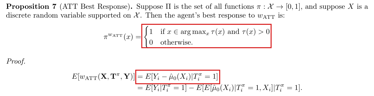
Appendix B.3, PDF p. 16: Proposition 7 (ATT Best Response). Suppose Π\Pi is the set of all functions π:X→[0,1]\pi:\mathcal{X}\to[0,1], and suppose XX is a discrete random variable supported on X\mathcal{X}. Then the agent’s best response to wATTw_{\mathrm{ATT}} is:

πwATT(x)={1if x∈arg⁡max⁡xτ(x) and τ(x)>00otherwise.\pi^{w_{\mathrm{ATT}}}(x)=\colorbox{#ffe58a}{$\displaystyle \begin{cases}1 & \text{if }x\in\arg\max_x\tau(x)\text{ and }\tau(x)>0\\ 0 & \text{otherwise.}\end{cases}$}

Proof.

E[wATT(X,Tπ,Y)]=E[Yi−μ^0(Xi)∣Tiπ=1]E[w_{\mathrm{ATT}}(\mathbf{X},\mathbf{T}^\pi,\mathbf{Y})]\colorbox{#ffe58a}{$\displaystyle {}=E[Y_i-\hat\mu_0(X_i)\mid T_i^\pi=1]$}

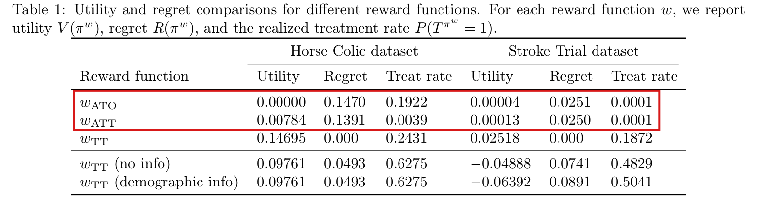
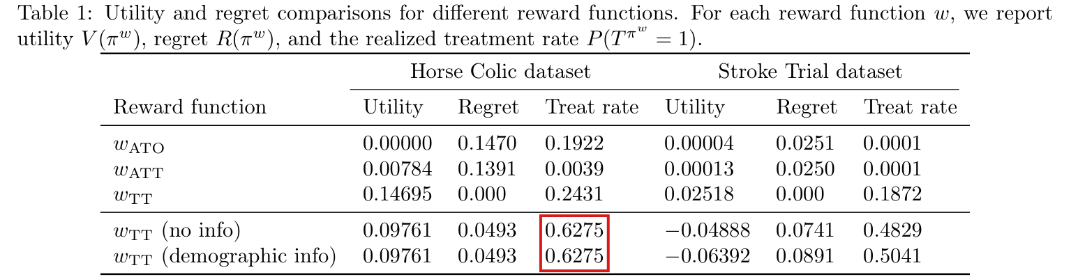
Table 1, PDF p. 9: “For each reward function ww, we report utility V(πw)V(\pi^w), regret R(πw)R(\pi^w), and the realized treatment rate P(Tπw=1)P(T^{\pi^w}=1).” The rows wATOw_{\mathrm{ATO}} and wATTw_{\mathrm{ATT}} are the same in Table 2, PDF p. 27.

Tables 1 and 2, first two rows. The first three columns of numbers are headed “Horse Colic dataset” and the last three “Stroke Trial dataset”.
Reward functionUtilityRegretTreat rateUtilityRegretTreat rate
wATOw_{\mathrm{ATO}}0.000000.14700.19220.000040.02510.0001
wATTw_{\mathrm{ATT}}0.007840.13910.00390.000130.02500.0001
The problem

Reward Functions 1 and 2 are averages over the treated units in a sample of nn units, and each is defined to be 00 when no unit is treated. Section 2 and Appendix B.1 define the agent’s best response as the policy that maximizes the expected reward E[w(X,Tπ,Y)]E[w(\mathbf{X},\mathbf{T}^\pi,\mathbf{Y})], with no conditioning. The first equality in the proof of Proposition 6, and the first in the proof of Proposition 7, replace this expectation by the mean among the treated units. That mean is the expected reward given that at least one unit is treated. The expected reward has the further factor 1−(1−q)n1-(1-q)^n, the probability that at least one unit is treated, where q=E[π(X)]q=E[\pi(X)] is the probability that a given unit is treated. This factor depends on the policy and increases with qq: a policy that treats more units is left less often with the reward 00. The printed rule maximizes the mean among the treated units and does not account for this factor. It therefore need not maximize the expected reward.

Section 3 states the same rule for both rewards and adds that under wATTw_{\mathrm{ATT}} the agent “only treats patients with the single value xx with maximum treatment effect”. The proof of Proposition 2 substitutes the printed rule for the best response. The rows wATOw_{\mathrm{ATO}} and wATTw_{\mathrm{ATT}} of Tables 1 and 2 are computed for the printed rule: the replication files treat the units whose fitted μ1\mu_1, or fitted μ1−μ0\mu_1-\mu_0, equals the largest value in the sample. The captions of the tables present these rows as the utility, the regret and the treatment rate of the best response πw\pi^w.

A recalculation from the replication files shows that the printed rule is the best response for one of the four rows, wATOw_{\mathrm{ATO}} on the Horse Colic data, where 49 cases share the largest fitted μ1\mu_1. For the other three rows the best response treats more units than the printed rule. I call the largest welfare of any policy on the fitted data the achievable welfare; it is the utility in the row wTTw_{\mathrm{TT}}. For wATTw_{\mathrm{ATT}} on the Horse Colic data, the best response treats nine cases where the printed rule treats one, and it keeps 48.03% of the achievable welfare where the printed rule keeps 5.34%. The printed row therefore understates the welfare under this reward on these data by a factor of about nine. On the Stroke Trial data the best responses keep 1.45% and 2.50% of the achievable welfare, and the printed rows still show correctly that welfare is low under both rewards.

The printed rule does maximize a different objective, the mean among the treated units in the population, when the maximum of μ1\mu_1 or τ\tau is positive and is attained with positive probability. For a fixed policy with q>0q>0, the expected reward tends to that mean as n→∞n\to\infty. The paper states neither qualification.

Evidence an exact counterexample

The evidence is a derivation of the expected reward, an exact counterexample, and a recalculation of the two rows of the tables from the replication files.

Let the units be independent and identically distributed with integrable potential outcomes, and let the treatment indicators be drawn independently given the covariates. For wATTw_{\mathrm{ATT}}, suppose that μ^0(Xi)\hat\mu_0(X_i) is integrable and E[μ^0(Xi)∣X,Tπ]=μ0(Xi)E[\hat\mu_0(X_i)\mid\mathbf{X},\mathbf{T}^\pi]=\mu_0(X_i). I write s=μ1s=\mu_1 for wATOw_{\mathrm{ATO}} and s=τs=\tau for wATTw_{\mathrm{ATT}}, and set q=E[π(X)]q=E[\pi(X)], A=E[s(X)π(X)]A=E[s(X)\pi(X)] and N=∑i=1nTiπN=\sum_{i=1}^nT_i^\pi. Each unit is treated with probability qq. By independence, I have P(N=0)=(1−q)nP(N=0)=(1-q)^n. Let t∈{0,1}nt\in\{0,1\}^n be a treatment vector of positive probability such that at least one unit is treated. Given Tπ=t\mathbf{T}^\pi=t, the term of each treated unit in the numerator of the reward (YiY_i, or Yi−μ^0(Xi)Y_i-\hat\mu_0(X_i)) has mean A/qA/q. The reward is the average of these terms, so its conditional mean is also A/qA/q. The reward is 00 when N=0N=0. Summing over tt, I obtain

E[w(X,Tπ,Y)]=[1−(1−q)n]Aqfor q>0,E[w(\mathbf{X},\mathbf{T}^\pi,\mathbf{Y})]=\bigl[1-(1-q)^n\bigr]\frac{A}{q}\qquad\text{for }q>0,

and E[w(X,Tπ,Y)]=0E[w(\mathbf{X},\mathbf{T}^\pi,\mathbf{Y})]=0 for q=0q=0. Note that the first display in each printed proof keeps only A/qA/q.

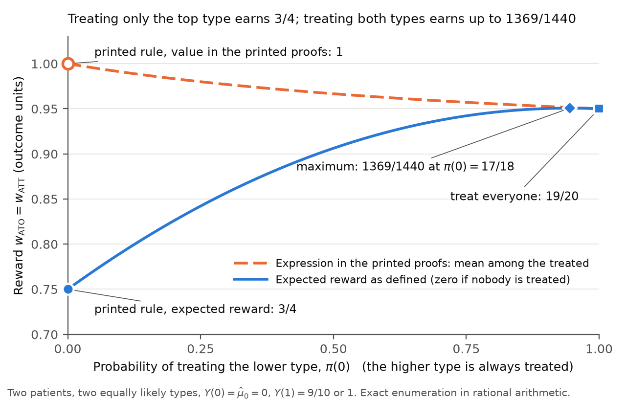
For the counterexample, I take n=2n=2 and two equally likely types x∈{0,1}x\in\{0,1\}, with Y(0)=0Y(0)=0 and μ^0=0\hat\mu_0=0, and with Y(1)=9/10Y(1)=9/10 for type 00 and Y(1)=1Y(1)=1 for type 11. Then μ1=τ\mu_1=\tau, the two rewards are equal, and μ1\mu_1 has a unique maximum, which is positive, at x=1x=1. The printed rule treats type 11 only.

The counterexample with two units. Each pair of types has probability 1/41/4.
Types (X1,X2)(X_1,X_2)Treated under the printed ruleReward, printed ruleReward, everyone treated
(0,0)(0,0)nobody009/109/10
(0,1)(0,1)unit 21119/2019/20
(1,0)(1,0)unit 11119/2019/20
(1,1)(1,1)both units1111
Expected reward3/43/419/2019/20

The policy that treats everyone has expected reward 19/2019/20, which exceeds the expected reward 3/43/4 of the printed rule by 1/51/5. For the printed rule, the right side of the first display of the printed proofs equals 11, and the left side equals 3/43/4.

Neither of these two policies is the best response. With u=π(0)u=\pi(0) and v=π(1)v=\pi(1), the formula above gives E[w]=(9u+10v)(4−u−v)/40E[w]=(9u+10v)(4-u-v)/40, and

13691440−(9u+10v)(4−u−v)40=940(u−1718)2+(1−v)(30−19u−10v)40≥0\frac{1369}{1440}-\frac{(9u+10v)(4-u-v)}{40}=\frac{9}{40}\Bigl(u-\frac{17}{18}\Bigr)^2+\frac{(1-v)(30-19u-10v)}{40}\ge0

for 0≤u,v≤10\le u,v\le1, with equality only at u=17/18u=17/18 and v=1v=1. The best response treats type 00 with probability 17/1817/18 and type 11 with probability 11, and it has expected reward 1369/14401369/1440.

On a finite support, the best response is found as follows. In the notation of the corrected statement below, let F(q)=hn(q)Amax⁡(q)F(q)=h_n(q)A_{\max}(q) be the largest expected reward among the policies with E[π(X)]=qE[\pi(X)]=q, and let g(q)=1−(1−q)ng(q)=1-(1-q)^n, so that F(q)=g(q)Amax⁡(q)/qF(q)=g(q)A_{\max}(q)/q for q>0q>0. On the segment Qj−1≤q≤QjQ_{j-1}\le q\le Q_j, I have Amax⁡(q)=aj+sjqA_{\max}(q)=a_j+s_jq with aj=∑i<jpi(si−sj)≥0a_j=\sum_{i<j}p_i(s_i-s_j)\ge0, and a direct computation gives

F′(q)=g′(q)[sj−ajHn(q)],Hn(q)=g(q)−qg′(q)q2g′(q)=1n∑l=1n−1(n−l)(1−q)−l,F'(q)=g'(q)\bigl[s_j-a_jH_n(q)\bigr],\qquad H_n(q)=\frac{g(q)-qg'(q)}{q^2g'(q)}=\frac{1}{n}\sum_{l=1}^{n-1}(n-l)(1-q)^{-l},

for 0<q<10<q<1. The function HnH_n is nonnegative and nondecreasing, and at q=Qjq=Q_j the slope of Amax⁡A_{\max} falls from sjs_j to sj+1s_{j+1}. These two facts imply that F′(q)/g′(q)F'(q)/g'(q) is nonincreasing on (0,1)(0,1). A value of qq at which F′F' changes sign from positive to negative then maximizes FF over [0,1][0,1]. Let M=s1>0M=s_1>0 and p=P(s(X)=M)p=P(s(X)=M), and, if p<1p<1, let s′s' be the largest value of ss below MM. The printed rule is the policy of this form with q=pq=p. On 0<q≤p0<q\le p, I have F(q)=Mg(q)F(q)=Mg(q), which increases with qq, and for p<1p<1 the right derivative of FF at pp equals

g(p)p[s′−M(1−rn(p))],rn(p)=pg′(p)g(p)=np(1−p)n−11−(1−p)n.\frac{g(p)}{p}\Bigl[s'-M\bigl(1-r_n(p)\bigr)\Bigr],\qquad r_n(p)=\frac{pg'(p)}{g(p)}=\frac{np(1-p)^{n-1}}{1-(1-p)^n}.

For p<1p<1, the printed rule is therefore a best response if and only if s′≤M(1−rn(p))s'\le M(1-r_n(p)). If p=1p=1, treating everyone is a best response.

In the replication files, both notebooks compute the row wATOw_{\mathrm{ATO}} from the indicator that the fitted μ1\mu_1 of a unit equals the largest fitted μ1\mu_1 in the sample, and the row wATTw_{\mathrm{ATT}} from the indicator that its fitted μ1−μ0\mu_1-\mu_0 equals the largest such difference. For the recalculation, I computed the best responses to the rewards as defined on the same fitted values. The population is the empirical distribution of the cases that the notebook analyzes, with the fitted μ0\mu_0 and μ1\mu_1 of the notebook. There are 255 cases for the Horse Colic data and 7264 patients for the Stroke Trial data. The nn units are independent draws from this distribution, with nn equal to the number of cases, and Π\Pi is the set of all functions from the covariate values to [0,1][0,1]. For each data set and each reward, I located the change in sign of F′F' and checked the signs on either side in exact rational arithmetic.

Rows wATOw_{\mathrm{ATO}} and wATTw_{\mathrm{ATT}} of Tables 1 and 2 as printed, and the same rows for the best response to the rewards as defined, rounded as in the tables. The last two columns are computed from unrounded values: the expected number of units treated, and the welfare as a percentage of the achievable welfare. In the rows as printed, these two columns are those of the printed rule in the replication files.
Data and rewardRowUtilityRegretTreat rateExpected units treatedWelfare kept (%)
Horse Colic, wATOw_{\mathrm{ATO}}as printed0.000000.14700.1922490.00
best response0.000000.14700.1922490.00
Horse Colic, wATTw_{\mathrm{ATT}}as printed0.007840.13910.003915.34
best response0.070580.07640.0353948.03
Stroke Trial, wATOw_{\mathrm{ATO}}as printed0.000040.02510.000110.16
best response0.000360.02480.00074.8451.45
Stroke Trial, wATTw_{\mathrm{ATT}}as printed0.000130.02500.000110.52
best response0.000630.02460.000752.50

On the Horse Colic data, 49 cases have a fitted μ1\mu_1 equal to 11 in the double-precision arithmetic of the notebook. The printed rule treats these 49 cases, and the best response to wATOw_{\mathrm{ATO}} treats the same cases. The nine largest values of the fitted μ1−μ0\mu_1-\mu_0 lie between 1.99941.9994 and 2.00002.0000, and the tenth is 1.90621.9062. The printed rule treats the one case with the largest value, and the best response to wATTw_{\mathrm{ATT}} treats the nine. The welfare of this best response is 0.07060.0706, its regret is 0.07640.0764, and it treats 3.53% of the cases. For n=255n=255, the expected reward is 1.26571.2657 under the printed rule and 1.99961.9996 under the best response. On the Stroke Trial data, the best response to wATOw_{\mathrm{ATO}} treats four patients with probability 11 and a fifth with probability 0.84520.8452, and the best response to wATTw_{\mathrm{ATT}} treats five patients. The printed rule treats one patient under each reward. The condition s′≤M(1−rn(p))s'\le M(1-r_n(p)) holds for wATOw_{\mathrm{ATO}} on the Horse Colic data and fails for the other three rows.

The paper gives n=300n=300 for the Horse Colic data, and the notebook analyzes the 255 cases that remain after its exclusions. With n=300n=300 and the same 255 cases, I find that the best responses, the welfare, the regret and the treatment rate are the same.

The notebook for the Stroke Trial data fits a linear model by least squares. I fitted it again from the data, and the coefficients agree with those printed in the stored output of the notebook to within 5×10−105\times10^{-10}. For the Horse Colic data I did not fit the logistic model again. I reconstructed the fitted values from the coefficients, which the stored output of the notebook gives to eight decimal places. The intercept is not printed, and I recovered it from the group means in the stored output. Bounds for the rounding of these numbers were carried through the calculation. For every set of fitted values within the bounds, the best response to wATTw_{\mathrm{ATT}} treats the same nine cases, and it keeps between 48.0296% and 48.0297% of the achievable welfare. The tie among the 49 cases is an effect of rounding in double precision. With the logistic function evaluated to 90 decimal places, the best response to wATOw_{\mathrm{ATO}} for n=255n=255 treats 41 cases, and its welfare is still 00 to fifteen decimal places. The best response to wATTw_{\mathrm{ATT}} does not change.

What survives

The definitions of the two rewards stand, and so does the bound of Proposition 2, R(πwATT)≤max⁡π∈ΠV(π)R(\pi^{w_{\mathrm{ATT}}})\le\max_{\pi\in\Pi}V(\pi), with the proof given below. The conclusion of Proposition 1 also stands. With P(X=1)=p∈(0,1)P(X=1)=p\in(0,1), μ1(0)=0\mu_1(0)=0, μ1(1)=1\mu_1(1)=1 and n≥2n\ge2, the unique best response to wATOw_{\mathrm{ATO}} as defined treats type 11 only, and with μ0(0)=0\mu_0(0)=0 and μ0(1)=B>1\mu_0(1)=B>1 its regret is p(B−1)p(B-1), which is unbounded in BB; for n=1n=1 every best response has this regret. Under the same conditional unbiasedness condition, Proposition 3 does not depend on the error, because E[wTT]=nV(π)E[w_{\mathrm{TT}}]=nV(\pi) involves no division by the number of treated units. The ranking and information-asymmetry results and their rows in the tables use total-effect rewards and do not depend on it either. These are statements about dependence on this error, not a confirmation of those results.

What changes is the description of the agent under the two average rewards and the reading of the rows wATOw_{\mathrm{ATO}} and wATTw_{\mathrm{ATT}} of Tables 1 and 2. The agent need not treat only the best type. The printed rows summarize the printed rule, subject to the rounding corrections in P006-E018. They are the rows of the best response only for wATOw_{\mathrm{ATO}} on the Horse Colic data. The statement of Section 6 that the utility for wATOw_{\mathrm{ATO}} is close to zero for both datasets stands. On the Stroke Trial data both rewards still lose almost all of the achievable welfare: the best responses keep 1.45% and 2.50% of it and treat about five of the 7264 patients. On the Horse Colic data the best response to wATTw_{\mathrm{ATT}} still has positive regret, but it keeps 48.03% of the achievable welfare, with welfare 0.07060.0706, regret 0.07640.0764 and 3.53% of the cases treated. The printed row, with utility 0.007840.00784 and regret 0.13910.1391, corresponds to 5.34%.

Corrected

Propositions 6 and 7. Suppose that n≥1\colorbox{#ffe58a}{$n\ge1$}, the units are independent and identically distributed with integrable potential outcomes, and the treatment indicators are drawn independently given the covariates. For wATTw_{\mathrm{ATT}}, suppose also that, for every admissible policy, μ^0(Xi)\hat\mu_0(X_i) is integrable and E[μ^0(Xi)∣X,Tπ]=μ0(Xi)E[\hat\mu_0(X_i)\mid\mathbf{X},\mathbf{T}^\pi]=\mu_0(X_i), as holds for a pointwise unbiased estimator computed from independent auxiliary data with policies fixed independently of the estimator (this condition is the subject of P006-E002). Let s=μ1s=\mu_1 for wATOw_{\mathrm{ATO}} and s=τs=\tau for wATTw_{\mathrm{ATT}}, and for a policy π\pi write q=E[π(X)]q=E[\pi(X)] and A=E[s(X)π(X)]A=E[s(X)\pi(X)]. Then

E[w(X,Tπ,Y)]={[1−(1−q)n] Aqq>0,0q=0,E[w(\mathbf{X},\mathbf{T}^\pi,\mathbf{Y})]=\begin{cases}{}\colorbox{#ffe58a}{$\displaystyle \bigl[1-(1-q)^n\bigr]$}\,\dfrac{A}{q} & q>0,\\[1ex] 0 & q=0,\end{cases}

and a best response, when one exists, is a policy in Π\Pi that maximizes this expression. It need not treat only the values of xx that maximize ss.

Suppose in addition that Π\Pi is the set of all functions π:X→[0,1]\pi:\mathcal{X}\to[0,1] and that XX takes finitely many values, with probabilities p1,…,pK>0p_1,\dots,p_K>0 and with the values of ss ordered as s1≥⋯≥sKs_1\ge\dots\ge s_K. Set Qj=p1+⋯+pjQ_j=p_1+\dots+p_j and Bj=p1s1+⋯+pjsjB_j=p_1s_1+\dots+p_js_j, with Q0=B0=0Q_0=B_0=0, and hn(q)=∑k=0n−1(1−q)kh_n(q)=\sum_{k=0}^{n-1}(1-q)^k, which equals [1−(1−q)n]/q[1-(1-q)^n]/q for q>0q>0. Among the policies with E[π(X)]=q∈[Qj−1,Qj]E[\pi(X)]=q\in[Q_{j-1},Q_j], the largest value of AA is Amax⁡(q)=Bj−1+sj(q−Qj−1)A_{\max}(q)=B_{j-1}+s_j(q-Q_{j-1}). It is attained by the policy that treats the first j−1j-1 values, treats the jjth value with probability (q−Qj−1)/pj(q-Q_{j-1})/p_j, and treats no other value. A best response is a policy of this form with qq chosen to maximize hn(q)Amax⁡(q)h_n(q)A_{\max}(q) over 0≤q≤10\le q\le1.

Let M=s1M=s_1 and p=P(s(X)=M)p=P(s(X)=M), and suppose that M>0M>0. The rule that treats exactly the values of xx with s(x)=Ms(x)=M is a best response if and only if every value of xx with s(x)<Ms(x)<M satisfies

s(x)≤M[1−np(1−p)n−11−(1−p)n].s(x)\le M\Bigl[1-\frac{np(1-p)^{n-1}}{1-(1-p)^n}\Bigr].

This condition holds when s(x)≤0s(x)\le0 for every such xx, and for n=1n=1 it holds only then. If M≤0M\le0, the policy that treats nobody is a best response.

The printed rule maximizes the mean among the treated units, A/qA/q, when the maximum of ss is positive and is attained with positive probability. It can be kept as a best-response rule for that explicitly stated alternative objective.

Section 3. The two sentences beginning “The agent’s unconstrained best response is” are replaced by the statement above, and the sentence that the agent “only treats patients with the single value xx with maximum treatment effect τ(x)\tau(x)” is withdrawn.

Proposition 2 (bound unchanged). Proof. Suppose the conditions stated above for wATTw_{\mathrm{ATT}}. For every policy, V(π)=E[π(X)τ(X)]=AV(\pi)=E[\pi(X)\tau(X)]=A, so E[wATT]=hn(q)V(π)E[w_{\mathrm{ATT}}]=h_n(q)V(\pi) with hn(q)>0h_n(q)>0. The policy π≡0\pi\equiv0 belongs to Π\Pi and has expected reward 00, so a best response πwATT\pi^{w_{\mathrm{ATT}}} has expected reward at least 00 and therefore V(πwATT)≥0V(\pi^{w_{\mathrm{ATT}}})\ge0. Hence R(πwATT)=max⁡π∈ΠV(π)−V(πwATT)≤max⁡π∈ΠV(π)R(\pi^{w_{\mathrm{ATT}}})=\max_{\pi\in\Pi}V(\pi)-V(\pi^{w_{\mathrm{ATT}}})\le\max_{\pi\in\Pi}V(\pi).

Tables 1 and 2. The two rows are computed for the best responses to the rewards as defined, using the fitted values in the double-precision arithmetic of the notebooks, with the nn units drawn independently from the empirical distribution of the analyzed cases: n=255n=255 for the Horse Colic data, where n=300n=300 gives the same row, and n=7264n=7264 for the Stroke Trial data.

Tables 1 and 2, first two rows, for the best responses to the rewards as defined. The first three columns of numbers are for the Horse Colic dataset and the last three for the Stroke Trial dataset.
Reward functionUtilityRegretTreat rateUtilityRegretTreat rate
wATOw_{\mathrm{ATO}}0.000000.14700.19220.000360.02480.0007
wATTw_{\mathrm{ATT}}0.070580.07640.03530.000630.02460.0007

The rows as printed report the utility, the regret and the treatment rate of the rule that treats only the units with the largest fitted μ1\mu_1, or the largest fitted μ1−μ0\mu_1-\mu_0. With the corrected rows, the utility for wATOw_{\mathrm{ATO}} is close to zero for both datasets, as Section 6 states. For wATTw_{\mathrm{ATT}}, the best response keeps 2.50% of the achievable welfare on the Stroke Trial data and 48.03% on the Horse Colic data, where its regret is 0.07640.0764 and not 0.13910.1391.

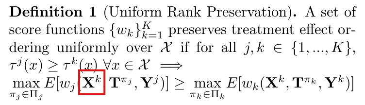
Crop of Proposition 6 (ATO Best Response), its displayed rule, and the first display of the proof. One red box marks the two cases of the rule: 1 if x is in the arg max of mu 1 and mu 1 of x is positive, 0 otherwise. A second red box marks the middle expression of the proof's display, 'equals E of E of Y i given T i equals 1 and X i, given T i equals 1', which follows 'E of w ATO'.
Appendix B.3, PDF p. 15: Proposition 6 and the first display of its proof. The upper mark is the printed best response to wATOw_{\mathrm{ATO}}. The lower mark is the equality that replaces the expected reward by the mean among the treated units.
Crop of Proposition 7 (ATT Best Response), its displayed rule, and the first two lines of the proof. One red box marks the two cases of the rule: 1 if x is in the arg max of tau and tau of x is positive, 0 otherwise. A second red box marks the right side of the first line of the proof, 'equals E of Y i minus mu hat 0 of X i, given T i equals 1'.
Appendix B.3, PDF p. 16: Proposition 7 and the first display of its proof. The upper mark is the printed best response to wATTw_{\mathrm{ATT}}, and the lower mark is the corresponding equality.
Crop of the left column showing 'Reward Function 1 (ATO)', whose definition has two cases, the average of the treated outcomes when at least one unit is treated and 0 otherwise, followed by the statement of Proposition 1. A red box marks the sentence 'The agent's unconstrained best response is pi of x equals the indicator that x is in the arg max of mu 1 and mu 1 of x is positive.'
Section 3, PDF p. 4, left column: Reward Function 1 and the best response stated after it. The second case of the definition sets the reward to 00 when nobody is treated. The marked sentence gives the rule.
Crop of the first seven lines of the left column. A red box marks the sentence 'The agent's unconstrained best response is pi of x equals the indicator that x is in the arg max of tau and tau of x is positive.' Below it are the sentence 'The resulting regret is bounded, but still not zero.' and the statement of Proposition 2 (ATT Regret).
Section 3, PDF p. 5, left column, top: the best response stated for Reward Function 2 (marked), followed by Proposition 2.
Crop of six lines of the left column. Two red boxes mark the words 'the agent only treats patients with the single value' in the sentence 'This means that in the best response, the agent only treats patients with the single value x with maximum treatment effect tau of x.'
Section 3, PDF p. 5, left column: the sentence that describes the best response to wATTw_{\mathrm{ATT}} in words.
Crop of Table 1 with its caption: Utility and regret comparisons for different reward functions. For each reward function w, we report utility V of pi w, regret R of pi w, and the realized treatment rate. The table has the columns Utility, Regret and Treat rate for the Horse Colic dataset and for the Stroke Trial dataset, and five rows. A red box surrounds the first two rows: w ATO with 0.00000, 0.1470, 0.1922 and 0.00004, 0.0251, 0.0001; w ATT with 0.00784, 0.1391, 0.0039 and 0.00013, 0.0250, 0.0001. Below the box are the rows w TT, with 0.14695, 0.000, 0.2431 and 0.02518, 0.000, 0.1872, w TT (no info) and w TT (demographic info).
Table 1, PDF p. 9, with its caption. The mark surrounds the rows wATOw_{\mathrm{ATO}} and wATTw_{\mathrm{ATT}}, which the caption describes as the utility, the regret and the treatment rate of the best response πw\pi^w.
Line chart. The horizontal axis is the probability of treating the lower type, from 0 to 1, and the vertical axis is the reward, with labelled ticks from 0.70 to 1.00. A solid blue curve, the expected reward as defined, rises from 3/4 at 0 to a maximum of 1369/1440 at 17/18 and ends at 19/20 at 1. A dashed orange curve, the mean among the treated units, falls from 1 at 0 to 19/20 at 1. At 0 an open orange circle is labelled 'printed rule, value in the printed proofs: 1' and a filled blue circle is labelled 'printed rule, expected reward: 3/4'. A blue diamond marks the maximum and a blue square marks 'treat everyone: 19/20'.
The counterexample with two units: the reward as a function of the probability π(0)\pi(0) of treating type 00, when type 11 is always treated. The solid curve is the expected reward as defined. The dashed curve is the mean among the treated units, which is the expression in the printed proofs. The printed rule is the point π(0)=0\pi(0)=0, where the printed proofs give 11 and the expected reward is 3/43/4; the maximum of the expected reward, 1369/14401369/1440, is at π(0)=17/18\pi(0)=17/18.
My comment and the history of this entry

I agree.

  1. Classification before my review (the classification when the audit was first completed, before I reviewed it): Major error.
  2. I commented.
  3. Independent evaluation. My comment agrees with the entry; no change.

Moderate (1)

A real substantive error with limited reach.

Assumption 1, unbiasedness of μ^0(x)\hat\mu_0(x) at each fixed xx, does not imply the unbiasedness at the agent’s treated observations that the proofs use; conditional unbiasedness at those observations repairs the estimator substitution in the zero-regret, ranking and 2γmarg2\gamma_{\mathrm{marg}} proofs, and is supplied by a pointwise unbiased estimator from independent auxiliary data.

Assumption 1, PDF p. 4, right column; proofs of Proposition 7 (PDF p. 16), Proposition 9 (PDF p. 17) and Theorem 3 (PDF p. 22)

See also under Formal statements (Lean): P006-T4, P006-T5, P006-T6, P006-T7, P006-T8, P006-T27

Revised: see the history of this entry.

As printed

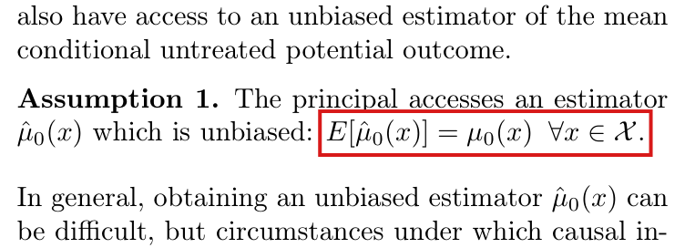
Assumption 1 (PDF p. 4). The principal accesses an estimator μ^0(x)\hat\mu_0(x) which is unbiased:

E[μ^0(x)]=μ0(x)  ∀x∈X.\colorbox{#ffe58a}{$\displaystyle E[\hat\mu_0(x)] = \mu_0(x)\ \ \forall x\in\mathcal X$}.

Proof of Proposition 7 (PDF p. 16). Since E[μ^0(x)]=μ0(x)E[\hat\mu_0(x)] = \mu_0(x) for all x∈Xx\in\mathcal X, we have

E[μ^0(Xi)∣Tiπ=1,Xi]=μ0(Xi).\colorbox{#ffe58a}{$\displaystyle E[\hat\mu_0(X_i)\mid T_i^\pi=1,X_i] = \mu_0(X_i)$}.

Thus, …

Proof of Proposition 9 (PDF p. 17). Since E[μ^0(x)]=μ0(x)E[\hat\mu_0(x)] = \mu_0(x) for all x∈Xx\in\mathcal X, we have

E[μ^0(Xi)∣Tiπ=1]=E[μ0(Xi)∣Tiπ=1].\colorbox{#ffe58a}{$\displaystyle E[\hat\mu_0(X_i)\mid T_i^\pi=1] = E[\mu_0(X_i)\mid T_i^\pi=1]$}.

Thus, …

Proof of Theorem 3 (PDF p. 22). By the tower property,

E[π(X,U)μ^0(X)]=E[E[μ^0(Xi)π(Xi,Ui)∣Xi,Ui]]=E[π(Xi,Ui)E[μ^0(Xi)∣Xi,Ui]]=E[π(Xi,Ui)μ0(Xi)].\begin{aligned} E[\pi(X,U)\hat\mu_0(X)] &= E[E[\hat\mu_0(X_i)\pi(X_i,U_i)\mid X_i,U_i]] \\ &= E[\pi(X_i,U_i)E[\hat\mu_0(X_i)\mid X_i,U_i]] \\ &= \colorbox{#ffe58a}{$\displaystyle E[\pi(X_i,U_i)\mu_0(X_i)]$}. \end{aligned}
The problem

Assumption 1 fixes the mean of the random function μ^0\hat\mu_0 at each fixed argument xx. The proofs use the mean of μ^0\hat\mu_0 at the agent’s own treated observations, that is, of μ^0(Xi)\hat\mu_0(X_i) given Tiπ=1T_i^\pi=1. The first does not imply the second when the estimator depends on the sample on which the agent is scored. In that case μ^0(Xi)\hat\mu_0(X_i) can be biased for μ0(Xi)\mu_0(X_i) although μ^0(x)\hat\mu_0(x) is unbiased for every fixed xx, so the three highlighted steps need not hold. If Assumption 1 is the only condition on the estimator, then the conclusions drawn from these steps fail as well: the best responses of Propositions 7 and 9, the bound of Proposition 2, the zero regret of Proposition 3 and Theorem 1, the ranking property of Theorem 2, and the bound 2γmarg2\gamma_{\mathrm{marg}} of Theorem 3.

The paper does not exclude such estimators. The auxiliary data on PDF p. 4 are introduced as “a concrete example”, and Appendix A.1, item 2, proposes to add the agent’s own untreated units to the estimate of μ0\mu_0. Assumption 1 is a legitimate assumption. What fails is the step from it to the conditional statements.

The examples below do not require an agent who observes the realized estimate before choosing a policy. In each of them the policy is a fixed function of the covariates, as in Section 2, and the expected reward is taken over the estimator as well.

Evidence an exact counterexample

I use exact counterexamples to the printed implication, computed in rational arithmetic, and derive the total-effect identities and regret bound under the corrected assumption.

Example A. Let n=1n=1, let X1X_1 take the values 0 and 1 with probability 1/21/2 each, and let Y1(0)=0Y_1(0)=0 and Y1(1)=1/2Y_1(1)=1/2. Then μ0(x)=0\mu_0(x)=0 and τ(x)=1/2\tau(x)=1/2 for both values of xx. Define the estimator by μ^0(x)=2⋅1{x=X1}−1\hat\mu_0(x)=2\cdot\mathbf{1}\{x=X_1\}-1. Note that it uses only the covariate, which the principal observes, and that it does not depend on the policy.

Example A: the sampling distribution of the estimator.
ProbabilityX1X_1μ^0(0)\hat\mu_0(0)μ^0(1)\hat\mu_0(1)μ^0(X1)\hat\mu_0(X_1)
1/21/2011−1-111
1/21/21−1-11111

For each fixed xx, I have E[μ^0(x)]=(1/2)(1)+(1/2)(−1)=0=μ0(x)E[\hat\mu_0(x)]=(1/2)(1)+(1/2)(-1)=0=\mu_0(x), and Assumption 1 holds. However, μ^0(X1)=1\hat\mu_0(X_1)=1 in both states, so under the treat-all policy E[μ^0(X1)∣X1,T1π=1]=1E[\hat\mu_0(X_1)\mid X_1,T_1^\pi=1]=1, not μ0(X1)=0\mu_0(X_1)=0. For a policy with π(0)=p0\pi(0)=p_0 and π(1)=p1\pi(1)=p_1, a direct computation gives

E[wTT]=−14(p0+p1),V(π)=14(p0+p1).E[w_{\mathrm{TT}}]=-\tfrac14(p_0+p_1),\qquad V(\pi)=\tfrac14(p_0+p_1).

The reward is maximized only at p0=p1=0p_0=p_1=0, and welfare only at p0=p1=1p_0=p_1=1. The best response has regret 1/21/2, which contradicts Propositions 3 and 9, and Theorem 1 with g≡1g\equiv1. Since n=1n=1, the rewards wATTw_{\mathrm{ATT}} and wTTw_{\mathrm{TT}} coincide, and the best response stated in Proposition 7 also fails. If U1U_1 is constant, then γmarg=0\gamma_{\mathrm{marg}}=0, and the bound of Theorem 3 would read 1/2≤01/2\le0.

Example A: expected reward and welfare of the four deterministic policies. The last column replaces X1X_1 in the estimator by an independent copy ZZ of the covariate.
Policy (p0,p1)(p_0,p_1)E[wTT]E[w_{\mathrm{TT}}], estimator from X1X_1Welfare V(π)V(\pi)E[wTT]E[w_{\mathrm{TT}}], estimator from ZZ
(0,0)(0,0)000000
(0,1)(0,1)−1/4-1/41/41/41/41/4
(1,0)(1,0)−1/4-1/41/41/41/41/4
(1,1)(1,1)−1/2-1/21/21/21/21/2

Example B. In the setting of Example A, I change two signs: Y1(1)=−1/2Y_1(1)=-1/2 and μ^0(x)=1−2⋅1{x=X1}\hat\mu_0(x)=1-2\cdot\mathbf{1}\{x=X_1\}. The estimator is again unbiased at each fixed xx, and it equals −1-1 at X1X_1. Then E[wTT]=E[wATT]=(p0+p1)/4E[w_{\mathrm{TT}}]=E[w_{\mathrm{ATT}}]=(p_0+p_1)/4 and V(π)=−(p0+p1)/4V(\pi)=-(p_0+p_1)/4. The best response treats everyone, and its regret 1/21/2 exceeds max⁡πV(π)=0\max_{\pi}V(\pi)=0, which contradicts Proposition 2.

Example C. Let jj and kk be two agents with one unit each. Their covariates XjX_j and XkX_k are independent and take the values 0 and 1 with probability 1/21/2 each, as does the reference covariate, so that all weights gg equal 1. The untreated outcomes are 0, and the treated outcomes are 1/41/4 for agent jj and 1/81/8 for agent kk. Both agents are scored with the estimator μ^0(x)=1{x=Xj}−1{x=Xk}\hat\mu_0(x)=\mathbf{1}\{x=X_j\}-\mathbf{1}\{x=X_k\}, which has mean 0 at each fixed xx. Then max⁡πjE[wj]=0\max_{\pi_j}E[w_j]=0 and max⁡πkE[wk]=5/8\max_{\pi_k}E[w_k]=5/8, although τj(x)>τk(x)>0\tau^j(x)>\tau^k(x)>0 for every xx. The ranking of Theorem 2 is reversed.

The corrected assumption. Suppose that E[μ^0(Xi)∣Xi,Ui,Tiπ=1]=μ0(Xi)E[\hat\mu_0(X_i)\mid X_i,U_i,T_i^\pi=1]=\mu_0(X_i) whenever π(Xi,Ui)>0\pi(X_i,U_i)>0. Since P(Tiπ=1∣Xi,Ui)=π(Xi,Ui)P(T_i^\pi=1\mid X_i,U_i)=\pi(X_i,U_i), I have

E[Tiπμ^0(Xi)∣Xi,Ui]=π(Xi,Ui) μ0(Xi),E[T_i^\pi\hat\mu_0(X_i)\mid X_i,U_i]=\pi(X_i,U_i)\,\mu_0(X_i),

and ignorability and consistency imply that E[TiπYi∣Xi,Ui]=π(Xi,Ui) μ1(Xi,Ui)E[T_i^\pi Y_i\mid X_i,U_i]=\pi(X_i,U_i)\,\mu_1(X_i,U_i). Subtracting, summing over ii and taking expectations, I obtain

1nE[wTT]=E[π(Xi,Ui)(μ1(Xi,Ui)−μ0(Xi))].\tfrac1n E[w_{\mathrm{TT}}]=E\bigl[\pi(X_i,U_i)\bigl(\mu_1(X_i,U_i)-\mu_0(X_i)\bigr)\bigr].

Without UiU_i the right side is E[π(Xi)τ(Xi)]=V(π)E[\pi(X_i)\tau(X_i)]=V(\pi). Reward and welfare then have the same maximizers over any feasible set, which is Proposition 3. The following weighted identity uses the per-unit integrability conditions stated below. With a weight g(Xi)g(X_i), I find in the same way that E[wTTg]=nE[g(Xi)π(Xi)τ(Xi)]E[w^g_{\mathrm{TT}}]=nE[g(X_i)\pi(X_i)\tau(X_i)], which is the identity used for Theorems 1 and 2. With UiU_i, I write V^(π)=E[wTT]/n\widehat V(\pi)=E[w_{\mathrm{TT}}]/n. Then

∣V^(π)−V(π)∣=∣E[π(Xi,Ui)(μ0(Xi,Ui)−μ0(Xi))]∣≤E∣μ0(Xi,Ui)−μ0(Xi)∣≤γmarg.|\widehat V(\pi)-V(\pi)|=\bigl|E\bigl[\pi(X_i,U_i)\bigl(\mu_0(X_i,U_i)-\mu_0(X_i)\bigr)\bigr]\bigr|\le E\bigl|\mu_0(X_i,U_i)-\mu_0(X_i)\bigr|\le\gamma_{\mathrm{marg}}.

Let π∗\pi^* maximize welfare and πw\pi^w maximize expected reward. Since V^(π∗)≤V^(πw)\widehat V(\pi^*)\le\widehat V(\pi^w), I conclude that

V(π∗)−V(πw)=[V(π∗)−V^(π∗)]+[V^(π∗)−V^(πw)]+[V^(πw)−V(πw)]≤2γmarg,V(\pi^*)-V(\pi^w)=\bigl[V(\pi^*)-\widehat V(\pi^*)\bigr]+\bigl[\widehat V(\pi^*)-\widehat V(\pi^w)\bigr]+\bigl[\widehat V(\pi^w)-V(\pi^w)\bigr]\le2\gamma_{\mathrm{marg}},

which is the bound of Theorem 3. If μ^0\hat\mu_0 is unbiased at each fixed xx and independent of the agent’s covariates, private information and treatment randomization, then E[μ^0(Xi)∣Xi=x,Ui=u,Tiπ=1]=E[μ^0(x)]=μ0(x)E[\hat\mu_0(X_i)\mid X_i=x,U_i=u,T_i^\pi=1]=E[\hat\mu_0(x)]=\mu_0(x), and the corrected assumption holds. The last column of the second table shows this for Example A.

What survives

Without information asymmetry, the corrected assumption, with integrable treated estimator residuals, gives the identity E[wTT]=nV(π)E[w_{\mathrm{TT}}]=nV(\pi) and the zero regret of Proposition 3 for any feasible set. With the weighted integrability conditions below, it also gives Theorem 1 for unconstrained policies and positive weights, by the derivation above. Under information asymmetry, it gives the bound 2γmarg2\gamma_{\mathrm{marg}} of Theorem 3. The corrected assumption restricts the joint distribution of the estimator and the agent’s sample. An unbiased estimator from independent auxiliary data, as in the example on PDF p. 4 and in Appendix D.2, satisfies it. An estimator that reuses the agent’s sample need not. The rewards for the average and the total treated outcome do not use the estimator. The experiments of Section 6 take the fitted means as given and do not simulate estimation of a separate baseline, so no numerical correction follows from this defect. This correction concerns only the replacement of μ^0\hat\mu_0 by μ0\mu_0. The best responses to the average rewards are corrected in P006-E001.

Corrected

Assumption 1. The principal accesses an estimator μ^0\hat\mu_0 which is unbiased at the agent’s treated observations: for every feasible treatment rule π\pi and every unit ii,

E[μ^0(Xi)∣Xi,Tiπ=1]=μ0(Xi)whenever π(Xi)>0.\colorbox{#ffe58a}{$\displaystyle E[\hat\mu_0(X_i)\mid X_i,T_i^\pi=1]=\mu_0(X_i)\quad\text{whenever }\pi(X_i)>0.$}

Under information asymmetry (Section 5), the condition is E[μ^0(Xi)∣Xi,Ui,Tiπ=1]=μ0(Xi)E[\hat\mu_0(X_i)\mid X_i,U_i,T_i^\pi=1]=\mu_0(X_i) whenever π(Xi,Ui)>0\pi(X_i,U_i)>0. For the baseline substitution in the average reward wATTw_{\mathrm{ATT}}, the condition is imposed given the full vectors: E[μ^0(Xi)∣X,Tπ]=μ0(Xi)E[\hat\mu_0(X_i)\mid\mathbf X,\mathbf T^\pi]=\mu_0(X_i) for every treated unit ii. Here π\pi is a fixed function, as in Section 2, and the expectations are over the sample, the treatment randomization and the estimator; if the estimator uses data generated under π\pi, they are taken under the joint distribution that π\pi induces.

It suffices that μ^0\hat\mu_0 is unbiased at each fixed xx, that is, E[μ^0(x)]=μ0(x)E[\hat\mu_0(x)]=\mu_0(x) for all x∈Xx\in\mathcal X, and is computed from auxiliary data independent of the agent’s covariates, private information and treatment randomization. For an estimator that uses the agent’s own sample, such as the one in Appendix A.1, item 2, the condition has to be checked separately.

Proofs of Propositions 7 and 9 (PDF pp. 16–17). By Assumption 1, we have E[μ^0(Xi)∣Tiπ=1,Xi]=μ0(Xi)E[\hat\mu_0(X_i)\mid T_i^\pi=1,X_i]=\mu_0(X_i), and hence E[μ^0(Xi)∣Tiπ=1]=E[μ0(Xi)∣Tiπ=1]E[\hat\mu_0(X_i)\mid T_i^\pi=1]=E[\mu_0(X_i)\mid T_i^\pi=1].

Proof of Theorem 3 (PDF p. 22). Writing V^(π)=E[wTT]/n\widehat V(\pi)=E[w_{\mathrm{TT}}]/n, apply Assumption 1 and the tower property directly to the total reward:

E[Tiπμ^0(Xi)]=E[E[Tiπμ^0(Xi)∣Xi,Ui]]=E[π(Xi,Ui)μ0(Xi)].\colorbox{#ffe58a}{$\displaystyle E[T_i^\pi\hat\mu_0(X_i)]=E\bigl[E[T_i^\pi\hat\mu_0(X_i)\mid X_i,U_i]\bigr]=E[\pi(X_i,U_i)\mu_0(X_i)].$}

In the preceding regret inequality, use V^(π)−V(π)=E[π(Xi,Ui)(μ0(Xi,Ui)−μ0(Xi))]\colorbox{#ffe58a}{$\widehat V(\pi)-V(\pi)=E[\pi(X_i,U_i)(\mu_0(X_i,U_i)-\mu_0(X_i))]$}. Jensen’s inequality and Assumption 2 then give the printed bound.

The treated residual Tiπ(μ^0(Xi)−μ0(Xi))T_i^\pi(\hat\mu_0(X_i)-\mu_0(X_i)) is assumed absolutely integrable for every feasible policy and unit, so its conditional expectation is an ordinary conditional expectation. For the weighted identity used in Theorems 1 and 2, assume also that g(Xi)τ(Xi)g(X_i)\tau(X_i) and each individual reward summand (Yi−μ^0(Xi))Tiπg(Xi)(Y_i-\hat\mu_0(X_i))T_i^\pi g(X_i) are absolutely integrable, for every applicable weight, feasible policy and unit. Finiteness of the expectation of the total weighted reward alone does not suffice: cancellations between nonintegrable summands can invalidate the weighted identity and the optimality asserted by Theorem 1. Integrability of the estimator at untreated evaluations is not required.

Propositions 2, 3 and 9 and Theorems 1, 2 and 3 are read with this Assumption 1 in place of the printed one, with these additional weighted integrability conditions for Theorems 1 and 2.

Crop of six lines of the right column. Two lines end a paragraph: also have access to an unbiased estimator of the mean conditional untreated potential outcome. Then: Assumption 1. The principal accesses an estimator mu-hat-zero of x which is unbiased: E of mu-hat-zero of x equals mu-zero of x, for all x in the set X. A red outline surrounds this equation. Below, the next paragraph begins: In general, obtaining an unbiased estimator mu-hat-zero of x can be difficult, but circumstances under which causal in-.
Assumption 1, PDF p. 4, right column. The outline marks the condition, which is stated for each fixed xx.
Crop of the start of a proof. A two-line display gives the expected ATT reward as E of Y sub i minus mu-hat-zero of X sub i given T sub i equals 1, and then as E of Y sub i given T sub i equals 1, minus E of the conditional expectation of mu-hat-zero of X sub i given T sub i equals 1 and X sub i, given T sub i equals 1. The next line reads: Since E of mu-hat-zero of x equals mu-zero of x for all x in X, we have E of mu-hat-zero of X sub i given T sub i equals 1 and X sub i, equals mu-zero of X sub i. Thus, followed by a display in which mu-zero has replaced mu-hat-zero. A red outline surrounds the equation that follows the words we have.
Proof of Proposition 7, PDF p. 16. The outline marks the conditional statement that is inferred from unbiasedness at each fixed xx.
Crop of the start of a proof. A display gives the expected TT reward as n times E of Y sub i minus mu-hat-zero of X sub i given T sub i equals 1, times the probability that T sub i equals 1. The text continues: Since we have ignorability in X sub i, we have E of Y sub i given T sub i equals 1 equals E of mu-one of X sub i given T sub i equals 1 (shown in more detail in the above proofs). Since E of mu-hat-zero of x equals mu-zero of x for all x in X, we have E of mu-hat-zero of X sub i given T sub i equals 1, equals E of mu-zero of X sub i given T sub i equals 1. Thus, followed by a display that ends with n V of pi. A red outline surrounds the equation that follows the second we have.
Proof of Proposition 9, PDF p. 17. The outline marks the same inference for the total-treatment-effect reward.
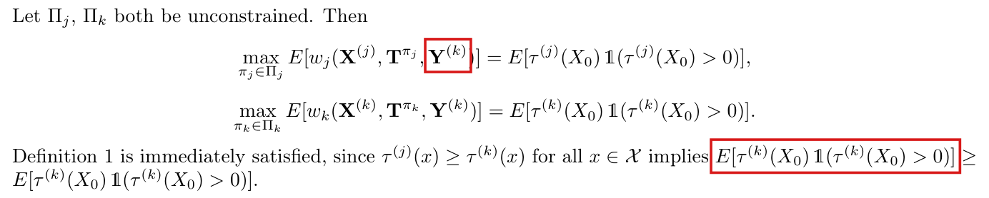
Crop of three displayed lines under the words By the tower property. First line: E of pi of X and U times mu-hat-zero of X equals E of the conditional expectation of mu-hat-zero of X sub i times pi of X sub i and U sub i, given X sub i and U sub i. Second line: equals E of pi of X sub i and U sub i times the conditional expectation of mu-hat-zero of X sub i given X sub i and U sub i. Third line: equals E of pi of X sub i and U sub i times mu-zero of X sub i. A red outline surrounds the third line.
Proof of Theorem 3, PDF p. 22. The outline marks the last equality, which replaces E[μ^0(Xi)∣Xi,Ui]E[\hat\mu_0(X_i)\mid X_i,U_i] by μ0(Xi)\mu_0(X_i).
History of this entry
  1. Classification before my review (the classification when the audit was first completed, before I reviewed it): Moderate error.
  2. Revised. The integrability conditions were revised; the classification is unchanged (error, Moderate). How this came to light: comparing the Lean statement with the audit target exposed a gap between integrability of each weighted reward summand and finiteness of the total expected reward. Two checks confirmed a cancellation counterexample in which the weighted identity and the asserted optimality fail despite finite total expectations. Why it changed: the checked repair explicitly requires integrable treated estimator residuals, integrable gτg\tau, and integrable individual weighted summands. Integrability of the estimator at untreated evaluations is not required. The best-response and zero-regret conclusions hold under these sufficient conditions. P. M. Aronow delegated this decision to the model session that runs the audit, which adopted the amendment recommended by the two checks; this note was written by that session.

Minor (20)

Real but inconsequential, for example a misprint that does not change a result.

Adding feasibility of the policy that treats nobody repairs Theorem 4, with the conclusion that some best response has arbitrarily large regret; the printed proof assumes that treatment can be withheld.

Appendix A.2, Assumption 3, Theorem 4 and its proof, PDF p. 14

See also under Formal statements (Lean): P006-T10, P006-T11

As printed

Theorem 4. Suppose ww satisfies Assumption 3. Let S\mathcal{S} be the set of all pairs of distributions D,D′\mathcal{D},\mathcal{D}' such that the distributions of Xi,Yi(1)X_i,Y_i(1) remain unchanged between D\mathcal{D} and D′\mathcal{D}'. If for all pairs of distributions D,D′∈S\mathcal{D},\mathcal{D}'\in\mathcal{S}, ED[w(X,Tπ,Y)]=ED′[w(X,Tπ,Y)]E_{\mathcal{D}}[w(\mathbf{X},\mathbf{T}^\pi,\mathbf{Y})]=E_{\mathcal{D}'}[w(\mathbf{X},\mathbf{T}^\pi,\mathbf{Y})] for all π\pi, then regret is unbounded.

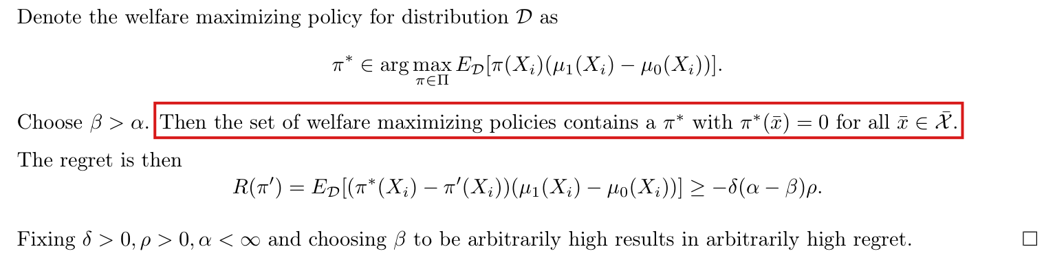
From the proof: “Choose β>α\beta>\alpha. Then the set of welfare maximizing policies contains a π∗\pi^* with π∗(xˉ)=0\pi^*(\bar x)=0 for all xˉ∈Xˉ\bar x\in\bar{\mathcal{X}}. The regret is then

R(π′)=ED[(π∗(Xi)−π′(Xi))(μ1(Xi)−μ0(Xi))]≥−δ(α−β)ρ.R(\pi')=E_{\mathcal{D}}[(\pi^*(X_i)-\pi'(X_i))(\mu_1(X_i)-\mu_0(X_i))]\ge-\delta(\alpha-\beta)\rho.

Fixing δ>0,ρ>0,α<∞\delta>0,\rho>0,\alpha<\infty and choosing β\beta to be arbitrarily high results in arbitrarily high regret.”

The problem

Section 2 measures regret against the best policy in the feasible set Π\Pi, and Theorem 4 places no condition on Π\Pi. Its proof takes a welfare-maximizing policy π∗\pi^* that does not treat on the set Xˉ\bar{\mathcal{X}}. Such a policy exists only if Π\Pi contains a policy that withholds treatment there. If Π\Pi contains only the policy that treats everyone, then that policy is both the best response and the welfare maximizer, and the regret is 00 for every distribution. The proof also takes π′\pi' and μ1\mu_1 to be constant on Xˉ\bar{\mathcal{X}}, and Assumption 3 does not supply a set of positive probability on which they are constant. The conclusion is written for the regret of a best response without saying which one, and when several policies tie, some of them can have regret 00.

Evidence an exact counterexample

The evidence is an exact counterexample and a derivation of the corrected statement. Let n=1n=1, let X=0X=0 with probability one, let Π\Pi consist of the single policy π(0)=1\pi(0)=1, and let w=wATOw=w_{\mathrm{ATO}}. For B>0B>0, let Y(1)=1Y(1)=1 and Y(0)=1+BY(0)=1+B. Assumption 3 holds because the only feasible policy treats with probability 11. For n=1n=1, I have E[wATO]=E[π(X)Y(1)]E[w_{\mathrm{ATO}}]=E[\pi(X)Y(1)], which does not involve Y(0)Y(0). The expected reward is then unchanged when the distribution of Y(0)Y(0) changes. The welfare of the only feasible policy is −B-B, which is also the maximum of the welfare over Π\Pi, and I find that the regret is 00 for every BB. With the constants of the printed proof, Xˉ={0}\bar{\mathcal{X}}=\{0\}, ρ=δ=α=1\rho=\delta=\alpha=1 and β=1+B\beta=1+B, the printed bound reads 0≥B0\ge B.

For the corrected statement, by Assumption 3 there exist a distribution D∗\mathcal{D}_* and a best response π∗\pi_* such that c=ED∗[π∗(X)]>0c=E_{\mathcal{D}_*}[\pi_*(X)]>0. For B>0B>0, let DB\mathcal{D}_B be the distribution with the same joint distribution of (X,Y(1))(X,Y(1)) as D∗\mathcal{D}_* and with Y(0)=Y(1)+BY(0)=Y(1)+B. Since the expected reward of each feasible policy is the same under DB\mathcal{D}_B and D∗\mathcal{D}_*, the policy π∗\pi_* is a best response under DB\mathcal{D}_B. Under DB\mathcal{D}_B, the treatment effect is τ(x)=−B\tau(x)=-B for all xx. Then every feasible π\pi has welfare V(π)=−B E[π(X)]≤0V(\pi)=-B\,E[\pi(X)]\le0, and the policy that treats nobody attains 00. I obtain

RDB(π∗)=0−(−Bc)=Bc,R_{\mathcal{D}_B}(\pi_*)=0-(-Bc)=Bc,

and for B=(M+1)/cB=(M+1)/c I have RDB(π∗)>MR_{\mathcal{D}_B}(\pi_*)>M. Note that the conclusion cannot be extended to every best response: with w=0w=0 and Π\Pi consisting of the policy that treats nobody and the policy that treats everyone, both policies are best responses, and for Y(1)=1Y(1)=1 and Y(0)=1+BY(0)=1+B the first has regret 00 and the second has regret BB.

What survives

Proposition 1 assumes that Π\Pi is the set of all functions π:X→[0,1]\pi:\mathcal{X}\to[0,1], and its conclusion that the regret under wATOw_{\mathrm{ATO}} can be arbitrarily large is not affected. No other result in the paper uses Theorem 4 or Assumption 3. What changes is the scope of Theorem 4 and of the two paragraphs that introduce it in Appendix A.2. The theorem does not cover a feasible set that requires some treatment, such as a fixed positive share of treated units, and it asserts large regret for some best response and not for all of them.

Corrected

Theorem 4. Suppose that the policy π≡0\pi\equiv0 belongs to Π\Pi and that ww satisfies Assumption 3. Suppose that, for every π∈Π\pi\in\Pi, the expected reward ED[w(X,Tπ,Y)]E_{\mathcal{D}}[w(\mathbf{X},\mathbf{T}^\pi,\mathbf{Y})] takes the same value for all distributions D\mathcal{D} with the same joint distribution of (Xi,Yi(1))(X_i,Y_i(1)), all expectations being finite. Then for every M>0M>0 there exist a distribution D\mathcal{D} and a best response π∗∈arg⁡max⁡π∈ΠED[w(X,Tπ,Y)]\pi_*\in\arg\max_{\pi\in\Pi}E_{\mathcal{D}}[w(\mathbf{X},\mathbf{T}^\pi,\mathbf{Y})] such that RD(π∗)>MR_{\mathcal{D}}(\pi_*)>M.

In the proof, the steps from “Let π′∈arg⁡max⁡\pi'\in\arg\max” to the regret display are replaced by the construction with Y(0)=Y(1)+BY(0)=Y(1)+B, which gives RDB(π∗)=B E[π∗(X)]R_{\mathcal{D}_B}(\pi_*)=B\,E[\pi_*(X)].

Crop of Assumption 3 (Non-degenerate w) and Theorem 4. Two red boxes mark, in the theorem, the words 'Suppose w satisfies Assumption 3.' and the words 'then regret is unbounded.'
Appendix A.2, PDF p. 14: Assumption 3 and Theorem 4. The marked hypothesis places no condition on the feasible set Π\Pi, and the marked conclusion does not say for which best response the regret is unbounded.
Crop of the second half of the proof of Theorem 4, from 'Denote the welfare maximizing policy for distribution D as' to the last line. A red box marks the sentence 'Then the set of welfare maximizing policies contains a pi star with pi star of x bar equal to 0 for all x bar in X bar.' The regret display below it ends with 'greater than or equal to minus delta times (alpha minus beta) times rho'.
Proof of Theorem 4, PDF p. 14. The marked step takes a welfare-maximizing policy that withholds treatment on Xˉ\bar{\mathcal{X}}.

In Theorem 2 the direction of absolute continuity is reversed: the weight gkg_k is defined when PX0P_{X_0} is absolutely continuous with respect to PXkP_{X^k}.

Theorem 2, PDF p. 6, foot of the left column; restatement in Appendix C.2, PDF p. 20

See also under Formal statements (Lean): P006-T5, P006-T12

As printed

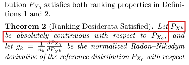
Theorem 2 (Ranking Desiderata Satisfied). Let PXk\colorbox{#ffe58a}{$P_{X^k}$} be absolutely continuous with respect to PX0\colorbox{#ffe58a}{$P_{X_0}$}, and let gk=1nkdPX0dPXkg_k=\frac{1}{n_k}\frac{dP_{X_0}}{dP_{X^k}} be the normalized Radon–Nikodym derivative of the reference distribution PX0P_{X_0} with respect to agent kk's covariate distribution PXkP_{X^k}. Then setting wkw_k to be wTTgkw_{\mathrm{TT}}^{g_k} for agent kk's treatment population satisfies both ranking properties in Definitions 1 and 2 as long as Πk\Pi_k is unconstrained and treatment effects are nonnegative, τk(x)≥0\tau^k(x)\geq0, for all k∈{1,…,K}k\in\{1,\ldots,K\}.

The problem

The derivative dPX0/dPXkdP_{X_0}/dP_{X^k} of the whole reference distribution exists when PX0P_{X_0} is absolutely continuous with respect to PXkP_{X^k}. The theorem assumes the opposite direction, which does not guarantee that the weight gkg_k is defined. Section 4 assumes that all covariate distributions have the same support X\mathcal X. If support is understood in the topological sense, this assumption does not supply the missing direction. The intended condition is clear from the derivative that the theorem names, and with it the change-of-measure argument is valid.

Evidence an exact counterexample

The evidence is an exact counterexample to the sufficiency of the printed condition, and a derivation of the theorem under the corrected one.

Counterexample. On [0,1][0,1], let LL be Lebesgue measure, and let PXk=LP_{X^k}=L and PX0=(L+δ1/2)/2P_{X_0}=(L+\delta_{1/2})/2. For every Borel set CC, I have PX0(C)≥PXk(C)/2P_{X_0}(C)\ge P_{X^k}(C)/2, which implies that PXkP_{X^k} is absolutely continuous with respect to PX0P_{X_0}, as the theorem assumes. Both distributions have support [0,1][0,1]. However, PXk({1/2})=0P_{X^k}(\{1/2\})=0 and PX0({1/2})=1/2P_{X_0}(\{1/2\})=1/2. If a density f=dPX0/dPXkf=dP_{X_0}/dP_{X^k} existed, then I would have 1/2=PX0({1/2})=∫{1/2}f dPXk=01/2=P_{X_0}(\{1/2\})=\int_{\{1/2\}}f\,dP_{X^k}=0. The example shows that the printed condition does not suffice for the construction. It is not a counterexample to the ranking conclusion in a case where the derivative exists.

Derivation. Suppose that PX0P_{X_0} is absolutely continuous with respect to PXkP_{X^k}, and write f=dPX0/dPXkf=dP_{X_0}/dP_{X^k}, so that gk=f/nkg_k=f/n_k. Then ∫h dPX0=∫hf dPXk\int h\,dP_{X_0}=\int hf\,dP_{X^k} for every nonnegative measurable function hh. Using the expected score of Theorem 1 and this identity with h=τkπkh=\tau^k\pi_k, I obtain

E[wk]=nk∫τk(x)πk(x)gk(x) dPXk(x)=∫τk(x)πk(x) dPX0(x).E[w_k]=n_k\int\tau^k(x)\pi_k(x)g_k(x)\,dP_{X^k}(x)=\int\tau^k(x)\pi_k(x)\,dP_{X_0}(x).

Since 0≤πk≤10\le\pi_k\le1 and τk≥0\tau^k\ge0, the maximum over πk\pi_k is E[τk(X0)]E[\tau^k(X_0)], attained at πk≡1\pi_k\equiv1. If τj(x)≥τk(x)\tau^j(x)\ge\tau^k(x) for all xx, then E[τj(X0)]≥E[τk(X0)]E[\tau^j(X_0)]\ge E[\tau^k(X_0)], and Definition 1 holds. The hypothesis of Definition 2 is this inequality itself.

What survives

The ranking conclusion and its proof are unchanged once the condition is reversed. Theorem 1, the results of Sections 3 and 5 and the experiments of Section 6 do not use the condition. Section 6 contains no experiment with reweighting to a reference distribution. The expected score used in the derivation requires the corrected Assumption 1 of P006-E002.

Corrected

Theorem 2 (Ranking Desiderata Satisfied). Let PX0\colorbox{#ffe58a}{$P_{X_0}$} be absolutely continuous with respect to PXk\colorbox{#ffe58a}{$P_{X^k}$}, and let gk=1nkdPX0dPXkg_k=\frac{1}{n_k}\frac{dP_{X_0}}{dP_{X^k}} be the normalized Radon–Nikodym derivative of the reference distribution PX0P_{X_0} with respect to agent kk's covariate distribution PXkP_{X^k}. Then setting wkw_k to be wTTgkw_{\mathrm{TT}}^{g_k} for agent kk's treatment population satisfies both ranking properties in Definitions 1 and 2 as long as Πk\Pi_k is unconstrained and treatment effects are nonnegative, τk(x)≥0\tau^k(x)\geq0, for all k∈{1,…,K}k\in\{1,\ldots,K\}.

The same change applies to the restatement on PDF p. 20, where the distribution is written PX(k)P_{X^{(k)}}. If the weights gkg_k must also be strictly positive almost everywhere under PXkP_{X^k}, as the proof of Theorem 1 assumes of its weight, then the two distributions must be mutually absolutely continuous. The ranking conclusion does not need this.

Crop of six lines of the left column. Two lines end a paragraph: bution P sub X sub 0 satisfies both ranking properties in Definitions 1 and 2. Then: Theorem 2 (Ranking Desiderata Satisfied). Let P sub X superscript k be absolutely continuous with respect to P sub X sub 0, and let g sub k equal one over n sub k times d P sub X sub 0 over d P sub X superscript k be the normalized Radon-Nikodym derivative of the reference distribution P sub X sub 0 with respect. Red outlines surround P sub X superscript k and the words be absolutely continuous with respect to P sub X sub 0.
Theorem 2, PDF p. 6, foot of the left column; the statement continues at the top of the right column. The outlines mark the condition of absolute continuity.
Crop of three lines. The text reads: Theorem 2 (Ranking Desiderata Satisfied). Let P sub X superscript (k) be absolutely continuous with respect to P sub X sub 0, and let g sub k equal one over n sub k times d P sub X sub 0 over d P sub X superscript (k) be the normalized Radon-Nikodym derivative of the reference distribution P sub X sub 0 with respect to agent k's covariate distribution P sub X superscript (k). Then. A red outline surrounds the words from P sub X superscript (k) to P sub X sub 0.
Restatement of Theorem 2 in Appendix C.2, PDF p. 20. The outline marks the same condition.

The positivity condition of Appendix D.3 and Theorem 5 is that untreated units occur with positive probability at each xx, P(Tπ=0∣X=x)>0P(T^\pi=0\mid X=x)>0, for which π(x,u)<1\pi(x,u)<1 suffices; the printed condition π>0\pi>0 concerns the treated units.

Appendix D.3, first paragraph and Theorem 5, PDF p. 23; proof of Theorem 5, sentence before Lemma 3, PDF p. 24

See also under Formal statements (Lean): P006-T15, P006-T16

As printed

Appendix D.3, first paragraph, PDF p. 23: “As discussed in Sections 5 and A, under full information symmetry, the mean conditional untreated potential outcome is identifiable as long as the agent’s treatment rule class Π\Pi maintains positivity, π(x)>0\pi(x)>0 for all x∈Xx\in\mathcal{X}.”

PDF p. 23: “Theorem 5. Suppose for all π∈Π\pi\in\Pi, π(x,u)>0\pi(x,u)>0 for all x∈Xx\in\mathcal{X}, u∈Uu\in\mathcal{U}. If the principal applies the reward function wTTw_{\mathrm{TT}} using an estimate μ^0π(x)\hat\mu_0^\pi(x), then under Assumption 4, the regret is upper bounded as R(πw)≤2γmax⁡R(\pi^w)\le2\gamma_{\max}.”

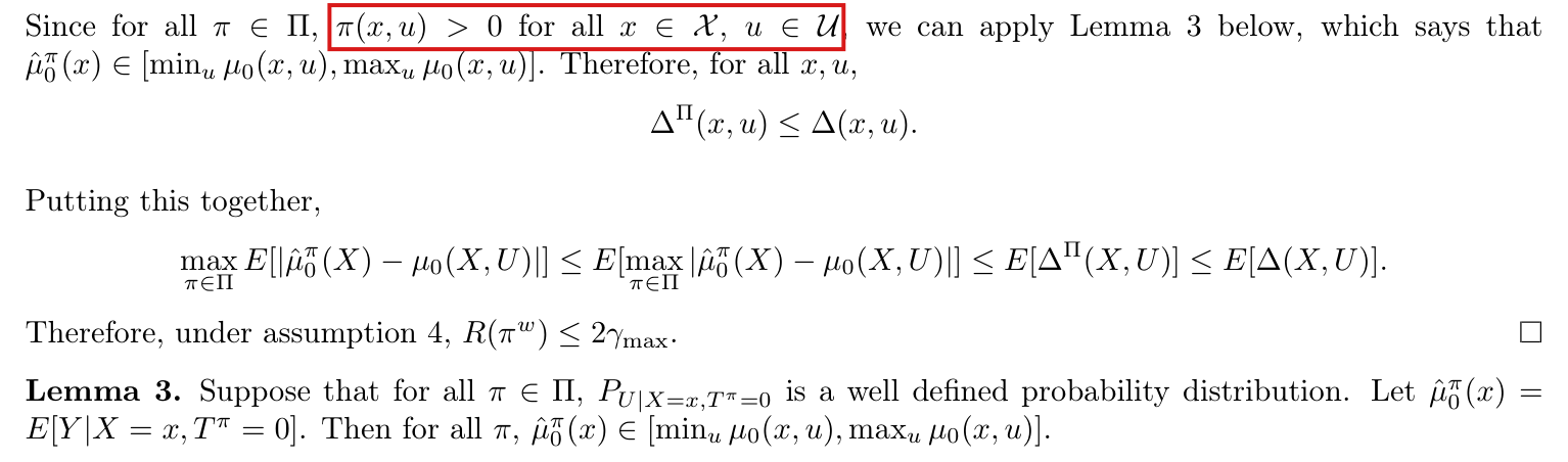
Proof, PDF p. 24: “Since for all π∈Π\pi\in\Pi, π(x,u)>0\pi(x,u)>0 for all x∈Xx\in\mathcal{X}, u∈Uu\in\mathcal{U}, we can apply Lemma 3 below, which says that μ^0π(x)∈[min⁡uμ0(x,u),max⁡uμ0(x,u)]\hat\mu_0^\pi(x)\in[\min_u\mu_0(x,u),\max_u\mu_0(x,u)].”

The problem

In the paper π\pi is the probability of treatment. The estimate μ^0π(x)=E[Yi∣Tπ=0,X=x]\hat\mu_0^\pi(x)=E[Y_i\mid T^\pi=0,X=x] is a mean over untreated units. It is defined only if untreated units occur with positive probability at xx, and Lemma 3 assumes that the distribution of UU given X=xX=x and Tπ=0T^\pi=0 is well defined. The printed condition π>0\pi>0 ensures instead that treated units occur, and it allows a policy that treats everyone. The condition is printed in this form in three places. Appendix A.1 states the condition correctly, as P(Tiπ=0∣Xi=x)>0P(T_i^\pi=0\mid X_i=x)>0, and notes that it can be enforced by restricting Π\Pi to treatment rules with π(x)<1\pi(x)<1.

Evidence an exact counterexample

The evidence is an exact counterexample to the printed hypothesis and a derivation of the bound under the corrected one. Let X=0X=0 and U=0U=0 with probability one, let Π\Pi consist of the single policy π(0,0)=1\pi(0,0)=1, and let Y(1)=1Y(1)=1. Consider Y(0)=0Y(0)=0 and Y(0)=2Y(0)=2. In both cases π>0\pi>0, Assumption 4 holds with γmax⁡=0\gamma_{\max}=0, and the observed data are the single point (X,T,Y)=(0,1,1)(X,T,Y)=(0,1,1). The untreated means are 00 and 22, and the untreated mean is not identified. Further, P(Tπ=0∣X=0)=0P(T^\pi=0\mid X=0)=0, and the conditional mean in μ^0π(0)\hat\mu_0^\pi(0) is the ratio 0/00/0. Untreated units elsewhere do not help: with P(X=0)=P(X=1)=1/2P(X=0)=P(X=1)=1/2, π(0)=1\pi(0)=1 and π(1)=1/2\pi(1)=1/2, I have P(Tπ=0)=1/4P(T^\pi=0)=1/4 and P(Tπ=0∣X=0)=0P(T^\pi=0\mid X=0)=0.

For the corrected hypothesis, I write qπ(x)=P(Tπ=0∣X=x)=E[1−π(x,U)∣X=x]q_\pi(x)=P(T^\pi=0\mid X=x)=E[1-\pi(x,U)\mid X=x] and suppose that qπ(x)>0q_\pi(x)>0. Then the distribution of UU given X=xX=x and Tπ=0T^\pi=0 has density (1−π(x,u))/qπ(x)(1-\pi(x,u))/q_\pi(x) with respect to the distribution of UU given X=xX=x, and μ^0π(x)\hat\mu_0^\pi(x) is the mean of μ0(x,⋅)\mu_0(x,\cdot) under it. This implies that ∣μ^0π(x)−μ0(x,u)∣≤Δ(x,u)|\hat\mu_0^\pi(x)-\mu_0(x,u)|\le\Delta(x,u) for all uu, where Δ(x,u)=max⁡u~∈U∣μ0(x,u)−μ0(x,u~)∣\Delta(x,u)=\max_{\tilde u\in\mathcal{U}}|\mu_0(x,u)-\mu_0(x,\tilde u)| is the quantity defined in Assumption 4. Let S(π)=E[π(X,U)(μ1(X,U)−μ^0π(X))]S(\pi)=E[\pi(X,U)(\mu_1(X,U)-\hat\mu_0^\pi(X))] denote the expected reward per unit. Since 0≤π≤10\le\pi\le1, I have ∣S(π)−V(π)∣≤E[Δ(X,U)]≤γmax⁡|S(\pi)-V(\pi)|\le E[\Delta(X,U)]\le\gamma_{\max} for every π∈Π\pi\in\Pi. Let π∗\pi^* maximize VV over Π\Pi. Since πw\pi^w maximizes SS over Π\Pi, I obtain

R(πw)=[V(π∗)−S(π∗)]+[S(π∗)−S(πw)]+[S(πw)−V(πw)]≤2γmax⁡.R(\pi^w)=[V(\pi^*)-S(\pi^*)]+[S(\pi^*)-S(\pi^w)]+[S(\pi^w)-V(\pi^w)]\le2\gamma_{\max}.
What survives

The bound R(πw)≤2γmax⁡R(\pi^w)\le2\gamma_{\max} of Theorem 5 holds under the corrected hypothesis, with the same constant, and Lemma 3 holds under its own hypothesis. The results of Appendix D.2, Theorem 3 and Proposition 5 do not use the condition. Appendix E.3 states that the experiments do not simulate the estimation of μ^0\hat\mu_0 from a subset of the data, and no reported number depends on the condition. The corrected hypothesis restricts Π\Pi: it excludes every policy that treats all units at a value of xx of positive probability. Appendix A.1 notes that such a restriction may not always be possible or ethical.

Corrected

Appendix D.3, first paragraph: “… the mean conditional untreated potential outcome is identifiable as long as the agent’s treatment rule class Π\Pi maintains positivity, π(x)<1\pi(x)<1 for all x∈Xx\in\mathcal{X}.”

Theorem 5. Suppose for all π∈Π\pi\in\Pi, P(Tπ=0∣X=x)=E[1−π(x,U)∣X=x]>0P(T^\pi=0\mid X=x)=E[1-\pi(x,U)\mid X=x]>0 for almost every xx with respect to the distribution of XX. If the principal applies the reward function wTTw_{\mathrm{TT}} using the estimate μ^0π(x)=E[Yi∣Tπ=0,X=x]\hat\mu_0^\pi(x)=E[Y_i\mid T^\pi=0,X=x], then under Assumption 4, the regret is upper bounded as R(πw)≤2γmax⁡R(\pi^w)\le2\gamma_{\max}. The hypothesis holds if π(x,u)<1\pi(x,u)<1 for all x∈Xx\in\mathcal{X}, u∈Uu\in\mathcal{U}.

Proof: “Since for all π∈Π\pi\in\Pi, P(Tπ=0∣X=x)>0P(T^\pi=0\mid X=x)>0 for almost every xx with respect to the distribution of XX, the distribution PU∣X=x,Tπ=0P_{U\mid X=x,T^\pi=0} is well defined and we can apply Lemma 3 below …”

Crop of the first paragraph of Appendix D.3, six lines, beginning 'Suppose the principal estimates mu hat 0 of x from the untreated data from the agent's treatment population'. A red box marks 'pi of x greater than 0 for all x in X' after the words 'maintains positivity'.
Appendix D.3, first paragraph, PDF p. 23. The marked condition is stated as positivity for identifying the untreated outcome from the agent’s untreated units.
Crop of the statement of Theorem 5 with its display 'R of pi w is at most 2 gamma max'. A red box marks the hypothesis 'pi of x, u greater than 0 for all x in X, u in U'.
Theorem 5, PDF p. 23. The marked hypothesis requires a positive probability of treatment.
Crop of the end of the proof of Theorem 5 and the statement of Lemma 3. A red box marks 'pi of x, u greater than 0 for all x in X, u in U' in the sentence 'Since for all pi in Pi, ..., we can apply Lemma 3 below'. Lemma 3 begins 'Suppose that for all pi in Pi, P of U given X equals x and T pi equals 0 is a well defined probability distribution.'
Proof of Theorem 5, PDF p. 24. The marked condition is given as the reason that Lemma 3 applies. Lemma 3, at the bottom of the crop, assumes that the distribution of UU given X=xX=x and Tπ=0T^\pi=0 is well defined.

The sentence beginning “Intuitively” refers to Assumption 2 and not Assumption 4, and the agent concentrates the estimate μ^0π(x)\hat\mu_0^\pi(x) on one type u~\tilde u by leaving only that type untreated, not by treating only that type.

Appendix D.3, paragraph after Assumption 4, sentence beginning “Intuitively”, PDF p. 23

See also under Formal statements (Lean): P006-T17

As printed

Assumption 4 is stronger than Assumption 2 in the sense that Assumption 2 is not sufficient to bound the regret when the principal estimates the mean conditional untreated potential outcome from the agent’s data using μ^0π(X)\hat\mu_0^\pi(X). Furthermore, the bound in Assumption 4 implies that Assumption 2 is satisfied with γmarg≤γmax⁡\gamma_{\mathrm{marg}}\le\gamma_{\max}. Intuitively, Assumption 4 is not sufficient to bound the regret when the principal uses μ^0π(X)\hat\mu_0^\pi(X) because the agent can choose π\pi to allocate treatment to single values of u~∈U\tilde u\in\mathcal{U}, such that μ^0π(x)\hat\mu_0^\pi(x) ends up matching a single value μ0(x,u~)\mu_0(x,\tilde u).

The problem

The sentence means Assumption 2: the preceding sentence says that Assumption 2 is not sufficient, and Theorem 5, which follows, shows that Assumption 4 is sufficient. Since the estimate μ^0π(x)=E[Yi∣Tπ=0,X=x]\hat\mu_0^\pi(x)=E[Y_i\mid T^\pi=0,X=x] is a mean over the untreated units, it equals μ0(x,u~)\mu_0(x,\tilde u) when the type u~\tilde u is the only one left untreated, not when it is the only one treated.

Evidence a derivation

This is a check of the page and a short computation. If UU takes finitely many values with conditional probabilities pup_u given X=xX=x, then μ^0π(x)=∑uμ0(x,u)pu(1−π(x,u))/∑upu(1−π(x,u))\hat\mu_0^\pi(x)=\sum_u\mu_0(x,u)p_u(1-\pi(x,u))/\sum_up_u(1-\pi(x,u)). For three equally likely types with μ0(x,u)\mu_0(x,u) equal to 00, 11 and 33, I find μ^0π(x)=2\hat\mu_0^\pi(x)=2 when only the first type is treated, and μ^0π(x)=0\hat\mu_0^\pi(x)=0 when only the first type is left untreated.

What survives

No result depends on this sentence; the hypothesis of Theorem 5 is the subject of P006-E006.

Corrected

Intuitively, Assumption 2 is not sufficient to bound the regret when the principal uses μ^0π(X)\hat\mu_0^\pi(X), because the agent can leave only a selected type u~\tilde u of positive conditional probability untreated, so that μ^0π(x)=μ0(x,u~)\hat\mu_0^\pi(x)=\mu_0(x,\tilde u).

Crop of the six-line paragraph beginning 'Assumption 4 is stronger than Assumption 2'. In its last sentence, two red boxes mark the words 'Assumption 4' after 'Intuitively,' and the words 'allocate treatment to single values of u tilde in U'.
Appendix D.3, paragraph after Assumption 4, PDF p. 23. The first mark is the assumption named in the sentence beginning “Intuitively”. The second mark is the description of the agent’s policy.

The regret in the second failure mode is (1−p)−p(1−β)=1−2p+pβ(1-p)-p(1-\beta)=1-2p+p\beta; the printed display subtracts p(β−1)p(\beta-1) and has the value 1−pβ1-p\beta.

Appendix B.4, proof of Proposition 1, second failure mode, display after “Then the regret is given by”, PDF p. 17

See also under Formal statements (Lean): P006-T18, P006-T19

As printed

A second failure mode would be if α=−1\alpha=-1, and β>1\beta>1. Then the regret is given by

R(πw)=(1−p)−p(β−1)=1−pβ.R(\pi^w)=(1-p)\colorbox{#ffe58a}{$\displaystyle {}-p(\beta-1)=1-p\beta$}.

This is also unbounded for unbounded β\beta.

The problem

For 0<p<10<p<1, the proof takes X={0,1}\mathcal{X}=\{0,1\} with P(Xi=1)=pP(X_i=1)=p, μ1(0)=0\mu_1(0)=0, μ1(1)=1\mu_1(1)=1, μ0(0)=α\mu_0(0)=\alpha and μ0(1)=β\mu_0(1)=\beta, and the agent’s policy πw(0)=0\pi^w(0)=0, πw(1)=1\pi^w(1)=1. The regret is the largest welfare minus the welfare of πw\pi^w. In the second failure mode the welfare of πw\pi^w is p(1−β)p(1-\beta), which is negative. The display subtracts p(β−1)p(\beta-1), its absolute value. The printed expression 1−pβ1-p\beta decreases in β\beta and is negative for β>1/p\beta>1/p, and a regret is never negative.

Evidence an exact counterexample

The evidence is a derivation and an exact example. With α=−1\alpha=-1 and β>1\beta>1, the treatment effects are τ(0)=0−(−1)=1\tau(0)=0-(-1)=1 and τ(1)=1−β<0\tau(1)=1-\beta<0, which yields V(π)=(1−p)π(0)+p(1−β)π(1)V(\pi)=(1-p)\pi(0)+p(1-\beta)\pi(1). For every policy,

(1−p)−V(π)=(1−p)(1−π(0))+p(β−1)π(1)≥0,(1-p)-V(\pi)=(1-p)(1-\pi(0))+p(\beta-1)\pi(1)\ge0,

which implies that the largest welfare is 1−p1-p, attained by treating x=0x=0 only. The agent’s policy has V(πw)=p(1−β)V(\pi^w)=p(1-\beta). I obtain

R(πw)=(1−p)−p(1−β)=1−2p+pβ,R(\pi^w)=(1-p)-p(1-\beta)=1-2p+p\beta,

which exceeds the printed expression by 2p(β−1)>02p(\beta-1)>0. For p=1/2p=1/2 and β=4\beta=4, the largest welfare is 1/21/2, the welfare of πw\pi^w is −3/2-3/2, and the regret is 22; the printed expression equals −1-1. In this example with n=2n=2, a direct enumeration shows that πw\pi^w maximizes the expected reward under wATOw_{\mathrm{ATO}} as defined. The example does not depend on the rule corrected in P006-E001.

What survives

Proposition 1 is unchanged. With p=1/2p=1/2 and β=2m\beta=2m, the corrected regret equals mm. The regret in the second failure mode is then unbounded, and the first failure mode, with regret −α(1−p)-\alpha(1-p), is printed correctly. The replication files compute the regret under wATOw_{\mathrm{ATO}} as the difference between the largest utility and the utility of the agent’s policy, both computed from μ1−μ0\mu_1-\mu_0, and no reported number depends on this display.

Corrected

Let X={0,1}\mathcal{X}=\{0,1\} with P(Xi=1)=pP(X_i=1)=p, 0<p<10<p<1, μ1(0)=0\mu_1(0)=0, μ1(1)=1\mu_1(1)=1, μ0(0)=α=−1\mu_0(0)=\alpha=-1 and μ0(1)=β>1\mu_0(1)=\beta>1, and let πw(0)=0\pi^w(0)=0 and πw(1)=1\pi^w(1)=1. Then the regret is given by

R(πw)=(1−p)−p(1−β)=1−2p+pβ.R(\pi^w)=(1-p)-p(\colorbox{#ffe58a}{$\displaystyle 1-\beta$})=\colorbox{#ffe58a}{$\displaystyle 1-2p+p\beta$}.

This is also unbounded for unbounded β\beta.

Crop of the paragraph 'A second failure mode would be if alpha equals minus 1, and beta is greater than 1. Then the regret is given by', the display, and the three lines that follow. A red box marks the right part of the display, 'minus p times (beta minus 1) equals 1 minus p beta', which follows 'R of pi w equals (1 minus p)'.
Appendix B.4, proof of Proposition 1, PDF p. 17: the second failure mode. The marked terms are the welfare of the agent’s policy, entered with the wrong sign, and the resulting value of the regret.

With survival coded 11 and death coded −1-1, the fitted conditional mean is μt(x)=2σ(⋅)−1\mu_t(x) = 2\sigma(\cdot) - 1 and not the survival probability σ(⋅)\sigma(\cdot) that the appendix prints; the released code uses the correct formula.

Appendix E.2.1, paragraph beginning “We trained a logistic regression model” (PDF p. 25)

See also under Formal statements (Lean): P006-T20, P006-T21

As printed

We removed all examples in which the horse was euthanized, and used the remaining “outcome” variable as YY, where we set Yi=1Y_i = 1 if the horse lived, and Yi=−1Y_i = -1 if the horse died. […] To simulate μt(x)\mu_t(x), we assume that the outcome distribution takes the parametric form,

P(Y(t)=1∣X=x)=σ(β0+β1⊤x+β2t+β3⊤xt)P(Y(t) = 1 | X = x) = \sigma(\beta_0 + \beta_1^\top x + \beta_2 t + \beta_3^\top x t)

where σ(x)=11+e−x\sigma(x) = \frac{1}{1+e^{-x}} is the standard logistic function.

We trained a logistic regression model of YY on XX, TT, and the interaction term XTXT to estimate parameters β^\hat\beta, and used the resulting estimate to compute μt(x)=σ(β^0+β^1⊤x+β^2t+β^3⊤xt)\mu_t(x) = \colorbox{#ffe58a}{$\sigma(\hat\beta_0 + \hat\beta_1^\top x + \hat\beta_2 t + \hat\beta_3^\top x t)$}. […] When computing agent best responses and regret, we take this function μt(x)\mu_t(x) to be given as synthetic mean conditional potential outcomes.

The problem

The appendix codes YY on the scale {−1,1}\{-1, 1\}, and Section 2 defines μt(X)\mu_t(X) as the conditional mean E[Yi(t)∣X]\mathbb{E}[Y_i(t) \mid X]. The logistic model specifies the probability of survival, P(Y(t)=1∣X=x)P(Y(t) = 1 \mid X = x), and the printed sentence sets the mean equal to that probability. For an outcome with the values 11 and −1-1, the mean is twice the probability minus one. The two agree only if the probability is one, a value that the logistic function does not attain. The released notebook computes the means as 2p−12p - 1 from the fitted probability pp. The numbers in the paper are then on the stated scale, and the defect is in the description. If the printed formula were followed, the treatment effects would be half as large, and so would the utility and the regret of a fixed treatment rule. The response to the total-outcome reward wTOw_{\mathrm{TO}} of the appendix could also change. Its rule μ1(x)>0\mu_1(x) > 0 means P(Y(1)=1∣X=x)>1/2P(Y(1) = 1 \mid X = x) > 1/2 on the stated scale, and it holds for every xx when the mean is replaced by the probability.

Evidence an exact counterexample

The evidence is a derivation and an exact counterexample. Fix tt and xx, and write pt(x)=P(Y(t)=1∣X=x)p_t(x) = P(Y(t) = 1 \mid X = x). Since Y(t)Y(t) takes only the values 11 and −1-1, I have

E[Y(t)∣X=x]=1⋅pt(x)+(−1)⋅(1−pt(x))=2pt(x)−1.\mathbb{E}[Y(t) \mid X = x] = 1 \cdot p_t(x) + (-1) \cdot (1 - p_t(x)) = 2 p_t(x) - 1 .
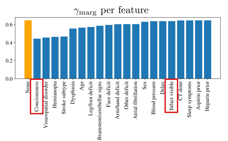
Substituting the fitted probability into this identity, I obtain the corrected formula. For the counterexample, let X=0X = 0 with probability one, and let (Y(0),Y(1))(Y(0), Y(1)) equal (1,1)(1, 1), (1,−1)(1, -1), (−1,1)(-1, 1) and (−1,−1)(-1, -1) with probabilities 1/81/8, 3/83/8, 1/81/8 and 3/83/8. This law belongs to the printed model, with β0=0\beta_0 = 0, β2=−log⁡3\beta_2 = -\log 3 and β1=β3=0\beta_1 = \beta_3 = 0: the survival probabilities are σ(0)=1/2\sigma(0) = 1/2 without treatment and σ(−log⁡3)=1/4\sigma(-\log 3) = 1/4 with treatment. The means are μ0=0\mu_0 = 0 and μ1=−1/2\mu_1 = -1/2, and the printed formula gives μ1=1/4\mu_1 = 1/4. In this example the rule μ1(x)>0\mu_1(x) > 0 treats nobody when the correct mean is used and everybody when the printed one is used. The first response has regret 00, and the second has regret 1/21/2. In the released notebook for the Horse Colic data, both prediction functions return (Y_probs*2.) - 1., and the optimal utility stored there, 0.1469540.146954, agrees with the entry 0.146950.14695 of Table 1.

What survives

The correction changes one formula in the description of the experiment. It adds no assumption and changes no estimand or theorem. The released code already applies it. The Horse Colic entries of Tables 1 and 2 need no change for this correction, and they should not be doubled. The probability equations in Section 6 and in the appendix are correct as printed, and the Stroke Trial model and the theoretical results do not involve this formula.

Corrected

We trained a logistic regression model of YY on XX, TT, and the interaction term XTXT to estimate parameters β^\hat\beta, and used the resulting estimate to compute

μt(x)=2 σ(β^0+β^1⊤x+β^2t+β^3⊤xt)−1.\mu_t(x) = \colorbox{#ffe58a}{$\displaystyle 2$}\,\sigma(\hat\beta_0 + \hat\beta_1^\top x + \hat\beta_2 t + \hat\beta_3^\top x t) \colorbox{#ffe58a}{$\displaystyle {} - 1$} .

Here Yi=1Y_i = 1 if the horse lived and Yi=−1Y_i = -1 if the horse died, and σ(β^0+β^1⊤x+β^2t+β^3⊤xt)\sigma(\hat\beta_0 + \hat\beta_1^\top x + \hat\beta_2 t + \hat\beta_3^\top x t) is the fitted probability P(Y(t)=1∣X=x)P(Y(t) = 1 \mid X = x) of survival. The two probability equations, in Section 6 (PDF p. 7) and in Appendix E.2.1, stay as printed, and Section 6 may state the same conversion to the mean.

Crop of eleven lines of Appendix E.2.1. The text reads: We removed all examples in which the horse was euthanized, and used the remaining outcome variable as Y, where we set Y sub i = 1 if the horse lived, and Y sub i = -1 if the horse died. After a sentence on the data files it continues: To simulate mu sub t of x, we assume that the outcome distribution takes the parametric form, P(Y(t) = 1 given X = x) = sigma(beta 0 + beta 1 transpose x + beta 2 t + beta 3 transpose x t), where sigma(x) = 1 over (1 + e to the minus x) is the standard logistic function. We trained a logistic regression model of Y on X, T, and the interaction term XT to estimate parameters beta hat, and used the resulting estimate to compute mu sub t of x = sigma(beta hat 0 + beta hat 1 transpose x + beta hat 2 t + beta hat 3 transpose x t). A red outline surrounds this last formula. The crop also shows the AUC and accuracy, the statement that mu sub t of x is taken as synthetic mean conditional potential outcomes, and the beginning of a sentence on clinical validity.
Appendix E.2.1 (PDF p. 25). The outline marks the printed formula for μt(x)\mu_t(x). Its right side is the survival probability of the display above it, and the second line of the crop codes the outcome as 11 and −1-1.

The numbers 0.147 and 0.025 are averages of the positive fitted effects over all horses and all patients in the analysis samples; among the horses and patients that would benefit, the average fitted benefit is about 0.604 and 0.135.

Section 6, paragraph “Horse Colic dataset”, PDF p. 7, right column; paragraph “International Stroke Trial dataset”, PDF p. 8, top of the left column

See also under Formal statements (Lean): P006-T9, P006-T28

As printed

PDF p. 7. The fitted μ0(x)\mu_0(x) and μ1(x)\mu_1(x) show 62 horses benefiting from surgery and 146 being better off without surgery. On the horses that would benefit, the average benefit was 0.147, which is fairly significant.

PDF pp. 7–8. The fitted μ0(x)\mu_0(x) and μ1(x)\mu_1(x) showed 1360 patients benefiting from heparin and 5904 being better off without heparin. On the patients that would benefit, the average benefit of treatment was 0.025. This tracks with the study’s findings that the benefit of heparin was non-significant and inconclusive.

The problem

The two sentences describe 0.147 and 0.025 as averages over the units that would benefit, that is, over the 62 horses and the 1360 patients whose fitted effect μ1(x)−μ0(x)\mu_1(x)-\mu_0(x) is positive. The released notebooks compute a different quantity. They multiply each fitted effect by the indicator that it is positive and take the mean over the whole analysis sample: V_OPT = ((mu_1s - mu_0s)* T_OPT).mean(), where T_OPT is the indicator. The units with a fitted effect that is not positive enter this mean as zeros. The stored values are 0.146954 for the 255 horses and 0.025186 for the 7264 patients, and they are the wTTw_{\mathrm{TT}} utilities of Table 1 (0.14695 and 0.02518). The average over the units that would benefit divides the same sums by 62 and by 1360. It is larger than the printed number by the factors 255/62≈4.1255/62\approx4.1 and 7264/1360≈5.37264/1360\approx5.3.

Evidence a historical Lean attribution (Generated status: clause support not certified in this release)

The evidence is a recalculation from the stored outputs of the released notebooks, in exact arithmetic. Let τ^i=μ1(Xi)−μ0(Xi)\hat\tau_i=\mu_1(X_i)-\mu_0(X_i) for the nn units of the analysis sample, let kk be the number of units with τ^i>0\hat\tau_i>0, and let SS be the sum of τ^i\hat\tau_i over those units. The notebooks compute V=S/nV=S/n. The average over the units that would benefit is

b=Sk=V⋅nk.b=\frac{S}{k}=V\cdot\frac{n}{k}.

The stored values of VV are rounded to six decimals. Allowing for this rounding, I obtain the intervals in the table.

The printed numbers and the averages over the units that would benefit.
Data setnnkkV=S/nV=S/n (printed as 0.147 and 0.025)b=S/kb=S/k
Horse Colic255620.146954between 0.604405 and 0.604410
Stroke Trial726413600.025186between 0.134520 and 0.134526

Neither interval contains a number that rounds to 0.147 or to 0.025. The identity for bb and the two intervals are also proved in Lean, with the stored values and the sample sizes as hypotheses. For an independent least-squares fit of the Stroke model, I find the counts 1360 and 5904 again, with V=0.025185778762V=0.025185778762 and b=0.134521688917b=0.134521688917. The Horse Colic model was not fitted again. Its value of bb follows from the stored outputs.

What survives

The utility VV as defined in Section 2, Table 1’s interpretation as population utilities and regrets, and the theoretical results require no change because of this wording error. If the numbers are kept, then the remarks that follow them (“fairly significant”, and the comparison with the trial’s finding on heparin) refer to gains averaged over the whole samples. These are fitted effects of a synthetic model, and my check does not establish clinical or statistical significance.

Corrected

PDF p. 7. … Under the fitted model, treating only the horses with positive fitted effects gives an average welfare gain of 0.147 over all 255 horses in the analysis sample, with zero contributions from the horses not treated.

PDF pp. 7–8. … Under the fitted model, treating only the patients with positive fitted effects gives an average welfare gain of 0.025 over all 7264 patients in the analysis sample, with zero contributions from the patients not treated.

Alternatively, the two sentences keep their wording and the numbers become 0.604 and 0.135. In general, if r>0r\colorbox{#ffe58a}{$>0$} is the fraction of units with a positive fitted effect and V∗V^* is the unconstrained optimal utility, then the mean fitted benefit among those units is V∗/rV^*/r.

Crop of eight lines of the right column. The text reads: take these as given to produce mu-zero of x and mu-one of x. The fitted mu-zero of x and mu-one of x show 62 horses benefiting from surgery and 146 being better off without surgery. On the horses that would benefit, the average benefit was 0.147, which is fairly significant. The clinical validity of these estimated potential outcomes cannot be verified from this data alone, and we instead take these estimates as synthetic potential outcomes. Red outlines surround the words the horses that would benefit and the number 0.147.
Section 6, paragraph “Horse Colic dataset”, PDF p. 7, right column. The outlines mark the group to which the average is attributed and the number.
Crop of five lines of the left column. The text reads: 1360 patients benefiting from heparin and 5904 being better off without heparin. On the patients that would benefit, the average benefit of treatment was 0.025. This tracks with the study's findings that the benefit of heparin was non-significant and inconclusive. Red outlines surround the words the patients that would benefit, which run over a line break, and the number 0.025.
Section 6, paragraph “International Stroke Trial dataset”, PDF p. 8, top of the left column. The outlines mark the group to which the average is attributed and the number.
Two bar charts side by side under the title: The printed averages are taken over the whole sample, not over the units that would benefit. Left panel, Horse Colic (surgery): a blue bar of height 0.147 labelled all 255 horses and an orange bar of height 0.604 labelled the 62 horses that would benefit. Right panel, Stroke Trial (heparin): a blue bar of height 0.025 labelled all 7264 patients and an orange bar of height 0.135 labelled the 1360 patients that would benefit. A legend says that blue is the average over the whole analysis sample (the printed number) and orange the average over the units with a positive fitted effect. The vertical axis is the average fitted benefit of treatment in units of the outcome Y.
The printed numbers (blue) and the averages over the units that would benefit (orange), from the stored outputs of the released notebooks. The two panels have different vertical scales, since the outcome is ±1\pm1 for the Horse Colic data and a score between −4-4 and 33 for the Stroke data.

The accuracy 0.68240.6824 reported for the outcome model of the Horse Colic data is the share of horses that were predicted to live and did live, 174/255174/255, because the code compares predictions coded 00 and 11 with outcomes coded −1-1 and 11; the correctly scored accuracy of the same fit is at least 199/255≈0.7804199/255 \approx 0.7804, and it is 246/255≈0.9647246/255 \approx 0.9647 in a reconstruction of the fit.

Appendix E.2.1, sentence “For the fitted model, the AUC was 0.9924, and the accuracy was 0.6824” (PDF p. 25); Horse Colic notebook of the replication files, eighth cell, methods fit_outcome and print_metrics

As printed

Appendix E.2.1. For the fitted model, the AUC was 0.9924, and the accuracy was 0.6824.

Notebook horse_colic_experiments.ipynb, method fit_outcome (an excerpt: the lines between those shown and the arguments of the constructor are omitted, and the print statement is broken here after the format string).

target = self.get_target_column(df_input)clf_outcome = LogisticRegression(…).fit(inputs, target)y_true = targetprint("Accuracy for outcome model: %f"% clf_outcome.score(inputs, df_input[self.y_column]))\begin{aligned} &\texttt{target = self.get\_target\_column(df\_input)}\\ &\texttt{clf\_outcome = LogisticRegression(}\ldots\texttt{).fit(inputs, target)}\\ &\texttt{y\_true = target}\\ &\texttt{print("Accuracy for outcome model: \%f"}\\ &\qquad\texttt{\% clf\_outcome.score(inputs, }\colorbox{#ffe58a}{$\displaystyle \texttt{df\_input[self.y\_column]}$}\texttt{))} \end{aligned}

The same notebook, method print_metrics (an excerpt, with the same line break).

y_true = self.get_target_column(df_input)print("Accuracy for outcome model: %f"% self.clf_outcome.score(inputs, df_input[self.y_column]))\begin{aligned} &\texttt{y\_true = self.get\_target\_column(df\_input)}\\ &\texttt{print("Accuracy for outcome model: \%f"}\\ &\qquad\texttt{\% self.clf\_outcome.score(inputs, }\colorbox{#ffe58a}{$\displaystyle \texttt{df\_input[self.y\_column]}$}\texttt{))} \end{aligned}
The problem

Accuracy is the share of horses whose outcome the fitted classifier predicts correctly, and a correctly predicted death counts as much as a correctly predicted survival. The method get_target_column recodes the outcome from −1-1 and 11 to 00 and 11. The classifier is fitted to the recoded outcome, and its predictions take the values 00 and 11. Both accuracy statements then compare these predictions with the original outcome, coded −1-1 and 11. Since a prediction of death is 00 and a death is coded −1-1 in the original outcome, no death is ever counted as correctly classified. The score that the code prints is the share of horses that were predicted to live and did live. Whatever the model, this share cannot exceed the share of survivors, 178/255≈0.698178/255 \approx 0.698. The printed value 0.68240.6824 understates the fit of the outcome model to the sample, since the correctly scored accuracy is at least 199/255199/255. The AUC in the same sentence is computed against the recoded outcome and is not affected. The accuracy is printed and not used again, and no other number in the paper depends on it.

Evidence an exact counterexample

The evidence is an exact identity, a bound from the outputs stored in the notebook, and a reconstruction of the fit. For a horse with outcome y∈{−1,1}y \in \{-1, 1\} and prediction h∈{0,1}h \in \{0, 1\}, the code tests whether h=yh = y, and a correct classification is h=(y+1)/2h = (y + 1)/2. There are four cases.

The four cases of outcome and prediction, and the number of horses in each case in the reconstruction of the fit.
Outcome yyPrediction hhCounted by the codeCorrectly classifiedHorses
lived (11)lives (11)yesyes174
lived (11)dies (00)nono4
died (−1-1)dies (00)noyes72
died (−1-1)lives (11)nono5

The table shows that the score of the code is the number of correctly predicted survivors divided by nn, and that the accuracy adds the number of correctly predicted deaths to the numerator. The sample has n=255n = 255 horses, of which 178 lived and 77 died. The notebook stores the score 0.6823530.682353, and 174174 is the only integer kk such that k/255k/255 rounds to this value. Hence 174 survivors are predicted correctly and 4 are not. The stored AUC, 0.9924120.992412, bounds the number FF of deaths that are predicted as survivals. Each of the 4F4F pairs of a misclassified survivor and a misclassified death loses at least half a credit in the AUC, and the total loss over the 178⋅77=13706178 \cdot 77 = 13706 pairs of a survivor and a death is at most 104.01104.01. This implies that F≤52F \le 52. At least 25 deaths are then predicted correctly, and the accuracy of the fit is at least 199/255≈0.7804199/255 \approx 0.7804. No such value rounds to 0.68240.6824.

The notebook does not store the fitted model or its intercept. I reconstruct the fit from the rounded coefficients that the notebook prints, with the intercept equal to the sum of the coefficients of the two age indicators. The reconstruction reproduces the stored score and the stored AUC to six decimals. Its counts are those in the last column of the table, and its accuracy is 246/255≈0.9647246/255 \approx 0.9647. This value belongs to the reconstruction; it is not a rescoring of the original fit.

What survives

The classifier is trained on the recoded outcome, and the AUC is computed against it. The accuracy appears only inside two print statements. The correction leaves unchanged the fitted probabilities, the synthetic potential outcomes and every utility, regret and treatment rate for the Horse Colic data, including the Horse Colic entries of Tables 1 and 2 and the figures. The theoretical results and the Stroke Trial calculations do not involve this diagnostic.

Corrected

Notebook. The score is taken against the recoded outcome, target in fit_outcome and y_true in print_metrics:

clf_outcome.score(inputs, target)self.clf_outcome.score(inputs, y_true)\begin{aligned} &\texttt{clf\_outcome.score(inputs, }\colorbox{#ffe58a}{$\displaystyle \texttt{target}$}\texttt{)}\\ &\texttt{self.clf\_outcome.score(inputs, }\colorbox{#ffe58a}{$\displaystyle \texttt{y\_true}$}\texttt{)} \end{aligned}

Appendix E.2.1. For the fitted model, the AUC was 0.9924, and the correctly scored accuracy was at least 199/255199/255 (about 0.78040.7804). To obtain its exact accuracy, rescore the original fit on its training sample with the corrected call. The reconstruction of the fit gives 0.96470.9647; a replacement taken from a reconstructed or newly fitted model should be identified as such.

Crop of five lines of Appendix E.2.1. The text reads: We trained a logistic regression model of Y on X, T, and the interaction term XT to estimate parameters beta hat, and used the resulting estimate to compute mu sub t of x = sigma(beta hat 0 + beta hat 1 transpose x + beta hat 2 t + beta hat 3 transpose x t). For the fitted model, the AUC was 0.9924, and the accuracy was 0.6824. When computing agent best responses and regret, we take this function mu sub t of x to be given as synthetic mean conditional potential outcomes. A red outline surrounds the words accuracy was 0.6824.
Appendix E.2.1 (PDF p. 25). The outline marks the reported accuracy.
Chart with three rows and a horizontal axis from 0.6 to 1.0, labelled Accuracy: share of the 255 horses counted as correctly classified. The title reads: The printed accuracy, 0.6824, is below every value that correct scoring allows. In the first row, labelled Printed in Appendix E.2.1 (the score the notebook computes), an orange diamond stands at 0.6824 with the note 174 of 255. In the second row, labelled Scored correctly: range implied by the stored outputs of the fit, a blue bar runs from 0.7804 to 0.9843. In the third row, labelled Scored correctly: fit reconstructed from the released coefficients, a blue dot stands at 0.9647 with the note 246 of 255.
The accuracy printed in Appendix E.2.1 (orange diamond) beside the correctly scored accuracy of the same fit. The blue bar is the range from 199/255199/255 to 251/255251/255 that the score and the AUC stored in the released notebook allow. The blue dot is the value 246/255246/255 in the reconstruction of the fit from the released coefficients.

The released code credits every discharge alive from hospital, while the printed score credits only a discharge within 14 days; 971 of the 7,264 outcomes are one point higher than under the printed score, and the Stroke Trial results in the paper are those of the outcome as coded.

Appendix E.2.2, displayed outcome formula, last term (PDF p. 25); Stroke Trial notebook of the replication files, seventh and thirteenth cells; Stroke Trial columns of Table 1 (PDF p. 9) and Table 2 (PDF p. 27), Figure 1 (PDF p. 8) and the Stroke Trial panel of Figure 2 (PDF p. 27)

As printed

Appendix E.2.2. For the outcome variable YY, we apply the negative of the scalarized composite outcome score from Kallus and Zhou (2018). Specifically,

Y=−2 1(death)−1(recurrent stroke)−0.5 1(pulmonary embolism or intracranial bleeding)−0.5 1(other side effects)+2 1(full recovery at 6 months)+1(discharge within 14 days).\begin{aligned} Y = {} & -2\,\mathbb{1}(\text{death}) - \mathbb{1}(\text{recurrent stroke}) - 0.5\,\mathbb{1}(\text{pulmonary embolism or intracranial bleeding})\\ & - 0.5\,\mathbb{1}(\text{other side effects}) + 2\,\mathbb{1}(\text{full recovery at 6 months}) + \mathbb{1}(\text{discharge within 14 days}). \end{aligned}

This results in Y∈[−4,3]Y \in [-4, 3].

Notebook stroke_trial_experiments.ipynb, thirteenth cell.

df[’discharge’] = (df[’DALIVE’] == ’Y’).astype(int)\texttt{df['discharge'] = }\colorbox{#ffe58a}{$\displaystyle \texttt{(df['DALIVE'] == 'Y')}$}\texttt{.astype(int)}
The problem

The last term of the printed score adds one point for a discharge alive from hospital within 14 days of randomization. The seventh cell of the notebook states the score with the same condition. The code sets the discharge indicator from the variable DALIVE (discharged alive from hospital) alone, and it never reads DALIVED, the number of days from randomization to that discharge. A patient discharged alive on day 20, or on day 206, receives the point. In the analyzed sample 3,892 patients were discharged alive, 2,921 of them on days 0 to 14 and 971 later. For these 971 patients, of 7,264, the coded outcome is one point above its value under the printed score. The linear model is fitted to this outcome. The synthetic potential outcomes, the Stroke Trial columns of Tables 1 and 2, Figure 1 and the Stroke Trial panel of Figure 2 are all computed from that fit. The numbers published for the Stroke Trial data are therefore those of an experiment whose outcome differs from the one that the appendix defines. The printed score is a coherent definition, and the repair is to make the code follow it. To change the text to “discharged alive” would replace the stated 14-day endpoint by a different one.

Evidence an exact counterexample

The evidence is an exact counterexample in the trial data and an exact refit. The patient on line 30 of the data file IST_corrected.csv passes every filter of the notebook, was discharged alive on day 20, and has none of the other events of the score. For this patient, I have Y=1Y = 1 under the code and Y=0Y = 0 under the printed score. For every patient of the sample who was discharged alive, the day of discharge is recorded as an integer from 0 to 206. Each of the 971 late discharges lowers the outcome by exactly one point under the printed score, and the sum of the outcomes falls from 2,765 to 1,794.

I then compare two least-squares fits in exact rational arithmetic, one for the outcome as coded and one with the discharge term restricted to days 0 to 14. The sample, the covariates, the treatment coding and the calculation of the conditional means are the same in both. For the first fit, γmarg\gamma_{\mathrm{marg}} and the individual and cumulative regrets match the stored notebook values to within 10−1210^{-12}. Between the two fits, the optimal utility moves from 0.0251860.025186 to 0.0247900.024790, the number of patients with a positive fitted effect of treatment moves from 1,360 to 1,313, and the optimal decision changes for 355 patients. The table sets the Stroke Trial columns of Table 2 beside the recomputed values; the rows other than wTOw_{\mathrm{TO}} also appear in Table 1. The printed table truncates some of its entries (see P006-E018).

Stroke Trial columns of Table 2. For each reward function, the first row gives the entries as printed, and the second row gives the values recomputed with the discharge term restricted to days 0 to 14.
Reward functionEntryUtilityRegretTreat rate
wATOw_{\mathrm{ATO}}printed0.000040.000040.02510.02510.00010.0001
recomputed0.000130.000130.02470.02470.00010.0001
wATTw_{\mathrm{ATT}}printed0.000130.000130.02500.02500.00010.0001
recomputed0.000130.000130.02470.02470.00010.0001
wTOw_{\mathrm{TO}}printed−0.08278-0.082780.10790.10790.66890.6689
recomputed−0.07492-0.074920.09970.09970.61950.6195
wTTw_{\mathrm{TT}}printed0.025180.025180.0000.0000.18720.1872
recomputed0.024790.024790.0000.0000.18080.1808
wTTw_{\mathrm{TT}} (no info)printed−0.04888-0.048880.07410.07410.48290.4829
recomputed−0.04912-0.049120.07390.07390.47740.4774
wTTw_{\mathrm{TT}} (demographic info)printed−0.06392-0.063920.08910.08910.50410.5041
recomputed−0.06287-0.062870.08770.08770.49340.4934

The refit changes the discharge term alone and keeps every other coding of the notebook as released. It uses the released notebook and the corrected second version of the trial data, and it does not speak for any earlier version of the code.

What survives

The theoretical results, the Horse Colic experiment, and the sample, covariates and treatment allocation of the Stroke Trial experiment do not depend on the discharge term. Every quantity for the Stroke Trial data that is computed from the fitted outcomes has to be recomputed. The changes are small, and the qualitative findings hold in the refit. The optimal utility remains positive, and the regret of wTTw_{\mathrm{TT}} with full information is exactly zero. The regret with demographic information, 0.08770.0877, still exceeds the regret with no information, 0.07390.0739, and regret is still amplified for the individual features Age, Delay, Sleep symptoms and CT done. Some entries under the printed rule do not change (see P006-E001): wATOw_{\mathrm{ATO}} and wATTw_{\mathrm{ATT}} each still treat one patient of 7,264, the utility of wATTw_{\mathrm{ATT}} still rounds to 0.000130.00013, and the last four cumulative regrets of Figure 1 remain zero.

Corrected

Notebook, thirteenth cell (one line of code, broken here after the first condition).

df[’discharge’] = ((df[’DALIVE’] == ’Y’)& df[’DALIVED’].between(0, 14, inclusive=’both’)).astype(int)\begin{aligned} &\texttt{df['discharge'] = ((df['DALIVE'] == 'Y')}\\ &\qquad\colorbox{#ffe58a}{$\displaystyle \texttt{\& df['DALIVED'].between(0, 14, inclusive='both')}$}\texttt{).astype(int)} \end{aligned}

The cells that follow are then run again. The recomputed values replace the fit statistics of Appendix E.2.2, the counts and averages for the Stroke Trial data in Section 6, the Stroke Trial columns of Tables 1 and 2, Figure 1 and the Stroke Trial panel of Figure 2. The printed score stays as it is.

Crop of the definition of the Stroke Trial outcome. The text reads: outcome variable Y, we apply the negative of the scalarized composite outcome score from Kallus and Zhou (2018). Specifically, Y = -2 times the indicator of death, minus the indicator of recurrent stroke, minus 0.5 times the indicator of pulmonary embolism or intracranial bleeding, minus 0.5 times the indicator of other side effects, plus 2 times the indicator of full recovery at 6 months, plus the indicator of discharge within 14 days. This results in Y in the interval from -4 to 3. A red outline surrounds the last term, the indicator of discharge within 14 days.
Appendix E.2.2 (PDF p. 25): the definition of the outcome score. The outline marks the last term, which the released code computes without the 14-day condition.
Bar chart. The horizontal axis is days from randomization to discharge alive from hospital, from 0 to 60, and the vertical axis is the number of patients discharged alive on that day, from 0 to about 350. The title reads: The code credits 971 discharges after day 14 that the printed score excludes. Blue bars for days 0 to 14 rise from 20 patients on day 0 to between 167 and 268 patients a day from day 3 to day 13, with a peak of 339 on day 14; the legend reads Day 0 to 14: 2,921 patients, credited by the printed score and by the code. A vertical line after day 14 is labelled end of the 14-day window of the printed score. Orange bars for the later days fall from 139 patients on day 15 to fewer than 10 a day after day 36; the legend reads After day 14: 971 patients, credited by the code only. A note at the right says: 52 more patients after day 60 (latest: day 206).
Day of discharge of the 3,892 patients of the analyzed sample who were discharged alive, in days from randomization. The released code gives each of them the point for discharge. The printed score gives it to the 2,921 patients discharged on days 0 to 14 (blue) and not to the 971 discharged later (orange). The 52 discharges after day 60 are not drawn.

The released code adds the indicators of pulmonary embolism and of intracranial bleeding where the printed score has the indicator of either event; no patient in the analyzed sample has both events, and no outcome changes.

Appendix E.2.2, displayed outcome formula, third term (PDF p. 25); Stroke Trial notebook of the replication files, tenth cell

As printed

Appendix E.2.2.

Y=−2 1(death)−1(recurrent stroke)−0.5 1(pulmonary embolism or intracranial bleeding)−0.5 1(other side effects)+2 1(full recovery at 6 months)+1(discharge within 14 days).\begin{aligned} Y = {} & -2\,\mathbf{1}(\text{death}) - \mathbf{1}(\text{recurrent stroke}) - 0.5\,\mathbf{1}(\text{pulmonary embolism or intracranial bleeding})\\ & - 0.5\,\mathbf{1}(\text{other side effects}) + 2\,\mathbf{1}(\text{full recovery at 6 months}) + \mathbf{1}(\text{discharge within 14 days}). \end{aligned}

Notebook stroke_trial_experiments.ipynb, tenth cell.

df[’emb_bleeding’] = df[’PE14’] + df[’H14’]\texttt{df['emb\_bleeding'] = df['PE14'] }\colorbox{#ffe58a}{$\displaystyle \texttt{+}$}\texttt{ df['H14']}
The problem

The printed term is the indicator of the union of two events, and it carries one penalty of 0.50.5. The code forms the sum of the two indicators PE14 and H14. A patient with a pulmonary embolism and intracranial bleeding within 14 days would then receive a penalty of 11. The mismatch has no effect on the paper: no patient in the analyzed sample has both events, and the sum equals the indicator for every patient.

Evidence a recalculation from the source

The evidence is a recalculation from the trial data with the filters of the notebook. Of the 7,264 patients in the analyzed sample, 44 have PE14 equal to one, 68 have H14 equal to one, and none has both. Replacing the sum by the indicator of the union leaves all 7,264 outcomes exactly unchanged, and the range of the outcome remains [−4,3][-4, 3].

What survives

Every Stroke Trial outcome is unchanged, so no fitted value or result needs to be recomputed for this correction. The code should follow the printed score all the same, since the sum and the union differ on any data in which the two events occur together.

Corrected

Notebook, tenth cell.

df[’emb_bleeding’] = ((df[’PE14’] > 0) | (df[’H14’] > 0)).astype(int)\texttt{df['emb\_bleeding'] = }\colorbox{#ffe58a}{$\displaystyle \texttt{((df['PE14'] > 0) | (df['H14'] > 0)).astype(int)}$}

The printed score stays as it is.

Crop of the definition of the Stroke Trial outcome. The text reads: outcome variable Y, we apply the negative of the scalarized composite outcome score from Kallus and Zhou (2018). Specifically, Y = -2 times the indicator of death, minus the indicator of recurrent stroke, minus 0.5 times the indicator of pulmonary embolism or intracranial bleeding, minus 0.5 times the indicator of other side effects, plus 2 times the indicator of full recovery at 6 months, plus the indicator of discharge within 14 days. This results in Y in the interval from -4 to 3. A red outline surrounds the third term, -0.5 times the indicator of pulmonary embolism or intracranial bleeding.
Appendix E.2.2 (PDF p. 25): the definition of the outcome score. The outline marks the term for pulmonary embolism or intracranial bleeding, which the released code computes as the sum of two indicators.

In the ranking definitions and their proofs, each agent’s score takes that agent’s own covariates and outcomes, in the order w(X,T,Y)w(\mathbf X,\mathbf T,\mathbf Y); the weight in equation (2) is gk(Xi(k))g_k(X_i^{(k)}); and the inequality from which Definition 1 follows has agent jj on its left side.

Definitions 1 and 2, PDF p. 5, right column; Appendix C, proofs of Proposition 4 and Theorem 1, PDF p. 19; equation (2) and proof of Theorem 2, PDF p. 20

See also under Formal statements (Lean): P006-T14, P006-T30

As printed

Definitions 1 and 2 (PDF p. 5), right side of each implication.

max⁡πj∈ΠjE[wj(Xk,Tπj,Yj)] ≥ max⁡πk∈ΠkE[wk(Xk,Tπk,Yk)]\max_{\pi_j\in\Pi_j}E[w_j(\colorbox{#ffe58a}{$\displaystyle \mathbf X^k$},\mathbf T^{\pi_j},\mathbf Y^j)]\ \ge\ \max_{\pi_k\in\Pi_k}E[w_k(\mathbf X^k,\mathbf T^{\pi_k},\mathbf Y^k)]

Proof of Proposition 4 (PDF p. 19), first and last displays.

max⁡πj∈ΠjE[wj(X(j),Tπj,Y(k))]=njE[τ(j)(X(j)) 1(τ(j)(X(j))>0)],max⁡πj∈ΠjE[wj(X(j),Tπj,Y(k))]<max⁡πk∈ΠkE[wk(X(k),Tπk,Y(k))].\begin{aligned} \max_{\pi_j\in\Pi_j}E[w_j(\mathbf X^{(j)},\mathbf T^{\pi_j},\colorbox{#ffe58a}{$\displaystyle \mathbf Y^{(k)}$})]&=n_jE[\tau^{(j)}(X^{(j)})\,\mathbf{1}(\tau^{(j)}(X^{(j)})>0)],\\ \max_{\pi_j\in\Pi_j}E[w_j(\mathbf X^{(j)},\mathbf T^{\pi_j},\colorbox{#ffe58a}{$\displaystyle \mathbf Y^{(k)}$})]&<\max_{\pi_k\in\Pi_k}E[w_k(\mathbf X^{(k)},\mathbf T^{\pi_k},\mathbf Y^{(k)})]. \end{aligned}

Proof of Theorem 2 (PDF p. 20), first display.

max⁡πj∈ΠjE[wj(X(j),Tπj,Y(k))]=E[τ(j)(X0) 1(τ(j)(X0)>0)],\max_{\pi_j\in\Pi_j}E[w_j(\mathbf X^{(j)},\mathbf T^{\pi_j},\colorbox{#ffe58a}{$\displaystyle \mathbf Y^{(k)}$})]=E[\tau^{(j)}(X_0)\,\mathbf{1}(\tau^{(j)}(X_0)>0)],

Proof of Theorem 1 (PDF p. 19), left side of three displays. E[wTTg(Y,Tπ,X)]E[w^g_{\mathrm{TT}}(\colorbox{#ffe58a}{$\mathbf Y,\mathbf T^\pi,\mathbf X$})]

Equation (2) (PDF p. 20).

wk(X(k),Tπk,Y(k))=∑i=1nk(Yi(k)−μ^0(Xi(k)))Tiπkgk(X(k))(2)w_k(\mathbf X^{(k)},\mathbf T^{\pi_k},\mathbf Y^{(k)})=\sum_{i=1}^{n_k}(Y_i^{(k)}-\hat\mu_0(X_i^{(k)}))T_i^{\pi_k}\colorbox{#ffe58a}{$\displaystyle g_k(X^{(k)})$}\qquad(2)

Proof of Theorem 2 (PDF p. 20). Definition 1 is immediately satisfied, since τ(j)(x)≥τ(k)(x)\tau^{(j)}(x)\ge\tau^{(k)}(x) for all x∈Xx\in\mathcal X implies E[τ(k)(X0) 1(τ(k)(X0)>0)]≥E[τ(k)(X0) 1(τ(k)(X0)>0)]\colorbox{#ffe58a}{$E[\tau^{(k)}(X_0)\,\mathbf{1}(\tau^{(k)}(X_0)>0)]$}\ge E[\tau^{(k)}(X_0)\,\mathbf{1}(\tau^{(k)}(X_0)>0)].

The problem

These are slips of index and of argument. In Definitions 1 and 2 the score of agent jj is evaluated on the covariates of agent kk. In three displays of Appendix C it is evaluated on the outcomes of agent kk. When nj≠nkn_j\ne n_k, the arguments then have different lengths. In the proof of Theorem 1 the arguments of the score are written in the reverse order. In equation (2) the weight is applied to X(k)X^{(k)}, without the index ii of the sum. In the last passage the two sides of the inequality are identical, and the statement to be derived has τ(j)\tau^{(j)} on the left.

Evidence a derivation

The evidence is a check of the pages against the paper’s own definitions, and a derivation. Appendix C.1 (PDF p. 18) defines wkw_k on agent kk's own three vectors of length nkn_k, and Reward Function 4 (PDF p. 6) has g(Xi)g(X_i) inside the sum and the arguments in the order (X,Tπ,Y)(\mathbf X,\mathbf T^\pi,\mathbf Y). With the corrected indices, the proof on PDF p. 20 has E[wk]=nkE[τ(k)(Xi(k))πk(Xi(k))gk(Xi(k))]=E[τ(k)(X0)πk(X0)]E[w_k]=n_kE[\tau^{(k)}(X_i^{(k)})\pi_k(X_i^{(k)})g_k(X_i^{(k)})]=E[\tau^{(k)}(X_0)\pi_k(X_0)], where the second equality is the change of measure under the condition of Theorem 2 as corrected in P006-E005. Over unconstrained policies the maximum is E[max⁡(τ(k)(X0),0)]E[\max(\tau^{(k)}(X_0),0)]. If τ(j)(x)≥τ(k)(x)\tau^{(j)}(x)\ge\tau^{(k)}(x) for all xx, then max⁡(τ(j)(x),0)≥max⁡(τ(k)(x),0)\max(\tau^{(j)}(x),0)\ge\max(\tau^{(k)}(x),0) for all xx. Integrating against PX0P_{X_0}, I obtain the inequality with jj on the left and kk on the right.

What survives

These slips do not change the intended ranking results. The intended formulas are fixed by Appendix C.1 and Reward Function 4, and the proofs go through with the indices corrected under the estimator and absolute-continuity conditions of P006-E002 and P006-E005.

Corrected

Definition 1 (Uniform Rank Preservation). A set of score functions {wk}k=1K\{w_k\}_{k=1}^K preserves treatment effect ordering uniformly over X\mathcal X if for all j,k∈{1,…,K}j,k\in\{1,\ldots,K\},

τj(x)≥τk(x)  ∀x∈X   ⟹   max⁡πj∈ΠjE[wj(Xj,Tπj,Yj)] ≥ max⁡πk∈ΠkE[wk(Xk,Tπk,Yk)].\tau^j(x)\ge\tau^k(x)\ \ \forall x\in\mathcal X\ \implies\ \max_{\pi_j\in\Pi_j}E[w_j(\colorbox{#ffe58a}{$\displaystyle \mathbf X^j$},\mathbf T^{\pi_j},\mathbf Y^j)]\ \ge\ \max_{\pi_k\in\Pi_k}E[w_k(\mathbf X^k,\mathbf T^{\pi_k},\mathbf Y^k)].

Definition 2 (Relative Rank Preservation). A set of score functions {wk}k=1K\{w_k\}_{k=1}^K preserves treatment effect ordering relative to a reference population PX0P_{X_0} with support X\mathcal X if for all j,k∈{1,…,K}j,k\in\{1,\ldots,K\},

E[τj(X0)]≥E[τk(X0)]   ⟹   max⁡πj∈ΠjE[wj(Xj,Tπj,Yj)] ≥ max⁡πk∈ΠkE[wk(Xk,Tπk,Yk)].E[\tau^j(X_0)]\ge E[\tau^k(X_0)]\ \implies\ \max_{\pi_j\in\Pi_j}E[w_j(\colorbox{#ffe58a}{$\displaystyle \mathbf X^j$},\mathbf T^{\pi_j},\mathbf Y^j)]\ \ge\ \max_{\pi_k\in\Pi_k}E[w_k(\mathbf X^k,\mathbf T^{\pi_k},\mathbf Y^k)].

Appendix C (PDF pp. 19–20). In the three displays for agent jj, the score is wj(X(j),Tπj,Y(j))w_j(\mathbf X^{(j)},\mathbf T^{\pi_j},\colorbox{#ffe58a}{$\mathbf Y^{(j)}$}). In the proof of Theorem 1, the left sides read E[wTTg(X,Tπ,Y)]E[w^g_{\mathrm{TT}}(\colorbox{#ffe58a}{$\mathbf X,\mathbf T^\pi,\mathbf Y$})]. Equation (2) reads

wk(X(k),Tπk,Y(k))=∑i=1nk(Yi(k)−μ^0(Xi(k)))Tiπkgk(Xi(k)).(2)w_k(\mathbf X^{(k)},\mathbf T^{\pi_k},\mathbf Y^{(k)})=\sum_{i=1}^{n_k}(Y_i^{(k)}-\hat\mu_0(X_i^{(k)}))T_i^{\pi_k}\colorbox{#ffe58a}{$\displaystyle g_k(X_i^{(k)})$}.\qquad(2)

In the proof of Theorem 2: Definition 1 is immediately satisfied, since τ(j)(x)≥τ(k)(x)\tau^{(j)}(x)\ge\tau^{(k)}(x) for all x∈Xx\in\mathcal X implies E[τ(j)(X0) 1(τ(j)(X0)>0)]≥E[τ(k)(X0) 1(τ(k)(X0)>0)]\colorbox{#ffe58a}{$E[\tau^{(j)}(X_0)\,\mathbf{1}(\tau^{(j)}(X_0)>0)]$}\ge E[\tau^{(k)}(X_0)\,\mathbf{1}(\tau^{(k)}(X_0)>0)].

Crop of Definition 1 (Uniform Rank Preservation). The text reads: A set of score functions w sub k, k from 1 to K, preserves treatment effect ordering uniformly over X if for all j, k in 1 to K, tau superscript j of x is at least tau superscript k of x for all x in X implies that the maximum over pi sub j of E of w sub j of X superscript k, T superscript pi sub j, Y superscript j is at least the maximum over pi sub k of E of w sub k of X superscript k, T superscript pi sub k, Y superscript k. A red outline surrounds X superscript k in the score of agent j.
Definition 1, PDF p. 5, right column. The outline marks the covariates of agent kk in the score of agent jj. Definition 2, below it on the page, has the same display.
Crop of the start of a proof. The text reads: Proof. Suppose for agents j and k, Pi sub j and Pi sub k are both unconstrained. For w sub k as defined above. First display: the maximum over pi sub j of E of w sub j of X superscript (j), T superscript pi sub j, Y superscript (k) equals n sub j times E of tau superscript (j) of X superscript (j) times the indicator that it is positive. Second display: the same for agent k, with every superscript (k). A red outline surrounds Y superscript (k) in the first display.
Proof of Proposition 4, PDF p. 19, first two displays. The outline marks the outcomes of agent kk in the score of agent jj.
Crop of the start of a proof. The text reads: Proof. By the tower property. A two-line display begins with E of w superscript g sub TT of Y, T superscript pi, X, and equals n times the probability that T sub i equals 1 times a conditional expectation of Y sub i minus mu-hat-zero of X sub i, times g of X sub i. A red outline surrounds the arguments Y, T superscript pi, X.
Proof of Theorem 1, PDF p. 19. The outline marks the arguments of the score, written in the order (Y,Tπ,X)(\mathbf Y,\mathbf T^\pi,\mathbf X).
Crop of three lines of the theorem and a display. The theorem begins: Theorem 2 (Ranking Desiderata Satisfied). Let P sub X superscript (k) be absolutely continuous with respect to P sub X sub 0, and let g sub k equal one over n sub k times the derivative of P sub X sub 0 with respect to P sub X superscript (k). The display, numbered (2), gives w sub k as the sum over i from 1 to n sub k of Y sub i superscript (k) minus mu-hat-zero of X sub i superscript (k), times T sub i, times g sub k of X superscript (k). A red outline surrounds g sub k of X superscript (k), which has no index i.
Restatement of Theorem 2 with equation (2), PDF p. 20. The outline marks the weight gk(X(k))g_k(X^{(k)}) inside the sum over ii.
Crop of part of a proof. The text reads: Let Pi sub j, Pi sub k both be unconstrained. Then two displays give the maximal expected scores of agents j and k as E of tau of X sub 0 times the indicator that it is positive, with superscripts (j) and (k); in the first, the score of agent j is written with Y superscript (k), inside a red outline. Below: Definition 1 is immediately satisfied, since tau superscript (j) of x is at least tau superscript (k) of x for all x in X implies E of tau superscript (k) of X sub 0 times the indicator that it is positive, is at least the same expression with superscript (k). A second red outline surrounds the left expression.
Proof of Theorem 2, PDF p. 20. The outlines mark the outcomes of agent kk in the score of agent jj, and the left side of the comparison, which has τ(k)\tau^{(k)} where τ(j)\tau^{(j)} is meant.

The empirical conditional mean μ0(x)\mu_0(x) divides by the number of observations with Xi=xX_i = x, which is ∑i=1n1(Xi=x)\sum_{i=1}^n \mathbf{1}(X_i = x); the printed denominator is a single indicator with no sum.

Appendix E.4, first displayed formula (PDF p. 26)

See also under Formal statements (Lean): P006-T22

As printed

To calculate μ0(x)\mu_0(x) where xx represents the individual feature, we take the empirical conditional mean over the dataset:

μ0(x)=∑i=1nμ0(Xi,Ui) 1(Xi=x)1(Xi=x).\mu_0(x) = \frac{\sum_{i=1}^n \mu_0(X_i, U_i)\,\mathbf{1}(X_i = x)}{\colorbox{#ffe58a}{$\displaystyle \mathbf{1}(X_i = x)$}}.
The problem

The denominator is one indicator, and no sum binds its index ii, so the display is not a well-defined formula. If the indicator is read at an observation with Xi=xX_i = x, the display divides the sum of the fitted means by 11 and returns their sum instead of their mean. The text calls the quantity an empirical conditional mean, which fixes the intended denominator: the number of observations whose feature equals xx.

Evidence a derivation

The evidence is a derivation and a check of the code. Let mi=μ0(Xi,Ui)m_i = \mu_0(X_i, U_i), and let N(x)=∑i=1n1(Xi=x)N(x) = \sum_{i=1}^n \mathbf{1}(X_i = x) be the number of observations with Xi=xX_i = x. Suppose that N(x)>0N(x) > 0. Conditioned on the event X=xX = x, the empirical distribution of the data puts mass 1/N(x)1/N(x) on each of these observations. The conditional mean of mm is then

1N(x)∑i=1nmi 1(Xi=x).\frac{1}{N(x)} \sum_{i=1}^n m_i\,\mathbf{1}(X_i = x) .

For two observations with Xi=xX_i = x and fitted means 11 and 33, I obtain 22 from this formula and 44 from the printed quotient. Both released notebooks compute the group mean, with the statement grouped = df_train.groupby(x_obs).mean(), and the values of γmarg\gamma_{\mathrm{marg}} and the regrets in the paper were computed with the correct denominator.

What survives

No number in the paper changes. The second display of Appendix E.4, which defines γmarg\gamma_{\mathrm{marg}} as the average of ∣μ0(Xi)−μ0(Xi,Ui)∣|\mu_0(X_i) - \mu_0(X_i, U_i)| over the dataset, stands as printed. It evaluates μ0\mu_0 only at observed values of the feature, where the count is positive.

Corrected

To calculate μ0(x)\mu_0(x) where xx represents the individual feature, we take the empirical conditional mean over the dataset: for every value xx such that ∑i=1n1(Xi=x)>0\sum_{i=1}^n \mathbf{1}(X_i = x) > 0,

μ0(x)=∑i=1nμ0(Xi,Ui) 1(Xi=x)∑i=1n1(Xi=x).\mu_0(x) = \frac{\sum_{i=1}^n \mu_0(X_i, U_i)\,\mathbf{1}(X_i = x)}{\colorbox{#ffe58a}{$\displaystyle \sum_{i=1}^n$} \mathbf{1}(X_i = x)}.
Crop of four lines of text and one displayed formula. The text reads: When simulating information asymmetry, we compute empirical estimates of gamma marg over the data. For each individual feature in Figures 1 and 3, let X represent the individual feature, and let U represent the set of all other features. We use the full regression result as mu 0 of (x, u). To calculate mu 0 of x where x represents the individual feature, we take the empirical conditional mean over the dataset. The display sets mu 0 of x equal to a fraction. Its numerator is the sum over i from 1 to n of mu 0 of (X sub i, U sub i) times the indicator of X sub i = x. Its denominator is the indicator of X sub i = x alone, and a red outline surrounds it.
Appendix E.4 (PDF p. 26). The outline marks the denominator of the empirical conditional mean, a single indicator with no sum over ii.

The report cards studied by Dranove et al. (2003) were published by the New York Department of Health and, for the second jurisdiction, by the Pennsylvania Health Care Cost Containment Council, not by a Philadelphia health department.

Section 3, paragraph “Status quo: average treated outcome”, PDF p. 4, left column

As printed

We begin by analyzing regret under the current common quality measure that rewards the average treated outcome, as done by the mortality measures in the New York and Philidelphia health departments in the 1990s analyzed by (Dranove et al., 2003), and in many CMS quality measures (Institute, 2022).

The problem

The second jurisdiction of the cited study is the state of Pennsylvania, and the body that published its report cards was a council, not a health department. The printed word is also a misspelling of Philadelphia. If only the spelling were corrected, the attribution would still be wrong.

Evidence a check of the printed page

The evidence is a check of the page and of the cited article (Dranove, Kessler, McClellan and Satterthwaite, Journal of Political Economy 111(3), 2003, pp. 555–588), which I read in the copy of the journal version posted by one of its authors. Its abstract (p. 556) names “New York and Pennsylvania”. Its Section II has “the N.Y. Department of Health publicly released” (p. 559) and “the Pennsylvania Health Care Cost Containment Council published” (p. 560).

What survives

The sentence is a historical example, and nothing depends on it. The regret results of Section 3 are unaffected.

Corrected

… as done by the mortality report cards published by the New York Department of Health and the Pennsylvania Health Care Cost Containment Council in the 1990s analyzed by (Dranove et al., 2003), and in many CMS quality measures (Institute, 2022).

Crop of seven lines of the left column. The text reads: Status quo: average treated outcome. We begin by analyzing regret under the current common quality measure that rewards the average treated outcome, as done by the mortality measures in the New York and Philidelphia health departments in the 1990s analyzed by (Dranove et al., 2003), and in many CMS quality measures (Institute, 2022). Lazzarini et al. (2022) also. A red outline surrounds the words Philidelphia health departments.
Section 3, paragraph “Status quo: average treated outcome”, PDF p. 4, left column. The outline marks the phrase that names the second jurisdiction and its issuing body.

The text, the figure labels and the reference list contain the misspellings and typographical slips listed below; none of them affects a result.

Assumption 2, PDF p. 6, right column; Figures 1–3, PDF pp. 8, 27 and 28; reference list, PDF p. 11; title of the supplement and Appendix A.1, PDF p. 13; PDF pp. 17, 23, 26 and 28

As printed
  • PDF p. 6: Assumption 2 (Bounded Heteogeneity).
  • Figures 1 and 2 (PDF pp. 8 and 27), feature labels: Conciousness; Infact visible.
  • PDF p. 11, reference list: Jersey Neyman.
  • PDF p. 13, title of the supplement: Supplementary Materials for Operationalizing Counterfactual Metrics: Incentives, Ranking, and Information Asymmetry
  • PDF p. 13, Appendix A.1, item 1(a): P(Tj′=0∣Xj=x)>0  ∀x∈XP(T'_j=0\mid\colorbox{#ffe58a}{$X_j$}=x)>0\ \ \forall x\in\mathcal X
  • PDF p. 17, proof of Proposition 1: We construct an family of distributions for which the regret is unbounded.
  • PDF p. 23: bounds from senstivity analysis on expected outcome functions
  • PDF p. 26: agent’s preceived μ0(x)\mu_0(x) function
  • Figures 2 and 3 (PDF pp. 27 and 28), feature label: Abdomcentesis total protein.
  • PDF p. 28: increasingly widely used upt (2022); access to patents' medical records.
The problem

Each item has an evident intended reading. Three of them are not misspellings. The supplement is headed with a title that differs from the title of the paper on PDF p. 1. In Appendix A.1, item 1(a), the positivity condition is written with XjX_j, although the item concerns the auxiliary data, whose covariate is Xj′X'_j everywhere else in the item. On PDF p. 28 a citation is printed as “upt (2022)”, which identifies no source. The reference list (PDF p. 9) has one entry of 2022 on UpToDate, published by Wolters Kluwer. The misspelling “Philidelphia” on PDF p. 4 is corrected in P006-E016.

Evidence a check of the printed page

The evidence is a check of the pages. For the feature labels I compared the documentation of the two data sets. The Stroke variables are the patient’s conscious state and whether an infarct is visible. The label “abdomcentesis” is printed in the variable list of the Horse Colic data, which the paper follows.

What survives

Nothing depends on these slips. No numerical result changes.

Corrected
  • Assumption 2 (Bounded Heterogeneity).
  • Feature labels: Consciousness; Infarct visible; Abdominocentesis total protein.
  • Reference list: Jerzy Neyman.
  • Supplementary Materials for On Counterfactual Metrics for Social Welfare: Incentives, Ranking, and Information Asymmetry
  • Appendix A.1, item 1(a): P(Tj′=0∣Xj′=x)>0  ∀x∈XP(T'_j=0\mid\colorbox{#ffe58a}{$X'_j$}=x)>0\ \ \forall x\in\mathcal X
  • We construct a family of distributions for which the regret is unbounded.
  • bounds from sensitivity analysis on expected outcome functions
  • agent’s perceived μ0(x)\mu_0(x) function
  • increasingly widely used (Wolters Kluwer, 2022); access to patients' medical records.
Crop of five lines of the right column. The text reads: untreated potential outcomes is bounded. Assumption 2 (Bounded Heteogeneity). The effect of U sub i on the conditional untreated potential outcome is bounded as E of the absolute value of mu-zero of X sub i minus mu-zero of X sub i and U sub i, at most gamma sub marg. Note that mu-zero of X sub i equals E of mu-zero of X sub i and U sub i given X sub i. Thus, the het-. A red outline surrounds the word Heteogeneity.
Assumption 2, PDF p. 6, right column. The outline marks the misspelled word in the name of the assumption.
Crop of a bar chart titled gamma sub marg per feature. One orange bar labelled None and twenty blue bars, with heights between about 0.44 and 0.65, carry rotated labels: Conciousness, Visuospatial disorder, Hemianopia, Stroke subtype, Dysphasia, Age, Leg/foot deficit, Brainstem/cerebellar signs, Face deficit, Arm/hand deficit, Other deficit, Atrial fibrillation, Sex, Blood pressure, Delay, Infact visible, CT done, Sleep symptoms, Aspirin prior, Heparin prior. Red outlines surround the labels Conciousness and Infact visible.
Figure 1, top panel, PDF p. 8. The outlines mark the feature labels “Conciousness” and “Infact visible”. Figure 2 (PDF p. 27) has the same labels.
Crop of a centered two-line title in bold: Supplementary Materials for Operationalizing Counterfactual Metrics: Incentives, Ranking, and Information Asymmetry. A red outline surrounds the word Operationalizing.
Title of the supplement, PDF p. 13. The outline marks the word at which the title departs from the title of the paper, “On Counterfactual Metrics for Social Welfare: Incentives, Ranking, and Information Asymmetry”.
Crop of five lines of a numbered list. Item 1, Auxiliary untreated data, says that the principal has an auxiliary dataset of X prime sub j, T prime sub j, Y prime sub j, and may produce an unbiased estimator from it if: (a) mu prime sub zero of x, equal to E of Y prime sub j of 0 given X prime sub j equals x, is identifiable from this dataset. A set of sufficient conditions for this would be if ignorability was satisfied, and the probability that T prime sub j equals 0 given X sub j equals x is positive for all x in X, and SUTVA was satisfied. A red outline surrounds X sub j, which has no prime.
Appendix A.1, item 1(a), PDF p. 13. The outline marks XjX_j in the positivity condition; the other covariates of the item carry a prime.
Crop of three lines. The text reads: outcomes. However, medical treatment protocols are also generally heavily codified, with online clinical decision support tools becoming increasingly widely used upt (2022). Still, if the regulatory agency does not have full access to patents' medical records, then information asymmetry will arise. Red outlines surround upt (2022) and the word patents'.
Appendix F, PDF p. 28. The outlines mark the citation printed as “upt (2022)” and the word “patents”'.

For the Horse Colic data, Table 2 prints the treatment rate of the two rows with information asymmetry as 0.62740.6274 where Table 1 prints 0.62750.6275 for the same rate, 160/255160/255; several Stroke Trial entries and the two fit statistics of Appendix E.2.2 are truncated where neighboring entries are rounded.

Table 2, Horse Colic “Treat rate” in the rows wTTw_{\mathrm{TT}} (no info) and wTTw_{\mathrm{TT}} (demographic info) (PDF p. 27), against the same cells of Table 1 (PDF p. 9); Stroke Trial entries of Tables 1 and 2, and the fit statistics of Appendix E.2.2 (PDF p. 25)

As printed

Table 1 (PDF p. 9), Horse Colic dataset, Treat rate. wTTw_{\mathrm{TT}} (no info): 0.6275. wTTw_{\mathrm{TT}} (demographic info): 0.6275.

Table 2 (PDF p. 27), the same cells. wTTw_{\mathrm{TT}} (no info): 0.6274. wTTw_{\mathrm{TT}} (demographic info): 0.6274.

Tables 1 and 2, Stroke Trial dataset. wTTw_{\mathrm{TT}}, Utility: 0.02518. wTTw_{\mathrm{TT}} (no info), Utility: −0.04888-0.0488\colorbox{#ffe58a}{$8$}. wATTw_{\mathrm{ATT}}, Regret: 0.0250.

Table 2, Stroke Trial dataset. wTOw_{\mathrm{TO}}, Utility: −0.08278-0.0827\colorbox{#ffe58a}{$8$}; Regret: 0.1079.

Appendix E.2.2 (PDF p. 25). The fitted RMSE was 1.34 and the R2R^2 was 0.26.

The problem

Table 2 repeats the rows of Table 1 and adds the row wTOw_{\mathrm{TO}}. The two treatment rates are the same quantities in both tables. Each rate is 160/255=0.62745…160/255 = 0.62745\ldots, which rounds to 0.62750.6275, and Table 2 shows the truncated value. The other entries listed above also differ from the nearest rounding at the printed precision, while most entries of the two tables are rounded to nearest. The paper states no rounding rule, so for these entries the defect is an inconsistency of presentation and not a wrong value.

Evidence a recalculation from the source

The evidence is a recalculation from the outputs stored in the notebooks and an exact refit of the Stroke Trial model. The notebook for the Horse Colic data prints both rates as 0.6274510.627451, and 160 is the only count out of 255 that agrees with this output. For the Stroke Trial data the computed values are 0.02518580.0251858, −0.0488860-0.0488860 and 0.02505470.0250547 for the three entries common to both tables, −0.0827749-0.0827749 and 0.10796060.1079606 for the wTOw_{\mathrm{TO}} row, and 1.3466631.346663 and 0.2697550.269755 for the RMSE and the R2R^2. All the printed entries are the truncated values except −0.08278-0.08278, which is neither the rounded nor the truncated value of −0.0827749-0.0827749. A second rounding of the six-decimal output of the notebook, −0.082775-0.082775, would produce it.

What survives

No sign, ordering or conclusion depends on these digits, and the calculations and figures use the unrounded values. The Stroke Trial values here are those of the outcome as coded in the released notebook, which is the subject of P006-E011.

Corrected

Table 2, Horse Colic dataset, Treat rate. wTTw_{\mathrm{TT}} (no info): 0.6275. wTTw_{\mathrm{TT}} (demographic info): 0.6275.

If every entry is to be rounded to nearest, the Stroke Trial entries become 0.025190.0251\colorbox{#ffe58a}{$9$}, −0.04889-0.0488\colorbox{#ffe58a}{$9$} and 0.02510.025\colorbox{#ffe58a}{$1$} in both tables and −0.08277-0.0827\colorbox{#ffe58a}{$7$} and 0.10800.10\colorbox{#ffe58a}{$80$} in Table 2, and the sentence of Appendix E.2.2 reads: The fitted RMSE was 1.35 and the R2R^2 was 0.27.

Crop of Table 2 with its caption: Utility and regret comparisons for different reward functions. For each reward function w, we report utility, regret, and the realized treatment rate. The table has six rows, w ATO, w ATT, w TO, w TT, w TT (no info) and w TT (demographic info), and for each of the Horse Colic and Stroke Trial datasets the columns Utility, Regret and Treat rate. The Horse Colic entries of the last two rows are 0.09761, 0.0493 and 0.6274 in both rows, and a red outline surrounds the two values 0.6274. The Stroke Trial entries are 0.00004, 0.0251, 0.0001 for w ATO; 0.00013, 0.0250, 0.0001 for w ATT; -0.08278, 0.1079, 0.6689 for w TO; 0.02518, 0.000, 0.1872 for w TT; -0.04888, 0.0741, 0.4829 for w TT (no info); and -0.06392, 0.0891, 0.5041 for w TT (demographic info).
Table 2 (PDF p. 27). The outline marks the Horse Colic treatment rates of the last two rows, printed as 0.6274.
Crop of Table 1 with its caption: Utility and regret comparisons for different reward functions. For each reward function w, we report utility, regret, and the realized treatment rate. The table has five rows, w ATO, w ATT, w TT, w TT (no info) and w TT (demographic info), with the same columns as Table 2. The Horse Colic entries of the last two rows are 0.09761, 0.0493 and 0.6275 in both rows, and a red outline surrounds the two values 0.6275. The Stroke Trial entries of the five rows are the same as in Table 2.
Table 1 (PDF p. 9). The outline marks the same two treatment rates, printed as 0.6275.

The bound to which the appendix result is compared is that of Theorem 3, not Theorem 5.

Section 5, paragraph “Information asymmetry and confounding”, PDF p. 7, left column

As printed

We discuss this case in detail in the Appendix, and show that a stronger assumption yields a similar bound to Theorem 5.

The problem

Theorem 5 is the appendix result that the sentence announces: under the stronger Assumption 4, the regret is at most 2γmax⁡2\gamma_{\max} (PDF p. 23). The bound with which it is compared is that of Theorem 3, R(πwTT)≤2γmargR(\pi^{w_{\mathrm{TT}}})\le2\gamma_{\mathrm{marg}}, stated on the same page as the sentence.

Evidence a check of the printed page

The evidence is a check of the pages. The introduction to Appendix D (PDF p. 20) has the reference right: “we can get similar regret bounds to Theorem 3”.

What survives

Nothing depends on the cross-reference.

Corrected

We discuss this case in detail in the Appendix, and show that a stronger assumption yields a similar bound to Theorem 3.

Crop of five lines of the left column. The text reads: pal were to estimate mu-hat-zero of x from the agent's untreated units with T sub i equal to 0. We discuss this case in detail in the Appendix, and show that a stronger assumption yields a similar bound to Theorem 5. Most importantly, our key result is that even without confounding, informa-. A red outline surrounds the words Theorem 5.
Section 5, paragraph “Information asymmetry and confounding”, PDF p. 7, left column. The outline marks the theorem number.

The Stroke sample of 7264 patients includes 35 whose status at six months is missing; the released notebook keeps them and scores them as neither dead nor recovered, and without them the sample has 7229 patients.

Section 6, paragraph “International Stroke Trial dataset”, PDF p. 7, right column; replication notebook stroke_trial_experiments.ipynb, the cell headed “Filter missing outcomes”

As printed

PDF p. 7. This leaves n=7264n=7264 patients and a treatment rate of 0.33.

Replication notebook. Under the comment # Filter missing outcomes, the filter is df = df[df['OCCODE'] < 5]. Later cells set df['death'] = (df['OCCODE'] == 1).astype(int) and df['recovery'] = (df['OCCODE'] == 4).astype(int).

The problem

The article that documents the trial database defines the values 0 and 9 of OCCODE as missing status at six months. The filter removes the code 9 and keeps the code 0. Of the 7264 patients analysed, 35 have the code 0, and their six-month fields for death, dependency and recovery are blank or unknown. The two equality tests then score all 35 as neither dead nor recovered, and neither the paper nor the notebook states a rule for missing outcomes. The printed count 7264 is the size of the sample that the notebook analyses. The defect is in the filter, which does not do what its comment says.

Evidence an exact counterexample

The evidence is a recalculation from the replication data, in exact arithmetic. The data file has 19435 rows, with OCCODE equal to 0 in 97, to 9 in 53, and to 1, 2, 3 or 4 in the others. When the filter is restricted to the codes 1 to 4, exactly the 35 patients are removed, of whom 11 were treated. The least-squares model was then fitted again with no other change.

Stroke results with the released filter and with the 35 patients removed.
QuantityAs releasedCodes 1 to 4 only
Patients in the analysis sample72647229
Patients with a positive fitted effect13601390
Utility under wTTw_{\mathrm{TT}}0.0251860.026224
Regret under wTTw_{\mathrm{TT}}00
Regret with no information0.0740720.072990
Regret with demographic information0.0891020.087954

The recalculation does not show what the missing outcomes were, and the direction of any bias is not established.

What survives

The theoretical results and the Horse Colic experiment are unaffected. Without the 35 patients the Stroke entries of Tables 1 and 2, Figure 1, the Stroke panel of Figure 2 and the fit statistics of Appendix E.2.2 change slightly or not at all, and the conclusions drawn from them stand: the utility under wTTw_{\mathrm{TT}} is positive, the regret with demographic information exceeds the regret with no information, and the order of the features is unchanged. The observed treatment rate still rounds to 0.33. The table changes the filter only. A second correction to the Stroke outcome is the subject of P006-E011.

Corrected

Replication notebook. df = df[df['OCCODE'].isin([1, 2, 3, 4])]

PDF p. 7. This leaves n=7229n=7229 patients and a treatment rate of 0.33, where patients whose status at six months is missing are excluded; the fitted Stroke model, its tables and its figures are computed again on this sample.

Crop of four lines of the right column. The text reads: setup by comparing treating with high doses of heparin and aspirin (T = 1) with aspirin alone (T = 0). This leaves n = 7264 patients and a treatment rate of 0.33. The 20 covariates include each patient's age. A red outline surrounds the words n = 7264 patients.
Section 6, paragraph “International Stroke Trial dataset”, PDF p. 7, right column. The outline marks the size of the analysis sample.

The conditions listed for identifying μ0(x)\mu_0(x) from a fraction of the untreated outcomes are not sufficient; adding mean representativeness of the observed untreated outcomes at each xx makes them sufficient.

Appendix A.1, item 2 (“Untreated patients in the treatment population”), conditions (a) and (b), PDF p. 13

See also under Formal statements (Lean): P006-T23, P006-T24

As printed

2. Untreated patients in the treatment population. In the main paper, we have assumed that the principal only observed outcomes YiY_i for treated units with Tiπ=1T_i^\pi=1. If the principal also observed a fraction of outcomes for untreated units, with Tiπ=0T_i^\pi=0, then these may also be incorporated into the estimate for μ^0(x)\hat\mu_0(x). Sufficient conditions for identifying μ0(x)\mu_0(x) from a dataset of the agent’s untreated units are:

(a) No information asymmetry: the agent’s treatment policy π\pi only depends on XiX_i. Under this assumption, we have no confounding: {Yi(0),Yi(1)}⊥ ⁣ ⁣ ⁣⊥Tiπ∣Xi\{Y_i(0),Y_i(1)\}\perp\!\!\!\perp T_i^\pi\mid X_i.

(b) Positivity: P(Tiπ=0∣Xi=x)>0P(T_i^\pi=0\mid X_i=x)>0 for all x∈Xx\in\mathcal{X}, and YiY_i is observed for a nonzero proportion of untreated units for all xx.

The problem

Item 2 supposes that the principal observes the outcomes of only a fraction of the untreated units. Among the listed conditions, (a) concerns how treatment is assigned, and (b) requires only that some untreated outcomes are observed at each xx. Neither condition says which untreated outcomes are observed. If the probability that an untreated outcome is observed depends on its value, then the mean of the observed untreated outcomes at xx can differ from the mean of all untreated outcomes there. In that case (a) and (b) hold and μ0(x)=E[Yi(0)∣Xi=x]\mu_0(x)=E[Y_i(0)\mid X_i=x] is not identified.

Evidence an exact counterexample

The evidence is an exact counterexample and a derivation of the corrected statement. Let X=0X=0 and Y(1)=1Y(1)=1 for every unit, and let treatment be assigned with probability 1/21/2 independently of the potential outcomes. Every treated outcome is observed. Let R=1R=1 when the outcome of a unit is observed. I consider two distributions of the untreated outcome Y(0)∈{0,1}Y(0)\in\{0,1\} and of RR among the untreated units.

Two distributions that satisfy (a) and (b) and give the same observed data.
QuantityFirst distributionSecond distribution
P(Y(0)=1)P(Y(0)=1)1/21/23/43/4
P(R=1∣Y(0)=0, T=0)P(R=1\mid Y(0)=0,\,T=0)1/41/41/21/2
P(R=1∣Y(0)=1, T=0)P(R=1\mid Y(0)=1,\,T=0)3/43/41/21/2
P(R=1∣T=0)P(R=1\mid T=0)1/21/21/21/2
Mean of the observed untreated outcomes3/43/43/43/4
μ0(0)\mu_0(0)1/21/23/43/4

In both distributions the observed data have the same law: an untreated unit with a missing outcome has probability 1/41/4, an untreated unit with observed outcome 00 has probability 1/161/16, an untreated unit with observed outcome 11 has probability 3/163/16, and a treated unit, whose outcome is 11, has probability 1/21/2. Since the two values of μ0(0)\mu_0(0) differ, μ0(0)\mu_0(0) is not a function of the law of the observed data.

For the corrected statement, suppose in addition that E[Yi(0)∣Xi=x,Tiπ=0,Ri=1]=E[Yi(0)∣Xi=x,Tiπ=0]E[Y_i(0)\mid X_i=x,T_i^\pi=0,R_i=1]=E[Y_i(0)\mid X_i=x,T_i^\pi=0]. By consistency, this condition and (a), I have

E[Yi∣Xi=x,Tiπ=0,Ri=1]=E[Yi(0)∣Xi=x,Tiπ=0,Ri=1]=E[Yi(0)∣Xi=x,Tiπ=0]=E[Yi(0)∣Xi=x]=μ0(x),\begin{aligned} E[Y_i\mid X_i=x,T_i^\pi=0,R_i=1]&=E[Y_i(0)\mid X_i=x,T_i^\pi=0,R_i=1]\\ &=E[Y_i(0)\mid X_i=x,T_i^\pi=0]=E[Y_i(0)\mid X_i=x]=\mu_0(x), \end{aligned}

and the conditioning event has positive probability by (b).

What survives

The correction concerns one way of obtaining the estimate μ^0\hat\mu_0. It does not affect the results that take an unbiased estimate as given, the auxiliary data of item 1 and Appendix D.2, or the analysis in Appendix D.3, which uses the mean over all untreated units. Appendix E.3 states that the experiments do not simulate the estimation of μ^0\hat\mu_0 from a subset of the data, and no reported number changes. The added condition is an assumption about how outcomes come to be observed, and a data source in which observation depends on the outcome can fail to satisfy it. The first paragraph of Appendix D.3 needs the same condition when only a fraction of the untreated outcomes is observed.

Corrected

Sufficient conditions for identifying μ0(x)\mu_0(x) from a dataset of the agent’s untreated units are:

(a) No information asymmetry: the agent’s treatment policy π\pi only depends on XiX_i. Under this assumption, we have no confounding: {Yi(0),Yi(1)}⊥ ⁣ ⁣ ⁣⊥Tiπ∣Xi\{Y_i(0),Y_i(1)\}\perp\!\!\!\perp T_i^\pi\mid X_i.

(b) Positivity: P(Tiπ=0∣Xi=x)>0P(T_i^\pi=0\mid X_i=x)>0 for all x∈Xx\in\mathcal{X}, and YiY_i is observed for a nonzero proportion of untreated units for all xx.

(c) Representative observation: with Ri=1R_i=1 when YiY_i is observed,

E[Yi(0)∣Xi=x,Tiπ=0,Ri=1]=E[Yi(0)∣Xi=x,Tiπ=0]for all x∈X.\colorbox{#ffe58a}{$\displaystyle E[Y_i(0)\mid X_i=x,T_i^\pi=0,R_i=1]=E[Y_i(0)\mid X_i=x,T_i^\pi=0]$}\quad\text{for all }x\in\mathcal{X}.

Under (a), (b), (c) and consistency, μ0(x)=E[Yi∣Xi=x,Tiπ=0,Ri=1]\mu_0(x)=E[Y_i\mid X_i=x,T_i^\pi=0,R_i=1]. Condition (c) holds when Yi(0)Y_i(0) is independent of RiR_i given XiX_i and Tiπ=0T_i^\pi=0.

Crop of item 2, 'Untreated patients in the treatment population', with its conditions (a) No information asymmetry and (b) Positivity. Two red boxes mark the end of condition (b): 'and Y i is observed for a nonzero proportion of untreated units for all x.'
Appendix A.1, item 2, PDF p. 13. The marked clause is the only condition placed on which untreated outcomes are observed.

The display for E[wTT]E[w_{\mathrm{TT}}] in the proof of Proposition 5 has an opening parenthesis after nn that is never closed.

Appendix D.2, proof of Proposition 5, display before “The resulting policy πwTT\pi^{w_{\mathrm{TT}}} that maximizes this is”, PDF p. 22

See also under Formal statements (Lean): P006-T25

As printed

Then by Lemma 2, and assuming μ^0(x)\hat\mu_0(x) is unbiased, we have

E[wTT(X,Tπ,Y)]=n(E[π(Xi,Ui)(μ1(Xi,Ui)−μ0(Xi))].E[w_{\mathrm{TT}}(\mathbf{X},\mathbf{T}^\pi,\mathbf{Y})]=n\colorbox{#ffe58a}{$\displaystyle ($}E[\pi(X_i,U_i)(\mu_1(X_i,U_i)-\mu_0(X_i))].

The resulting policy πwTT\pi^{w_{\mathrm{TT}}} that maximizes this is

The problem

The parenthesis after nn is a misprint; the expected reward is nn times the displayed expectation.

Evidence a historical Lean attribution (Generated status: clause support not certified in this release)

I checked the unmatched parenthesis on the page. The expected-reward identity with the parenthesis removed is also proved in the Lean statements of P006-T25.

What survives

Proposition 5 and its proof are unchanged. The displayed policy is one of several maximizers, since the agent is indifferent at u=1u=1; Section 2 defines πw\pi^w as a member of the set of maximizers, and the printed regret α−β/2\alpha-\beta/2 is the regret of the displayed policy.

Corrected
E[wTT(X,Tπ,Y)]=nE[π(Xi,Ui)(μ1(Xi,Ui)−μ0(Xi))].E[w_{\mathrm{TT}}(\mathbf{X},\mathbf{T}^\pi,\mathbf{Y})]=\colorbox{#ffe58a}{$\displaystyle nE$}[\pi(X_i,U_i)(\mu_1(X_i,U_i)-\mu_0(X_i))].
Crop of four lines of the proof of Proposition 5 around the display 'E of w TT equals n, open parenthesis, E of pi times (mu 1 minus mu 0)'. A red box marks the letter n and the opening parenthesis that follows it.
Appendix D.2, proof of Proposition 5, PDF p. 22. The marked parenthesis after nn has no closing partner.

For the fit recorded in the released notebook, the joint value of γmarg\gamma_{\mathrm{marg}} for packed cell volume and pulse in the Horse Colic data is 0.0280.028 and not the printed 0.0350.035.

Appendix E.5, paragraph below Figure 2, last sentence (PDF p. 27)

As printed

The value of γmarg\gamma_{\mathrm{marg}} for these two features combined is small compared to the individual γmarg\gamma_{\mathrm{marg}} values in Figure 3 (left), at 0.035.

The problem

The sentence reports the empirical γmarg\gamma_{\mathrm{marg}} of Appendix E.4 when the principal observes packed cell volume and pulse together. This is the average over the 255 horses of ∣μ0(Xi)−μ0(Xi,Ui)∣|\mu_0(X_i) - \mu_0(X_i, U_i)|, where μ0(Xi)\mu_0(X_i) is the mean of the fitted untreated outcome over the horses with the same two values. For the fit recorded in the released notebook this average rounds to 0.0280.028 to three decimals, and 0.0350.035 is not its value at the printed precision. The notebook computes γmarg\gamma_{\mathrm{marg}} for single features and regret for cumulative sets of features. It contains no calculation of the joint value, and the origin of the number 0.0350.035 is not established.

Evidence a derivation

The evidence is a derivation of exact bounds. The notebook prints the coefficients of the fit to eight decimals and does not print the intercept. The mean of the fitted untreated outcome over the 232 adult horses, which the notebook prints as 0.5429120.542912, confines the intercept to the interval (3.466,3.472)(3.466, 3.472). Carrying the rounding intervals of the coefficients and this interval for the intercept through the calculation in rational arithmetic, I find that the joint γmarg\gamma_{\mathrm{marg}} lies in [0.028006,0.028055][0.028006, 0.028055] for every fit consistent with the printed output. The two features define 211 groups, and 177 of the 255 horses are alone in their group.

What survives

The comparison that the sentence makes stands: 0.0280.028 is small beside the values for the single features, 0.3930.393 for packed cell volume and 0.4170.417 for pulse. No calculation uses the printed number. The tables, Figure 3 and the regret after these two features, about 0.00080.0008 in the notebook, are unchanged.

Corrected

The value of γmarg\gamma_{\mathrm{marg}} for these two features combined is small compared to the individual γmarg\gamma_{\mathrm{marg}} values in Figure 3 (left), at 0.028.

The release can make this value explicit with one more cell, which evaluates

mean(abs(mu_0s_marginal - mu_0s))\texttt{mean(abs(mu\_0s\_marginal - mu\_0s))}

for the pair of features x_obs = ['X_18', 'X_4'].

Crop of five lines of text. The text reads: Figure 3 is the equivalent of Figure 1 for the Horse Colic dataset. For the Horse Colic dataset, the regret drops to close to zero if the principal knows only a few features. This is likely due to the fact that there is little variation in other feature values in the dataset conditioned packed cell volume and pulse, exacerbated by the fact that the dataset is so small. The value of gamma marg for these two features combined is small compared to the individual gamma marg values in Figure 3 (left), at 0.035. A red outline surrounds the value 0.035.
Appendix E.5, paragraph below Figure 2 (PDF p. 27). The outline marks the reported value 0.035.

Clarity notes

Imprecise or ambiguous wording whose intended meaning is correct; not an error.

“Ascending order of feature importance” means ascending order of the individual γmarg\gamma_{\mathrm{marg}}, which puts the most important feature first.

Section 6, PDF p. 8, left column, paragraph beginning “We also study a more continuous spectrum”

As printed

Relating this to Section 5, we first sort the features in ascending order of feature importance, as measured by estimating γmarg\gamma_{\mathrm{marg}} when the principal knows only the individual feature. Then, Figure 1 shows regret when the principal knows increasingly large feature subsets, building up starting from the most “important” feature.

Intended meaning

The features are sorted by their individual values of γmarg\gamma_{\mathrm{marg}}, from the smallest to the largest. Assumption 2 defines γmarg\gamma_{\mathrm{marg}} as a bound on E[∣μ0(Xi)−μ0(Xi,Ui)∣]E[|\mu_0(X_i)-\mu_0(X_i,U_i)|]. A feature with a small γmarg\gamma_{\mathrm{marg}} leaves little of the untreated outcome unexplained when the principal knows that feature alone, and the feature with the smallest value is the most important one. The order is ascending in γmarg\gamma_{\mathrm{marg}} and descending in importance. The next sentence and the caption of Figure 1 (“accumulates features from the left (most important)”) state this order, and the replication files sort the values of γmarg\gamma_{\mathrm{marg}} upward for both datasets. Figure 1 is unchanged.

Corrected

Relating this to Section 5, we first sort the features in ascending order of individual γmarg\gamma_{\mathrm{marg}} (from most to least important), as measured by estimating γmarg\gamma_{\mathrm{marg}} when the principal knows only the individual feature.

Crop of ten lines of the left column, beginning 'We also study a more continuous spectrum of information asymmetry'. A red box marks the words 'ascending order of feature importance'. Four lines below, not marked, the text reads 'building up starting from the most important feature'.
Section 6, PDF p. 8, left column. The marked phrase gives the order in which the features are sorted. The last sentence in the crop says that the subsets are built up from the most important feature.

The statement that Assumption 4 implies Assumption 2 with γmarg≤γmax⁡\gamma_{\mathrm{marg}}\le\gamma_{\max} holds when the private type has a conditional distribution given the covariates, as it does when it takes finitely many values or values in a Euclidean space; on general measurable spaces the implication can fail.

Appendix D.3, PDF p. 23, paragraph after Assumption 4; Assumption 2, PDF p. 6

See also under Formal statements (Lean): P006-T17

As printed

Appendix D.3, PDF p. 23: “Furthermore, the bound in Assumption 4 implies that Assumption 2 is satisfied with γmarg≤γmax⁡\gamma_{\mathrm{marg}}\le\gamma_{\max}.”

Assumption 4: “Define the maximum difference in the untreated potential outcome for a given x,ux,u to be Δ(x,u)=max⁡u~∈U∣μ0(x,u)−μ0(x,u~)∣\Delta(x,u)=\max_{\tilde u\in\mathcal U}|\mu_0(x,u)-\mu_0(x,\tilde u)|. The average difference is bounded as: E[Δ(X,U)]≤γmax⁡E[\Delta(X,U)]\le\gamma_{\max}.”

Assumption 2, PDF p. 6: “The effect of UiU_i on the conditional untreated potential outcome is bounded as E[∣μ0(Xi)−μ0(Xi,Ui)∣]≤γmargE[|\mu_0(X_i)-\mu_0(X_i,U_i)|]\le\gamma_{\mathrm{marg}}.” “Note that μ0(Xi)=E[μ0(Xi,Ui)∣Xi]\mu_0(X_i)=E[\mu_0(X_i,U_i)\mid X_i].”

Intended meaning

If the private type UU has a conditional distribution given XX, then for almost every xx, μ0(x)\mu_0(x) is the average of μ0(x,v)\mu_0(x,v) over that distribution, so ∣μ0(x)−μ0(x,u)∣≤Δ(x,u)|\mu_0(x)-\mu_0(x,u)|\le\Delta(x,u) for every uu. With the usual integrability, taking expectations gives E[∣μ0(X)−μ0(X,U)∣]≤E[Δ(X,U)]≤γmax⁡E[|\mu_0(X)-\mu_0(X,U)|]\le E[\Delta(X,U)]\le\gamma_{\max}, so Assumption 2 holds with a constant γmarg≤γmax⁡\gamma_{\mathrm{marg}}\le\gamma_{\max}. A conditional distribution exists when UU takes finitely or countably many values and, more generally, when it takes values in a standard Borel space such as a Euclidean space, which covers the settings the paper describes. The paper does not state this condition. On a general measurable space, where μ0(X)\mu_0(X) is defined only as a conditional expectation, the implication can fail: in an example whose type space admits no such conditional distribution, E[∣μ0(X)−μ0(X,U)∣]=3/4E[|\mu_0(X)-\mu_0(X,U)|]=3/4 while E[Δ(X,U)]=1/2E[\Delta(X,U)]=1/2. The example concerns only this comparison. It does not bear on models in which UU has a conditional distribution given XX, and the finite-type calculation of P006-E014 is not affected.

Corrected

Appendix D.3: “Furthermore, when UU has a conditional distribution given XX, so that μ0(x)\mu_0(x) is the average of μ0(x,u)\mu_0(x,u) over it, the bound in Assumption 4 implies that Assumption 2 is satisfied with γmarg≤γmax⁡\gamma_{\mathrm{marg}}\le\gamma_{\max}.”

Crop of six lines of text. A red box marks the words: the bound in Assumption 4 implies that Assumption 2 is satisfied with gamma marg less than or equal to gamma max.
Appendix D.3, PDF p. 23: the implication from Assumption 4 to Assumption 2.

Formal statements (Lean)

Formal results: 27 whole; 0 restricted; 2 refuted; 1 omitted.

Coverage concerns the identified claim under its stated assumptions. A checked proof establishes the formal statement; correspondence to the published text was reviewed by AI. Repository access is currently required to open the source links.

Each result links to its current formal statement and proof. “Whole” covers the identified claim under its assumptions; “restricted” covers the stated narrower scope; “refuted” gives a counterexample to the identified assertion; “omitted” has no current theorem. Any named published theorem used as a premise remains an assumption. Browse the formal results for this work.

Proposition 6 (ATO Best Response) and Proposition 7 (ATT Best Response), as printed, with the first display of each proof and the same best-response rules in Section 3

PDF p. 15 (Proposition 6 and proof, Appendix B.3); PDF p. 16 (Proposition 7 and proof); PDF pp. 4-5 (Section 3, after Reward Functions 1 and 2). The pages are unnumbered.

PDF p. 15 (Proposition 6 and proof, Appendix B.3); PDF p. 16 (Proposition 7 and proof); PDF pp. 4-5 (Section 3, after Reward Functions 1 and 2). The pages are unnumbered. The specified two-unit experiment establishes the canonical counterexample to the paper's printed Propositions 6 and 7 and their first proof displays, including the unique finite-sample optimum, reward polynomial, and welfare gaps.

Historical component credits
  • Counterexample proved AronowAudit.P006.T1_average_counterexample Historical support retained; baseline fidelity: ok; manifest: used; used in Solution; Exact witness for the printed assertions, not a positive proof of either printed proposition; the credited helper rows justify its probability, SUTVA, ATT and welfare interpretations.
  • Proved AronowAudit.P006.T1_conditional_mean_mismatch Historical support retained; baseline fidelity: ok; manifest: used; used in Solution; {'source': 'adjudication', 'decision': 'rejected', 'what': 'P006/P006_CounterfactualMetrics.lean:2437 gives exactly T1(c): the treated population mean is 1 and the unconditional two-unit reward is 3/4. In this specified law the treatment probability is 1/2 and only the type with outcome 1 is treated, so finiteConditionalAverage is precisely the printed conditional mean. The finite ratio introduces neither a zero-denominator convention nor a restriction on this counterexample.'}
  • Proved AronowAudit.P006.coin_is_probability Historical support retained; baseline fidelity: ok; manifest: not used; not used in Solution; The exact Bernoulli probability helper is not separately invoked; the fixed finite model is explicit in the definitions.
  • Proved AronowAudit.P006.treatedCount_two Historical support retained; baseline fidelity: ok; manifest: used; used in Solution; Treatment counts are already present in the exact printed reward definition and the exported witness theorem.
  • Proved AronowAudit.P006.wATO_two Historical support retained; baseline fidelity: ok; manifest: used; used in Solution; The realized reward expansion is already incorporated in the specialized witness; SUTVA transport uses the separately credited invariance row.
  • Proved AronowAudit.P006.twoATO_formula Historical support retained; baseline fidelity: ok; manifest: used; used in Solution; The specialized expected-reward polynomial is used directly instead of the more general two-unit expansion.
  • Proved AronowAudit.P006.rewardE001_formula Historical support retained; baseline fidelity: ok; manifest: used; used in Solution; The optimizer row supplies feasibility separately; no restriction of the stochastic policy square is hidden here.
  • Proved AronowAudit.P006.wATT_zero Historical support retained; baseline fidelity: ok; manifest: used; used in Solution; This auxiliary equality transfers the concrete zero-baseline ATO counterexample to ATT.
  • Proved AronowAudit.P006.realized_rewards_SUTVA Historical support retained; baseline fidelity: ok; manifest: used; used in Solution; TT follows by the allowed specialization g=1; n=0 is also covered and harmless.
  • Proved AronowAudit.P006.binaryWelfare_SUTVA Historical support retained; baseline fidelity: ok; manifest: used; used in Solution; Harmless algebraic generalization; outside the probability range the left side is a signed weighted sum rather than an expectation.

Propositions 6 and 7, corrected: the exact expected reward of the zero-on-empty average rewards wATOw_{\mathrm{ATO}} and wATTw_{\mathrm{ATT}} and the finite-nn best response (replaces the first display of each proof and both best-response rules)

PDF p. 15 (Proposition 6); PDF p. 16 (Proposition 7); PDF pp. 4-5 (Section 3)

PDF pp. 15-16 (Propositions 6 and 7); PDF pp. 4-5 (Section 3). The zero-on-empty ATO and conditionally unbiased ATT rewards have exact expectation h_n(q) A, empty probability (1-q)^n, and conditional means A/q when q>0. Their best responses maximize this finite-sample objective. On finite support the fixed-mass frontier is attained by a fractional threshold, and maximizing it over q gives an attained threshold optimum. Such an optimum can treat a nonmaximal score. The printed positive-maximizer rule optimizes the population conditional average; for one unit the corrected objective is A. Oracle and independent pointwise-unbiased estimators supply the vector condition on its ordinary L1 domain.

Historical component credits
  • Proved AronowAudit.P006.Wave1.T2_corrected_average_split Historical support retained; baseline fidelity: ok; manifest: not used; not used in Solution; {'source': 'adjudication', 'decision': 'rejected', 'what': "P006/Wave1/Gap/FidP006.lean:99 states the empty and nonempty probabilities, the corrected unconditional objectives, the reward means conditional on a nonempty sample, and the corresponding best-response equivalences. Countable covariate support represents the target's discrete distribution, and evaluated-estimator integrability supplies the ordinary conditional expectation required by the ATT premise. The ATO implication has no estimator assumption. The separate single-unit identity E[m(X_i) | T_i=1]=A/q is not asserted by the component assigned to this row."}
  • Proved AronowAudit.P006.Wave1.T2_finite_threshold_proof Historical support retained; baseline fidelity: ok; manifest: used; used in Solution; {'source': 'adjudication', 'decision': 'rejected', 'what': 'P006/Wave1/Gap/GP006B1.lean:229 covers the finite-support frontier and conditional-average optimization in T2(iii)-(iv), whose claim expressly assumes finite positive-mass support and ordered means. Its exact frontier at every interval together with an attained optimal threshold gives the claimed scalar optimization over q; zero-based indices and prefix sums change no cases. The n=1 reduction is immediate from the definition of emptyFactor at P006/P006_CounterfactualMetrics.lean:82.'}
  • Proved AronowAudit.P006.T2_one_unit_factor Historical support retained; baseline fidelity: ok; manifest: used; used in Solution; The component is the one-unit multiplier identity, not the complete general expectation theorem.
  • Proved AronowAudit.P006.T2_population_conditional_rule Historical support retained; baseline fidelity: ok; manifest: used; used in Solution; The supplied maximizing index forces nonempty support; strictly positive masses exactly fit the support used in target T2(iii)-(iv).

Proposition 2 (ATT Regret), with the proof replaced (the printed proof substitutes the rule of Proposition 7)

PDF p. 5 (Section 3); PDF pp. 17-18 (Appendix B.4, restatement and proof)

PDF p. 5 (Proposition 2); PDF pp. 17-18 (Appendix B.4). For every feasible class containing zero, vector-conditionally unbiased ATT has expected reward h_n(q)V and h_n(q)>=1. Zero has reward and welfare zero. Every reward best response has nonnegative reward and welfare, hence regret at most the finite supremum of feasible welfare. An attained welfare maximum gives the stated maximum formula. Per-policy identities require no maximizers and no estimator moments outside the feasible class. In the two-type example the actual regret is 1/40, whereas the printed closed form is 9/20.

Historical component credits
  • Proved AronowAudit.P006.Wave1.T3_corrected_ATT_regret_proof Limited support; baseline fidelity: narrower; manifest: not used; not used in Solution; {'source': 'adjudication+second review', 'adjudicator': "GP006B2b.lean:463 takes Standing E, whose integrable_units field at P006_CounterfactualMetrics.lean:193-195 requires the evaluated estimator to be integrable for every admissible policy, including policies outside PiSet. Corrected T3 imposes the full-vector estimator conditional mean only for policies in the feasible set, and its inherited ordinary conditional-expectation domain therefore does not imply integrability under unavailable policies. The reviewer's geometric-covariate example works: independent auxiliary coupling under the feasible zero/one policies gives an integrable unbiased evaluation, while coupling the auxiliary state to X under an unavailable half-treatment policy makes the same evaluation nonintegrable. The attained-maximizer witnesses and inherited discrete covariate setting do not supply that missing global assumption.", 'suggested_fix': 'Replace Standing by a version whose estimator-integrability requirement is restricted to policies in PiSet, retaining full evaluated-estimator integrability there for VectorUnbiased; impose outcome/design conditions only where needed. Keep the existing zero-policy and attained-maximizer hypotheses.', 'second_review': 'P006/Wave1/Gap/GP006B2b.lean:463 assumes Standing E, whose integrable_units field at P006/P006_CounterfactualMetrics.lean:193 requires evaluated-estimator integrability for every admissible policy; corrected T3 requires the full-vector estimator condition and its ordinary integrability domain only for policies in Π. This is an extra hypothesis, but its excluded cases are recovered by replacing E.μhat with zero outside Π, since no other Standing field depends on that estimator. This elementary extension preserves VectorUnbiased on Π and every feasible expectedATT, welfare value, and optimizer, so localizing the integrability field is a minor statement repair.', 'severity': 'minor'}
  • Proved AronowAudit.P006.bestValue_eq Historical support retained; baseline fidelity: ok; manifest: used; used in Solution; The witness supplies both nonemptiness and boundedness, so no real-supremum junk value is used.
  • Proved AronowAudit.P006.emptyFactor_ge_one Historical support retained; baseline fidelity: ok; manifest: used; used in Solution; Includes q=0 and q=1; the positive sample-size condition matches the claim.
  • Proved AronowAudit.P006.positive_factor_regret Historical support retained; baseline fidelity: ok; manifest: not used; not used in Solution; The experiment theorem already exports the abstract positive-factor regret consequence.

Assumption 1 and the inference drawn from it in the proofs of Propositions 7 and 9 and of Theorem 3; Propositions 2, 3, 7 and 9, Theorem 1 and Theorem 3 under Assumption 1 alone

PDF p. 4 (Assumption 1); PDF p. 16 (proof of Proposition 7); PDF p. 17 (proof of Proposition 9); PDF p. 18 (Proposition 3); PDF p. 19 (Theorem 1); PDF p. 22 (Theorem 3 and proof); PDF pp. 5 and 17 (Proposition 2)

PDF p. 4 (Assumption 1); PDF p. 16 (proof of Proposition 7); PDF p. 17 (proof of Proposition 9); PDF p. 18 (Proposition 3); PDF p. 19 (Theorem 1); PDF p. 22 (Theorem 3 and proof); PDF pp. 5 and 17 (Proposition 2) Both canonical pointwise-unbiased estimator witnesses under Assumption 1 alone have the stated evaluation biases, actual ATT/TT reward maxima, and positive welfare regrets, including zero private heterogeneity.

Historical component credits
  • Counterexample proved AronowAudit.P006.T4_unbiasedness_counterexamples Historical support retained; baseline fidelity: ok; manifest: used; used in Solution; This is a witness result, not a proof of the affirmative alignment claims. The conditional-mean failure follows immediately from the bounded diagonal estimator value; row 04 transfers it to ATT and row 02 adds the constant-U bound failure.
  • Proved AronowAudit.P006.T4_zero_heterogeneity_bound_failure Historical support retained; baseline fidelity: ok; manifest: used; used in Solution; The declaration supplies the numerical A5 component; reward optimality and unbiasedness are furnished by row 01, so it is not being treated as a stand-alone full refutation theorem.
  • Proved AronowAudit.P006.oneTT_formula Historical support retained; baseline fidelity: ok; manifest: used; used in Solution; The specialized witness formula supplies the actual expected rewards; the general one-unit expansion is not separately invoked.
  • Proved AronowAudit.P006.witnesses_AB_formula Historical support retained; baseline fidelity: ok; manifest: used; used in Solution; {'source': 'adjudication', 'decision': 'rejected', 'what': 'P006/P006_CounterfactualMetrics.lean:434 states all four reward and welfare formulas in T4(A3) and T4(B2), with the random estimators retained through rewardA and rewardB. The formulas agree with the target on the entire feasible unit square. Their validity as polynomial identities outside that square is a harmless extension of the finite-sum definitions.'}
  • Proved AronowAudit.P006.wATT_one_eq_TT Historical support retained; baseline fidelity: ok; manifest: used; used in Solution; Auxiliary realized-reward equality, including the explicit zero-on-empty convention.

Theorem 2 (Ranking Desiderata Satisfied) under Assumption 1 alone: a shared pointwise-unbiased estimator reverses both ranking properties

PDF p. 6 (Theorem 2); PDF p. 20 (restatement, equation (2), proof: 'As shown in the proof of Theorem 1')

PDF p. 6 (Theorem 2); PDF p. 20 (restatement, equation (2), proof: 'As shown in the proof of Theorem 1') The canonical shared-estimator witness C reverses both ranking orders claimed for the two specified agents under pointwise Assumption 1 alone.

Historical component credits
  • Counterexample proved AronowAudit.P006.T5_ranking_counterexample Historical support retained; baseline fidelity: ok; manifest: used; used in Solution; This is the exact witness under printed pointwise unbiasedness, not a refutation under the independently sampled-estimator repair.
  • Proved AronowAudit.P006.ranking_witness_formula Historical support retained; baseline fidelity: ok; manifest: used; used in Solution; Harmless algebraic extension; on the feasible square these are genuine unconditional scores.

Assumption 1, corrected to unbiasedness at the treated evaluation observations; Proposition 9 (TT Best Response) and Proposition 3 (TT Regret) under it

PDF p. 4 (Assumption 1); PDF p. 5 (Reward Function 3, Proposition 3); PDF p. 17 (Proposition 9 and proof); PDF p. 18 (Proposition 3 and proof)

PDF p. 4 (Assumption 1); PDF p. 5 (Reward Function 3, Proposition 3); PDF p. 17 (Proposition 9 and proof); PDF p. 18 (Proposition 3 and proof) Corrected treated-evaluation unbiasedness aligns TT with welfare on every feasible class, with the positive-effect rule in the unconstrained class and the stated independent-estimation implementation.

Historical component credits
  • Proved AronowAudit.P006.Wave1.T6_corrected_TT_minimal_integrability Historical support retained; baseline fidelity: ok; manifest: used; used in Solution; {'source': 'adjudication', 'decision': 'rejected', 'what': 'P006/Wave1/Gap/RepairT6T7.lean:380 establishes T6(i)-(iii): expected TT equals n times welfare, the maximizer sets coincide on every feasible class, best responses have zero regret, and the unconstrained positive-effect rule is optimal. Its policy-specific Design weakens the standing model rather than restricting it. Integrability is required only for the treated residual whose ordinary conditional expectation is stipulated in Assumption 1-prime, so it adds no substantive condition to that corrected premise.'}
  • Proved AronowAudit.P006.Wave1.T6_independent_estimation_minimal_integrability Historical support retained; baseline fidelity: ok; manifest: used; used in Solution; {'source': 'adjudication+second review', 'adjudicator': "RepairT6T7.lean:493 requires hR at lines 497-498: the treated estimator residual must be globally integrable for every feasible policy and unit. T6(iv)'s stated sufficient premises are independence of the random estimator and pointwise unbiasedness, which do not imply hR: with P(X=k)=2^(-k-1), an independent symmetric sign Z, zero potential outcomes, pi=1, and hat_mu(x)=2^x Z, every fixed-query estimate is integrable and unbiased but the treated residual has infinite absolute mean. This is a substantive missing case in the stated implication, rather than integrability on irrelevant untreated observations. The Lean guard is needed to give the conclusion its ordinary conditional-expectation meaning; dropping it would permit Mathlib's zero convention for nonintegrable inputs, not repair the mathematical implementation claim.", 'suggested_fix': 'Correct T6(iv) to require E[abs(T_i^pi*(hat_mu_0(X_i)-mu_0(X_i))) ] < infinity for every feasible policy and unit, or an explicit stronger envelope condition implying it. Keep hR in the Lean theorem and describe independence plus pointwise unbiasedness as sufficient on that integrability domain.', 'second_review': "P006/Wave1/Gap/RepairT6T7.lean:497 explicitly assumes integrability of the treated estimator residual, while T6(iv) claims independence and fixed-query unbiasedness suffice. Take P(X=k)=2^(-k-1) for k≥0, independent symmetric Z in {-1,1}, zero potential outcomes, π=1, and μhat(x)=2^x Z: every fixed-query estimate is integrable and unbiased, but E|T μhat(X)| is infinite. Thus the target's sufficient-implementation correction needs a treated-residual integrability premise, which the Lean theorem appropriately retains. Removing that guard would invoke Mathlib's zero convention for nonintegrable conditional-expectation inputs (MeasureTheory/Function/ConditionalExpectation/Basic.lean:102), rather than supply the ordinary expectation claimed.", 'severity': None}
  • Proved AronowAudit.P006.T6_finite_reward_identity Limited support; baseline fidelity: narrower; manifest: not used; not used in Solution; Finite specialization or auxiliary reduction not needed: the two credited general measurable-experiment results establish the stated target.
  • Proved AronowAudit.P006.T6_finite_corrected_alignment Limited support; baseline fidelity: narrower; manifest: not used; not used in Solution; Finite specialization or auxiliary reduction not needed: the two credited general measurable-experiment results establish the stated target.
  • Proved AronowAudit.P006.T6_finite_aux_actual_identity Limited support; baseline fidelity: narrower; manifest: not used; not used in Solution; Finite specialization or auxiliary reduction not needed: the two credited general measurable-experiment results establish the stated target.
  • Proved AronowAudit.P006.T6_finite_auxiliary_estimation Limited support; baseline fidelity: narrower; manifest: not used; not used in Solution; Finite specialization or auxiliary reduction not needed: the two credited general measurable-experiment results establish the stated target.

Theorem 1 (Incentive Alignment), under the corrected Assumption 1 and with a strictly positive weight

PDF p. 6 (Section 4); PDF p. 19 (Appendix C.2, restatement and proof)

PDF p. 6 (Section 4); PDF p. 19 (Appendix C.2, restatement and proof) Strictly positive weighted TT aligns every maximizing policy with the welfare optimum under the corrected moment and integrability conditions.

Historical component credits
  • Proved AronowAudit.P006.Wave1.T7_corrected_weighted_alignment_treated_integrability Historical support retained; baseline fidelity: ok; manifest: used; used in Solution; Every-maximizer characterization, actual welfare and zero regret are all exported. The stronger integrability assumptions mentioned in the historical record are expressly in the corrected T7 target itself.
  • Proved AronowAudit.P006.T7_finite_positive_rule Limited support; baseline fidelity: narrower; manifest: not used; not used in Solution; The general measurable-experiment theorem covers the canonical target; this finite specialization is not needed.
  • Proved AronowAudit.P006.pointwise_policy_gain_le Historical support retained; baseline fidelity: ok; manifest: used; used in Solution; The full weighted-alignment theorem is used directly; its supporting pointwise inequality is not separately invoked.

Theorem 3 (Regret With Information Asymmetry), under the corrected Assumption 1; with Lemma 2 and Proposition 10, on which its proof rests

PDF p. 7 (Section 5); PDF pp. 21-22 (Appendix D.2: Lemma 2, Proposition 10, Theorem 3 and proof)

PDF p. 7 (Section 5); PDF pp. 21-22 (Appendix D.2: Lemma 2, Proposition 10, Theorem 3 and proof). Under the usual measure-theoretic conditions, treated conditional unbiasedness at the marginal untreated baseline gives the normalized TT identity, the exact marginal-heterogeneity bias identity and bound, and regret at most twice the marginal heterogeneity for every reward and welfare maximizing pair in any feasible class. The selected conditional-mean formulation is equivalent, and independent pointwise-unbiased auxiliary data suffice on the treated-residual integrability domain. Qualified Lemma 2 is a sum over units; its n-times form for every fixed unit is equivalent to equality of weighted evaluation means, which a common joint evaluation law supplies. Conditional independence implies the required weighted moment, equivalent to factorization when the full evaluation is integrable. Qualified Proposition 10 gives the uniform absolute error and regret/triangle bounds for a common evaluation law, including the derived independent auxiliary-data case, without unbiasedness. All estimator moments are confined to feasible policies; the main clauses require no integrability on untreated observations. Maximizers are needed only for regret.

Historical component credits
  • Proved AronowAudit.P006.Wave1.T8_corrected_information_bound_proof Limited support; baseline fidelity: narrower; manifest: not used; not used in Solution; {'source': 'adjudication+second review', 'adjudicator': "GP006B3.lean:497 assumes Standing E, whose integrable_units field at P006_CounterfactualMetrics.lean:193-195 requires the full estimator evaluation to be integrable under every admissible policy. Corrected T8 requires its treated residual moment only on PiSet, so it permits a nonintegrable estimator on untreated observations and imposes no estimator moment under unavailable policies. For example, take n=1, P(X=k)=2^(-k-1), singleton U, independent symmetric Z, hat_mu(x)=2^x Z, Y0=0, Y1=1, and feasible policies zero and 1{x=0}; all treated residuals are integrable and centered, both optima are attained, and gamma=0, but the full estimator evaluation is not integrable. Maximizer witnesses are appropriate for the regret conclusion, and singleton-class specialization recovers the policy identities on the theorem's stronger domain, so optimizer packaging is not a separate material defect.", 'suggested_fix': "Replace Standing's estimator requirement by integrability of the treated residual on feasible policies, leaving the marginal baseline and potential outcomes integrable. Export the per-policy identities under those local assumptions and then derive the regret bound for supplied maximizers.", 'second_review': "P006/Wave1/Gap/GP006B3.lean:499 assumes Standing E, whose integrable_units field at P006/P006_CounterfactualMetrics.lean:193 requires full estimator evaluations to be integrable under every admissible policy. Corrected T8 instead imposes the treated residual moment conditional on (X,U) only for feasible policies. With n=1, P(X=k)=2^(-k-1), singleton U, independent symmetric Z, μhat(x)=2^x Z, Y0=0, Y1=1 and Π={0,1{x=0}}, the target's treated residuals are integrable and centered, both maxima are attained and γ=0, yet the full estimator evaluation is nonintegrable. This is a substantive excluded case, requiring estimator integrability to be localized to treated residuals on feasible policies.", 'severity': 'major'}
  • Proved AronowAudit.P006.Wave1.T8_lemma2_proposition10_proof Withdrawn support; baseline fidelity: wrong_credit; manifest: not used; not used in Solution; Final status wrong_credit: not usable for this target; no statement or proof is taken from this row.
  • Proved AronowAudit.P006.uniform_error_regret Historical support retained; baseline fidelity: ok; manifest: not used; not used in Solution; The experiment theorem already exports the regret bound, so the abstract decision helper is not separately invoked.

Section 6, the two sentences 'On the horses that would benefit, the average benefit was 0.147' and 'On the patients that would benefit, the average benefit of treatment was 0.025', corrected: the two numbers are averages over the whole analysis sample

PDF p. 7 (Section 6, 'Horse Colic dataset'); PDF pp. 7-8 (Section 6, 'International Stroke Trial dataset'); Table 1, PDF p. 9, row wTTw_{\mathrm{TT}}

PDF p. 7 (Section 6, 'Horse Colic dataset'); PDF pp. 7-8 (Section 6, 'International Stroke Trial dataset'); Table 1, PDF p. 9, row wTTw_{\mathrm{TT}} The fitted whole-sample and beneficiary means obey the exact denominator identity, numerical intervals, printed-table bounds, and three-decimal rounding intervals.

Historical component credits
  • Proved AronowAudit.P006.T9_denominator_identity Historical support retained; baseline fidelity: ok; manifest: used; used in Solution; The restrictions n>0 and k>0 are part of the corrected finite fitted-effect claim, and the strict inequality is conditional on k<n as required.
  • Proved AronowAudit.P006.T9_corrected_numeric_intervals Historical support retained; baseline fidelity: ok; manifest: used; used in Solution; Numerical source intervals are hypotheses exactly as in corrected T9(b)-(c); no empirical refit or verification of notebook outputs is claimed.
  • Proved AronowAudit.P006.T9_from_printed_table Historical support retained; baseline fidelity: ok; manifest: used; used in Solution; This is arithmetic conditional on conservative printed-table bounds, not a proof of a dataset-derived fitted utility.

Theorem 4 (Appendix A.2, necessity of estimating the untreated potential outcome), as printed, and the step 'Choose β>α\beta>\alpha. Then the set of welfare maximizing policies contains a π∗\pi^* with π∗(xˉ)=0\pi^*(\bar x)=0' of its proof

PDF p. 14 (Appendix A.2: Assumption 3, Theorem 4 and proof)

PDF p. 14 (Appendix A.2: Assumption 3, Theorem 4 and proof) The canonical singleton always-treated counterexample has identically zero regret despite nondegeneracy and treated-data invariance, contradicting the paper's printed impossibility statement and its withholding step. The general one-unit expectation identities assume finite-moment probability laws and admissible policies.

Historical component credits
  • Counterexample proved AronowAudit.P006.T10_singleton_feasible_counterexample Historical support retained; baseline fidelity: ok; manifest: used; used in Solution; Auxiliary rows R044-02 through R044-05 complete the ATO and full-law invariance checks. Unit is a harmless relabeling of the constant covariate 0.
  • Proved AronowAudit.P006.treatedCount_one Historical support retained; baseline fidelity: ok; manifest: used; used in Solution; The exact one-unit expectation is used directly; the count helper is not separately invoked.
  • Proved AronowAudit.P006.wATO_one Historical support retained; baseline fidelity: ok; manifest: used; used in Solution; The actual ATO reward occurs in the expectation definition; its exported expectation formula supplies the needed reduction.
  • Proved AronowAudit.P006.oneATOExpectation_formula Historical support retained; baseline fidelity: ok; manifest: used; used in Solution; Outside admissible probabilistic instances, coinMass is an algebraic weight and nonintegrable real integrals are totalized to zero; no such convention is needed for the target specialization.
  • Proved AronowAudit.P006.oneATO_invariance Historical support retained; baseline fidelity: ok; manifest: used; used in Solution; For finite-outcome probability laws and [0,1]-valued π the reward is integrable, so the target use is an ordinary expectation.

Theorem 4, corrected: the policy that treats nobody is feasible, and the conclusion is stated for some best response

PDF p. 14 (Appendix A.2)

PDF p. 14 (Appendix A.2) Feasible zero treatment and treated-data invariance permit unbounded regret for some best response through the explicit shifted-law construction, while the zero-reward tie example rules out a conclusion for every best response.

Historical component credits
  • Proved AronowAudit.P006.T11_corrected_impossibility Historical support retained; baseline fidelity: ok; manifest: used; used in Solution; The abstract functional neither assumes nor defines the regret conclusion. The feasible zero policy supplies an attained maximum welfare of zero in the shifted family.
  • Proved AronowAudit.P006.T11_unbounded_shift_arithmetic Historical support retained; baseline fidelity: ok; manifest: used; used in Solution; Fidelity sweep: ok

Theorem 2 (Ranking Desiderata Satisfied), first sentence: under the printed condition 'PXkP_{X^k} absolutely continuous with respect to PX0P_{X_0}' the derivative dPX0/dPXkdP_{X_0}/dP_{X^k} named in the theorem need not exist

PDF p. 6 (Theorem 2); PDF p. 20 (restatement, Appendix C.2)

PDF p. 6 (Theorem 2); PDF p. 20 (Appendix C.2). Counterexample to the sufficiency reading of the printed absolute-continuity direction: P_agent << P_reference alone need not supply the named reference-to-agent density. Lebesgue probability on [0,1] and its half-Lebesgue, half-atom reference have the same support and satisfy the printed direction, but the reference has mass 1/2 at the Lebesgue-null singleton {1/2} and has no representing density. Complete both agents with one unit, independent uniform treatment seeds, unconstrained policies, potential outcomes 0 and 1, common zero baseline and oracle estimator. Every other stochastic-model condition holds and both treatment effects are identically one. This does not refute the ranking conclusion under a separate assumption that the named representing density exists.

Historical component credits
  • Counterexample proved AronowAudit.P006.T12_density_direction_counterexample Historical support retained; baseline fidelity: ok; manifest: used; used in Solution; {'source': 'adjudication', 'decision': 'rejected', 'what': "P006/P006_CounterfactualMetrics.lean:1617 states the target's two probability laws, their identical support, the printed absolute-continuity direction, and the atom that prevents a density in the required reverse direction. Representing the laws on ambient Borel R while proving support [0,1] preserves the counterexample on the target's covariate space. The row covers the density-existence obstruction and does not claim to export the separate two-agent completion in T12(d)."}
  • Proved AronowAudit.P006.smul_support_eq Historical support retained; baseline fidelity: ok; manifest: not used; not used in Solution; The density counterexample already exports both support equalities, so the generic scaling helper is not separately invoked.

Theorem 2 (Ranking Desiderata Satisfied), corrected: 'PX0P_{X_0} absolutely continuous with respect to PX(k)P_{X^{(k)}}' (printed in the reverse direction)

PDF p. 6 (Theorem 2); PDF p. 20 (restatement, equation (2), proof)

PDF p. 6 (Theorem 2); PDF p. 20 (restatement, equation (2), proof) The corrected normalized reference density gives the score identity, change of measure, attained optimal scores, integrated positive-part comparison, and both specified ranking properties.

Historical component credits
  • Proved AronowAudit.P006.Wave1.T13_corrected_ranking_treated_residuals Historical support retained; baseline fidelity: ok; manifest: used; used in Solution; The qualification is in claims.json itself, not merely disclosed in a row description; thus hR and hreward are not extra assumptions against the current corrected target. The printed unqualified theorem is a different assertion.

Definitions 1 and 2 (rank preservation), equation (2), and the score displays in the proofs of Proposition 4, Theorem 1 and Theorem 2, with each agent's own arguments and indices (printed with Xk\mathbf X^k in agent jj's score, Y(k)\mathbf Y^{(k)} in agent jj's score, gk(X(k))g_k(X^{(k)}), the arguments in the order (Y,Tπ,X)(\mathbf Y,\mathbf T^\pi,\mathbf X), and kk on both sides of an inequality)

PDF p. 5 (Definitions 1 and 2); PDF p. 19 (proofs of Proposition 4 and Theorem 1); PDF p. 20 (equation (2) and proof of Theorem 2)

PDF p. 5 (Definitions 1 and 2); PDF pp. 19-20 (score corrections). Pointwise treatment-effect dominance orders reference positive-part expectations in [0,infinity], without a finiteness assumption. When both positive parts are integrable, the same comparison holds for real expectations. Each corrected ranking compares its own agent's score, and the weighted reward evaluates the unit's own weight inside the sum; the separate score identities belong to T30, T7 and T13 as specified by the canonical claim.

Historical component credits
  • Proved AronowAudit.P006.T14_corrected_rank_inequality Limited support; baseline fidelity: narrower; manifest: used; used in Solution; {'source': 'adjudication+second review', 'adjudicator': "P006/P006_CounterfactualMetrics.lean:1013 requires both reference-law positive parts to be integrable (hj and hk at lines 1015-1016), whereas corrected T14(f) asserts the expectation ordering from pointwise dominance without those restrictions. S9 gives finite outcome means under the agents' own laws, not under P0. For example, on m≥0 take both agent laws with masses 3/4^(m+1), reference masses 1/2^(m+1), τj(m)=2^(m+1) and τk(m)=1: both effects have finite agent-law means, but the reference positive-part means are infinity and 1. This nontrivial case satisfies the intended extended expectation comparison but is excluded by the Lean hypotheses; permitting arbitrary measures instead of probability measures does not repair that exclusion.", 'suggested_fix': 'State the comparison using nonnegative extended integrals of ENNReal.ofReal (positivePart (τ x)) and drop hj and hk; retain the real-integral version as its finite-expectation corollary.', 'second_review': "P006/P006_CounterfactualMetrics.lean:1013 requires both positive parts to be integrable under the reference measure, through hj and hk at lines 1015–1016. Corrected T14(f) requires the reference-expectation ordering from pointwise dominance, whereas S9 supplies finite outcome means under the agents' own population laws only. Changing to a common-support reference law can produce an infinite positive-part expectation, so these are substantive excluded cases and the comparison should also cover extended nonnegative expectations.", 'severity': 'major'}
  • Proved AronowAudit.P006.positivePart_eq_max Historical support retained; baseline fidelity: ok; manifest: used; used in Solution; Fidelity sweep: ok

Appendix D.3: the positivity condition 'π(x)>0\pi(x)>0' of the first paragraph and 'π(x,u)>0\pi(x,u)>0' of Theorem 5 and its proof (the estimate μ^0π\hat\mu_0^\pi is built from untreated units)

PDF p. 23 (Appendix D.3, first paragraph; definition of μ^0π\hat\mu_0^\pi; Theorem 5); PDF p. 24 (proof of Theorem 5; Lemma 3)

PDF p. 23 (Appendix D.3, first paragraph; definition of μ^0π\hat\mu_0^\pi; Theorem 5); PDF p. 24 (proof of Theorem 5; Lemma 3) Both canonical positive-treatment counterexamples establish failure of untreated identification and of positive treatment alone to supply the untreated mass needed for the conditional-mean construction and Lemma 3; their singleton-private-covariate maximum heterogeneity is zero.

Historical component credits

Theorem 5 and the first paragraph of Appendix D.3, corrected to positivity of the untreated arm; with Lemma 3

PDF p. 23 (Appendix D.3, first paragraph; Assumption 4; Theorem 5); PDF p. 24 (proof; Lemma 3)

PDF p. 23 (Appendix D.3, first paragraph; Assumption 4; Theorem 5); PDF p. 24 (proof; Lemma 3). Corrected untreated-arm positivity gives the conditional-law, selected-mean, bias and regret bounds, with the sufficient pointwise condition and full-information identity.

Historical component credits
  • Proved AronowAudit.P006.Wave1.T16_corrected_agent_data_bound_proof Historical support retained; baseline fidelity: ok; manifest: used; used in Solution; {'source': 'adjudication', 'decision': 'rejected', 'what': 'P006/Wave1/Gap/GLP006B1.lean:97 represents the conditional distribution P(U | X=x) appearing in corrected T16(i) by a Markov kernel and uses the stipulated positivity q_pi(x)>0 almost everywhere. The selected-baseline ratio, conditional-law normalization, extrema bounds, score-error bounds, and regret bound match the corrected population-mean claim. Fiber integrability follows from the standing finite mean and joint-law factorization, while the attained extrema and optimizer witnesses express the minima and maxima used in the target. These are representations of the corrected claim rather than a finite-sample estimator restriction.'}
  • Proved AronowAudit.P006.T16_sufficient_positivity Historical support retained; baseline fidelity: ok; manifest: used; used in Solution; This row covers the explicitly identified sufficient condition and full-information component; it does not replace the main target’s weaker a.e. condition by π<1 everywhere.
  • Proved AronowAudit.P006.finite_convex_mean_bounds Historical support retained; baseline fidelity: ok; manifest: not used; not used in Solution; Its component is already supplied by the selected composite theorem; no separate use of this auxiliary declaration is needed.

Appendix D.3, the sentence 'Intuitively, Assumption 4 is not sufficient to bound the regret ... because the agent can choose π\pi to allocate treatment to single values of u~∈U\tilde u\in\mathcal U', corrected: Assumption 2, and the selected type is the one left untreated

PDF p. 23 (Appendix D.3, paragraph after Assumption 4)

PDF p. 23 (Appendix D.3, paragraph after Assumption 4). For finite positive-mass conditional types, the actual untreated outcome mean is the probability-weighted selection ratio. Leaving only one type untreated selects its mean; treating only it selects the complementary mean (the three-type values are 0 and 2). Under the usual measure-theoretic conditions, for every conditional probability kernel, including infinite and nonatomic private spaces, the marginal deviation is integrable and bounded almost surely and in expectation by the maximum deviation. Thus Assumption 4 implies Assumption 2 with the same constant. Marginal heterogeneity alone cannot bound endogenous-baseline regret: it can equal 1 while regret exceeds every prescribed positive threshold.

Historical component credits
  • Proved AronowAudit.P006.T17_selected_type Historical support retained; baseline fidelity: ok; manifest: used; used in Solution; The row covers clauses (b,c). finiteSelectedBaseline defines the ratio; this does not independently prove clause (a)’s equality with the actual observed-outcome conditional expectation for a general policy.
  • Proved AronowAudit.P006.T17_three_type_example Historical support retained; baseline fidelity: ok; manifest: used; used in Solution; Fidelity sweep: ok
  • Counterexample proved AronowAudit.P006.Wave1.T17_maximum_dominates_marginal_printed_false Withdrawn support; baseline fidelity: wrong_credit; manifest: not used; not used in Solution; The row refutes an unrestricted measurable-space assertion, whereas canonical clause (d) positively asserts the finite conditional-type comparison; wrong_credit cannot supply that clause or change the target.

Proof of Proposition 1 (ATO Regret), second failure mode: the display R(πw)=(1−p)−p(β−1)=1−pβR(\pi^w)=(1-p)-p(\beta-1)=1-p\beta

PDF p. 17 (Appendix B.4, proof of Proposition 1)

The printed claim is false: P006-T18; PDF p. 17 (Appendix B.4, proof of Proposition 1). The fair two-unit deterministic example has samplewise ATO bounded by the event that some type is 1, with equality under (0,1). Its exact reward is b(4-a-b)/4, uniquely maximized at (0,1), with value 3/4. Welfare is a/2-3b/2, with maximum 1/2 and selected value -3/2. Regret is 2; the printed expression is -1. Every feasible policy's regret from an attained maximum is nonnegative.

Historical component credits
  • Counterexample proved AronowAudit.P006.T18_regret_sign_counterexample Historical support retained; baseline fidelity: ok; manifest: used; used in Solution; Exact witness for the printed sign error; finite Boolean sums retain the zero-on-empty reward and all maxima are attained.

Proof of Proposition 1, second failure mode, corrected: R(πw)=(1−p)−p(1−β)=1−2p+pβR(\pi^w)=(1-p)-p(1-\beta)=1-2p+p\beta

PDF p. 17 (Appendix B.4, proof of Proposition 1)

PDF p. 17 (Appendix B.4, proof of Proposition 1). The corrected second-mode welfare and regret formulas have a positive discrepancy from the printed formula and diverge as beta increases; the half-probability example is stated in its beta-greater-than-one range.

Historical component credits
  • Proved AronowAudit.P006.T19_corrected_regret Historical support retained; baseline fidelity: ok; manifest: used; used in Solution; {'source': 'adjudication', 'decision': 'confirmed', 'what': "P006/P006_CounterfactualMetrics.lean:608 states the finite-parameter optimum, welfare, regret and arithmetic comparisons in T19(i)-(iii), but contains no limit conclusion. Corrected T19(iv) and this row's final sentence expressly assert that regret tends to infinity as β tends to infinity. T19_corrected_regret_tendsto at line 630 supplies that result separately, so the omission is real for this credited row but does not leave the work's T19 limit unformalized."}
  • Proved AronowAudit.P006.T19_corrected_regret_tendsto Historical support retained; baseline fidelity: ok; manifest: used; used in Solution; The larger p domain is harmless: only 0<p<1 is used to identify this affine expression with regret in the target family. The filter is over real beta and has the correct direction.

Appendix E.2.1 (Horse Colic dataset), the formula 'μt(x)=σ(β^0+β^1⊤x+β^2t+β^3⊤xt)\mu_t(x)=\sigma(\hat\beta_0+\hat\beta_1^\top x+\hat\beta_2t+\hat\beta_3^\top xt)' for the conditional mean of an outcome coded 11 / −1-1

PDF p. 25 (Appendix E.2.1)

PDF p. 25 (Appendix E.2.1). The normalized four-state logistic witness has signed means zero and minus one half, contradicting the printed probability-as-mean formula and changing the TO decision.

Historical component credits
  • Counterexample proved AronowAudit.P006.T20_logistic_counterexample Historical support retained; baseline fidelity: ok; manifest: used; used in Solution; The witness tests the mathematical coding formula, not whether a particular regression was fitted correctly; it uses the printed TO positive-treated-mean rule.

Appendix E.2.1, the conditional-mean formula corrected to μt(x)=2σ(β^0+β^1⊤x+β^2t+β^3⊤xt)−1\mu_t(x)=2\sigma(\hat\beta_0+\hat\beta_1^\top x+\hat\beta_2t+\hat\beta_3^\top xt)-1

PDF p. 25 (Appendix E.2.1)

PDF p. 25 (Appendix E.2.1). For outcomes coded as one and minus one, logistic probabilities give means 2 sigma minus 1, twice the probability difference as the effect, and never the printed mean.

Historical component credits
  • Proved AronowAudit.P006.T21_corrected_logistic_mean Historical support retained; baseline fidelity: ok; manifest: used; used in Solution; The sum defining signedBernoulliMean uses exactly the two possible signed outcomes, so this representation loses no distributional case for the asserted conditional mean. Empty covariate dimension is harmless.
  • Proved AronowAudit.P006.logistic_bounds Historical support retained; baseline fidelity: ok; manifest: used; used in Solution; Auxiliary fact for T21(iii); the positive exponential prevents zero denominators.
  • Proved AronowAudit.P006.signed_mean_formula Historical support retained; baseline fidelity: ok; manifest: used; used in Solution; Auxiliary algebra for T21(i), with no extra model assumptions and no use of totalized probabilistic integrals.

Appendix E.4 (Calculating γmarg\gamma_{\mathrm{marg}}), the empirical conditional mean μ0(x)\mu_0(x), with the denominator ∑i=1n1(Xi=x)\sum_{i=1}^n\mathbb 1(X_i=x) (printed as the single indicator 1(Xi=x)\mathbb 1(X_i=x))

PDF p. 26 (Appendix E.4)

PDF p. 26 (Appendix E.4). Nonempty empirical groups use the corrected count denominator, obey the bounds and zero-deviation identity, preserve the overall mean, and give 2 in the two-row example rather than 4.

Historical component credits
  • Proved AronowAudit.P006.T22_corrected_empirical_mean Historical support retained; baseline fidelity: ok; manifest: used; used in Solution; Decidable equality is only the representation needed to filter a finite sample and is available classically for every covariate type; it imposes no mathematical domain restriction. Nonempty-group and sample conditions are the conditions of the empirical formula.
  • Proved AronowAudit.P006.T22_two_row_example Historical support retained; baseline fidelity: ok; manifest: used; used in Solution; The target expressly evaluates the free-index denominator at a matching row, where its indicator is one; this is not a claim that the malformed printed expression defines an estimator for unmatched rows.

Appendix A.1, item 2 ('Untreated patients in the treatment population'): conditions (a) and (b) as sufficient conditions for identifying μ0(x)\mu_0(x) when outcomes are observed for a fraction of the untreated units

PDF p. 13 (Appendix A.1, item 2)

PDF p. 13 (Appendix A.1, item 2). Two complete missing-outcome laws satisfy treatment independence and observation positivity and share every observed record, but have different untreated means.

Historical component credits
  • Counterexample proved AronowAudit.P006.T23_missing_outcome_counterexample Historical support retained; baseline fidelity: ok; manifest: used; used in Solution; Both treatment ignorability and observed-untreated positivity hold in the countermodels. The observed record includes R and missing values, so equality of records is not obtained by withholding an observable variable.

Appendix A.1, item 2, corrected: add that the observed untreated outcomes are representative in mean

PDF p. 13 (Appendix A.1, item 2)

PDF p. 13 (Appendix A.1, item 2). Within any supplied covariate-stratum law, mean representativeness identifies the untreated mean, the mixture gives the equality criterion, and observation independence implies representativeness.

Historical component credits
  • Proved AronowAudit.P006.Wave1.T24_corrected_identification_proof Historical support retained; baseline fidelity: ok; manifest: used; used in Solution; {'source': 'adjudication', 'decision': 'rejected', 'what': 'P006/Wave1/Gap/GP006B1.lean:324 exports all three corrected T24 conclusions for an arbitrary conditional-stratum probability law: identification under representativeness, the mixture and equality criterion when q<1, and representativeness from observation independence under the normalized untreated law. Independence is imposed under the correct conditional law rather than under the unconditioned population. Identification and the independence implication retain q=1, while only the missing-group comparison uses q<1, exactly as in the target.'}
  • Proved AronowAudit.P006.T24_mixture_mean_iff Historical support retained; baseline fidelity: ok; manifest: used; used in Solution; Its component is already supplied by the selected composite theorem; no separate use of this auxiliary declaration is needed.
  • Proved AronowAudit.P006.T24_representative_identification Historical support retained; baseline fidelity: ok; manifest: used; used in Solution; Its component is already supplied by the selected composite theorem; no separate use of this auxiliary declaration is needed.
  • Proved AronowAudit.P006.independent_untreated_mean Historical support retained; baseline fidelity: ok; manifest: used; used in Solution; Its component is already supplied by the selected composite theorem; no separate use of this auxiliary declaration is needed.

Proposition 5 (lower bound on regret under information asymmetry) and the reward display of its proof with the unmatched parenthesis removed

PDF p. 7 (Section 5); PDF pp. 22-23 (Appendix D.2, restatement and proof)

PDF p. 7 (Section 5); PDF pp. 22-23 (Appendix D.2). For arbitrary public covariates independent of a fair binary private type, integrable noisy outcomes and every estimator satisfying corrected T8, the TT reward, full response set, welfare, regret and minimal marginal heterogeneity are the stated two-coordinate formulas. The displayed bad response attains regret alpha-beta/2. Taking beta=min(epsilon,alpha/2) gives the lower bound. For 0<beta,eta<alpha the perturbed family has a unique response up to null sets and regret alpha-(beta+eta)/2; taking both parameters to be that minimum gives the same lower bound. The deterministic zero-estimator family supplies actual finite-sample existential witnesses.

Historical component credits
  • Proved AronowAudit.P006.T25_existential_lower_bound Historical support retained; baseline fidelity: ok; manifest: used; used in Solution; {'source': 'adjudication', 'decision': 'rejected', 'what': "AronowAudit/P006/P006_CounterfactualMetrics.lean:2179 quantifies over every positive n, alpha, and epsilon, and produces a beta in (0,alpha) with an actual TT best response and regret at least lowerBoundGamma(alpha)-epsilon. The finite reward, welfare, and absolute-deviation definitions represent the admissible constant-X, fair-binary-U experiment, with the full-sample reward connected at line 2532. Selecting the displayed bad best response is faithful to T25(vi)'s existential reading, which does not require the bound for all tied responses."}
  • Proved AronowAudit.P006.T25_printed_lower_bound_family Limited support; baseline fidelity: narrower; manifest: used; used in Solution; {'source': 'adjudication+second review', 'adjudicator': "P006/P006_CounterfactualMetrics.lean:2148 proves T25's formulas and optimization conclusions only for lowerBoundReward and lowerBoundWelfare, whose definitions at lines 2075 and 2079 use a two-coordinate policy, fair binary U, deterministic potential outcomes and the zero estimator. Corrected T25(i)-(v) covers independent, possibly nonconstant X, policies π(X,U) summarized by p_u=E[π(X,u)], outcomes with the specified conditional means, and estimators satisfying the T8 moment condition. The statement contains no general experiment or identity transporting its reward, welfare and policies to those two coordinates. The concrete family can support the existential Proposition 5 headline, but does not establish all the broader conditional family clauses credited to this row.", 'suggested_fix': 'Quantify over the general X,U experiment in T25 and prove that actual expected TT reward, welfare and heterogeneity reduce to the displayed formulas with coordinates p_u=E[π(X,u)]; state the best-response characterization for all admissible X-dependent policies.', 'second_review': 'P006/P006_CounterfactualMetrics.lean:2148 proves the formulas and optimization results for two-coordinate policies and the specific lowerBoundReward and lowerBoundWelfare objects defined at lines 2075 and 2079. Corrected T25(i)–(v) also covers nonconstant independent X, policies π(X,U) summarized by p_u = E[π(X,u)], potential outcomes with the specified conditional means, and estimators satisfying the T8 moment condition. The declaration exports no reduction from those general experiments to its deterministic, zero-estimator binary model, so the credited family clauses require a general expectation and policy-reduction statement.', 'severity': 'major'}
  • Proved AronowAudit.P006.T25_unique_response_variant Historical support retained; baseline fidelity: ok; manifest: used; used in Solution; {'source': 'adjudication', 'decision': 'rejected', 'what': "AronowAudit/P006/P006_CounterfactualMetrics.lean:2222 supplies a positive perturbation delta below alpha, establishes existence of a best response, and proves uniqueness and the stated regret formula and bound for every best response in that construction. Taking beta=eta is allowed by T25(vii)'s existential unique-response lower-bound construction. This row covers that construction; the unequal-parameter optimizer calculation is separately stated at line 2196, and the unperturbed printed family retains its ties."}
  • Proved AronowAudit.P006.T25_exact_sample_reward Historical support retained; baseline fidelity: ok; manifest: used; used in Solution; {'source': 'adjudication', 'decision': 'rejected', 'what': "AronowAudit/P006/P006_CounterfactualMetrics.lean:2532 equates the full product-sum expectation finiteIIDTT with n times the one-unit lowerBoundReward. The definitions at lines 2522 and 2075 use the printed TT reward with a zero baseline and retain every feasible stochastic policy in the fair-binary construction. Constant X, deterministic potential outcomes, and the exact zero estimator are admissible choices for T25's existential distribution construction, and the additional algebraic cases exclude none of its required witnesses."}
  • Proved AronowAudit.P006.scale_best_iff Historical support retained; baseline fidelity: ok; manifest: used; used in Solution; Its component is already supplied by the selected composite theorem; no separate use of this auxiliary declaration is needed.
  • Proved AronowAudit.P006.lower_bound_formulas Historical support retained; baseline fidelity: ok; manifest: used; used in Solution; {'source': 'adjudication', 'decision': 'rejected', 'what': "AronowAudit/P006/P006_CounterfactualMetrics.lean:2088 computes the exact one-unit reward, welfare, and zero marginal untreated baseline in T25's construction. Setting eta=0 yields the printed formulas, and the perturbation is represented by the same expressions with eta positive. These are algebraic evaluations of the chosen witness, with no assumptions carrying the conclusions; the full-sample multiplier and absolute-deviation equality are separate statements at lines 2532 and 2100."}
  • Proved AronowAudit.P006.lower_bound_gamma_eq Historical support retained; baseline fidelity: ok; manifest: used; used in Solution; Its component is already supplied by the selected composite theorem; no separate use of this auxiliary declaration is needed.
  • Proved AronowAudit.P006.lower_bound_best_response_iff Historical support retained; baseline fidelity: ok; manifest: used; used in Solution; Its component is already supplied by the selected composite theorem; no separate use of this auxiliary declaration is needed.
  • Proved AronowAudit.P006.lower_bound_welfare_optimum Historical support retained; baseline fidelity: ok; manifest: used; used in Solution; The attained maximum ensures bestValue has its usual meaning; no empty/unbounded-supremum convention is involved. Uniqueness is not claimed by this row.
  • Proved AronowAudit.P006.lower_bound_perturbed_best_iff Historical support retained; baseline fidelity: ok; manifest: used; used in Solution; Both directions of the equivalence are exported; membership and existence of the maximizer are not assumed as hypotheses.
  • Proved AronowAudit.P006.iid_additive_expectation Historical support retained; baseline fidelity: ok; manifest: used; used in Solution; Its component is already supplied by the selected composite theorem; no separate use of this auxiliary declaration is needed.

Proposition 6 (ATO Best Response) and Proposition 7 (ATT Best Response), as printed, with the same rules in Section 3

PDF p. 15 (Proposition 6 and proof); PDF p. 16 (Proposition 7 and proof); PDF pp. 4-5 (Section 3)

The printed claim is false: with a discrete covariate law having positive mass at every point of its stated space, the joint universal ATO/ATT best-response assertion fails under the standing assumptions and fixed-query unbiasedness. The statement negates the conjunction without claiming separate failures of both rules; the shared unbiasedness premise also applies to ATO, although Proposition 6 does not require it. PDF p. 15 (Proposition 6 and proof); PDF p. 16 (Proposition 7 and proof); PDF pp. 4-5 (Section 3).

Historical component credits

Assumption 1 with the inference drawn from it in the proof of Proposition 9; Proposition 9 (TT Best Response) and Proposition 3 (TT Regret), as printed

PDF p. 4 (Assumption 1); PDF p. 5 (Reward Function 3, Proposition 3); PDF p. 17 (Proposition 9 and proof); PDF p. 18 (Proposition 3 and proof)

The printed claim is false: fixed-query unbiasedness does not imply the joint universal TT alignment, maximizer, zero-regret and positive-rule assertions; this negates the conjunction without claiming separate failure of every clause. PDF p. 4 (Assumption 1); PDF p. 5 (Reward Function 3, Proposition 3); PDF p. 17 (Proposition 9 and proof); PDF p. 18 (Proposition 3 and proof).

Historical component credits
  • Counterexample proved AronowAudit.P006.Wave1.printed_TT_alignment_refuted Historical support retained; baseline fidelity: ok; manifest: used; used in Solution; {'source': 'adjudication', 'decision': 'rejected', 'what': 'AronowAudit/P006/Wave1/TTAlignment.lean:17 negates precisely the universal conjunction containing the printed TT reward identity, best-response alignment, zero regret, and positive-effect response. Refuting the conjunction requires failure of at least one conjunct, exactly as the row says; it does not require separate refutations of all four. The finite witness has fixed-query unbiasedness without unbiasedness at the random evaluation covariate, which the printed Assumption 1 permits; its integrals and welfare maxima are genuine.'}

Section 6, the two sentences giving the average benefit among the units that would benefit (0.147 for the Horse Colic data, 0.025 for the Stroke Trial data), as printed

PDF p. 7 (Section 6, 'Horse Colic dataset'); PDF pp. 7-8 (Section 6, 'International Stroke Trial dataset')

No current theorem is supplied for this target.

Historical component credits
  • Counterexample proved AronowAudit.P006.ConfidenceFollowup02.T28_printed_beneficiary_report_refuted Withdrawn support; baseline fidelity: wrong_credit; manifest: not used; Solution use unverified; The only credited row is wrong_credit: it refutes a universal implication for hypothetical numerical summaries, without connecting those summaries or interval premises to the actual fitted effects of either reported analysis. It establishes neither the two particular beneficiary means nor their refutation.

Proposition 1 (ATO Regret)

PDF p. 4 (Section 3); PDF p. 17 (Appendix B.4, restatement and proof)

PDF p. 4 (Section 3); PDF p. 17 (Appendix B.4). ATO regret exceeds every positive threshold. For every iid integrable conditional-outcome law in the binary family, its exact expected reward is h_n(q)pb. For n>=2 the unique response is (0,1); for n=1 exactly b=1 is required. In the first failure mode welfare has maximum -alpha(1-p)+p, selected value p and regret -alpha(1-p), which diverges as alpha tends to minus infinity at fixed 0<p<1. The claim allows arbitrary outcome noise.

Historical component credits
  • Proved AronowAudit.P006.T29_ato_unbounded Historical support retained; baseline fidelity: ok; manifest: used; used in Solution; {'source': 'adjudication', 'decision': 'rejected', 'what': "AronowAudit/P006/P006_CounterfactualMetrics.lean:642 gives, for every M>0, a negative alpha, a genuine ATO best response, an attained welfare maximum, and regret greater than M. The target explicitly reads “may be arbitrarily large” as existence of an experiment and response for each threshold, so n=2 and p=1/2 provide valid witnesses for every required M. Boundedness of each individual two-point mean function does not conflict with the target's stated unbounded-family reading."}
  • Proved AronowAudit.P006.Wave1.T29_family_all_sizes_proof Limited support; baseline fidelity: narrower; manifest: used; used in Solution; {'source': 'adjudication+second review', 'adjudicator': 'P006/Wave1/Gap/GP006B2.lean:312 characterizes maximizers of finiteIIDAverage n p outcomeP1, not the actual expected ATO reward of an arbitrary experiment with those conditional means. P006/P006_CounterfactualMetrics.lean:2254 defines that finite objective by inserting the fixed outcome m(X_i) into wATO and summing only covariates and treatments. T29(i) permits any integrable potential outcomes with the stated conditional means, including Y1=X+Z with independent mean-zero noise Z, and the theorem exports no equality reducing those experiments to its finite objective. The n=1 maximizing face and n≥2 unique maximizer are correct for the modeled objective, but the claimed family coverage is narrower than the target.', 'suggested_fix': 'Add a general expectation-reduction statement identifying E.expectedATO with finiteIIDAverage for every binary-covariate experiment satisfying the standing assumptions and the stated conditional means, and export the all-sample-size best-response characterization for that actual reward.', 'second_review': 'P006/Wave1/Gap/GP006B2.lean:312 characterizes maximizers of finiteIIDAverage, whose definition at P006/P006_CounterfactualMetrics.lean:2254 inserts the deterministic treated value outcomeP1(X_i) into wATO. T29(i) explicitly covers potential outcomes with the stated conditional means, including integrable outcome noise, for every positive sample size. The exported statement lacks the equality connecting actual Experiment.expectedATO for those experiments to the finite objective, so its all-sample-size characterization needs that general reduction and an actual-reward conclusion.', 'severity': 'major'}
  • Proved AronowAudit.P006.T29_first_mode_welfare Historical support retained; baseline fidelity: ok; manifest: used; used in Solution; The row does not claim the displayed policy is the only ATO response at n=1. Dependence only on the conditional means is exactly what the target's welfare identity specifies.
  • Proved AronowAudit.P006.T29_first_mode_tendsto Historical support retained; baseline fidelity: ok; manifest: used; used in Solution; The separate welfare lemma identifies the expression as the selected policy's regret in the probability-valued parameter range; no sample-size asymptotic is substituted.
  • Proved AronowAudit.P006.rewardP1_best Historical support retained; baseline fidelity: ok; manifest: used; used in Solution; Its component is already supplied by the selected composite theorem; no separate use of this auxiliary declaration is needed.

Proposition 4 (wTTw_{\mathrm{TT}} used directly as a score violates both ranking properties)

PDF p. 6 (Section 4); PDF pp. 18-19 (Appendix C.2, restatement and proof)

PDF p. 6 (Section 4); PDF pp. 18-19 (Appendix C.2). Under the usual measure-theoretic conditions (policies are measurable maps into [0,1]; outcomes, conditional means and the treated estimator residual are integrable), with corrected T6 and otherwise unconstrained policies, each agent's attained maximum TT score is its sample size times its mean positive effect. For two agents with the common untreated mean of the multi-agent setting, identical covariate laws, pointwise effect dominance and a positive mean positive effect for the dominated agent, these positive-effect means are ordered; a reversed sample-size-weighted inequality violates both ranking properties, for every reference law with finite effect means. The ratio condition is equivalent because its denominator is positive. Identical unit effects with sample sizes 1 and 2 give actual best scores 1 and 2 and witness the existential failure of both properties.

Historical component credits
  • Proved AronowAudit.P006.T30_TT_ranking_failure Historical support retained; baseline fidelity: ok; manifest: not used; not used in Solution; The target explicitly reads the ranking failure existentially; equal effects and different sample sizes therefore suffice, and no strict effect dominance is required.

Reproduction

What I recalculated or reran from public materials. "Agrees", "Agrees in part" or "Disagrees" compares my result with the printed one. "Not compared" means the comparison could not be made.

Status
Partial reproduction
Agreement
Agrees in part
Reported results that were targeted
TargetWhereMethodStatusAgreement
Table 1Section 6, PDF p. 9I recalculated the table with SciPy replacements for the released regression code. Stroke values match the stored notebook outputs, with some last-digit differences from the printed table. Horse entries agree with the stored outputs and are approximately recovered by a rounded-coefficient reconstruction, but refitting with another solver changes them because no finite logistic maximum-likelihood estimate exists.RecalculatedAgrees in part
Figure 1Section 6, PDF p. 8I recalculated all individual and cumulative Stroke feature values with replacement regression software. They agree with the stored notebook outputs to numerical precision and with the printed plot within visual reading precision.ReproducedTo rounding
Horse Colic benefit counts and average benefitSection 6, PDF p. 7, Horse Colic paragraphI recalculated the released analysis with another logistic solver: it gives 59 positive fitted effects rather than the released 62. The released counts agree with the stored notebook outputs and coefficient reconstruction; no finite logistic maximum-likelihood estimate exists. The printed 0.147 is a population-average positive effect, not the mean among beneficiaries (about 0.6044; P006-E009).RecalculatedAgrees in part
Stroke Trial benefit counts and average benefitSection 6, PDF pp. 7-8, International Stroke Trial paragraphI recalculated the released fit with replacement least-squares software. The sample size, 1,360 positive and 5,904 negative fitted effects, treatment rate and population-average positive effect agree. The printed 0.025 is not the mean among beneficiaries, which is about 0.1345 (P006-E009).RecalculatedAgrees in part
Table 2Appendix E.5, PDF p. 27I recalculated the table with SciPy replacements for the released regression code. Stroke values match the stored notebook outputs, with some last-digit differences from the printed table. Horse entries agree with the stored outputs and are approximately recovered by a rounded-coefficient reconstruction, but refitting with another solver changes them because no finite logistic maximum-likelihood estimate exists.RecalculatedAgrees in part
Figure 2Appendix E.5, PDF p. 27I recalculated both panels with replacement regression software. The Stroke panel agrees within plot-reading precision. The Horse panel agrees with the stored notebook outputs, but a refit with another logistic solver changes some bars because no finite maximum-likelihood estimate exists.RecalculatedAgrees in part
Figure 3 and joint γmarg\gamma_{\mathrm{marg}}Appendix E.5, PDF pp. 27-28I compared the Horse plot with the stored notebook outputs and recalculated it with another logistic solver. The stored plot agrees, but the refit changes bars and feature order. Solver refits give joint values of 0.0256467830 and 0.0280176387. For the released fit, exact bounds from the rounded outputs place the joint value in [0.028006, 0.028055], which rounds to 0.028 rather than the printed 0.035 (P006-N009).RecalculatedAgrees in part