LLM-generated corrections to the published research of P. M. Aronow

Journal article P009

Corrections to: Average treatment effects in the presence of unknown interference

Fredrik Sävje, P. M. Aronow, and Michael G. Hudgens (2021). Average treatment effects in the presence of unknown interference. Annals of Statistics 49(2):673–701.

DOI
10.1214/20-AOS1973
arXiv
1711.06399
Audited edition
Annals of Statistics, 2021, 49(2):673–701; 29 pages in the audited file
SHA-256 of the audited file
b8cd601e63ab0621aeb188a5d7a97133e2c58793d0823db8fd6a0323bddd324d
Permanent address
https://pmaronow.github.io/llm-audit/works/P009/

Summary

The paper studies randomized experiments in which units interfere with one another in unknown ways. It defines the expected average treatment effect (EATE) and gives consistency rates for the Horvitz–Thompson and Hájek estimators under its regularity conditions, average interference dependence o(n)o(n) and the additional conditions for complete, paired and arbitrary designs; it also treats variance estimation. 23 entries are classified as errors (23 Minor), and 8 are clarity notes; 3 allegations were not confirmed, 1 is undetermined and 1 is out of scope. No error changes the statement of a proposition.

What was and was not checked

I checked the following results; they held up with the qualifications below.

  • Definitions 1–4: EATE is well defined, equals the average treatment effect when there is no interference, and equals ADSE under a Bernoulli design (Lemma A8). The Horvitz–Thompson estimator is unbiased for ADSE under any design (Lemma A1).
  • Lemma 1, by hand and on 2,000 random interference structures, and Lemma A7 once the relation in P009-E013 is corrected.
  • Proposition 1: the constructed outcomes satisfy Assumption 1 with k=λ−0.5k=\lambda^{-0.5} and give τEATE=Pr⁡(Z1=1)\tau_{\mathrm{EATE}}=\Pr(Z_1=1) and τ^HT=Z1\hat\tau_{\mathrm{HT}}=Z_1 under any design, subject to the repair in P009-E014.
  • Propositions 2 and 3, Corollary 1 and Lemmas A1–A16, step by step, with Lemmas A12 and A13 also checked by exact computation for small samples. The conclusions hold after the repairs in P009-E009 and P009-E012.
  • Proposition 4 and Lemmas A17–A19, apart from the constant discussed in P009-N003; the identities αEXT=4−(q−2)/qeAVG\alpha_{\mathrm{EXT}}=4^{-(q-2)/q}e_{\mathrm{AVG}} and αINT=4−(s−1)/sRSUM\alpha_{\mathrm{INT}}=4^{-(s-1)/s}R_{\mathrm{SUM}} under paired randomization (p. 687).
  • Propositions 5 and 6 and Lemmas A20–A23, after the repairs in P009-E009 and P009-E010.
  • Equation (1), Proposition 7, Lemma A26 and Corollary A5, by an independent derivation and by exact enumeration of small experiments with unequal treatment probabilities.
  • Propositions 8–10 and Lemmas A27–A29, apart from the subscripts corrected in P009-E019.
  • Proposition 11: the construction and Lemma A30 give the stated three-point limit, after the corrections in P009-E016 and P009-E017.
  • Propositions 12 and 13, Lemma 2 and the examples of Section 7.
  • Supplement B: τEATE=1\tau_{\mathrm{EATE}}=1 in every simulated setting; the formula for E[dAVG]\mathrm{E}[d_{\mathrm{AVG}}] in Section 2; the values of C1C_1 and dAVGd_{\mathrm{AVG}} in Section 1.3; and the three regimes of Section 1.4, after the correction in P009-E024.
  • The simulation code agrees with its description in Supplement B: the three designs, the two estimators, the interference settings, the grid of sample sizes and the 50,000 draws per cell.
  • Tables B1–B8 against the cached results in the replication files: all 1,104 numerical cells match. The standard errors without interference in Table B2 agree with closed forms, and individual settings run again at n=100n=100 and n=1000n=1000 reproduce the published cells within simulation error.

My checks had the following limits. I did not run the full simulation study again (50,000 draws at each of 25 sample sizes for about 60 settings); I completed reduced simulations for 86 cells: 12 without interference, 12 with complete interference, 36 with within-group interference and 26 with random unweighted interference. I did not complete new simulations with weighted or one-unit interference. The raw simulation draws are not in the replication files, which hold only the cached summaries. I read the two C functions in the simulation code; their unchanged bodies were compiled through a compatibility wrapper for the reduced run. For results imported from other publications, I checked Theorem 2.7 of Chen and Shao (2004) and the available Russian text of Lemma 7 of Davydov (1970), whose scanned inequality signs could not all be transcribed reliably. The English translation of Davydov’s paper and Theorem 1 of Robinson (1982) were not obtained, and Blum, Hanson and Koopmans (1963) and Edwards (2011) were not consulted. I do not take the absence of further corrections as establishing that the rest of the paper is correct.

Headline claims and related corrections

  1. The expected average treatment effect (EATE) is well defined under arbitrary interference, averages assignment-conditional unit-level effects over the implemented design, and equals the conventional ATE when there is no interference.

    Definitions 1–4; Figure 1; Lemma A8 (equality of EATE and ADSE under a Bernoulli design)

  2. Without restricting interference, design alone cannot guarantee consistency: for any design, if dAVGd_{\mathrm{AVG}} is not o(n)o(n) there are potential outcomes satisfying the regularity conditions for which the HT and Hájek estimators do not converge to EATE.

    Proposition 1; Supplement A Section 4

    See P009-E014.

  3. Under Bernoulli randomization the HT and Hájek estimators are consistent for EATE when dAVG=o(n)d_{\mathrm{AVG}}=o(n), at rate n−1/2dAVG1/2n^{-1/2}d_{\mathrm{AVG}}^{1/2}; under complete randomization the same holds with the extra term n−1/2C1n^{-1/2}C_1 when C1=o(n1/2)C_1=o(n^{1/2}); both are root-nn consistent when dAVGd_{\mathrm{AVG}} is bounded.

    Propositions 2 and 3; Corollary 1; Lemma 1; Supplement A Sections 2-7 (Lemmas A1-A16)

    See P009-E003, P009-E009, P009-E011, P009-E012, P009-E015, P009-E018, P009-N002.

  4. Under paired randomization, the HT and Hájek estimators are consistent for EATE when dAVG=o(n)d_{\mathrm{AVG}}=o(n), eAVG=o(n)e_{\mathrm{AVG}}=o(n) and RSUM=o(n)R_{\mathrm{SUM}}=o(n), at rate n−1/2dAVG1/2+n−1/2eAVG1/2+n−1RSUMn^{-1/2}d_{\mathrm{AVG}}^{1/2}+n^{-1/2}e_{\mathrm{AVG}}^{1/2}+n^{-1}R_{\mathrm{SUM}}.

    Proposition 4; Definitions 7-8; Assumptions 3-4; Lemmas A7, A17-A19

    See P009-E013, P009-N003.

  5. For arbitrary designs, restricted interference plus design mixing (αEXT=o(n)\alpha_{\mathrm{EXT}}=o(n)) and design separation (αINT=o(n)\alpha_{\mathrm{INT}}=o(n)) give consistency for EATE; without design separation the estimators are consistent for the average distributional shift effect (ADSE) instead.

    Propositions 5 and 6; Definition 9; Lemmas A20-A23; Remarks 1 and 2

    See P009-E005, P009-E006, P009-E007, P009-E009, P009-E010, P009-N002.

  6. The conventional Horvitz–Thompson variance estimator does not capture the loss of precision from interference: on the scale n/dAVGn/d_{\mathrm{AVG}} its error converges to τMSQ/dAVG−B1−B2\tau_{\mathrm{MSQ}}/d_{\mathrm{AVG}}-B_1-B_2, which can be negative, so it can be asymptotically anticonservative.

    Proposition 7; equation (1); Corollary A5; Lemmas A25-A26; Supplement B Section 1.4

    See P009-E004, P009-E008, P009-E009, P009-E023, P009-E024, P009-N008.

  7. Inflating the conventional variance estimator by dAVGd_{\mathrm{AVG}}, dMAXd_{\mathrm{MAX}} or the spectral radius λmax⁡\lambda_{\max} gives three alternatives; the last two are asymptotically conservative under the stated conditions, while the first has an additional condition on the variation in unit-level variances.

    Propositions 8, 9 and 10; Definition 10; Lemmas A27-A29; Corollaries A3-A4

    See P009-E002, P009-E019.

  8. The paper states that Chebyshev's inequality is asymptotically sharp for the HT estimator under Bernoulli designs, even with dAVG=O(1)d_{\mathrm{AVG}}=O(1) and dMAX=O(n1/2)d_{\mathrm{MAX}}=O(n^{1/2}), and argues that normal approximations and conventional normal confidence statements may be misleading under unknown interference.

    Proposition 11; Section 6.3; Definition A4; Lemma A30

    See P009-E001, P009-E016, P009-E017, P009-E020.

  9. EATE under one design is informative about EATE under a nearby design: the difference is at most 2kτ2k_\tau times the total variation distance, and at most 2kτn−1/rCr/(r−1)2k_\tau n^{-1/r}C_{r/(r-1)} times a Wasserstein distance, so the two estimands converge when interference is limited relative to the distance between the designs.

    Propositions 12 and 13; Lemma 2; Assumption 7

  10. The paper reports simulations in which the estimators approach EATE at the rates given by the propositions, generally do not converge when Assumption 2 fails, and converge quickly in one artificial instance where the design offsets extensive interference.

    Section 8; Supplement B Figures B2-B7 and Tables B1-B8; Supplement C code and all-results.RData

    See P009-E021, P009-E022, P009-E025, P009-E026, P009-N005.

Corrections

Minor (23)

Real but inconsequential, for example a misprint that does not change a result.

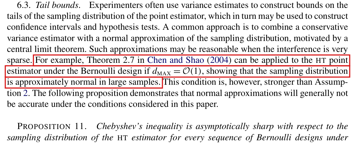
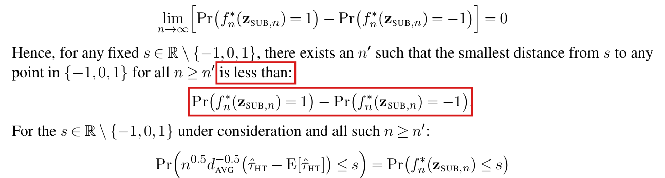
The normal approximation for the HT estimator under a Bernoulli design does not follow from dMAX=O(1)d_{\mathrm{MAX}} = \mathcal{O}(1) alone; it holds under the further condition lim inf⁡n→∞nVar⁡(τ^HT)>0\liminf_{n \to \infty} n\operatorname{Var}(\hat\tau_{\mathrm{HT}}) > 0.

Section 6.3, p. 693 (PDF p. 21), first paragraph, sentence beginning “For example, Theorem 2.7 in Chen and Shao (2004)”

See also under Formal statements (Lean): P009-T7, P009-T8

As printed

Such approximations may be reasonable when the interference is very sparse. For example, Theorem 2.7 in Chen and Shao (2004) can be applied to the HT point estimator under the Bernoulli design if dMAX=O(1)d_{\mathrm{MAX}} = \mathcal{O}(1), showing that the sampling distribution is approximately normal in large samples. This condition is, however, stronger than Assumption 2.

The problem

A bound on dMAXd_{\mathrm{MAX}} limits the dependence between the summands of τ^HT\hat\tau_{\mathrm{HT}}, and it says nothing about their variance. Assumption 1 bounds moments from above only. The sequence of samples is arbitrary, and the variance of τ^HT\hat\tau_{\mathrm{HT}} can be carried by a bounded number of units. Then nVar⁡(τ^HT)n\operatorname{Var}(\hat\tau_{\mathrm{HT}}) tends to zero, and the estimator, centred and divided by its standard deviation, need not be close to normal. This standardized sense is the one that the passage needs, since it concerns tail bounds, confidence intervals and tests. Note that the cited theorem is itself stated for centred summands whose sum has variance one.

Evidence an exact counterexample

The evidence is an exact counterexample and a derivation. For each n≥1n \geq 1, let the assignments be independent with probability 1/21/2, and let y1(z)=z1y_1(\mathbf{z}) = z_1 and yi(z)=0y_i(\mathbf{z}) = 0 for i>1i > 1. All outcomes are bounded by one, Assumption 1 holds with k=2k = 2, and dMAX=dAVG=1d_{\mathrm{MAX}} = d_{\mathrm{AVG}} = 1. Assumption 2 holds as well. In this example τEATE=1/n\tau_{\mathrm{EATE}} = 1/n, τ^HT=2Z1/n\hat\tau_{\mathrm{HT}} = 2Z_1/n and Var⁡(τ^HT)=1/n2\operatorname{Var}(\hat\tau_{\mathrm{HT}}) = 1/n^2, and I obtain

τ^HT−τEATEVar⁡(τ^HT)1/2=2Z1−1for every n.\frac{\hat\tau_{\mathrm{HT}} - \tau_{\mathrm{EATE}}}{\operatorname{Var}(\hat\tau_{\mathrm{HT}})^{1/2}} = 2Z_1 - 1 \qquad \text{for every } n.

The standardized estimator takes the values −1-1 and 11 with probability 1/21/2 each. Its distribution function jumps by 1/21/2 at −1-1. This implies that its Kolmogorov distance from any continuous distribution function is at least 1/41/4, and from the standard normal it is 1/2−Φ(−1)≈0.3411/2 - \Phi(-1) \approx 0.341. Here nVar⁡(τ^HT)=1/nn\operatorname{Var}(\hat\tau_{\mathrm{HT}}) = 1/n. Replacing the outcomes of the units i>1i > 1 by yi(z)=zi−1/2y_i(\mathbf{z}) = z_i - 1/2, I obtain τEATE=1\tau_{\mathrm{EATE}} = 1 and the same two-point law. The failure does not come from an estimand that tends to zero. Both examples agree with an enumeration of all assignments in exact arithmetic for n=1,2,3,4,8,10n = 1, 2, 3, 4, 8, 10.

For the corrected statement, suppose that the design is Bernoulli, that dMAX≤Dd_{\mathrm{MAX}} \leq D for all nn, and that Assumption 1 holds. The outcome of unit ii depends on at most DD treatments, and each configuration of these has probability at least k−Dk^{-D} by Assumption 1A. Since E∣Yi∣2≤k2\mathrm{E}|Y_i|^2 \leq k^2 by Assumption 1B, every potential outcome satisfies ∣yi(z)∣≤k1+D/2|y_i(\mathbf{z})| \leq k^{1 + D/2}. I write nτ^HT=∑iTin\hat\tau_{\mathrm{HT}} = \sum_i T_i. The centred summands Ti−E[Ti]T_i - \mathrm{E}[T_i] are uniformly bounded, and their sum is n(τ^HT−τEATE)n(\hat\tau_{\mathrm{HT}} - \tau_{\mathrm{EATE}}). If two sets of units have no pair with dij=1d_{ij} = 1 between them, then their summands depend on disjoint sets of independent treatments. If nVar⁡(τ^HT)≥c>0n\operatorname{Var}(\hat\tau_{\mathrm{HT}}) \geq c > 0 for all large nn, the variance of the sum is at least cncn. Only O(n)\mathcal{O}(n) connected rr-tuples of units contribute to the rrth cumulant of the sum, so for each r≥3r \geq 3 the rrth cumulant of the standardized sum is O(n1−r/2)\mathcal{O}(n^{1 - r/2}) and tends to zero. Its first two cumulants are 00 and 11, and convergence to the standard normal law follows by the method of moments.

What survives

No proposition, simulation or conclusion of the paper uses this remark. Proposition 11 has its own construction in Supplement A, and the consistency results of Section 5 hold in both examples, where the estimation error is 1/n1/n in absolute value. The preceding sentence, that a normal approximation may be reasonable under very sparse interference, stands. The added condition is the non-degeneracy that a central limit theorem ordinarily carries. It is sufficient and not necessary. The corrected statement divides by the true standard deviation, not by an estimate of it.

Corrected

For example, under Assumption 1, a Bernoulli design and dMAX=O(1)d_{\mathrm{MAX}} = \mathcal{O}(1), the HT point estimator centred at τEATE\tau_{\mathrm{EATE}} and divided by its true standard deviation is asymptotically standard normal, provided that lim inf⁡n→∞nVar⁡(τ^HT)>0\liminf_{n \to \infty} n\operatorname{Var}(\hat\tau_{\mathrm{HT}}) > 0:

τ^HT−τEATEVar⁡(τ^HT)1/2⟶dN(0,1).\frac{\hat\tau_{\mathrm{HT}} - \tau_{\mathrm{EATE}}}{\operatorname{Var}(\hat\tau_{\mathrm{HT}})^{1/2}} \overset{d}{\longrightarrow} \mathcal{N}(0, 1).

This condition on dMAXd_{\mathrm{MAX}} is, however, stronger than Assumption 2.

Crop of the first paragraph of Section 6.3, Tail bounds, and the start of Proposition 11. The paragraph reads: Experimenters often use variance estimates to construct bounds on the tails of the sampling distribution of the point estimator, which in turn may be used to construct confidence intervals and hypothesis tests. A common approach is to combine a conservative variance estimator with a normal approximation of the sampling distribution, motivated by a central limit theorem. Such approximations may be reasonable when the interference is very sparse. For example, Theorem 2.7 in Chen and Shao (2004) can be applied to the HT point estimator under the Bernoulli design if d MAX = O(1), showing that the sampling distribution is approximately normal in large samples. This condition is, however, stronger than Assumption 2. The following proposition demonstrates that normal approximations will generally not be accurate under the conditions considered in this paper. A red outline surrounds the sentence that begins For example, Theorem 2.7 in Chen and Shao (2004). Below the paragraph, Proposition 11 begins: Chebyshev's inequality is asymptotically sharp with respect to the sampling distribution of the HT estimator for every sequence of Bernoulli designs under.
Section 6.3, p. 693 (PDF p. 21). The outline marks the sentence that derives a normal approximation from dMAX=O(1)d_{\mathrm{MAX}} = \mathcal{O}(1) alone.

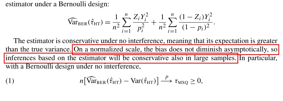
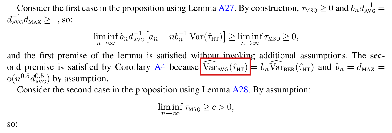
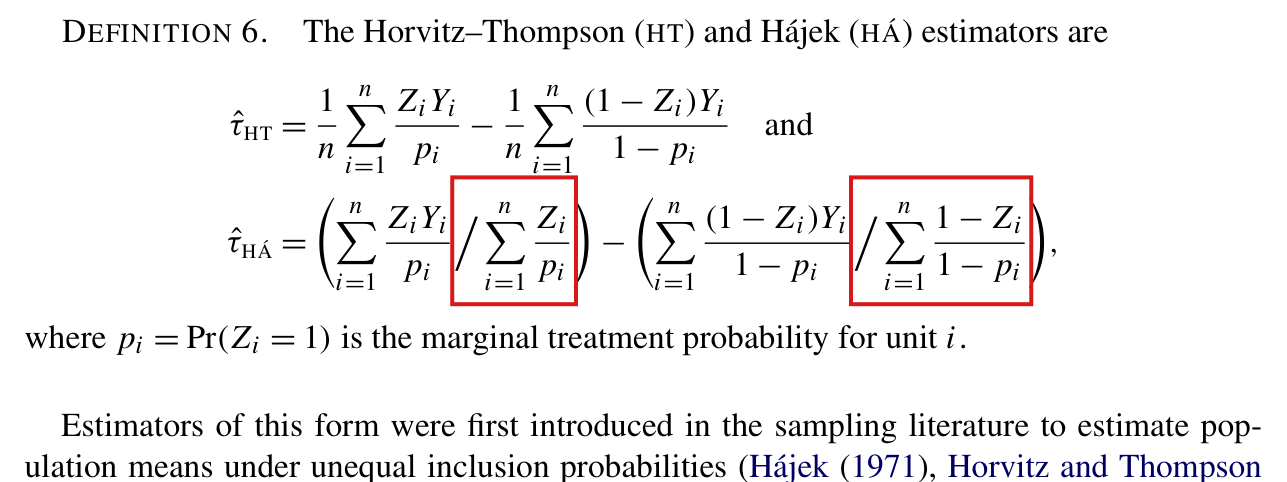
Equation (1) and Definition 10 control the variance estimator on an additive scale, and this property alone does not make inferences based on the estimator conservative in large samples.

Section 6.1, p. 689 (PDF p. 17), second sentence after the display that defines Var⁡^BER(τ^HT)\widehat{\operatorname{Var}}_{\mathrm{BER}}(\hat\tau_{\mathrm{HT}}); see also Definition 10, p. 691 (PDF p. 19)

See also under Formal statements (Lean): P009-T1, P009-T2, P009-T48

As printed

The estimator is conservative under no interference, meaning that its expectation is greater than the true variance. On a normalized scale, the bias does not diminish asymptotically, so inferences based on the estimator will be conservative also in large samples. In particular, with a Bernoulli design under no interference,

(1)n[Var⁡^BER(τ^HT)−Var⁡(τ^HT)]⟶pτMSQ≥0,\text{(1)}\qquad n\bigl[\widehat{\operatorname{Var}}_{\mathrm{BER}}(\hat\tau_{\mathrm{HT}}) - \operatorname{Var}(\hat\tau_{\mathrm{HT}})\bigr] \overset{p}{\longrightarrow} \tau_{\mathrm{MSQ}} \geq 0,
The problem

Equation (1) and Definition 10 both concern the difference between a variance estimator V^\hat V and Var⁡(τ^HT)\operatorname{Var}(\hat\tau_{\mathrm{HT}}) after scaling by nn or by ndAVG−1n d_{\mathrm{AVG}}^{-1}. They say that this scaled difference is not negative in the limit. For a plug-in Chebyshev interval, it is sufficient that V^\hat V is unlikely to be much smaller than Var⁡(τ^HT)\operatorname{Var}(\hat\tau_{\mathrm{HT}}) relative to that variance. The additive property does not provide this when the normalized variance (n/dAVG)Var⁡(τ^HT)(n/d_{\mathrm{AVG}})\operatorname{Var}(\hat\tau_{\mathrm{HT}}) tends to zero. The scaled difference can then vanish while the ratio V^/Var⁡(τ^HT)\hat V/\operatorname{Var}(\hat\tau_{\mathrm{HT}}) is zero with a fixed positive probability. The expectation can equal the true variance when all individual treatment effects are zero. The claim that the scaled bias does not diminish is also too strong. The limit τMSQ\tau_{\mathrm{MSQ}} in (1) depends on nn and may tend to zero, and then the bias on the normalized scale does diminish. The paper prints no interval formula and no coverage theorem. What is affected is this sentence, and any reading of “asymptotically conservative” in Section 6.2 as a guarantee of coverage by itself.

Evidence an exact counterexample

The evidence is an exact counterexample and a derivation. For each n≥1n \geq 1, let Z1,…,ZnZ_1, \dots, Z_n be independent with Pr⁡(Zi=1)=1/2\Pr(Z_i = 1) = 1/2, and let y1(z)=z1y_1(\mathbf{z}) = z_1 and yi(z)=0y_i(\mathbf{z}) = 0 for i≥2i \geq 2. There is no interference, all outcomes lie in [0,1][0, 1], and Assumption 1 holds with k=2k = 2. Further, dAVG=dMAX=λmax⁡=1d_{\mathrm{AVG}} = d_{\mathrm{MAX}} = \lambda_{\max} = 1. Assumption 2 holds, as do the conditions of Proposition 8 and of part A of Propositions 9 and 10. Substituting the outcomes into the definitions of τEATE\tau_{\mathrm{EATE}} and τ^HT\hat\tau_{\mathrm{HT}} and into the display on p. 689, I obtain

τEATE=1n,τ^HT=2Z1n,Var⁡(τ^HT)=1n2,Var⁡^BER(τ^HT)=4Z1n2.\tau_{\mathrm{EATE}} = \frac{1}{n}, \qquad \hat\tau_{\mathrm{HT}} = \frac{2Z_1}{n}, \qquad \operatorname{Var}(\hat\tau_{\mathrm{HT}}) = \frac{1}{n^2}, \qquad \widehat{\operatorname{Var}}_{\mathrm{BER}}(\hat\tau_{\mathrm{HT}}) = \frac{4Z_1}{n^2}.

The expectation of the variance estimator is 2/n22/n^2, which exceeds the variance. Further, τMSQ=1/n\tau_{\mathrm{MSQ}} = 1/n, and n[Var⁡^BER(τ^HT)−Var⁡(τ^HT)]n[\widehat{\operatorname{Var}}_{\mathrm{BER}}(\hat\tau_{\mathrm{HT}}) - \operatorname{Var}(\hat\tau_{\mathrm{HT}})] takes the values −1/n-1/n and 3/n3/n. Equation (1) and Definition 10 therefore hold, and the three inflated estimators of Section 6.2 coincide with Var⁡^BER\widehat{\operatorname{Var}}_{\mathrm{BER}}. The interval τ^HT±(Var⁡^BER(τ^HT)/α)1/2\hat\tau_{\mathrm{HT}} \pm (\widehat{\operatorname{Var}}_{\mathrm{BER}}(\hat\tau_{\mathrm{HT}})/\alpha)^{1/2} with α=1/20\alpha = 1/20 is the plug-in version of the 95% Chebyshev interval that uses the true variance.

The two outcomes of the experiment, each of probability 1/21/2, and the interval with α=1/20\alpha = 1/20.
Eventτ^HT\hat\tau_{\mathrm{HT}}Var⁡^BER(τ^HT)\widehat{\operatorname{Var}}_{\mathrm{BER}}(\hat\tau_{\mathrm{HT}})IntervalContains τEATE=1/n\tau_{\mathrm{EATE}} = 1/n
Z1=0Z_1 = 00000[0,0][0, 0]no
Z1=1Z_1 = 12/n2/n4/n24/n^22/n±80/n2/n \pm \sqrt{80}/nyes

The interval contains τEATE\tau_{\mathrm{EATE}} with probability exactly 1/21/2 for every nn, and the same holds for every α∈(0,1)\alpha \in (0, 1). The interval with the true variance in place of the estimate has half-width 20/n\sqrt{20}/n and always contains τEATE\tau_{\mathrm{EATE}}. In this example (n/dAVG)Var⁡(τ^HT)=1/n(n/d_{\mathrm{AVG}})\operatorname{Var}(\hat\tau_{\mathrm{HT}}) = 1/n tends to zero, and the ratio of the estimate to the variance is 00 or 44. Enumerating all assignments for n=1,…,8n = 1, \dots, 8 in exact arithmetic, I find the same values.

For the corrected statement, let TT be unbiased for θ\theta with variance V>0V > 0, let V^≥0\hat V \geq 0, and fix η∈(0,1)\eta \in (0, 1). On the event V^≥(1−η)V\hat V \geq (1 - \eta)V, the interval T±(V^/α)1/2T \pm (\hat V/\alpha)^{1/2} misses θ\theta only if ∣T−θ∣>((1−η)V/α)1/2|T - \theta| > ((1 - \eta)V/\alpha)^{1/2}. By Chebyshev’s inequality, I have

Pr⁡{∣T−θ∣>(V^/α)1/2}≤Pr⁡{V^<(1−η)V}+α1−η.\Pr\bigl\{|T - \theta| > (\hat V/\alpha)^{1/2}\bigr\} \leq \Pr\bigl\{\hat V < (1 - \eta)V\bigr\} + \frac{\alpha}{1 - \eta}.

If the first term on the right tends to zero for every η\eta, then letting n→∞n \to \infty and afterwards η→0\eta \to 0 shows that the limit inferior of the coverage is at least 1−α1 - \alpha. If (n/dAVG)V≥c>0(n/d_{\mathrm{AVG}})V \geq c > 0 for all large nn, then the event V^<(1−η)V\hat V < (1 - \eta)V is contained in the event ndAVG−1(V^−V)≤−ηcn d_{\mathrm{AVG}}^{-1}(\hat V - V) \leq -\eta c, and Definition 10 implies that the probability of the latter tends to zero.

What survives

Equation (1), Definition 10 and Propositions 8–10 stand as printed. They are statements about the variance estimator, and the example satisfies them. Part B of Propositions 9 and 10 assumes that τMSQ\tau_{\mathrm{MSQ}} is bounded away from zero. In that case, the proofs in Supplement A show that the inflated estimator exceeds the variance with probability tending to one, and this is enough for the coverage statement below. The example does not satisfy part B, and the paragraph after Proposition 9 describes behaviour of this kind. The consistency results of Section 5, Proposition 11 and the simulations are not affected.

Corrected

The estimator is conservative under no interference, meaning that its expectation is at least as large as the true variance. With a Bernoulli design under no interference,

(1)n[Var⁡^BER(τ^HT)−Var⁡(τ^HT)]⟶pτMSQ≥0.\text{(1)}\qquad n\bigl[\widehat{\operatorname{Var}}_{\mathrm{BER}}(\hat\tau_{\mathrm{HT}}) - \operatorname{Var}(\hat\tau_{\mathrm{HT}})\bigr] \overset{p}{\longrightarrow} \tau_{\mathrm{MSQ}} \geq 0.

Equation (1) gives a nonnegative one-sided error for the variance estimator on the scale nn; the scaled bias τMSQ\tau_{\mathrm{MSQ}} may vanish. This variance property alone does not establish that plug-in confidence intervals are conservative.

A coverage statement needs control of the estimator relative to the variance. Let the design be Bernoulli, so that τ^HT\hat\tau_{\mathrm{HT}} is unbiased for τEATE\tau_{\mathrm{EATE}}, let V^≥0\hat V \geq 0 be a variance estimator, and suppose that Var⁡(τ^HT)>0\operatorname{Var}(\hat\tau_{\mathrm{HT}}) > 0 and that

Pr⁡{V^<(1−η)Var⁡(τ^HT)}→0for every 0<η<1.\Pr\bigl\{\hat V < (1 - \eta)\operatorname{Var}(\hat\tau_{\mathrm{HT}})\bigr\} \to 0 \qquad \text{for every } 0 < \eta < 1.

Then, for every α∈(0,1)\alpha \in (0, 1),

lim inf⁡n→∞Pr⁡{∣τ^HT−τEATE∣≤(V^/α)1/2}≥1−α.\liminf_{n \to \infty} \Pr\bigl\{|\hat\tau_{\mathrm{HT}} - \tau_{\mathrm{EATE}}| \leq (\hat V/\alpha)^{1/2}\bigr\} \geq 1 - \alpha.

The displayed condition follows from Definition 10 if lim inf⁡n→∞(n/dAVG)Var⁡(τ^HT)>0\liminf_{n \to \infty}(n/d_{\mathrm{AVG}})\operatorname{Var}(\hat\tau_{\mathrm{HT}}) > 0. Definition 10 alone guarantees only a scaled additive variance property.

Crop of the foot of p. 689. The first line reads: estimator under a Bernoulli design. A displayed formula defines the variance estimator Var-hat BER of tau-hat HT as one over n squared times the sum over i of Z i Y i squared over p i squared, plus one over n squared times the sum over i of (1 minus Z i) Y i squared over (1 minus p i) squared. The text below reads: The estimator is conservative under no interference, meaning that its expectation is greater than the true variance. On a normalized scale, the bias does not diminish asymptotically, so inferences based on the estimator will be conservative also in large samples. In particular, with a Bernoulli design under no interference. Equation (1) follows: n times the bracket Var-hat BER of tau-hat HT minus Var of tau-hat HT converges in probability to tau MSQ, which is at least 0. A red outline surrounds the sentence that begins On a normalized scale.
Section 6.1, p. 689 (PDF p. 17). The outline marks the sentence that passes from the bias of the variance estimator to conservative inferences. Equation (1) follows it.

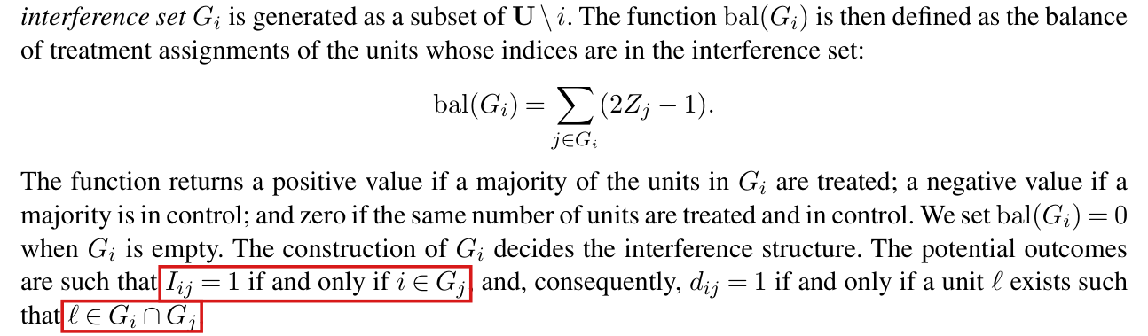
Direct interference from unit ii to unit jj does not imply ξ˘ji≠0\breve\xi_{ji} \neq 0, because the spillover effects under particular assignments can cancel in expectation.

Section 6.1, p. 691 (PDF p. 19), paragraph beginning “Compared to the setting with no interference”, third sentence

See also under Formal statements (Lean): P009-T13, P009-T14

As printed

The term B1B_1 captures the consequences of direct interference between the units. That is, it captures whether unit ii interferes with unit jj directly, in which case ξ˘ji≠0\breve\xi_{ji} \neq 0. If there is no interference, there are no spillover effects, so ξij(1)=ξij(0)=0\xi_{ij}(1) = \xi_{ij}(0) = 0, and B1B_1 is zero.

The problem

Unit ii interferes with unit jj if changing the treatment of ii changes the outcome of jj under at least one assignment (p. 680). The coefficient ξ˘ji\breve\xi_{ji} is an average of such changes over the design (p. 690). Changes that are nonzero under every assignment can have opposite signs and average to zero. Interference from ii to jj therefore does not imply that ξ˘ji\breve\xi_{ji} is nonzero. The converse statement in the next sentence, that without interference B1B_1 is zero, is correct.

Evidence an exact counterexample

The evidence is an exact counterexample. Suppose that three units have independent assignments of probability 1/21/2, and let y2(z)=z1(2z3−1)y_2(\mathbf{z}) = z_1(2z_3 - 1) and y1=y3=0y_1 = y_3 = 0. Since changing z1z_1 changes y2y_2 by 2z3−12z_3 - 1, which is 11 or −1-1, unit 1 interferes with unit 2. For either value of z2z_2, I have ξ21(z2)=E[2Z3−1]=0\xi_{21}(z_2) = \mathrm{E}[2Z_3 - 1] = 0, and hence ξ˘21=0\breve\xi_{21} = 0. All outcomes are bounded by one, and Assumption 1 holds with k=2k = 2. Enumerating the eight assignments in exact arithmetic, I obtain the same values.

What survives

The definitions of ξij(z)\xi_{ij}(z) and ξ˘ij\breve\xi_{ij}, Proposition 7 and the later results on variance estimation are unaffected: the proposition uses the averaged coefficients as defined. Only the explanatory sentence changes.

Corrected

The term B1B_1 captures the contributions of expected direct spillover effects. Direct interference from unit ii to unit jj can give ξ˘ji≠0\breve\xi_{ji} \neq 0, although the spillover effects under particular assignments may average to zero. If there is no interference, there are no spillover effects, so ξij(1)=ξij(0)=0\xi_{ij}(1) = \xi_{ij}(0) = 0, and B1B_1 is zero.

Crop of six lines of text. They read: Compared to the setting with no interference, the limit of the variance estimator contains two additional terms. The term B 1 captures the consequences of direct interference between the units. That is, it captures whether unit i interferes with unit j directly, in which case xi-breve j i is not equal to 0. If there is no interference, there are no spillover effects, so xi i j of 1 = xi i j of 0 = 0, and B 1 is zero. The term B 2 captures the consequences of indirect interference between units, namely when a third unit interferes with both i and j. Red outlines surround the words in which case at the end of the third line and the relation xi-breve j i is not equal to 0 at the start of the fourth.
Section 6.1, p. 691 (PDF p. 19). The outlines mark the words “in which case” and the relation ξ˘ji≠0\breve\xi_{ji} \neq 0 that continues them on the next line.

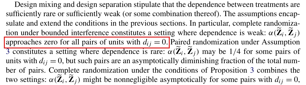
Under complete randomization with bounded interference, α(Z~i,Z~j)\alpha(\widetilde{\mathbf{Z}}_i,\widetilde{\mathbf{Z}}_j) approaches zero for all but a vanishing fraction of the pairs of units with dij=0d_{ij}=0, not for all of them; a fixed pair can keep the value 1/41/4.

Section 5.3, p. 688 (PDF p. 16), first paragraph, sentence beginning “In particular, complete randomization under bounded interference”

See also under Formal statements (Lean): P009-T9, P009-T10

As printed

“In particular, complete randomization under bounded interference constitutes a setting where dependence is weak: α(Z~i,Z~j)\alpha(\widetilde{\mathbf{Z}}_i,\widetilde{\mathbf{Z}}_j) approaches zero for all pairs of units with dij=0d_{ij}=0.”

Later in the same paragraph: “Complete randomization under the conditions of Proposition 3 combines the two settings: α(Z~i,Z~j)\alpha(\widetilde{\mathbf{Z}}_i,\widetilde{\mathbf{Z}}_j) might be nonnegligible asymptotically for some pairs with dij=0d_{ij}=0, but such pairs are rare. For all other pairs with dij=0d_{ij}=0, the pair-level mixing coefficient quickly approaches zero.”

The problem

Corollary 1 on p. 685 defines bounded interference as dAVG=O(1)d_{\mathrm{AVG}}=\mathcal{O}(1), which bounds an average. Such a bound allows a few units that are each affected by a large share of the sample, and under complete randomization the numbers of treated units in two large disjoint sets remain dependent. The sentence claims too much: the mixing coefficient need not approach zero for every pair of units with dij=0d_{ij}=0. It does approach zero, uniformly, outside a set of pairs whose share tends to zero. The paper describes this situation later in the same paragraph, for the conditions of Proposition 3, and the same description applies under bounded interference. The error is in this explanatory sentence only.

Evidence an exact counterexample

The evidence is an exact counterexample for an infinite family of sample sizes and a derivation of the corrected statement.

For the counterexample, let r≥1r\ge1, n=4r+2n=4r+2 and h=n/2h=n/2, so that hh is odd, and let the design be complete randomization with hh treated units. Let the units be divided into two blocks AA and BB of hh units each such that 1∈A1\in A and 2∈B2\in B, and let

y1(z)=1h∑ℓ∈Azℓ,y2(z)=1h∑ℓ∈Bzℓ,yj(z)=zj(3≤j≤n).y_1(\mathbf{z})=\frac{1}{h}\sum_{\ell\in A}z_\ell,\qquad y_2(\mathbf{z})=\frac{1}{h}\sum_{\ell\in B}z_\ell,\qquad y_j(\mathbf{z})=z_j\quad(3\le j\le n).

The potential outcomes lie in [0,1][0,1]. Unit 1 is affected by the treatments in AA, unit 2 by those in BB, and every other unit by its own treatment only. Then d12=0d_{12}=0, dAVG=3−4/nd_{\mathrm{AVG}}=3-4/n and C1=2−2/nC_1=2-2/n, and no unit interferes with more than two units, itself included. Let TAT_A and TB=h−TAT_B=h-T_A be the numbers of treated units in the two blocks. The event {TA≥(h+1)/2}\{T_A\ge(h+1)/2\} is determined by Z~1\widetilde{\mathbf{Z}}_1, the event {TB≤(h−1)/2}\{T_B\le(h-1)/2\} is determined by Z~2\widetilde{\mathbf{Z}}_2, and the two events coincide. Since the map z↦1−z\mathbf{z}\mapsto\mathbf{1}-\mathbf{z} preserves the design and hh is odd, their common probability is 1/21/2. By the definition of the mixing coefficient, I have

α(Z~1,Z~2)≥∣12−12⋅12∣=14,\alpha(\widetilde{\mathbf{Z}}_1,\widetilde{\mathbf{Z}}_2)\ge\Bigl|\frac12-\frac12\cdot\frac12\Bigr|=\frac14 ,

which is the maximum value of the coefficient (p. 687). An enumeration of all assignments for n=6,10,14,18n=6,10,14,18 in exact arithmetic agrees with these values.

For the corrected statement, suppose that dAVG≤Dd_{\mathrm{AVG}}\le D for all large nn, and let ai=∑ℓ=1nIℓia_i=\sum_{\ell=1}^nI_{\ell i} be the number of units that interfere with unit ii. Then ∑i=1nai=nC1≤ndAVG≤nD\sum_{i=1}^na_i=nC_1\le nd_{\mathrm{AVG}}\le nD. Let tn=⌊n1/4⌋t_n=\lfloor n^{1/4}\rfloor. At most nD/tnnD/t_n units have ai>tna_i>t_n, and at most 2Dn2/tn2Dn^2/t_n ordered pairs contain such a unit. Since there are at least n2−nDn^2-nD pairs such that dij=0d_{ij}=0, the excluded share tends to zero. For every other pair such that dij=0d_{ij}=0, the two sets of interfering units are disjoint and have K≤2tnK\le2t_n elements together. A coupling of KK draws without replacement with KK independent draws shows that the two laws of these KK treatments differ by at most εK=K(K−1)/{2(n−K+1)}\varepsilon_K=K(K-1)/\{2(n-K+1)\} on every event. Under the independent law, events on the two sets are independent, and I have

α(Z~i,Z~j)≤3εK≤3(2tn)(2tn−1)2(n−2tn+1)=O(n−1/2)\alpha(\widetilde{\mathbf{Z}}_i,\widetilde{\mathbf{Z}}_j)\le3\varepsilon_K\le\frac{3(2t_n)(2t_n-1)}{2(n-2t_n+1)}=\mathcal{O}(n^{-1/2})

uniformly over these pairs.

What survives

Proposition 3, Corollary 1 and Proposition 5 do not use the sentence. The proof of Proposition 3 treats separately the pairs whose sets of interfering units are large, Corollary 1 follows from Proposition 3 and C1≤dAVGC_1\le d_{\mathrm{AVG}}, and Proposition 5 assumes the averaged conditions of Assumptions 5 and 6. In the counterexample, both estimators are within 6/n6/n of EATE on every assignment, so the example does not contradict root-nn consistency. The correction weakens only the explanatory statement about pairs. The statement for all pairs would hold under a uniform bound on the number of units that interfere with each unit, which is an additional assumption; a bound on the number of units that each unit interferes with is not enough, as the counterexample shows.

Corrected

“In particular, complete randomization under bounded interference constitutes a setting where dependence is weak for most pairs: α(Z~i,Z~j)\alpha(\widetilde{\mathbf{Z}}_i,\widetilde{\mathbf{Z}}_j) approaches zero uniformly for all but an asymptotically vanishing fraction of the pairs of units with dij=0d_{ij}=0; the exceptional pairs can retain nonvanishing dependence.”

In precise form: suppose that the design is complete randomization and that dAVG≤Dd_{\mathrm{AVG}}\le D for all large nn, and let tn=⌊n1/4⌋t_n=\lfloor n^{1/4}\rfloor. Then, for all sufficiently large nn, all pairs of units with dij=0d_{ij}=0, except a share of at most 2Dn/{tn(n−D)}2Dn/\{t_n(n-D)\} of them, satisfy

α(Z~i,Z~j)≤3(2tn)(2tn−1)2(n−2tn+1).\alpha(\widetilde{\mathbf{Z}}_i,\widetilde{\mathbf{Z}}_j)\le\frac{3(2t_n)(2t_n-1)}{2(n-2t_n+1)} .
Crop of the first nine lines of the page. A red box marks the words 'approaches zero for all pairs of units with d i j equals 0', which end the sentence 'In particular, complete randomization under bounded interference constitutes a setting where dependence is weak'.
Section 5.3, p. 688 (PDF p. 16), first paragraph. The marked words state that the coefficient approaches zero for all pairs of units with dij=0d_{ij}=0.

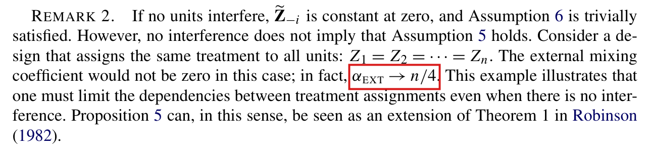
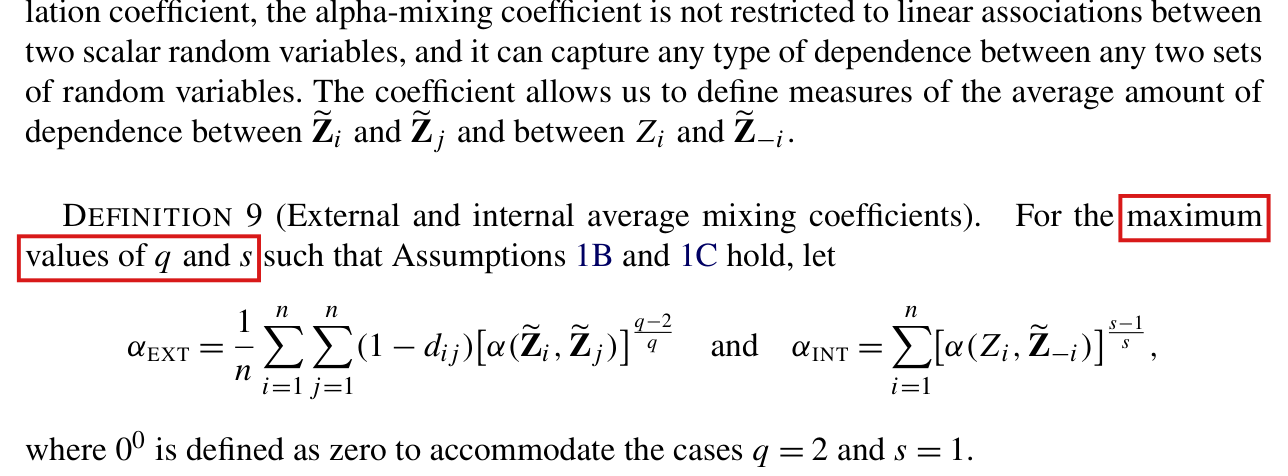
In Remark 2, the external mixing coefficient of the design that assigns the same treatment to all units is (n−1)p(1−p)(n-1)p(1-p), where pp is the probability of treatment; it is asymptotically n/4n/4 only when p=1/2p=1/2.

Remark 2, p. 688 (PDF p. 16), third and fourth sentences

See also under Formal statements (Lean): P009-T26

As printed

“Consider a design that assigns the same treatment to all units: Z1=Z2=⋯=ZnZ_1=Z_2=\cdots=Z_n. The external mixing coefficient would not be zero in this case; in fact, αEXT→n/4\colorbox{#ffe58a}{$\alpha_{\mathrm{EXT}}\to n/4$}.”

The problem

The remark does not state the probability pp with which the common treatment is assigned, and the constant 1/41/4 is correct only for p=1/2p=1/2. In general the coefficient is (n−1)p(1−p)(n-1)p(1-p). The arrow to a quantity that depends on nn is also informal; asymptotic equivalence is meant. The point of the remark is unaffected. Since Assumption 1A keeps pp away from 00 and 11, the coefficient αEXT\alpha_{\mathrm{EXT}} is of order nn and Assumption 5 fails.

Evidence a derivation

The evidence is a derivation from Definition 9. If no units interfere, then dij=0d_{ij}=0 for i≠ji\ne j, and Z~i\widetilde{\mathbf{Z}}_i generates the same events as ZiZ_i. Let Zi=TZ_i=T for all ii, where Pr⁡(T=1)=p\Pr(T=1)=p. The only events are the empty event, {T=0}\{T=0\}, {T=1}\{T=1\} and the whole space. Enumerating the pairs of events, I find α(Zi,Zj)=p−p2=p(1−p)\alpha(Z_i,Z_j)=p-p^2=p(1-p) for i≠ji\ne j. With no interference, each unit has two potential outcomes, and Assumptions 1A and 1B imply that k−1∣yi(z)∣2≤E[∣Yi∣2]≤k2k^{-1}|y_i(z)|^2\le\mathbb{E}[|Y_i|^2]\le k^2. The outcomes are bounded by k3/2k^{3/2}, and with this constant in place of kk, Assumption 1B holds for every qq. The maximum qq of Definition 9 is then infinite, and the exponent (q−2)/q(q-2)/q is 11 (see P009-E006). Summing over the n(n−1)n(n-1) ordered pairs and dividing by nn, I obtain αEXT=(n−1)p(1−p)\alpha_{\mathrm{EXT}}=(n-1)p(1-p). For p=1/3p=1/3 this is 2(n−1)/92(n-1)/9, and for p=1/2p=1/2 it is (n−1)/4(n-1)/4.

What survives

The order nn of the coefficient, the failure of Assumption 5 in this example for every pp that Assumption 1A allows, and Proposition 5 are unaffected. Only the constant changes.

Corrected

“Consider a design that assigns the same treatment to all units, with probability pp of treatment: Z1=Z2=⋯=ZnZ_1=Z_2=\cdots=Z_n. The external mixing coefficient would not be zero in this case; in fact, αEXT=(n−1)p(1−p)\colorbox{#ffe58a}{$\alpha_{\mathrm{EXT}}=(n-1)p(1-p)$}, which is of order nn; for p=1/2p=1/2, αEXT∼n/4\alpha_{\mathrm{EXT}}\sim n/4.”

The statement holds when no units interfere and Assumption 1 holds, with αEXT\alpha_{\mathrm{EXT}} as in Definition 9.

Crop of Remark 2. A red box marks the formula 'alpha EXT tends to n over 4' in the sentence 'The external mixing coefficient would not be zero in this case; in fact, alpha EXT tends to n over 4'.
Remark 2, p. 688 (PDF p. 16). The marked statement gives the external mixing coefficient as tending to n/4n/4.

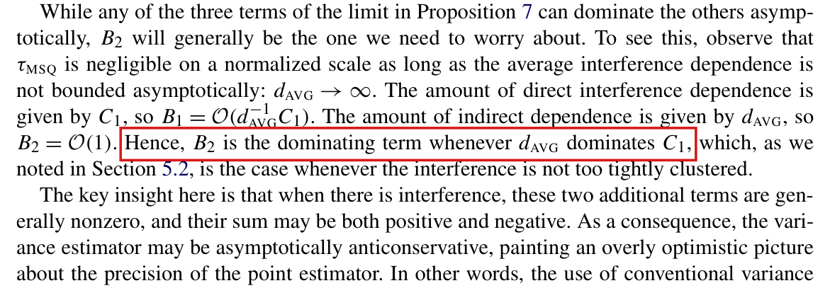
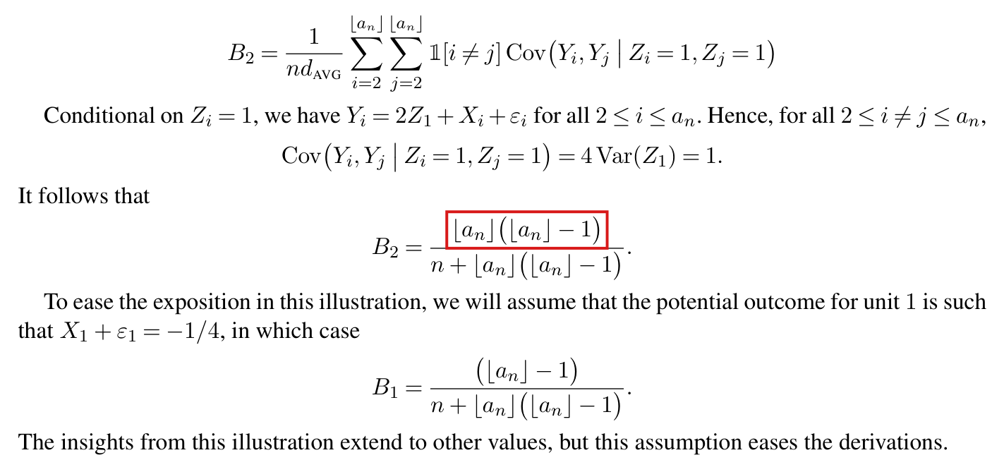
When dAVGd_{\mathrm{AVG}} dominates C1C_1, the term B2B_2 may dominate but need not: the orders B1=O(dAVG−1C1)B_1 = \mathcal{O}(d_{\mathrm{AVG}}^{-1}C_1) and B2=O(1)B_2 = \mathcal{O}(1) are upper bounds, and B2B_2 can be zero.

Section 6.1, p. 691 (PDF p. 19), paragraph beginning “While any of the three terms”, last sentence

See also under Formal statements (Lean): P009-T11, P009-T12

As printed

The amount of direct interference dependence is given by C1C_1, so B1=O(dAVG−1C1)B_1 = \mathcal{O}(d_{\mathrm{AVG}}^{-1}C_1). The amount of indirect dependence is given by dAVGd_{\mathrm{AVG}}, so B2=O(1)B_2 = \mathcal{O}(1). Hence, B2B_2 is the dominating term whenever dAVGd_{\mathrm{AVG}} dominates C1C_1, which, as we noted in Section 5.2, is the case whenever the interference is not too tightly clustered.

The problem

The two orders in the passage are upper bounds. They show that τMSQ/dAVG\tau_{\mathrm{MSQ}}/d_{\mathrm{AVG}} and B1B_1 become small when dAVG/C1d_{\mathrm{AVG}}/C_1 tends to infinity, and they show nothing about how large B2B_2 is. The term B2B_2 is a signed sum of conditional covariances, and its contributions can cancel. Without a lower bound on ∣B2∣|B_2| the conclusion that B2B_2 is the dominating term does not follow. It fails in the example below, where B2=0B_2 = 0 while the other two terms of the limit in Proposition 7 are positive.

Evidence an exact counterexample

The evidence is an exact counterexample. For n=m2n = m^2 with m≥2m \geq 2, I split the units into mm blocks of mm units and label the units of a block 0,1,…,m−10, 1, \dots, m - 1. All assignments are independent with probability 1/21/2, and within each block

y0(z)=z0+z1,yi(z)=zi+z0(1≤i≤m−1).y_0(\mathbf{z}) = z_0 + z_1, \qquad y_i(\mathbf{z}) = z_i + z_0 \quad (1 \leq i \leq m - 1).

All outcomes lie in [0,2][0, 2], and Assumption 1 holds with k=2k = 2 and q=4q = 4. Unit 0 of a block interferes with every unit of the block, unit 1 with itself and unit 0, and each other unit only with itself. Counting these, I find C1=2C_1 = 2. Since every pair of units in a block is affected by the treatment of unit 0, I have dAVG=m=n1/2d_{\mathrm{AVG}} = m = n^{1/2}. In particular, dAVG/C1d_{\mathrm{AVG}}/C_1 tends to infinity and Assumption 2 holds.

Every effect of a unit’s own treatment equals one, and τMSQ=1\tau_{\mathrm{MSQ}} = 1. The spillover effects do not depend on the unit’s own treatment, which implies that ξij(1)−ξij(0)=0\xi_{ij}(1) - \xi_{ij}(0) = 0. The product ξ˘ijξ˘ji\breve\xi_{ij}\breve\xi_{ji} is nonzero only for the two ordered pairs formed by units 0 and 1 of a block, where it equals one. Summing over the blocks, I find B1=2m/(ndAVG)=2/m2B_1 = 2m/(n d_{\mathrm{AVG}}) = 2/m^2. Each outcome is a sum of treatments, yi(z)=∑kAikzky_i(\mathbf{z}) = \sum_k A_{ik}z_k with Aik∈{0,1}A_{ik} \in \{0, 1\}. For i≠ji \neq j, I have

Cov⁡(Yi,Yj∣Zi=a,Zj=b)=14∑k∉{i,j}AikAjk,\operatorname{Cov}(Y_i, Y_j \mid Z_i = a, Z_j = b) = \frac{1}{4}\sum_{k \notin \{i, j\}} A_{ik}A_{jk},

which does not depend on aa or bb. The alternating sum over aa and bb in the definition of B2B_2 is therefore zero for every pair, and B2=0B_2 = 0. Note that the covariances themselves are not all zero.

The terms of the limit in Proposition 7 in the example, for n=m2n = m^2 and m=2,…,8m = 2, \dots, 8.
nnC1C_1dAVGd_{\mathrm{AVG}}τMSQ/dAVG\tau_{\mathrm{MSQ}}/d_{\mathrm{AVG}}B1B_1B2B_2
4422221/21/21/21/200
9922331/31/32/92/900
161622441/41/41/81/800
252522551/51/52/252/2500
363622661/61/61/181/1800
494922771/71/72/492/4900
646422881/81/81/321/3200

For m≥3m \geq 3 the largest of the three terms is τMSQ/dAVG=n−1/2\tau_{\mathrm{MSQ}}/d_{\mathrm{AVG}} = n^{-1/2}, and B2B_2 is zero for every mm. I enumerated in exact arithmetic all assignments of a block of up to eight units, and of the whole sample for n=9n = 9 and for n=10n = 10 (with one isolated unit). The results agree with these values and with the identity of Proposition 7 for the expected bias. A sample of any size nn can be built in the same way from blocks of ⌊n1/2⌋\lfloor n^{1/2} \rfloor units and isolated units.

What survives

Proposition 7 and the two upper bounds are correct as printed, and no later result uses the comparison: Propositions 8–10 rest on variance bounds and concentration. The warning that the conventional variance estimator may be anticonservative under interference stands. What changes is that B2B_2 is the term that may be of order one, not the term that must be largest.

Corrected

The amount of direct interference dependence is given by C1C_1, so B1=O(dAVG−1C1)B_1 = \mathcal{O}(d_{\mathrm{AVG}}^{-1}C_1). The amount of indirect dependence is given by dAVGd_{\mathrm{AVG}}, so B2=O(1)B_2 = \mathcal{O}(1). Hence, when dAVG/C1d_{\mathrm{AVG}}/C_1 tends to infinity, τMSQ/dAVG\tau_{\mathrm{MSQ}}/d_{\mathrm{AVG}} and B1B_1 vanish on this scale, whereas B2B_2 is O(1)\mathcal{O}(1) and may dominate.

The remark that dAVGd_{\mathrm{AVG}} dominates C1C_1 whenever the interference is not too tightly clustered stays as printed. If guaranteed dominance is wanted, a lower bound on the magnitude of B2B_2 must be assumed: it suffices that ∣B2∣≥c>0|B_2| \geq c > 0 for all large nn, or more generally that C1/(dAVG∣B2∣)→0C_1/(d_{\mathrm{AVG}}|B_2|) \to 0.

Crop of two paragraphs. The first reads: While any of the three terms of the limit in Proposition 7 can dominate the others asymptotically, B 2 will generally be the one we need to worry about. To see this, observe that tau MSQ is negligible on a normalized scale as long as the average interference dependence is not bounded asymptotically: d AVG tends to infinity. The amount of direct interference dependence is given by C 1, so B 1 = O(d AVG to the minus 1 times C 1). The amount of indirect dependence is given by d AVG, so B 2 = O(1). Hence, B 2 is the dominating term whenever d AVG dominates C 1, which, as we noted in Section 5.2, is the case whenever the interference is not too tightly clustered. A red outline surrounds the words Hence, B 2 is the dominating term whenever d AVG dominates C 1. The second paragraph begins: The key insight here is that when there is interference, these two additional terms are generally nonzero, and their sum may be both positive and negative.
Section 6.1, p. 691 (PDF p. 19). The outline marks the clause that draws dominance of B2B_2 from the two upper bounds stated just before it.

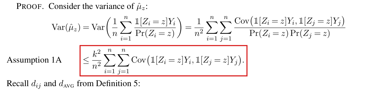
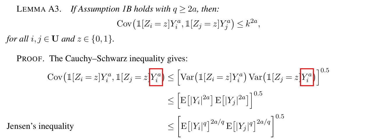
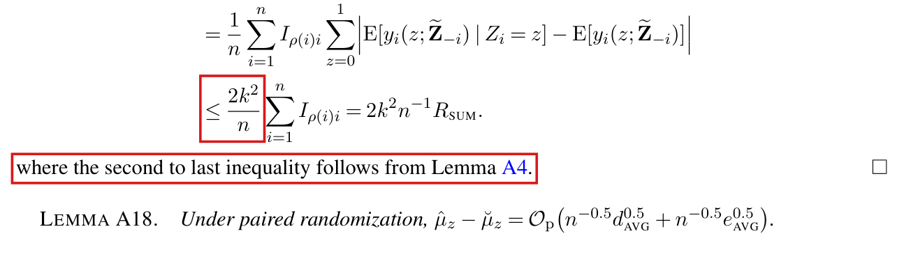
Four proofs in Supplement A bound a weighted sum of signed covariances by replacing each weight with its maximum, which is not a valid inequality; with absolute covariances, and with the diagonal terms kept in Lemma A23, the same final bounds follow.

Supplement A, proof of Lemma A9, p. 8, first display, step labelled “Assumption 1A”; the same step in the proofs of Lemma A22 (p. 22), Lemma A23 (p. 23) and Lemma A25 (p. 25)

See also under Formal statements (Lean): P009-T3, P009-T4, P009-T16, P009-T29, P009-T41, P009-T46, P009-T47

As printed

Proof of Lemma A9, p. 8; the second line is labelled “Assumption 1A”:

Var⁡(μ^z)=Var⁡(1n∑i=1n1[Zi=z]YiPr⁡(Zi=z))=1n2∑i=1n∑j=1nCov⁡(1[Zi=z]Yi,1[Zj=z]Yj)Pr⁡(Zi=z)Pr⁡(Zj=z)≤k2n2∑i=1n∑j=1nCov⁡(1[Zi=z]Yi,1[Zj=z]Yj).\begin{aligned} \operatorname{Var}(\hat\mu_z)&=\operatorname{Var}\bigg(\frac1n\sum_{i=1}^n\frac{\mathbf{1}[Z_i=z]Y_i}{\Pr(Z_i=z)}\bigg)=\frac1{n^2}\sum_{i=1}^n\sum_{j=1}^n\frac{\operatorname{Cov}\big(\mathbf{1}[Z_i=z]Y_i,\mathbf{1}[Z_j=z]Y_j\big)}{\Pr(Z_i=z)\Pr(Z_j=z)}\\ &\le\frac{k^2}{n^2}\sum_{i=1}^n\sum_{j=1}^n\colorbox{#ffe58a}{$\displaystyle \operatorname{Cov}\big(\mathbf{1}[Z_i=z]Y_i,\mathbf{1}[Z_j=z]Y_j\big)$}. \end{aligned}

Proof of Lemma A22, p. 22: “Assumption 1A gives:”

Var⁡(μ^z)=Var⁡(1n∑i=1n1[Zi=z]YiPr⁡(Zi=z))≤k2n2∑i=1n∑j=1nCov⁡(1[Zi=z]Yi,1[Zj=z]Yj)\operatorname{Var}(\hat\mu_z)=\operatorname{Var}\bigg(\frac1n\sum_{i=1}^n\frac{\mathbf{1}[Z_i=z]Y_i}{\Pr(Z_i=z)}\bigg)\le\frac{k^2}{n^2}\sum_{i=1}^n\sum_{j=1}^n\colorbox{#ffe58a}{$\displaystyle \operatorname{Cov}\big(\mathbf{1}[Z_i=z]Y_i,\mathbf{1}[Z_j=z]Y_j\big)$}

Proof of Lemma A23, p. 23: “First, consider the variance of n^z/n\hat n_z/n. Assumption 1A gives:”

Var⁡(n^z/n)=Var⁡(1n∑i=1n1[Zi=z]Pr⁡(Zi=z))≤k2n2∑i=1n∑j=1nCov⁡(1[Zi=z],1[Zj=z])=k2n2∑i=1n∑j=1n[Pr⁡(Zi=z,Zj=z)−Pr⁡(Zi=z)Pr⁡(Zj=z)]≤k2n2∑i=1n∑j≠iα(Zi,Zj)≤k2dAVGn+k2n2∑i=1n∑j=1n(1−dij)α(Zi,Zj),\begin{aligned} \operatorname{Var}(\hat n_z/n)&=\operatorname{Var}\bigg(\frac1n\sum_{i=1}^n\frac{\mathbf{1}[Z_i=z]}{\Pr(Z_i=z)}\bigg)\le\frac{k^2}{n^2}\sum_{i=1}^n\sum_{j=1}^n\colorbox{#ffe58a}{$\displaystyle \operatorname{Cov}\big(\mathbf{1}[Z_i=z],\mathbf{1}[Z_j=z]\big)$}\\ &=\frac{k^2}{n^2}\sum_{i=1}^n\sum_{j=1}^n\Big[\Pr(Z_i=z,Z_j=z)-\Pr(Z_i=z)\Pr(Z_j=z)\Big]\\ &\le\frac{k^2}{n^2}\sum_{i=1}^n\sum_{\colorbox{#ffe58a}{$\displaystyle j\ne i$}}\alpha\big(Z_i,Z_j\big)\le\frac{k^2d_{\mathrm{AVG}}}{n}+\frac{k^2}{n^2}\sum_{i=1}^n\sum_{j=1}^n(1-d_{ij})\alpha\big(Z_i,Z_j\big), \end{aligned}

Proof of Lemma A25, p. 25: “Given Assumption 1A, for z∈{0,1}z\in\{0,1\}:”

Var⁡(∑i=1n1[Zi=z]Yi2[Pr⁡(Zi=z)]2)≤k4∑i=1n∑j=1nCov⁡(1[Zi=z]Yi2,1[Zj=z]Yj2).\operatorname{Var}\bigg(\sum_{i=1}^n\frac{\mathbf{1}[Z_i=z]Y_i^2}{[\Pr(Z_i=z)]^2}\bigg)\le k^4\sum_{i=1}^n\sum_{j=1}^n\colorbox{#ffe58a}{$\displaystyle \operatorname{Cov}\big(\mathbf{1}[Z_i=z]Y_i^2,\mathbf{1}[Z_j=z]Y_j^2\big)$}.
The problem

By Assumption 1A, each weight 1/[Pr⁡(Zi=z)Pr⁡(Zj=z)]1/[\Pr(Z_i=z)\Pr(Z_j=z)] lies between 11 and k2k^2. When the treatment probabilities differ across units the weights differ across pairs, and the covariances can be negative. Replacing every weight by k2k^2 then does not give an upper bound: in the unweighted sum, a negative covariance that carries a small weight can cancel a positive covariance that carries a large one. The proof of Lemma A23 applies the same step to the indicators 1[Zi=z]\mathbf{1}[Z_i=z], and the proof of Lemma A25 applies it to the squared outcomes, with weights at most k4k^4. The third line in the proof of Lemma A23 also sums over j≠ij\ne i, which leaves out the variances of the indicators; that index is the subject of P009-E010. The step is valid in the proofs of Lemmas A15 and A18. There every unit has the same treatment probability, and the weight is a common factor of a sum that is itself a variance.

Evidence an exact counterexample

The evidence is three exact counterexamples with two units and a derivation of the repaired bounds. In each example z=1z=1, k=4k=4, the treatment probabilities of the two units are 1/41/4 and 3/43/4, and every potential outcome is at most one in absolute value.

  • Lemmas A9 and A22. Let Z1Z_1 and Z2Z_2 be independent, and let y1(z)=z2y_1(\mathbf{z})=z_2 and y2(z)=−z1y_2(\mathbf{z})=-z_1. Then 1[Z1=1]Y1=Z1Z2=−1[Z2=1]Y2\mathbf{1}[Z_1=1]Y_1=Z_1Z_2=-\mathbf{1}[Z_2=1]Y_2. The four covariances sum to zero, and μ^1=(4/3)Z1Z2\hat\mu_1=(4/3)Z_1Z_2 has variance 13/4813/48.
  • Lemma A23. Let Pr⁡(Z=(1,0))=1/4\Pr(\mathbf{Z}=(1,0))=1/4 and Pr⁡(Z=(0,1))=3/4\Pr(\mathbf{Z}=(0,1))=3/4, and let all potential outcomes equal one. Then Z1+Z2=1Z_1+Z_2=1, the covariances of the indicators sum to zero, and n^1/n\hat n_1/n takes the values 22 and 2/32/3 and has variance 1/31/3.
  • Lemma A25. Let Z1Z_1 and Z2Z_2 be independent, and let y1(z)=1y_1(\mathbf{z})=1 and y2(z)=1−z1y_2(\mathbf{z})=1-z_1. The covariances sum to 39/25639/256. The printed bound is then 3939, and the variance on the left is 367/9367/9.
The left side of each printed inequality in the two-unit examples, the printed bound, and the bound with absolute covariances.
ProofVariancePrinted boundBound with absolute covariances
Lemmas A9 and A2213/4813/480039/1639/16
Lemma A231/31/30033
Lemma A25367/9367/93939183183

The failure is not special to n=2n=2. With mm independent copies of an example and n=2mn=2m, the three variances are 13/(48m)13/(48m), 1/(3m)1/(3m) and 367m/9367m/9, the printed bounds are 00, 00 and 39m39m, and dAVG≤2d_{\mathrm{AVG}}\le2 and αEXT≤1\alpha_{\mathrm{EXT}}\le1.

The repair rests on the following inequality. For random variables X1,…,XnX_1,\dots,X_n with finite variances and constants 0<wi≤K0<w_i\le K, I have

Var⁡(∑i=1nwiXi)=∑i=1n∑j=1nwiwjCov⁡(Xi,Xj)≤K2∑i=1n∑j=1n∣Cov⁡(Xi,Xj)∣.\operatorname{Var}\Big(\sum_{i=1}^nw_iX_i\Big)=\sum_{i=1}^n\sum_{j=1}^nw_iw_j\operatorname{Cov}(X_i,X_j)\le K^2\sum_{i=1}^n\sum_{j=1}^n\big|\operatorname{Cov}(X_i,X_j)\big|.

The later steps of the four proofs also hold with absolute covariances. By the Cauchy–Schwarz argument in the proof of Lemma A3, I have ∣Cov⁡(1[Zi=z]Yia,1[Zj=z]Yja)∣≤k2a|\operatorname{Cov}(\mathbf{1}[Z_i=z]Y_i^a,\mathbf{1}[Z_j=z]Y_j^a)|\le k^{2a} for q≥2aq\ge2a. Under a Bernoulli design the covariance is zero when dij=0d_{ij}=0. Lemma A21 is stated for the absolute covariance. Finally, ∣Cov⁡(1[Zi=z],1[Zj=z])∣≤α(Zi,Zj)≤1/4|\operatorname{Cov}(\mathbf{1}[Z_i=z],\mathbf{1}[Z_j=z])|\le\alpha(Z_i,Z_j)\le1/4 for every pair, including i=ji=j.

What survives

The final bounds of the four lemmas hold under the same assumptions and with the same constants: k4n−1dAVGk^4n^{-1}d_{\mathrm{AVG}} in Lemma A9, k4n−1dAVG+10k4n−1αEXTk^4n^{-1}d_{\mathrm{AVG}}+10k^4n^{-1}\alpha_{\mathrm{EXT}} in Lemma A22, k2n−1dAVG+k2n−1αEXTk^2n^{-1}d_{\mathrm{AVG}}+k^2n^{-1}\alpha_{\mathrm{EXT}} for Var⁡(n^z/n)\operatorname{Var}(\hat n_z/n) in Lemma A23, and 4k8n−1dAVG4k^8n^{-1}d_{\mathrm{AVG}} for the variance of the normalized variance estimator in Lemma A25. The results that rest on these lemmas are unchanged: Propositions 2, 5, 6 and 7, Corollaries A3–A5 and, through them, Propositions 8–10. Lemmas A15 and A18 need no change. Only the printed derivations change.

Corrected

The first inequality of each proof is replaced as follows, and the later steps are read with absolute covariances.

Lemma A9 (Bernoulli design, Assumption 1):

Var⁡(μ^z)≤k2n2∑i=1n∑j=1n∣Cov⁡(1[Zi=z]Yi,1[Zj=z]Yj)∣=k2n2∑i=1n∑j=1ndij∣Cov⁡(1[Zi=z]Yi,1[Zj=z]Yj)∣≤k4n−1dAVG.\begin{aligned} \operatorname{Var}(\hat\mu_z)&\le\frac{k^2}{n^2}\sum_{i=1}^n\sum_{j=1}^n\colorbox{#ffe58a}{$\displaystyle \big|\operatorname{Cov}\big(\mathbf{1}[Z_i=z]Y_i,\mathbf{1}[Z_j=z]Y_j\big)\big|$}\\ &=\frac{k^2}{n^2}\sum_{i=1}^n\sum_{j=1}^nd_{ij}\big|\operatorname{Cov}\big(\mathbf{1}[Z_i=z]Y_i,\mathbf{1}[Z_j=z]Y_j\big)\big|\le k^4n^{-1}d_{\mathrm{AVG}}. \end{aligned}

Lemma A22 (arbitrary designs, Assumption 1, with qq the maximum value that satisfies Assumption 1B):

Var⁡(μ^z)≤k2n2∑i=1n∑j=1n∣Cov⁡(1[Zi=z]Yi,1[Zj=z]Yj)∣≤k4n−1dAVG+10k4n2∑i=1n∑j=1n(1−dij) α(Z~i,Z~j)q−2q=k4n−1dAVG+10k4n−1αEXT.\begin{aligned} \operatorname{Var}(\hat\mu_z)&\le\frac{k^2}{n^2}\sum_{i=1}^n\sum_{j=1}^n\colorbox{#ffe58a}{$\displaystyle \big|\operatorname{Cov}\big(\mathbf{1}[Z_i=z]Y_i,\mathbf{1}[Z_j=z]Y_j\big)\big|$}\\ &\le k^4n^{-1}d_{\mathrm{AVG}}+\frac{10k^4}{n^2}\sum_{i=1}^n\sum_{j=1}^n(1-d_{ij})\,\alpha\big(\widetilde{\mathbf{Z}}_i,\widetilde{\mathbf{Z}}_j\big)^{\frac{q-2}{q}}=k^4n^{-1}d_{\mathrm{AVG}}+10k^4n^{-1}\alpha_{\mathrm{EXT}}. \end{aligned}

Lemma A23 (arbitrary designs, Assumption 1):

Var⁡(n^z/n)≤k2n2∑i=1n∑j=1n∣Cov⁡(1[Zi=z],1[Zj=z])∣≤k2n2∑i=1n∑j=1nα(Zi,Zj)≤k2dAVGn+k2n2∑i=1n∑j=1n(1−dij)α(Zi,Zj).\begin{aligned} \operatorname{Var}(\hat n_z/n)&\le\frac{k^2}{n^2}\sum_{i=1}^n\sum_{j=1}^n\colorbox{#ffe58a}{$\displaystyle \big|\operatorname{Cov}\big(\mathbf{1}[Z_i=z],\mathbf{1}[Z_j=z]\big)\big|$}\\ &\le\frac{k^2}{n^2}\sum_{i=1}^n\sum_{\colorbox{#ffe58a}{$\displaystyle j=1$}}^n\alpha\big(Z_i,Z_j\big)\le\frac{k^2d_{\mathrm{AVG}}}{n}+\frac{k^2}{n^2}\sum_{i=1}^n\sum_{j=1}^n(1-d_{ij})\alpha\big(Z_i,Z_j\big). \end{aligned}

The diagonal terms have dii=1d_{ii}=1 and are covered by the term k2dAVG/nk^2d_{\mathrm{AVG}}/n, since α(Zi,Zj)≤1/4\alpha(Z_i,Z_j)\le1/4.

Lemma A25 (Bernoulli design, Assumption 1 with q≥4q\ge4), for z∈{0,1}z\in\{0,1\}:

Var⁡(∑i=1n1[Zi=z]Yi2[Pr⁡(Zi=z)]2)≤k4∑i=1n∑j=1n∣Cov⁡(1[Zi=z]Yi2,1[Zj=z]Yj2)∣=k4∑i=1n∑j=1ndij∣Cov⁡(1[Zi=z]Yi2,1[Zj=z]Yj2)∣≤k8ndAVG.\begin{aligned} \operatorname{Var}\bigg(\sum_{i=1}^n\frac{\mathbf{1}[Z_i=z]Y_i^2}{[\Pr(Z_i=z)]^2}\bigg)&\le k^4\sum_{i=1}^n\sum_{j=1}^n\colorbox{#ffe58a}{$\displaystyle \big|\operatorname{Cov}\big(\mathbf{1}[Z_i=z]Y_i^2,\mathbf{1}[Z_j=z]Y_j^2\big)\big|$}\\ &=k^4\sum_{i=1}^n\sum_{j=1}^nd_{ij}\big|\operatorname{Cov}\big(\mathbf{1}[Z_i=z]Y_i^2,\mathbf{1}[Z_j=z]Y_j^2\big)\big|\le k^8nd_{\mathrm{AVG}}. \end{aligned}
Crop of the first display of the proof. The first line writes the variance of mu-hat_z as one over n squared times the double sum of covariances divided by Pr(Z_i = z) Pr(Z_j = z). A red box marks the second line, labelled Assumption 1A: at most k squared over n squared times the double sum of the covariances, without absolute values.
Supplement A, p. 8: the opening of the proof of Lemma A9. The marked line replaces the weights 1/[Pr⁡(Zi=z)Pr⁡(Zj=z)]1/[\Pr(Z_i=z)\Pr(Z_j=z)] by k2k^2 in a sum of signed covariances.
Crop showing Lemma A22 and the line 'Proof. Assumption 1A gives'. A red box marks the right side of the display: at most k squared over n squared times the double sum of the covariances of 1[Z_i = z] Y_i and 1[Z_j = z] Y_j.
Supplement A, p. 22: Lemma A22 and the first line of its proof, with the same step marked.
Crop of a three-line display for the variance of n-hat_z over n. A red box marks the right side of the first line: at most k squared over n squared times the double sum of the covariances of 1[Z_i = z] and 1[Z_j = z]. A second red box marks the start of the third line: k squared over n squared times the sum over i and over j not equal to i of alpha(Z_i, Z_j).
Supplement A, p. 23: the first display of the proof of Lemma A23. The first marked term is the same step for the indicators; the second marked term is the sum over j≠ij\ne i, which leaves out the diagonal terms.
Crop of one display from the proof of Lemma A25. A red box marks its right side: at most k to the fourth times the double sum of the covariances of 1[Z_i = z] Y_i squared and 1[Z_j = z] Y_j squared.
Supplement A, p. 25: the step in the proof of Lemma A25, for squared outcomes and with k4k^4.

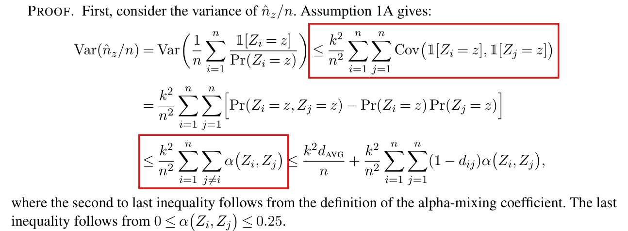
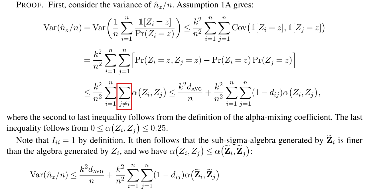
The middle sum in the first display of the proof of Lemma A23 should run over all jj and not over j≠ij \neq i: the terms with j=ij = i are variances of assignment indicators and are positive.

Supplement A, p. 23 (PDF p. 23 of the supplement), proof of Lemma A23, first display, third line

See also under Formal statements (Lean): P009-T4, P009-T15, P009-T16, P009-T46

As printed
=k2n2∑i=1n∑j=1n[Pr⁡(Zi=z,Zj=z)−Pr⁡(Zi=z)Pr⁡(Zj=z)]≤k2n2∑i=1n∑j≠iα(Zi,Zj)≤k2dAVGn+k2n2∑i=1n∑j=1n(1−dij)α(Zi,Zj),\begin{aligned} &= \frac{k^2}{n^2}\sum_{i=1}^n\sum_{j=1}^n \Bigl[\Pr(Z_i = z, Z_j = z) - \Pr(Z_i = z)\Pr(Z_j = z)\Bigr] \\ &\leq \frac{k^2}{n^2}\sum_{i=1}^n \colorbox{#ffe58a}{$\displaystyle \sum_{j \neq i}$} \alpha(Z_i, Z_j) \leq \frac{k^2 d_{\mathrm{AVG}}}{n} + \frac{k^2}{n^2}\sum_{i=1}^n\sum_{j=1}^n (1 - d_{ij})\alpha(Z_i, Z_j), \end{aligned}
The problem

For j=ij = i the bracketed term of the display equals Pr⁡(Zi=z)(1−Pr⁡(Zi=z))\Pr(Z_i = z)(1 - \Pr(Z_i = z)), the variance of the indicator of Zi=zZ_i = z, which is positive under Assumption 1A. The sum of α(Zi,Zj)\alpha(Z_i, Z_j) over j≠ij \neq i does not bound these terms: under independent assignments it is zero, while the left side is positive. The sum over all jj is what the neighbouring expressions use, and the term k2dAVG/nk^2 d_{\mathrm{AVG}}/n of the last expression already covers the pairs j=ij = i, because dii=1d_{ii} = 1. The first inequality of the same display, which passes from the weighted variance to a signed sum of covariances, is the subject of P009-E009.

Evidence an exact counterexample

The evidence is an exact counterexample and a derivation. For each nn, suppose that nn units have independent assignments of probability 1/21/2 and outcomes yi(z)=ziy_i(\mathbf{z}) = z_i, and let k=2k = 2 and z=1z = 1. This sequence satisfies Assumptions 1, 2 and 5. Note that α(Zi,Zj)=0\alpha(Z_i, Z_j) = 0 for j≠ij \neq i and α(Zi,Zi)=1/4\alpha(Z_i, Z_i) = 1/4. The first line of the passage as printed above equals 1/n1/n, which is also the value of Var⁡(n^z/n)\operatorname{Var}(\hat n_z/n), and the printed middle expression is 00. For n=4n = 4 the printed inequality reads 1/4≤01/4 \leq 0. With the sum over all jj the middle expression is 1/41/4, and the last expression is 11.

For the corrected display, the definition of the alpha-mixing coefficient implies that Pr⁡(Zi=z,Zj=z)−Pr⁡(Zi=z)Pr⁡(Zj=z)≤α(Zi,Zj)\Pr(Z_i = z, Z_j = z) - \Pr(Z_i = z)\Pr(Z_j = z) \leq \alpha(Z_i, Z_j) for every pair, including j=ij = i. Summing over all pairs, I obtain the corrected middle expression. Since Iii=1I_{ii} = 1, Definition 5 gives dii=1d_{ii} = 1. Using dij+(1−dij)=1d_{ij} + (1 - d_{ij}) = 1 and 0≤α(Zi,Zj)≤1/40 \leq \alpha(Z_i, Z_j) \leq 1/4, I have

∑i=1n∑j=1nα(Zi,Zj)≤14∑i=1n∑j=1ndij+∑i=1n∑j=1n(1−dij)α(Zi,Zj)=n4dAVG+∑i=1n∑j=1n(1−dij)α(Zi,Zj).\sum_{i=1}^n\sum_{j=1}^n \alpha(Z_i, Z_j) \leq \frac{1}{4}\sum_{i=1}^n\sum_{j=1}^n d_{ij} + \sum_{i=1}^n\sum_{j=1}^n (1 - d_{ij})\alpha(Z_i, Z_j) = \frac{n}{4}d_{\mathrm{AVG}} + \sum_{i=1}^n\sum_{j=1}^n (1 - d_{ij})\alpha(Z_i, Z_j).

Multiplying by k2/n2k^2/n^2 gives a bound that is no larger than the printed last expression.

What survives

The last expression of the display, the bound Var⁡(n^z/n)≤k2n−1(dAVG+αEXT)\operatorname{Var}(\hat n_z/n) \leq k^2 n^{-1}(d_{\mathrm{AVG}} + \alpha_{\mathrm{EXT}}) that follows it, the rate of Lemma A23 and the rates of the Hájek estimator in Propositions 5 and 6 are unchanged. No assumption is added.

Corrected
=k2n2∑i=1n∑j=1n[Pr⁡(Zi=z,Zj=z)−Pr⁡(Zi=z)Pr⁡(Zj=z)]≤k2n2∑i=1n∑j=1nα(Zi,Zj)≤k2dAVGn+k2n2∑i=1n∑j=1n(1−dij)α(Zi,Zj),\begin{aligned} &= \frac{k^2}{n^2}\sum_{i=1}^n\sum_{j=1}^n \Bigl[\Pr(Z_i = z, Z_j = z) - \Pr(Z_i = z)\Pr(Z_j = z)\Bigr] \\ &\leq \frac{k^2}{n^2}\sum_{i=1}^n \colorbox{#ffe58a}{$\displaystyle \sum_{j=1}^n$} \alpha(Z_i, Z_j) \leq \frac{k^2 d_{\mathrm{AVG}}}{n} + \frac{k^2}{n^2}\sum_{i=1}^n\sum_{j=1}^n (1 - d_{ij})\alpha(Z_i, Z_j), \end{aligned}
Crop of the opening of a proof. The first line reads: Proof. First, consider the variance of n-hat z over n. Assumption 1A gives. A display of three lines follows. First line: Var of n-hat z over n equals the variance of one over n times the sum over i of the indicator of Z i = z divided by Pr(Z i = z), which is at most k squared over n squared times the double sum over i and j from 1 to n of the covariance of the indicators of Z i = z and Z j = z. Second line: equals k squared over n squared times the double sum over i and j from 1 to n of Pr(Z i = z, Z j = z) minus Pr(Z i = z) Pr(Z j = z). Third line: is at most k squared over n squared times the sum over i from 1 to n and the sum over j not equal to i of alpha(Z i, Z j), which is at most k squared d AVG over n plus k squared over n squared times the double sum over i and j from 1 to n of (1 minus d i j) alpha(Z i, Z j). A red outline surrounds the summation sign with the index j not equal to i. The text below reads: where the second to last inequality follows from the definition of the alpha-mixing coefficient. The last inequality follows from 0 at most alpha(Z i, Z j) at most 0.25. Note that I i i = 1 by definition. It then follows that the sub-sigma-algebra generated by Z-tilde i is finer than the algebra generated by Z i, and we have alpha(Z i, Z j) at most alpha(Z-tilde i, Z-tilde j). The crop ends with the first line of the next display.
Supplement A, p. 23, first display of the proof of Lemma A23. The outline marks the sum over j≠ij \neq i in the third line; the sums before and after it run over all jj.

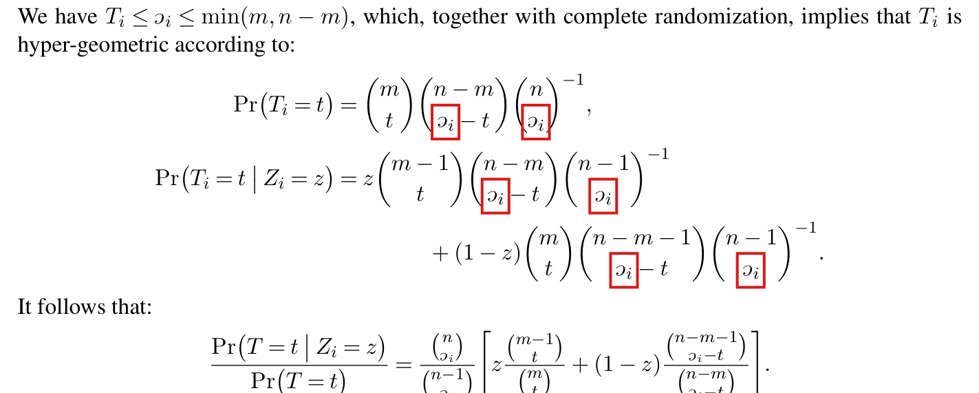
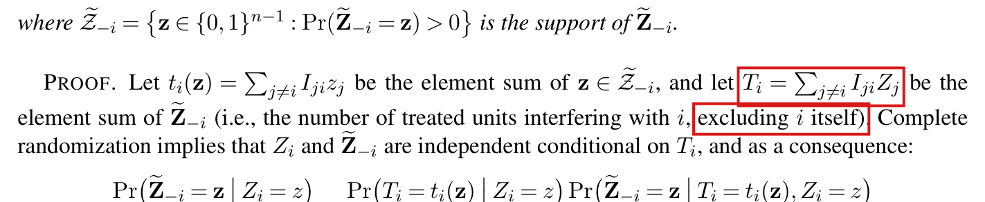
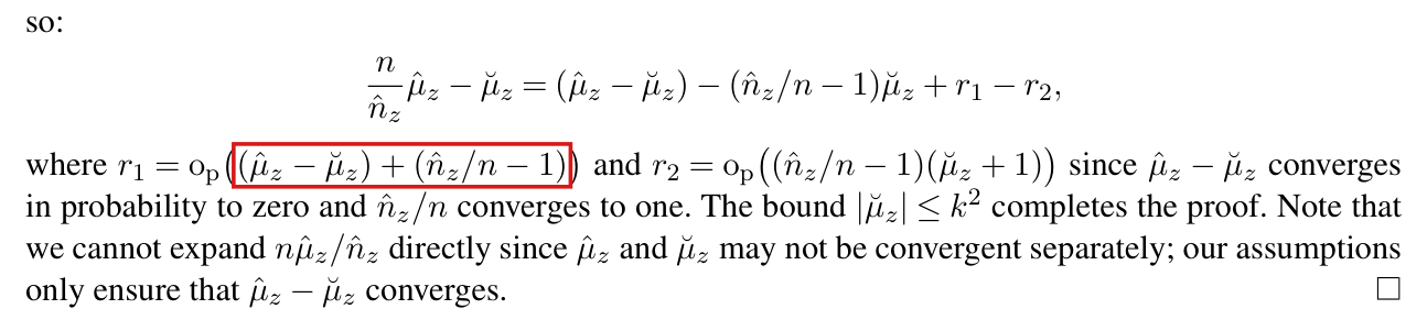
In the proof of Lemma A12, the variable TiT_i is hypergeometric with cˇi−1\check c_i-1 draws, not cˇi\check c_i, because the count cˇi\check c_i of Definition A3 includes unit ii and TiT_i does not; the inequality stated in the lemma holds unchanged.

Supplement A, proof of Lemma A12, p. 10 (PDF p. 10 of Supplement A), displays after “hyper-geometric according to:” and the ratio identities that follow; Definition A3 and the definition of TiT_i, p. 9

See also under Formal statements (Lean): P009-T17, P009-T18

As printed

Supplement A prints the count of Definition A3 as a reflected letter cc with subscript ii. It is written cˇi\check c_i here.

Definition A3, p. 9: “Let cˇi=∑j=1nIji\check c_i=\sum_{j=1}^n I_{ji} be the number of units interfering with unit ii.”

Proof of Lemma A12, p. 9: “let Ti=∑j≠iIjiZjT_i=\sum_{j\ne i}I_{ji}Z_j be the element sum of Z~−i\widetilde{\mathbf{Z}}_{-i} (i.e., the number of treated units interfering with ii, excluding ii itself).”

Proof of Lemma A12, p. 10: “We have Ti≤cˇi≤min⁡(m,n−m)T_i\le\check c_i\le\min(m,n-m), which, together with complete randomization, implies that TiT_i is hyper-geometric according to:

Pr⁡(Ti=t)=(mt)(n−mcˇi−t)(ncˇi)−1,\Pr\bigl(T_i=t\bigr)=\binom{m}{t}\binom{n-m}{\colorbox{#ffe58a}{$\displaystyle \check c_i$}-t}\binom{n}{\colorbox{#ffe58a}{$\displaystyle \check c_i$}}^{-1},
Pr⁡(Ti=t∣Zi=z)=z(m−1t)(n−mcˇi−t)(n−1cˇi)−1+(1−z)(mt)(n−m−1cˇi−t)(n−1cˇi)−1.”\begin{aligned} \Pr\bigl(T_i=t\mid Z_i=z\bigr)={}&z\binom{m-1}{t}\binom{n-m}{\colorbox{#ffe58a}{$\displaystyle \check c_i$}-t}\binom{n-1}{\colorbox{#ffe58a}{$\displaystyle \check c_i$}}^{-1}\\ &+(1-z)\binom{m}{t}\binom{n-m-1}{\colorbox{#ffe58a}{$\displaystyle \check c_i$}-t}\binom{n-1}{\colorbox{#ffe58a}{$\displaystyle \check c_i$}}^{-1}.\text{''} \end{aligned}

The ratio identities that follow end with

Pr⁡(Ti=t∣Zi=z)Pr⁡(Ti=t)−1=cˇiPr⁡(Zi=z)(n−cˇi)[Pr⁡(Zi=z)−ztcˇi−(1−z)cˇi−tcˇi],\frac{\Pr\bigl(T_i=t\mid Z_i=z\bigr)}{\Pr\bigl(T_i=t\bigr)}-1=\frac{\colorbox{#ffe58a}{$\displaystyle \check c_i$}}{\Pr(Z_i=z)(n-\colorbox{#ffe58a}{$\displaystyle \check c_i$})}\biggl[\Pr(Z_i=z)-z\frac{t}{\colorbox{#ffe58a}{$\displaystyle \check c_i$}}-(1-z)\frac{\colorbox{#ffe58a}{$\displaystyle \check c_i$}-t}{\colorbox{#ffe58a}{$\displaystyle \check c_i$}}\biggr],

and the proof concludes: “The expression within brackets is strictly between −1-1 and 11, so it follows:

∣Pr⁡(T=t∣Zi=z)Pr⁡(T=t)−1∣≤cˇiPr⁡(Zi=z)(n−cˇi)≤cˇiPr⁡(Zi=z)min⁡(m,n−m),”\biggl|\frac{\Pr\bigl(T=t\mid Z_i=z\bigr)}{\Pr\bigl(T=t\bigr)}-1\biggr|\le\frac{\check c_i}{\Pr(Z_i=z)(n-\check c_i)}\le\frac{\check c_i}{\Pr(Z_i=z)\min(m,n-m)},\text{''}
The problem

Definition A3 counts every unit that interferes with unit ii, and by the convention Iii=1I_{ii}=1 of the article (p. 680), unit ii is one of them. The variable TiT_i counts the treated units among the others, and there are cˇi−1\check c_i-1 of those. Under complete randomization, TiT_i is the number of treated units in a fixed set of cˇi−1\check c_i-1 units. Both printed laws, and the ratio identities derived from them, use one draw too many.

The error is confined to the proof. Using the correct number of draws in the same steps, I obtain a bound that is no larger than the one stated in Lemma A12. The lemma holds as stated.

Evidence an exact counterexample

The evidence is an exact counterexample to the printed laws and a derivation of the corrected ones. Let n=4n=4 and m=2m=2, and let the potential outcomes be y1(z)=z1+z2y_1(\mathbf{z})=z_1+z_2 and yj(z)=zjy_j(\mathbf{z})=z_j for j=2,3,4j=2,3,4. Then I11=I21=1I_{11}=I_{21}=1, cˇ1=2=min⁡(m,n−m)\check c_1=2=\min(m,n-m) and T1=Z2T_1=Z_2. Enumerating the six assignments, I find the laws in the following table.

Laws of T1T_1 in the example with n=4n=4, m=2m=2 and cˇ1=2\check c_1=2: enumeration of the six assignments, and the printed formulas.
ttPr⁡(T1=t)\Pr(T_1=t)printedPr⁡(T1=t∣Z1=1)\Pr(T_1=t\mid Z_1=1)printedPr⁡(T1=t∣Z1=0)\Pr(T_1=t\mid Z_1=0)printed
001/21/21/61/62/32/31/31/31/31/300
111/21/22/32/31/31/32/32/32/32/32/32/3
22001/61/60000001/31/3

For the corrected laws, let S={j≠i:Iji=1}S=\{j\ne i:I_{ji}=1\} and ri=∣S∣=cˇi−1r_i=|S|=\check c_i-1, so that Ti=∑j∈SZjT_i=\sum_{j\in S}Z_j. By the premise cˇi≤min⁡(m,n−m)\check c_i\le\min(m,n-m) of the lemma, I have ri<min⁡(m,n−m)r_i<\min(m,n-m). Counting the assignments with tt treated units in SS, I find

Pr⁡(Ti=t)=(rit)(n−rim−t)(nm)−1=(mt)(n−mri−t)(nri)−1.\Pr(T_i=t)=\binom{r_i}{t}\binom{n-r_i}{m-t}\binom{n}{m}^{-1}=\binom{m}{t}\binom{n-m}{r_i-t}\binom{n}{r_i}^{-1}.

Conditional on Zi=zZ_i=z, the other n−1n-1 units are completely randomized with m−zm-z treated units, and i∉Si\notin S. The same count with n−1n-1 and m−zm-z in place of nn and mm gives

Pr⁡(Ti=t∣Zi=z)=(m−zt)(n−1−m+zri−t)(n−1ri)−1.\Pr(T_i=t\mid Z_i=z)=\binom{m-z}{t}\binom{n-1-m+z}{r_i-t}\binom{n-1}{r_i}^{-1}.

These are the printed laws with rir_i in place of cˇi\check c_i. If ri=0r_i=0, then Ti=0T_i=0 and the ratio of the two probabilities is one. Suppose ri>0r_i>0, and let pz=Pr⁡(Zi=z)={zm+(1−z)(n−m)}/np_z=\Pr(Z_i=z)=\{zm+(1-z)(n-m)\}/n and uz=zt+(1−z)(ri−t)u_z=zt+(1-z)(r_i-t). Cancelling factorials as in the printed proof, I obtain

Pr⁡(Ti=t∣Zi=z)Pr⁡(Ti=t)−1=nn−ri[rin−ztm−(1−z)ri−tn−m]=ripz(n−ri)[pz−uzri].\frac{\Pr(T_i=t\mid Z_i=z)}{\Pr(T_i=t)}-1=\frac{n}{n-r_i}\biggl[\frac{r_i}{n}-z\frac{t}{m}-(1-z)\frac{r_i-t}{n-m}\biggr]=\frac{r_i}{p_z(n-r_i)}\biggl[p_z-\frac{u_z}{r_i}\biggr].

Since 0≤uz≤ri0\le u_z\le r_i and 0<pz<10<p_z<1, the last bracket lies strictly between −1-1 and 11. The inequality ri≤cˇir_i\le\check c_i implies that ri/(n−ri)≤cˇi/(n−cˇi)r_i/(n-r_i)\le\check c_i/(n-\check c_i), and n−cˇi≥max⁡(m,n−m)≥min⁡(m,n−m)n-\check c_i\ge\max(m,n-m)\ge\min(m,n-m). Combining these inequalities, I obtain the chain of inequalities in the corrected passage below. Note that the reduction from the vector Z~−i\widetilde{\mathbf{Z}}_{-i} to its sum TiT_i at the start of the printed proof is correct, since each pattern on SS with tt treated units has the same probability with and without the conditioning on ZiZ_i.

A check in rational arithmetic agrees with the derivation: the corrected laws match an enumeration of the assignments for every admissible (n,m,cˇi)(n,m,\check c_i) such that 2≤n≤102\le n\le10, and the chain of inequalities holds in all 61,60061{,}600 cases (n,m,cˇi,z,t)(n,m,\check c_i,z,t) such that 2≤n≤402\le n\le40. On that grid the left side is at most 19/4219/42 of the bound stated in the lemma.

What survives

Lemma A12 holds as stated, with the same assumptions and constant. Lemma A14, which applies the inequality of Lemma A12 on p. 14 of Supplement A, Proposition 3, the part of Corollary 1 on complete randomization, and the reference to Lemma A12 in Remark 1 on p. 688 use only that inequality and need no change. Only the two probability laws and the ratio identities inside the proof are corrected.

Corrected

Let ri=cˇi−1\colorbox{#ffe58a}{$r_i=\check c_i-1$} be the number of units other than ii that interfere with unit ii. The probability ratios below are for integers 0≤t≤ri0\le t\le r_i, the support of TiT_i. Since Ti≤ri<min⁡(m,n−m)T_i\le r_i<\min(m,n-m), complete randomization implies that TiT_i is hypergeometric according to:

Pr⁡(Ti=t)=(mt)(n−mri−t)(nri)−1,\Pr\bigl(T_i=t\bigr)=\binom{m}{t}\binom{n-m}{\colorbox{#ffe58a}{$\displaystyle r_i$}-t}\binom{n}{\colorbox{#ffe58a}{$\displaystyle r_i$}}^{-1},
Pr⁡(Ti=t∣Zi=z)=z(m−1t)(n−mri−t)(n−1ri)−1+(1−z)(mt)(n−m−1ri−t)(n−1ri)−1.\begin{aligned} \Pr\bigl(T_i=t\mid Z_i=z\bigr)={}&z\binom{m-1}{t}\binom{n-m}{\colorbox{#ffe58a}{$\displaystyle r_i$}-t}\binom{n-1}{\colorbox{#ffe58a}{$\displaystyle r_i$}}^{-1}\\ &+(1-z)\binom{m}{t}\binom{n-m-1}{\colorbox{#ffe58a}{$\displaystyle r_i$}-t}\binom{n-1}{\colorbox{#ffe58a}{$\displaystyle r_i$}}^{-1}. \end{aligned}

If ri=0r_i=0, then Ti=0T_i=0 and the ratio of the two probabilities is one. If ri>0r_i>0, the identities of the printed proof hold with rir_i in place of cˇi\check c_i and end with

Pr⁡(Ti=t∣Zi=z)Pr⁡(Ti=t)−1=riPr⁡(Zi=z)(n−ri)[Pr⁡(Zi=z)−ztri−(1−z)ri−tri].\frac{\Pr\bigl(T_i=t\mid Z_i=z\bigr)}{\Pr\bigl(T_i=t\bigr)}-1=\frac{\colorbox{#ffe58a}{$\displaystyle r_i$}}{\Pr(Z_i=z)(n-\colorbox{#ffe58a}{$\displaystyle r_i$})}\biggl[\Pr(Z_i=z)-z\frac{t}{\colorbox{#ffe58a}{$\displaystyle r_i$}}-(1-z)\frac{\colorbox{#ffe58a}{$\displaystyle r_i$}-t}{\colorbox{#ffe58a}{$\displaystyle r_i$}}\biggr].

The expression within brackets is strictly between −1-1 and 11, so in both cases

∣Pr⁡(Ti=t∣Zi=z)Pr⁡(Ti=t)−1∣≤riPr⁡(Zi=z)(n−ri)≤cˇiPr⁡(Zi=z)(n−cˇi)≤cˇiPr⁡(Zi=z)min⁡(m,n−m),\begin{aligned} \biggl|\frac{\Pr\bigl(T_i=t\mid Z_i=z\bigr)}{\Pr\bigl(T_i=t\bigr)}-1\biggr|&\le\frac{\colorbox{#ffe58a}{$\displaystyle r_i$}}{\Pr(Z_i=z)(n-\colorbox{#ffe58a}{$\displaystyle r_i$})}\\ &\le\frac{\check c_i}{\Pr(Z_i=z)(n-\check c_i)}\le\frac{\check c_i}{\Pr(Z_i=z)\min(m,n-m)}, \end{aligned}

where ri≤cˇi≤min⁡(m,n−m)≤max⁡(m,n−m)r_i\le\check c_i\le\min(m,n-m)\le\max(m,n-m) gives the last two inequalities. Definition A3 and the statement of Lemma A12 are unchanged.

Crop of the sentence 'We have T i at most reflected-c i at most min of m and n minus m, which, together with complete randomization, implies that T i is hyper-geometric according to' and the two displayed probability laws. Six red boxes mark the reflected letter c with subscript i in the lower entries of the binomial coefficients: two in the law of T i and four in the law of T i given Z i equals z.
Supplement A, proof of Lemma A12, p. 10. The six marked symbols are the numbers of draws in the two hypergeometric laws; each is the count cˇi\check c_i of Definition A3.
Crop of Definition A3. A red box marks the formula 'reflected-c i equals the sum over j from 1 to n of I j i', which is followed by the words 'be the number of units interfering with unit i'.
Supplement A, Definition A3, p. 9. The marked sum runs over all jj from 1 to nn, so it counts unit ii.
Crop of the first three lines of the proof of Lemma A12. Red boxes mark the formula 'T i equals the sum over j not equal to i of I j i Z j' and the words 'excluding i itself'.
Supplement A, start of the proof of Lemma A12, p. 9. The marked definition of TiT_i sums over j≠ij\ne i, and the marked words say that unit ii is excluded.

In the proof of Lemma A7 the first relation is printed as an equality and should be an inequality, since eije_{ij} is an indicator and the sum can exceed one.

Supplement A, proof of Lemma A7, foot of p. 5, first relation

See also under Formal statements (Lean): P009-T19, P009-T20, P009-T44

As printed

“Definition 7 gives eij=∑ℓ=1n(1−dij)IℓiIρ(ℓ)j≤∑ℓ=1nIℓiIρ(ℓ)je_{ij}\colorbox{#ffe58a}{$=$}\sum_{\ell=1}^n(1-d_{ij})I_{\ell i}I_{\rho(\ell)j}\le\sum_{\ell=1}^nI_{\ell i}I_{\rho(\ell)j}.”

The problem

Definition 7 (p. 685) sets eij=1e_{ij}=1 if (1−dij)IℓiIρ(ℓ)j=1(1-d_{ij})I_{\ell i}I_{\rho(\ell)j}=1 for some unit ℓ\ell, and eij=0e_{ij}=0 otherwise. The sum on the right counts the units ℓ\ell with this property, and several units can have it. The indicator is at most the sum and is not equal to it in general.

Evidence an exact counterexample

The evidence is an exact counterexample and a derivation. Let six units be paired as (1,2)(1,2), (3,4)(3,4), (5,6)(5,6), let every unit interfere with itself, and let I31=I51=I42=I62=1I_{31}=I_{51}=I_{42}=I_{62}=1 be the only other interference. The treatments that affect unit 11 are those of units 1,3,51,3,5, and the treatments that affect unit 22 are those of units 2,4,62,4,6. Since no treatment affects both units, I have d12=0d_{12}=0. By Definition 7, e12=1e_{12}=1, while the printed sum equals 33, with terms from ℓ=1,3,5\ell=1,3,5. With ≤\le in place of == the chain is valid for every interference structure and every pairing: an indicator that some term of a sum of zeros and ones equals one is at most the sum.

What survives

Lemma A7 and the results for the paired design that use it are unchanged. The proof uses only the upper bound eij≤∑ℓIℓiIρ(ℓ)je_{ij}\le\sum_{\ell}I_{\ell i}I_{\rho(\ell)j}, and the display on p. 6 is correct as printed.

Corrected

“Definition 7 gives eij≤∑ℓ=1n(1−dij)IℓiIρ(ℓ)j≤∑ℓ=1nIℓiIρ(ℓ)je_{ij}\colorbox{#ffe58a}{$\le$}\sum_{\ell=1}^n(1-d_{ij})I_{\ell i}I_{\rho(\ell)j}\le\sum_{\ell=1}^nI_{\ell i}I_{\rho(\ell)j}.”

The rest of the proof is as printed. With cℓ=∑i=1nIℓic_\ell=\sum_{i=1}^nI_{\ell i}, it gives, for every interference structure and every pairing ρ\rho,

eAVG≤1n∑i=1n∑j=1n∑ℓ=1nIℓiIρ(ℓ)j=1n∑ℓ=1ncℓcρ(ℓ)≤12n∑ℓ=1n(cℓ2+cρ(ℓ)2)=1n∑ℓ=1ncℓ2=C22.e_{\mathrm{AVG}}\le\frac1n\sum_{i=1}^n\sum_{j=1}^n\sum_{\ell=1}^nI_{\ell i}I_{\rho(\ell)j}=\frac1n\sum_{\ell=1}^nc_\ell c_{\rho(\ell)}\le\frac1{2n}\sum_{\ell=1}^n\big(c_\ell^2+c_{\rho(\ell)}^2\big)=\frac1n\sum_{\ell=1}^nc_\ell^2=C_2^2.
Crop showing Lemma A7, e_AVG is at most C_2 squared, and the first two lines of its proof. A red box marks the equality sign at the end of the first line, in 'Definition 7 gives e_ij ='. The next line continues with the sum over l of (1 - d_ij) I_li I_rho(l)j, followed by 'is at most' and the sum over l of I_li I_rho(l)j.
Supplement A, foot of p. 5: Lemma A7 and the first sentence of its proof. The marked sign should be ≤\le.

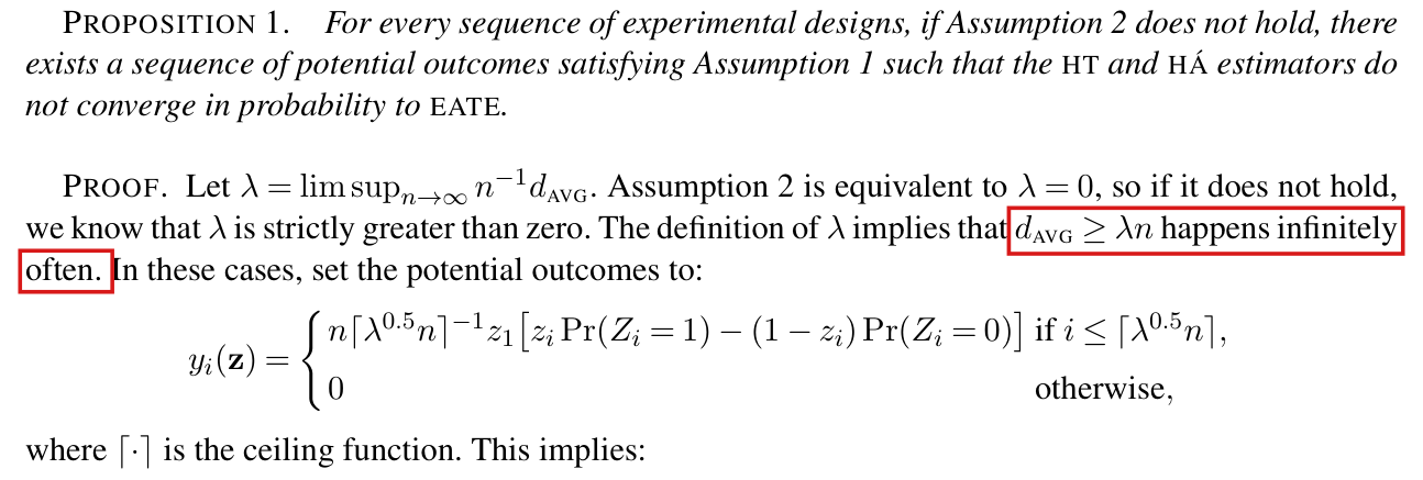
The proof of Proposition 1 asserts that dAVG≥λnd_{\mathrm{AVG}}\ge\lambda n infinitely often when λ\lambda is the limit superior of n−1dAVGn^{-1}d_{\mathrm{AVG}}, which can fail; the subsequence should be selected with a constant cc such that 0<c<λ0<c<\lambda.

Supplement A, Section 4, proof of Proposition 1, p. 6, first paragraph; the step is cited again in the last paragraph of the proof, p. 7

See also under Formal statements (Lean): P009-T5, P009-T6

As printed

“Proof. Let λ=lim sup⁡n→∞n−1dAVG\lambda=\limsup_{n\to\infty}n^{-1}d_{\mathrm{AVG}}. Assumption 2 is equivalent to λ=0\lambda=0, so if it does not hold, we know that λ\lambda is strictly greater than zero. The definition of λ\lambda implies that dAVG≥λnd_{\mathrm{AVG}}\ge\colorbox{#ffe58a}{$\lambda$}n happens infinitely often. In these cases, set the potential outcomes to: …”

Last paragraph of the proof, p. 7: “… with probability one whenever dAVG≥λnd_{\mathrm{AVG}}\ge\colorbox{#ffe58a}{$\lambda$}n, which, as we already noted, happens infinitely often.”

The problem

A sequence can stay strictly below its limit superior from some index on, and it then reaches or exceeds the limit superior only finitely often. The sample sizes with dAVG≥λnd_{\mathrm{AVG}}\ge\lambda n are those for which the proof constructs the potential outcomes and shows that ∣τ^HT−τEATE∣≥k−1|\hat\tau_{\mathrm{HT}}-\tau_{\mathrm{EATE}}|\ge k^{-1}. If there are finitely many of them, the argument as printed says nothing about convergence.

Evidence an exact counterexample

The evidence is an exact counterexample to the step. For each nn, let hn=max⁡{1,⌊n/2⌋−1}h_n=\max\{1,\lfloor n/2\rfloor-1\}, and let yi(z)=z1y_i(\mathbf{z})=z_1 for i≤hni\le h_n and yi(z)=0y_i(\mathbf{z})=0 otherwise. These potential outcomes lie in [0,1][0,1], and Assumption 1 holds with k=3k=3, for instance under complete randomization with ⌊n/2⌋\lfloor n/2\rfloor treated units when n≥2n\ge2. The treatment of unit 11 affects units 1,…,hn1,\dots,h_n, and every unit interferes with itself, so dij=1d_{ij}=1 if and only if i=ji=j or i,j≤hni,j\le h_n. I obtain

n−1dAVG=hn2+n−hnn2.n^{-1}d_{\mathrm{AVG}}=\frac{h_n^2+n-h_n}{n^2}.

For n=2mn=2m with m≥3m\ge3 this equals 1/4−(m−2)/(4m2)1/4-(m-2)/(4m^2), and for n=2m+1n=2m+1 with m≥2m\ge2 it equals 1/4−(8m−11)/(4(2m+1)2)1/4-(8m-11)/(4(2m+1)^2). These two expressions imply that λ=1/4\lambda=1/4 and n−1dAVG<λn^{-1}d_{\mathrm{AVG}}<\lambda for every n≥5n\ge5. The event dAVG≥λnd_{\mathrm{AVG}}\ge\lambda n occurs only for n≤4n\le4.

The repair is valid for the following reason. If 0<c<λ0<c<\lambda and n−1dAVG≥cn^{-1}d_{\mathrm{AVG}}\ge c held for finitely many nn only, then the limit superior would be at most cc, which is less than λ\lambda.

What survives

Proposition 1 and its use on p. 683 are unchanged, and the repair adds no assumption. The construction is kept with λ\lambda as printed: the constructed outcomes satisfy dAVG≥λnd_{\mathrm{AVG}}\ge\lambda n, are bounded by λ−0.5\lambda^{-0.5}, and give τEATE=Pr⁡(Z1=1)\tau_{\mathrm{EATE}}=\Pr(Z_1=1) and τ^HT=Z1\hat\tau_{\mathrm{HT}}=Z_1. The proof of Proposition 11 cites only the count of dAVGd_{\mathrm{AVG}} from this proof and is not affected. I did not assess the remark in the proof that the construction can be modified to replicate a specified sequence of dAVGd_{\mathrm{AVG}} exactly.

Corrected

“Proof. Let λ=lim sup⁡n→∞n−1dAVG\lambda=\limsup_{n\to\infty}n^{-1}d_{\mathrm{AVG}}. Assumption 2 is equivalent to λ=0\lambda=0, so if it does not hold, we know that λ\lambda is strictly greater than zero. Fix a constant c such that 0<c<λ.\colorbox{#ffe58a}{$\text{Fix a constant }c\text{ such that }0<c<\lambda.$} The definition of λ\lambda implies that dAVG≥cnd_{\mathrm{AVG}}\ge\colorbox{#ffe58a}{$c$}n happens infinitely often. In these cases, set the potential outcomes to:

yi(z)={n⌈λ0.5n⌉−1z1[ziPr⁡(Zi=1)−(1−zi)Pr⁡(Zi=0)]if i≤⌈λ0.5n⌉,0otherwise,y_i(\mathbf{z})=\begin{cases}n\lceil\lambda^{0.5}n\rceil^{-1}z_1\big[z_i\Pr(Z_i=1)-(1-z_i)\Pr(Z_i=0)\big]&\text{if }i\le\lceil\lambda^{0.5}n\rceil,\\0&\text{otherwise,}\end{cases}

where ⌈⋅⌉\lceil\cdot\rceil is the ceiling function.”

In the last paragraph of the proof, p. 7: “… with probability one whenever dAVG≥cnd_{\mathrm{AVG}}\ge\colorbox{#ffe58a}{$c$}n, which, as we already noted, happens infinitely often.”

The constant λ\lambda stays in the construction, so that the limit superior of n−1dAVGn^{-1}d_{\mathrm{AVG}} for the constructed outcomes is still λ\lambda. For the sample sizes with dAVG<cnd_{\mathrm{AVG}}<cn, all potential outcomes may be set to zero.

Crop showing Proposition 1 and the start of its proof, which defines lambda as the limit superior of d_AVG over n. A red box marks the words 'd_AVG is at least lambda n happens infinitely often', which run over two lines. Below, the display defines the potential outcomes y_i(z) for i up to the ceiling of lambda to the power 0.5 times n.
Supplement A, p. 6: Proposition 1 and the first paragraph of its proof. The marked clause does not follow from the definition of the limit superior.

The two limits follow from an upper bound, (1−1/k)bn→0(1 - 1/k)^{b_n} \to 0, on the probability of each support point of zSUB,n\mathbf{z}_{\mathrm{SUB},n} and not from the lower bound k−bnk^{-b_n}, and z′\mathbf{z}' should read zSUB,n\mathbf{z}_{\mathrm{SUB},n}.

Supplement A, p. 37, proof of Proposition 11, first paragraph of the page

See also under Formal statements (Lean): P009-T27

As printed

The Bernoulli design and Assumption 1 imply that the support of z′\colorbox{#ffe58a}{$\mathbf{z}'$} consists of 2bn2^{b_n} points each with a probability of at least k−bn\colorbox{#ffe58a}{$k^{-b_n}$}. It follows that:

lim⁡n→∞Pr⁡(fn∗(zSUB,n)=1)=α/2andlim⁡n→∞Pr⁡(fn∗(zSUB,n)=−1)=α/2.\lim_{n \to \infty}\Pr\bigl(f_n^*(\mathbf{z}_{\mathrm{SUB},n}) = 1\bigr) = \alpha/2 \qquad \text{and} \qquad \lim_{n \to \infty}\Pr\bigl(f_n^*(\mathbf{z}_{\mathrm{SUB},n}) = -1\bigr) = \alpha/2.
The problem

The function fn∗f_n^* is chosen on p. 36 to bring Pr⁡(f(zSUB,n)=1)\Pr(f(\mathbf{z}_{\mathrm{SUB},n}) = 1) and Pr⁡(f(zSUB,n)=−1)\Pr(f(\mathbf{z}_{\mathrm{SUB},n}) = -1) as close to α/2\alpha/2 as possible. To ensure that sets of support points can approach these two masses, it is enough that the largest point probability tends to zero. The printed lower bound on the probability of each point does not ensure that: a distribution on 2b2^{b} points can satisfy such a lower bound while one point carries almost all of the mass. The bound that is needed is the upper bound (1−1/k)bn(1 - 1/k)^{b_n}, which follows from the same assumptions. The symbol z′\mathbf{z}' is also not defined, and the vector zSUB,n\mathbf{z}_{\mathrm{SUB},n} introduced on p. 36 is meant.

Evidence a derivation

The evidence is a derivation. By Assumption 1A, I have k−1≤Pr⁡(Zi=1)≤1−k−1k^{-1} \leq \Pr(Z_i = 1) \leq 1 - k^{-1} for every unit. Since the assignments are independent under a Bernoulli design, every support point a\mathbf{a} of zSUB,n\mathbf{z}_{\mathrm{SUB},n} satisfies

k−bn≤Pr⁡(zSUB,n=a)≤δn,δn=(1−1/k)bn,k^{-b_n} \leq \Pr(\mathbf{z}_{\mathrm{SUB},n} = \mathbf{a}) \leq \delta_n, \qquad \delta_n = (1 - 1/k)^{b_n},

and δn→0\delta_n \to 0 because bn→∞b_n \to \infty. The lower bound alone is not enough. Suppose that a distribution on 2b2^b points assigns one point the probability 1−(2b−1)4−b1 - (2^b - 1)4^{-b} and every other point the probability 4−b4^{-b}. Then every point has probability at least 4−b4^{-b}, which is the printed lower bound with k=4k = 4. The largest probability tends to one, and no set of points has probability near α/2\alpha/2 for α∈(0,1)\alpha \in (0, 1). This distribution is not a Bernoulli design, and it serves only to test the implication. With the upper bound, I order the support points and take the longest initial segments whose total probabilities are at most α/2\alpha/2 and at most α\alpha. Each total falls short of its target by less than δn\delta_n. Let ff equal 11 on the first segment, −1-1 on the rest of the second, and 00 elsewhere. With this choice, Pr⁡(f=1)\Pr(f = 1) and Pr⁡(f=−1)\Pr(f = -1) are each within δn\delta_n of α/2\alpha/2. The total error of the minimizer fn∗f_n^* is no larger than the total error of this function, which is at most 2δn2\delta_n, and this implies both limits.

What survives

Both limits hold, and with them the convergence in distribution on which Proposition 11 rests. No assumption is added. The comparison that uses these limits later in the proof is corrected in P009-E017.

Corrected

The Bernoulli design and Assumption 1 imply that the support of zSUB,n\colorbox{#ffe58a}{$\mathbf{z}_{\mathrm{SUB},n}$} consists of 2bn2^{b_n} points, each with a probability of at most (1−1/k)bn\colorbox{#ffe58a}{$(1 - 1/k)^{b_n}$}, which tends to zero. Disjoint sets of support points can then approximate the two target masses α/2\alpha/2, and the minimizing fn∗f_n^* satisfies

lim⁡n→∞Pr⁡(fn∗(zSUB,n)=1)=α/2andlim⁡n→∞Pr⁡(fn∗(zSUB,n)=−1)=α/2.\lim_{n \to \infty}\Pr\bigl(f_n^*(\mathbf{z}_{\mathrm{SUB},n}) = 1\bigr) = \alpha/2 \qquad \text{and} \qquad \lim_{n \to \infty}\Pr\bigl(f_n^*(\mathbf{z}_{\mathrm{SUB},n}) = -1\bigr) = \alpha/2.
Crop of the top of p. 37, with the running head Supplement A: Proofs and the page number 37. The text reads: The Bernoulli design and Assumption 1 imply that the support of z prime consists of 2 to the b n points each with a probability of at least k to the minus b n. It follows that: the limit as n tends to infinity of Pr(f star n of z SUB,n = 1) = alpha over 2, and the limit as n tends to infinity of Pr(f star n of z SUB,n = minus 1) = alpha over 2. Red outlines surround the symbol z prime in the first line and the words at least k to the minus b n in the second.
Supplement A, p. 37, top of the page, in the proof of Proposition 11. The outlines mark the undefined symbol z′\mathbf{z}' and the lower bound “at least k−bnk^{-b_n}”.

The comparison is reversed and lacks an absolute value: for all large nn the distance from ss to {−1,0,1}\{-1, 0, 1\} is greater than ∣Pr⁡(fn∗=1)−Pr⁡(fn∗=−1)∣|\Pr(f_n^* = 1) - \Pr(f_n^* = -1)|.

Supplement A, p. 38, proof of Proposition 11, sentence beginning “Hence, for any fixed ss”

See also under Formal statements (Lean): P009-T28

As printed

Hence, for any fixed s∈R∖{−1,0,1}s \in \mathbb{R} \setminus \{-1, 0, 1\}, there exists an n′n' such that the smallest distance from ss to any point in {−1,0,1}\{-1, 0, 1\} for all n≥n′n \geq n' is less than:

Pr⁡(fn∗(zSUB,n)=1)−Pr⁡(fn∗(zSUB,n)=−1).\Pr\bigl(f_n^*(\mathbf{z}_{\mathrm{SUB},n}) = 1\bigr) - \Pr\bigl(f_n^*(\mathbf{z}_{\mathrm{SUB},n}) = -1\bigr).
The problem

For a fixed ss outside {−1,0,1}\{-1, 0, 1\} the distance δs\delta_s from ss to that set is positive and does not depend on nn. The displayed difference, μn\mu_n say, tends to zero by the display that precedes the sentence. A fixed positive number cannot be less than μn\mu_n for all large nn, and μn\mu_n may be negative. The next display of the proof needs the opposite comparison with an absolute value, ∣μn∣<δs|\mu_n| < \delta_s, which does hold for all large nn. A further misprint in the last display of the proof, xx for ss, is the subject of P009-E020.

Evidence a derivation

The evidence is a derivation. Let Fn=fn∗(zSUB,n)F_n = f_n^*(\mathbf{z}_{\mathrm{SUB},n}), which takes values in {−1,0,1}\{-1, 0, 1\}, and let μn=E[Fn]=Pr⁡(Fn=1)−Pr⁡(Fn=−1)\mu_n = \mathrm{E}[F_n] = \Pr(F_n = 1) - \Pr(F_n = -1). By the display headed “Taken together” on p. 38, the normalized estimator equals Fn−μnF_n - \mu_n. Suppose that ∣μn∣<δs|\mu_n| < \delta_s. Then no point of {−1,0,1}\{-1, 0, 1\} lies between ss and s+μns + \mu_n, so for each t∈{−1,0,1}t \in \{-1, 0, 1\} the inequalities t≤st \leq s and t≤s+μnt \leq s + \mu_n are equivalent, and I have

Pr⁡(Fn−μn≤s)=Pr⁡(Fn≤s+μn)=Pr⁡(Fn≤s),\Pr(F_n - \mu_n \leq s) = \Pr(F_n \leq s + \mu_n) = \Pr(F_n \leq s),

which is the next display of the proof. Since μn→0\mu_n \to 0, the condition ∣μn∣<δs|\mu_n| < \delta_s holds for all large nn. The limits of Pr⁡(Fn=1)\Pr(F_n = 1) and Pr⁡(Fn=−1)\Pr(F_n = -1) used here are those justified in P009-E016.

What survives

The equality of distribution functions in the next display holds for all large nn under the corrected condition, and the convergence in distribution claimed in the proof is preserved. Nothing else in the proof changes.

Corrected

Hence, for any fixed s∈R∖{−1,0,1}s \in \mathbb{R} \setminus \{-1, 0, 1\}, there exists an n′n' such that, for all n≥n′n \geq n', the smallest distance from ss to any point in {−1,0,1}\{-1, 0, 1\} is greater than:

∣Pr⁡(fn∗(zSUB,n)=1)−Pr⁡(fn∗(zSUB,n)=−1)∣.\colorbox{#ffe58a}{$\displaystyle \Bigl|$}\Pr\bigl(f_n^*(\mathbf{z}_{\mathrm{SUB},n}) = 1\bigr) - \Pr\bigl(f_n^*(\mathbf{z}_{\mathrm{SUB},n}) = -1\bigr)\colorbox{#ffe58a}{$\displaystyle \Bigr|$}.
Crop of part of a proof. A first display states that the limit as n tends to infinity of the bracket Pr(f star n of z SUB,n = 1) minus Pr(f star n of z SUB,n = minus 1) equals 0. The text reads: Hence, for any fixed s in the real numbers without minus 1, 0 and 1, there exists an n prime such that the smallest distance from s to any point in the set of minus 1, 0 and 1 for all n at least n prime is less than: followed by the displayed difference Pr(f star n of z SUB,n = 1) minus Pr(f star n of z SUB,n = minus 1). Red outlines surround the words is less than and the displayed difference. The text continues: For the s under consideration and all such n at least n prime, and a last display states that Pr(n to the 0.5 d AVG to the minus 0.5 times (tau-hat HT minus E of tau-hat HT) is at most s) = Pr(f star n of z SUB,n is at most s).
Supplement A, p. 38, proof of Proposition 11. The outlines mark the words “is less than” and the difference of probabilities, printed without an absolute value, to which the distance is compared.

In the first line of the proof of Lemma A3 the outcome of unit jj is printed twice as YiaY_i^a; both should read YjaY_j^a.

Supplement A, proof of Lemma A3, p. 3 (PDF p. 3 of the supplement), first line of the display

See also under Formal statements (Lean): P009-T29

As printed

“Proof. The Cauchy–Schwarz inequality gives:”

Cov⁡(1[Zi=z]Yia,1[Zj=z]Yia)≤[Var⁡(1[Zi=z]Yia)Var⁡(1[Zj=z]Yia)]0.5\operatorname{Cov}\big(\mathbf{1}[Z_i=z]Y_i^a,\mathbf{1}[Z_j=z]\colorbox{#ffe58a}{$\displaystyle Y_i^a$}\big)\le\Big[\operatorname{Var}\big(\mathbf{1}[Z_i=z]Y_i^a\big)\operatorname{Var}\big(\mathbf{1}[Z_j=z]\colorbox{#ffe58a}{$\displaystyle Y_i^a$}\big)\Big]^{0.5}
The problem

Lemma A3 bounds the covariance of 1[Zi=z]Yia\mathbf{1}[Z_i=z]Y_i^a and 1[Zj=z]Yja\mathbf{1}[Z_j=z]Y_j^a, and the second line of its proof has E[∣Yj∣2a]\mathrm{E}[|Y_j|^{2a}]. The first line carries YiaY_i^a in the second argument of the covariance and in the second variance. As printed, the line is a valid Cauchy–Schwarz inequality, but for a covariance other than the one in the lemma, and the second line does not follow from it.

Evidence a check of the printed page

The evidence is a check of the page and a derivation. Let Xi=1[Zi=z]YiaX_i=\mathbf{1}[Z_i=z]Y_i^a and Xj=1[Zj=z]YjaX_j=\mathbf{1}[Z_j=z]Y_j^a. For r∈{i,j}r\in\{i,j\}, I have Var⁡(Xr)≤E[Xr2]≤E[∣Yr∣2a]\operatorname{Var}(X_r)\le\mathrm{E}[X_r^2]\le\mathrm{E}[|Y_r|^{2a}]. Using the Cauchy–Schwarz inequality, I obtain Cov⁡(Xi,Xj)≤[E[∣Yi∣2a] E[∣Yj∣2a]]0.5\operatorname{Cov}(X_i,X_j)\le[\mathrm{E}[|Y_i|^{2a}]\,\mathrm{E}[|Y_j|^{2a}]]^{0.5}, which is the second line of the proof. For q≥2aq\ge2a, Jensen’s inequality and Assumption 1B imply that E[∣Yr∣2a]≤E[∣Yr∣q]2a/q≤k2a\mathrm{E}[|Y_r|^{2a}]\le\mathrm{E}[|Y_r|^q]^{2a/q}\le k^{2a}, and the bound k2ak^{2a} of the lemma follows.

What survives

Lemma A3 holds as stated, and its proof is unchanged from the second line on.

Corrected

In the proof of Lemma A3 (Assumption 1B with q≥2aq\ge2a), for all i,j∈Ui,j\in\mathbf{U} and z∈{0,1}z\in\{0,1\}:

Cov⁡(1[Zi=z]Yia,1[Zj=z]Yja)≤[Var⁡(1[Zi=z]Yia)Var⁡(1[Zj=z]Yja)]0.5\operatorname{Cov}\big(\mathbf{1}[Z_i=z]Y_i^a,\mathbf{1}[Z_j=z]\colorbox{#ffe58a}{$\displaystyle Y_j^a$}\big)\le\Big[\operatorname{Var}\big(\mathbf{1}[Z_i=z]Y_i^a\big)\operatorname{Var}\big(\mathbf{1}[Z_j=z]\colorbox{#ffe58a}{$\displaystyle Y_j^a$}\big)\Big]^{0.5}

The remaining lines of the display are as printed.

Crop showing Lemma A3, whose statement bounds the covariance of 1[Z_i = z] Y_i^a and 1[Z_j = z] Y_j^a by k^(2a), and the first three lines of the proof. In the first line of the proof, red boxes mark the term Y_i^a in the second argument of the covariance and the term Y_i^a in the second variance. The second line has the expectations of |Y_i|^(2a) and |Y_j|^(2a).
Supplement A, p. 3: Lemma A3 and the first lines of its proof. The two marked terms carry the index ii where the statement of the lemma and the second line of the proof have jj.

The subscript AVG should read MAX in the proof of Proposition 9 and SR in the proof of Proposition 10.

Supplement A, p. 34, proof of Proposition 9, and p. 35, proof of Proposition 10: in each, the sentence that applies Corollary A4

See also under Formal statements (Lean): P009-T30, P009-T49, P009-T50

As printed

Page 34: The second premise is satisfied by Corollary A4 because Var⁡^AVG(τ^HT)=bnVar⁡^BER(τ^HT)\widehat{\operatorname{Var}}_{\colorbox{#ffe58a}{$\mathrm{AVG}$}}(\hat\tau_{\mathrm{HT}}) = b_n\widehat{\operatorname{Var}}_{\mathrm{BER}}(\hat\tau_{\mathrm{HT}}) and bn=dMAX=o(n0.5dAVG0.5)b_n = d_{\mathrm{MAX}} = o(n^{0.5}d_{\mathrm{AVG}}^{0.5}) by assumption.

Page 35: The second premise is satisfied by Corollary A4 because Var⁡^AVG(τ^HT)=bnVar⁡^BER(τ^HT)\widehat{\operatorname{Var}}_{\colorbox{#ffe58a}{$\mathrm{AVG}$}}(\hat\tau_{\mathrm{HT}}) = b_n\widehat{\operatorname{Var}}_{\mathrm{BER}}(\hat\tau_{\mathrm{HT}}) and bn=λmax⁡=o(n0.5dAVG0.5)b_n = \lambda_{\max} = o(n^{0.5}d_{\mathrm{AVG}}^{0.5}) by assumption.

The problem

The article defines Var⁡^AVG=dAVGVar⁡^BER\widehat{\operatorname{Var}}_{\mathrm{AVG}} = d_{\mathrm{AVG}}\widehat{\operatorname{Var}}_{\mathrm{BER}}, Var⁡^MAX=dMAXVar⁡^BER\widehat{\operatorname{Var}}_{\mathrm{MAX}} = d_{\mathrm{MAX}}\widehat{\operatorname{Var}}_{\mathrm{BER}} and Var⁡^SR=λmax⁡Var⁡^BER\widehat{\operatorname{Var}}_{\mathrm{SR}} = \lambda_{\max}\widehat{\operatorname{Var}}_{\mathrm{BER}} (pp. 691–693). The two proofs set bn=dMAXb_n = d_{\mathrm{MAX}} and bn=λmax⁡b_n = \lambda_{\max}, so the estimator that equals bnVar⁡^BERb_n\widehat{\operatorname{Var}}_{\mathrm{BER}} is Var⁡^MAX\widehat{\operatorname{Var}}_{\mathrm{MAX}} in the first and Var⁡^SR\widehat{\operatorname{Var}}_{\mathrm{SR}} in the second.

Evidence a check of the printed page

The evidence is a check of the two pages against the definitions on pp. 691–693 of the article and against the opening of each proof, where bnb_n is chosen.

What survives

Propositions 9 and 10 and their proofs are unaffected. The multiplier bnb_n and every bound are the intended ones, and only the label of the estimator changes.

Corrected

Page 34: The second premise is satisfied by Corollary A4 because Var⁡^MAX(τ^HT)=bnVar⁡^BER(τ^HT)\widehat{\operatorname{Var}}_{\colorbox{#ffe58a}{$\mathrm{MAX}$}}(\hat\tau_{\mathrm{HT}}) = b_n\widehat{\operatorname{Var}}_{\mathrm{BER}}(\hat\tau_{\mathrm{HT}}) and bn=dMAX=o(n0.5dAVG0.5)b_n = d_{\mathrm{MAX}} = o(n^{0.5}d_{\mathrm{AVG}}^{0.5}) by assumption.

Page 35: The second premise is satisfied by Corollary A4 because Var⁡^SR(τ^HT)=bnVar⁡^BER(τ^HT)\widehat{\operatorname{Var}}_{\colorbox{#ffe58a}{$\mathrm{SR}$}}(\hat\tau_{\mathrm{HT}}) = b_n\widehat{\operatorname{Var}}_{\mathrm{BER}}(\hat\tau_{\mathrm{HT}}) and bn=λmax⁡=o(n0.5dAVG0.5)b_n = \lambda_{\max} = o(n^{0.5}d_{\mathrm{AVG}}^{0.5}) by assumption.

Crop of part of a proof. The text reads: Consider the first case in the proposition using Lemma A27. By construction, tau MSQ is at least 0 and b n times d AVG to the minus 1 equals d AVG to the minus 1 times d MAX, which is at least 1, so: a displayed inequality states that the limit inferior of b n d AVG to the minus 1 times the bracket a n minus n b n to the minus 1 Var of tau-hat HT is at least the limit inferior of tau MSQ, which is at least 0. The text continues: and the first premise of the lemma is satisfied without invoking additional assumptions. The second premise is satisfied by Corollary A4 because Var-hat AVG of tau-hat HT = b n times Var-hat BER of tau-hat HT and b n = d MAX = o(n to the 0.5 times d AVG to the 0.5) by assumption. A red outline surrounds Var-hat AVG of tau-hat HT. The crop ends: Consider the second case in the proposition using Lemma A28. By assumption: the limit inferior of tau MSQ is at least c, which is greater than 0, so.
Supplement A, p. 34, proof of Proposition 9. The outline marks the estimator printed with the subscript AVG, in a sentence where bn=dMAXb_n = d_{\mathrm{MAX}}.
Crop of the last lines of p. 35. A displayed inequality states that the limit inferior of b n d AVG to the minus 1 times the bracket a n minus n b n to the minus 1 Var of tau-hat HT is at least the limit inferior of tau MSQ, which is at least 0. The text reads: and the first premise of the lemma is satisfied without invoking additional assumptions. The second premise is satisfied by Corollary A4 because Var-hat AVG of tau-hat HT = b n times Var-hat BER of tau-hat HT and b n = lambda max = o(n to the 0.5 times d AVG to the 0.5) by assumption. A red outline surrounds Var-hat AVG of tau-hat HT.
Supplement A, p. 35, proof of Proposition 10. The outline marks the same estimator, again with the subscript AVG, in a sentence where bn=λmax⁡b_n = \lambda_{\max}.

The article and Supplement A should read “to capture”, “social structure. Paired units”, “moderate interference”, “is governed”, “subtract” and “converges”, and the four cases of the last display in the proof of Proposition 11 should be written in ss, not xx.

Article, p. 686 (PDF p. 14) and p. 697 (PDF p. 25); Supplement A, pp. 4, 28, 29, 36 and 38 (the same PDF pages of Supplement A)

See also under Formal statements (Lean): P009-T31

As printed
  • Article, p. 686: “The purpose of Definition 8 is to captures how common interference is between paired units.”
  • Article, p. 686: “It is, for example, common that the pairs reflect some social structure Paired units may, for example, live in the same household.”
  • Article, p. 697: “experiments often are informative of EATE even in the presence of moderate inference with unknown form.”
  • Supplement A, Lemma A5, p. 4: “If the rate of convergence in the L2L_2-norm for a sequence of random variables is govern by a sequence (an)(a_n), then the rate of convergence in probability is govern by (an)(a_n).”
  • Supplement A, proof of Proposition 7, p. 28 (twice) and p. 29 (once): “Add and substract:”
  • Supplement A, proof of Proposition 11, p. 36: “the normalized sampling distribution of the HT estimator convergence in distribution to the random variable in Definition A4”
  • Supplement A, proof of Proposition 11, p. 38:
    lim⁡n→∞Pr⁡(fn∗(zSUB,n)≤s)=Pr⁡(X(α)≤s)={0if x<−1,α/2if x<0,1−α/2if x<1,1if x≥1.\lim_{n\to\infty}\Pr\bigl(f_n^*(\mathbf{z}_{\mathrm{SUB},n})\le s\bigr)=\Pr\bigl(X(\alpha)\le s\bigr)=\begin{cases}0&\text{if }\colorbox{#ffe58a}{$\displaystyle x$}<-1,\\ \alpha/2&\text{if }\colorbox{#ffe58a}{$\displaystyle x$}<0,\\ 1-\alpha/2&\text{if }\colorbox{#ffe58a}{$\displaystyle x$}<1,\\ 1&\text{if }\colorbox{#ffe58a}{$\displaystyle x$}\ge1.\end{cases}
The problem

These are misprints, and in each case the sentence shows the intended wording. In the display on p. 38 of Supplement A, the left side is a distribution function evaluated at ss, and the four cases are written in xx. The paragraph before the display restricts ss to R∖{−1,0,1}\mathbb{R}\setminus\{-1,0,1\}, and for those ss the four cases, read in order, are the distribution function of the random variable X(α)X(\alpha) of Definition A4.

Evidence a check of the printed page

I checked each listed misprint on the pages of the article and Supplement A.

What survives

No mathematical statement changes.

Corrected
  • Article, p. 686: “The purpose of Definition 8 is to capture how common interference is between paired units.”
  • Article, p. 686: “It is, for example, common that the pairs reflect some social structure. Paired units may, for example, live in the same household.”
  • Article, p. 697: “even in the presence of moderate interference with unknown form.”
  • Supplement A, Lemma A5: “is governed by a sequence (an)(a_n), then the rate of convergence in probability is governed by (an)(a_n).”
  • Supplement A, pp. 28 and 29: “Add and subtract:”
  • Supplement A, p. 36: “the HT estimator converges in distribution to the random variable in Definition A4”
  • Supplement A, p. 38:
    lim⁡n→∞Pr⁡(fn∗(zSUB,n)≤s)=Pr⁡(X(α)≤s)={0if s<−1,α/2if s<0,1−α/2if s<1,1if s≥1.\lim_{n\to\infty}\Pr\bigl(f_n^*(\mathbf{z}_{\mathrm{SUB},n})\le s\bigr)=\Pr\bigl(X(\alpha)\le s\bigr)=\begin{cases}0&\text{if }\colorbox{#ffe58a}{$\displaystyle s$}<-1,\\ \alpha/2&\text{if }\colorbox{#ffe58a}{$\displaystyle s$}<0,\\ 1-\alpha/2&\text{if }\colorbox{#ffe58a}{$\displaystyle s$}<1,\\ 1&\text{if }\colorbox{#ffe58a}{$\displaystyle s$}\ge1.\end{cases}
    For a display that is valid at every ss, the four ranges are s<−1s<-1, −1≤s<0-1\le s<0, 0≤s<10\le s<1 and s≥1s\ge1.
Crop of six lines of text. Red boxes mark the words 'is to' at the end of one line and 'captures' at the start of the next, in the sentence 'The purpose of Definition 8 is to captures how common interference is between paired units'.
Article, p. 686 (PDF p. 14). The marked words read “is to captures”.
Crop of four lines of text. A red box marks the words 'structure Paired' in 'the pairs reflect some social structure Paired units may, for example, live in the same household'.
Article, p. 686 (PDF p. 14). No full stop separates the marked words “structure” and “Paired”.
Crop of five lines of text from the concluding section. A red box marks the word 'inference' in 'even in the presence of moderate inference with unknown form'.
Article, p. 697 (PDF p. 25). The marked word is “inference”.
Crop of the statement of Lemma A5 and the first line of its proof. Red boxes mark the word 'govern' in 'is govern by a sequence a n' and in 'the rate of convergence in probability is govern by a n'.
Supplement A, Lemma A5, p. 4. The marked word “govern” appears twice.
Crop of several displayed equations with connecting text. Red boxes mark the word 'substract' in two sentences that read 'Add and substract'.
Supplement A, proof of Proposition 7, p. 28. The marked word “substract” appears twice.
Crop of two displayed equations with one line of text between them. A red box marks the word 'substract' in 'Add and substract'.
Supplement A, proof of Proposition 7, p. 29. The marked word is “substract”.
Crop of the first four lines of the proof of Proposition 11. A red box marks the word 'convergence' in 'the normalized sampling distribution of the HT estimator convergence in distribution to the random variable in Definition A4'.
Supplement A, proof of Proposition 11, p. 36. The marked word is “convergence”.
Crop of the last display of the proof of Proposition 11, which gives the limit of a probability evaluated at s as a function with four cases. Four red boxes mark the letter x in the conditions 'if x less than minus 1', 'if x less than 0', 'if x less than 1' and 'if x at least 1'.
Supplement A, end of the proof of Proposition 11, p. 38. The argument on the left of the display is ss; the four marked conditions are written in xx.

The explanation on p. 6 says that changing one unit’s assignment moves bal⁡(Gj)\operatorname{bal}(G_j) by one; it moves it by two.

Supplement B, Section 1.2, p. 6, paragraphs beginning “To understand this behavior” and “Now consider the same situation”

See also under Formal statements (Lean): P009-T32

As printed

“Of the units in Gi\mathcal{G}_i, some fraction will have bal⁡(Gj)=0\operatorname{bal}(G_j)=0. When we change ii's assignment, those units will change to bal⁡(Gj)=1\operatorname{bal}(G_j)=\colorbox{#ffe58a}{$1$}, and thus change the values of their outcomes. Similarly, some other fraction of Gi\mathcal{G}_i will have bal⁡(Gj)=−1\operatorname{bal}(G_j)=-1, and their values will change to bal⁡(Gj)=0\operatorname{bal}(G_j)=\colorbox{#ffe58a}{$0$}.”

Next paragraph: “… when we change ii's assignment from control to treatment and add one to bal⁡(Gj)\operatorname{bal}(G_j) for the units in Gi\mathcal{G}_i, a counteracting effect happens because we simultaneously change ℓ\ell's assignment from treatment to control and remove one from bal⁡(Gj)\operatorname{bal}(G_j) for units in Gℓ\mathcal{G}_\ell. The number of units that get one added to bal⁡(Gj)\operatorname{bal}(G_j) will, with high probability and relative to the sample size, be close to the number of units that get one removed …”

The problem

The balance is bal⁡(Gj)=∑l∈Gj(2Zl−1)\operatorname{bal}(G_j)=\sum_{l\in G_j}(2Z_l-1) (p. 2). When unit i∈Gji\in G_j moves from control to treatment, its term changes from −1-1 to +1+1, and the balance increases by two. The values after the change are 22 and 11, not 11 and 00, and the second paragraph should add and remove two.

Evidence a derivation

The evidence is a derivation from the definition of the balance. The coefficient of zjz_j in the outcome of unit jj is 00, 11 or 22 according as the balance is negative, zero or positive. An increase of two changes this coefficient exactly when the balance starts at −2-2, −1-1 or 00, and a decrease of two changes it exactly when the balance starts at 00, 11 or 22. The simulation code in Supplement C computes the balance from the terms 2Zl−12Z_l-1, and the simulations do not contain the slip.


What survives

The qualitative explanation is unchanged: the sign of the balance changes for some units, and moving a second unit in the opposite direction counteracts the first change. The set {0,1}\{0,1\} in the second paragraph can stay, since the sentence speaks of some fraction of the units; the starting values from which a decrease changes the outcome are 00, 11 and 22. I did not check any statement about the size of these fractions.
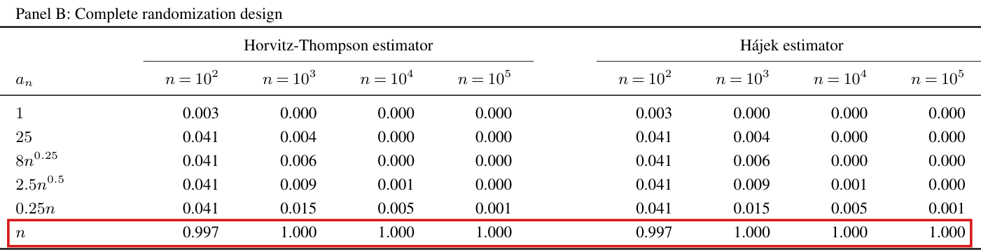
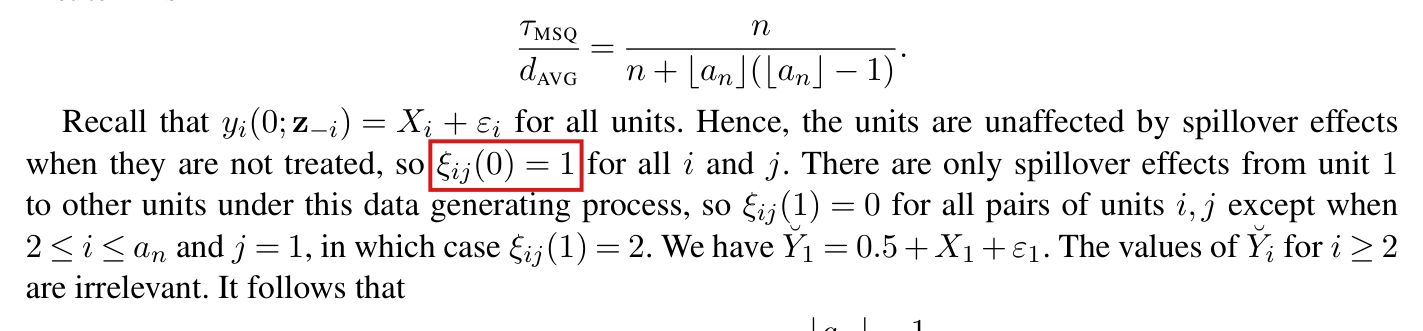
Corrected

“Of the units in Gi\mathcal{G}_i, some fraction will have bal⁡(Gj)=0\operatorname{bal}(G_j)=0. When we change ii's assignment, those units will change to bal⁡(Gj)=2\operatorname{bal}(G_j)=\colorbox{#ffe58a}{$2$}, and thus change the values of their outcomes. Similarly, some other fraction of Gi\mathcal{G}_i will have bal⁡(Gj)=−1\operatorname{bal}(G_j)=-1, and their values will change to bal⁡(Gj)=1\operatorname{bal}(G_j)=\colorbox{#ffe58a}{$1$}.”

Next paragraph: “… when we change ii's assignment from control to treatment and add two to bal⁡(Gj)\operatorname{bal}(G_j) for the units in Gi\mathcal{G}_i, a counteracting effect happens because we simultaneously change ℓ\ell's assignment from treatment to control and remove two from bal⁡(Gj)\operatorname{bal}(G_j) for units in Gℓ\mathcal{G}_\ell. The number of units that get two added to bal⁡(Gj)\operatorname{bal}(G_j) will, with high probability and relative to the sample size, be close to the number of units that get two removed …”

Crop of the paragraph that considers changing the assignment of a single unit i assigned to control under the Bernoulli design. A red box marks 'bal(G_j) = 1', the value said to follow from bal(G_j) = 0, and a second red box marks 'bal(G_j) = 0', the value said to follow from bal(G_j) = -1.
Supplement B, p. 6, paragraph beginning “To understand this behavior”. The marked values are those of bal⁡(Gj)\operatorname{bal}(G_j) after unit ii moves from control to treatment; they should be 22 and 11.
Crop of the paragraph on complete and paired randomization. Red boxes mark four phrases: 'add one' (to bal(G_j) for the units in script G_i), 'remove one' (from bal(G_j) for units in script G_l), 'one added' and 'one removed'.
Supplement B, p. 6, paragraph beginning “Now consider the same situation”. Each marked phrase states a change of one where the change is two.

Tables B1, B3, B5 and B7 of Supplement B report the absolute value of the Monte Carlo bias, and their captions should begin “Absolute bias”; every printed entry is unchanged.

Supplement B, captions of Tables B1, B3, B5 and B7, pp. 14, 16, 18 and 20 (the same PDF pages of Supplement B); replication files, make_stats_df.R

See also under Formal statements (Lean): P009-T25

As printed

Table B1, p. 14: “Bias of the HT and HÁ estimators with respect to EATE in the simulation study when the interference is contained within groups of units as described in Section 1.1.”

Table B3, p. 16: “Bias of the HT and HÁ estimators with respect to EATE when the interference structure is randomly generated using the unweighted balance function as described in Section 1.2.”

Table B5, p. 18: “Bias of the HT and HÁ estimators with respect to EATE when the interference structure is randomly generated using the weighted balance function as described in the end of Section 1.2.”

Table B7, p. 20: “Bias of the HT and HÁ estimators with respect to EATE when only one unit is interfering with other units as described in Section 1.3.”

Each table has the note “Note: Each cell presents the result from 50,000 draws from the data generating process.” In Tables B1 and B3, for both estimators and for n=102,103,104,105n=10^2,10^3,10^4,10^5, the row an=na_n=n reads 0.9970.997, 1.0001.000, 1.0001.000, 1.0001.000 under complete randomization and 0.9990.999, 1.0001.000, 1.0001.000, 1.0001.000 under paired randomization.

Replication files, make_stats_df.R:

get_bias <- function(res_mat) { abs(rowMeans(res_mat - 1)) }

The problem

The function that produces the entries takes the absolute value of the mean estimation error over the R=50,000R=50{,}000 draws, ∣R−1∑r=1R(τ^r−1)∣|R^{-1}\sum_{r=1}^R(\hat\tau_r-1)|. This is the size of the Monte Carlo bias without its sign, and the captions call it “Bias”. The difference matters most in the rows an=na_n=n under complete and paired randomization, where the entries near 11 correspond to a bias of −1-1. The printed magnitudes are correct, and the tables of nonnegative entries are naturally read as sizes of bias, which is the intended meaning.

Evidence an exact counterexample

The evidence is a check of the code and of the pages, a recalculation from the cached results, and an exact calculation. Regenerating the eight tables of bias and standard errors from the cached results in the replication files reproduces all 1,1041{,}104 printed cells at the printed precision. For the exact calculation, let an=na_n=n with nn even. Every assignment under complete or paired randomization has n/2n/2 treated units, every observed outcome equals its baseline Xi+εiX_i+\varepsilon_i, and both estimators equal (2/n)∑i=1n(2Zi−1)(Xi+εi)(2/n)\sum_{i=1}^n(2Z_i-1)(X_i+\varepsilon_i), whose expectation is 00. Since EATE is 11, the bias is −1-1 for every even nn. The cached results hold the magnitudes only, and the signs of the Monte Carlo biases of the original runs were not recovered.

What survives

All printed magnitudes, the tables of standard errors (B2, B4, B6 and B8), the root mean square errors and the figures are unaffected, and no conclusion of the paper uses the sign of these entries. The rows an=na_n=n lie outside the restricted-interference assumption, so a bias of −1-1 there does not contradict any proposition.

Corrected

Tables B1, B3, B5 and B7: “Absolute bias of the HT and HÁ estimators with respect to EATE …”, with the rest of each caption as printed. A common note may add: “Absolute bias is ∣R−1∑r=1R(τ^r−1)∣|R^{-1}\sum_{r=1}^R(\hat\tau_r-1)|, where R=50,000R=50{,}000.” The entries are unchanged.

Crop of the title 'Table B1' and its two-line caption. A red box marks the first word, 'Bias', of 'Bias of the HT and HA estimators with respect to EATE in the simulation study when the interference is contained within groups of units as described in Section 1.1'.
Supplement B, caption of Table B1, p. 14. The marked first word of the caption is “Bias”.
Crop of the lower part of Table B1. Red boxes mark the row labelled n at the end of Panel B, with entries 0.997, 1.000, 1.000, 1.000 for each estimator, and the row labelled n at the end of Panel C, with entries 0.999, 1.000, 1.000, 1.000 for each estimator. Below the table is the note 'Each cell presents the result from 50,000 draws from the data generating process'.
Supplement B, Table B1, p. 14: the last rows of Panel B (complete randomization), all of Panel C (paired randomization) and the note. The two marked rows, for an=na_n=n, have entries from 0.997 to 1.000.
Crop of the title 'Table B3' and its two-line caption. A red box marks the first word, 'Bias'.
Supplement B, caption of Table B3, p. 16. The marked first word is “Bias”.
Crop of the title 'Table B5' and its two-line caption. A red box marks the first word, 'Bias'.
Supplement B, caption of Table B5, p. 18. The marked first word is “Bias”.
Crop of the title 'Table B7' and its two-line caption. A red box marks the first word, 'Bias'.
Supplement B, caption of Table B7, p. 20. The marked first word is “Bias”.

The summary that the bias is negligible relative to the variance does not hold under complete interference (an=na_n=n) with complete or paired randomization, where both estimators have expectation 00 and EATE is 11; the sentence needs this exception.

Supplement B, p. 3, paragraph after Figure B1, last sentence; the rows concerned are an=na_n=n in Panels B and C of Tables B1–B4 (pp. 14–17)

See also under Formal statements (Lean): P009-T23, P009-T24

As printed

“The bias is negligible relative to the variance for the settings and sample sizes we consider here.”

Tables B1 and B3, row an=na_n=n, for n=102,103,104,105n=10^2,10^3,10^4,10^5 and for both estimators: bias 0.9970.997, 1.0001.000, 1.0001.000, 1.0001.000 in Panel B (complete randomization) and 0.9990.999, 1.0001.000, 1.0001.000, 1.0001.000 in Panel C (paired randomization). Tables B2 and B4, same row: standard error 0.4400.440, 0.1390.139, 0.0440.044, 0.0140.014 in Panel B and 0.4040.404, 0.1270.127, 0.0400.040, 0.0130.013 in Panel C.

The problem

The paragraph introduces the figures and the tables at the end of the supplement and summarizes “these results”. Its last sentence covers the rows an=na_n=n of the tables as well. In these rows, under complete and paired randomization, the tabulated bias is about one, which is the size of the estimand itself. From the rounded entries, it is more than twice the standard error at n=102n=10^2 and about 7171 and 7777 times the standard error at n=105n=10^5. The two estimators concentrate at 00 and not at τEATE=1\tau_{\mathrm{EATE}}=1. The low standard errors in these rows do not indicate accurate estimation. The tables print the bias in absolute value; its sign is the subject of P009-E025.

Evidence an exact counterexample

The evidence is a derivation from the data generating process on p. 2 of the supplement, together with the printed tables. Under complete interference Gi=U∖{i}G_i=\mathbf{U}\setminus\{i\}, and under either design exactly n/2n/2 units are treated. Substituting into the definition of the balance, I obtain

bal⁡(Gi)=∑j≠i(2Zj−1)=1−2Zi.\operatorname{bal}(G_i)=\sum_{j\ne i}(2Z_j-1)=1-2Z_i.

A treated unit has balance −1-1 and outcome Xi+εiX_i+\varepsilon_i. A control unit has balance +1+1 and outcome 2⋅0+Xi+εi2\cdot0+X_i+\varepsilon_i. Every observed outcome is Xi+εiX_i+\varepsilon_i, and both estimators equal (2/n)∑i(2Zi−1)(Xi+εi)(2/n)\sum_i(2Z_i-1)(X_i+\varepsilon_i), which has expectation zero because Pr⁡(Zi=1)=1/2\Pr(Z_i=1)=1/2 given the covariates. With the other assignments held fixed, the effect of unit ii's own treatment is 2(1−Zi)2(1-Z_i), which implies that τATE(Z)=1\tau_{\mathrm{ATE}}(\mathbf{Z})=1 and τEATE=1\tau_{\mathrm{EATE}}=1. The bias is exactly −1-1. The variance of the estimators is 58/(3n)58/(3n) under complete randomization and 49/(3n)+36/[n(n+1)(n+2)]49/(3n)+36/[n(n+1)(n+2)] under paired randomization. The root mean square error with respect to EATE then tends to one.

Row an=na_n=n: the printed bias (Tables B1 and B3) and standard error (Tables B2 and B4), and the standard deviation from the exact variance.
DesignnnPrinted biasPrinted standard errorExact standard deviation
Complete10210^20.9970.9970.4400.4400.43970.4397
Complete10310^31.0001.0000.1390.1390.13900.1390
Complete10410^41.0001.0000.0440.0440.04400.0440
Complete10510^51.0001.0000.0140.0140.01390.0139
Paired10210^20.9990.9990.4040.4040.40420.4042
Paired10310^31.0001.0000.1270.1270.12780.1278
Paired10410^41.0001.0000.0400.0400.04040.0404
Paired10510^51.0001.0000.0130.0130.01280.0128

In every other row of Tables B1–B8 the rounded bias is less than a tenth of the rounded standard error; the largest ratio is 0.0990.099.

What survives

The tabulated bias and standard errors in these rows need no correction, and Figures B2 and B3 do not show an=na_n=n. The statement on p. 6 that the outcomes and the standard error are unchanged in this case is also correct, although it does not mention the bias. No result of the article is contradicted. Here dAVG=nd_{\mathrm{AVG}}=n and Assumption 2 fails, and the article itself has a related example on p. 684. Only the scope of the summary sentence changes.

Corrected

“The bias is negligible relative to the variance for the settings and sample sizes we consider here, except under complete interference with the unweighted balance function and complete or paired randomization. In that exception, both estimators have expectation zero while EATE is one, so their signed bias is −1-1.”

A sentence may also be added to the paragraph on p. 6 that begins “The extreme case”: “Despite the unchanged standard error, in this extreme case both estimators are centered at zero rather than at EATE.”

Crop of the paragraph beginning 'The primary focus in the simulations is the root mean square error (RMSE) of the Hajek estimator'. A red box marks its last sentence: 'The bias is negligible relative to the variance for the settings and sample sizes we consider here.'
Supplement B, p. 3, the paragraph after Figure B1. The marked sentence covers every setting in the figures and tables that the paragraph introduces.
Crop of Panel B of Table B1, with the bias of the Horvitz-Thompson and Hajek estimators for n = 100, 1000, 10000 and 100000 and six sequences a_n. In the rows for a_n = 1, 25, 8 n^0.25, 2.5 n^0.5 and 0.25 n the entries are at most 0.041. A red box marks the last row, a_n = n, with entries 0.997, 1.000, 1.000, 1.000 for each estimator.
Supplement B, p. 14: Panel B (complete randomization) of Table B1. In the marked row an=na_n=n the bias of both estimators is 0.9970.997 or 1.0001.000, and the estimand is τEATE=1\tau_{\mathrm{EATE}}=1. Panel C and Table B3 have the same pattern.

In the illustration of Section 1.4 of Supplement B, the spillover effect on an untreated unit is ξij(0)=0\xi_{ij}(0)=0, not 11.

Supplement B, Section 1.4, p. 8 (PDF p. 8 of Supplement B), paragraph beginning “Recall that”

See also under Formal statements (Lean): P009-T33

As printed

“Recall that yi(0;z−i)=Xi+εiy_i(0;\mathbf{z}_{-i})=X_i+\varepsilon_i for all units. Hence, the units are unaffected by spillover effects when they are not treated, so ξij(0)=1\xi_{ij}(0)=\colorbox{#ffe58a}{$1$} for all ii and jj.”

The problem

The sentence states the reason for the value zero and prints the value one. The article defines ξij(z)\xi_{ij}(z) on p. 690, for distinct units ii and jj, as the spillover effect from unit jj to unit ii when the treatment of unit ii is held at zz. If an untreated unit is unaffected by the treatments of the other units, then this effect is zero.

Evidence a derivation

The evidence is a derivation from the definition and a check of the page. In the illustration, the two potential outcomes whose difference defines ξij(0)\xi_{ij}(0) both equal Xi+εiX_i+\varepsilon_i, and their difference is identically zero. The display for B1B_1 that follows the sentence is the one obtained with ξij(0)=0\xi_{ij}(0)=0: each of its ⌊an⌋−1\lfloor a_n\rfloor-1 nonzero summands equals 2Y˘1⋅2=2+4X1+4ε12\breve{Y}_1\cdot 2=2+4X_1+4\varepsilon_1.

What survives

This correction leaves the printed expression for B1B_1 unchanged: it already uses the value zero.

Corrected

“Hence, the units are unaffected by spillover effects when they are not treated, so ξij(0)=0\xi_{ij}(0)=\colorbox{#ffe58a}{$0$} for all distinct ii and jj.”

Crop of five lines of text between two displays. A red box marks the words 'xi i j of 0 equals 1' in the sentence 'Hence, the units are unaffected by spillover effects when they are not treated, so xi i j of 0 equals 1 for all i and j'.
Supplement B, Section 1.4, p. 8. The marked value of ξij(0)\xi_{ij}(0) is printed as 1.

In the illustration of Section 1.4 of Supplement B, with b=⌊an⌋b=\lfloor a_n\rfloor, the term B2B_2 equals (b−1)(b−2)/{n+b(b−1)}(b-1)(b-2)/\{n+b(b-1)\}, not b(b−1)/{n+b(b−1)}b(b-1)/\{n+b(b-1)\}, and the right side of the displayed limit becomes {n−(b−1)2}/{n+b(b−1)}\{n-(b-1)^2\}/\{n+b(b-1)\}; the three limiting regimes are unchanged.

Supplement B, Section 1.4, p. 8 (PDF p. 8 of Supplement B), display after “It follows that” and display after “Taken together, we can conclude that”

See also under Formal statements (Lean): P009-T21, P009-T22

As printed

“Taken together, we have

B2=1ndAVG∑i=2⌊an⌋∑j=2⌊an⌋1[i≠j]Cov⁡(Yi,Yj∣Zi=1,Zj=1)B_2=\frac{1}{nd_{\mathrm{AVG}}}\sum_{i=2}^{\lfloor a_n\rfloor}\sum_{j=2}^{\lfloor a_n\rfloor}\mathbf{1}[i\ne j]\operatorname{Cov}\bigl(Y_i,Y_j\mid Z_i=1,Z_j=1\bigr)

Conditional on Zi=1Z_i=1, we have Yi=2Z1+Xi+εiY_i=2Z_1+X_i+\varepsilon_i for all 2≤i≤an2\le i\le a_n. Hence, for all 2≤i≠j≤an2\le i\ne j\le a_n,

Cov⁡(Yi,Yj∣Zi=1,Zj=1)=4Var⁡(Z1)=1.\operatorname{Cov}\bigl(Y_i,Y_j\mid Z_i=1,Z_j=1\bigr)=4\operatorname{Var}(Z_1)=1.

It follows that

B2=⌊an⌋(⌊an⌋−1)n+⌊an⌋(⌊an⌋−1).B_2=\frac{\colorbox{#ffe58a}{$\displaystyle \lfloor a_n\rfloor\bigl(\lfloor a_n\rfloor-1\bigr)$}}{n+\lfloor a_n\rfloor\bigl(\lfloor a_n\rfloor-1\bigr)}.

… Taken together, we can conclude that

ndAVG−1[Var⁡^BER(τ^HT)−Var⁡(τ^HT)]→pn−(⌊an⌋−1)−⌊an⌋(⌊an⌋−1)n+⌊an⌋(⌊an⌋−1).”nd_{\mathrm{AVG}}^{-1}\Bigl[\widehat{\operatorname{Var}}_{\mathrm{BER}}(\hat\tau_{\mathrm{HT}})-\operatorname{Var}(\hat\tau_{\mathrm{HT}})\Bigr]\xrightarrow{p}\frac{n-\bigl(\lfloor a_n\rfloor-1\bigr)-\colorbox{#ffe58a}{$\displaystyle \lfloor a_n\rfloor\bigl(\lfloor a_n\rfloor-1\bigr)$}}{n+\lfloor a_n\rfloor(\lfloor a_n\rfloor-1)}.\text{''}
The problem

Let b=⌊an⌋b=\lfloor a_n\rfloor. The double sum runs over the ordered pairs (i,j)(i,j) such that 2≤i≠j≤b2\le i\ne j\le b. There are b−1b-1 such indices and (b−1)(b−2)(b-1)(b-2) such ordered pairs, and each covariance equals one. The printed numerator b(b−1)b(b-1) is the number of ordered pairs of distinct indices among 1,…,b1,\ldots,b, which includes unit 1, although the supplement notes a few lines earlier that the covariance is zero whenever i=1i=1 or j=1j=1. The printed value of B2B_2 is too large by 2(b−1)/{n+b(b−1)}2(b-1)/\{n+b(b-1)\}, and the same excess enters the last term of the numerator in the displayed limit.

The excess is at most n−1/2n^{-1/2}. The displayed limit keeps nn on its right side and is read as the statement that the difference of the two sides tends to zero in probability. In that sense it remains true, and the three regimes discussed after it are unchanged. What is wrong is the exact value of B2B_2 and, with it, the exact value of the normalized expected difference ndAVG−1{E[Var⁡^BER(τ^HT)]−Var⁡(τ^HT)}nd_{\mathrm{AVG}}^{-1}\{\mathbb{E}[\widehat{\operatorname{Var}}_{\mathrm{BER}}(\hat\tau_{\mathrm{HT}})]-\operatorname{Var}(\hat\tau_{\mathrm{HT}})\} at a finite sample size.

Evidence an exact counterexample

The evidence is a count, a direct derivation and an exact enumeration. Let m=b−1m=b-1 and D=ndAVG=n+b(b−1)D=nd_{\mathrm{AVG}}=n+b(b-1). The count gives B2=m(m−1)/DB_2=m(m-1)/D. Under X1+ε1=−1/4X_1+\varepsilon_1=-1/4, the supplement’s values B1=m/DB_1=m/D and τMSQ=1\tau_{\mathrm{MSQ}}=1 are correct, and the right side in Proposition 7 is

τMSQdAVG−B1−B2=n−m−m(m−1)D=n−m2D.\frac{\tau_{\mathrm{MSQ}}}{d_{\mathrm{AVG}}}-B_1-B_2=\frac{n-m-m(m-1)}{D}=\frac{n-m^2}{D}.

A direct computation of Var⁡(τ^HT)\operatorname{Var}(\hat\tau_{\mathrm{HT}}) and of E[Var⁡^BER(τ^HT)]\mathbb{E}[\widehat{\operatorname{Var}}_{\mathrm{BER}}(\hat\tau_{\mathrm{HT}})] under independent assignments with probability 1/21/2, which does not use Proposition 7, gives

ndAVG{E[Var⁡^BER(τ^HT)]−Var⁡(τ^HT)}=n−2m{1+2(X1+ε1)}−m(m−1)D,\frac{n}{d_{\mathrm{AVG}}}\Bigl\{\mathbb{E}\bigl[\widehat{\operatorname{Var}}_{\mathrm{BER}}(\hat\tau_{\mathrm{HT}})\bigr]-\operatorname{Var}(\hat\tau_{\mathrm{HT}})\Bigr\}=\frac{n-2m\{1+2(X_1+\varepsilon_1)\}-m(m-1)}{D},

which equals (n−m2)/D(n-m^2)/D when X1+ε1=−1/4X_1+\varepsilon_1=-1/4.

For n=6n=6, b=4b=4, X1+ε1=−1/4X_1+\varepsilon_1=-1/4 and Xi+εi=1X_i+\varepsilon_i=1 for i≥2i\ge2, enumerating the 6464 assignments in rational arithmetic, I find D=18D=18, B1=1/6B_1=1/6, B2=1/3B_2=1/3, E[Var⁡^BER(τ^HT)]=229/144\mathbb{E}[\widehat{\operatorname{Var}}_{\mathrm{BER}}(\hat\tau_{\mathrm{HT}})]=229/144 and Var⁡(τ^HT)=241/144\operatorname{Var}(\hat\tau_{\mathrm{HT}})=241/144. The normalized expected difference is −1/6-1/6. According to the printed formulas, B2=2/3B_2=2/3 and the right side is −1/2-1/2. The same enumeration for every 1≤b≤n≤81\le b\le n\le 8 (3636 cases) agrees with the corrected formulas. Four of these cases are shown below.

Printed and exact values in the illustration, with X1+ε1=−1/4X_1+\varepsilon_1=-1/4 and Xi+εi=1X_i+\varepsilon_i=1 for i≥2i\ge2.
nnbbB2B_2, printedB2B_2, exactright side of the limit, printednormalized expected difference, exact
55336/116/112/112/11−3/11-3/111/111/11
66442/32/31/31/3−1/2-1/2−1/6-1/6
88555/75/73/73/7−4/7-4/7−2/7-2/7
88887/87/821/3221/32−55/64-55/64−41/64-41/64

The corrected right side exceeds the printed one by δn=2m/D\delta_n=2m/D. The identity D2−4nm2=(n−m2)2+2nm+2m3+m2D^2-4nm^2=(n-m^2)^2+2nm+2m^3+m^2 implies that D2≥4nm2D^2\ge4nm^2, and I conclude that 0≤δn≤n−1/20\le\delta_n\le n^{-1/2} for all nn and all 1≤b≤n1\le b\le n.

What survives

The three limits are unchanged: one when an=o(n0.5)a_n=o(n^{0.5}), minus one when n=o(an2)n=o(a_n^2), and (1−c2)/(1+c2)(1-c^2)/(1+c^2) when an/n0.5a_n/n^{0.5} tends to c>0c>0. The displayed limit also remains true in the sense above, since its right side differs from the corrected one by at most n−1/2n^{-1/2}. Proposition 7 defines B2B_2 by the correct sum, and its proof does not use this illustration. The simulation code excludes unit 1 from the units that unit 1 affects and does not use the closed form for B2B_2. The reported bias, standard errors and root mean square errors do not depend on the count. At a finite sample size the sign of the normalized expected difference can differ from the sign of the printed right side, as in the first row of the table.

Corrected

Let b=⌊an⌋b=\lfloor a_n\rfloor, and let the assignments be independent with probability 1/21/2, as in the supplement’s calculation. The units affected by the treatment of unit 1 are 2,…,b2,\ldots,b, which gives (b−1)(b−2)(b-1)(b-2) ordered pairs of distinct units. It follows that

B2=(b−1)(b−2)n+b(b−1).B_2=\frac{\colorbox{#ffe58a}{$\displaystyle (b-1)(b-2)$}}{n+b(b-1)}.

Under X1+ε1=−1/4X_1+\varepsilon_1=-1/4, B1=(b−1)/{n+b(b−1)}B_1=(b-1)/\{n+b(b-1)\} as printed, and

τMSQdAVG−B1−B2=n−(b−1)−(b−1)(b−2)n+b(b−1)=n−(b−1)2n+b(b−1).\frac{\tau_{\mathrm{MSQ}}}{d_{\mathrm{AVG}}}-B_1-B_2=\frac{n-(b-1)-\colorbox{#ffe58a}{$\displaystyle (b-1)(b-2)$}}{n+b(b-1)}=\frac{n-(b-1)^2}{n+b(b-1)}.

For every nn and every 1≤b≤n1\le b\le n, this is the exact value of ndAVG−1{E[Var⁡^BER(τ^HT)]−Var⁡(τ^HT)}nd_{\mathrm{AVG}}^{-1}\{\mathbb{E}[\widehat{\operatorname{Var}}_{\mathrm{BER}}(\hat\tau_{\mathrm{HT}})]-\operatorname{Var}(\hat\tau_{\mathrm{HT}})\}. Taken together,

ndAVG−1[Var⁡^BER(τ^HT)−Var⁡(τ^HT)]−n−(b−1)2n+b(b−1)→p0.nd_{\mathrm{AVG}}^{-1}\Bigl[\widehat{\operatorname{Var}}_{\mathrm{BER}}(\hat\tau_{\mathrm{HT}})-\operatorname{Var}(\hat\tau_{\mathrm{HT}})\Bigr]-\frac{n-\colorbox{#ffe58a}{$\displaystyle (b-1)^2$}}{n+b(b-1)}\xrightarrow{p}0.

The printed right side differs from this one by 2(b−1)/{n+b(b−1)}≤n−1/22(b-1)/\{n+b(b-1)\}\le n^{-1/2}, so the printed display is also true in this sense, and the three regimes are as printed.

Crop from the display of B 2 as a double sum over i and j from 2 to floor of a n, through the display of B 1. A red box marks the numerator, floor of a n times floor of a n minus 1, of the fraction printed for B 2 after the words 'It follows that'.
Supplement B, Section 1.4, p. 8. The double sum for B2B_2 starts at 2 in both indices; the marked numerator of the closed form counts ⌊an⌋(⌊an⌋−1)\lfloor a_n\rfloor(\lfloor a_n\rfloor-1) pairs.
Crop of the display that states the limit in probability of the normalized difference between the variance estimator and the variance. A red box marks the last term of the numerator on the right side, floor of a n times floor of a n minus 1.
Supplement B, Section 1.4, p. 8, display after “Taken together, we can conclude that”. The marked term of the numerator carries the same count.

“Compilers and noncompilers” should read “compliers and noncompliers”.

Section 2, p. 675 (PDF p. 3), paragraph beginning “Previous investigations”, sentence on Sobel (2006)

As printed

“Sobel (2006) derives the expectation of an instrumental variables estimator used in housing mobility experiments under unknown interference, and he shows that it is a mixture of primary and spillover effects for compilers and noncompilers.”

The problem

The sentence describes an instrumental variables estimator, whose two compliance groups are the compliers and the noncompliers. Both words are misspelled.

Evidence a check of the printed page

I checked the spelling only and did not compare the sentence with Sobel (2006).

What survives

Nothing else is affected.

Corrected

“… and he shows that it is a mixture of primary and spillover effects for compliers and noncompliers.”

Crop of the paragraph beginning 'Previous investigations under unknown interference'. A red box marks the words 'compilers and noncompilers' at the end of the sentence on Sobel (2006).
Section 2, p. 675 (PDF p. 3), the sentence on Sobel (2006). The marked words are the misprint.

The constant 2k22k^2 in the last step of the proof of Lemma A17 does not follow from Lemma A4, which gives 4k24k^2 for the two terms; the bound holds by a direct argument under paired randomization.

Supplement A, p. 17 (PDF p. 17 of the supplement), proof of Lemma A17, last line of the final display and the sentence after it

See also under Formal statements (Lean): P009-T34, P009-T44

As printed
=1n∑i=1nIρ(i)i∑z=01∣E[yi(z;Z~−i)∣Zi=z]−E[yi(z;Z~−i)]∣≤2k2n∑i=1nIρ(i)i=2k2n−1RSUM.\begin{aligned} &= \frac{1}{n}\sum_{i=1}^n I_{\rho(i)i}\sum_{z=0}^1 \Bigl|\mathrm{E}[y_i(z;\widetilde{\mathbf{Z}}_{-i}) \mid Z_i = z] - \mathrm{E}[y_i(z;\widetilde{\mathbf{Z}}_{-i})]\Bigr| \\ &\leq \frac{2k^2}{n}\sum_{i=1}^n I_{\rho(i)i} = 2k^2 n^{-1} R_{\mathrm{SUM}}. \end{aligned}

where the second to last inequality follows from Lemma A4.

The problem

Lemma A4 (Supplement A, p. 3) bounds ∣E[yi(z;Z−i)∣Zi=z]−E[yi(z;Z−i)]∣|\mathrm{E}[y_i(z;\mathbf{Z}_{-i}) \mid Z_i = z] - \mathrm{E}[y_i(z;\mathbf{Z}_{-i})]| by 2k22k^2 for a single value of zz. The inner sum in the display has two terms, z=0z = 0 and z=1z = 1. Applying the lemma to each term, I obtain 4k24k^2 and not the printed 2k22k^2. The parallel step in the proof of Lemma A14 (Supplement A, p. 14) applies Lemma A4 in the same way and carries the factor 4k24k^2. The step in question is also the last inequality of the display, not the second to last. The printed bound is nevertheless correct, because under paired randomization each of the two differences is at most kk.

Evidence a derivation

The evidence is a derivation. Fix ii and zz, and let gz=yi(z;Z~−i)g_z = y_i(z;\widetilde{\mathbf{Z}}_{-i}). Since Pr⁡(Zi=z)=1/2\Pr(Z_i = z) = 1/2 under paired randomization, E[gz]\mathrm{E}[g_z] is the average of E[gz∣Zi=z]\mathrm{E}[g_z \mid Z_i = z] and E[gz∣Zi=1−z]\mathrm{E}[g_z \mid Z_i = 1 - z], and I have

∣E[gz∣Zi=z]−E[gz]∣=12∣E[gz∣Zi=z]−E[gz∣Zi=1−z]∣≤12(E[∣gz∣∣Zi=z]+E[∣gz∣∣Zi=1−z])=E∣gz∣≤k.\begin{aligned} \bigl|\mathrm{E}[g_z \mid Z_i = z] - \mathrm{E}[g_z]\bigr| &= \frac{1}{2}\bigl|\mathrm{E}[g_z \mid Z_i = z] - \mathrm{E}[g_z \mid Z_i = 1 - z]\bigr| \\ &\leq \frac{1}{2}\bigl(\mathrm{E}[|g_z| \mid Z_i = z] + \mathrm{E}[|g_z| \mid Z_i = 1 - z]\bigr) = \mathrm{E}|g_z| \leq k. \end{aligned}

In the last inequality, I used Assumption 1C, with Jensen’s inequality since s≥1s \geq 1. Summing over z∈{0,1}z \in \{0, 1\}, I find that the inner sum is at most 2k2k, and 2k≤2k22k \leq 2k^2 because Assumption 1A forces k≥2k \geq 2. The terms with Iρ(i)i=0I_{\rho(i)i} = 0 vanish, as the printed proof shows.

What survives

Lemma A17 holds as stated, with its constant, and Proposition 4 uses only the order n−1RSUMn^{-1}R_{\mathrm{SUM}}. Only the justification of the last step changes.

Corrected
=1n∑i=1nIρ(i)i∑z=01∣E[yi(z;Z~−i)∣Zi=z]−E[yi(z;Z~−i)]∣≤2k2n∑i=1nIρ(i)i=2k2n−1RSUM,\begin{aligned} &= \frac{1}{n}\sum_{i=1}^n I_{\rho(i)i}\sum_{z=0}^1 \Bigl|\mathrm{E}[y_i(z;\widetilde{\mathbf{Z}}_{-i}) \mid Z_i = z] - \mathrm{E}[y_i(z;\widetilde{\mathbf{Z}}_{-i})]\Bigr| \\ &\leq \frac{2k^2}{n}\sum_{i=1}^n I_{\rho(i)i} = 2k^2 n^{-1} R_{\mathrm{SUM}}, \end{aligned}

where the last inequality holds because paired randomization has Pr⁡(Zi=z)=1/2\Pr(Z_i = z) = 1/2: each absolute difference is then at most E∣yi(z;Z~−i)∣≤k\mathrm{E}|y_i(z;\widetilde{\mathbf{Z}}_{-i})| \leq k by Assumption 1C, and the inner sum is at most 2k≤2k22k \leq 2k^2.

Crop of the last two lines of a displayed chain and the sentence after it. The first line reads: equals one over n times the sum over i of I sub rho(i) i times the sum over z from 0 to 1 of the absolute value of E of y i of (z; Z-tilde minus i) given Z i = z, minus E of y i of (z; Z-tilde minus i). The second line reads: is at most 2 k squared over n times the sum over i of I sub rho(i) i, which equals 2 k squared n to the minus 1 R SUM. A red outline surrounds the symbols is at most 2 k squared over n. The sentence below reads: where the second to last inequality follows from Lemma A4, and a second red outline surrounds it. The crop ends with the statement of Lemma A18.
Supplement A, p. 17, end of the proof of Lemma A17. The outlines mark the constant 2k22k^2 in the last line of the display and the sentence that attributes the step to Lemma A4.

Clarity notes

Imprecise or ambiguous wording whose intended meaning is correct; not an error.

Two units that are interference dependent in the sense of Definition 5 may have dependent outcomes under a Bernoulli design, but need not; the proofs use only the converse, that units with dij=0d_{ij}=0 have independent outcomes.

Section 5.2.1, p. 684 (PDF p. 12), first paragraph

As printed

“The outcomes of any two units are independent under a Bernoulli design when the no-interference assumption holds. This is not the case when units interfere. A single treatment may then affect two or more units, and the corresponding outcomes are dependent. That is, two units' outcomes are dependent when they are interference dependent according to Definition 5.”

Intended meaning

Definition 5 sets dij=1d_{ij}=1 when the treatment of some unit can affect both unit ii and unit jj, and the paragraph uses the definition to mark where dependence between outcomes can occur. Under a Bernoulli design, if dij=0d_{ij}=0, then the outcomes of units ii and jj are functions of disjoint sets of independent treatments, and they are independent. This is the direction that the variance bound behind Proposition 2 uses (Lemma A9 of Supplement A), and it is correct. The printed sentences state the other direction, which does not hold in general. For example, let Z1Z_1, Z2Z_2 and Z3Z_3 be independent with probability 1/21/2, and let y1(z)=z3y_1(\mathbf{z})=z_3, y3(z)=z3y_3(\mathbf{z})=z_3 and y2(z)=z2+z3−2z2z3y_2(\mathbf{z})=z_2+z_3-2z_2z_3, which is the sum of z2z_2 and z3z_3 modulo 22. Since the treatment of unit 3 can change both Y1Y_1 and Y2Y_2, I have d12=1d_{12}=1. Each of the four values of (Y1,Y2)(Y_1,Y_2) has probability 1/41/4, and the two outcomes are independent.

Corrected

“A single treatment may then affect two or more units, and the corresponding outcomes may be dependent. That is, two units' outcomes may be dependent when they are interference dependent according to Definition 5.”

Crop of the six-line paragraph that opens the page. Red boxes mark the words 'are dependent' in 'the corresponding outcomes are dependent' and in 'two units' outcomes are dependent when they are interference dependent according to Definition 5'.
Section 5.2.1, p. 684 (PDF p. 12), first paragraph. The two marked phrases state dependence as a fact.

In Definition 9, the “maximum values of qq and ss” are taken with the constant kk of Assumption 1 held fixed, and they are infinite when the corresponding outcomes are bounded by that same kk, in which case the exponents (q−2)/q(q-2)/q and (s−1)/s(s-1)/s are read as 11.

Definition 9, p. 687 (PDF p. 15); Supplement A, proofs of Lemmas A20, A22 and A23, pp. 21 and 23

See also under Formal statements (Lean): P009-T26, P009-T45, P009-T46

As printed

“Definition 9 (External and internal average mixing coefficients). For the maximum values of qq and ss such that Assumptions 1B and 1C hold, let

αEXT=1n∑i=1n∑j=1n(1−dij)[α(Z~i,Z~j)]q−2qandαINT=∑i=1n[α(Zi,Z~−i)]s−1s,\alpha_{\mathrm{EXT}}=\frac{1}{n}\sum_{i=1}^n\sum_{j=1}^n(1-d_{ij})\bigl[\alpha(\widetilde{\mathbf{Z}}_i,\widetilde{\mathbf{Z}}_j)\bigr]^{\frac{q-2}{q}}\quad\text{and}\quad\alpha_{\mathrm{INT}}=\sum_{i=1}^n\bigl[\alpha(Z_i,\widetilde{\mathbf{Z}}_{-i})\bigr]^{\frac{s-1}{s}},

where 000^0 is defined as zero to accommodate the cases q=2q=2 and s=1s=1.”

Intended meaning

Assumption 1 asks for constants k<∞k<\infty, q≥2q\ge2 and s≥1s\ge1 such that the moment bounds of Assumptions 1B and 1C hold for all units in the sequence of samples, and Definition 9 then takes the maximum values of qq and ss. If this is read as a request for the largest finite exponents, the definition selects nothing when the potential outcomes are bounded: if every potential outcome equals 11 and k=2k=2, then every finite q≥2q\ge2 and s≥1s\ge1 is admissible. The discussion after Assumption 1 on p. 682 covers this case: bounded potential outcomes correspond “to the case where Assumption 1 holds as q→∞q\to\infty and s→∞s\to\infty”. The intended reading keeps the constant kk of Assumption 1 fixed, takes the largest admissible exponents, and allows the value infinity, with (q−2)/q(q-2)/q and (s−1)/s(s-1)/s read as their limit 11.

With this reading the definition is complete. For a fixed kk, a finite supremum of the admissible exponents is attained, because at each sample size the outcomes take finitely many values and each moment is continuous in the exponent. If the admissible exponents are unbounded, then the outcomes are bounded by kk, and the bounds of Lemmas A20 and A22 hold with exponent 11 in the limit. A finite supremum that is not attained can occur only if the constant kk is allowed to change with the exponent, and Assumption 1 does not state that. The rates of Propositions 5 and 6 are unchanged.

Corrected

“Definition 9 (External and internal average mixing coefficients). Let kk be a constant for which Assumption 1 holds, and let qq and ss be the largest values, possibly infinite, such that Assumptions 1B and 1C hold with this kk. Let

αEXT=1n∑i=1n∑j=1n(1−dij)[α(Z~i,Z~j)]q−2qandαINT=∑i=1n[α(Zi,Z~−i)]s−1s,\alpha_{\mathrm{EXT}}=\frac{1}{n}\sum_{i=1}^n\sum_{j=1}^n(1-d_{ij})\bigl[\alpha(\widetilde{\mathbf{Z}}_i,\widetilde{\mathbf{Z}}_j)\bigr]^{\frac{q-2}{q}}\quad\text{and}\quad\alpha_{\mathrm{INT}}=\sum_{i=1}^n\bigl[\alpha(Z_i,\widetilde{\mathbf{Z}}_{-i})\bigr]^{\frac{s-1}{s}},

where 000^0 is defined as zero to accommodate the cases q=2q=2 and s=1s=1, and where (q−2)/q(q-2)/q and (s−1)/s(s-1)/s are read as 11 when qq or ss is infinite.”

The same convention applies where Supplement A sets ss or qq to its maximum value, in the proofs of Lemmas A20, A22 and A23. An alternative is to fix any admissible q≥2q\ge2 and s≥1s\ge1 with a common finite kk, to define the coefficients for those exponents, and to state Assumptions 5 and 6 and the rates with the same choices.

Crop of four lines of text, Definition 9 with its display of alpha EXT and alpha INT, and the line after the display. Red boxes mark the words 'maximum' at the end of one line and 'values of q and s' at the start of the next.
Definition 9, p. 687 (PDF p. 15). The marked words ask for the maximum values of qq and ss.

Lemma A6 writes its bound as Op\mathcal{O}_{\mathrm{p}} of the signed sum of two random errors; the bound that the proof gives, and that the later lemmas use, has the sum of their absolute values.

Supplement A, Lemma A6, p. 4 (statement) and p. 5 (end of the proof)

As printed

Lemma A6, p. 4: “If μ^z−μ˘z=op(1)\hat\mu_z-\breve\mu_z=o_{\mathrm{p}}(1) and n^z/n−1=op(1)\hat n_z/n-1=o_{\mathrm{p}}(1), then:”

nn^zμ^z−μ˘z=Op((μ^z−μ˘z)+(n^z/n−1)).\frac{n}{\hat n_z}\hat\mu_z-\breve\mu_z=\mathcal{O}_{\mathrm{p}}\big(\colorbox{#ffe58a}{$\displaystyle (\hat\mu_z-\breve\mu_z)+(\hat n_z/n-1)$}\big).

End of the proof, p. 5:

nn^zμ^z−μ˘z=(μ^z−μ˘z)−(n^z/n−1)μ˘z+r1−r2,\frac{n}{\hat n_z}\hat\mu_z-\breve\mu_z=(\hat\mu_z-\breve\mu_z)-(\hat n_z/n-1)\breve\mu_z+r_1-r_2,

“where r1=op((μ^z−μ˘z)+(n^z/n−1))r_1=o_{\mathrm{p}}\big(\colorbox{#ffe58a}{$(\hat\mu_z-\breve\mu_z)+(\hat n_z/n-1)$}\big) and r2=op((n^z/n−1)(μ˘z+1))r_2=o_{\mathrm{p}}\big(\colorbox{#ffe58a}{$(\hat n_z/n-1)(\breve\mu_z+1)$}\big) since μ^z−μ˘z\hat\mu_z-\breve\mu_z converges in probability to zero and n^z/n\hat n_z/n converges to one. The bound ∣μ˘z∣≤k2|\breve\mu_z|\le k^2 completes the proof.”

Intended meaning

The lemma transfers the rates of the two errors to the ratio, and the display is shorthand for a bound by their magnitudes. Let A=μ^z−μ˘zA=\hat\mu_z-\breve\mu_z, B=n^z/n−1B=\hat n_z/n-1 and D=(n/n^z)μ^z−μ˘zD=(n/\hat n_z)\hat\mu_z-\breve\mu_z. By the identity on p. 4 of the supplement, I have

D=A−μ˘zB1+B.D=\frac{A-\breve\mu_zB}{1+B}.

Since B=op(1)B=o_{\mathrm{p}}(1), the event {∣B∣≤1/2}\{|B|\le1/2\} has probability tending to one. On this event, using the bound ∣μ˘z∣≤k2|\breve\mu_z|\le k^2, I obtain ∣D∣≤2(∣A∣+k2∣B∣)≤2max⁡(1,k2)(∣A∣+∣B∣)|D|\le2(|A|+k^2|B|)\le2\max(1,k^2)(|A|+|B|), which implies that D=Op(∣A∣+∣B∣)D=\mathcal{O}_{\mathrm{p}}(|A|+|B|). Lemmas A10 and A23 apply the lemma with deterministic rates for AA and BB, and this bound gives the rates stated there.

The absolute values are needed, because the signed sum can vanish when DD does not. For example, let n=3rn=3r with rr odd, and let independent blocks of three units receive the assignments (1,0,0)(1,0,0) or (0,1,1)(0,1,1) with probability 1/21/2 each. Let the outcomes be fixed at (1,0,0)(1,0,0) in every block. In this design there is no interference, and every treatment probability is 1/21/2. Let z=1z=1, and let KK denote the number of blocks that receive (0,1,1)(0,1,1). Then A=(r−2K)/(3r)=−BA=(r-2K)/(3r)=-B, and A+B=0A+B=0 for every assignment, while D=2(r−2K)/(3(r+K))≠0D=2(r-2K)/(3(r+K))\ne0 and E[A2]=E[B2]=1/(9r)\mathrm{E}[A^2]=\mathrm{E}[B^2]=1/(9r). In the same example I find r1=B2/(1+B)>0r_1=B^2/(1+B)>0, and the scale printed for r1r_1 needs absolute values as well.

Corrected

Lemma A6: “If μ^z−μ˘z=op(1)\hat\mu_z-\breve\mu_z=o_{\mathrm{p}}(1) and n^z/n−1=op(1)\hat n_z/n-1=o_{\mathrm{p}}(1), then:”

nn^zμ^z−μ˘z=Op(∣μ^z−μ˘z∣+∣n^z/n−1∣).\frac{n}{\hat n_z}\hat\mu_z-\breve\mu_z=\mathcal{O}_{\mathrm{p}}\big(\colorbox{#ffe58a}{$\displaystyle |\hat\mu_z-\breve\mu_z|+|\hat n_z/n-1|$}\big).

Here Dn=Op(Tn)D_n=\mathcal{O}_{\mathrm{p}}(T_n) for nonnegative random variables TnT_n means that for every ε>0\varepsilon>0 there exist finite MM and NN such that Pr⁡(∣Dn∣>MTn)≤ε\Pr(|D_n|>MT_n)\le\varepsilon for all n≥Nn\ge N. The lemma holds under Assumption 1, which enters through the bound ∣μ˘z∣≤k2|\breve\mu_z|\le k^2. In the proof, r1=op(∣μ^z−μ˘z∣+∣n^z/n−1∣)r_1=o_{\mathrm{p}}\big(\colorbox{#ffe58a}{$|\hat\mu_z-\breve\mu_z|+|\hat n_z/n-1|$}\big) and r2=op(∣n^z/n−1∣(∣μ˘z∣+1))r_2=o_{\mathrm{p}}\big(\colorbox{#ffe58a}{$|\hat n_z/n-1|(|\breve\mu_z|+1)$}\big).

The form used in Lemmas A10 and A23 follows: if in addition μ^z−μ˘z=Op(an)\hat\mu_z-\breve\mu_z=\mathcal{O}_{\mathrm{p}}(a_n) and n^z/n−1=Op(bn)\hat n_z/n-1=\mathcal{O}_{\mathrm{p}}(b_n) for positive deterministic sequences (an)(a_n) and (bn)(b_n), then (n/n^z)μ^z−μ˘z=Op(an+bn)(n/\hat n_z)\hat\mu_z-\breve\mu_z=\mathcal{O}_{\mathrm{p}}(a_n+b_n).

Crop of Lemma A6: if mu-hat_z minus mu-breve_z is o_p(1) and n-hat_z over n minus 1 is o_p(1), then (n over n-hat_z) mu-hat_z minus mu-breve_z equals O_p of a sum. A red box marks the sum (mu-hat_z minus mu-breve_z) + (n-hat_z over n minus 1), which has no absolute values.
Supplement A, p. 4: the statement of Lemma A6. The marked argument of Op\mathcal{O}_{\mathrm{p}} is a signed sum of the two errors.
Crop of the last display of the proof and the sentence after it. The display writes the error of the ratio as (mu-hat_z minus mu-breve_z) minus (n-hat_z over n minus 1) mu-breve_z plus r_1 minus r_2. In the sentence, a red box marks the argument of o_p in the definition of r_1, the sum (mu-hat_z minus mu-breve_z) + (n-hat_z over n minus 1).
Supplement A, p. 5: the end of the proof of Lemma A6. The marked scale of the remainder r1r_1 is the same signed sum.

Definition 6 leaves the Hájek estimator undefined when a treatment arm is empty. A finite convention, such as zero, leaves probability limits and stochastic rates unchanged when the empty-arm probability tends to zero; Proposition 1 requires an explicit convention without that guarantee.

Definition 6, p. 682 (PDF p. 10); Supplement A, proof of Lemma A6, p. 4 (PDF p. 4 of Supplement A)

See also under Formal statements (Lean): P009-T40, P009-T41, P009-T43

Revised: see the history of this entry.

As printed

Definition 6, p. 682:

τ^HAˊ=(∑i=1nZiYipi/∑i=1nZipi)−(∑i=1n(1−Zi)Yi1−pi/∑i=1n1−Zi1−pi),\hat\tau_{\mathrm{H\acute{A}}}=\Biggl(\sum_{i=1}^n\frac{Z_iY_i}{p_i}\colorbox{#ffe58a}{$\displaystyle \Bigg/\sum_{i=1}^n\frac{Z_i}{p_i}$}\Biggr)-\Biggl(\sum_{i=1}^n\frac{(1-Z_i)Y_i}{1-p_i}\colorbox{#ffe58a}{$\displaystyle \Bigg/\sum_{i=1}^n\frac{1-Z_i}{1-p_i}$}\Biggr),

“where pi=Pr⁡(Zi=1)p_i=\Pr(Z_i=1) is the marginal treatment probability for unit ii.”

Supplement A, proof of Lemma A6, p. 4: “The second premise ensures that we can disregard the event n^z=0\hat n_z=0, which gives:”

Intended meaning

When both arms are nonempty, Definition 6 is the usual difference of weighted arm means. When no unit is treated, or no unit is in control, one of the two ratios is 0/00/0, and the paper states no value for it. Under a Bernoulli design with pi=1/2p_i=1/2, for example, this event has probability 21−n2^{1-n}. For results that establish convergence of both normalized arm counts to one, the empty-arm event is asymptotically negligible. Under the second premise of Lemma A6, n^z/n−1=op(1)\hat n_z/n-1=o_p(1), the probability of the event n^z=0\hat n_z=0 is at most Pr⁡(∣n^z/n−1∣>1/2)\Pr(|\hat n_z/n-1|>1/2), which tends to zero. Under this arm-count convergence, suppose that two versions of the estimator agree when both arms are nonempty. Then they differ only on an event whose probability tends to zero, and they have the same limits in probability and the same rates. A convention does not by itself give a guarantee at a finite sample size, such as a coverage guarantee.

Proposition 1 has no such arm-count hypothesis: assigning all units the same fair Bernoulli treatment gives an empty arm with probability one. Setting the entire contrast to zero on that event makes its Hájek assertion precise, and the outcome construction proves that completed assertion.

Corrected

Definition 6, with the Hájek estimator as printed, “where pi=Pr⁡(Zi=1)p_i=\Pr(Z_i=1) is the marginal treatment probability for unit ii, and where τ^HAˊ=0\hat\tau_{\mathrm{H\acute{A}}}=0 if ∑i=1nZi=0\sum_{i=1}^nZ_i=0 or ∑i=1n(1−Zi)=0\sum_{i=1}^n(1-Z_i)=0.”

Crop of Definition 6 with the Horvitz-Thompson and Hajek estimators and the two lines of text after it. Red boxes mark the two divisors in the Hajek estimator: the sum over i of Z i over p i, and the sum over i of 1 minus Z i over 1 minus p i.
Definition 6, p. 682 (PDF p. 10). The two marked denominators of the Hájek estimator are zero when the corresponding arm is empty.
Crop of three lines of text and one display from the proof of Lemma A6. A red box marks the words 'we can disregard the event' in the sentence 'The second premise ensures that we can disregard the event n hat z equals 0, which gives'.
Supplement A, proof of Lemma A6, p. 4. The marked words set aside the event n^z=0\hat n_z=0.

History of this entry

  1. Classification before my review (the classification when the audit was first completed, before I reviewed it): clarity note.
  2. Revised. The headline and reading were revised; the classification is unchanged (clarity note, with no severity). How this came to light: the Lean work on Proposition 1 showed that individual overlap does not make empty treatment arms asymptotically negligible: a common fair treatment assignment leaves an arm empty with probability one. Why it changed: the earlier text said that any finite completion leaves every asymptotic result unchanged. The revised text limits that assurance to vanishing empty-arm probability and states that Proposition 1 is established with the entire Hájek contrast set to zero when either arm is empty. The corrected definition is unchanged. P. M. Aronow delegated this decision to the model session that runs the audit, which adopted the amendment recommended by the two checks; this note was written by that session.

Two descriptions of the interference indicators in Supplement B leave out each unit’s own treatment; the indicators are those of the sets Gi∪{i}G_i\cup\{i\}, which is the convention that the calculations in the supplement use.

Supplement B, Section 1, p. 2, last sentence of the paragraph that defines bal⁡(Gi)\operatorname{bal}(G_i); Section 1.3, p. 7, first sentence after Figure B4

As printed

p. 2: “For each unit, an interference set GiG_i is generated as a subset of U∖i\mathbf{U}\setminus i. … The potential outcomes are such that Iij=1I_{ij}=1 if and only if i∈Gj\colorbox{#ffe58a}{$i\in G_j$}, and, consequently, dij=1d_{ij}=1 if and only if a unit ℓ\ell exists such that ℓ∈Gi∩Gj\colorbox{#ffe58a}{$\ell\in G_i\cap G_j$}.”

p. 7: “We have Iij=1I_{ij}=1 if and only if i=1 and j≤an\colorbox{#ffe58a}{$i=1\text{ and }j\le a_n$}, and thus dij=1d_{ij}=1 whenever i,j≤ani,j\le a_n.”

Intended meaning

The sentences describe the interference between different units. The outcome of unit jj also depends on its own treatment zjz_j, and the article sets Ijj=1I_{jj}=1 for every unit (p. 680). The treatments that affect unit jj are those of the units in Gj∪{j}G_j\cup\{j\}, and dij=1d_{ij}=1 when two such sets intersect. Read literally, the sentence on p. 2 gives Ijj=0I_{jj}=0, and it misses pairs that are linked through one of the two units: for n=2n=2, G1={2}G_1=\{2\} and G2={1}G_2=\{1\}, the intersection G1∩G2G_1\cap G_2 is empty, although d12=1d_{12}=1. The calculations that follow use the convention of the article: C1=dAVG≈anC_1=d_{\mathrm{AVG}}\approx a_n on p. 3, the values of C1C_1 and dAVGd_{\mathrm{AVG}} on p. 7, and Section 2, which recalls on p. 9 that Iij=1I_{ij}=1 when i=ji=j. No reported quantity changes.

Corrected

p. 2: “The potential outcomes are such that Iij=1I_{ij}=1 if and only if i∈Gj∪{j}\colorbox{#ffe58a}{$i\in G_j\cup\{j\}$}, and, consequently, dij=1d_{ij}=1 if and only if (Gi∪{i})∩(Gj∪{j})≠∅\colorbox{#ffe58a}{$(G_i\cup\{i\})\cap(G_j\cup\{j\})\ne\emptyset$}.”

p. 7: “We have Iij=1I_{ij}=1 if and only if i=j, or i=1 and j≤an\colorbox{#ffe58a}{$i=j\text{, or }i=1\text{ and }j\le a_n$}, and thus dij=1d_{ij}=1 whenever i,j≤ani,j\le a_n.”

The sets GiG_i and the function bal⁡(Gi)\operatorname{bal}(G_i) are as printed.

Crop of the paragraph that introduces the interference set G_i as a subset of U without i and defines bal(G_i) as the sum over j in G_i of (2 Z_j - 1). In the last sentence, a red box marks 'I_ij = 1 if and only if i in G_j' and a second red box marks 'l in G_i intersected with G_j'.
Supplement B, p. 2: the definition of bal⁡(Gi)\operatorname{bal}(G_i) and the sentence that describes IijI_{ij} and dijd_{ij}. The marked conditions refer to the sets GjG_j, which exclude unit jj itself.
Crop of the paragraph after Figure B4. A red box marks 'I_ij = 1 if and only if i = 1 and j at most a_n'. The sentence continues 'and thus d_ij = 1 whenever i, j at most a_n', and the next sentence gives C_1 = 1 + (floor of a_n minus 1) over n and d_AVG = 1 + floor of a_n times (floor of a_n minus 1) over n.
Supplement B, p. 7, first sentence after Figure B4. The marked equivalence omits Iii=1I_{ii}=1; the values of C1C_1 and dAVGd_{\mathrm{AVG}} in the next sentence include it.

Proposition 5 does not recover Proposition 3 in full generality and can give slower rates under complete randomization, but the comparison depends on the interference structure and on the outcome moments; with bounded outcomes Proposition 5 can give the smaller bound.

Remark 1, p. 688 (PDF p. 16), third sentence

As printed

“Remark 1. The convergence results for Bernoulli and paired randomization presented in the previous subsections can be proven as consequences of Proposition 5. This is not the case for complete randomization. The current proposition applied to that design would suggest slower rates of convergence than given by Proposition 3. This highlights that Proposition 5 provides worst-case rates for all designs that satisfy the stated conditions.”

Intended meaning

The remark compares two general guarantees. Its point is that Proposition 3, the result for complete randomization, cannot be deduced from Proposition 5 under the weak moment conditions that Section 5.2 needs (q=2q=2 and s=1s=1 suffice there, as p. 682 says). This is correct: a block construction in which only second moments are bounded satisfies the conditions of Proposition 3 and violates Assumption 5.

The third sentence is not an ordering of the two bounds that holds for every interference structure. Let the units be divided into blocks of size aa, with n/2n/2 treated units under complete randomization, and let the potential outcomes be the bounded functions yi(z)=zi+a−1∑j∈B(i)zjy_i(\mathbf{z})=z_i+a^{-1}\sum_{j\in B(i)}z_j, where B(i)B(i) is the block of unit ii, so that dAVG=C1=ad_{\mathrm{AVG}}=C_1=a. For this family, exact formulas for the laws of the block counts imply that

αEXT≤a4andαINTn≤(a−1)1/24(n−a+1).\alpha_{\mathrm{EXT}}\le\frac{a}{4}\qquad\text{and}\qquad\frac{\alpha_{\mathrm{INT}}}{n}\le\frac{(a-1)^{1/2}}{4(n-a+1)} .

For even tt, if n=t4n=t^4 and a=ta=t, then both propositions apply, the bound of Proposition 3 is of order n−1/4n^{-1/4}, and the bound of Proposition 5 is of order n−3/8n^{-3/8}. If n=t2n=t^2 and a=ta=t, then Proposition 5 gives consistency with a bound of order n−1/4n^{-1/4}, and the condition C1=o(n0.5)C_1=o(n^{0.5}) of Proposition 3 fails. These are comparisons of upper bounds, and neither proposition is affected.

Corrected

“The current proposition does not recover Proposition 3 in its full generality and can suggest slower rates under complete randomization; the comparison depends on the interference structure and outcome moments.”

Crop of the first six lines of Remark 1. Red boxes mark the words 'would suggest slower rates of convergence than given by Proposition 3', which run over two lines, in the sentence that begins 'The current proposition applied to that design'.
Remark 1, p. 688 (PDF p. 16). The marked words compare the rates of Proposition 5 and Proposition 3 under complete randomization.

“Especially for the Bernoulli design” understates the comparison: the two estimators are identical under complete and paired randomization and differ only under the Bernoulli design.

Supplement B, p. 3, paragraph after Figure B1, third sentence

As printed

“To summarize these results, the HT estimator performs worse than the HÁ estimator, especially for the Bernoulli design, but the qualitative conclusions are the same.”

Intended meaning

The sentence says that the Horvitz–Thompson estimator is less precise and that the difference is concentrated in the Bernoulli design. Under complete and paired randomization every unit has the same treatment probability and the group sizes are fixed. The two estimators then coincide (Lemmas A16 and A19 of Supplement A). The tables agree: the columns of the two estimators are identical in Panels B and C of Tables B1–B8. Figures B5–B7 divide the root mean square error of each estimator by that estimator’s own value under the Bernoulli design with n=100n=100 and no interference. The curves in their Panels B and C lie lower than in Figures B2–B4, although the errors themselves are equal.

Corrected

“To summarize these results, the HT estimator performs worse than the HÁ estimator under the Bernoulli design; the estimators coincide under complete and paired randomization, and the qualitative conclusions are the same.”

Crop of the paragraph beginning 'The primary focus in the simulations is the root mean square error (RMSE) of the Hajek estimator'. A red box marks the phrase 'especially for the Bernoulli design' in the sentence that compares the HT and Hajek estimators.
Supplement B, p. 3, the paragraph after Figure B1. The marked phrase suggests a smaller difference under the other two designs, where there is none.

The value X1+ε1=−1/4X_1+\varepsilon_1=-1/4 assumed in the illustration lies outside the range [0,10][0,10] that the simulation’s data generating process allows; it is a separate simplifying choice for unit 1, and the limiting regimes hold for every value in that range.

Supplement B, Section 1.4, p. 8 (PDF p. 8 of Supplement B), sentence beginning “To ease the exposition”; Section 1, p. 2

As printed

“To ease the exposition in this illustration, we will assume that the potential outcome for unit 1 is such that X1+ε1=−1/4\colorbox{#ffe58a}{$X_1+\varepsilon_1=-1/4$}, in which case

B1=(⌊an⌋−1)n+⌊an⌋(⌊an⌋−1).B_1=\frac{\bigl(\lfloor a_n\rfloor-1\bigr)}{n+\lfloor a_n\rfloor\bigl(\lfloor a_n\rfloor-1\bigr)}.

The insights from this illustration extend to other values, but this assumption eases the derivations.”

Intended meaning

The assumption is a normalization: it makes the coefficient 2+4X1+4ε12+4X_1+4\varepsilon_1 in the general expression for B1B_1 equal to one. Supplement B, p. 2, specifies that XiX_i is uniform on [0,3][0,3] and εi\varepsilon_i is uniform on [0,7][0,7]. The value −1/4-1/4 therefore cannot occur in the simulation, and the text does not say that the illustration replaces the baseline of unit 1. Read as a separate fixed baseline for unit 1, the assumption is permissible, since the article takes the potential outcomes as fixed. The statement that the insights extend to other values is also correct. Let c=X1+ε1∈[0,10]c=X_1+\varepsilon_1\in[0,10] and t=⌊an⌋−1t=\lfloor a_n\rfloor-1. Then 2+4c≤422+4c\le42 and n+t(t+1)≥2n1/2tn+t(t+1)\ge2n^{1/2}t, and I have

0≤B1=(2+4c) tn+t(t+1)≤21n1/20\le B_1=\frac{(2+4c)\,t}{n+t(t+1)}\le\frac{21}{n^{1/2}}

uniformly in ana_n and cc. The term B1B_1 vanishes in each of the three regimes for every such cc, and the limits are unchanged.

Corrected

“To ease the exposition in this illustration, we will assume that the potential outcome for unit 1 is such that X1+ε1=−1/4X_1+\varepsilon_1=-1/4 (for this illustration only, this value replaces the baseline of unit 1 in the data generating process of Section 1, where X1+ε1X_1+\varepsilon_1 lies in [0,10][0,10]), in which case

B1=(⌊an⌋−1)n+⌊an⌋(⌊an⌋−1).B_1=\frac{\bigl(\lfloor a_n\rfloor-1\bigr)}{n+\lfloor a_n\rfloor\bigl(\lfloor a_n\rfloor-1\bigr)}.

The insights from this illustration extend to every value in [0,10][0,10]: for these values 0≤B1≤21n−1/20\le B_1\le21n^{-1/2}, and the three limiting regimes are the same.”

Crop from the display of B 2 through the sentence 'The insights from this illustration extend to other values, but this assumption eases the derivations'. A red box marks the equation 'X 1 plus epsilon 1 equals minus one quarter'.
Supplement B, Section 1.4, p. 8. The marked assumption sets X1+ε1X_1+\varepsilon_1 to −1/4-1/4.
Crop of four lines of text below the definition of the potential outcomes. Red boxes mark the intervals '0 to 3' in 'an observed covariate that is uniformly distributed on the interval 0 to 3' and '0 to 7' in 'an error term that is uniformly distributed on the interval 0 to 7'.
Supplement B, Section 1, p. 2. The marked intervals are the supports of XiX_i and εi\varepsilon_i in the simulation.

Formal statements (Lean)

Formal results: 44 whole; 4 restricted; 3 refuted; 0 omitted.

Coverage concerns the identified claim under its stated assumptions. A checked proof establishes the formal statement; correspondence to the published text was reviewed by AI. Repository access is currently required to open the source links.

Each result links to its current formal statement and proof. “Whole” covers the identified claim under its assumptions; “restricted” covers the stated narrower scope; “refuted” gives a counterexample to the identified assertion; “omitted” has no current theorem. Any named published theorem used as a premise remains an assumption. Browse the formal results for this work.

Section 6.1, the sentence 'inferences based on the estimator will be conservative also in large samples' (read with equation (1) and Definition 10), as printed

p. 689 (PDF p. 17), Section 6.1, the two sentences after the display of Var^BER(τ^HT)\widehat{\mathrm{Var}}_{\mathrm{BER}}(\hat\tau_{\mathrm{HT}}), and equation (1). Definition 10: p. 691 (PDF p. 19). Propositions 8, 9 and 10: pp. 692–693 (PDF pp. 20–21)

Section 6.1, p. 689, equation (1); Definition 10, p. 691; Propositions 8–10, pp. 692–693. The fair Bernoulli family y₁(z)=z₁, yᵢ(z)=0 for i>1 satisfies every clause (a)–(h) of the counterexample: all real moment orders, full-cube bounds and diagonal interference, the exact estimands, estimator moments, four coincident variance estimates, finite two-point scaled errors and lower-tail cutoff, equation (1), vanishing scaled expected bias, contribution variances and all dispersion and graph-rate conditions. Part B's positive mean-square lower bound fails. For every alpha in (0,1), each of the four plug-in intervals has coverage exactly 1/2, with the stated pointwise interval cases; every relative underestimation probability is 1/2 and the normalized true variance tends to zero. Thus the printed conservative-inference implication fails.

Historical component credits
  • Proved AronowAudit.P009.Wave1.sparse_coverage_counterexample_proof Historical support retained; baseline fidelity: ok; manifest: used; used in Solution; {'source': 'adjudication', 'decision': 'rejected', 'what': 'P009/Wave1/Gap/GLP0091B1.lean:242 states the concrete regular, no-interference Bernoulli family, its variance properties, and coverage exactly 1/2 at alpha = 1/20. The target expressly tests the conservative-inference implication using this plug-in Chebyshev interval, so the interval interpretation is part of the claim being audited. One admissible significance level and one admissible pair of moment orders suffice for this counterexample; they do not narrow the refutation component or purport to refute equation (1).'}
  • Proved AronowAudit.P009.fair_first_coordinate Historical support retained; baseline fidelity: ok; manifest: used; used in Solution; Auxiliary component already discharged inside the retained primary declaration; no separate assertion of this helper is needed.
  • Proved AronowAudit.P009.sparse_estimators_finite Historical support retained; baseline fidelity: ok; manifest: used; used in Solution; Auxiliary component already discharged inside the retained primary declaration; no separate assertion of this helper is needed.
  • Proved AronowAudit.P009.sparse_moments_finite Historical support retained; baseline fidelity: ok; manifest: used; used in Solution; The strict comparison between mean V_BER and Var HT follows immediately from the exported values and t+1>0.

Section 6.1, the sentence 'inferences based on the estimator will be conservative also in large samples', corrected, with the condition under which the coverage conclusion does hold

p. 689 (PDF p. 17), Section 6.1, the two sentences after the display of Var^BER(τ^HT)\widehat{\mathrm{Var}}_{\mathrm{BER}}(\hat\tau_{\mathrm{HT}}). Definition 10: p. 691 (PDF p. 19)

Section 6.1, p. 689, corrected sentence; Definition 10, p. 691. For unbiased square-integrable statistics with positive finite variance and nonnegative measurable variance estimates, plug-in noncoverage is at most the relative underestimation probability plus alpha/(1-eta). Vanishing relative tails give liminf coverage at least 1-alpha. Additive scaled lower-tail control and an eventual positive normalized-variance floor give relative control, including the finite event inclusion. The literal iterated Definition-10 condition gives all fixed-cutoff limits. Bernoulli HT is unbiased and has the stated coverage under this variance floor. Scaled bias may vanish and coverage may fail without the floor, as the sparse family shows.

Historical component credits
  • Proved AronowAudit.P009.corrected_coverage Historical support retained; baseline fidelity: ok; manifest: used; used in Solution; {'source': 'adjudication', 'decision': 'rejected', 'what': 'P009/P009_Audit.lean:897 gives the finite noncoverage bound, the coverage consequence of relative underestimation control, and the implication from scaled error control plus a positive scaled-variance lower bound. These match the general probability-space coverage component of T2; measurability and square integrability spell out its real random variables with finite variance. The index t+1 covers every positive sample size, and PositiveLiminf at P009/P009_Audit.lean:555 expresses the required eventual positive lower bound without excluding a case of the target condition.'}
  • Proved AronowAudit.P009.bernoulli_corrected_coverage Historical support retained; baseline fidelity: ok; manifest: used; used in Solution; Conservative uses the literal iterated lower-tail limits; the conclusion exports their relative-control consequence and coverage without assuming those conclusions.
  • Proved AronowAudit.P009.finite_chebyshev Historical support retained; baseline fidelity: ok; manifest: used; used in Solution; Auxiliary component already discharged inside the retained primary declaration; no separate assertion of this helper is needed.
  • Proved AronowAudit.P009.finite_plugin_coverage_bound Historical support retained; baseline fidelity: ok; manifest: used; used in Solution; Auxiliary component already discharged inside the retained primary declaration; no separate assertion of this helper is needed.
  • Proved AronowAudit.P009.probability_nonnegative Historical support retained; baseline fidelity: ok; manifest: used; used in Solution; Auxiliary component already discharged inside the retained primary declaration; no separate assertion of this helper is needed.
  • Proved AronowAudit.P009.probability_union_bound Historical support retained; baseline fidelity: ok; manifest: used; used in Solution; Auxiliary component already discharged inside the retained primary declaration; no separate assertion of this helper is needed.
  • Proved AronowAudit.P009.relative_underestimate_inclusion Historical support retained; baseline fidelity: ok; manifest: used; used in Solution; The broader scalar hypotheses are harmless, and the target event inclusion is obtained by substituting a=n/delta and the statistic values.

Proofs of Lemmas A9, A22, A23 and A25: the first inequality of each variance bound (the step labelled 'Assumption 1A'), as printed

Supplement A: proof of Lemma A9, first display, p. 8; proof of Lemma A22, first display, p. 22; proof of Lemma A23, first display, p. 23; proof of Lemma A25, the display after 'Given Assumption 1A', p. 25

Supplement A, pp. 8, 22, 23, 25, proofs of Lemmas A9, A22, A23, A25. The three specified two-unit experiments refute each printed replacement of unequal positive weights by a common upper bound inside a signed covariance sum. The full-cube outcome bounds and Assumption 1 at every real q≥2 and s≥1 are included. The signed example has B~Bernoulli(3/16), variance 39/256, the stated covariance matrix and muHat=(4/3)B. The count example has arm-size ratio 2 or 2/3 with probabilities 1/4 and 3/4. The square example has W=0,16/9,16 with probabilities 3/16,9/16,1/4, mean 5, second moment 592/9 and variance 367/9>39. The final lemma rates stand.

Historical component credits
  • Counterexample proved AronowAudit.P009.signed_weight_counterexamples Historical support retained; baseline fidelity: ok; manifest: used; used in Solution; These are exact finite witnesses against the four proof inequalities, not counterexamples to the four final lemma statements; a single experiment refutes the identical A9 and A22 extraction steps.
  • Proved AronowAudit.P009.sum_cube_succ Historical support retained; baseline fidelity: ok; manifest: used; used in Solution; Auxiliary component already discharged inside the retained primary declaration; no separate assertion of this helper is needed.
  • Proved AronowAudit.P009.sum_cube_zero Historical support retained; baseline fidelity: ok; manifest: not used; not used in Solution; Auxiliary component already discharged inside the retained primary declaration; no separate assertion of this helper is needed.

Proofs of Lemmas A9, A22, A23 and A25: the variance bounds with absolute covariances, corrected

Supplement A: proof of Lemma A9, p. 8; proof of Lemma A22, pp. 22–23; proof of Lemma A23, p. 23; proof of Lemma A25, p. 25; Lemma A3, p. 3

Supplement A, pp. 3, 8, 22–23, 25: Lemma A3 and corrected variance chains. For square-integrable real random variables on any probability space, the weighted variance is the double covariance sum and is bounded by K squared times the absolute covariance sum. Assumption 1B alone gives the absolute power-covariance bound. Under Assumption 1, every intermediate inequality and equality of A9, A22, A23 and A25 holds, including cancellation, all diagonal mixing terms, and the final two-arm variance comparison. Moment orders may be finite or infinite; zero mixing to the zeroth power means zero. The chains hold for every admissible order, hence also for the maximum in Definition 9 whenever that maximum exists.

Historical component credits
  • Proved AronowAudit.P009.Wave1.corrected_variance_chains_proof Limited support; baseline fidelity: narrower; manifest: not used; not used in Solution; {'source': 'adjudication+second review', 'adjudicator': "At P009/Wave1/Gap/GLP0091B7.lean:660, the conclusion gives both Var(muHat) <= A and Var(muHat) <= B, but omits A <= B from T4's corrected A9/A22 chains, where A is the scaled absolute-covariance sum. It also omits A23's links through the sum of all assignment mixing coefficients and A25's bound on the absolute-covariance sum and two-arm variance comparison. Those intermediate conclusions are part of the corrected application chains and do not follow from the exported endpoint comparisons alone. The reviewer's additional assertion that no credited row exports the absolute A3 bound is too broad: P009/P009_Audit.lean:2109, credited in A035-04, supplies it for the application powers a = 1, 2; that separate component does not supply the missing conclusions of this row.", 'suggested_fix': "Extend this declaration's conjunction with the missing A9/A22 bounds on the scaled absolute-covariance sums, the A23 comparisons through the all-pairs alpha sum, and the A25 absolute-sum bound and Var(n*vBER) <= (2/n^2) * sum_b Var(sum_i armVariable_b,2,i / marginal_i,b^2) comparison. Keep the existing endpoints and cancellation equalities.", 'second_review': "T4's corrected A9/A22 chains require V <= A <= B for the scaled absolute-covariance sum A, but P009/Wave1/Gap/GLP0091B7.lean:660 exports V <= A and V <= B without A <= B. Its A23 conclusion omits the comparisons through the all-pairs assignment-alpha sum, and its A25 conclusion omits both the bound on the absolute-covariance sum and the two-arm variance comparison (P009/Wave1/Gap/GLP0091B7.lean:670 and P009/Wave1/Gap/GLP0091B7.lean:675). Extend the conjunction with these substantive links; the separate absolute A3 conclusion at P009/P009_Audit.lean:2109 covers the application powers but does not supply the omitted mixing comparisons.", 'severity': 'major'}
  • Proved AronowAudit.P009.weighted_variance_absolute Limited support; baseline fidelity: narrower; manifest: used; used in Solution; {'source': 'adjudication+second review', 'adjudicator': "P009/P009_Audit.lean:1161 requires a Fintype sample space and a finite-mass Law, whereas T4(0) explicitly applies to real random variables 'with finite variances' without a finite-support restriction. A nonconstant continuously distributed variable, or an infinitely supported square-integrable discrete variable, cannot instantiate this declaration. Finiteness of the index set matches X_1, ..., X_n, but finiteness of the sample space materially restricts the stated general component, even though it covers the paper's randomization applications.", 'suggested_fix': 'State the same weighted covariance identity and absolute-covariance upper bound on an arbitrary probability space, assuming square integrability of every X_i; retain the finite-law theorem as a specialization.', 'second_review': "T4(0) explicitly states the weighted covariance identity and bound for real random variables with finite variances, whereas P009/P009_Audit.lean:1161 requires a Fintype sample space. Law and mean at P009/P009_Audit.lean:28 and P009/P009_Audit.lean:35 are finite masses and finite sums, so continuously distributed or infinitely supported square-integrable variables cannot instantiate this general component. The theorem covers the paper's finite randomization applications, but its general credit requires the same statement on an arbitrary probability space with square-integrable variables.", 'severity': 'major'}

Proof of Proposition 1, first paragraph: 'The definition of λ\lambda implies that dAVG≥λnd_{\mathrm{AVG}} \ge \lambda n happens infinitely often', as printed

Supplement A, Section 4, proof of Proposition 1: first paragraph, p. 6, and the last sentences of the proof, p. 7. Proposition 1 itself: p. 683 (PDF p. 11)

Supplement A, pp. 6–7, proof of Proposition 1. The printed claim is false: a regular fair Bernoulli interference family has density tending to the positive limsup one quarter, yet attains that threshold at only the four positive sizes 1, 2, 3 and 4. Its full interference and dependence graphs, exact density, parity gaps, and failure of Assumption 2 are stated. This refutes the limsup selection step.

Historical component credits
  • Counterexample proved AronowAudit.P009.limsup_interference_counterexample Historical support retained; baseline fidelity: ok; manifest: used; used in Solution; {'source': 'adjudication', 'decision': 'rejected', 'what': "P009/P009_LimsupCompletion.lean:108 gives an actual regular interference family whose density tends to 1/4 and is at least 1/4 exactly at the first four positive sample sizes. This refutes precisely the printed implication from a positive limsup to infinitely many exceedances of that limsup. The target's complete-randomization example is explicitly optional ('with, for example'); fair Bernoulli assignment preserves the outcome graph and is permitted by the arbitrary-design claim."}
  • Counterexample proved AronowAudit.P009.limsup_threshold_counterexample Historical support retained; baseline fidelity: ok; manifest: used; used in Solution; This row is the density-arithmetic component; R061-17 separately supplies the regular experimental realization.

Proof of Proposition 1, first paragraph and last sentences: the choice of the subsequence, corrected

Supplement A, Section 4, proof of Proposition 1: first paragraph, p. 6, and the last sentences of the proof, p. 7

Supplement A, pp. 6–7, proof of Proposition 1. Every threshold strictly below a positive finite limsup is met infinitely often; the threshold at the limsup need not be met. Failure of restricted interference supplies a limsup in (0,1]. Retaining the designs and using the displayed outcomes with lambda equal to that limsup on the selected indices, and zero elsewhere, gives uniform regularity and an HT error bounded away from zero with probability one infinitely often. Consequently HT is inconsistent for EATE.

Historical component credits
  • Proved AronowAudit.P009.corrected_limsup_subsequence Historical support retained; baseline fidelity: ok; manifest: used; used in Solution; This proves exactly T6(i); it does not claim the piecewise sequence construction or final failure of convergence in probability.
  • Proved AronowAudit.P009.Wave1.construction_p1_proof Historical support retained; baseline fidelity: ok; manifest: used; used in Solution; {'source': 'adjudication', 'decision': 'rejected', 'what': "P009/Wave1/Gap/GP0092B2.lean:736 states the finite construction's exact dependence average, density lower bound, outcome bound, EATE, HT identity and error lower bound. The parameter range 0 < lam <= 1 includes every positive interference-density limsup, and using a free lam strengthens rather than restricts this finite component. The additional zero-completed Hájek conjunct does not replace or alter any required HT conclusion; the corrected subsequence argument is a separate component of T6."}

Section 6.3, the sentence on Theorem 2.7 of Chen and Shao (2004): a normal approximation for the HT estimator under the Bernoulli design if dMAX=O(1)d_{\mathrm{MAX}} = \mathcal{O}(1), as printed

p. 693 (PDF p. 21), Section 6.3 (Tail bounds), first paragraph

Section 6.3, p. 693. The printed normal-approximation sufficiency fails: both explicit fair Bernoulli families have all finite regularity orders and diagonal interference dependence, but their standardized HT statistic is exactly 2 Z1 - 1. Its distance from every continuous distribution function is at least one quarter. The first family's EATE is 1/n; the second family's EATE is one. Both have true variance 1/n squared and fail standard normal convergence.

Historical component credits
  • Counterexample proved AronowAudit.P009.sparse_normal_counterexample Historical support retained; baseline fidelity: ok; manifest: used; used in Solution; Witness satisfies all printed hypotheses and directly violates standardized normal convergence. Target metadata asymptotic=false conflicts with its explicit limiting-distribution assertion; the sequence statement governs.
  • Proved AronowAudit.P009.bounded_support_limit_obstruction Historical support retained; baseline fidelity: ok; manifest: used; used in Solution; Auxiliary component already discharged inside the retained primary declaration; no separate assertion of this helper is needed.

Section 6.3, the sentence on the normal approximation for the HT estimator under the Bernoulli design when dMAX=O(1)d_{\mathrm{MAX}} = \mathcal{O}(1), corrected

p. 693 (PDF p. 21), Section 6.3 (Tail bounds), first paragraph

Section 6.3, p. 693. Under Assumption 1, Bernoulli assignment, uniformly bounded maximum dependence, and an eventually positive lower bound on n times the true HT variance, the variance is eventually positive and HT centered at EATE and scaled by its true standard deviation is asymptotically standard normal. Any values at the earlier zero-variance indices give the same limit. Without the variance lower bound the sparse Bernoulli counterexample fails normal convergence.

Historical component credits
  • Proved AronowAudit.P009.corrected_normal_approximation Historical support retained; baseline fidelity: ok; manifest: used; used in Solution; The statement matches the selected target component; no hidden conclusion-bearing hypothesis or relevant degenerate convention was found.
  • Proved AronowAudit.P009.bounded_degree_outcome_bound Historical support retained; baseline fidelity: ok; manifest: used; used in Solution; Auxiliary component already discharged inside the retained primary declaration; no separate assertion of this helper is needed.

The paragraph before Proposition 5: under complete randomization with bounded interference, 'α(Z~i,Z~j)\alpha(\widetilde{\mathbf{Z}}_i, \widetilde{\mathbf{Z}}_j) approaches zero for all pairs of units with dij=0d_{ij} = 0', as printed

p. 688 (PDF p. 16), first paragraph (before Proposition 5), third sentence

p. 688 (PDF p. 16), first paragraph before Proposition 5, third sentence. The printed claim is false: for every r ≥ 1, n = 4r+2 and h = 2r+1, complete randomization with h treated units admits the stated half-population outcome schedule. All outcomes are in [0,1], all treatment marginals are 1/2, and Assumption 1 holds with k = 2 at every finite q ≥ 2 and s ≥ 1. The incoming sets are the disjoint halves A and B for units 1 and 2 and singletons for the other units. Thus d₁₂ = 0, the dependence sum is 3n-4, d_AVG = 3-4/n < 3, c₁ = c₂ = 1 and all other cᵢ = 2, C₁ = 2-2/n and C_∞ = 2. On the design support T_B = h-T_A. The respective majority and minority events belong to the sigma-algebras generated by the two masked assignments, coincide almost surely, and each, as well as their intersection, has probability 1/2. Their discrepancy and the pair mixing coefficient are 1/4 for every r, refuting all-pairs vanishing along this growing family.

Historical component credits
  • Proved AronowAudit.P009.Wave1.exceptional_pair_counterexample_proof Historical support retained; baseline fidelity: ok; manifest: used; used in Solution; The same finite formulas for every r provide a valid witness along n=4r+2. Target asymptotic=false does not describe the convergence assertion being refuted.

The paragraph before Proposition 5: the pair mixing coefficients under complete randomization with bounded interference, corrected

p. 688 (PDF p. 16), first paragraph (before Proposition 5), third sentence

p. 688 (PDF p. 16), first paragraph before Proposition 5, corrected sentence. For every growing sequence of complete-randomization experiments with 0 < m < n and eventually bounded average interference, there are exceptional sets E_n of zero-dependence ordered pairs N₀ whose fraction |E_n|/|N₀| tends to zero. The maximum mixing coefficient on N₀ minus E_n tends to zero, equivalently the coefficients there become uniformly small. The denominator and the maximum's index set are nonempty eventually, without assumptions on initial pair sets. Exceptions cannot always be empty: a regular sequence with n = 4r+2 and d_AVG < 3 has the fixed pair of units 1 and 2 in N₀ with mixing coefficient 1/4 throughout.

Historical component credits
  • Proved AronowAudit.P009.corrected_exceptional_pair_mixing Historical support retained; baseline fidelity: ok; manifest: used; used in Solution; An empty zero-dependence pair set at finitely many initial sizes is harmless; eventually its cardinality is N²−N dAvg>0. The separate nonempty-exception possibility is witnessed in R062-05.
  • Proved AronowAudit.P009.complete_mask_mixing_finite Historical support retained; baseline fidelity: ok; manifest: not used; not used in Solution; Auxiliary component already discharged inside the retained primary declaration; no separate assertion of this helper is needed.
  • Proved AronowAudit.P009.exceptional_pair_finite_counts Historical support retained; baseline fidelity: ok; manifest: used; used in Solution; Auxiliary component already discharged inside the retained primary declaration; no separate assertion of this helper is needed.

Section 6.1, discussion of Proposition 7: 'B2B_2 is the dominating term whenever dAVGd_{\mathrm{AVG}} dominates C1C_1', as printed

p. 691 (PDF p. 19), the paragraph beginning 'While any of the three terms of the limit in Proposition 7', last sentence

Section 6.1, p. 691, discussion of Proposition 7. Under uniform q>=4 regularity, independent Bernoulli assignment and restricted interference, d_AVG/C1 tending to infinity need not make B2 eventually largest in absolute value among tau_MSQ/d_AVG, B1 and B2. This refutes only that reading of the printed dominance guidance. Restricted: Only the failure of guaranteed eventual largest-in-absolute-value dominance is asserted, for sequences with uniform q>=4 regularity, independent Bernoulli assignment, restricted interference, and d_AVG/C1 tending to infinity. The specified square-size m-block fair-Bernoulli witness and its full outcome schedule are not stated. Omitted witness clauses are: the full-cube [0,2] bounds and regularity at every moment order; the exact interference and dependence graphs, C1=2, d_AVG=m=sqrt(n), the ratio m/2 and its divergence, and Assumption 2 for that family; the expected direct effects all equal to 1, tau_MSQ=1 and tau_MSQ/d_AVG=1/m; the xi and weighted-xi formulas, reciprocal products and B1=2/m^2>0; the arm-independent conditional covariances, their alternating-sum cancellations and B2=0; the comparison 0=B2<B1<=tau_MSQ/d_AVG with equality of the last two terms exactly at m=2; and the extension to every n>=4 with its floor-defined blocks, isolated units, and exact C1, d_AVG, tau_MSQ, B1 and B2 formulas. The printed big-O bounds and Proposition 7 are not refuted.

Historical component credits
  • Proved AronowAudit.P009.Wave1.dominating_term_counterexample_proof Historical support retained; baseline fidelity: ok; manifest: used; used in Solution; The witness refutes guaranteed largest magnitude, not Proposition 7 or the two upper-order bounds. The target asymptotic=false flag is inconsistent with its asymptotic sufficiency assertion. Transitive starOutcome uses natural division and remainders for block indexing; m≥2 ensures the hub/leaf modulo does not alter their valid labels. See the labeled clarification appended to the preserved blind back-translation.

Section 6.1, discussion of Proposition 7: the comparison of B2B_2 with the other two terms, corrected

p. 691 (PDF p. 19), the paragraph beginning 'While any of the three terms of the limit in Proposition 7', last sentence

Section 6.1, p. 691, corrected discussion of Proposition 7. The finite bounds on B1, B2 and the mean squared effect imply vanishing of the first two normalized terms when average dependence dominates average outgoing interference, while B2 stays bounded. No positive lower bound on B2 follows: a regular restricted-interference sequence has B2 zero and both other terms positive. The additional ratio condition implies relative dominance and the reciprocal limit on its nonzero-denominator domain; an eventual positive lower bound on the magnitude of B2 suffices for that condition.

Historical component credits
  • Proved AronowAudit.P009.Wave1.corrected_bias_term_comparison_proof Historical support retained; baseline fidelity: ok; manifest: used; used in Solution; If the ratio alone used Lean totalized division, B2 identically zero would satisfy it spuriously. The explicit eventual-nonzero condition preserves exactly the ordinary mathematical reading.
  • Proved AronowAudit.P009.Wave1.corrected_bias_term_bounds_proof Historical support retained; baseline fidelity: ok; manifest: used; used in Solution; Scope is the corrected finite supporting component, so absence of asymptotic conclusions in this one row is not a fidelity deficit.

Section 6.1, discussion of Proposition 7: 'B1B_1 ... captures whether unit ii interferes with unit jj directly, in which case ξ˘ji≠0\breve\xi_{ji} \ne 0', as printed

p. 691 (PDF p. 19), the paragraph beginning 'Compared to the setting with no interference', second and third sentences

Section 6.1, p. 691, discussion of direct spillovers. The printed claim is false: in the stated fair three-unit experiment all absolute outcomes are at most one and regularity holds at every moment order. Changing the first treatment changes the second outcome by 2 z3 minus 1, always nonzero. Both expected spillovers and the weighted expected spillover nevertheless vanish, refuting the direct-interference implication.

Historical component credits
  • Counterexample proved AronowAudit.P009.direct_spillover_counterexample Historical support retained; baseline fidelity: ok; manifest: used; used in Solution; The statement matches the selected target component; no hidden conclusion-bearing hypothesis or relevant degenerate convention was found.
  • Proved AronowAudit.P009.cons_at_two Historical support retained; baseline fidelity: ok; manifest: used; used in Solution; Auxiliary component already discharged inside the retained primary declaration; no separate assertion of this helper is needed.

Section 6.1, discussion of Proposition 7: the relation between direct interference and ξ˘ji\breve\xi_{ji}, corrected

p. 691 (PDF p. 19), the paragraph beginning 'Compared to the setting with no interference', second and third sentences

Section 6.1, p. 691, discussion of Proposition 7. Absence of direct interference forces pointwise and expected spillovers to vanish, and a nonzero expected weighted spillover implies interference. The converse fails in the explicit three-unit cancellation design. With no interference all off-diagonal expected spillovers and B1 vanish, on the positive-size and positive-arm-probability domain of its conditional means.

Historical component credits
  • Proved AronowAudit.P009.no_interference_zero_spillover Historical support retained; baseline fidelity: ok; manifest: used; used in Solution; The statement matches the selected target component; no hidden conclusion-bearing hypothesis or relevant degenerate convention was found.
  • Proved AronowAudit.P009.no_interference_B1_zero Historical support retained; baseline fidelity: ok; manifest: used; used in Solution; No excluded case within the printed B1 domain: yBreve uses both conditional arm expectations. Positive probabilities also follow from Assumption 1A.

Proof of Lemma A23, first display, third line: the bound of the full covariance sum by k2n2∑i=1n∑j≠iα(Zi,Zj)\frac{k^2}{n^2}\sum_{i=1}^{n}\sum_{j \ne i}\alpha(Z_i, Z_j), as printed

Supplement A, p. 23, proof of Lemma A23, first display

Supplement A, p. 23, proof of Lemma A23, first display. The printed diagonal-omission bound fails for every positive size in the fair identity-outcome family. It satisfies regularity and the three asymptotic restrictions. Interference and dependence are diagonal, the covariance and mixing entries are one quarter on the diagonal and zero elsewhere, and both average mixing coefficients vanish exactly. The normalized full sum and arm-size variance equal 1/n, while the off-diagonal mixing sum is zero. At n=4 the claimed inequality would be one quarter at most zero.

Historical component credits
  • Counterexample proved AronowAudit.P009.diagonal_omission_family Historical support retained; baseline fidelity: ok; manifest: used; used in Solution; The statement matches the selected target component; no hidden conclusion-bearing hypothesis or relevant degenerate convention was found.
  • Counterexample proved AronowAudit.P009.diagonal_omission_counterexample Historical support retained; baseline fidelity: ok; manifest: not used; not used in Solution; Auxiliary component already discharged inside the retained primary declaration; no separate assertion of this helper is needed.

Proof of Lemma A23, first display, third line: the bound by the sum of α(Zi,Zj)\alpha(Z_i, Z_j) over all pairs, corrected

Supplement A, p. 23, proof of Lemma A23, first display

Supplement A, p. 23, proof of Lemma A23, first display, corrected. For every design, arm and positive k, every joint assignment probability difference is bounded term by term by alpha, including the diagonal. Alpha lies in [0,1/4]. The full-pair mixing sum bounds the covariance sum and is bounded by k² d_AVG/n plus the nondependent mixing remainder. Self-dependence, the sum defining d_AVG, and the equivalent off-diagonal formula with the diagonal Bernoulli variances restored are included. The sample size is positive.

Historical component credits
  • Proved AronowAudit.P009.corrected_full_pair_mixing_bound Historical support retained; baseline fidelity: ok; manifest: used; used in Solution; The statement matches the selected target component; no hidden conclusion-bearing hypothesis or relevant degenerate convention was found.

Proof of Lemma A12: the hypergeometric laws of TiT_i and the identity for the likelihood ratio that follows from them, as printed

Supplement A, p. 10, proof of Lemma A12: the two probability displays after 'hyper-geometric according to:' and the displays that follow. Lemma A12 and Definition A3: p. 9

Supplement A, p. 10, proof of Lemma A12; Definition A3, p. 9. The two printed hypergeometric laws and the printed likelihood-ratio identity are false: T_i counts only other interfering units, whose number is incoming(i)-1. Under complete randomization of two of four units, y₁(v)=v₁+v₂ and yⱼ(v)=vⱼ otherwise give incoming(1)=2, T₁=Z₂, the full true and printed probability tables at t=0,1,2 for both conditioning arms, true ratio 4/3 versus printed ratio 2, and true ratio-minus-one 1/3 versus printed right side 1. The second instance has yⱼ(v)=vⱼ, incoming(i)=1 and T_i=0 surely, but printed zero-count probability 1/2. Both designs, all marginals, regularity and positive ratio denominators are certified. The inequality of Lemma A12 is not refuted.

Historical component credits
  • Counterexample proved AronowAudit.P009.hypergeometric_draw_counterexample Historical support retained; baseline fidelity: ok; manifest: used; used in Solution; A single t=0,z=1 discrepancy suffices to refute the printed universal probability/ratio identities. The final inequality of Lemma A12 is not challenged.
  • Proved AronowAudit.P009.cons_at_three Historical support retained; baseline fidelity: ok; manifest: used; used in Solution; Auxiliary component already discharged inside the retained primary declaration; no separate assertion of this helper is needed.
  • Proved AronowAudit.P009.hypergeom_interferes_zero Historical support retained; baseline fidelity: ok; manifest: used; used in Solution; Auxiliary certificate; the primary refutation is R063-03.

Proof of Lemma A12: the hypergeometric laws of TiT_i, the likelihood-ratio identity and the resulting bound, corrected; Lemma A12 as stated

Supplement A, pp. 9–10: Lemma A12 and its proof

Supplement A, pp. 9–10, Lemma A12 and its proof. Complete randomization gives both incoming-count hypergeometric laws, the zero-count case, the scalar likelihood-ratio identity with its strict bracket bounds and every link of the scalar bound, and the supported-vector bound (equivalently the finite-support maximum bound). Each supported-vector likelihood ratio equals its treated-incoming-count likelihood ratio.

Historical component credits
  • Proved AronowAudit.P009.Wave1.corrected_hypergeometric_proof Historical support retained; baseline fidelity: ok; manifest: used; used in Solution; Complete design and incoming≤min(m,n−m) make all scalar t≤r events feasible and the relevant denominators positive; r=0 is handled without dividing by r.

Proof of Lemma A7, first relation: 'eij=∑ℓ=1n(1−dij)IℓiIρ(ℓ)je_{ij} = \sum_{\ell=1}^{n}(1 - d_{ij})I_{\ell i}I_{\rho(\ell)j}', as printed

Supplement A, proof of Lemma A7: the sentence beginning 'Definition 7 gives', foot of p. 5 and top of p. 6. Definition 7: p. 685 (PDF p. 13)

The printed claim is false: P009-T19; Supplement A, proof of Lemma A7: the sentence beginning 'Definition 7 gives', foot of p. 5 and top of p. 6. Definition 7: p. 685 (PDF p. 13). The specified six-unit experiment has pair-dependence indicator one and three witnesses, refuting the printed equality between the indicator and its witness count.

Historical component credits
  • Counterexample proved AronowAudit.P009.pair_witness_counterexample Historical support retained; baseline fidelity: ok; manifest: used; used in Solution; {'source': 'adjudication', 'decision': 'rejected', 'what': 'P009/P009_Audit.lean:1773 realizes the specified six-unit interference pattern and pairing, with d_12 = 0, existence indicator e_12 = 1, and witness count 3. The equality being refuted is structural: its two sides depend only on the full-cube potential outcomes and the pairing, not on the assignment law. Consequently the unused fair Bernoulli law does not prevent this from being the claimed counterexample or require a paired-randomization hypothesis.'}
  • Proved AronowAudit.P009.interferes_sum_bit Historical support retained; baseline fidelity: ok; manifest: used; used in Solution; Auxiliary graph-realization lemma; its linear-outcome premise is the schedule used to construct the target witness, not an assumption of the refuted universal identity.
  • Proved AronowAudit.P009.sixPartner_involution Historical support retained; baseline fidelity: ok; manifest: used; used in Solution; Only the advertised involution component is credited; sixPairing separately supplies its no-fixed-point field.
  • Proved AronowAudit.P009.six_incoming_certificate Historical support retained; baseline fidelity: ok; manifest: used; used in Solution; Zero-based sets {0,2,4} and {1,3,5} are exactly the paper sets {1,3,5} and {2,4,6}.

Proof of Lemma A7, first relation, corrected; Lemma A7 (eAVG≤C22e_{\mathrm{AVG}} \le C_2^2)

Supplement A, pp. 5–6: Lemma A7 and its proof. Definition 7: p. 685 (PDF p. 13)

Supplement A, pp. 5–6, Lemma A7 and its proof; Definition 7, p. 685 (PDF p. 13). For every reflexive binary interference array and every involutive pairing map, the pair-dependence indicator is bounded by both witness counts. The complete normalized proof chain bounds average pair dependence by the triple sum, factors it into outgoing-count products, bounds those by paired squares, splits the two sums, reindexes by the pairing permutation, and identifies the result with C_2 squared. The real inequality 2xy <= x^2+y^2 holds universally. Only the positive sample size presupposed by the averages is required.

Historical component credits
  • Proved AronowAudit.P009.corrected_pair_dependence Historical support retained; baseline fidelity: ok; manifest: not used; not used in Solution; Every allowed structural indicator matrix is represented, and no assignment-design or regularity restriction is added.

Supplement B, Section 1.4: the closed form B2=⌊an⌋(⌊an⌋−1)n+⌊an⌋(⌊an⌋−1)B_2 = \frac{\lfloor a_n \rfloor(\lfloor a_n \rfloor - 1)}{n + \lfloor a_n \rfloor(\lfloor a_n \rfloor - 1)}, as printed

Supplement B, p. 8, Section 1.4: the display after 'It follows that' giving B2B_2, and the display after 'Taken together, we can conclude that'

The printed B₂ evaluation is false: P009-T21; Supplement B, p. 8, Section 1.4, the display after 'It follows that'. For every realization of the independent U[0,3] covariates and U[0,7] errors in their support, the six-unit fair one-source experiment has d_AVG = 3, MSQ = 1, B₂ = 1/3 rather than the printed 2/3, B₁ = (1+2c₀)/3, and both the aggregate decomposition and expected normalized variance gap equal −(1+2c₀)/3, where c₀ is the source covariate-plus-error baseline.

Historical component credits
  • Counterexample proved AronowAudit.P009.one_source_pair_count_counterexample Historical support retained; baseline fidelity: ok; manifest: not used; not used in Solution; This historical c0=-1/4 proof is an off-support algebraic hypothetical and cannot witness the printed uniform-baseline sampling model; the new T21 refutation must use the general one-source formulas.

Supplement B, Section 1.4: the closed form for B2B_2 and the exact value of τMSQ/dAVG−B1−B2\tau_{\mathrm{MSQ}}/d_{\mathrm{AVG}} - B_1 - B_2 in the one-unit illustration, corrected

Supplement B, p. 8, Section 1.4: the display giving B2B_2 and the display after 'Taken together, we can conclude that'

Supplement B, p. 8, Section 1.4: the B₂ display and the display after "Taken together, we can conclude that". The fair one-source model has all corrected finite aggregate formulas and every individual pair/arm conditional covariance identity. Under the standing regularity assumptions, its normalized variance gap converges in probability about both the corrected and printed centres. If a_n / sqrt(n) tends to zero its limit is one; if n / a_n² tends to zero its limit is minus one. For comparable order the gap is asymptotic in probability to (1-a_n²/n)/(1+a_n²/n); a ratio limit lambda > 0 gives (1-lambda²)/(1+lambda²), whose positive, zero and negative possibilities are all realized by regular one-source studies. Comparability alone does not assert existence of a limit.

Historical component credits
  • Proved AronowAudit.P009.Wave1.corrected_one_source_formulas_proof Limited support; baseline fidelity: narrower; manifest: used; used in Solution; {'source': 'adjudication+second review', 'adjudicator': "P009/Wave1/Gap/GLP0091B5.lean:393 exports the aggregate B2 formula and the other finite expressions, but no individual conditional covariance identity. T22(ii) also states that Cov(Y_i,Y_j | Z_i=a,Z_j=b') is one for distinct affected nonsource units when both arms are one, and zero for every other distinct pair/arm combination. The definition of B2 at P009/P009_Audit.lean:432 is only an alternating aggregate of those covariances, so its value does not recover their individual values. The helper oneSourceFormulas_ccov at GLP0091B5.lean:137 has the missing conclusion, but it is a separate declaration; the separate asymptotic convergence component is outside this row's expressly finite scope.", 'suggested_fix': 'Add to the credited theorem a universally quantified conclusion for distinct i,j and Boolean a,d: ccov(fairLaw n, {z : z_i=a and z_j=d}, y_i, y_j) equals indicator(0<i<b) * indicator(0<j<b) * bit(a) * bit(d), using the same E and zero-based labels as the existing finite formulas.', 'second_review': "T22(ii) requires the individual conditional covariance to be one for distinct affected nonsource units in the treated/treated arms and zero otherwise, whereas P009/Wave1/Gap/GLP0091B5.lean:393 exports only the resulting B2 aggregate and other finite formulas. B2 is an alternating sum at P009/P009_Audit.lean:432, so its value does not recover those individual covariances. Conjoin the existing oneSourceFormulas_ccov conclusion (P009/Wave1/Gap/GLP0091B5.lean:137) with this declaration; the separate asymptotic component is outside this row's credit.", 'severity': 'major'}
  • Proved AronowAudit.P009.Wave1.corrected_one_source_limit_proof Historical support retained; baseline fidelity: ok; manifest: used; used in Solution; {'source': 'adjudication', 'decision': 'rejected', 'what': "P009/Wave1/Gap/GP0091B1b.lean:238 states exactly the corrected moving-center convergence component with source baseline -1/4 and every admissible integer cutoff. Although its header asks for q >= 4, the standing q >= 2 regularity in this fair one-source family already bounds every baseline: on Z_i = 0, Y_i = c_i with probability 1/2, so |c_i| <= 2^(1/q)*k <= 2*k. Thus every target study has uniformly bounded outcomes and counterfactuals by 2*k+2 and can satisfy this theorem's regularity with a larger common constant, q = 4 and s = 1. No study is excluded, and the row identifies convergence, rather than the separate finite identities, as its component."}

Supplement B, the summary 'The bias is negligible relative to the variance for the settings and sample sizes we consider here', as printed (and the label 'Bias' of Tables B1 and B3 for the rows an=na_n = n)

Supplement B, p. 3, the paragraph after Figure B1, last sentence. Rows an=na_n = n of Tables B1 and B3 (pp. 14 and 16) and of Tables B2 and B4 (pp. 15 and 17). Data generating process: p. 2; complete interference: p. 6

The printed claim is false: P009-T23; Supplement B, p. 3, the paragraph after Figure B1, last sentence. Rows an=na_n = n of Tables B1 and B3 (pp. 14 and 16) and of Tables B2 and B4 (pp. 15 and 17). Data generating process: p. 2; complete interference: p. 6. Under independent uniform baselines the sampling-averaged signed bias is −1 and the design variances and mean squared errors have the stated exact formulas for both estimators and designs.

Historical component credits
  • Proved AronowAudit.P009.Wave1.simulation_sampling_variance_proof Historical support retained; baseline fidelity: ok; manifest: used; used in Solution; {'source': 'adjudication', 'decision': 'rejected', 'what': 'P009/Wave1/SimulationVarianceTailC.lean:254 gives the thirteen sampling-averaged bias, variance, MSE and ratio formulas for every positive even size under the actual independent uniform-baseline law. Integrating conditional randomization variances gives the target joint variance because the fixed-baseline estimator means are zero in these balanced designs. Outside the null set of covariate ties, adjacent-rank pairing determines the same pairing and design law, so the resulting variance statistic agrees almost everywhere with the measurable sorted-rank statistic. The unrestricted selectors therefore do not introduce a vacuous Bochner integral or lose any case of this sampling component.'}
  • Proved AronowAudit.P009.simulation_bias_counterexample Limited support; baseline fidelity: narrower; manifest: not used; not used in Solution; This row supplies only the auxiliary 100-unit zero-baseline complete-design example; the Challenge uses the separately credited sampling formulas.

Supplement B, the summary of the bias in the simulations, corrected, with the exact bias under complete interference

Supplement B, p. 3, the paragraph after Figure B1, last sentence. Rows an=na_n = n of Tables B1 and B3 (pp. 14 and 16)

Supplement B, p. 3, the paragraph after Figure B1, last sentence. Rows an=na_n = n of Tables B1 and B3 (pp. 14 and 16). In the complete-interference exception both estimators have signed bias −1, absolute bias one, and mean squared error equal to variance plus one.

Historical component credits
  • Proved AronowAudit.P009.full_interference_bias Historical support retained; baseline fidelity: ok; manifest: used; used in Solution; The assessed component is the target’s formal exception; this does not certify the empirical negligibility summary for other simulation settings. The empty-arm extension of Hajek is unused on design support.

Supplement B, Tables B1, B3, B5 and B7: the caption 'Bias', corrected to 'Absolute bias', with the signed bias of the rows an=na_n = n under complete and paired randomization

Supplement B: captions of Table B1 (p. 14), Table B3 (p. 16), Table B5 (p. 18) and Table B7 (p. 20); rows an=na_n = n of Panels B and C of Tables B1 and B3

Supplement B: captions of Table B1 (p. 14), Table B3 (p. 16), Table B5 (p. 18) and Table B7 (p. 20); rows an=na_n = n of Panels B and C of Tables B1 and B3. The modeled Monte Carlo statistic is |R⁻¹ ∑ᵣ (estimateᵣ − 1)|, the absolute signed mean error, and the full-interference population has negative signed bias with magnitude one.

Historical component credits
  • Proved AronowAudit.P009.absolute_bias_population Historical support retained; baseline fidelity: ok; manifest: used; used in Solution; The assessed component is the exact population interpretation in T25(ii), not equality to finite Monte Carlo cell values.
  • Proved AronowAudit.P009.absolute_bias_caption Historical support retained; baseline fidelity: ok; manifest: used; used in Solution; The statistic’s definition is part of the target’s express formal content, so the definitional equality is appropriate. This row does not verify the deposited Monte Carlo data or program.

Remark 2: the value of αEXT\alpha_{\mathrm{EXT}} for a design that assigns the same treatment to all units, corrected

p. 688 (PDF p. 16), Remark 2, fourth sentence. Definition 9: p. 687 (PDF p. 15)

p. 688 (PDF p. 16), Remark 2, fourth sentence; Definition 9, p. 687. No interference makes I and d diagonal, the masked other-treatment vector zero and the internal mixing coefficient zero, so Assumption 6 holds. Standing regularity bounds every potential outcome by k^(1+1/q) <= k^(3/2), supplies every finite moment order and attained infinite maximal orders, and selects external exponent one. Under common Bernoulli(p) assignment, the masked pair coefficient is alpha(T,T)=p(1-p), and the external coefficient at any specified exponent theta is (n-1)[p(1-p)]^theta. For every exponent theta in [0,1] (the range of (q-2)/q), its ratio to n tends to [p(1-p)]^theta > 0, it lies eventually between positive multiples of n, and Assumption 5 fails. At exponent one p=1/2 gives (n-1)/4 and ratio to n/4 tending to one; p=1/3 gives 2(n-1)/9 and ratio tending to 8/9, hence no asymptotic equivalence to n/4.

Historical component credits
  • Proved AronowAudit.P009.PaperDomains.common_assignment_mixing Historical support retained; baseline fidelity: ok; manifest: not used; not used in Solution; The generalization preserves the needed specialization. In the standing regular case the no-interference marginal-moment bound makes outcomes uniformly bounded, justifying theta=1 for the maximal-moment convention; the theorem additionally treats every exponent. The target has asymptotic=false despite stating asymptotic equivalence.

Proof of Proposition 11: the justification of the two limits lim⁡n→∞Pr⁡(fn∗(zSUB,n)=±1)=α/2\lim_{n \to \infty}\Pr(f_n^*(\mathbf{z}_{\mathrm{SUB},n}) = \pm 1) = \alpha/2, corrected

Supplement A, p. 37, proof of Proposition 11, first paragraph on the page; fn∗f_n^* is defined on p. 36

Supplement A, p. 37, proof of Proposition 11, first paragraph; f_n^* is defined on p. 36. Bernoulli prefixes have full support of size 2^b and both atom bounds. Finite small-atom laws have disjoint three-point approximations. Minimizing maps and minimizing sequences exist; every choice of minimizers has error at most twice the geometric atom bound, that bound tends to zero, and both endpoint masses tend to alpha/2. The explicit heavy-atom laws satisfy the printed lower bound but cannot have both positive endpoint limits, showing why that lower bound alone does not justify the limits.

Historical component credits
  • Proved AronowAudit.P009.corrected_three_point_minimizer Historical support retained; baseline fidelity: ok; manifest: used; used in Solution; The hmin premise is exactly the target’s argmin definition, including arbitrary ties, and does not assume either error control or convergence. The map class is finite so minimizers exist without extra analytic assumptions.
  • Proved AronowAudit.P009.bernoulli_atom_bounds Historical support retained; baseline fidelity: ok; manifest: used; used in Solution; The lower bound alone would not establish small atoms, but the theorem also exports the needed upper bound. Its decay for fixed k and growing coordinate count is an ordinary deterministic consequence.
  • Proved AronowAudit.P009.three_point_atom_approximation Historical support retained; baseline fidelity: ok; manifest: used; used in Solution; Finite support is in the target itself; delta need not be separately assumed nonnegative because probability mass one and the atom bound imply it.

Proof of Proposition 11: the comparison between the distance from ss to {−1,0,1}\{-1, 0, 1\} and the centering shift, corrected

Supplement A, p. 38, proof of Proposition 11, the sentence beginning 'Hence, for any fixed ss' and the display after it

Supplement A, p. 38, proof of Proposition 11, the sentence beginning 'Hence, for any fixed ss' and the display after it. A three-point variable has the stated mean and centering identities, and a mean tending to zero eventually preserves every CDF event away from the three atoms.

Historical component credits
  • Proved AronowAudit.P009.three_point_centering Historical support retained; baseline fidelity: ok; manifest: used; used in Solution; This is the finite probability-equality component, not a claim to construct the minimizer or derive its mean convergence. Every finite law is allowed, and the distance is positive at precisely the permitted thresholds.
  • Proved AronowAudit.P009.centering_shift_eventually Historical support retained; baseline fidelity: ok; manifest: used; used in Solution; Auxiliary eventual-condition component, with arbitrary convergent real shift. Metadata inconsistency: the target has asymptotic=false although its eventual assertion is asymptotic.

Proof of Lemma A3, first line (the Cauchy–Schwarz step), corrected; Lemma A3

Supplement A, p. 3, Lemma A3 and the first display of its proof

Supplement A, p. 3, Lemma A3 and the first display of its proof. For any positive finite population and any assignment design, Assumption 1B with k > 0 and finite real q >= 2 implies the entire corrected covariance moment chain for every real a in [0,q/2] whose ordinary outcome powers exist on positive-probability assignments. The j arm uses Y_j. The chain includes Cauchy--Schwarz, the second-moment bound, real-order Jensen interpolation, Assumption 1B's moment bound, both square-root equalities, and the endpoint Cov <= k^(2a); the same chain bounds absolute covariance. The printed first line, using Y_i in both arm variables, is also a true Cauchy--Schwarz bound. Ordinary powers follow `OrdinaryPowerW3`, preserving signed integer powers and odd-denominator fractional powers; every zeroth power, including 0^0, is one. Both a = 0 and 2a = q are included. Only the two outcomes entering a covariance need powers on the design support. The usual measure-theoretic conditions are assumed and hold automatically on this finite assignment space.

Historical component credits
  • Proved AronowAudit.P009.corrected_moment_covariance Limited support; baseline fidelity: narrower; manifest: not used; not used in Solution; {'source': 'adjudication+second review', 'adjudicator': 'P009/P009_Audit.lean:2089 restricts a to natural numbers, while T29 states the corrected moment chain under q >= 2a without an integer-exponent restriction. This excludes nontrivial, well-defined fractional-power cases: with one unit, fair assignment, y_1(z)=1+z_1, k=q=2 and a=1/2, the printed moment conditions hold and every power has its ordinary real meaning. The paper likewise leaves the exponent domain unspecified in [Lemma A3 and its proof](https://arxiv.org/pdf/1711.06399#page=45); under the supplied claim text, later applications with a=1,2 do not restrict the lemma to those powers. The absolute-covariance conclusion is a valid strengthening on the integer domain, but does not restore the excluded fractional orders.', 'suggested_fix': "Generalize the chain to nonnegative real orders a with 2*a <= q, specifying real exponentiation on the domain where the target's powers are defined, including positive outcomes and fractional a. Retain the current natural-power specialization for arbitrary signed outcomes.", 'second_review': "P009/P009_Audit.lean:2089 quantifies a as a natural number, and armVariable at P009/P009_Audit.lean:1133 also uses natural powers, while T29's corrected chain assumes q >= 2a without an integer restriction. The [paper's Lemma A3](https://arxiv.org/pdf/1711.06399#page=45) likewise leaves the order unrestricted; for example, fair assignment with one unit, outcome 1+Z_1, k=q=2 and a=1/2 satisfies the moment assumptions and has well-defined fractional powers outside this exponent domain. Generalize the chain to nonnegative real orders wherever the target's powers are defined, retaining the natural-power version for arbitrary signed outcomes.", 'severity': 'major'}
  • Proved AronowAudit.P009.covariance_cauchy_schwarz Historical support retained; baseline fidelity: ok; manifest: used; used in Solution; The primary corrected moment theorem already exports the full natural-power chain; this helper is not separately invoked.
  • Proved AronowAudit.P009.finite_moment_interpolation Historical support retained; baseline fidelity: ok; manifest: not used; not used in Solution; The primary corrected moment theorem already exports the full natural-power chain; this helper is not separately invoked.
  • Proved AronowAudit.P009.variance_nonnegative Historical support retained; baseline fidelity: ok; manifest: used; used in Solution; The primary corrected moment theorem already exports the full natural-power chain; this helper is not separately invoked.
  • Proved AronowAudit.P009.variance_second_moment Historical support retained; baseline fidelity: ok; manifest: used; used in Solution; The primary corrected moment theorem already exports the full natural-power chain; this helper is not separately invoked.

Proofs of Propositions 9 and 10: the estimator named in the sentence applying Corollary A4, corrected

Supplement A, p. 34 (proof of Proposition 9) and p. 35 (proof of Proposition 10), the sentence beginning 'The second premise is satisfied by Corollary A4'. Definitions of the estimators: pp. 691–693 (PDF pp. 19–21)

Supplement A, p. 34 (proof of Proposition 9) and p. 35 (proof of Proposition 10), the sentence beginning 'The second premise is satisfied by Corollary A4'. Definitions of the estimators: pp. 691–693 (PDF pp. 19–21). MAX and SR are the specified multiples of BER, and the corresponding printed AVG identities hold exactly under the stated equality-or-zero alternatives.

Historical component credits
  • Proved AronowAudit.P009.corrected_inflated_estimator_names Historical support retained; baseline fidelity: ok; manifest: used; used in Solution; {'source': 'adjudication', 'decision': 'rejected', 'what': "P009/P009_Audit.lean:2180 states the corrected MAX and SR identities and exactly characterizes when either equals AVG. The Rayleigh supremum defining lambdaMax at P009/P009_Audit.lean:455 is the largest eigenvalue, also the spectral radius, of the symmetric nonnegative dependence matrix for positive n. This naming-correction target is expressly definitional, so definitional proofs of its identities are appropriate; the harmless extension to n = 0 loses none of the paper's cases."}

Proof of Proposition 11, last display: the distribution function of X(α)X(\alpha), with the argument ss in the case conditions, corrected

Supplement A, p. 38, proof of Proposition 11, last display. Definition A4: p. 36

Supplement A, p. 38, proof of Proposition 11, last display. Definition A4: p. 36. The corrected three-point CDF holds at every real threshold, and convergence of both outer masses gives pointwise CDF convergence including at the jumps.

Historical component credits
  • Proved AronowAudit.P009.corrected_three_point_CDF Historical support retained; baseline fidelity: ok; manifest: used; used in Solution; All thresholds, including −1,0,1, have the correct CDF values; α∈(0,1) is expressly part of the target.
  • Proved AronowAudit.P009.probability_complement Historical support retained; baseline fidelity: ok; manifest: used; used in Solution; The credited finite CDF and limiting CDF declarations export the required clauses; this helper is not separately invoked.
  • Proved AronowAudit.P009.three_point_CDF_formula Historical support retained; baseline fidelity: ok; manifest: used; used in Solution; The credited finite CDF and limiting CDF declarations export the required clauses; this helper is not separately invoked.
  • Proved AronowAudit.P009.three_point_CDF_limit Historical support retained; baseline fidelity: ok; manifest: used; used in Solution; The two limiting atom probabilities are hypotheses, just as in target formal content (ii); the construction establishing them belongs to preceding work. Metadata inconsistency: asymptotic=false conflicts with this explicit limit component.

Supplement B, Section 1.2: the change in bal(Gj)\mathrm{bal}(G_j) when one assignment changes, corrected

Supplement B, p. 6, the paragraphs beginning 'To understand this behavior' and 'Now consider the same situation'. Definition of bal(Gi)\mathrm{bal}(G_i) and of the outcomes: p. 2

Supplement B, p. 6, the paragraphs beginning 'To understand this behavior' and 'Now consider the same situation'. Definition of bal(Gi)\mathrm{bal}(G_i) and of the outcomes: p. 2. A treatment flip changes unweighted balance by two, with the specified integer multiplier crossings and paired-flip changes.

Historical component credits
  • Proved AronowAudit.P009.balance_flip Historical support retained; baseline fidelity: ok; manifest: used; used in Solution; The update representation is equivalent to two assignments agreeing except at the specified coordinate.
  • Proved AronowAudit.P009.balance_paired_flip Historical support retained; baseline fidelity: ok; manifest: used; used in Solution; The pairing design is unnecessary for this deterministic arithmetic component: distinct oppositely assigned units are exactly the inputs required by the target’s simultaneous change.
  • Proved AronowAudit.P009.balance_update Historical support retained; baseline fidelity: ok; manifest: used; used in Solution; The formula additionally handles exclusion from G and updates to either Boolean value; specialization yields the target’s single-flip correction.
  • Proved AronowAudit.P009.multiplier_crossings Historical support retained; baseline fidelity: ok; manifest: used; used in Solution; Integer b is explicitly the domain in the target’s branch-crossing assertion. No parity restriction is needed, and no weighted-balance assertion is being credited.

Supplement B, Section 1.4: the value of ξij(0)\xi_{ij}(0) in the one-unit illustration, corrected

Supplement B, p. 8, Section 1.4, the paragraph beginning 'Recall that'. Definition of ξij(z)\xi_{ij}(z): p. 690 (PDF p. 18)

Supplement B, p. 8, Section 1.4, the paragraph beginning 'Recall that'. Definition of ξij(z)\xi_{ij}(z): p. 690 (PDF p. 18). The one-source model has zero untreated spillover, the specified treated spillovers, vanishing reciprocal products, source weighted mean, and printed B₁ formula.

Historical component credits
  • Proved AronowAudit.P009.corrected_one_source_spillover Historical support retained; baseline fidelity: ok; manifest: used; used in Solution; The target does not separately spell out 1≤b≤n, so this is read in its stated simulation setting as the block size including the source. The consulted preprint’s simulation regimes have that range (https://arxiv.org/pdf/1711.06399#page=106); the formula would need correction for an arbitrary cutoff outside it. Fixed arbitrary c_i faithfully represent fixed X_i+epsilon_i; fair Bernoulli assignment is part of this illustration.
  • Proved AronowAudit.P009.one_source_control_outcome Historical support retained; baseline fidelity: ok; manifest: not used; not used in Solution; The primary corrected one-source spillover theorem already exports all target conclusions; this helper is not separately invoked.
  • Proved AronowAudit.P009.one_source_untreated_spillover Historical support retained; baseline fidelity: ok; manifest: not used; not used in Solution; The primary corrected one-source spillover theorem already exports all target conclusions; this helper is not separately invoked.

Proof of Lemma A17: the justification of the constant 2k22k^2, corrected; Lemma A17

Supplement A, p. 17, proof of Lemma A17, last display and the sentence after it. Lemma A17: p. 16. Lemma A4: p. 3

Supplement A, p. 17, proof of Lemma A17, last display and the sentence after it. Lemma A17: p. 16. Lemma A4: p. 3. Under paired randomization and Assumption 1, full and masked outcomes agree. Both treatment probabilities are one half; treatments in distinct pairs are independent, whole pairs are mutually independent, and each own treatment is independent of the joint vector outside its pair. Each absolute conditional potential-mean shift equals half the difference between the two conditional means, is at most its unconditional absolute first moment, and that moment is at most k. Noninterfering-partner terms vanish. Moreover k ≥ 2 and the two-arm sum is at most 2k ≤ 2k². The complete weighted proof chain gives the unchanged Lemma A17 bound |ADSE − EATE| ≤ 2k² n⁻¹ R_SUM. The usual measure-theoretic conditions are assumed and hold automatically on this finite assignment space. The corrected independence assertion requires distinct units in different pairs; the factorization assertions state the stronger joint independence actually used.

Historical component credits
  • Proved AronowAudit.P009.corrected_paired_bias_bound Limited support; baseline fidelity: narrower; manifest: not used; not used in Solution; {'source': 'adjudication+second review', 'adjudicator': "P009/P009_PairedCompletion.lean:529 exports the half-difference identity and endpoint bound by k, together with k >= 2 and the unchanged final bias bound. T34's corrected justification additionally asserts the two links |conditional potential mean - unconditional potential mean| <= E|potential outcome| <= k, neither of which appears in this declaration's conclusion. This row covers the corrected justification, so retaining the final constant alone omits part of its target. The first link is separately stated in fair_conditioning_bound at P009_PairedCompletion.lean:247, but that helper does not make it a conclusion of the credited declaration.", 'suggested_fix': 'Add both per-unit conclusions: the conditional/unconditional mean difference is bounded by mean E.design (fun z => |potential E i b z|), and this unconditional absolute first moment is at most k. Keep the half-difference identity and final Lemma A17 bound.', 'second_review': "T34's corrected justification explicitly includes the links Delta <= E|potential| <= k, but P009/P009_PairedCompletion.lean:529 exports the half-difference identity and the endpoint Delta <= k without those links. The omitted bounds are elementary under the stated fair assignment and Assumption 1C: Delta = |E[(2*1[Z_i=z]-1)*potential]| <= E|potential| <= (E|potential|^s)^(1/s) <= k, by the triangle inequality and Jensen. Adding these links is a minor statement repair; fair_conditioning_bound at P009/P009_PairedCompletion.lean:247 already states the first inequality.", 'severity': 'minor'}

The EATE estimand: its reduction to ATE under no interference (Definitions 1 to 3 and the paragraph after Definition 3), the two displayed forms of EATE and ADSE, and Lemma A8

Definitions 1 to 3 and the paragraph after Definition 3: p. 677 (PDF p. 5). Definition 4 and the two displayed forms: p. 678 (PDF p. 6). Lemma A8: Supplement A, p. 7

Definitions 1 to 3 and the paragraph after Definition 3: p. 677 (PDF p. 5). Definition 4 and the two displayed forms: p. 678 (PDF p. 6). Lemma A8: Supplement A, p. 7. EATE reduces to ATE under no interference, has its displayed unconditional form, ADSE has its displayed conditional form for interior marginals, and the two coincide under Bernoulli randomization.

Historical component credits
  • Proved AronowAudit.P009.estimand_identities Historical support retained; baseline fidelity: ok; manifest: used; used in Solution; The interior-marginal condition belongs only to the displayed ADSE branch; no interference restriction is imposed on the other identities.
  • Proved AronowAudit.P009.eate_finite_identity Historical support retained; baseline fidelity: ok; manifest: used; used in Solution; The estimand bundle already contains this identity.
  • Proved AronowAudit.P009.marginal_partition Historical support retained; baseline fidelity: ok; manifest: used; used in Solution; Auxiliary expectation or finite-design identity already included in the primary result; not needed separately.
  • Proved AronowAudit.P009.mean_add Historical support retained; baseline fidelity: ok; manifest: used; used in Solution; Auxiliary expectation or finite-design identity already included in the primary result; not needed separately.
  • Proved AronowAudit.P009.mean_const Historical support retained; baseline fidelity: ok; manifest: used; used in Solution; Auxiliary expectation or finite-design identity already included in the primary result; not needed separately.
  • Proved AronowAudit.P009.mean_const_mul Historical support retained; baseline fidelity: ok; manifest: used; used in Solution; Auxiliary expectation or finite-design identity already included in the primary result; not needed separately.
  • Proved AronowAudit.P009.mean_div Historical support retained; baseline fidelity: ok; manifest: used; used in Solution; Auxiliary expectation or finite-design identity already included in the primary result; not needed separately.
  • Proved AronowAudit.P009.mean_sub Historical support retained; baseline fidelity: ok; manifest: used; used in Solution; Auxiliary expectation or finite-design identity already included in the primary result; not needed separately.
  • Proved AronowAudit.P009.mean_sum Historical support retained; baseline fidelity: ok; manifest: used; used in Solution; Auxiliary expectation or finite-design identity already included in the primary result; not needed separately.
  • Proved AronowAudit.P009.no_interference_eate Historical support retained; baseline fidelity: ok; manifest: used; used in Solution; The estimand bundle already contains both no-interference conclusions.

Lemma 1

p. 681 (PDF p. 9); proof in Supplement A, Section 3, p. 5

p. 681 (PDF p. 9); proof in Supplement A, Section 3, p. 5. The complete chain of interference-count inequalities holds for every positive finite population.

Historical component credits
  • Proved AronowAudit.P009.interference_count_bounds Historical support retained; baseline fidelity: ok; manifest: used; used in Solution; The positive-n condition is the ordinary domain of the paper’s averages and maximum. No randomization or regularity assumption narrows the structural interference result.

Proposition 12

p. 695 (PDF p. 23); proof in Supplement A, Section 14, pp. 38–39

p. 695 (PDF p. 23); proof in Supplement A, Section 14, pp. 38–39. Under bounded direct effects, the EATE difference between two designs is bounded by twice the effect bound times their total variation.

Historical component credits
  • Proved AronowAudit.P009.external_validity_total_variation Historical support retained; baseline fidelity: ok; manifest: used; used in Solution; Half the finite L1 difference equals the supremum over all assignment events; no probability laws or off-support potential outcomes are excluded.

Lemma 2

p. 695 (PDF p. 23); proof in Supplement A, Section 14, pp. 39–41

p. 695 (PDF p. 23); proof in Supplement A, Section 14, pp. 39–41. The assignment-conditional ATE satisfies the printed Lipschitz inequality for every real r at least one, with the infinity-count convention at r equal to one.

Historical component credits
  • Proved AronowAudit.P009.assignment_ATE_lipschitz Historical support retained; baseline fidelity: ok; manifest: used; used in Solution; All finite real r>=1 are retained, including r=1 with C_infinity; the target does not quantify an extended-real r=infinity.
  • Proved AronowAudit.P009.assignment_ATE_hamming Historical support retained; baseline fidelity: ok; manifest: used; used in Solution; Supporting weighted-Hamming bound; the credited Lipschitz theorem already exports the complete result.

Proposition 13

p. 696 (PDF p. 24); proof in Supplement A, Section 14, p. 41

p. 696 (PDF p. 24); proof in Supplement A, Section 14, p. 41. Under bounded direct effects, the EATE difference is controlled by the printed Lipschitz constant times the infimum of expected L_r distance over couplings.

Historical component credits
  • Proved AronowAudit.P009.external_validity_wasserstein Historical support retained; baseline fidelity: ok; manifest: used; used in Solution; W_r is not an rth-order transport moment: it is the infimum of the expected L_r ground distance, exactly as printed; the product coupling makes the infimum nonempty and all costs are nonnegative and finite.

Proposition 1

p. 683 (PDF p. 11); proof in Supplement A, Section 4, pp. 6–7

p. 683 (PDF p. 11); proof in Supplement A, Section 4, pp. 6–7. For every growing study with uniformly interior treatment marginals and failure of restricted interference, replacement potential outcomes satisfy Assumption 1, preserve the same positive interference-density limsup, and make HT inconsistent for EATE, with designs and population sizes unchanged. Whenever the printed Hájek ratios exist on the support eventually, the same replacement makes every real extension of that contrast inconsistent for EATE as well. Restricted: Hájek inconsistency is asserted only when every positive-mass assignment has nonempty weighted arms for all sufficiently large populations; no Hájek inconsistency is claimed for designs failing this condition.

Historical component credits
  • Proved AronowAudit.P009.Wave1.unrestricted_inconsistency_zero_completion Withdrawn support; baseline fidelity: wrong_credit; manifest: used; used in Solution; {'source': 'dispute', 'reason': 'T40 reproduces Proposition 1 with the Hájek estimator of printed Definition 6, whose two ratios have no specified value on an empty arm; see [Definition 6 and Proposition 1](https://arxiv.org/pdf/1711.06399#page=13). P009/Wave1/Gap/DecideP009.lean:69 preserves the arbitrary designs and the same positive interference-density limsup and concludes both inconsistencies, but its Hájek clause uses P009/P009_Audit.lean:240, which sets the entire contrast to zero when either weighted arm denominator vanishes. A design assigning probability 1/2 to each of the all-control and all-treated assignments satisfies Assumption 1A yet has an empty arm with probability one; bounded original outcomes y_i(z)=z₁ also give interference density one. Hence this completion is material to the quantified domain, rather than a convention on events whose probabilities necessarily vanish. The row accurately announces the repair, but the supplied target does not specify it, so retain the HT component and assign the joint result only to an explicitly zero-completed corrected proposition.', 'defensible_statement': 'For every growing sequence of designs with marginal assignment probabilities uniformly bounded away from zero and one, and an original schedule with positive limsup d_AVG/n, there is a replacement schedule satisfying Assumption 1 and preserving that limsup for which both HT and the zero-completed Hájek estimator fail to converge in probability to EATE. The Hájek convention sets the entire contrast to zero whenever either weighted arm denominator vanishes.'}

Proposition 2

p. 684 (PDF p. 12); proof in Supplement A, Section 5, pp. 7–9

p. 684 (PDF p. 12); proof in Supplement A, Section 5, pp. 7–9. Under Assumption 1, Bernoulli randomization and restricted interference, HT and every real extension of the printed Hájek contrast are consistent for EATE and both have stochastic order sqrt(d_AVG)/sqrt(n). Thus the conclusions do not depend on values assigned when a treatment arm is empty.

Historical component credits
  • Proved AronowAudit.P009.bernoulli_consistency Historical support retained; baseline fidelity: ok; manifest: used; used in Solution; {'source': 'adjudication', 'decision': 'rejected', 'what': "P009/P009_BernoulliCompletion.lean:748 asserts both HT and Hájek consistency and the two printed stochastic rates through EstimatorClaims, with the weakest admissible moment orders still allowed. Under Bernoulli assignment and the common marginal bound, the probability of an empty arm is at most 2*(1-1/k)^N and tends to zero. Every real completion agreeing with the printed Hájek formula on nonempty arms therefore has the same convergence-in-probability and O_p conclusions, regardless of its values on the exceptional assignments. Unlike the arbitrary-design row, this completion changes none of Proposition 2's asymptotic cases."}
  • Proved AronowAudit.P009.bernoulli_finite_lemmas Historical support retained; baseline fidelity: ok; manifest: not used; not used in Solution; Supporting finite bundle; the asymptotic row already exports the retained HT conclusions.

Proposition 3

p. 685 (PDF p. 13); proof in Supplement A, Section 6, pp. 9–16

p. 685 (PDF p. 13); proof in Supplement A, Section 6, pp. 9–16. Under regular complete randomization, restricted interference and the C1 condition, both estimators are consistent for EATE with the printed rate.

Historical component credits
  • Proved AronowAudit.P009.Wave1.complete_consistency_proof Historical support retained; baseline fidelity: ok; manifest: used; used in Solution; The fixed p and floor(pN) regime is specified in the paper standing assumptions. Requiring positive arm sizes at every included index is already forced by Assumption 1A; permissible initial indices can be omitted. The off-support Hajek completion affects no probability under complete randomization.
  • Proved AronowAudit.P009.Wave1.complete_finite_lemmas_proof Historical support retained; baseline fidelity: ok; manifest: not used; not used in Solution; The arbitrary finite m with 0<m<n is appropriate to the auxiliary result; the fixed-fraction sequence assumption is used in R065-18. Restricting the equalities to positive-mass assignments expresses the printed random-variable equalities almost surely, without losing a case the claim covers.

Corollary 1

p. 685 (PDF p. 13); proof in Supplement A, Section 7, p. 16

p. 685 (PDF p. 13); proof in Supplement A, Section 7, p. 16. Under Assumption 1, Bernoulli or complete randomization and bounded average interference dependence, HT and every real extension of the printed Hájek contrast are consistent for EATE and both have stochastic order 1/sqrt(n).

Historical component credits
  • Proved AronowAudit.P009.Wave1.root_n_consistency_proof Historical support retained; baseline fidelity: ok; manifest: used; used in Solution; {'source': 'adjudication', 'decision': 'rejected', 'what': "P009/Wave1/Gap/GP0091B2b.lean:813 retains both design regimes in Corollary 1 and, through EstimatorClaims at P009/P009_Audit.lean:2429, both HT and Hájek root-n rates about EATE. RegularSequence and CompleteSequence impose the claim's common regularity bounds and fixed-fraction complete design, respectively; arbitrary positive diverging population sizes do not remove an asymptotic case. The zero completion of the entire Hájek contrast at P009/P009_Audit.lean:240 agrees with the printed formula whenever both arms are nonempty. Complete randomization has nonempty arms on its support, while Bernoulli regularity bounds the empty-arm probability by 2(1-1/k)^N tending to zero, so the completion preserves the claimed stochastic orders and consistency."}

Proposition 4

p. 686 (PDF p. 14); proof in Supplement A, Section 8, pp. 16–18

p. 686 (PDF p. 14); proof in Supplement A, Section 8, pp. 16–18. Under regular paired randomization and Assumptions 2 through 4, both estimators are consistent for EATE with all three printed rate terms.

Historical component credits
  • Proved AronowAudit.P009.paired_consistency Historical support retained; baseline fidelity: ok; manifest: used; used in Solution; Both probability limits and both stochastic-order conclusions are exported; the supported paired assignments always contain both arms.
  • Proved AronowAudit.P009.paired_finite_lemmas Historical support retained; baseline fidelity: ok; manifest: not used; not used in Solution; This row is assessed as the finite paired supporting component, not as standalone consistency. The shared modelling prose describes the target-wide asymptotic result rather than this individual statement.

Proposition 5

p. 688 (PDF p. 16); proof in Supplement A, Section 9, pp. 18–22

p. 688 (PDF p. 16); proof in Supplement A, Section 9, pp. 18–22. Under Assumption 1, restricted interference, design mixing and design separation, HT and every real extension of the printed Hájek contrast are consistent for EATE and both have stochastic order sqrt(d_AVG)/sqrt(n) + sqrt(alpha_EXT)/sqrt(n) + alpha_INT/n. The result holds for every admissible observed and potential moment index, including infinity, and hence for the maximal indices of Definition 9 whenever those maxima exist. No attainment assumption is needed.

Historical component credits
  • Proved AronowAudit.P009.Wave1.arbitrary_EATE_consistency_proof Historical support retained; baseline fidelity: ok; manifest: not used; not used in Solution; {'source': 'adjudication', 'decision': 'rejected', 'what': "The premise at P009/Wave1/Gap/GLP0091B10.lean:1452 expands through P009/P009_Audit.lean:2398 and :2411 into attained maximal uniform moment orders, allowing a bound constant for each candidate order. Assumption 1 introduces k existentially, and Definition 9 selects maximum admissible exponents; neither fixes a numerical k before this maximization, and a common enlarged k preserves the assignment bound ([paper, Assumption 1](https://arxiv.org/pdf/1711.06399#page=13), [Definition 9](https://arxiv.org/pdf/1711.06399#page=20)). On that reading, the reviewer's family with every finite uniform moment but no uniform essential bound has no largest admissible order, so it does not instantiate the target's literal maximum definition. The explicit maximum-attainment and bounded-infinity conventions therefore do not establish the alleged extra restriction; the empty-arm completion of Hajek is also immaterial to the asserted asymptotics."}
  • Proved AronowAudit.P009.Wave1.arbitrary_bias_finite_proof Historical support retained; baseline fidelity: ok; manifest: used; used in Solution; Supporting finite bias bound; the asymptotic row already exports the retained estimator conclusions.

Proposition 6

p. 689 (PDF p. 17); proof in Supplement A, Section 10, pp. 22–24

p. 689 (PDF p. 17); proof in Supplement A, Section 10, pp. 22–24. Under Assumption 1, restricted interference and design mixing, HT and every real extension of the printed Hájek contrast are consistent for ADSE and both have stochastic order sqrt(d_AVG)/sqrt(n) + sqrt(alpha_EXT)/sqrt(n). The result holds for every admissible observed and potential moment index, including infinity, and therefore includes every defined maximal-index choice of Definition 9. Design separation is not assumed.

Historical component credits
  • Proved AronowAudit.P009.Wave1.arbitrary_ADSE_consistency_paper Historical support retained; baseline fidelity: ok; manifest: not used; not used in Solution; {'source': 'adjudication', 'decision': 'rejected', 'what': "P009/Wave1/Gap/DecideP009.lean:21 concludes both arbitrary-design ADSE consistency assertions and both rates in Proposition 6, with the external coefficient defined at P009/P009_Audit.lean:390 and its moment exponent at line 2416. Although hQMax at DecideP009.lean:25 maximizes the observed exponent at the chosen common k, this loses no case with the maximum specified by Definition 9. Given that attained observed maximum, choose k large enough for its moment bound, the assignment bounds and an admissible potential exponent; every exponent admissible at this fixed k is also admissible with some constant, so hQMax holds for the same paper exponent. A maximum for s is unnecessary because the claim's rate and design-mixing condition use only the observed exponent q. The Hájek completion at P009/P009_Audit.lean:240 is also immaterial: restricted interference and external mixing imply concentration of normalized arm counts around one, hence vanishing empty-arm probability and unchanged consistency and stochastic rates."}
  • Proved AronowAudit.P009.Wave1.arbitrary_finite_lemmas_proof Historical support retained; baseline fidelity: ok; manifest: not used; not used in Solution; Auxiliary expectation or finite-design identity already included in the primary result; not needed separately.
  • Proved AronowAudit.P009.expected_arm_count Historical support retained; baseline fidelity: ok; manifest: used; used in Solution; Auxiliary expectation or finite-design identity already included in the primary result; not needed separately.
  • Proved AronowAudit.P009.expected_arm_mean Historical support retained; baseline fidelity: ok; manifest: used; used in Solution; Auxiliary expectation or finite-design identity already included in the primary result; not needed separately.
  • Proved AronowAudit.P009.ht_unbiased_ADSE Historical support retained; baseline fidelity: ok; manifest: used; used in Solution; Auxiliary expectation or finite-design identity already included in the primary result; not needed separately.

Proposition 7 (with equation (1) and Corollary A5)

Proposition 7: p. 690 (PDF p. 18); equation (1): p. 689 (PDF p. 17); proof and Corollary A5 in Supplement A, Section 11, pp. 24–30

Proposition 7: p. 690 (PDF p. 18); equation (1): p. 689 (PDF p. 17); proof and Corollary A5 in Supplement A, Section 11, pp. 24–30. The scaled variance error converges to the moving bias decomposition, with the no-interference specialization and nonnegative mean squared expected effects.

Historical component credits
  • Proved AronowAudit.P009.Wave1.variance_bias_limit_proof Historical support retained; baseline fidelity: ok; manifest: used; used in Solution; {'source': 'adjudication', 'decision': 'rejected', 'what': "P009/Wave1/Gap/GP0092B1.lean:676 states Proposition 7's scaled variance error minus its n-dependent bias center converging in probability to zero, exactly as the target's explicit reading requires, and assumes no restricted-interference condition. Its second conjunct gives the stated no-interference specialization under the same Bernoulli design and fourth-moment regularity. The definitions of B1 and B2 at P009/P009_Audit.lean:426 and line 432 retain all off-diagonal terms, with Boolean signs equal to the printed (-1)^(a+b). The separately displayed MSQ nonnegativity follows immediately from the average of squares at P009/P009_Audit.lean:406 and positive population sizes at line 508, so omitting an explicit nonnegativity conjunct loses no material conclusion or case."}
  • Proved AronowAudit.P009.Wave1.variance_bias_finite_proof Historical support retained; baseline fidelity: ok; manifest: not used; not used in Solution; Supporting finite variance-bias formulas; the limit row already exports both claimed moving-center limits.

Proposition 8

p. 692 (PDF p. 20); proof in Supplement A, Section 12, pp. 32–33

p. 692 (PDF p. 20); proof in Supplement A, Section 12, pp. 32–33. AVG inflation is conservative in the iterated-limit sense of Definition 10 under the stated variance-heterogeneity condition.

Historical component credits
  • Proved AronowAudit.P009.Wave1.average_inflation_conservative_proof Historical support retained; baseline fidelity: ok; manifest: used; used in Solution; Conservative unfolds to the literal iterated-limit property, including existence of the positive-epsilon inner limits; it assumes no confidence-interval coverage.
  • Proved AronowAudit.P009.Wave1.average_inflation_finite_proof Historical support retained; baseline fidelity: ok; manifest: not used; not used in Solution; Supporting finite inequalities; the conservative row already exports the full proposition.

Proposition 9

p. 692 (PDF p. 20); proof in Supplement A, Section 12, pp. 33–34

p. 692 (PDF p. 20); proof in Supplement A, Section 12, pp. 33–34. MAX inflation is conservative in the iterated-limit sense under either printed alternative.

Historical component credits
  • Proved AronowAudit.P009.Wave1.maximum_inflation_conservative_proof Historical support retained; baseline fidelity: ok; manifest: used; used in Solution; PositiveLiminf is an eventual positive lower bound, the intended Omega(1) condition for the nonnegative MSQ sequence; the disjunction retains both printed alternatives.
  • Proved AronowAudit.P009.Wave1.maximum_inflation_finite_proof Historical support retained; baseline fidelity: ok; manifest: not used; not used in Solution; Supporting finite inequalities; the conservative row already exports both alternatives.

Proposition 10

p. 693 (PDF p. 21); proof in Supplement A, Section 12, pp. 34–36

p. 693 (PDF p. 21); proof in Supplement A, Section 12, pp. 34–36. SR inflation is conservative under either printed alternative, and the maximum Rayleigh value lies between average and maximum dependence degree.

Historical component credits
  • Proved AronowAudit.P009.Wave1.spectral_inflation_conservative_proof Historical support retained; baseline fidelity: ok; manifest: used; used in Solution; The Rayleigh representation agrees with the paper because D is symmetric and entrywise nonnegative; the two alternatives and Definition 10 conclusion are intact.
  • Proved AronowAudit.P009.Wave1.spectral_inflation_finite_proof Historical support retained; baseline fidelity: ok; manifest: used; used in Solution; All four finite supporting conclusions are exported, including both comparisons dAVG<=lambdaMax<=dMAX; the theorem does not assume those inequalities.

Proposition 11

p. 693 (PDF p. 21); Definition A4, Lemma A30 and the proof in Supplement A, Section 13, pp. 36–38

p. 693 (PDF p. 21); Definition A4, Lemma A30 and the proof in Supplement A, Section 13, pp. 36–38. For every regular Bernoulli design sequence, admissible tail level and exponent, suitable outcomes have the stated interference bounds and the normalized HT law converges to the three-point law, which attains the finite Chebyshev bound.

Historical component credits
  • Proved AronowAudit.P009.Wave1.chebyshev_asymptotic_sharpness_proof Historical support retained; baseline fidelity: ok; manifest: used; used in Solution; The theorem has the same statement as R067-01. Distributional convergence is asserted only at continuity points, exactly as the quoted restatement requires; no exact-cutoff tail convergence is claimed. The record did not change my claim-stage verdict.
  • Proved AronowAudit.P009.chebyshev_three_point_sharp Historical support retained; baseline fidelity: ok; manifest: used; used in Solution; This row establishes the finite Lemma A30 component rather than the asymptotic existence component; R067-01 and R067-02 establish the latter.
  • Proved AronowAudit.P009.sharpness_HT_construction Historical support retained; baseline fidelity: ok; manifest: used; used in Solution; Supporting construction identity; the existential asymptotic theorem already exports the claim.
  • Proved AronowAudit.P009.Wave1.chebyshev_asymptotic_sharpness Historical support retained; baseline fidelity: ok; manifest: not used; not used in Solution; Duplicate asymptotic statement; use its directly credited proof declaration.

Reproduction

What I recalculated or reran from public materials. "Agrees", "Agrees in part" or "Disagrees" compares my result with the printed one. "Not compared" means the comparison could not be made.

Status
Partial reproduction
Agreement
Agrees
Reported results that were targeted
TargetWhereMethodStatusAgreement
Figure B2Supplement B p. 4 (PDF p. 4)authors' code with compatibility changes: cached curves agree within graphical reading precision; completed reduced simulations agree within Monte Carlo errorReproduced at reduced sizeWithin Monte Carlo error
Figure B3Supplement B p. 5 (PDF p. 5)authors' code with compatibility changes: cached unweighted and weighted curves agree within graphical reading precision; reduced unweighted checks only, no new weighted-interference simulationsRecalculatedAgrees
Figure B4Supplement B p. 7 (PDF p. 7)authors' code with compatibility changes: cached curves agree within graphical reading precision; no new one-unit-interference simulationsRecalculatedAgrees
Tables B1–B2Supplement B pp. 14–15 (PDF pp. 14–15)authors' code with compatibility changes: cached table cells agree to rounding; 120 selected printed Hájek cells also checked by reduced simulations within Monte Carlo errorReproduced at reduced sizeWithin Monte Carlo error
Tables B3–B4Supplement B pp. 16–17 (PDF pp. 16–17)authors' code with compatibility changes: cached table cells agree to rounding; 100 selected printed Hájek cells also checked by reduced simulations within Monte Carlo errorReproduced at reduced sizeWithin Monte Carlo error
Tables B5–B6Supplement B pp. 18–19 (PDF pp. 18–19)authors' code with compatibility changes: cached table cells agree to rounding; no new weighted-interference simulationsRecalculatedTo rounding
Tables B7–B8Supplement B pp. 20–21 (PDF pp. 20–21)authors' code with compatibility changes: cached table cells agree to rounding; no new one-unit-interference simulationsRecalculatedTo rounding