Assumptions and verification
Claim revision: catalog:f9668f8ac60c84fb3a9fb1df677d8369f094e84055dd4b41e461edbc3d9b3310
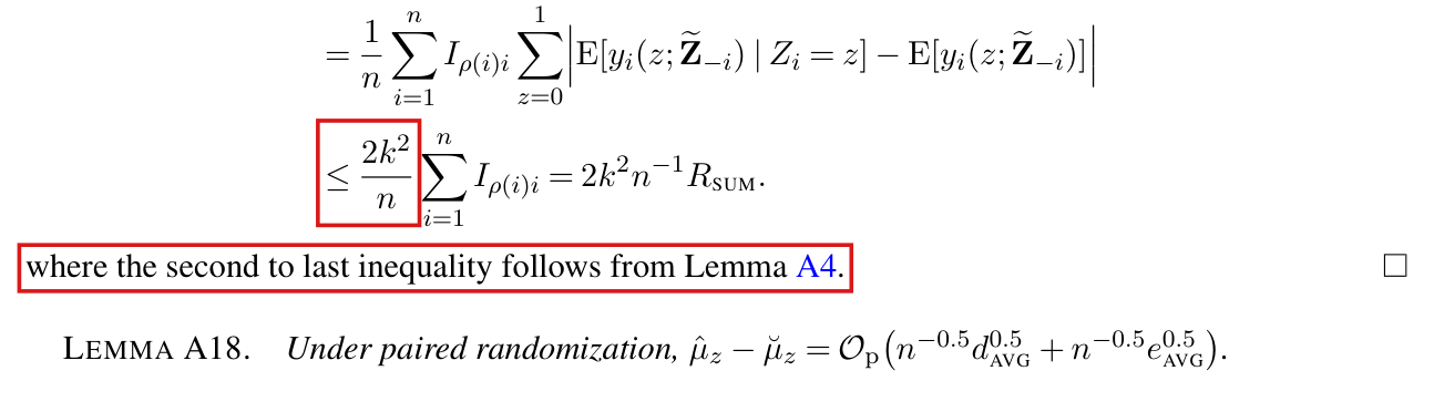
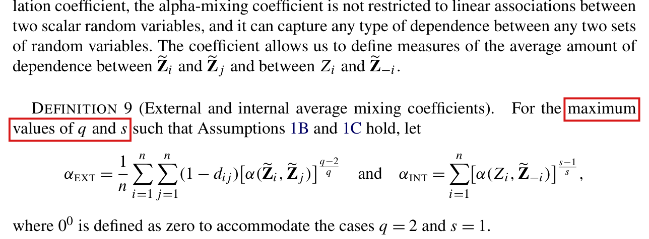
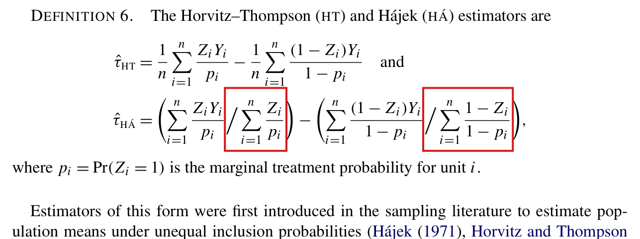
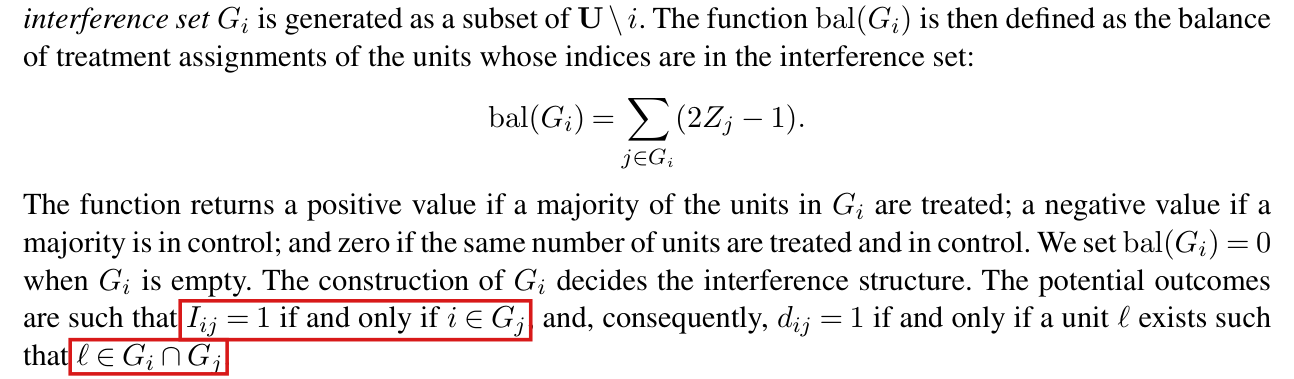
Standing assumptions: [Setting: Section 3.1, p. 676 (PDF p. 4)] Consider a sample of $n$ units indexed by the set $\mathbf{U} = \{1, 2, \ldots, n\}$. An experimenter intervenes on the world in ways that potentially affect the units. The intervention is described by a $n$-dimensional binary vector $\mathbf{z} = (z_1, z_2, \ldots, z_n) \in \{0, 1\}^n$. For short, we refer to $z_i$ as unit $i$'s treatment. Each unit has a function $y_i : \{0, 1\}^n \to \mathbb{R}$ denoting the observed outcome for the unit under a specific and potentially counterfactual intervention. In particular, $y_i(\mathbf{z})$ is the response of $i$ when the intervention is $\mathbf{z}$. We refer to the elements of the image of this function as potential outcomes. Let $\mathbf{z}_{-i} = (z_1, \ldots, z_{i-1}, z_{i+1}, \ldots, z_n)$ denote the $(n-1)$-dimensional vector constructed by deleting the $i$th element from $\mathbf{z}$. The potential outcome $y_i(\mathbf{z})$ can then be written as $y_i(z_i; \mathbf{z}_{-i})$. Throughout the paper, we assume that the potential outcomes are well-defined. The experimenter sets $\mathbf{z}$ according to a random vector $\mathbf{Z} = (Z_1, \ldots, Z_n)$. The probability distribution of $\mathbf{Z}$ is the design of the experiment. The design is the sole source of randomness we will consider. Let $Y_i$ denote the observed outcome of unit $i$: $Y_i = y_i(\mathbf{Z})$. As above, $\mathbf{Z}_{-i}$ denotes $\mathbf{Z}$ without its $i$th element, so $Y_i = y_i(Z_i; \mathbf{Z}_{-i})$. [No interference: Section 3.2, p. 676 (PDF p. 4)] It is conventional to assume that the potential outcomes are restricted so a unit's outcome is only affected by its own treatment. That is, for any two assignments $\mathbf{z}$ and $\mathbf{z}'$, if the treatment of a given unit is the same for both assignments, then the outcome for that unit is also the same. This no-interference assumption admits a definition of the treatment effect $\tau_i$ for unit $i$: $\tau_i = y_i(1; \mathbf{z}_{-i}) - y_i(0; \mathbf{z}_{-i})$, where $\mathbf{z}_{-i}$ is any element of $\{0, 1\}^{n-1}$. [Definitions 1 to 3: p. 677 (PDF p. 5)] DEFINITION 1. Under no interference, the average treatment effect (ATE) is the average unit-level treatment effect: $\tau_{\mathrm{ATE}} = \frac{1}{n}\sum_{i=1}^{n} \tau_i$. The assignment-conditional unit-level treatment effect is $\tau_i(\mathbf{z}_{-i}) = y_i(1; \mathbf{z}_{-i}) - y_i(0; \mathbf{z}_{-i})$. DEFINITION 2. An assignment-conditional average treatment effect is the average of the assignment-conditional unit-level treatment effects under a given assignment: $\tau_{\mathrm{ATE}}(\mathbf{z}) = \frac{1}{n}\sum_{i=1}^{n} \tau_i(\mathbf{z}_{-i})$. DEFINITION 3. The expected average treatment effect (EATE) is the expected assignment-conditional average treatment effect: $\tau_{\mathrm{EATE}} = \mathrm{E}[\tau_{\mathrm{ATE}}(\mathbf{Z})]$, where the expectation is taken over the distribution of $\mathbf{Z}$ given by the experimental design. [Definition 4: p. 678 (PDF p. 6)] DEFINITION 4. The average distributional shift effect (ADSE) is the average difference between the conditional expected outcomes for the two treatment conditions: $\tau_{\mathrm{ADSE}} = \frac{1}{n}\sum_{i=1}^{n}\left(\mathrm{E}[Y_i \mid Z_i = 1] - \mathrm{E}[Y_i \mid Z_i = 0]\right)$. [Interference indicator: Section 4, p. 680 (PDF p. 8)] We say that unit $i$ interferes with unit $j$ if changing $i$'s treatment changes $j$'s outcome under at least one treatment assignment. We also say that a unit interferes with itself even if its own treatment does not affect its outcome. The indicator $I_{ij}$ denotes such interference: $I_{ij} = \begin{cases} 1 & \text{if } y_j(\mathbf{z}) \ne y_j(\mathbf{z}') \text{ for some } \mathbf{z}, \mathbf{z}' \in \{0, 1\}^n \text{ such that } \mathbf{z}_{-i} = \mathbf{z}'_{-i}, \\ 1 & \text{if } i = j, \\ 0 & \text{otherwise.} \end{cases}$ [Definition 5 (Interference dependence): p. 681 (PDF p. 9)] $d_{\mathrm{AVG}} = \frac{1}{n}\sum_{i=1}^{n}\sum_{j=1}^{n} d_{ij}$ where $d_{ij} = \begin{cases} 1 & \text{if } I_{\ell i} I_{\ell j} = 1 \text{ for some } \ell \in \mathbf{U}, \\ 0 & \text{otherwise.} \end{cases}$ The sum $d_i = \sum_{j=1}^{n} d_{ij}$ gives the number of interference dependencies for unit $i$. [Interference counts: p. 681 (PDF p. 9)] $c_i = \sum_{j=1}^{n} I_{ij}$ and $C_p = \left[\frac{1}{n}\sum_{i=1}^{n} c_i^p\right]^{1/p}$. We write $C_\infty$ for the limit of $C_p$ as $p \to \infty$, which is the maximum $c_i$ over $\mathbf{U}$. [Asymptotic regime: Section 5, pp. 681–682 (PDF pp. 9–10)] We consider an arbitrary sequence of samples indexed by their sample size. The samples are not assumed to be drawn from some larger population or otherwise randomly generated. All quantities describing the samples, such as the potential outcomes and experimental designs, have their own sequences also indexed by $n$. But we leave the indexing implicit as no confusion arises. [Definition 6: p. 682 (PDF p. 10)] The Horvitz–Thompson (HT) and Hájek (HÁ) estimators are $\hat\tau_{\mathrm{HT}} = \frac{1}{n}\sum_{i=1}^{n}\frac{Z_i Y_i}{p_i} - \frac{1}{n}\sum_{i=1}^{n}\frac{(1 - Z_i)Y_i}{1 - p_i}$ and $\hat\tau_{\mathrm{H\acute{A}}} = \left(\sum_{i=1}^{n}\frac{Z_i Y_i}{p_i} \Big/ \sum_{i=1}^{n}\frac{Z_i}{p_i}\right) - \left(\sum_{i=1}^{n}\frac{(1 - Z_i)Y_i}{1 - p_i} \Big/ \sum_{i=1}^{n}\frac{1 - Z_i}{1 - p_i}\right)$, where $p_i = \Pr(Z_i = 1)$ is the marginal treatment probability for unit $i$. [Assumption 1: p. 682 (PDF p. 10)] We assume throughout the remainder of the paper that the experimental design and potential outcomes are sufficiently well behaved, as formalized in the following assumption. ASSUMPTION 1 (Regularity conditions). There exist constants $k < \infty$, $q \ge 2$ and $s \ge 1$ such that for all $i \in \mathbf{U}$ in the sequence of samples: A (Probabilistic assignment). $k^{-1} \le \Pr(Z_i = 1) \le 1 - k^{-1}$, B (Outcome moments). $\mathrm{E}[|Y_i|^q] \le k^q$, C (Potential outcome moments). $\mathrm{E}[|y_i(z; \mathbf{Z}_{-i})|^s] \le k^s$ for $z \in \{0, 1\}$. [Assumption 2: p. 683 (PDF p. 11)] ASSUMPTION 2 (Restricted interference). $d_{\mathrm{AVG}} = o(n)$. [Bernoulli design: p. 683 (PDF p. 11)] We call this a Bernoulli randomization design, and it satisfies $\Pr(\mathbf{Z} = \mathbf{z}) = \prod_{i=1}^{n} p_i^{z_i}(1 - p_i)^{1 - z_i}$ for some set of assignment probabilities $p_1, p_2, \ldots, p_n$ bounded away from zero and one. [Complete randomization: p. 684 (PDF p. 12)] $\Pr(\mathbf{Z} = \mathbf{z}) = \begin{cases} \binom{n}{m}^{-1} & \text{if } \sum_{i=1}^{n} z_i = m, \\ 0 & \text{otherwise,} \end{cases}$ where $m = \lfloor pn \rfloor$ for some fixed $p$ strictly between zero and one. We call the design complete randomization. [Paired randomization: p. 685 (PDF p. 13)] It is implicit that the sample size is even so that all units are paired. Let $\rho : \mathbf{U} \to \mathbf{U}$ describe a pairing so that $\rho(i) = j$ indicates that units $i$ and $j$ are paired. The pairing is symmetric, so the self-composition of $\rho$ is the identity function. The paired randomization design then satisfies $\Pr(\mathbf{Z} = \mathbf{z}) = \begin{cases} 2^{-n/2} & \text{if } z_i \ne z_{\rho(i)} \text{ for all } i \in \mathbf{U}, \\ 0 & \text{otherwise.} \end{cases}$ [Notation the paper uses without defining] The paper does not define $\mathcal{O}_p$, $o_p$, 'consistent' or 'root-$n$ consistent'. The proof of Lemma A5 (Supplement A, p. 4) uses $X_n - x_n = \mathcal{O}_p(a_n)$ in the sense that for every $\varepsilon > 0$ there are a constant $\kappa$ and an $N$ such that $\Pr(|X_n - x_n| \ge \kappa a_n) \le \varepsilon$ for all $n \ge N$. 'Consistent for' an estimand means that the difference between the estimator and the estimand (both sequences in $n$) converges in probability to zero; 'root-$n$ consistent' means that this difference is $\mathcal{O}_p(n^{-0.5})$. Supplement A is the separate file 'Supplement A: Proofs' (41 pp., DOI 10.1214/20-AOS1973SUPPA) and Supplement B is 'Supplement B: Simulation study' (21 pp., DOI 10.1214/20-AOS1973SUPPB); their page numbers are their own printed page numbers, which equal their PDF page numbers. In the main article the printed page number is the PDF page number plus 672.
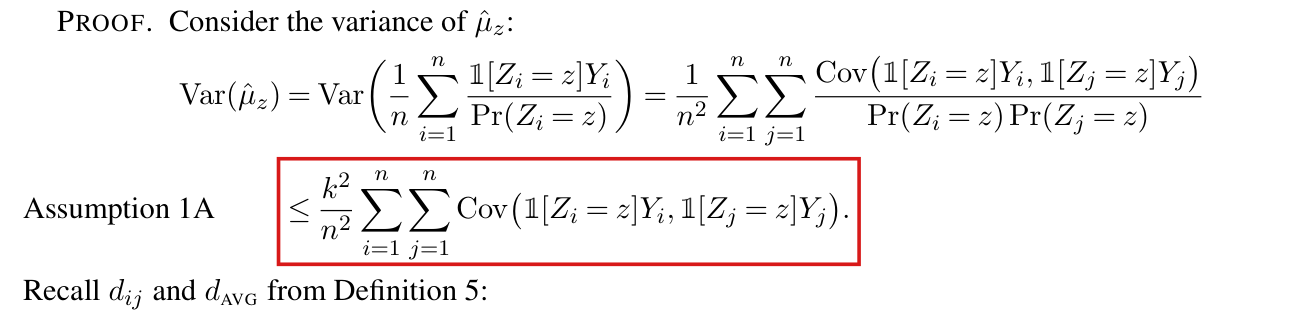
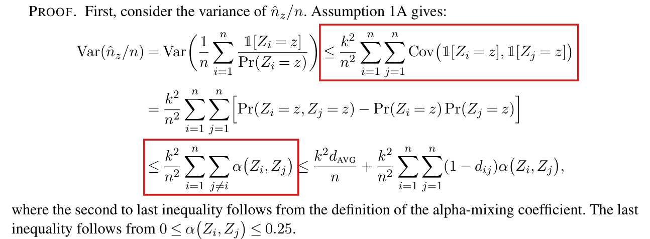
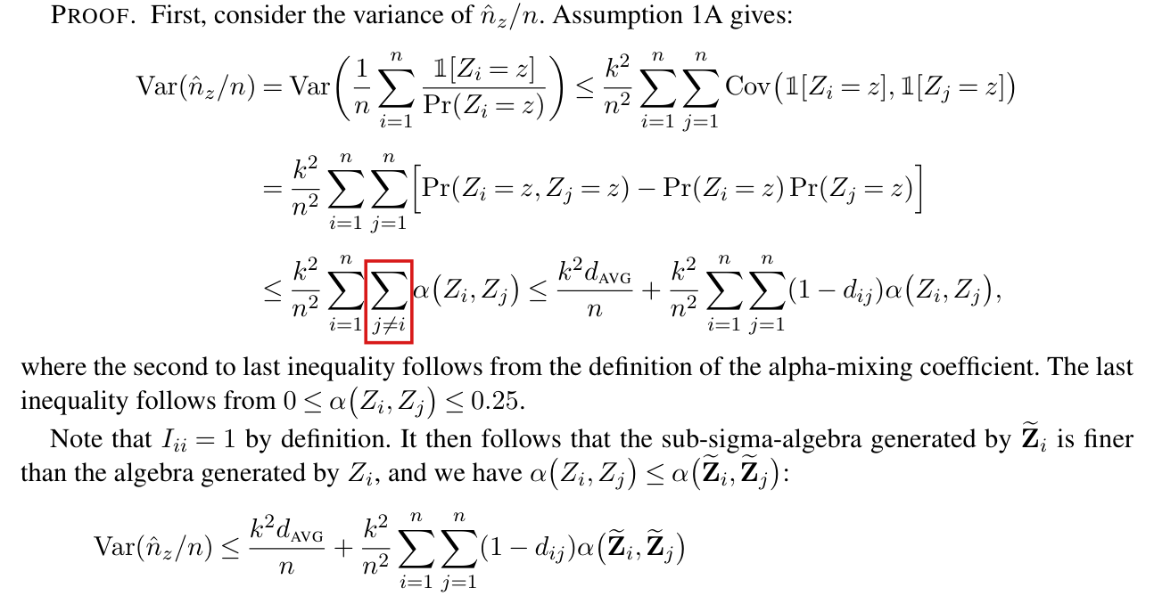
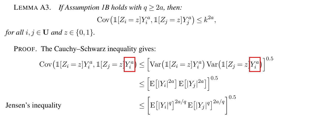
Effective claim (source TeX): [Printed steps] [Supplement A, p. 8, proof of Lemma A9] Consider the variance of $\hat\mu_z$: $\mathrm{Var}(\hat\mu_z) = \mathrm{Var}\left(\frac{1}{n}\sum_{i=1}^{n}\frac{\mathbb{1}[Z_i = z]Y_i}{\Pr(Z_i = z)}\right) = \frac{1}{n^2}\sum_{i=1}^{n}\sum_{j=1}^{n}\frac{\mathrm{Cov}\left(\mathbb{1}[Z_i = z]Y_i,\ \mathbb{1}[Z_j = z]Y_j\right)}{\Pr(Z_i = z)\Pr(Z_j = z)}$ [Assumption 1A] $\le \frac{k^2}{n^2}\sum_{i=1}^{n}\sum_{j=1}^{n}\mathrm{Cov}\left(\mathbb{1}[Z_i = z]Y_i,\ \mathbb{1}[Z_j = z]Y_j\right)$. [p. 22, proof of Lemma A22] Assumption 1A gives: $\mathrm{Var}(\hat\mu_z) = \mathrm{Var}\left(\frac{1}{n}\sum_{i=1}^{n}\frac{\mathbb{1}[Z_i = z]Y_i}{\Pr(Z_i = z)}\right) \le \frac{k^2}{n^2}\sum_{i=1}^{n}\sum_{j=1}^{n}\mathrm{Cov}\left(\mathbb{1}[Z_i = z]Y_i,\ \mathbb{1}[Z_j = z]Y_j\right)$. [p. 23, proof of Lemma A23] First, consider the variance of $\hat n_z/n$. Assumption 1A gives: $\mathrm{Var}(\hat n_z/n) = \mathrm{Var}\left(\frac{1}{n}\sum_{i=1}^{n}\frac{\mathbb{1}[Z_i = z]}{\Pr(Z_i = z)}\right) \le \frac{k^2}{n^2}\sum_{i=1}^{n}\sum_{j=1}^{n}\mathrm{Cov}\left(\mathbb{1}[Z_i = z],\ \mathbb{1}[Z_j = z]\right)$. [p. 25, proof of Lemma A25] Given Assumption 1A, for $z \in \{0, 1\}$: $\mathrm{Var}\left(\sum_{i=1}^{n}\frac{\mathbb{1}[Z_i = z]Y_i^2}{[\Pr(Z_i = z)]^2}\right) \le k^4\sum_{i=1}^{n}\sum_{j=1}^{n}\mathrm{Cov}\left(\mathbb{1}[Z_i = z]Y_i^2,\ \mathbb{1}[Z_j = z]Y_j^2\right)$. [What is refuted] Each printed inequality, in which unequal positive weights are replaced by their upper bound inside a sum of signed covariances. The conclusions of the four lemmas are not refuted. [Counterexamples, from the validator; in all three $n = 2$, $z = 1$, $k = 4$, and all potential outcomes have absolute value at most 1, so Assumption 1 holds for every $q \ge 2$ and $s \ge 1$] (i) Lemmas A9 and A22. $Z_1 \sim$ Bernoulli($\frac{1}{4}$) and $Z_2 \sim$ Bernoulli($\frac{3}{4}$), independent; $y_1(z_1, z_2) = z_2$ and $y_2(z_1, z_2) = -z_1$. With $B = Z_1 Z_2$: $\mathbb{1}[Z_1 = 1]Y_1 = B$, $\mathbb{1}[Z_2 = 1]Y_2 = -B$, $\Pr(B = 1) = \frac{3}{16}$, $\mathrm{Var}(B) = \frac{39}{256}$, and the four covariances are $\frac{39}{256}, -\frac{39}{256}, -\frac{39}{256}, \frac{39}{256}$, with sum 0. But $\hat\mu_1 = \frac{4}{3}B$ and $\mathrm{Var}(\hat\mu_1) = \frac{13}{48} > 0 = \frac{k^2}{n^2}\sum_{i,j}\mathrm{Cov}(\mathbb{1}[Z_i = 1]Y_i, \mathbb{1}[Z_j = 1]Y_j)$. (A Bernoulli design is one of the arbitrary designs of Lemma A22.) (ii) Lemma A23. The design $\Pr(\mathbf{Z} = (1, 0)) = \frac{1}{4}$, $\Pr(\mathbf{Z} = (0, 1)) = \frac{3}{4}$, with all potential outcomes equal to 1. Then $Z_1 + Z_2 = 1$ surely, so $\sum_{i,j}\mathrm{Cov}(\mathbb{1}[Z_i = 1], \mathbb{1}[Z_j = 1]) = 0$, while $\hat n_1/n$ equals 2 with probability $\frac{1}{4}$ and $\frac{2}{3}$ with probability $\frac{3}{4}$, so $\mathrm{Var}(\hat n_1/n) = \frac{1}{3} > 0$. (iii) Lemma A25. $Z_1 \sim$ Bernoulli($\frac{1}{4}$) and $Z_2 \sim$ Bernoulli($\frac{3}{4}$), independent; $y_1(z_1, z_2) = 1$ and $y_2(z_1, z_2) = 1 - z_1$. With $T_1 = \mathbb{1}[Z_1 = 1]Y_1^2 = Z_1$ and $T_2 = \mathbb{1}[Z_2 = 1]Y_2^2 = Z_2(1 - Z_1)$: $\sum_{i,j}\mathrm{Cov}(T_i, T_j) = \mathrm{Var}(T_1 + T_2) = \frac{39}{256}$, so the printed bound is $k^4 \cdot \frac{39}{256} = 39$; but $W = T_1/p_1^2 + T_2/p_2^2 = 16T_1 + \frac{16}{9}T_2$ takes the values $0, \frac{16}{9}, 16$ with probabilities $\frac{3}{16}, \frac{9}{16}, \frac{1}{4}$, so $\mathrm{E}[W] = 5$, $\mathrm{E}[W^2] = \frac{592}{9}$ and $\mathrm{Var}(W) = \frac{367}{9} > 39$.
: SAP.P009a.T3WholeStatement
Theorem: SAP.P009a.T3
Statement hash: 33cfd3b654477ceace203cc9605b4989c5f548efc8c946574af29ece1321ffb5
Statement definition: SAP.P009a.T3WholeStatement
Certificate. 20261104T180339Z
Declaration review: faithful; 2026-11-04T18:39:19Z; binding v2
Evidence scope: Certification checks formal proof objects. Statement fidelity is a model judgment. Author review is separate.
Proof dependencies: Independently extracted
Manifest annotation reconciliation: Effective use follows the source-bound dependency observation; original annotations are retained in the crosswalk.
AronowAudit.P009.sum_cube_succ: observed used
Source and evidence metadata · sap-2026-11-08-assured-release