P011-E001 Critical
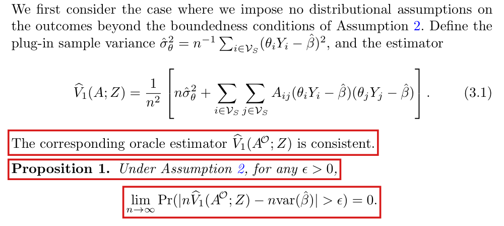
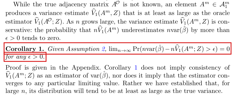
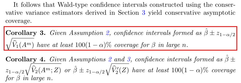
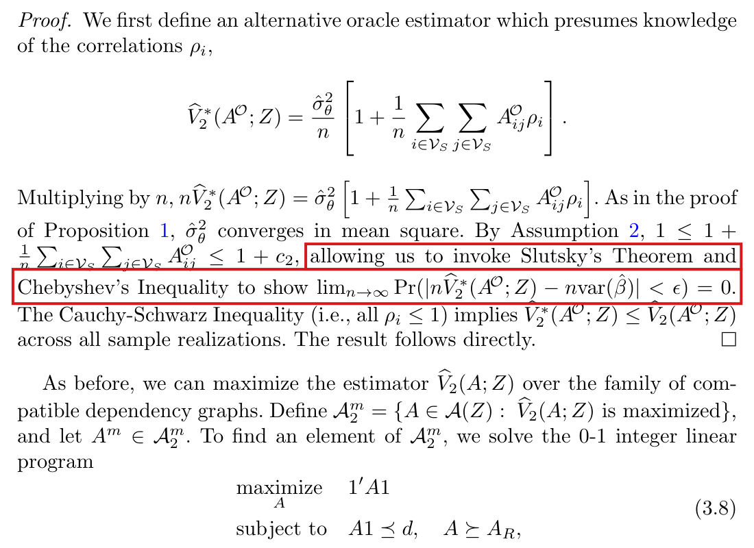
Under Assumption 2 the oracle estimator satisfies with , and the term on the right can be negative; Proposition 1, Corollaries 1 and 3 and the sentence after Assumption 3 therefore hold only under a further condition on the unit means, on the graph, or on the known edges and remaining degree capacity.
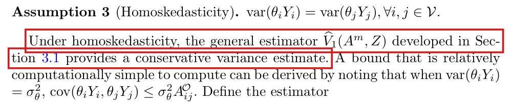
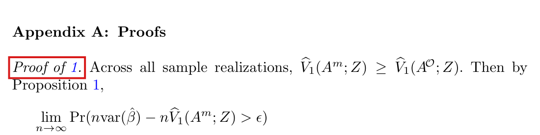
Section 3.1, p. 2242 (PDF p. 5): equation (3.1), the sentence after it and Proposition 1. Proof of Proposition 1, p. 2243 (PDF p. 6). Corollary 1, p. 2245 (PDF p. 8). First sentence after Assumption 3, p. 2246 (PDF p. 9). Corollary 3, p. 2248 (PDF p. 11). The abstract, p. 2238, states the same claims.
See also under Formal statements (Lean): P011-T1, P011-T2, P011-T3, P011-T4, P011-T5, P011-T6, P011-T7, P011-T8, P011-T9, P011-T10, P011-T16, P011-T29, P011-T31, P011-T32, P011-T33, P011-T41
As printed
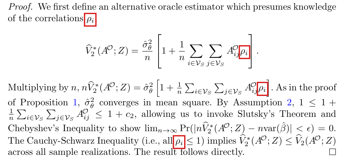
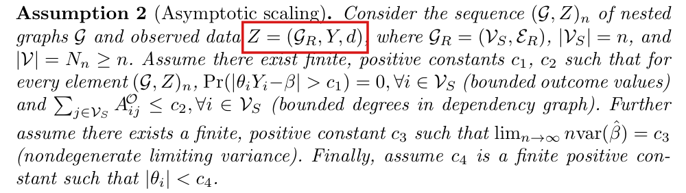
P. 2242: “The corresponding oracle estimator is consistent. Proposition 1. Under Assumption 2, for any , .”
P. 2243, in the proof: “Asymptotic unbiasedness follows directly from linearity of expectations and .”
P. 2245: “Corollary 1. Given Assumption 2, for any .”
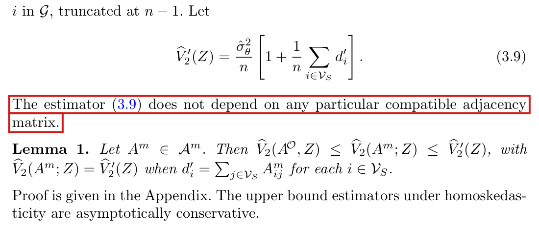
P. 2246: “Under homoskedasticity, the general estimator developed in Section 3.1 provides a conservative variance estimate.”
P. 2248: “Corollary 3. Given Assumption 2, confidence intervals formed as have at least coverage for in large .”
The problem
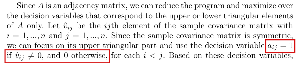
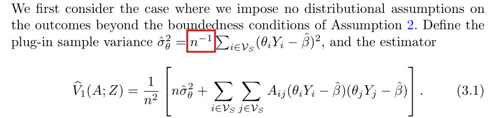
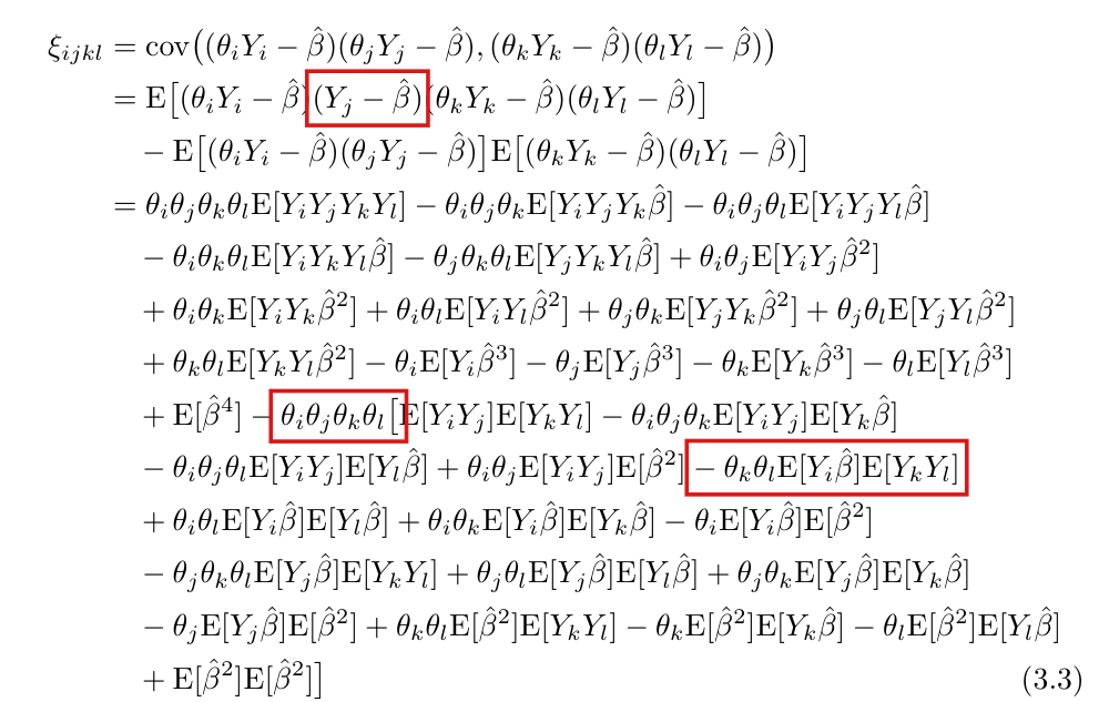
Definition 3 requires that the average of the unit means equal . It does not require that each unit mean equal . In the leading example of the paper, an OLS coefficient with , the unit means can differ. The estimator (3.1) centres every at the single number . Let and . Then , and the products need not average out. Under Assumption 2,
The step of the proof that asserts asymptotic unbiasedness omits the term on the right. The same omission affects , whose asymptotic approximation includes .
Note that the term on the right is deterministic. It need not tend to zero, and Proposition 1 fails. Since the matrix is positive semidefinite only when the graph is a disjoint union of cliques, the term can be negative. The oracle estimator then underestimates the variance. If the known edges and the degrees determine the graph, then , and the maximal compatible estimator underestimates the variance as well. Corollaries 1 and 3 fail in that case. Assumption 3 equalizes the variances of the and not their means. The examples below are homoskedastic, which shows that the sentence on p. 2246 fails too. The abstract states the consistency of the oracle estimator and conservative coverage without the condition.
The condition is necessary and sufficient for Proposition 1 under Assumption 2. It restricts the unit means, and a correctly specified OLS model does not imply it. No estimator is consistent, at the scale of times the variance, for every bounded configuration of unit means. Indeed, let and with independent fair signs . For each fixed infinite sequence of signs , I have . If the are themselves independent fair signs, then . An estimator that is consistent under every fixed infinite sequence tends to in the second model as well, where the target is . Proposition 1 holds exactly when the term displayed above tends to zero. Conservativeness of the maximized estimator requires less: an additional condition on the known edges, remaining degree capacity and relevant mean directions supplies further sufficient cases without changing the estimator. This condition does not imply consistency of the original oracle. Fixed positive semidefinite corrections or suitable regression residuals provide other repairs; the resulting maximal bounds are conservative and need not be consistent.
Evidence an exact counterexample
I use a derivation of the displayed identity and exact counterexamples to the printed statements. For the identity, let , and . Then
Since unless or , I have . Each variable is bounded by and depends only on the outcomes of and its neighbours. Two such variables are independent when their vertices are at graph distance greater than three. Counting the pairs that may be dependent, I obtain . Further, , and the last two terms of the display are at most in absolute value. Chebyshev’s inequality then implies that the identity holds.
The first example consists of independent blocks of three units , , on a path. Let and be independent fair signs, let , and set
Since the outcomes of and are independent, the path is a dependency graph. Every variance equals 1, the unit means are , and . All edges are known and the degrees are , which implies that is the only compatible matrix. Assumptions 1, 2 and 3 hold. By an exact enumeration, I have and , and tends to in probability. For every , the probability in Corollary 1 tends to one. The coverage of the nominal 95% interval tends to . This example is a correctly specified regression with covariate , intercept 0 and slope 1, in which is the fitted intercept. With the unit means doubled, tends to , and the estimate is negative with probability tending to one.
The second example consists of independent blocks of four units on a cycle. Each edge carries an independent fair sign, is plus the two signs on the edges at , with , and . The covariance matrix of a block is , every edge is known and every degree is 2. Then and tends to . For the limit is , the exact mean is , and the coverage of the nominal 95% interval tends to about .
| Example | Limit of | Coverage | |
|---|---|---|---|
| Paths of three, unit means | |||
| Paths of three, unit means | – | ||
| Cycles of four, unit means |
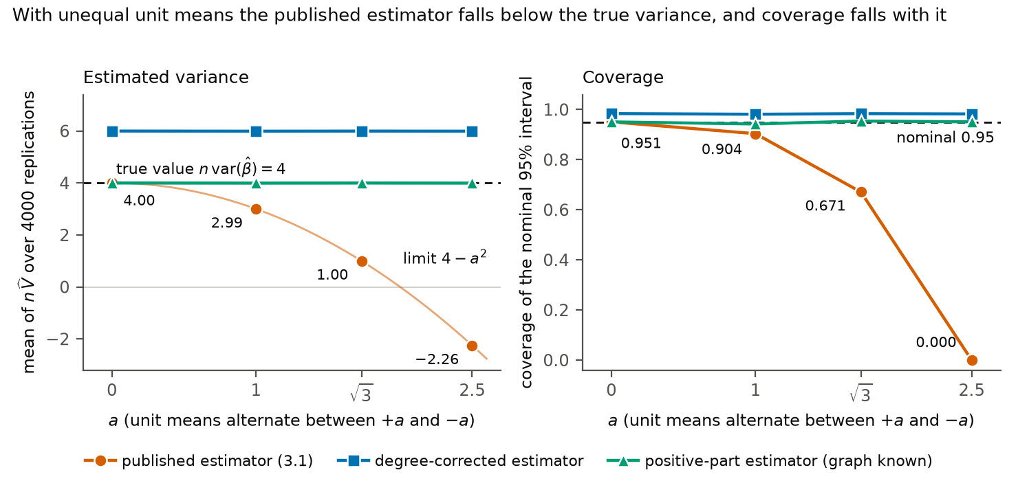
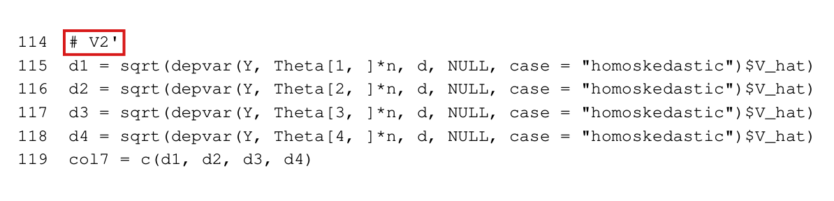
Simulations of the second example, which I call example A, agree with these limits. The figure shows them for four values of . The next table adds example B, a difference in means on the same cycles. The units of a cycle alternate between treatment and control, is plus the two edge signs plus an independent unit sign, and . In this example, , and the unit means are . The estimators , and are defined in the corrected statements below. Residual centering replaces by times the deviation of from the mean of its arm.
| Estimator | A: | A: coverage | B: | B: coverage |
|---|---|---|---|---|
| , as published | 1.00 | 0.671 | 0.00 | 0.222 |
| 5.99 | 0.984 | 16.00 | 1.000 | |
| 15.00 | 1.000 | 47.99 | 1.000 | |
| 4.00 | 0.954 | 9.00 | 0.997 | |
| Residual centering | – | – | 4.01 | 0.950 |
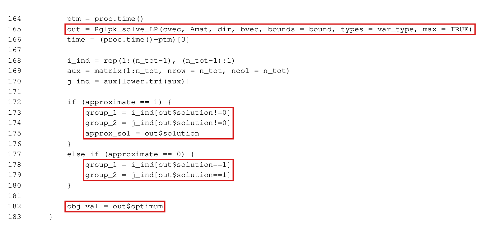
The last table concerns the unknown graph. The maximization over compatible graphs is solved by integer programming, with , degree bounds and the two examples of the previous table. With no known edge the published estimator is conservative. It fails when the known edges fix most of the graph.
| Example | Known edges | Coverage | Coverage | ||
|---|---|---|---|---|---|
| A | none | 14.90 | 1.000 | 14.90 | 1.000 |
| A | 27 of the 30 cycles | 2.20 | 0.826 | 7.16 | 0.994 |
| A | 108 of the 120 edges | 2.25 | 0.835 | 7.21 | 0.994 |
| A | all | 0.91 | 0.587 | 5.87 | 0.977 |
| B | none | 47.76 | 1.000 | 47.77 | 1.000 |
| B | 27 of the 30 cycles | 4.22 | 0.842 | 20.14 | 1.000 |
| B | 108 of the 120 edges | 4.32 | 0.885 | 20.24 | 1.000 |
| B | all | 0.333 | 15.77 | 1.000 |
The simulations illustrate the limits and are not part of the argument. The term can also be zero or positive, and unequal unit means do not always make the published estimator anticonservative.
What survives
The following are unaffected.
- The definitions, and the inequality in every sample.
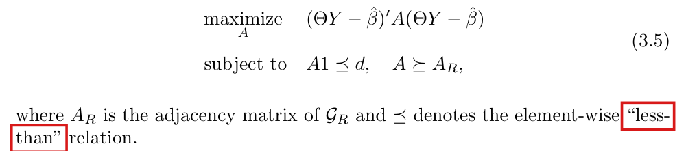
- The programs (3.5), (3.6) and (3.8) as optimization problems.
- The bound of order on the variance of the estimator in the proof of Proposition 1, after the corrections to display (3.3) in
P011-E003. - The central limit theorem of Lemma 2.
- Lemma 3 and Proposition 3, which are conditional on a property of the variance estimator.
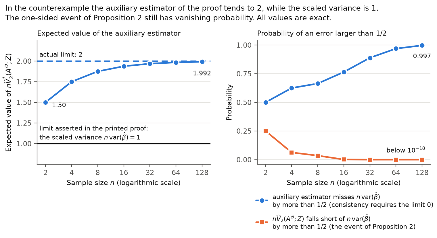
The conclusions of Proposition 2, Lemma 1 and Corollaries 2 and 4 for and hold with unequal unit means, by a direct argument, although the printed proof of Proposition 2 does not (see P011-E004).
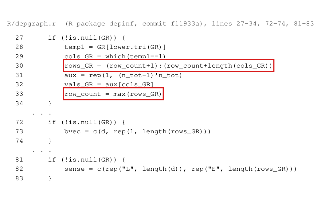
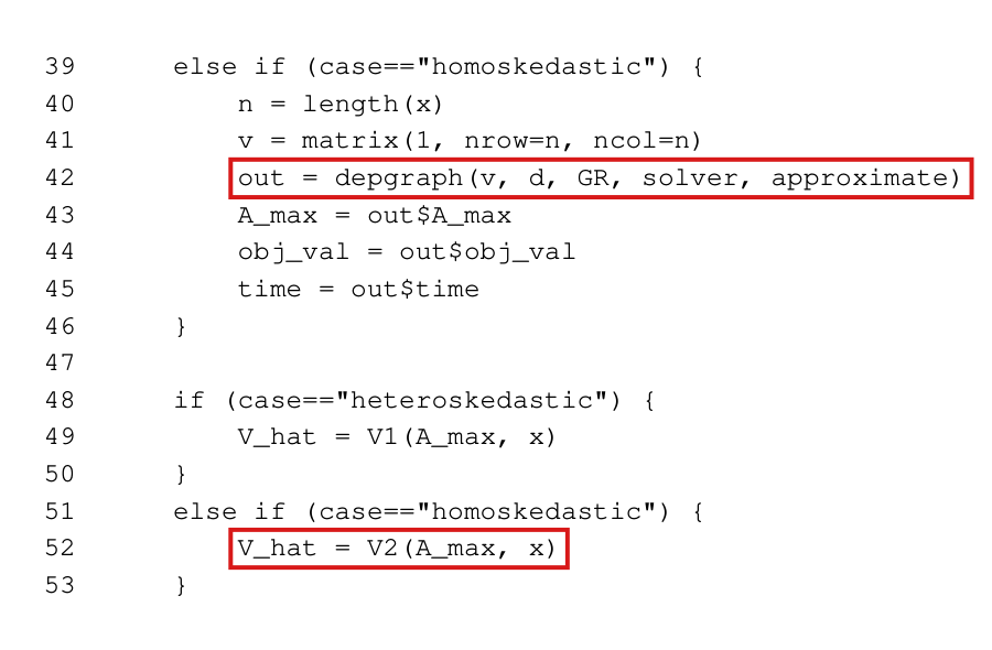
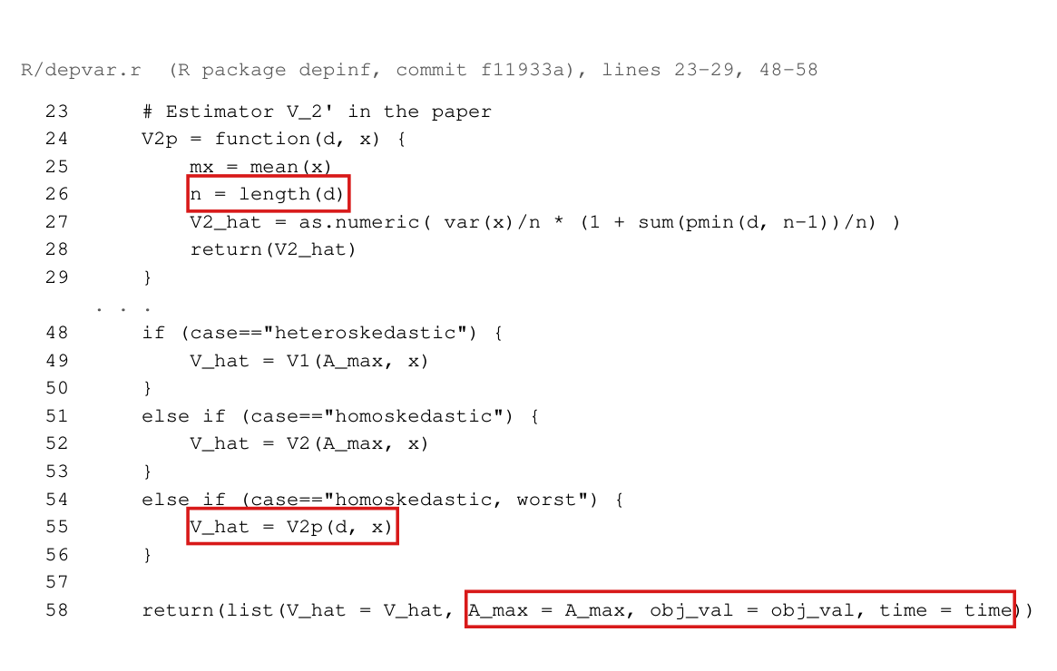
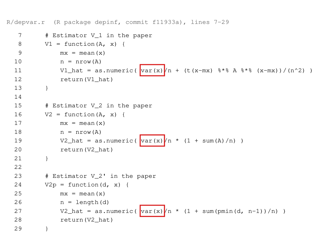
The general guarantees need qualification when unit means differ and edges are known: Proposition 1, Corollaries 1 and 3, the sentence on p. 2246, and the corresponding claims of the abstract, the introduction and the discussion. The corrected conservativeness condition below retains the original maximized estimator in additional graph and mean configurations, including sparse known edges and known graphs close to disjoint cliques. It does not remove the need for an additional condition, and homoskedasticity alone does not supply one. The heteroskedastic branch of the package computes the same estimator, and its vignette applies it to OLS coefficients with known recruitment edges (see P011-N006). The article reports no simulation or application results, so no empirical number changes. I have not established that any interval in the vignette undercovers.
Corrected
Throughout, , , , and .
Proposition 1. Under Assumption 2, for any ,
Hence the conclusion of Proposition 1 as printed holds if and only if . It holds in particular if for every . In the proof, the sentence on asymptotic unbiasedness becomes .
Corollary 1: a broader sufficient condition. Retain Assumptions 1–2 and the original point estimator. Let be the known-edge adjacency matrix. Choose fixed valid integer caps
and define
The original maximization may retain larger supplied caps. Let be fixed with , and write the variance inputs as
where is deterministic. Here is the centering error for these inputs; for the published inputs , it is the original . All the other input conditions then follow from Assumption 2. Define
If condition (C) holds,
then, for every ,
For and this is the original maximized estimator. Condition (C) concerns only the relevant mean directions: if and , it suffices that
The negative eigenvalues of the full matrix need not vanish.
For , each of the following ensures (C). The first two use published centering, for which the mean deviations are uniformly bounded.
- There are known edges. This includes degree-only constraints, with no known edges.
- Deleting known edges leaves vertex-disjoint clique components. In particular, it suffices that only known edges belong to components that are not cliques. The retained clique edges may number and their caps need not be saturated. Exact disjoint cliques are a special case; overlapping cliques alone do not suffice.
- For every vertex, . Then
- The mean deviations lie in a specified space on which is positive semidefinite, or its smallest restricted eigenvalue tends to zero from below, as in the spectral condition above. Common transformed means, , give .
There is also the direct sufficient condition , from the corrected Proposition 1. A true graph consisting of disjoint cliques satisfies this condition for every mean vector. Neither this condition nor (C) requires the mean term to tend to zero, so neither establishes the published oracle’s consistency.
Two fixed corrections after maximization. For any mean vector satisfying the input conditions, (C) holds with
the negative spectral part of with its signs reversed, since . Alternatively, let be a fixed set of known edges whose deletion leaves vertex-disjoint cliques, and take its Laplacian . The added term is
There is no requirement that : if is the remaining adjacency matrix,
Both choices have bounded operator norm under the stated caps. Each is added after maximization, so it preserves the maximizing graph; either may widen the variance bound.
The sufficient condition follows from a compatible-graph construction and a variance calculation. Proper-color the known graph, sort the inputs within each color and remaining-capacity class, and join consecutive groups of vertices into cliques. The new edges respect all caps and do not duplicate known edges. The loss relative to is at most a constant depending on times , which gives
Put , and . If has degrees , then
Bounded-degree dependence gives and . The deterministic mean cross term is after division by , and the input remainder changes the quadratic form by on that scale. The possibly dense correction needs no local concentration argument: . Hence
which proves conservativeness under (C). The first two graph routes follow by bounding the adverse mean cross products by a constant times the number of exceptional known edges. The covariance and mean terms are separated in the same manner as in Yap’s Theorem 2; the graph construction and probability argument above are needed for this estimator.
Corollary 3. Given Assumptions 1–2 and the input conditions and condition (C) above, the intervals
have at least coverage for in large . The interval is taken to be empty when its variance estimate is negative; this event has probability tending to zero. The conclusion follows from Lemma 2 and the conservativeness bound, since tends to a positive constant. It does not require consistency of the maximum or of the original oracle. The same coverage conclusion holds for the original maximized estimator under the direct mean-term condition stated above.
Section 3.2, sentence after Assumption 3. “Under condition (C) with published centering and , the general estimator developed in Section 3.1 provides a conservative variance estimate.” The direct mean-term condition above is another sufficient qualification. Assumption 3 alone does not imply either one.
Estimators that are conservative for any unit means. For a compatible with degrees , define
where the summand of the first sum is zero when . Let maximize over . Given Assumption 2, for any unit means and any ,
for equal to , , , or the smaller of the last two. When the graph is known, the same holds for , where is obtained from by setting its negative eigenvalues to zero. These estimators are nonnegative, and by Proposition 3 their Wald intervals have at least coverage in large .
These statements hold for the following reason. Let be the covariance matrix of , and let be a deterministic symmetric matrix whose operator norm is bounded in . The same derivation gives
Both terms in the bracket are nonnegative when and are positive semidefinite. For , the matrix is the sum of , whose quadratic form is , and of the nonnegative diagonal matrix , where the ratio is zero when . The matrix is then a nonnegative diagonal matrix. For , since , I have in every sample, and for the matrix is the Laplacian of the graph, which is positive semidefinite. The maximum over is at least the oracle value in every sample, as in the proof of Corollary 1. The display must not be applied to a matrix that is chosen from the data. The no-known-edge case also follows directly from : if no edge is known and the bounds are at most , then in every sample, with . If the bounds are not bounded in , the same argument applies after each bound is replaced by the smaller of and the least integer above , which can only lower the maximum.
The estimator is affine in . Program (3.6) therefore applies with the weights , with interpreted as zero when , and , where is the optimal value. These estimators are conservative and in general not consistent. In the cycle example with and true value 4, the limits of , and are 6, 15 and 4.
Regression residuals. Retain the original point estimator. For nonrandom regressors , fit by -weighted least squares and use
only in the variance estimator. Let have rows and suppose ; a fixed number of regressors suffices. The conditions are met if , or, more generally, if
To see the prediction rate, let be the orthogonal projection onto and . The transformed fitted values are , including when coefficients are not unique or some weights are zero. Since ,
Thus with , , and . These bounds also imply and (C). Under exact specification . No separate coefficient-convergence rate or uniformly bounded-regressor assumption is required.
More generally, any predictions satisfying
can replace the weighted least-squares fit. In all these regression cases, the uncorrected true-graph residual oracle is consistent:
Indeed, and , so replacing by changes the scaled quadratic form by . The maximum over compatible graphs is conservative and need not be consistent. Adding can likewise introduce further conservativeness. Correct specification alone does not justify arbitrary unweighted fitting under the paper’s assumptions.
Abstract. “The oracle variance estimator has an asymptotic mean term. It is consistent, at the scale of times the variance, if and only if that term vanishes, and it can be anticonservative otherwise. The maximized estimator has asymptotically conservative coverage under the additional sufficient conditions stated above; fixed positive semidefinite corrections and suitable regression residuals provide further repairs.” The coverage guarantees of Corollary 4 are unaffected.












My comment and the history of this entry