LLM-generated corrections to the published research of P. M. Aronow

Journal article P011

Corrections to: Confidence Intervals for Linear Unbiased Estimators under Constrained Dependence

P. M. Aronow, Forrest W. Crawford, and Jose R. Zubizarreta (2018). Confidence Intervals for Linear Unbiased Estimators under Constrained Dependence. Electronic Journal of Statistics 12(2):2238–2252.

DOI
10.1214/18-ejs1448
arXiv
1602.00359
Audited edition
Electronic Journal of Statistics, 2018, 12(2):2238–2252; 15 pages in the audited file
SHA-256 of the audited file
cfc473501a3f3ed640d34f1b25eac188f9cfe85c6f916c10894dd0e97de97266
Permanent address
https://pmaronow.github.io/llm-audit/works/P011/

Summary

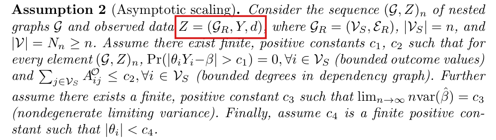
The paper constructs confidence intervals for linear unbiased estimators, such as OLS coefficients, when outcomes are dependent and their dependency graph is only partly known. It maximizes a variance estimator over the graphs compatible with the known edges and degrees, and proposes Wald intervals from that bound. 17 entries are classified as errors (1 Critical, 2 Moderate, 14 Minor), and 1 is a clarity note. The raw-outcome oracle need not be consistent when transformed unit means differ (P011-E001). Further conditions on means, the known graph or remaining degree capacity can justify conservativeness of the maximized estimator; the finding also gives fixed corrections and conditional residual alternatives.

What was and was not checked

I list below the checks that found no error.

  • Definitions 1 and 2: the induced subgraph of the observed vertices is a dependency graph.
  • The matrix AOA^{\mathcal O} is compatible with ZZ, and V^(Am;Z)≥V^(AO;Z)\widehat V(A^m;Z)\ge\widehat V(A^{\mathcal O};Z) in every sample.
  • The representation of an OLS coefficient as n−1∑iΘjiYin^{-1}\sum_i\Theta_{ji}Y_i and the formula for var⁡(β^)\operatorname{var}(\hat\beta) on p. 2241.
  • In the proof of Proposition 1: display (3.2), the covariance terms of display (3.4) after correcting the dropped weights in (3.3) (P011-E003), the count of the potentially nonzero leading covariance terms, and the resulting bound of order 1/n1/n on the variance of the estimator.
  • Program (3.6) as a reformulation of (3.5), program (3.8) as its unit-weight case, and the linear relaxation as an upper bound.
  • The statements of Proposition 2, Lemma 1 and Corollaries 2 and 4, by a direct argument that differs from the printed proof of Proposition 2; and the proof of Lemma 1.
  • Lemma 2, by a check that the hypotheses of the cited bound hold under Assumption 2; Lemma 3 and Proposition 3, which are conditional on a property of the variance estimator; and display (A.1), given Proposition 1.
  • In the package: the constraints built by depgraph agree with (3.6) on the tested inputs, and the regression coefficients, the classical and HC1 standard errors, and the linear-relaxation rows of the table of the vignette were reproduced with the GLPK solver.

I read the Gurobi and CPLEX branches of the package but did not run them because the solvers were unavailable. The columns of the table of the vignette that come from exact integer programs on the 522 observations were not recomputed. The paper’s cited sources were consulted only for the points of P011-N002. The article contains no table, figure or numerical result, so that there was nothing numerical in the article to recompute. The vignette refers to an application in “Section 5 of the paper”; Section 5 of the published article is the Discussion and contains no such application. An absence of corrections for a passage is not a finding that the passage is correct.

Further derivations in P011-E001 distinguish raw-outcome oracle consistency from conservativeness of the maximum over compatible graphs. They give sufficient graph, capacity and mean-space conditions, fixed positive semidefinite corrections, and a θi2\theta_i^2-weighted residual route with transformed design rank o(n)o(n) and exact or vanishing weighted mean-square specification error. The ordinary least-squares residual theorem in P011-N006 has stronger sufficient assumptions: fixed dimension, bounded outcomes and regressors, and a normalized Gram matrix with smallest eigenvalue bounded away from zero. Neither residual route changes the point estimator, and neither establishes consistency of the maximum. These conditional results do not establish that their application conditions hold for the vignette’s data.

Headline claims and related corrections

  1. With a known dependency graph, the oracle variance estimator V^1(AO;Z)\widehat V_1(A^{\mathcal O};Z) of (3.1) is consistent for var(β^)\mathrm{var}(\hat\beta) at the nn-scaled level under the boundedness and bounded-degree conditions of Assumption 2.

    Proposition 1; equation (3.1)

    See P011-E001, P011-E003.

  2. Under Assumption 2 (bounded outcomes, bounded dependency-graph degrees, positive limiting nn-scaled variance), (β^−β)/var(β^)(\hat\beta-\beta)/\sqrt{\mathrm{var}(\hat\beta)} converges in distribution to N(0,1)N(0,1).

    Lemma 2 (cited to Theorem 2.7 of Chen and Shao 2004)

  3. When the graph is unknown but degree bounds and some edges are known, maximizing over compatible adjacency matrices gives a sharp upper bound for the oracle estimated variance, and the maximization can be written as a 00–11 integer linear program.

    Definitions 4-6; programs (3.5), (3.6) and (3.8)

    See P011-E002, P011-E007, P011-E001.

  4. The maximal compatible estimator V^1(Am;Z)\widehat V_1(A^m;Z) is asymptotically conservative: Pr⁡(n var(β^)−nV^1(Am)>ϵ)→0\Pr(n\,\mathrm{var}(\hat\beta)-n\widehat V_1(A^m)>\epsilon)\to0.

    Corollary 1 (proof (A.1) in Appendix A)

    See P011-E001, P011-N007.

  5. Under homoskedasticity of the transformed outcomes θiYi\theta_iY_i (Assumption 3), the estimators V^2(AO)\widehat V_2(A^{\mathcal O}), V^2(Am)\widehat V_2(A^m) and the closed form V^2′(Z)\widehat V_2'(Z) of (3.9) are asymptotically conservative, with V^2(AO)≤V^2(Am)≤V^2′\widehat V_2(A^{\mathcal O})\le\widehat V_2(A^m)\le\widehat V_2'.

    Proposition 2; Lemma 1; Corollary 2 (and Corollary 4); equations (3.7)-(3.9)

    See P011-E004, P011-E005, P011-E006, P011-E001, P011-E012, P011-E013, P011-E015, P011-N001.

  6. Wald intervals β^±z1−α/2V^\hat\beta\pm z_{1-\alpha/2}\sqrt{\widehat V} built from the conservative variance estimators have asymptotic coverage of at least the nominal level.

    Lemma 3; Proposition 3; Corollaries 3 and 4

    See P011-E001.

  7. The framework applies to linear estimators that are unbiased when outcomes are neither independent nor identically distributed, including OLS coefficients, Horvitz-Thompson-type estimators and the difference in means.

    Definition 3 and the OLS example of Section 2; Propositions 1-3

    See P011-E001, P011-N006.

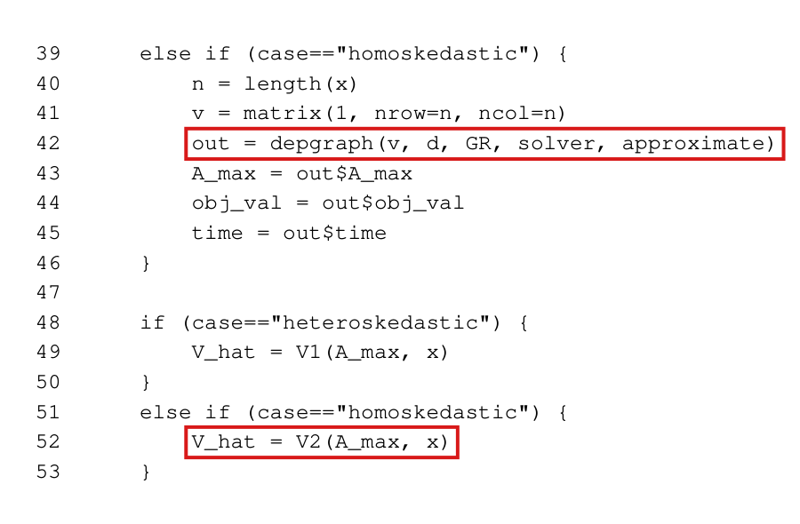
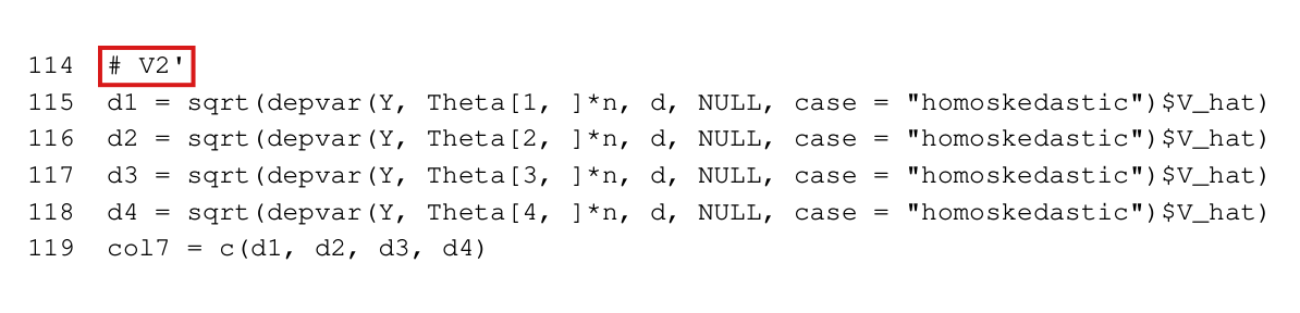
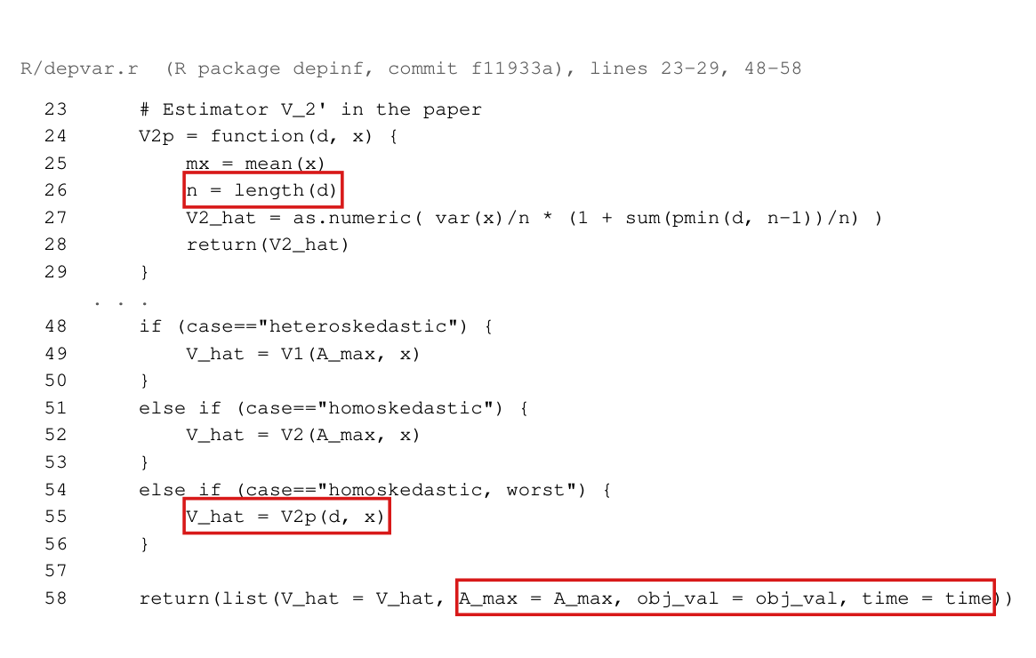
  8. The R package depinf implements the method: depgraph solves (3.5) and (3.8) exactly or by LP relaxation, and depvar computes (3.1) and (3.7).

    Appendix B (PDF p. 13, printed p. 2250); depinf: R/depgraph.r and R/depvar.r

    See P011-E011, P011-E012, P011-E013, P011-E014, P011-E015.

Corrections

Critical (1)

A headline conclusion is false or unsupported in the setting the paper targets, and no routine repair restores it.

Under Assumption 2 the oracle estimator satisfies nV^1(AO;Z)−nvar⁡(β^)=n−1δT(I+AO)δ+op(1)n\widehat V_1(A^{\mathcal O};Z)-n\operatorname{var}(\hat\beta)=n^{-1}\delta^{\mathsf T}(I+A^{\mathcal O})\delta+o_p(1) with δi=E[θiYi]−β\delta_i=\mathbb{E}[\theta_iY_i]-\beta, and the term on the right can be negative; Proposition 1, Corollaries 1 and 3 and the sentence after Assumption 3 therefore hold only under a further condition on the unit means, on the graph, or on the known edges and remaining degree capacity.

Section 3.1, p. 2242 (PDF p. 5): equation (3.1), the sentence after it and Proposition 1. Proof of Proposition 1, p. 2243 (PDF p. 6). Corollary 1, p. 2245 (PDF p. 8). First sentence after Assumption 3, p. 2246 (PDF p. 9). Corollary 3, p. 2248 (PDF p. 11). The abstract, p. 2238, states the same claims.

See also under Formal statements (Lean): P011-T1, P011-T2, P011-T3, P011-T4, P011-T5, P011-T6, P011-T7, P011-T8, P011-T9, P011-T10, P011-T16, P011-T29, P011-T31, P011-T32, P011-T33, P011-T41

My comment on this entry

As printed

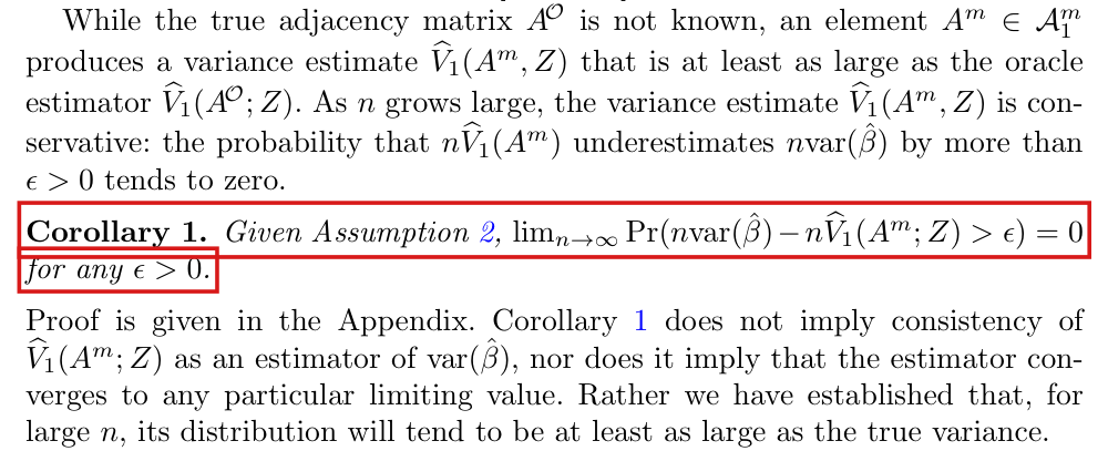
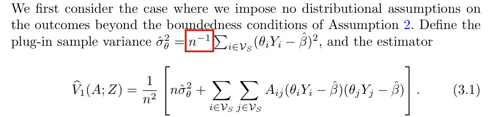
P. 2242: “The corresponding oracle estimator V^1(AO;Z)\widehat V_1(A^{\mathcal O};Z) is consistent. Proposition 1. Under Assumption 2, for any ϵ>0\epsilon>0, lim⁡n→∞Pr⁡(∣nV^1(AO;Z)−nvar⁡(β^)∣>ϵ)=0\lim_{n\to\infty}\Pr(|n\widehat V_1(A^{\mathcal O};Z)-n\operatorname{var}(\hat\beta)|>\epsilon)=0.”

P. 2243, in the proof: “Asymptotic unbiasedness follows directly from linearity of expectations and var⁡(β^)=O(n−1)\operatorname{var}(\hat\beta)=O(n^{-1}).”

P. 2245: “Corollary 1. Given Assumption 2, lim⁡n→∞Pr⁡(nvar⁡(β^)−nV^1(Am;Z)>ϵ)=0\lim_{n\to\infty}\Pr(n\operatorname{var}(\hat\beta)-n\widehat V_1(A^m;Z)>\epsilon)=0 for any ϵ>0\epsilon>0.”

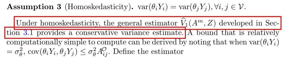
P. 2246: “Under homoskedasticity, the general estimator V^1(Am,Z)\widehat V_1(A^m,Z) developed in Section 3.1 provides a conservative variance estimate.”

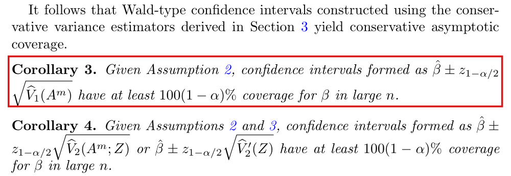
P. 2248: “Corollary 3. Given Assumption 2, confidence intervals formed as β^±z1−α/2V^1(Am)\hat\beta\pm z_{1-\alpha/2}\sqrt{\widehat V_1(A^m)} have at least 100(1−α)%100(1-\alpha)\% coverage for β\beta in large nn.”

The problem

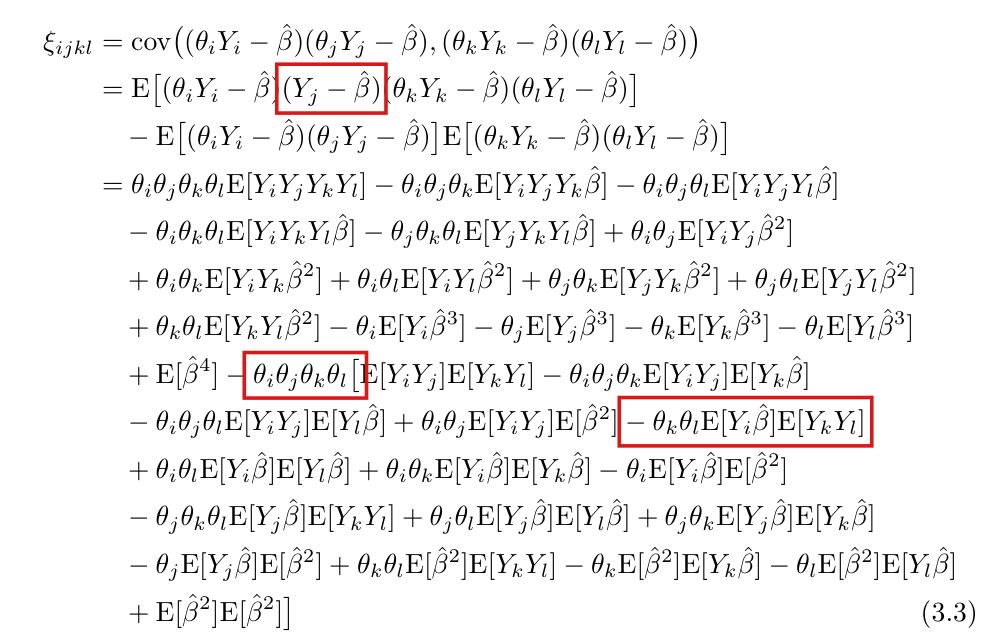
Definition 3 requires that the average of the unit means E[θiYi]\mathbb{E}[\theta_iY_i] equal β\beta. It does not require that each unit mean equal β\beta. In the leading example of the paper, an OLS coefficient with E[Yi]=xiTβ\mathbb{E}[Y_i]=x_i^{\mathsf T}\beta, the unit means can differ. The estimator (3.1) centres every θiYi\theta_iY_i at the single number β^\hat\beta. Let Xi=θiYiX_i=\theta_iY_i and δi=E[Xi]−β\delta_i=\mathbb{E}[X_i]-\beta. Then E[(Xi−β)(Xj−β)]=cov⁡(Xi,Xj)+δiδj\mathbb{E}[(X_i-\beta)(X_j-\beta)]=\operatorname{cov}(X_i,X_j)+\delta_i\delta_j, and the products δiδj\delta_i\delta_j need not average out. Under Assumption 2,

nV^1(AO;Z)−nvar⁡(β^)=1n δT(I+AO)δ+op(1).n\widehat V_1(A^{\mathcal O};Z)-n\operatorname{var}(\hat\beta)=\frac1n\,\delta^{\mathsf T}(I+A^{\mathcal O})\delta+o_p(1).

The step of the proof that asserts asymptotic unbiasedness omits the term on the right. The same omission affects σ^θ2\hat\sigma_\theta^2, whose asymptotic approximation includes n−1∑iδi2n^{-1}\sum_i\delta_i^2.

Note that the term on the right is deterministic. It need not tend to zero, and Proposition 1 fails. Since the matrix I+AOI+A^{\mathcal O} is positive semidefinite only when the graph GS\mathcal G_S is a disjoint union of cliques, the term can be negative. The oracle estimator then underestimates the variance. If the known edges and the degrees determine the graph, then Am=AOA^m=A^{\mathcal O}, and the maximal compatible estimator underestimates the variance as well. Corollaries 1 and 3 fail in that case. Assumption 3 equalizes the variances of the θiYi\theta_iY_i and not their means. The examples below are homoskedastic, which shows that the sentence on p. 2246 fails too. The abstract states the consistency of the oracle estimator and conservative coverage without the condition.

The condition n−1δT(I+AO)δ→0n^{-1}\delta^{\mathsf T}(I+A^{\mathcal O})\delta\to0 is necessary and sufficient for Proposition 1 under Assumption 2. It restricts the unit means, and a correctly specified OLS model does not imply it. No estimator is consistent, at the scale of nn times the variance, for every bounded configuration of unit means. Indeed, let a,b>0a,b>0 and Xi=asi+bϵiX_i=as_i+b\epsilon_i with independent fair signs ϵi\epsilon_i. For each fixed infinite sequence of signs sis_i, I have nvar⁡(β^)=b2n\operatorname{var}(\hat\beta)=b^2. If the sis_i are themselves independent fair signs, then nvar⁡(β^)=a2+b2n\operatorname{var}(\hat\beta)=a^2+b^2. An estimator that is consistent under every fixed infinite sequence tends to b2b^2 in the second model as well, where the target is a2+b2a^2+b^2. Proposition 1 holds exactly when the term displayed above tends to zero. Conservativeness of the maximized estimator requires less: an additional condition on the known edges, remaining degree capacity and relevant mean directions supplies further sufficient cases without changing the estimator. This condition does not imply consistency of the original oracle. Fixed positive semidefinite corrections or suitable regression residuals provide other repairs; the resulting maximal bounds are conservative and need not be consistent.

Evidence an exact counterexample

I use a derivation of the displayed identity and exact counterexamples to the printed statements. For the identity, let Wi=Xi−βW_i=X_i-\beta, D=β^−βD=\hat\beta-\beta and B=I+AOB=I+A^{\mathcal O}. Then

nV^1(AO;Z)=1nWTBW−2D 1TBWn+D2 1TB1n.n\widehat V_1(A^{\mathcal O};Z)=\frac1n W^{\mathsf T}BW-2D\,\frac{\mathbf{1}^{\mathsf T}BW}{n}+D^2\,\frac{\mathbf{1}^{\mathsf T}B\mathbf{1}}{n}.

Since cov⁡(Xi,Xj)=0\operatorname{cov}(X_i,X_j)=0 unless i=ji=j or AijO=1A^{\mathcal O}_{ij}=1, I have E[n−1WTBW]=nvar⁡(β^)+n−1δTBδ\mathbb{E}[n^{-1}W^{\mathsf T}BW]=n\operatorname{var}(\hat\beta)+n^{-1}\delta^{\mathsf T}B\delta. Each variable Wi∑jBijWjW_i\sum_jB_{ij}W_j is bounded by (1+c2)c12(1+c_2)c_1^2 and depends only on the outcomes of ii and its neighbours. Two such variables are independent when their vertices are at graph distance greater than three. Counting the pairs that may be dependent, I obtain var⁡(n−1WTBW)≤(1+c2)5c14/n\operatorname{var}(n^{-1}W^{\mathsf T}BW)\le(1+c_2)^5c_1^4/n. Further, E[D2]≤(1+c2)c12/n\mathbb{E}[D^2]\le(1+c_2)c_1^2/n, and the last two terms of the display are at most 2(1+c2)c1∣D∣+(1+c2)D22(1+c_2)c_1|D|+(1+c_2)D^2 in absolute value. Chebyshev’s inequality then implies that the identity holds.

The first example consists of independent blocks of three units aa, bb, cc on a path. Let UU and VV be independent fair signs, let θi=1\theta_i=1, and set

(Ya,Yb,Yc)=(1+U, −2+35U+45V, 1+V).(Y_a,Y_b,Y_c)=\Bigl(1+U,\ -2+\tfrac35U+\tfrac45V,\ 1+V\Bigr).

Since the outcomes of aa and cc are independent, the path is a dependency graph. Every variance equals 1, the unit means are (1,−2,1)(1,-2,1), and β=0\beta=0. All edges are known and the degrees are (1,2,1)(1,2,1), which implies that AOA^{\mathcal O} is the only compatible matrix. Assumptions 1, 2 and 3 hold. By an exact enumeration, I have nvar⁡(β^)=29/15n\operatorname{var}(\hat\beta)=29/15 and E[nV^1(Am;Z)]=19/15−217/(45n)\mathbb{E}[n\widehat V_1(A^m;Z)]=19/15-217/(45n), and nV^1(Am;Z)n\widehat V_1(A^m;Z) tends to 19/1519/15 in probability. For every ϵ<2/3\epsilon<2/3, the probability in Corollary 1 tends to one. The coverage of the nominal 95% interval tends to 2Φ(z0.97519/29)−1=0.8872\Phi(z_{0.975}\sqrt{19/29})-1=0.887. This example is a correctly specified regression with covariate (1,−2,1)(1,-2,1), intercept 0 and slope 1, in which β^\hat\beta is the fitted intercept. With the unit means doubled, nV^1(Am;Z)n\widehat V_1(A^m;Z) tends to −11/15-11/15, and the estimate is negative with probability tending to one.

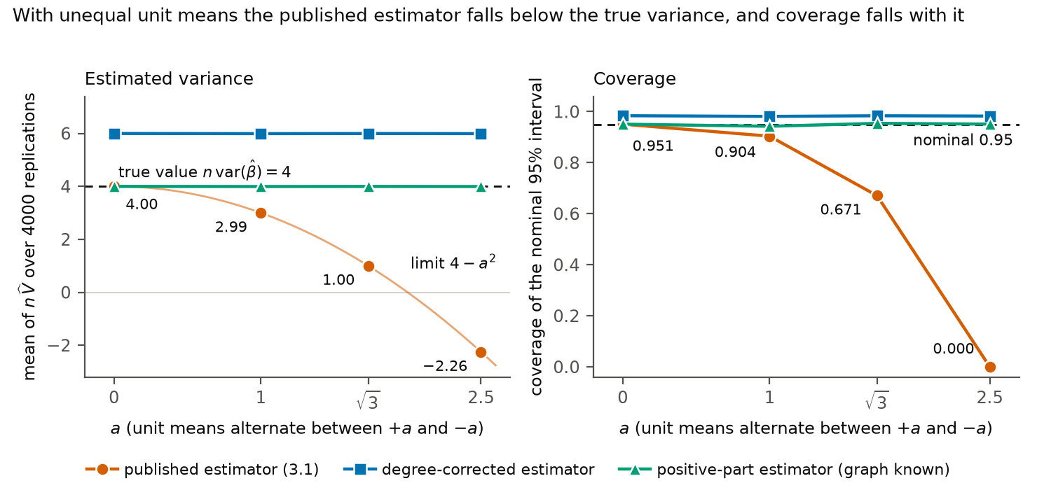
The second example consists of independent blocks of four units on a cycle. Each edge carries an independent fair sign, YiY_i is asias_i plus the two signs on the edges at ii, with s=(1,−1,1,−1)s=(1,-1,1,-1), and θi=1\theta_i=1. The covariance matrix of a block is 2I+A2I+A, every edge is known and every degree is 2. Then nvar⁡(β^)=4n\operatorname{var}(\hat\beta)=4 and nV^1(AO;Z)n\widehat V_1(A^{\mathcal O};Z) tends to 4−a24-a^2. For a=3/2a=3/2 the limit is 7/47/4, the exact mean is 7/4−12/n7/4-12/n, and the coverage of the nominal 95% interval tends to about 0.8050.805.

Exact examples that satisfy Assumptions 1, 2 and 3. Every edge is known and every degree is attained, so that Am=AOA^m=A^{\mathcal O}. The last column is the limiting coverage of the nominal 95% interval; in the second row the estimate is negative with probability tending to one.
Examplenvar⁡(β^)n\operatorname{var}(\hat\beta)Limit of nV^1(Am;Z)n\widehat V_1(A^m;Z)Coverage
Paths of three, unit means (1,−2,1)(1,-2,1)29/1529/1519/1519/150.8870.887
Paths of three, unit means (2,−4,2)(2,-4,2)29/1529/15−11/15-11/15–
Cycles of four, unit means ±3/2\pm3/2447/47/40.8050.805

Simulations of the second example, which I call example A, agree with these limits. The figure shows them for four values of aa. The next table adds example B, a difference in means on the same cycles. The units of a cycle alternate between treatment and control, YiY_i is μ\mu plus the two edge signs plus an independent unit sign, and θi=±2\theta_i=\pm2. In this example, β=0\beta=0, nvar⁡(β^)=4n\operatorname{var}(\hat\beta)=4 and the unit means are ±2μ\pm2\mu. The estimators V^1+\widehat V_1^{+}, V^Y′\widehat V_Y' and V^+\widehat V_{+} are defined in the corrected statements below. Residual centering replaces eie_i by θi\theta_i times the deviation of YiY_i from the mean of its arm.

Known graph, n=2000n=2000, 4000 replications. Example A with a=3a=\sqrt3 and example B with μ=1\mu=1; the true value nvar⁡(β^)n\operatorname{var}(\hat\beta) is 4 in both. Mean of nV^n\widehat V and coverage of the nominal 95% interval; a nonpositive variance estimate counts as a miss. Monte Carlo standard errors of the coverages are at most 0.0080.008.
EstimatorA: nV^n\widehat VA: coverageB: nV^n\widehat VB: coverage
V^1(AO)\widehat V_1(A^{\mathcal O}), as published1.000.6710.000.222
V^1+(AO)\widehat V_1^{+}(A^{\mathcal O})5.990.98416.001.000
V^Y′\widehat V_Y'15.001.00047.991.000
V^+\widehat V_{+}4.000.9549.000.997
Residual centering––4.010.950

The last table concerns the unknown graph. The maximization over compatible graphs is solved by integer programming, with n=120n=120, degree bounds di=2d_i=2 and the two examples of the previous table. With no known edge the published estimator is conservative. It fails when the known edges fix most of the graph.

Unknown graph, n=120n=120, di=2d_i=2, 1000 replications, true value 4; examples A (a=3a=\sqrt3) and B (μ=1\mu=1). The published maximal estimator V^1(Am)\widehat V_1(A^m) beside V^min⁡\widehat V_{\min}, the smaller of V^1+(A+)\widehat V_1^{+}(A^{+}) and V^Y′\widehat V_Y'. The 108 edges were drawn at random once. Coverage is computed as in the previous table. Monte Carlo standard errors of the coverages are at most 0.0160.016.
ExampleKnown edgesnV^1(Am)n\widehat V_1(A^m)CoveragenV^min⁡n\widehat V_{\min}Coverage
Anone14.901.00014.901.000
A27 of the 30 cycles2.200.8267.160.994
A108 of the 120 edges2.250.8357.210.994
Aall0.910.5875.870.977
Bnone47.761.00047.771.000
B27 of the 30 cycles4.220.84220.141.000
B108 of the 120 edges4.320.88520.241.000
Ball−0.15-0.150.33315.771.000

The simulations illustrate the limits and are not part of the argument. The term n−1δT(I+AO)δn^{-1}\delta^{\mathsf T}(I+A^{\mathcal O})\delta can also be zero or positive, and unequal unit means do not always make the published estimator anticonservative.

What survives

The following are unaffected.

  • The definitions, and the inequality V^(Am;Z)≥V^(AO;Z)\widehat V(A^m;Z)\ge\widehat V(A^{\mathcal O};Z) in every sample.
  • The programs (3.5), (3.6) and (3.8) as optimization problems.
  • The bound of order 1/n1/n on the variance of the estimator in the proof of Proposition 1, after the corrections to display (3.3) in P011-E003.
  • The central limit theorem of Lemma 2.
  • Lemma 3 and Proposition 3, which are conditional on a property of the variance estimator.

The conclusions of Proposition 2, Lemma 1 and Corollaries 2 and 4 for V^2\widehat V_2 and V^2′\widehat V_2' hold with unequal unit means, by a direct argument, although the printed proof of Proposition 2 does not (see P011-E004).

The general guarantees need qualification when unit means differ and edges are known: Proposition 1, Corollaries 1 and 3, the sentence on p. 2246, and the corresponding claims of the abstract, the introduction and the discussion. The corrected conservativeness condition below retains the original maximized estimator in additional graph and mean configurations, including sparse known edges and known graphs close to disjoint cliques. It does not remove the need for an additional condition, and homoskedasticity alone does not supply one. The heteroskedastic branch of the package computes the same estimator, and its vignette applies it to OLS coefficients with known recruitment edges (see P011-N006). The article reports no simulation or application results, so no empirical number changes. I have not established that any interval in the vignette undercovers.

Corrected

Throughout, Xi=θiYiX_i=\theta_iY_i, δi=E[Xi]−β\delta_i=\mathbb{E}[X_i]-\beta, ei=Xi−β^e_i=X_i-\hat\beta, and di′=min⁡{di,n−1}d_i'=\min\{d_i,n-1\}.

Proposition 1. Under Assumption 2, for any ϵ>0\epsilon>0,

lim⁡n→∞Pr⁡(∣nV^1(AO;Z)−nvar⁡(β^)−1nδT(I+AO)δ∣>ϵ)=0.\lim_{n\to\infty}\Pr\Bigl(\bigl|n\widehat V_1(A^{\mathcal O};Z)-n\operatorname{var}(\hat\beta)-\colorbox{#ffe58a}{$\displaystyle \tfrac1n\delta^{\mathsf T}(I+A^{\mathcal O})\delta$}\bigr|>\epsilon\Bigr)=0.

Hence the conclusion of Proposition 1 as printed holds if and only if n−1δT(I+AO)δ→0n^{-1}\delta^{\mathsf T}(I+A^{\mathcal O})\delta\to0. It holds in particular if E[θiYi]=β\mathbb{E}[\theta_iY_i]=\beta for every i∈VSi\in\mathcal V_S. In the proof, the sentence on asymptotic unbiasedness becomes E[nV^1(AO;Z)]=nvar⁡(β^)+n−1δT(I+AO)δ+O(n−1)\mathbb{E}[n\widehat V_1(A^{\mathcal O};Z)]=n\operatorname{var}(\hat\beta)+n^{-1}\delta^{\mathsf T}(I+A^{\mathcal O})\delta+O(n^{-1}).

Corollary 1: a broader sufficient condition. Retain Assumptions 1–2 and the original point estimator. Let ARA_R be the known-edge adjacency matrix. Choose fixed valid integer caps

deg⁡AO(i)≤hi≤min⁡{di,n−1},max⁡ihi≤D<∞,\deg_{A^{\mathcal O}}(i)\le h_i\le\min\{d_i,n-1\}, \qquad \max_i h_i\le D<\infty,

and define

ri=∑j(AR)ij,si=hi−ri,KR=I+AR+diag⁡(si).r_i=\sum_j(A_R)_{ij},\qquad s_i=h_i-r_i,\qquad K_R=I+A_R+\operatorname{diag}(s_i).

The original maximization may retain larger supplied caps. Let Q⪰0Q\succeq0 be fixed with ∥Q∥op=O(1)\|Q\|_{\mathrm{op}}=O(1), and write the variance inputs as

v=X−E[X]+δ+a,∥δ∥2=O(n),∥a∥2n→p0,max⁡ivi2n→p0,v=X-\mathbb{E}[X]+\delta+a,\qquad \|\delta\|^2=O(n),\qquad \frac{\|a\|^2}{n}\to_p0,\qquad \frac{\max_i v_i^2}{n}\to_p0,

where δ\delta is deterministic. Here δ\delta is the centering error for these inputs; for the published inputs v=e=X−β^1v=e=X-\hat\beta\mathbf1, it is the original E[X]−β1\mathbb{E}[X]-\beta\mathbf1. All the other input conditions then follow from Assumption 2. Define

V^(v,Q)=1n2{max⁡A∈A(Z)vT(I+A)v+vTQv}.\widehat V(v,Q)=\frac1{n^2} \left\{\max_{A\in\mathcal A(Z)}v^{\mathsf T}(I+A)v+v^{\mathsf T}Qv\right\}.

If condition (C) holds,

lim inf⁡n→∞δT(KR+Q)δn≥0,\colorbox{#ffe58a}{$\displaystyle \liminf_{n\to\infty}\frac{\delta^{\mathsf T}(K_R+Q)\delta}{n}\ge0$},

then, for every ϵ>0\epsilon>0,

lim⁡n→∞Pr⁡{nvar⁡(β^)−nV^(v,Q)>ϵ}=0.\lim_{n\to\infty}\Pr\{n\operatorname{var}(\hat\beta)-n\widehat V(v,Q)>\epsilon\}=0.

For v=ev=e and Q=0Q=0 this is the original maximized estimator. Condition (C) concerns only the relevant mean directions: if δ∈col⁡(U)\delta\in\operatorname{col}(U) and UTU=IU^{\mathsf T}U=I, it suffices that

λmin⁡{UT(KR+Q)U}≥−εn,εn→0.\lambda_{\min}\{U^{\mathsf T}(K_R+Q)U\}\ge-\varepsilon_n, \qquad \varepsilon_n\to0.

The negative eigenvalues of the full matrix need not vanish.

For Q=0Q=0, each of the following ensures (C). The first two use published centering, for which the mean deviations are uniformly bounded.

  1. There are o(n)o(n) known edges. This includes degree-only constraints, with no known edges.
  2. Deleting o(n)o(n) known edges leaves vertex-disjoint clique components. In particular, it suffices that only o(n)o(n) known edges belong to components that are not cliques. The retained clique edges may number O(n)O(n) and their caps need not be saturated. Exact disjoint cliques are a special case; overlapping cliques alone do not suffice.
  3. For every vertex, hi≥2ri−1h_i\ge2r_i-1. Then
    KR=AR+diag⁡(ri)+diag⁡(1+hi−2ri)⪰0.K_R=A_R+\operatorname{diag}(r_i) +\operatorname{diag}(1+h_i-2r_i)\succeq0.
  4. The mean deviations lie in a specified space on which KRK_R is positive semidefinite, or its smallest restricted eigenvalue tends to zero from below, as in the spectral condition above. Common transformed means, E[Xi]=β\mathbb{E}[X_i]=\beta, give δ=0\delta=0.

There is also the direct sufficient condition lim inf⁡n−1δT(I+AO)δ≥0\liminf n^{-1}\delta^{\mathsf T}(I+A^{\mathcal O})\delta\ge0, from the corrected Proposition 1. A true graph consisting of disjoint cliques satisfies this condition for every mean vector. Neither this condition nor (C) requires the mean term to tend to zero, so neither establishes the published oracle’s consistency.

Two fixed corrections after maximization. For any mean vector satisfying the input conditions, (C) holds with

Q=(−KR)+,Q=(-K_R)_+,

the negative spectral part of KRK_R with its signs reversed, since KR+Q⪰0K_R+Q\succeq0. Alternatively, let FF be a fixed set of known edges whose deletion leaves vertex-disjoint cliques, and take its Laplacian Q=LFQ=L_F. The added term is

1n2vTLFv=1n2∑{i,j}∈F(vi−vj)2.\frac1{n^2}v^{\mathsf T}L_Fv =\frac1{n^2}\sum_{\{i,j\}\in F}(v_i-v_j)^2.

There is no requirement that ∣F∣=o(n)|F|=o(n): if AR∖FA_{R\setminus F} is the remaining adjacency matrix,

KR+LF=I+AR∖F+diag⁡{si+deg⁡F(i)}⪰0.K_R+L_F=I+A_{R\setminus F} +\operatorname{diag}\{s_i+\deg_F(i)\}\succeq0.

Both choices have bounded operator norm under the stated caps. Each is added after maximization, so it preserves the maximizing graph; either may widen the variance bound.

The sufficient condition follows from a compatible-graph construction and a variance calculation. Proper-color the known graph, sort the inputs within each color and remaining-capacity class, and join consecutive groups of si+1s_i+1 vertices into cliques. The new edges respect all caps and do not duplicate known edges. The loss relative to vTKRvv^{\mathsf T}K_Rv is at most a constant depending on DD times max⁡ivi2\max_i v_i^2, which gives

nV^(v,Q)≥1nvT(KR+Q)v−op(1).n\widehat V(v,Q)\ge\frac1n v^{\mathsf T}(K_R+Q)v-o_p(1).

Put u=X−E[X]u=X-\mathbb{E}[X], Σ=cov⁡(X)\Sigma=\operatorname{cov}(X) and B=I+AOB=I+A^{\mathcal O}. If AU=AO−ARA_U=A^{\mathcal O}-A_R has degrees tit_i, then

KR−B=LU+diag⁡(si−ti)⪰0,tr⁡(BΣ)n=nvar⁡(β^).K_R-B=L_U+\operatorname{diag}(s_i-t_i)\succeq0, \qquad \frac{\operatorname{tr}(B\Sigma)}n=n\operatorname{var}(\hat\beta).

Bounded-degree dependence gives n−1uTKRu=tr⁡(KRΣ)/n+op(1)n^{-1}u^{\mathsf T}K_Ru=\operatorname{tr}(K_R\Sigma)/n+o_p(1) and ∥Σ∥op=O(1)\|\Sigma\|_{\mathrm{op}}=O(1). The deterministic mean cross term is op(1)o_p(1) after division by nn, and the input remainder aa changes the quadratic form by op(1)o_p(1) on that scale. The possibly dense correction needs no local concentration argument: uTQu≥0u^{\mathsf T}Qu\ge0. Hence

nV^(v,Q)≥nvar⁡(β^)+1nδT(KR+Q)δ+op(1),n\widehat V(v,Q)\ge n\operatorname{var}(\hat\beta) +\frac1n\delta^{\mathsf T}(K_R+Q)\delta+o_p(1),

which proves conservativeness under (C). The first two graph routes follow by bounding the adverse mean cross products by a constant times the number of exceptional known edges. The covariance and mean terms are separated in the same manner as in Yap’s Theorem 2; the graph construction and probability argument above are needed for this estimator.

Corollary 3. Given Assumptions 1–2 and the input conditions and condition (C) above, the intervals

β^±z1−α/2V^(v,Q)\hat\beta\pm z_{1-\alpha/2}\sqrt{\widehat V(v,Q)}

have at least 100(1−α)%100(1-\alpha)\% coverage for β\beta in large nn. The interval is taken to be empty when its variance estimate is negative; this event has probability tending to zero. The conclusion follows from Lemma 2 and the conservativeness bound, since nvar⁡(β^)n\operatorname{var}(\hat\beta) tends to a positive constant. It does not require consistency of the maximum or of the original oracle. The same coverage conclusion holds for the original maximized estimator under the direct mean-term condition stated above.

Section 3.2, sentence after Assumption 3. “Under condition (C) with published centering and Q=0Q=0, the general estimator V^1(Am,Z)\widehat V_1(A^m,Z) developed in Section 3.1 provides a conservative variance estimate.” The direct mean-term condition above is another sufficient qualification. Assumption 3 alone does not imply either one.

Estimators that are conservative for any unit means. For a compatible AA with degrees diA=∑jAijd_i^A=\sum_jA_{ij}, define

V^1+(A;Z)=V^1(A;Z)+1n2∑i∈VS(1−1di′)diA ei2,V^Y′(Z)=1n2∑i∈VS(1+di′) ei2,\widehat V_1^{+}(A;Z)=\widehat V_1(A;Z)+\frac1{n^2}\sum_{i\in\mathcal V_S}\Bigl(1-\frac1{d_i'}\Bigr)d_i^A\,e_i^2, \qquad \widehat V_Y'(Z)=\frac1{n^2}\sum_{i\in\mathcal V_S}(1+d_i')\,e_i^2,

where the summand of the first sum is zero when di′=0d_i'=0. Let A+A^{+} maximize V^1+(A;Z)\widehat V_1^{+}(A;Z) over A(Z)\mathcal A(Z). Given Assumption 2, for any unit means and any ϵ>0\epsilon>0,

lim⁡n→∞Pr⁡(nvar⁡(β^)−nV^>ϵ)=0\lim_{n\to\infty}\Pr\bigl(n\operatorname{var}(\hat\beta)-n\widehat V>\epsilon\bigr)=0

for V^\widehat V equal to V^1+(AO;Z)\widehat V_1^{+}(A^{\mathcal O};Z), V^1+(A+;Z)\widehat V_1^{+}(A^{+};Z), V^Y′(Z)\widehat V_Y'(Z), or the smaller of the last two. When the graph is known, the same holds for V^+(Z)=n−2eT(I+AO)+e\widehat V_{+}(Z)=n^{-2}e^{\mathsf T}(I+A^{\mathcal O})_{+}e, where (I+AO)+(I+A^{\mathcal O})_{+} is obtained from I+AOI+A^{\mathcal O} by setting its negative eigenvalues to zero. These estimators are nonnegative, and by Proposition 3 their Wald intervals have at least 100(1−α)%100(1-\alpha)\% coverage in large nn.

These statements hold for the following reason. Let CC be the covariance matrix of (X1,…,Xn)(X_1,\ldots,X_n), and let MM be a deterministic symmetric matrix whose operator norm is bounded in nn. The same derivation gives

1neTMe−nvar⁡(β^)=1n[tr⁡((M−I−AO)C)+δTMδ]+op(1).\frac1n e^{\mathsf T}Me-n\operatorname{var}(\hat\beta)=\frac1n\Bigl[\operatorname{tr}\bigl((M-I-A^{\mathcal O})C\bigr)+\delta^{\mathsf T}M\delta\Bigr]+o_p(1).

Both terms in the bracket are nonnegative when MM and M−I−AOM-I-A^{\mathcal O} are positive semidefinite. For V^1+(AO;Z)\widehat V_1^{+}(A^{\mathcal O};Z), the matrix MM is the sum of AO+diag⁡(diAO)A^{\mathcal O}+\operatorname{diag}(d_i^{A^{\mathcal O}}), whose quadratic form is ∑i<jAijO(xi+xj)2\sum_{i<j}A^{\mathcal O}_{ij}(x_i+x_j)^2, and of the nonnegative diagonal matrix diag⁡(1−diAO/di′)\operatorname{diag}(1-d_i^{A^{\mathcal O}}/d_i'), where the ratio is zero when di′=0d_i'=0. The matrix M−I−AOM-I-A^{\mathcal O} is then a nonnegative diagonal matrix. For V^Y′\widehat V_Y', since di′≥diAOd_i'\ge d_i^{A^{\mathcal O}}, I have V^Y′≥n−2eT(I+diag⁡(diAO))e\widehat V_Y'\ge n^{-2}e^{\mathsf T}(I+\operatorname{diag}(d_i^{A^{\mathcal O}}))e in every sample, and for M=I+diag⁡(diAO)M=I+\operatorname{diag}(d_i^{A^{\mathcal O}}) the matrix M−I−AOM-I-A^{\mathcal O} is the Laplacian of the graph, which is positive semidefinite. The maximum over A(Z)\mathcal A(Z) is at least the oracle value in every sample, as in the proof of Corollary 1. The display must not be applied to a matrix that is chosen from the data. The no-known-edge case also follows directly from V^Y′\widehat V_Y': if no edge is known and the bounds di′d_i' are at most DD, then 0≤nV^Y′−nV^1(Am;Z)≤B2n−1∑d=1D(3d2+2d)0\le n\widehat V_Y'-n\widehat V_1(A^m;Z)\le B^2n^{-1}\sum_{d=1}^{D}(3d^2+2d) in every sample, with B=max⁡i∣ei∣≤2c1B=\max_i|e_i|\le2c_1. If the bounds di′d_i' are not bounded in nn, the same argument applies after each bound is replaced by the smaller of di′d_i' and the least integer above c2c_2, which can only lower the maximum.

The estimator V^1+\widehat V_1^{+} is affine in AA. Program (3.6) therefore applies with the weights v^ij=eiej+(1−1/di′)ei2/2+(1−1/dj′)ej2/2\hat v_{ij}=e_ie_j+(1-1/d_i')e_i^2/2+(1-1/d_j')e_j^2/2, with 1−1/di′1-1/d_i' interpreted as zero when di′=0d_i'=0, and n2V^1+(A+;Z)=∑iei2+2w∗n^2\widehat V_1^{+}(A^{+};Z)=\sum_ie_i^2+2w^{*}, where w∗w^{*} is the optimal value. These estimators are conservative and in general not consistent. In the cycle example with a=3a=\sqrt3 and true value 4, the limits of nV^1+n\widehat V_1^{+}, nV^Y′n\widehat V_Y' and nV^+n\widehat V_{+} are 6, 15 and 4.

Regression residuals. Retain the original point estimator. For nonrandom regressors fif_i, fit YiY_i by θi2\theta_i^2-weighted least squares and use

vi=θi(Yi−fiTγ^)v_i=\theta_i(Y_i-f_i^{\mathsf T}\hat\gamma)

only in the variance estimator. Let WW have rows θifiT\theta_i f_i^{\mathsf T} and suppose rank⁡(W)=o(n)\operatorname{rank}(W)=o(n); a fixed number of regressors suffices. The conditions are met if E[Yi]=fiTγ\mathbb{E}[Y_i]=f_i^{\mathsf T}\gamma, or, more generally, if

inf⁡γ1n∑iθi2{E[Yi]−fiTγ}2⟶0.\inf_\gamma\frac1n\sum_i\theta_i^2 \{\mathbb{E}[Y_i]-f_i^{\mathsf T}\gamma\}^2\longrightarrow0.

To see the prediction rate, let PP be the orthogonal projection onto col⁡(W)\operatorname{col}(W) and μ=E[X]\mu=\mathbb{E}[X]. The transformed fitted values are PXPX, including when coefficients are not unique or some weights are zero. Since ∥Σ∥op=O(1)\|\Sigma\|_{\mathrm{op}}=O(1),

1nE∥PX−μ∥2=tr⁡(PΣ)+∥(I−P)μ∥2n≤∥Σ∥oprank⁡(W)n+inf⁡γ1n∑iθi2{E[Yi]−fiTγ}2⟶0.\begin{aligned} \frac1n\mathbb{E}\|PX-\mu\|^2 &=\frac{\operatorname{tr}(P\Sigma)+\|(I-P)\mu\|^2}{n}\\ &\le\frac{\|\Sigma\|_{\mathrm{op}}\operatorname{rank}(W)}n +\inf_\gamma\frac1n\sum_i\theta_i^2 \{\mathbb{E}[Y_i]-f_i^{\mathsf T}\gamma\}^2 \longrightarrow0. \end{aligned}

Thus v=u+δ+av=u+\delta+a with δ=(I−P)μ\delta=(I-P)\mu, a=−Pua=-Pu, ∥δ∥2/n→0\|\delta\|^2/n\to0 and ∥a∥2/n→p0\|a\|^2/n\to_p0. These bounds also imply max⁡ivi2/n→p0\max_i v_i^2/n\to_p0 and (C). Under exact specification δ=0\delta=0. No separate coefficient-convergence rate or uniformly bounded-regressor assumption is required.

More generally, any predictions m^i\hat m_i satisfying

1n∑iθi2{m^i−E[Yi]}2→p0\frac1n\sum_i\theta_i^2\{\hat m_i-\mathbb{E}[Y_i]\}^2\to_p0

can replace the weighted least-squares fit. In all these regression cases, the uncorrected true-graph residual oracle is consistent:

1nvT(I+AO)v−nvar⁡(β^)→p0.\frac1n v^{\mathsf T}(I+A^{\mathcal O})v -n\operatorname{var}(\hat\beta)\to_p0.

Indeed, ∥v−u∥2/n→p0\|v-u\|^2/n\to_p0 and ∥I+AO∥op=O(1)\|I+A^{\mathcal O}\|_{\mathrm{op}}=O(1), so replacing uu by vv changes the scaled quadratic form by op(1)o_p(1). The maximum over compatible graphs is conservative and need not be consistent. Adding QQ can likewise introduce further conservativeness. Correct specification alone does not justify arbitrary unweighted fitting under the paper’s assumptions.

Abstract. “The oracle variance estimator has an asymptotic mean term. It is consistent, at the scale of nn times the variance, if and only if that term vanishes, and it can be anticonservative otherwise. The maximized estimator has asymptotically conservative coverage under the additional sufficient conditions stated above; fixed positive semidefinite corrections and suitable regression residuals provide further repairs.” The coverage guarantees of Corollary 4 are unaffected.
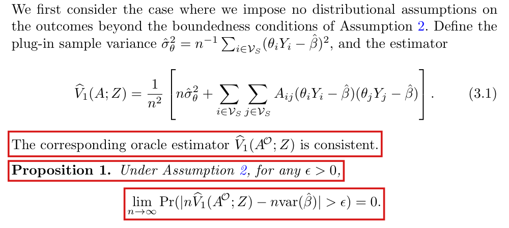

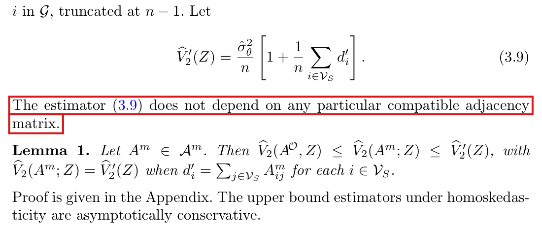
Crop of the opening of Section 3.1. It shows the definition of the plug-in sample variance and display (3.1) for the estimator V1-hat of A and Z. Red boxes mark the sentence 'The corresponding oracle estimator V1-hat(A^O; Z) is consistent.', the line 'Proposition 1. Under Assumption 2, for any epsilon > 0,' and the display stating that the limit of Pr(|n V1-hat(A^O; Z) - n var(beta-hat)| > epsilon) is 0.
Section 3.1, p. 2242 (PDF p. 5): the estimator (3.1), the sentence that calls the oracle estimator consistent, and Proposition 1. The marked statements assume Assumption 2 only.
Crop of the first four lines of page 2243. A red box marks the sentence 'Asymptotic unbiasedness follows directly from linearity of expectations and var(beta-hat) = O(n^-1).', which runs over two lines.
Proof of Proposition 1, p. 2243 (PDF p. 6), first paragraph. The marked sentence is the step that omits the products of the deviations of the unit means.
Crop of three paragraphs. A red box marks the statement 'Corollary 1. Given Assumption 2, the limit as n tends to infinity of Pr(n var(beta-hat) - n V1-hat(A^m; Z) > epsilon) = 0 for any epsilon > 0.' The paragraph before it says that as n grows large the variance estimate V1-hat(A^m, Z) is conservative.
Corollary 1, p. 2245 (PDF p. 8), with the paragraphs before and after it.
Crop of Assumption 3 (Homoskedasticity) and the four lines after it. A red box marks the sentence 'Under homoskedasticity, the general estimator V1-hat(A^m, Z) developed in Section 3.1 provides a conservative variance estimate.'
Assumption 3 and the first sentence after it, p. 2246 (PDF p. 9). The marked sentence claims that the general estimator is conservative under homoskedasticity.
Crop of a three-line paragraph and Corollaries 3 and 4. A red box marks 'Corollary 3. Given Assumption 2, confidence intervals formed as beta-hat plus or minus z times the square root of V1-hat(A^m) have at least 100(1 - alpha) percent coverage for beta in large n.' Corollary 4, for V2-hat and V2-hat-prime under Assumptions 2 and 3, is not marked.
Corollaries 3 and 4, p. 2248 (PDF p. 11). Corollary 3, marked, is the coverage claim for the general estimator.
Two line charts with the same horizontal axis, the value a at 0, 1, the square root of 3 and 2.5. Left panel, mean of n times the variance estimate: orange circles for the published estimator at 4.00, 2.99, 1.00 and minus 2.26, lying on the curve 4 minus a squared; a dashed line at the true value 4; blue squares for the degree-corrected estimator near 6; green triangles for the positive-part estimator near 4. Right panel, coverage of the nominal 95 percent interval: the published estimator at 0.951, 0.904, 0.671 and 0.000; the two corrected estimators between 0.94 and 0.99, close to the dashed nominal line at 0.95.
Simulation of the cycle example with a known graph, n=2000n=2000, 4000 replications for each value of aa. Left: the mean of nV^n\widehat V for the published estimator (3.1) follows its limit 4−a24-a^2 and leaves the true value 4, while the degree-corrected estimator V^1+\widehat V_1^{+} stays near 6 and the positive-part estimator V^+\widehat V_{+} near 4. Right: the coverage of the nominal 95% interval built on the published estimator falls from 0.951 at a=0a=0 to 0.904, 0.671 and 0.000; the two corrected estimators cover at 0.94 or more.
My comment and the history of this entry

I investigated this, in part with help from an LLM. I agree, but want to suggest a more broad type of correction. The following is LLM-generated output, generated at my supervision:

An additional condition for conservative inference

Retain Assumptions 1–2. Write Xi=θiYiX_i=\theta_iY_i, and let ARA_R be the known-edge adjacency matrix. Choose fixed integer caps deg⁡AO(i)≤hi≤min⁡{di,n−1}\deg_{A^{\mathcal O}}(i)\le h_i\le\min\{d_i,n-1\}, with max⁡ihi≤D<∞\max_i h_i\le D<\infty; the original maximization may retain larger supplied caps. Define

ri=∑j(AR)ij,si=hi−ri,KR=I+AR+diag⁡(si).r_i=\sum_j(A_R)_{ij},\qquad s_i=h_i-r_i,\qquad K_R=I+A_R+\operatorname{diag}(s_i).

Thus sis_i is the capacity left for unknown edges. Let vv be the variance inputs, and optionally add a fixed correction Q⪰0Q\succeq0, with ∥Q∥op=O(1)\|Q\|_{\mathrm{op}}=O(1):

V^=1n2max⁡A∈A(Z)v⊤(I+A)v+1n2v⊤Qv.\widehat V =\frac1{n^2}\max_{A\in\mathcal A(Z)}v^\top(I+A)v +\frac1{n^2}v^\top Qv.

For the published estimator, v=X−β^1v=X-\hat\beta\mathbf1 and Q=0Q=0. Regression alternatives below change the variance inputs and retain the original point estimator.

Additional condition. Write v=X−E[X]+δ+av=X-E[X]+\delta+a, where δ\delta is deterministic, ∥δ∥2=O(n)\|\delta\|^2=O(n), ∥a∥2/n→p0\|a\|^2/n\to_p0, and max⁡ivi2/n→p0\max_i v_i^2/n\to_p0. Require

lim inf⁡n→∞δ⊤(KR+Q)δn≥0.(C)\boxed{\displaystyle \liminf_{n\to\infty}\frac{\delta^\top(K_R+Q)\delta}{n}\ge0.} \tag{C}

For published centering, δ=E[X]−β1\delta=E[X]-\beta\mathbf1, and the other requirements follow from Assumption 2. A sufficient spectral certificate, when δ∈col⁡(U)\delta\in\operatorname{col}(U) and U⊤U=IU^\top U=I, is

λmin⁡{U⊤(KR+Q)U}≥−εn,εn→0.\lambda_{\min}\{U^\top(K_R+Q)U\}\ge-\varepsilon_n, \qquad \varepsilon_n\to0.

Condition (C) gives asymptotic variance conservativeness and at-least-nominal Wald coverage. It restricts the relevant mean directions; it does not require the full matrix's negative eigenvalues to vanish.

The following are sufficient routes. The first two use published centering, whose mean deviations are uniformly bounded.

  • Few known edges. The number of known edges is o(n)o(n). This includes degree-only constraints, with no known edges.
  • The known graph is nearly a union of disjoint cliques. Deleting o(n)o(n) known edges leaves vertex-disjoint clique components. A simple sufficient case is that only o(n)o(n) known edges belong to components that are not cliques. The remaining clique edges may number O(n)O(n), and their degree caps need not be saturated. Exact disjoint cliques are a special case; overlapping cliques alone do not suffice.
  • Enough remaining degree capacity. For every vertex, hi≥2ri−1h_i\ge2r_i-1. Then

    KR=AR+diag⁡(ri)+diag⁡(1+hi−2ri)⪰0.K_R=A_R+\operatorname{diag}(r_i) +\operatorname{diag}(1+h_i-2r_i)\succeq0.
  • A compatible mean space. The possible mean deviations lie in a specified space col⁡(U)\operatorname{col}(U), and U⊤KRUU^\top K_RU is positive semidefinite, or its minimum eigenvalue tends to zero from below. Common transformed means, E[Xi]=βE[X_i]=\beta, give δ=0\delta=0.
  • An explicit correction is added. One universal choice is Q=(−KR)+Q=(-K_R)_+, the negative spectral part of KRK_R with its signs reversed. Alternatively, choose a known-edge set FF whose deletion leaves vertex-disjoint cliques, and add

    1n2∑{i,j}∈F(vi−vj)2.\frac1{n^2}\sum_{\{i,j\}\in F}(v_i-v_j)^2.

    This uses Q=LFQ=L_F, the Laplacian of the deleted edges; FF need not be o(n)o(n). Both corrections are added after maximization and preserve the original maximizing graph.

  • Residuals from a well-specified regression. Suppose E[Yi]=fi⊤γE[Y_i]=f_i^\top\gamma, with nonrandom regressors. Fit by θi2\theta_i^2-weighted least squares and use vi=θi(Yi−fi⊤γ^)v_i=\theta_i(Y_i-f_i^\top\hat\gamma). It is enough that the transformed design WW, with rows θifi⊤\theta_i f_i^\top, has rank o(n)o(n); a fixed number of regressors suffices. The fitted weighted means have average squared prediction error tending to zero, so (C) holds with δ=0\delta=0.
  • Residuals from a nearly well-specified regression. Use the same fit, require rank⁡(W)=o(n)\operatorname{rank}(W)=o(n), and assume

    inf⁡γ1n∑iθi2{E[Yi]−fi⊤γ}2⟶0.\inf_\gamma\frac1n\sum_i\theta_i^2 \{E[Y_i]-f_i^\top\gamma\}^2\longrightarrow0.

    The remaining weighted mean error has ∥δ∥2/n→0\|\delta\|^2/n\to0, which implies (C). More generally, either residual case works whenever

    1n∑iθi2{m^i−E[Yi]}2→p0.\frac1n\sum_i\theta_i^2 \{\hat m_i-E[Y_i]\}^2\to_p0.

The regression cases also give consistency of the true-graph residual oracle. The maximized bound is conservative and need not be consistent. Correct specification alone is insufficient for arbitrary unweighted fitting under the paper's assumptions.

Why this works. Proper-color the known graph, then form sorted cliques separately within each color and remaining-capacity class. This gives a compatible graph and establishes

nV^≥1nv⊤(KR+Q)v−op(1).n\widehat V\ge\frac1n v^\top(K_R+Q)v-o_p(1).

Moreover, KR−(I+AO)K_R-(I+A^{\mathcal O}) is the Laplacian of the unknown true edges plus a nonnegative diagonal matrix. Its covariance contribution is therefore nonnegative; (C) controls the remaining mean contribution. The covariance/mean separation is inspired by Yap's Theorem 2.

Updated after LLMs rendered their decision.

  1. Classification before my review (the classification when the audit was first completed, before I reviewed it): Critical error.
  2. I commented.
  3. Independent evaluation. Incorporated. The correction was broadened to include the additional condition in my comment and the other sufficient routes to conservative inference that the independent check established. The entry remains Critical: these conditions do not restore the paper’s original unrestricted guarantees.

Moderate (2)

A real substantive error with limited reach.

The proof of Proposition 2 rests on the consistency of an auxiliary estimator, which can fail when the means E[θiYi]E[\theta_iY_i] differ across units; Proposition 2 itself holds under Assumptions 2 and 3 by a direct one-sided argument.

Proof of Proposition 2, p. 2246 (PDF p. 9)

See also under Formal statements (Lean): P011-T11, P011-T12, P011-T19, P011-T34, P011-T36

As printed

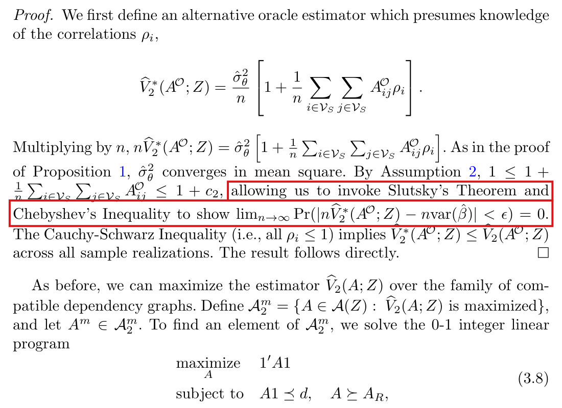
Proof. We first define an alternative oracle estimator which presumes knowledge of the correlations ρi\rho_i,

V^2∗(AO;Z)=σ^θ2n[1+1n∑i∈VS∑j∈VSAijOρi].\widehat V_2^*(A^{\mathcal O};Z)=\frac{\hat\sigma_\theta^2}{n}\left[1+\frac1n\sum_{i\in\mathcal V_S}\sum_{j\in\mathcal V_S}A^{\mathcal O}_{ij}\rho_i\right].

Multiplying by nn, nV^2∗(AO;Z)=σ^θ2[1+1n∑i∈VS∑j∈VSAijOρi]n\widehat V_2^*(A^{\mathcal O};Z)=\hat\sigma_\theta^2\left[1+\frac1n\sum_{i\in\mathcal V_S}\sum_{j\in\mathcal V_S}A^{\mathcal O}_{ij}\rho_i\right]. As in the proof of Proposition 1, σ^θ2\hat\sigma_\theta^2 converges in mean square. By Assumption 2, 1≤1+1n∑i∈VS∑j∈VSAijO≤1+c21\le1+\frac1n\sum_{i\in\mathcal V_S}\sum_{j\in\mathcal V_S}A^{\mathcal O}_{ij}\le1+c_2, allowing us to invoke Slutsky’s Theorem and Chebyshev’s Inequality to show lim⁡n→∞Pr⁡(∣nV^2∗(AO;Z)−nvar⁡(β^)∣<ϵ)=0\colorbox{#ffe58a}{$\lim_{n\to\infty}\Pr(|n\widehat V_2^*(A^{\mathcal O};Z)-n\operatorname{var}(\hat\beta)|<\epsilon)=0$}. The Cauchy-Schwarz Inequality (i.e., all ρi≤1\rho_i\le1) implies V^2∗(AO;Z)≤V^2(AO;Z)\widehat V_2^*(A^{\mathcal O};Z)\le\widehat V_2(A^{\mathcal O};Z) across all sample realizations. The result follows directly.

The problem

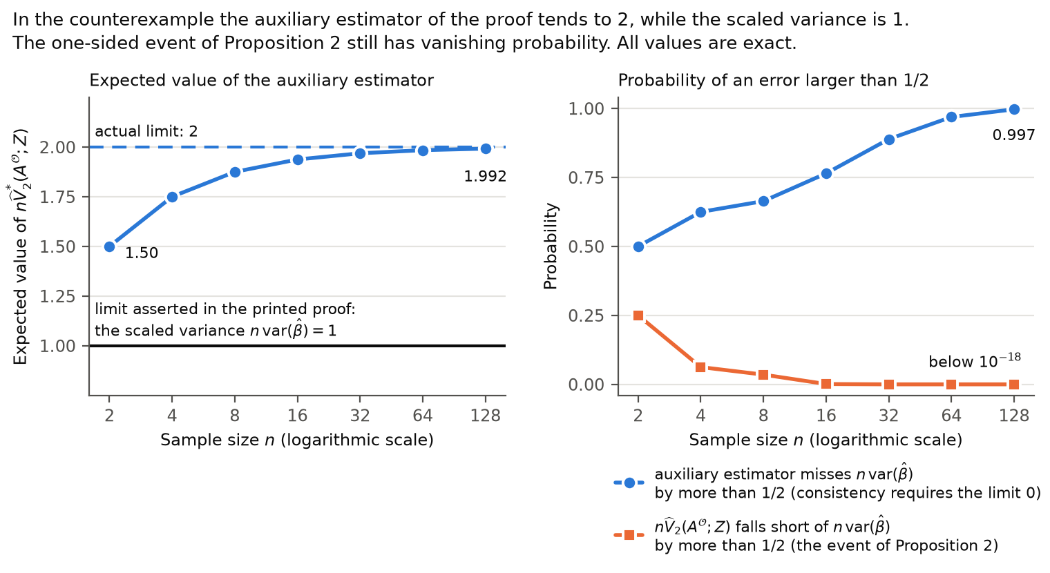
The proof introduces an auxiliary estimator V^2∗(AO;Z)\widehat V_2^*(A^{\mathcal O};Z) and asserts that nV^2∗(AO;Z)n\widehat V_2^*(A^{\mathcal O};Z) is consistent for nvar⁡(β^)n\operatorname{var}(\hat\beta). It then passes to V^2(AO;Z)\widehat V_2(A^{\mathcal O};Z) by the inequality V^2∗(AO;Z)≤V^2(AO;Z)\widehat V_2^*(A^{\mathcal O};Z)\le\widehat V_2(A^{\mathcal O};Z). The consistency is false in general under Assumptions 2 and 3. Definition 3 requires only that the average of the means E[θiYi]E[\theta_iY_i] equal β\beta, and Assumption 3 equates the variances of the θiYi\theta_iY_i, not their means. Let δi=E[θiYi]−β\delta_i=E[\theta_iY_i]-\beta and Mn=n−1∑i∈VSδi2M_n=n^{-1}\sum_{i\in\mathcal V_S}\delta_i^2. Since the sample variance σ^θ2\hat\sigma_\theta^2 is centered at the single value β^\hat\beta, it tracks the common variance of the θiYi\theta_iY_i plus MnM_n, and not the common variance alone. In the example below Mn→1M_n\to1, and nV^2∗(AO;Z)n\widehat V_2^*(A^{\mathcal O};Z) tends to 22 while nvar⁡(β^)n\operatorname{var}(\hat\beta) tends to 11. In this example, the sentence that σ^θ2\hat\sigma_\theta^2 “converges in mean square” is correct; the error lies in the limit that the next sentence assigns to the estimator. The cause is the one described in P011-E001. The marked display also carries a reversed inequality sign (P011-E005), and the proof writes the correlations with a single index (P011-E006). After both are corrected, the consistency still fails.

Evidence an exact counterexample

I use an exact counterexample. Let ε1,ε2,…\varepsilon_1,\varepsilon_2,\ldots be independent random variables such that Pr⁡(εi=1)=Pr⁡(εi=−1)=1/2\Pr(\varepsilon_i=1)=\Pr(\varepsilon_i=-1)=1/2, and let Yi=μi+εiY_i=\mu_i+\varepsilon_i with μi=2\mu_i=2 for odd ii and μi=0\mu_i=0 for even ii. At sample size nn let θi=n/(2⌈n/2⌉)\theta_i=n/(2\lceil n/2\rceil) for every ii, let β=1\beta=1, and let the graph have no edges, with every vertex observed. Then E[β^]=1E[\hat\beta]=1, ∣θiYi−β∣≤2|\theta_iY_i-\beta|\le2, every degree is zero, ∣θi∣≤1|\theta_i|\le1, var⁡(θiYi)=θi2\operatorname{var}(\theta_iY_i)=\theta_i^2 is the same for all ii, and nvar⁡(β^)=θ12→1n\operatorname{var}(\hat\beta)=\theta_1^2\to1. Assumptions 2 and 3 hold with c1=2c_1=2, c2=1c_2=1, c3=1c_3=1 and c4=2c_4=2. Since AO=0A^{\mathcal O}=0, I have nV^2∗(AO;Z)=nV^2(AO;Z)=σ^θ2n\widehat V_2^*(A^{\mathcal O};Z)=n\widehat V_2(A^{\mathcal O};Z)=\hat\sigma_\theta^2, whatever the correlations are taken to be. For even nn the weights equal 11 and Mn=1M_n=1, and a direct computation gives

E[(σ^θ2−2)2]=4n+3n2−2n3.E\bigl[(\hat\sigma_\theta^2-2)^2\bigr]=\frac4n+\frac3{n^2}-\frac2{n^3}.

Along even nn, this shows that nV^2∗(AO;Z)→2n\widehat V_2^*(A^{\mathcal O};Z)\to2 in mean square, while nvar⁡(β^)=1n\operatorname{var}(\hat\beta)=1. Markov’s inequality then implies that

Pr⁡(∣nV^2∗(AO;Z)−nvar⁡(β^)∣>1/2)≥1−4(4n+3n2−2n3)→1.\Pr\bigl(|n\widehat V_2^*(A^{\mathcal O};Z)-n\operatorname{var}(\hat\beta)|>1/2\bigr)\ge1-4\Bigl(\frac4n+\frac3{n^2}-\frac2{n^3}\Bigr)\to1 .

For odd nn, I find Mn→1M_n\to1 and the same two limits by the same computation. An enumeration of all outcomes in exact arithmetic agrees with these formulas for the sample sizes in the table.

Exact values in the counterexample (the last two columns are rounded).
nnE[nV^2∗(AO;Z)]E[n\widehat V_2^*(A^{\mathcal O};Z)]nvar⁡(β^)n\operatorname{var}(\hat\beta)Pr⁡(∣nV^2∗−nvar⁡(β^)∣>1/2)\Pr(|n\widehat V_2^*-n\operatorname{var}(\hat\beta)|>1/2)Pr⁡(nvar⁡(β^)−nV^2>1/2)\Pr(n\operatorname{var}(\hat\beta)-n\widehat V_2>1/2)
223/23/2110.50000.50000.25000.2500
8815/815/8110.66410.66410.03520.0352
323263/3263/32110.88870.88876.3×10−66.3\times10^{-6}
128128255/128255/128110.99700.99702.6×10−192.6\times10^{-19}

Note that the last column is the probability of the event of Proposition 2, which tends to 00 as the proposition asserts. Unequal means do not always destroy the consistency. If μ1=2\mu_1=2, μ2=0\mu_2=0 and μi=1\mu_i=1 for i≥3i\ge3, with θi=1\theta_i=1 for n≥2n\ge2, then Mn=2/nM_n=2/n and E[(nV^2∗(AO;Z)−nvar⁡(β^))2]=11/n2−2/n3→0E[(n\widehat V_2^*(A^{\mathcal O};Z)-n\operatorname{var}(\hat\beta))^2]=11/n^2-2/n^3\to0. The replacement proof below is a derivation, and each of its steps is given there.

What survives

Proposition 2 holds as stated, with no added assumption, and Lemma 1 and Corollaries 2 and 4 keep their conclusions. The estimators (3.7) and (3.9), program (3.8) and the software are unaffected, since the auxiliary estimator appears only in this proof. This correction does not restore Proposition 1 or Corollaries 1 and 3, which are the subject of P011-E001.

Corrected

The statement is unchanged: given Assumptions 2 and 3, lim⁡n→∞Pr⁡(nvar⁡(β^)−nV^2(AO;Z)>ϵ)=0\lim_{n\to\infty}\Pr(n\operatorname{var}(\hat\beta)-n\widehat V_2(A^{\mathcal O};Z)>\epsilon)=0 for any ϵ>0\epsilon>0. I replace the proof by the following.

Proof. Let Xi=θiYiX_i=\theta_iY_i and δi=E[Xi]−β\delta_i=E[X_i]-\beta, and let σn2=var⁡(Xi)\sigma_n^2=\operatorname{var}(X_i) be the common variance of Assumption 3 at sample size nn. Define

Mn=1n∑i∈VSδi2≥0,gn=1+1n∑i∈VS∑j∈VSAijO,Un=1n∑i∈VS(Xi−β)2,Rn=σ^θ2−σn2−Mn.\begin{aligned} M_n&=\frac1n\sum_{i\in\mathcal V_S}\delta_i^2\ge0, &\qquad g_n&=1+\frac1n\sum_{i\in\mathcal V_S}\sum_{j\in\mathcal V_S}A^{\mathcal O}_{ij},\\ U_n&=\frac1n\sum_{i\in\mathcal V_S}(X_i-\beta)^2, &\qquad R_n&=\hat\sigma_\theta^2-\sigma_n^2-M_n . \end{aligned}

By Assumption 2, ∣Xi−β∣≤c1|X_i-\beta|\le c_1 and 1≤gn≤1+c21\le g_n\le1+c_2. Since E[(Xi−β)2]=σn2+δi2E[(X_i-\beta)^2]=\sigma_n^2+\delta_i^2, it follows that E[Un]=σn2+MnE[U_n]=\sigma_n^2+M_n. For i≠ji\ne j with AijO=0A^{\mathcal O}_{ij}=0, the variables XiX_i and XjX_j are independent, so that cov⁡((Xi−β)2,(Xj−β)2)=0\operatorname{cov}((X_i-\beta)^2,(X_j-\beta)^2)=0 and cov⁡(Xi,Xj)=0\operatorname{cov}(X_i,X_j)=0. At most n(1+c2)n(1+c_2) ordered pairs (i,j)(i,j) have i=ji=j or AijO=1A^{\mathcal O}_{ij}=1, and for such a pair the two covariances are at most c14c_1^4 and c12c_1^2 in absolute value. Hence

var⁡(Un)≤(1+c2)c14n,E[(β^−β)2]=var⁡(β^)≤(1+c2)c12n,\operatorname{var}(U_n)\le\frac{(1+c_2)c_1^4}{n},\qquad E[(\hat\beta-\beta)^2]=\operatorname{var}(\hat\beta)\le\frac{(1+c_2)c_1^2}{n},

where the equality uses E[β^]=βE[\hat\beta]=\beta. Since ∣β^−β∣≤c1|\hat\beta-\beta|\le c_1, this gives E[(β^−β)4]≤(1+c2)c14/nE[(\hat\beta-\beta)^4]\le(1+c_2)c_1^4/n. The identity σ^θ2=Un−(β^−β)2\hat\sigma_\theta^2=U_n-(\hat\beta-\beta)^2 gives Rn=(Un−E[Un])−(β^−β)2R_n=(U_n-E[U_n])-(\hat\beta-\beta)^2, and therefore

E[Rn2]≤2var⁡(Un)+2E[(β^−β)4]≤4(1+c2)c14n.E[R_n^2]\le2\operatorname{var}(U_n)+2E[(\hat\beta-\beta)^4]\le\frac{4(1+c_2)c_1^4}{n}.

By the Cauchy–Schwarz inequality and Assumption 3, cov⁡(Xi,Xj)≤σn2\operatorname{cov}(X_i,X_j)\le\sigma_n^2 for all ii and jj, and cov⁡(Xi,Xj)=0\operatorname{cov}(X_i,X_j)=0 when i≠ji\ne j and AijO=0A^{\mathcal O}_{ij}=0. Hence

nvar⁡(β^)=1n∑i∈VS∑j∈VScov⁡(Xi,Xj)≤σn2gn.n\operatorname{var}(\hat\beta)=\frac1n\sum_{i\in\mathcal V_S}\sum_{j\in\mathcal V_S}\operatorname{cov}(X_i,X_j)\le\sigma_n^2g_n .

By (3.7), nV^2(AO;Z)=gnσ^θ2=gn(σn2+Mn+Rn)n\widehat V_2(A^{\mathcal O};Z)=g_n\hat\sigma_\theta^2=g_n(\sigma_n^2+M_n+R_n). Since Mn≥0M_n\ge0,

nvar⁡(β^)−nV^2(AO;Z)≤−gn(Mn+Rn)≤(1+c2)∣Rn∣.\colorbox{#ffe58a}{$\displaystyle n\operatorname{var}(\hat\beta)-n\widehat V_2(A^{\mathcal O};Z)\le-g_n(M_n+R_n)\le(1+c_2)|R_n|$} .

By Markov’s inequality, for every ϵ>0\epsilon>0,

Pr⁡(nvar⁡(β^)−nV^2(AO;Z)>ϵ)≤(1+c2)2E[Rn2]ϵ2≤4(1+c2)3c14nϵ2→0.\Pr\bigl(n\operatorname{var}(\hat\beta)-n\widehat V_2(A^{\mathcal O};Z)>\epsilon\bigr)\le\frac{(1+c_2)^2E[R_n^2]}{\epsilon^2}\le\frac{4(1+c_2)^3c_1^4}{n\epsilon^2}\to0 .

The argument uses no auxiliary estimator and no correlations. It needs no condition on the means beyond E[β^]=βE[\hat\beta]=\beta, and no limit for σn2\sigma_n^2 or MnM_n.

Crop of the proof of Proposition 2, followed by the paragraph that introduces program (3.8). Red boxes mark the words 'allowing us to invoke Slutsky's Theorem and Chebyshev's Inequality to show' and the limit that follows them: the limit, as n tends to infinity, of the probability that the absolute value of n V 2 star of A O, Z minus n var of beta hat is less than epsilon, set equal to 0.
Proof of Proposition 2, p. 2246 (PDF p. 9). The marked sentence asserts that nV^2∗(AO;Z)n\widehat V_2^*(A^{\mathcal O};Z) consistently estimates nvar⁡(β^)n\operatorname{var}(\hat\beta).
Two line charts against the sample size n, on a logarithmic scale from 2 to 128. In the left chart the expected value of n V 2 star rises from 1.50 at n = 2 to 1.992 at n = 128 and approaches a dashed line at 2, labelled actual limit; a solid line at 1 is labelled as the limit asserted in the printed proof, the scaled variance. In the right chart the probability that n V 2 star misses the scaled variance by more than one half rises from 0.5 to 0.997, and the probability that n V 2 falls short of the scaled variance by more than one half falls from 0.25 to below 10 to the power minus 18.
Exact values in the counterexample, for n=2,4,8,16,32,64,128n=2,4,8,16,32,64,128. Left: the expected value of nV^2∗(AO;Z)n\widehat V_2^*(A^{\mathcal O};Z), against the limit nvar⁡(β^)=1n\operatorname{var}(\hat\beta)=1 that the printed proof asserts. Right: the probability that nV^2∗(AO;Z)n\widehat V_2^*(A^{\mathcal O};Z) differs from nvar⁡(β^)n\operatorname{var}(\hat\beta) by more than 1/21/2, and the probability of the event of Proposition 2 with ϵ=1/2\epsilon=1/2. The graph of the example has no edges, so the auxiliary estimator and V^2(AO;Z)\widehat V_2(A^{\mathcal O};Z) coincide.

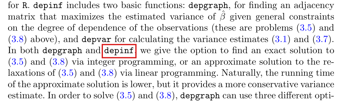
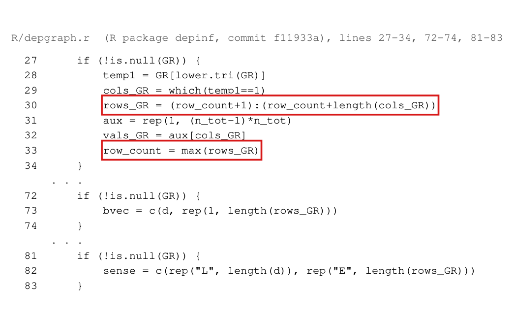
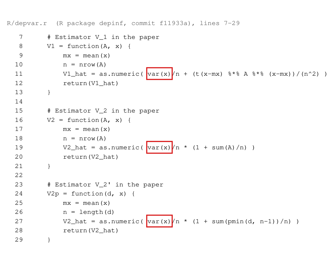
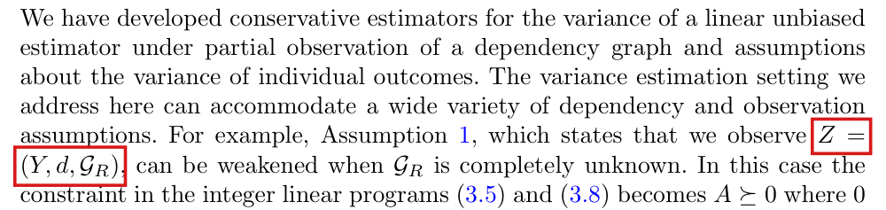
The package vignette applies the general estimator V^1\widehat V_1, with raw outcomes and known recruitment edges, to four least-squares coefficients, and the package describes the result as conservative; the paper’s assumptions alone do not justify that guarantee for these calls, and the analyses in “Section 5 of the paper” that the vignette says it replicates are not in the published article.

Acknowledgement, p. 2249 (PDF p. 12); Section 5, p. 2248 (PDF p. 11); equation (3.1) and Proposition 1, p. 2242 (PDF p. 5). Package depinf: vignettes/replication.Rmd, lines 15 and 100–105; README.md, line 3

See also under Formal statements (Lean): P011-T15, P011-T16, P011-T35

As printed

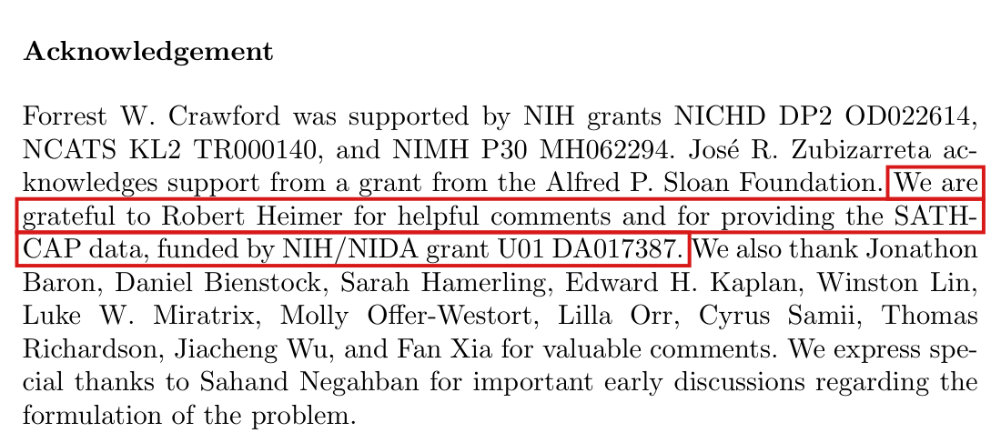
Acknowledgement, p. 2249: “We are grateful to Robert Heimer for helpful comments and for providing the SATHCAP data, funded by NIH/NIDA grant U01 DA017387.”

vignettes/replication.Rmd, line 15: “In this vignette, we replicate the main analyses in Section 5 of the paper.”

vignettes/replication.Rmd, lines 100 and 101 (line 101 is broken here to fit the page); lines 102 to 104 repeat the call for coefficients 2 to 4, and line 105 collects the four values as col5:

# V1, some known dependenciesb1 = sqrt(depvar(Y, Theta[1, ]*n, d, GR, case = "heteroskedastic",solver = "gurobi", approximate = 0)$V_hat)\begin{aligned} &\texttt{\# V1, some known dependencies}\\ &\texttt{b1 = sqrt(depvar(}\colorbox{#ffe58a}{$\displaystyle \texttt{Y}$}\texttt{, Theta[1, ]*n, d, GR, case = "heteroskedastic",}\\ &\qquad\texttt{solver = "gurobi", approximate = 0)\$V\_hat)} \end{aligned}

README.md, line 3: “The primary function, depvar, produces conservative variance estimates for generic linear unbiased estimators”

The problem

The published article has no empirical section. Its Section 5 is the Discussion, and the SATHCAP data appear only in the Acknowledgement, which is correct as it stands. The analysis of these data is in the vignette of the package that Appendix B names as the implementation of the method. The package is dated 20 January 2017 and cites the 2017 preprint. The words “Section 5 of the paper” may refer to an earlier version, which I could not obtain.

The vignette regresses HIV status on three covariates for n=522n=522 respondents. It computes standard errors for the four coefficients from V^1\widehat V_1 with the 468 known recruitment edges, and it passes the raw outcomes YiY_i with the weights θi=n[(X′X)−1X′]ji\theta_i=n[(X'X)^{-1}X']_{ji}. Known edges and unequal transformed means are allowed here, so the paper’s unqualified guarantee for V^1\widehat V_1 is not available (P011-E001). For a regression coefficient the means E[θiYi]E[\theta_iY_i] can differ across units. Let hi=E[θiYi]−βh_i=E[\theta_iY_i]-\beta. Under Assumption 2 the oracle estimator satisfies

nV^1(AO;Z)=nvar⁡(β^)+1n h′(I+AO)h+op(1),n\widehat V_1(A^{\mathcal O};Z)=n\operatorname{var}(\hat\beta)+\frac1n\,h'(I+A^{\mathcal O})h+o_p(1),

and the quadratic form can have either sign. If the added term has a negative limit and the known edges force a unique graph, the maximal compatible estimator is too small as well. The standard errors that the vignette computes in this way therefore carry no guarantee from the paper’s assumptions alone, and the README’s unrestricted description does not hold for V^1\widehat V_1. The broader condition (C) in P011-E001 supplies additional ways to justify the original maximized estimator, but its graph, capacity or mean restrictions have not been established for this application. One symptom is that these standard errors change when a constant is added to every outcome, although the slope estimates and the residuals do not.

Evidence an exact counterexample

I base this correction on an exact counterexample, a derivation and a recalculation.

For the expansion, let ui=θiYi−E[θiYi]u_i=\theta_iY_i-E[\theta_iY_i], δ=β^−β\delta=\hat\beta-\beta and B=I+AOB=I+A^{\mathcal O}, so that nV^1(AO;Z)=n−1(u+h−δ1)′B(u+h−δ1)n\widehat V_1(A^{\mathcal O};Z)=n^{-1}(u+h-\delta\mathbf{1})'B(u+h-\delta\mathbf{1}). Since the weighted outcomes and the degrees are bounded, I have var⁡(δ)=O(n−1)\operatorname{var}(\delta)=O(n^{-1}), and replacing δ\delta by 00 changes the expression by op(1)o_p(1). Next, n−1E[u′Bu]=nvar⁡(β^)n^{-1}E[u'Bu]=n\operatorname{var}(\hat\beta), because outcomes that are not adjacent are independent. The cross term has mean zero, E[u′Bh]=0E[u'Bh]=0. The terms n−1u′Bun^{-1}u'Bu and n−1u′Bhn^{-1}u'Bh have variance O(n−1)O(n^{-1}). By Chebyshev’s inequality, I obtain the expansion.

For the counterexample, let n=4kn=4k and take kk independent blocks. Each block is a star with a center and three leaves. All three edges are known and the degrees are (3,1,1,1)(3,1,1,1), which leaves the true graph as the only compatible one. Within a block let the covariate be x=(3,−1,−1,−1)x=(3,-1,-1,-1), let the outcomes L1,L2,L3L_1,L_2,L_3 of the leaves be independent with Pr⁡(Lj=1)=1/4\Pr(L_j=1)=1/4 and Pr⁡(Lj=0)=3/4\Pr(L_j=0)=3/4, and let the outcome of the center equal 11 with conditional probability 3/4+(1/12)∑j=13(Lj−1/4)3/4+(1/12)\sum_{j=1}^3(L_j-1/4) and 00 otherwise. Then E[Yi]=3/8+xi/8E[Y_i]=3/8+x_i/8, that is, the linear model is correct. The least-squares intercept is the sample mean, with θi=1\theta_i=1 and β=3/8\beta=3/8. Assumption 2 holds with c1=1c_1=1, c2=3c_2=3, c3=27/128c_3=27/128 and c4=2c_4=2. In each block h=(3/8,−1/8,−1/8,−1/8)h=(3/8,-1/8,-1/8,-1/8) and h′(I+AO)h=−3/32h'(I+A^{\mathcal O})h=-3/32, that is, −3/128-3/128 per observation. A computation with the 16 outcomes of a block in exact arithmetic gives nvar⁡(β^)=27/128n\operatorname{var}(\hat\beta)=27/128 and nV^1→3/16n\widehat V_1\to3/16 in probability, for the oracle estimator, the maximal compatible estimator and the relaxed estimator alike. For ϵ=3/256\epsilon=3/256, the probability in Corollary 1 tends to 11 and not to 00. The limiting coverage of the nominal 100(1−α)%100(1-\alpha)\% interval is 2Φ(z1−α/28/9)−12\Phi(z_{1-\alpha/2}\sqrt{8/9})-1, which is below 1−α1-\alpha. A second design shows that the bias can be positive.

Exact limits for the least-squares intercept in the two block designs.
Covariate in a blocknvar⁡(β^)n\operatorname{var}(\hat\beta)Limit of nV^1n\widehat V_1Ratio
x=(3,−1,−1,−1)x=(3,-1,-1,-1)27/12827/1283/163/168/98/9
x=(0,1,−1,0)x=(0,1,-1,0)47/19247/19253/19253/19253/4753/47

For the recalculation, I used the package’s data and functions, with the linear relaxation solved by GLPK and the 468 known edges imposed. The standard error of the hcv coefficient from V^1\widehat V_1 changes as follows when a constant is added to every outcome, while the estimate and the residuals do not change.

The hcv coefficient in the vignette’s regression, with a constant added to every outcome.
Constant addedEstimateStandard error from V^1\widehat V_1
000.38090.38090.15950.1595
110.38090.38090.50250.5025
10100.38090.38093.87003.8700

The vignette’s table was computed with Gurobi in integer mode, which was not available. Its printed value for this coefficient is 0.159516630.15951663. Sensitivity to a shift is a symptom and not a refutation of coverage. The recalculation does not show whether the vignette’s standard errors are too large or too small, since that depends on the unknown means and on the unknown dependency graph.

What survives

The Acknowledgement is correct, and no number in the published article is involved. The least-squares estimates and their unbiasedness under the linear mean model, the definition of compatible graphs, the domination of the oracle estimator by the maximal compatible one, and program (3.5) with its relaxation are unaffected. The homoskedastic columns of the vignette rest on Assumption 3 and Corollary 2. This counterexample does not touch them, and they were not examined here. What changes is the status of the standard errors that the vignette computes from V^1\widehat V_1 with the known edges, namely its column col5 and the V1V_1 rows of its sensitivity table, and the description of depvar in the README.

Corrected

Vignette, line 15: “This vignette illustrates the method with the SATHCAP data. The analysis is not included in the published article.”

README, line 3: “The primary function, depvar, produces variance estimates for linear unbiased estimators. The general estimator is conservative under an additional condition on the means or known graph, with the input restrictions stated below; the homoskedastic estimators require Assumptions 2 and 3.”

The condition is the following. Let hi=E[θiYi]−βh_i=E[\theta_iY_i]-\beta for i∈VSi\in\mathcal V_S. If Assumption 2 holds and

1n h′(I+AO)h→0,\colorbox{#ffe58a}{$\displaystyle \frac1n\,h'(I+A^{\mathcal O})h\to0$},

then nV^1(AO;Z)−nvar⁡(β^)→0n\widehat V_1(A^{\mathcal O};Z)-n\operatorname{var}(\hat\beta)\to0 in probability. A sufficient condition is E[θiYi]=βE[\theta_iY_i]=\beta for every observed unit. If only lim inf⁡n→∞n−1h′(I+AO)h≥0\liminf_{n\to\infty}n^{-1}h'(I+A^{\mathcal O})h\ge0 holds, then the oracle estimator, and with it the maximal compatible estimator, is asymptotically conservative. Unbiasedness of β^\hat\beta does not imply either condition, and least-squares coefficients do not satisfy them in general. For the maximized estimator alone, condition (C) of P011-E001 is another sufficient route. It uses the known-edge graph and remaining degree capacity and includes cases with o(n)o(n) known edges, a known graph made into disjoint cliques by o(n)o(n) deletions, enough unused capacity, or a compatible mean space. It does not imply consistency of the original raw-outcome oracle. The fixed positive semidefinite corrections in that finding provide further alternatives after maximization.

For least-squares coefficients there is an alternative that keeps the estimand. Replace the weighted outcomes in (3.1) and (3.5) by the weighted residuals qi=θi(Yi−xi′b^)q_i=\theta_i(Y_i-x_i'\hat b), where b^\hat b is the least-squares fit, and maximize n−2q′(I+A)qn^{-2}q'(I+A)q over the compatible graphs. A derivation shows that the oracle version is consistent if, in addition to Assumption 2, the linear mean model is correct, the number of covariates is fixed, the unweighted outcomes, rows of XX and weights are uniformly bounded, and the smallest eigenvalue of X′X/nX'X/n is bounded away from zero. With the package’s n−1n-1 variance denominator, the relaxed standard errors on the vignette’s data become 0.27280.2728, 0.14610.1461, 0.00930.0093 and 0.15210.1521 for the intercept, hcv, age and sex, against 0.32580.3258, 0.15950.1595, 0.01060.0106 and 0.20570.2057 from the raw outcomes. These numbers illustrate the alternative. They do not show that its conditions hold for these data.

A further route fits the means for the variance calculation by θi2\theta_i^2-weighted least squares and uses qi=θi(Yi−xiTb^w)q_i=\theta_i(Y_i-x_i^{\mathsf T}\hat b_{\mathrm w}). The point estimator remains the original least-squares coefficient. Under Assumption 2, if WW has rows θixiT\theta_i x_i^{\mathsf T}, rank⁡(W)=o(n)\operatorname{rank}(W)=o(n), and the mean model is correct or

inf⁡b1n∑iθi2{E[Yi]−xiTb}2→0,\inf_b\frac1n\sum_i\theta_i^2 \{\mathbb{E}[Y_i]-x_i^{\mathsf T}b\}^2\to0,

then the average squared transformed prediction error tends to zero in probability. As derived in P011-E001, this gives consistency of the uncorrected true-graph residual oracle and conservativeness of its maximum. No separate root-nn coefficient rate or bounded unweighted outcomes are needed for this weighted route. The stronger assumptions of the ordinary least-squares route above remain sufficient. Neither route has been shown to hold for the vignette’s data. The illustrated standard errors use the ordinary fit above.

Crop of the Acknowledgement section. Red boxes mark the sentence 'We are grateful to Robert Heimer for helpful comments and for providing the SATHCAP data, funded by NIH/NIDA grant U01 DA017387', which runs over three lines.
Acknowledgement, p. 2249 (PDF p. 12). The marked sentence is the only mention of the SATHCAP data in the published article, and it is correct.
Listing of lines 13 to 15 of the file replication.Rmd. Line 13 is the title of the vignette. A red box marks line 15: 'In this vignette, we replicate the main analyses in Section 5 of the paper.'
vignettes/replication.Rmd, lines 13–15, typeset from the package with line numbers added. The marked sentence refers to a Section 5 with analyses; Section 5 of the published article is the Discussion.
Listing of lines 100 to 105 of the file replication.Rmd. Line 100 is the comment '# V1, some known dependencies'. A red box marks lines 101 to 104, which assign b1 to b4 as the square root of the V_hat returned by depvar with arguments Y, a row of Theta times n, d, GR, case = "heteroskedastic", solver = "gurobi" and approximate = 0. Line 105 collects them as col5.
vignettes/replication.Rmd, lines 100–105, typeset from the package with line numbers added. The four marked calls compute V^1\widehat V_1 from the raw outcomes Y, the least-squares weights and the known edges GR.
Listing of line 3 of the file README.md, on four rows. Red boxes mark the sentence 'The primary function, depvar, produces conservative variance estimates for generic linear unbiased estimators'.
README.md, line 3, typeset from the package with the line number added and the long line continued on three further rows. The marked sentence describes the output of depvar as conservative for generic linear unbiased estimators.

Minor (14)

Real but inconsequential, for example a misprint that does not change a result.

The event in the limit should read >ϵ>\epsilon, not <ϵ<\epsilon.

Proof of Proposition 2, p. 2246 (PDF p. 9), the limit after “Chebyshev’s Inequality to show”

See also under Formal statements (Lean): P011-T19, P011-T20, P011-T34

As printed

… Chebyshev’s Inequality to show lim⁡n→∞Pr⁡(∣nV^2∗(AO;Z)−nvar⁡(β^)∣<ϵ)=0\lim_{n\to\infty}\Pr(|n\widehat V_2^*(A^{\mathcal O};Z)-n\operatorname{var}(\hat\beta)|\colorbox{#ffe58a}{$<$}\epsilon)=0.

The problem

The sentence asserts convergence in probability of the auxiliary estimator, for which the probability that the error exceeds ϵ\epsilon must tend to zero. The inequality sign is reversed. As printed, the display says that the probability of an error smaller than ϵ\epsilon tends to zero.

Evidence a derivation

I checked the page and made a short calculation. Proposition 1 on p. 2242 and Lemma 3 on p. 2247 state consistency with >ϵ>\epsilon. To see that the printed limit fails, let the YiY_i be independent with Pr⁡(Yi=1)=Pr⁡(Yi=−1)=1/2\Pr(Y_i=1)=\Pr(Y_i=-1)=1/2, let θi=1\theta_i=1 and β=0\beta=0, and let the graph have no edges. Then nvar⁡(β^)=1n\operatorname{var}(\hat\beta)=1 and nV^2∗(AO;Z)=σ^θ2=1−β^2n\widehat V_2^*(A^{\mathcal O};Z)=\hat\sigma_\theta^2=1-\hat\beta^2. The absolute error equals β^2\hat\beta^2, and E[β^2]=1/nE[\hat\beta^2]=1/n. By Markov’s inequality, I have

Pr⁡(∣nV^2∗(AO;Z)−nvar⁡(β^)∣<ϵ)≥1−1nϵ→1\Pr\bigl(|n\widehat V_2^*(A^{\mathcal O};Z)-n\operatorname{var}(\hat\beta)|<\epsilon\bigr)\ge1-\frac1{n\epsilon}\to1

for every fixed ϵ>0\epsilon>0.

What survives

Only the sign changes. The corrected display is the consistency of the auxiliary estimator, which is the step that P011-E004 shows to be false in general. The replacement proof given there does not use it.

Corrected

… Chebyshev’s Inequality to show lim⁡n→∞Pr⁡(∣nV^2∗(AO;Z)−nvar⁡(β^)∣>ϵ)=0\lim_{n\to\infty}\Pr(|n\widehat V_2^*(A^{\mathcal O};Z)-n\operatorname{var}(\hat\beta)|\colorbox{#ffe58a}{$>$}\epsilon)=0.

This is the statement that the sentence intends, for any ϵ>0\epsilon>0 and under Assumptions 2 and 3. It holds in the example above, where the means E[θiYi]E[\theta_iY_i] are equal, and it does not hold in general (P011-E004).

Crop of the last five lines of the proof of Proposition 2. A red box marks the symbols 'less than epsilon' inside the probability, in the limit that is set equal to 0.
Proof of Proposition 2, p. 2246 (PDF p. 9). The marked inequality in the event is printed as “less than ϵ\epsilon”.

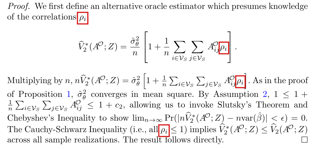
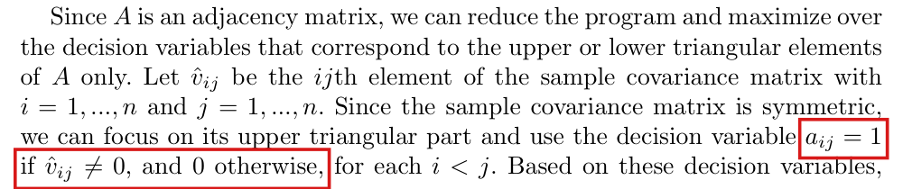
The correlations in the proof of Proposition 2 belong to pairs of units, ρij\rho_{ij}; they are printed four times with a single index, ρi\rho_i, which the paper does not define.

Proof of Proposition 2, p. 2246 (PDF p. 9): the sentence that defines the auxiliary estimator, its two displays, and “all ρi≤1\rho_i\le1”

See also under Formal statements (Lean): P011-T11, P011-T19, P011-T21, P011-T34

As printed

We first define an alternative oracle estimator which presumes knowledge of the correlations ρi\colorbox{#ffe58a}{$\rho_i$},

V^2∗(AO;Z)=σ^θ2n[1+1n∑i∈VS∑j∈VSAijOρi].\widehat V_2^*(A^{\mathcal O};Z)=\frac{\hat\sigma_\theta^2}{n}\left[1+\frac1n\sum_{i\in\mathcal V_S}\sum_{j\in\mathcal V_S}A^{\mathcal O}_{ij}\colorbox{#ffe58a}{$\displaystyle \rho_i$}\right].

Multiplying by nn, nV^2∗(AO;Z)=σ^θ2[1+1n∑i∈VS∑j∈VSAijOρi]n\widehat V_2^*(A^{\mathcal O};Z)=\hat\sigma_\theta^2\left[1+\frac1n\sum_{i\in\mathcal V_S}\sum_{j\in\mathcal V_S}A^{\mathcal O}_{ij}\colorbox{#ffe58a}{$\rho_i$}\right]. … The Cauchy-Schwarz Inequality (i.e., all ρi≤1\colorbox{#ffe58a}{$\rho_i$}\le1) implies V^2∗(AO;Z)≤V^2(AO;Z)\widehat V_2^*(A^{\mathcal O};Z)\le\widehat V_2(A^{\mathcal O};Z) across all sample realizations.

The problem

The symbol ρi\rho_i is not defined in the paper. The proof needs the correlation between θiYi\theta_iY_i and θjYj\theta_jY_j, which depends on the pair (i,j)(i,j): two neighbors of one vertex can have different correlations with it. The bound cov⁡(θiYi,θjYj)≤σθ2AijO\operatorname{cov}(\theta_iY_i,\theta_jY_j)\le\sigma_\theta^2A^{\mathcal O}_{ij} for distinct units, stated before (3.7), and the double sum over ii and jj show that the correlation of the pair is meant and that the index jj was dropped.

Evidence a derivation

I checked the page and derived the variance identity. Let Xi=θiYiX_i=\theta_iY_i, let σθ2>0\sigma_\theta^2>0 be the common variance, and let ρij=cov⁡(Xi,Xj)/σθ2\rho_{ij}=\operatorname{cov}(X_i,X_j)/\sigma_\theta^2. Since XiX_i and XjX_j are independent when i≠ji\ne j and AijO=0A^{\mathcal O}_{ij}=0, I have

nvar⁡(β^)=1n[∑i∈VSvar⁡(Xi)+∑i≠jcov⁡(Xi,Xj)]=σθ2[1+1n∑i∈VS∑j∈VSAijOρij].n\operatorname{var}(\hat\beta)=\frac1n\Bigl[\sum_{i\in\mathcal V_S}\operatorname{var}(X_i)+\sum_{i\ne j}\operatorname{cov}(X_i,X_j)\Bigr] =\sigma_\theta^2\Bigl[1+\frac1n\sum_{i\in\mathcal V_S}\sum_{j\in\mathcal V_S}A^{\mathcal O}_{ij}\rho_{ij}\Bigr].

This is the identity on which the auxiliary estimator is built. An example shows that no single index can stand for the pair. Let UU and VV be independent, each equal to 11 or −1-1 with probability 1/21/2, and let X1=UX_1=U, X2=3U/5+4V/5X_2=3U/5+4V/5 and X3=VX_3=V on the path with edges {1,2}\{1,2\} and {2,3}\{2,3\}. The three variances equal 11, the two correlations at vertex 2 are ρ12=3/5\rho_{12}=3/5 and ρ23=4/5\rho_{23}=4/5, and both sides of the identity equal 29/1529/15. An average of the ρij\rho_{ij} over the neighbors jj of ii would give the same double sum, but the paper defines no such quantity.

What survives

The inequality V^2∗(AO;Z)≤V^2(AO;Z)\widehat V_2^*(A^{\mathcal O};Z)\le\widehat V_2(A^{\mathcal O};Z) is unchanged, since ρij≤1\rho_{ij}\le1, AijO≥0A^{\mathcal O}_{ij}\ge0 and σ^θ2≥0\hat\sigma_\theta^2\ge0. The corrected index does not establish the consistency that the proof asserts for the auxiliary estimator (P011-E004).

Corrected

Let Xi=θiYiX_i=\theta_iY_i, and let σθ2=var⁡(Xi)\sigma_\theta^2=\operatorname{var}(X_i) be the common variance of Assumption 3. For i,j∈VSi,j\in\mathcal V_S define ρij=cov⁡(Xi,Xj)/σθ2\colorbox{#ffe58a}{$\rho_{ij}$}=\operatorname{cov}(X_i,X_j)/\sigma_\theta^2 if σθ2>0\sigma_\theta^2>0, and ρij=0\rho_{ij}=0 if σθ2=0\sigma_\theta^2=0. The auxiliary estimator is

V^2∗(AO;Z)=σ^θ2n[1+1n∑i∈VS∑j∈VSAijOρij],\widehat V_2^*(A^{\mathcal O};Z)=\frac{\hat\sigma_\theta^2}{n}\left[1+\frac1n\sum_{i\in\mathcal V_S}\sum_{j\in\mathcal V_S}A^{\mathcal O}_{ij}\colorbox{#ffe58a}{$\displaystyle \rho_{ij}$}\right],

with ρij\colorbox{#ffe58a}{$\rho_{ij}$} also in the display that follows “Multiplying by nn” and in “all ρij≤1\colorbox{#ffe58a}{$\rho_{ij}$}\le1”. Under Assumption 2, nvar⁡(β^)→c3>0n\operatorname{var}(\hat\beta)\to c_3>0, so σθ2>0\sigma_\theta^2>0 for all large nn.

Crop of the whole proof of Proposition 2. Four red boxes mark the symbol rho with subscript i: after the words 'of the correlations', at the end of the double sum in the displayed definition of V 2 star, at the end of the double sum in the line that begins 'Multiplying by n', and in the words 'all rho i less than or equal to 1'.
Proof of Proposition 2, p. 2246 (PDF p. 9). The four marked symbols are the correlations, each printed with the single index ii.

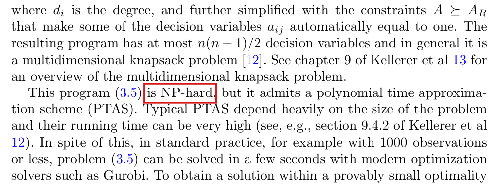
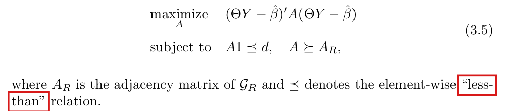
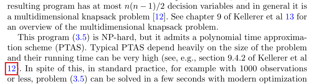
Program (3.5) is a maximum-weight degree-constrained subgraph problem, which is solved exactly in polynomial time by reduction to weighted matching; hence it is NP-hard only if P=NP\mathrm{P}=\mathrm{NP}.

P. 2245 (PDF p. 8), the two paragraphs after program (3.6)

Classification before my review (the classification when the audit was first completed, before I reviewed it): Error, Moderate (entry P011-E002).

See also under Formal statements (Lean): P011-T13, P011-T14, P011-T30

Revised: see the history of this entry.

As printed

“The resulting program has at most n(n−1)/2n(n-1)/2 decision variables and in general it is a multidimensional knapsack problem [12]. See chapter 9 of Kellerer et al 13 for an overview of the multidimensional knapsack problem.

This program (3.5) is NP-hard, but it admits a polynomial time approximation scheme (PTAS). Typical PTAS depend heavily on the size of the problem and their running time can be very high (see, e.g., section 9.4.2 of Kellerer et al 12).”

The problem

Programs (3.5) and (3.6) choose a set of edges on nn vertices so as to maximize a sum of edge weights. Each vertex has an upper bound on its degree, and the known edges must be included. Once the known edges are fixed and their incidences are subtracted from the degree bounds, this is a maximum-weight simple bb-matching problem. It reduces to ordinary maximum-weight matching on a graph of polynomial size, and matching is solved exactly in polynomial time. Program (3.8) is the case of unit weights. Program (3.5) is solvable in polynomial time; hence it is NP-hard only if P=NP\mathrm{P}=\mathrm{NP}. For its nontrivial threshold decision problem, NP-hardness is equivalent to P=NP\mathrm{P}=\mathrm{NP}, which is open. The error is the confident assertion of this unresolved classification. The program can be written as a multidimensional knapsack instance, in which each item uses one unit of exactly two resources. The hardness of the general knapsack problem does not transfer to this special case. The computational guidance should acknowledge the exact polynomial algorithm. General integer-programming solvers and certified relaxations remain valid options; no failure of their reported running times is established by this correction.

Evidence a derivation

I give an explicit reduction. Let bib_i be min⁡{di,n−1}\min\{d_i,n-1\} minus the number of known edges at ii, let the optional edges have integer weights WeW_e after scaling, and let M=1+max⁡({0}∪{∣We∣:e optional})M=1+\max(\{0\}\cup\{|W_e|:e\text{ optional}\}). For each vertex ii, I create bib_i slot vertices. For each optional edge e={i,j}e=\{i,j\}, I create two vertices joined by an edge of weight 4M4M, and I join them to every slot of ii and to every slot of jj, respectively, by edges of weight 2M+We2M+W_e. In a maximum-weight matching, the two vertices of each ee are matched either to each other or to slots at both ends. Together with the known edges, the optional edges whose vertices are matched to slots form an optimal solution of (3.6). The weight of the matching is 4Mq+2∑We4Mq+2\sum W_e, summed over those optional edges, where qq is the number of optional edges. The new graph has at most 2n(n−1)2n(n-1) vertices. I checked the reduction against exhaustive edge-set enumeration on 13,824 three-vertex inputs and on 96 rational inputs with four or five vertices.

The same check shows that the linear relaxation with degree constraints alone need not have an integral optimum.

Exact optima of the integer programs and of their linear relaxations in two examples with no known edge and every di=1d_i=1: six units with θiYi−β^=(1,1,1,−1,−1,−1)\theta_iY_i-\hat\beta=(1,1,1,-1,-1,-1), and three units.
QuantityInteger programLinear relaxation
Objective of (3.6), six units23
Objective of (3.5), six units46
V^1\widehat V_1 of (3.1) at the optimum, six units5/185/181/31/3
Objective of (3.8), three units23

The knapsack encoding remains valid. Where approximation ratios apply, an exact polynomial algorithm also supplies an approximation scheme. I have not tested the paper’s remark on the running time of Gurobi.

What survives

This computational correction leaves the formulations (3.5), (3.6) and (3.8), their optima, the maximal compatible estimators, the inequality between the maximal and the oracle estimators, and the upper bound from an optimal linear relaxation unchanged. No statistical result uses NP-hardness. General integer-programming solvers remain a valid way to solve the program. The comparisons of exact solvers with relaxations on p. 2248 and in Appendix B should mention the polynomial algorithm.

Corrected

“The resulting program has at most n(n−1)/2n(n-1)/2 decision variables. It can be encoded as a special multidimensional knapsack instance. Its degree-incidence structure makes it a maximum-weight simple bb-matching problem. After fixing the mandatory edges and subtracting their incidences from the degree bounds, it admits an exact polynomial-time solution by reduction to ordinary maximum-weight matching; hence it is NP-hard only if P=NP\mathrm{P}=\mathrm{NP}, which is open. Program (3.8) is its unit-weight case. General integer-programming solvers remain an implementation option; the linear relaxation with degree constraints alone can have fractional optima, and it still provides an upper bound when it is solved to optimality or comes with a certified bound.”

Crop of eleven lines of text. A red box marks the words 'is NP-hard' in the sentence 'This program (3.5) is NP-hard, but it admits a polynomial time approximation scheme (PTAS).' The lines above say that in general the program is a multidimensional knapsack problem.
P. 2245 (PDF p. 8), the paragraphs after program (3.6). The marked words classify program (3.5) as NP-hard.
History of this entry
  1. Classification before my review (the classification when the audit was first completed, before I reviewed it): Moderate error.
  2. Revised. The classification was lowered from a Moderate to a Minor error, and the wording was revised. How this came to light: review of the remaining Lean complexity statement showed that P011-E002 already covers the words “is NP-hard” on p. 2245. The exact polynomial-time route described in the finding makes NP-hardness of the nontrivial threshold decision problem equivalent to P=NP\mathrm{P}=\mathrm{NP}, which is open. Why it changed: the paper asserted this unresolved classification with unwarranted confidence, and little depends on it. The knapsack encoding, optimization formulations and their optima remain valid, as do the use of general integer-programming solvers and certified relaxation bounds; no statistical result uses NP-hardness. The reduction and the qualification about fractional LP optima are retained. The earlier Moderate rating is preserved as history. This revision was made at P. M. Aronow's decision and was written by the model session that runs the audit.
  3. Classification now: Minor error.

The decision variable aija_{ij} of program (3.6) is the indicator that the edge {i,j}\{i,j\} is selected, and not the indicator that v^ij≠0\hat v_{ij}\neq0.

Last paragraph of p. 2244 (PDF p. 7), the sentence that defines the decision variables of program (3.6)

See also under Formal statements (Lean): P011-T22, P011-T23, P011-T27

As printed

“Let v^ij\hat v_{ij} be the ijijth element of the sample covariance matrix with i=1,...,ni=1,...,n and j=1,...,nj=1,...,n. Since the sample covariance matrix is symmetric, we can focus on its upper triangular part and use the decision variable aij=1a_{ij}=1 if v^ij≠0\colorbox{#ffe58a}{$\hat v_{ij}\neq0$}, and 0 otherwise, for each i<ji<j.”

The problem

As printed, the data fix every aija_{ij}, and nothing is left to optimize. The values so fixed can violate the degree constraints of (3.6), and they can leave out a known edge whose coefficient is zero. Program (3.6), which is printed next, treats the aija_{ij} as free binary variables and v^ij\hat v_{ij} as their objective coefficients. The sentence also leaves the matrix with entries v^ij\hat v_{ij} undefined. By (3.5), its entries are the cross-products (θiYi−β^)(θjYj−β^)(\theta_iY_i-\hat\beta)(\theta_jY_j-\hat\beta).

Evidence an exact counterexample

I base this correction on an exact example. It has three units with θi=1\theta_i=1, centred outcomes (−2,1/2,3/2)(-2,1/2,3/2), degree bounds (1,1,1)(1,1,1) and no known edge. The products v^12\hat v_{12}, v^13\hat v_{13} and v^23\hat v_{23} are −1-1, −3-3 and 3/43/4. All are nonzero, and under the printed rule every vertex has degree 2. A maximizer of (3.6) selects the edge {2,3}\{2,3\} only. The package builds its objective from the outer product of the centred values and imposes the constraints on the degrees and on the known edges separately.

What survives

Program (3.6) and the package use the intended variable, and nothing depends on the sentence.

Corrected

“Let v^ij=(θiYi−β^)(θjYj−β^)\colorbox{#ffe58a}{$\hat v_{ij}=(\theta_iY_i-\hat\beta)(\theta_jY_j-\hat\beta)$} for i=1,...,ni=1,...,n and j=1,...,nj=1,...,n. Since this matrix is symmetric, we can focus on its upper triangular part and use the decision variable aij=1a_{ij}=1 if the edge {i,j}\{i,j\} is selected, and 0 otherwise, for each i<ji<j.”

Crop of the last six lines of the page. Red boxes mark 'a_ij = 1' at the end of one line and 'if v-hat_ij is not equal to 0, and 0 otherwise,' at the start of the next.
Last paragraph of p. 2244 (PDF p. 7). The marked clause defines the decision variable by a condition on the data.

“In both depgraph and depinf” should read “In both depgraph and depvar”: depinf is the package, and its two functions are depgraph and depvar.

Appendix B, p. 2250 (PDF p. 13), sentence beginning “In both depgraph and depinf”

As printed

In both depgraph and depinf, we give the option to find an exact solution to (3.5) and (3.8) via integer programming, or an approximate solution to the relaxations of (3.5) and (3.8) via linear programming.

The problem

The preceding sentence names the two functions of the package, depgraph and depvar. The second name in this sentence is the name of the package.

Evidence a check of the printed page

I checked the page and the package source. Both functions take the argument approximate, which selects the integer program or its relaxation, and depvar passes it to depgraph. The package defines no function named depinf.

What survives

Nothing else changes.

Corrected

“In both depgraph and depvar, we give the option to find an exact solution to (3.5) and (3.8) via integer programming, or an approximate solution to the relaxations of (3.5) and (3.8) via linear programming.”

Crop of nine lines of Appendix B. A red box marks the word 'depinf' in the sentence 'In both depgraph and depinf, we give the option to find an exact solution to (3.5) and (3.8)'. The sentence before it reads 'depinf includes two basic functions: depgraph, ... and depvar for calculating the variance estimates (3.1) and (3.7).'
Appendix B, p. 2250 (PDF p. 13). The marked name is that of the package; the preceding sentence names the two functions depgraph and depvar.

The function depgraph stops with an error when the matrix GR of known edges is supplied and contains no edge; in that case the row indices of the known-edge constraints must form an empty sequence.

R package depinf, named in Appendix B, p. 2250 (PDF p. 13): R/depgraph.r, lines 27–34, with lines 73 and 82. The code is not printed in the article.

As printed

Lines 30 and 33 of R/depgraph.r, inside the block if (!is.null(GR)):

rows_GR = (row_count+1):(row_count+length(cols_GR))

row_count = max(rows_GR)

The problem

The article allows a recruitment graph with no known edge: on p. 2248 the constraint A⪰ARA\succeq A_R becomes A⪰0A\succeq 0 and is superfluous. A matrix GR of zeros encodes this case, and it should produce the same program as GR = NULL. In the code, cols_GR is then empty, and in R the expression (row_count+1):(row_count+0) is a descending sequence of length two and not an empty sequence. The right-hand side and the vector of constraint directions (lines 73 and 82) receive two entries that correspond to no row of the constraint matrix, and the solver rejects the program.

Evidence an exact counterexample

I base this correction on an exact example, run with the package and the GLPK solver. Let v be the 3×33\times3 matrix of ones, let d=(1,1,1)d=(1,1,1), and let GR be the 3×33\times3 matrix of zeros. Then the vector rows_GR is 4:3. The constraint matrix has three rows, and the right-hand side and the directions have length five. The solver interface stops with the message Arguments 'mat', 'dir', and/or 'rhs' not conformable. The same failure occurs with the scalar d = 1 (one row against three entries), for the integer program and for the linear program, and in both branches of depvar that call depgraph. With the two corrected lines, a matrix of zeros and GR = NULL produce the same program and the same answer in these tests, and the tested calls with known edges are unchanged.

What survives

No wrong number is produced, because the call stops. The equivalent call GR = NULL works. The calls of the vignette pass NULL or a matrix with edges (97 known edges in the example data and 468 in the application), and they do not take this path. The programs, estimators and proofs of the article do not depend on this code. The CPLEX and Gurobi branches receive the same program, and they were not run.

Corrected

rows_GR = row_count + seq_along(cols_GR)

row_count = row_count + length(cols_GR)

Listing in monospaced type with line numbers. A red box marks line 30, 'rows_GR = (row_count+1):(row_count+length(cols_GR))', and a second red box marks line 33, 'row_count = max(rows_GR)'. Lines 73 and 82 below them build the vectors bvec and sense with length(rows_GR) further entries.
Package depinf, file R/depgraph.r, lines 27–34, 72–74 and 81–83, typeset from the file with line numbers added. The two marked lines build the row indices of the known-edge constraints.

For case = "homoskedastic" with GR = NULL, the function depvar returns the estimator (3.7) at an optimized graph, not the closed form (3.9) that its help page states, and the vignette labels this output V^2′\widehat V_2'.

Package depinf: man/depvar.Rd, line 24; R/depvar.r, lines 39–53; vignettes/replication.Rmd, lines 114–119. In the article: equation (3.9), p. 2247 (PDF p. 10); Appendix B, p. 2250 (PDF p. 13)

As printed

Help page of depvar (man/depvar.Rd, line 24, with the code markup of the source shown as typewriter text): “If case = homoskedastic and GR is not NULL, then (7) in section 3.2 of the same paper is calculated. Finally, if case = homoskedastic and GR is NULL, (9) is calculated.”

R/depvar.r, lines 39 and 42, and lines 51 and 52:

else if (case=="homoskedastic") {

out = depgraph(v, d, GR, solver, approximate)

else if (case=="homoskedastic") {

V_hat = V2(A_max, x)

vignettes/replication.Rmd, lines 114 and 115; lines 116 to 118 repeat the call for coefficients 2 to 4, and line 119 collects the four values as col7:

# V2'

d1 = sqrt(depvar(Y, Theta[1, ]*n, d, NULL, case = "homoskedastic")$V_hat)

The problem

The help page promises the closed form (3.9), which depends on the degrees only. The code does not compute it in this call. In the comparisons below, I use the package’s variance divisor n−1n-1 for both formulas; its difference from the paper’s divisor nn is addressed in P011-E015. For case = "homoskedastic" it always calls depgraph, which solves program (3.8), by default its linear relaxation, with no known edges when GR is NULL. It then returns (3.7) at that solution. Since each row sum of a feasible matrix is at most min⁡{di,n−1}\min\{d_i,n-1\}, the returned value is at most (3.9). When the sample variance is positive, it is strictly smaller unless every row attains its bound. The vignette labels the output of this call V2'. The four standard errors in its column col7 are values of (3.7) under the label of (3.9). Appendix B of the article describes depvar correctly, as “calculating the variance estimates (3.1) and (3.7)”.

Evidence an exact counterexample

I used an exact example and a recalculation. Let y=(0,1,2)y=(0,1,2), θ=(1,1,1)\theta=(1,1,1) and d=(2,0,0)d=(2,0,0), with GR = NULL. The degree bounds of vertices 2 and 3 exclude every edge, and the zero matrix is the only feasible point of (3.8) and of its relaxation. The package’s sample variance is 11. The returned value is then 1/31/3, while the closed form is (1/3)(1+2/3)=5/9(1/3)(1+2/3)=5/9. The unmodified function returns 1/31/3 with approximate = 1 and with approximate = 0. With the paper’s divisor nn in place of the package’s divisor n−1n-1 (P011-E015), the two values are 2/92/9 and 10/2710/27. On the vignette’s data, with n=522n=522, the truncated degrees sum to 85618561 and the relaxed program without known edges attains 85608560. The resulting standard errors agree with the printed col7 and not with the closed form, which the vignette’s sensitivity table computes directly.

Standard errors for the vignette’s four coefficients: its column col7, and the two estimators recalculated using the package’s variance divisor n−1n-1.
Coefficientcol7 as printed(3.7) at the optimized graphClosed form (3.9)
intercept0.439152510.439152510.43917668
hcv0.191998570.191998570.19200914
age0.014745040.014745040.01474585
sex0.271736660.271736660.27175162
What survives

The two underlying formulas are bounds of the paper, and (3.7) at the optimized graph is no larger than (3.9) when the same variance divisor is used. No loss of conservativeness is shown, and no number in the article is affected. Equations (3.7) and (3.9), Lemma 1 and Appendix B are unchanged. What changes is the description of this call in the help page and the label of col7 in the vignette, or else the value that the call returns.

Corrected

To honor the help page’s choice of estimator while retaining the package’s variance divisor n−1n-1 (P011-E015), the code changes. For case = "homoskedastic" and GR = NULL, before any graph program is solved, set x = y*theta and n = length(x) and return, for a vector d, var(x)/n * (1 + sum(pmin(d, n-1))/n), with A_max = NULL, obj_val = NA_real_ and time = 0. For a scalar d, which the help page defines as the total number of nonzero off-diagonal entries of AA, return var(x)/n * (1 + min(d, n*(n-1))/n). The optimized estimator is kept when GR is not NULL. The four values of col7 in the vignette then become 0.439176680.43917668, 0.192009140.19200914, 0.014745850.01474585 and 0.271751620.27175162.

A smaller correction keeps the code and every number, and changes the documentation. Help page: “Finally, if case = homoskedastic and GR is NULL, (7) is calculated at the solution of (8) with no known dependencies (by default, of its linear relaxation).” Vignette, line 114: # V2, no known dependencies. The closed form (3.9) is then obtained directly, as in the sensitivity analysis of the vignette.

Crop of equation (3.9), which defines V 2 prime of Z as sigma hat theta squared over n, times 1 plus the average of the truncated degrees d i prime, followed by Lemma 1. Red boxes mark the sentence 'The estimator (3.9) does not depend on any particular compatible adjacency matrix.'
Equation (3.9), p. 2247 (PDF p. 10): the closed form that the help page promises for this call. The marked sentence is correct; the defect is in the package, whose output for this call does depend on an adjacency matrix.
Listing of line 24 of the file depvar.Rd in typewriter type, on five rows. Red boxes mark the last sentence: 'Finally, if code case = homoskedastic and code GR is code NULL, (9) is calculated.'
Help page of depvar, source file man/depvar.Rd, line 24, typeset from the package with the line number added and the long line continued on four further rows. The marked sentence says that (9) is calculated when GR is NULL.
Listing of lines 39 to 53 of the file depvar.r. Red boxes mark line 42, 'out = depgraph(v, d, GR, solver, approximate)', and line 52, 'V_hat = V2(A_max, x)'. No line of the listing treats GR = NULL separately.
R/depvar.r, lines 39–53, typeset from the package with line numbers added. The marked lines call depgraph for every homoskedastic case and evaluate V2 at the graph it returns.
Listing of lines 114 to 119 of the file replication.Rmd. A red box marks the comment '# V2 prime' on line 114. Lines 115 to 118 assign d1 to d4 as the square root of the V_hat returned by depvar with arguments NULL and case = "homoskedastic", and line 119 collects them as col7.
vignettes/replication.Rmd, lines 114–119, typeset from the package with line numbers added. The marked comment labels the four calls below it as V^2′\widehat V_2'.

The option case = "homoskedastic, worst" of depvar, which is the only route to the closed form (3.9), stops with an error because three of the fields that it returns are never assigned.

R package depinf, named in Appendix B, p. 2250 (PDF p. 13): R/depvar.r, lines 23–29 and 54–58. The code is not printed in the article, and the option is not listed in the help page man/depvar.Rd.

As printed

Lines 54–58 of R/depvar.r:

else if (case=="homoskedastic, worst") {

V_hat = V2p(d, x)

}

return(list(V_hat = V_hat, A_max = A_max, obj_val = obj_val, time = time))

Line 26, in the helper V2p: n = length(d)

The problem

The branch assigns V_hat only. The return statement on line 58 also evaluates A_max, obj_val and time, which are assigned only in the two branches that call depgraph. In a clean R session the call stops with object 'A_max' not found. A second defect lies on the same path. The helper V2p takes the sample size from the length of d. This is the number of observations when d is a vector of degrees, which is the case of the article. For a scalar d it is 1.

Evidence an exact counterexample

I base this correction on a run of the package code and an exact enumeration. With outcomes (0,1,2)(0,1,2), θ=(1,1,1)\theta=(1,1,1), no known edge, and d=(2,0,0)d=(2,0,0) or d=(2,2,2)d=(2,2,2), the call stops at the return statement, and no solver is involved. The helper computes 5/95/9 and 11 for these two inputs. If only the return statement is repaired, then for the scalar d=0d=0 the call returns 11, where the value with no edge is 1/31/3. Replacing length(d) by length(x) does not handle a scalar either. The help page defines a scalar d as a bound on the total number of nonzero off-diagonal entries. With this meaning, d=6d=6 allows the complete graph on three vertices, for which the formula of the helper equals 11, and the helper with length(x) returns 5/95/9. An enumeration of the eight graphs on three vertices confirms these values.

What survives

Equation (3.9), Lemma 1 and Corollaries 2 and 4 are not affected, because the defect is in the software only. No wrong number is returned, because the call stops. Nothing in the article, the help pages or the vignette calls this option. The vignette obtains its values labelled V^2′\widehat V_2' from the documented case "homoskedastic" (see P011-E012), and its sensitivity analysis computes the closed form directly.

Corrected

On the branch case=="homoskedastic, worst", require length(d) == length(x) and assign the three fields:

V_hat = V2p(d, x)

A_max = NULL; obj_val = NA_real_; time = 0

In the helper V2p, take the sample size from the observations: n = length(x). The option and the placeholder values should be documented in the help page. If a scalar d is also accepted with its documented meaning, a bound DD on the total number of nonzero off-diagonal entries, use min⁡{D,n(n−1)}\min\{D,n(n-1)\} as an upper bound on the sum of the degrees in the closed form. A common bound for every vertex is a different input, and it must be expanded to a vector of length nn.

Listing in monospaced type with line numbers. Red boxes mark 'n = length(d)' on line 26, 'V_hat = V2p(d, x)' on line 55, and 'A_max = A_max, obj_val = obj_val, time = time' inside the return statement on line 58.
Package depinf, file R/depvar.r, lines 23–29 and 48–58, typeset from the file with line numbers added. The branch on line 55 assigns V_hat only, and line 58 returns three further objects.

The function depgraph uses the solver’s output without checking that the solve succeeded: after a failed GLPK solve it returns a graph and an objective value as if they were optimal.

Appendix B, p. 2250 (PDF p. 13). Package depinf: R/depgraph.r, lines 156–183 (GLPK), 116–155 (Gurobi) and 92–115 (CPLEX)

As printed

Appendix B, p. 2250: “In order to solve (3.5) and (3.8), depgraph can use three different optimization solvers: CPLEX, GLPK and Gurobi. By default, depgraph uses GLPK, …”

R/depgraph.r, lines 165, 173 to 175, 178, 179 and 182 (line 165 is broken here to fit the page):

out = Rglpk_solve_LP(cvec, Amat, dir, bvec, bounds = bound,types = var_type, max = TRUE)group_1 = i_ind[out$solution!=0]group_2 = j_ind[out$solution!=0]approx_sol = out$solutiongroup_1 = i_ind[out$solution==1]group_2 = j_ind[out$solution==1]obj_val = out$optimum\begin{aligned} &\texttt{out = Rglpk\_solve\_LP(cvec, Amat, dir, bvec, bounds = bound,}\\ &\qquad\texttt{types = var\_type, max = TRUE)}\\ &\texttt{group\_1 = i\_ind[}\colorbox{#ffe58a}{$\displaystyle \texttt{out\$solution}$}\texttt{!=0]}\\ &\texttt{group\_2 = j\_ind[}\colorbox{#ffe58a}{$\displaystyle \texttt{out\$solution}$}\texttt{!=0]}\\ &\texttt{approx\_sol = }\colorbox{#ffe58a}{$\displaystyle \texttt{out\$solution}$}\\ &\texttt{group\_1 = i\_ind[}\colorbox{#ffe58a}{$\displaystyle \texttt{out\$solution}$}\texttt{==1]}\\ &\texttt{group\_2 = j\_ind[}\colorbox{#ffe58a}{$\displaystyle \texttt{out\$solution}$}\texttt{==1]}\\ &\texttt{obj\_val = }\colorbox{#ffe58a}{$\displaystyle \texttt{out\$optimum}$} \end{aligned}
The problem

After the call to the solver, depgraph reads the solution vector and the objective value and returns them as the maximizing graph A_max and the optimum obj_val. None of its three branches tests the status that the solver reports. When a solve fails, the result is returned as an ordinary one, with no error and no warning, and depvar computes a variance estimate from it. The Gurobi branch sets a time limit of 12 hours and reads the returned solution and objective in the same way. If the limit were reached, a returned incumbent would be only a lower bound on the maximum, and it need not dominate the oracle estimator.

Evidence an exact counterexample

I used the saved output of a GLPK run of the package and exact arithmetic. Let n=3n=3 and d=(0,0,0)d=(0,0,0), let GR contain the single edge {1,2}\{1,2\}, and let every objective coefficient equal 11. Since the constraints a12=1a_{12}=1 and a12+a13≤0a_{12}+a_{13}\le0 contradict each other, the integer program and its relaxation are infeasible. GLPK (Rglpk 0.6.5.1, GLPK 5.0) returns status 11, the solution (0,0,0)(0,0,0) and the objective 00 in both modes. The unmodified depgraph then returns the zero matrix as A_max and obj_val = 0, although the known edge requires A12=1A_{12}=1. With y=(1,1,−2)y=(1,1,-2) and θ=(1,1,1)\theta=(1,1,1), depvar returns V_hat = 1 in each of the four combinations of case and mode. These inputs lie outside the paper’s framework, in which AOA^{\mathcal O} is compatible with the data and the feasible set is not empty.

For the Gurobi branch the evidence is a reading of the code and an exact example of what an incumbent can do. For n=4n=4, y=(1,1,−1,−1)y=(1,1,-1,-1), θi=1\theta_i=1 and d=(1,1,1,1)d=(1,1,1,1), the zero graph is feasible with objective 00 and the maximum is 22. Equation (3.1) gives 1/41/4 at the zero graph and 1/21/2 at the maximizer. Neither Gurobi nor CPLEX was run. No failed or interrupted solve was observed on data that satisfy the paper’s assumptions.

What survives

The results of the paper concern the maximal compatible estimator or an upper bound on it, and they are not affected. Solves that succeed, the bound from a solved relaxation and the closed form (3.9) are unaffected. No number in the article is involved, and no value of the vignette is shown to come from a failed solve. The vignette raises each degree to at least the number of known edges at the vertex, so the contradictory input above cannot arise there. What changes is that a failed solve must stop with an error.
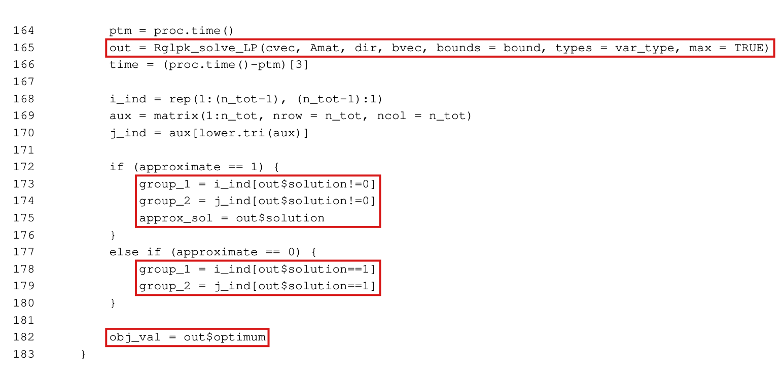
Corrected

In the GLPK branch, immediately after line 165 and before out$solution or out$optimum is used, insert the following statement (broken here over three lines).

if (!identical(out$status, 0L))stop(sprintf("GLPK did not find an optimal solution (status %s)",out$status))\begin{aligned} &\colorbox{#ffe58a}{$\displaystyle \texttt{if (!identical(out\$status, 0L))}$}\\ &\qquad\colorbox{#ffe58a}{$\displaystyle \texttt{stop(sprintf("GLPK did not find an optimal solution (status \%s)",}$}\\ &\qquad\qquad\colorbox{#ffe58a}{$\displaystyle \texttt{out\$status))}$} \end{aligned}

Under the default convention of Rglpk_solve_LP, status 00 means that an optimal solution was found. With this statement in place, both infeasible calls above stop with the message “GLPK did not find an optimal solution (status 1)”, and a feasible control with d=(1,1,0)d=(1,1,0) and the same known edge returns status 00 and the same graph and objective as before. This correction does not cover the CPLEX and Gurobi branches, each of which needs its own test of the termination status. If an interrupted maximization is to be used for inference, the variance bound for (3.1) should be computed from a certified upper bound UU on the objective of (3.6), as (nσ^θ2+2U)/n2(n\hat\sigma_\theta^2+2U)/n^2, and not from the incumbent.

Crop of five lines of Appendix B. A red box marks the words 'By default, depgraph uses GLPK,'. The line before it reads 'In order to solve (3.5) and (3.8), depgraph can use three different optimization solvers: CPLEX, GLPK and Gurobi.'
Appendix B, p. 2250 (PDF p. 13). The marked sentence names GLPK as the default solver; the defect is in the GLPK branch of depgraph.
Listing of lines 164 to 183 of the file depgraph.r. Red boxes mark line 165, 'out = Rglpk_solve_LP(cvec, Amat, dir, bvec, bounds = bound, types = var_type, max = TRUE)'; lines 173 to 175, which read out$solution; lines 178 and 179, which read out$solution; and line 182, 'obj_val = out$optimum'. No line of the listing mentions out$status.
R/depgraph.r, lines 164–183, typeset from the package with line numbers added. The marked lines are the call to the solver and every later use of its output; none tests the status of the solve.

The package’s variance helpers use divisor n−1n-1 where the paper defines the sample variance with divisor nn, so their values can exceed (3.1), (3.7) and (3.9).

Section 3.1, p. 2242 (PDF p. 5), the definition of σ^θ2\hat\sigma_\theta^2 before (3.1); Appendix B, p. 2250 (PDF p. 13); R package depinf, R/depvar.r, lines 11, 19 and 27

See also under Formal statements (Lean): P011-T25, P011-T26, P011-T35

As printed

P. 2242: “Define the plug-in sample variance σ^θ2=n−1∑i∈VS(θiYi−β^)2\hat\sigma_\theta^2=n^{-1}\sum_{i\in\mathcal V_S}(\theta_iY_i-\hat\beta)^2”. Appendix B, p. 2250: “depvar for calculating the variance estimates (3.1) and (3.7)”.

R/depvar.r, line 11: V1_hat = as.numeric( var(x)/n + (t(x-mx) %*% A %*% (x-mx))/(n^2\texttt{n\textasciicircum 2}) )

Line 19: V2_hat = as.numeric( var(x)/n * (1 + sum(A)/n) )

Line 27: V2_hat = as.numeric( var(x)/n * (1 + sum(pmin(d, n-1))/n) )

The problem

For complete data with n>1n>1 and a degree vector of length nn, the function var of R divides by n−1n-1. Let xi=θiYix_i=\theta_iY_i and S=∑i(xi−xˉ)2S=\sum_i(x_i-\bar x)^2. At a fixed AA, the value of V^1\widehat V_1 in the package exceeds (3.1) by S/[n2(n−1)]S/[n^2(n-1)], and the cross-product term is the same. The values of V^2\widehat V_2 and V^2′\widehat V_2' in the package equal (3.7) and (3.9) multiplied by n/(n−1)n/(n-1).

Evidence an exact counterexample

I base this correction on this derivation and an exact example, run with the package. For x=(0,1,2)x=(0,1,2), θ=(1,1,1)\theta=(1,1,1), d=(0,0,0)d=(0,0,0) and A=0A=0, the value of (3.1) is 2/92/9 and the package returns 1/31/3.

What survives

The difference is upward. Under Assumption 2 the V^1\widehat V_1 difference tends to zero after multiplication by nn; for V^2\widehat V_2 and V^2′\widehat V_2', the factor n/(n−1)n/(n-1) tends to one and preserves any otherwise valid asymptotic conservativeness guarantee. The maximizing graphs are the same, since σ^θ2\hat\sigma_\theta^2 does not depend on AA. No statement of the paper changes, and the article contains no numerical simulation or application table. I have not recomputed the standard errors of the vignette. The change of divisor does not repair P011-E001.

Corrected

In the helpers V1, V2 and V2p of R/depvar.r, replace each var(x) by mean((x-mean(x))^2)\colorbox{#ffe58a}{$\texttt{mean((x-mean(x))\textasciicircum 2)}$}. At a fixed AA, the value of V^1\widehat V_1 then decreases by S/[n2(n−1)]S/[n^2(n-1)], and the values of V^2\widehat V_2 and V^2′\widehat V_2' are multiplied by (n−1)/n(n-1)/n. Make the same replacement in the standalone closed-form calculation in inst/doc/replication.R, line 126.

Crop of the first three lines of Section 3.1 and display (3.1). A red box marks the factor n to the power minus 1 in 'plug-in sample variance sigma-hat-theta squared = n^-1 times the sum over i in V_S of (theta_i Y_i - beta-hat) squared'.
Section 3.1, p. 2242 (PDF p. 5). The marked factor is the divisor nn in the definition of the plug-in sample variance, which enters (3.1).
Listing in monospaced type with line numbers, showing the helper functions V1, V2 and V2p. Red boxes mark the call 'var(x)' at the start of the expression assigned to V1_hat on line 11, of the expression 'var(x)/n * (1 + sum(A)/n)' on line 19, and of the expression 'var(x)/n * (1 + sum(pmin(d, n-1))/n)' on line 27.
Package depinf, file R/depvar.r, lines 7–29, typeset from the file with line numbers added. Each of the three helpers calls var(x), which divides by n−1n-1.
Crop of the first six lines of Appendix B. A red box marks the clause 'depvar for calculating the variance estimates (3.1) and (3.7).'
Appendix B, p. 2250 (PDF p. 13). The marked clause says that depvar calculates the variance estimates (3.1) and (3.7).

In display (3.3) the weights θj\theta_j and θi\theta_i are each missing once, and the opening bracket of the subtracted product of expectations is misplaced.

Display (3.3), p. 2243 (PDF p. 6): the second line, the line that begins “+ E[β^4]+\,\mathrm{E}[\hat\beta^4]”, and the line after it

See also under Formal statements (Lean): P011-T17, P011-T18

As printed
ξijkl=cov⁡((θiYi−β^)(θjYj−β^),(θkYk−β^)(θlYl−β^))=E[(θiYi−β^)(Yj−β^)(θkYk−β^)(θlYl−β^)]−E[(θiYi−β^)(θjYj−β^)]E[(θkYk−β^)(θlYl−β^)]=⋯+E[β^4]−θiθjθkθl[E[YiYj]E[YkYl]−θiθjθkE[YiYj]E[Ykβ^]−θiθjθlE[YiYj]E[Ylβ^]+θiθjE[YiYj]E[β^2]−θkθlE[Yiβ^]E[YkYl]+⋯+E[β^2]E[β^2]]\begin{aligned} \xi_{ijkl}&=\operatorname{cov}\bigl((\theta_iY_i-\hat\beta)(\theta_jY_j-\hat\beta),(\theta_kY_k-\hat\beta)(\theta_lY_l-\hat\beta)\bigr)\\ &=\mathrm{E}\bigl[(\theta_iY_i-\hat\beta)\colorbox{#ffe58a}{$\displaystyle (Y_j-\hat\beta)$}(\theta_kY_k-\hat\beta)(\theta_lY_l-\hat\beta)\bigr]\\ &\quad-\mathrm{E}\bigl[(\theta_iY_i-\hat\beta)(\theta_jY_j-\hat\beta)\bigr]\mathrm{E}\bigl[(\theta_kY_k-\hat\beta)(\theta_lY_l-\hat\beta)\bigr]\\ &=\cdots+\mathrm{E}[\hat\beta^4]-\theta_i\theta_j\theta_k\theta_l\colorbox{#ffe58a}{$\displaystyle \bigl[$}\mathrm{E}[Y_iY_j]\mathrm{E}[Y_kY_l]-\theta_i\theta_j\theta_k\mathrm{E}[Y_iY_j]\mathrm{E}[Y_k\hat\beta]\\ &\quad-\theta_i\theta_j\theta_l\mathrm{E}[Y_iY_j]\mathrm{E}[Y_l\hat\beta]+\theta_i\theta_j\mathrm{E}[Y_iY_j]\mathrm{E}[\hat\beta^2]-\colorbox{#ffe58a}{$\displaystyle \theta_k\theta_l$}\mathrm{E}[Y_i\hat\beta]\mathrm{E}[Y_kY_l]+\cdots+\mathrm{E}[\hat\beta^2]\mathrm{E}[\hat\beta^2]\bigr] \end{aligned}
The problem

The definition printed above the display is ξijkl=cov⁡((θiYi−β^)(θjYj−β^),(θkYk−β^)(θlYl−β^))\xi_{ijkl}=\operatorname{cov}\bigl((\theta_iY_i-\hat\beta)(\theta_jY_j-\hat\beta),(\theta_kY_k-\hat\beta)(\theta_lY_l-\hat\beta)\bigr). The first expectation is taken of a product whose second factor is θjYj−β^\theta_jY_j-\hat\beta. In the expansion of the subtracted product of two expectations, the first of the sixteen terms is θiθjθkθlE[YiYj]E[YkYl]\theta_i\theta_j\theta_k\theta_l\mathrm{E}[Y_iY_j]\mathrm{E}[Y_kY_l], and the bracket must open before it. As printed, the product θiθjθkθl\theta_i\theta_j\theta_k\theta_l multiplies all sixteen terms. The term in E[Yiβ^]E[YkYl]\mathrm{E}[Y_i\hat\beta]\mathrm{E}[Y_kY_l] carries θiθkθl\theta_i\theta_k\theta_l.

Evidence a derivation

The corrected display follows from the identity cov⁡(U,V)=E[UV]−E[U]E[V]\operatorname{cov}(U,V)=\mathrm{E}[UV]-\mathrm{E}[U]\mathrm{E}[V] and a termwise expansion. For a numerical check, let Y=(1,1,1,1)Y=(1,1,1,1) and θ=(2,3,4,5)\theta=(2,3,4,5) be constants. In this case β^=7/2\hat\beta=7/2 and the covariance is 0. The unexpanded expression as printed equals 9/49/4, the expansion as printed equals 93009/1693009/16, and the corrected display equals 0.

What survives

The sixteen terms of the first expectation are correct as printed. The covariance terms of display (3.4), which the proof uses, agree with the corrected expansion. The other error in the proof of Proposition 1 is separate (see P011-E001).

Corrected

The identity in weighted variables requires the displayed weighted moments to exist. The raw-outcome expansion below is read where its individual mixed moments exist. Assumption 2 bounds Xi=θiYiX_i=\theta_iY_i; it does not by itself ensure raw moments for coordinates with θi=0\theta_i=0. Let Xi=θiYiX_i=\theta_iY_i. Then

ξijkl=E[(Xi−β^)(Xj−β^)(Xk−β^)(Xl−β^)]−QijQkl,Qij=θiθjE[YiYj]−θiE[Yiβ^]−θjE[Yjβ^]+E[β^2].\begin{aligned} \xi_{ijkl}&=\mathrm{E}\bigl[(X_i-\hat\beta)\colorbox{#ffe58a}{$\displaystyle (X_j-\hat\beta)$}(X_k-\hat\beta)(X_l-\hat\beta)\bigr]-Q_{ij}Q_{kl},\\ Q_{ij}&=\theta_i\theta_j\mathrm{E}[Y_iY_j]-\theta_i\mathrm{E}[Y_i\hat\beta]-\theta_j\mathrm{E}[Y_j\hat\beta]+\mathrm{E}[\hat\beta^2]. \end{aligned}

The sixteen terms of the first expectation are those printed, and the sixteen terms of QijQklQ_{ij}Q_{kl} are those printed inside the bracket, with three changes to the printed form.

  1. The second factor of the first expectation is (θjYj−β^)(\colorbox{#ffe58a}{$\theta_j$}Y_j-\hat\beta).
  2. The subtracted block begins −[θiθjθkθlE[YiYj]E[YkYl]−⋯-\colorbox{#ffe58a}{$\bigl[$}\theta_i\theta_j\theta_k\theta_l\mathrm{E}[Y_iY_j]\mathrm{E}[Y_kY_l]-\cdots.
  3. The fifth term of the block is −θiθkθlE[Yiβ^]E[YkYl]-\colorbox{#ffe58a}{$\theta_i$}\theta_k\theta_l\mathrm{E}[Y_i\hat\beta]\mathrm{E}[Y_kY_l].
Crop of the whole of display (3.3), thirteen lines. Red boxes mark the factor '(Y_j - beta-hat)' in the second line, the product 'theta_i theta_j theta_k theta_l' followed by an opening bracket in the line that begins '+ E[beta-hat^4]', and the term '- theta_k theta_l E[Y_i beta-hat] E[Y_k Y_l]' at the end of the next line.
Display (3.3), p. 2243 (PDF p. 6). The three marked places are the factor without θj\theta_j, the prefactor printed before the opening bracket, and the term without θi\theta_i.

Five slips of notation: θ\theta is missing from two restatements of the observed data ZZ, “less-than” should read “less-than-or-equal-to”, Assumption 3 should quantify over VS\mathcal V_S, and the edge set ES\mathcal E_S is printed once with a roman E.

Assumption 2, p. 2242 (PDF p. 5); the sentence after (3.5), p. 2244 (PDF p. 7); Assumption 3 and the last paragraph of p. 2246 (PDF p. 9); Discussion, p. 2248 (PDF p. 11)

See also under Formal statements (Lean): P011-T24, P011-T36

As printed
  1. P. 2242, Assumption 2: “observed data Z=(GR,Y,d)\colorbox{#ffe58a}{$Z=(\mathcal G_R,Y,d)$}”.
  2. P. 2248, Discussion: “Assumption 1, which states that we observe Z=(Y,d,GR)\colorbox{#ffe58a}{$Z=(Y,d,\mathcal G_R)$}”.
  3. P. 2244: “⪯\preceq denotes the element-wise “less-than” relation”.
  4. P. 2246, Assumption 3: “var⁡(θiYi)=var⁡(θjYj), ∀i,j∈V\operatorname{var}(\theta_iY_i)=\operatorname{var}(\theta_jY_j),\ \forall i,j\in\colorbox{#ffe58a}{$\mathcal V$}”.
  5. P. 2246, last paragraph: “the maximum number of edges that can be in ES\colorbox{#ffe58a}{$\mathrm{E}_S$}”.
The problem

By Assumption 1 and the sentence after it (p. 2240), I have Z=(Y,d,θ,GR)Z=(Y,d,\theta,\mathcal G_R), and the coefficients θ\theta are observed. The constraints A1⪯dA\mathbf{1}\preceq d and A⪰ARA\succeq A_R are not strict, since Definition 4 requires ∑jAij≤di\sum_jA_{ij}\le d_i. Section 2 defines θ1,…,θn\theta_1,\ldots,\theta_n for the observed vertices only, and NN may exceed nn, so that θiYi\theta_iY_i is undefined for i∈V∖VSi\in\mathcal V\setminus\mathcal V_S. Every sum in (3.7), (3.8) and (3.9) and in the proof of Lemma 1 runs over VS\mathcal V_S. Definition 2 writes the edge set of GS\mathcal G_S as ES\mathcal E_S, and the roman E denotes expectation elsewhere.

Evidence a check of the printed page

I base these corrections on a check of the pages against the definitions of Section 2. Four further points of notation were examined and are not defects: the two definitions of Θ\Theta (pp. 2241 and 2244) have separate scopes, the upper limit nn on the sums of p. 2241 is redundant, the scalar β^\hat\beta in ΘY−β^\Theta Y-\hat\beta is subtracted from each entry, and AmA^m in Lemma 1 is the maximizer for V^2\widehat V_2.

What survives

No result changes. Each item is corrected from the definitions nearby.

Corrected
  1. Assumption 2: “observed data Z=(Y,d,θ,GR)Z=(\colorbox{#ffe58a}{$Y,d,\theta,\mathcal G_R$})”.
  2. Discussion: “Assumption 1, which states that we observe Z=(Y,d,θ,GR)Z=(\colorbox{#ffe58a}{$Y,d,\theta,\mathcal G_R$})”.
  3. “⪯\preceq denotes the element-wise “less-than-or-equal-to” relation”.
  4. Assumption 3: “var⁡(θiYi)=var⁡(θjYj), ∀i,j∈VS\operatorname{var}(\theta_iY_i)=\operatorname{var}(\theta_jY_j),\ \forall i,j\in\colorbox{#ffe58a}{$\mathcal V_S$}”.
  5. “the maximum number of edges that can be in ES\colorbox{#ffe58a}{$\mathcal E_S$}”.
Crop of Assumption 2 (Asymptotic scaling), eight lines. A red box marks 'Z = (G_R, Y, d)' in the second line, 'graphs G and observed data Z = (G_R, Y, d), where G_R = (V_S, E_R)'.
Assumption 2, p. 2242 (PDF p. 5). The marked list of the observed data omits θ\theta.
Crop of display (3.5), 'maximize (Theta Y - beta-hat)' A (Theta Y - beta-hat) subject to A1 precedes-or-equals d, A succeeds-or-equals A_R', and the two lines after it. Red boxes mark the hyphenated word 'less-than', in quotation marks, which is split over two lines.
Program (3.5) and the sentence after it, p. 2244 (PDF p. 7). The marked word describes the relation ⪯\preceq of the constraint A1⪯dA\mathbf{1}\preceq d.
Crop of the line 'Assumption 3 (Homoskedasticity). var(theta_i Y_i) = var(theta_j Y_j), for all i, j in V.' and the two lines after it. A red box marks the calligraphic V at the end of the assumption.
Assumption 3, p. 2246 (PDF p. 9). The marked set is the full vertex set V\mathcal V.
Crop of three lines. A red box marks 'E_S', with an upright E, in 'of edges that can be in E_S. For i in V_S, let d-prime_i = min{d_i, n - 1} be the degree of'.
Last paragraph of p. 2246 (PDF p. 9). The marked symbol is the edge set, printed with a roman E.
Crop of the first seven lines of the Discussion. Red boxes mark 'Z =' at the end of one line and '(Y, d, G_R),' at the start of the next, in 'Assumption 1, which states that we observe Z = (Y, d, G_R), can be weakened'.
Discussion, p. 2248 (PDF p. 11), first paragraph. The marked restatement of Assumption 1 omits θ\theta.

Section 9.4.2 of Kellerer, Pferschy and Pisinger belongs to reference [13] and not to [12], and “et al” is spurious for the two-author works [6] and [19].

P. 2245 (PDF p. 8), “section 9.4.2 of Kellerer et al 12”; p. 2247 (PDF p. 10), “Theorem 2.7 of Chen et al [6]”; references [6] and [19], p. 2251 (PDF p. 14)

As printed
  1. P. 2245: “(see, e.g., section 9.4.2 of Kellerer et al 12)”.
  2. P. 2247: “Theorem 2.7 of Chen et al [6]”.
  3. P. 2251: “[6] Chen LH, Shao QM, et al (2004) Normal approximation under local dependence. The Annals of Probability 32(3):1985–2028”.
  4. P. 2251: “[19] Ogburn EL, VanderWeele TJ, et al (2017) Vaccines, contagion, and social networks. The Annals of Applied Statistics 11(2):919–948”.
The problem

Reference [12], “Introduction to NP-Completeness of knapsack problems”, is Appendix A (pp. 483–493) of the book Knapsack Problems, which is reference [13]. Chapter 9 of the book treats multidimensional knapsack problems, and its section 9.4.2 treats polynomial time approximation schemes. The paper cites chapter 9 as [13] four lines earlier. Chen and Shao (2004) and Ogburn and VanderWeele (2017) each have two authors.

Evidence a check of the printed page

I base these corrections on a check of the pages against the published sources. These are the table of contents of the first edition of the book (2004), the byline of the article of Chen and Shao, and the bibliographic record of the article of Ogburn and VanderWeele. Theorem 2.7 of Chen and Shao is a normal-approximation bound for sums of random variables indexed by the vertices of a dependency graph. This is the result that the paper cites for Lemma 2.

What survives

Every cited work is identifiable, and the use of Theorem 2.7 for Lemma 2 is unaffected. Only the citations change.
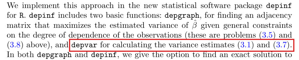
Corrected
  1. “(see, e.g., section 9.4.2 of Kellerer et al 13)”.
  2. “Theorem 2.7 of Chen and Shao [6]”.
  3. “[6] Chen LH, Shao QM (2004) Normal approximation under local dependence. The Annals of Probability 32(3):1985–2028”.
  4. “[19] Ogburn EL, VanderWeele TJ (2017) Vaccines, contagion, and social networks. The Annals of Applied Statistics 11(2):919–948”.

If reference [12] is kept for its other use on p. 2245, its entry should identify it as Appendix A of Knapsack Problems, pp. 483–493.

Crop of eight lines of text. A red box marks the number 12 at the start of a line, which completes '(see, e.g., section 9.4.2 of Kellerer et al 12)'. The second line of the crop ends 'See chapter 9 of Kellerer et al 13 for'.
P. 2245 (PDF p. 8). The marked reference number follows “section 9.4.2 of Kellerer et al” at the end of the line above; chapter 9 of the same book is cited as 13 four lines earlier.
Crop of three lines. A red box marks 'et al' in 'has been proven by, e.g., Theorem 2.7 of Chen et al [6].'
P. 2247 (PDF p. 10), after Lemma 2. The marked words follow the name of the first of two authors.
Crop of reference entries [5] and [6]. A red box marks 'et al' in '[6] Chen LH, Shao QM, et al (2004) Normal approximation under local dependence. The Annals of Probability 32(3):1985-2028'.
References, p. 2251 (PDF p. 14), entry [6].
Crop of reference entries [18] and [19]. A red box marks 'et al' in '[19] Ogburn EL, VanderWeele TJ, et al (2017) Vaccines, contagion, and social networks. The Annals of Applied Statistics 11(2):919-948'.
References, p. 2251 (PDF p. 14), entry [19].

The heading “Proof of 1.” should read “Proof of Corollary 1.”

Appendix A, p. 2249 (PDF p. 12), first proof heading

As printed

Proof of 1. Across all sample realizations, V^1(Am;Z)≥V^1(AO;Z)\widehat V_1(A^m;Z)\ge\widehat V_1(A^{\mathcal O};Z). Then by Proposition 1,

The problem

The heading omits the name of the result. The proof is that of Corollary 1. On p. 2245 the corollary is followed by the words “Proof is given in the Appendix”, the conclusion of display (A.1) is the statement of Corollary 1, and Proposition 1 has its proof in the main text.

Evidence a check of the printed page

I compared the page with Corollary 1 on p. 2245 and with Proposition 1 and its proof on pp. 2242–2244.

What survives

Nothing else changes. Whether the argument of (A.1) succeeds depends on Proposition 1, which is the subject of P011-E001.

Corrected

Proof of Corollary 1. Across all sample realizations, V^1(Am;Z)≥V^1(AO;Z)\widehat V_1(A^m;Z)\ge\widehat V_1(A^{\mathcal O};Z). Then by Proposition 1,

Crop of the heading 'Appendix A: Proofs', the first two lines of the first proof and the first line of display (A.1). A red box marks the heading 'Proof of 1.'
Appendix A, p. 2249 (PDF p. 12). The marked heading gives the number of the result without its name.

Clarity notes

Imprecise or ambiguous wording whose intended meaning is correct; not an error.

A dependency graph implies marginal independence relations; an edge permits dependence and does not require it.

Introduction, p. 2239 (PDF p. 2), second paragraph

As printed

“Dependency graphs are useful because they imply marginal non-independence relations in a set of variables, and the class of joint distributions compatible with any dependency graph is flexible.”

Intended meaning

The preceding sentence says that edges represent the possibility of probabilistic dependence. Definition 1 (p. 2240) is a one-way statement: if no edge joins two disjoint sets of vertices, then the outcomes of the two sets are independent. The graph therefore implies independence relations, and an edge implies nothing. For example, two independent Bernoulli variables joined by an edge satisfy Definition 1. The paper uses Definition 1 throughout, and no result depends on this sentence.

Corrected

“Dependency graphs are useful because they imply marginal independence relations in a set of variables, and the class of joint distributions compatible with any dependency graph is flexible.” Absent edges between disjoint sets of vertices imply independence of the corresponding outcomes; present edges permit dependence and do not require it.

Crop of six lines of the second paragraph of the introduction. A red box marks the word 'non-independence' in the phrase 'they imply marginal non-independence relations in a set of variables'. The preceding sentence reads 'Vertices represent individual units and edges represent the possibility of probabilistic dependence.'
Introduction, p. 2239 (PDF p. 2), second paragraph. The marked word should read “independence”.

Formal statements (Lean)

Formal results: 30 whole; 4 restricted; 7 refuted; 0 omitted.

Coverage concerns the identified claim under its stated assumptions. A checked proof establishes the formal statement; correspondence to the published text was reviewed by AI. Repository access is currently required to open the source links.

Each result links to its current formal statement and proof. “Whole” covers the identified claim under its assumptions; “restricted” covers the stated narrower scope; “refuted” gives a counterexample to the identified assertion; “omitted” has no current theorem. Any named published theorem used as a premise remains an assumption. Browse the formal results for this work.

Proposition 1, Corollary 1, the first sentence after Assumption 3, and Corollary 3, as printed (four-cycle blocks; the exact counterexample of the from-scratch check)

Proposition 1: p. 2242 (PDF p. 5); Corollary 1: p. 2245 (PDF p. 8); sentence after Assumption 3: p. 2246 (PDF p. 9); Corollary 3: p. 2248 (PDF p. 11)

Proposition 1, p. 2242 (PDF p. 5); Corollary 1, p. 2245 (PDF p. 8); sentence after Assumption 3, p. 2246 (PDF p. 9); Corollary 3, p. 2248 (PDF p. 11). The stated independent-sign four-cycle constructions satisfy Assumptions 1–3 and have a singleton compatible set, exact scaled variance 4 and mean bias -9/4, all stated finite moments, estimator limit 7/4, failure probabilities tending to one, and the exact all-alpha undercoverage formula. At alpha=0.05 its coverage limit is between 0.8045 and 0.8055. The a=3 construction has limit -5 and the stated positive-probability negative estimate. These counterexample facts refute the quoted printed assertions.

Historical component credits
  • Proved AronowAudit.P011.Wave1.cycle_counterexample_proof Historical support retained; baseline fidelity: ok; manifest: used; used in Solution; The component is a concrete counterexample, not an existential negation of every printed result. The clipped interval is exactly T1(f); printed coverage is no larger, and positivity holds with probability tending to one for a=3/2. No all-integer-n extension is needed because T1 specifies n=4m.
  • Proved AronowAudit.P011.cycle_covariance_algebra Historical support retained; baseline fidelity: ok; manifest: used; used in Solution; The matrix called covariance in the description is HH^T for independent unit-variance signs; the theorem is its required algebra certificate rather than a standalone probabilistic model claim.
  • Proved AronowAudit.P011.cycle_block_moments Historical support retained; baseline fidelity: ok; manifest: not used; not used in Solution; Not invoked separately: its helper or component is already supplied by the complete component rows used here.
  • Proved AronowAudit.P011.cycle_negative_realization Historical support retained; baseline fidelity: ok; manifest: used; used in Solution; This is the assigned deterministic value certificate; its actual positive probability is separately exported by R071-04, and the complete asymptotic assumptions are in R071-01.
  • Proved AronowAudit.P011.cycle_variance_formula Historical support retained; baseline fidelity: ok; manifest: not used; not used in Solution; Not invoked separately: its helper or component is already supplied by the complete component rows used here.
  • Proved AronowAudit.P011.uniform_integral Historical support retained; baseline fidelity: ok; manifest: used; used in Solution; Not invoked separately: its helper or component is already supplied by the complete component rows used here.
  • Proved AronowAudit.P011.saturated_graph_singleton Historical support retained; baseline fidelity: ok; manifest: used; used in Solution; Not invoked separately: its helper or component is already supplied by the complete component rows used here.
  • Proved AronowAudit.P011.uniform_function_product Historical support retained; baseline fidelity: ok; manifest: used; used in Solution; Not invoked separately: its helper or component is already supplied by the complete component rows used here.
  • Proved AronowAudit.P011.cycle_negative_probability Historical support retained; baseline fidelity: ok; manifest: used; used in Solution; Not invoked separately: its helper or component is already supplied by the complete component rows used here.

Proposition 1, Corollary 1, the first sentence after Assumption 3, and Corollary 3, as printed (path-of-three blocks; the validators' counterexample)

Proposition 1: p. 2242 (PDF p. 5); Corollary 1: p. 2245 (PDF p. 8); sentence after Assumption 3: p. 2246 (PDF p. 9); Corollary 3: p. 2248 (PDF p. 11)

Proposition 1, p. 2242 (PDF p. 5); Corollary 1, p. 2245 (PDF p. 8); sentence after Assumption 3, p. 2246 (PDF p. 9); Corollary 3, p. 2248 (PDF p. 11). Both independent-sign path-block laws satisfy Assumptions 1–3, the bound 27/5, the displayed mean/covariance matrices, singleton compatibility, all S/L/Q polynomials and block moments, the samplewise centering formula and the exact finite oracle expectation. For t=1 the estimator tends to 19/15 instead of 29/15 and its all-alpha coverage is strictly deficient; at alpha=0.05 its coverage limit is between 0.8873623230 and 0.8873623231. For t=2 it tends to -11/15, is negative with probability tending to one and has zero clipped coverage. Both are correctly specified OLS intercept examples. These facts refute the printed assertions.

Historical component credits
  • Proved AronowAudit.P011.Wave1.path_counterexample_proof Historical support retained; baseline fidelity: ok; manifest: used; used in Solution; The scope excludes separately assigned OLS and one-block certificates. Clipped coverage is the event explicitly requested by T2(e),(f), and t=1 undercoverage refutes the printed interval claim as its coverage cannot exceed clipped coverage.
  • Proved AronowAudit.P011.Wave1.path_block_moments_with_covariance Historical support retained; baseline fidelity: ok; manifest: used; used in Solution; The repaired statement explicitly exports the actual probability-law means and covariance, as well as the finite enumeration moments. Restricting t to {1,2} loses no case of T2.
  • Proved AronowAudit.P011.block_ols_representations Historical support retained; baseline fidelity: ok; manifest: used; used in Solution; For T2 the assigned component is its correctly specified regression and OLS-intercept identity, not a separate full-rank certificate; the concrete nonzero t and positive K ensure the usual inverse is meaningful. Star conclusions are additional mathematics and are not credited to an absent T15 target here.
  • Proved AronowAudit.P011.saturated_graph_singleton Historical support retained; baseline fidelity: ok; manifest: used; used in Solution; Not invoked separately: its helper or component is already supplied by the complete component rows used here.

Proposition 1, corrected (the limit of the oracle estimator with its mean term)

p. 2242 (PDF p. 5); the proof step replaced is on p. 2243 (PDF p. 6)

p. 2242 (PDF p. 5), replacing the proof step on p. 2243 (PDF p. 6). Under Assumption 2, without induced nesting of observed graphs, the scaled oracle converges to the scaled true variance plus the mean quadratic b_n. Its expectation remainder is bounded by 3(1+c2)²c1²/n and the sample variance converges to average marginal variance plus mean spread. Consistency is equivalent to b_n tending to zero; common means suffice. Conservativeness is equivalent to liminf b_n≥0; positive semidefiniteness suffices. The mean deviations sum to zero and |b_n|≤(1+c2)c1². The matrix I+A is positive semidefinite exactly for disjoint unions of cliques, with the stated clique-square variance formula.

Historical component credits
  • Proved AronowAudit.P011.revised_oracle_convergence Historical support retained; baseline fidelity: ok; manifest: not used; not used in Solution; The mathematical statement is faithful; the original row description calls this proved declaration a draft, which is stale status wording. No fidelity or severity verdict was changed after reading the record.
  • Proved AronowAudit.P011.revised_oracle_expectation Historical support retained; baseline fidelity: ok; manifest: not used; not used in Solution; The exact target constant and every k are exported; all covariance and integral moments are finite from Scaling rather than extra assumptions.
  • Proved AronowAudit.P011.revised_sample_variance Historical support retained; baseline fidelity: ok; manifest: not used; not used in Solution; The probability limit has a varying deterministic centre and places no common-unit-mean or homoskedasticity restriction on the family.
  • Proved AronowAudit.P011.oracle_mean_conditions Historical support retained; baseline fidelity: ok; manifest: not used; not used in Solution; Scaling implies |meanBias_k|<=(1+c2)c1^2, so the real liminf is finite and has its intended ordinary meaning. Both equivalences concern the oracle, as T3(iv),(v) require.
  • Proved AronowAudit.P011.clique_characterization Historical support retained; baseline fidelity: ok; manifest: used; used in Solution; Class labels C represent actual clique components; every finite equivalence relation has such natural labels, so this representation loses no graph. The sum is over attained labels and includes isolated vertices as singleton cliques.
  • Proved AronowAudit.P011.delta_sum_zero Historical support retained; baseline fidelity: ok; manifest: used; used in Solution; Not invoked separately: its helper or component is already supplied by the complete component rows used here.

The general expansion (F1) for quadratic-form estimators with a deterministic matrix, and the sufficient condition for conservativeness whatever the unit means

Replaces the argument of the proof of Proposition 1, pp. 2242–2244 (PDF pp. 5–7); not printed in the paper

Replaces the argument of the proof of Proposition 1, pp. 2242–2244 (PDF pp. 5–7); not printed in the paper. For deterministic symmetric matrices with uniformly bounded spectral norm, Assumption 2 gives both exact expectations, linear variance growth, and F1. PSD majorants give conservativeness for arbitrary unit means; nonnegative traces against admissible covariances suffice in place of the PSD difference condition, and only diagonal and true-edge entries enter those traces. The oracle matrix is PSD exactly for unions of cliques. Independent fair signs give the stated bounded-norm data-dependent counterexample. No nesting of observed graphs or monotonicity of observed sizes is required.

Historical component credits
  • Proved AronowAudit.P011.quadratic_expectation Historical support retained; baseline fidelity: ok; manifest: used; used in Solution; The explicit L2 condition is implied by Assumption 2 because each weighted coordinate is a.s. bounded about the finite real beta; it is not an additional restriction on the target cases. Removing the other Scaling hypotheses extends the exact identity. No verdict changed after reading the record.

  • Proved AronowAudit.P011.deterministic_quadratic_expansion Historical support retained; baseline fidelity: ok; manifest: not used; not used in Solution; Scaling supplies finite moments and bounded covariance; the moving probability centre is exactly the bracket divided by n. Deterministic M and genuine Euclidean operator norm are essential and match T4. This row does not separately establish the cross-referenced clique characterization in the target narrative.
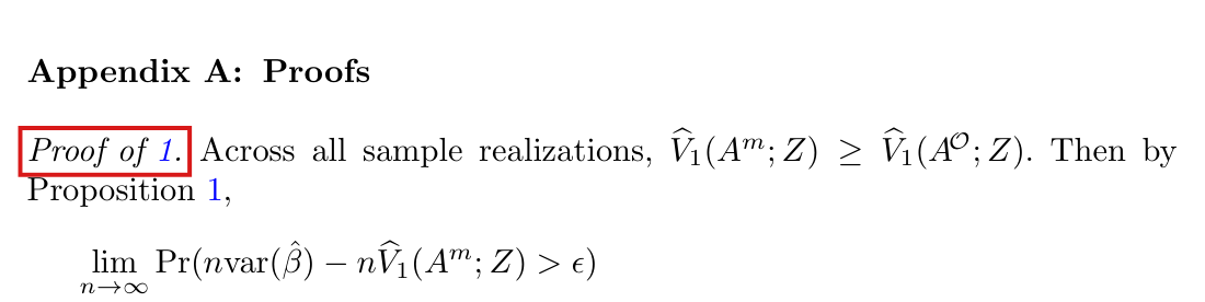
  • Counterexample proved AronowAudit.P011.data_dependent_expansion_failure Historical support retained; baseline fidelity: ok; manifest: used; used in Solution; Role: counterexample witness to extending the corrected deterministic F1 expansion to data-dependent M, not a refutation of a printed paper assertion. The sign law gives C=I, delta=0 and n Var(betaHat)=1, so every hypothesis of the proposed extension is met. No separate full-negation theorem is claimed.

Corollary 1, corrected for a partly known graph: the degree-corrected estimator, the closed-form bound, and their minimum (Proposition 1A of the correction, as strengthened by the check)

Replaces Corollary 1, p. 2245 (PDF p. 8), and the use of (3.1) in programs (3.5)–(3.6), pp. 2244–2245 (PDF pp. 7–8); not printed in the paper

Replaces Corollary 1, p. 2245 (PDF p. 8), and the use of (3.1) in programs (3.5)–(3.6), pp. 2244–2245 (PDF pp. 7–8); not printed in the paper. The degree-corrected estimator and Young bound satisfy all finite decompositions, PSD and nonnegativity conclusions, norm and oracle bounds, affine edge-objective and attained-optimum identities, and the constant-cap and regular-graph formulas, including zero degree. Under Assumption 2 and valid constraints the corrected oracle, sample maximizer, Young bound, and their stated minimum are conservative for arbitrary unit means, with no uniform bound on supplied degree caps. Common caps give the same conclusion for (3.9), without homoskedasticity. No nesting of observed graphs or monotonicity of observed sizes is required.

Historical component credits
  • Proved AronowAudit.P011.corrected_finite Historical support retained; baseline fidelity: ok; manifest: used; used in Solution; The all-compatible-A affine identity gives the optimal-value formula upon specializing to the actual maximizer of the same objective; the factor 2 correctly converts unordered program edges to ordered adjacency sums. The Assumption-2 norm bound and maximizing domination belong to corrected_asymptotic, not this distribution-free finite component.
  • Proved AronowAudit.P011.corrected_asymptotic Limited support; baseline fidelity: narrower; manifest: not used; not used in Solution; {'source': 'adjudication+second review', 'adjudicator': 'P011_CorrectedAsymptoticCompletion.lean:162 exports the norm bound, maximizer domination and n-scaled conservativeness, but none of the four pointwise nonnegativity conclusions expressly promised by the row. Its constant-cap implication at :176 concludes only Conservative(V2prime), not the advertised finite equality VYoung = V2prime from T5(f); the PSD-majorant portion of the cited T5(b) is also absent. Conservative, defined at P011_Audit.lean:208 as a tail-probability limit, does not contain these finite assertions. P011_Audit.lean:2070 and :2648 establish finite ingredients separately, which confirms that the defect is missing conclusions rather than an invalid conservativeness result or an added degree-bound assumption.', 'suggested_fix': 'Add the T5(b) PSD-majorant conclusion, samplewise nonnegativity of the corrected oracle, corrected maximum, Young bound and their minimum, and the samplewise equality VYoung = V2prime when truncated caps are constant across units. These conjuncts can use corrected_matrix_majorant and corrected_finite without adding hypotheses.', 'second_review': "Of the explicitly credited T5(b),(c),(h),(i), T5(b) requires the PSD diagonal majorant difference as well as the norm bound; P011/P011_CorrectedAsymptoticCompletion.lean:162 exports the norm bound, domination and conservativeness but omits that PSD conclusion. The omission is mathematically elementary: correctedMatrix at P011/P011_Audit.lean:90 differs from oracleMatrix by diag(t_i d_i^A), and degreeCorrection at :86 is nonnegative because each positive truncated degree is an integer at least one. The description's additional samplewise nonnegativity and constant-cap equality promises concern finite material beyond these credited clauses, with equality belonging to T5(f), and should be narrowed or explicitly added. Retain a statement repair for T5(b), but classify its missing diagonal-positivity assertion as minor rather than major.", 'severity': 'minor'}
  • Proved AronowAudit.P011.adjacency_quadratic_bound Historical support retained; baseline fidelity: ok; manifest: used; used in Solution; Not invoked separately: its helper or component is already supplied by the complete component rows used here.
  • Proved AronowAudit.P011.young_bound_finite Historical support retained; baseline fidelity: ok; manifest: used; used in Solution; Not invoked separately: its helper or component is already supplied by the complete component rows used here.
  • Proved AronowAudit.P011.quadratic_add Historical support retained; baseline fidelity: ok; manifest: used; used in Solution; Not invoked separately: its helper or component is already supplied by the complete component rows used here.
  • Proved AronowAudit.P011.quadratic_diagonal Historical support retained; baseline fidelity: ok; manifest: used; used in Solution; Not invoked separately: its helper or component is already supplied by the complete component rows used here.
  • Proved AronowAudit.P011.corrected_diagonal_bounds Historical support retained; baseline fidelity: ok; manifest: used; used in Solution; Not invoked separately: its helper or component is already supplied by the complete component rows used here.
  • Proved AronowAudit.P011.corrected_matrix_majorant Historical support retained; baseline fidelity: ok; manifest: used; used in Solution; The matrix difference is the nonnegative diagonal correction by the definition of correctedMatrix; symmetry and nonnegative quadratic forms are real PSD, not a proposition assumed to mean the desired conclusion.
  • Proved AronowAudit.P011.ordered_pair_sum Historical support retained; baseline fidelity: ok; manifest: used; used in Solution; Not invoked separately: its helper or component is already supplied by the complete component rows used here.
  • Proved AronowAudit.P011.graph_laplacian_identity Historical support retained; baseline fidelity: ok; manifest: used; used in Solution; Not invoked separately: its helper or component is already supplied by the complete component rows used here.
  • Proved AronowAudit.P011.adjacency_upper_quadratic Historical support retained; baseline fidelity: ok; manifest: used; used in Solution; Not invoked separately: its helper or component is already supplied by the complete component rows used here.
  • Proved AronowAudit.P011.degree_weight_sum Historical support retained; baseline fidelity: ok; manifest: used; used in Solution; Not invoked separately: its helper or component is already supplied by the complete component rows used here.
  • Proved AronowAudit.P011.psd_diagonal Historical support retained; baseline fidelity: ok; manifest: used; used in Solution; Not invoked separately: its helper or component is already supplied by the complete component rows used here.
  • Proved AronowAudit.P011.psd_add Historical support retained; baseline fidelity: ok; manifest: used; used in Solution; Not invoked separately: its helper or component is already supplied by the complete component rows used here.
  • Proved AronowAudit.P011.graph_laplacian_psd Historical support retained; baseline fidelity: ok; manifest: used; used in Solution; Not invoked separately: its helper or component is already supplied by the complete component rows used here.

Proposition 1, corrected for a known graph: the positive-part estimator (F4)

Replaces the use of V^1(AO;Z)\widehat V_1(A^{\mathcal O};Z) when the dependency graph is known, p. 2242 (PDF p. 5); not printed in the paper

replaces the known-graph use of (3.1), p. 2242 (PDF p. 5). Spectral clipping is a PSD majorant with the degree norm bound, dominates both the oracle estimate and zero, and is asymptotically conservative under Assumption 2. It is the unique nearest PSD matrix in Frobenius norm, but is neither a least Loewner majorant nor affine in the adjacency entries. The four-cycle spectrum, quadratic identities, alternative majorant, exact expectation 4-12/n and limit 4 are included.

Historical component credits
  • Proved AronowAudit.P011.positive_part_finite Historical support retained; baseline fidelity: ok; manifest: used; used in Solution; Exports minimum distance and all finite bounds in its designated scope. Uniqueness and nonaffinity are separately credited rows R073-08 and R073-09.
  • Proved AronowAudit.P011.positive_part_conservative Historical support retained; baseline fidelity: ok; manifest: not used; not used in Solution; The probability law on real coordinate space represents arbitrary real outcome laws; bounded weighted outcomes guarantee the required moments. The public correction summary accurately states this n-scaled result.
  • Proved AronowAudit.P011.cycle_positive_identity Historical support retained; baseline fidelity: ok; manifest: used; used in Solution; The designated finite algebraic component is exact, with no restriction to centered or realizable vectors.
  • Proved AronowAudit.P011.Wave1.positive_part_cycle_claims_proof Historical support retained; baseline fidelity: ok; manifest: used; used in Solution; Faithful to the expressly assigned majorant and expectation/limit component. The true-variance identity remains a target-level coverage gap, not a new hypothesis on this row.
  • Proved AronowAudit.P011.cycle_spectral_certificate Historical support retained; baseline fidelity: ok; manifest: used; used in Solution; As a certificate, the explicit orthogonal eigendecomposition and clipped candidate give the target eigenvalues and alternating eigenvector. It makes no independent asymptotic claim.
  • Proved AronowAudit.P011.cycle_majorant_certificate Historical support retained; baseline fidelity: ok; manifest: used; used in Solution; Not invoked separately: its helper or component is already supplied by the complete component rows used here.
  • Proved AronowAudit.P011.cycle_clipped_entries Withdrawn support; baseline fidelity: wrong_credit; manifest: used; used in Solution; Excluded: final_status is wrong_credit; no independent target credit is taken.
  • Proved AronowAudit.P011.positive_part_nearest_unique Historical support retained; baseline fidelity: ok; manifest: used; used in Solution; This is the usual uniqueness characterization once the separate minimum-distance result is available.
  • Proved AronowAudit.P011.positive_part_objective_nonaffine Historical support retained; baseline fidelity: ok; manifest: used; used in Solution; A single fixed-data nonaffinity witness suffices to rule out a generally affine objective. The row does not claim that every data vector gives a nonaffine function.
  • Proved AronowAudit.P011.positive_part_psd Historical support retained; baseline fidelity: ok; manifest: used; used in Solution; Not invoked separately: its helper or component is already supplied by the complete component rows used here.
  • Proved AronowAudit.P011.positive_part_of_psd Historical support retained; baseline fidelity: ok; manifest: used; used in Solution; Not invoked separately: its helper or component is already supplied by the complete component rows used here.
  • Proved AronowAudit.P011.variance_form_oracle Historical support retained; baseline fidelity: ok; manifest: used; used in Solution; Not invoked separately: its helper or component is already supplied by the complete component rows used here.

Corollaries 1 and 3 in the degree-only case: the maximized V^1\widehat V_1 when no edges are known (Proposition 1B of the correction, as strengthened by the check)

Corollary 1, p. 2245 (PDF p. 8); the degree-only case is the one described on p. 2248 (PDF p. 11)

Corollary 1, p. 2245 (PDF p. 8), and the degree-only case on p. 2248 (PDF p. 11). The degree identity and both fixed-cap finite comparisons hold. Under Assumption 2, the degree-only maximum is conservative and has conservative clipped Wald coverage, even for unbounded supplied caps; residuals are bounded by 2c1 almost surely. For independent fair signs with caps n-1, every nonconstant sample has exactly the two residual-sign cliques as optimizer, while the exact estimates converge unscaled to 1/2 and 1, respectively.

Historical component credits
  • Proved AronowAudit.P011.Wave1.degree_only_finite_proof Historical support retained; baseline fidelity: ok; manifest: used; used in Solution; The simultaneous maximizers exclude no degree/data instance. D=0 gives the intended exact equalities rather than an inconsistent or negative-bound premise.
  • Proved AronowAudit.P011.Wave1.degree_only_conservative_proof Historical support retained; baseline fidelity: ok; manifest: not used; not used in Solution; Empty recruitment is part of the corrected T7(c) claim itself. Supplied bounds may grow arbitrarily; no selector measurability premise or common-unit-mean restriction is added.
  • Proved AronowAudit.P011.Wave1.unbounded_caps_gap_proof Historical support retained; baseline fidelity: ok; manifest: used; used in Solution; Faithful to the assigned values/limits component. The theorem does not export the separate assertion that every optimizer has precisely the two-clique structure when both signs occur; that is a target coverage gap.
  • Proved AronowAudit.P011.degree_only_edge_identity Historical support retained; baseline fidelity: ok; manifest: used; used in Solution; All graph types, ordered versus unordered sums, and natural-to-real degree coercions agree with the finite identity.

Corollaries 1 and 3, corrected

Corollary 1: p. 2245 (PDF p. 8); Corollary 3: p. 2248 (PDF p. 11); the sentence on p. 2246 (PDF p. 9) is deleted

Corollary 1, p. 2245 (PDF p. 8), and Corollary 3, p. 2248 (PDF p. 11); the homoskedasticity sentence on p. 2246 (PDF p. 9) is deleted. Under Assumption 2, every estimator in the corrected list has one-sided asymptotic variance control and conservative clipped Wald coverage: the four corrected/Young estimators under valid constraints, spectral clipping, the degree-only original maximum, and the oracle or original maximum when the mean-bias limit inferior is nonnegative. Equal unit means and disjoint clique graphs imply that condition. The first two branches are nonnegative in every sample. The homoskedastic cycle and path counterexamples show why no such conclusion holds for the unrestricted original estimator with known edges.

Historical component credits
  • Proved AronowAudit.P011.Wave1.revised_corollaries_proof Historical support retained; baseline fidelity: ok; manifest: not used; not used in Solution; CorrectedClass enumerates explicit estimators and their target-prescribed admissibility conditions; it does not contain Conservative or ConservativeCoverage as fields. The quantile and clipping agree with corrected T8, and Scaling bounds meanBias, so its real liminf has the ordinary bounded-sequence meaning. The row proves the positive revised corollary pair, not the cross-referenced failures of the original printed corollaries.
  • Proved AronowAudit.P011.clipped_truncation Historical support retained; baseline fidelity: ok; manifest: not used; not used in Solution; Not invoked separately: its helper or component is already supplied by the complete component rows used here.

The residual-centred version of V^1\widehat V_1 when a mean model is available, with the regularity it needs

Replaces the centring at β^\hat\beta in (3.1) and (3.5), pp. 2242 and 2244 (PDF pp. 5 and 7), for the regression example of Section 2, pp. 2240–2241 (PDF pp. 3–4); not printed in the paper

replaces centring in (3.1) and (3.5), pp. 2242 and 2244 (PDF pp. 5 and 7), for the regression example, pp. 2240–2241 (PDF pp. 3–4); corrected statement, not printed. Under Assumption 2 and the correct bounded finite-dimensional mean model, root-n coefficient estimation gives zero-mean residuals with covariance C, the three stated stochastic norm rates, oracle consistency and maximal-estimator conservativeness. The finite symmetric quadratic perturbation bound holds. Bounded residuals and prediction error o_p(sqrt(n)) also suffice; a misspecified model adds the quadratic mean term. The independent-sign OLS example satisfies Assumption 2 with exact scaled variance 2, but has intercept variance n/2+1/(2n), residual expectation n+2-7/n (17/4 and 73/8 at n=4 and 8) and fails consistency, with the explicit slope weights and samplewise residual sum. No observed-graph nesting is required.

Historical component credits
  • Proved AronowAudit.P011.residual_perturbation Historical support retained; baseline fidelity: ok; manifest: used; used in Solution; The statement matches the assigned finite auxiliary component; no hidden result assumption or problematic totalization is used.
  • Proved AronowAudit.P011.Wave1.residual_root_n_proof Historical support retained; baseline fidelity: ok; manifest: not used; not used in Solution; No OLS identity, full rank or design nonsingularity is assumed: the target allows any estimator with the stated root-n rate.
  • Proved AronowAudit.P011.Wave1.residual_prediction_stability_proof Historical support retained; baseline fidelity: ok; manifest: not used; not used in Solution; MeanModel integrability and estimator measurability make the target’s finite means and random estimator explicit; neither adds an exceptional-case exclusion.
  • Proved AronowAudit.P011.Wave1.misspecified_residual_limit_proof Historical support retained; baseline fidelity: ok; manifest: not used; not used in Solution; Only T9(e) is credited. No limit or nonnegativity of its moving bias is assumed; raw zero-weight coordinates need not be bounded.
  • Proved AronowAudit.P011.Wave1.residual_missing_regularity_proof Historical support retained; baseline fidelity: ok; manifest: used; used in Solution; This is a counterexample to the residual correction without regularity, not a refutation of a printed residual theorem: the target itself is a corrected statement. The actual witness has n Var(betaHat)=2 identically, so its failure to approach 2 is also failure to track the true scaled variance.

Why consistency cannot be kept for arbitrary unit means: no estimator is consistent at the nn-scaled level over all bounded mean patterns

Bears on the abstract, p. 2238 (PDF p. 1) ("We establish the consistency of an oracle variance estimator when a dependency graph is known") and Proposition 1, p. 2242 (PDF p. 5); not printed in the paper

bears on the abstract, p. 2238 (PDF p. 1), and Proposition 1, p. 2242 (PDF p. 5); corrected statement, not printed. For every a,b>0 the independent fixed-sign-mean and random-sign-mixture models satisfy all scaling assumptions, have the stated finite means and scaled variances b² and a²+b², and obey the exact finite mixture identity. No statistic is scaled consistent in all these models, and mixture conservativeness prevents consistency in every fixed mean pattern. Consequently no law-independent observed-data variance rule is universally scaled consistent. The zero statistic is unscaled consistent under Assumption 2. Extra sampling-design information can permit unbiased variance estimation: independent half-probability inclusion of population values 1 gives betaHat=average(2I) and the unbiased estimator average(2I)/n.

Historical component credits
  • Proved AronowAudit.P011.Wave1.universal_consistency_impossible_proof Historical support retained; baseline fidelity: ok; manifest: used; used in Solution; The quantifier over one fixed infinite pattern precedes the limit, and the same statistic is used under every law. The impossibility over all admissible models follows by restriction to these subfamilies, whose ancillary data agree.
  • Proved AronowAudit.P011.mixture_finite_moments Historical support retained; baseline fidelity: ok; manifest: used; used in Solution; The broader parameter range is mathematically harmless. Finite support ensures genuine moments, so integral defaults do not cause these equalities.

Proof of Proposition 2, the consistency claimed for the auxiliary oracle estimator V^2∗(AO;Z)\widehat V_2^*(A^{\mathcal O};Z), as printed

p. 2246 (PDF p. 9), proof of Proposition 2

p. 2246 (PDF p. 9), proof of Proposition 2. The alternating-means counterexample refutes the quoted auxiliary proof step both as printed with < epsilon and under the intended > epsilon consistency reading. It establishes the exact finite moments and both failure limits, while preserving Proposition 2's one-sided conservativeness conclusion.

Historical component credits
  • Proved AronowAudit.P011.Wave1.alternating_counterexample_proof Historical support retained; baseline fidelity: ok; manifest: used; used in Solution; This witness meets both the printed less-than event and the intended greater-than event tests at the specified positive thresholds. It also proves the valid one-sided Proposition 2 conclusion.
  • Proved AronowAudit.P011.Wave1.alternating_finite_moments_proof Historical support retained; baseline fidelity: ok; manifest: used; used in Solution; This is a finite supporting component of a counterexample, not a standalone asymptotic refutation; R074-06 and R074-08 supply the remaining components.
  • Proved AronowAudit.P011.auxiliary_empty_identity Historical support retained; baseline fidelity: ok; manifest: used; used in Solution; The general modelling paragraph describes the project’s asymptotic framework, whereas this row is only the exact finite identity and requires none of those extra asymptotic conditions.

Proposition 2 with its proof corrected (a direct one-sided argument that replaces the auxiliary consistency step)

p. 2246 (PDF p. 9)

p. 2246 (PDF p. 9). Under Assumptions 2 and 3, the homoskedastic oracle estimator satisfies the entire finite moment, covariance and scalar gap chain, the explicit tail bound 4(1+c2)^3 c1^4/(n epsilon^2), and one-sided asymptotic conservativeness. Unit means may differ, early common variances may vanish, and neither the mean spread nor the common variance needs a limit.

Historical component credits
  • Proved AronowAudit.P011.homoskedastic_repair Historical support retained; baseline fidelity: ok; manifest: not used; not used in Solution; No equal-unit-mean, positive early variance, auxiliary-estimator consistency or separate mean-spread limit is assumed. The intermediate chain inequalities in T12(ii),(iii) follow algebraically from the exported finite bounds and definitions.
  • Proved AronowAudit.P011.one_sided_algebra Historical support retained; baseline fidelity: ok; manifest: not used; not used in Solution; The statement matches the assigned finite auxiliary component; no hidden result assumption or problematic totalization is used.
  • Proved AronowAudit.P011.centered_sum_zero Historical support retained; baseline fidelity: ok; manifest: not used; not used in Solution; Not invoked separately: its helper or component is already supplied by the complete component rows used here.
  • Proved AronowAudit.P011.sample_variance_centering Historical support retained; baseline fidelity: ok; manifest: not used; not used in Solution; Not invoked separately: its helper or component is already supplied by the complete component rows used here.

The complexity of programs (3.5), (3.6) and (3.8), corrected: exact solution by reduction to maximum-weight matching

p. 2245 (PDF p. 8), the two paragraphs after program (3.6); programs (3.5) p. 2244 (PDF p. 7), (3.6) p. 2245 (PDF p. 8), (3.8) p. 2246 (PDF p. 9)

p. 2245 (PDF p. 8), the two paragraphs after program (3.6); programs (3.5) p. 2244 (PDF p. 7), (3.6) p. 2245 (PDF p. 8), (3.8) p. 2246 (PDF p. 9). The finite degree-constrained optimization problem reduces to a matching gadget with exact decoding, counts, and two attained numerical instances.

Historical component credits
  • Proved AronowAudit.P011.Wave1.matching_reduction_proof Historical support retained; baseline fidelity: ok; manifest: used; used in Solution; The feasible optional decomposition is existential rather than written with unique existence; forced/optional disjointness makes its witness uniquely S minus F. No time-complexity claim is assigned to this row.
  • Proved AronowAudit.P011.Wave1.corrected_polynomial_size_matching_reduction Withdrawn support; baseline fidelity: wrong_credit; manifest: not used; not used in Solution; Excluded: final_status is wrong_credit; no independent target credit is taken.
  • Proved AronowAudit.P011.matching_gadget_exact_counts Historical support retained; baseline fidelity: ok; manifest: used; used in Solution; This is only the exact finite-cardinality component; the tagged types really are finite, including the empty cases.
  • Proved AronowAudit.P011.Wave1.matching_exact_instances_proof Historical support retained; baseline fidelity: ok; manifest: used; used in Solution; The existential matching witnesses certify attained optima and are accompanied by universal optimality; the result is not just an unattained upper bound.

The linear-programming relaxation of programs (3.5), (3.6) and (3.8), corrected description: an upper bound that need not be attained by a graph

p. 2245 (PDF p. 8), after program (3.6); p. 2248 (PDF p. 11), "Upper bounds for the variance estimates can be obtained by solving a relaxed form of the programs (3.5) and (3.8)"; Appendix B, p. 2250 (PDF p. 13)

p. 2245 (PDF p. 8), after program (3.6); p. 2248 (PDF p. 11), "Upper bounds for the variance estimates can be obtained by solving a relaxed form of the programs (3.5) and (3.8)"; Appendix B, p. 2250 (PDF p. 13). Certified relaxed bounds control integer objectives and both variance estimators, and the six-unit and triangle examples have strictly fractional optima.

Historical component credits
  • Proved AronowAudit.P011.relaxation_upper_bound Historical support retained; baseline fidelity: ok; manifest: used; used in Solution; The universal relaxed-bound premise is the certified input specified by the target; it is not the desired integer bound assumed as a hypothesis. Compatibility is the actual graph feasibility condition.
  • Proved AronowAudit.P011.relaxation_gaps Historical support retained; baseline fidelity: ok; manifest: used; used in Solution; These are witnesses for the corrected nonintegrality claim, with upper bounds and attainment both exported. The three-unit unit-weight relaxed objective 3/2 is the ordered program value 3.

The claim that the general estimator, applied with raw outcomes to an OLS coefficient under forced recruitment edges, is conservative (package README and vignette; Corollary 1 for the regression example of Section 2)

Package README.md, line 3, and vignettes/replication.Rmd, lines 100–105 (staged/packages/depinf/jrzubizarreta-depinf-f11933a); the results invoked are Corollary 1, p. 2245 (PDF p. 8), and the regression example, pp. 2240–2241 (PDF pp. 3–4)

package README line 3 and vignette lines 100–105; Section 2, pp. 2240–2241; Corollary 1, p. 2245. The two correctly specified binary star regressions satisfy the standing assumptions, full-rank design identities, independent Bernoulli leaf and conditional centre laws, and saturated binary and fractional constraints. Their raw maximal variance estimates converge below and above the true variance, respectively. The first has ratio 8/9, underestimation probability tending to one, and the stated strict undercoverage for both the clipped and printed-domain intervals; negative estimates vanish in probability. The explicit mean offsets have the stated negative and positive quadratics, while true-error products converge to the true variance in both models.

Historical component credits
  • Proved AronowAudit.P011.Wave1.star_counterexample_proof Limited support; baseline fidelity: narrower; manifest: used; used in Solution; {'source': 'adjudication+second review', 'adjudicator': "GLP011B4.lean:696 states the star-law counterexample, its binary-compatible-graph singleton, scaled variance limits and undercoverage, but contains no regression design, MeanModel assertion or OLS-intercept identity. Consequently it does not establish the correctly specified regressions in T15(a),(e) that the row's promised T15(a)-(f) package includes. The binary singleton at :707 also does not state T15(b)'s singleton for the real-valued LP relaxation. Those missing connections occur separately in P011_BlockOLSCompletion.lean:245 and P011_StarCompletion.lean:96; zero-based indexing and clipped coverage introduce no material difference here.", 'suggested_fix': 'Add conjuncts for both displayed two-column star designs, their Gram and mean-model identities, and their OLS intercepts equalling the sample mean. Also assert that every feasible real LP edge-weight vector equals the true adjacency vector, for both star families; the existing separate OLS and relaxation results supply these connections.', 'second_review': 'T15(a),(e) specify correctly specified two-column regressions whose OLS intercept is the sample mean, and T15(b) also requires the LP relaxation to have a single feasible point. P011/Wave1/Gap/GLP011B4.lean:696 exports the outcome-law counterexample and its limits, but its singleton at :707 concerns only Boolean graphs, and starModel at P011/P011_Audit.lean:424 contains no regression design or OLS assertion. The missing regression identities and real-valued relaxation singleton are substantive links to the credited regression counterexample, separately stated at P011/P011_BlockOLSCompletion.lean:245 and P011/P011_StarCompletion.lean:96. Conjoining those links repairs the statement without changing the counterexample.', 'severity': 'major'}
  • Proved AronowAudit.P011.star_mean_terms Historical support retained; baseline fidelity: ok; manifest: used; used in Solution; The signs are exact block calculations; their stochastic meaning uses the explicitly constructed mean vectors in the companion rows.
  • Proved AronowAudit.P011.block_ols_representations Historical support retained; baseline fidelity: ok; manifest: used; used in Solution; The path clauses are additional to the star component credited here. Positive K and the specified nonzero centered covariates exclude singular-inverse fallback.
  • Proved AronowAudit.P011.star_relaxation_singleton Historical support retained; baseline fidelity: ok; manifest: used; used in Solution; The row concerns only LP constraints, and does not claim an estimator or stochastic conclusion.
  • Proved AronowAudit.P011.saturated_graph_singleton Historical support retained; baseline fidelity: ok; manifest: used; used in Solution; This is the general finite constraint lemma used by the star witness, not a standalone stochastic counterexample.

What can be claimed for an OLS coefficient: the condition for the raw-outcome estimator, and the residual-based estimator with the design conditions it needs

Regression example, pp. 2240–2241 (PDF pp. 3–4); (3.1), p. 2242 (PDF p. 5); package vignette vignettes/replication.Rmd, lines 100–105

regression example, pp. 2240–2241; (3.1), p. 2242; package vignette lines 100–105. Corrected claim. For a full-rank fixed-design OLS coefficient, weighted unit means and their offsets have the exact stated formulas. Under Assumption 2 the raw oracle has the moving mean-bias limit, is consistent exactly when that bias tends to zero, and is conservative exactly when its liminf is nonnegative. With valid constraints this condition suffices for every compatible maximum, but is not necessary in general, as the independent binary-star regression with empty recruitment demonstrates. Equal weighted unit means suffice for consistency and maximal conservativeness. Every design-space outcome shift leaves fitted residual products and all residual objectives unchanged and has the stated effect on raw centred products. With an intercept, constant shifts preserve slopes and residual objectives, but can change raw slope variance, as an explicit two-point example shows. Under Assumption 2, fixed dimension, uniformly bounded rows and outcomes, and a uniformly coercive normalized Gram matrix, OLS has the root-n rate. The displayed normalized residual perturbation inequality holds and its right side tends to zero in probability; the residual oracle is consistent and every compatible residual maximum is conservative. Deterministic coefficients and targets may vary with sample size. The usual measure-theoretic conditions are assumed.

Historical component credits
  • Proved AronowAudit.P011.Wave1.ols_repair_proof Limited support; baseline fidelity: narrower; manifest: not used; not used in Solution; {'source': 'adjudication+second review', 'adjudicator': "GLP011B5.lean:356 makes Scaling a premise of the entire conjunction, including the finite mean formula at :361 and exact shift identities at :364. T16(i)'s finite mean identity and T16(ii)'s shift identities require the full-rank integrable mean model, not Assumption 2; Gaussian-error regressions and deterministic regressions provide substantive excluded cases. The asymptotic clause at :369 exports the root-n rate, residual-oracle consistency and maximal conservativeness, but omits T16(iii)'s displayed normalized quadratic perturbation inequality and the convergence of its right-hand side. The separately stated finite identities and perturbation lemmas do not restore these conclusions to this credited declaration.", 'suggested_fix': 'State the exact mean and shift identities for a finite positive sample size under full rank, MeanModel and the OLS weight identity alone; require Scaling only for the asymptotic clauses. Under the additional bounds of T16(iii), also export the displayed inequality with factor 1+c2 and convergence in probability of its right-hand side to zero.', 'second_review': "T16(i)'s exact mean formula and T16(ii)'s shift identities require the full-rank integrable mean model, whereas P011/Wave1/Gap/GLP011B5.lean:356 assumes Scaling for the entire conjunction. Scaling at P011/P011_Audit.lean:187 adds uniformly bounded weighted outcomes and positive limiting scaled variance, excluding, for example, Gaussian-error and deterministic full-rank regressions from these finite identities. The asymptotic conclusion at GLP011B5.lean:369 also omits T16(iii)'s displayed normalized perturbation inequality and convergence of its right-hand side. Separate the finite identities from Scaling and export the perturbation conclusion under the stated asymptotic design bounds.", 'severity': 'major'}

Display (3.3), corrected, with the leading term of (3.4)

(3.3): p. 2243 (PDF p. 6); (3.4): pp. 2243–2244 (PDF pp. 6–7)

(3.3), p. 2243; (3.4), pp. 2243–2244. The corrected pair and fourth moments and constant-centering covariance expansion hold on their separate integrable moment domains.

Historical component credits
  • Proved AronowAudit.P011.Wave1.corrected_covariance_expansion_moments Historical support retained; baseline fidelity: ok; manifest: used; used in Solution; {'source': 'adjudication', 'decision': 'rejected', 'what': 'P011/Wave1/Gap/Fid2P011.lean:423 gives independently conditional weighted-pair, weighted-fourth, constant-centering, raw-pair and raw-fourth identities. These antecedents require the individual moments displayed in the respective T17 formulas, rather than global raw L4, and the random-centering branches explicitly identify covOf with ordinary covariance. Grouping the sixteen terms and the two pair blocks changes no coefficients or cases; the constant-centering moment domain likewise justifies ordinary covariance, and the asymptotic remainder is outside this target.'}
  • Proved AronowAudit.P011.fourth_polynomial Historical support retained; baseline fidelity: ok; manifest: used; used in Solution; The complete moment-domain result already supplies the fourth-moment identity; this polynomial row is not needed separately.
  • Proved AronowAudit.P011.covariance_expansion_linear Historical support retained; baseline fidelity: ok; manifest: not used; not used in Solution; The complete moment-domain result already supplies the covariance expansion; this abstract algebra row is not needed separately.

Display (3.3), as printed

p. 2243 (PDF p. 6)

The printed claim is false: The constant-outcome witness gives true covariance zero, printed values 9/4 and 93009/16, the named bracket-only repair -70, and fully corrected value zero. (3.3), p. 2243.

Historical component credits
  • Counterexample proved AronowAudit.P011.printed_expansion_counterexample Historical support retained; baseline fidelity: ok; manifest: used; used in Solution; {'source': 'adjudication', 'decision': 'rejected', 'what': "P011/P011_Audit.lean:1260 gives the target's probability-one constant witness and the exact values 0, 9/4, 93009/16, -70 and 0. The bracket-only repair is represented by precisely the evaluated rational expression displayed in T18(d), while the other printed and corrected expressions retain their moment definitions. A Dirac probability law is a legitimate witness to the finite algebraic failure; the constant witness does not rely on a zero-measure convention."}

Proof of Proposition 2, the convergence display, with the inequality corrected

p. 2246 (PDF p. 9)

proof of Proposition 2, p. 2246. For positive common variance under Assumptions 2 and 3, the auxiliary error is k times the sample-variance error, where k is the true scaled variance divided by the common variance and lies between zero and 1+c2. The sample-variance remainder after subtracting between-unit mean spread converges to zero in probability. Vanishing mean spread, in particular equal weighted unit means, suffices for auxiliary consistency. The explicit alternating-mean independent-sign family satisfies all these standing assumptions with positive common variance, yet its mean spread tends to one and its auxiliary error exceeds 1/2 with probability tending to one.

Historical component credits
  • Proved AronowAudit.P011.auxiliary_corrected_display Historical support retained; baseline fidelity: ok; manifest: used; used in Solution; All three positive assertions of the repaired display are covered, including the explicitly stated positive common variance. This theorem gives the sufficient mean-spread condition; the separate observation that sign repair alone fails is not independently refuted by any T19 row in this chunk.

Proof of Proposition 2, the convergence display as printed (with <ϵ< \epsilon)

p. 2246 (PDF p. 9)

The printed claim is false: Fair signs refute the printed limit-zero display and give its exact inside-event probabilities and limit one. proof of Proposition 2, p. 2246.

Historical component credits
  • Counterexample proved AronowAudit.P011.Wave1.printed_sign_counterexample_full_printed_negation Historical support retained; baseline fidelity: ok; manifest: used; used in Solution; The negated contract keeps the printed strict-inside event and zero limit. Pairwise-correlation and observed-coordinate conventions lose no cases relevant to the all-observed edgeless witness; no conditional published theorem is assumed.
  • Proved AronowAudit.P011.auxiliary_empty_identity Historical support retained; baseline fidelity: ok; manifest: used; used in Solution; The equality is samplewise and independent of moment assumptions, including if totalized covariance values are otherwise uninformative.
  • Proved AronowAudit.P011.uniform_coordinate_dependency Historical support retained; baseline fidelity: ok; manifest: used; used in Solution; The finite-uniform generality is exactly the auxiliary fact described by this row and specializes to fair signs; it does not claim the full asymptotic refutation.

Proof of Proposition 2, the correlations of the auxiliary estimator, with the pair index restored

p. 2246 (PDF p. 9)

proof of Proposition 2, p. 2246. Pairwise correlations give the exact variance identity and oracle bound, and the path witness has distinct adjacent correlations. The usual measure-theoretic conditions, including finite second moments of the weighted outcomes, are assumed.

Historical component credits
  • Proved AronowAudit.P011.pairwise_correlation_repair Historical support retained; baseline fidelity: ok; manifest: used; used in Solution; {'source': 'adjudication', 'decision': 'rejected', 'what': "P011/P011_CorrelationCompletion.lean:132 states exactly T21(i)-(ii): the correlation-weighted variance identity, all pairwise correlations at most one, and the samplewise estimator inequality. Its L2 condition is on weighted coordinates and follows from the standing bounded-weighted-outcome assumption; it also expresses the finite variances needed by the target's covariance ratios. The definition at P011/P011_Audit.lean:1277 preserves the required zero-common-variance convention and adds no positive-variance or common-mean restriction."}
  • Proved AronowAudit.P011.path_correlation_instance Historical support retained; baseline fidelity: ok; manifest: used; used in Solution; Zero-based path indices correspond exactly to the printed 1-based indices; the two edge correlations differ, as required.

The decision variables of program (3.6), corrected, and the equivalence of (3.5) and (3.6)

Sentence defining the decision variables: p. 2244 (PDF p. 7), last paragraph; program (3.6): p. 2245 (PDF p. 8)

decision-variable sentence, p. 2244; (3.6), p. 2245. Binary edge decisions and symmetric adjacency matrices describe the same finite programs, objectives and maximizers.

Historical component credits
  • Proved AronowAudit.P011.upper_program_equivalence Historical support retained; baseline fidelity: ok; manifest: used; used in Solution; The raw vector x stands for the arbitrary weighted observations theta_i Y_i. All positive sample sizes are allowed; n=0 is outside the statistical formula's domain.

The decision variables of program (3.6), as printed

p. 2244 (PDF p. 7), last paragraph; program (3.6): p. 2245 (PDF p. 8)

decision-variable sentence, p. 2244; (3.6), p. 2245. Refutes interpreting the nonzero-product instruction as a data-determined feasible or optimal edge assignment: the specified three-vertex examples violate degree caps or omit a forced edge, and the unit-cap example has unique optimum edge23 with value 3/4.

Historical component credits
  • Counterexample proved AronowAudit.P011.printed_variables_counterexample Historical support retained; baseline fidelity: ok; manifest: used; used in Solution; The object refuted is the finite program's proposed nonzero-product rule. No asymptotic or positive statistical theorem is inferred from this witness.
  • Proved AronowAudit.P011.printed_variables_optimum Limited support; baseline fidelity: narrower; manifest: used; used in Solution; {'source': 'adjudication+second review', 'adjudicator': 'P011/P011_Audit.lean:1348 states only that every compatible graph has objective at most 3/4 and that equality forces A = edge23. T23(c), also expressly claimed by this row, says that the optimum is 3/4 and is attained uniquely by edge23; the declaration does not assert feasibility of edge23 or attainment of 3/4. Those assertions are exported by the companion printed_variables_counterexample at line 1317, but they are absent from this credited declaration, so its standalone conclusion omits the existence/attainment part of the assigned claim.', 'suggested_fix': "Conjoin Compatible (emptyGraph 3) (fun _ => 1) edge23 and the equality giving edge23's objective as 3/4 with the current universal bound and equality-case uniqueness; these facts are already available from printed_variables_counterexample.", 'second_review': "T23(c) says that the optimum is 3/4 and is attained uniquely by the single edge {2,3}, but P011/P011_Audit.lean:1348 exports only the universal upper bound and the implication from equality to A = edge23. Feasibility and attainment are missing conclusions, so the statement should include them. This is minor: from the explicit edge23 at :1308, its degrees are (0,1,1) and its objective is (1/2)(3/2) = 3/4 by direct substitution; precisely these facts are also stated at :1323. The adjudicator's major severity overstates this elementary finite omission.", 'severity': 'minor'}
  • Proved AronowAudit.P011.graph_three_cases Historical support retained; baseline fidelity: ok; manifest: used; used in Solution; The optimum result already supplies the bound and equality case; the finite graph enumeration is not used separately.

Notation corrected in Assumption 2, program (3.5), Assumption 3 and Section 3.2: the observed data ZZ, the relation ⪯\preceq, the index set of Assumption 3, and the edge set ES\mathcal E_S

Assumption 2: p. 2242 (PDF p. 5); program (3.5): p. 2244 (PDF p. 7); Assumption 3 and the last paragraph: p. 2246 (PDF p. 9); Discussion: p. 2248 (PDF p. 11)

Assumption 2, p. 2242; (3.5), p. 2244; Assumption 3, p. 2246; Discussion, p. 2248. Element-wise graph inequalities describe exactly the compatible graphs and admit the true graph under valid constraints.

Historical component credits
  • Proved AronowAudit.P011.corrected_notation Historical support retained; baseline fidelity: ok; manifest: used; used in Solution; The Compatible premise is precisely valid true-graph constraints, rather than an extra rank or stochastic restriction. This row covers T24(i), not the separate observed-index correction T24(ii).
  • Proved AronowAudit.P011.degree_row_sum Historical support retained; baseline fidelity: ok; manifest: used; used in Solution; A row-sum auxiliary already used in the existing feasible-set equivalence proof.
  • Proved AronowAudit.P011.simple_degree_bound Historical support retained; baseline fidelity: ok; manifest: not used; not used in Solution; A degree auxiliary; it does not supply the omitted statistical and textual clauses.
  • Proved AronowAudit.P011.compatible_truncated_degree Historical support retained; baseline fidelity: ok; manifest: not used; not used in Solution; A degree auxiliary; the retained claim is the graph feasible-set equivalence.
  • Proved AronowAudit.P011.program_feasible_iff Historical support retained; baseline fidelity: ok; manifest: not used; not used in Solution; Duplicates the feasible-set equivalence already supplied by corrected_notation.

Appendix B, what depvar calculates: the package's variance helpers against formulas (3.1), (3.7) and (3.9)

Appendix B, p. 2250 (PDF p. 13); (3.1): p. 2242 (PDF p. 5); (3.7): p. 2246 (PDF p. 9); (3.9): p. 2247 (PDF p. 10); code: staged/packages/depinf/jrzubizarreta-depinf-f11933a/R/depvar.r, lines 11, 19 and 27

Appendix B, p. 2250; (3.1), p. 2242; (3.7), p. 2246; (3.9), p. 2247; helper code lines 11, 19, 27. Changing the helper divisor from n to n minus one has the stated exact discrepancies, order, maximizing graphs and bound.

Historical component credits

Appendix B, "depvar for calculating the variance estimates (3.1) and (3.7)", against the staged helpers

Appendix B, p. 2250 (PDF p. 13); code: staged/packages/depinf/jrzubizarreta-depinf-f11933a/R/depvar.r, lines 11, 19 and 27

The printed claim is false: Three exact data vectors separate the helper formulas from the paper formulas, and one occurs with positive probability in an admissible family. Appendix B, p. 2250; helper code lines 11, 19, 27.

Historical component credits
  • Counterexample proved AronowAudit.P011.helper_counterexamples Historical support retained; baseline fidelity: ok; manifest: used; used in Solution; This is an exact witness certificate for the two sets of formulas supplied in the target, not an execution theorem about R; R076-04 and R076-05 supply the statistical admissibility of witness (a).
  • Proved AronowAudit.P011.helper_witness_law Historical support retained; baseline fidelity: ok; manifest: used; used in Solution; Fidelity sweep: ok
  • Proved AronowAudit.P011.helper_witness_scaling Historical support retained; baseline fidelity: ok; manifest: used; used in Solution; Fidelity sweep: ok

Definitions 4–6 with the sharp upper bound for the oracle estimator, and the integer programs (3.5), (3.6) and (3.8)

Definitions 4–6 and the sharp-bound sentence: p. 2241 (PDF p. 4); program (3.5): p. 2244 (PDF p. 7); program (3.6): p. 2245 (PDF p. 8); program (3.8): p. 2246 (PDF p. 9)

Definitions 4–6, p. 2241; (3.5), p. 2244; (3.6), p. 2245; (3.8), p. 2246. Compatible variance maximizers exist, bound the oracle sharply, and are characterized by the stated finite integer programs.

Historical component credits
  • Proved AronowAudit.P011.oracle_sharp_bound Historical support retained; baseline fidelity: ok; manifest: used; used in Solution; Compatibility is the definition of valid observed constraints in S10(h), not an extra statistical assumption; existence of a compatible graph is thus explicitly nonvacuous. No claim of domination of the true variance is made.
  • Proved AronowAudit.P011.integer_program_estimators Historical support retained; baseline fidelity: ok; manifest: used; used in Solution; The opening row label says (c)–(e), but its next sentence explicitly assigns the upper-triangular part (d) elsewhere; I therefore assess this row as (c),(e), leaving (d) uncovered in this chunk.

Lemma 1

p. 2247 (PDF p. 10); proof in Appendix A, pp. 2249–2250 (PDF pp. 12–13)

Lemma 1, p. 2247; Appendix A, pp. 2249–2250. The maximal homoskedastic estimator lies between the oracle and the truncated-degree bound, with equality when every cap is attained.

Historical component credits
  • Proved AronowAudit.P011.lemma_one Historical support retained; baseline fidelity: ok; manifest: used; used in Solution; Fidelity sweep: ok

Section 2: ordinary least squares coefficients as linear unbiased estimators, and the variance of a linear estimator

Definition 3 and the regression example: pp. 2240–2241 (PDF pp. 3–4); the variance display: p. 2241 (PDF p. 4)

Definition 3 and Section 2, pp. 2240–2241. OLS coefficients have the stated linear representation and are unbiased under an integrable linear mean model with invertible Gram matrix, and any linear estimator has the stated covariance-sum variance under finite second moments and positive sample size.

Historical component credits
  • Proved AronowAudit.P011.linear_variance_identity Historical support retained; baseline fidelity: ok; manifest: used; used in Solution; The finite second moments are in target T29(c) itself, so MemLp is not an added restriction; arbitrary underlying probability spaces can be replaced by the Borel joint outcome law without changing these quantities.
  • Proved AronowAudit.P011.ols_linear_unbiased Historical support retained; baseline fidelity: ok; manifest: used; used in Solution; Integrability expresses the meaningful finite-coordinate expectation assumption of E[Y]=Db; nonzero Gram determinant is the target’s explicit invertibility premise. Allowing p=0 does not exclude any positive-dimensional case.

The computational classification of program (3.5)/(3.6), as printed

p. 2245 (PDF p. 8), the two paragraphs after program (3.6)

program (3.6) and its computational classification, p. 2245. For positive sample size, the degree-constrained unordered-edge program has exactly the same maximizers as the two-endpoint incidence 0/1 knapsack with the same mandatory edges and empirical edge profits; the variance objective is their positive affine normalization. Restricted to C1's optimization encoding: omit C2's NP-hardness assertion or its correction, C3's PTAS assertion, and running-time and decision-variable-count assertions. No algorithm or hardness transfer from general knapsack is asserted.

Historical component credits
  • Proved AronowAudit.P011.knapsack_encoding Historical support retained; baseline fidelity: ok; manifest: used; used in Solution; Only the auxiliary feasibility encoding is claimed here; the rational weight field is unused, so it restricts no case of this incidence-count identity. No optimization-level objective correspondence, NP-hardness or PTAS is exported.

Proposition 1

p. 2242 (PDF p. 5); proof pp. 2242–2244 (PDF pp. 5–7)

The printed claim is false: P011-T31; Proposition 1, p. 2242. The universal n-scaled consistency guarantee for the general oracle estimator fails under the printed assumptions.

Historical component credits
  • Counterexample proved AronowAudit.P011.Wave1.printed_proposition_one_refuted Historical support retained; baseline fidelity: ok; manifest: used; used in Solution; Positive growing-size reindexing is a lossless way to test the asserted universal n-limit: failure along nested independent path blocks contradicts it. Joint outcome laws represent arbitrary underlying spaces; the statement does not assume the convergence it negates. The record did not change my claim-stage verdict.

Corollary 1, with its proof (A.1) and the sentence after Assumption 3

Corollary 1: p. 2245 (PDF p. 8); proof: Appendix A, p. 2249 (PDF p. 12); sentence after Assumption 3: p. 2246 (PDF p. 9)

The printed claim is false: P011-T32; Corollary 1, p. 2245, and its homoskedastic specialization on p. 2246; proof (A.1), p. 2249. The combined universal conservativeness contract fails; this negation does not separately assert that its homoskedastic specialization fails.

Historical component credits
  • Counterexample proved AronowAudit.P011.Wave1.printed_corollary_one_refuted Historical support retained; baseline fidelity: ok; manifest: used; used in Solution; {'source': 'adjudication', 'decision': 'rejected', 'what': 'P011/Wave1/CorollaryOne.lean:27 negates the universal contract whose conclusion is C AND (H implies C), with C exactly the printed n-scaled conservativeness assertion. That conjunction is logically equivalent to C, so its negation genuinely refutes the general Corollary 1 guarantee under the stated scaling, valid-constraint and maximization hypotheses. It does not separately certify a homoskedastic counterexample, but the current row description accurately identifies the redundant specialization and claims the combined negation.'}
  • Proved AronowAudit.P011.underestimation_event_inclusion Historical support retained; baseline fidelity: ok; manifest: not used; not used in Solution; A valid finite proof component, not needed to transport the negation of the universal printed guarantee.

Corollary 3

p. 2248 (PDF p. 11)

Corollary 3, p. 2248. The universal nominal asymptotic coverage guarantee fails under the explicit convention that negative-estimate realizations, whose printed intervals are undefined, count as misses. Restricted to this extension of the partial printed interval: the proof does not refute the guarantee on its real-square-root domain or establish undercoverage for estimates that are nonnegative almost surely. No assertion about such defined intervals is added.

Historical component credits
  • Counterexample proved AronowAudit.P011.Wave1.printed_corollary_three_refuted Historical support retained; baseline fidelity: ok; manifest: used; used in Solution; {'source': 'adjudication', 'decision': 'rejected', 'what': "P011/Wave1/CorollaryThree.lean:26 negates the target's universal coverage guarantee under scaling, valid constraints and V1 maximization. PrintedConservativeCoverage uses the explicit nonnegative-estimate event in P011/P011_Audit.lean:235, counting realizations on which the printed real square root is undefined as uncovered. This gives the stated printed interval a coverage event consistent with S10(d); it neither assumes positivity nor substitutes the corrected clipped interval."}
  • Proved AronowAudit.P011.interval_containment Historical support retained; baseline fidelity: ok; manifest: not used; not used in Solution; A finite interval comparison, not needed separately for the retained target conclusion.
  • Proved AronowAudit.P011.printed_coverage_eq_of_nonnegative Historical support retained; baseline fidelity: ok; manifest: not used; not used in Solution; A finite nonnegative-estimate comparison, not needed separately for this target conclusion.

Proof of Proposition 2, as printed

p. 2246 (PDF p. 9)

The printed claim is false: P011-T34; proof of Proposition 2, p. 2246. Independent fair signs with unit weights and empty dependency graphs satisfy Assumptions 2 and 3, valid constraints, and even the stronger observed-graph nesting. Their sample sizes are k+1, their target means are zero, and their scaled estimator variances are one. For every choice of the undefined one-index coefficients and every positive epsilon, the printed auxiliary estimator's less-than-epsilon probability tends to one and does not tend to zero. This refutes the printed argument through its P4 assertion without assigning a meaning to the undefined correlations or repairing P2.

Historical component credits
  • Proved AronowAudit.P011.printed_auxiliary_degree_bound Historical support retained; baseline fidelity: ok; manifest: not used; not used in Solution; This row covers P3 alone, exactly as described; the other printed proof steps remain outside its conclusion. The generalization dropping homoskedasticity is valid and harmless.

The package's claim of conservative variance estimates for generic linear unbiased estimators, as applied in the vignette to OLS coefficients with known recruitment edges

staged/packages/depinf/jrzubizarreta-depinf-f11933a/README.md, line 3; vignettes/replication.Rmd, lines 15 and 100–105; the article's Appendix B, p. 2250 (PDF p. 13), describes the package

The printed claim is false: P011-T35; package README line 3 and vignette lines 15, 100–105; Appendix B, p. 2250. There is a correctly specified two-column OLS coefficient problem with coefficient vector (0,1), invertible designs, valid known-edge and degree constraints, and Assumption 2 constants (6,2,29/15,2), whose maximizing divisor-n general estimator fails n-scaled variance conservativeness. The witness even has nested observed graphs, which can serve as the full graphs. Thus the combined formal variance and printed Wald-coverage guarantee is false. These are mathematical counterexample facts; they make no assertion about the vignette's realized standard errors.

Historical component credits
  • Counterexample proved AronowAudit.P011.Wave1.printed_package_ols_guarantee_refuted Historical support retained; baseline fidelity: ok; manifest: not used; not used in Solution; {'source': 'adjudication', 'decision': 'rejected', 'what': "P011/Wave1/PackageOLS.lean:29 negates precisely the interpreted T35 guarantee of both V1 conservativeness and printed-interval coverage for correctly specified, full-rank OLS designs. Refuting their conjunction requires failure of at least one guarantee, which is sufficient to refute this combined claim and does not assert two separate counterexamples. The fixed-dimensional design, actual mean-model condition and n-scaled OLS weights match the target, and the row claims nothing about the vignette's realized standard errors."}
  • Proved AronowAudit.P011.printed_coverage_eq_of_nonnegative Historical support retained; baseline fidelity: ok; manifest: not used; not used in Solution; A finite nonnegative-estimate comparison, not needed separately for this target conclusion.

Proposition 2

p. 2246 (PDF p. 9)

Proposition 2 and its introductory sentence, p. 2246. Under Assumptions 2 and 3 the homoskedastic oracle estimator is asymptotically conservative, with arbitrary individual weighted means. No relation between the observed graphs is required. It need not be consistent in the surrounding n-scaled sense: there is a family with constants (2,1,1,2), even with nested observed graphs, for which n times the oracle estimate does not converge in probability to n times the true variance. This states the relative/scaled meaning of consistency used for variance inference here.

Historical component credits
  • Proved AronowAudit.P011.proposition_two Historical support retained; baseline fidelity: ok; manifest: not used; not used in Solution; The row proves the displayed Proposition 2. The target also quotes an introductory nonconsistency assertion, which is not established by this conservativeness conclusion alone; see targets.json.

Corollary 2

p. 2247 (PDF p. 10)

Corollary 2, p. 2247. Under Assumptions 2 and 3 and valid graph constraints, both the maximizing homoskedastic estimator and the degree-only estimator are asymptotically conservative. The supplied degree caps are unrestricted, individual weighted means can differ, and no relation between observed graphs or measurable choice of maximizing graphs is required.

Historical component credits
  • Proved AronowAudit.P011.corollary_two Historical support retained; baseline fidelity: ok; manifest: not used; not used in Solution; The law representation, full disconnected-set independence, valid constraints and maximization preserve the claim’s cases; supplied caps are not required to be uniformly bounded. No measurable selector premise is imposed.

Lemma 2

p. 2247 (PDF p. 10)

Lemma 2, p. 2247. Under Assumption 2 the estimator has eventually positive variance and its standardized cdf converges at every real threshold to the standard normal cdf. The conclusion holds for arbitrary positive sample sizes tending to infinity and rowwise dependency graphs, and hence in the printed setting of nested full graphs and arbitrary observed subsets. No equality of the individual means is assumed.

Historical component credits
  • Proved AronowAudit.P011.dependency_graph_clt Historical support retained; baseline fidelity: ok; manifest: not used; not used in Solution; All real cdf arguments are quantified, giving the usual convergence in distribution because Phi is continuous. Zero early denominators are harmless, since the scaling limit is strictly positive. There is no published-theorem hypothesis to check.
  • Proved AronowAudit.P011.clt_finite_normalization Historical support retained; baseline fidelity: ok; manifest: not used; not used in Solution; Auxiliary finite normalization; the primary declaration already establishes the complete CLT.

Lemma 3 and Proposition 3

Lemma 3: pp. 2247–2248 (PDF pp. 10–11); Proposition 3: pp. 2247–2248 (PDF pp. 10–11), proof p. 2248 (PDF p. 11)

Lemma 3 and Proposition 3, pp. 2247–2248. Under Assumption 2, scaled consistency gives exact limiting coverage and scaled one-sided conservativeness gives at least nominal limiting inferior coverage, for every level strictly between zero and one. Intervals use nonnegative clipping. Statistics may be measurable for the completed joint law, represented by a.e. measurable real functions on the raw outcome space. This includes all a.e. versions. No relation between successive observed graphs or monotonicity of sample sizes is required.

Historical component credits
  • Proved AronowAudit.P011.conditional_wald_coverage Historical support retained; baseline fidelity: ok; manifest: not used; not used in Solution; {'source': 'adjudication', 'decision': 'rejected', 'what': "P011_CoverageCompletion.lean:349 requires Borel-measurable V on the canonical raw-outcome space, but this does not materially exclude the completed-law-measurable statistics in the reviewer's example. Every such real statistic has a Borel representative equal almost surely: see Mathlib/MeasureTheory/Measure/AEMeasurable.lean:377 and MeasureSpaceDef.lean:435. Replacing each V_k by that representative preserves every consistency, conservativeness and coverage-event probability at each k, so all the T39 conclusions apply without losing any probabilistic case. The measurability premise is therefore a representation convention, and the clipping, quantification over every positive epsilon and two coverage conclusions match T39."}
  • Proved AronowAudit.P011.truncation_identity Historical support retained; baseline fidelity: ok; manifest: used; used in Solution; The scale n is any nonnegative real, so it includes every sample-size specialization needed by the target. Negative V is permitted; nonnegative true variance is not needed for this algebraic step.
  • Proved AronowAudit.P011.clipped_truncation Historical support retained; baseline fidelity: ok; manifest: not used; not used in Solution; Auxiliary clipping comparison already incorporated in the primary conditional coverage theorem.
  • Proved AronowAudit.P011.interval_containment Historical support retained; baseline fidelity: ok; manifest: used; used in Solution; Auxiliary event containment for the corrected clipped intervals. For 0<alpha<1 the target’s normal critical value meets hz. Allowing negative U,V with clipping does not remove any intended case.
  • Proved AronowAudit.P011.printed_coverage_eq_of_nonnegative Historical support retained; baseline fidelity: ok; manifest: not used; not used in Solution; A finite nonnegative-estimate comparison, not needed separately for this target conclusion.

Corollary 4

p. 2248 (PDF p. 11)

Corollary 4, p. 2248. Under Assumptions 2 and 3 and valid constraints, both the maximizing homoskedastic estimator and the degree-only estimator are everywhere nonnegative, and their printed intervals have at least nominal asymptotic coverage at every level strictly between zero and one. Their values are measurable even for an arbitrary maximizing selector. Supplied degree caps need not be uniformly bounded; weighted means may differ. No relation between successive observed graphs or monotonicity of sample sizes is required.

Historical component credits
  • Proved AronowAudit.P011.corollary_four Historical support retained; baseline fidelity: ok; manifest: not used; not used in Solution; {'source': 'adjudication', 'decision': 'rejected', 'what': 'P011/P011_CorollariesCompletion.lean:96 gives both liminf coverage bounds in T40 under scaling, homoskedasticity, valid constraints and samplewise V2 maximization. Although ConservativeCoverage uses sqrt(max(V,0)), V2 and V2prime are nonnegative for every observation by their formulas, as stated explicitly at P011/P011_Audit.lean:1905. Their clipped and printed coverage events are therefore identical, and no extra positive-variance, mean-spread or selector-measurability assumption is added.'}
  • Proved AronowAudit.P011.homoskedastic_estimators_nonnegative Historical support retained; baseline fidelity: ok; manifest: used; used in Solution; The word homoskedastic in the theorem name identifies the estimators, not a hidden assumption. The deterministic sum-of-squares formulas already imply nonnegativity, including their stated finite-vector domain.
  • Proved AronowAudit.P011.sample_variance_nonnegative Historical support retained; baseline fidelity: ok; manifest: used; used in Solution; Used inside the estimator nonnegativity declaration; no separate invocation is needed.

Finite capacity-matrix and fixed-correction components of the broader condition-(C) repair accepted in the 19 October review

Accepted repair of P011-E001, runs/P011/writeup/rev01/draft/P011-rev01.tex, broader sufficient condition and fixed corrections after maximization

accepted repair of P011-E001, broader sufficient condition and fixed corrections after maximization in the 19 October review draft. The capacity matrix always equals the signless Laplacian plus the displayed real diagonal correction. The capacity condition makes it positive semidefinite and, for positive sample size, makes every normalized quadratic form nonnegative. Adding a graph-independent constant preserves all maximizers over the same compatible graphs, including ties. The decomposition, positivity, and maximizer equivalence include size zero; only division by sample size requires positivity.

Historical component credits
  • Proved AronowAudit.P011.recruitmentCapacityMatrix_psd Historical support retained; baseline fidelity: ok; manifest: used; used in Solution; This row covers exactly the sufficient finite PSD component of T41. PSD expands to symmetry and nonnegativity for every real vector; natural capacities and real subtraction match the target. Other T41 components are assessed separately in targets.json.
  • Proved AronowAudit.P011.maximizes_add_constant_iff Historical support retained; baseline fidelity: ok; manifest: used; used in Solution; This row covers exactly the fixed-correction maximizer component of T41. Neither the target nor the row claims the full asymptotic condition-(C) theorem.

Reproduction

What I recalculated or reran from public materials. "Agrees", "Agrees in part" or "Disagrees" compares my result with the printed one. "Not compared" means the comparison could not be made.

Status
Not applicable
Agreement
Not applicable