Assumptions and verification
Claim revision: catalog:159f9875c14266331bb490e98aeba6c6e38c846f8398732c661a98a65ee1b577
Standing assumptions: The article is American Journal of Epidemiology 187(1):153–160 (2018). Printed page = PDF page + 152 (printed p. 155 is PDF p. 3). The Web Appendix is the separate official supplement (staged/supplements/kwx208supplement.pdf, 3 pages, numbered 1–3; cited below as "Web Appendix p. N"). Everything quoted was read from the page images (staged/pages/p-NN.png and staged/supplements/kwx208supplement-pages/p-N.png, re-rendered at 200–600 dpi for the formulas, the listing and Figure 1). The main article prints the compatible set with an upright C, written $\mathrm{C}(G_R, \mathbf{d}_R, \mathbf{Z}_R)$ in the transcriptions; the supplement prints a calligraphic $\mathcal{C}(G_R, \mathbf{d}_R, \mathbf{Z}_R)$; they are the same set, written $\mathcal{C}$ in the corrections. The paper is a finite, deterministic setting: a fixed graph, a fixed recruitment history and fixed binary traits; no probability enters Definitions 1–4 or Results 1–3.
(S1) Network and procedure. Section "RDS Data", p. 154 (PDF p. 2), continuing on p. 155 (PDF p. 3): "We first state some basic assumptions about the target population and RDS procedure (2–6). We assume that the social network connecting members of the target population exists and is an undirected graph $G = (V, E)$ with no parallel edges or self-loops. Members of the target population are vertices in $V$, and edges in $E$ represent social ties between individuals. A seed is a vertex that is not recruited by a network peer but is chosen by some other mechanism. A recruiter is a vertex known to the study that has at least 1 coupon. A susceptible vertex is not yet known to the study but has at least 1 neighbor in $G$ that is a recruiter. Every vertex $i \in V$ has a binary attribute $Z_i$ that is observed when $i$ is recruited. RDS recruitments happen across edges in $G$, and no subject can be recruited more than once."
(S2) Observed data. p. 155 (PDF p. 3): "We now define the network data collected by typical RDS studies (42). The directed recruitment graph is $G_R = (V_R, E_R)$, where $V_R$ is the set of $n$ sampled vertices (including seeds), and a directed edge from $i$ to $j$ indicates that $i$ recruited $j$. The recruitment-induced subgraph is an undirected graph $G_S = (V_S, E_S)$, where $V_S = V_R$ and $\{i, j\} \in E_S$ if and only if $i \in V_S$, $j \in V_S$, and $\{i, j\} \in E$. Subjects also report their network degree $d_i$ for $i \in V_R$, the number of edges incident to $i$ in $G$. Let $\mathbf{d}_R$ and $\mathbf{t}_R$ be the $n \times 1$ vectors of recruited vertices' degrees and times of recruitment in the order they entered the study, and let $M$ be the set of seeds. Label the vertices in $V_R$ by the time-order of their recruitment: $i < j$ if $t_i < t_j$. Furthermore, we observe a vector $\mathbf{Z}_R = (Z_1, \ldots, Z_n)$ of subjects' binary trait values. Researchers conducting an RDS study observe only $G_R$, $\mathbf{d}_R$, $\mathbf{t}_R$, and $\mathbf{Z}_R$."
(S3) Augmented subgraph. p. 155 (PDF p. 3): "Finally, let $U$ be the set of unsampled vertices connected by at least 1 edge to a sampled vertex in $V_R$ at the end of the study. Let $E_U$ be the set of edges connecting vertices in $U$ to sampled vertices in $V_R$. The augmented recruitment-induced subgraph is an undirected graph $G_{SU} = (V_{SU}, E_{SU})$, where $V_{SU} = V_S \cup U$ and $E_{SU} = E_S \cup E_U$. Note that $G_{SU}$ does not contain edges between vertices in $U$. For each vertex $u \in U$, let $d_u$ be its degree in $G_{SU}$."
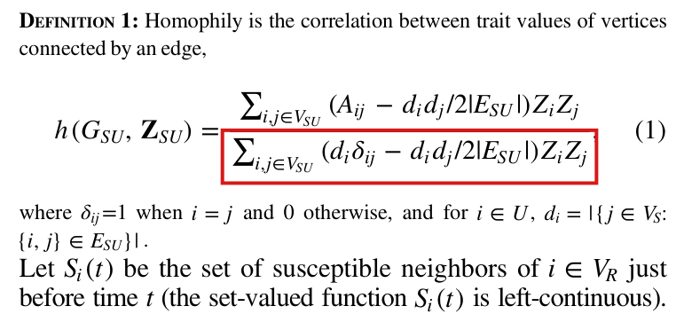
(S4) Homophily. Section "Homophily and Preferential Recruitment", p. 155 (PDF p. 3): "Consider an RDS sample of size $n$ with recruitment graph $G_R = (V_R, E_R)$, degrees $\mathbf{d}_R$, and univariate binary traits $\mathbf{Z}_R$. Let $G_{SU} = (V_{SU}, E_{SU})$ be the augmented subgraph for this sample, with traits $\mathbf{Z}_{SU}$. The observed traits $\mathbf{Z}_R$ are a subset of $\mathbf{Z}_{SU}$. Let $\mathbf{A} = \{A_{ij}\}$ be the adjacency matrix of $G_{SU}$. A standard definition of network homophily is the correlation between edges and trait values, known as the assortativity coefficient (43–45). DEFINITION 1: Homophily is the correlation between trait values of vertices connected by an edge, $$h(G_{SU}, \mathbf{Z}_{SU}) = \frac{\sum_{i,j \in V_{SU}} (A_{ij} - d_i d_j/2|E_{SU}|) Z_i Z_j}{\sum_{i,j \in V_{SU}} (d_i \delta_{ij} - d_i d_j/2|E_{SU}|) Z_i Z_j}, \quad (1)$$ where $\delta_{ij}=1$ when $i = j$ and 0 otherwise, and for $i \in U$, $d_i = |\{j \in V_S : \{i, j\} \in E_{SU}\}|$."
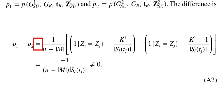
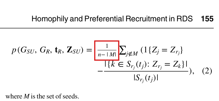
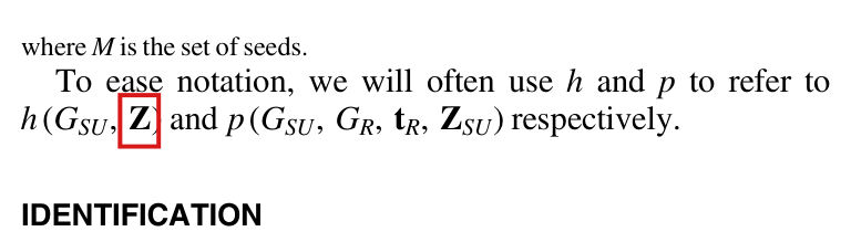
(S5) Preferential recruitment. p. 155 (PDF p. 3): "Let $S_i(t)$ be the set of susceptible neighbors of $i \in V_R$ just before time $t$ (the set-valued function $S_i(t)$ is left-continuous). Let $r_j$ be the recruiter of the sampled vertex $j \in V_S$. Under proportional (unbiased) recruitment, the probability of a recruiter recruiting a susceptible neighbor with the same trait value is proportional to the number of its susceptible neighbors with the same trait, $|\{k \in S_{r_j}(t_j) : Z_{r_j} = Z_k\}|$. In other words, recruitment is uniformly at random among susceptible neighbors. DEFINITION 2: Preferential recruitment is the average deviation from proportional recruitment, given knowledge of $G_{SU}$, $G_R$, $\mathbf{t}_R$, and $\mathbf{Z}_{SU}$, $$p(G_{SU}, G_R, \mathbf{t}_R, \mathbf{Z}_{SU}) = \frac{1}{n - |M|} \sum_{j \notin M} \left( 1\{Z_j = Z_{r_j}\} - \frac{|\{k \in S_{r_j}(t_j) : Z_{r_j} = Z_k\}|}{|S_{r_j}(t_j)|} \right), \quad (2)$$ where $M$ is the set of seeds. To ease notation, we will often use $h$ and $p$ to refer to $h(G_{SU}, \mathbf{Z})$ and $p(G_{SU}, G_R, \mathbf{t}_R, \mathbf{Z}_{SU})$ respectively." (The bare $\mathbf{Z}$ in the last sentence is as printed; see P012-T18.)
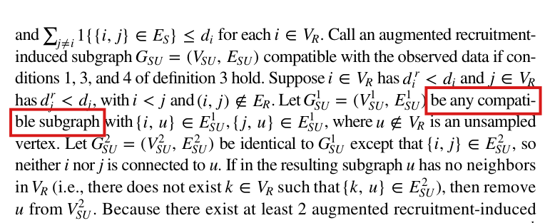
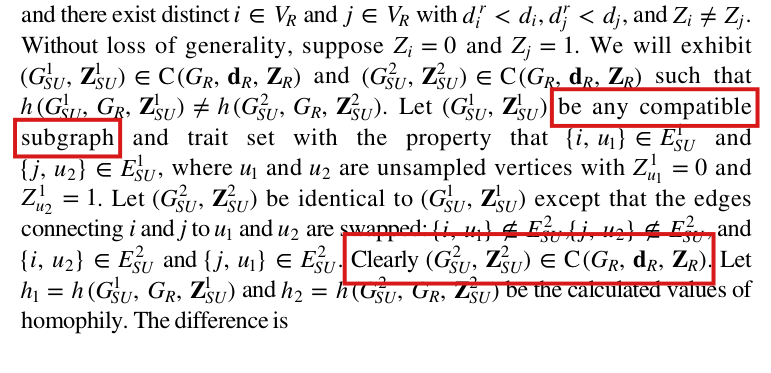
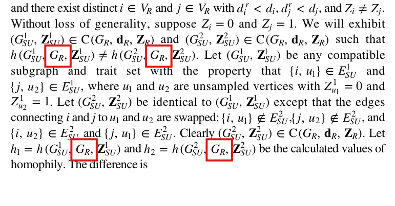
(S6) Compatibility. Section "Identification", p. 155 (PDF p. 3): "DEFINITION 3: Compatibility: The pair $(G_{SU}, \mathbf{Z}_{SU})$ is compatible with the observed data $G_R$, $\mathbf{d}_R$, and $\mathbf{Z}_R$ if 1) the recruitment graph is preserved ($G_R \subseteq G_{SU}$); 2) the set of recruited subjects' trait values is preserved ($\mathbf{Z}_R \subseteq \mathbf{Z}_{SU}$); 3) all unsampled vertices are connected to a recruited vertex (every $u \in V_{SU}$ with $u \notin V_S$ has an edge $\{v, u\}$ such that $v \in V_S$); and 4) total degree is preserved (for every $i \in V_R$, $d_i = \sum_{j \in V_{SU}} 1\{\{i, j\} \in E_{SU}\}$). Let $\mathrm{C}(G_R, \mathbf{d}_R, \mathbf{Z}_R)$ be the set of pairs $(G_{SU}, \mathbf{Z}_{SU})$ compatible with the observed data in the sense of definition 3 (this is a finite set). First, we examine whether $G_S$ and $G_{SU}$ are revealed by the observed data in RDS. Let $d_i^r$ be the degree of subject $i$ in the recruitment subgraph $G_R$."
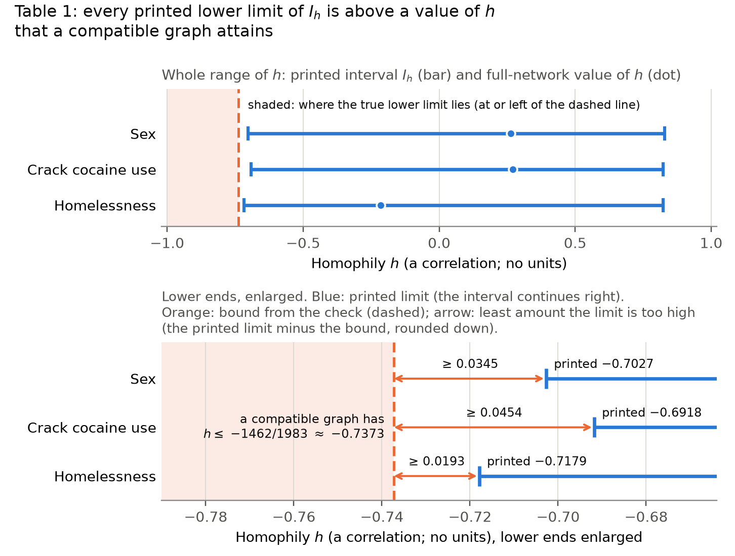
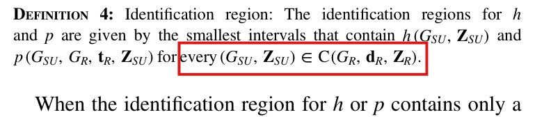
(S7) Identification region. p. 155 (PDF p. 3): "DEFINITION 4: Identification region: The identification regions for $h$ and $p$ are given by the smallest intervals that contain $h(G_{SU}, \mathbf{Z}_{SU})$ and $p(G_{SU}, G_R, \mathbf{t}_R, \mathbf{Z}_{SU})$ for every $(G_{SU}, \mathbf{Z}_{SU}) \in \mathrm{C}(G_R, \mathbf{d}_R, \mathbf{Z}_R)$. When the identification region for $h$ or $p$ contains only a single point, that parameter is point identified. Figure 1 shows an example of the identification regions."
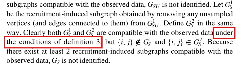
(S8) Readings used in every check of this audit and in every target below (they are not printed; with them the values printed in the paper's own Figure 1 are reproduced exactly). (R1) In (1) and (A1), $d_i d_j/2|E_{SU}|$ means $d_i d_j/(2|E_{SU}|)$ (the assortativity coefficient of references 43–45), and the sums run over ordered pairs $(i, j) \in V_{SU} \times V_{SU}$. For $i \in V_R$ the degree $d_i$ in $G$ equals the degree of $i$ in $G_{SU}$ (every edge of $G$ at a sampled vertex is in $E_S \cup E_U$), so in (1) every $d_i$, $i \in V_{SU}$, is the degree of $i$ in $G_{SU}$ and $\sum_{i \in V_{SU}} d_i = 2|E_{SU}|$. (R2) $G_R \subseteq G_{SU}$ in Definition 3 means $V_R \subseteq V_{SU}$ and $\{i, j\} \in E_{SU}$ for every directed edge $(i, j) \in E_R$; "$\{i, j\} \in E_R$" (Appendix, Web Appendix 2) means that $(i, j)$ or $(j, i)$ is in $E_R$; $d_i^r$ is the number of recruitment edges at $i$ in either direction (its recruiter, if any, plus its recruits). An element of $\mathcal{C}$ is a simple undirected graph on $V_R \cup U$ in which every edge has at least one endpoint in $V_R$ ((S3): $E_{SU} = E_S \cup E_U$), together with binary traits on $V_{SU}$ extending $\mathbf{Z}_R$, satisfying conditions 1–4; elements that differ only by renaming unsampled vertices are identified (the sense in which $\mathcal{C}$ is finite); the number of unsampled vertices and their degrees are not otherwise restricted, and no population size is observed. (R3) Admissible observed data: every non-seed $j \in V_R \setminus M$ has exactly one recruiter $r_j \in V_R$, with $t_{r_j} < t_j$, seeds have none, so $E_R = \{(r_j, j) : j \in V_R \setminus M\}$ and $|E_R| = n - |M|$; the recruitment times are distinct; and $d_i \geq d_i^r$ for every $i \in V_R$, which holds exactly when $\mathcal{C} \neq \emptyset$. (R4) For a pair in $\mathcal{C}$ and $j \notin M$, $S_{r_j}(t_j)$ is the set of neighbours $k$ of $r_j$ in $G_{SU}$ that are not yet in the study just before $t_j$: $k \in U$, or $k \in V_R$ with $t_k \geq t_j$. It contains $j$, so $|S_{r_j}(t_j)| \geq 1$. (R5) A graph is "not identified" when at least two graphs are compatible with the observed data (Appendix, p. 160: "Because there exist at least 2 augmented recruitment-induced subgraphs compatible with the observed data, $G_{SU}$ is not identified"); $h$ or $p$ is "not point identified" when it takes at least two values on $\mathcal{C}$ ((S7)).
(S9) Web Appendix 2 as printed, Web Appendix pp. 2–3 (the text and lines 1–2 are on p. 2, lines 3–27 and the rest on p. 3): "Suppose $(G_{SU}, \mathbf{Z}_{SU}) \in \mathcal{C}(G_R, \mathbf{d}_R, \mathbf{Z}_R)$ is a compatible augmented subgraph and trait set, and we wish to propose another compatible pair $(G^*_{SU}, \mathbf{Z}^*_{SU}) \in \mathcal{C}(G_R, \mathbf{d}_R, \mathbf{Z}_R)$. We outline two proposal mechanisms. The first removes or adds an edge in $G_{SU}$. If necessary, a new unsampled vertex $u$ is invented, and assigned a trait value $Z_u$. Let $U = \{u \in V_{SU} : u \notin V_R\}$ be the set of unsampled vertices. Furthermore, let $U_{-k} = \{u \in V_{SU} \setminus V_R : \{k, u\} \notin E_{SU}\}$ be the set of unsampled vertices in $U$ that are not connected to $k \in V_R$.
1: Let $G^*_{SU} = G_{SU}$ and $\mathbf{Z}^*_{SU} = \mathbf{Z}_{SU}$
2: Randomly choose $i \in V_R$ and $j \in V_{SU}$ with $i \neq j$.
3: if $\{i, j\} \in E_{SU}$ and $\{i, j\} \notin E_R$ then
4: Remove $\{i, j\}$ from $E^*_{SU}$
5: $B \sim \mathrm{Bernoulli}(1/2)$
6: if $B < 0.5$ and $U_{-i} \neq \emptyset$ then
7: Randomly choose $u \in U_{-i}$
8: else
9: Add a new vertex $u$ to $V^*_{SU}$
10: Randomly choose a trait $Z^*_u \in \{0, 1\}$
11: end if
12: Add $\{i, u\}$ to $E^*_{SU}$
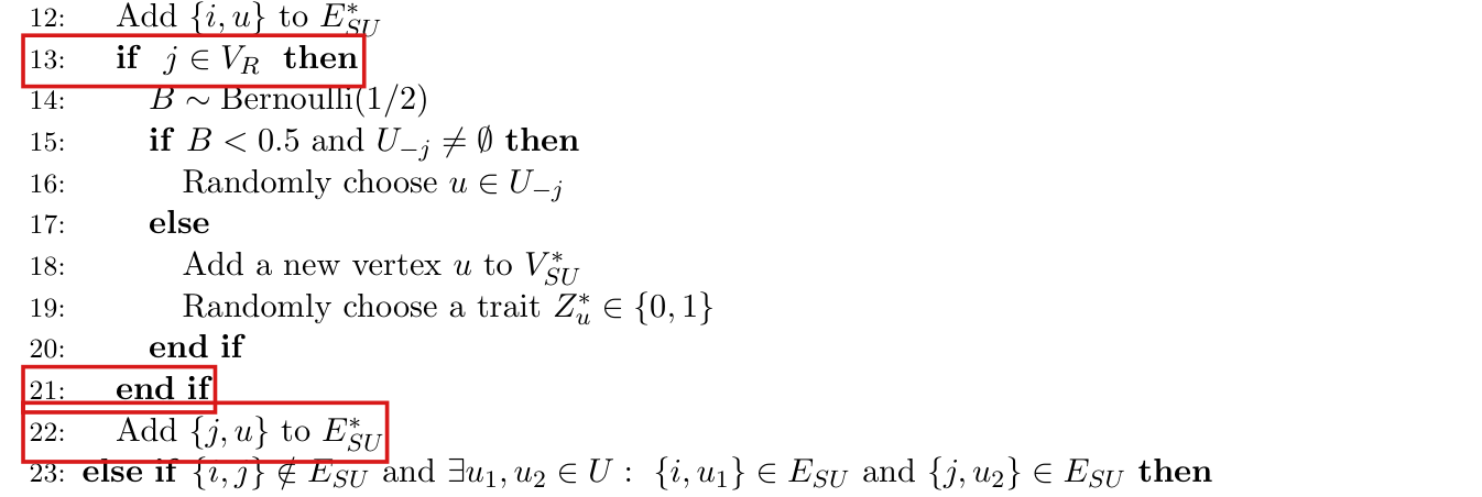
13: if $j \in V_R$ then
14: $B \sim \mathrm{Bernoulli}(1/2)$
15: if $B < 0.5$ and $U_{-j} \neq \emptyset$ then
16: Randomly choose $u \in U_{-j}$
17: else
18: Add a new vertex $u$ to $V^*_{SU}$
19: Randomly choose a trait $Z^*_u \in \{0, 1\}$
20: end if
21: end if
22: Add $\{j, u\}$ to $E^*_{SU}$
23: else if $\{i, j\} \notin E_{SU}$ and $\exists u_1, u_2 \in U : \{i, u_1\} \in E_{SU}$ and $\{j, u_2\} \in E_{SU}$ then
24: Remove $\{i, u_1\}$ and $\{j, u_2\}$ from $E^*_{SU}$
25: Add $\{i, j\}$ to $E^*_{SU}$
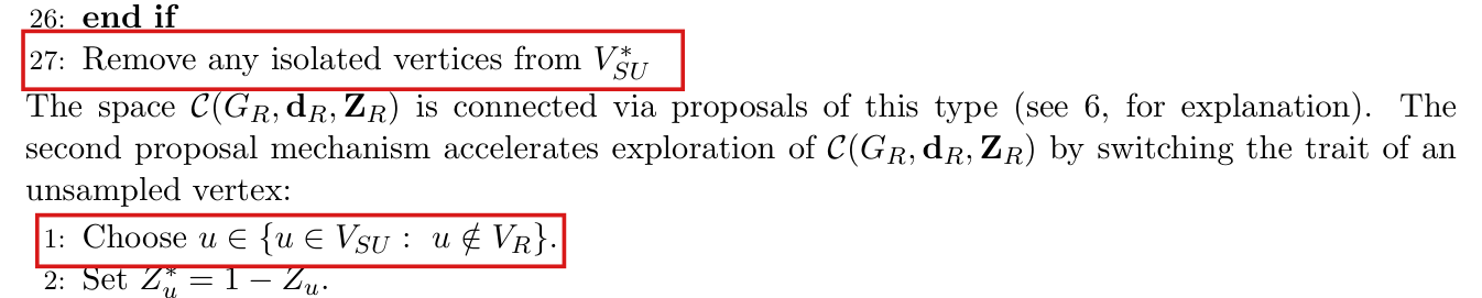
26: end if
27: Remove any isolated vertices from $V^*_{SU}$
The space $\mathcal{C}(G_R, \mathbf{d}_R, \mathbf{Z}_R)$ is connected via proposals of this type (see 6, for explanation). The second proposal mechanism accelerates exploration of $\mathcal{C}(G_R, \mathbf{d}_R, \mathbf{Z}_R)$ by switching the trait of an unsampled vertex:
1: Choose $u \in \{u \in V_{SU} : u \notin V_R\}$.
2: Set $Z^*_u = 1 - Z_u$.
Together, these proposal mechanisms result in a well-mixing sequence $(G_{SU}, \mathbf{Z}_{SU})_t$." In the printed listing lines 4–22 are indented under the `if` of line 3; lines 14–20 are indented under the `if` of line 13, which the `end if` of line 21 closes; line 22 is printed at the indentation of lines 12, 13 and 21, that is, inside the block of line 3 and outside the block of line 13. The listing is read as ordinary imperative pseudocode: starred objects are the proposal; $U$ and $U_{-k}$ are computed from the current $G_{SU}$; $u$ keeps the value last assigned to it; a "new vertex" is a vertex not in $V^*_{SU}$ when it is added.
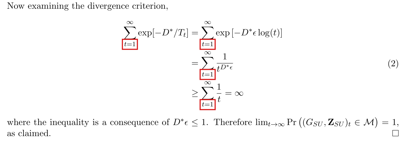
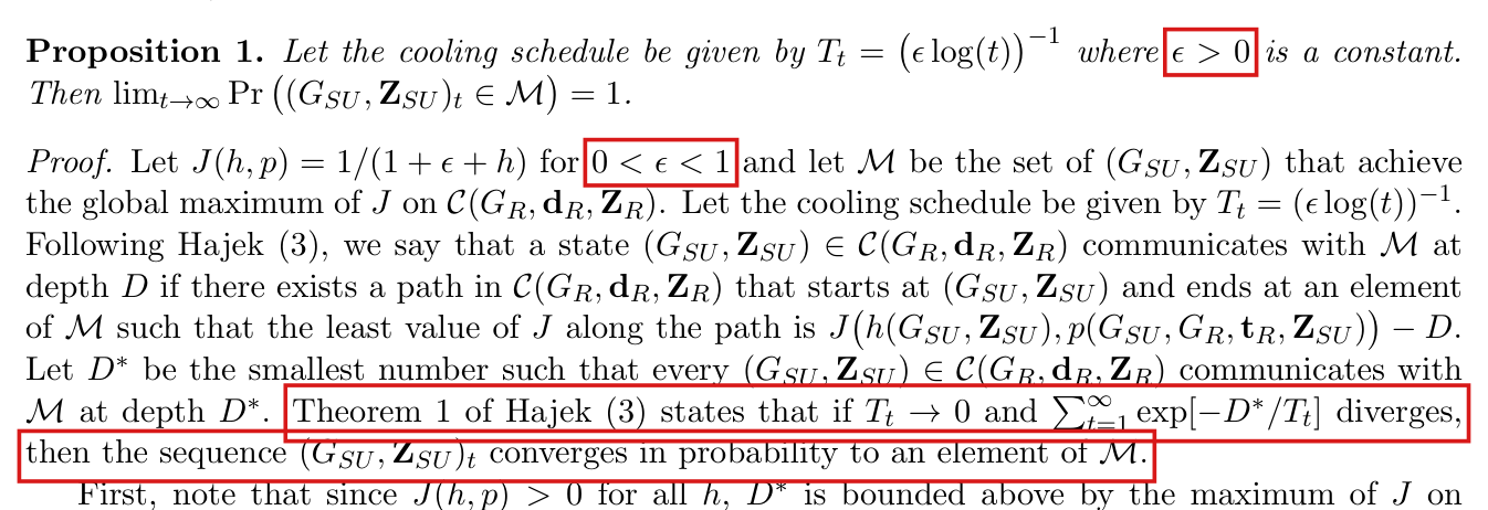
(S10) Web Appendix 1, set-up, Web Appendix p. 1, continuing on p. 2: "Let $J : [-1, 1]^2 \to \mathbb{R}$ be a function taking arguments $h(G_{SU}, \mathbf{Z}_{SU})$ and $p(G_{SU}, G_R, \mathbf{t}_R, \mathbf{Z}_{SU})$ for $(G_{SU}, \mathbf{Z}_{SU}) \in \mathcal{C}(G_R, \mathbf{d}_R, \mathbf{Z}_R)$. We choose this function, abbreviated $J(h, p)$, so that a desired feature of $\mathcal{C}(G_R, \mathbf{d}_R, \mathbf{Z}_R)$ coincides with the maximum of $J$. For example, the maximum of the function $$J(h, p) = \frac{1}{1 + \epsilon + h}$$ on $\mathcal{C}(G_R, \mathbf{d}_R, \mathbf{Z}_R)$ where $\epsilon > 0$, coincides with the lower identification bound of $h$. For concreteness in what follows, we will assume $J(h, p)$ has this form; similar definitions can be formulated individually to find the maximum of $h$, and the minimum and maximum of $p$. For $T > 0$, define the objective function $\pi(h, p) \propto \exp[J(h, p)/T]$. Our goal is to find $(G_{SU}, \mathbf{Z}_{SU}) \in \mathcal{C}(G_R, \mathbf{d}_R, \mathbf{Z}_R)$ such that $\pi\big(h(G_{SU}, \mathbf{Z}_{SU}), p(G_{SU}, G_R, \mathbf{t}_R, \mathbf{Z}_{SU})\big)$ is maximized. Let $$K\big((G_{SU}, \mathbf{Z}_{SU}), (G^*_{SU}, \mathbf{Z}^*_{SU})\big)$$ be a transition kernel that describes the probability of moving from a state $(G_{SU}, \mathbf{Z}_{SU}) \in \mathcal{C}(G_R, \mathbf{d}_R, \mathbf{Z}_R)$ to another state $(G^*_{SU}, \mathbf{Z}^*_{SU}) \in \mathcal{C}(G_R, \mathbf{d}_R, \mathbf{Z}_R)$. Let $T_t$ be a positive non-decreasing sequence indexed by $t$, with $\lim_{t \to \infty} T_t = 0$. We construct an inhomogeneous Markov chain on $\mathcal{C}(G_R, \mathbf{d}_R, \mathbf{Z}_R)$. At step $t$, where the current state is $(G_{SU}, \mathbf{Z}_{SU})$, we accept the proposed state $(G^*_{SU}, \mathbf{Z}^*_{SU}) \sim K\big((G_{SU}, \mathbf{Z}_{SU}), \cdot\big)$ with probability $$\rho_t = \min\left\{1, \exp\left[\frac{J\big(h(G^*_{SU}, \mathbf{Z}^*_{SU}), p(G^*_{SU}, G_R, \mathbf{t}_R, \mathbf{Z}^*_{SU})\big) - J\big(h(G_{SU}, \mathbf{Z}_{SU}), p(G_{SU}, G_R, \mathbf{t}_R, \mathbf{Z}_{SU})\big)}{T_t}\right]\right\}.$$ The proposal function is described formally below. As $T_t \to 0$, the samples $(G_{SU}, \mathbf{Z}_{SU})_t$ become more concentrated around local maxima of $\pi$. Convergence of the sequence $(G_{SU}, Z_{SU})_t$ to a global optimum depends on its ability to escape local maxima of $J$. The sequence $T_t$, called the "cooling schedule", controls the rate of convergence. Let $\mathcal{M}$ denote the set of $(G_{SU}, \mathbf{Z}_{SU}) \in \mathcal{C}(G_R, \mathbf{d}_R, \mathbf{Z}_R)$ for which $J\big(h(G_{SU}, \mathbf{Z}_{SU}), p(G_{SU}, G_R, \mathbf{t}_R, \mathbf{Z}_{SU})\big)$ is equal to the global maximum. Careful choice of $T_t$ ensures that the sequence of samples converges in probability to an element of $\mathcal{M}$."
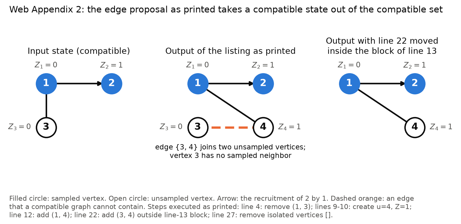
Effective claim (source TeX): [Printed statement refuted: Web Appendix 2, pp. 2–3] "Suppose $(G_{SU}, \mathbf{Z}_{SU}) \in \mathcal{C}(G_R, \mathbf{d}_R, \mathbf{Z}_R)$ is a compatible augmented subgraph and trait set, and we wish to propose another compatible pair $(G^*_{SU}, \mathbf{Z}^*_{SU}) \in \mathcal{C}(G_R, \mathbf{d}_R, \mathbf{Z}_R)$. We outline two proposal mechanisms." The first mechanism is the listing of lines 1–27 and the second the two-line trait flip, both transcribed in full in (S9) and in P012-T19; Web Appendix 1 takes them as "a transition kernel that describes the probability of moving from a state $(G_{SU}, \mathbf{Z}_{SU}) \in \mathcal{C}(G_R, \mathbf{d}_R, \mathbf{Z}_R)$ to another state $(G^*_{SU}, \mathbf{Z}^*_{SU}) \in \mathcal{C}(G_R, \mathbf{d}_R, \mathbf{Z}_R)$". [Counterexample, from the validators] (a) [Line 22 runs when $j$ is unsampled.] Observed data: $V_R = \{1, 2\}$, $E_R = \{(1, 2)\}$, $M = \{1\}$, $(t_1, t_2) = (1, 2)$, $\mathbf{d}_R = (2, 1)$, $\mathbf{Z}_R = (0, 1)$. Current state: $V_{SU} = \{1, 2, 3\}$, $E_{SU} = \{\{1, 2\}, \{1, 3\}\}$, $Z_3 = 0$. It is in $\mathcal{C}$: the recruitment edge is present, the sampled traits are $(0, 1)$, the unsampled vertex 3 has the sampled neighbour 1, the sampled degrees are $(2, 1)$, and no edge joins two unsampled vertices; at this state $h = -1/3$ and $p = -1/2$. Run the first mechanism with $i = 1$, $j = 3$. Line 3 holds ($\{1, 3\} \in E_{SU}$ and it is not a recruitment edge). Line 4 removes $\{1, 3\}$. $U = \{3\}$ and $U_{-1} = \emptyset$, so for either value of $B$ lines 9–10 add a new vertex $u = 4$ with a trait $Z^*_4 \in \{0, 1\}$. Line 12 adds $\{1, 4\}$. The condition of line 13 is false ($3 \notin V_R$), lines 14–20 are skipped, and $u$ is still 4. Line 22 adds $\{3, 4\}$. No vertex is isolated, so line 27 removes nothing. The output is $V^*_{SU} = \{1, 2, 3, 4\}$, $E^*_{SU} = \{\{1, 2\}, \{1, 4\}, \{3, 4\}\}$, $\mathbf{Z}^*_{SU} = (0, 1, 0, Z^*_4)$. For both values of $Z^*_4$ it is not in $\mathcal{C}$: the edge $\{3, 4\}$ joins two unsampled vertices, which $G_{SU}$ excludes ((S3)), and vertex 3 has no neighbour in $V_S$, contrary to condition 3 of Definition 3. Conditions 1, 2 and 4 still hold. Every execution with $(i, j) = (1, 3)$ ends in this way. (b) [A second instance.] $V_R = \{1, 2, 3\}$, $E_R = \{(1, 2), (2, 3)\}$, $M = \{1\}$, $(t_1, t_2, t_3) = (1, 2, 3)$, $\mathbf{d}_R = (1, 3, 1)$, $\mathbf{Z}_R = (0, 1, 0)$; current state $V_{SU} = \{1, 2, 3, 4\}$, $E_{SU} = \{\{1, 2\}, \{2, 3\}, \{2, 4\}\}$, $Z_4 = 0$, which is in $\mathcal{C}$. With $i = 2$, $j = 4$: $U_{-2} = \emptyset$, a new vertex 5 is added and joined to 2, line 13 is false, line 22 adds $\{4, 5\}$, line 27 removes nothing. Output edges $\{\{1, 2\}, \{2, 3\}, \{2, 5\}, \{4, 5\}\}$: $\{4, 5\}$ joins two unsampled vertices and vertex 4 has no sampled neighbour, for every value of $B$ and of $Z^*_5$. (c) [Line 27 can remove a sampled vertex.] $V_R = \{1, 2, 3\}$, $E_R = \{(1, 2)\}$, $M = \{1, 3\}$, $(t_1, t_2, t_3) = (1, 2, 3)$, $\mathbf{d}_R = (1, 1, 0)$, $\mathbf{Z}_R = (0, 1, 0)$; current state $V_{SU} = V_R$, $E_{SU} = \{\{1, 2\}\}$, which is in $\mathcal{C}$ (with $h = -1$, $p = 0$). With $i = 1$, $j = 2$: line 3 is false ($\{1, 2\}$ is a recruitment edge), line 23 is false ($\{1, 2\} \in E_{SU}$), and line 27 removes the isolated vertex 3, which is a sampled vertex. The output has $V^*_{SU} = \{1, 2\} \not\supseteq V_R$ and is not in $\mathcal{C}$ (conditions 1 and 2 of Definition 3 fail). (d) [The second mechanism has nothing to choose when no vertex is unsampled.] $V_R = \{1, 2\}$, $E_R = \{(1, 2)\}$, $M = \{1\}$, $\mathbf{d}_R = (1, 1)$, $\mathbf{Z}_R = (0, 1)$; the state $V_{SU} = V_R$, $E_{SU} = \{\{1, 2\}\}$ is in $\mathcal{C}$ (it is its only element), and $\{u \in V_{SU} : u \notin V_R\} = \emptyset$, so line 1 of the second mechanism has no value.
: SAP.P012a.T1WholeStatement
Theorem: SAP.P012a.T1
Statement hash: a9f4640f5ed56f163431422c8eff455e689c32b4d39322df0e9a6a6f4ce900f4
Statement definition: SAP.P012a.T1WholeStatement
Certificate. 20261104T181100Z
Declaration review: faithful; 2026-11-04T18:47:52Z; binding v2
Evidence scope: Certification checks formal proof objects. Statement fidelity is a model judgment. Author review is separate.
Proof dependencies: Independently extracted
Source and evidence metadata · sap-2026-11-08-assured-release




My comment and the history of this entry