LLM-generated corrections to the published research of P. M. Aronow

Journal article P013

Corrections to: Estimating Average Causal Effects Under General Interference, with Application to a Social Network Experiment

P. M. Aronow and Cyrus Samii (2017). Estimating Average Causal Effects Under General Interference, with Application to a Social Network Experiment. Annals of Applied Statistics 11(4):1912–1947.

DOI
10.1214/16-aoas1005
arXiv
1305.6156
Audited edition
Annals of Applied Statistics, 2017, 11(4):1912–1947; 36 pages in the audited file
SHA-256 of the audited file
2e01576f8c944e7ec8fdcec991101c7a1fd1f03c2cab60799ddbef3951dbf233
Replication materials
P013-E008, P013-E013, P013-N013, P013-N015, P013-N016, P013-N020
Permanent address
https://pmaronow.github.io/llm-audit/works/P013/

Summary

The paper asks how to estimate average causal effects in a randomized experiment when one unit’s treatment can affect another’s outcome. It gives Horvitz–Thompson estimators with conservative variance estimators and asymptotic results, a simulation and a field application. 21 entries are classified as errors (4 Moderate, 17 Minor) in the article and related software, and 7 are clarity notes; 9 further concerns were not confirmed, 4 remain unresolved and 1 is outside the scope. Under the intended dependence condition, Proposition 6.2 on interval coverage can be repaired by adding a uniform positive lower bound on positive joint exposure probabilities used by its variance estimator (P013-E001); this bound holds for the simulation and application designs under the stated regularity conditions.

What was and was not checked

I read the article in full, the source of the later R package interference (version 0.1.0, credited to Stephanie Zonszein, Cyrus Samii and P. M. Aronow) and a third party’s replication study. For the application of Section 10, I also read the materials of the field experiment. I read its eleven analysis scripts in full against Section 10 and Table 2. I used the public data release (ICPSR study 37070, version 2), and I read the entries of its codebook and questionnaire on the design, the nominations and the wristband. I checked the following and found them correct, with the qualifications stated.

  • Section 3: the matrix identities for the exposure probabilities; Proposition 3.1 for replicates drawn independently; the identity E[(R+1)/(Xi+1)]=(1−(1−πi(dk))R+1)/πi(dk)\mathrm{E}[(R+1)/(X_i+1)]=(1-(1-\pi_i(d_k))^{R+1})/\pi_i(d_k) used in Appendix A.3; and the printed example of 10,593 replicates.
  • Lemma 4.1 and Proposition 4.2, with equations (2) and (4)–(6), by derivation and by exact enumeration of small designs with interference and outcomes of mixed sign.
  • Propositions 5.1–5.6 and Appendix A.5: the bias of the variance estimators, the corrections based on Young’s inequality, their direction and their cases of equality, and the conservativeness in expectation of equation (11), for signed outcomes and with joint exposure probabilities equal to zero.
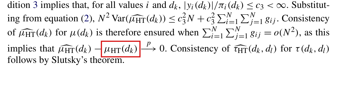
  • Proposition 6.1 and Appendix A.6: the variance bound and consistency under Conditions 3 and 4, apart from the subscript corrected in P013-E012.
  • Appendix A.7: I checked the covariance count after adding self-edges to the dependency graph, and the central limit theorem for the point estimator, for a dependency graph of bounded degree. The coverage statement is the subject of P013-E001, P013-E007 and P013-E011.
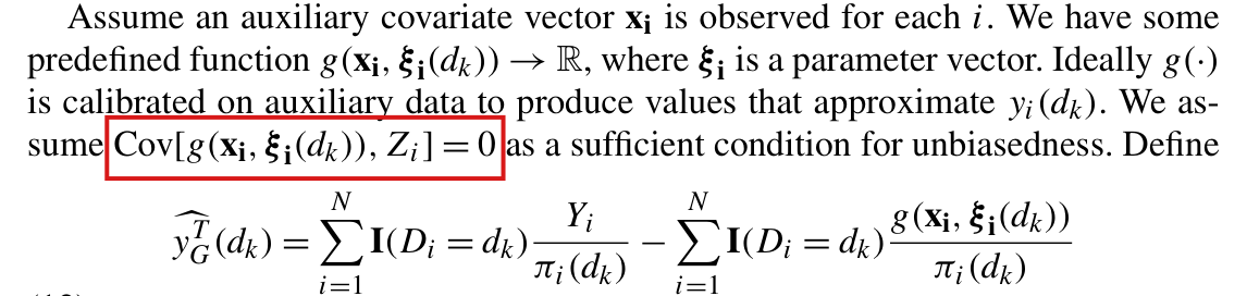
  • Section 7: equations (12) and (13) are unbiased for fixed predictions and agree with each other, and the bound on the bias of the Hajek estimator on p. 1929 follows when the ratio is defined.
  • Proposition 8.1, Corollary 8.1 and Appendix A.8.
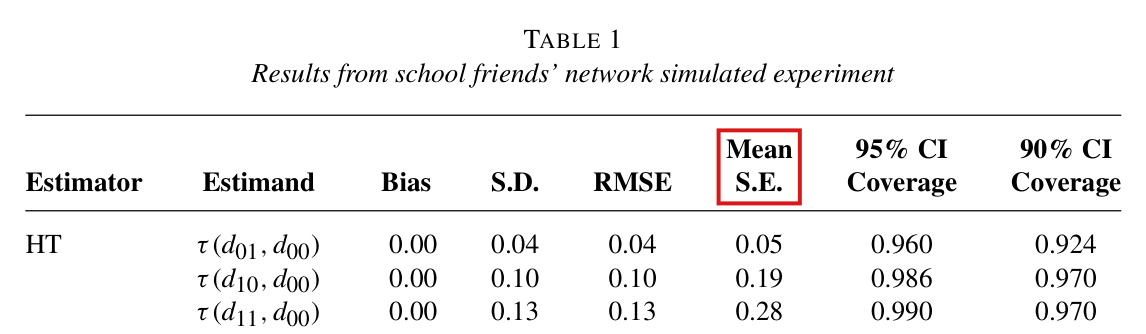
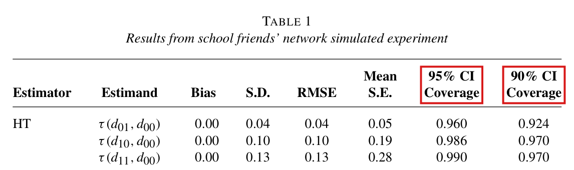
  • Table 1: the root mean squared error equals bias2+SD2\sqrt{\text{bias}^2+\text{SD}^2} within rounding in all 15 rows, the coverage entries are possible with 500 replications, and the statements of the text agree with the table.
  • The exposure mappings of Sections 9 and 10 partition the assignments as stated.
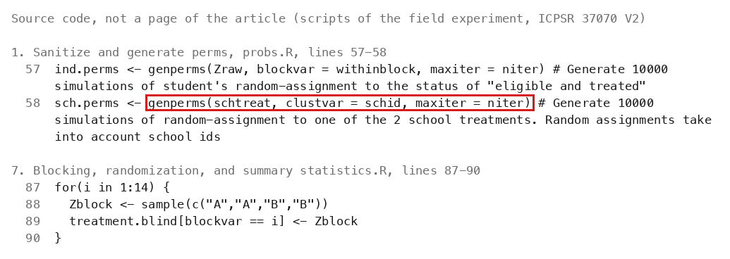
  • Section 10, the design: the script that assigned the schools and the public data show 56 schools in 14 blocks of four, with two host schools in each block. Every school has between 40 and 64 eligible students (2,943 in all). In the host schools, half of the eligible students are assigned to participate (728 of 1,456), within four student blocks per school. The script that simulates the assignments omits the school blocks (P013-N016).
  • Section 10, the network and the exposures: the released script builds an undirected graph within each school from the ten nominations of the first-wave survey, with a tie if either student named the other. Its five exposure indicators are the five conditions of the article. The recall period of the nomination question is the subject of P013-N015.
  • Section 10, the mean of 0.000 in the no-exposure condition: on the public data, none of the 1,487 eligible students of the control schools is coded as wearing the orange wristband.
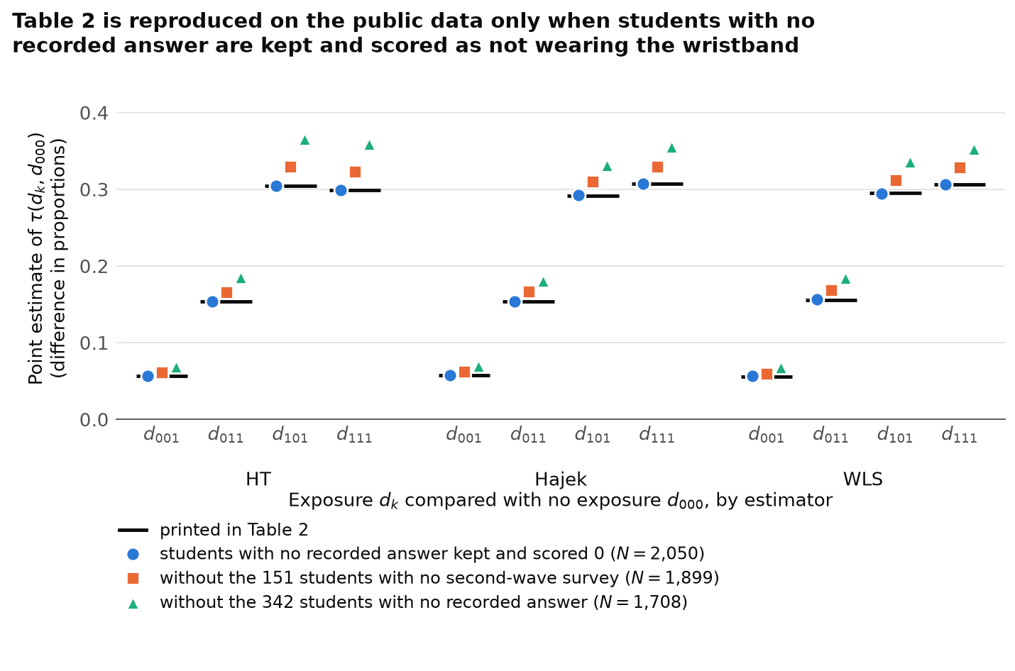
  • Table 2, the point estimates: all twelve are reconstructed on the public data to three decimals, with N=2,050N=2{,}050, using 10,000 probability draws with seed 123 and the pre-R-3.6 sampler, under four conditions. The eligible students are kept if their five simulated exposure probabilities exceed 0.010.01, which is not the rule that the article states. The outcome is the orange-wristband indicator with absent answers counted as zero (P013-N020). The weights are inverse exposure probabilities (P013-E013). The reconstructed WLS fit has one slope on network degree for all exposures.
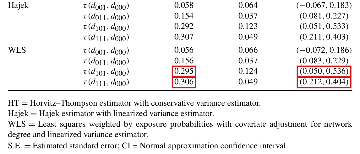
  • Table 2, the intervals: the four HT intervals, the four Hajek intervals and the WLS interval for d011d_{011} equal the estimate ±1.96\pm1.96 standard errors within rounding, and the magnitudes quoted in the text agree with the table. The WLS rows for d101d_{101} and d111d_{111} are the subject of P013-E008.
  • Section 10, the naive comparison of p. 1937: in the reconstructed sample on the public data, the contrast of participants with eligible nonparticipants in program schools is 0.1590.159, against 0.2880.288 for participants and students with no exposure.
  • In the R package interference, the point estimators, equations (7), (10) and (11), the correction for zero joint probabilities and the two estimators of the exposure probabilities agree with the formulas of the paper, apart from P013-E018, P013-N012 and P013-N013.

My checks had the following limits. The Add Health outcome and network files that the simulation reads were not available. Table 1, Figure 3 and the exposure probabilities quoted in Section 9 were therefore not reproduced. I did not run the simulation again, and I did not check the distributions of Appendix B numerically. None of the eleven scripts of the field experiment computes Table 2, and the script that did so was not available; the authors' own analysis files were not available to me. The scripts could not be run as written, because the input files that they name are not in the release. Their steps were applied to the public data through an adapter. Every recalculated value for Section 10 comes from the public data, which ICPSR’s notes say differ from the authors' files in some variables. I cannot establish that these are the values the authors' files would give. On the public data, the rule that the article states for the sample gives 2,196 students and not 2,050, and whether the published analysis used a cut-off is undetermined. The twelve standard errors of Table 2 were not reproduced. With the variance expressions of the article and with exact or simulated joint probabilities, no recalculated standard error rounds to its printed value, and the cause is not identified. The code that produced the published tables was not available, and the package is a later implementation whose link to those tables is not established. The functions of the package for two-stage designs were read for context, without checking them against their separate paper; its generated documentation and most of the codebook of the field experiment were read in part or not at all. The companion paper on the field experiment and most works cited by the article were not consulted; selected cited results on location invariance and dependency graphs were checked.

I stated selected results of the paper in Lean 4 with Mathlib as 27 targets with 255 statements. They cover the results of Sections 3 to 8, the corrected statements, the counterexamples to the printed ones, and the two findings on printed numbers P013-N004 and P013-E008. For the application of Section 10, they also cover the mathematical content of P013-N016 and P013-N020. The statements for P013-N016 give the exact probabilities that one school and that two schools host the program, under the block randomization that the article states and under the lottery that the released script simulates. They include an example of what the joint probabilities of that lottery do to the variance estimator of expression (7). The statements for P013-N020 say what the Horvitz–Thompson estimates measure when a student with no recorded answer is scored as not wearing, and by what factor each contrast changes when such students are removed from the sums. They include a two-unit example in which the recorded data do not determine the effect on wearing, and the printed description of the outcome read with Condition 2 for the wearing outcome of every student analysed. Of these statements, 242 are proved and 13 are counterexamples that are proved. The proofs include the counterexamples to Proposition 6.2 and to the convergence claims of Appendix A.7, the corrected Proposition 6.2 and its two bounds on the variance of the variance estimator, and the corrected statements for Appendix A.7. They also refute Proposition 4.1, its rule for the number of replicates and Proposition 6.2 as printed, as in P013-E003 and P013-E001. The counts 2,050, 342 and 151 come from the reconstruction on the public data, and two statements take them as given numbers or as hypotheses. The Lean statements do not verify these counts or any other empirical input, and they do not reproduce an entry of Table 2. The absence of further corrections does not establish that the rest of the paper is correct.

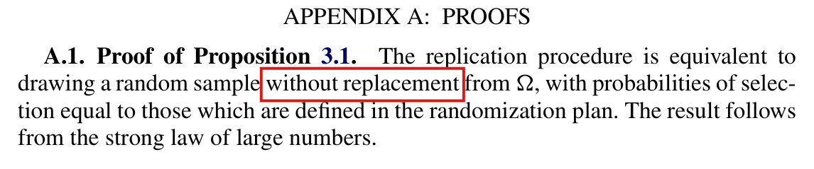
The rejection of repeated Bernoulli vectors occurs in that later package (P013-N012); I have not established that it was used for the published calculations. Appendix A.1’s separate without-replacement wording needs the clarification in P013-E010.

Headline claims and related corrections

  1. For a randomized experiment with interference of arbitrary but known form (a known design plus a correctly specified exposure mapping), the inverse-probability-weighted (Horvitz-Thompson) estimators of exposure-specific totals, means and average unit-level causal effects are unbiased, with the stated randomization variance and covariance.

    Lemma 4.1; Proposition 4.2; equations (1)-(6)

    See P013-E003, P013-E018, P013-N012.

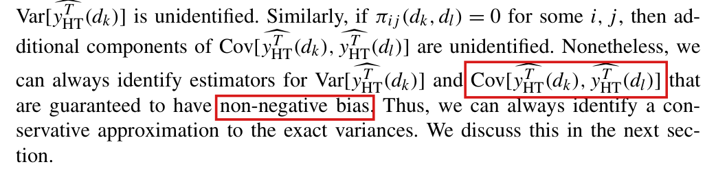
  2. The proposed randomization-based variance estimators are conservative (non-negatively biased for the variance of the estimated effect), including when exposures are clustered and some joint exposure probabilities are zero, and the covariance estimator is unbiased when the two exposures have identical potential outcomes.

    Lemma 5.1; Propositions 5.1-5.6; expressions (7)-(11); Appendix A.5 (Propositions A.1, A.2, Corollaries A.1, A.2)

    See P013-E009, P013-N001.

  3. Under bounded outcomes and bounded inverse marginal exposure probabilities and a vanishing fraction of pairwise exposure dependencies, the HT estimator of the average effect is consistent.

    Proposition 6.1; Conditions 3-4; Appendix A.6

    See P013-E012.

  4. Under local dependence and a positive limiting scaled variance, the effect estimator is asymptotically normal and Wald intervals built from the conservative variance estimator cover at least at the nominal rate for large NN.

    Proposition 6.2; Conditions 3, 5-6; Appendix A.7

    See P013-E001, P013-E002, P013-E006, P013-E007, P013-E011, P013-E012.

  5. Efficiency can be improved at little cost through covariate adjustment (difference and regression estimators) and Hajek ratio estimation; the difference estimator stays unbiased, and the bias of the Hajek estimator is bounded and vanishes asymptotically.

    Section 7; equations (12)-(15); bias bound on p. 1929; Table 1

    See P013-E004, P013-E005.

  6. In a naturalistic simulation on Add Health school networks, the HT, Hajek and WLS estimators show no perceivable bias and have conservative standard errors with coverage above nominal, while OLS and difference-in-sample-means are biased and undercover.

    Table 1; Figures 1 and 3; Section 9; Appendix B

    See P013-N004, P013-E013, P013-E016, P013-E017, P013-E018, P013-E019, P013-N006.

  7. In the anti-conflict field experiment, direct exposure raises the probability of wearing a program wristband by about 30 percentage points and indirect (peer) exposure by about 15 to 16 points, while being in a program school without direct or indirect exposure has a small effect that is statistically indistinguishable from zero.

    Table 2; Figure 2; Section 10

    See P013-E008, P013-E014, P013-E013, P013-N016, P013-N020.

  8. If the exposure mapping is misspecified, the HT estimator is unbiased for a design-weighted average of randomization potential outcomes (the Hudgens-Halloran individual average potential outcome), so the effect estimate is a difference of such averages.

    Proposition 8.1; Corollary 8.1; Appendix A.8

    See P013-N003.

  9. When the set of assignments is too large to enumerate, exposure probabilities can be approximated by simulation with almost-sure convergence, and the relative bias of the resulting HT estimator is at most (1−π0)R+1(1-\pi_0)^{R+1}, which gives a rule for choosing the number of replicates RR.

    Proposition 3.1; Proposition 4.1; Appendix A.1, A.3

    See P013-E003, P013-E010, P013-N012.

  10. The field experiment had two levels of randomization: 28 of 56 schools were selected to host the program by block randomization; in every school 40 to 64 students were nonrandomly designated eligible, and in host schools half of the eligible students were block-randomized to participate. Peers are defined by an undirected graph built from first-wave nominations of up to 10 schoolmates, and school and student assignment induce five exposure conditions combining school, direct and indirect exposure.

    Section 10, design paragraph and exposure mapping; Figure 2; abstract and introduction in general terms

    See P013-E014, P013-N015, P013-N016.

  11. The program has substantial direct and indirect effects on willingness to endorse anti-conflict norms by wearing a program wristband; because of the indirect effects, comparing participants with nonparticipants inside program schools would drastically underestimate the program's effect, and ignoring indirect effects might understate the program's cost-effectiveness.

    Section 10, first paragraph of p. 1937; Table 2; motivation in the abstract and introduction

Corrections

Moderate (4)

A real substantive error with limited reach.

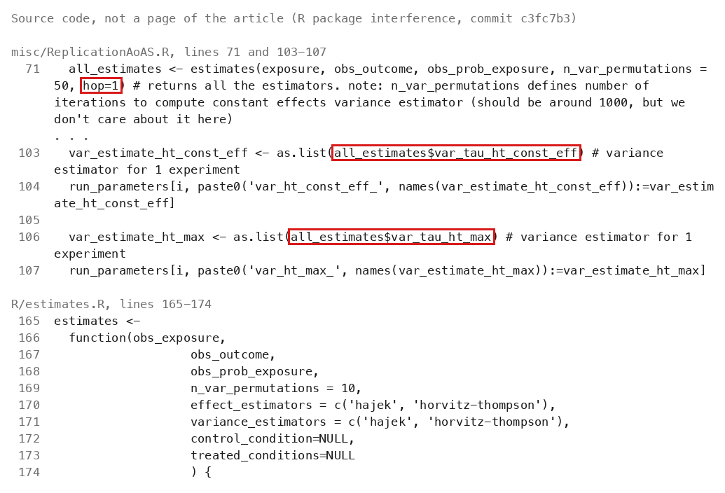
Proposition 6.2 needs a further condition, that the positive joint exposure probabilities that enter the variance estimator of equation (11) are bounded away from zero; Conditions 3, 5 and 6 alone do not imply the stated coverage.

Proposition 6.2, p. 1926 (PDF p. 15); Condition 3, p. 1925 (PDF p. 14); Appendix A.7, p. 1943 (PDF p. 32)

See also under Formal statements (Lean): P013-T1, P013-T2, P013-T18

My comment on this entry

As printed

Condition 3 (p. 1925): “Potential outcomes and exposure probabilities are bounded so that, for all values ii and dkd_k, ∣yi(dk)∣≤c1<∞|y_i(d_k)|\le c_1<\infty and ∣1/πi(dk)∣≤c2<∞|1/\pi_i(d_k)|\le c_2<\infty.”

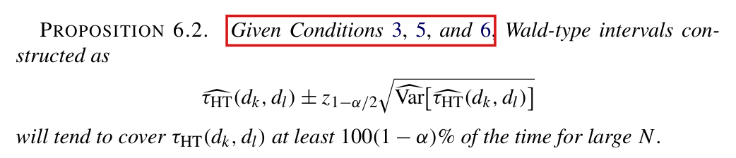
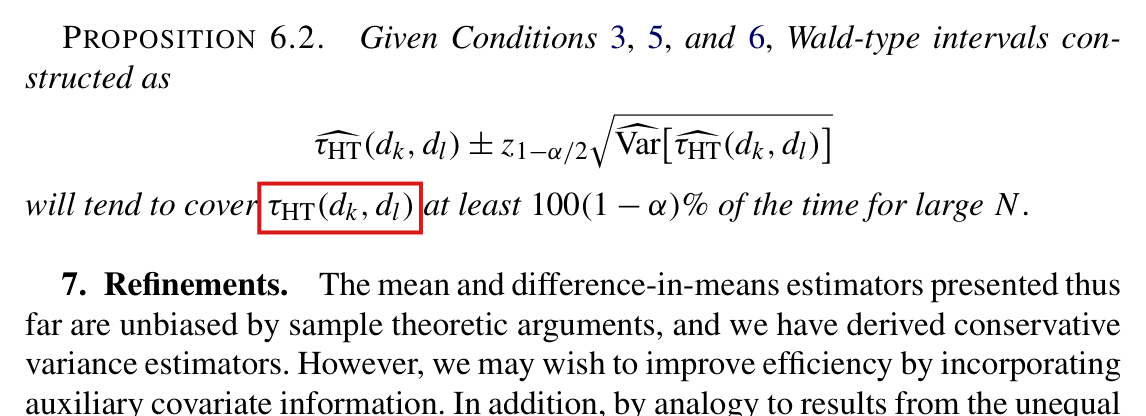
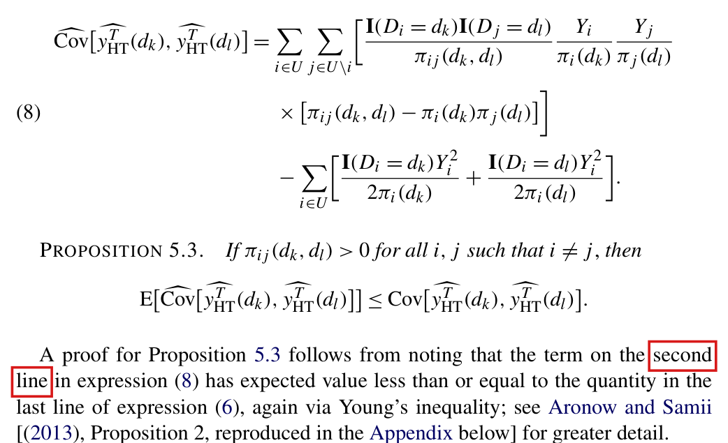
Proposition 6.2 (p. 1926): “Given Conditions 3, 5, and 6, Wald-type intervals constructed as

τ^HT(dk,dl)±z1−α/2Var⁡^[τ^HT(dk,dl)]\widehat{\tau}_{\mathrm{HT}}(d_k,d_l)\pm z_{1-\alpha/2}\sqrt{\widehat{\operatorname{Var}}[\widehat{\tau}_{\mathrm{HT}}(d_k,d_l)]}

will tend to cover τHT(dk,dl)\tau_{\mathrm{HT}}(d_k,d_l) at least 100(1−α)%100(1-\alpha)\% of the time for large NN.”

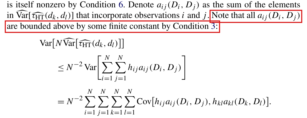
Appendix A.7 (p. 1943): “Denote aij(Di,Dj)a_{ij}(D_i,D_j) as the sum of the elements in Var⁡^[τ^HT(dk,dl)]\widehat{\operatorname{Var}}[\widehat{\tau}_{\mathrm{HT}}(d_k,d_l)] that incorporate observations ii and jj. Note that all aij(Di,Dj)a_{ij}(D_i,D_j) are bounded above by some finite constant by Condition 3:

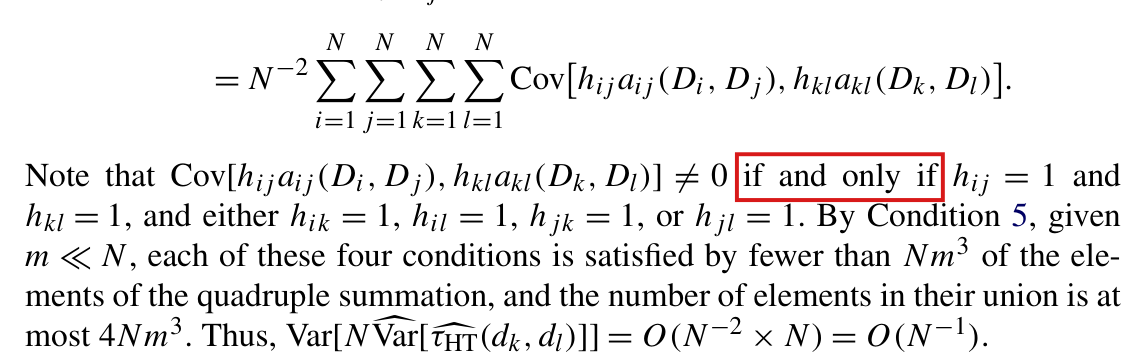
Var⁡[NVar⁡^[τ^HT(dk,dl)]]≤N−2Var⁡[∑i=1N∑j=1Nhijaij(Di,Dj)]=N−2∑i=1N∑j=1N∑k=1N∑l=1NCov⁡[hijaij(Di,Dj),hklakl(Dk,Dl)].\begin{aligned} \operatorname{Var}\bigl[N\widehat{\operatorname{Var}}[\widehat{\tau}_{\mathrm{HT}}(d_k,d_l)]\bigr] &\le N^{-2}\operatorname{Var}\Bigl[\sum_{i=1}^{N}\sum_{j=1}^{N}h_{ij}a_{ij}(D_i,D_j)\Bigr]\\ &=N^{-2}\sum_{i=1}^{N}\sum_{j=1}^{N}\sum_{k=1}^{N}\sum_{l=1}^{N}\operatorname{Cov}\bigl[h_{ij}a_{ij}(D_i,D_j),h_{kl}a_{kl}(D_k,D_l)\bigr]. \end{aligned}

… Thus, Var⁡[NVar⁡^[τ^HT(dk,dl)]]=O(N−2×N)=O(N−1)\operatorname{Var}[N\widehat{\operatorname{Var}}[\widehat{\tau}_{\mathrm{HT}}(d_k,d_l)]]=O(N^{-2}\times N)=O(N^{-1}).”

The problem

Proposition 6.2 states that, under Conditions 3, 5 and 6, Wald intervals built from the variance estimator of equation (11) are asymptotically conservative. Condition 3 bounds the potential outcomes and the inverse marginal exposure probabilities 1/πi(dk)1/\pi_i(d_k). Through equations (7) and (10), the variance estimator also divides by the positive joint exposure probabilities πij(dk)\pi_{ij}(d_k), πij(dl)\pi_{ij}(d_l) and πij(dk,dl)\pi_{ij}(d_k,d_l), and the three conditions do not keep these away from zero. The step of Appendix A.7 that takes every aij(Di,Dj)a_{ij}(D_i,D_j) to be bounded “by Condition 3” is therefore not justified. The bound O(N−1)O(N^{-1}) on the variance of the scaled variance estimator rests on that step, and it can fail. When it fails, the variance estimator can be unbiased and still converge in probability to a value below the true scaled variance, because the estimate is large on rare assignments. The interval then covers less often than its nominal level in the limit. This is so even when Condition 5 is read as a dependency graph of bounded degree, that is, after the correction of P013-E002.

Evidence an exact counterexample

The evidence is an exact counterexample to the printed statement and a derivation of the corrected one.

For N=2nN=2n, let the units form nn pairs that are randomized independently. Within a pair, the assignments (0,0)(0,0) and (1,1)(1,1) each have probability ϵn=1/(4n3)\epsilon_n=1/(4n^3), and (1,0)(1,0) and (0,1)(0,1) each have probability qn=1/2−ϵnq_n=1/2-\epsilon_n. There is no interference: Di=ZiD_i=Z_i, with dk=1d_k=1 and dl=0d_l=0. Both potential outcomes equal 11 for the first unit of each pair and −1-1 for the second, and the average effect is 00. The outcomes are bounded and every marginal exposure probability is 1/21/2, and Condition 3 holds with c1=1c_1=1 and c2=2c_2=2. Since the pairs are independent, Condition 5 holds with m=2m=2, for a genuine dependency graph. Further, I have NVar⁡[τ^HT]=8(1−2ϵn)→8N\operatorname{Var}[\widehat{\tau}_{\mathrm{HT}}]=8(1-2\epsilon_n)\to8, and Condition 6 holds. All joint exposure probabilities of distinct units are positive, and those of equal exposures within a pair equal ϵn→0\epsilon_n\to0.

Let V^N\widehat{V}_N denote the estimator of equation (11). Substituting into (7), (10) and (11), I obtain N2V^N=∑b=1nBbN^2\widehat{V}_N=\sum_{b=1}^{n}B_b, where Bb=2/ϵnB_b=2/\epsilon_n if the two units of pair bb receive the same assignment and Bb=16−2/qnB_b=16-2/q_n otherwise. Then E[Bb]=16(1−2ϵn)\mathrm{E}[B_b]=16(1-2\epsilon_n), and V^N\widehat{V}_N is exactly unbiased. The probability that some pair receives equal assignments is at most 2nϵn=1/(2n2)→02n\epsilon_n=1/(2n^2)\to0, and on the complementary event I have NV^N=8−1/qn→6N\widehat{V}_N=8-1/q_n\to6. I conclude that NV^N→6N\widehat{V}_N\to6 in probability, while NVar⁡[τ^HT]→8N\operatorname{Var}[\widehat{\tau}_{\mathrm{HT}}]\to8. Further, I find that

Var⁡[NV^N]=2(1−4ϵn)4nϵn(1−2ϵn)∼8n2,\operatorname{Var}[N\widehat{V}_N]=\frac{2(1-4\epsilon_n)^4}{n\epsilon_n(1-2\epsilon_n)}\sim8n^2,

contradicting the concentration bound in Appendix A.7. Since N τ^HT\sqrt{N}\,\widehat{\tau}_{\mathrm{HT}} is asymptotically normal with mean 00 and variance 88, the coverage of the nominal 100(1−α)%100(1-\alpha)\% interval tends to

2Φ(z1−α/23/4)−1<1−α,2\Phi\bigl(z_{1-\alpha/2}\sqrt{3/4}\bigr)-1<1-\alpha,

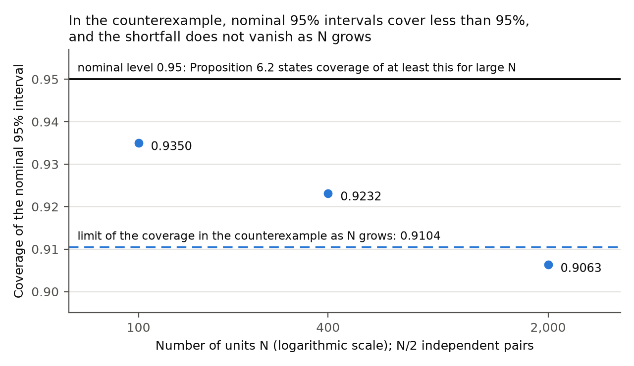
which is 0.91040.9104 for α=0.05\alpha=0.05. A variant of the example with ϵ=N−2\epsilon=N^{-2} has the same limits.

The counterexample at N=6N=6 (ϵ3=1/108\epsilon_3=1/108), by exact enumeration of all 64 assignments, and in the limit.
QuantityN=6N=6Limit
NVar⁡[τ^HT]N\operatorname{Var}[\widehat{\tau}_{\mathrm{HT}}]212/27≈7.85212/27\approx7.8588
E[NV^N]\mathrm{E}[N\widehat{V}_N]212/27≈7.85212/27\approx7.8588
NV^NN\widehat{V}_N when every pair is split316/53≈5.96316/53\approx5.9666
Probability that every pair is split148877/157464≈0.945148877/157464\approx0.94511

For the corrected statement, suppose in addition that every positive joint exposure probability that enters (7) and (10) is at least b>0b>0, and let Condition 5 hold for a symmetric dependency graph with row sums at most mm. I add every self-edge, writing h~ij=1\widetilde h_{ij}=1 when i=ji=j or hij=1h_{ij}=1. This preserves the dependency condition and bounds every row sum by m+1m+1. I write N2V^N=∑i,jBij(Di,Dj)N^2\widehat{V}_N=\sum_{i,j}B_{ij}(D_i,D_j), where BijB_{ij} collects the terms that involve units ii and jj. A term with positive joint probability is bounded in absolute value by (1+1/b)c12c22(1+1/b)c_1^2c_2^2, and the corrections for zero joint probabilities divide only by marginal probabilities. Then there exists a constant CC, which does not depend on the population size, such that ∣Bij∣≤C|B_{ij}|\le C for every pair of units. If h~ij=0\widetilde h_{ij}=0, then the exposures of ii and jj are independent, the joint probabilities are products of marginal probabilities, and Bij=0B_{ij}=0. Then at most N(m+1)N(m+1) of the BijB_{ij} are nonzero. Two of them can be correlated only if a unit of one is adjacent under h~\widetilde h to a unit of the other, which leaves at most 4N(m+1)34N(m+1)^3 nonzero covariances, each at most 4C24C^2 in absolute value. I obtain

Var⁡[NV^N]≤N−2 (4N(m+1)3)(4C2)=16C2(m+1)3/N→0.\operatorname{Var}[N\widehat{V}_N]\le N^{-2}\,(4N(m+1)^3)(4C^2)=16C^2(m+1)^3/N\to0.

Let cN=NVar⁡[τ^HT(dk,dl)]→c>0c_N=N\operatorname{Var}[\widehat{\tau}_{\mathrm{HT}}(d_k,d_l)]\to c>0. Proposition 5.6 implies that E[NV^N]≥cN\mathrm{E}[N\widehat{V}_N]\ge c_N. By Chebyshev’s inequality, I have P{NV^N<cN−δ}→0P\{N\widehat{V}_N<c_N-\delta\}\to0 for every δ>0\delta>0. The statistic TN=N(τ^HT(dk,dl)−τ(dk,dl))/cNT_N=\sqrt{N}(\widehat{\tau}_{\mathrm{HT}}(d_k,d_l)-\tau(d_k,d_l))/\sqrt{c_N} is asymptotically standard normal by the central limit theorem that Appendix A.7 invokes, which involves no joint probability. For 0<δ<c0<\delta<c, on the event NV^N≥cN−δN\widehat{V}_N\ge c_N-\delta the interval covers whenever ∣TN∣≤z1−α/21−δ/cN|T_N|\le z_{1-\alpha/2}\sqrt{1-\delta/c_N}. Then the lower limit of the coverage is at least 2Φ(z1−α/21−δ/c)−12\Phi(z_{1-\alpha/2}\sqrt{1-\delta/c})-1. Letting δ↓0\delta\downarrow0, I obtain the lower bound 1−α1-\alpha. The argument does not require that E[NV^N]\mathrm{E}[N\widehat{V}_N] converge.

The added condition holds automatically for the following designs described in the paper. Consider first Bernoulli assignment at a fixed rate pp with first-order interference on a graph of degree at most Δ\Delta, a fixed-rate version of the illustration given after Condition 5. A joint exposure event of two units is determined by at most 2(Δ+1)2(\Delta+1) independent assignments, and every positive joint probability is at least min⁡(p,1−p)2(Δ+1)\min(p,1-p)^{2(\Delta+1)}. In the design of Section 9, a fixed fraction of each school is treated uniformly and schools are randomized independently, and the bound follows from Condition 3. In the block-randomized design of Section 10, the blocks are randomized uniformly at fixed quotas and a school has at most 64 eligible students. Condition 3 then implies that every positive joint probability is at least c2−22−129c_2^{-2}2^{-129}. For arbitrary known designs the condition is a further restriction. The counterexample above, which has independent groups of two units, does not satisfy it.

What survives

The estimand, the Horvitz–Thompson point estimator and the variance estimator of equation (11) with its corrections for zero joint probabilities are unchanged. The results on unbiasedness in finite samples, the exact variance and covariance formulas and Proposition 5.6 are unaffected; in the counterexample Proposition 5.6 holds with equality. The point estimator is consistent and asymptotically normal under a dependency graph of bounded degree, and these properties do not involve joint probabilities. With the added condition the coverage conclusion holds, and the condition is automatic for the Bernoulli illustration with a fixed rate and for the designs of Sections 9 and 10 wherever Conditions 3 and 5 hold for them. No entry of Table 1 or Table 2 changes, and no reported interval is shown to undercover. What is lost is the claim for arbitrary known designs under Conditions 3, 5 and 6 alone; the refinements of Section 7, which use equation (11), need the same control in addition to their own assumptions. The example has limiting coverage 0.91040.9104, and it is not established that coverage can tend to zero.

Corrected

Proposition 6.2. Let Conditions 3 and 6 hold, and let Condition 5 hold with hijh_{ij} the indicator of a dependency graph, as corrected in P013-E002. Suppose in addition that there exists a constant b>0\colorbox{#ffe58a}{$b>0$}, not depending on N\colorbox{#ffe58a}{$N$}, that bounds from below every positive joint exposure probability entering equations (7) and (10): for all NN and all i≠ji\ne j, if πij(dk)>0\pi_{ij}(d_k)>0 then πij(dk)≥b\pi_{ij}(d_k)\ge b, and likewise for πij(dl)\pi_{ij}(d_l); and for all NN and all i,ji,j, if πij(dk,dl)>0\pi_{ij}(d_k,d_l)>0 then πij(dk,dl)≥b\pi_{ij}(d_k,d_l)\ge b. Joint probabilities equal to zero remain permitted, with the corrections of Section 5. Write V^N=Var⁡^[τ^HT(dk,dl)]\widehat{V}_N=\widehat{\operatorname{Var}}[\widehat{\tau}_{\mathrm{HT}}(d_k,d_l)] and V^N+=max⁡{0,V^N}\colorbox{#ffe58a}{$\widehat{V}_N^+=\max\{0,\widehat{V}_N\}$} to define the interval when the variance estimate is negative. Then the Wald-type intervals constructed as

τ^HT(dk,dl)±z1−α/2V^N+\widehat{\tau}_{\mathrm{HT}}(d_k,d_l)\pm z_{1-\alpha/2}\sqrt{\colorbox{#ffe58a}{$\displaystyle \widehat{V}_N^+$}}

satisfy

lim inf⁡N→∞ P{∣τ^HT(dk,dl)−τ(dk,dl)∣≤z1−α/2V^N+}≥1−α.\colorbox{#ffe58a}{$\displaystyle \liminf_{N\to\infty}$}\,P\Bigl\{\bigl|\widehat{\tau}_{\mathrm{HT}}(d_k,d_l)-\tau(d_k,d_l)\bigr|\le z_{1-\alpha/2}\sqrt{\colorbox{#ffe58a}{$\displaystyle \widehat{V}_N^+$}}\Bigr\}\ge1-\alpha .

The target is written τ(dk,dl)\tau(d_k,d_l), as in P013-E012.

The added condition may be replaced by the weaker one that, for every δ>0\delta>0,

P{NVar⁡^[τ^HT(dk,dl)]<NVar⁡[τ^HT(dk,dl)]−δ}→0.P\bigl\{N\widehat{\operatorname{Var}}[\widehat{\tau}_{\mathrm{HT}}(d_k,d_l)]<N\operatorname{Var}[\widehat{\tau}_{\mathrm{HT}}(d_k,d_l)]-\delta\bigr\}\to0 .

This holds if N(Var⁡^[τ^HT(dk,dl)]−E[Var⁡^[τ^HT(dk,dl)]])→0N(\widehat{\operatorname{Var}}[\widehat{\tau}_{\mathrm{HT}}(d_k,d_l)]-\mathrm{E}[\widehat{\operatorname{Var}}[\widehat{\tau}_{\mathrm{HT}}(d_k,d_l)]])\to0 in probability, and also if NbN→∞Nb_N\to\infty, where bNb_N is the smallest positive joint exposure probability entering (7) and (10) at size NN.

Appendix A.7: “Note that all aij(Di,Dj)a_{ij}(D_i,D_j) are bounded above by some finite constant by Condition 3 and the lower bound on the positive joint exposure probabilities.”

Crop of Proposition 6.2. A red box marks the words 'Given Conditions 3, 5, and 6'. The proposition continues: Wald-type intervals constructed as tau-hat-HT(d_k, d_l) plus or minus z_(1 minus alpha/2) times the square root of the estimated variance will tend to cover tau_HT(d_k, d_l) at least 100(1 minus alpha) percent of the time for large N.
Proposition 6.2, p. 1926 (PDF p. 15). The marked hypotheses do not suffice for the conclusion.
Crop of the middle of the proof of Proposition 6.2. Red boxes mark the sentence 'Note that all a_ij(D_i, D_j) are bounded above by some finite constant by Condition 3'. It is followed by a display bounding the variance of N times the estimated variance by N to the power minus 2 times a fourfold sum of covariances of the terms h_ij a_ij(D_i, D_j) and h_kl a_kl(D_k, D_l).
Appendix A.7, p. 1943 (PDF p. 32). The marked sentence takes the terms aij(Di,Dj)a_{ij}(D_i,D_j) of the variance estimator to be bounded by Condition 3, which bounds only the marginal exposure probabilities.
Chart with the number of units N on a logarithmic horizontal axis and the coverage of the nominal 95 percent interval on the vertical axis, with ticks from 0.90 to 0.95. Three blue points show midpoints of exact coverage brackets in the counterexample: 0.9350 at N = 100, 0.9232 at N = 400 and 0.9063 at N = 2,000. A solid black horizontal line at 0.95 is labelled as the nominal level that Proposition 6.2 states as a lower bound for large N. A dashed blue horizontal line at 0.9104 is labelled as the limit of the coverage in the counterexample as N grows. All three points lie below the solid line.
The counterexample for P013-E001: coverage of the nominal 95% interval of Proposition 6.2 for N=100N=100, 400400 and 2,0002{,}000 units (n=50n=50, 200200 and 1,0001{,}000 pairs, critical value 1.961.96), with the nominal level (solid line) and the limit 0.91040.9104 of the coverage (dashed line). Each point is the midpoint of an exact bracket of width below 0.00020.0002. The bounds use binomial probabilities and need not approach the limit monotonically.
My comment and the history of this entry

Agreed.

  1. Classification before my review (the classification when the audit was first completed, before I reviewed it): Moderate error.
  2. I commented.
  3. Independent evaluation. No change was needed: my comment agrees with the entry.

The bound of Proposition 4.1 holds for potential outcomes of one sign with nonzero total; for general nonzero totals, multiplying its right-hand side by ∑i∣yi(dk)∣/∣yT(dk)∣\sum_i|y_i(d_k)|/|y^T(d_k)| gives a valid bound, and the rule for the number of replicates changes in the same way.

Proposition 4.1 and the paragraph after it, p. 1920 (PDF p. 9); last inequality of Appendix A.3, p. 1938 (PDF p. 27)

See also under Formal statements (Lean): P013-T3, P013-T4, P013-T12

My comment on this entry

As printed

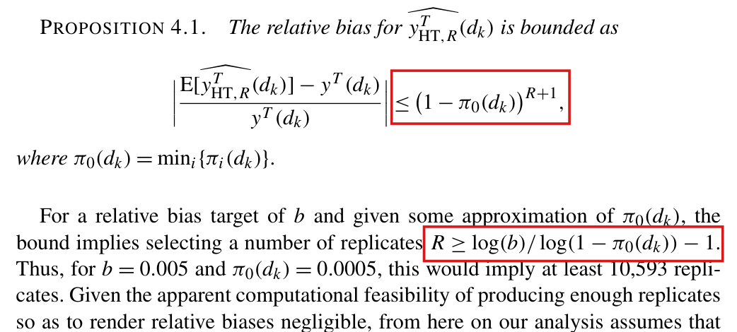
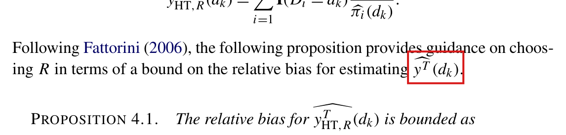
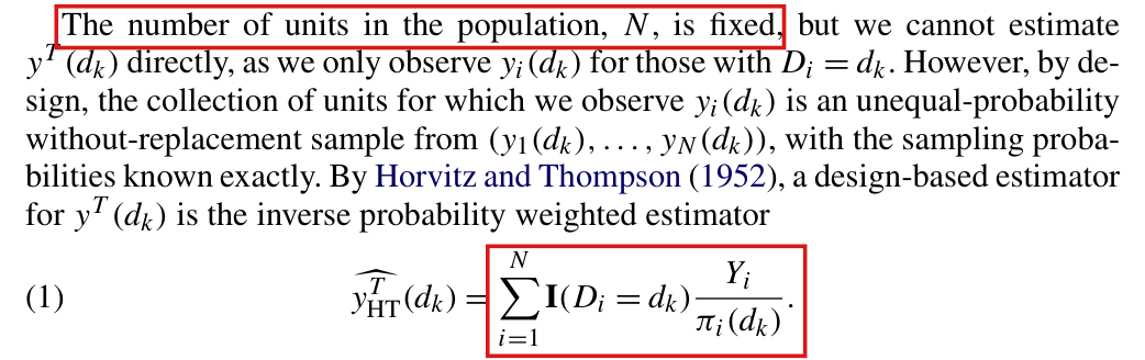
Proposition 4.1 (p. 1920): “The relative bias for yHT,RT^(dk)\widehat{y^T_{\mathrm{HT},R}}(d_k) is bounded as

∣E[yHT,RT^(dk)]−yT(dk)yT(dk)∣≤(1−π0(dk))R+1,\left|\frac{\mathrm{E}[\widehat{y^T_{\mathrm{HT},R}}(d_k)]-y^T(d_k)}{y^T(d_k)}\right|\le\colorbox{#ffe58a}{$\displaystyle (1-\pi_0(d_k))^{R+1}$},

where π0(dk)=min⁡i{πi(dk)}\pi_0(d_k)=\min_i\{\pi_i(d_k)\}.

For a relative bias target of bb and given some approximation of π0(dk)\pi_0(d_k), the bound implies selecting a number of replicates R≥log⁡(b)/log⁡(1−π0(dk))−1R\ge\log(\colorbox{#ffe58a}{$b$})/\log(1-\pi_0(d_k))-1. Thus, for b=0.005b=0.005 and π0(dk)=0.0005\pi_0(d_k)=0.0005, this would imply at least 10,593 replicates.”

Appendix A.3, last display (p. 1938):

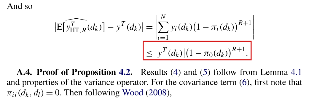
∣E[yHT,RT^(dk)]−yT(dk)∣=∣∑i=1Nyi(dk)(1−πi(dk))R+1∣≤∣yT(dk)∣(1−π0(dk))R+1.\left|\mathrm{E}[\widehat{y^T_{\mathrm{HT},R}}(d_k)]-y^T(d_k)\right|=\left|\sum_{i=1}^{N}y_i(d_k)(1-\pi_i(d_k))^{R+1}\right|\le\colorbox{#ffe58a}{$\displaystyle |y^T(d_k)|$}(1-\pi_0(d_k))^{R+1}.
The problem

Proposition 4.1 bounds the relative bias of the Horvitz–Thompson total computed with simulated exposure probabilities by (1−π0(dk))R+1(1-\pi_0(d_k))^{R+1}, and it places no restriction on the signs of the potential outcomes. With independent replication, the expectation identities of Appendix A.3 are correct: the bias equals −∑iyi(dk)(1−πi(dk))R+1-\sum_i y_i(d_k)(1-\pi_i(d_k))^{R+1}. The last step of the proof bounds the absolute value of this weighted sum by ∣yT(dk)∣(1−π0(dk))R+1|y^T(d_k)|(1-\pi_0(d_k))^{R+1}. That step can fail when the outcomes have mixed signs and the exposure probabilities differ across units, because positive and negative outcomes can cancel in the total yT(dk)y^T(d_k) without cancelling in the weighted sum. When yT(dk)=0y^T(d_k)=0 the relative bias is not defined. The context does not exclude this case, since the paper considers outcomes centred on zero. For mixed signs, the rule R≥log⁡(b)/log⁡(1−π0(dk))−1R\ge\log(b)/\log(1-\pi_0(d_k))-1 does not in general guarantee a relative bias of at most bb, and no number of replicates chosen from π0(dk)\pi_0(d_k) and bb alone can guarantee it for all signed outcomes with nonzero total.

Evidence an exact counterexample

The evidence is an exact counterexample and a derivation of the corrected bound. Let N=2N=2, with no interference, and let the two units be exposed to dkd_k independently with probabilities π1(dk)=1/3\pi_1(d_k)=1/3 and π2(dk)=2/3\pi_2(d_k)=2/3. Let y1(dk)=2y_1(d_k)=2 and y2(dk)=−1y_2(d_k)=-1, and let R=1R=1 replicate be drawn independently of the experiment. Then yT(dk)=1y^T(d_k)=1. Summing over the 16 pairs of an actual and a simulated assignment, I obtain E[yHT,RT^(dk)]=2/9\mathrm{E}[\widehat{y^T_{\mathrm{HT},R}}(d_k)]=2/9. The relative bias is 7/97/9, and the printed bound is (1−1/3)2=4/9(1-1/3)^2=4/9. For the target b=1/2b=1/2 the printed rule selects R=1R=1, and the relative bias 7/97/9 exceeds the target. With outcomes (1,−1)(1,-1) in the same design, the total is 00 and the expected estimate is −1/3-1/3.

The two-unit example with R=1R=1 and exposure probabilities (1/3,2/3)(1/3,2/3), by exact enumeration.
QuantityOutcomes (2,−1)(2,-1)Outcomes (1,−1)(1,-1)
Total yT(dk)y^T(d_k)1100
Expected estimate2/92/9−1/3-1/3
Absolute bias7/97/91/31/3
Printed bound on the absolute bias4/94/900
Corrected bound on the absolute bias4/34/38/98/9

For the corrected bound, I write qi=(1−πi(dk))R+1q_i=(1-\pi_i(d_k))^{R+1} and q0=(1−π0(dk))R+1q_0=(1-\pi_0(d_k))^{R+1}, so that 0≤qi≤q00\le q_i\le q_0. By the identity of Appendix A.3 and the triangle inequality, I have

∣E[yHT,RT^(dk)]−yT(dk)∣=∣∑i=1Nyi(dk)qi∣≤∑i=1N∣yi(dk)∣qi≤q0∑i=1N∣yi(dk)∣.\left|\mathrm{E}[\widehat{y^T_{\mathrm{HT},R}}(d_k)]-y^T(d_k)\right|=\Bigl|\sum_{i=1}^{N}y_i(d_k)q_i\Bigr|\le\sum_{i=1}^{N}|y_i(d_k)|q_i\le q_0\sum_{i=1}^{N}|y_i(d_k)|.

If all yi(dk)y_i(d_k) have the same sign and yT(dk)≠0y^T(d_k)\ne0, then ∑i∣yi(dk)∣=∣yT(dk)∣\sum_i|y_i(d_k)|=|y^T(d_k)| and the printed bound follows. In the example, the corrected rule with b=1/2b=1/2 gives R=4R=4, for which the corrected bound is 32/8132/81 and the relative bias is 7/277/27.

What survives

The expectation identities of Appendix A.3 hold under independent replication, and the bias of the approximate total still tends to zero as RR grows in a fixed finite population. The unbiasedness of the Horvitz–Thompson estimator with exact probabilities (Lemma 4.1), Proposition 4.2 and the later variance and asymptotic results do not use Proposition 4.1. The arithmetic of the printed example is right: the threshold is 10,592.9910{,}592.99, and 10,593 is the smallest admissible integer. The outcomes of the simulation (counts multiplied by positive factors) and of the application (a binary outcome) are nonnegative, and the printed bound applies when the corresponding potential-outcome total is nonzero. It need not apply to totals of signed residuals. What changes is the scope of the proposition and of the rule for RR.

Corrected

Proposition 4.1. Let the RR replicates be drawn independently from the randomization plan and independently of the experiment, let π0(dk)=min⁡i{πi(dk)}\pi_0(d_k)=\min_i\{\pi_i(d_k)\} with 0<πi(dk)<10<\pi_i(d_k)<1 for every ii, and write T=yT(dk)T=y^T(d_k) and L=∑i=1N∣yi(dk)∣\colorbox{#ffe58a}{$L=\sum_{i=1}^{N}|y_i(d_k)|$}. Then

∣E[yHT,RT^(dk)]−T∣≤L (1−π0(dk))R+1.\left|\mathrm{E}[\widehat{y^T_{\mathrm{HT},R}}(d_k)]-T\right|\le\colorbox{#ffe58a}{$\displaystyle L$}\,(1-\pi_0(d_k))^{R+1}.

If T≠0T\ne0, the relative bias for yHT,RT^(dk)\widehat{y^T_{\mathrm{HT},R}}(d_k) is bounded as

∣E[yHT,RT^(dk)]−TT∣≤κ (1−π0(dk))R+1,κ=L/∣T∣.\left|\frac{\mathrm{E}[\widehat{y^T_{\mathrm{HT},R}}(d_k)]-T}{T}\right|\le\colorbox{#ffe58a}{$\displaystyle \kappa$}\,(1-\pi_0(d_k))^{R+1},\qquad\colorbox{#ffe58a}{$\displaystyle \kappa=L/|T|$}.

If all yi(dk)y_i(d_k) have the same sign and T≠0T\ne0, then κ=1\kappa=1 and the bound is (1−π0(dk))R+1(1-\pi_0(d_k))^{R+1}, as printed.

For T≠0\colorbox{#ffe58a}{$T\ne0$} and a relative bias target of b>0\colorbox{#ffe58a}{$b>0$}, it suffices to select a nonnegative integer number of replicates R≥log⁡(b/κ)/log⁡(1−π0(dk))−1R\ge\log(\colorbox{#ffe58a}{$b/\kappa$})/\log(1-\pi_0(d_k))-1, using π0(dk)\pi_0(d_k) or a positive lower bound for it, and κ\kappa or an upper bound for it. For outcomes of one sign this is the printed rule, and for b=0.005b=0.005 and π0(dk)=0.0005\pi_0(d_k)=0.0005 it gives at least 10,593 replicates.

Appendix A.3, last display:

∣E[yHT,RT^(dk)]−yT(dk)∣=∣∑i=1Nyi(dk)(1−πi(dk))R+1∣≤∑i=1N∣yi(dk)∣ (1−π0(dk))R+1.\left|\mathrm{E}[\widehat{y^T_{\mathrm{HT},R}}(d_k)]-y^T(d_k)\right|=\left|\sum_{i=1}^{N}y_i(d_k)(1-\pi_i(d_k))^{R+1}\right|\le\colorbox{#ffe58a}{$\displaystyle \sum_{i=1}^{N}|y_i(d_k)|$}\,(1-\pi_0(d_k))^{R+1}.
Crop of Proposition 4.1 and the paragraph after it. A red box marks the right-hand side of the displayed inequality, at most (1 minus pi_0(d_k)) to the power R + 1. A second red box marks the rule R greater than or equal to log(b) divided by log(1 minus pi_0(d_k)), minus 1, in the sentence that follows.
Proposition 4.1 and the rule for the number of replicates, p. 1920 (PDF p. 9). The marked bound and the marked rule hold when all yi(dk)y_i(d_k) have the same sign and yT(dk)≠0y^T(d_k)\ne0, restrictions the proposition does not state.
Crop of the end of the proof of Proposition 4.1. After the words 'And so', a display equates the absolute bias with the absolute value of the sum over i of y_i(d_k) times (1 minus pi_i(d_k)) to the power R + 1. A red box marks the next line, at most the absolute value of y^T(d_k) times (1 minus pi_0(d_k)) to the power R + 1.
Appendix A.3, last display, p. 1938 (PDF p. 27). The marked inequality is the step that can fail for outcomes of mixed sign.
My comment and the history of this entry

Agreed.

  1. Classification before my review (the classification when the audit was first completed, before I reviewed it): Moderate error.
  2. I commented.
  3. Independent evaluation. No change was needed: my comment agrees with the entry.

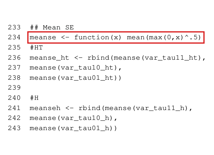
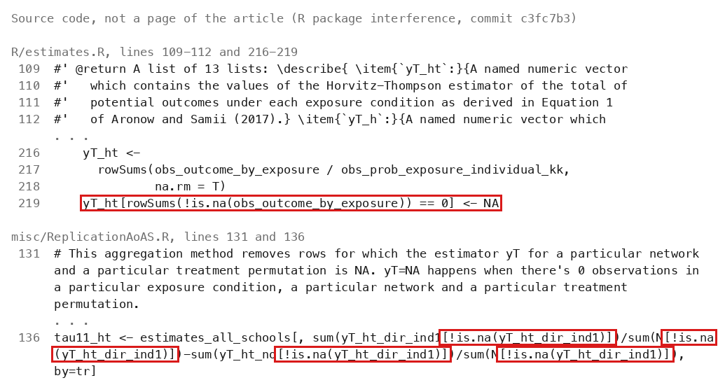
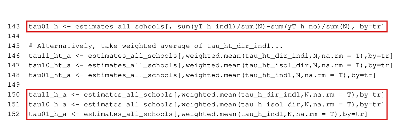
The sampler for Bernoulli designs in the later package rejects every assignment vector that repeats an earlier one, and the exposure probabilities are then computed with equal weights on the vectors kept, which distorts them (for N=100N=100, p=0.01p=0.01 and R=1000R=1000 the estimated probabilities of treatment average at least 0.018980.01898, against 0.010.01 under the design); the sampler should keep every independent draw.

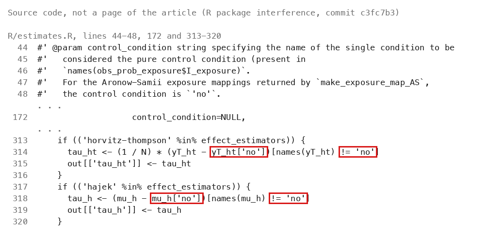
R package interference (commit c3fc7b3): R/make_tr_vec_bernoulli.R, function make_tr_vec_bernoulli_indiv, lines 169–187; R/make_exposure_prob.R, lines 83 and 88. The package DESCRIPTION credits Stephanie Zonszein, Cyrus Samii and P. M. Aronow; the corresponding formulas appear in Section 3, p. 1917 (PDF p. 6).

I disputed this classification, but as a rule, deferred to the models’ final judgment: see my comment and the history of this entry.

As printed

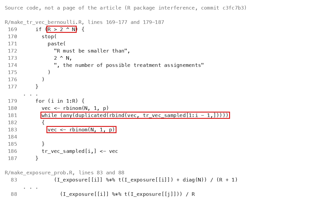
R/make_tr_vec_bernoulli.R, lines 169–177 (written on two lines):

if (R > 2 ^ N) { stop(paste("R must be smaller than", 2 ^ N,\texttt{if (}\colorbox{#ffe58a}{$\texttt{R > 2 \textasciicircum{} N}$}\texttt{) \{ stop(paste("R must be smaller than", 2 \textasciicircum{} N,}

", the number of possible treatment assignements")) }\texttt{", the number of possible treatment assignements")) \}}

Lines 179–187 (the inner loop joined on one line):

for (i in 1:R) {

vec <- rbinom(N, 1, p)

while (any(duplicated(rbind(vec, tr_vec_sampled[1:i - 1,])))) { vec <- rbinom(N, 1, p) }

tr_vec_sampled[i,] <- vec

}

R/make_exposure_prob.R, lines 83 and 88:

(I_exposure[[i]] %*% t(I_exposure[[i]]) + diag(N)) / (R + 1)

(I_exposure[[i]] %*% t(I_exposure[[j]])) / R

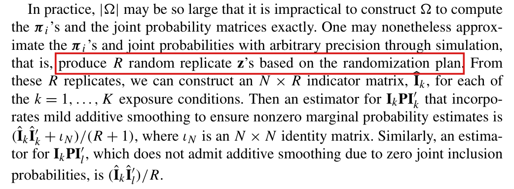
Section 3, p. 1917: “One may nonetheless approximate the πi\boldsymbol{\pi}_i's and joint probabilities with arbitrary precision through simulation, that is, produce RR random replicate z\mathbf{z}'s based on the randomization plan.”

The problem

I could not establish that this implementation was used for computations in the 2017 article. The loop on lines 181–185 redraws any assignment vector that repeats an earlier one. The RR vectors kept are then distinct, and they are not independent draws from the Bernoulli design. The function make_exposure_prob estimates the exposure probabilities by the unweighted frequencies over these vectors, as in the estimators (I^kI^k′+ιN)/(R+1)(\widehat{\mathbf{I}}_k\widehat{\mathbf{I}}_k'+\iota_N)/(R+1) and I^kI^l′/R\widehat{\mathbf{I}}_k\widehat{\mathbf{I}}_l'/R of Section 3. Unweighted frequencies estimate the probabilities under the design when the draws are independent, or when all assignment vectors are equally likely. Under a Bernoulli design with p≠1/2p\ne1/2 the assignment vectors are not equally likely, and the sampler keeps each of them at most once. A vector whose probability exceeds 1/R1/R is therefore under-represented in every sample, and less likely vectors take its place. This happens in populations of ordinary size. For N=100N=100 and p=0.01p=0.01 there are 21002^{100} assignment vectors, but the vector with no treated unit has probability (99/100)100≈0.366(99/100)^{100}\approx0.366. Two independent draws coincide with probability about 0.1350.135. In this design the less likely vectors have more treated units, and the estimated probabilities of treatment are too large for the numbers of replicates examined in the evidence. The estimated probabilities enter the Horvitz–Thompson estimates and their variance estimates as weights. The check on lines 169–177 follows from the same choice. The distinct vectors are exhausted at R=2NR=2^N, and the limit R→∞R\to\infty of Proposition 3.1 is not available to this sampler. The article names Bernoulli designs on a graph of bounded degree as a setting for its asymptotic results (p. 1926). Conditions 1–6 do not exclude the examples below, since a sequence of Bernoulli designs with pp fixed at 0.010.01 and bounded outcomes can satisfy them, with or without first-order interference on disjoint edges.

Evidence an exact counterexample

The evidence is an exact calculation for a design of ordinary size, a run of the unchanged code on that design, and an exact counterexample with two units.

Let N=100N=100 and p=1/100p=1/100, and let the exposure of a unit be its own treatment. Among RR distinct assignment vectors, at most one has no treated unit and at most 100100 have exactly one treated unit. Every further vector has at least two. For R=1000R=1000 the vectors kept then contain at least 100+2⋅899=1898100+2\cdot899=1898 treated entries. I call the fraction of the vectors kept in which a unit is treated its raw frequency of treatment. Averaged over the units, the raw frequency of treatment is at least 1898/(100⋅1000)=0.018981898/(100\cdot1000)=0.01898. This bound holds for every sample that the sampler can return, whatever the seed. The same count gives the other rows of the table.

Bernoulli design with N=100N=100 and p=0.01p=0.01: lower bounds that hold for every sample of RR distinct assignment vectors. The probability of treatment under the design is 0.010.01. Values that are not exact are rounded down.
RRTreated entriesAverage raw frequency of treatmentRelative excess over 0.010.01
1,0001{,}0001,8981{,}8980.0189800.01898089.80%89.80\%
1,5001{,}5002,8982{,}8980.0193200.01932093.20%93.20\%
10,00010{,}00024,84724{,}8470.0248470.024847148.47%148.47\%
10,59310{,}59326,62626{,}6260.0251350.025135151.35%151.35\%
100,000100{,}000294,847294{,}8470.0294840.029484194.84%194.84\%

Since the sampler treats the units symmetrically, the expected raw frequency of each unit obeys the same bounds. The diagonal entries that the package returns add one to each count and to RR, and for R=1000R=1000 their average is at least 1998/100100≈0.019961998/100100\approx0.01996. The raw joint frequency of treatment of a pair of units is the fraction of the vectors kept in which both units are treated. Counting the ordered pairs of treated units in the same way, I find that its average over the ordered pairs of units is at least 1798/(1000⋅100⋅99)≈0.00018161798/(1000\cdot100\cdot99)\approx0.0001816 for R=1000R=1000, against p2=0.0001p^2=0.0001. The value R=1500R=1500 is the number of replicates in the replication script of the package, and R=10,593R=10{,}593 is the number in the example after Proposition 4.1. The rows apply these numbers to the Bernoulli design. They do not recalculate any result of the article. For small RR the bound is not informative: for R=100R=100 it is 0.00990.0099. The distortion is present there as well. For R=2R=2 the expected raw frequency of treatment is 0.0110570.011057 to six decimals, which is 10.57%10.57\% above 0.010.01.

I ran the unchanged sampler with N=100N=100, p=0.01p=0.01, R=1000R=1000 and seed 101101. The 10001000 vectors kept are distinct and contain 22402240 treated entries. The average raw frequency of treatment is 0.02240.0224, and every unit is treated in at least 1212 of the vectors. On a graph of 5050 disjoint edges, the first-order exposure mapping of the package, which has the four exposures of Section 9, gives the following frequencies.

One run of the unchanged sampler (N=100N=100, p=0.01p=0.01, R=1000R=1000, seed 101) on 5050 disjoint edges: probabilities of the four exposures under the design and their raw frequencies in the run, averaged over the units.
ExposureProbability under the designAverage raw frequency
d11d_{11} (direct and indirect exposure)0.00010.00010.000320.00032
d10d_{10} (isolated direct exposure)0.00990.00990.022080.02208
d01d_{01} (indirect exposure)0.00990.00990.022080.02208
d00d_{00} (no exposure)0.98010.98010.955520.95552

Let every outcome under treatment equal 11, so that the total under treatment is 100100. Suppose that this total is estimated by the Horvitz–Thompson estimator with the probabilities that the package returns for this run. Given the vectors kept, the expectation of the estimator over the Bernoulli design is 44.3144.31, with an empty sum counted as zero. With independent draws, the identity of Appendix A.3 implies that the expectation over the replicates and the design is 100[1−(99/100)1001]100[1-(99/100)^{1001}].

For an exact counterexample with two units, let N=2N=2 and R=4R=4, and let each unit be treated with probability p=1/5p=1/5. The sampler then keeps each of the four assignment vectors once. Each unit is treated in half of them, although its probability of treatment under the design is 1/51/5. When the exposure of a unit is its own treatment, the package returns 3/53/5 and 1/51/5 for the marginal and joint probabilities of treatment. Their values under the design are 1/51/5 and 1/251/25. The distortion does not require that the sampler exhaust the assignment vectors: for R=2R=2 the expected raw frequency of treatment is 383/1260383/1260. At the observed assignment (1,0)(1,0) with both outcomes equal to 11, estimates() returns a Horvitz–Thompson total of 5/35/3 for the treated exposure with variance estimate 10/910/9, and the probabilities under the design give 55 and 2020. I confirmed these values by running the unchanged code.

The size of the distortion depends on the design. For p=1/2p=1/2 all assignment vectors are equally likely, and the raw frequencies are unbiased. If the first RR independent draws are distinct, the sampler returns exactly these draws. For N=1000N=1000, p=0.01p=0.01 and R=1500R=1500, the probability that two of them coincide is at most 0.00240.0024, and the expectations of the raw frequencies differ from those under independent draws by at most the same amount.

What survives

Section 3 and Proposition 3.1 are unaffected when the replicates are drawn independently from the randomization plan, and the two estimators of Section 3 are implemented as printed. The designs, the exposure mappings, the estimands and the results that take the exposure probabilities as known are unchanged. The simulation of Section 9 treats a fixed number of units chosen uniformly; the later package’s Table 1 replication script uses the permutation sampler, not this function, and does not establish which program generated the published table. That sampler also rejects repeats by default, but this distortion does not arise when equally likely vectors are sampled without replacement. No entry of Table 1 or Table 2 is shown to be affected by this error. I could not establish when the loop was introduced, who introduced it, or a causal connection between the code and Appendix A.1. I could not identify the code used to compute the exposure probabilities for the application of Section 10 or determine how its replicates were drawn. What is lost is the assurance that the probabilities computed from this sampler are those of the Bernoulli design. In sparse designs such as the one above they are not, and the Horvitz–Thompson estimates and variance estimates that use them inherit the error.

Corrected

R/make_tr_vec_bernoulli.R, lines 169–187, with the check of lines 169–177 and the inner loop of lines 181–185 deleted:

for (i in 1:R) {

vec <- rbinom(N, 1, p)

tr_vec_sampled[i,] <- vec

}

The sampler then keeps every independent draw, repeated vectors included, and RR is no longer limited by 2N2^N. The unit-level sampler’s documentation should say that repeated vectors are kept and remove its stated bound on RR. The two formulas of R/make_exposure_prob.R stay as they are. For any other design, each replicate should be an independent draw of the whole randomization, with all of its blocks and clusters, and the replicates should be drawn independently of the assignment observed in the experiment. If all distinct assignment vectors are enumerated instead, each must be weighted by its probability under the design, as in IkPIl′\mathbf{I}_k\mathbf{P}\mathbf{I}_l'. These weights alone do not correct a random subset of the vectors. Appendix A.1 itself says “without replacement”; that wording is addressed separately in the clarity note P013-E010 and does not establish use of this package for the publication.

Listing of source code with line numbers. In lines 169 to 177 of R/make_tr_vec_bernoulli.R, a red box marks the condition R > 2 ^ N of an if statement that stops the function with the message 'R must be smaller than 2 ^ N, the number of possible treatment assignements'. In lines 179 to 187, red boxes mark line 181, a while loop whose condition is that the new vector duplicates one of the vectors already sampled, and line 183, which draws a new vector with rbinom. Below, lines 83 and 88 of R/make_exposure_prob.R divide matrix products of exposure indicators by R + 1 and by R.
Source code of the package, not a page of the article: the check on the number of replicates (lines 169–177) and the sampling loop (lines 179–187) of make_tr_vec_bernoulli_indiv, and the two frequency formulas of R/make_exposure_prob.R (lines 83 and 88). The marked lines 181 and 183 redraw an assignment vector until it differs from every vector already kept, and the marked condition on line 169 limits RR to the number of distinct vectors.
Crop of the paragraph about approximating exposure probabilities by simulation. A red box marks the words 'produce R random replicate z's based on the randomization plan'. The paragraph ends with the estimators (I-hat-k I-hat-k-prime plus the identity matrix) divided by (R + 1), and I-hat-k I-hat-l-prime divided by R.
Section 3, p. 1917 (PDF p. 6): the original formulas used by the later package. The marked words describe replicates drawn from the randomization plan; the two estimators at the end of the paragraph weight the replicates equally. The formulas are correct for independent repetitions of the whole design; Appendix A.1’s conflicting without-replacement wording is addressed separately in the clarity note P013-E010.
My comment and the history of this entry

This was not a problem with this paper, but rather the later software package.

Suggested classification: not an error.

My position My comment above; I suggested that this is not an error.

The models’ position The scope of the audit includes a package that implements the paper’s method, and the defect in its assignment probabilities is verified. No published table is shown to be wrong: Moderate.

  1. Classification before my review (the classification when the audit was first completed, before I reviewed it): Moderate error.
  2. I commented and suggested that this is not an error.
  3. Independent evaluation. Incorporated in part. The entry now attributes the defect to the later package, gives the package’s full list of authors without assigning responsibility for the defect, and says that its use for the paper’s original calculations is not established. My suggestion that this is not an error was not adopted.

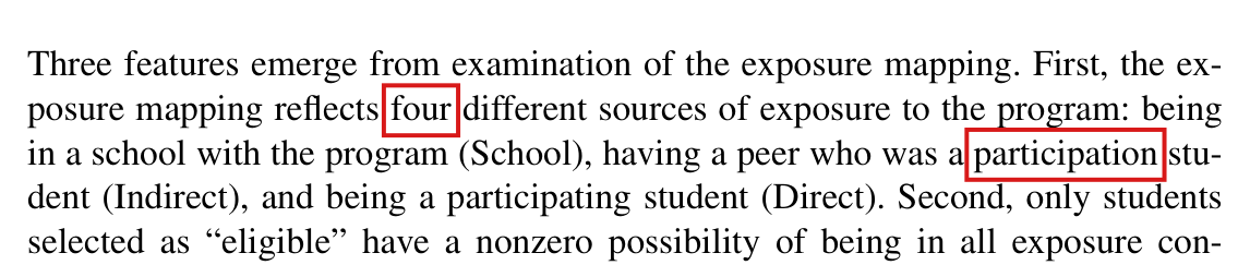
In a reconstruction on the public data, all twelve point estimates of Table 2 are reproduced with 342 of 2,050 students who have no recorded general wristband answer kept and scored zero; the article should state whether it uses this recorded orange-wristband outcome and disclose its missing-answer rule.

Section 10, first paragraph after Table 2, p. 1936 (PDF p. 25); Table 2, all rows

See also under Formal statements (Lean): P013-T23, P013-T24, P013-T27

My comment on this entry

As printed

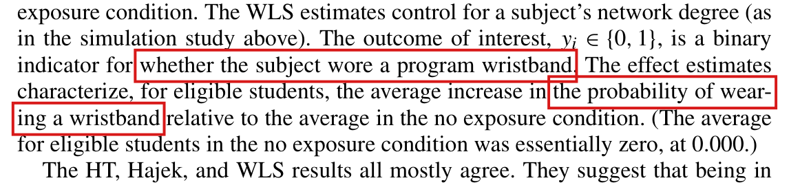
“The outcome of interest, yi∈{0,1}y_i\in\{0,1\}, is a binary indicator for whether the subject wore a program wristband. The effect estimates characterize, for eligible students, the average increase in the probability of wearing a wristband relative to the average in the no exposure condition.”

The problem

The article describes the outcome as whether the student wore a program wristband, measured by self-report (p. 1934), and it gives no rule for a student whose report is absent. On the public data release of the field experiment (ICPSR study 37070, version 2), the variable that reproduces Table 2 is an indicator for a recorded orange-wristband report. It is 00 or 11 for every student. The general wristband item of the second-wave survey, “I wore a Roots wristband this past week”, has no recorded answer for 342 of the 2,050 students of the reconstructed sample. Of these 342 students, 151 have no recorded second-wave survey, and 191 have a survey and no answer to the item. All 342 have the value 00 on the indicator. Among the three policies compared here, the twelve point estimates of Table 2 are reproduced to three decimals only when these students are kept in the sample with outcome 00. Without the 342 students the sample has 1,708 students, and without the 151 alone it has 1,899. In both cases none of the twelve estimates is reproduced. The article does not distinguish an observed negative answer from a zero recorded without an answer. For one student in six in this reconstruction, the zero stands where no answer to the general wristband item is recorded. Under the exposure assumptions for this recorded outcome, the reconstructed point estimates concern effects on a recorded report of wearing, with an absent report counted as zero. In the outcome model below, effects on wearing require a further condition that the article does not state: the students whose reports would be absent must contribute equally to the mean of wearing under the two exposures compared. The sizes that the text quotes, about 30 percentage points for direct exposure and 15 to 16 for indirect exposure, depend on the outcome definition. ICPSR notes that some released variables were changed. The authors' own outcome file is not public, and I could not check whether it codes these students as the public file does.

Evidence a recalculation from the source

The evidence is a recalculation on the public data, a derivation and an exact example. The recalculation uses the released code’s unblocked school-assignment generator, seed 123 and 10,000 draws, with the sampler that R used before version 3.6; the article describes school assignment as blocked. It keeps the eligible students whose five unsmoothed estimated exposure probabilities exceed 0.010.01, and it fits the WLS rows with one slope on network degree. This reconstruction has N=2,050N=2{,}050 students and, with the orange-wristband indicator as released, reproduces all twelve point estimates of Table 2 to three decimals. None of the eleven scripts released with the data computes Table 2, and the reconstruction is not the authors' calculation. Recall that the article limits the analysis to students with nonzero probabilities and does not state the cut-off of 0.010.01. Whether the published analysis used it is not determined.

Public data, reconstructed sample: the students with no recorded answer to the general wristband item, by observed exposure, with their share of NN and the number among them with no recorded second-wave survey. All 342 have the value 0 on the orange-wristband indicator.
Observed exposureNNNo answerShareNo survey
d000d_{000} (no exposure)1,03419819.1%78
d001d_{001} (school only)1572515.9%11
d011d_{011} (indirect)3485114.7%26
d101d_{101} (isolated direct)1992512.6%13
d111d_{111} (direct and indirect)3124313.8%23
All2,05034216.7%151
Point estimates of Table 2 as printed and as recalculated on the public data under three treatments of the students with no recorded general-item answer: kept and scored 0 (N=2,050N=2{,}050), without the 151 students with no recorded second-wave survey (N=1,899N=1{,}899), and without all 342 (N=1,708N=1{,}708).
EstimatorContrastPrintedKept as 0Without 151Without 342
HTτ(d001,d000)\tau(d_{001},d_{000})0.0570.0570.0620.069
τ(d011,d000)\tau(d_{011},d_{000})0.1540.1540.1660.185
τ(d101,d000)\tau(d_{101},d_{000})0.3050.3050.3290.366
τ(d111,d000)\tau(d_{111},d_{000})0.2990.2990.3230.359
Hajekτ(d001,d000)\tau(d_{001},d_{000})0.0580.0580.0620.069
τ(d011,d000)\tau(d_{011},d_{000})0.1540.1540.1670.181
τ(d101,d000)\tau(d_{101},d_{000})0.2920.2920.3100.332
τ(d111,d000)\tau(d_{111},d_{000})0.3070.3070.3300.355
WLSτ(d001,d000)\tau(d_{001},d_{000})0.0560.0560.0600.068
τ(d011,d000)\tau(d_{011},d_{000})0.1560.1560.1690.184
τ(d101,d000)\tau(d_{101},d_{000})0.2950.2950.3120.336
τ(d111,d000)\tau(d_{111},d_{000})0.3060.3060.3290.353

Every student removed in the last two columns has outcome 00. With the exposure probabilities held fixed, the numerators of the Horvitz–Thompson means are then unchanged, and only the divisor NN changes. Each HT contrast with these students kept equals 1708/2050=854/10251708/2050=854/1025 of its value without the 342 students, and 1899/20501899/2050 of its value without the 151. These ratios describe a change of divisor. They do not measure a bias.

To isolate the effect of absent reports, let Ri(d)R_i(d) indicate that usable wearing information for student ii is recorded under exposure dd, let yi(d)y_i(d) be the wearing outcome, and suppose the analyzed outcome is gi(d)=Ri(d) yi(d)g_i(d)=R_i(d)\,y_i(d). This model assumes that recorded reports equal wearing. Suppose also that yiy_i and RiR_i depend on the assignment only through the exposure and that the exposure probabilities used in the estimator are exact and positive. By Lemma 4.1 applied to gg, I have

E[μHT^(d)]=1N∑i=1Ngi(d)=μ(d)−L(d),L(d)=1N∑i=1N(1−Ri(d)) yi(d),\mathrm{E}\bigl[\widehat{\mu_{\mathrm{HT}}}(d)\bigr]=\frac{1}{N}\sum_{i=1}^{N}g_i(d)=\mu(d)-L(d),\qquad L(d)=\frac{1}{N}\sum_{i=1}^{N}\bigl(1-R_i(d)\bigr)\,y_i(d),

where the estimator is computed from the recorded outcomes and μ(d)\mu(d) is the mean of the wearing outcomes yi(d)y_i(d). Subtracting the same identity for d000d_{000}, I obtain

E[τHT^(dk,d000)]−τ(dk,d000)=L(d000)−L(dk).\mathrm{E}\bigl[\widehat{\tau_{\mathrm{HT}}}(d_k,d_{000})\bigr]-\tau(d_k,d_{000})=L(d_{000})-L(d_k).

This identity implies that the estimator with absent reports counted as zero is unbiased for the effect on wearing if and only if L(dk)=L(d000)L(d_k)=L(d_{000}). It suffices that under both exposures no student whose report would be absent would wear the wristband. Randomization, bounded outcomes and positive exposure probabilities do not imply this condition.

The exact example has two units with independent fair assignments and no interference. The first unit always reports, and its wearing outcome is 00 without treatment and 11 with it. The second unit never reports. Its wearing outcomes without and with treatment may be (0,0)(0,0), (0,1)(0,1) or (1,0)(1,0), and the recorded data are the same in the three cases under all four assignments. The effect on wearing is 1/21/2, 11 or 00. The estimator with the absent report counted as zero has expectation 1/21/2 in each case, and its bias is 00, −1/2-1/2 or 1/21/2. The estimator on the reporting unit alone has expectation 11. The recorded data therefore do not determine the sign of the bias.

Two limits apply. In the whole public file, 4,108 of the 24,471 records have no recorded answer to the general item, and four of them have the value 11 on the orange-wristband indicator. An absent answer to the general item does not prove that no information on colour was recorded. The released scripts do not show how the zeros arose: the cleaning script sets codes above 4 to missing and otherwise leaves the indicator as it is.

What survives

All twelve point estimates of Table 2 are reproduced on the public data under this coding, and so is the mean of zero in the no-exposure condition (0 of 1,034 students). The broad order of the effects is the same under each of the three treatments and for each estimator: school-only exposure, then indirect exposure, then the two direct exposures. This outcome-coding issue does not affect the estimators or the results of Sections 3 to 8, and the simulation of Section 9 has no absent outcomes. What changes is the definition of the outcome, and with it the estimand of Table 2 and the meaning of the sizes quoted on pp. 1936–1937. No bias in the effects on wearing is identified. This finding concerns point estimates only; a different treatment of these students would need its own standard errors.

Corrected

“The outcome of interest, yi∈{0,1}y_i\in\{0,1\}, is a binary indicator for whether the subject reported wearing an orange program wristband; a student with no recorded answer to the general wristband item, including a student with no recorded second-wave survey, is kept in the sample with yi=0y_i=0. Under the exposure-mapping assumptions for this recorded outcome, the effect estimates characterize, for eligible students, the average increase in the probability of such a recorded report relative to the average in the no exposure condition.”

In the public-data reconstruction with the strict 0.010.01 Monte Carlo screen described above, the students with no recorded general-item answer are 342 of 2,050, and 151 of them have no recorded second-wave survey. This wording is the correction if the authors' own outcome file codes these students as the public file does, which should be checked against that file. Under the outcome model above, retaining the wearing contrast requires L(dk)=L(d000)L(d_k)=L(d_{000}) for each contrast; otherwise it requires information or assumptions identifying the unrecorded outcomes and a new analysis with its standard errors.

Crop of seven lines of text after Table 2. The passage reads: The outcome of interest, y i in the set 0, 1, is a binary indicator for whether the subject wore a program wristband. The effect estimates characterize, for eligible students, the average increase in the probability of wearing a wristband relative to the average in the no exposure condition. (The average for eligible students in the no exposure condition was essentially zero, at 0.000.) Red boxes mark the words 'whether the subject wore a program wristband' and, across a line break, the words 'the probability of wearing a wristband'.
Section 10, first paragraph after Table 2, p. 1936 (PDF p. 25). The marked words define the outcome as whether the subject wore a program wristband, and the estimand as the probability of wearing a wristband. The passage gives no rule for a student whose report is absent.
Dot plot with twelve positions on the horizontal axis: the exposures d001, d011, d101 and d111, each compared with no exposure, for the HT, Hajek and WLS estimators. The vertical axis is the point estimate, with ticks from 0 to 0.4. At each position a black horizontal bar shows the value printed in Table 2, and a blue circle near the bar shows the estimate with students with no recorded general-item answer kept with their released outcome 0, N = 2,050. An orange square, higher, shows the estimate without the 151 students with no recorded second-wave survey, N = 1,899, and a green triangle, higher still, shows the estimate without the 342 students with no recorded general-item answer, N = 1,708. For example, for the HT estimate of d101 the printed value is 0.305, and the circle, square and triangle round to 0.305, 0.329 and 0.366. The title reads: Table 2 is reproduced on the public data only when students with no recorded answer are kept and scored as not wearing the wristband.
The twelve point estimates of Table 2, recalculated on the public data under three treatments of the students with no recorded answer to the general wristband item. The horizontal bars are the printed values. Among these three policies, only keeping these students with their released outcome zero (N=2,050N=2{,}050) reproduces all twelve estimates after rounding. Without the 151 students with no recorded second-wave survey (N=1,899N=1{,}899), or without all 342 students with no recorded general-item answer (N=1,708N=1{,}708), none does. The values are in the second table in the Evidence section above.
My comment and the history of this entry

Agreed.

  1. Classification before my review (the classification when the audit was first completed, before I reviewed it): Moderate error.
  2. I commented.
  3. Independent evaluation. No change was needed: my comment agrees with the entry.

Minor (17)

Real but inconsequential, for example a misprint that does not change a result.

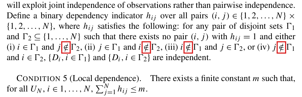
In the definition of the dependency indicator hijh_{ij}, the four signs ∉\notin should read ∈\in.

Section 6.2, definition of hijh_{ij} before Condition 5, p. 1925 (PDF p. 14)

See also under Formal statements (Lean): P013-T2, P013-T5, P013-T6

As printed

“Define a binary dependency indicator hijh_{ij} over all pairs (i,j)∈{1,2,…,N}×{1,2,…,N}(i,j)\in\{1,2,\ldots,N\}\times\{1,2,\ldots,N\}, where hijh_{ij} satisfies the following: for any pair of disjoint sets Γ1\Gamma_1 and Γ2⊆{1,…,N}\Gamma_2\subseteq\{1,\ldots,N\} such that there exists no pair (i,j)(i,j) with hij=1h_{ij}=1 and either (i) i∈Γ1i\in\Gamma_1 and j∉Γ2j\colorbox{#ffe58a}{$\notin$}\Gamma_2, (ii) j∈Γ1j\in\Gamma_1 and i∉Γ2i\colorbox{#ffe58a}{$\notin$}\Gamma_2, (iii) i∉Γ1i\colorbox{#ffe58a}{$\notin$}\Gamma_1 and j∈Γ2j\in\Gamma_2, or (iv) j∉Γ1j\colorbox{#ffe58a}{$\notin$}\Gamma_1 and i∈Γ2i\in\Gamma_2, {Di,i∈Γ1}\{D_i,i\in\Gamma_1\} and {Di,i∈Γ2}\{D_i,i\in\Gamma_2\} are independent.”

The problem

As printed, the two sets of exposures must be independent only when no edge of hh lies inside either set or leaves either set for the outside; edges between the two sets are allowed. This is not the condition that no edge joins the sets, and the requirement can be vacuous. If hh is the identity matrix, or the adjacency matrix of disjoint triangles, the premise holds only when both sets are empty. Every joint distribution of the exposures then satisfies the definition, with row sums 11 or 22. The printed definition therefore supports neither the statement on p. 1926 that Condition 5 subsumes Condition 4 nor the central limit theorem used for Proposition 6.2. The sentence before the definition, which announces “joint independence of observations rather than pairwise independence”, and the description on p. 1926 of a dependency graph of limited degree show what is meant.

Evidence an exact counterexample

The evidence is two exact counterexamples to the printed definition. First, let every unit receive the same fair Bernoulli exposure, Di=XD_i=X. With hh the identity matrix, the printed definition is satisfied and Condition 5 holds with m=1m=1. But every pair of units is dependent, which implies that ∑i=1N∑j=1Ngij=N2\sum_{i=1}^{N}\sum_{j=1}^{N}g_{ij}=N^2, and Condition 4 fails. Second, for N=36r2N=36r^2 let the number SS of treated units take the values 18r2−9r18r^2-9r, 18r218r^2 and 18r2+9r18r^2+9r with probabilities 1/181/18, 8/98/9 and 1/181/18, let the treated units be chosen uniformly given SS, and let Di=ZiD_i=Z_i, yi(1)=1y_i(1)=1 and yi(0)=0y_i(0)=0. Distinct units are pairwise independent, and Conditions 1–4 hold. Condition 5 holds as printed, with hh the adjacency matrix of disjoint triangles and m=2m=2. Condition 6 holds, since NVar⁡[τ^HT]=1N\operatorname{Var}[\widehat{\tau}_{\mathrm{HT}}]=1 for every rr. The estimator standardized by its true standard deviation takes the values −3-3, 00 and 33 with probabilities 1/181/18, 8/98/9 and 1/181/18 for every rr, which is not a normal limit. The interval of Proposition 6.2 with critical value 22 has coverage exactly 8/98/9 for every r≥5r\ge5, which is below its nominal level. Neither example satisfies the corrected definition.

Applying the corrected definition to two singletons, I find that any two dependent units are adjacent. Since the row sums are at most mm, I obtain ∑i∑jgij≤N(m+1)=O(N)\sum_{i}\sum_{j}g_{ij}\le N(m+1)=O(N), which is the statement on p. 1926 that Condition 5 subsumes Condition 4.

What survives

The unbiasedness results, the exact variance formulas, Proposition 5.6 and Proposition 6.1, which uses Conditions 3 and 4, do not involve hijh_{ij}. With the four signs corrected the definition is the dependency-graph condition that p. 1926 describes and that Appendix A.7 uses, and no reported number depends on it. The correction does not by itself settle Proposition 6.2, which is the subject of P013-E001.

Corrected

Define a binary dependency indicator hijh_{ij} over all pairs (i,j)∈{1,2,…,N}×{1,2,…,N}(i,j)\in\{1,2,\ldots,N\}\times\{1,2,\ldots,N\}, where hijh_{ij} satisfies the following: for any pair of disjoint sets Γ1\Gamma_1 and Γ2⊆{1,…,N}\Gamma_2\subseteq\{1,\ldots,N\} such that there exists no pair (i,j)(i,j) with hij=1h_{ij}=1 and either (i) i∈Γ1i\in\Gamma_1 and j∈Γ2j\colorbox{#ffe58a}{$\in$}\Gamma_2, (ii) j∈Γ1j\in\Gamma_1 and i∈Γ2i\colorbox{#ffe58a}{$\in$}\Gamma_2, (iii) i∈Γ1i\colorbox{#ffe58a}{$\in$}\Gamma_1 and j∈Γ2j\in\Gamma_2, or (iv) j∈Γ1j\colorbox{#ffe58a}{$\in$}\Gamma_1 and i∈Γ2i\in\Gamma_2, {Di,i∈Γ1}\{D_i,i\in\Gamma_1\} and {Di,i∈Γ2}\{D_i,i\in\Gamma_2\} are independent.

For symmetric hh the definition reads as follows. For every pair of disjoint sets Γ1\Gamma_1 and Γ2⊆{1,…,N}\Gamma_2\subseteq\{1,\ldots,N\}, if hij=0h_{ij}=0 for all i∈Γ1i\in\Gamma_1 and j∈Γ2j\in\Gamma_2, then the random vectors (Di)i∈Γ1(D_i)_{i\in\Gamma_1} and (Dj)j∈Γ2(D_j)_{j\in\Gamma_2} are independent. Condition 5 is unchanged: there exists a finite constant mm such that, for all UNU_N and all i∈{1,…,N}i\in\{1,\ldots,N\}, ∑j=1Nhij≤m\sum_{j=1}^{N}h_{ij}\le m. Independence of each pair of nonadjacent units would not suffice; the vectors of exposures of the two sets must be independent.

Crop of the paragraph that defines the binary dependency indicator h_ij, followed by Condition 5 (Local dependence). Red boxes mark the four 'not an element of' signs in clauses (i) j not in Gamma_2, (ii) i not in Gamma_2, (iii) i not in Gamma_1 and (iv) j not in Gamma_1.
Section 6.2, definition of hijh_{ij} and Condition 5, p. 1925 (PDF p. 14). The four marked signs are printed as ∉\notin and should be ∈\in.

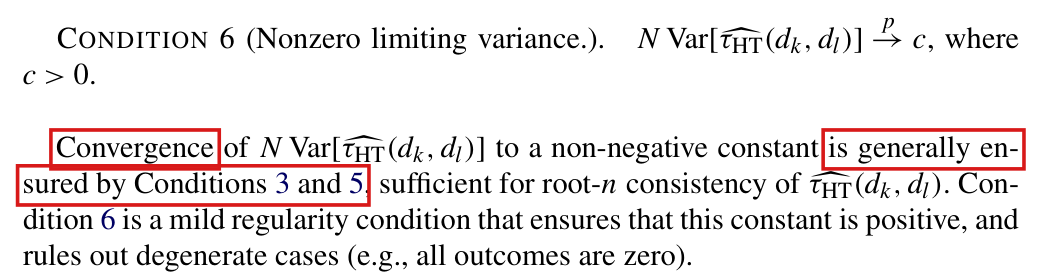
Even when the conservative variance estimator concentrates around its expectation, it need not converge, and the variance ratio and the studentized statistic tt need not have limits; coverage of at least 1−α1 - \alpha in the limit inferior follows from a one-sided bound once concentration and the true-variance central limit theorem hold.

Appendix A.7, proof of Proposition 6.2, first and last paragraphs, p. 1943 (PDF p. 32)

See also under Formal statements (Lean): P013-T7, P013-T8

As printed

First paragraph of A.7. By Proposition 5.6, E[NVar⁡^[τ^HT(dk,dl)]]≥NVar⁡[τ^HT(dk,dl)]\mathrm{E}[N\widehat{\operatorname{Var}}[\widehat{\tau}_{\mathrm{HT}}(d_k,d_l)]]\ge N\operatorname{Var}[\widehat{\tau}_{\mathrm{HT}}(d_k,d_l)]. Thus, by Chebyshev’s inequality, Var⁡[NVar⁡^[τ^HT(dk,dl)]]→p0\operatorname{Var}[N\widehat{\operatorname{Var}}[\widehat{\tau}_{\mathrm{HT}}(d_k,d_l)]]\xrightarrow{p}0 is sufficient to establish convergence of NVar⁡^[τ^HT(dk,dl)]N\widehat{\operatorname{Var}}[\widehat{\tau}_{\mathrm{HT}}(d_k,d_l)] to a value greater than or equal to NVar⁡[τ^HT(dk,dl)]N\operatorname{Var}[\widehat{\tau}_{\mathrm{HT}}(d_k,d_l)], which is itself nonzero by Condition 6.

Last paragraph of A.7. Define

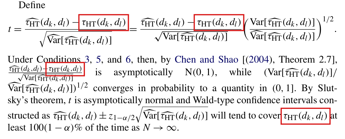
t=τ^HT(dk,dl)−τHT(dk,dl)Var⁡^[τ^HT(dk,dl)]=τ^HT(dk,dl)−τHT(dk,dl)Var⁡[τ^HT(dk,dl)](Var⁡[τ^HT(dk,dl)]Var⁡^[τ^HT(dk,dl)])1/2.t=\frac{\widehat{\tau}_{\mathrm{HT}}(d_k,d_l)-\tau_{\mathrm{HT}}(d_k,d_l)}{\sqrt{\widehat{\operatorname{Var}}[\widehat{\tau}_{\mathrm{HT}}(d_k,d_l)]}}=\frac{\widehat{\tau}_{\mathrm{HT}}(d_k,d_l)-\tau_{\mathrm{HT}}(d_k,d_l)}{\sqrt{\operatorname{Var}[\widehat{\tau}_{\mathrm{HT}}(d_k,d_l)]}}\left(\frac{\operatorname{Var}[\widehat{\tau}_{\mathrm{HT}}(d_k,d_l)]}{\widehat{\operatorname{Var}}[\widehat{\tau}_{\mathrm{HT}}(d_k,d_l)]}\right)^{1/2}.

Under Conditions 3, 5, and 6, then, by Chen and Shao [(2004), Theorem 2.7], τ^HT(dk,dl)−τHT(dk,dl)Var⁡[τ^HT(dk,dl)]\frac{\widehat{\tau}_{\mathrm{HT}}(d_k,d_l)-\tau_{\mathrm{HT}}(d_k,d_l)}{\sqrt{\operatorname{Var}[\widehat{\tau}_{\mathrm{HT}}(d_k,d_l)]}} is asymptotically N(0,1)\mathrm{N}(0,1), while (Var⁡[τ^HT(dk,dl)]/Var⁡^[τ^HT(dk,dl)])1/2(\operatorname{Var}[\widehat{\tau}_{\mathrm{HT}}(d_k,d_l)]/\widehat{\operatorname{Var}}[\widehat{\tau}_{\mathrm{HT}}(d_k,d_l)])^{1/2} converges in probability to a quantity in (0,1](0,1]. By Slutsky’s theorem, tt is asymptotically normal and Wald-type confidence intervals constructed as τ^HT(dk,dl)±z1−α/2Var⁡^[τ^HT(dk,dl)]\widehat{\tau}_{\mathrm{HT}}(d_k,d_l)\pm z_{1-\alpha/2}\sqrt{\widehat{\operatorname{Var}}[\widehat{\tau}_{\mathrm{HT}}(d_k,d_l)]} will tend to cover τHT(dk,dl)\tau_{\mathrm{HT}}(d_k,d_l) at least 100(1−α)%100(1-\alpha)\% of the time as N→∞N\to\infty.

The problem

Let VNV_N denote the variance of the HT estimator of the effect, and let V^N\widehat V_N denote the variance estimator (11). The last paragraph of A.7 uses three premises: the estimator standardized by VN\sqrt{V_N} is asymptotically standard normal; NVNN V_N tends to c>0c > 0 (Condition 6); and NV^NN \widehat V_N has expectation at least NVNN V_N (Proposition 5.6) and variance tending to zero. By Chebyshev’s inequality, the third premise implies that NV^NN \widehat V_N is close to its own expectation with probability tending to one. It does not imply convergence “to a value”. The expectation of NV^NN \widehat V_N exceeds NVNN V_N by the bias of the conservative estimator. No condition controls how this bias varies with NN, and the expectation may fail to converge. The opening inference of A.7 is then not valid. The two claims of the last paragraph that rest on it can fail under Conditions 3, 5 and 6: that the ratio (VN/V^N)1/2(V_N/\widehat V_N)^{1/2} converges in probability to a quantity in (0,1](0,1], and that tt is asymptotically normal by Slutsky’s theorem.

The conclusion of the paragraph does not need these limits. Coverage of at least 100(1−α)%100(1-\alpha)\% for large NN is a lower bound, and a one-sided bound on NV^NN \widehat V_N is enough to obtain it. This finding takes the three premises as given. Whether the variance of NV^NN \widehat V_N tends to zero under Conditions 3, 5 and 6 is a separate question, treated in P013-E001.

Evidence an exact counterexample

The evidence is an exact counterexample to the two printed claims and a derivation of the corrected bound.

Counterexample. Set n0=0n_0 = 0 and nr=22rn_r = 2^{2^r} for r≥1r \ge 1. The units are the positive integers, the population of size NN is {1,…,N}\{1, \ldots, N\}, and block rr consists of the units nr−1+1,…,nrn_{r-1}+1, \ldots, n_r. There are two exposures, dk=1d_k = 1 and dl=0d_l = 0. In a block with rr odd, every unit has potential outcomes (yi(1),yi(0))=(1,1)(y_i(1), y_i(0)) = (1,1). In a block with rr even, the units alternate between (2,0)(2,0) and (0,2)(0,2), beginning with (2,0)(2,0). The assignments ZiZ_i are independent with Pr⁡(Zi=1)=1/2\Pr(Z_i = 1) = 1/2, and Di=ZiD_i = Z_i. Conditions 1 and 2 hold. Since the outcomes are at most 22 and every exposure probability is 1/21/2, Condition 3 holds. With hij=1{i=j}h_{ij} = \mathbf{1}\{i = j\} and m=1m = 1, Condition 5 holds, and every joint exposure probability of two distinct units equals 1/41/4.

Let τ^N\widehat\tau_N and τN\tau_N be the estimator and the estimand in the population of size NN, and set Ri=2Zi−1R_i = 2 Z_i - 1. Since yi(1)+yi(0)=2y_i(1) + y_i(0) = 2 for every unit, I have

τ^N−τN=2N∑i=1NRi,NVN=4\widehat\tau_N - \tau_N = \frac{2}{N} \sum_{i=1}^{N} R_i , \qquad N V_N = 4

for every NN, so Condition 6 holds with c=4c = 4, and the standardized estimator is asymptotically standard normal. Substituting the exposure probabilities into (7), (10) and (11), I obtain V^N=4N−2∑i≤NYi2\widehat V_N = 4 N^{-2} \sum_{i \le N} Y_i^2. Let bNb_N be the number of units i≤Ni \le N in blocks with rr even, and set fN=bN/Nf_N = b_N/N. A unit in an odd block has Yi2=1Y_i^2 = 1, and a unit in an even block has Yi2=2+2siRiY_i^2 = 2 + 2 s_i R_i with si=1s_i = 1 or si=−1s_i = -1. Taking the expectation and the variance of the sum, I find

E[NV^N]=4+4fN,Var⁡(NV^N)=64 bNN2≤64N.\mathbb{E}[N \widehat V_N] = 4 + 4 f_N , \qquad \operatorname{Var}(N \widehat V_N) = \frac{64 \, b_N}{N^2} \le \frac{64}{N} .

The variance tends to zero, as the printed argument requires. The expectation does not converge: at the end of block rr, I have fnr≤nr−1/nrf_{n_r} \le n_{r-1}/n_r for rr odd and 1−fnr≤nr−1/nr1 - f_{n_r} \le n_{r-1}/n_r for rr even, and nr−1/nr=2−2r−1n_{r-1}/n_r = 2^{-2^{r-1}} for r≥2r \ge 2, which tends to zero.

The example at the ends of the first four blocks. The scaled variance NVNN V_N equals 44 in every row.
rrN=nrN = n_rbNb_NE[NV^N]\mathbb{E}[N \widehat V_N]Var⁡(NV^N)\operatorname{Var}(N \widehat V_N)
1144004400
22161612127733
33256256121267/16≈4.1967/16 \approx 4.193/2563/256
446553665536652926529232707/4096≈7.9932707/4096 \approx 7.9916323/1677721616323/16777216

Along N=nrN = n_r with rr odd, NV^NN \widehat V_N tends to 44 in probability, the ratio (VN/V^N)1/2(V_N/\widehat V_N)^{1/2} tends to 11, and tt converges in distribution to N(0,1)\mathcal{N}(0,1). Along N=nrN = n_r with rr even, NV^NN \widehat V_N tends to 88 in probability, the ratio tends to 1/21/\sqrt{2}, and tt converges in distribution to N(0,1/2)\mathcal{N}(0,1/2). Neither the ratio nor tt has a limit along the full sequence. Enumerating all 2N2^N assignments for each N≤10N \le 10 in exact arithmetic, I obtain the same values from the printed expressions (7), (10) and (11).

Corrected bound. Set vN=NVNv_N = N V_N, WN=NV^NW_N = N \widehat V_N and ZN=(τ^N−τN)/VNZ_N = (\widehat\tau_N - \tau_N)/\sqrt{V_N}. Suppose that vN→c>0v_N \to c > 0, that ZNZ_N converges in distribution to N(0,1)\mathcal{N}(0,1), that E[WN]≥vN\mathbb{E}[W_N] \ge v_N, and that Var⁡(WN)→0\operatorname{Var}(W_N) \to 0. I count a negative variance estimate as noncoverage in the probabilities below. Fix ϵ∈(0,1)\epsilon \in (0,1). If WN<(1−ϵ)vNW_N < (1-\epsilon) v_N, then E[WN]−WN>ϵvN\mathbb{E}[W_N] - W_N > \epsilon v_N. By Chebyshev’s inequality, this implies that

Pr⁡(WN<(1−ϵ)vN)≤Var⁡(WN)ϵ2vN2⟶0.\Pr\bigl( W_N < (1-\epsilon) v_N \bigr) \le \frac{\operatorname{Var}(W_N)}{\epsilon^2 v_N^2} \longrightarrow 0 .

On the complementary event, V^N\widehat V_N is positive and V^N/VN≥1−ϵ\sqrt{\widehat V_N / V_N} \ge \sqrt{1-\epsilon}. With z=z1−α/2z = z_{1-\alpha/2}, I have

Pr⁡(∣τ^N−τN∣≤zV^N)≥Pr⁡(∣ZN∣≤z1−ϵ)−Pr⁡(WN<(1−ϵ)vN).\Pr\bigl( |\widehat\tau_N - \tau_N| \le z \sqrt{\widehat V_N} \bigr) \ge \Pr\bigl( |Z_N| \le z \sqrt{1-\epsilon} \bigr) - \Pr\bigl( W_N < (1-\epsilon) v_N \bigr) .

Taking the limit inferior and using the convergence of ZNZ_N, I obtain

lim inf⁡N→∞Pr⁡(∣τ^N−τN∣≤zV^N)≥2Φ(z1−ϵ)−1.\liminf_{N \to \infty} \Pr\bigl( |\widehat\tau_N - \tau_N| \le z \sqrt{\widehat V_N} \bigr) \ge 2 \Phi\bigl( z \sqrt{1-\epsilon} \bigr) - 1 .

Since ϵ\epsilon is arbitrary, the limit inferior of the coverage is at least 2Φ(z)−1=1−α2\Phi(z) - 1 = 1 - \alpha. Note that the argument uses no limit for WNW_N and no independence between ZNZ_N and WNW_N.

What survives

The HT estimator, the variance estimator (11), unbiasedness, Proposition 5.6, Proposition 6.1 and the central limit theorem for the estimator standardized by its true variance are unaffected. The coverage conclusion of Proposition 6.2 holds as a lower bound on the limit inferior of the coverage, under the three premises of the last paragraph of A.7 and with no new assumption. The proof no longer gives a single limiting law for tt or a single limit for the coverage. In the example, the coverage tends to 1−α1 - \alpha along one subsequence and to 2Φ(z1−α/22)−12\Phi(z_{1-\alpha/2}\sqrt{2}) - 1 along the other. To keep the printed limit, one would add the assumption that E[NV^N]\mathbb{E}[N \widehat V_N] converges to a finite s≥cs \ge c; then the ratio tends to c/s\sqrt{c/s} and tt converges in distribution to N(0,c/s)\mathcal{N}(0, c/s). No number in Table 1 or Table 2 changes.

Corrected

First paragraph of A.7. By Proposition 5.6, E[NVar⁡^[τ^HT(dk,dl)]]≥NVar⁡[τ^HT(dk,dl)]\mathrm{E}[N\widehat{\operatorname{Var}}[\widehat{\tau}_{\mathrm{HT}}(d_k,d_l)]]\ge N\operatorname{Var}[\widehat{\tau}_{\mathrm{HT}}(d_k,d_l)]. Thus, by Chebyshev’s inequality, Var⁡[NVar⁡^[τ^HT(dk,dl)]]→p0\operatorname{Var}[N\widehat{\operatorname{Var}}[\widehat{\tau}_{\mathrm{HT}}(d_k,d_l)]]\xrightarrow{p}0 is sufficient to establish concentration of NVar⁡^[τ^HT(dk,dl)]N\widehat{\operatorname{Var}}[\widehat{\tau}_{\mathrm{HT}}(d_k,d_l)] around its expectation, which is greater than or equal to NVar⁡[τ^HT(dk,dl)]N\operatorname{Var}[\widehat{\tau}_{\mathrm{HT}}(d_k,d_l)], which is itself nonzero by Condition 6. The expectation need not converge, and no limit of the variance estimator is used below.

Last paragraph of A.7. Let τ^N=τ^HT(dk,dl)\widehat\tau_N = \widehat{\tau}_{\mathrm{HT}}(d_k,d_l) and τN=τHT(dk,dl)\tau_N = \tau_{\mathrm{HT}}(d_k,d_l), and set VN=Var⁡[τ^N]V_N = \operatorname{Var}[\widehat\tau_N], V^N=Var⁡^[τ^N]\widehat V_N = \widehat{\operatorname{Var}}[\widehat\tau_N], vN=NVNv_N = N V_N, WN=NV^NW_N = N \widehat V_N and ZN=(τ^N−τN)/VNZ_N = (\widehat\tau_N - \tau_N)/\sqrt{V_N}. Under Conditions 3, 5, and 6, then, by Chen and Shao [(2004), Theorem 2.7], ZNZ_N is asymptotically N(0,1)\mathrm{N}(0,1). By Condition 6, vN→c>0v_N \to c > 0; by Proposition 5.6, E[WN]≥vN\mathrm{E}[W_N] \ge v_N; for this step, assume the concentration premise Var⁡(WN)→0\operatorname{Var}(W_N) \to 0. For each ϵ∈(0,1)\epsilon \in (0,1), Chebyshev’s inequality gives

Pr⁡(WN<(1−ϵ)vN)≤Var⁡(WN)ϵ2vN2⟶0,\colorbox{#ffe58a}{$\displaystyle \Pr\bigl( W_N < (1-\epsilon) v_N \bigr) \le \frac{\operatorname{Var}(W_N)}{\epsilon^2 v_N^2} \longrightarrow 0 ,$}

I count a negative variance estimate as noncoverage; the bound shows that its probability tends to zero. On the complementary event V^N/VN≥1−ϵ\sqrt{\widehat V_N/V_N} \ge \sqrt{1-\epsilon}. With z=z1−α/2z = z_{1-\alpha/2}, it follows that

lim inf⁡N→∞Pr⁡(∣τ^N−τN∣≤zV^N)≥2Φ(z1−ϵ)−1.\colorbox{#ffe58a}{$\displaystyle \liminf_{N \to \infty} \Pr\bigl( |\widehat\tau_N - \tau_N| \le z \sqrt{\widehat V_N} \bigr) \ge 2 \Phi\bigl( z \sqrt{1-\epsilon} \bigr) - 1 .$}

Letting ϵ↓0\epsilon \downarrow 0, Wald-type confidence intervals constructed as τ^HT(dk,dl)±z1−α/2Var⁡^[τ^HT(dk,dl)]\widehat{\tau}_{\mathrm{HT}}(d_k,d_l)\pm z_{1-\alpha/2}\sqrt{\widehat{\operatorname{Var}}[\widehat{\tau}_{\mathrm{HT}}(d_k,d_l)]} cover τHT(dk,dl)\tau_{\mathrm{HT}}(d_k,d_l) with probability at least 1−α1-\alpha in the limit inferior as N→∞N\to\infty. No limit is asserted for the variance ratio or for the statistic tt.

Crop of the six lines that end the proof of Proposition 6.2. The text says that under Conditions 3, 5, and 6, by Chen and Shao (2004), Theorem 2.7, the estimator minus its target, divided by the square root of its variance, is asymptotically N(0, 1), while the square root of the ratio of the variance to the estimated variance converges in probability to a quantity in (0, 1]. It continues: By Slutsky's theorem, t is asymptotically normal and Wald-type confidence intervals constructed as the estimator plus or minus z times the square root of the estimated variance will tend to cover the target at least 100(1 - alpha) percent of the time as N tends to infinity. Red outlines surround the words converges in probability to a quantity in (0, 1] and the words t is asymptotically normal.
Appendix A.7, last paragraph, p. 1943 (PDF p. 32). The outlines mark the claim that the variance ratio converges in probability to a quantity in (0,1](0,1] and the claim that tt is asymptotically normal.

The difference estimator of expressions (12) and (13) is location equivariant if a constant added to every outcome is also added to every prediction; Section 7.1 states the property without this condition, and it fails in general if the predictions are held numerically fixed, because the estimated total then changes by the constant times the realized sum of the weights I(Di=dk)/πi(dk)\mathbf{I}(D_i=d_k)/\pi_i(d_k), which need not equal the constant times NN.

Section 7.1, p. 1927 (PDF p. 16): first paragraph, and the sentence after expression (13)

See also under Formal statements (Lean): P013-T21, P013-T22

As printed

“In addition, the difference estimator addresses the problem of location noninvariance that afflicts Horvitz–Thompson-type estimators [Fuller (2009), pages 9–10].”

“We have some predefined function g(xi,ξi(dk))→Rg(\mathbf{x}_i,\boldsymbol{\xi}_i(d_k))\to\mathbb{R}, where ξi\boldsymbol{\xi}_i is a parameter vector. Ideally g(⋅)g(\cdot) is calibrated on auxiliary data to produce values that approximate yi(dk)y_i(d_k). … Define

(12)yGT^(dk)=∑i=1NI(Di=dk)Yiπi(dk)−∑i=1NI(Di=dk)g(xi,ξi(dk))πi(dk)+∑i=1Ng(xi,ξi(dk)),(12)\qquad \widehat{y^T_G}(d_k)=\sum_{i=1}^N\mathbf{I}(D_i=d_k)\frac{Y_i}{\pi_i(d_k)}-\sum_{i=1}^N\mathbf{I}(D_i=d_k)\frac{g(\mathbf{x}_i,\boldsymbol{\xi}_i(d_k))}{\pi_i(d_k)}+\sum_{i=1}^N g(\mathbf{x}_i,\boldsymbol{\xi}_i(d_k)),

…”

“Middleton and Aronow (2011) and Aronow and Middleton (2013) demonstrate that yGT^(dk)\widehat{y^T_G}(d_k) is location invariant. Variance estimation proceeds as in Section 5 using εi(dk)\varepsilon_i(d_k) in place of yi(dk)y_i(d_k) as long as g(xi,ξi(dk))g(\mathbf{x}_i,\boldsymbol{\xi}_i(d_k)) is fixed.”

The problem

Section 7.1 says twice that the difference estimator does not depend on the origin of the outcome scale in the way that Horvitz–Thompson estimators do. The first statement is in its first paragraph. The second follows expression (13) and attributes the property to two cited works. Neither states a condition. For an estimated total the property is equivariance. If a constant cc is added to every potential outcome, the estimated total should increase by cNcN, and the estimated contrast between two exposures should not change. Whether expression (12) has this property depends on what happens to the predictions g(xi,ξi(dk))g(\mathbf{x}_i,\boldsymbol{\xi}_i(d_k)) when the outcomes are shifted, and the section does not say. It calls the predictions “predefined” and “fixed”, and these words refer to the randomization, not to the origin of the outcome scale. If the predictions are shifted by cc with the outcomes, the property holds. If they are held numerically fixed, which the printed assumptions allow, it fails in general. The estimated total then increases by cWkcW_k, where Wk=∑i=1NI(Di=dk)/πi(dk)W_k=\sum_{i=1}^N\mathbf{I}(D_i=d_k)/\pi_i(d_k) is the realized sum of the weights. The error c (Wk−N)c\,(W_k-N) varies with the assignment. Aronow and Middleton (2013) show the property for predictions that are recoded by the same transformation as the outcomes. The sentence after expression (13) reports this conditional result without its condition.

Evidence an exact counterexample

The evidence is a derivation of the exact change of the estimator under a shift of the outcomes, an exact counterexample with the predictions held numerically fixed, and a check of the cited works.

Let gi=g(xi,ξi(dk))g_i=g(\mathbf{x}_i,\boldsymbol{\xi}_i(d_k)), wi=I(Di=dk)/πi(dk)w_i=\mathbf{I}(D_i=d_k)/\pi_i(d_k) and Wk=∑i=1NwiW_k=\sum_{i=1}^N w_i. By Condition 2, I have

yGT^(dk)=∑i=1Nwi (yi(dk)−gi)+∑i=1Ngi.\widehat{y^T_G}(d_k)=\sum_{i=1}^N w_i\,\bigl(y_i(d_k)-g_i\bigr)+\sum_{i=1}^N g_i .

Suppose that every potential outcome increases by cc and that each prediction gig_i changes by hih_i, while the design, the exposures and the covariates stay the same. Substituting into the display, I obtain that the estimated total changes by

∑i=1Nwi (c−hi)+∑i=1Nhi=cWk+∑i=1N(1−wi)hi.\sum_{i=1}^N w_i\,(c-h_i)+\sum_{i=1}^N h_i=cW_k+\sum_{i=1}^N(1-w_i)h_i .

Since ∑i=1N(1−wi)=N−Wk\sum_{i=1}^N(1-w_i)=N-W_k, this change differs from cNcN by

∑i=1N(1−wi)(hi−c).\sum_{i=1}^N(1-w_i)(h_i-c).

If hi=ch_i=c for every ii, each term vanishes. The residuals yi(dk)−giy_i(d_k)-g_i are unchanged, the estimated total increases by cNcN on every assignment, and the estimated contrast [yGT^(dk)−yGT^(dl)]/N[\widehat{y^T_G}(d_k)-\widehat{y^T_G}(d_l)]/N between two exposures does not change. If hi=0h_i=0 for every ii, the estimated total increases by cWkcW_k, the error is c (Wk−N)c\,(W_k-N), and the estimated contrast changes by c (Wk−Wl)/Nc\,(W_k-W_l)/N. Since E[wi]=1\mathrm{E}[w_i]=1, the error has expectation zero, but for c≠0c\ne0 it vanishes on a given assignment only if Wk=NW_k=N.

For the counterexample, let N=3N=3 with no interference. One unit is selected, with probabilities 1/41/4, 1/41/4 and 1/21/2 for the three units. For the selected unit Di=dkD_i=d_k, and for the other two Di=dlD_i=d_l. Then πi(dk)\pi_i(d_k) equals 1/41/4, 1/41/4, 1/21/2 and πi(dl)\pi_i(d_l) equals 3/43/4, 3/43/4, 1/21/2, and Conditions 1 and 2 hold. Let the potential outcomes be (2,3,5)(2,3,5) under both exposures, and let the predictions be the fixed numbers (2,3,5)(2,3,5) for both exposures. The predictions do not vary with the assignment, their covariance with ZiZ_i is zero, and they equal the outcomes. Both estimated totals equal 1010 on every assignment, and the estimated contrast is 00. I now add c=1c=1 to every potential outcome and keep the predictions. Both true totals become 1313, and the true contrast τ(dk,dl)\tau(d_k,d_l) remains 00. Every residual equals 11, and the estimated totals are 10+Wk10+W_k and 10+Wl10+W_l.

The three-unit example after 11 is added to every outcome, with the predictions held numerically fixed at (2,3,5)(2,3,5): the realized sums of the weights, the two estimated totals and the estimated contrast. Both true totals equal 1313 and the true contrast equals 00.
Selected unitProbabilityWkW_kWlW_lyGT^(dk)\widehat{y^T_G}(d_k)yGT^(dl)\widehat{y^T_G}(d_l)Estimated contrast
11/41/44410/310/3141440/340/32/92/9
21/41/44410/310/3141440/340/32/92/9
31/21/2228/38/3121238/338/3−2/9-2/9

Neither estimated total increases by cN=3cN=3 on any assignment, and the estimated contrast is never 00. Both estimated totals have expectation 1313 and remain unbiased. The variance of the estimated contrast rises from 00 to 4/814/81. If 11 is also added to every prediction, both estimated totals equal 1313 and the estimated contrast equals 00 on every assignment. Conditions 1–6 do not restore the property. Independent copies of this design, with every outcome and every prediction equal to 11, form a sequence that satisfies them with NVar⁡[τ^HT(dk,dl)]=4/27N\operatorname{Var}[\widehat{\tau}_{\mathrm{HT}}(d_k,d_l)]=4/27, and a shift of the outcomes alone still changes the estimated contrast.

Where I could consult the cited works, they state the property with the condition. Aronow and Middleton (2013) recode the outcomes as Yi∗=b0+b1YiY_i^*=b_0+b_1Y_i (p. 139) and, in their Appendix C (p. 151), require that the “predictive function will also change by the identical transformation”. Their equation (41) is f(Xi;θi)∗=b0+b1f(Xi;θi)f(X_i;\theta_i)^*=b_0+b_1f(X_i;\theta_i). The published version of the 2011 paper (Middleton and Aronow, 2015, Section 5.2) has the same requirement: “the same transformation must be applied to kk”, with k∗=b0+b1kk^*=b_0+b_1k. The 2011 conference paper itself was not obtained.

What survives

Expressions (12) and (13), the estimands and the exposure mappings are unchanged. For fixed predictions, expression (12) is unbiased, the variance calculation with εi(dk)\varepsilon_i(d_k) in place of yi(dk)y_i(d_k) stands, and the adjustment can still reduce the variance. No later result of the paper uses the property. The regression estimators, the Hajek estimator and the difference in sample means that the paper reports have the property without an assumption on predefined predictions. The weighted least squares fit of expression (14) with an exposure intercept shifts its fitted values by cc when the fit is identified. The Hajek ratio of expression (15) and the sample means shift by cc when their exposure groups are not empty. In the ordinary least squares regression on exposure indicators and degree, the contrasts between exposures are unchanged when they are estimable. The simulation of Section 9 and the application of Section 10 use these estimators and the Horvitz–Thompson estimator, for which the paper does not claim the property. They do not use expression (12) with predefined predictions, and no entry of Table 1 or Table 2 is shown to be wrong. Under Conditions 3 and 4, Wk/NW_k/N tends to 11 in probability. Under a shift of the outcomes alone, the change c (Wk−Wl)/Nc\,(W_k-W_l)/N of an estimated contrast then tends to zero in probability, but it can remain of the order of the sampling error. What is lost is the unconditional statement that predefined predictions remove the dependence on the origin of the outcome scale.

Corrected

First paragraph: “In addition, the difference estimator addresses the problem of location noninvariance that afflicts Horvitz–Thompson-type estimators [Fuller (2009), pages 9–10], provided that the predictions are shifted by the same constant as the outcomes.”

After expression (13): “Middleton and Aronow (2011) and Aronow and Middleton (2013) demonstrate that yGT^(dk)\widehat{y^T_G}(d_k) is location equivariant when adding a constant cc to all outcomes also adds cc to all predictions.”

In full, the corrected statement is as follows. Let Conditions 1 and 2 hold, let πi(dk)>0\pi_i(d_k)>0 and πi(dl)>0\pi_i(d_l)>0 for every ii, and let the predictions g(xi,ξi(dk))g(\mathbf{x}_i,\boldsymbol{\xi}_i(d_k)) and g(xi,ξi(dl))g(\mathbf{x}_i,\boldsymbol{\xi}_i(d_l)) not vary with the assignment. Suppose that a constant cc is added to every potential outcome and that cc is also added to every prediction. Then, on every assignment, yGT^(dk)\widehat{y^T_G}(d_k) increases by cNcN, the estimated mean yGT^(dk)/N\widehat{y^T_G}(d_k)/N increases by cc, and the estimated contrast [yGT^(dk)−yGT^(dl)]/N[\widehat{y^T_G}(d_k)-\widehat{y^T_G}(d_l)]/N does not change. If instead the outcomes are shifted and the predictions are held numerically fixed, then yGT^(dk)\widehat{y^T_G}(d_k) increases by

c∑i=1NI(Di=dk)πi(dk),c\sum_{i=1}^N\frac{\mathbf{I}(D_i=d_k)}{\pi_i(d_k)},

which is not cNcN in general.

The condition is sufficient and not necessary. If the prediction of unit ii changes by hih_i, the estimated total increases by cNcN on an assignment exactly when ∑i=1N(1−wi)(hi−c)=0\sum_{i=1}^N(1-w_i)(h_i-c)=0, where wi=I(Di=dk)/πi(dk)w_i=\mathbf{I}(D_i=d_k)/\pi_i(d_k). For predictions held numerically fixed and c≠0c\ne0, this condition reads ∑i=1Nwi=N\sum_{i=1}^N w_i=N, and the estimated contrast between dkd_k and dld_l is unchanged exactly when the two realized sums of the weights are equal. For example, if a fixed number mkm_k of the NN units receive exposure dkd_k and πi(dk)=mk/N\pi_i(d_k)=m_k/N for every ii, the weights sum to NN on every assignment.

Crop of six lines of the first paragraph of Section 7.1, from 'Chapter 6]. Covariance adjustment of this variety' to 'perhaps obtained from analysis of auxiliary datasets.' Red boxes mark the words 'the difference estimator addresses the problem of location noninvariance that afflicts Horvitz-Thompson-type estimators', which run over two lines.
Section 7.1, first paragraph, p. 1927 (PDF p. 16). The marked sentence says, without a condition, that the difference estimator addresses location noninvariance.
Crop of expression (13) and of the four lines of text after it. Expression (13) writes the estimator y-hat-T-G of d_k as the sum over i of I(D_i = d_k) times epsilon_i(d_k) divided by pi_i(d_k), plus the sum over i of g(x_i, xi_i(d_k)). A red box marks the words 'is location invariant' in the sentence 'Middleton and Aronow (2011) and Aronow and Middleton (2013) demonstrate that y-hat-T-G of d_k is location invariant'. The next sentence says that variance estimation proceeds as in Section 5 as long as g(x_i, xi_i(d_k)) is fixed.
Expression (13) and the sentences after it, p. 1927 (PDF p. 16). The marked words state the property for yGT^(dk)\widehat{y^T_G}(d_k) without a condition on the predictions.

In the WLS rows of Table 2 for τ(d101,d000)\tau(d_{101},d_{000}) and τ(d111,d000)\tau(d_{111},d_{000}), the printed estimate and the printed 95% interval cannot both be correct: a normal-approximation interval is centred at its estimate, and the two differ by more than rounding allows.

Table 2, WLS rows for τ(d101,d000)\tau(d_{101},d_{000}) and τ(d111,d000)\tau(d_{111},d_{000}), p. 1936 (PDF p. 25)

See also under Formal statements (Lean): P013-T10

As printed
Table 2, WLS rows.
EstimatorEstimandEstimateS.E.95% CI
WLSτ(d001,d000)\tau(d_{001},d_{000})0.0560.066(−0.072,0.186)(-0.072, 0.186)
τ(d011,d000)\tau(d_{011},d_{000})0.1560.037(0.083,0.229)(0.083, 0.229)
τ(d101,d000)\tau(d_{101},d_{000})0.2950.124(0.050,0.536)\colorbox{#ffe58a}{$(0.050, 0.536)$}
τ(d111,d000)\tau(d_{111},d_{000})0.3060.049(0.212,0.404)\colorbox{#ffe58a}{$(0.212, 0.404)$}

Table note. S.E. = Estimated standard error; CI = Normal approximation confidence interval.

The problem

The note to Table 2 says that the intervals are normal-approximation intervals. Such an interval has endpoints e−zse - zs and e+zse + zs, where ee is the estimate, ss its standard error and zz the critical value, and its midpoint is ee for every ss and zz. Each printed number is rounded to three decimals, so a printed estimate and the midpoint of a printed interval can differ by at most 0.0010.001. In the WLS row for τ(d101,d000)\tau(d_{101},d_{000}) the midpoint of (0.050,0.536)(0.050, 0.536) is 0.2930.293 and the estimate is 0.2950.295. In the row for τ(d111,d000)\tau(d_{111},d_{000}) the midpoint of (0.212,0.404)(0.212, 0.404) is 0.3080.308 and the estimate is 0.3060.306. Both differences are 0.0020.002. I conclude that in each row at least one of the estimate and the two endpoints is misprinted, and that no change to the standard error removes the inconsistency. The table does not show which cell is wrong.

Evidence a historical Lean attribution (Generated status: clause support not certified in this release)

The evidence is a derivation in exact arithmetic and a recalculation on the public data. Let L=e−zsL = e - zs and U=e+zsU = e + zs be the unrounded endpoints. Then (L+U)/2=e(L + U)/2 = e. A number printed to three decimals as pp lies in [p−0.0005,p+0.0005][p - 0.0005, p + 0.0005] under any rule for ties. Then ee lies within 0.00050.0005 of the printed estimate, and (L+U)/2(L + U)/2 lies within 0.00050.0005 of the midpoint of the printed endpoints.

The ranges that rounding allows in the two WLS rows.
RowEstimateRange for eeInterval midpointRange for (L+U)/2(L+U)/2Gap
τ(d101,d000)\tau(d_{101},d_{000})0.2950.295[0.2945,0.2955][0.2945, 0.2955]0.2930.293[0.2925,0.2935][0.2925, 0.2935]0.0010.001
τ(d111,d000)\tau(d_{111},d_{000})0.3060.306[0.3055,0.3065][0.3055, 0.3065]0.3080.308[0.3075,0.3085][0.3075, 0.3085]0.0010.001

In both rows the two ranges are disjoint. Note that the argument uses neither the standard error nor the critical value. The same comparison in the other ten rows of Table 2 finds nine that are compatible and one, the WLS row for τ(d001,d000)\tau(d_{001},d_{000}), that is compatible only at a boundary. Its printed cells 0.0560.056 and (−0.072,0.186)(-0.072, 0.186) force e=0.0565e = 0.0565, L=−0.0725L = -0.0725 and U=0.1855U = 0.1855, and these values print as shown when ties are rounded to even. A third misprint is not established.

The recalculation uses the public data release of the field experiment (ICPSR study 37070, version 2). With an adapter for the public data, it simulates the exposure probabilities with the seed and the 10,000 draws of the script released with the data and with the sampler that R used before version 3.6. It keeps the eligible students whose five estimated probabilities exceed 0.010.01. It fits least squares weighted by inverse exposure probabilities, with an intercept for each exposure and one slope on network degree. This reconstruction has N=2,050N=2{,}050 students and reproduces all twelve point estimates of Table 2 to three decimals. Its WLS estimates for the two rows are approximately 0.2945440.294544 and 0.30630.3063, which round to the printed 0.2950.295 and 0.3060.306 and not to the midpoints 0.2930.293 and 0.3080.308. None of its standard errors rounds to a printed one. The cut-off and the form of the regression are choices of the reconstruction. None of the released scripts computes Table 2, and the authors' own files and unrounded output are not public; ICPSR warns that some variables in the public release were changed. The recalculation supports the two printed estimates. It does not identify the misprinted cells, and it does not recover the endpoints.

What survives

The eight HT and Hajek rows of Table 2 and the WLS row for τ(d011,d000)\tau(d_{011},d_{000}) are arithmetically compatible with their intervals after rounding, and the WLS row for τ(d001,d000)\tau(d_{001},d_{000}) is not shown to be wrong. I find no evidence that these inconsistencies reverse the qualitative conclusions in Section 10. Under either illustrative repair below, the direct effects stay near 30 percentage points and the lower endpoints stay positive. The printed HT and Hajek intervals for the direct and indirect contrasts are positive on their own. These inconsistencies have no demonstrated consequence for the theory, the simulation of Table 1 or the exposure mapping. At least one cell changes in each of the two rows, and its value requires the original unrounded output.

Corrected

Table 2, WLS rows for τ(d101,d000)\tau(d_{101},d_{000}) and τ(d111,d000)\tau(d_{111},d_{000}): in each row at least one of the estimate and the two interval endpoints is misprinted. The printed estimates and endpoints cannot arise from normal-approximation intervals centred at the same estimates, even allowing for rounding to three decimals. The two rows should be checked against the original unrounded output and the wrong cells corrected. The replacement entries cannot be determined from the published table or from the public data.

The table below gives two ways of making each row consistent, with z=1.96z = 1.96. In the first, the interval and standard error are kept at their printed precision and the estimate changes. In the second, the printed estimate and standard error are taken as exact and the interval changes. They show the size of the change, and neither is a recovered value.

Two ways of restoring consistency in each row (estimate, 95% CI).
RowAs printedInterval and S.E. keptEstimate and S.E. kept
τ(d101,d000)\tau(d_{101},d_{000})0.2950.295, (0.050,0.536)(0.050, 0.536)0.293\colorbox{#ffe58a}{$0.293$}, (0.050,0.536)(0.050, 0.536)0.2950.295, (0.052,0.538)\colorbox{#ffe58a}{$(0.052, 0.538)$}
τ(d111,d000)\tau(d_{111},d_{000})0.3060.306, (0.212,0.404)(0.212, 0.404)0.308\colorbox{#ffe58a}{$0.308$}, (0.212,0.404)(0.212, 0.404)0.3060.306, (0.210,0.402)\colorbox{#ffe58a}{$(0.210, 0.402)$}
Crop of the lower part of Table 2 with its notes. Four Hajek rows are followed by four WLS rows, and each row gives an estimand, an estimate, a standard error and a 95 percent interval. The WLS rows read: tau(d001, d000), 0.056, 0.066, (-0.072, 0.186); tau(d011, d000), 0.156, 0.037, (0.083, 0.229); tau(d101, d000), 0.295, 0.124, (0.050, 0.536); tau(d111, d000), 0.306, 0.049, (0.212, 0.404). Red outlines surround the estimate 0.295 and the interval (0.050, 0.536) in the third WLS row, and the estimate 0.306 and the interval (0.212, 0.404) in the fourth. The last table note reads: S.E. = Estimated standard error; CI = Normal approximation confidence interval.
Table 2, p. 1936 (PDF p. 25): the Hajek and WLS rows and the table notes. The columns are estimator, estimand, estimate, S.E. and 95% CI. The outlines mark the estimate and the interval in the WLS rows for τ(d101,d000)\tau(d_{101},d_{000}) and τ(d111,d000)\tau(d_{111},d_{000}).

The targets in Proposition 6.2 and Appendices A.6 and A.7 are the population quantities μ(dk)\mu(d_k) and τ(dk,dl)\tau(d_k,d_l), which carry no subscript HT, and the relative bias before Proposition 4.1 is for estimating yT(dk)y^T(d_k), which carries no hat.

Proposition 6.2, p. 1926 (PDF p. 15); Appendix A.6, p. 1942 (PDF p. 31); Appendix A.7, p. 1943 (PDF p. 32); sentence before Proposition 4.1, p. 1920 (PDF p. 9)

See also under Formal statements (Lean): P013-T9, P013-T18

As printed

Proposition 6.2, p. 1926: “will tend to cover τHT(dk,dl)\tau_{\colorbox{#ffe58a}{$\mathrm{HT}$}}(d_k,d_l) at least 100(1−α)%100(1-\alpha)\% of the time for large NN.”

Appendix A.6, p. 1942: “as this implies that μHT^(dk)−μHT(dk)→p0\widehat{\mu_{\mathrm{HT}}}(d_k)-\mu_{\colorbox{#ffe58a}{$\mathrm{HT}$}}(d_k)\xrightarrow{p}0.”

Appendix A.7, p. 1943: “Define

t=τHT^(dk,dl)−τHT(dk,dl)Var⁡^[τHT^(dk,dl)]=τHT^(dk,dl)−τHT(dk,dl)Var⁡[τHT^(dk,dl)](Var⁡[τHT^(dk,dl)]Var⁡^[τHT^(dk,dl)])1/2.t=\frac{\widehat{\tau_{\mathrm{HT}}}(d_k,d_l)-\tau_{\colorbox{#ffe58a}{$\displaystyle \mathrm{HT}$}}(d_k,d_l)}{\sqrt{\widehat{\operatorname{Var}}[\widehat{\tau_{\mathrm{HT}}}(d_k,d_l)]}} =\frac{\widehat{\tau_{\mathrm{HT}}}(d_k,d_l)-\tau_{\colorbox{#ffe58a}{$\displaystyle \mathrm{HT}$}}(d_k,d_l)}{\sqrt{\operatorname{Var}[\widehat{\tau_{\mathrm{HT}}}(d_k,d_l)]}} \left(\frac{\operatorname{Var}[\widehat{\tau_{\mathrm{HT}}}(d_k,d_l)]}{\widehat{\operatorname{Var}}[\widehat{\tau_{\mathrm{HT}}}(d_k,d_l)]}\right)^{1/2}.

Under Conditions 3, 5, and 6, then, by Chen and Shao [(2004), Theorem 2.7],

τHT^(dk,dl)−τHT(dk,dl)Var⁡[τHT^(dk,dl)]\frac{\widehat{\tau_{\mathrm{HT}}}(d_k,d_l)-\tau_{\colorbox{#ffe58a}{$\displaystyle \mathrm{HT}$}}(d_k,d_l)}{\sqrt{\operatorname{Var}[\widehat{\tau_{\mathrm{HT}}}(d_k,d_l)]}}

is asymptotically N(0,1)\mathrm{N}(0,1) … will tend to cover τHT(dk,dl)\tau_{\colorbox{#ffe58a}{$\mathrm{HT}$}}(d_k,d_l) at least 100(1−α)%100(1-\alpha)\% of the time as N→∞N\to\infty.”

Sentence before Proposition 4.1, p. 1920: “a bound on the relative bias for estimating yT^(dk)\colorbox{#ffe58a}{$\widehat{y^T}$}(d_k).”

The problem

Section 4 defines the population mean μ(dk)=N−1∑i=1Nyi(dk)\mu(d_k)=N^{-1}\sum_{i=1}^N y_i(d_k), the total yT(dk)=∑i=1Nyi(dk)y^T(d_k)=\sum_{i=1}^N y_i(d_k) and the average causal effect τ(dk,dl)=N−1∑i=1Nyi(dk)−N−1∑i=1Nyi(dl)\tau(d_k,d_l)=N^{-1}\sum_{i=1}^N y_i(d_k)-N^{-1}\sum_{i=1}^N y_i(d_l). The subscript HT and the hat belong to their Horvitz–Thompson estimators. The symbols τHT(dk,dl)\tau_{\mathrm{HT}}(d_k,d_l) and μHT(dk)\mu_{\mathrm{HT}}(d_k) without hats are not defined in the paper. The first is printed five times where τ(dk,dl)\tau(d_k,d_l) is meant (once in Proposition 6.2 and four times in Appendix A.7), and the second once where μ(dk)\mu(d_k) is meant (at the end of Appendix A.6). In the sentence before Proposition 4.1 the target total carries a hat. These are misprints in the names of the targets.

Evidence a check of the printed page

This is a check of the pages. The definitions are on pp. 1919–1920. Proposition 6.1 on p. 1925 states consistency with the target τ(dk,dl)\tau(d_k,d_l), and the sentence of Appendix A.6 that contains the misprint begins “Consistency of μHT^(dk)\widehat{\mu_{\mathrm{HT}}}(d_k) for μ(dk)\mu(d_k)”. The hat on p. 1920 was confirmed on an enlargement of the page.

What survives

The estimands, the estimators and the intended statements of consistency, standardization and coverage are unchanged. Only the notation for the targets changes. This correction does not address the substance of Proposition 6.2 or of its proof, which are the subject of P013-E001 and P013-E007.

Corrected

Proposition 6.2: “will tend to cover τ(dk,dl)\colorbox{#ffe58a}{$\tau$}(d_k,d_l) at least 100(1−α)%100(1-\alpha)\% of the time for large NN.”

Appendix A.6: “as this implies that μHT^(dk)−μ(dk)→p0\widehat{\mu_{\mathrm{HT}}}(d_k)-\colorbox{#ffe58a}{$\mu$}(d_k)\xrightarrow{p}0.”

Appendix A.7:

t=τHT^(dk,dl)−τ(dk,dl)Var⁡^[τHT^(dk,dl)]=τHT^(dk,dl)−τ(dk,dl)Var⁡[τHT^(dk,dl)](Var⁡[τHT^(dk,dl)]Var⁡^[τHT^(dk,dl)])1/2,t=\frac{\widehat{\tau_{\mathrm{HT}}}(d_k,d_l)-\colorbox{#ffe58a}{$\displaystyle \tau$}(d_k,d_l)}{\sqrt{\widehat{\operatorname{Var}}[\widehat{\tau_{\mathrm{HT}}}(d_k,d_l)]}} =\frac{\widehat{\tau_{\mathrm{HT}}}(d_k,d_l)-\colorbox{#ffe58a}{$\displaystyle \tau$}(d_k,d_l)}{\sqrt{\operatorname{Var}[\widehat{\tau_{\mathrm{HT}}}(d_k,d_l)]}} \left(\frac{\operatorname{Var}[\widehat{\tau_{\mathrm{HT}}}(d_k,d_l)]}{\widehat{\operatorname{Var}}[\widehat{\tau_{\mathrm{HT}}}(d_k,d_l)]}\right)^{1/2},

with τ(dk,dl)\colorbox{#ffe58a}{$\tau$}(d_k,d_l) also in the numerator of the standardized ratio that follows and in “will tend to cover τ(dk,dl)\colorbox{#ffe58a}{$\tau$}(d_k,d_l) at least 100(1−α)%100(1-\alpha)\% of the time as N→∞N\to\infty.”

Sentence before Proposition 4.1: “a bound on the relative bias for estimating yT(dk)\colorbox{#ffe58a}{$y^T$}(d_k).”

The hats and the subscript HT remain on the estimators.

Crop of Proposition 6.2 and the first lines of Section 7. A red box marks the symbol tau with subscript HT, without a hat, in the words 'will tend to cover tau HT of d k, d l at least 100 times 1 minus alpha percent of the time for large N'.
Proposition 6.2, p. 1926 (PDF p. 15). The marked coverage target carries the subscript HT of the estimator.
Crop of the last five lines of Appendix A.6. A red box marks the symbol mu with subscript HT, without a hat, in the difference that is said to converge to zero in probability. Earlier in the same sentence the words 'Consistency of mu hat HT for mu of d k' appear, not marked.
Appendix A.6, p. 1942 (PDF p. 31), last lines of the proof of Proposition 6.1. The marked centering term carries the subscript HT; the same sentence names the target μ(dk)\mu(d_k) correctly.
Crop of the definition of the statistic t and the paragraph after it. Four red boxes mark the symbol tau with subscript HT, without a hat: in the numerators of the two fractions that define t, in the numerator of the small fraction said to be asymptotically normal, and in the words 'will tend to cover tau HT of d k, d l'.
Appendix A.7, p. 1943 (PDF p. 32), end of the proof of Proposition 6.2. The four marked terms are the targets subtracted in the statistic tt and in the standardized ratio, and the target covered by the intervals.
Crop of the sentence 'Following Fattorini (2006), the following proposition provides guidance on choosing R in terms of a bound on the relative bias for estimating y T of d k', followed by the first line of Proposition 4.1. A red box marks the symbol y T of d k, which is printed with a wide hat.
Sentence before Proposition 4.1, p. 1920 (PDF p. 9). The marked target total carries a hat.

The sentence lists three sources of exposure to the program, not four, and “participation student” should read “participating student”.

Section 10, first paragraph below Figure 2, p. 1935 (PDF p. 24)

As printed

First, the exposure mapping reflects four different sources of exposure to the program: being in a school with the program (School), having a peer who was a participation student (Indirect), and being a participating student (Direct).

The problem

The sentence announces four sources and lists three: School, Indirect and Direct. The exposure mapping on p. 1934 is built from the three corresponding indicators, which generate five exposure conditions, four of them other than no exposure; “participation student” is a slip for “participating student”.

Evidence a check of the printed page

The evidence is a check of the pages: the sentence on p. 1935 and the display of the exposure mapping on p. 1934.

What survives

The exposure mapping, the five exposure conditions and every estimate of Section 10 are unaffected; two words change.

Corrected

First, the exposure mapping reflects three different sources of exposure to the program: being in a school with the program (School), having a peer who was a participating student (Indirect), and being a participating student (Direct).

Crop of five lines of text. The passage reads: Three features emerge from examination of the exposure mapping. First, the exposure mapping reflects four different sources of exposure to the program: being in a school with the program (School), having a peer who was a participation student (Indirect), and being a participating student (Direct). The next sentence begins: Second, only students selected as ``eligible have a nonzero possibility of being in all exposure con-; the crop ends in the middle of the word conditions. Red outlines surround the word four in the second line and the word participation in the third line.
Section 10, first paragraph below Figure 2, p. 1935 (PDF p. 24). The outlines mark “four”, where three sources are listed, and “participation”, which should read “participating”.

The function labelled “Mean SE” in the replication script distributed with the interference package returns the largest standard error across replications, not their mean.

interference package, misc/ReplicationAoAS.R, lines 234 and 381; counterpart in the paper: Table 1, column “Mean S.E.”, p. 1933 (PDF p. 22)

As printed

misc/ReplicationAoAS.R, lines 233–234, and again lines 380–381:

## Mean SE

meanse <- function(x) mean(max(0,x)^.5)\texttt{meanse <- function(x) mean(}\colorbox{#ffe58a}{$\texttt{max}$}\texttt{(0,x)\textasciicircum.5)}

The problem

The script calls this function on a vector of variance estimates, one for each simulated replication, and writes the result to the column MeanSE of its output table. In R, max(0,x) is a single number, the largest of 00 and the elements of x. The function then takes the square root of that number and averages the one value it has. For a nonempty vector of finite variance estimates v1,…,vBv_1,\dots,v_B it returns max⁡bmax⁡(0,vb)\max_b\sqrt{\max(0,v_b)}, the largest standard error across replications after negative variance estimates are set to zero. The heading “Mean S.E.” of Table 1 and the script’s own label call for the mean, B−1∑b=1Bmax⁡(0,vb)B^{-1}\sum_{b=1}^B\sqrt{\max(0,v_b)}. The value returned is never smaller than this mean, and equals it only when all the standard errors are equal.

Evidence an exact counterexample

This finding rests on an exact counterexample and on running the code. For two replications with variance estimates (1,4)(1,4), the function returns 4=2\sqrt{4}=2, and the mean standard error is (1+2)/2=3/2(1+2)/2=3/2. For (1,4,9,100)(1,4,9,100) the values are 1010 and 44. Both definitions in the script (lines 234 and 381) were run with their six calls, for three Horvitz–Thompson and three Hajek contrasts, on the input (1,4)(1,4): each returned 22 in all six cells, and with pmax in place of max each returned 1.51.5.

What survives

The bias, standard deviation, root mean square error and coverage columns of the script do not call this function, and the estimation functions of the package do not use it. The estimators and proofs of the paper are unaffected. No entry of the Mean S.E. column of the published Table 1 is shown to be wrong or shown to be right. The script is a later implementation, its inputs are not available, and it is not established that it produced the table.

Corrected

At both lines, with the maximum taken element by element:

meanse <- function(x) mean(sqrt(pmax(0,x)))

For variance estimates v1,…,vBv_1,\dots,v_B this returns

1B∑b=1Bmax⁡(0,vb),\frac{1}{B}\sum_{b=1}^B\sqrt{\max(0,v_b)} ,

and negative variance estimates are then set to zero separately in each replication, a rule that should be stated. For nonnegative variance estimates mean(sqrt(x)) gives the same value.

Listing of lines 233 to 243 in monospaced type with line numbers. A red box marks line 234, 'meanse is assigned function(x) mean(max(0,x) to the power .5)'. The lines below it call meanse on six vectors of variance estimates.
Package interference, file misc/ReplicationAoAS.R, lines 233–243, typeset from the source file with line numbers added. The marked line defines the function; the same definition is repeated at line 381.
Crop of the title and column headings of Table 1 and its three rows for the HT estimator. A red box marks the column heading 'Mean S.E.'. The entries of that column in the three rows shown are 0.05, 0.19 and 0.28.
Table 1, p. 1933 (PDF p. 22), heading and first rows. The marked column is the counterpart in the paper of the script’s MeanSE output; no entry of the column has been shown wrong.

The replication script shipped with the package calls estimates() with an argument hop that the function does not accept, which stops the script at line 71; the call should drop hop, name the control exposure and request the variance outputs that the script stores.

R package interference (commit c3fc7b3): misc/ReplicationAoAS.R, lines 71 and 103–107; R/estimates.R, lines 165–174. The code is not printed in the article.

As printed

misc/ReplicationAoAS.R, line 71 (trailing comment omitted):

all_estimates <- estimates(exposure, obs_outcome, obs_prob_exposure, n_var_permutations = 50, hop=1)

Lines 103 and 106 (trailing comments omitted):

var_estimate_ht_const_eff <- as.list(all_estimates$var_tau_ht_const_eff)

var_estimate_ht_max <- as.list(all_estimates$var_tau_ht_max)

R/estimates.R, lines 165–174 (the signature, joined on one line):

estimates <- function(obs_exposure, obs_outcome, obs_prob_exposure, n_var_permutations = 10, effect_estimators = c('hajek', 'horvitz-thompson'), variance_estimators = c('hajek', 'horvitz-thompson'), control_condition=NULL, treated_conditions=NULL)

The problem

The function estimates() in the same package has no argument hop. R rejects the call on line 71 with the error “unused argument (hop = 1)” before any estimator is computed, whatever the data. It is not enough to remove hop. With the default control_condition=NULL, the outputs var_tau_ht and var_tau_h are empty. The default variance_estimators does not produce var_tau_ht_const_eff or var_tau_ht_max, which lines 103–107 store, and the script then fails when it writes its results to a CSV file.

Evidence an exact counterexample

The evidence is an exact check of the code on a small example. When I run line 71 as shipped against the function in the same package, I obtain the error quoted above. On a network of six units whose exposure probabilities are known exactly, the call without hop returns variance vectors of length zero, and the script fails when it writes them to a CSV file (R 4.4.2, data.table 1.18.2.1). The corrected call below passes the same steps. I did not run the whole script, because the Add Health files that it reads are not available.

What survives

The finding concerns only whether a later script runs. It bears on no statement of the article, and no entry of Table 1 is shown to be wrong. The variance fields that the script fails to store are not used in its later table statistics, which recompute the variances of the effects from the variances and covariances of the outcome totals. The check does not establish which version of the code produced the published Table 1.

Corrected

all_estimates <- estimates(exposure, obs_outcome, obs_prob_exposure, n_var_permutations = 50, control_condition = 'no', variance_estimators = c('hajek', 'horvitz-thompson', 'max_ht_const'))

The choice 'max_ht_const' also requests the constant-effect variance estimator. Alternatively, remove hop and delete lines 97–107, which extract and store the derived variances that the later table statistics do not use.

Listing of source code with line numbers. In line 71 of the replication script a red box marks the argument hop=1 in the call to estimates(). In lines 103 and 106 red boxes mark the expressions all_estimates$var_tau_ht_const_eff and all_estimates$var_tau_ht_max. Below, lines 165 to 174 of R/estimates.R show the arguments of estimates(): obs_exposure, obs_outcome, obs_prob_exposure, n_var_permutations, effect_estimators, variance_estimators, control_condition and treated_conditions. There is no argument named hop.
Source code of the package, not a page of the article: misc/ReplicationAoAS.R, lines 71 and 103–107, above the signature of estimates() in R/estimates.R, lines 165–174. The marked argument hop=1 is not among the arguments of the function, and the two marked fields are not returned under its default settings.

When no unit realizes an exposure, the package returns a missing value for the Horvitz–Thompson total that equation (1) defines as zero, and the first aggregation of the replication script then drops those schools; the total should stay zero and the aggregation should run over the fixed population.

R package interference (commit c3fc7b3): R/estimates.R, lines 216–219, documented on lines 109–112; misc/ReplicationAoAS.R, lines 131 and 136. Counterpart in the article: equation (1), p. 1919 (PDF p. 8).

As printed

Equation (1), p. 1919:

yHTT^(dk)=∑i=1NI(Di=dk)Yiπi(dk).\widehat{y^T_{\mathrm{HT}}}(d_k)=\sum_{i=1}^{N}\mathbf{I}(D_i=d_k)\frac{Y_i}{\pi_i(d_k)}.

R/estimates.R, lines 216–219:

yT_ht <- rowSums(obs_outcome_by_exposure / obs_prob_exposure_individual_kk, na.rm = T)

yT_ht[rowSums(!is.na(obs_outcome_by_exposure)) == 0] <- NA

misc/ReplicationAoAS.R, line 136 (beginning):

tau11_ht <- estimates_all_schools[, sum(yT_ht_dir_ind1[!is.na(yT_ht_dir_ind1)])/…

The problem

The documentation of estimates() identifies its output yT_ht with equation (1). Equation (1) is a sum over the units with Di=dkD_i=d_k. It equals zero when no unit has that exposure, and the unbiasedness stated after it counts such assignments with the value zero. Line 219 replaces that zero by NA, and the missing value passes to the contrasts. The first aggregation of the replication script, from line 136, then removes the affected schools. The denominator of the estimate, and the population to which it refers, then change from one assignment to the next.

Evidence an exact counterexample

The evidence is an exact counterexample, which I confirmed by running the unchanged functions and aggregation lines on every assignment. The example has two schools and 12 units, the four exposures of Section 9, and a strictly positive probability of every exposure for every unit. The average effect over the fixed population is 4/34/3, and the estimator built from equation (1) has expectation 4/34/3. The estimator that deletes schools as the script does has expectation 14/914/9, which is a bias of 2/92/9. The population to which it refers has average effect 4/34/3 or 11, depending on the assignment.

What survives

Equations (1) and (3), Lemma 4.1 and Proposition 4.2 are correct as printed, and line 219 changes no point estimate when every exposure is realized. The package uses a missing value for an empty Hajek denominator; the article adopts the convention 0/0=00/0=0 on p. 1922. The available files do not identify the code that produced Table 1, and no entry of Table 1 or Table 2 is shown to be wrong.

Corrected

R/estimates.R, lines 216–219, with line 219 deleted:

yT_ht <- rowSums(obs_outcome_by_exposure / obs_prob_exposure_individual_kk, na.rm = T)

In the replication script, aggregate the Horvitz–Thompson contrasts, and the effects they are compared with, over all schools with the fixed population in the denominator, and do not delete schools according to the exposures realized. Keep the Horvitz–Thompson variance and covariance expressions as defined when an exposure is empty, and treat an empty Hajek denominator separately.

Listing of source code with line numbers. Lines 109 to 112 of R/estimates.R say that yT_ht contains the Horvitz-Thompson estimator of the total as derived in Equation 1 of Aronow and Samii (2017). Lines 216 to 218 compute yT_ht with rowSums. A red box marks line 219, yT_ht[rowSums(!is.na(obs_outcome_by_exposure)) == 0] <- NA. In the replication script, line 131 is a comment saying that the aggregation removes rows for which the estimator yT is NA, and in line 136 red boxes mark the four subsetting terms [!is.na(yT_ht_dir_ind1)].
Source code of the package, not a page of the article: R/estimates.R, lines 109–112 and 216–219, and misc/ReplicationAoAS.R, lines 131 and 136. The marked line 219 replaces the total by NA when no unit has the exposure, and the marked terms of line 136 remove the schools with a missing total from both sums of each ratio.
Crop of the paragraph beginning 'The number of units in the population, N, is fixed' and of equation (1). Red boxes mark the words 'The number of units in the population, N, is fixed' and the right-hand side of equation (1), the sum over i from 1 to N of I(D_i = d_k) Y_i divided by pi_i(d_k).
Equation (1) and the paragraph before it, p. 1919 (PDF p. 8): the estimator that the package documents yT_ht to be. The marked sum equals zero when no unit has exposure dkd_k, and the marked words fix the population. The passage is correct.

The coverage function of the replication script takes the square root of the absolute value of each variance estimate and leaves missing comparisons out of the denominator, which departs from the interval of Proposition 6.2 when a variance estimate is negative or a comparison is missing; no entry of the published Table 1 is shown to be affected.

Replication script misc/ReplicationAoAS.R of the R package interference, lines 247, 261, 394 and 408; the paper’s counterparts are Table 1, columns “95% CI Coverage” and “90% CI Coverage”, p. 1933 (PDF p. 22), and the interval of Proposition 6.2, p. 1926 (PDF p. 15)

As printed

Script, lines 247, 261, 394 and 408 (one line of code, broken here after the argument list).

coverage <- function(est,var,tau)mean(abs(est-tau) < alphanorm*abs(var)^.5,na.rm=TRUE)\begin{aligned} &\texttt{coverage <- function(est,var,tau)}\\ &\qquad\texttt{mean(abs(est-tau) < alphanorm*}\colorbox{#ffe58a}{$\displaystyle \texttt{abs(var)}$}\texttt{\textasciicircum.5,}\colorbox{#ffe58a}{$\displaystyle \texttt{na.rm=TRUE}$}\texttt{)} \end{aligned}

Proposition 6.2, p. 1926. Given Conditions 3, 5, and 6, Wald-type intervals constructed as

τ^HT(dk,dl)±z1−α/2Var⁡^[τ^HT(dk,dl)]\widehat{\tau}_{\mathrm{HT}}(d_k,d_l) \pm z_{1-\alpha/2}\sqrt{\widehat{\operatorname{Var}}[\widehat{\tau}_{\mathrm{HT}}(d_k,d_l)]}

will tend to cover τHT(dk,dl)\tau_{\mathrm{HT}}(d_k,d_l) at least 100(1−α)%100(1-\alpha)\% of the time for large NN.

Table 1, note, p. 1933. CI = Normal approximation confidence interval.

The problem

The script says in its first line that it replicates Table 1, and it labels the output of this function as 95% and 90% coverage. Let V^\widehat V be the variance estimate in one replication of the simulated experiment, τ^\widehat\tau its estimate and zz the critical value. The function returns the share of replications such that ∣τ^−τ∣<z∣V^∣|\widehat\tau - \tau| < z\sqrt{|\widehat V|}, and it takes this share over the replications whose comparison is not missing. Two departures are established here. First, the variance estimator (11) can be negative, and the printed interval is then undefined; the function replaces V^\widehat V by ∣V^∣|\widehat V| and evaluates the replication. Second, a replication whose comparison is missing is removed from the numerator and from the denominator. The function then returns a rate among the evaluated replications and not a rate among all replications. The script reports neither how often these cases occur nor the denominator.

The strict < also excludes exact endpoint matches, even when the variance estimate is nonnegative and the comparison is defined. The printed ±\pm formula leaves the endpoint convention unstated, so I do not treat this alone as a further confirmed error.

Taking the absolute value is not in itself invalid. Since ∣V^∣≥V^|\widehat V| \ge \widehat V, it defines a different variance estimator, which is nonnegative and remains conservative in expectation. The defect is that the function is presented as the coverage of the printed interval, while it computes the coverage of a modified interval among the evaluated replications. Its effect on a reported number is not established. The network and outcome files that the script reads are not available. No negative variance estimate or missing comparison is shown to have occurred in the published simulation. Nothing identifies this script as the code that produced the published Table 1: the script computes the HT and Hajek rows only, and the table reports five estimators.

Evidence an exact counterexample

The evidence is an exact counterexample and an evaluation of the script’s own definitions. The example has four units and two exposures with Di=ZiD_i = Z_i, where 11 stands for dkd_k and 00 for dld_l. The pair (Z1,Z2)(Z_1, Z_2) equals (0,0)(0,0) or (1,1)(1,1) with probability 1/1001/100 each, and (0,1)(0,1) or (1,0)(1,0) with probability 49/10049/100 each; Z3Z_3 and Z4Z_4 are independent fair coins, independent of (Z1,Z2)(Z_1, Z_2). The potential outcomes are (y1(dl),…,y4(dl))=(1,1,0,0)(y_1(d_l), \ldots, y_4(d_l)) = (1, 1, 0, 0) and (y1(dk),…,y4(dk))=(3/2,3/2,0,0)(y_1(d_k), \ldots, y_4(d_k)) = (3/2, 3/2, 0, 0), and the average effect is τ=1/4\tau = 1/4. Every exposure probability is 1/21/2, and every joint exposure probability of two distinct units is positive. Computing τ^\widehat\tau and the variance estimate (11) for each of the 16 assignments, I find three cases.

The estimate and the variance estimate (11) in the four-unit example, by the assignment of the first two units.
(Z1,Z2)(Z_1, Z_2)Probabilityτ^\widehat\tauV^\widehat V
(1,1)(1,1)1/1001/1003/23/2−207/8-207/8
(0,0)(0,0)1/1001/100−1-1−23/2-23/2
(0,1)(0,1) or (1,0)(1,0)49/5049/501/41/4349/784349/784

In the first two cases the squared error is 25/1625/16. With z=2z = 2, the squared radius z2∣V^∣z^2 |\widehat V| used by the function is 207/2207/2 and 4646. Both cases count as covered, and the coverage over the design is 11. If the variance estimate is truncated at zero instead, both cases fail and the coverage is 49/5049/50. The example agrees with Proposition 5.6, since E[V^]=1/16\mathbb{E}[\widehat V] = 1/16 and Var⁡(τ^)=1/32\operatorname{Var}(\widehat\tau) = 1/32.

On the assignment (1,1,0,0)(1,1,0,0), the estimation functions of the package return τ^=1.5\widehat\tau = 1.5 and V^=−25.875\widehat V = -25.875, and the square root of V^\widehat V is not a number. Each of the four copies of the function counts this assignment as covered at both critical values of the script. For the second departure, I take the inputs τ^=(1/2,1/2,1/2)\widehat\tau = (1/2, 1/2, 1/2), τ=0\tau = 0 and V^=(1,−1,NA)\widehat V = (1, -1, \mathrm{NA}). The comparisons are TRUE, TRUE and NA, and the function returns 11 from two of the three replications; counting the missing one as a failure gives 2/32/3. The four-unit example has no interference, a special case that the setting of the paper allows. It is not the simulation design of Section 9.

What survives

The function feeds only the two coverage columns of the two tables that the script writes. The point estimates, the bias, the standard deviation and the root mean square error of the script do not pass through it. Its “Mean SE” function is a separate matter, recorded as P013-E016. No entry of the published Table 1 is shown to be wrong, and no replacement value is available. The estimands, the estimators, Proposition 5.6 and the asymptotic results of the paper are unaffected.

Corrected

To report the coverage of the interval of Proposition 6.2 as printed, the function should flag each replication whose variance estimate is negative or not finite, in place of taking its absolute value, and flag any other undefined coverage comparison. The script should then report the number of replications, the number evaluated, the number with a negative variance estimate, and the number missing for another reason. A rate over the evaluated replications is a conditional rate and should be labelled as one; a rate over all replications needs a stated rule for those in which the interval is undefined. Whichever variance rule is used, state the endpoint convention: use <= for a closed interval, or specify an open interval if < is retained.

Alternatively, the absolute value may be kept, if the script states that its interval is

τ^HT(dk,dl)±z1−α/2∣Var⁡^[τ^HT(dk,dl)]∣,\widehat{\tau}_{\mathrm{HT}}(d_k,d_l) \pm z_{1-\alpha/2}\sqrt{\colorbox{#ffe58a}{$\displaystyle \bigl|\widehat{\operatorname{Var}}[\widehat{\tau}_{\mathrm{HT}}(d_k,d_l)]\bigr|$}} ,

reports how often the absolute value changes the estimate, and reports the denominator. Removing abs() and keeping na.rm=TRUE is not sufficient, since negative estimates would then be dropped without notice. Truncation at zero is a third possible rule; I do not select one here.

Crop of the top of Table 1, titled Results from school friends' network simulated experiment. The column headings are Estimator, Estimand, Bias, S.D., RMSE, Mean S.E., 95 percent CI Coverage and 90 percent CI Coverage. Red outlines surround the two headings 95 percent CI Coverage and 90 percent CI Coverage. Below the headings are the three HT rows. For tau(d01, d00) the entries are 0.00, 0.04, 0.04, 0.05, 0.960 and 0.924. For tau(d10, d00) they are 0.00, 0.10, 0.10, 0.19, 0.986 and 0.970. For tau(d11, d00) they are 0.00, 0.13, 0.13, 0.28, 0.990 and 0.970.
Table 1, p. 1933 (PDF p. 22): the title, the column headings and the three HT rows. The outlines mark the two coverage columns, which the coverage function of the script is written to reproduce.

“The term on the second line in expression (8)” should read “the term on the last line in expression (8)”.

Sentence after Proposition 5.3, p. 1923 (PDF p. 12)

As printed

“A proof for Proposition 5.3 follows from noting that the term on the second line in expression (8) has expected value less than or equal to the quantity in the last line of expression (6), again via Young’s inequality; see Aronow and Samii [(2013), Proposition 2, reproduced in the Appendix below] for greater detail.”

The problem

Expression (8) is set on three lines. Its second line is the factor ×[πij(dk,dl)−πi(dk)πj(dl)]\times[\pi_{ij}(d_k,d_l)-\pi_i(d_k)\pi_j(d_l)] of the double sum. The term that the sentence means is the sum on the third and last line,

−∑i∈U[I(Di=dk)Yi22πi(dk)+I(Di=dl)Yi22πi(dl)].-\sum_{i\in U}\left[\frac{\mathbf{I}(D_i=d_k)Y_i^2}{2\pi_i(d_k)}+\frac{\mathbf{I}(D_i=d_l)Y_i^2}{2\pi_i(d_l)}\right].
Evidence a derivation

The evidence is a check of the page and a short derivation. The last line of (8) has expectation −(1/2)∑i[yi(dk)2+yi(dl)2]-(1/2)\sum_i[y_i(d_k)^2+y_i(d_l)^2], and the last line of (6) is −∑iyi(dk)yi(dl)-\sum_i y_i(d_k)y_i(d_l). Their difference is −(1/2)∑i[yi(dk)−yi(dl)]2≤0-(1/2)\sum_i[y_i(d_k)-y_i(d_l)]^2\le0, which is the inequality that the sentence states.

What survives

Proposition 5.3 and its proof are unaffected. Only the reference to the line changes.

Corrected

“A proof for Proposition 5.3 follows from noting that the term on the last line in expression (8) has expected value less than or equal to the quantity in the last line of expression (6), again via Young’s inequality.”

Crop showing expression (8) on three lines: the first line is a double sum of indicator products divided by pi_ij(d_k, d_l) times Y_i over pi_i(d_k) times Y_j over pi_j(d_l); the second line is the factor pi_ij(d_k, d_l) minus pi_i(d_k) pi_j(d_l); the third line subtracts a sum over i of two terms in Y_i squared. Below are Proposition 5.3 and the sentence beginning 'A proof for Proposition 5.3 follows from noting that the term on the second line in expression (8)', in which red boxes mark the words 'second line'.
Expression (8), Proposition 5.3 and the sentence after it, p. 1923 (PDF p. 12). Expression (8) is set on three lines; the marked words point to its second line, and the term meant is on its third.

The value 0.00067 for the student of degree 39 and the statement that no student has a no-exposure probability below 0.01 cannot both be exposure probabilities of the stated design: at least one of them is inaccurate, or both are estimates from a finite number of simulated assignments.

Section 9, p. 1931 (PDF p. 20), paragraph beginning “This experiment is repeated independently”; the design is stated on p. 1930 (PDF p. 19)

See also under Formal statements (Lean): P013-T11

As printed

p. 1930: “We simulate experiments in which a treatment, Z\mathbf{Z}, is randomly assigned without replacement and with uniform probability to 1/10 of individuals in a school network.”

p. 1931: “To give an idea of the range of exposure probabilities, for the student with degree of 39, the probability of isolated direct exposure was 0.00067. In Figure 3 of the Appendix, we display the cumulative distribution functions for the four exposure probabilities. About 3% of students have an exposure probability of less than 0.01 for the direct + indirect exposure condition, 0.5% for isolated direct exposure, and then there were no cases with probabilities less than 0.01 for either the indirect- or no-exposure conditions.”

The problem

In the exposure mapping of Section 9, a student is in isolated direct exposure d10d_{10} when the student is treated and no friend is, and in no exposure d00d_{00} when neither the student nor any friend is treated. For a student with 39 friends these two probabilities are tied together under the stated design: the second is less than nine times the first. If the probability of d10d_{10} is 0.00067, then the probability of d00d_{00} for the same student is below 0.01, and the paragraph says that there were no such cases. The paragraph does not say how the probabilities were computed. Section 4 (pp. 1919–1920) describes estimates of the form (Xi+1)/(R+1)(X_i+1)/(R+1) from RR simulated assignments, and two such estimates can agree with both printed statements. Which reading applies to the published numbers is not established.

Evidence a historical Lean attribution (Generated status: clause support not certified in this release)

This finding rests on a derivation by counting. Let the student’s school have NN students, of whom nn are treated, every set of nn being equally likely, and let pp and qq be the student’s probabilities of d10d_{10} and d00d_{00}. There are N−40N-40 students who are neither the student nor one of the 39 friends, and

p=(N−40n−1)(Nn),q=(N−40n)(Nn),qp=N−39−nnwhen p>0.p=\frac{\binom{N-40}{n-1}}{\binom{N}{n}},\qquad q=\frac{\binom{N-40}{n}}{\binom{N}{n}},\qquad \frac{q}{p}=\frac{N-39-n}{n}\quad\text{when }p>0 .

If n=N/10n=N/10, the ratio is 9−39/n<99-39/n<9. If nn is N/10N/10 rounded to the nearest integer, then N≤10n+5N\le 10n+5 and the ratio is at most 9−34/n<99-34/n<9; the ratio is also below 9 if the number treated is rounded down or up. If 0.00067 is a rounded value, then p≤0.000675p\le 0.000675, and I obtain q≤9p≤0.006075<0.01q\le 9p\le 0.006075<0.01. Conversely, q≥0.01q\ge 0.01 implies that p≥1/900>0.000675p\ge 1/900>0.000675. In an exhaustive count for N=44N=44 and n=4n=4 (135,751 assignments), I find p=4/135751p=4/135751 and q=1/135751q=1/135751, in agreement with the formula. The counts, the identity q=((N−39−n)/n) pq=((N-39-n)/n)\,p and the bounds have Lean proofs for the uniform design, with 1≤n≤N−391\le n\le N-39 and, for the bounds, N≤10n+5N\le10n+5 (P013-T11).

Estimates behave differently. With R=1500R=1500 and no simulated assignment placing the student in d10d_{10}, the estimate of pp is 1/1501=0.000666…1/1501=0.000666\ldots, which rounds to 0.00067, and there exist 1500 admissible assignments in a school with N=300N=300 and n=30n=30 for which the estimates are 1/15011/1501 and 21/1501>0.0121/1501>0.01. The replication script distributed with the interference package uses 1500 assignments and this estimator. It is not established that this script produced the published numbers; it describes 139 networks, and the paper 144 school classes.

What survives

The theoretical results are stated for given exposure probabilities and do not depend on these two descriptive statements, and no later result uses the value 0.00067. The entries of Table 1 were not recomputed, and this finding neither shows them wrong nor confirms them. Whether the published simulation used estimated probabilities remains unresolved. The summaries of 3% and 0.5% are not in question individually, and the application of Section 10 uses another design and exposure mapping.

Corrected

For a student with 39 friends in a school of NN students, of whom n≥1n\ge 1 are treated uniformly at random without replacement with N≤10n+5N\le 10n+5, the probabilities of the design satisfy

πi(d00)=N−39−nn πi(d10),and henceπi(d00)<9 πi(d10)when πi(d10)>0.\pi_i(d_{00})=\frac{N-39-n}{n}\,\pi_i(d_{10}),\qquad\text{and hence}\qquad \pi_i(d_{00})<9\,\pi_i(d_{10})\quad\text{when } \pi_i(d_{10})>0 .

The passage can be corrected in one of two ways.

If the probabilities were estimated by simulation: “for the student with degree of 39, the estimated probability of isolated direct exposure was 0.00067 … there were no cases with estimated probabilities less than 0.01 for either the indirect- or no-exposure conditions”, together with the estimator used, the number RR of simulated assignments and the precision of the estimates, and with Figure 3 labelled as showing estimated probabilities. A statement about estimated probabilities does not show that no probability of the design is below 0.01.

If probabilities of the design are meant, the two binomial expressions above are to be evaluated for the student’s school, and at least one of the two statements replaced. I cannot give the replacement values, because the size of the school and the number treated are not in the available materials.

Crop of the last eight lines of the paragraph that begins 'This experiment is repeated independently', with the first two lines of the next paragraph. One red box marks the number 0.00067 in the sentence about the student with degree of 39. Two more red boxes mark the words 'there were no cases with probabilities less than 0.01 for either the indirect- or no-exposure conditions', which run over two lines.
Section 9, p. 1931 (PDF p. 20). The two marked statements cannot both describe exposure probabilities of the design.
Crop of six lines of the first paragraph of Section 9. Red boxes mark the words 'randomly assigned without replacement and with uniform probability to 1/10 of individuals in a school network', which run over two lines.
Section 9, p. 1930 (PDF p. 19). The marked words state the design of the simulation.

The replication script distributed with the interference package averages the Hajek ratios of the schools with weights proportional to school size, and this differs in general from the single pooled ratio of expression (15), which Section 9 names.

Section 9, list of estimators, p. 1932 (PDF p. 21); expression (15), p. 1928 (PDF p. 17); interference package, misc/ReplicationAoAS.R lines 141–143 and 150–152, R/estimates.R lines 226–231

As printed

Section 9, p. 1932: “The Hajek ratio estimator given in expression (15), with the associated linearized variance estimator;”

Expression (15), p. 1928:

μH^(dk)=∑i=1NI(Di=dk)Yiπi(dk)∑i=1NI(Di=dk)1πi(dk).\widehat{\mu_H}(d_k)=\frac{\sum_{i=1}^N\mathbf{I}(D_i=d_k)\frac{Y_i}{\pi_i(d_k)}}{\sum_{i=1}^N\mathbf{I}(D_i=d_k)\frac{1}{\pi_i(d_k)}} .

R/estimates.R, lines 226–228 (line breaks joined) and 231, run once for each school with N the size of the school:

mu_h <- yT_ht / rowSums(t(obs_exposure) / obs_prob_exposure_individual_kk, na.rm = T)

yT_h <- mu_h * N

misc/ReplicationAoAS.R, line 143:

tau01_h <- estimates_all_schools[, sum(yT_h_ind1)/sum(N)-sum(yT_h_no)/sum(N), by=tr]

The problem

Section 9 names expression (15) as the Hajek estimator of the simulation, and expression (15) is a ratio of two sums over the whole population, here the students of all schools. The script computes another quantity. It calls the estimation function once for each school, obtains the school’s Hajek ratio multiplied by the size of the school, sums these products over schools and divides by the total number of students. For school ss of size NsN_s, let Ask=∑i∈sI(Di=dk)Yi/πi(dk)A_{sk}=\sum_{i\in s}\mathbf{I}(D_i=d_k)Y_i/\pi_i(d_k) and Bsk=∑i∈sI(Di=dk)/πi(dk)B_{sk}=\sum_{i\in s}\mathbf{I}(D_i=d_k)/\pi_i(d_k), and let N=∑sNsN=\sum_s N_s. When every school has a positive denominator BskB_{sk}, the script computes

∑sNsN AskBsk,and expression (15) is∑sAsk∑sBsk=∑sBsk∑tBtk AskBsk.\sum_s\frac{N_s}{N}\,\frac{A_{sk}}{B_{sk}},\qquad\text{and expression (15) is}\qquad \frac{\sum_s A_{sk}}{\sum_s B_{sk}}=\sum_s\frac{B_{sk}}{\sum_t B_{tk}}\,\frac{A_{sk}}{B_{sk}} .

The first weights the school ratios by Ns/NN_s/N, and the second by the realized Bsk/∑tBtkB_{sk}/\sum_t B_{tk}. Although E[Bsk]=Ns\mathrm{E}[B_{sk}]=N_s, the realized BskB_{sk} can differ from NsN_s, and the two estimates can differ. Both are ratio estimators of the same mean μ(dk)\mu(d_k), and the paper does not state a formula for combining schools. The discrepancy is between the script and the pooled ratio; expression (15) is not in error.

Evidence an exact counterexample

This finding rests on an exact counterexample and on running the package code on it. There are two schools of 30 students: school A is a cycle and school B is a path, each on the vertices 1,…,301,\dots,30 in order. In each school three students are treated uniformly at random, as in the design of Section 9, and the treated set is {2,3,10}\{2,3,10\} in both. Outcomes under no exposure are 1 in A and 2 in B, and they are multiplied by 22, 3/23/2 and 5/45/4 under d11d_{11}, d10d_{10} and d01d_{01}, as in Section 9. All exposure probabilities are positive, and all four exposure groups are nonempty in both schools. In exact arithmetic, I find the following contrasts for the two computations.

Estimated contrasts in the two-school example: the script’s aggregation and pooled expression (15).
ContrastScriptPooled (15)Pooled minus script
τ(d11,d00)\tau(d_{11},d_{00})3/23/21929/12851929/12853/25703/2570
τ(d10,d00)\tau(d_{10},d_{00})3/43/43861/51403861/51403/25703/2570
τ(d01,d00)\tau(d_{01},d_{00})3/83/85669/128505669/128503401/514003401/51400

For the indirect effect, the value from the script is 0.3750.375 and the pooled ratio is about 0.44120.4412. The package’s school-level function and lines 141–143 and 150–152 of the script, run on this example, all return the values in the column headed Script.

What survives

Expression (15) is correct as printed, and an average of the Hajek ratios of the schools, weighted by school size, is a coherent estimator of the same mean. The exposure mappings, the theoretical results and the other estimators are unaffected. No entry of Table 1 is shown to be wrong: the original simulation code and inputs are not available, and which aggregation produced the published table is unresolved. The application of Section 10 and Table 2 are not affected.

Corrected

Either of the following removes the discrepancy. Expression (15) needs no change.

To compute expression (15) for the simulation, pool the schools before taking the ratio:

μH^(dk)=∑sAsk∑sBsk,Ask=∑i∈sI(Di=dk)Yiπi(dk),Bsk=∑i∈sI(Di=dk)1πi(dk),\widehat{\mu_H}(d_k)=\frac{\colorbox{#ffe58a}{$\displaystyle \sum_s A_{sk}$}}{\colorbox{#ffe58a}{$\displaystyle \sum_s B_{sk}$}},\qquad A_{sk}=\sum_{i\in s}\mathbf{I}(D_i=d_k)\frac{Y_i}{\pi_i(d_k)},\qquad B_{sk}=\sum_{i\in s}\mathbf{I}(D_i=d_k)\frac{1}{\pi_i(d_k)},

with the residuals of the linearized variance estimator taken about this pooled mean. A school in which no student receives exposure dkd_k contributes zero to both sums, and ∑sBsk\sum_s B_{sk} must be positive.

Alternatively, describe the estimator that the script computes: “The Hajek ratio estimator given in expression (15), applied within each school and averaged over schools with weights proportional to the number of students, with the associated linearized variance estimator”. In symbols, this is ∑s(Ns/N) Ask/Bsk\sum_s (N_s/N)\,A_{sk}/B_{sk} when every Bsk>0B_{sk}>0. The script marks an empty school exposure as missing and either propagates or omits it in its different aggregations.

A correction to the published Table 1 cannot be given without the original computation.

Crop of the first three items of the bulleted list of estimators. A red box marks the words 'The Hajek ratio estimator given in expression (15)' in the second item.
Section 9, p. 1932 (PDF p. 21), list of the estimators of the simulation. The marked item names expression (15) as the Hajek estimator.
Crop of expression (15) with two lines of text above and two below. A red box marks the formula: mu hat H of d k equals the sum over i from 1 to N of the indicator of D i equal to d k times Y i over pi i of d k, divided by the sum over i from 1 to N of the indicator times 1 over pi i of d k.
Expression (15), p. 1928 (PDF p. 17). The marked ratio has sums over the whole population in its numerator and its denominator.
Listing of lines 225 to 235 in monospaced type with line numbers. One red box marks lines 226 to 228, which assign to mu_h the Horvitz-Thompson total divided by the row sums of exposure indicators over exposure probabilities. A second red box marks line 231, 'yT_h is assigned mu_h times N'.
Package interference, file R/estimates.R, lines 225–235, typeset from the source file with line numbers added. The marked lines compute a school’s Hajek ratio and multiply it by the size of the school.
Listing of lines 143 to 152 in monospaced type with line numbers. One red box marks line 143, which assigns to tau01_h the sum of yT_h_ind1 over the sum of N minus the sum of yT_h_no over the sum of N. A second red box marks lines 150 to 152, which assign weighted means of the school-level Hajek contrasts with weights N.
Package interference, file misc/ReplicationAoAS.R, lines 143–152, typeset from the source file with line numbers added. The marked lines combine the school-level Hajek quantities across schools.

Five reference entries have a misspelled name, a wrong page range or a wrong journal title, one of the misspellings recurs in the text, and the entry for Neyman (1990) is out of alphabetical order.

References, pp. 1945–1947 (PDF pp. 34–36); Section 2, p. 1914 (PDF p. 3)

As printed
  • Angrist and Krueger (1999), p. 1945: In Handbook of Labor Economics (O. C. Ahsenfelter and D. Card, eds.) 3.
  • Aronow and Middleton (2013), p. 1945: Journal of Causal Inference 1 135–144.
  • Aronow, Samii and Assenova (2015), p. 1945: Polit. Anal. 23 546–577.
  • Bowers et al. (2013), p. 1945: BOWERS, J., FREDRICKSON, M. M. and PANAGOPOLOUS, C. (2013). The text on p. 1914 reads: Bowers, Fredrickson and Panagopolous (2013) apply exact tests to evaluate parameters in models of spillover processes.
  • Paluck (2011), p. 1946: J. Exp. Psychol. 47 350–358.
  • Neyman (1990), p. 1947, author headings in printed order: SOBEL, M. E. (2006). NEYMAN, J. S. (1990). TCHETGEN TCHETGEN, E. J. and VANDERWEELE, T. J. (2012).
The problem

The records of the publishers give Ashenfelter and Panagopoulos for the two names, pp. 135–154 for Aronow and Middleton (2013), pp. 564–577 for Aronow, Samii and Assenova (2015), and the Journal of Experimental Social Psychology for Paluck (2011). The reference list is otherwise alphabetical, and the entry for Neyman (1990) belongs on p. 1946, between Middleton and Aronow (2011) and Ogburn and VanderWeele (2014).

Evidence a check of the printed page

The evidence is a check of the pages for the order of the list, and a check of the publishers' records for the other five items. The records are those of Elsevier for volume 3A of the Handbook of Labor Economics and for Paluck (2011), of Cambridge University Press for the two articles in Political Analysis, and of De Gruyter for the Journal of Causal Inference.

What survives

Each cited work remains identifiable from its authors and title, and no result or estimate depends on these details.

Corrected
  • Angrist and Krueger (1999): In Handbook of Labor Economics (O. C. Ashenfelter and D. Card, eds.) 3.
  • Aronow and Middleton (2013): Journal of Causal Inference 1 135–154.
  • Aronow, Samii and Assenova (2015): Polit. Anal. 23 564–577.
  • Bowers et al. (2013): BOWERS, J., FREDRICKSON, M. M. and PANAGOPOULOS, C. (2013). On p. 1914: Bowers, Fredrickson and Panagopoulos (2013) apply exact tests to evaluate parameters in models of spillover processes.
  • Paluck (2011): J. Exp. Soc. Psychol. 47 350–358.
  • Neyman (1990): the entry is placed after Middleton and Aronow (2011) and before Ogburn and VanderWeele (2014).
Crop of nine reference entries, from Angrist and Krueger (1999) to Bowers, Fredrickson and Panagopolous (2013). Red outlines surround four items. The first is the editor's name Ahsenfelter in the entry for Angrist and Krueger. The second is the page range 135 to 144 in the entry for Aronow and Middleton (2013), Journal of Causal Inference 1. The third is the page range 546 to 577 in the entry for Aronow, Samii and Assenova (2015), Polit. Anal. 23. The fourth is the name Panagopolous in the entry for Bowers, Fredrickson and Panagopolous (2013).
References, p. 1945 (PDF p. 34), from Angrist and Krueger (1999) to Bowers et al. (2013). The outlines mark four of the six slips: “Ahsenfelter”, the page ranges 135–144 and 546–577, and “Panagopolous”. The entries for Paluck (2011) and Neyman (1990) are on pp. 1946 and 1947.

The function estimates() subtracts the exposure named 'no' whatever control_condition is supplied; the two point contrasts should use the supplied control condition.

R package interference (commit c3fc7b3): R/estimates.R, lines 313–318; the argument control_condition is declared on line 172 and documented on lines 44–48. The code is not printed in the article; the contrast it computes is equation (3), p. 1920 (PDF p. 9).

As printed

R/estimates.R, lines 314 and 318:

tau_ht <- (1 / N) * (yT_ht - yT_ht['no'])[names(yT_ht) != 'no']

tau_h <- (mu_h - mu_h['no'])[names(mu_h) != 'no']

The problem

The function documents control_condition as the name of the pure control exposure and uses it when it computes variances (lines 279–306). The Horvitz–Thompson and Hajek point contrasts on lines 314 and 318 instead subtract, and exclude, the exposure literally named 'no'. With any other control label the contrasts are missing, or, if some other exposure is named 'no', they are taken against the wrong exposure; the point estimates then do not correspond to the variances returned with them.

Evidence an exact counterexample

The evidence is an exact counterexample, run on the unchanged function. Let two units have independent fair binary assignments, and suppose that the observed assignment is (1,0)(1,0), that the exposures are named treated and baseline, that the outcomes are (3,1)(3,1) and that control_condition = 'baseline'. The Horvitz–Thompson totals are 66 and 22. Both contrasts equal 22, since (6−2)/2=2(6-2)/2=2 and 3−1=23-1=2. The function returns NA for both, together with the variance estimates 1010 (Horvitz–Thompson) and 00 (Hajek) for treated. In a second design with three units and a third exposure named 'no', the Horvitz–Thompson contrasts 2/32/3 and 16/316/3 against baseline are returned as −14/3-14/3 and −16/3-16/3, and the Hajek contrasts 22 and 44 are returned as −2-2 and −4-4.

What survives

Equation (3) and the Hajek estimator of equation (15) are unaffected, and so is every use of the function with the control exposure named 'no', which is the label of the package’s own exposure mappings. The simulation and the application of the article compare each exposure with no exposure (d00d_{00} and d000d_{000}), and no published result is shown to change. I read the same literals in R/estimates_batch.R but did not run that function.

Corrected

tau_ht <- (1 / N) * (yT_ht - yT_ht[control_condition])[names(yT_ht) != control_condition]

tau_h <- (mu_h - mu_h[control_condition])[names(mu_h) != control_condition]

If control_condition is NULL, set it to 'no' before these lines, which keeps the earlier point-estimate behaviour. The same literal in tau_dsm should be replaced in the same way.

Listing of source code with line numbers. Lines 44 to 48 document control_condition as the name of the single condition considered the pure control condition. Line 172 declares control_condition=NULL. In line 314 red boxes mark yT_ht['no'] and != 'no' in the definition of tau_ht. In line 318 red boxes mark mu_h['no'] and != 'no' in the definition of tau_h.
Source code of the package, not a page of the article: R/estimates.R, the documentation of control_condition (lines 44–48), its declaration (line 172) and the point contrasts (lines 313–320). The marked terms refer to the exposure named 'no' and not to control_condition.

“In the last two weeks” should read “in the last few weeks”, which is the wording of the nomination question in the questionnaire released with the data.

Section 10, first paragraph, p. 1934 (PDF p. 23)

As printed

“At the beginning of the school year, the research team measured students' social networks, asking students to nominate up to 10 students in their school that they had chosen to spend time with, face to face or online, in the last two weeks.”

The problem

The sentence describes the question that measured the networks at the beginning of the school year, and it gives the question a recall period of two weeks. The questionnaire released with the data of the field experiment (ICPSR study 37070) reads “In the last few weeks I decided to spend time with these students at my school: (in school, out of school, or online)”, followed by ten numbered lines. The written question names no number of weeks.

Evidence a check of the printed page

I checked the published page against the questionnaire and the codebook. Both forms of the questionnaire print the question with the words “the last few weeks”. The codebook labels the ten nomination variables of the first-wave survey with the same words. The check concerns the written question. It does not establish which period the students had in mind, and the sources record no spoken instructions.

What survives

The network of Section 10 is built from the recorded nominations: the released script forms an undirected graph from the ten nomination variables. With the nominations held fixed, no exposure, estimate or conclusion of Section 10 depends on the word. One word changes.

Corrected

“At the beginning of the school year, the research team measured students' social networks, asking students to nominate up to 10 students in their school that they had chosen to spend time with, face to face or online, in the last few weeks.”

Crop of five lines of the first paragraph of Section 10. The passage reads: asking students to nominate up to 10 students in their school that they had chosen to spend time with, face to face or online, in the last two weeks. These nominations were used to construct an undirected adjacency graph so that students were considered peers if either student nominated one another. A red box marks the words 'in the last two weeks.'
Section 10, first paragraph, p. 1934 (PDF p. 23). The marked words give the nomination question a recall period of two weeks; the questionnaire says “the last few weeks”.

The script that simulates the assignments of the field experiment draws the 28 host schools from all 56 schools and ignores the 14 blocks of four in which the schools were randomized; the call should pass the school blocks, and the sentence of the article, which says “via block randomization”, is correct.

Section 10, first paragraph, p. 1934 (PDF p. 23). Code: scripts released with the data of the field experiment (ICPSR study 37070, version 2), 1. Sanitize and generate perms, probs.R, line 58, compared with 7. Blocking, randomization, and summary statistics.R, lines 73–74 and 87–90. The code is not printed in the article.

See also under Formal statements (Lean): P013-T25, P013-T26

As printed

Section 10, p. 1934: “The experiment involved two levels of randomization. First, 28 of 56 schools were randomly selected to host the anti-conflict program, via block randomization.”

1. Sanitize and generate perms, probs.R, lines 57–58 (trailing comments omitted):

ind.perms <- genperms(Zraw, blockvar = withinblock, maxiter = niter)

sch.perms <- genperms(schtreat, clustvar = schid, maxiter = niter)

7. Blocking, randomization, and summary statistics.R, lines 87–90:

for(i in 1:14) {

Zblock <- sample(c("A","A","B","B"))

treatment.blind[blockvar == i] <- Zblock

}

The problem

The sentence of the article is correct. The script that assigned the schools forms 14 blocks and draws two hosts among the four schools of each block (lines 87–90). The public data show 14 blocks of four schools with two hosts in each. The defect is in the script that simulates the assignments of this experiment and computes the exposure probabilities from them. Its student lottery on line 57 passes the student blocks. Its school lottery on line 58 passes the schools as clusters and passes no block variable. The function genperms of the R package ri then treats the 56 schools as one block and draws 28 of them uniformly. Note that each school hosts the program with probability 1/21/2 under both designs. The probability that two given schools both host is 27/11027/110 under the script. Under the blocked design it is 1/61/6 for two schools of one block and 1/41/4 for two schools of different blocks. The simulated draws then give joint exposure probabilities for students of different schools that are not those of the design. These joint probabilities enter the variance estimators of expressions (7), (10) and (11).

Evidence an exact counterexample

The evidence is a reading of the two scripts, an evaluation of the function that the script calls, and an exact calculation. With the arguments of line 58 and the schools of the public data, the design routine of ri (version 0.9) returns one block of 56 schools with 28 hosts. With the block variable added, it returns 14 blocks of four schools with two hosts each. I ran genperms to exhaustion on eight synthetic schools in two blocks of four. The call without the block variable enumerates 70 assignments, of which 34 do not have two hosts in each block. The call with the block variable enumerates 36 assignments, and all of them do.

For the 56 schools, the blocked design has (42)14=614\binom{4}{2}^{14}=6^{14} equally likely assignments, and the lottery of the script has (5628)\binom{56}{28}. Counting the assignments in which two given schools both host, I obtain

613614=16,32⋅612614=14,(5426)(5628)=28⋅2756⋅55=27110\frac{6^{13}}{6^{14}}=\frac{1}{6},\qquad \frac{3^2\cdot6^{12}}{6^{14}}=\frac{1}{4},\qquad \frac{\binom{54}{26}}{\binom{56}{28}}=\frac{28\cdot27}{56\cdot55}=\frac{27}{110}

for two schools of one block under the blocked design, for two schools of different blocks under the blocked design, and for any two schools under the script.

An exact example shows the consequence for a variance estimate. I take the 56 schools as the units and hosting as the exposure. Let the outcome under hosting be 11 at two schools and 00 at the others, and let every outcome without hosting be 00. Let pp be the probability under the design that both schools host. The Horvitz–Thompson estimator of the total under hosting has variance 8p8p. Suppose that the estimator of expression (7) is computed with a joint probability qq in place of pp. A direct computation shows that its expectation under the design is 2+8p(q−1/4)/q2+8p(q-1/4)/q, which equals 8p8p for q=pq=p and 2−4p/272-4p/27 for q=27/110q=27/110. For two schools of one block, the expectation is 160/81160/81 and the variance is 4/34/3. For two schools of different blocks, the expectation is 53/2753/27 and the variance is 22. With the joint probability of the script, the expected variance estimate is too large by 52/8152/81 in the first case and too small by 1/271/27 in the second.

What survives

The sentence of the article needs no change. Under the exposure mapping of Section 10, the exposure of a student depends on the lottery of the student’s own school and on the student lottery within that school. This implies that the exact probabilities of the five exposures are the same under the two school designs. Point estimates computed with exact probabilities on a fixed sample therefore do not depend on the defect. Simulated probabilities from a finite number of draws, and a sample chosen from them, need not agree between the two designs. None of the eleven scripts released with the data computes Table 2. It is not established that the variance estimates of Table 2 used these draws, and no number of Table 2 is shown to be wrong on this account. In a separate reconstruction on the public data (ICPSR 37070 V2), an inferred screen requiring all five exposure probabilities to exceed 0.010.01 and the legacy R sampler give 2,050 students and match all twelve printed point estimates to three decimals. On that sample, the Horvitz–Thompson standard errors for the d011d_{011} and d111d_{111} contrasts against d000d_{000} are 0.05710.0571 and 0.08010.0801 with exact blocked probabilities, and 0.05690.0569 and 0.07850.0785 with the script’s 10,000 unblocked draws. ICPSR reports that some released variables were changed; the original sample and variance code are unavailable, so these are conditional reconstruction values. Neither pair reproduces the printed 0.0290.029 and 0.0200.020. The results of Sections 3 to 8 and the simulation of Section 9 are unaffected. What changes is the script. After the correction, the exposure matrices must be generated again, and every calculation that resamples from them must be repeated.

Corrected

1. Sanitize and generate perms, probs.R, line 58 (written on two lines):

sch.perms <- genperms(schtreat, blockvar = schrb, clustvar = schid,

maxiter = niter)

Here schrb is the school-block variable of the data, and each school lies in one block. The sentence of Section 10 stays as printed.

Listing of source code with line numbers. Line 57 assigns to ind.perms the result of genperms(Zraw, blockvar = withinblock, maxiter = niter). In line 58, which assigns to sch.perms, a red box marks the call genperms(schtreat, clustvar = schid, maxiter = niter). Below, lines 87 to 90 of the second script are a loop over i from 1 to 14 that draws a random order of the labels A, A, B, B and assigns it to the schools of block i.
Source code of the field experiment’s scripts, not a page of the article: lines 57–58 of 1. Sanitize and generate perms, probs.R and lines 87–90 of 7. Blocking, randomization, and summary statistics.R. The marked call draws the school lottery with the schools as clusters and with no block variable. Lines 87–90 are the lottery that assigned the schools, two of the four schools in each of 14 blocks.
Crop of five lines of the first paragraph of Section 10. The passage reads: The experiment involved two levels of randomization. First, 28 of 56 schools were randomly selected to host the anti-conflict program, via block randomization. Within all schools, a group of between 40 to 64 students were nonrandomly selected as eligible to participate in the program. A red box marks the words 'via block randomization'.
Section 10, first paragraph, p. 1934 (PDF p. 23). The marked words describe the school lottery. They are correct, and the marked call of the script does not implement them.

Clarity notes

Imprecise or ambiguous wording whose intended meaning is correct; not an error.

Conditions 3 and 5 make NVar⁡[τ^HT(dk,dl)]N\operatorname{Var}[\widehat{\tau}_{\mathrm{HT}}(d_k,d_l)] bounded, not convergent; Condition 6 assumes both that the limit exists and that it is positive.

Condition 6 and the paragraph after it, p. 1926 (PDF p. 15)

As printed

“Condition 6 (Nonzero limiting variance.). NVar⁡[τ^HT(dk,dl)]→pcN\operatorname{Var}[\widehat{\tau}_{\mathrm{HT}}(d_k,d_l)]\xrightarrow{p}c, where c>0c>0.

Convergence of NVar⁡[τ^HT(dk,dl)]N\operatorname{Var}[\widehat{\tau}_{\mathrm{HT}}(d_k,d_l)] to a non-negative constant is generally ensured by Conditions 3 and 5, sufficient for root-nn consistency of τ^HT(dk,dl)\widehat{\tau}_{\mathrm{HT}}(d_k,d_l). Condition 6 is a mild regularity condition that ensures that this constant is positive, and rules out degenerate cases (e.g., all outcomes are zero).”

Intended meaning

The paragraph explains why a positive limiting variance is assumed. With Condition 5 read as a dependency graph of bounded degree, Conditions 3 and 5 leave at most (m+1)N(m+1)N nonzero covariance terms, each bounded, so that NVar⁡[τ^HT(dk,dl)]≤(m+1)(2c1c2)2N\operatorname{Var}[\widehat{\tau}_{\mathrm{HT}}(d_k,d_l)]\le (m+1)(2c_1c_2)^2. The scaled variance is bounded, which suffices for the root-NN rate, but it need not converge. For example, with yi(dk)=1y_i(d_k)=1, yi(dl)=0y_i(d_l)=0 and independent assignments with exposure probability pN=1/2p_N=1/2 for even NN and 1/41/4 for odd NN, I have NVar⁡[τ^HT(dk,dl)]=(1−pN)/pNN\operatorname{Var}[\widehat{\tau}_{\mathrm{HT}}(d_k,d_l)]=(1-p_N)/p_N, which equals 11 and 33 along the two subsequences. Condition 6 itself assumes the limit and its positivity, and Proposition 6.2 lists Condition 6 among its hypotheses. No assumption is missing. The arrow →p\xrightarrow{p} in Condition 6 is applied to a deterministic sequence and denotes ordinary convergence.

Corrected

Conditions 3 and 5 imply that NVar⁡[τ^HT(dk,dl)]=O(1)\colorbox{#ffe58a}{$N\operatorname{Var}[\widehat{\tau}_{\mathrm{HT}}(d_k,d_l)]=O(1)$}, sufficient for root-NN consistency of τ^HT(dk,dl)\widehat{\tau}_{\mathrm{HT}}(d_k,d_l). Condition 6 additionally assumes that this sequence converges to a positive constant, and rules out degenerate cases (e.g., all outcomes are zero).

Crop of Condition 6 (Nonzero limiting variance) and the paragraph after it. Red boxes mark the word 'Convergence' and the words 'is generally ensured by Conditions 3 and 5' in the sentence 'Convergence of N Var[tau-hat-HT(d_k, d_l)] to a non-negative constant is generally ensured by Conditions 3 and 5, sufficient for root-n consistency'.
Condition 6 and the paragraph after it, p. 1926 (PDF p. 15). The marked words say that Conditions 3 and 5 ensure convergence, where they ensure boundedness.

The condition on the indicators hh is necessary for a nonzero covariance and is not equivalent to it; the count that follows uses only the necessary direction, and “if and only if” should read “only if”.

Appendix A.7, sentence after the quadruple covariance sum, p. 1943 (PDF p. 32)

As printed

Note that Cov⁡[hijaij(Di,Dj),hklakl(Dk,Dl)]≠0\operatorname{Cov}[h_{ij}a_{ij}(D_i,D_j),h_{kl}a_{kl}(D_k,D_l)]\ne0 if and only if hij=1h_{ij}=1 and hkl=1h_{kl}=1, and either hik=1h_{ik}=1, hil=1h_{il}=1, hjk=1h_{jk}=1, or hjl=1h_{jl}=1. By Condition 5, given m≪Nm\ll N, each of these four conditions is satisfied by fewer than Nm3Nm^3 of the elements of the quadruple summation, and the number of elements in their union is at most 4Nm34Nm^3.

Intended meaning

The indicators hijh_{ij} are the edges of the dependency graph described after Condition 5 (p. 1926). A covariance term can be nonzero only if both pairs are edges and some edge joins the two pairs. Without such an edge, the exposures of the two pairs are independent and the covariance is zero. This reading is correct, and the next sentence uses only this direction, since it bounds the number of terms that can be nonzero. The converse is false, since an edge permits dependence and does not force a nonzero covariance. With independent exposures of probability 1/21/2, outcomes yi(1)=1y_i(1) = 1 and yi(0)=0y_i(0) = 0, and hij=1h_{ij} = 1 within blocks of four units, the terms a12a_{12} and a34a_{34} are identically zero although h12=h34=h13=1h_{12} = h_{34} = h_{13} = 1, and Condition 6 holds. The note concerns this sentence only; the other steps of A.7 are treated in P013-E001 and P013-E007.

Corrected

Note that Cov⁡[hijaij(Di,Dj),hklakl(Dk,Dl)]≠0\operatorname{Cov}[h_{ij}a_{ij}(D_i,D_j),h_{kl}a_{kl}(D_k,D_l)]\ne0 only if hij=1h_{ij}=1 and hkl=1h_{kl}=1, and either hik=1h_{ik}=1, hil=1h_{il}=1, hjk=1h_{jk}=1, or hjl=1h_{jl}=1.

Crop of one displayed formula and five lines of text. The display is N to the power minus 2 times a quadruple sum over i, j, k and l of the covariance of h sub ij times a sub ij (D sub i, D sub j) and h sub kl times a sub kl (D sub k, D sub l). The text reads: Note that this covariance is not equal to 0 if and only if h sub ij = 1 and h sub kl = 1, and either h sub ik = 1, h sub il = 1, h sub jk = 1, or h sub jl = 1. By Condition 5, given m much less than N, each of these four conditions is satisfied by fewer than N m cubed of the elements of the quadruple summation, and the number of elements in their union is at most 4 N m cubed. A red outline surrounds the words if and only if.
Appendix A.7, p. 1943 (PDF p. 32): the last line of the display that expands the variance into a quadruple sum of covariances, and the sentence after it. The outline marks “if and only if”.

Expression (12) is unbiased when the predictions g(xi,ξi(dk))g(\mathbf{x}_i,\boldsymbol{\xi}_i(d_k)) are fixed before the randomization, which is the case that Section 7.1 describes; for predictions that vary with the assignment, a sufficient condition is zero covariance with the exposure indicator I(Di=dk)\mathbf{I}(D_i=d_k), and zero covariance with ZiZ_i is not enough.

Section 7.1, p. 1927 (PDF p. 16), sentence before expression (12)

See also under Formal statements (Lean): P013-T16

As printed

We have some predefined function g(xi,ξi(dk))→Rg(\mathbf{x}_i,\boldsymbol{\xi}_i(d_k))\to\mathbb{R}, where ξi\boldsymbol{\xi}_i is a parameter vector. Ideally g(⋅)g(\cdot) is calibrated on auxiliary data to produce values that approximate yi(dk)y_i(d_k). We assume Cov⁡[g(xi,ξi(dk)),Zi]=0\operatorname{Cov}[g(\mathbf{x}_i,\boldsymbol{\xi}_i(d_k)),\colorbox{#ffe58a}{$Z_i$}]=0 as a sufficient condition for unbiasedness. Define

(12)yGT^(dk)=∑i=1NI(Di=dk)Yiπi(dk)−∑i=1NI(Di=dk)g(xi,ξi(dk))πi(dk)+∑i=1Ng(xi,ξi(dk)),(12)\qquad \widehat{y^T_G}(d_k)=\sum_{i=1}^N\mathbf{I}(D_i=d_k)\frac{Y_i}{\pi_i(d_k)}-\sum_{i=1}^N\mathbf{I}(D_i=d_k)\frac{g(\mathbf{x}_i,\boldsymbol{\xi}_i(d_k))}{\pi_i(d_k)}+\sum_{i=1}^N g(\mathbf{x}_i,\boldsymbol{\xi}_i(d_k)),

which is unbiased for yT(dk)y^T(d_k) by

E[−∑i=1NI(Di=dk)g(xi,ξi(dk))πi(dk)+∑i=1Ng(xi,ξi(dk))]=0.\mathrm{E}\left[-\sum_{i=1}^N\mathbf{I}(D_i=d_k)\frac{g(\mathbf{x}_i,\boldsymbol{\xi}_i(d_k))}{\pi_i(d_k)}+\sum_{i=1}^N g(\mathbf{x}_i,\boldsymbol{\xi}_i(d_k))\right]=0.

Intended meaning

Section 7.1 describes a difference estimator whose predictions are settled before the experiment. The function gg is “predefined” and ideally “calibrated on auxiliary data”, the variance paragraph on the same page requires that g(xi,ξi(dk))g(\mathbf{x}_i,\boldsymbol{\xi}_i(d_k)) “is fixed”, and the regression fitted to the experimental data is treated separately, with the warning that “unbiasedness is compromised”. For fixed predictions gig_i, expression (12) is unbiased under the standing assumptions of the paper, with no further condition. Indeed, since E[I(Di=dk)]=πi(dk)\mathrm{E}[\mathbf{I}(D_i=d_k)]=\pi_i(d_k), I have

E[gi−I(Di=dk)giπi(dk)]=gi−gi πi(dk)πi(dk)=0.\mathrm{E}\left[g_i-\mathbf{I}(D_i=d_k)\frac{g_i}{\pi_i(d_k)}\right]=g_i-g_i\,\frac{\pi_i(d_k)}{\pi_i(d_k)}=0 .

Under this reading the printed covariance condition is redundant, and the display after (12) is correct.

Read literally, as a condition that admits predictions depending on the assignment, the sentence is too weak. For random predictions GiG_i, a direct computation gives

E[yGT^(dk)]−yT(dk)=−∑i=1NCov⁡[Gi,I(Di=dk)]πi(dk).\mathrm{E}\bigl[\widehat{y^T_G}(d_k)\bigr]-y^T(d_k)=-\sum_{i=1}^N\frac{\operatorname{Cov}[G_i,\mathbf{I}(D_i=d_k)]}{\pi_i(d_k)} .

Under interference the exposure Di=f(Z,θi)D_i=f(\mathbf{Z},\theta_i) depends on the assignments of other units, and zero covariance with ZiZ_i does not imply that the right side vanishes. An exact example shows this. Let N=2N=2, let Z1Z_1 and Z2Z_2 be independent and uniform on {1,2}\{1,2\}, and let D1=Z2D_1=Z_2 and D2=Z1D_2=Z_1. Let dk=2d_k=2, with potential outcomes y1(2)=3y_1(2)=3, y2(2)=5y_2(2)=5 and y1(1)=y2(1)=0y_1(1)=y_2(1)=0, and let G1=Z2−1G_1=Z_2-1 and G2=Z1−1G_2=Z_1-1. Then Cov⁡[Gi,Zi]=0\operatorname{Cov}[G_i,Z_i]=0 for both units, while Cov⁡[Gi,I(Di=2)]=1/4\operatorname{Cov}[G_i,\mathbf{I}(D_i=2)]=1/4. Expression (12) takes the values 00, 55, 99 and 1414 with probability 1/41/4 each, and its expectation is 77. The target total is 88. With the fixed predictions G1=G2=1G_1=G_2=1 in the same design, expression (12) takes the values 22, 66, 1010 and 1414, with expectation 88.

This example establishes no bias in any reported estimate; the fitted regression estimator is treated separately in expression (14). The simulation of Section 9 uses the Horvitz–Thompson, Hajek, weighted least squares and ordinary least squares estimators and the simple difference in sample means, and the application of Section 10 uses the first three.

Corrected

Let Conditions 1 and 2 hold and let πi(dk)>0\pi_i(d_k)>0 for every ii. If the predictions g(xi,ξi(dk))g(\mathbf{x}_i,\boldsymbol{\xi}_i(d_k)) are fixed, that is, if they do not vary with the assignment Z\mathbf{Z}, then expression (12) is unbiased for yT(dk)y^T(d_k). If the predictions are random, then

E[yGT^(dk)]−yT(dk)=−∑i=1NCov⁡[g(xi,ξi(dk)),I(Di=dk)]πi(dk),\mathrm{E}\bigl[\widehat{y^T_G}(d_k)\bigr]-y^T(d_k)=-\sum_{i=1}^N\frac{\operatorname{Cov}[g(\mathbf{x}_i,\boldsymbol{\xi}_i(d_k)),\mathbf{I}(D_i=d_k)]}{\pi_i(d_k)},

and a sufficient condition for unbiasedness is

Cov⁡[g(xi,ξi(dk)),I(Di=dk)]=0for every i.\operatorname{Cov}[g(\mathbf{x}_i,\boldsymbol{\xi}_i(d_k)),\colorbox{#ffe58a}{$\displaystyle \mathbf{I}(D_i=d_k)$}]=0\quad\text{for every } i .

Zero covariance with ZiZ_i alone does not suffice. Neither condition is necessary, since the weighted covariances in the sum may cancel.

Crop of four lines of text and the first row of expression (12). A red box marks the condition 'Cov of g of x i, xi i of d k, and Z i, equals 0', which the sentence calls a sufficient condition for unbiasedness.
Section 7.1, p. 1927 (PDF p. 16), the sentence before expression (12). The marked condition involves the unit’s own assignment ZiZ_i.

The sentence gives the covariance estimator the same sign of bias as the variance estimators; the covariance estimators of Section 5 have non-positive bias, which is what a conservative variance for the contrast requires.

Section 4, last paragraph, p. 1921 (PDF p. 10)

As printed

“Nonetheless, we can always identify estimators for Var⁡[yHTT^(dk)]\operatorname{Var}[\widehat{y^T_{\mathrm{HT}}}(d_k)] and Cov⁡[yHTT^(dk),yHTT^(dl)]\colorbox{#ffe58a}{$\operatorname{Cov}[\widehat{y^T_{\mathrm{HT}}}(d_k),\widehat{y^T_{\mathrm{HT}}}(d_l)]$} that are guaranteed to have non-negative bias. Thus, we can always identify a conservative approximation to the exact variances.”

Intended meaning

The sentence introduces the conservative estimator of the variance of a contrast. In equation (5) the covariance enters with coefficient −2-2. For the estimate of that variance to be conservative, it suffices for the variance estimators to be biased upward and the covariance estimator downward. Section 5 supplies such estimators. Propositions 5.3 and 5.5 state that E[Cov⁡^]≤Cov⁡\mathrm{E}[\widehat{\operatorname{Cov}}]\le\operatorname{Cov}, and when all joint probabilities of distinct units are positive, the bias of estimator (8) is −(1/2)∑i(yi(dk)−yi(dl))2≤0-(1/2)\sum_i(y_i(d_k)-y_i(d_l))^2\le0. For three units with independent fair assignments, yi(dk)=1y_i(d_k)=1 and yi(dl)=0y_i(d_l)=0, the covariance is 00 and estimator (8) has expectation −3/2-3/2. Equations (5), (8), (10) and (11) and Propositions 5.3, 5.5 and 5.6 are unaffected.

Corrected

Nonetheless, estimators for Var⁡[yHTT^(dk)]\operatorname{Var}[\widehat{y^T_{\mathrm{HT}}}(d_k)] with non-negative bias and estimators for Cov⁡[yHTT^(dk),yHTT^(dl)]\operatorname{Cov}[\widehat{y^T_{\mathrm{HT}}}(d_k),\widehat{y^T_{\mathrm{HT}}}(d_l)] with non-positive bias can always be identified. Together they give a conservative approximation to the variance of the estimated contrast.

Crop of the closing sentences of Section 4. Red boxes mark the covariance Cov[y-hat-T-HT(d_k), y-hat-T-HT(d_l)] and, on the next line, the words 'non-negative bias' in the sentence 'we can always identify estimators for Var and Cov that are guaranteed to have non-negative bias'.
Section 4, last paragraph, p. 1921 (PDF p. 10). The marked phrase “non-negative bias” is applied to the marked covariance as well as to the variance.

The replicate assignments are independent draws from the randomization plan, that is, draws with replacement from Ω\Omega; the proof says “without replacement”.

Appendix A.1, proof of Proposition 3.1, first sentence, p. 1938 (PDF p. 27)

See also under Formal statements (Lean): P013-T20

As printed

A.1. Proof of Proposition 3.1. The replication procedure is equivalent to drawing a random sample without replacement from Ω\Omega, with probabilities of selection equal to those which are defined in the randomization plan. The result follows from the strong law of large numbers.

Intended meaning

Section 3 (p. 1917) describes the procedure as producing “RR random replicate z\mathbf{z}'s based on the randomization plan”, and Proposition 3.1 lets RR tend to infinity. The replicates are independent draws from the design, which are draws with replacement from Ω\Omega. This reading is correct. For independent replicates, the strong law implies that each of the finitely many matrix entries converges, and the additive smoothing does not affect the limit. The binomial expectation used in Appendix A.3 holds for independent replicates as well. Read literally, the printed phrase cannot hold as R→∞R \to \infty, since Ω\Omega is finite and a sample without replacement has at most ∣Ω∣|\Omega| draws. The sampler of the package that rejects repeated assignments is a separate implementation issue.

Corrected

A.1. Proof of Proposition 3.1. The replication procedure is equivalent to independent draws with replacement from Ω\Omega, with each assignment vector drawn according to the randomization plan. The result follows from the strong law of large numbers.

Crop of the heading Appendix A: Proofs and the four lines below it. The text reads: A.1. Proof of Proposition 3.1. The replication procedure is equivalent to drawing a random sample without replacement from Omega, with probabilities of selection equal to those which are defined in the randomization plan. The result follows from the strong law of large numbers. A red outline surrounds the words without replacement.
Appendix A.1, p. 1938 (PDF p. 27): the proof of Proposition 3.1 in full. The outline marks “without replacement”.

In the notes to Tables 1 and 2, “weighted by exposure probabilities” means weighted by the inverse exposure probabilities 1/πi(dk)1/\pi_i(d_k) of the least squares criterion in Section 7.1.

Notes to Table 1, p. 1933 (PDF p. 22), and to Table 2, p. 1936 (PDF p. 25); the weights are defined in Section 7.1, p. 1928 (PDF p. 17)

As printed

Notes to Table 1 and to Table 2: “WLS = Least squares weighted by exposure probabilities with covariate adjustment for network degree and linearized variance estimator.”

Intended meaning

Section 7.1 defines the weighted least squares fit on p. 1928 by the criterion

ξ^(dk)=arg⁡min⁡ξ(dk)∑i:Di=dk1πi(dk)[Yi−g(xi,ξ(dk))]2,\widehat{\boldsymbol{\xi}}(d_k)=\arg\min_{\boldsymbol{\xi}(d_k)}\sum_{i:D_i=d_k}\frac{1}{\pi_i(d_k)}\bigl[Y_i-g(\mathbf{x}_i,\boldsymbol{\xi}(d_k))\bigr]^2 ,

and says that “weighting by 1/πi(dk)1/\pi_i(d_k) ensures that the regression proceeds on a sample representative of the population of potential outcomes”. The table notes name the source of the weights and omit the word “inverse”. The wording of the notes does not show which weights the computations used.

One of the scripts released with the data of the field experiment weights a regression by inverse exposure probabilities, but that regression belongs to a different analysis. A recalculation on the public data of the field experiment (ICPSR study 37070, version 2) supports the reading for Table 2. The recalculation simulates the exposure probabilities with the seed and the 10,000 draws of the script released with the data and with the sampler that R used before version 3.6. It keeps the eligible students whose five estimated probabilities exceed 0.010.01, and it fits one slope on network degree for all exposures. This reconstruction has N=2,050N=2{,}050 students and reproduces all twelve point estimates of Table 2 to three decimals. With inverse weights, the WLS contrasts for d001d_{001}, d011d_{011}, d101d_{101} and d111d_{111} against d000d_{000} are 0.05620.0562, 0.15630.1563, 0.29450.2945 and 0.30630.3063, which round to the printed 0.0560.056, 0.1560.156, 0.2950.295 and 0.3060.306. With the probabilities themselves as weights and every other input fixed, the contrasts are 0.07710.0771, 0.15710.1571, 0.25240.2524 and 0.30220.3022, and none rounds to its printed value. Adding the residual term of expression (14) to the fit with probability weights, I obtain 0.0570.057, 0.1550.155, 0.2950.295 and 0.3070.307, of which one equals its printed value.

The 0.010.01 cut-off is inferred from a different analysis, whereas the paper specifies nonzero probabilities; the common slope is also a choice of the reconstruction. The script that produced Table 2 and the authors' own files are not public, and ICPSR’s notes on the release say that some variables were changed. The recalculation corroborates the inverse weights for Table 2 and does not certify them, and it says nothing about Table 1. Nothing else depends on the wording.

Corrected

In both notes: “WLS = Least squares weighted by inverse exposure probabilities with covariate adjustment for network degree and linearized variance estimator.”

Crop of the first lines of the notes under Table 1. A red box marks the words 'weighted by exposure probabilities' in the line that begins 'WLS = Least squares'.
Notes to Table 1, p. 1933 (PDF p. 22). The marked words describe the weights of the WLS estimator.
Crop of the notes under Table 2. A red box marks the words 'weighted by exposure probabilities' in the line that begins 'WLS = Least squares'.
Notes to Table 2, p. 1936 (PDF p. 25). The same words are marked.
Crop of the display that defines the estimated parameter vector as the minimizer of a weighted sum of squared residuals, with three lines of text above and two below. A red box marks the weight, the fraction 1 over pi i of d k.
Section 7.1, p. 1928 (PDF p. 17), the weighted least squares criterion. The marked weight is the inverse of the exposure probability.

In Corollary 8.1 the weight in the second sum is wi,z′=pz′/πi(dl)w_{i,\mathbf{z}'}=p_{\mathbf{z}'}/\pi_i(d_l): each weight divides by the probability of the exposure that its assignment induces.

Corollary 8.1, p. 1930 (PDF p. 19); definition of the weights after expression (16), p. 1929 (PDF p. 18)

See also under Formal statements (Lean): P013-T17

As printed

Proposition 8.1, p. 1929: “where wi,z=pz/πi(dk)w_{i,\mathbf{z}}=p_{\mathbf{z}}/\colorbox{#ffe58a}{$\pi_i(d_k)$}.”

Corollary 8.1, p. 1930: Under Condition 7,

E[τHT^(dk,dl)]=1N∑i=1N[∑z:f(z,θi)=dkwi,z yir(z)−∑z′:f(z′,θi)=dlwi,z′ yir(z′)].\mathrm{E}\bigl[\widehat{\tau_{\mathrm{HT}}}(d_k,d_l)\bigr]=\frac{1}{N}\sum_{i=1}^N\left[\sum_{\mathbf{z}:f(\mathbf{z},\theta_i)=d_k}w_{i,\mathbf{z}}\,y_i^r(\mathbf{z})-\sum_{\mathbf{z}':f(\mathbf{z}',\theta_i)=d_l}\colorbox{#ffe58a}{$\displaystyle w_{i,\mathbf{z}'}$}\,y_i^r(\mathbf{z}')\right].

Intended meaning

Proposition 8.1 concerns one exposure dkd_k, and its weight pz/πi(dk)p_{\mathbf{z}}/\pi_i(d_k) is the probability of the assignment z\mathbf{z} given that unit ii receives exposure dkd_k. Corollary 8.1 applies the proposition once to dkd_k and once to dld_l, and the weight in its second sum is pz′/πi(dl)p_{\mathbf{z}'}/\pi_i(d_l). This exposure-specific reading is correct. By Condition 7, for any exposure dd such that πi(d)>0\pi_i(d)>0, I have

E[I(Di=d)Yiπi(d)]=∑z:f(z,θi)=dpzπi(d) yir(z).\mathrm{E}\left[\mathbf{I}(D_i=d)\frac{Y_i}{\pi_i(d)}\right]=\sum_{\mathbf{z}:f(\mathbf{z},\theta_i)=d}\frac{p_{\mathbf{z}}}{\pi_i(d)}\,y_i^r(\mathbf{z}) .

Subtracting this identity for dld_l from the identity for dkd_k, summing over ii and dividing by NN, I obtain the corollary. If the printed definition is kept literally in the second sum, the formula is false in general. For one unit and four assignments with probabilities 1/81/8, 1/81/8, 3/83/8, 3/83/8 and outcomes 00, 11, 22, 33, of which the first two induce dkd_k and the last two dld_l, the bracket equals 1/2−5/2=−21/2-5/2=-2 with the weights as intended and 1/2−15/2=−71/2-15/2=-7 with the denominator πi(dk)\pi_i(d_k) in both sums. Proposition 8.1, the corollary as intended and the derivation in Appendix A.8 are unaffected.

Corrected

Proposition 8.1: “where wi,z=pz/πi(f(z,θi))w_{i,\mathbf{z}}=p_{\mathbf{z}}/\colorbox{#ffe58a}{$\pi_i(f(\mathbf{z},\theta_i))$}”, for assignments z\mathbf{z} whose induced exposure f(z,θi)f(\mathbf{z},\theta_i) has positive probability for unit ii. With this definition, Corollary 8.1 states that

E[τHT^(dk,dl)]=1N∑i=1N[∑z:f(z,θi)=dkpzπi(dk) yir(z)−∑z′:f(z′,θi)=dlpz′πi(dl) yir(z′)].\mathrm{E}\bigl[\widehat{\tau_{\mathrm{HT}}}(d_k,d_l)\bigr]=\frac{1}{N}\sum_{i=1}^N\left[\sum_{\mathbf{z}:f(\mathbf{z},\theta_i)=d_k}\frac{p_{\mathbf{z}}}{\pi_i(d_k)}\,y_i^r(\mathbf{z})-\sum_{\mathbf{z}':f(\mathbf{z}',\theta_i)=d_l}\frac{p_{\mathbf{z}'}}{\colorbox{#ffe58a}{$\displaystyle \pi_i(d_l)$}}\,y_i^r(\mathbf{z}')\right].
Crop of Corollary 8.1 and the line after it. A red box marks the weight w with subscript i, z prime in the second inner sum, which runs over assignments z prime with f of z prime and theta i equal to d l.
Corollary 8.1, p. 1930 (PDF p. 19). The marked weight belongs to the sum over assignments that induce exposure dld_l.
Crop of expression (16) and the three lines after it. A red box marks the words 'w i, z equals p z divided by pi i of d k' after the word 'where'.
Proposition 8.1, p. 1929 (PDF p. 18), expression (16) and the definition of the weights. The marked definition has πi(dk)\pi_i(d_k) in the denominator.

Formal statements (Lean)

Formal results: 24 whole; 1 restricted; 2 refuted; 0 omitted.

Coverage concerns the identified claim under its stated assumptions. A checked proof establishes the formal statement; correspondence to the published text was reviewed by AI. Repository access is currently required to open the source links.

Each result links to its current formal statement and proof. “Whole” covers the identified claim under its assumptions; “restricted” covers the stated narrower scope; “refuted” gives a counterexample to the identified assertion; “omitted” has no current theorem. Any named published theorem used as a premise remains an assumption. Browse the formal results for this work.

Proposition 6.2, as printed

p. 1926 (PDF p. 15); proof in Appendix A.7, p. 1943 (PDF p. 32)

Proposition 6.2, as printed, p. 1926 (PDF p. 15), and Appendix A.7, p. 1943 (PDF p. 32). The paired family satisfies the standing conditions and genuine degree-two dependence, but its positive unbiased variance estimate has scaled probability limit six instead of eight and its Wald intervals strictly undercover. All finite identities, asymptotic limits and the decimal coverage at level 95 percent are included.

Historical component credits
  • Proved AronowAudit.P013.pairSix_exact_enumeration Historical support retained; baseline fidelity: ok; manifest: not used; not used in Solution; Supporting component is already included in a selected composite declaration; no separate application is needed.
  • Proved AronowAudit.P013.pairSix_formulas Historical support retained; baseline fidelity: ok; manifest: not used; not used in Solution; Supporting component is already included in a selected composite declaration; no separate application is needed.
  • Proved AronowAudit.P013.pairSix_joint Historical support retained; baseline fidelity: ok; manifest: not used; not used in Solution; Supporting component is already included in a selected composite declaration; no separate application is needed.
  • Proved AronowAudit.P013.pairSix_on_split Historical support retained; baseline fidelity: ok; manifest: not used; not used in Solution; Supporting component is already included in a selected composite declaration; no separate application is needed.
  • Proved AronowAudit.P013.pairSix_pi Historical support retained; baseline fidelity: ok; manifest: not used; not used in Solution; Supporting component is already included in a selected composite declaration; no separate application is needed.
  • Proved AronowAudit.P013.pair_score_moments Historical support retained; baseline fidelity: ok; manifest: used; used in Solution; Supporting component is already included in a selected composite declaration; no separate application is needed.
  • Proved AronowAudit.P013.pair_variance_score_moments Historical support retained; baseline fidelity: ok; manifest: used; used in Solution; The second equality is a raw second moment, not a variance; the 8/ε term is essential for the target’s diverging scaled-variance calculation.
  • Proved AronowAudit.P013.Wave1.paired_asymptotic_counterexample_proof Historical support retained; baseline fidelity: ok; manifest: used; used in Solution; This is the exact witness family requested by T1, including strict undercoverage for every 0<α<1; no full all-integer formal negation is claimed by this row. The even-size restriction is in the target itself, and expression (11) is everywhere positive in the family, so Real.sqrt adds no spurious coverage cases.
  • Proved AronowAudit.P013.paired_finite_hypotheses Historical support retained; baseline fidelity: ok; manifest: used; used in Solution; The printed dependency antecedent is weak because of its nonmembership clauses, but genuine full-vector dependency is separately established, so the witness does not rely on that weakness.
  • Proved AronowAudit.P013.Wave1.paired_finite_identities_proof Historical support retained; baseline fidelity: ok; manifest: used; used in Solution; This row proves the finite portion of the witness, not the asymptotic assertions on its own; those are supplied by row 01. The zero same-unit cross-exposure joints are included in covarianceA’s correction.
  • Proved AronowAudit.P013.replicate_probability_product Historical support retained; baseline fidelity: ok; manifest: used; used in Solution; Supporting component is already included in a selected composite declaration; no separate application is needed.
  • Proved AronowAudit.P013.replicate_probability_by_units Historical support retained; baseline fidelity: ok; manifest: used; used in Solution; Supporting component is already included in a selected composite declaration; no separate application is needed.
  • Proved AronowAudit.P013.paired_pi Historical support retained; baseline fidelity: ok; manifest: used; used in Solution; Supporting component is already included in a selected composite declaration; no separate application is needed.
  • Proved AronowAudit.P013.paired_joint Historical support retained; baseline fidelity: ok; manifest: used; used in Solution; Supporting component is already included in a selected composite declaration; no separate application is needed.
  • Proved AronowAudit.P013.paired_row_bound Historical support retained; baseline fidelity: ok; manifest: used; used in Solution; Supporting component is already included in a selected composite declaration; no separate application is needed.

Proposition 6.2, corrected

p. 1926 (PDF p. 15); proof in Appendix A.7, p. 1943 (PDF p. 32)

corrected Proposition 6.2, p. 1926 (PDF p. 15), and Appendix A.7, p. 1943 (PDF p. 32). Comparison boundedness, genuine bounded-degree dependence, positive limiting scaled variance and the added lower-tail condition ensure nominal lower-limit coverage of the population contrast. Centered concentration suffices; both joint-probability rates and their concentration consequences hold without outcome stability across sizes. The three original conditions alone permit strict undercoverage.

Historical component credits
  • Proved AronowAudit.P013.centered_concentration_implies_lower_tail Historical support retained; baseline fidelity: ok; manifest: used; used in Solution; This is an acceptable generalization, not a loss of cases or an assumption of the implication. Claim-stage verdict unchanged.
  • Proved AronowAudit.P013.condition3_implies_comparison Historical support retained; baseline fidelity: ok; manifest: used; used in Solution; Supporting component is already included in a selected composite declaration; no separate application is needed.
  • Proved AronowAudit.P013.conservative_lower_tail Historical support retained; baseline fidelity: ok; manifest: not used; not used in Solution; Supporting component is already included in a selected composite declaration; no separate application is needed.
  • Proved AronowAudit.P013.Wave1.corrected_wald_coverage_proof Limited support; baseline fidelity: narrower; manifest: not used; not used in Solution; {'source': 'adjudication+second review', 'adjudicator': "Wave1/Gap/GLP013P012B2.lean:13 includes hnested : NestedPopulationSetup S, importing the common outcome table imposed at P013_Audit.lean:1657 and P013_Audit.lean:1662. Consequently the two coverage declarations cover only arrays in which an existing unit's outcomes at both comparison exposures stay unchanged as N grows. T2's per-N fixed outcomes and nested unit sets allow bounded outcome arrays that vary with N, including y_{N,i}(0)=y_{N,i}(1)=1+i/N under independent fair binary assignment, which satisfies all the corrected coverage premises. Indexing by N=n+1 and the convention for negative estimated variance cause no material loss; this extra cross-size restriction does.", 'suggested_fix': 'Use a nesting premise that does not require potential outcomes to agree across different population sizes, and extend the underlying coverage bridge accordingly. Each finite experiment should retain its own fixed potential outcomes, comparison positivity, C3, genuine C5, C6 and (L).', 'second_review': "P013/Wave1/Gap/GLP013P012B2.lean:13 includes hnested, and NestedPopulationSetup at P013/P013_Audit.lean:1657, especially its equality at line 1662, requires one outcome table across all sizes at the fixed comparison exposures. T2's setting allows 'For each N' fixed potential outcomes satisfying Conditions 1 and 2, without requiring that the same unit's outcomes remain equal as N changes. Independent fair binary assignments with y_{N,i}(0)=y_{N,i}(1)=1+i/N have uniformly bounded outcomes and inverse marginals, an empty genuine dependency graph, and N Vhat_N=N V_N→28/3, so they meet all corrected coverage premises but fail hnested. Extending this coverage declaration and its bridge to those arrays requires a statement repair, independently of the accurately disclosed restriction to the coverage component.", 'severity': 'major'}
  • Proved AronowAudit.P013.Wave1.shrinking_joints_variance_rate_proof Limited support; baseline fidelity: narrower; manifest: not used; not used in Solution; {'source': 'adjudication+second review', 'adjudicator': "Wave1/Gap/GLP013P012B2.lean:580 adds hnested : NestedPopulationSetup S to the shrinking-joint rate, thereby requiring the common outcome table of P013_Audit.lean:1657 and P013_Audit.lean:1662. T2(R') assumes C3 and genuine C5 in the per-population setting, with no equality requirement on an existing unit's potential outcomes across different N. Independent fair binary assignment with y_{N,i}(0)=y_{N,i}(1)=1+i/N meets those assumptions and has b_N=1/4 for N>=2, but cannot satisfy the added common-table premise. The reviewer's convention for an empty initial minimum domain is harmless because that domain is eventually nonempty; the new problem is the restriction on outcome arrays.", 'suggested_fix': 'Remove hnested from the rate theorem, or weaken it to retain only nesting of unit sets and exposure-label identification. Keep the attained-minimum condition on the nonempty positive-joint domain and the stated rate and implication to (L).', 'second_review': "P013/Wave1/Gap/GLP013P012B2.lean:580 requires hnested, importing the cross-size outcome equality in P013/P013_Audit.lean:1662. The credited T2(R') component assumes C3 and genuine C5 for the per-population setting and the smallest positive distinct-unit joint b_N, without imposing that equality. Independent fair binary own-assignment exposures with y_{N,i}(0)=y_{N,i}(1)=1+i/N satisfy those premises and have b_N=1/4 for N≥2, yet fail the common-table condition. Remove or weaken hnested to cover these arrays; the conditional minimum convention at line 582 causes no asymptotic loss because PositiveJointDomain is eventually nonempty under the stated C5 and positivity assumptions.", 'severity': 'major'}
  • Proved AronowAudit.P013.Wave1.uniform_joints_variance_rate_proof Historical support retained; baseline fidelity: ok; manifest: not used; not used in Solution; Compared against the corrected R component, so its explicit uniform joint lower bound is a target hypothesis, not an extra restriction. Claim-stage verdict unchanged.
  • Proved AronowAudit.P013.vanishing_variance_implies_lower_tail Historical support retained; baseline fidelity: ok; manifest: used; used in Solution; No limit of the expectation, variance ratio or studentized statistic is assumed. Claim-stage verdict unchanged.
  • Proved AronowAudit.P013.pairTerm_second_moment_identity Historical support retained; baseline fidelity: ok; manifest: used; used in Solution; Supporting component is already included in a selected composite declaration; no separate application is needed.
  • Proved AronowAudit.P013.positive_joint_second_moment_bound Historical support retained; baseline fidelity: ok; manifest: used; used in Solution; Supporting component is already included in a selected composite declaration; no separate application is needed.
  • Proved AronowAudit.P013.pairTerm_second_moment_bound Historical support retained; baseline fidelity: ok; manifest: used; used in Solution; Supporting component is already included in a selected composite declaration; no separate application is needed.
  • Proved AronowAudit.P013.Wave1.corrected_wald_coverage_bridge Limited support; baseline fidelity: narrower; manifest: not used; not used in Solution; The selected coverage proof already applies this bridge and carries the same disclosed common-outcome-table premise.

Proposition 4.1 and the replicate rule, as printed

p. 1920 (PDF p. 9); proof in Appendix A.3, p. 1938 (PDF p. 27)

Proposition 4.1 and the replicate rule, as printed; p. 1920 (PDF p. 9); proof in Appendix A.3, p. 1938 (PDF p. 27). The two-unit signed-outcome experiment refutes the printed relative-bias bound and replicate rule, and its zero-total variant refutes the absolute-bias inequality.

Historical component credits
  • Counterexample proved AronowAudit.P013.signed_log_rule_counterexample Historical support retained; baseline fidelity: ok; manifest: used; used in Solution; This is a witness for T3(b), with logarithms evaluated strictly inside their ordinary positive domain and with population total 1. The only public description supplied is accurate.
  • Counterexample proved AronowAudit.P013.signed_replication_counterexample Historical support retained; baseline fidelity: ok; manifest: used; used in Solution; This is the nonzero-total witness for T3(a,b); its two power inequalities also establish that R=1 is the smallest passing nonnegative integer.
  • Counterexample proved AronowAudit.P013.zero_total_replication_counterexample Historical support retained; baseline fidelity: ok; manifest: used; used in Solution; This refutes the absolute-bias step of Appendix A.3 at zero total; it does not claim to refute a relative-bias inequality on a zero denominator.

Proposition 4.1 and the replicate rule, corrected

p. 1920 (PDF p. 9); proof in Appendix A.3, p. 1938 (PDF p. 27)

Proposition 4.1 and the replicate rule, corrected; p. 1920 (PDF p. 9); proof in Appendix A.3, p. 1938 (PDF p. 27). Independent simulated assignments yield the corrected exact expectation, absolute and relative bias bounds, sign-qualified replicate rule and numerical threshold.

Historical component credits
  • Proved AronowAudit.P013.binomial_inverse_moment Historical support retained; baseline fidelity: ok; manifest: not used; not used in Solution; Supporting component is already included in a selected composite declaration; no separate application is needed.
  • Proved AronowAudit.P013.cancellation_factor_ge_one Historical support retained; baseline fidelity: ok; manifest: used; used in Solution; Supporting component is already included in a selected composite declaration; no separate application is needed.
  • Proved AronowAudit.P013.common_sign_cancellation_factor Historical support retained; baseline fidelity: ok; manifest: used; used in Solution; Supporting component is already included in a selected composite declaration; no separate application is needed.
  • Proved AronowAudit.P013.relative_bias_from_absolute Historical support retained; baseline fidelity: ok; manifest: used; used in Solution; Supporting component is already included in a selected composite declaration; no separate application is needed.
  • Proved AronowAudit.P013.replicate_log_rule_equivalence Historical support retained; baseline fidelity: ok; manifest: used; used in Solution; Supporting component is already included in a selected composite declaration; no separate application is needed.
  • Proved AronowAudit.P013.replicate_rule_numerical Historical support retained; baseline fidelity: ok; manifest: used; used in Solution; The two tested values are exactly corrected part (f); no estimator bias guarantee for unrestricted signed outcomes is inferred from this numerical row alone.
  • Proved AronowAudit.P013.signed_bias_absolute_bound Historical support retained; baseline fidelity: ok; manifest: used; used in Solution; Supporting component is already included in a selected composite declaration; no separate application is needed.
  • Proved AronowAudit.P013.simulated_bias_repaired Historical support retained; baseline fidelity: ok; manifest: used; used in Solution; Covers exactly corrected parts (b)–(e); the exact expectation and the numerical part are covered by R092-12 and R092-09. N>0 is inherent in the minimum-probability/mean setup, and R≥1 is explicit in the corrected claim.
  • Proved AronowAudit.P013.simulated_expectation Historical support retained; baseline fidelity: ok; manifest: used; used in Solution; Covers corrected part (a). Its positivity and R≥1 premises match the target, rather than introducing extra assumptions.
  • Proved AronowAudit.P013.simulated_power_bound Historical support retained; baseline fidelity: ok; manifest: used; used in Solution; Supporting component is already included in a selected composite declaration; no separate application is needed.
  • Proved AronowAudit.P013.replicate_reindex Historical support retained; baseline fidelity: ok; manifest: used; used in Solution; Supporting component is already included in a selected composite declaration; no separate application is needed.
  • Proved AronowAudit.P013.replicate_cons_expectation Historical support retained; baseline fidelity: ok; manifest: used; used in Solution; Supporting component is already included in a selected composite declaration; no separate application is needed.
  • Proved AronowAudit.P013.smoothed_inverse_success Historical support retained; baseline fidelity: ok; manifest: used; used in Solution; Supporting component is already included in a selected composite declaration; no separate application is needed.
  • Proved AronowAudit.P013.expectation_independent_product Historical support retained; baseline fidelity: ok; manifest: used; used in Solution; Supporting component is already included in a selected composite declaration; no separate application is needed.

Definition of the dependency indicator hijh_{ij} and Condition 5, as printed, with the claim that Condition 5 subsumes Condition 4

p. 1925 (PDF p. 14); p. 1926 (PDF p. 15)

Definition of the dependency indicator hijh_{ij} and Condition 5, as printed, with the claim that Condition 5 subsumes Condition 4; p. 1925 (PDF p. 14); p. 1926 (PDF p. 15). The printed dependency condition is vacuous for identity and triangle indicators with row sums exactly one and two, respectively, and permits the fully shared Bernoulli counterexample to Condition 4.

Historical component credits
  • Proved AronowAudit.P013.printed_identity_dependency Historical support retained; baseline fidelity: ok; manifest: used; used in Solution; {'source': 'adjudication', 'decision': 'rejected', 'what': 'P013_Audit.lean:726 asserts PrintedDependency and the row bound one for the identity indicator for every finite exposure law. PrintedNoEdge at P013_Audit.lean:669 retains exactly the four printed nonmembership clauses, so the vacuous independence antecedent is the defect that T5(a) asks this row to expose. N=0 is only an additional empty case, and an identity row has exactly one entry for each actual unit.'}
  • Proved AronowAudit.P013.printed_identity_vacuous Historical support retained; baseline fidelity: ok; manifest: used; used in Solution; {'source': 'adjudication', 'decision': 'rejected', 'what': "P013_Audit.lean:707 states precisely T5(a)'s equivalence between the printed identity-indicator antecedent and both disjoint sets being empty. Disjointness is required by the printed definition itself. The extension to N=0 excludes no claimed case, and the theorem characterizes the printed antecedent's vacuity rather than having inconsistent hypotheses."}
  • Proved AronowAudit.P013.printed_triangles_vacuous Historical support retained; baseline fidelity: ok; manifest: used; used in Solution; {'source': 'adjudication', 'decision': 'rejected', 'what': "P013_Audit.lean:902 uses exactly the loop-free within-triple indicator of T5(b), and concludes both the empty-set characterization of PrintedNoEdge and row sum two. Symmetry and zero diagonal follow immediately from its explicit definition. Allowing q=0 adds an empty case; for q>=1 the triangles are nonempty, and the earlier record's identity-loop explanation is inapplicable to this row."}
  • Proved AronowAudit.P013.shared_condition4_failure Historical support retained; baseline fidelity: ok; manifest: used; used in Solution; Supporting component is already included in a selected composite declaration; no separate application is needed.
  • Proved AronowAudit.P013.shared_exposure_counterexample Historical support retained; baseline fidelity: ok; manifest: used; used in Solution; {'source': 'adjudication', 'decision': 'rejected', 'what': 'P013_Audit.lean:868 concludes printed dependency with row bound one, all marginals equal to 1/2, all exposure-1 joints equal to 1/2, and failure of pair independence. The design and population at P013_Audit.lean:854 and P013_Audit.lean:861 encode the two shared fair-Bernoulli assignments in T5(c), so N>=2 gives the required dependent-distinct-unit witness. Zero outcomes and the additional N=0 or N=1 instances do not remove any case of this finite supporting component.'}
  • Proved AronowAudit.P013.shared_pair_count Historical support retained; baseline fidelity: ok; manifest: used; used in Solution; {'source': 'adjudication', 'decision': 'rejected', 'what': 'P013_Audit.lean:890 assumes exactly that each false Boolean entry of g implies pair independence and concludes that its indicator sum is N^2. As there are N^2 entries each bounded by one, this equality is equivalent to every entry being true, matching the stated supporting component of T5(c). It supplies the exact count for the shared-exposure family; the harmless N=0 extension and the absence of a separate asymptotic conclusion do not narrow that component.'}
  • Counterexample proved AronowAudit.P013.shared_sequence_counterexample Historical support retained; baseline fidelity: ok; manifest: used; used in Solution; This refutes precisely the literal printed C5-to-C4 assertion; it is not a counterexample to a different theorem requiring C6. Metadata: the target asymptotic flag is false despite this sequence component.

Definition of the dependency indicator hijh_{ij}, corrected, with Condition 5 and the claim that Condition 5 subsumes Condition 4

p. 1925 (PDF p. 14); p. 1926 (PDF p. 15)

Definition of the dependency indicator hijh_{ij}, corrected, with Condition 5 and the claim that Condition 5 subsumes Condition 4; p. 1925 (PDF p. 14); p. 1926 (PDF p. 15). The corrected edge condition supplies pairwise independence, the directed and symmetric pair-count bounds, and Condition 5 implies Condition 4.

Historical component credits
  • Proved AronowAudit.P013.corrected_edge_equivalence Historical support retained; baseline fidelity: ok; manifest: used; used in Solution; This is a harmless logical generalization, not a loss of directed cases.
  • Proved AronowAudit.P013.corrected_symmetric_equivalence Historical support retained; baseline fidelity: ok; manifest: used; used in Solution; Symmetry belongs to the symmetric equivalence expressly asserted by T6(a); it is not added to the directed statement.
  • Proved AronowAudit.P013.Wave1.directed_condition5_implies_condition4 Historical support retained; baseline fidelity: ok; manifest: used; used in Solution; Scope is the sequence implication, not a conjunction of all finite T6 clauses; those are independently covered here. The predicate assumes full subvector independence, not the conclusion Condition 4.
  • Proved AronowAudit.P013.genuine_implies_pair_independent Historical support retained; baseline fidelity: ok; manifest: used; used in Solution; Finite exposure-vector point-event factorization is equivalent to ordinary vector independence here.
  • Proved AronowAudit.P013.graph_pair_count Historical support retained; baseline fidelity: ok; manifest: used; used in Solution; Natural-number row bounds lose no case because the counted rows are integer-valued and any uniform finite real bound has a natural upper bound.
  • Proved AronowAudit.P013.graph_pair_count_symmetric Historical support retained; baseline fidelity: ok; manifest: used; used in Solution; The diagonal is always counted by graphPairIndicator, even if h has no loops, exactly as specified by T6(c).
  • Proved AronowAudit.P013.coordinate_population_genuine_dependency Historical support retained; baseline fidelity: ok; manifest: not used; not used in Solution; Supporting component is already included in a selected composite declaration; no separate application is needed.

Appendix A.7 (proof of Proposition 6.2), convergence claims of the first and last paragraphs, as printed

p. 1943 (PDF p. 32)

Appendix A.7 (proof of Proposition 6.2), convergence claims of the first and last paragraphs, as printed; p. 1943 (PDF p. 32). The fixed block family has a concentrating scaled variance estimate with two subsequential limits and no limiting variance ratio or studentized law.

Historical component credits
  • Proved AronowAudit.P013.Wave1.block_asymptotic_counterexample_proof Historical support retained; baseline fidelity: ok; manifest: used; used in Solution; This is the asymptotic witness component, not an assertion about nominal liminf coverage. Together with the finite certificates in R094-03 and R094-04 it satisfies the printed hypotheses, even under genuine dependency. For every N>=1, unit 1 has Y_1=1, so the exported identity Vhat=4 sum_i Y_i^2/N^2 gives Vhat>=4/N^2>0: division and square-root totalization do not change the witness. No conditional theorem is assumed. Claim-stage verdict retained.
  • Proved AronowAudit.P013.block_effect_error Historical support retained; baseline fidelity: ok; manifest: used; used in Solution; Supporting component is already included in a selected composite declaration; no separate application is needed.
  • Proved AronowAudit.P013.Wave1.block_endpoint_bounds_proof Historical support retained; baseline fidelity: ok; manifest: used; used in Solution; Auxiliary finite part of T7(c); no asymptotic assertion is credited to this row alone.
  • Proved AronowAudit.P013.Wave1.block_finite_identities_proof Historical support retained; baseline fidelity: ok; manifest: used; used in Solution; Exact finite witness component T7(a,b). The potential-outcome and exposure definitions directly implement Conditions 1 and 2 and persist across population sizes; pi=1/2 gives positivity and c_2=2, and the outcome bound gives c_1=2. This row does not claim the separate no-limit results.
  • Proved AronowAudit.P013.block_joint Historical support retained; baseline fidelity: ok; manifest: used; used in Solution; Supporting component is already included in a selected composite declaration; no separate application is needed.
  • Proved AronowAudit.P013.block_outcome_properties Historical support retained; baseline fidelity: ok; manifest: used; used in Solution; Supporting component is already included in a selected composite declaration; no separate application is needed.
  • Proved AronowAudit.P013.block_pi Historical support retained; baseline fidelity: ok; manifest: used; used in Solution; Supporting component is already included in a selected composite declaration; no separate application is needed.
  • Proved AronowAudit.P013.block_unit_score_identity Historical support retained; baseline fidelity: ok; manifest: used; used in Solution; Supporting component is already included in a selected composite declaration; no separate application is needed.
  • Proved AronowAudit.P013.block_unit_square_identities Historical support retained; baseline fidelity: ok; manifest: not used; not used in Solution; Supporting component is already included in a selected composite declaration; no separate application is needed.
  • Proved AronowAudit.P013.rademacher_moments Historical support retained; baseline fidelity: ok; manifest: used; used in Solution; Supporting component is already included in a selected composite declaration; no separate application is needed.
  • Proved AronowAudit.P013.rademacher_coordinate_mean Historical support retained; baseline fidelity: ok; manifest: used; used in Solution; Supporting component is already included in a selected composite declaration; no separate application is needed.
  • Proved AronowAudit.P013.rademacher_coordinate_covariance Historical support retained; baseline fidelity: ok; manifest: used; used in Solution; Supporting component is already included in a selected composite declaration; no separate application is needed.
  • Proved AronowAudit.P013.rademacher_sum_variance Historical support retained; baseline fidelity: ok; manifest: used; used in Solution; Supporting component is already included in a selected composite declaration; no separate application is needed.
  • Proved AronowAudit.P013.variance_sub_const Historical support retained; baseline fidelity: ok; manifest: used; used in Solution; Supporting component is already included in a selected composite declaration; no separate application is needed.
  • Proved AronowAudit.P013.block_true_variance Historical support retained; baseline fidelity: ok; manifest: used; used in Solution; Supporting component is already included in a selected composite declaration; no separate application is needed.
  • Proved AronowAudit.P013.block_condition6_limit Historical support retained; baseline fidelity: ok; manifest: not used; not used in Solution; Supporting component is already included in a selected composite declaration; no separate application is needed.
  • Proved AronowAudit.P013.block_genuine_dependency Historical support retained; baseline fidelity: ok; manifest: used; used in Solution; Supporting component is already included in a selected composite declaration; no separate application is needed.

Appendix A.7 (proof of Proposition 6.2), concentration and coverage steps, corrected

p. 1943 (PDF p. 32)

corrected concentration and coverage argument, Appendix A.7, p. 1943 (PDF p. 32). Conservativeness and vanishing variance of the scaled estimate give centered concentration, the finite relative lower-tail bound and both coverage lower limits. If its expectation converges to a finite value, the scaled estimate, variance ratio and studentized error have the stated limits. Ratios and studentization are extended by zero where the estimated variance is nonpositive; that event has probability tending to zero.

Historical component credits
  • Proved AronowAudit.P013.conservative_relative_lower_tail Historical support retained; baseline fidelity: ok; manifest: used; used in Solution; No upper restriction epsilon<1 or nonnegativity of W is needed for the one-sided Chebyshev bound.
  • Proved AronowAudit.P013.Wave1.corrected_concentration_coverage_proof Historical support retained; baseline fidelity: ok; manifest: used; used in Solution; This row covers T8(a,c), not the derivation of its premises from primitive paper conditions; T8 itself explicitly assumes those premises. Coverage probabilities are bounded, so real liminf has its ordinary meaning.
  • Proved AronowAudit.P013.Wave1.corrected_studentized_limit_proof Historical support retained; baseline fidelity: ok; manifest: used; used in Solution; The extra expectation limit is in the corrected claim T8(d); c≤s is also implied by conservativeness and the two finite limits. The totalization of the finite-index ratio/studentized statistic is asymptotically irrelevant.
  • Proved AronowAudit.P013.finite_wald_coverage_bound Historical support retained; baseline fidelity: ok; manifest: used; used in Solution; Supporting component is already included in a selected composite declaration; no separate application is needed.
  • Proved AronowAudit.P013.probability_inter_lower Historical support retained; baseline fidelity: ok; manifest: used; used in Solution; Supporting component is already included in a selected composite declaration; no separate application is needed.
  • Proved AronowAudit.P013.probability_mono Historical support retained; baseline fidelity: ok; manifest: used; used in Solution; Supporting component is already included in a selected composite declaration; no separate application is needed.
  • Proved AronowAudit.P013.probability_nonneg Historical support retained; baseline fidelity: ok; manifest: used; used in Solution; Supporting component is already included in a selected composite declaration; no separate application is needed.
  • Proved AronowAudit.P013.relative_lower_tail_tends_zero Historical support retained; baseline fidelity: ok; manifest: used; used in Solution; This covers the vanishing-tail part of T8(b); R093-10 supplies the finite inequality.
  • Proved AronowAudit.P013.variance_concentration Historical support retained; baseline fidelity: ok; manifest: used; used in Solution; Supporting component is already included in a selected composite declaration; no separate application is needed.
  • Proved AronowAudit.P013.wald_event_inclusion Historical support retained; baseline fidelity: ok; manifest: used; used in Solution; Supporting component is already included in a selected composite declaration; no separate application is needed.

Centering and coverage targets in Appendix A.6, Proposition 6.2, Appendix A.7 and the sentence before Proposition 4.1, corrected

p. 1942 (PDF p. 31); p. 1926 (PDF p. 15); p. 1943 (PDF p. 32); p. 1920 (PDF p. 9)

corrected targets in Appendix A.6, p. 1942 (PDF p. 31), Proposition 6.2, p. 1926 (PDF p. 15), Appendix A.7, p. 1943 (PDF p. 32), and the sentence preceding Proposition 4.1, p. 1920 (PDF p. 9). HT means and their contrast are consistent for the population quantities under Conditions 3 and 4. The corrected Wald conclusion covers the population contrast, the positive-variance studentization display is an identity, and simulation guidance bounds relative bias for the fixed population total.

Historical component credits
  • Proved AronowAudit.P013.corrected_mean_consistency Historical support retained; baseline fidelity: ok; manifest: not used; not used in Solution; The nesting and all-exposure positivity premises come from the claim’s setting, rather than from the row description. The conclusion covers only the mean-consistency component of T9(i).
  • Proved AronowAudit.P013.studentized_identity Historical support retained; baseline fidelity: ok; manifest: used; used in Solution; The generalization is harmless: substitute the paper’s HT estimate, population effect, true variance, and realized variance estimate to recover the corrected display under exactly its two positivity conditions.

Table 2, WLS rows τ(d101,d000)\tau(d_{101}, d_{000}) and τ(d111,d000)\tau(d_{111}, d_{000}): estimate and 95% CI, corrected claim

p. 1936 (PDF p. 25)

Table 2, WLS rows τ(d101,d000)\tau(d_{101}, d_{000}) and τ(d111,d000)\tau(d_{111}, d_{000}): estimate and 95% CI, corrected claim; p. 1936 (PDF p. 25). Both printed WLS triples are incompatible with a symmetric interval even allowing closed three-decimal rounding bins.

Historical component credits
  • Proved AronowAudit.P013.table2_two_rows Historical support retained; baseline fidelity: ok; manifest: used; used in Solution; This proves the target’s impossibility consequence for both rows; it does not invent replacement table entries.
  • Proved AronowAudit.P013.wald_center Historical support retained; baseline fidelity: ok; manifest: used; used in Solution; Covers the target’s explicitly stated universal algebraic part (a); no rounding hypothesis is part of this declaration.
  • Proved AronowAudit.P013.wls_d101_impossible Historical support retained; baseline fidelity: ok; manifest: used; used in Solution; Intentional impossibility statement, not an accidentally empty positive theorem; it is exactly corrected part (b).
  • Proved AronowAudit.P013.wls_d111_impossible Historical support retained; baseline fidelity: ok; manifest: used; used in Solution; Intentional impossibility statement, not an accidentally empty positive theorem; it is exactly corrected part (c).

Section 9, the two descriptions of the simulation design's exposure probabilities (the degree-39 student; no no-exposure probability below 0.01), corrected claim

p. 1931 (PDF p. 20); design and exposure mapping on p. 1930 (PDF p. 19)

Section 9, the two descriptions of the simulation design's exposure probabilities (the degree-39 student; no no-exposure probability below 0.01), corrected claim; p. 1931 (PDF p. 20); design and exposure mapping on p. 1930 (PDF p. 19). Exact complete-randomization counting links the degree-39 exposure probabilities and proves that the two printed probability descriptions are incompatible.

Historical component credits
  • Proved AronowAudit.P013.complete_randomization_degree39_counts Historical support retained; baseline fidelity: ok; manifest: used; used in Solution; This proves the actual counts, not merely a formula assumed for abstract p,q. The target-level record note saying parts (a) and (b) remain unformalized is stale relative to this declaration and R095-02.
  • Proved AronowAudit.P013.degree39_choose_ratio Historical support retained; baseline fidelity: ok; manifest: used; used in Solution; N≥40 follows from the target’s focal unit plus 39 distinct other neighbours; it is not an extra school-size restriction. At n=N−39 the no-exposure binomial numerator is zero and the denominator remains positive. The earlier target note about part (b) being unformalized is stale.
  • Proved AronowAudit.P013.degree39_design_incompatibility Historical support retained; baseline fidelity: ok; manifest: not used; not used in Solution; The selected counting, ratio and decimal-bound declarations provide both directions of incompatibility directly.
  • Proved AronowAudit.P013.degree39_large_q Historical support retained; baseline fidelity: ok; manifest: used; used in Solution; Auxiliary scalar implication for part (d), not a claim that this theorem alone constructs the randomization probabilities. Its assumed ratio is proved for the actual probabilities by R095-01 and R095-02.
  • Proved AronowAudit.P013.degree39_ratio_bound Historical support retained; baseline fidelity: ok; manifest: used; used in Solution; Auxiliary scalar bound for part (c); the ratio premise is not an assumption of the desired inequality and has its own separate counting derivation.
  • Proved AronowAudit.P013.degree39_small_p Historical support retained; baseline fidelity: ok; manifest: used; used in Solution; Auxiliary scalar implication for the forward part of (d); the complete finite-design application is R095-03.

Proposition 4.1

p. 1920 (PDF p. 9); proof in Appendix A.3, p. 1938 (PDF p. 27)

The printed claim is false: the unrestricted relative-bias bound and the logarithmic replicate guarantee are both refuted on the nonzero-total domain. Proposition 4.1; p. 1920 (PDF p. 9); proof in Appendix A.3, p. 1938 (PDF p. 27).

Historical component credits
  • Counterexample proved AronowAudit.P013.ConfidenceFollowup02.simulated_bias_as_printed_refuted Historical support retained; baseline fidelity: ok; manifest: used; used in Solution; {'source': 'adjudication', 'decision': 'rejected', 'what': 'P013_ConfidenceCompletion.lean:60 negates the printed universal power bound using the actual simulated estimator on the experiment and independent replicate product designs defined at P013_Audit.lean:1487. Requiring a nonzero total in the negated assertion still refutes the claim on its ordinary defined domain; it introduces no sign assumption that would avoid the signed-outcome failure. The four-atom population at P013_Audit.lean:1559 has treatment total one and, for R=1, relative bias 7/9 against the proposed 4/9 bound, so the refutation concerns a genuine positive-probability experiment. ULift and finite relabeling change no probabilities or target cases.'}
  • Counterexample proved AronowAudit.P013.ConfidenceFollowup02.simulated_rule_as_printed_refuted Historical support retained; baseline fidelity: ok; manifest: used; used in Solution; {'source': 'adjudication', 'decision': 'rejected', 'what': 'AronowAudit/P013/P013_ConfidenceCompletion.lean:74 negates the printed logarithmic replicate guarantee on the domain b > 0 and nonzero population total. The signed experiment defined in AronowAudit/P013/P013_Audit.lean:1552 has all exposure marginals strictly between zero and one, total 1, and R = 1 satisfying the logarithmic rule for b = 1/2, while its relative bias is 7/9. These domain guards do not manufacture a violation: a counterexample within this domain refutes the printed universal guarantee, irrespective of its undefined zero-total cases or whether zero replicates are allowed.'}

Lemma 4.1 and Proposition 4.2

p. 1919 (PDF p. 8); pp. 1920–1921 (PDF pp. 9–10); proofs in Appendix A.2 and A.4, p. 1938 (PDF p. 27)

Lemma 4.1 and Proposition 4.2; p. 1919 (PDF p. 8); pp. 1920–1921 (PDF pp. 9–10); proofs in Appendix A.2 and A.4, p. 1938 (PDF p. 27). The exposure total and contrast have the printed expectations, variance formulas and covariance expansion.

Historical component credits
  • Proved AronowAudit.P013.covariance_mul_const Historical support retained; baseline fidelity: ok; manifest: used; used in Solution; Supporting component is already included in a selected composite declaration; no separate application is needed.
  • Proved AronowAudit.P013.covariance_sum_sum Historical support retained; baseline fidelity: ok; manifest: used; used in Solution; Supporting component is already included in a selected composite declaration; no separate application is needed.
  • Proved AronowAudit.P013.covariance_symm Historical support retained; baseline fidelity: ok; manifest: not used; not used in Solution; Supporting component is already included in a selected composite declaration; no separate application is needed.
  • Proved AronowAudit.P013.expectation_add Historical support retained; baseline fidelity: ok; manifest: used; used in Solution; Supporting component is already included in a selected composite declaration; no separate application is needed.
  • Proved AronowAudit.P013.expectation_const Historical support retained; baseline fidelity: ok; manifest: used; used in Solution; Supporting component is already included in a selected composite declaration; no separate application is needed.
  • Proved AronowAudit.P013.expectation_const_mul Historical support retained; baseline fidelity: ok; manifest: used; used in Solution; Supporting component is already included in a selected composite declaration; no separate application is needed.
  • Proved AronowAudit.P013.expectation_finset_sum Historical support retained; baseline fidelity: ok; manifest: not used; not used in Solution; Supporting component is already included in a selected composite declaration; no separate application is needed.
  • Proved AronowAudit.P013.expectation_mono Historical support retained; baseline fidelity: ok; manifest: not used; not used in Solution; Supporting component is already included in a selected composite declaration; no separate application is needed.
  • Proved AronowAudit.P013.expectation_mul_const Historical support retained; baseline fidelity: ok; manifest: used; used in Solution; Supporting component is already included in a selected composite declaration; no separate application is needed.
  • Proved AronowAudit.P013.expectation_nonneg Historical support retained; baseline fidelity: ok; manifest: not used; not used in Solution; Supporting component is already included in a selected composite declaration; no separate application is needed.
  • Proved AronowAudit.P013.expectation_sub Historical support retained; baseline fidelity: ok; manifest: used; used in Solution; Supporting component is already included in a selected composite declaration; no separate application is needed.
  • Proved AronowAudit.P013.expectation_sum Historical support retained; baseline fidelity: ok; manifest: used; used in Solution; Supporting component is already included in a selected composite declaration; no separate application is needed.
  • Proved AronowAudit.P013.htEffect_unbiased Historical support retained; baseline fidelity: ok; manifest: used; used in Solution; The observed-outcome estimator agrees with the masked fixed-potential-outcome sum by Conditions 1–2; any paper model specializes to this representation. This is an acceptable broader result, not a loss of coverage, and the claim-stage verdict is unchanged.
  • Proved AronowAudit.P013.htEffect_variance Historical support retained; baseline fidelity: ok; manifest: used; used in Solution; Without positivity the formula concerns the totalized real htTotal variables; under the paper’s positivity it is precisely expression (5). The extension to undefined-in-the-paper zero denominators does not alter that specialization, and the claim-stage verdict is unchanged.
  • Proved AronowAudit.P013.htMean_unbiased Historical support retained; baseline fidelity: ok; manifest: not used; not used in Solution; The canonical statement asks for total and contrast expectations; mean unbiasedness is an auxiliary specialization.
  • Proved AronowAudit.P013.htTotal_observed Historical support retained; baseline fidelity: ok; manifest: not used; not used in Solution; Supporting component is already included in a selected composite declaration; no separate application is needed.
  • Proved AronowAudit.P013.ht_covariance_formula Historical support retained; baseline fidelity: ok; manifest: used; used in Solution; Exactly the printed covariance component on its stated domain; no joint-positivity or independence restriction is added. Claim-stage verdict unchanged after reading the record.
  • Proved AronowAudit.P013.ht_covariance_full Historical support retained; baseline fidelity: ok; manifest: used; used in Solution; Supporting component is already included in a selected composite declaration; no separate application is needed.
  • Proved AronowAudit.P013.ht_unbiased Historical support retained; baseline fidelity: ok; manifest: used; used in Solution; Exactly the total-expectation component of Lemma 4.1 on the paper’s domain, with weaker assumptions on unused exposures. Claim-stage verdict unchanged after reading the record.
  • Proved AronowAudit.P013.ht_variance_formula Historical support retained; baseline fidelity: ok; manifest: used; used in Solution; This row directly establishes the variance component of Lemma 4.1; it is not merely an estimator bound or an unbiased-variance-estimator claim. Claim-stage verdict unchanged after reading the record.
  • Proved AronowAudit.P013.jointPi_cross_self Historical support retained; baseline fidelity: ok; manifest: used; used in Solution; Supporting component is already included in a selected composite declaration; no separate application is needed.
  • Proved AronowAudit.P013.jointPi_nonneg Historical support retained; baseline fidelity: ok; manifest: not used; not used in Solution; Supporting component is already included in a selected composite declaration; no separate application is needed.
  • Proved AronowAudit.P013.jointPi_self Historical support retained; baseline fidelity: ok; manifest: used; used in Solution; Supporting component is already included in a selected composite declaration; no separate application is needed.
  • Proved AronowAudit.P013.sum_diag_off Historical support retained; baseline fidelity: ok; manifest: used; used in Solution; Supporting component is already included in a selected composite declaration; no separate application is needed.
  • Proved AronowAudit.P013.variance_centered Historical support retained; baseline fidelity: ok; manifest: not used; not used in Solution; Supporting component is already included in a selected composite declaration; no separate application is needed.
  • Proved AronowAudit.P013.variance_nonneg Historical support retained; baseline fidelity: ok; manifest: not used; not used in Solution; Supporting component is already included in a selected composite declaration; no separate application is needed.
  • Proved AronowAudit.P013.variance_sub_div Historical support retained; baseline fidelity: ok; manifest: used; used in Solution; Supporting component is already included in a selected composite declaration; no separate application is needed.

Lemma 5.1, Proposition 5.1 and Proposition 5.2

p. 1922 (PDF p. 11), with expression (7) on p. 1921 (PDF p. 10); Appendix A.5, pp. 1939–1942 (PDF pp. 28–31)

Lemma 5.1 and Propositions 5.1–5.2, pp. 1921–1922 (PDF pp. 10–11), and Appendix A.5, Propositions A.1–A.2 and Corollary A.2, pp. 1939–1942 (PDF pp. 28–31). The exposure variance estimate has the stated unbiasedness, missing-joint bias and quadratic conservativeness. For general binary inclusion sampling with positive marginals, including certainty units, the same bias identity and both conjugate-power and quadratic conservative corrections hold. All missing-pair sums are ordered and outcomes may have either sign.

Historical component credits
  • Proved AronowAudit.P013.correctionA2_expectation Historical support retained; baseline fidelity: ok; manifest: used; used in Solution; Supporting component is already included in a selected composite declaration; no separate application is needed.
  • Proved AronowAudit.P013.pairTerm_expectation Historical support retained; baseline fidelity: ok; manifest: used; used in Solution; Supporting component is already included in a selected composite declaration; no separate application is needed.
  • Proved AronowAudit.P013.squareTerm_expectation Historical support retained; baseline fidelity: ok; manifest: used; used in Solution; Supporting component is already included in a selected composite declaration; no separate application is needed.
  • Proved AronowAudit.P013.varianceHT_bias Historical support retained; baseline fidelity: ok; manifest: used; used in Solution; The credited component is the exposure-design bias identity of Proposition 5.1, which applies Appendix A.1 to I(D_i=d). This is not a formalization of every general-sampling formulation in the appendix.
  • Proved AronowAudit.P013.varianceHT_conservative Historical support retained; baseline fidelity: ok; manifest: used; used in Solution; The credited component is Proposition 5.2 and its squared-outcome Appendix A.5 specialization in the exposure setting; the arbitrary-conjugate-exponent version of Appendix Proposition A.2 is not claimed by this declaration.
  • Proved AronowAudit.P013.varianceHT_unbiased Historical support retained; baseline fidelity: ok; manifest: used; used in Solution; Joint positivity includes i=j and therefore supplies positive marginal denominators; no omitted nondegeneracy premise is needed.

Propositions 5.3, 5.4, 5.5 and 5.6

pp. 1923–1924 (PDF pp. 12–13)

Propositions 5.3–5.6, pp. 1923–1924 (PDF pp. 12–13). When every off-diagonal cross-exposure joint probability is positive, the first covariance estimator has expectation at most the true covariance, with equality when each unit's two selected potential outcomes agree. For arbitrary joint probabilities, the adjusted covariance estimator has expectation at most the true covariance, and the effect variance estimator has expectation at least the true variance.

Historical component credits
  • Proved AronowAudit.P013.covarianceA_conservative Historical support retained; baseline fidelity: ok; manifest: used; used in Solution; Both exposure marginal positivity assumptions and d≠e are printed target hypotheses. Conservativeness is a lower bound in expectation for covariance, with no required sign of the covariance itself.
  • Proved AronowAudit.P013.covarianceA_expectation Historical support retained; baseline fidelity: ok; manifest: used; used in Solution; Not separately invoked: the selected result rows supply the claim clauses and already incorporate their supporting finite identities.
  • Proved AronowAudit.P013.covarianceHT_conservative Historical support retained; baseline fidelity: ok; manifest: used; used in Solution; Off-diagonal cross-joint positivity is part of Proposition 5.3 itself; it is not a hidden restriction added to the unrestricted expression-(10) result.
  • Proved AronowAudit.P013.covarianceHT_expectation Historical support retained; baseline fidelity: ok; manifest: used; used in Solution; Not separately invoked: the selected result rows supply the claim clauses and already incorporate their supporting finite identities.
  • Proved AronowAudit.P013.covarianceHT_unbiased_no_effect Historical support retained; baseline fidelity: ok; manifest: used; used in Solution; The no-effect premise is unitwise equality, exactly as printed, rather than merely a zero average causal effect.
  • Proved AronowAudit.P013.covariance_split_zeros Historical support retained; baseline fidelity: ok; manifest: used; used in Solution; Not separately invoked: the selected result rows supply the claim clauses and already incorporate their supporting finite identities.
  • Proved AronowAudit.P013.effectVariance_conservative Historical support retained; baseline fidelity: ok; manifest: used; used in Solution; No positive lower bound on the true variance, joint positivity, or outcome sign is imposed. The public description accurately states the finite-design expectation inequality. The N=0 extension is harmless and does not make the theorem vacuous.

Section 7: unbiasedness of the difference estimator, expressions (12)–(13), and the bias bound for the Hajek estimator, expression (15)

p. 1927 (PDF p. 16); pp. 1928–1929 (PDF pp. 17–18)

Section 7, expressions (12)–(15), pp. 1927–1929 (PDF pp. 16–18). Fixed predictions give an unbiased difference total and its residual form, the inverse-probability count is unbiased, and the zero-convention Hajek ratio has the stated bias bound.

Historical component credits
  • Proved AronowAudit.P013.auxiliary_unbiased Historical support retained; baseline fidelity: ok; manifest: used; used in Solution; Not separately invoked: the selected result rows supply the claim clauses and already incorporate their supporting finite identities.
  • Proved AronowAudit.P013.covariance_abs_bound Historical support retained; baseline fidelity: ok; manifest: used; used in Solution; Not separately invoked: the selected result rows supply the claim clauses and already incorporate their supporting finite identities.
  • Proved AronowAudit.P013.covariance_centered Historical support retained; baseline fidelity: ok; manifest: used; used in Solution; Not separately invoked: the selected result rows supply the claim clauses and already incorporate their supporting finite identities.
  • Proved AronowAudit.P013.differenceTotal_residual Historical support retained; baseline fidelity: ok; manifest: used; used in Solution; Harmless broadening, with no lost claim cases. Zero-probability exposures add only totalized identities; the statement still agrees with (12)–(13) under the standing positivity assumptions.
  • Proved AronowAudit.P013.differenceTotal_unbiased Historical support retained; baseline fidelity: ok; manifest: used; used in Solution; Fixed prediction values are specified in T16(a1) itself, so this is not a description-only restriction. The component exports the required expectation equality.
  • Proved AronowAudit.P013.hajek_bias_bound Historical support retained; baseline fidelity: ok; manifest: used; used in Solution; N>0 is inherent in the paper’s population mean. The target explicitly selects the finite bound; no convergence of the variances or bias ratio is asserted by this row.
  • Proved AronowAudit.P013.hajek_bias_covariance Historical support retained; baseline fidelity: ok; manifest: used; used in Solution; Not separately invoked: the selected result rows supply the claim clauses and already incorporate their supporting finite identities.
  • Proved AronowAudit.P013.hajek_product_identity Historical support retained; baseline fidelity: ok; manifest: used; used in Solution; Not separately invoked: the selected result rows supply the claim clauses and already incorporate their supporting finite identities.
  • Proved AronowAudit.P013.htCount_unbiased Historical support retained; baseline fidelity: ok; manifest: used; used in Solution; This establishes the denominator expectation in T16(b1), not an independent proof of numerator unbiasedness or the full bias bound.
  • Proved AronowAudit.P013.htTotal_zero_of_count_zero Historical support retained; baseline fidelity: ok; manifest: used; used in Solution; Not separately invoked: the selected result rows supply the claim clauses and already incorporate their supporting finite identities.
  • Proved AronowAudit.P013.indicator_nonneg Historical support retained; baseline fidelity: ok; manifest: used; used in Solution; Not separately invoked: the selected result rows supply the claim clauses and already incorporate their supporting finite identities.

Proposition 8.1 and Corollary 8.1

p. 1929 (PDF p. 18); p. 1930 (PDF p. 19); proof in Appendix A.8, pp. 1943–1944 (PDF pp. 32–33)

Proposition 8.1 and Corollary 8.1, pp. 1929–1930 (PDF pp. 18–19). With misspecified exposures the HT total and contrast have the stated weighted randomization-potential-outcome expectations.

Historical component credits
  • Proved AronowAudit.P013.misspecified_contrast Historical support retained; baseline fidelity: ok; manifest: used; used in Solution; The paper’s reused weight notation is specialized to the exposure of each sum; this matches the conditional-expectation meaning already fixed by the target. No verdict changed after reading the record.
  • Proved AronowAudit.P013.misspecified_expectation Historical support retained; baseline fidelity: ok; manifest: used; used in Solution; Condition 7 implies N>0. The statement retains both Condition 7 and positivity; whether a proof could omit them does not change the exported theorem type.

Proposition 6.2

p. 1926 (PDF p. 15); proof in Appendix A.7, p. 1943 (PDF p. 32)

The printed claim is false: Conditions 3, printed 5 and 6 do not guarantee the asserted limiting Wald coverage for every nested population sequence. Proposition 6.2, p. 1926 (PDF p. 15), Appendix A.7, p. 1943 (PDF p. 32). Coverage counts a negative variance estimate as noncoverage. In the source paired witness, its probability along the even-size subsequence showing undercoverage is at most 1/N and tends to zero; the refutation does not rely on undefined intervals.

Historical component credits
  • Proved AronowAudit.P013.graph_quadruple_count Withdrawn support; baseline fidelity: wrong_credit; manifest: not used; not used in Solution; Final wrong_credit: the symmetric counting lemma does not supply the printed directed counting claim; the independent refutation row suffices.
  • Counterexample proved AronowAudit.P013.Wave1.printed_wald_coverage_refuted Historical support retained; baseline fidelity: ok; manifest: used; used in Solution; {'source': 'adjudication', 'decision': 'rejected', 'what': "AronowAudit/P013/Wave1/PrintedWald.lean:34 negates the universal coverage bound with nesting, standing positivity, Conditions 3 and 6, and the literal printed Condition 5. Reading the undefined un-hatted τ_HT as the population effect and expressing asymptotic 'at least' coverage by a liminf, as encoded at AronowAudit/P013/P013_Audit.lean:1747, preserves the natural content of Proposition 6.2. Although that definition counts negative estimated variance as noncoverage, the explicit family in AronowAudit/P013/Wave1/PrintedWaldBlueprint.lean:87 has positive estimated variance on even-size events whose probability tends to one and variance ratio tending to 3/4. Thus the undercoverage does not depend on that convention, and the refutation is faithful to the target rather than to an unrelated reading."}

Proposition 6.1

p. 1925 (PDF p. 14); proof in Appendix A.6, p. 1942 (PDF p. 31)

Proposition 6.1, p. 1925 (PDF p. 14), Appendix A.6, p. 1942 (PDF p. 31). Under uniform Condition 3 and Condition 4 the HT effect estimation error converges in probability to zero.

Historical component credits
  • Proved AronowAudit.P013.both_means_consistent Historical support retained; baseline fidelity: ok; manifest: used; used in Solution; Not separately invoked: the selected result rows supply the claim clauses and already incorporate their supporting finite identities.
  • Proved AronowAudit.P013.bounded_htMean_consistency Historical support retained; baseline fidelity: ok; manifest: used; used in Solution; Not separately invoked: the selected result rows supply the claim clauses and already incorporate their supporting finite identities.
  • Proved AronowAudit.P013.convergence_difference Historical support retained; baseline fidelity: ok; manifest: used; used in Solution; Not separately invoked: the selected result rows supply the claim clauses and already incorporate their supporting finite identities.
  • Proved AronowAudit.P013.difference_probability_bound Historical support retained; baseline fidelity: ok; manifest: used; used in Solution; Not separately invoked: the selected result rows supply the claim clauses and already incorporate their supporting finite identities.
  • Proved AronowAudit.P013.finite_chebyshev Historical support retained; baseline fidelity: ok; manifest: used; used in Solution; Not separately invoked: the selected result rows supply the claim clauses and already incorporate their supporting finite identities.
  • Proved AronowAudit.P013.htEffect_consistency Historical support retained; baseline fidelity: ok; manifest: used; used in Solution; The statement itself is faithful and its claim-stage verdict is unchanged. All-exposure positivity and nesting are paper assumptions, even though stronger auxiliary statements do not need them. The original description's broader-coverage sentence should refer to those auxiliaries or to a separately stated generalization.
  • Proved AronowAudit.P013.htMean_chebyshev Historical support retained; baseline fidelity: ok; manifest: used; used in Solution; Not separately invoked: the selected result rows supply the claim clauses and already incorporate their supporting finite identities.
  • Proved AronowAudit.P013.htMean_variance_bound Historical support retained; baseline fidelity: ok; manifest: used; used in Solution; Not separately invoked: the selected result rows supply the claim clauses and already incorporate their supporting finite identities.
  • Proved AronowAudit.P013.jointPi_bounds Historical support retained; baseline fidelity: ok; manifest: used; used in Solution; Not separately invoked: the selected result rows supply the claim clauses and already incorporate their supporting finite identities.
  • Proved AronowAudit.P013.joint_covariance_abs_le_one Historical support retained; baseline fidelity: ok; manifest: used; used in Solution; Not separately invoked: the selected result rows supply the claim clauses and already incorporate their supporting finite identities.
  • Proved AronowAudit.P013.linear_count_is_little_o Historical support retained; baseline fidelity: ok; manifest: not used; not used in Solution; Not separately invoked: the selected result rows supply the claim clauses and already incorporate their supporting finite identities.
  • Proved AronowAudit.P013.pi_bounds Historical support retained; baseline fidelity: ok; manifest: used; used in Solution; Not separately invoked: the selected result rows supply the claim clauses and already incorporate their supporting finite identities.
  • Proved AronowAudit.P013.variance_div Historical support retained; baseline fidelity: ok; manifest: used; used in Solution; Not separately invoked: the selected result rows supply the claim clauses and already incorporate their supporting finite identities.

Proposition 3.1

p. 1917 (PDF p. 6); proof in Appendix A.1, p. 1938 (PDF p. 27)

Proposition 3.1, p. 1917 (PDF p. 6), Appendix A.1, p. 1938 (PDF p. 27). On a fixed finite population, an infinite sequence of mutually independent replicate assignments, each drawn from the exact design law, gives almost surely, simultaneously for every exposure `d_k` and every entry, convergence of the smoothed same-exposure matrix `(Î_kÎ_k' + ι_N)/(R+1)` to `I_kPI_k'` and, for every exposure `d_l ≠ d_k`, of the cross-exposure matrix `Î_kÎ_l'/R` to `I_kPI_l'`. Both limits hold on one probability-one event for every exposure and entry, including the same-exposure limit when there is only one exposure. The usual measure-theoretic conditions are assumed: measurable replicates on a probability space and measurable singletons in the finite assignment space. The zero-replicate cross ratio has no effect on the limit; its denominator is positive for every R ≥ 1.

Historical component credits
  • Proved AronowAudit.P013.design_matrix_entry Historical support retained; baseline fidelity: ok; manifest: not used; not used in Solution; Not separately invoked: supporting finite infrastructure is already incorporated in the selected IID matrix-limit theorem.
  • Proved AronowAudit.P013.integral_designMeasure Historical support retained; baseline fidelity: ok; manifest: used; used in Solution; Not separately invoked: supporting finite infrastructure is already incorporated in the selected IID matrix-limit theorem.
  • Proved AronowAudit.P013.replicate_count_expectation Historical support retained; baseline fidelity: ok; manifest: not used; not used in Solution; Not separately invoked: supporting finite infrastructure is already incorporated in the selected IID matrix-limit theorem.
  • Proved AronowAudit.P013.replicate_joint_strong_law Withdrawn support; baseline fidelity: wrong_credit; manifest: used; used in Solution; Not separately invoked: the selected simultaneous matrix-limit row incorporates this strong law under the same IID assumptions.
  • Proved AronowAudit.P013.replicate_marginal Historical support retained; baseline fidelity: ok; manifest: not used; not used in Solution; Not separately invoked: supporting finite infrastructure is already incorporated in the selected IID matrix-limit theorem.
  • Proved AronowAudit.P013.replicate_matrix_entry Historical support retained; baseline fidelity: ok; manifest: not used; not used in Solution; Not separately invoked: supporting finite infrastructure is already incorporated in the selected IID matrix-limit theorem.
  • Proved AronowAudit.P013.replicate_matrix_unbiased Historical support retained; baseline fidelity: ok; manifest: not used; not used in Solution; Not separately invoked: supporting finite infrastructure is already incorporated in the selected IID matrix-limit theorem.
  • Proved AronowAudit.P013.replicate_pair_marginal Historical support retained; baseline fidelity: ok; manifest: not used; not used in Solution; Not separately invoked: supporting finite infrastructure is already incorporated in the selected IID matrix-limit theorem.
  • Proved AronowAudit.P013.simulation_matrices_almost_sure Withdrawn support; baseline fidelity: wrong_credit; manifest: used; used in Solution; {'source': 'adjudication+second review', 'adjudicator': 'AronowAudit/P013/P013_Audit.lean:2464 requires hi : ProbabilityTheory.iIndepFun Z μ, whereas T20 specifies random replicate assignment vectors drawn according to the randomization plan without specifying independence. Exact design marginals alone are insufficient: repeat one random assignment forever in a two-unit independent fair binary design, and a smoothed diagonal entry converges to a random zero or one rather than its design probability 1/2. The paper also describes sampling without replacement in Appendix A.1, which cannot generate an infinite sequence from its fixed finite support. The record expressly adopts an IID interpretation, but that repair appears only outside the supplied claim text; under the required comparison it does not authorize the additional hypothesis. Both matrix limits and their simultaneous finite-entry formulation otherwise match the claim.', 'suggested_fix': 'Reassign the row to an explicitly corrected Proposition 3.1 stating that the replicates are independent draws with replacement, each having the exact design law. Retain the Lean statement for that correction and replace the appendix sampling description accordingly; removing hi does not establish the supplied unrestricted target.', 'second_review': "P013/P013_Audit.lean:2464 requires mutual independence of the infinite replicate sequence, while T20's claim text requires design-law random replicates without stating independence. In a two-unit independent fair binary design, reusing one random whole assignment forever gives each replicate the correct design law, but the smoothed diagonal at line 2467 tends to a random 0 or 1 rather than 1/2. The [paper's Appendix A.1](https://arxiv.org/pdf/1305.6156#page=29) describes sampling without replacement from finite Ω, which cannot justify this infinite IID sequence; both matrix limits otherwise match the credited conclusion. Reassign the declaration to an explicitly corrected target specifying independent draws with replacement, since deleting the Lean independence premise would leave a false unrestricted claim.", 'severity': 'major'}
  • Proved AronowAudit.P013.smoothed_average_limit Historical support retained; baseline fidelity: ok; manifest: used; used in Solution; Not separately invoked: the selected matrix-limit row already includes same-exposure identity smoothing.

Section 7.1, location equivariance of the difference estimator of expressions (12)–(13), corrected

p. 1927 (PDF p. 16)

corrected Section 7.1, p. 1927 (PDF p. 16). Exact translation formulas give equivariance, invariance and their characterizations, zero mean translation errors, and calibration with fixed predictions, including a two-unit example.

Historical component credits
  • Proved AronowAudit.P013.shift_population_objects Historical support retained; baseline fidelity: ok; manifest: not used; not used in Solution; Exposure preservation and consistent outcome translation are encoded directly by the SAP shift definition.
  • Proved AronowAudit.P013.differenceTotal_weighted Historical support retained; baseline fidelity: ok; manifest: used; used in Solution; Not separately invoked: the selected result rows supply the claim clauses and already incorporate their supporting finite identities.
  • Proved AronowAudit.P013.differenceTotal_shift_change Historical support retained; baseline fidelity: ok; manifest: used; used in Solution; Part (a), first identity. The positive population size is implicit in the claim’s population means; the relevant positivity is explicitly present.
  • Proved AronowAudit.P013.differenceTotal_shift_error Historical support retained; baseline fidelity: ok; manifest: used; used in Solution; Part (a), second identity; translationError is the exact displayed sum and is not an assumption of zero error.
  • Proved AronowAudit.P013.differenceTotal_equivariance_iff Historical support retained; baseline fidelity: ok; manifest: used; used in Solution; Single-exposure component of part (c); the other comparison exposure is irrelevant to this conclusion.
  • Proved AronowAudit.P013.differenceTotal_joint_translation Historical support retained; baseline fidelity: ok; manifest: used; used in Solution; Part (b) total component; applying the same universally quantified theorem at the other label supplies its total equality too.
  • Proved AronowAudit.P013.difference_joint_translation_properties Historical support retained; baseline fidelity: ok; manifest: used; used in Solution; Part (b). Population-mean shifts are algebraically equivalent to the exported population-total shifts after unfolding potentialMean and using N>0; no independent conclusion is missing.
  • Proved AronowAudit.P013.differenceEffect_shift_error Historical support retained; baseline fidelity: ok; manifest: used; used in Solution; This is a proof of the corrected claim’s part (c), not a refutation of the paper’s unqualified printed sentence.
  • Proved AronowAudit.P013.difference_fixed_prediction_translation Historical support retained; baseline fidelity: ok; manifest: used; used in Solution; Part (d); c≠0 is assumed only for the two calibration equivalences, as in the target.
  • Proved AronowAudit.P013.exposureWeight_unbiased Historical support retained; baseline fidelity: ok; manifest: used; used in Solution; Supporting component of part (e). The weaker unitwise hypothesis is a harmless generalization. Claim-stage verdict retained.
  • Proved AronowAudit.P013.translation_error_mean_zero Historical support retained; baseline fidelity: ok; manifest: used; used in Solution; Part (e), all four single-exposure expectation conclusions. Fixed vectors cannot depend on the randomized assignment. Allowing N=0 adds only trivial empty-sum instances to a nontrivial theorem. Claim-stage verdict retained.
  • Proved AronowAudit.P013.fixed_translation_mean_zero Historical support retained; baseline fidelity: ok; manifest: used; used in Solution; Fixed-prediction specializations in part (e); these are expectation equalities, not pointwise invariance claims.
  • Proved AronowAudit.P013.fixed_count_calibration Historical support retained; baseline fidelity: ok; manifest: used; used in Solution; Part (f). The count hypothesis implies m≤N, and m≥1,N>0 imply positive marginals. With N=2,m=1,c=1 and unchanged predictions this also exhibits why joint prediction translation is sufficient but unnecessary. Claim-stage verdict retained.
  • Proved AronowAudit.P013.ht_fixed_translation Historical support retained; baseline fidelity: ok; manifest: used; used in Solution; Part (d), Horvitz–Thompson specialization. Zero predictions identify the HT estimators; the statement does not require outcomes or the shift to vanish.

Section 7.1, the two statements that the difference estimator of expressions (12)–(13) is location invariant, as printed

p. 1927 (PDF p. 16)

Section 7.1, p. 1927 (PDF p. 16), fixed-numerical-prediction reading. The specified three-unit design gives all baseline, shifted, error, moment and joint-repair facts refuting the asserted location property when predictions are held fixed.

Historical component credits
  • Proved AronowAudit.P013.location_counterexample_hypotheses Historical support retained; baseline fidelity: ok; manifest: used; used in Solution; Hypothesis-certification component of the counterexample, not a standalone refutation. Both exposure-specific predictions are the same fixed vector, and its exposure-1 indicator is precisely own treatment.
  • Proved AronowAudit.P013.location_counterexample_targets Historical support retained; baseline fidelity: ok; manifest: used; used in Solution; Baseline and true-target component of T21(b)–(c); no translation failure is claimed from this lemma alone.
  • Proved AronowAudit.P013.location_counterexample_enumeration Historical support retained; baseline fidelity: ok; manifest: used; used in Solution; Assignmentwise arithmetic component of T21(c)–(d); the same concrete construction is checked against all printed hypotheses, and R096-17 supplies the violation.
  • Counterexample proved AronowAudit.P013.location_translation_counterexample Historical support retained; baseline fidelity: ok; manifest: used; used in Solution; The printed phrase “location invariant” is not formally defined in the paper; the witness is exact for the fixed-numerical-prediction reading explicitly included in T21. It uses positive-probability assignments, positive denominators and nonempty groups, and R096-14 confirms restoration under joint recoding. The record does not change this saved judgment.
  • Proved AronowAudit.P013.location_counterexample_moments Historical support retained; baseline fidelity: ok; manifest: used; used in Solution; Moment component of the counterexample; the unshifted means also follow from the constant estimators exported by R096-16. The theorem need not separately restate those means to establish T21(e).
  • Proved AronowAudit.P013.location_counterexample_joint_repair Historical support retained; baseline fidelity: ok; manifest: used; used in Solution; This is T21(f), a concrete repair component, not a purported counterexample to joint recoding or a universal repair theorem.

Section 10 and Table 2, the outcome and what the effect estimates characterize when students with no recorded answer are kept and scored zero, corrected claim

p. 1936 (PDF p. 25); outcome introduced on p. 1934 (PDF p. 23); sample on p. 1935 (PDF p. 24)

corrected Section 10 and Table 2, pp. 1934–1936 (PDF pp. 23–25). Recorded-outcome HT estimation has the stated loss decomposition, identification conditions, sufficient condition, exclusion formulas, unequal Hajek factors and conditional numeric scaling. Restricted: the scaling clause assumes item and survey are subsets of S, with |S| = 2050, |item| = 1708 and |survey| = 1899, positive weights on S, and retention of every nonzero recorded score in both sets. It does not assume or establish item ⊆ survey: containment of survey nonrespondents among item nonrespondents is omitted. The reconstruction's actual counts and zero coding, its link to the released orange-wristband indicator, and reproduction of the twelve rounded Table 2 estimates are not verified. The strictness of the comparison between the sufficient and necessary conditions is not separately asserted.

Historical component credits
  • Proved AronowAudit.P013.recorded_pi Historical support retained; baseline fidelity: ok; manifest: not used; not used in Solution; Not separately invoked: the selected result rows supply the claim clauses and already incorporate their supporting finite identities.
  • Proved AronowAudit.P013.observed_exposure_sum Historical support retained; baseline fidelity: ok; manifest: not used; not used in Solution; Not separately invoked: the selected result rows supply the claim clauses and already incorporate their supporting finite identities.
  • Proved AronowAudit.P013.ht_positive_unbiased Historical support retained; baseline fidelity: ok; manifest: used; used in Solution; Not separately invoked: the selected result rows supply the claim clauses and already incorporate their supporting finite identities.
  • Proved AronowAudit.P013.recorded_unbiased Historical support retained; baseline fidelity: ok; manifest: used; used in Solution; Not separately invoked: the selected result rows supply the claim clauses and already incorporate their supporting finite identities.
  • Proved AronowAudit.P013.recorded_mean_decomposition Historical support retained; baseline fidelity: ok; manifest: used; used in Solution; Not separately invoked: the selected result rows supply the claim clauses and already incorporate their supporting finite identities.
  • Proved AronowAudit.P013.recorded_wearing_identification Historical support retained; baseline fidelity: ok; manifest: used; used in Solution; Not separately invoked: the selected result rows supply the claim clauses and already incorporate their supporting finite identities.
  • Proved AronowAudit.P013.lost_mean_zero_iff Historical support retained; baseline fidelity: ok; manifest: used; used in Solution; Not separately invoked: the selected result rows supply the claim clauses and already incorporate their supporting finite identities.
  • Proved AronowAudit.P013.no_lost_wearing_suffices Historical support retained; baseline fidelity: ok; manifest: used; used in Solution; The nonnegativity assumptions are explicitly those of target (d), not an extra restriction on the target’s arbitrary-real-outcome parts (a)–(c).
  • Proved AronowAudit.P013.dropping_zero_outcomes Historical support retained; baseline fidelity: ok; manifest: used; used in Solution; All four exported parts match (e), including the conditional positive-retained-denominator Hajek-mean formula. This row does not purport to prove a universal factor for Hajek contrasts.
  • Proved AronowAudit.P013.public_reconstruction_factors Historical support retained; baseline fidelity: ok; manifest: used; used in Solution; The inaccurate model boilerplate is cosmetic and does not alter the correctly described mathematical credit. Arithmetic does not prove the public-data provenance, a limitation already present in the saved claim-stage assessment; no verdict or severity has changed.
  • Proved AronowAudit.P013.corrected_recorded_outcome Historical support retained; baseline fidelity: ok; manifest: used; used in Solution; Covers the corrected mathematical assertions (a)–(d), not the empirical reconstruction or exclusions. Identification means the expectation equalities explicitly specified in (c); no recovery functional for arbitrary observed-data distributions is claimed. No claim-stage verdict changed.
  • Proved AronowAudit.P013.public_reconstruction_HT_scaling Historical support retained; baseline fidelity: ok; manifest: used; used in Solution; The count and zero-exclusion premises are facts explicitly supplied by the target’s reconstruction description, so they are not additional exclusions from this row’s conditional-algebra component. Their empirical verification remains uncovered at target level. conditional_on is empty: this is not a hypothesis invoking an external published theorem.
  • Counterexample proved AronowAudit.P013.hajek_exclusion_no_common_factor Historical support retained; baseline fidelity: ok; manifest: used; used in Solution; A witness for the positive corrected assertion that no scalar works in general, not a refutation of the corrected target. The record reports a separate manifest label proved versus the packet status counterexample_proved; the mathematical witness purpose is clear and consistent with target (e).

Section 10 and Table 2, the reading of the effect estimates as effects on wearing for all eligible students, when students with no recorded answer are kept and scored zero: exact two-unit example

p. 1936 (PDF p. 25); outcome introduced on p. 1934 (PDF p. 23); sample on p. 1935 (PDF p. 24)

Section 10 and Table 2, p. 1936 (PDF p. 25), pp. 1934–1935 (PDF pp. 23–24). The specified three-world two-unit example has identical records, different wearing effects, the asserted estimator and loss tables, nonidentification, and the respondent comparison. The refutation concerns wearing interpretation combined with the additional zero-scoring rule.

Historical component credits
  • Proved AronowAudit.P013.two_report_hypotheses Historical support retained; baseline fidelity: ok; manifest: used; used in Solution; The type of the wearing and recording tables already makes them exposure-specific; observed recorded outcomes are evaluated at the received exposure. The exported consistency identity is for g, exactly as target part (a) says.
  • Proved AronowAudit.P013.two_report_data_same Historical support retained; baseline fidelity: ok; manifest: used; used in Solution; The equality is pointwise for the whole assignment-indexed record, including exposures and recording flags. The ordinary zero-based world relabeling is taken as exact indexing, not a mathematical discrepancy.
  • Proved AronowAudit.P013.two_report_estimator Historical support retained; baseline fidelity: ok; manifest: used; used in Solution; This is the full-sample N=2 normalization from target part (c), with exact π_i=1/2. The conventional zero-based labels do not alter the four assignment values.
  • Proved AronowAudit.P013.two_report_moments Historical support retained; baseline fidelity: ok; manifest: used; used in Solution; The final estimand equality concerns recorded g, not wearing y. Variance is the finite randomization variance E[X²]-E[X]², so no measure/integrability convention is involved.
  • Proved AronowAudit.P013.two_wearing_effects_and_losses Historical support retained; baseline fidelity: ok; manifest: used; used in Solution; The numerical wearing and lost-mean tables exactly match parts (d) and (e) after the ordinary world-index shift. Combined with R098-11 they imply E[τhat_G]-τ_y=L(0)-L(1) in every world.
  • Counterexample proved AronowAudit.P013.two_report_biases Historical support retained; baseline fidelity: ok; manifest: used; used in Solution; {'source': 'adjudication', 'decision': 'rejected', 'what': "AronowAudit/P013/P013_Audit.lean:4406 gives exactly the recorded-estimator biases 0, -1/2, and +1/2 required by T23(d), using the four equally weighted assignments and wearing tables defined at lines 4312 and 4320. Lean's worlds 0, 1, 2 simply relabel the target's worlds 1, 2, 3. The target's own text explicitly adds zero scoring of missing reports and distinguishes recorded outcomes from wearing outcomes, so the absence of Condition 2 for wearing in the biased worlds is part of the specified counterexample rather than a fidelity defect."}
  • Counterexample proved AronowAudit.P013.two_report_nonidentification Historical support retained; baseline fidelity: ok; manifest: used; used in Solution; {'source': 'adjudication', 'decision': 'rejected', 'what': "AronowAudit/P013/P013_Audit.lean:4417 asserts that no single real-valued function of the complete recorded-data array equals the wearing effect in all three worlds. Its input includes exposures, recorded outcomes, and recording indicators on every assignment through recordedData at line 4332, exactly the information set in T23(ii); the design is fixed and common to all worlds. Identical inputs with wearing effects 1/2, 1, and 0 give the target's deterministic nonidentification certificate, and the world relabeling loses no case or conclusion."}
  • Proved AronowAudit.P013.two_respondent_comparison Historical support retained; baseline fidelity: ok; manifest: used; used in Solution; All four clauses of the respondent comparison are exported. Together with R098-11, the constant expectation gap 1/2 is compatible with zero, negative and positive full-sample wearing bias.

Section 10 and Table 2: the outcome and what the effect estimates characterize, as printed

p. 1936 (PDF p. 25); p. 1934 (PDF p. 23); p. 1935 (PDF p. 24)

Section 10 and Table 2, pp. 1934–1936 (PDF pp. 23–25), formal reading. For binary wearing outcomes observed consistently, the four exposure contrasts are differences of wearing proportions and the HT estimators are unbiased for them.

Historical component credits
  • Proved AronowAudit.P013.section10_wearing_unbiased Historical support retained; baseline fidelity: ok; manifest: used; used in Solution; The row establishes the formal wearing-outcome reading under Conditions 1–2, without identifying missing reports as wearing outcomes. The queried network ambiguity is resolved consistently by Section 10 of [arXiv v4](https://arxiv.org/pdf/1305.6156): PDF p. 25 describes the network as undirected and PDF p. 24 specifies 56 schools; publisher access was blocked. Empirical point estimates and Hajek/WLS behavior are not claimed in the target’s formal reading.

Section 10, school-level block randomization of 28 of 56 schools: exact hosting probabilities under the stated design and under the school lottery of the field experiment's released script 1, corrected claim

p. 1934 (PDF p. 23); released script 1, line 58, and script 7, lines 73–74 and 87–90

corrected Section 10, p. 1934 (PDF p. 23), released scripts 1 and 7. The two specified school laws have the stated counts, strict support inclusion, marginals, joint laws, differences and student exposure preservation and nonhosting formulas.

Historical component credits
  • Proved AronowAudit.P013.uniform_school_probability_mean Historical support retained; baseline fidelity: ok; manifest: used; used in Solution; Not separately invoked: the selected result rows supply the claim clauses and already incorporate their supporting finite identities.
  • Proved AronowAudit.P013.uniform_school_mean_const Historical support retained; baseline fidelity: ok; manifest: used; used in Solution; Not separately invoked: the selected result rows supply the claim clauses and already incorporate their supporting finite identities.
  • Proved AronowAudit.P013.uniform_school_mean_add Historical support retained; baseline fidelity: ok; manifest: used; used in Solution; Not separately invoked: the selected result rows supply the claim clauses and already incorporate their supporting finite identities.
  • Proved AronowAudit.P013.uniform_school_mean_sub Historical support retained; baseline fidelity: ok; manifest: used; used in Solution; Not separately invoked: the selected result rows supply the claim clauses and already incorporate their supporting finite identities.
  • Proved AronowAudit.P013.uniform_school_mean_mul Historical support retained; baseline fidelity: ok; manifest: used; used in Solution; Not separately invoked: the selected result rows supply the claim clauses and already incorporate their supporting finite identities.
  • Proved AronowAudit.P013.school_block_choice_count Historical support retained; baseline fidelity: ok; manifest: used; used in Solution; Not separately invoked: the selected result rows supply the claim clauses and already incorporate their supporting finite identities.
  • Proved AronowAudit.P013.school_assignment_counts Historical support retained; baseline fidelity: ok; manifest: used; used in Solution; Fidelity sweep: ok
  • Proved AronowAudit.P013.school_supports_nonempty Historical support retained; baseline fidelity: ok; manifest: used; used in Solution; Not separately invoked: the selected result rows supply the claim clauses and already incorporate their supporting finite identities.
  • Proved AronowAudit.P013.school_local_marginal_count Historical support retained; baseline fidelity: ok; manifest: used; used in Solution; Not separately invoked: the selected result rows supply the claim clauses and already incorporate their supporting finite identities.
  • Proved AronowAudit.P013.school_local_joint_count Historical support retained; baseline fidelity: ok; manifest: used; used in Solution; Not separately invoked: the selected result rows supply the claim clauses and already incorporate their supporting finite identities.
  • Proved AronowAudit.P013.school_filter_one_block Historical support retained; baseline fidelity: ok; manifest: used; used in Solution; Not separately invoked: the selected result rows supply the claim clauses and already incorporate their supporting finite identities.
  • Proved AronowAudit.P013.school_filter_two_blocks Historical support retained; baseline fidelity: ok; manifest: used; used in Solution; Not separately invoked: the selected result rows supply the claim clauses and already incorporate their supporting finite identities.
  • Proved AronowAudit.P013.school_product_one Historical support retained; baseline fidelity: ok; manifest: used; used in Solution; Not separately invoked: the selected result rows supply the claim clauses and already incorporate their supporting finite identities.
  • Proved AronowAudit.P013.school_product_two Historical support retained; baseline fidelity: ok; manifest: used; used in Solution; Not separately invoked: the selected result rows supply the claim clauses and already incorporate their supporting finite identities.
  • Proved AronowAudit.P013.school_B_marginal Historical support retained; baseline fidelity: ok; manifest: used; used in Solution; Fidelity sweep: ok
  • Proved AronowAudit.P013.school_B_joint Historical support retained; baseline fidelity: ok; manifest: used; used in Solution; Fidelity sweep: ok
  • Proved AronowAudit.P013.school_C_marginal Historical support retained; baseline fidelity: ok; manifest: used; used in Solution; Fidelity sweep: ok
  • Proved AronowAudit.P013.school_C_joint Historical support retained; baseline fidelity: ok; manifest: used; used in Solution; Fidelity sweep: ok
  • Proved AronowAudit.P013.school_joint_differences Historical support retained; baseline fidelity: ok; manifest: used; used in Solution; T26(e), exact numerical differences; the theorem is arithmetic, with design identifications supplied by the other credited rows.
  • Proved AronowAudit.P013.uniform_school_pair_law Historical support retained; baseline fidelity: ok; manifest: used; used in Solution; Not separately invoked: the selected result rows supply the claim clauses and already incorporate their supporting finite identities.
  • Proved AronowAudit.P013.school_B_pair_distribution Historical support retained; baseline fidelity: ok; manifest: used; used in Solution; Fidelity sweep: ok
  • Proved AronowAudit.P013.school_C_pair_distribution Historical support retained; baseline fidelity: ok; manifest: used; used in Solution; Fidelity sweep: ok
  • Proved AronowAudit.P013.school_B_embeds_C Historical support retained; baseline fidelity: ok; manifest: used; used in Solution; Fidelity sweep: ok
  • Proved AronowAudit.P013.block_school_hosts_injective Historical support retained; baseline fidelity: ok; manifest: not used; not used in Solution; A structural helper; strict support inclusion is stated using the existing explicit support counterexample.
  • Proved AronowAudit.P013.school_local_mean Historical support retained; baseline fidelity: ok; manifest: used; used in Solution; Not separately invoked: the selected result rows supply the claim clauses and already incorporate their supporting finite identities.
  • Proved AronowAudit.P013.school_exposure_probabilities_unchanged Historical support retained; baseline fidelity: ok; manifest: used; used in Solution; {'source': 'adjudication', 'decision': 'rejected', 'what': 'P013_Later.lean:666 equates every individual marginal and every same-school joint under the two specified school designs, exactly the component in T26(g). The common independent student law is an explicit premise of that claim, and every finite student-assignment law and fixed network is represented by the four hosted codes at P013_Later.lean:632. Allowing additional code arrays strengthens the auxiliary result, while excluding N=0 removes only empty universal conclusions.'}
  • Proved AronowAudit.P013.school_hosted_no_exposure Historical support retained; baseline fidelity: ok; manifest: used; used in Solution; {'source': 'adjudication', 'decision': 'rejected', 'what': 'P013_Later.lean:695 states that the no-exposure label occurs exactly when hosting is false. Its definition at P013_Later.lean:632 assigns label zero to nonhosting and labels one through four to the four hosted cases, matching the printed condition for d000 in T26. This definitional representation preserves every case of the component.'}
  • Proved AronowAudit.P013.school_no_exposure_probabilities Historical support retained; baseline fidelity: ok; manifest: used; used in Solution; T26(g), only its specified d000 marginals, and T26(h), its different-school d000 joints; no claim to establish all exposure-probability invariance is attributed to this row. A finite population has finitely many binary student assignment vectors (and finitely many hosted-code vectors), so finite Q loses no student-law cases. The code rule encodes the printed exposure definition; it does not assume the probability formulas. Independence is exactly an explicit assumption of T26(g).

Section 10, school-level block randomization, against the school lottery drawn by the field experiment's released script 1 (complete randomization of 28 of 56 schools): exact counterexample to their being one design, with the effect on the variance estimator of expression (7)

p. 1934 (PDF p. 23); expression (7) on p. 1921 (PDF p. 10); released script 1, line 58

Section 10, p. 1934 (PDF p. 23), expression (7), p. 1921 (PDF p. 10). The specified school designs differ in support and give the stated moment formulas, wrong-joint variance biases and correct-joint equality for a 56-school population in which exactly two schools have nonzero hosted potential outcomes. This is the canonical counterexample to identifying the two specified lotteries.

Historical component credits
  • Counterexample proved AronowAudit.P013.school_support_counterexample Historical support retained; baseline fidelity: ok; manifest: used; used in Solution; This is an exact witness separating the two target laws. The target explicitly identifies the refuted assertion as a nonprinted identification of designs, and expressly leaves the printed block-randomization sentence intact.
  • Proved AronowAudit.P013.school_sum_two Historical support retained; baseline fidelity: ok; manifest: used; used in Solution; Not separately invoked: the selected result rows supply the claim clauses and already incorporate their supporting finite identities.
  • Proved AronowAudit.P013.school_two_HT_reduction Historical support retained; baseline fidelity: ok; manifest: used; used in Solution; The definition replaces masked observed outcomes by their equal fixed hosting potentials, valid because the witness defines observation at the actual binary exposure. The hosting total and full HT reduction are both exported.
  • Proved AronowAudit.P013.school_two_variance_reduction Historical support retained; baseline fidelity: ok; manifest: used; used in Solution; This is supporting algebra for T25(b), with the correct ordered-pair coefficient eight. Allowing arbitrary q loses no positive-q cases; the q=0 extension is interpreted using Lean’s totalized division.
  • Proved AronowAudit.P013.school_two_moments Historical support retained; baseline fidelity: ok; manifest: used; used in Solution; The broader q domain is harmless for the target’s q>0 specialization; the q=0 extension has no intended probability-input interpretation. The fair-marginal hypotheses exclude the empty-support division convention.
  • Counterexample proved AronowAudit.P013.school_wrong_joint_counterexample Historical support retained; baseline fidelity: ok; manifest: used; used in Solution; The row covers the moment and nonconservativeness clauses in T25(c–e); the support witness and potential-outcome properties are covered by the companion rows. The positive true joints satisfy the printed theorem’s assumptions, but q=27/110 differs from the actual B joint, so this is a counterexample to the stated wrong-input guarantee only.
  • Proved AronowAudit.P013.school_example_potential_hypotheses Historical support retained; baseline fidelity: ok; manifest: used; used in Solution; This is a constructed population for the counterexample. The observation function is explicitly defined to obey consistency, and its potentials depend only on the hosting exposure; this legitimately supplies Conditions 1–2 rather than assuming an unbiasedness result.
  • Proved AronowAudit.P013.school_correct_joint_unbiased Historical support retained; baseline fidelity: ok; manifest: used; used in Solution; This row covers only the q=p clause of T25(b), not the general variance-unbiasedness theorem. Uniform finite sums exactly represent both target designs; no arbitrary-outcome claim is credited here.
  • Proved AronowAudit.P013.school_wrong_joint_biases Historical support retained; baseline fidelity: ok; manifest: used; used in Solution; The row establishes the exact bias clauses of T25(c,d) for the constructed population. Neither these biases nor the target assert that Table 2 or a printed variance theorem is wrong.

Reproduction

What I recalculated or reran from public materials. "Agrees", "Agrees in part" or "Disagrees" compares my result with the printed one. "Not compared" means the comparison could not be made.

Status
Partial reproduction
Agreement
Agrees in part
Reported results that were targeted
TargetWhereMethodStatusAgreement
Table 1p. 1933 (PDF p. 22); simulation specification p. 1932 (PDF p. 21)I inspected the simulation code and checked the printed table for internal consistency. I could not reproduce the simulation because its Add Health outcome and network files were unavailable.BlockedNot compared
Figure 3 and exposure-probability textp. 1944 (PDF p. 33), Appendix B; numerical text p. 1931 (PDF p. 20)I inspected the exposure-probability code and the printed descriptions. I could not reproduce Figure 3 or its numerical summaries because the Add Health school network files were unavailable.BlockedNot compared
Field analysis samplep. 1935 (PDF p. 24)I adapted the authors' probability code and reconstructed sample membership. A 1% screen with the legacy R sampler gives the printed 2,050 students; the stated positive-probability rule gives 2,196. Original membership is not established.RecalculatedAgrees in part
Field design and exposure probabilitiespp. 1934–1935 (PDF pp. 23–24)I adapted the authors' probability code and computed exact probabilities. School counts, eligibility ranges and the exposure mapping agree; the assignment script confirms school blocks, which the probability script omits. The construction of student blocks was not reproduced.RecalculatedAgrees in part
Table 2p. 1936 (PDF p. 25)I reconstructed expressions (1), (7)–(11), (14) and (15) on public data, adapting the authors' probability code. All twelve point estimates agree to three decimals on the inferred 2,050-person sample; the twelve standard errors and data-based intervals do not reproduce.RecalculatedAgrees in part
Field application in-text numbersp. 1936 (PDF p. 25)I reconstructed the public-data analysis. The no-exposure mean of 0.000 and approximate effect magnitudes agree on the inferred sample; the printed uncertainty ranges do not.RecalculatedAgrees in part