LLM-generated corrections to the published research of P. M. Aronow

Book chapter P044

Corrections to: Estimating Causal Effects in Experiments with Network Spillovers

Stephanie Zonszein, P. M. Aronow, and Cyrus Samii (2025). Estimating Causal Effects in Experiments with Network Spillovers. In Handbook of Computational Social Science.

DOI
10.4337/9781802207309.00025
Audited edition
Handbook of Computational Social Science, 2025; 14 pages in the audited file
SHA-256 of the audited file
4a6f663c6c08217c420472cdd83aed40a32c9c41325cd1c80ac3b0bf6951a224
Permanent address
https://pmaronow.github.io/llm-audit/works/P044/

Summary

The chapter shows how to estimate causal effects in randomized experiments on a network with spillovers. Exposure probabilities computed from the design weight Horvitz–Thompson and Hajek estimators, and a simulation finds noisier estimates on the network with skewed degrees. 14 entries are classified as errors (1 Major, 1 Moderate, 12 Minor), and 2 are clarity notes; 8 other concerns were not confirmed and 13 fell outside the chapter’s scope. Exact exposure probabilities and positive marginal support give the Horvitz–Thompson variance construction, with its adjustments for zero joint exposure probabilities, a conservative expectation. A finite simulated-probability plug-in need not preserve it, including at 10,000 draws; ordinary simulation-error control is relevant, and no published table cell is shown wrong (P044-N005).

What was and was not checked

My checks supported the following statements, subject to the qualifications below.

  • Pages 211–212: the four exposures partition the treatment assignments when the adjacency matrix has a zero diagonal, and the contrast τ(d,d′)\tau(d,d') is the population average that the text describes. The display agrees with the function make_exposure_map_AS() of the R package interference for symmetric adjacency matrices. The notation is corrected in P044-E007.
  • Pages 210–211 and 214: complete random assignment is uniform on the assignments with N1N_1 treated units and gives probability 00 to every other assignment. The count of possible assignments for N=1000N=1000 and p=0.1p=0.1 is stated correctly.
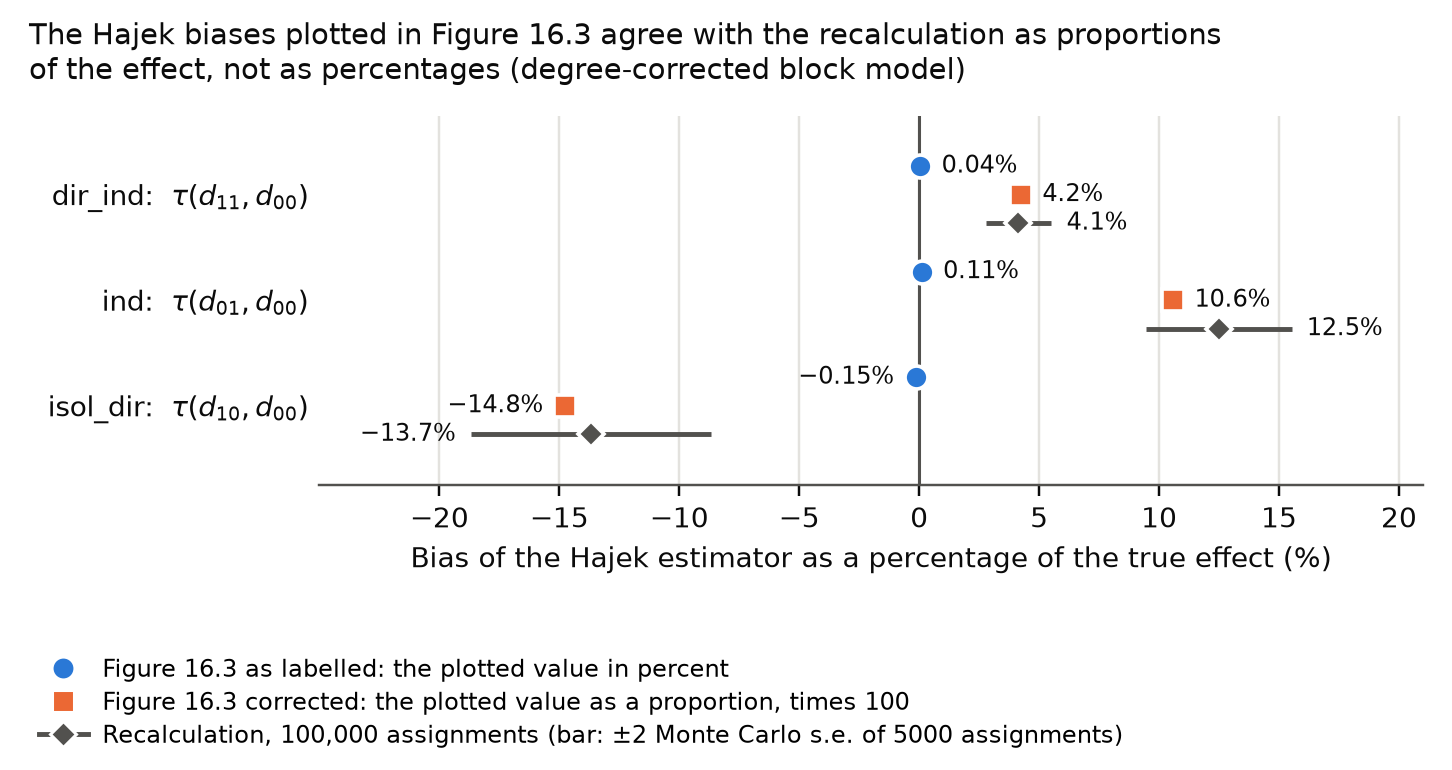
  • Page 212: when the exposure probabilities are exact and positive, the Horvitz–Thompson estimator is unbiased. The identity holds algebraically, and it holds when every assignment with two treated units on a cycle of six units is enumerated, with heterogeneous potential outcomes. With exposure probabilities simulated from 10,000 assignments and then held fixed, exact calculations on the regenerated degree-corrected block model give biases of about 0.5%0.5\%–1.5%1.5\% of the true effects. The conditions and the implementation are the subject of P044-E001, P044-E005 and P044-E006.
  • For the chapter’s control exposure and nonempty exposure groups, the function estimates() codes the Horvitz–Thompson totals, the Hajek means, the variance and covariance estimators with the correction for pairs of units whose joint exposure probability is zero, and the variance of a contrast as its documentation states. The Hajek variance calculation uses a linearized approximation. An independent implementation agrees with it to every printed digit on the regenerated observed assignment and on three other assignments. With exact probabilities, the expected Horvitz–Thompson variance estimates on the cycle of six units are at least the exact variances. The conservativeness of the Horvitz–Thompson variance estimators with simulated probabilities is the subject of P044-N005.
  • Page 218: the twelve numbers of the output for the degree-corrected block model (DCBM) are reproduced to their printed precision from the printed code and seeds, using the public source for version 0.5 of the package randnet.
  • Table 16.1: the 36 entries follow from the output on p. 218, with each standard error equal to the square root of the variance estimate and each tt-statistic equal to the estimate divided by its standard error. The entries are truncated to two decimals, not rounded. The tt-statistic is smaller for the DCBM in five of the six comparisons; the exception is the Horvitz–Thompson estimate for (d01,d00)(d_{01},d_{00}). The variance estimates are larger for the DCBM in all six comparisons.
  • Pages 213–214: the small-world generator gives 10001000 units and mean degree exactly 1010. Over 200 seeds its degree variance is about 1.91.9 and its skewness about 0.110.11, which is consistent with the printed 22 and 0.120.12. The DCBM that the printed code generates has mean degree 9.869.86, variance 75.8775.87 and skewness 1.0751.075. The description of that network is corrected in P044-E003, and the small-world graph from the printed seed is the subject of P044-N004.
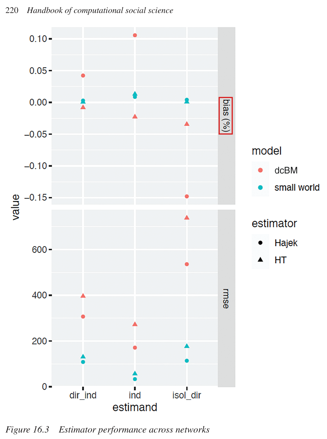
  • Figure 16.3, lower panel: in my 100,000-assignment DCBM recalculation, the root mean squared errors are 396, 269 and 771 for Horvitz–Thompson and 303, 168 and 554 for Hajek, in figure order (P044-N009). They are within about 5% of the values read from the figure. A separate 5,000-assignment calculation on a different small-world realization is also within about 5%. The Hajek estimator has the lower value in all six cells, and the values are larger for the DCBM in all six. The upper panel is the subject of P044-N009.
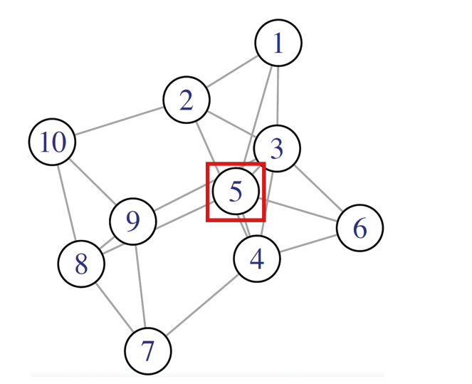
  • Figure 16.1 has 20 edges, and units 1 and 2 are both adjacent to unit 3, as p. 213 says. The list of the ties of unit 2 is corrected in P044-N003.
  • Every function call printed in the chapter is valid for the package, the default multipliers are (2,1.5,1.25)(2,1.5,1.25) in the stated order, and the printed construction of the observed outcomes implements the one described. Both network generators repeat until no unit is isolated, and neither regenerated network has an isolated unit, in agreement with Note 1.
  • The package contains functions for graph cluster randomization and for the estimators of Hudgens and Halloran (2008), as the section “Further reading” says. Its sampler for Bernoulli designs is the subject of P044-N014.
  • The 16 entries of the reference list are all cited in the text, and every citation in the text has an entry. The title of one entry is corrected in P044-N012.

My checks had the following limits. The code for the simulation behind Figure 16.3 and for Figures 16.1 and 16.2 was not available, and neither were the original networks. Approximate results for Figure 16.3 were recomputed from its description (P044-N010). The small-world half of the output on p. 218 and of Table 16.1 was not reproduced, since the printed generator and seed do not regenerate the printed results with R 4.4.2 and igraph 2.2.2 (P044-N004). The chapter does not state which version of randnet it used. I did not consult Aronow and Samii (2017), Aronow et al. (2021) or the other works cited. The formulas of the 2017 article were compared with the package only through the package’s own documentation of them. The chapter states no theorem on the consistency of the Hajek or weighted least squares estimators, and I did not establish one. The chapter has no appendix or supplement. Parts of the package that the chapter neither describes nor uses lie outside the audited work, among them the helpers for misspecified networks, the functions for two-stage designs, the vignettes, the help pages and the replication script for the 2017 article. Defects found there are not entered as corrections to the chapter. I have not established that the rest of the chapter is correct.

I distinguish the exact-probability Horvitz–Thompson guarantee from finite simulation error. Finite assignment simulation approximates an ideal calculation, as finite bootstrap resampling does, and the analogy is compatible with the counterexamples. Increasing the number of draws with suitable accuracy checks is a possible remedy; the effort depends on the relevant joint exposure probabilities. The two forty-unit calculations with 10,000 simulated assignments condition on distinct probability tables; neither establishes a universal draw threshold or an incorrect published numeric entry. Convergence with independent draws with replacement on a fixed finite design, with fixed outcomes and exposure mapping and positive marginal support, also supplies no finite-draw guarantee (P044-N005).

Headline claims and related corrections

  1. Design-based causal inference under interference combines an experimental design, a known network and a plausible exposure mapping to define and estimate average exposure effects τ(d,d′)\tau(d,d'), without requiring linearity, effect homogeneity or a parametric model of the outcome distribution.

    Introduction pp. 209–210 (PDF pp. 1–2); 'Network experimental setting' and 'Exposure mappings and causal effects', the four-exposure display and τ(d,d′)\tau(d,d'), pp. 210–212 (PDF pp. 2–4); Conclusion pp. 219, 221 (PDF pp. 11, 13). No numbered theorem.

    See P044-E001, P044-A003, P044-E007.

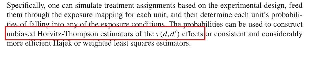
  2. Inverse weighting by exposure probabilities removes the confounding that arises from network position: Horvitz-Thompson estimators of τ(d,d′)\tau(d,d') are unbiased, and Hajek or weighted least squares estimators are consistent and considerably more efficient.

    'Design-based inference', p. 212 (PDF p. 4); p. 216 (PDF p. 8); Conclusion pp. 219, 221 (PDF pp. 11, 13); the make_exposure_prob and estimates() calls, pp. 216-218; Table 16.1.

    See P044-E001, P044-E005, P044-E006, P044-E008.

  3. Exposure probabilities can be computed from the design by simulating treatment assignments (here R=10,000R=10{,}000 draws of complete randomization with p=0.1p=0.1 and N=1000N=1000) and passing them through the exposure mapping; they then serve as generalized propensity scores.

    p. 212 (PDF p. 4); code blocks on pp. 214 and 216 (PDF pp. 6, 8); make_tr_vec_permutation(), make_exposure_prob().

    See P044-N005, P044-E005.

  4. Dependence in exposures through shared peers is handled by the Aronow-Samii sampling-theoretic variance estimators, which are conservative approximations to the exact variances; Table 16.1 reports the resulting standard errors and tt-statistics.

    p. 213 (PDF p. 5); p. 217 (PDF p. 9); Conclusion item (b), p. 221 (PDF p. 13); Figure 16.1; Table 16.1 s.e. and tt rows; console output on p. 218, including the Horvitz–Thompson and Hajek contrast-variance outputs.

    See P044-N005, P044-E005, P044-N003.

  5. In one simulated experiment on each network the estimated exposure effects, standard errors and tt-statistics are as in Table 16.1, and the tt-statistics are generally smaller for the DCBM.

    Table 16.1 (PDF p. 11, printed p. 219); console output on p. 218 (PDF p. 10).

    See P044-E003, P044-E002, P044-N004.

  6. Over 5000 re-randomizations, bias and RMSE are larger on the DCBM than on the small world, and the Hajek estimator's variance reduction outweighs its bias, so that it has substantially lower RMSE, most visibly on the DCBM.

    Figure 16.3 (PDF p. 12, printed p. 220); p. 219 (PDF p. 11).

    See P044-N009, P044-N010, P044-E002.

  7. Network topology affects precision and power: a network with a highly skewed degree distribution (the DCBM) gives much noisier estimates than one with a tight degree distribution (the small world), because skewed degrees produce skewed exposure probabilities; analysts should simulate experiments on networks resembling those they will study to assess power.

    Introduction pp. 209-210 (PDF pp. 1-2); Examples pp. 213-214 (PDF pp. 5-6); Conclusion p. 221 (PDF p. 13); Figure 16.2, Table 16.1, Figure 16.3.

    See P044-E002.

  8. The two example networks are described as a small world (N=1000N=1000, mean degree 10, rewiring probability 0.10, degree variance 2 and skewness 0.12) and a degree-corrected block model (N=1000N=1000, 10 communities assigned uniformly at random, expected within-community edge share 0.7, expected mean degree 10, degree variance 75 and skewness 1.07).

    pp. 213-214 (PDF pp. 5-6); Figure 16.2; code on p. 215 (PDF p. 7).

    See P044-E003, P044-N004.

  9. The interference R package implements these methods, and also offers graph cluster randomization and the Hudgens-Halloran estimators for partial interference.

    Introduction p. 209 (PDF p. 1); the worked code on pp. 213-219 (PDF pp. 5-11); 'Further reading', p. 221 (PDF p. 13); package source.

    See P044-E005, P044-E006, P044-E008, P044-N014.

  10. Because inferential properties are defined in terms of the experimental design, analysts can choose designs that control bias and improve efficiency in a way that is robust across application areas and outcome distributions.

    Introduction p. 209 (PDF p. 1), paragraph beginning 'Analysis of network experiments'; Table 16.1; Figure 16.3.

    See P044-E001, P044-E005.

Corrections

Major (1)

A central result, method or key claim fails for a non-trivial reason, and the repair changes what the paper establishes.

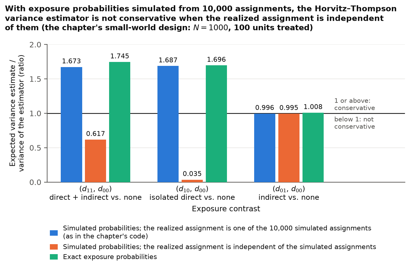
The Horvitz–Thompson variance estimator is conservative with exact exposure probabilities and positive marginal support, but not in general with probabilities simulated from 10,000 assignments, as in the chapter: in a small-world network regenerated from the printed code its expectation is 0.617, 0.035 and 0.995 times the variance of the estimator for the three contrasts when the realized assignment is independent of the simulated ones.

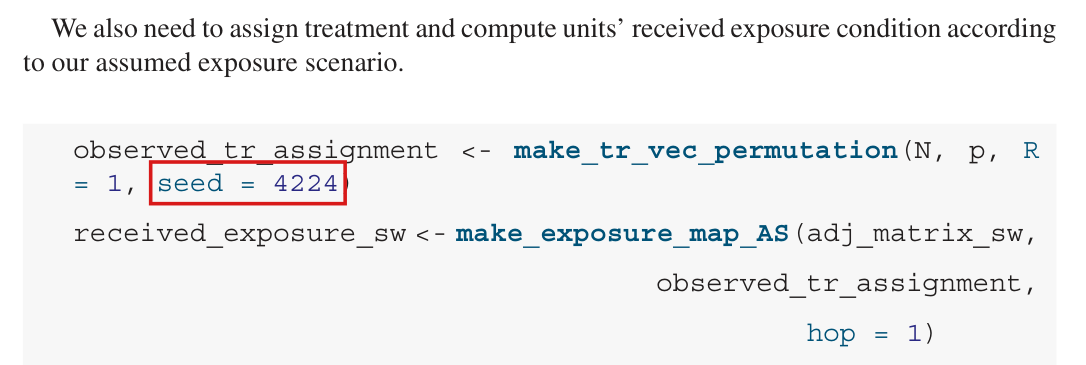
p. 217 (PDF p. 9), last paragraph, first sentence; the code lines with seed = 4224 on p. 214 (PDF p. 6) and p. 217

See also under Formal statements (Lean): P044-T1, P044-T2, P044-T11

I disputed this classification, but as a rule, deferred to the models’ final judgment: see my comment and the history of this entry.

As printed

p. 217: “Next, we estimate exposure-specific effects using both the Horvitz–Thompson and Hajek estimators, as well as the variance estimators of these effects, which are conservative approximations to the exact variances.”

p. 214, joined on one line:

possible_tr_assignment <- make_tr_vec_permutation(N, p, R = 10000, seed = 4224)

p. 217: “We also need to assign treatment and compute units' received exposure condition according to our assumed exposure scenario.”

observed_tr_assignment <- make_tr_vec_permutation(N, p, R = 1, seed = 4224)

The problem

Recall that a variance estimator is conservative if its expectation over the randomization is at least the variance of the effect estimator. The Horvitz–Thompson variance estimator has this property when it is computed with the exact exposure probabilities of the design and every unit has positive probability of both contrasted exposures. The chapter computes it with exposure probabilities simulated from R=10,000R=10{,}000 assignments, and the property does not carry over. The estimator divides by the simulated probability that two units are jointly in given exposures, and for rare joint exposures this frequency rests on few assignments. In the regenerated network, among pairs of units that are both in isolated direct exposure, the smallest positive count in the 10,000 simulated assignments is 1.

Finite simulation introduces numerical error here, just as a finite number of bootstrap resamples approximates the ideal bootstrap calculation. This familiar issue can be addressed by controlling simulation error; a draw count alone does not show that the resulting Horvitz–Thompson variance estimates remain conservative.

The worked example uses an assignment from the probability simulation. Both calls to make_tr_vec_permutation set the seed 4224, which implies that the realized assignment of p. 217 is the first of the 10,000 simulated assignments of p. 214. The text does not say so; it says “We also need to assign treatment”. In an experiment analyzed by this recipe, the realized assignment is ordinarily drawn independently of the simulated assignments. The two cases differ in the small-world network regenerated from the printed code. When the realized assignment is uniform among the simulated assignments, the expectation of the Horvitz–Thompson variance estimator is 1.673, 1.687 and 0.996 times the variance of the Horvitz–Thompson estimator for the contrasts (d11,d00)(d_{11},d_{00}), (d10,d00)(d_{10},d_{00}) and (d01,d00)(d_{01},d_{00}). When the realized assignment is independent of them, the expectation is 0.617, 0.035 and 0.995 times that variance, and the observed shares of negative variance estimates are 9%, 40% and 0%. Inclusion raises the first two ratios above 1 but leaves the third below 1. Applied to an experiment, the recipe can return a Horvitz–Thompson variance estimate that is a small fraction of the variance of the estimator, or negative. Exact counterexamples show that neither a large RR nor a realized assignment among the simulated ones guarantees that the estimator is conservative.

Evidence an exact counterexample

I checked the claim with a recalculation in the chapter’s small-world design, exact counterexamples and a derivation, supplemented by a second recorded 10,000-assignment table and a finite-bootstrap comparison.

The small-world design. The small-world network was regenerated with the printed code (N=1000N=1000, nei = 5, rewiring probability 0.1, seed 42), the 10,000 simulated assignments (100 of 1000 units treated, seed 4224) and the potential outcomes (seed 547). The package then computed the exposure probabilities. The regenerated network need not be the chapter’s realization: its degree variance is 1.87 and its skewness is 0.07, against 2 and 0.12 on p. 214. Conditional on the 10,000 simulated assignments, the expectation of each variance estimator and the variance of each effect estimator were computed under two distributions of the realized assignment. In the first, the realized assignment is uniform on the 10,000 simulated assignments. In the second, it is drawn by complete randomization, independently of them. For the Horvitz–Thompson estimator, both moments are exact sums over the joint exposure probabilities of the distribution in question, with an empty exposure sum defined as zero; the package instead returns an undefined value when an exposure group is absent. The shares of negative variance estimates, the coverage and the Hajek ratios use all 10,000 simulated assignments in the first case and are estimated from 30,000 independent assignments in the second; all evaluated assignments have all four exposure groups present.

Small-world design regenerated from the printed code (N=1000N=1000, 100 units treated, exposure probabilities simulated from R=10,000R=10{,}000 assignments). HT: Horvitz–Thompson. Ratio: expected variance estimate divided by the variance of the effect estimator, conditional on the simulated assignments. Negative: share of realized assignments under which the variance estimate is negative. Coverage: share under which the interval τ^HT±1.96 V^HT1/2\widehat\tau_{HT}\pm1.96\,\widehat V_{HT}^{1/2} contains the true effect; a negative V^HT\widehat V_{HT} counts as a miss. Independent-assignment negative shares, coverage and Hajek ratios are simulation estimates.
Realized assignmentContrastHT ratioHT negativeHT coverageHajek ratio
one of the simulated(d11,d00)(d_{11},d_{00})1.6730.00%97.9%1.824
one of the simulated(d10,d00)(d_{10},d_{00})1.6870.17%96.3%1.705
one of the simulated(d01,d00)(d_{01},d_{00})0.9960.00%94.9%1.006
independent(d11,d00)(d_{11},d_{00})0.6178.97%75.8%1.817
independent(d10,d00)(d_{10},d_{00})0.03540.06%44.4%1.824
independent(d01,d00)(d_{01},d_{00})0.9950.00%94.8%1.022

Averaging also over the simulated assignments by numerical integration, with a negligible bound on the approximation of sampling without replacement, the Horvitz–Thompson ratios are 1.664, 1.667 and 0.996 in the first case and 0.632, 0.072 and 0.980 in the second. With exact exposure probabilities the ratios are 1.745, 1.696 and 1.008. With exact marginal probabilities and simulated joint probabilities they are 0.648, 0.020 and 1.006 for an independent realized assignment. This shows that the shortfall persists with exact marginal probabilities. The ratios for the degree-corrected block model were not computed.

Exact counterexamples. In each, the exposure mapping is the chapter’s, treatment is by complete randomization, and every unit has positive probability of each of the four exposures. The contrast is (d01,d00)(d_{01},d_{00}). The simulated assignments are a uniform sample of distinct assignments, as make_tr_vec_permutation draws them, and the moments are exact rational numbers.

  1. Twelve units form three disjoint cliques of four, two units are treated, all potential outcomes equal 1, and the probabilities are simulated from 65 of the 66 assignments. Over all such samples, the variance of the Horvitz–Thompson estimator is 0.48766 and the expected variance estimate is 0.44710 when the realized assignment is independent of the sample. They are 0.48734 and 0.44874 when it is one of the 65. With exact probabilities both equal 6050/119076050/11907.
  2. Ten units form a cycle, two units are treated, yi(d00)=1y_i(d_{00})=1 and the other potential outcomes are 0, and the probabilities are simulated from 20 of the 45 assignments. Over all such samples, the expected variance estimate is −0.0711-0.0711 against a variance of 0.0370 when the realized assignment is independent of the sample, and 0.0173 against 0.0334 when it is one of the 20. With exact probabilities the expected variance estimate is 32/24532/245 and the variance is 3/983/98.
  3. Forty units form eight disjoint cliques of five, four units are treated, all potential outcomes equal 1, and the probabilities are simulated from one recorded sample of R=10,000R=10{,}000 of the 91,390 assignments. Given this sample, the expected variance estimate is 0.12980 against a variance of 0.13262 when the realized assignment is independent of the sample, and 0.13013 against 0.13036 when it is one of the 10,000.

For a second probability table for the same forty-unit design, using Python seed 20261019 for its 10,000 distinct assignments, I obtain an expected variance estimate of 0.1305278229990.130527822999 against variance 0.1326645198080.132664519808 for an independent realized assignment, and 0.1309072085150.130907208515 against 0.1311302097150.131130209715 when the realized assignment is included. Every positive relevant joint has a positive empirical count, with minimum 845; exact probabilities give equality at 7430620902683355/55988922226386688≈0.1327159124917430620902683355/55988922226386688\approx0.132715912491. These moments condition on this probability table rather than averaging over all 10,000-assignment samples. Both tables concern this forty-unit design rather than the chapter’s published networks, and neither calculation establishes a numerical error in a published table entry.

Finite simulation and accuracy. The literal bootstrap analogy concerns a computational approximation. For fixed observed data (0,1)(0,1), the ideal variance of a two-observation bootstrap mean is 1/81/8. With B≥2B\ge2 independent bootstrap means, their sample variance with denominator B−1B-1 has expectation 1/81/8, but is zero with probability 2(1/4)B+(1/2)B>02(1/4)^B+(1/2)^B>0; denominator BB gives expectation (B−1)/(8B)(B-1)/(8B). This illustrates finite computational error without equating its bias mechanism to the nonlinear Horvitz–Thompson plug-in or establishing bootstrap validity for an original sampling distribution.

The package samples distinct assignments by default. If MM assignments are possible and an exposure event has exact probability qq, its count CC in RR uniform draws without replacement is hypergeometric, with

E[C/R]=q,Var⁡(C/R)=q(1−q)RM−RM−1.\mathbb{E}[C/R]=q,\qquad \operatorname{Var}(C/R)=\frac{q(1-q)}R\frac{M-R}{M-1}.

Thus its relative standard deviation depends on RqRq, not on RR alone. At R=10,000R=10{,}000 and negligible sampling fraction, the illustrative probabilities .01.01, .001.001 and .0001.0001 give relative standard deviations about .0995.0995, .3161.3161 and .9999.9999; these are not measurements of the chapter’s graph. The routine also uses (Ci+1)/(R+1)(C_i+1)/(R+1) for marginals, Cij/(R+1)C_{ij}/(R+1) for same-exposure off-diagonal joints and Cij/RC_{ij}/R for cross-exposure joints. Smoothing and these distinct normalizers must be included in an accuracy argument, along with support and zero-count handling. A bound holding with high probability does not alone prove conservative expectation without control of the failure event and any needed margin or inflation.

For independent with-replacement simulation from a fixed finite design, fixed finite outcomes and mapping, positive contrast marginals and finitely many relevant positive joints, the strong law and vanishing smoothing give almost-sure convergence of the coefficient formulas and their fixed-design conditional moments to their exact-probability counterparts once support is correctly distinguished. This is no finite-RR inequality, no uniform guarantee over changing designs or shrinking positive joints, no growing-NN result, and no coverage guarantee. For the default without-replacement scheme, R≤MR\le M at fixed design; even a full census retains the routine’s R+1R+1 smoothing. Analytic probabilities or unsmoothed census frequencies are exact alternatives. Sufficiently accurate simulation with justified error accounting can also be adequate.

Derivation for exact probabilities. Let πi(d)=Pr⁡(Di=d)\pi_i(d)=\Pr(D_i=d) and πij(d,d′)=Pr⁡(Di=d, Dj=d′)\pi_{ij}(d,d')=\Pr(D_i=d,\,D_j=d'), with πii(d,d)=πi(d)\pi_{ii}(d,d)=\pi_i(d), and write Ii(d)=1{Di=d}I_i(d)=\mathbf{1}\{D_i=d\} and Yi=yi(Di)Y_i=y_i(D_i). The Horvitz–Thompson estimator of the total under dd is T^d=∑iIi(d) Yi/πi(d)\widehat T_d=\sum_i I_i(d)\,Y_i/\pi_i(d), and τ^HT(d,d′)=(T^d−T^d′)/N\widehat\tau_{HT}(d,d')=(\widehat T_d-\widehat T_{d'})/N. The variance estimator is V^HT(d,d′)=N−2(W^d+W^d′−2 C^dd′)\widehat V_{HT}(d,d')=N^{-2}\bigl(\widehat W_d+\widehat W_{d'}-2\,\widehat C_{dd'}\bigr), where

W^d=∑i,j: πij(d,d)>0Ii(d) Ij(d) πij(d,d)−πi(d)πj(d)πij(d,d) YiYjπi(d)πj(d)+∑i≠j: πij(d,d)=0(Ii(d) Yi22πi(d)+Ij(d) Yj22πj(d)),C^dd′=∑i,j: πij(d,d′)>0Ii(d) Ij(d′) πij(d,d′)−πi(d)πj(d′)πij(d,d′) YiYjπi(d)πj(d′)−∑i,j: πij(d,d′)=0(Ii(d) Yi22πi(d)+Ij(d′) Yj22πj(d′)).\begin{aligned} \widehat W_d={}&\sum_{i,j:\,\pi_{ij}(d,d)>0}I_i(d)\,I_j(d)\,\frac{\pi_{ij}(d,d)-\pi_i(d)\pi_j(d)}{\pi_{ij}(d,d)}\,\frac{Y_iY_j}{\pi_i(d)\pi_j(d)}\\ &+\sum_{i\neq j:\,\pi_{ij}(d,d)=0}\Bigl(\frac{I_i(d)\,Y_i^2}{2\pi_i(d)}+\frac{I_j(d)\,Y_j^2}{2\pi_j(d)}\Bigr),\\ \widehat C_{dd'}={}&\sum_{i,j:\,\pi_{ij}(d,d')>0}I_i(d)\,I_j(d')\,\frac{\pi_{ij}(d,d')-\pi_i(d)\pi_j(d')}{\pi_{ij}(d,d')}\,\frac{Y_iY_j}{\pi_i(d)\pi_j(d')}\\ &-\sum_{i,j:\,\pi_{ij}(d,d')=0}\Bigl(\frac{I_i(d)\,Y_i^2}{2\pi_i(d)}+\frac{I_j(d')\,Y_j^2}{2\pi_j(d')}\Bigr). \end{aligned}

Each term of the two sums over positive joint probabilities has expectation equal to the corresponding term of Var⁡(T^d)\operatorname{Var}(\widehat T_d) or of Cov⁡(T^d,T^d′)\operatorname{Cov}(\widehat T_d,\widehat T_{d'}). For a pair with πij(d,d)=0\pi_{ij}(d,d)=0, the term of the variance is −yi(d) yj(d)-y_i(d)\,y_j(d), and the second sum of W^d\widehat W_d has expectation (yi(d)2+yj(d)2)/2\bigl(y_i(d)^2+y_j(d)^2\bigr)/2 for that pair. For a pair with πij(d,d′)=0\pi_{ij}(d,d')=0, the term of the covariance is −yi(d) yj(d′)-y_i(d)\,y_j(d'), and the second sum of C^dd′\widehat C_{dd'} has expectation −(yi(d)2+yj(d′)2)/2-\bigl(y_i(d)^2+y_j(d')^2\bigr)/2. Collecting terms gives

E[V^HT(d,d′)]−Var⁡(τ^HT(d,d′))=12N2∑i≠j: πij(d,d)=0(yi(d)+yj(d))2+12N2∑i≠j: πij(d′,d′)=0(yi(d′)+yj(d′))2+1N2∑i,j: πij(d,d′)=0(yi(d)−yj(d′))2  ≥  0.\begin{aligned} \mathbb{E}\bigl[\widehat V_{HT}(d,d')\bigr]-\operatorname{Var}\bigl(\widehat\tau_{HT}(d,d')\bigr)={}&\frac{1}{2N^2}\sum_{i\neq j:\,\pi_{ij}(d,d)=0}\bigl(y_i(d)+y_j(d)\bigr)^2\\ &+\frac{1}{2N^2}\sum_{i\neq j:\,\pi_{ij}(d',d')=0}\bigl(y_i(d')+y_j(d')\bigr)^2\\ &+\frac{1}{N^2}\sum_{i,j:\,\pi_{ij}(d,d')=0}\bigl(y_i(d)-y_j(d')\bigr)^2\;\ge\;0. \end{aligned}

The first step of this computation uses that the probabilities inside V^HT\widehat V_{HT} are those of the distribution of the realized assignment. With simulated probabilities in their place the identity fails, as the counterexamples show.

What survives

The exposure mapping, the estimands and the Horvitz–Thompson variance estimator computed with exact exposure probabilities under positive marginal support are unaffected. No entry of Table 16.1 is shown to be wrong. Its Horvitz–Thompson standard errors and tt-statistics were computed with the realized assignment among the simulated assignments, and they describe that case. Figure 16.3 reports the bias and the RMSE of the point estimators and does not depend on the variance estimators. In the regenerated small-world design, the Hajek variance ratios are approximately between 1.01 and 1.82 in the first case and are estimated to lie approximately between 1.02 and 1.82 in the independent case. These results concern that design and give no general guarantee. What is lost is the assurance that the Horvitz–Thompson variance estimator computed with simulated exposure probabilities is conservative.

Corrected

Next, the exposure-specific effects are estimated using both the Horvitz–Thompson and Hajek estimators, together with variance estimators of these effects. Let πi(d)\pi_i(d) and πij(d,d′)\pi_{ij}(d,d') be the exact exposure probabilities of the design, and suppose that πi(d)>0\pi_i(d)>0 and πi(d′)>0\pi_i(d')>0 for every unit ii. Then the Horvitz–Thompson variance estimator V^HT(d,d′)\widehat V_{HT}(d,d') computed with these probabilities, including its terms for pairs of units with joint exposure probability zero, is conservative:

E[V^HT(d,d′)]  ≥  Var⁡(τ^HT(d,d′)).\mathbb{E}\bigl[\widehat V_{HT}(d,d')\bigr]\;\ge\;\operatorname{Var}\bigl(\widehat\tau_{HT}(d,d')\bigr).

The exposure probabilities used below are simulated from R=10,000R=10{,}000 assignments, and the variance estimator computed from them need not be conservative, even at R=10,000R=10{,}000 and even if the realized assignment is one of the simulated assignments, as it is in the code below, where both calls use seed 4224. Exact probabilities retain this variance guarantee; a method using simulated probabilities needs a separate justification that accounts for their simulation error. Increasing the number of assignments with suitable accuracy checks is one possible computational remedy; the necessary effort depends on the joint exposure probabilities relevant to the contrasts. This expectation guarantee alone does not guarantee confidence-interval coverage. The Hajek variance estimator is a linearized approximation and has no general finite-sample guarantee.

For the design of the examples the exact probabilities have closed forms. Under complete randomization of mm of NN units, the probability that oo given units are treated and ff other given units are not is Q(o,f)=(N−o−fm−o)/(Nm)Q(o,f)=\binom{N-o-f}{m-o}\big/\binom{N}{m}. For a unit with gig_i neighbors, πi(d10)=Q(1,gi)\pi_i(d_{10})=Q(1,g_i), πi(d00)=Q(0,gi+1)\pi_i(d_{00})=Q(0,g_i+1), πi(d11)=m/N−Q(1,gi)\pi_i(d_{11})=m/N-Q(1,g_i) and πi(d01)=(N−m)/N−Q(0,gi+1)\pi_i(d_{01})=(N-m)/N-Q(0,g_i+1). The joint probabilities follow in the same way by inclusion and exclusion over the two neighbor sets.

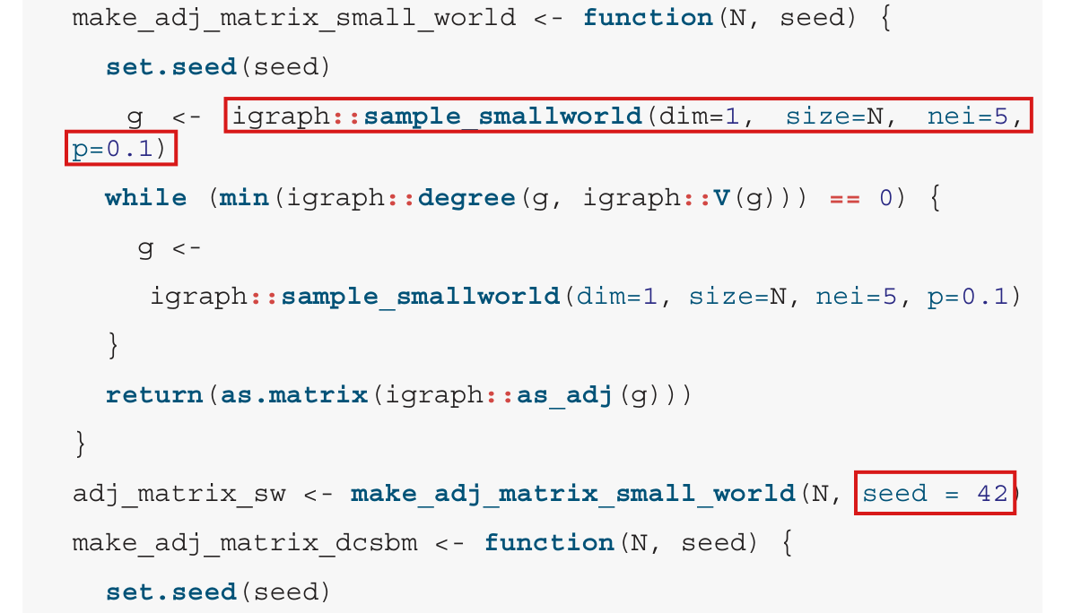
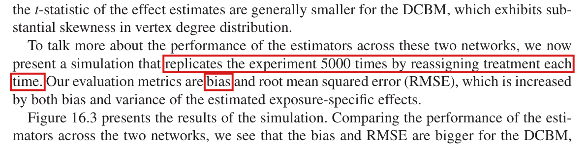
Crop of five lines of text beginning 'Next, we estimate exposure-specific effects using both the Horvitz-Thompson and Hajek estimators, as well as the variance estimators of these effects'. Two red boxes mark the words 'which are conservative approximations to the exact variances.'
p. 217 (PDF p. 9), last paragraph, first sentence. The marked clause calls the variance estimators conservative.
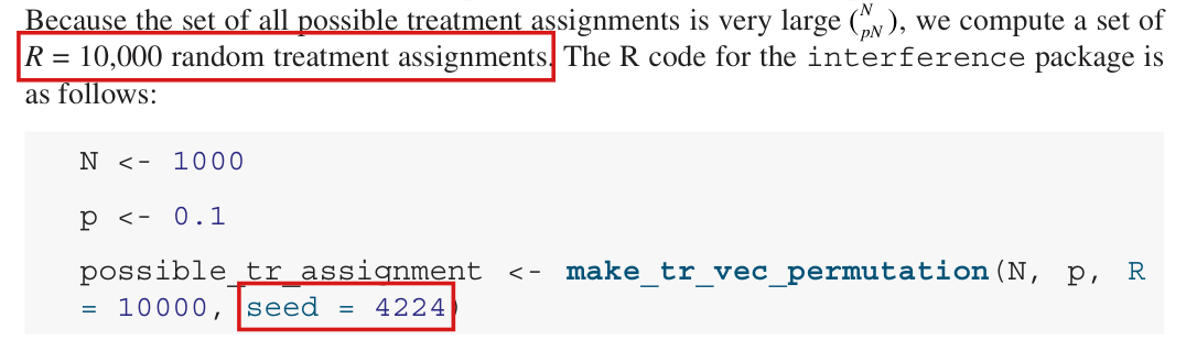
Crop of three lines of text and a code listing. A red box marks the words 'R = 10,000 random treatment assignments.' The code reads N <- 1000, p <- 0.1, possible_tr_assignment <- make_tr_vec_permutation(N, p, R = 10000, seed = 4224), and a second red box marks 'seed = 4224'.
p. 214 (PDF p. 6): the 10,000 simulated assignments from which the exposure probabilities are computed. The marked seed is used again on p. 217.
Crop of the sentence 'We also need to assign treatment and compute units' received exposure condition according to our assumed exposure scenario.' and a code listing that begins observed_tr_assignment <- make_tr_vec_permutation(N, p, R = 1, seed = 4224). A red box marks 'seed = 4224'.
p. 217 (PDF p. 9): the realized assignment. With the marked seed it is the first of the 10,000 simulated assignments of p. 214.
Bar chart with three groups of three bars, one group for each contrast, and a horizontal line at the ratio 1. For the contrast (d11, d00) the bars are 1.673 with simulated probabilities and the realized assignment among the simulated assignments, 0.617 with simulated probabilities and an independent realized assignment, and 1.745 with exact probabilities. For (d10, d00) they are 1.687, 0.035 and 1.696. For (d01, d00) they are 0.996, 0.995 and 1.008.
Expected Horvitz–Thompson variance estimate divided by the variance of the Horvitz–Thompson estimator, for the three contrasts in the small-world design regenerated from the printed code (N=1000N=1000, 100 units treated). The blue and orange bars use probabilities simulated from R=10,000R=10{,}000 assignments and condition on those assignments; the green bars use exact probabilities. A value below 1 means that the variance estimator is not conservative.
My comment and the history of this entry

I agree that this is an important practical problem. I think there's a bit of ambiguity in wording (the estimator is conservative, the Monte Carlo-based approximation doesn't have enough replicates in some applications). I think the answer is "K=10000" replicates is not sufficient for some applications, or some correction is needed to guarantee conservatism. This is not an unfamiliar problem (think, e.g., the bootstrap).

Comment after LLM decision: I don't know if I agree that this is a major error per se, but I do agree that it should be flagged, and I'm glad that this is getting attention.

Suggested classification: Moderate error.

My position My comment above; I suggested a Moderate error.

The models’ position The Horvitz–Thompson variance estimator is conservative with exact exposure probabilities and positive marginal support. In a small-world network regenerated from the chapter’s printed code, the finite simulation recipe can severely understate variance when the realized assignment is independent of the simulated assignments, which undermines a central guarantee of conservativeness: Major. No published table entry is shown to be wrong.

  1. Classification before my review (the classification when the audit was first completed, before I reviewed it): Major error.
  2. I commented and suggested a Moderate error.
  3. Independent evaluation. Incorporated in part. The entry now gives the analogy with the bootstrap and names more simulation draws, with accuracy checks or proved error control, as a possible remedy. My suggested rating (Moderate) was not adopted.

Moderate (1)

A real substantive error with limited reach.

The rows returned by the Bernoulli samplers of the interference package are not independent draws from the Bernoulli design, because the samplers discard every proposed profile that equals an earlier row; to simulate that design, repeated profiles must be kept.

Section “Network experimental setting”, p. 210 (PDF p. 2), definition of the Bernoulli design; Section “Design-based inference”, p. 212 (PDF p. 4), recipe for exposure probabilities; package interference, file R/make_tr_vec_bernoulli.R, lines 179–187 and 117–152

As printed

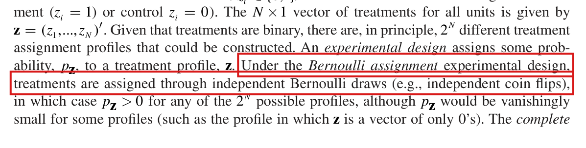
Chapter, p. 210: “Under the Bernoulli assignment experimental design, treatments are assigned through independent Bernoulli draws (e.g., independent coin flips), in which case pz>0p_{\mathbf{z}}>0 for any of the 2N2^N possible profiles, although pzp_{\mathbf{z}} would be vanishingly small for some profiles (such as the profile in which z\mathbf{z} is a vector of only 0’s).”

Chapter, p. 212: “Specifically, one can simulate treatment assignments based on the experimental design, feed them through the exposure mapping for each unit, and then determine each unit’s probabilities of falling into any of the exposure conditions.”

Package interference, file R/make_tr_vec_bernoulli.R, documentation, lines 10–11 and 13: “Sampling of treatment vectors is without replacement.” “@param p probability that treatment takes the value 1.”

The same file, lines 180–186, inside the loop for (i in 1:R) (indentation and one blank line removed):

vec <- rbinom(N, 1, p)

while (any(duplicated(rbind(vec, tr_vec_sampled[1:i - 1,]))))

{

vec <- rbinom(N, 1, p)

}

tr_vec_sampled[i,] <- vec

The problem

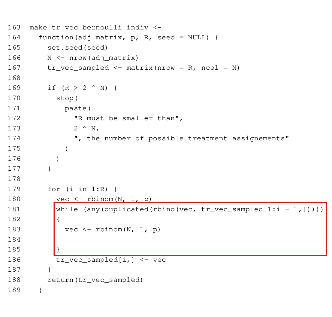
The chapter defines the Bernoulli design and gives a recipe for exposure probabilities: simulate assignments from the design, and count how often each unit falls in each exposure condition. Independent draws suffice, but dependent rows with the right marginal law or suitable sampling weights can also yield unbiased estimates. The function make_tr_vec_bernoulli of the package does not generally preserve that marginal law. A proposed profile that equals an earlier row is discarded and drawn again, both in the unit-level sampler (lines 181–185) and in the cluster sampler (lines 117–152).

Let q(z)=p∑izi(1−p)N−∑iziq(\mathbf{z})=p^{\sum_i z_i}(1-p)^{N-\sum_i z_i} be the probability of the profile z\mathbf{z} under the unit-level design, and let SS be the set of rows already accepted, with q(S)=∑s∈Sq(s)q(S)=\sum_{\mathbf{s}\in S}q(\mathbf{s}). While q(S)<1q(S)<1, the next row to be accepted equals a profile z∉S\mathbf{z}\notin S with probability q(z)/(1−q(S))q(\mathbf{z})/(1-q(S)), and it never equals a member of SS. The first row has the law qq; later rows are conditioned to exclude earlier profiles. The routine make_exposure_prob weights the returned rows equally. This can overrepresent low-probability profiles and distort exposure probabilities. Inverse probability weights and variance estimates that use the distorted probabilities can be affected, and the package gives no warning. The documentation says correctly that sampling is without replacement; it does not explain that the returned rows need not retain the design’s marginal law with parameter p.

The distortion is not confined to small examples. Among distinct profiles, at most one has no treated unit and at most NN have exactly one treated unit. With N=100N=100, p=0.01p=0.01 and R=1000R=1000, at least 899899 of the returned rows have two or more treated units, and the rows contain at least 100+2⋅899=1898100+2\cdot 899=1898 treated entries among 100,000100{,}000. The treatment frequency is at least 0.018980.01898, where the design has 0.010.01. When repeated profiles are unlikely over the RR draws, the loop usually has no effect.

Evidence an exact counterexample

I checked the counterexample in exact rational arithmetic and by running the unmodified package functions. Since each proposal has the law qq, for z∉S\mathbf{z}\notin S and q(S)<1q(S)<1 the probability that z\mathbf{z} is the next row to be accepted is

∑m=0∞q(S)mq(z)=q(z)1−q(S).\sum_{m=0}^{\infty}q(S)^m q(\mathbf{z})=\frac{q(\mathbf{z})}{1-q(S)} .

Let the network consist of two units joined by an edge, so that neither is an isolate, and let p=1/5p=1/5. The profiles (0,0)(0,0), (0,1)(0,1), (1,0)(1,0) and (1,1)(1,1) have probabilities 16/2516/25, 4/254/25, 4/254/25 and 1/251/25, and they place unit 1 in the conditions no, ind1, isol_dir and dir_ind1, respectively. With R=4R=4, the largest value that the function accepts when N=2N=2, each profile is returned exactly once. The routine make_exposure_prob reports the marginal probability of a condition as (C+1)/(R+1)(C+1)/(R+1), where CC is the number of rows that place the unit in the condition.

Unit 1 in the two-unit network with p=1/5p=1/5 and R=4R=4: probability of each exposure condition under the Bernoulli design, frequency among the four returned rows, and value reported by make_exposure_prob.
ConditionDesignFrequency in rowsReported
dir_ind11/251/251/41/42/52/5
isol_dir4/254/251/41/42/52/5
ind14/254/251/41/42/52/5
no16/2516/251/41/42/52/5

For two different conditions, the routine reports the plain frequency. The reported probability that unit 1 is in isol_dir and unit 2 is in ind1 equals 1/41/4, where the design has 4/254/25. Since no adjustment enters this entry, the difference comes from the discarded repeats alone.

With R=2R=2 on the same network, there are fewer rows than profiles. In the first row, unit 1 is treated with probability 1/51/5. Conditioning on the first row, which is (0,0)(0,0), (0,1)(0,1), (1,0)(1,0) or (1,1)(1,1), I obtain for the second row

Pr⁡(Z2,1=1)=1625⋅5/259/25+425⋅5/2521/25+425⋅1/2521/25+125⋅4/2524/25=257630.\Pr(Z_{2,1}=1)=\frac{16}{25}\cdot\frac{5/25}{9/25}+\frac{4}{25}\cdot\frac{5/25}{21/25}+\frac{4}{25}\cdot\frac{1/25}{21/25}+\frac{1}{25}\cdot\frac{4/25}{24/25}=\frac{257}{630} .

For the expected frequency of treatment of unit 1 over the two rows, I find (1/5+257/630)/2=383/1260(1/5+257/630)/2=383/1260, where the design has 1/51/5. The cluster sampler puts both units of this network in one cluster. With R=2R=2, it must return (0,0)(0,0) and (1,1)(1,1) once each. The condition dir_ind1 then has frequency 1/21/2, where the design has 1/51/5. With a single unit, p=1/5p=1/5 and R=2R=2, the function returns one 00 and one 11, and the unit is treated in the second row with probability 4/54/5.

What survives

This defect does not alter the chapter’s definition of the Bernoulli design, its exposure mappings or its design-based identities when the exposure probabilities are those of the design. The worked example summarized in Table 16.1 uses the function make_tr_vec_permutation, which carries out complete random assignment, and the simulation in Figure 16.3 continues that design. Under a design that is uniform on its support, each row remains marginally uniform when repeats are discarded, so this point does not implicate those results. A single row (R=1R=1) from either Bernoulli sampler is unaffected by duplicate rejection. What can change is the calculation of exposure probabilities from several rows of make_tr_vec_bernoulli under a nonuniform design, with the weights and variance estimates that use them.

Corrected

In the unit-level sampler I delete the while loop of lines 181–185, and each row is one fresh draw:

for (i in 1:R) {

vec <- rbinom(N, 1, p)

tr_vec_sampled[i,] <- vec

}

I delete the loop of lines 117–152 in the cluster sampler in the same way, so that each row is one fresh clustering with one fresh draw for each cluster. The tests that stop the function when R exceeds the number of possible assignments are then unnecessary and are also deleted, along with the corresponding restriction in the documentation. The documentation reads “Sampling of treatment vectors is with replacement.”

With this change the rows are independent draws from the design, and the frequency of an exposure condition among them is an unbiased estimate of its probability π\pi. The adjustment in make_exposure_prob is a separate matter and remains: the reported value (C+1)/(R+1)(C+1)/(R+1) has expectation (Rπ+1)/(R+1)(R\pi+1)/(R+1). If instead every profile in the support is enumerated, each profile must enter with its probability q(z)q(\mathbf{z}); in the two-unit example this weighting returns 1/251/25, 4/254/25, 4/254/25 and 16/2516/25.

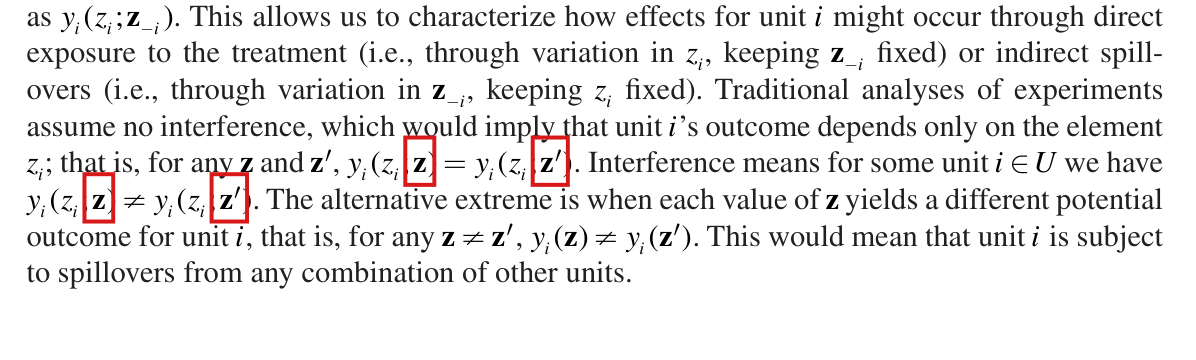
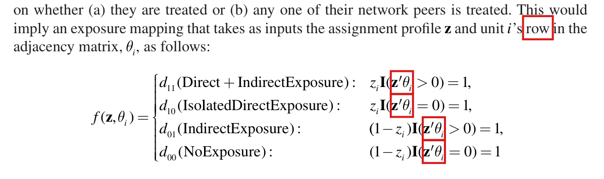
Crop of the Bernoulli-design definition and surrounding text. Red boxes mark the words 'Under the Bernoulli assignment experimental design, treatments are assigned through independent Bernoulli draws (e.g., independent coin flips),' which run over two lines.
Section “Network experimental setting”, p. 210 (PDF p. 2). The marked words define the Bernoulli design, which the package’s sampler is meant to simulate; the definition itself is correct.
Listing of lines 163 to 189 in monospaced type with line numbers: the function make_tr_vec_bernoulli_indiv. A red box marks lines 181 to 185, a while loop whose condition is any(duplicated(rbind(vec, tr_vec_sampled[1:i - 1,]))) and whose body assigns a new draw rbinom(N, 1, p) to vec. Above it, lines 169 to 177 stop the function if R exceeds 2 to the power N.
Package interference, file R/make_tr_vec_bernoulli.R, lines 163–189, typeset from the source file with line numbers added. The marked loop draws a new profile whenever the proposed one equals an earlier row.

Minor (12)

Real but inconsequential, for example a misprint that does not change a result.

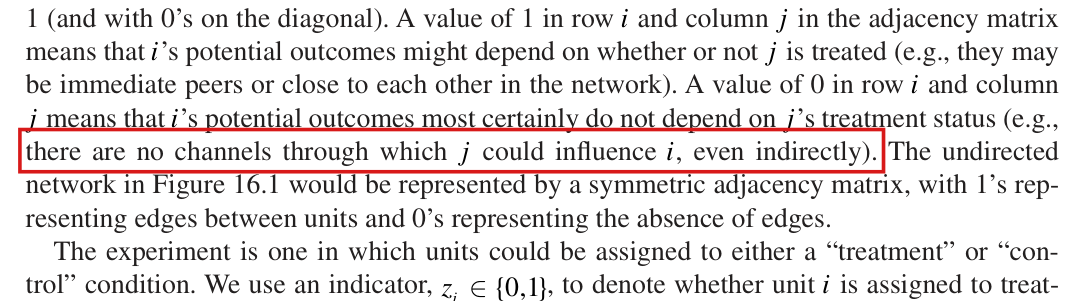
The Horvitz–Thompson estimator of the population contrast τ(d,d′)\tau(d,d') is unbiased only if every unit has positive probability of each of the two exposures dd and d′d' under the design; the chapter does not state this condition, and neither random assignment nor the absence of isolates guarantees it.

Section “Design-based inference”, p. 212 (PDF p. 4), last sentence; Section “Examples”, p. 216 (PDF p. 8), paragraph beginning “We now estimate exposure-specific effects”; Note 1, p. 221 (PDF p. 13)

See also under Formal statements (Lean): P044-T3, P044-T4, P044-T12

As printed

p. 212: “The probabilities can be used to construct unbiased Horvitz-Thompson estimators of the τ(d,d′)\tau(d,d') effects or consistent and considerably more efficient Hajek or weighted least squares estimators.”

p. 216: “This is precisely what inverse probability estimators like the Horvitz–Thompson take into account and the reason why we can obtain unbiased estimates of average potential outcomes in a specific exposure condition, and unbiased estimates of contrasts between these averages across different exposures.”

Note 1, p. 221: “Our networks do not have isolates, but we suggest researchers remove isolates from their analysis.”

The problem

The chapter defines the effect τ(d,d′)=N−1∑i=1N(yi(d)−yi(d′))\tau(d,d')=N^{-1}\sum_{i=1}^N(y_i(d)-y_i(d')) as an average over the whole population, and it says on p. 212 that the exposure probabilities give unbiased Horvitz–Thompson estimators of it. This holds only under a condition that the chapter does not state. Let πi(d)=Pr⁡(f(Z,θi)=d)\pi_i(d)=\Pr(f(\mathbf{Z},\theta_i)=d) be the probability that unit ii receives exposure dd under the design. The condition is that πi(d)>0\pi_i(d)>0 and πi(d′)>0\pi_i(d')>0 for every unit ii. If πj(d)=0\pi_j(d)=0 for some unit jj, then yj(d)y_j(d) is never observed. It can be changed without changing the distribution of anything that is observed, while τ(d,d′)\tau(d,d') changes with it. In that case no estimator is unbiased for τ(d,d′)\tau(d,d') over all potential outcomes, whatever weights it uses.

Random assignment does not guarantee the condition: there exist networks and designs such that some unit has probability zero of an exposure. Under complete random assignment, for example, a unit with enough peers cannot have all of them untreated. The only related guidance in the chapter is Note 1, which recommends that isolates be removed. The note does not claim that this is sufficient, and it is not sufficient: the example below has no isolates. The sentence on p. 216 needs the same condition when it is read as a general rule. The condition is the usual proviso of the Horvitz–Thompson result. The error is that the chapter states the result in general without it.

Evidence an exact counterexample

The evidence is an exact counterexample, obtained by enumerating all assignments in rational arithmetic, and a derivation of the corrected statement. I consider four units in a star: unit 1 is joined to units 2, 3 and 4, and there are no other edges. The degrees are (3,1,1,1)(3,1,1,1), so no unit is an isolate. Exactly two units are treated, chosen uniformly from the six pairs. This is complete random assignment with N=4N=4 and N1=2N_1=2. Under the chapter’s mapping with four conditions, the exposure probabilities are as follows.

Exposure probabilities in the four-unit star when exactly two units are treated uniformly at random, by exact enumeration of the six assignments.
Unitπi(d11)\pi_i(d_{11})πi(d10)\pi_i(d_{10})πi(d01)\pi_i(d_{01})πi(d00)\pi_i(d_{00})
1 (centre, degree 3)1/21/2001/21/200
2, 3 and 4 (leaves, degree 1)1/61/61/31/31/31/31/61/6

Unit 1 never receives d10d_{10} or d00d_{00}. Indeed, if it is treated, then one of its peers is treated, and if it is untreated, then two of its peers are treated. I compare two schedules of potential outcomes. In the first, yi(d)=1y_i(d)=1 for every unit and every exposure. The second differs from the first only in that y1(d00)=5y_1(d_{00})=5. Under each of the six assignments, the observed outcomes are (1,1,1,1)(1,1,1,1) in both schedules. The joint distribution of assignments, exposures and outcomes is then the same in both, and any estimator has the same expectation under both. However, τ(d11,d00)=0\tau(d_{11},d_{00})=0 in the first schedule and τ(d11,d00)=(1−5)/4=−1\tau(d_{11},d_{00})=(1-5)/4=-1 in the second. No estimator is unbiased under both. If each inverse-weighted sum is taken over the units observed in the exposure and divided by N=4N=4, then the expected contrast is 1−3/4=1/41-3/4=1/4 under both schedules. The bias is 1/41/4 in the first schedule and 5/45/4 in the second.

Under the condition, the estimator is unbiased. Let Di=f(Z,θi)D_i=f(\mathbf{Z},\theta_i), and let τ^HT(d,d′)\widehat\tau_{HT}(d,d') be the difference between the averages over ii of 1(Di=d) Yi/πi(d)\mathbf{1}(D_i=d)\,Y_i/\pi_i(d) and of 1(Di=d′) Yi/πi(d′)\mathbf{1}(D_i=d')\,Y_i/\pi_i(d'). Since Yi=yi(d)Y_i=y_i(d) on the event Di=dD_i=d and E[1(Di=d)]=πi(d)\mathbb{E}[\mathbf{1}(D_i=d)]=\pi_i(d), I have

E[1(Di=d) Yiπi(d)]=yi(d)πi(d) πi(d)=yi(d).\mathbb{E}\left[\frac{\mathbf{1}(D_i=d)\,Y_i}{\pi_i(d)}\right]=\frac{y_i(d)}{\pi_i(d)}\,\pi_i(d)=y_i(d).

Averaging over ii and subtracting the same identity for d′d', I obtain E[τ^HT(d,d′)]=τ(d,d′)\mathbb{E}[\widehat\tau_{HT}(d,d')]=\tau(d,d'). No condition on joint exposure probabilities, and no independence across units, is used.

For complete random assignment of MM of NN units and the mapping with four conditions, a unit with kk peers has

πi(d00)=(N−1−kM)/(NM),πi(d10)=(N−1−kM−1)/(NM),\pi_i(d_{00})=\binom{N-1-k}{M}\Big/\binom{N}{M},\qquad \pi_i(d_{10})=\binom{N-1-k}{M-1}\Big/\binom{N}{M},

where a binomial coefficient is zero when its lower index is negative or exceeds its upper index. For 2≤M≤N−12\le M\le N-1, all four exposures have positive probability exactly when 1≤k≤N−M−11\le k\le N-M-1. If isolates are removed, the lower end of this range is secured, and the upper end is not. In the star, N=4N=4, M=2M=2 and k=3k=3 for the centre. In the chapter’s design, N=1000N=1000 and M=100M=100, and the range is 1≤k≤8991\le k\le 899.

What survives

The exposure mapping and the estimand are well defined, and the Horvitz–Thompson estimator is unbiased wherever the condition holds. This counterexample does not establish an error in the estimates, the simulation or the comparison of precision for the two example networks. The degrees displayed in Figure 16.2 are compatible with the range 1≤k≤8991\le k\le 899, and no failure of the condition is established for either network. Note 1 is not itself incorrect. What changes is the general statement on p. 212, and the sentence on p. 216 when it is read as a general rule. An application in which some unit has probability zero of one of the two exposures must change the design or the target.

Corrected

p. 212: “Suppose that every unit ii in the population has positive probability of each of the two exposures being contrasted, that is, Pr⁡(f(Z,θi)=d)>0\Pr(f(\mathbf{Z},\theta_i)=d)>0 and Pr⁡(f(Z,θi)=d′)>0\Pr(f(\mathbf{Z},\theta_i)=d')>0 under the experimental design and the exposure mapping. The probabilities can then be used to construct unbiased Horvitz-Thompson estimators of the τ(d,d′)\tau(d,d') effects.”

In full, let the exposure mapping be correctly specified, so that Yi=yi(Di)Y_i=y_i(D_i) with Di=f(Z,θi)D_i=f(\mathbf{Z},\theta_i), and let πi(e)=Pr⁡(Di=e)\pi_i(e)=\Pr(D_i=e) be the exact exposure probabilities under the design. Suppose that πi(d)>0\pi_i(d)>0 and πi(d′)>0\pi_i(d')>0 for every i∈Ui\in U. Then the estimator

τ^HT(d,d′)=1N∑i=1N[1(Di=d) Yiπi(d)−1(Di=d′) Yiπi(d′)]\widehat\tau_{HT}(d,d')=\frac{1}{N}\sum_{i=1}^N\left[\frac{\mathbf{1}(D_i=d)\,Y_i}{\pi_i(d)}-\frac{\mathbf{1}(D_i=d')\,Y_i}{\pi_i(d')}\right]

satisfies E[τ^HT(d,d′)]=τ(d,d′)\mathbb{E}[\widehat\tau_{HT}(d,d')]=\tau(d,d').

If the condition fails, either the assignment design is changed so that it holds, or the target is restricted to the fixed set S={i∈U:πi(d)>0, πi(d′)>0}S=\{i\in U:\pi_i(d)>0,\ \pi_i(d')>0\}, provided that SS is nonempty, with

τS(d,d′)=1∣S∣∑i∈S(yi(d)−yi(d′)),\tau_S(d,d')=\frac{1}{|S|}\sum_{i\in S}\bigl(y_i(d)-y_i(d')\bigr),

where the original network, design and exposure mapping are retained. This is a different estimand. The same qualification applies to the sentence on p. 216. To Note 1 one may add: “Having no isolates does not by itself guarantee this condition under every design.”

Crop of the last five lines of the section. A red box marks the words 'unbiased Horvitz-Thompson estimators of the tau of d, d prime effects' in the sentence that begins 'The probabilities can be used to construct'.
Section “Design-based inference”, p. 212 (PDF p. 4), last sentence. The marked words claim unbiased estimation of the population contrast, with no condition on the exposure probabilities.
Crop of six lines of text. Red boxes mark the words 'unbiased estimates of average potential outcomes' and 'unbiased estimates of contrasts between these averages', on two consecutive lines of the sentence that begins 'This is precisely what inverse probability estimators like the Horvitz-Thompson take into account'.
Section “Examples”, p. 216 (PDF p. 8). The marked words repeat the claim of unbiasedness, for averages and for contrasts.
Crop of the heading 'NOTES' and the two notes below it. Red boxes mark Note 1, 'Our networks do not have isolates, but we suggest researchers remove isolates from their analysis.', which runs over two lines. Note 2 reads 'For a formal discussion of the estimators, see Aronow and Samii (2017).'
Note 1, p. 221 (PDF p. 13). The marked note is the chapter’s only guidance related to the condition. The note is not itself incorrect, and removing isolates does not guarantee the condition.

The baseline outcomes of the simulation are generated as (ki+qi+kiqi) ∣Gi∣+Ei(k_i+q_i+k_iq_i)\,|G_i|+E_i, the absolute value of a standard normal draw scaled by a function of the degrees, plus normal noise; they are not draws from an absolute standard normal distribution.

p. 216 (PDF p. 8), paragraph beginning “To show how to compute exposure-specific effects”, second sentence; the call that follows runs on to p. 217 (PDF p. 9)

See also under Formal statements (Lean): P044-T5, P044-T6, P044-T13

As printed

“Specifically, we draw values for the baseline no exposure condition from an absolute standard normal distribution, which is correlated with the unit’s first- and second-order degree.”

pp. 216–217, joined on two lines:

potential_outcome_sw <- make_dilated_out(adj_matrix_sw, make_corr_out,

hop = 1, seed = 547)

The problem

The sentence gives the wrong outcome model for the only simulation of the chapter. The printed call passes make_corr_out to make_dilated_out with hop = 1, and the baseline outcome of unit ii is then generated as Bi=(ki+qi+kiqi) ∣Gi∣+EiB_i=(k_i+q_i+k_iq_i)\,|G_i|+E_i. Here kik_i is the degree of unit ii, and qiq_i is the number of other units that a walk of two edges reaches from ii. The variable GiG_i is standard normal, and EiE_i is normal with mean 1 and standard deviation 1/41/4. The baseline outcome is not the absolute value of a standard normal variable, and it can be negative. Its mean given the network is (ki+qi+kiqi)2/π+1(k_i+q_i+k_iq_i)\sqrt{2/\pi}+1, while the absolute value of a standard normal variable has mean 2/π≈0.80\sqrt{2/\pi}\approx0.80. The first exceeds the second by at least 1 for every unit of a network without isolates. With the multipliers (2,1.5,1.25)(2,1.5,1.25), the three average effects are the mean of the BiB_i, one half of it and one quarter of it. Under the printed description they would be about 0.80, 0.40 and 0.20 in expectation. Table 16.1 reports estimates between 115.79 and 891.08. The sentence also does not say how strongly the outcomes depend on degree. The simulation cannot be rebuilt from the sentence alone, although the printed call and the package determine it.

Evidence an exact counterexample

I checked the function that the printed call invokes, using an exact counterexample and a short derivation. The function computes

(degree + degree2 + degree * degree2) * abs(rnorm(length(degree))) +

rnorm(length(degree), 1, 0.25)

where degree2 counts the other units jj for which the (i,j)(i,j) entry of the squared adjacency matrix is positive. For the counterexample, let three units form a triangle. Then ki=qi=2k_i=q_i=2 and Bi=8 ∣Gi∣+EiB_i=8\,|G_i|+E_i for each unit. With the draws G=(1/64,1,−1/2)G=(1/64,1,-1/2) and E=(−3/4,1,5/4)E=(-3/4,1,5/4), I obtain B=(−5/8, 9, 21/4)B=(-5/8,\,9,\,21/4). The functions of the package, run with these draws in place of the random ones, return these values and the corresponding multiples for the other exposures. On the event that ∣G1∣<1/32|G_1|<1/32 and −1<E1<−1/2-1<E_1<-1/2, which has positive probability, I have B1<−1/4B_1<-1/4. The absolute value of a standard normal variable is never negative. For the moments, recall that E∣Gi∣=2/π\mathbb{E}|G_i|=\sqrt{2/\pi} and Var⁡(∣Gi∣)=1−2/π\operatorname{Var}(|G_i|)=1-2/\pi. Since GiG_i and EiE_i are independent given the network, I find E[Bi]=ai2/π+1\mathbb{E}[B_i]=a_i\sqrt{2/\pi}+1 and Var⁡(Bi)=ai2(1−2/π)+1/16\operatorname{Var}(B_i)=a_i^2(1-2/\pi)+1/16 with ai=ki+qi+kiqia_i=k_i+q_i+k_iq_i.

Baseline outcome of a unit with ki=qi=2k_i=q_i=2 (a vertex of a triangle): the printed description and the generated variable.
QuantityAs described: ∣Gi∣|G_i|As generated: 8 ∣Gi∣+Ei8\,|G_i|+E_i
Mean2/π≈0.798\sqrt{2/\pi}\approx0.79882/π+1≈7.3838\sqrt{2/\pi}+1\approx7.383
Variance1−2/π1-2/\pi64(1−2/π)+1/16≈23.31964(1-2/\pi)+1/16\approx23.319
Negative valuesimpossiblepossible: Bi=−5/8B_i=-5/8 at Gi=1/64G_i=1/64, Ei=−3/4E_i=-3/4

Two separate recalculations illustrate the scale in the chapter’s designs. On the small-world network regenerated from the printed code and seeds under R 4.4.2 and igraph 2.2.2, which need not be the chapter’s realization (P044-N004), I obtain the three true effects 467.75, 233.88 and 116.94 from the generated potential outcomes. On the degree-corrected block model they are 623.80, 311.90 and 155.95 (P044-N009).

What survives

The multipliers (2,1.5,1.25)(2,1.5,1.25) agree with the code. The exposure mapping, the estimators and the design-based argument do not depend on the description of the baseline. The correction changes the sentence and the matching sentence of the package’s help page; it changes no code and no reported number. I did not recompute Table 16.1 or Figure 16.3 for this correction, and neither is shown to be wrong by it.

Corrected

Specifically, conditional on the network, the baseline no exposure outcome of unit ii is generated as Bi=(ki+qi+kiqi) ∣Gi∣+EiB_i=(k_i+q_i+k_iq_i)\,|G_i|+E_i, where kik_i is the first-neighbor degree of unit ii, qiq_i is the number of other units reachable from ii by a walk of two edges, Gi∼N(0,1)G_i\sim N(0,1) and Ei∼N(1,1/16)E_i\sim N(1,1/16), with 1/161/16 the variance, and the draws are independent conditional on the network.

Crop of six lines of text. Two red boxes mark the words 'from an absolute standard normal distribution, which is correlated with the unit's first- and second-order degree.' The sentence begins 'Specifically, we draw values for the baseline no exposure condition', and the following sentences say that the other exposure conditions are obtained with multipliers (2, 1.5, 1.25).
p. 216 (PDF p. 8), paragraph beginning “To show how to compute exposure-specific effects”. The marked clause describes the distribution of the baseline outcomes; the code called a few lines below generates a different one.

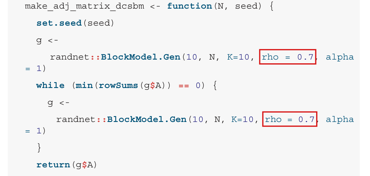
In the printed call to randnet::BlockModel.Gen, the argument rho = 0.7 is the probability that a unit receives the low degree weight 0.20.2, and every edge of the generated network lies within a community; the proportion of edges within a community is 1, not 0.7.

Section “Examples”, p. 214 (PDF p. 6), paragraph below Figure 16.2; code for make_adj_matrix_dcsbm, p. 215 (PDF p. 7)

See also under Formal statements (Lean): P044-T10

As printed

p. 214: “In particular, we generate a network according to a DCBM with N=1000N=1000 units, 10 communities (or clusters); where units are assigned to one of the 10 communities uniformly at random, and an expected proportion of edges that is within a community of 0.7.”

p. 215, in both calls to the generator (line break of the printed code joined):

randnet::BlockModel.Gen(10, N, K=10, rho = 0.7, alpha = 1)

The problem

The text reads the argument rho = 0.7 of the generator as the proportion of edges within communities. In randnet::BlockModel.Gen the argument has a different meaning. Between-community connection probabilities are controlled by beta, relative to within-community connection probabilities. The printed call does not pass beta, and its default is 00. The block probability matrix is then diagonal, and no edge joins two communities. Under the default simple = TRUE, the argument rho is the probability that a unit is given the degree weight 0.20.2 in place of 11, and alpha is not used. The second example network is therefore misdescribed, and it cannot be recovered from the sentence.

Evidence a check of the printed page

I checked the source code of the generator and a recalculation. In randnet 0.5, the arguments of BlockModel.Gen have the defaults beta=0, rho=0, simple=TRUE and alpha=5. The function sets the block matrix to diag(w) and fills its off-diagonal entries only if(beta > 0), and in the simple branch it sets node.degree[runif(n)<rho] <- 0.2. The manual describes beta as the “out-in ratio: the ratio of between-block edges over within-block edges”. The code of the generator is the same in versions 0.4, 0.5 and 0.7. The chapter does not say which version it used.

When the printed function is run with seed 42, the loop accepts the 193rd draw. The accepted network has all of its edges within communities and ten connected components. A share 0.7230.723 of its units have weight 0.20.2, its mean degree is 9.8589.858, its degree variance is 75.8775.87 and its skewness is 1.0751.075. It reproduces the six effect estimates and the six variance estimates that are printed for the DCBM on p. 218, to their printed precision.

What survives

The degree variance of 75 and the skewness of 1.07 quoted in the same paragraph approximate those of the network that the printed code generates. The printed DCBM estimates follow from that network. The definitions, the estimand and the design-based arguments do not depend on the proportion of edges within communities, and the small-world network is unaffected. If a network with 70% of its edges within communities was intended, the settings of the generator would have to be changed and the DCBM example recomputed.

Corrected

“In particular, we generate a network according to a DCBM with N=1000N=1000 units, 10 communities (or clusters); where units are assigned to one of the 10 communities uniformly at random, and all edges are within communities. Before graphs with isolated vertices are rejected, each unit is given the degree weight 0.2 with probability 0.7 and the weight 1 otherwise.”

Crop of six lines of text. Red boxes mark the words 'an expected proportion of edges that is within a community of 0.7', which run over two lines of the sentence that begins 'In particular, we generate a network according to a DCBM'.
Section “Examples”, p. 214 (PDF p. 6), paragraph below Figure 16.2. The marked words give 0.7 as the expected proportion of edges within a community.
Crop of the printed R function make_adj_matrix_dcsbm. Red boxes mark 'rho = 0.7' in each of the two calls randnet::BlockModel.Gen(10, N, K=10, rho = 0.7, alpha = 1). The second call is inside a while loop that repeats while some row sum of the adjacency matrix is zero.
Code on p. 215 (PDF p. 7), function make_adj_matrix_dcsbm. The marked argument rho = 0.7 appears in both calls to the generator; the argument beta is not passed.

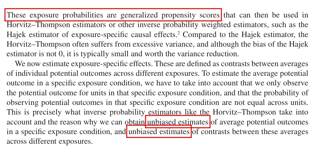
The Horvitz–Thompson estimators are unbiased with the true positive exposure probabilities of the design; make_exposure_prob returns smoothed frequencies, (c+1)/(R+1)(c+1)/(R+1), even when every assignment of the design is supplied, and the estimates computed from them are not exactly unbiased.

p. 216 (PDF p. 8), the two paragraphs after the make_exposure_prob calls; p. 212 (PDF p. 4), last paragraph. The routine is in the R package interference, R/make_exposure_prob.R, lines 83 and 88, and is not printed in the chapter.

See also under Formal statements (Lean): P044-T7, P044-T8

As printed

p. 216: “These exposure probabilities are generalized propensity scores that can then be used in Horvitz–Thompson estimators or other inverse probability weighted estimators, such as the Hajek estimator of exposure-specific causal effects.”

p. 216: “This is precisely what inverse probability estimators like the Horvitz–Thompson take into account and the reason why we can obtain unbiased estimates of average potential outcomes in a specific exposure condition, and unbiased estimates of contrasts between these averages across different exposures.”

p. 212: “The probabilities can be used to construct unbiased Horvitz-Thompson estimators of the τ(d,d′)\tau(d,d') effects or consistent and considerably more efficient Hajek or weighted least squares estimators.”

R/make_exposure_prob.R, lines 83 and 88 (same-exposure and cross-exposure matrices):

(I_exposure[[i]] %*% t(I_exposure[[i]]) + diag(N)) / (R + 1)

(I_exposure[[i]] %*% t(I_exposure[[j]])) / R

The problem

The statement is correct for the true exposure probabilities πi(d)=Pr⁡(Di=d)\pi_i(d)=\Pr(D_i=d), when they are positive. The routine that computes “these exposure probabilities” does not return them. Let ci(d)c_i(d) denote the number of the RR supplied assignments under which unit ii has exposure dd, and let cij(d,d′)c_{ij}(d,d') denote the number under which unit ii has exposure dd and unit jj has exposure d′d'. The routine returns (ci(d)+1)/(R+1)(c_i(d)+1)/(R+1) for the probability that unit ii has exposure dd, cij(d,d)/(R+1)c_{ij}(d,d)/(R+1) for the joint probability of two different units in the same exposure, and cij(d,d′)/Rc_{ij}(d,d')/R for two different exposures. It does so even when the RR assignments are all the assignments of the design, a case that p. 214 allows (“the set of all possible (or a large random sample of all possible) treatment assignments”). The four returned probabilities of a unit sum to (R+4)/(R+1)(R+4)/(R+1), which exceeds 1. Weighting by their inverses does not give an exactly unbiased estimator. The chapter does not mention the smoothing.

Evidence an exact counterexample

The evidence is an exact counterexample, which I also ran through the unchanged functions of the package. Let eight units form a cycle, and let the design be uniform on the eight rotations of the assignment (1,1,0,1,0,0,0,0)(1,1,0,1,0,0,0,0). Every assignment places two units in d11d_{11}, one in d10d_{10}, three in d01d_{01} and two in d00d_{00}, and every unit has the true exposure probabilities (1/4,1/8,3/8,1/4)(1/4,1/8,3/8,1/4). Supplied with all eight assignments, the routine returns (1/3,2/9,4/9,1/3)(1/3,2/9,4/9,1/3), which sum to 4/34/3. Let every unit have potential outcomes (2,3/2,5/4,1)(2,3/2,5/4,1) under (d11,d10,d01,d00)(d_{11},d_{10},d_{01},d_{00}). Then τ(d11,d00)=1\tau(d_{11},d_{00})=1, τ(d10,d00)=1/2\tau(d_{10},d_{00})=1/2 and τ(d01,d00)=1/4\tau(d_{01},d_{00})=1/4. With the returned probabilities, the Horvitz–Thompson contrasts equal 3/43/4, 3/323/32 and 39/12839/128 under every assignment, and these values are their expectations. With the true probabilities they equal 11, 1/21/2 and 1/41/4.

The general computation is short. Let qi(d)q_i(d) be positive weights used in place of πi(d)\pi_i(d). Since E[1{Di=d}]=πi(d)\mathbb{E}[\mathbf{1}\{D_i=d\}]=\pi_i(d), I have

E[1N∑i=1N1{Di=d} yi(d)qi(d)]=1N∑i=1Nyi(d) πi(d)qi(d).\mathbb{E}\Bigl[\frac{1}{N}\sum_{i=1}^{N}\frac{\mathbf{1}\{D_i=d\}\,y_i(d)}{q_i(d)}\Bigr]=\frac{1}{N}\sum_{i=1}^{N}y_i(d)\,\frac{\pi_i(d)}{q_i(d)}.

For a design of RR equally likely assignments, all supplied, πi(d)=ci(d)/R\pi_i(d)=c_i(d)/R and qi(d)=(ci(d)+1)/(R+1)q_i(d)=(c_i(d)+1)/(R+1). The ratio πi(d)/qi(d)\pi_i(d)/q_i(d) then equals ci(d)(R+1)/(R(ci(d)+1))c_i(d)(R+1)/\bigl(R(c_i(d)+1)\bigr), which differs from 1 whenever 0<ci(d)<R0<c_i(d)<R.

What survives

The exposure mapping and the estimands are unaffected, and the Horvitz–Thompson estimator remains unbiased when the exposure probabilities are the true ones and are positive. The chapter already says that the Hajek estimator is biased. The estimator computed from the package’s probabilities has no guarantee of exact unbiasedness, even when all assignments are enumerated. The counterexample does not measure the bias at the chapter’s R=10,000R=10{,}000. The recalculation made for P044-N009 measures it on the degree-corrected block model generated by the printed code. There, conditional on the chapter’s simulated probabilities and with an independent assignment, the expectation of the Horvitz–Thompson estimator exceeds the true effect by 0.5%, 1.5% and 0.9% for (d11,d00)(d_{11},d_{00}), (d10,d00)(d_{10},d_{00}) and (d01,d00)(d_{01},d_{00}). No entry of Table 16.1 and no comparison of Figure 16.3 is shown to change.

Corrected

Let πi(d)=Pr⁡(Di=d)\pi_i(d)=\Pr(D_i=d) be the true exposure probabilities of the design and Yi=yi(Di)Y_i=y_i(D_i) the observed outcome. If πi(d)>0\pi_i(d)>0 and πi(d′)>0\pi_i(d')>0 for every unit ii, then the Horvitz–Thompson estimator

τ^HT(d,d′)=1N∑i=1N(1{Di=d} Yiπi(d)−1{Di=d′} Yiπi(d′))\widehat\tau_{HT}(d,d')=\frac{1}{N}\sum_{i=1}^{N}\Bigl(\frac{\mathbf{1}\{D_i=d\}\,Y_i}{\pi_i(d)}-\frac{\mathbf{1}\{D_i=d'\}\,Y_i}{\pi_i(d')}\Bigr)

is unbiased for τ(d,d′)\tau(d,d'). The exposure probabilities computed on p. 216 are frequencies over R=10,000R=10{,}000 simulated assignments, smoothed as (c+1)/(R+1)(c+1)/(R+1), and the estimates computed from them have no guarantee of exact unbiasedness. When all RR equally likely assignments of a design are enumerated, the exact probabilities are ci(d)/R\colorbox{#ffe58a}{$c_i(d)/R$} and cij(d,d′)/R\colorbox{#ffe58a}{$c_{ij}(d,d')/R$}, and line 83 of the routine should then read

(I_exposure[[i]] %*% t(I_exposure[[i]])) / R

Crop of two paragraphs of running text. A red box marks the opening words 'These exposure probabilities are generalized propensity scores'. In the second paragraph, red boxes mark the words 'unbiased estimates' twice, in the sentence 'the reason why we can obtain unbiased estimates of average potential outcomes in a specific exposure condition, and unbiased estimates of contrasts between these averages across different exposures'.
p. 216 (PDF p. 8), the two paragraphs after the make_exposure_prob calls. The first marked phrase refers to the output of the routine; the other two say that the estimates computed from it are unbiased.

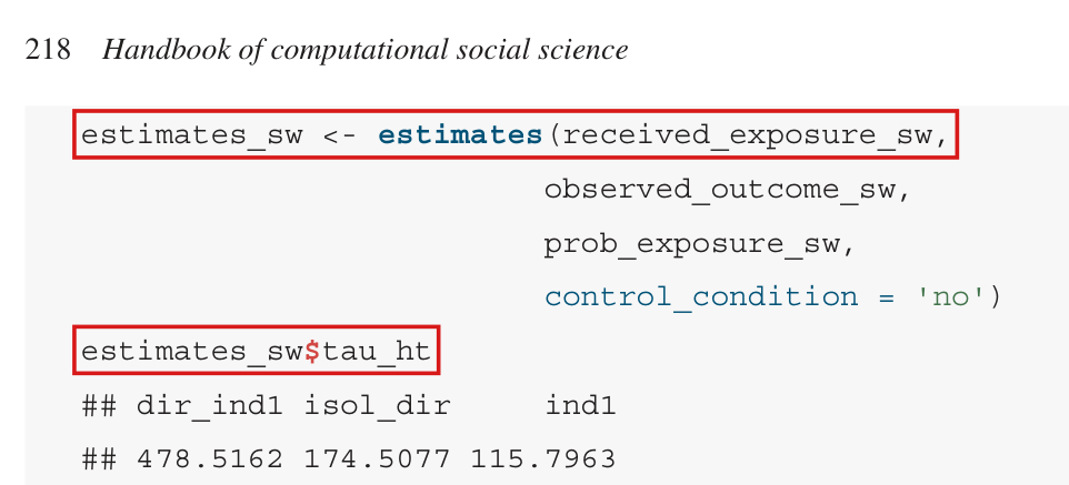
When no unit receives an exposure, the Horvitz–Thompson total for that exposure is zero and the contrast is defined; the package returns a missing value instead.

p. 218 (PDF p. 10), the calls to estimates() and the output tau_ht. The line at issue is in the R package interference, R/estimates.R, line 219 (also line 624, and R/estimates_batch.R, line 222), and is not printed in the chapter.

As printed

p. 218, joined on two lines:

estimates_sw <- estimates(received_exposure_sw, observed_outcome_sw,

prob_exposure_sw, control_condition = 'no')

estimates_sw$tau_ht

R/estimates.R, lines 216–219 (the first three joined on one line):

yT_ht <- rowSums(obs_outcome_by_exposure / obs_prob_exposure_individual_kk, na.rm = T)

yT_ht[rowSums(!is.na(obs_outcome_by_exposure)) == 0] <- NA

The problem

The package documents yT_ht as the Horvitz–Thompson estimator of the total of the potential outcomes under an exposure, T^d=∑i1{Di=d} Yi/πi(d)\widehat T_d=\sum_i\mathbf{1}\{D_i=d\}\,Y_i/\pi_i(d). When no unit receives dd, every term of the sum is zero and T^d=0\widehat T_d=0. Line 219 replaces this zero by NA. The contrast tau_ht is then missing, although the estimator that the chapter calls unbiased (pp. 212 and 216) equals a finite number. An average over the assignments for which the function returns a value conditions on a random event and can have a different expectation. A missing value is appropriate for the Hajek mean, which is 0/00/0 for an empty exposure.

Evidence an exact counterexample

The evidence is an exact counterexample, which I also ran on the unchanged function. Let six units form a cycle, and let two of them be treated, uniformly over the 15 assignments. Every unit has exposure probabilities (2/15,1/5,7/15,1/5)(2/15,1/5,7/15,1/5) for (d11,d10,d01,d00)(d_{11},d_{10},d_{01},d_{00}). Let every unit have potential outcomes (2,3/2,5/4,1)(2,3/2,5/4,1), so that τ(d11,d00)=1\tau(d_{11},d_{00})=1. Under the assignment (1,0,1,0,0,0)(1,0,1,0,0,0) no unit receives d11d_{11} and one unit receives d00d_{00}. The totals are T^d11=0\widehat T_{d_{11}}=0 and T^d00=5\widehat T_{d_{00}}=5, and the Horvitz–Thompson contrast is (0−5)/6=−5/6(0-5)/6=-5/6. The function returns NA. Over the 15 assignments, the contrast equals 10/310/3 six times (the two treated units are adjacent), −5/6-5/6 six times and 00 three times, and its mean is 1. The function returns a value only in the first six cases, and the mean of the returned values is 10/310/3. With the overwrite removed, the function returns the exact totals and contrasts under all 15 assignments.

The general statement takes one line. Since 1{Di=d} Yi=1{Di=d} yi(d)\mathbf{1}\{D_i=d\}\,Y_i=\mathbf{1}\{D_i=d\}\,y_i(d) and πi(d)>0\pi_i(d)>0, I have E[1{Di=d} Yi/πi(d)]=yi(d)\mathbb{E}\bigl[\mathbf{1}\{D_i=d\}\,Y_i/\pi_i(d)\bigr]=y_i(d) for each unit, whether or not the exposure occurs under a given assignment. Summing over ii gives E[T^d]=∑iyi(d)\mathbb{E}[\widehat T_d]=\sum_i y_i(d), which implies that E[(T^d−T^d′)/N]=τ(d,d′)\mathbb{E}\bigl[(\widehat T_d-\widehat T_{d'})/N\bigr]=\tau(d,d').

What survives

The Horvitz–Thompson estimator remains unbiased when the exposure probabilities are the true ones and are positive. The estimands are unaffected, and so are the point estimates under any assignment in which every exposure occurs. Table 16.1 prints finite estimates, and no entry of it and no result of Figure 16.3 is shown to change. I did not estimate how often an exposure is empty on the chapter’s networks of 1000 units. The correction concerns the point totals only and implies nothing about the variance estimators.

Corrected

Let πi(d)>0\pi_i(d)>0 for every unit ii. The Horvitz–Thompson total under exposure dd is T^d=∑i=1N1{Di=d} Yi/πi(d)\widehat T_d=\sum_{i=1}^{N}\mathbf{1}\{D_i=d\}\,Y_i/\pi_i(d), which equals 0 when no unit receives dd. If also πi(d′)>0\pi_i(d')>0 for every ii, then τ^HT(d,d′)=(T^d−T^d′)/N\widehat\tau_{HT}(d,d')=(\widehat T_d-\widehat T_{d'})/N is defined under every assignment and is unbiased for τ(d,d′)\tau(d,d'). In the package, R/estimates.R, lines 216–219, with line 219 deleted:

yT_ht <- rowSums(obs_outcome_by_exposure / obs_prob_exposure_individual_kk, na.rm = T)

The same line should be deleted at R/estimates.R, line 624, and at R/estimates_batch.R, line 222. The change applies when all outcomes are observed; outcomes that are themselves missing need separate handling. The Hajek mean of an empty exposure remains missing, and the variance code is not repaired by this change.

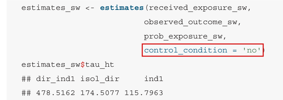
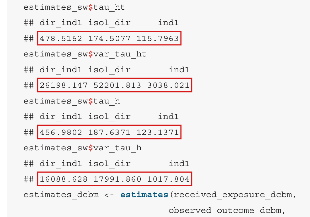
Code listing under the page header '218 Handbook of computational social science'. Red boxes mark the first line of the call, estimates_sw <- estimates(received_exposure_sw, and the line estimates_sw$tau_ht. The call continues with observed_outcome_sw, prob_exposure_sw and control_condition = 'no'. The output below shows dir_ind1 478.5162, isol_dir 174.5077 and ind1 115.7963.
p. 218 (PDF p. 10): the call to estimates() and the Horvitz–Thompson contrasts that it returns. The package line that sets the total of an empty exposure to NA is not printed in the chapter; the marks identify the function call and its point-contrast output.

The function estimates() takes its point contrasts against the exposure named 'no' whatever control_condition is supplied; they should be taken against the supplied control condition, and the chapter’s calls, which supply 'no', are unaffected.

p. 218 (PDF p. 10), the two calls estimates(..., control_condition = 'no'). The lines at issue are in the R package interference, R/estimates.R, lines 314, 318 and 333–336, and are not printed in the chapter.

As printed

p. 218, joined on two lines:

estimates_sw <- estimates(received_exposure_sw, observed_outcome_sw,

prob_exposure_sw, control_condition = 'no')

R/estimates.R, lines 314 and 318:

tau_ht <- (1 / N) * (yT_ht - yT_ht['no'])[names(yT_ht) != 'no']

tau_h <- (mu_h - mu_h['no'])[names(mu_h) != 'no']

The problem

The argument control_condition names the exposure against which the other exposures are contrasted, and the variance estimates that the function returns by default, var_tau_ht and var_tau_h, use it. The point contrasts tau_ht, tau_h and tau_dsm do not: they subtract, and exclude, the exposure literally named 'no'. If the no-exposure condition has another name, which an exposure mapping defined by the user (pp. 215–216) may give it, every point contrast is NA. If another exposure is requested as the control condition, the point contrasts are still taken against 'no', while the variance estimates are those of the contrasts against the requested control condition. The estimates and their variances then refer to different contrasts.

Evidence an exact counterexample

The evidence is an exact counterexample, which I also ran on the unchanged function. Let eight units form a cycle, let three of them be treated, uniformly over the 56 assignments, and let yi(d)=iy_i(d)=i for every exposure dd. Every unit has exposure probabilities (11/56,5/28,25/56,5/28)(11/56,5/28,25/56,5/28) for (d11,d10,d01,d00)(d_{11},d_{10},d_{01},d_{00}). Under the assignment (1,1,0,0,1,0,0,0)(1,1,0,0,1,0,0,0) every exposure occurs, and the Horvitz–Thompson totals are (168/11, 28, 1176/25, 196/5)(168/11,\,28,\,1176/25,\,196/5). With control_condition = 'ind1', the contrast of d11d_{11} against d01d_{01} is (168/11−1176/25)/8=−1092/275(168/11-1176/25)/8=-1092/275. The function returns (168/11−196/5)/8=−329/110(168/11-196/5)/8=-329/110, the contrast against d00d_{00}, in a vector with the names dir_ind1, isol_dir, ind1. Its variance estimates carry the names dir_ind1, isol_dir, no and are those of the contrasts against d01d_{01}. When I rename 'no' as 'baseline' throughout and supply control_condition = 'baseline', each of the three point vectors consists of four NA values. The three entries of each default variance vector are finite and unchanged. With the corrected lines for tau_ht, tau_h and tau_dsm, the function returns the requested contrasts in both cases, and its output for control_condition = 'no' is unchanged.

What survives

The definition of the contrasts τ(d,d′)\tau(d,d'), the totals and means for each exposure, and calls that supply control_condition = 'no' are unaffected by this defect. The two calls on p. 218 supply 'no', Table 16.1 takes d00d_{00} as the reference, and nothing reported in the chapter changes. The correction is to the package.

Corrected

Let control_condition name a single existing exposure. In R/estimates.R, lines 314, 318 and 333–336, each statement on two lines:

tau_ht <- (1 / N) * (yT_ht - yT_ht[control_condition])[

names(yT_ht) != control_condition]

tau_h <- (mu_h - mu_h[control_condition])[

names(mu_h) != control_condition]

means_dsm <- rowMeans(obs_outcome_by_exposure, na.rm = TRUE)

tau_dsm <- (means_dsm - means_dsm[control_condition])[

names(means_dsm) != control_condition]

In R/estimates_batch.R, lines 248 and 252, the same replacement applies to the Horvitz–Thompson and Hajek contrasts. Lines 262–263 of R/estimates.R belong to the optional constant-effect variance estimator and would read as follows; I did not run that branch.

diffs <- const_eff$means - const_eff$means[[control_condition]]

diffs <- diffs[, names(diffs) != control_condition, with = FALSE]

Code listing. The call reads estimates_sw <- estimates(received_exposure_sw, observed_outcome_sw, prob_exposure_sw, control_condition = 'no'), and a red box marks the argument control_condition = 'no'. Below it are the line estimates_sw$tau_ht and the output dir_ind1 478.5162, isol_dir 174.5077, ind1 115.7963.
p. 218 (PDF p. 10): the call to estimates(). The marked argument names the control condition. The chapter supplies 'no', the one value for which the point contrasts are computed as requested.

In the statements of no interference and of interference, the second argument of the potential outcome is the vector of the other units' assignments, and in the exposure-mapping display the count of treated peers is the scalar θiz\theta_i\mathbf{z}.

Section “Network experimental setting”, p. 211 (PDF p. 3), second paragraph, statements of no interference and of interference; Section “Exposure mappings and causal effects”, p. 211 (PDF p. 3), display defining f(z,θi)f(\mathbf{z},\theta_i); definition of z\mathbf{z}, p. 210 (PDF p. 2)

See also under Formal statements (Lean): P044-T9

As printed

p. 210: “The N×1N\times 1 vector of treatments for all units is given by z=(z1,…,zN)′\mathbf{z}=(z_1,\ldots,z_N)'.”

p. 211: “Then we can also denote unit ii's potential outcome as yi(zi;z−i)y_i(z_i;\mathbf{z}_{-i}). … Traditional analyses of experiments assume no interference, which would imply that unit ii's outcome depends only on the element ziz_i; that is, for any z\mathbf{z} and z′\mathbf{z}', yi(zi;z)=yi(zi;z′)y_i(z_i;\colorbox{#ffe58a}{$\mathbf{z}$})=y_i(z_i;\colorbox{#ffe58a}{$\mathbf{z}'$}). Interference means for some unit i∈Ui\in U we have yi(zi;z)≠yi(zi;z′)y_i(z_i;\colorbox{#ffe58a}{$\mathbf{z}$})\neq y_i(z_i;\colorbox{#ffe58a}{$\mathbf{z}'$}).”

p. 211: “This would imply an exposure mapping that takes as inputs the assignment profile z\mathbf{z} and unit ii's row in the adjacency matrix, θi\theta_i, as follows:” The display that follows is

f(z,θi)={d11(Direct+IndirectExposure):ziI(z′θi>0)=1,d10(IsolatedDirectExposure):ziI(z′θi=0)=1,d01(IndirectExposure):(1−zi)I(z′θi>0)=1,d00(NoExposure):(1−zi)I(z′θi=0)=1f(\mathbf{z},\theta_i)=\begin{cases} d_{11}(\text{Direct}+\text{IndirectExposure}): & z_i\mathbf{I}(\colorbox{#ffe58a}{$\displaystyle \mathbf{z}'\theta_i$}>0)=1,\\ d_{10}(\text{IsolatedDirectExposure}): & z_i\mathbf{I}(\colorbox{#ffe58a}{$\displaystyle \mathbf{z}'\theta_i$}=0)=1,\\ d_{01}(\text{IndirectExposure}): & (1-z_i)\mathbf{I}(\colorbox{#ffe58a}{$\displaystyle \mathbf{z}'\theta_i$}>0)=1,\\ d_{00}(\text{NoExposure}): & (1-z_i)\mathbf{I}(\colorbox{#ffe58a}{$\displaystyle \mathbf{z}'\theta_i$}=0)=1 \end{cases}
The problem

Two pieces of notation on p. 211 do not match the definitions given just before them. First, the potential outcome with two arguments is defined as yi(zi;z−i)y_i(z_i;\mathbf{z}_{-i}), with the (N−1)(N-1)-vector of the other units' assignments in the second place. The four expressions that follow carry the full vectors z\mathbf{z} and z′\mathbf{z}' there, without the subscript −i-i, so that the assignment of unit ii itself enters twice. Second, z\mathbf{z} is an N×1N\times 1 column and θi\theta_i is unit ii's row of the adjacency matrix. Then z′\mathbf{z}' and θi\theta_i are both 1×N1\times N, and the product z′θi\mathbf{z}'\theta_i is not defined for N>1N>1. The intended meaning is clear in both places, and it is correct. Under no interference, the assignments of the other units do not change unit ii's outcome when its own assignment is held fixed. The indicator in the display tests whether at least one of unit ii's peers is treated.

Evidence a derivation

I checked the pages and the following derivation. For a∈{0,1}a\in\{0,1\} and u∈{0,1}N−1\mathbf{u}\in\{0,1\}^{N-1}, let yi(a;u)y_i(a;\mathbf{u}) denote yiy_i evaluated at the profile obtained by inserting aa in position ii of u\mathbf{u}. No interference is the statement that yi(a;u)=yi(a;v)y_i(a;\mathbf{u})=y_i(a;\mathbf{v}) for all ii, aa, u\mathbf{u} and v\mathbf{v}. Interference is its negation, in which the two vectors of assignments are quantified existentially. For the display, the product of the 1×N1\times N row θi\theta_i and the N×1N\times 1 column z\mathbf{z} is the scalar

θiz=∑j=1Nθijzj.\theta_i\mathbf{z}=\sum_{j=1}^N\theta_{ij}z_j .

By the definition of θ\theta on p. 210, its entries are 00 or 11 and its diagonal is zero. The sum counts the treated units among those whose treatment may affect unit ii, and it is positive exactly when at least one of them is treated.

What survives

Nothing else in the chapter depends on these misprints. The definition of interference, the four exposure conditions, the estimand and all later analysis are unchanged.

Corrected

Let yi(a;u)y_i(a;\mathbf{u}) denote unit ii's potential outcome when its own assignment is a∈{0,1}a\in\{0,1\} and the assignments of the other N−1N-1 units are u∈{0,1}N−1\mathbf{u}\in\{0,1\}^{N-1}.

“… that is, for every unit ii, every a∈{0,1}a\in\{0,1\} and all u,v∈{0,1}N−1\mathbf{u},\mathbf{v}\in\{0,1\}^{N-1}, yi(a;u)=yi(a;v)y_i(a;\colorbox{#ffe58a}{$\mathbf{u}$})=y_i(a;\colorbox{#ffe58a}{$\mathbf{v}$}). Interference means that there exist a unit i∈Ui\in U, a value a∈{0,1}a\in\{0,1\} and vectors u,v∈{0,1}N−1\mathbf{u},\mathbf{v}\in\{0,1\}^{N-1} such that yi(a;u)≠yi(a;v)y_i(a;\colorbox{#ffe58a}{$\mathbf{u}$})\neq y_i(a;\colorbox{#ffe58a}{$\mathbf{v}$}).”

With θi\theta_i the iith row of the adjacency matrix and z\mathbf{z} the N×1N\times 1 column of assignments,

f(z,θi)={d11(Direct+IndirectExposure):ziI(θiz>0)=1,d10(IsolatedDirectExposure):ziI(θiz=0)=1,d01(IndirectExposure):(1−zi)I(θiz>0)=1,d00(NoExposure):(1−zi)I(θiz=0)=1,f(\mathbf{z},\theta_i)=\begin{cases} d_{11}(\text{Direct}+\text{IndirectExposure}): & z_i\mathbf{I}(\colorbox{#ffe58a}{$\displaystyle \theta_i\mathbf{z}$}>0)=1,\\ d_{10}(\text{IsolatedDirectExposure}): & z_i\mathbf{I}(\colorbox{#ffe58a}{$\displaystyle \theta_i\mathbf{z}$}=0)=1,\\ d_{01}(\text{IndirectExposure}): & (1-z_i)\mathbf{I}(\colorbox{#ffe58a}{$\displaystyle \theta_i\mathbf{z}$}>0)=1,\\ d_{00}(\text{NoExposure}): & (1-z_i)\mathbf{I}(\colorbox{#ffe58a}{$\displaystyle \theta_i\mathbf{z}$}=0)=1, \end{cases}

where θiz=∑j=1Nθijzj\theta_i\mathbf{z}=\sum_{j=1}^N\theta_{ij}z_j.

Crop of eight lines of text. The first line ends the definition of the potential outcome y i of z i and z minus i. Four red boxes mark the bold z and the bold z prime that stand as second arguments in 'y i of z i; z equals y i of z i; z prime' and in 'y i of z i; z is not equal to y i of z i; z prime'.
Section “Network experimental setting”, p. 211 (PDF p. 3), second paragraph. The four marked second arguments are the full vectors z\mathbf{z} and z′\mathbf{z}'; the definition in the first line of the crop has z−i\mathbf{z}_{-i} in that place.
Crop of three lines of text and a display of four lines. A red box marks the word 'row' in 'unit i's row in the adjacency matrix, theta i'. Four more red boxes mark the product z prime theta i inside the indicator in each of the four lines of the display.
Section “Exposure mappings and causal effects”, p. 211 (PDF p. 3), the display defining f(z,θi)f(\mathbf{z},\theta_i). The marked word says that θi\theta_i is a row, and each of the four marked products multiplies the row z′\mathbf{z}' by it.

In Figure 16.1, unit 2 is tied to units 1, 3, 4 and 10; the other peers of unit 3 to which it is tied are units 4 and 1, and unit 5 is not among them.

Section “Design-based inference”, p. 213 (PDF p. 5), first paragraph; Figure 16.1, p. 210 (PDF p. 2)

As printed

“In the network in Figure 16.1, we can see that units 1 and 2 are both connected to unit 3, creating a dependency on whether these two units will receive indirect exposure. However, unit 2 is also tied to other peers of unit 3: units 5, 4, and 1.”

The problem

The list includes unit 5, and Figure 16.1 shows no edge between units 2 and 5. The edge from unit 2 to unit 4 is drawn behind the disk of vertex 5, and this makes it look like an edge to unit 5. The point of the passage is that units with shared peers have dependent exposures. That point is correct, and units 4 and 1 illustrate it.

Evidence a check of the printed page

I checked the figure. In the image embedded in the PDF, a line was fitted to the visible part of the stroke that leaves vertex 2 toward the lower right. The line passes within 0.30.3 pixels of the centres of vertices 2 and 4, and it misses the centre of vertex 5 by about 2323 pixels. The stroke continues below vertex 5 to vertex 4.

What survives

No estimator, result or calculation depends on the list. The statement about dependence through shared peers stands.

Corrected

“However, unit 2 is also tied to other peers of unit 3: units 4 and 1.”

Crop of five lines of text. A red box marks '5,' in the sentence 'However, unit 2 is also tied to other peers of unit 3: units 5, 4, and 1.'
Section “Design-based inference”, p. 213 (PDF p. 5), first paragraph. The marked unit 5 is not tied to unit 2 in Figure 16.1.
Drawing of a network with ten numbered vertices. A red box marks vertex 5, which lies between vertex 2, above it and to its left, and vertex 4, below it. A grey stroke leaves vertex 2 toward the lower right, disappears behind the disk of vertex 5 and reappears below it, beside a second stroke, to reach vertex 4. Vertex 2 has other strokes to vertices 1, 3 and 10.
Figure 16.1, p. 210 (PDF p. 2). The stroke that leaves vertex 2 toward the lower right passes behind the marked vertex 5 and ends at vertex 4; no edge joins vertices 2 and 5.

Under R 4.4.2 and igraph 2.2.2, the printed generator and seeds do not reproduce the printed results for the small-world network, and the chapter does not state the software versions needed to reproduce them.

Section “Examples”, p. 214 (PDF p. 6), paragraph below Figure 16.2; code for make_adj_matrix_small_world, p. 215 (PDF p. 7); output for estimates_sw, p. 218 (PDF p. 10); Table 16.1, Small-World columns, p. 219 (PDF p. 11)

As printed

p. 214: “… the vertex degree distribution in this DCBM is also substantially more skewed (with a skewness of 1.07) than the vertex degree distribution in the small-world network (with a skewness of 0.12).”

p. 215 (line breaks of the printed code joined):

set.seed(seed)

g <- igraph::sample_smallworld(dim=1, size=N, nei=5, p=0.1)

adj_matrix_sw <- make_adj_matrix_small_world(N, seed = 42)

p. 218, output in the columns dir_ind1, isol_dir, ind1:

estimates_sw$tau_ht: 478.5162, 174.5077, 115.7963

estimates_sw$var_tau_ht: 26198.147, 52201.813, 3038.021

estimates_sw$tau_h: 456.9802, 187.6371, 123.1371

estimates_sw$var_tau_h: 16088.628, 17991.860, 1017.804

The problem

The small-world half of the worked example cannot be reproduced from the printed code. Under R 4.4.2 and igraph 2.2.2, the printed generator with seed 42 generates a network whose degree skewness is 0.07, where the chapter prints 0.12. Its mean degree is 10 and its degree variance rounds to 2, as printed. When that network is carried through the rest of the printed code with the printed seeds, every estimate and every variance estimate differs from the output on p. 218, and from the Small-World columns of Table 16.1, which agree with that output. A seed fixes the state of a random number generator, and it does not fix the implementation of sample_smallworld. The chapter states no version of R or of igraph, and no archive of the network that it used has been located. This is a gap in reproducibility. It does not show that any printed number is wrong for the network that the chapter used.

Evidence a recalculation from the source

I checked a recalculation from the printed code and the source of the interference package (version 0.1.0). The regenerated network has 5000 edges and degrees from 5 to 15. In exact arithmetic, its degree variance is 233/125233/125 and its third central moment is 9/509/50, which implies that the skewness lies between 0.070720.07072 and 0.070740.07074. The adjusted skewness also rounds to 0.07. The two sampling rules of R, the R 4.4.2 default (“Rejection”) and the older one (“Rounding”), give the same network and different assignments, and neither reproduces the printed output.

Small-world estimates: the output printed on p. 218 and the values obtained from the printed code and seeds under R 4.4.2 and igraph 2.2.2, for each sampling rule.
EstimatePrintedRegenerated, RejectionRegenerated, Rounding
Horvitz–Thompson, (d11,d00)(d_{11},d_{00})478.5162388.58314.98
Horvitz–Thompson, (d10,d00)(d_{10},d_{00})174.5077448.62170.37
Horvitz–Thompson, (d01,d00)(d_{01},d_{00})115.7963152.29−9.21-9.21
Hajek, (d11,d00)(d_{11},d_{00})456.9802529.16389.37
Hajek, (d10,d00)(d_{10},d_{00})187.6371244.61225.87
Hajek, (d01,d00)(d_{01},d_{00})123.1371142.75117.27

The variance estimates differ in the same way. Table 16.1 agrees with the printed output: its 18 Small-World entries (estimates, standard errors and tt-statistics) match the printed output after truncation to two decimal places.

What survives

The exposure mapping, the estimands and the design-based arguments are untouched, and so is the role of the example as an illustration. The regenerated network still has mean degree 10, a degree variance near 2 and a tight degree distribution. The DCBM results and Figure 16.3 are not shown wrong by this point. What cannot be done from the printed code alone is to reproduce the degree summary of the small-world network, the output on p. 218 and the Small-World columns of Table 16.1.

Corrected

No printed value is replaced. The correction is an addition: the chapter should state the versions of R, igraph and the interference package, the kind of random number generator and the seeds with which the results were obtained, and the small-world network, the realized assignment and the 10,000 sampled assignments should be archived.

If instead a new network is generated under R 4.4.2 and igraph 2.2.2, the degree summary on p. 214, Figure 16.2, the output on p. 218 and the Small-World columns of Table 16.1 must all be replaced together. Changing 0.12 to 0.07 alone would not make the printed output reproducible.

Crop of five lines of text. A red box marks '0.12' in the words 'than the vertex degree distribution in the small-world network (with a skewness of 0.12)'.
Section “Examples”, p. 214 (PDF p. 6). The marked skewness of the small-world network is 0.12; the network regenerated from the printed code under R 4.4.2 and igraph 2.2.2 has 0.07.
Crop of the printed R function make_adj_matrix_small_world and the line that calls it. Red boxes mark the call igraph::sample_smallworld(dim=1, size=N, nei=5, p=0.1), which runs over two lines, and the argument 'seed = 42' in the line adj_matrix_sw <- make_adj_matrix_small_world(N, seed = 42).
Code on p. 215 (PDF p. 7), function make_adj_matrix_small_world. The marked call and the marked seed are all that the chapter gives to determine the small-world network.
Crop of printed R output. Red boxes mark four rows of numbers: 478.5162 174.5077 115.7963 under the heading tau_ht; 26198.147 52201.813 3038.021 under var_tau_ht; 456.9802 187.6371 123.1371 under tau_h; and 16088.628 17991.860 1017.804 under var_tau_h. The columns are headed dir_ind1, isol_dir and ind1.
Output on p. 218 (PDF p. 10) for estimates_sw. The four marked rows are the printed small-world estimates and variance estimates; none of them is obtained when the printed code is run under R 4.4.2 and igraph 2.2.2.

The upper panel of Figure 16.3 plots the bias as a proportion of the true effect, not in percent as its label “bias (%)” says: the Hajek biases plotted for the degree-corrected block model, near 0.042, 0.106 and −0.148-0.148, are about 4%, 11% and −15%-15\% of the effect, not 0.04%, 0.11% and −0.15%-0.15\%.

Figure 16.3, p. 220 (PDF p. 12), upper panel, strip label “bias (%)”

As printed

Figure 16.3, upper panel: strip label “bias (%)”, with ticks labelled 0.10, 0.05, 0.00, −0.05-0.05, −0.10-0.10, −0.15-0.15. The points for the Hajek estimator on the degree-corrected block model (red circles) lie at about 0.0420.042 for dir_ind, 0.1060.106 for ind and −0.148-0.148 for isol_dir.

The problem

The strip label of the upper panel reads “bias (%)”, and the labelled ticks run from −0.15-0.15 to 0.100.10. Read as labelled, the largest absolute bias in the panel is about 0.15% of the effect. The plotted values are proportions. They agree, within Monte Carlo variability, with a recalculation of the mean estimate minus the true effect, divided by the true effect, with no factor of 100. This implies that the label understates every bias in the panel by a factor of 100. On the degree-corrected block model the plotted Hajek biases are about +4%+4\%, +11%+11\% and −15%-15\% of the effect for the three estimands, and not a few hundredths of one percent. The panel is the only evidence in the chapter on the size of this bias, and nothing on the page reveals the scale, since the chapter gives no formula for the plotted quantity (see P044-N010).

I infer the scale from a recalculation. The original plotting code and assignments were not found, so I do not recover the exact original biases.

Evidence a check of the printed page

The evidence is a recalculation. Running the printed code and seed for the degree-corrected block model (p. 215) with the generator of randnet 0.5, I obtain a network. With the potential outcomes, the exposure probabilities and the assignment generated as in the printed code, this network reproduces the six estimates and the six variance estimates that are printed for this model on p. 218, to within 5×10−55\times 10^{-5} and 4×10⁻³⁴\times 10^{-3}. This agreement ties the recalculation to the chapter’s printed example. On this network the true effects are τ(d11,d00)=623.80\tau(d_{11},d_{00})=623.80, τ(d01,d00)=155.95\tau(d_{01},d_{00})=155.95 and τ(d10,d00)=311.90\tau(d_{10},d_{00})=311.90.

I then kept the exposure probabilities fixed, drew R=100,000R=100{,}000 fresh assignments by complete randomization, and computed for each estimand the relative bias defined in the corrected passage below. For the Hajek estimator, I find the following values.

Hajek estimator on the degree-corrected block model: the value plotted in Figure 16.3, and the relative bias recalculated from 100,000 assignments, with its Monte Carlo standard error in parentheses.
EstimandTrue effectPlotted valueRecalculated relative biasIn percent
dir_ind, τ(d11,d00)\tau(d_{11},d_{00})623.800.0420.0420.04140.0414 (0.0015)(0.0015)4.14%
ind, τ(d01,d00)\tau(d_{01},d_{00})155.950.1060.1060.12490.1249 (0.0034)(0.0034)12.49%
isol_dir, τ(d10,d00)\tau(d_{10},d_{00})311.90−0.148-0.148−0.1367-0.1367 (0.0056)(0.0056)−13.67-13.67%

For 5000 assignments, the estimated Monte Carlo standard errors are larger than those of the table by the factor 20\sqrt{20}, namely 0.0068, 0.0152 and 0.0250. Read as proportions, the plotted values lie 0.2, 1.3 and 0.4 of these standard errors from the recalculated ones. Read as percentages, they lie 6.0, 8.2 and 5.4 standard errors away.

What survives

The lower panel is unaffected. The RMSE is in outcome units, and the Hajek estimator has the lower RMSE in all six cells. In the recalculation on the degree-corrected block model, I find an RMSE of 303, 168 and 554 for the Hajek estimator, against 396, 269 and 771 for the Horvitz–Thompson estimator, in the order of the figure. The estimands, the estimators and Table 16.1 do not depend on the label. The statements that the bias of the Hajek estimator is “typically small and worth the variance reduction” (p. 216), and that the variance reduction “overwhelms the increase in bias” (p. 219), are qualitative and stand at either scale. At the corrected scale, the three plotted absolute Hajek biases are about 4% to 15% of the effect.

I checked the scale only on the three Hajek points for the degree-corrected block model, and I did not recalculate the small-world example. The Horvitz–Thompson points share the axis and are on the same scale. I do not read them as Monte Carlo error alone. With exposure probabilities estimated from 10,000 assignments, the expected relative bias of the Horvitz–Thompson estimator on the regenerated network, computed exactly, is 0.005, 0.009 and 0.015 for the three estimands in the order of the figure.

Corrected

Figure 16.3, upper panel: strip label “relative bias (proportion)”, with the ticks 0.10, 0.05, 0.00, −0.05-0.05, −0.10-0.10, −0.15-0.15 unchanged. Here, for each network, each estimator τ^\widehat\tau and each estimand τ(d,d′)\tau(d,d'), I estimate relative bias by

estimated relative bias=τ‾R(d,d′)−τ(d,d′)τ(d,d′),τ‾R(d,d′)=1R∑r=1Rτ^r(d,d′),\colorbox{#ffe58a}{$\displaystyle \text{estimated}$}\ \text{relative bias}=\frac{\overline{\tau}_R(d,d')-\tau(d,d')}{\tau(d,d')},\qquad \overline{\tau}_R(d,d')=\frac{1}{R}\sum_{r=1}^{R}\widehat\tau_r(d,d'),

where τ^r(d,d′)\widehat\tau_r(d,d') is the estimate under the rrth of the R=5000R=5000 reassignments of treatment, and τ(d,d′)\tau(d,d') is the true average effect computed from the simulated potential outcomes.

Alternatively, the label “bias (%)” is kept and the plotted values and ticks are multiplied by 100, so that the ticks read 10\colorbox{#ffe58a}{$10$}, 5\colorbox{#ffe58a}{$5$}, 00, −5\colorbox{#ffe58a}{$-5$}, −10\colorbox{#ffe58a}{$-10$}, −15\colorbox{#ffe58a}{$-15$}.

Crop of page 220 from the running head, which reads 220 Handbook of computational social science, to the caption of Figure 16.3, which reads Estimator performance across networks. Two stacked panels share a horizontal axis named estimand, with categories dir\_ind, ind and isol\_dir, and a vertical axis named value. A red box marks the strip label of the upper panel, which reads bias (\%). The ticks of that panel are 0.10, 0.05, 0.00, -0.05, -0.10 and -0.15. Red points are the model dcBM and turquoise points the model small world; circles are the estimator Hajek and triangles the estimator HT. In the upper panel the red circles lie near 0.04, 0.11 and -0.15, the red triangles near -0.01, -0.02 and -0.03, and the turquoise points near zero. The lower panel has the strip label rmse and ticks from 0 to 600. In it each circle lies below the triangle of the same colour, and the red points lie above the turquoise points.
Figure 16.3, p. 220 (PDF p. 12). The marked strip label of the upper panel reads “bias (%)”. Its labelled ticks, from −0.15-0.15 to 0.100.10, give proportions of the true effect.
Dot plot titled: The Hajek biases plotted in Figure 16.3 agree with the recalculation as proportions of the effect, not as percentages (degree-corrected block model). The horizontal axis is the bias of the Hajek estimator as a percentage of the true effect, with ticks from -20 to 20 and a vertical line at zero. There are three rows. Row dir\_ind, tau(d11, d00): a blue circle at 0.04 percent, which is Figure 16.3 as labelled; an orange square at 4.2 percent, which is the plotted value as a proportion, times 100; a grey diamond at 4.1 percent, which is the recalculation, with a bar from 2.8 to 5.5. Row ind, tau(d01, d00): blue circle at 0.11 percent, orange square at 10.6 percent, grey diamond at 12.5 percent with a bar from 9.5 to 15.5. Row isol\_dir, tau(d10, d00): blue circle at -0.15 percent, orange square at -14.8 percent, grey diamond at -13.7 percent with a bar from -18.7 to -8.7. Each orange square lies within the horizontal span of the bar in its row. Each blue circle lies near the zero line, far outside that span.
The three Hajek biases plotted for the degree-corrected block model in Figure 16.3, read as labelled (in percent) and as proportions (times 100), beside the relative biases recalculated from 100,000 assignments on the regenerated network. Each bar extends two estimated Monte Carlo standard errors for 5000 assignments on either side. The proportion interpretation agrees with the recalculation within Monte Carlo variability; the percentage interpretation does not.

The chapter gives neither the random seed of the 5000 reassignments nor a formula for the quantity plotted as “bias (%)”, and no code for the simulation or for Figure 16.3 was found, so the plotted points cannot be recomputed exactly.

Description of the simulation, p. 219 (PDF p. 11), paragraph beginning “To talk more about the performance”; Figure 16.3, p. 220 (PDF p. 12)

As printed

“To talk more about the performance of the estimators across these two networks, we now present a simulation that replicates the experiment 5000 times by reassigning treatment each time. Our evaluation metrics are bias and root mean squared error (RMSE), which is increased by both bias and variance of the estimated exposure-specific effects.”

Figure 16.3 (p. 220) shows the results in two panels, labelled “bias (%)” and “rmse”.

The problem

The chapter prints the code and the seeds for the networks, the potential outcomes, the exposure probabilities and the assignment of Table 16.1. For the simulation it states only the number of repetitions. It gives no seed for the 5000 reassignments, it does not say whether the exposure probabilities estimated from the 10,000 assignments of p. 214 are used in every repetition, and it gives no formula for the plotted bias. No plotted value is shown to be wrong.

Evidence a check of the printed page

The evidence is a check of the pages and of the source of the interference package, which the chapter cites. The package holds no script for this simulation or for the figure; its one replication script reproduces a table of Aronow and Samii (2017).

What survives

The stated number of repetitions and use of treatment reassignment are unaffected, and the experiment can be run again with new random draws. In the figure the Hajek estimator has the lower RMSE in all six cells, and the RMSE is higher for the degree-corrected block model in every comparison. The scale of the upper panel is the subject of P044-N009.

Corrected

No number changes. The description on p. 219 should state the random seed of the 5000 reassignments, whether the exposure probabilities of p. 214 are used in every repetition, and the formula for the plotted bias; the formula that the plotted values support is given in P044-N009. The script that ran the simulation and drew the figure should accompany the chapter, with its software versions or saved simulation inputs and outputs. I do not supply the seed or the script here, since neither was found.

Crop of eight lines of text on page 219. Red boxes mark the words replicates the experiment 5000 times by reassigning treatment each time, and the word bias, in the sentences: To talk more about the performance of the estimators across these two networks, we now present a simulation that replicates the experiment 5000 times by reassigning treatment each time. Our evaluation metrics are bias and root mean squared error (RMSE), which is increased by both bias and variance of the estimated exposure-specific effects. The next paragraph begins: Figure 16.3 presents the results of the simulation.
p. 219 (PDF p. 11). The marked sentence is all that the chapter says about how the simulation of Figure 16.3 was run, and the marked word “bias” names the quantity that the figure plots without a formula.

The title of Imbens and Rubin (2015) is Causal inference for statistics, social, and biomedical sciences; the reference list prints “in” for “for”.

References, p. 222 (PDF p. 14), entry for Imbens and Rubin (2015)

As printed

“Imbens, G. W., & Rubin, D. B. (2015). Causal inference in statistics, social, and biomedical sciences. Cambridge University Press.”

The problem

The preposition in the title is wrong. The publisher lists the book as Causal Inference for Statistics, Social, and Biomedical Sciences, with the subtitle An Introduction.

Evidence a check of the printed page

The evidence is a check of the page against the catalogue entry of Cambridge University Press for the 2015 edition (ISBN 9780521885881).

What survives

The entry still identifies the book by its authors, year and publisher, and nothing else in the chapter depends on it. I do not count the omission of the subtitle as an error in an abbreviated reference.

Corrected

“Imbens, G. W., & Rubin, D. B. (2015). Causal inference for statistics, social, and biomedical sciences. Cambridge University Press.”

Crop of seven lines of the reference list on page 222. A red box marks the word in, in the entry: Imbens, G. W., and Rubin, D. B. (2015). Causal inference in statistics, social, and biomedical sciences. Cambridge University Press. The entries for Hudgens and Halloran (2008) and for Karrer and Newman (2011) are above and below it.
References, p. 222 (PDF p. 14). The marked word “in” in the title of Imbens and Rubin (2015) should be “for”.

Clarity notes

Imprecise or ambiguous wording whose intended meaning is correct; not an error.

The “interactive effect of direct and indirect exposure” on p. 217 is the joint effect of the two exposures, μ11−μ00\mu_{11}-\mu_{00}, and not the additive interaction.

p. 217 (PDF p. 9), last paragraph, sentence beginning “For example, the interactive effect”

As printed

“For example, the interactive effect of direct and indirect exposure results from the contrast between estimates of the average potential outcome in the direct + indirect exposure and the average potential outcome in the no exposure condition.”

Intended meaning

Let μab\mu_{ab} denote the mean potential outcome under direct-exposure indicator aa and indirect-exposure indicator bb. The sentence defines its contrast in words, and that contrast is μ11−μ00\mu_{11}-\mu_{00}, the joint effect of direct and indirect exposure. The estimand, the estimators and the entries of Table 16.1 are those of this contrast, and the wording changes none of them. The term “interactive effect” ordinarily denotes the additive interaction μ11−μ10−μ01+μ00\mu_{11}-\mu_{10}-\mu_{01}+\mu_{00}, which is a different contrast. With the chapter’s multipliers (2,1.5,1.25)(2,1.5,1.25) and baseline mean bb, the joint contrast is bb and the additive interaction is b/4b/4.

Corrected

“For example, the joint effect of direct and indirect exposure, including any interaction, results from the contrast between estimates of the average potential outcome in the direct + indirect exposure and the average potential outcome in the no exposure condition.”

Crop of six lines of text. A red box marks the words 'the interactive effect of direct and indirect exposure' in the sentence 'For example, the interactive effect of direct and indirect exposure results from the contrast between estimates of the average potential outcome in the direct + indirect exposure and the average potential outcome in the no exposure condition.'
p. 217 (PDF p. 9), last paragraph. The marked phrase names the contrast that the rest of the sentence defines.

The statement that a 0 in the adjacency matrix excludes all influence, even indirect influence, is correct for a matrix that records every permitted influence; for a matrix of direct ties it holds only when interference is restricted to immediate peers, and the text does not say which matrix is meant.

Section “Network experimental setting”, first paragraph, p. 210 (PDF p. 2); compare the sentence on other exposure mappings, p. 212 (PDF p. 4), first paragraph

As printed

p. 210: “A value of 1 in row ii and column jj in the adjacency matrix means that ii's potential outcomes might depend on whether or not jj is treated (e.g., they may be immediate peers or close to each other in the network). A value of 0 in row ii and column jj means that ii's potential outcomes most certainly do not depend on jj's treatment status (e.g., there are no channels through which jj could influence ii, even indirectly).”

p. 212: “One might imagine other possible exposure mappings that suggest potential outcomes might depend on the number of peers treated, on whether peers of peers are treated, and possibly on other covariate values.”

Intended meaning

The paragraph defines the entries of θ\theta by possible influence, and p. 211 calls θ\theta the interference network. Under this definition, a 0 in row ii and column jj means that the treatment of jj cannot affect ii by any route, and the sentence is correct. The worked example agrees with this definition, since it restricts interference to first-degree connections (p. 215). The same paragraph also identifies the entries of θ\theta with the edges of Figure 16.1, and p. 212 allows exposure mappings that depend on whether peers of peers are treated. If θ\theta records only direct ties, a 0 does not exclude that dependence. On the path 11–22–33, I have θ13=0\theta_{13}=0 and (θ2)13=1(\theta^2)_{13}=1, and the outcome y1(z)=I(z3=1)y_1(\mathbf{z})=I(z_3=1) depends on the treatment of unit 33. The exposure probabilities, the estimates and the conclusions of the worked example do not depend on which matrix is meant.

Corrected

The text should say whether the adjacency matrix records immediate links or all possible influence under the specified exposure mapping. A wording for p. 210 that does so:

“A value of 0 in row ii and column jj of a matrix of direct ties means that there is no edge from jj to ii. It excludes dependence of ii's potential outcomes on jj's treatment status only when interference is restricted to immediate peers. When indirect paths are allowed, the exposure mapping must account for the relevant influence neighborhood, which may include peers of peers.”

Crop of seven lines of the first paragraph under the heading Network experimental setting and the first two lines of the next paragraph. A red box marks the words 'there are no channels through which j could influence i, even indirectly).' They close the sentence that begins 'A value of 0 in row i and column j means that i's potential outcomes most certainly do not depend on j's treatment status'.
Section “Network experimental setting”, first paragraph, p. 210 (PDF p. 2). The marked words say that a 0 in the adjacency matrix leaves no channel of influence, even an indirect one. The sentence before them gives the meaning of a 1.
Crop of the first five lines of text on the page. A red box marks the words 'on whether peers of peers are treated,' in the sentence that begins 'One might imagine other possible exposure mappings'.
Section “Exposure mappings and causal effects”, p. 212 (PDF p. 4), first lines of the page. The marked words allow exposure mappings in which outcomes depend on the treatment of peers of peers.

Formal statements (Lean)

Formal results: 9 whole; 1 restricted; 1 refuted; 2 omitted.

Coverage concerns the identified claim under its stated assumptions. A checked proof establishes the formal statement; correspondence to the published text was reviewed by AI. Repository access is currently required to open the source links.

Each result links to its current formal statement and proof. “Whole” covers the identified claim under its assumptions; “restricted” covers the stated narrower scope; “refuted” gives a counterexample to the identified assertion; “omitted” has no current theorem. Any named published theorem used as a premise remains an assumption. Browse the formal results for this work.

‘the variance estimators of these effects, which are conservative approximations to the exact variances’ (p. 217), for the Horvitz–Thompson variance estimator computed from simulated exposure probabilities as the chapter prescribes; the witness is the first validator's construction and is not in the paper

p. 217 (PDF p. 9); the recipe on p. 212 (PDF p. 4), p. 214 (PDF p. 6) and p. 216 (PDF p. 8)

p. 217 (PDF p. 9), with the simulation recipe on pp. 212, 214, 216. The exact rational twelve-unit, three-clique witness gives all stated counts, exact-input moments, two finite-bank joint laws, and fixed-table shortfalls. It refutes exact expected-variance dominance for these finite simulated inputs.

Historical component credits
  • Proved AronowAudit.P044.Wave1.clique_variance_counterexample_proof Historical support retained; baseline fidelity: ok; manifest: used; used in Solution; A witness for failure of the general simulated-input HT conservativeness assertion, not a result about the printed N=1000,R=10000 design or Hajek; detailed joint counts, exact per-profile values and universal relabeling remain separate components. Claim-stage verdict retained after reading the record.
  • Proved AronowAudit.P044.Wave1.clique_full_counts_proof Historical support retained; baseline fidelity: ok; manifest: used; used in Solution; The marginal counts and all joint counts of the two contrasted exposures agree with T1(i), with additional harmless all-label marginal counts and exact natural counting. This declaration contains natural count equalities, not rational-valued probabilities.
  • Proved AronowAudit.P044.Wave1.clique_structure_proof Historical support retained; baseline fidelity: ok; manifest: used; used in Solution; An auxiliary structural certificate for the specified witness; it is not credited here with complete support or all moment claims. Claim-stage verdict retained after reading the record.
  • Proved AronowAudit.P044.Wave1.clique_complete_support_proof Historical support retained; baseline fidelity: ok; manifest: not used; not used in Solution; Not invoked separately; its relevant component is already supplied by a selected aggregate row or its dependencies.
  • Proved AronowAudit.P044.Wave1.clique_retained_weights_proof Historical support retained; baseline fidelity: ok; manifest: used; used in Solution; The rational identities match the specified package smoothing formulas for every marginal and the entire joint block required by the contrast in T1.
  • Proved AronowAudit.P044.Wave1.clique_exact_profile_estimates_proof Historical support retained; baseline fidelity: ok; manifest: used; used in Solution; The universally quantified profile values match both branches of T1(ii) with exact rational probabilities and no excluded assignments.
  • Proved AronowAudit.P044.Wave1.clique_fixed_table_counterexamples_proof Historical support retained; baseline fidelity: ok; manifest: not used; not used in Solution; Not invoked separately; its relevant component is already supplied by a selected aggregate row or its dependencies.
  • Proved AronowAudit.P044.Wave1.clique_relabeling_verified_proof Historical support retained; baseline fidelity: ok; manifest: used; used in Solution; The explicitly constructed permutation preserves the network and transports every omitted assignment and exposure vector from the appropriate representative in T1(vi).
  • Proved AronowAudit.P044.clique_probability_laws Historical support retained; baseline fidelity: ok; manifest: not used; not used in Solution; Not invoked separately; its relevant component is already supplied by a selected aggregate row or its dependencies.
  • Proved AronowAudit.P044.ratCast_expect Historical support retained; baseline fidelity: ok; manifest: not used; not used in Solution; Exact numerical witnesses are stated over the rational field; the canonical real embeddings are not separately invoked.
  • Proved AronowAudit.P044.ratCast_designVariance Historical support retained; baseline fidelity: ok; manifest: not used; not used in Solution; Exact numerical witnesses are stated over the rational field; the canonical real embeddings are not separately invoked.
  • Proved AronowAudit.P044.ratCast_marginal Historical support retained; baseline fidelity: ok; manifest: not used; not used in Solution; Exact numerical witnesses are stated over the rational field; the canonical real embeddings are not separately invoked.
  • Proved AronowAudit.P044.ratCast_joint Historical support retained; baseline fidelity: ok; manifest: not used; not used in Solution; Exact numerical witnesses are stated over the rational field; the canonical real embeddings are not separately invoked.
  • Proved AronowAudit.P044.ratCast_htTerm Historical support retained; baseline fidelity: ok; manifest: not used; not used in Solution; Exact numerical witnesses are stated over the rational field; the canonical real embeddings are not separately invoked.
  • Proved AronowAudit.P044.ratCast_htMean Historical support retained; baseline fidelity: ok; manifest: not used; not used in Solution; Exact numerical witnesses are stated over the rational field; the canonical real embeddings are not separately invoked.
  • Proved AronowAudit.P044.ratCast_htContrast Historical support retained; baseline fidelity: ok; manifest: not used; not used in Solution; Exact numerical witnesses are stated over the rational field; the canonical real embeddings are not separately invoked.
  • Proved AronowAudit.P044.ratCast_varianceEstimate Historical support retained; baseline fidelity: ok; manifest: not used; not used in Solution; Exact numerical witnesses are stated over the rational field; the canonical real embeddings are not separately invoked.
  • Proved AronowAudit.P044.peerCount_two_treated Historical support retained; baseline fidelity: ok; manifest: used; used in Solution; Not invoked separately; its relevant component is already supplied by a selected aggregate row or its dependencies.
  • Proved AronowAudit.P044.clique_pair_distinct Historical support retained; baseline fidelity: ok; manifest: used; used in Solution; Not invoked separately; its relevant component is already supplied by a selected aggregate row or its dependencies.
  • Proved AronowAudit.P044.cliqueF_is_exposure Historical support retained; baseline fidelity: ok; manifest: used; used in Solution; Not invoked separately; its relevant component is already supplied by a selected aggregate row or its dependencies.
  • Proved AronowAudit.P044.count_delete_atom Historical support retained; baseline fidelity: ok; manifest: used; used in Solution; Not invoked separately; its relevant component is already supplied by a selected aggregate row or its dependencies.
  • Proved AronowAudit.P044.clique_observation_independent_mass Historical support retained; baseline fidelity: ok; manifest: used; used in Solution; Not invoked separately; its relevant component is already supplied by a selected aggregate row or its dependencies.
  • Proved AronowAudit.P044.Wave1.clique_observation_marginal_proof Historical support retained; baseline fidelity: ok; manifest: used; used in Solution; The all-label conditional marginal identities correctly identify the observation probabilities used by T1 without conflating them with the smoothed inputs, in exact rational arithmetic.
  • Proved AronowAudit.P044.Wave1.clique_observation_joint_proof Historical support retained; baseline fidelity: ok; manifest: not used; not used in Solution; Not invoked separately; its relevant component is already supplied by a selected aggregate row or its dependencies.
  • Proved AronowAudit.P044.Wave1.clique_conditional_moments_proof Historical support retained; baseline fidelity: ok; manifest: not used; not used in Solution; Not invoked separately; its relevant component is already supplied by a selected aggregate row or its dependencies.
  • Proved AronowAudit.P044.clique_joint_expectation Historical support retained; baseline fidelity: ok; manifest: not used; not used in Solution; Not invoked separately; its relevant component is already supplied by a selected aggregate row or its dependencies.
  • Proved AronowAudit.P044.Wave1.clique_reduced_arithmetic_proof Historical support retained; baseline fidelity: ok; manifest: not used; not used in Solution; Not invoked separately; its relevant component is already supplied by a selected aggregate row or its dependencies.
  • Proved AronowAudit.P044.Wave1.clique_joint_moments_proof Historical support retained; baseline fidelity: ok; manifest: not used; not used in Solution; Not invoked separately; its relevant component is already supplied by a selected aggregate row or its dependencies.
  • Proved AronowAudit.P044.Wave1.clique_retained_injective_proof Historical support retained; baseline fidelity: ok; manifest: used; used in Solution; Not invoked separately; its relevant component is already supplied by a selected aggregate row or its dependencies.
  • Proved AronowAudit.P044.Wave1.clique_exact_reduced_arithmetic_proof Historical support retained; baseline fidelity: ok; manifest: not used; not used in Solution; Not invoked separately; its relevant component is already supplied by a selected aggregate row or its dependencies.
  • Proved AronowAudit.P044.Wave1.clique_fixed_reduced_arithmetic_proof Historical support retained; baseline fidelity: ok; manifest: not used; not used in Solution; Not invoked separately; its relevant component is already supplied by a selected aggregate row or its dependencies.
  • Proved AronowAudit.P044.Wave1.clique_exact_moments_proof Historical support retained; baseline fidelity: ok; manifest: not used; not used in Solution; Not invoked separately; its relevant component is already supplied by a selected aggregate row or its dependencies.
  • Proved AronowAudit.P044.Wave1.clique_pairs_complete_proof Historical support retained; baseline fidelity: ok; manifest: not used; not used in Solution; Not invoked separately; its relevant component is already supplied by a selected aggregate row or its dependencies.
  • Proved AronowAudit.P044.Wave1.clique_all_fixed_table_counterexamples_proof Historical support retained; baseline fidelity: ok; manifest: used; used in Solution; For every omitted assignment the statement gives precisely the fixed-bank variances, expected estimates, exact shortfalls and strict inequalities in T1(vi), using an exact rational representation of this fixed witness. This is an exact witness for the target's stated expectation-based conservativeness reading; it makes no assertion about the numerical results of the chapter's 1000-unit worked example.

‘the variance estimators of these effects, which are conservative approximations to the exact variances’ (p. 217), corrected: conservative with exact design exposure probabilities and supported exposures, not guaranteed with simulated probabilities

p. 217 (PDF p. 9); p. 213 (PDF p. 5)

p. 217 (PDF p. 9), with p. 213 (PDF p. 5). Exact supported design inputs give precisely the structural-zero surplus and conservative HT variance. Finite simulated inputs can fail under independent and included observations, including 10000 distinct draws and first-draw reuse: the exhaustive matching family supplies both joint laws. An exact transfer identity gives a corrected inequality under bounds on the expected variance-estimate error and the contrast-variance error. The usual measure-theoretic conditions are assumed (all laws here are finite). The Hajek sentence is a scope qualification: its linearized approximation and reported numerical robustness supply no general finite-sample guarantee.

Historical component credits
  • Proved AronowAudit.P044.exact_variance_surplus Historical support retained; baseline fidelity: ok; manifest: used; used in Solution; This proves all of (a); within-exposure zero pairs exclude i=j, while all cross pairs, including the diagonal, occur with exactly the target coefficients. No verdict changed after reading record.json.
  • Proved AronowAudit.P044.exact_variance_conservative Historical support retained; baseline fidelity: ok; manifest: used; used in Solution; This proves all of (b) for the exact-input HT construction; choosing Omega to be the binary assignment type recovers every target design, and the arbitrary exposure type also includes every finite target exposure set. No verdict changed after reading record.json.
  • Proved AronowAudit.P044.expect_sum Historical support retained; baseline fidelity: ok; manifest: used; used in Solution; Not invoked separately; its relevant component is already supplied by a selected aggregate row or its dependencies.
  • Proved AronowAudit.P044.expect_mul_const Historical support retained; baseline fidelity: ok; manifest: not used; not used in Solution; Not invoked separately; its relevant component is already supplied by a selected aggregate row or its dependencies.
  • Proved AronowAudit.P044.expect_sub Historical support retained; baseline fidelity: ok; manifest: used; used in Solution; Auxiliary finite-linearity fact; its real probability specialization is exactly the linearity needed for the corrected variance calculation. No change from claim-stage.json after reading the record.
  • Proved AronowAudit.P044.expect_add Historical support retained; baseline fidelity: ok; manifest: used; used in Solution; Not invoked separately; its relevant component is already supplied by a selected aggregate row or its dependencies.
  • Proved AronowAudit.P044.expect_div Historical support retained; baseline fidelity: ok; manifest: used; used in Solution; Not invoked separately; its relevant component is already supplied by a selected aggregate row or its dependencies.
  • Proved AronowAudit.P044.expect_event Historical support retained; baseline fidelity: ok; manifest: used; used in Solution; For probability weights this is E[I(D_i=a)c]=pi_i(a)c; exposure sufficiency supplies the fixed potential-outcome value needed in the estimator. No verdict changed after reading record.json.
  • Proved AronowAudit.P044.expect_joint_event Historical support retained; baseline fidelity: ok; manifest: used; used in Solution; Not invoked separately; its relevant component is already supplied by a selected aggregate row or its dependencies.
  • Proved AronowAudit.P044.htTerm_product_expectation Historical support retained; baseline fidelity: ok; manifest: used; used in Solution; Not invoked separately; its relevant component is already supplied by a selected aggregate row or its dependencies.
  • Proved AronowAudit.P044.expect_square_sum Historical support retained; baseline fidelity: ok; manifest: used; used in Solution; Not invoked separately; its relevant component is already supplied by a selected aggregate row or its dependencies.
  • Proved AronowAudit.P044.htContrast_second_moment Historical support retained; baseline fidelity: ok; manifest: used; used in Solution; Not invoked separately; its relevant component is already supplied by a selected aggregate row or its dependencies.
  • Proved AronowAudit.P044.expect_const_mul Historical support retained; baseline fidelity: ok; manifest: used; used in Solution; The scalar is fixed independently of the atom, as required when extracting the coefficient 2 from the variance formula. No verdict changed after reading record.json.
  • Proved AronowAudit.P044.expect_ite Historical support retained; baseline fidelity: ok; manifest: used; used in Solution; Not invoked separately; its relevant component is already supplied by a selected aggregate row or its dependencies.
  • Proved AronowAudit.P044.varianceEstimate_expectation Historical support retained; baseline fidelity: ok; manifest: used; used in Solution; Not invoked separately; its relevant component is already supplied by a selected aggregate row or its dependencies.
  • Proved AronowAudit.P044.joint_nonneg Historical support retained; baseline fidelity: ok; manifest: used; used in Solution; Not invoked separately; its relevant component is already supplied by a selected aggregate row or its dependencies.
  • Proved AronowAudit.P044.joint_diagonal Historical support retained; baseline fidelity: ok; manifest: used; used in Solution; Not invoked separately; its relevant component is already supplied by a selected aggregate row or its dependencies.
  • Proved AronowAudit.P044.joint_swap Historical support retained; baseline fidelity: ok; manifest: used; used in Solution; Not invoked separately; its relevant component is already supplied by a selected aggregate row or its dependencies.
  • Proved AronowAudit.P044.exact_totalVariance Historical support retained; baseline fidelity: ok; manifest: used; used in Solution; Not invoked separately; its relevant component is already supplied by a selected aggregate row or its dependencies.
  • Proved AronowAudit.P044.exact_totalCovariance Historical support retained; baseline fidelity: ok; manifest: used; used in Solution; Not invoked separately; its relevant component is already supplied by a selected aggregate row or its dependencies.
  • Proved AronowAudit.P044.htVariance_pair_expansion Historical support retained; baseline fidelity: ok; manifest: used; used in Solution; Not invoked separately; its relevant component is already supplied by a selected aggregate row or its dependencies.
  • Proved AronowAudit.P044.zero_pair_algebra Historical support retained; baseline fidelity: ok; manifest: not used; not used in Solution; Not invoked separately; its relevant component is already supplied by a selected aggregate row or its dependencies.
  • Proved AronowAudit.P044.zeroSurplus_nonneg Historical support retained; baseline fidelity: ok; manifest: used; used in Solution; Auxiliary positivity step, not an assertion that the square surplus already equals expected estimate minus true variance; that link belongs to the other split. The N=0 convention does not trivialize nonempty supported examples. No change from claim-stage.json after reading the record.
  • Proved AronowAudit.P044.htTerm_observed Historical support retained; baseline fidelity: ok; manifest: not used; not used in Solution; Not invoked separately; its relevant component is already supplied by a selected aggregate row or its dependencies.

‘The probabilities can be used to construct unbiased Horvitz-Thompson estimators of the τ(d,d′)\tau(d,d') effects’ (Design-based inference, p. 212), read with no support condition; the witness is the validators' construction and is not in the paper

p. 212 (PDF p. 4); related passage on p. 216 (PDF p. 8) and Note 1, p. 221 (PDF p. 13)

p. 212 (PDF p. 4), related p. 216 and Note 1, p. 221. The nonisolated four-unit star under uniform complete assignment of two treatments has the six stated exposure vectors and exact exposure probabilities. The two schedules give identical observed data and effects zero and minus one, so no statistic is unbiased under both. Every observed inverse-probability term has a positive denominator; the means, contrast, and biases hold without an extra positivity assumption. Usual measure-theoretic conditions are assumed.

Historical component credits
  • Counterexample proved AronowAudit.P044.star_counterexample Historical support retained; baseline fidelity: ok; manifest: used; used in Solution; The row covers T3(i)–(iii),(v). Together with the support verification and arbitrary-statistic row, this is an exact nonidentification witness, not an unbiasedness proof.
  • Counterexample proved AronowAudit.P044.star_nonidentification Historical support retained; baseline fidelity: ok; manifest: used; used in Solution; The same statistic T is used under both schedules; unrestricted real output values are allowed.
  • Proved AronowAudit.P044.star_design_verified Historical support retained; baseline fidelity: ok; manifest: used; used in Solution; Auxiliary verification of the witness design; no assertion about a pseudo-random generator is needed.
  • Proved AronowAudit.P044.ratCast_tau Historical support retained; baseline fidelity: ok; manifest: not used; not used in Solution; Exact numerical witnesses are stated over the rational field; the canonical real embeddings are not separately invoked.

The Horvitz–Thompson unbiasedness statements of p. 212 and p. 216, corrected: positive probability of both contrasted exposures for every unit of the target population

p. 212 (PDF p. 4) and p. 216 (PDF p. 8); Note 1, p. 221 (PDF p. 13)

pp. 212, 216 and Note 1, p. 221 (PDF pp. 4, 8, 13). Positive exact exposure support gives HT unbiasedness, its failure prevents unbiased estimation over all schedules, and common-support targets and complete randomization have the stated corrected formulas and degree criteria.

Historical component credits
  • Proved AronowAudit.P044.ht_unbiased Historical support retained; baseline fidelity: ok; manifest: used; used in Solution; Exchanging a and b supplies the omitted explicit second-label unitwise conjunct, so the universal theorem does not lose that part of T4(a).
  • Proved AronowAudit.P044.support_necessary Historical support retained; baseline fidelity: ok; manifest: used; used in Solution; The arbitrary-map extension strengthens the theorem; in the paper specialization the pointwise positive-mass equality implies equality of the complete observed-data law.
  • Proved AronowAudit.P044.common_support_unbiased Historical support retained; baseline fidelity: ok; manifest: used; used in Solution; Every target assignment-indexed law is a specialization. Nonempty S gives N>0 and |S|>0, and the original f and probabilities remain fixed.
  • Proved AronowAudit.P044.complete_randomization_support Historical support retained; baseline fidelity: ok; manifest: used; used in Solution; All the hypotheses in this declaration, including symmetry, are present in T4(d).
  • Proved AronowAudit.P044.star_common_support Historical support retained; baseline fidelity: ok; manifest: used; used in Solution; This is a correctly normalized subset target on the original graph; it makes no claim to recover the center’s unavailable outcome.
  • Proved AronowAudit.P044.complete_support_1000_100 Historical support retained; baseline fidelity: ok; manifest: used; used in Solution; Credited as the numerical simplification of the degree bound only; the probability meaning comes from R254-10.
  • Proved AronowAudit.P044.htTerm_expectation Historical support retained; baseline fidelity: ok; manifest: used; used in Solution; Not invoked separately; its relevant component is already supplied by a selected aggregate row or its dependencies.
  • Proved AronowAudit.P044.zeroPeer_subset Historical support retained; baseline fidelity: ok; manifest: used; used in Solution; Not invoked separately; its relevant component is already supplied by a selected aggregate row or its dependencies.
  • Proved AronowAudit.P044.complete_no_peer_probabilities Historical support retained; baseline fidelity: ok; manifest: used; used in Solution; Not invoked separately; its relevant component is already supplied by a selected aggregate row or its dependencies.
  • Proved AronowAudit.P044.complete_probability_pos_iff Historical support retained; baseline fidelity: ok; manifest: used; used in Solution; Not invoked separately; its relevant component is already supplied by a selected aggregate row or its dependencies.
  • Proved AronowAudit.P044.complete_own_probability Historical support retained; baseline fidelity: ok; manifest: used; used in Solution; Not invoked separately; its relevant component is already supplied by a selected aggregate row or its dependencies.
  • Proved AronowAudit.P044.complete_all_positive_iff Historical support retained; baseline fidelity: ok; manifest: used; used in Solution; Not invoked separately; its relevant component is already supplied by a selected aggregate row or its dependencies.

‘we draw values for the baseline no exposure condition from an absolute standard normal distribution, which is correlated with the unit’s first- and second-order degree’ (p. 216), against the generator that the printed call invokes; the witness is the validator's and is not in the paper

p. 216 (PDF p. 8); the calls on pp. 216–217 (PDF pp. 8–9)

p. 216 and the calls on pp. 216-217 (PDF pp. 8-9). Under the supplied ideal Gaussian generator model, the triangle calculations, positive-probability negative baselines, different baseline law, and all stated moments and shifts refute the absolute-standard-normal baseline description. The connection from that model to the staged generator is external provenance.

Historical component credits
  • Proved AronowAudit.P044.triangle_baseline_witness Historical support retained; baseline fidelity: ok; manifest: used; used in Solution; An arithmetic witness for T5(i), not a positive-probability exact Gaussian draw. The separate positive-rectangle statements make the distributional refutation non-null.
  • Proved AronowAudit.P044.negative_baseline_event Historical support retained; baseline fidelity: ok; manifest: used; used in Solution; Not invoked separately; its relevant component is already supplied by a selected aggregate row or its dependencies.
  • Counterexample proved AronowAudit.P044.baseline_not_halfNormal Historical support retained; baseline fidelity: ok; manifest: used; used in Solution; Covers T5(ii)–(iii) completely as marginal-law claims. The source-code identification of this ideal Gaussian generator remains the target’s external premise, not a theorem about the seeded R run.
  • Proved AronowAudit.P044.halfNormal_second_moment Historical support retained; baseline fidelity: ok; manifest: used; used in Solution; A genuine supporting moment identity for T5(iv); it is not credited here as proving the entire moment section or a refutation by itself.
  • Proved AronowAudit.P044.triangle_outcome_vectors Historical support retained; baseline fidelity: ok; manifest: used; used in Solution; The fixed B is the target’s previously specified arithmetic baseline; this row need not separately repeat its draw construction. It also gives a correct adjacency-square count.
  • Proved AronowAudit.P044.negative_baseline_rectangle Historical support retained; baseline fidelity: ok; manifest: used; used in Solution; Both positive probability and the deterministic implication are exported, so this is more than an arithmetic negative draw.
  • Proved AronowAudit.P044.triangle_moment_comparison Historical support retained; baseline fidelity: ok; manifest: used; used in Solution; The affine absolute-Gaussian variable has finite moments, so Mathlib’s defaults for nonintegrable integrals and infinite variance are immaterial.
  • Proved AronowAudit.P044.nonisolated_baseline_mean_shift Historical support retained; baseline fidelity: ok; manifest: used; used in Solution; The additional matrices cause a harmless generalization. Reindexing units by Fin N loses no case; no extra moment or independence hypotheses are silently assumed.
  • Proved AronowAudit.P044.triangle_rectangle_cdf Historical support retained; baseline fidelity: ok; manifest: used; used in Solution; The noise has variance 1/16 and standard deviation 1/4, so standardized endpoints -8,-6 are correct; real-valued probability has no infinite-measure fallback.
  • Proved AronowAudit.P044.triangle_two_walk_matrix Historical support retained; baseline fidelity: ok; manifest: used; used in Solution; This is the two-edge walk matrix, not the shortest-path distance-two neighbor matrix; it therefore matches the generator’s definition even on a triangle.
  • Proved AronowAudit.P044.continuous_interval_probability Historical support retained; baseline fidelity: ok; manifest: used; used in Solution; Not invoked separately; its relevant component is already supplied by a selected aggregate row or its dependencies.
  • Proved AronowAudit.P044.triangle_cdf_rectangle_negative Historical support retained; baseline fidelity: ok; manifest: used; used in Solution; The smaller triangle rectangle is deliberate: its width 1/32, rather than 1/36 from the generic a=8 event, still yields the required strict negative bound.

The description of the simulated potential outcomes (p. 216), corrected: the baseline is a degree-scaled absolute normal draw plus normal noise

p. 216 (PDF p. 8)

p. 216 (PDF p. 8), correction to the baseline generator description. The independent Gaussian model has the corrected baseline moments, multiplier effects, triangle effects, and population expectation and scale comparisons; the averages whose integrals appear are integrable.

Historical component credits
  • Proved AronowAudit.P044.corrected_baseline_moments Historical support retained; baseline fidelity: ok; manifest: used; used in Solution; The product measure enforces independence and gaussianReal uses variance, so 1/16 is the intended variance rather than standard deviation. The nonnegative sign premise is supplied by the target degree coefficient.
  • Proved AronowAudit.P044.dilated_effects Historical support retained; baseline fidelity: ok; manifest: used; used in Solution; The empty-population extension has no effect for the target N>0. Negative baselines are allowed as required by T6(iii); no positivity of realized spillovers is asserted.
  • Proved AronowAudit.P044.triangle_realized_effects Historical support retained; baseline fidelity: ok; manifest: used; used in Solution; This is the numerical instance of the realized-effect claim, not a counterexample lemma and not an assertion that an isolated Gaussian draw has positive probability.
  • Proved AronowAudit.P044.baseline_mean_shift Historical support retained; baseline fidelity: ok; manifest: not used; not used in Solution; Not invoked separately; its relevant component is already supplied by a selected aggregate row or its dependencies.
  • Proved AronowAudit.P044.generated_effect_scale Historical support retained; baseline fidelity: ok; manifest: used; used in Solution; The no-isolates premise qualifies the scale lower bound, exactly as in T6(iv); it does not replace the separate mean identity for networks with isolates.
  • Proved AronowAudit.P044.halfNormal_mean Historical support retained; baseline fidelity: ok; manifest: used; used in Solution; The target-level modelling description mentions a graph and product draws, but this auxiliary needs only the standard Gaussian. Its conclusion supplies the target half-normal mean without assuming it.
  • Proved AronowAudit.P044.halfNormal_variance Historical support retained; baseline fidelity: ok; manifest: used; used in Solution; Not invoked separately; its relevant component is already supplied by a selected aggregate row or its dependencies.
  • Proved AronowAudit.P044.gaussian_halfline_moment Historical support retained; baseline fidelity: ok; manifest: used; used in Solution; Not invoked separately; its relevant component is already supplied by a selected aggregate row or its dependencies.
  • Proved AronowAudit.P044.baseline_memLp Historical support retained; baseline fidelity: ok; manifest: used; used in Solution; The larger real-coefficient domain loses no target case. This is an integrability auxiliary, not a substitute for the moment formulas.
  • Proved AronowAudit.P044.generated_effect_mean Historical support retained; baseline fidelity: ok; manifest: used; used in Solution; Expectation is over Gaussian outcome generation conditional on fixed A, rather than over treatment randomization. The zero-diagonal assumption is in the target, even though the moment calculation itself does not need it.
  • Proved AronowAudit.P044.halfNormal_population_effect Historical support retained; baseline fidelity: ok; manifest: used; used in Solution; HasLaw includes a.e. measurability and the exact marginal law, from which integrability follows; no stronger everywhere-measurability condition or unit independence is imposed.

‘These exposure probabilities are generalized propensity scores …’ and ‘the reason why we can obtain unbiased estimates’ (p. 216), for the probabilities that the package returns when it is given every assignment of the design; the witness is the first validator's and is not in the paper

p. 216 (PDF p. 8); p. 212 (PDF p. 4) and p. 214 (PDF p. 6)

p. 216, with pp. 212, 214 (PDF pp. 8, 4, 6). The exhaustive eight-cycle bank has the stated base exposure vector, counts, positive exact probabilities, smoothed weights, means, constant contrasts and biases. Its four joint counts give returned entries 1/9 and 1/8 with row sum 17/72, inconsistent with the returned marginal 1/3; the exact joint row sums to 1/4. Usual measure-theoretic conditions are assumed (finite laws).

Historical component credits
  • Counterexample proved AronowAudit.P044.cycle8_smoothing_counterexample Historical support retained; baseline fidelity: ok; manifest: used; used in Solution; The row supplies a genuine exhaustive-design smoothing counterexample. Individual joint-table entries and the explicit base exposure vector are not exported in this row; target-wide coverage below records these subsidiary omissions.
  • Counterexample proved AronowAudit.P044.cycle8_contrast_biases Historical support retained; baseline fidelity: ok; manifest: used; used in Solution; The row supplies all three per-profile contrasts and biases and the nonempty-group check; it is a witness lemma, not a universal assertion about all banks.
  • Proved AronowAudit.P044.cycle8_profile_counts Historical support retained; baseline fidelity: ok; manifest: used; used in Solution; Supporting construction verification, rather than a standalone refutation of unbiasedness.

The exposure probabilities of the recipe (pp. 212, 214, 216), corrected: exact unbiasedness holds for the true positive design probabilities, which for an exhaustive equally likely list are counts divided by RR; the returned smoothed values are approximations

p. 216 (PDF p. 8); p. 212 (PDF p. 4) and p. 214 (PDF p. 6)

p. 216, with pp. 212, 214 (PDF pp. 8, 4, 6). Exhaustive counts give exact probabilities and the stated fixed-weight and smoothed-weight expectations, bias multipliers and nonnormalization, while an independent with-replacement binomial bank has the stated integrable expectation.

Historical component credits
  • Proved AronowAudit.P044.exhaustive_probabilities Historical support retained; baseline fidelity: ok; manifest: used; used in Solution; The generalization preserves every case of T8(i), including diagonal same-exposure probabilities. No statistical interpretation is assigned here to the extra positive-characteristic specializations.
  • Proved AronowAudit.P044.htMean_expectation Historical support retained; baseline fidelity: ok; manifest: used; used in Solution; The true-positive-weight unbiasedness conclusion in T8(ii) follows by specializing w to the positive marginal probabilities and canceling each factor; the statement assumes neither that conclusion nor the normalization of general algebraic masses.
  • Proved AronowAudit.P044.smoothing_bias_multiplier Historical support retained; baseline fidelity: ok; manifest: used; used in Solution; All count differences are in ℝ, so natural subtraction does not truncate the negative multiplier. Allowing c>R is a harmless algebraic generalization.
  • Proved AronowAudit.P044.exhaustive_smoothing_bias Historical support retained; baseline fidelity: ok; manifest: used; used in Solution; This is an exact bias formula, not an assertion that every schedule has nonzero total bias; cancellation and zero schedules are correctly allowed.
  • Proved AronowAudit.P044.smoothed_not_distribution Historical support retained; baseline fidelity: ok; manifest: used; used in Solution; Counts may be R=0, a harmless extension. For every R, the real denominator R+1 is positive; K≥2 rules out empty label types.
  • Proved AronowAudit.P044.IndependentBank.independent_bank_expectation Historical support retained; baseline fidelity: ok; manifest: used; used in Solution; {'source': 'adjudication', 'decision': 'confirmed', 'what': 'P044/P044_IndependentBank.lean:131 assumes a normalized probability space, Bernoulli and binomial laws, and independence, and concludes integrability, the identity 1-(1-p)^(R+1), and its strict inequality below one. This fully matches T8(iv), but the row additionally says that the credited declaration establishes an explicit normalized joint model; no such model or existence conclusion appears in its type. The canonical product model is defined at P044/P044_IndependentBank.lean:23, with normalization at line 26 and model properties exported by the separate independent_bank_model declaration at line 151. Under the stipulated rule about conclusions promised by the row, that additional credit is a material omission, although the expectation identity itself needs no repair.'}

The no-interference and interference statements and the four-condition exposure-mapping display (p. 211), with the misprinted symbols corrected

p. 211 (PDF p. 3); the vector convention on p. 210 (PDF p. 2)

pp. 210-211 (PDF pp. 2-3), corrected interference notation. Ordered deletion and insertion reconstruct every treatment profile. The corrected interference definition is the negation of no interference. No interference is equivalent to invariance at fixed own treatment. Row times column equals the treated-peer count, independent of own treatment on a zero-diagonal network. The printed pair of rows has incompatible dimensions when N exceeds one. Exactly one printed product condition holds, selecting the label whose bits are own treatment and the presence of a treated peer. No symmetry or absence of isolates is required. Usual measure-theoretic conditions are assumed.

Historical component credits
  • Proved AronowAudit.P044.interference_iff_not Historical support retained; baseline fidelity: ok; manifest: used; used in Solution; De Morgan duality here is exactly the requested equivalence between the two corrected definitions, so being elementary after unfolding them does not make the credited definitional claim empty.
  • Proved AronowAudit.P044.noInterference_iff_same_own Historical support retained; baseline fidelity: ok; manifest: used; used in Solution; Insertion retains the original indices for all other units and introduces neither a restriction on profiles nor an exposure-sufficiency hypothesis.
  • Proved AronowAudit.P044.peerCount_is_count Historical support retained; baseline fidelity: ok; manifest: used; used in Solution; At zero diagonal the counted units are precisely the treated peers of the claim. No symmetry hypothesis is needed in S1 or in the scalar identity.
  • Proved AronowAudit.P044.peerCount_own_independent Historical support retained; baseline fidelity: ok; manifest: used; used in Solution; The weaker focal-diagonal hypothesis is a harmless generalization. The profiles need not differ at i; equality of own treatment is also an allowed special case.
  • Proved AronowAudit.P044.exposure_cases Historical support retained; baseline fidelity: ok; manifest: used; used in Solution; The four-constructor codomain together with the four equivalences supplies both exclusivity and exhaustion. The corrected row-times-column scalar is used rather than the misprinted row-times-row product.

‘an expected proportion of edges that is within a community of 0.7’ (p. 214), corrected for the generator call printed on p. 215: every edge is within a community

p. 214 (PDF p. 6); code on p. 215 (PDF p. 7)

pp. 213-215 (PDF pp. 5-7), correction to the within-community share. Identity-block cross probabilities vanish, zero crossing marginals exclude crossing edges on finite-law support, and nonisolated within-community graph laws have within-edge share and both expected ratios equal to one.

Historical component credits
  • Proved AronowAudit.P044.crossCommunity_probability_zero Historical support retained; baseline fidelity: ok; manifest: used; used in Solution; This proves the zero value of the supplied identity-block formula, not the software provenance of that formula or the sampling implementation. The target expressly places those facts outside its formal statement.
  • Proved AronowAudit.P044.within_community_share Historical support retained; baseline fidelity: ok; manifest: used; used in Solution; Although the conjunction places hwithin before every conclusion, the degree bound for arbitrary nonisolated G is recovered by taking constant labels; thus it excludes no graph from T10(ii). The software loop semantics are an explicit external premise of the target.
  • Proved AronowAudit.P044.returned_graph_expectations Historical support retained; baseline fidelity: ok; manifest: used; used in Solution; Finiteness excludes no target returned-graph distribution: aggregate onto the finitely many graph-and-community states. Restricting to positive-mass returned states also removes irrelevant zero-mass atoms; no termination assertion is credited. The record’s exposure-function boilerplate is inapplicable.
  • Proved AronowAudit.P044.no_cross_edges_on_support Historical support retained; baseline fidelity: ok; manifest: used; used in Solution; The zero crossing-marginal hypothesis is the stated intermediate premise, and finite nonnegative masses give the probability-one consequence without independence. The record’s exposure-function boilerplate is inapplicable to this graph-law declaration.

‘the variance estimators of these effects, which are conservative approximations to the exact variances’ (p. 217), with the statement on p. 213 that the methods of Aronow and Samii (2017) account conservatively for variance components

p. 217 (PDF p. 9); p. 213 (PDF p. 5); Conclusion, pp. 219 and 221 (PDF pp. 11 and 13)

No current theorem is supplied for this target.

Historical component credits
  • Counterexample proved AronowAudit.P044.Wave1.printed_simulated_variance_claim_refuted Withdrawn support; baseline fidelity: wrong_credit; manifest: not used; Solution use unverified; The only credited row has final status wrong_credit: it negates a stronger exact universal conjunction across independent and included observation regimes, which does not refute the printed approximation assertion or its seed-reused workflow.

Design-based inference, last sentences (p. 212): unbiased Horvitz-Thompson estimators of the τ(d,d′)\tau(d,d') effects; with the explanation on p. 216

p. 212 (PDF p. 4); p. 216 (PDF p. 8); Note 1, p. 221 (PDF p. 13)

No current theorem is supplied for this target.

Historical component credits
  • Counterexample proved AronowAudit.P044.Wave1.printed_unbiasedness_claim_refuted Withdrawn support; baseline fidelity: wrong_credit; manifest: not used; Solution use unverified; The only credited row has final status wrong_credit: it refutes an extension that drops zero-support contributions, outside S7's positive-marginal-input estimator domain; it also supplies none of the quoted Hajek/WLS consistency or efficiency claims.

The description of the simulated potential outcomes (p. 216): baseline values ‘from an absolute standard normal distribution, which is correlated with the unit’s first- and second-order degree’

p. 216 (PDF p. 8); the calls on pp. 216–217 (PDF pp. 8–9)

The printed claim is false: at each supplied nonempty loopless Boolean network, the ideal Gaussian generator's baseline laws cannot all be the absolute-standard-normal law. p. 216 and the calls on pp. 216-217 (PDF pp. 8-9). Only the baseline-law conjunct is negated; the generator's source-code identification remains external provenance.

Historical component credits
  • Counterexample proved AronowAudit.P044.Wave1.baseline_description_refuted_at_every_graph_of_pos Historical support retained; baseline fidelity: ok; manifest: used; used in Solution; The graph is quantified outside the negation, so the refutation applies at the same supplied graph. Negating the necessary baseline-law conjunct suffices to refute the printed description; multiplier identities and unspecified degree-correlation prose need not themselves be false. The target’s ideal-Gaussian generator premise is external; no claim about historical seeded outputs is inferred.

Reproduction

What I recalculated or reran from public materials. "Agrees", "Agrees in part" or "Disagrees" compares my result with the printed one. "Not compared" means the comparison could not be made.

Status
Partial reproduction
Agreement
Agrees in part
Reported results that were targeted
TargetWhereMethodStatusAgreement
Figure 16.2 and accompanying degree summariesp. 214 (PDF p. 6)I calculated degree summaries for regenerated networks. The DCBM mean, variance and skewness are 9.86, 75.87 and 1.075, consistent with print. The small-world mean 10 and variance rounding to 2 agree; its seed-42 skewness is about 0.07 rather than 0.12, although over 200 seeds the skewness is about 0.11. Agreement in part refers to these summaries. I could not reproduce the original plot or recover the published small-world realization (P044-E003; P044-N004).Partial reproductionAgrees in part
Table 16.1, small-world panelp. 219 (PDF p. 11), higher-precision printed output p. 218 (PDF p. 10)I ran the printed code and seeds under R 4.4.2 and igraph 2.2.2 with both current and legacy R sampling rules. The estimates and variance estimates differ from print; for example, the current-rule HT estimate for (d11,d00)(d_{11},d_{00}) is 388.58 rather than 478.5162. Disagreement refers to this completed comparison. I did not recover the published network realization, so this software-version reproducibility gap does not establish that its published numbers are wrong (P044-N004).ReproducedDisagrees
Table 16.1, degree-corrected block model panelp. 219 (PDF p. 11), higher-precision printed output p. 218 (PDF p. 10)I reproduced all six estimates and six variance estimates to printed precision using the printed code and seeds with a generator reconstructed from the public randnet 0.5 source (P044-E003; P044-N009).ReproducedTo rounding
Figure 16.3p. 220 (PDF p. 12), simulation description p. 219 (PDF p. 11)I recalculated the simulation from its description. In a 100,000-assignment DCBM calculation, RMSEs in figure order are HT 396, 269, 771 and Hajek 303, 168, 554, within about 5% of the values read from the lower panel (P044-N009). A separate 5,000-assignment calculation on a different small-world realization is also within about 5%. The Hajek RMSE is lower in every comparison. I checked the bias scale on the three DCBM Hajek points only. I could not recover the original simulation code or assignments, so exact reproduction remains unavailable (P044-N010).Partial reproductionAgrees in part