LLM-generated corrections to the published research of P. M. Aronow

Journal article P016

Corrections to: Research Note: A More Powerful Test Statistic for Reasoning about Interference between Units

Jake Bowers, Mark M. Fredrickson, and P. M. Aronow (2016). Research Note: A More Powerful Test Statistic for Reasoning about Interference between Units. Political Analysis 24(3):395–403.

DOI
10.1093/pan/mpw018
Audited edition
Political Analysis, 2016, 24(3):395–403; 9 pages in the audited file
SHA-256 of the audited file
ac0da6bc6675eae54c4e3c3f58f048fee49f170552a6bd65fdc65cc629bc8717
Permanent address
https://pmaronow.github.io/llm-audit/works/P016/

Summary

For randomization tests of sharp hypotheses about interference, the note proposes a sum of squared residuals from a regression that includes the fixed network, in place of the Kolmogorov–Smirnov statistic of Bowers, Fredrickson and Panagopoulos (2013). Simulations and a re-analysis of a legislative experiment illustrate gains in power and a bounded region of plausible hypotheses. 11 entries are classified as errors (2 Moderate, 9 Minor). The error that matters most is P016-E006: the application model as printed is not the model computed for Fig. 4. No reported number is shown to be wrong.

What was and was not checked

I checked the following points.

  • The adjustment yi,Zi=0=Yi−Ziτy_{i,Z_i=0}=Y_i-Z_i\tau on p. 396 follows from the additive model, and the randomization routine of the replication code applies it in the same way to the observed and the sampled statistics.
  • Equation (3) agrees with the coded model in both directions, and the verbal description fits the truth β=2\beta=2, τ=.5\tau=.5.
  • The network described on p. 399 is reproduced from the seed in the replication files with the sampling convention of R before version 3.6: 256 nodes, 512 edges, mean degree 4, degrees from 0 to 10, and five isolated nodes. Treatment is assigned to 128 of the 256 nodes by complete randomization.
  • I traced the six statistics of Fig. 3 in the code. Their definitions are clarified in P016-E002; the coded regressions include an intercept.
  • Fig. 1: both outcomes are reproduced from the seed, with the printed bandwidths 0.29460.2946 and 0.28860.2886.
  • Fig. 2: the eight power values printed in the figure are reproduced within Monte Carlo error by the replication code with its own pp value. A recalculation gives 0.7000.700 and 0.5420.542, 0.8650.865 and 0.7290.729, 0.7010.701 and 1.0001.000, 0.8520.852 and 1.0001.000 for SSR and KS, against the printed 0.700.70 and 0.540.54, 0.860.86 and 0.740.74, 0.700.70 and 11, 0.850.85 and 11.
  • Fig. 3: on the reduced 15-point grid, SSR + Design had large advantages at (β0,τ0)=(4,.8)(\beta_0,\tau_0)=(4,.8) and (4,1)(4,1), but many alternatives gave ties near power 11, and KS had more power at (4,1.25)(4,1.25). SSR + Design also had the highest estimated power at six further alternatives. At the true parameters the recomputed rejection rates, from 1000 experiments, were between 0.0450.045 and 0.0590.059 for the SSR statistics and between 0.0220.022 and 0.0290.029 for the KS statistics. These are compatible with the published “roughly 4%” and “roughly 2%” within Monte Carlo error.
  • The application data have 70 legislators in 35 matched pairs, 35 treated, and 67 observed outcomes. The published Fig. 4 agrees with the rectangle on p. 402 up to rounding, and a recalculation using the network reconstructed from the deposited table places the SSR region inside the rectangle.
  • The discussion limits its statements about power to the examples, and it labels the weighted SSR statistic as a conjecture.

I did not recompute the full power surfaces of Fig. 3: my recalculations cover a reduced grid of 15 points and six further alternatives, with fewer experiments than the text describes. I did not recompute Fig. 4 from its original inputs; I compared SSR bounds using a network reconstructed from the deposited table; the recalculated SSR region lies inside the printed rectangle. Of the cited works, only Coppock (2014), its corrigendum and the catalogue record of Hollander and Wolfe (1999) were consulted; Rosenbaum (2002), Bowers, Fredrickson and Panagopoulos (2013) and Butler and Nickerson (2011) were not read. Parts of the bundled RItools package that the simulations do not call, and some scripts of the other study in the application folder, were not examined. The conjecture of Section 4 offers no result to check.

The following are missing from the deposited replication files: the saved simulation output behind Figs. 2 to 4 and the run logs; the data files that the script for Fig. 4 loads; and the W-NOMINATE scores, which are all missing in the application table.

These checks do not establish that the rest of the paper is correct.

Headline claims and related corrections

  1. Replacing BFP's Kolmogorov-Smirnov statistic by a sum-of-squared-residuals statistic that also uses the fixed network (regression of the adjusted outcome on own treatment, number of treated neighbours and degree: 'SSR + Design') improves the power of sharp-hypothesis tests of BFP's two-parameter spillover model; in the Fig. 3 example SSR + Design has much better power than the other five statistics.

    title; abstract (p. 395); equation (2); Fig. 3; Section 2.2 (p. 400); Section 4 (p. 402)

    See P016-E002, P016-E006, P016-E008, P016-E009.

  2. Sharp hypotheses about treatment propagation can be assessed by mapping observed outcomes to the uniformity trial implied by the hypothesis and comparing a test statistic with its distribution under the known treatment assignment design.

    abstract (p. 395); Section 1, four-step procedure on p. 396; equation (3)

    See P016-E001, P016-E008, P016-N002.

  3. In a simulation without interference, with 256 units and no true effect, SSR has more power than KS for a Normal outcome and less for a skewed outcome under both the additive and multiplicative hypotheses. Figure 2 reports powers of 0.700.70 versus 0.540.54 and 0.860.86 versus 0.740.74 for the Normal outcome, and 0.700.70 versus 11 and 0.850.85 versus 11 for the jittered geometric outcome.

    Section 2, pp. 397-399; equation (1); Fig. 1; Fig. 2 and its caption (p. 398)

    See P016-E002, P016-E004, P016-E006, P016-E011, P016-N003.

  4. All six tests in the network simulation reject the true hypothesis (τ,β)=(0.5,2)(\tau,\beta)=(0.5,2) no more than 5%5\% of the time at α=0.05\alpha=0.05, and are conservative: the reported null rejection rates are about 4%4\% for SSR tests and 2%2\% for KS tests.

    Section 2.2, p. 400; Fig. 3

    See P016-E006, P016-E008, P016-E009, P016-E011.

  5. Adding a quantity from the true model, the number of treated neighbours, to the KS statistic does not raise its power to that of SSR + Design; in the network simulation the KS tests appear less powerful in general than the SSR tests.

    Section 2.2, p. 400, last sentence of the second paragraph; Fig. 3 (bottom row against top row)

  6. In a re-analysis of Coppock's (2014) spillover model for the Butler–Nickerson legislative experiment, SSR bounds the plausible direct and indirect effects roughly by the rectangle with corners (−0.6,0.2)(-0.6,0.2) and (0.3,−0.4)(0.3,-0.4). KS rejects more hypotheses near (0,0)(0,0) but leaves an unbounded band of unrejected hypotheses.

    Section 3, pp. 400-402; Fig. 4 and its caption (p. 401); the unnumbered application model on p. 400

    See P016-E006, P016-E010, P016-E011.

  7. Which hypotheses are rejected or look comparatively plausible depends on the test statistic as well as the causal model, so researchers should check operating characteristics and account for the choice of statistic when interpreting a pp-value surface; SSR from ordinary least squares is not always appropriate.

    Section 1, pp. 396-397; Section 4, p. 402; Figs 2-4

  8. Conjecture: the SSR from an inverse-probability-weighted least squares regression is a more generally sensible test statistic for models with interference, and other dependence measures (a weighted Brownian distance covariance or another E statistic) may help with nonlinear deviations.

    Section 4, p. 402; footnote 8

Corrections

Moderate (2)

A real substantive error with limited reach.

The simple SSR statistic of equation (1) uses no correlation between treated and control outcomes that the KS statistic ignores: both are functions of the two group distributions and their sizes, and with fixed adjusted outcomes and group sizes the SSR test is the test based on the absolute difference in group means.

Section 2, second paragraph, the two sentences before equation (1), p. 397 (PDF p. 3)

See also under Formal statements (Lean): P016-T1, P016-T2, P016-T5

As printed

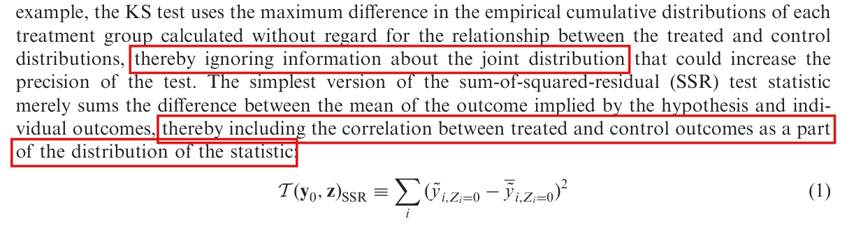
For example, the KS test uses the maximum difference in the empirical cumulative distributions of each treatment group calculated without regard for the relationship between the treated and control distributions, thereby ignoring information about the joint distribution that could increase the precision of the test. The simplest version of the sum-of-squared-residual (SSR) test statistic merely sums the difference between the mean of the outcome implied by the hypothesis and individual outcomes, thereby including the correlation between treated and control outcomes as a part of the distribution of the statistic:

T(y0,z)SSR≡∑i(y~i,Zi=0−y~ˉi,Zi=0)2(1)\mathcal{T}(\mathbf{y}_0,\mathbf{z})_{\mathrm{SSR}}\equiv\sum_i(\tilde y_{i,Z_i=0}-\bar{\tilde y}_{i,Z_i=0})^2 \qquad (1)
The problem

The two sentences give a reason to prefer the simple SSR statistic to the KS statistic: the KS statistic is said to ignore information about the joint distribution of treated and control outcomes, and the SSR statistic is said to include their correlation. This reason does not hold. The statistic meant by equation (1), and computed by the replication code, is the residual sum of squares from the regression of the adjusted outcome on an intercept and the treatment indicator (see P016-E002). It is determined by the group sizes and the first two moments of the adjusted outcome within each treatment group. Like the KS statistic, it is a function of the two group distributions and their sizes, and no pairing of treated with control units and no covariance between them enters either statistic. With the adjusted outcomes and the group sizes fixed, a smaller SSR corresponds exactly to a larger absolute difference in group means. The SSR test is then the test based on the absolute difference in means. A narrower statement is true: the randomization distribution of the SSR statistic reflects the dependence between the two groups that the assignment design induces. The same holds for the randomization distribution of the KS statistic, and the statement does not distinguish the two. The two statistics differ in power because they summarize the two group distributions differently.

Evidence an exact counterexample

I use a derivation and exact finite examples.

Let ai=y~i,Zi=0a_i=\tilde y_{i,Z_i=0} be the adjusted outcomes for one hypothesis, held fixed. Let z∈{0,1}nz\in\{0,1\}^n have n1>0n_1>0 ones and n0>0n_0>0 zeros, with n=n0+n1n=n_0+n_1. I write mgm_g for the mean of aia_i over the units with zi=gz_i=g, mm for the mean over all units, and T(a)=∑i(ai−m)2T(a)=\sum_i(a_i-m)^2. For any group gg and any constant cc, I have

∑i:zi=g(ai−c)2=∑i:zi=g(ai−mg)2+ng(mg−c)2,\sum_{i:z_i=g}(a_i-c)^2=\sum_{i:z_i=g}(a_i-m_g)^2+n_g(m_g-c)^2,

since the cross term vanishes. The least squares fit on an intercept and zz therefore has fitted values m0m_0 and m1m_1, and its residual sum of squares is R(a,z)=∑g∑i:zi=g(ai−mg)2R(a,z)=\sum_g\sum_{i:z_i=g}(a_i-m_g)^2. Taking c=mc=m and summing over the two groups, I obtain T(a)=R(a,z)+n0(m0−m)2+n1(m1−m)2T(a)=R(a,z)+n_0(m_0-m)^2+n_1(m_1-m)^2. Since m0−m=−n1(m1−m0)/nm_0-m=-n_1(m_1-m_0)/n and m1−m=n0(m1−m0)/nm_1-m=n_0(m_1-m_0)/n, I conclude that

R(a,z)=T(a)−n0n1n(m1−m0)2.R(a,z)=T(a)-\frac{n_0n_1}{n}(m_1-m_0)^2.

The term T(a)T(a) and the factor n0n1/nn_0n_1/n do not depend on the assignment. For any two assignments zz and ww with these group sizes, I have R(a,w)≤R(a,z)R(a,w)\le R(a,z) if and only if ∣m1(w)−m0(w)∣≥∣m1(z)−m0(z)∣|m_1(w)-m_0(w)|\ge|m_1(z)-m_0(z)|, ties included. This implies that, for every assignment law PZP_Z on such assignments,

PZ{R(a,Z)≤R(a,zobs)}=PZ{∣m1(Z)−m0(Z)∣≥∣m1(zobs)−m0(zobs)∣}.P_Z\{R(a,Z)\le R(a,z_{\mathrm{obs}})\}=P_Z\{|m_1(Z)-m_0(Z)|\ge|m_1(z_{\mathrm{obs}})-m_0(z_{\mathrm{obs}})|\}.

Further, I have R=n0(q0−m02)+n1(q1−m12)R=n_0(q_0-m_0^2)+n_1(q_1-m_1^2), where qgq_g is the mean of ai2a_i^2 in group gg. The two group distributions and their sizes therefore determine RR.

The table shows the example a=(0,1,2,3)a=(0,1,2,3) with two of the four units treated.

The six assignments of two treated units among four, with a=(0,1,2,3)a=(0,1,2,3) and each assignment of probability 1/61/6. Here δ=m1−m0\delta=m_1-m_0 and n0n1/n=1n_0n_1/n=1, so the SSR equals 5−δ25-\delta^2. The lower-tail pp value of the SSR equals the upper-tail pp value of ∣δ∣|\delta| at every assignment. All values are exact.
Treated unitsδ\deltaT(a)T(a)SSRKSpSSR=p∣δ∣p_{\mathrm{SSR}}=p_{|\delta|}pKSp_{\mathrm{KS}}
1, 2−2-25111/31/31/31/3
1, 3−1-1541/21/22/32/31
1, 40551/21/211
2, 30551/21/211
2, 41541/21/22/32/31
3, 425111/31/31/31/3

Three further exact computations bear on the two printed statements. First, for treated values (0,2)(0,2) and control values (1,3)(1,3), the SSR is 44 and the KS statistic is 1/21/2 whichever control value is paired with which treated value, although the empirical covariance of the pairs, with divisor 22, is 11 under one pairing and −1-1 under the other. Second, both randomization distributions depend on the design: at the assignment that treats units 1 and 2, both pp values are 1/31/3 under complete randomization and 1/21/2 when one unit is chosen uniformly and independently for treatment in each of the blocks {1,3}\{1,3\} and {2,4}\{2,4\}. Third, the SSR is not a function of the KS value: when units 1 and 3 are treated, the KS statistic is 1/21/2 and the SSR is 44, and when units 1 and 4 are treated, the KS statistic is 1/21/2 and the SSR is 55.

What survives

The simple SSR statistic and the validity of its exact randomization test are unaffected by this correction, and no simulation, figure or part of the application depends on this explanation. The SSR and KS statistics remain different summaries with different power (Fig. 2). The statistics with network regressors do use information beyond the two group distributions: in an exact four-unit example, two outcome vectors with the same group distributions have SSR 00 and SSR 44 once degree is added to the regression. I correct only the two explanatory sentences here. I have not recomputed the reported power values.

Corrected

For example, the KS test uses the maximum difference in the empirical cumulative distributions of each treatment group calculated without regard for the relationship between the treated and control distributions, thereby ignoring information about the joint distribution that could increase the precision of the test. The simplest version of the sum-of-squared-residual (SSR) test statistic is the residual sum of squares from a regression of the adjusted outcome on an intercept and treatment. It is determined by the first two empirical moments and the size of each treatment group. With fixed adjusted outcomes and group sizes, smaller SSR values correspond exactly to larger absolute differences in group means. Its sensitivity differs from that of the KS statistic, but it does not acquire pairing information absent from the two group distributions. Adding fixed-network regressors can use information about the alignment of outcomes with the network. The randomization distribution of either statistic also depends on the assignment design.

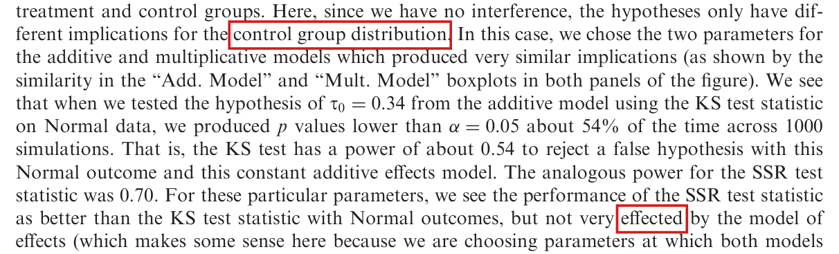
Seven lines of text from page 397, beginning 'example,', followed by displayed equation (1). Red boxes mark the words 'thereby ignoring information about the joint distribution' and the words 'thereby including the correlation between treated and control outcomes as a part of the distribution of the statistic'.
The contrast before equation (1), p. 397; the crop begins after “For”. The marks show the statement that the KS test ignores information about the joint distribution, and the statement that the simplest SSR statistic includes the correlation between treated and control outcomes.

The model behind Fig. 4 uses a similarity exposure from which the unit’s mean exposure among saved assignments with the same own treatment status is subtracted before standardization, not normalized sums of distances; the simulations use a two-sided pp value and reject when it is at most .05.05, and the application uses one-sided pp values.

Section 3, the model that begins “With distance matrix Γ\Gamma”, p. 400 (PDF p. 6); Section 2.2, “less than .05”, p. 400; also p. 398 and the caption of Fig. 3, p. 401

See also under Formal statements (Lean): P016-T3, P016-T4, P016-T6

As printed

With distance matrix Γ\Gamma, Coppock evaluated the model:

y0=yz−β1z−β2g(Γz),\mathbf{y}_0=\mathbf{y}_{\mathbf{z}}-\beta_1\mathbf{z}-\beta_2\colorbox{#ffe58a}{$\displaystyle g(\Gamma\mathbf{z})$},

where gg is a function that normalizes the sums of distances to treated neighbors to have unit variance. This model has a direct effect (β1\beta_1) and an indirect effect (β2\beta_2) that is linear in the distances to treated neighbors. Coppock evaluated this spillover model using the SSR + Design statistic as presented in this article.

Section 2.2, same page: The proportion of pp values from that test less than .05 is plotted in Fig. 3: darker values show fewer rejections, lighter values record more rejections.

The problem

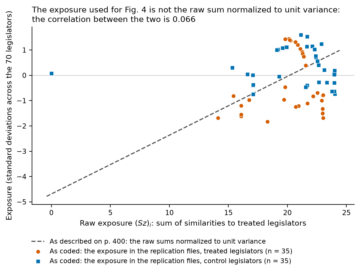
The description of the application does not specify the model to which Fig. 4 and the rectangle on p. 402 refer. In the replication code the matrix is a similarity matrix SS, with Sij=1−∣si−sj∣/2S_{ij}=1-|s_i-s_j|/2 for the W-NOMINATE scores sis_i and sjs_j, so that ideologically closer legislators have larger weights; the diagonal and undefined entries are zero. The exposure of legislator ii is not (Sz)i(Sz)_i normalized to unit variance. The code first subtracts from (Sz)i(Sz)_i its mean over those of 10,000 saved assignments in which legislator ii has the same treatment status, and only then centres and scales across legislators. This subtraction is not a recentring or a rescaling. The exposure used is not an affine function of the raw exposure, even when an intercept and a change in the direct effect are allowed, and in the application table of the replication files the two standardized exposures have correlation 0.070.07. The indirect effect β2\beta_2 of Fig. 4 therefore multiplies a different variable from the one that the text describes, and its sign and its unit can be read only with the coded definition. The regression in the SSR statistic has an intercept, own assignment and this exposure, with no separate degree column, and the phrase “SSR + Design statistic as presented in this article” does not convey this.

The text also does not say how the pp values are formed. The simulations behind Figs. 2 and 3 use a two-sided pp value, twice the smaller of the two tail proportions, capped at 11, and they count a rejection when p≤.05p\le.05. The text and the caption of Fig. 3 say “less than .05”. The application uses one-sided pp values from 500 draws, the lower tail for SSR and the upper tail for KS. The two rules define different tests, and the note does not distinguish them.

Evidence an exact counterexample

I base this correction on the replication code, exact arithmetic on the application table of the replication files, and exact small examples.

Let ri=(Sz)ir_i=(Sz)_i be the raw exposure and hih_i the exposure after the subtraction. If the subtraction could be absorbed by an intercept, the direct effect and a rescaling of the indirect effect, then there would exist constants aa, bb and cc such that hi=a+bzi+crih_i=a+bz_i+cr_i for all ii, and the four columns (1,z,r,h)(1,z,r,h) would have rank at most three. For the first four rows of the application table, the determinant of these four columns, computed in exact rational arithmetic from the decimals of the table, is −1.4030…≠0-1.4030\ldots\ne0. No such constants exist. Across the 70 legislators the correlation between the standardized raw exposure and the standardized exposure used is 0.06650.0665, and the largest difference between the two is 4.764.76 standard deviations.

The same holds in an example in which all assignments are enumerated. Let six units have scores (−1,−3/4,−1/2,0,1/4,1)(-1,-3/4,-1/2,0,1/4,1) and form the pairs (1,2)(1,2), (3,4)(3,4) and (5,6)(5,6), with one treated unit in each pair, a design with eight assignments. At z=(1,0,1,0,1,0)z=(1,0,1,0,1,0) the raw exposures rr and the exposures hh after the subtraction are

r=(9/8, 9/4, 11/8, 17/8, 1, 7/8),h=(5/16, 5/16, 1/8, 1/8, −3/16, −3/16).r=(9/8,\ 9/4,\ 11/8,\ 17/8,\ 1,\ 7/8),\qquad h=(5/16,\ 5/16,\ 1/8,\ 1/8,\ -3/16,\ -3/16).

Units 1 and 2 have equal exposure after the subtraction and unequal raw exposure, while units 1 and 3 differ in both. This implies that hh is not of the form a+cra+cr, and the rank of (1,z,r,h)(1,z,r,h) is four. For the outcome y=(0,1,0,1,1,0)y=(0,1,0,1,1,0) the residual sum of squares is 4/34/3 from the regression on (1,z,h)(1,z,h) and 655/708655/708 from the regression on (1,z,r)(1,z,r).

For the rejection rule, take the reference values 1,2,…,10001,2,\ldots,1000. At the observed value 2525 the lower tail proportion is 1/401/40 and the two-sided pp value of the simulation code is exactly .05.05. The code counts a rejection, and the printed rule does not. At the observed value 4040 the lower tail proportion is .04.04 and the two-sided pp value is .08.08; at 980980 they are .98.98 and .042.042. Neither the one-sided rule nor the two-sided rule rejects whenever the other does.

How pp values are formed and used, in the text and in the replication code. LL and UU are the proportions of the sampled statistics that are at most, and at least, the observed statistic.
TextReplication code
Simulations, pp valuenot statedmin⁡{1,2min⁡(L,U)}\min\{1,2\min(L,U)\}
Simulations, rejectionp<.05p<.05p≤.05p\le.05
Application, pp valuenot statedLL for SSR, UU for KS, 500 draws
Application, bounds of the SSR regionnot statedtransitions in whether the largest pp along the other axis is >.05>.05

The numerical comparison uses the application table that is among the replication files. The data file that the figure script loads is not among them, and I did not recompute Fig. 4.

What survives

This correction changes the description of the model and testing rules used by the replication code. The note’s comparison of a bounded SSR region and an unbounded KS region in Fig. 4 concerns the coded model. I have not established a numerical error in Fig. 4 or in the rectangle, and the absence of a degree column is not shown to make the test invalid. Figs. 2 and 3 are results for the two-sided rule with rejection at p≤.05p\le.05; they cannot be relabelled as results for another rule without recomputation, and my recalculated null rejection rates are compatible with the reported rates of about 4% and 2% within Monte Carlo error; they do not establish a level guarantee. The meaning of β2\beta_2 changes: it is the coefficient of a centred, standardized similarity exposure, not of normalized sums of distances.

Corrected

With similarity matrix SS, where Sij=1−∣si−sj∣/2S_{ij}=1-|s_i-s_j|/2 for the W-NOMINATE scores of legislators i≠ji\ne j and the diagonal and undefined entries are zero, the model evaluated is

y0=yz−β1z−β2e(z),ei(z)=hi(z)−hˉ(z)sh(z),hi(z)=(Sz)i−ziμi1−(1−zi)μi0.\mathbf{y}_0=\mathbf{y}_{\mathbf{z}}-\beta_1\mathbf{z}-\beta_2\colorbox{#ffe58a}{$\displaystyle e(\mathbf{z})$},\qquad \colorbox{#ffe58a}{$\displaystyle e_i(z)=\frac{h_i(z)-\bar h(z)}{s_h(z)}$},\qquad \colorbox{#ffe58a}{$\displaystyle h_i(z)=(Sz)_i-z_i\mu_{i1}-(1-z_i)\mu_{i0}$}.

Here μia\mu_{ia} is the mean of (Sz)i(Sz)_i over those of the 10,000 saved assignments of the matched design in which zi=az_i=a, and hˉ(z)\bar h(z) and sh(z)>0s_h(z)>0 are the mean and the sample standard deviation of hi(z)h_i(z) across the 70 legislators. The indirect effect β2\beta_2 multiplies this centred, standardized similarity exposure, and Fig. 4 and the rectangle on p. 402 refer to this model. For each hypothesis the adjusted outcome u=Y−β1Z−β2e(Z)u=Y-\beta_1Z-\beta_2e(Z) is held fixed. For each reference assignment zz the exposure e(z)e(z) is recomputed, and the SSR statistic is the residual sum of squares from the regression of uu on an intercept, zz and e(z)e(z), with no separate degree column, using the 67 legislators with observed outcomes. The application uses 500 reference assignments drawn from the saved assignments. Its pp value is the proportion of reference statistics that are at most the observed statistic for SSR, and at least the observed statistic for KS. For each axis, the SSR bounds are taken at the second coordinate of each adjacent grid pair where the largest pp value along the other axis changes from at most .05.05 to greater than .05.05, or conversely.

I describe the procedure used for the published figures as follows. Section 2.2: The proportion of pp values from that test less than or equal to .05 is plotted in Fig. 3, where the pp value is twice the smaller of the proportions of sampled statistics that are at most, and at least, the observed statistic, capped at 11. The same descriptive change applies to “lower than α=0.05\alpha=0.05” on p. 398 and to the caption of Fig. 3. This describes the original rule used for Figs. 2 and 3. Figures for the repaired procedure in P016-E008 require recomputation.

Six lines from page 400: the sentence 'With distance matrix Gamma, Coppock evaluated the model:', the displayed model y_0 = y_z - beta_1 z - beta_2 g(Gamma z), and the four lines that follow. Red boxes mark the words 'distance matrix', the term g(Gamma z) in the display, and the words 'normalizes the sums of distances to treated neighbors to have unit variance.'.
The application model, Section 3, p. 400. The marks show the words “distance matrix”, the term g(Γz)g(\Gamma\mathbf{z}) of the model, and the description of gg as a normalization of sums of distances to unit variance.
Five lines of text from page 400. A red box marks the words 'less than .05' in the sentence 'The proportion of p values from that test less than .05 is plotted in Fig. 3'.
Section 2.2, p. 400. The mark shows the rejection rule of the simulations as printed, “less than .05”.
Scatter plot. Horizontal axis: raw exposure (Sz)_i, the sum of similarities to treated legislators, from 0 to 25. Vertical axis: exposure in standard deviations across the 70 legislators, from -5 to 2. A dashed grey line rising from about -4.8 at raw exposure 0 to about 1 at raw exposure 24 shows the raw sums centred and scaled to unit sample variance, labelled as described on page 400. Orange circles (35 treated legislators) and blue squares (35 control legislators) show the exposure in the replication files, labelled as coded. The points form a cloud between raw exposures 14 and 24 and between -1.9 and 1.6 on the vertical axis, with no visible linear relation to the dashed line; at raw exposure 0 and vertical value near 0, a blue square covers an orange circle at the same position. The title reads 'The exposure used for Fig. 4 is not the raw sum normalized to unit variance: the correlation between the two is 0.066'.
The exposure used in the application against the raw exposure, for the 70 legislators of the application table in the replication files. If p. 400’s normalization is read as centring and scaling the raw similarity sum (Sz)i(Sz)_i to unit sample variance, the points would lie on the dashed line. The correlation between the two standardized exposures is 0.06650.0665. Two legislators have raw exposure 00 and identical standardized exposure; their symbols overlap.

Minor (9)

Real but inconsequential, for example a misprint that does not change a result.

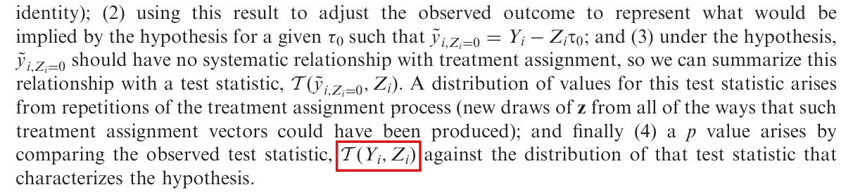
In step (4) the observed test statistic is T(y~i,Zi=0,Zi)\mathcal{T}(\tilde y_{i,Z_i=0},Z_i), computed from the outcome adjusted under the hypothesis, and not T(Yi,Zi)\mathcal{T}(Y_i,Z_i).

Section 1, second paragraph, step (4), p. 396 (PDF p. 2)

See also under Formal statements (Lean): P016-T7, P016-T8

As printed

(2) using this result to adjust the observed outcome to represent what would be implied by the hypothesis for a given τ0\tau_0 such that y~i,Zi=0=Yi−Ziτ0\tilde y_{i,Z_i=0}=Y_i-Z_i\tau_0; and (3) under the hypothesis, y~i,Zi=0\tilde y_{i,Z_i=0} should have no systematic relationship with treatment assignment, so we can summarize this relationship with a test statistic, T(y~i,Zi=0,Zi)\mathcal{T}(\tilde y_{i,Z_i=0},Z_i). A distribution of values for this test statistic arises from repetitions of the treatment assignment process (new draws of z\mathbf{z} from all of the ways that such treatment assignment vectors could have been produced); and finally (4) a pp value arises by comparing the observed test statistic, T(Yi,Zi)\colorbox{#ffe58a}{$\mathcal{T}(Y_i,Z_i)$} against the distribution of that test statistic that characterizes the hypothesis.

The problem

Steps (2) and (3) define the adjusted outcome y~i,Zi=0=Yi−Ziτ0\tilde y_{i,Z_i=0}=Y_i-Z_i\tau_0 and build the randomization distribution from it. Step (4) then writes the observed statistic with the raw outcome YiY_i. In general T(Y,Z)\mathcal{T}(Y,Z) differs from T(y~,Z)\mathcal{T}(\tilde y,Z); the two coincide when τ0=0\tau_0=0 or when the statistic is unchanged by the adjustment. As printed, the observed statistic is then compared with the distribution of a different quantity. Steps (2) and (3) show which statistic is meant, and the replication code computes it.

Evidence an exact counterexample

The evidence is a derivation, an exact counterexample to the rule as printed, and a check of the replication code.

Let ZZ be the realized assignment and YY the vector of observed outcomes. Suppose that the hypothesis yi,Zi=1=yi,Zi=0+τ0y_{i,Z_i=1}=y_{i,Z_i=0}+\tau_0 holds, with no interference. Inserting it into the identity Yi=Ziyi,Zi=1+(1−Zi)yi,Zi=0Y_i=Z_iy_{i,Z_i=1}+(1-Z_i)y_{i,Z_i=0}, I obtain Yi=yi,Zi=0+τ0ZiY_i=y_{i,Z_i=0}+\tau_0Z_i. This implies that ui=Yi−τ0Ziu_i=Y_i-\tau_0Z_i equals yi,Zi=0y_{i,Z_i=0}, which does not depend on the assignment. Under the hypothesis, the statistic at the realized assignment is T(u,Z)\mathcal{T}(u,Z), and its randomization distribution is that of T(u,Z′)\mathcal{T}(u,Z'), where Z′Z' follows the assignment law of the experiment and uu is held fixed. For the difference in means, I have T(Y,Z)=T(u,Z)+τ0\mathcal{T}(Y,Z)=\mathcal{T}(u,Z)+\tau_0.

For the counterexample, I take four units, two of them treated, with the six assignments equally likely, u=(0,1,2,3)u=(0,1,2,3), true effect τ0=10\tau_0=10, and the difference in means as the statistic. The six values of T(u,Z′)\mathcal{T}(u,Z') are −2,−1,0,0,1,2-2,-1,0,0,1,2. At Z=(0,0,1,1)Z=(0,0,1,1) the observed outcomes are Y=(0,1,12,13)Y=(0,1,12,13), the raw statistic is 1212, and the adjusted statistic is 22. The two-sided pp value is the proportion of the six values of T(u,Z′)\mathcal{T}(u,Z') that are at least as large in absolute value as the observed statistic. It is 00 for the raw statistic and 1/31/3 for the adjusted statistic. Under each of the six assignments the raw statistic lies between 88 and 1212, and its pp value is 00. The rule as printed rejects the true hypothesis τ0=10\tau_0=10 with probability one.

The randomization routine of the replication code adjusts the outcome once, evaluates the observed statistic on the adjusted outcome, and compares it with the statistic evaluated on the same adjusted outcome under the sampled assignments.

What survives

The procedure of steps (1) to (3) and the inspected randomization routine are unchanged. I found no reported result that depends on the raw statistic. Only the symbol in step (4) changes.

Corrected

(4) a pp value arises by comparing the observed test statistic, T(y~i,Zi=0,Zi)\colorbox{#ffe58a}{$\mathcal{T}(\tilde y_{i,Z_i=0},Z_i)$}, evaluated at the realized assignment, against the distribution of that test statistic that characterizes the hypothesis.

In full: let YY be the vector of observed outcomes, ZZ the observed assignment and ui=Yi−τ0Ziu_i=Y_i-\tau_0Z_i the outcome adjusted under the hypothesized additive effect τ0\tau_0. Compare the observed T(u,Z)\mathcal{T}(u,Z) with the distribution of T(u,Z′)\mathcal{T}(u,Z'), where Z′Z' follows the experimental assignment law and uu is held fixed.

Eight lines of text from page 396 that give steps (2), (3) and (4) of the testing procedure. A red box marks the expression T(Y_i, Z_i) in the words 'comparing the observed test statistic, T(Y_i, Z_i) against the distribution of that test statistic'.
Steps (2) to (4) of the testing procedure, p. 396. The mark shows the observed test statistic of step (4), printed with the raw outcome YiY_i.

The three displayed definitions of the test statistics need the absolute value in the KS statistic, the mean of the unit’s own assignment group in equation (1), and the row index and the intercept in equation (2).

Footnote 3, p. 396 (PDF p. 2); equation (1) and the sentence before it, p. 397 (PDF p. 3); equation (2) and the sentence before it, p. 399 (PDF p. 5)

See also under Formal statements (Lean): P016-T5, P016-T9, P016-T10

As printed

Footnote 3, p. 396: If the empirical cumulative distribution function (ECDF) of the treated units is F1F_1 and the ECDF of the control units is F0F_0, then the KS test statistic is T(y0,z)KS=max⁡i=1,…,n[F1(yi,0)−F0(yi,0)]\mathcal{T}(\mathbf{y}_0,\mathbf{z})_{\mathrm{KS}}=\max_{i=1,\ldots,n}\colorbox{#ffe58a}{$[F_1(y_{i,0})-F_0(y_{i,0})]$}, where F(x)=(1/n)∑i=1nI(xi≤x)F(x)=(1/n)\sum_{i=1}^{n}I(x_i\le x) records the proportion of the distribution of xx at or below xix_i (Hollander 1999, section 5.4).

p. 397: The simplest version of the sum-of-squared-residual (SSR) test statistic merely sums the difference between the mean of the outcome implied by the hypothesis and individual outcomes, thereby including the correlation between treated and control outcomes as a part of the distribution of the statistic:

T(y0,z)SSR≡∑i(y~i,Zi=0−y~‾i,Zi=0)2(1)\mathcal{T}(\mathbf{y}_0,\mathbf{z})_{\mathrm{SSR}}\equiv\sum_i(\tilde y_{i,Z_i=0}-\colorbox{#ffe58a}{$\displaystyle \overline{\tilde y}_{i,Z_i=0}$})^2 \qquad (1)

p. 399: If we collected ZiZ_i, zTS\mathbf{z}^{T}\mathbf{S}, and 1TS\mathbf{1}^{T}\mathbf{S} into a matrix X\mathbf{X}, and fit the y~i,Zi=0\tilde y_{i,Z_i=0} as a linear function of X\mathbf{X} with fitted coefficients β^\hat{\boldsymbol{\beta}} then we could define the test statistic as

T(y0,z)SSR≡∑i(y~i,Zi=0−Xβ^)2.(2)\mathcal{T}(y_0,\mathbf{z})_{\mathrm{SSR}}\equiv\sum_i(\tilde y_{i,Z_i=0}-\colorbox{#ffe58a}{$\displaystyle \mathbf{X}\hat{\boldsymbol{\beta}}$})^2. \qquad (2)
The problem

Read literally, the KS display differs from the statistic used, equation (1) leaves its mean undefined, and equation (2) omits the component index of its fitted vector.

  1. Footnote 3 has no absolute value, and the display is the one-sided statistic max⁡i{F1−F0}\max_i\{F_1-F_0\}. The statistic described, which is sensitive to any difference between the two distributions, and the statistic coded are the two-sided max⁡i∣F1−F0∣\max_i|F_1-F_0|.
  2. In equation (1) the overbar carries the unit index ii and is not defined. The statistic meant is the residual sum of squares from the regression of the adjusted outcome on an intercept and zz, in which the mean subtracted from unit ii is the mean of its own assignment group. If the overbar is read as the mean over all units, the display is the total sum of squares, which does not depend on z\mathbf{z}. The sentence before the display says “sums the difference” where the squared difference is meant.
  3. In equation (2) the summand subtracts the whole vector Xβ^\mathbf{X}\hat{\boldsymbol{\beta}} from the scalar y~i,Zi=0\tilde y_{i,Z_i=0}, since the row index is missing. The list of columns of X\mathbf{X} has no constant. The regression in the replication code has an intercept.

The surrounding text on least squares regression identifies the statistics that are meant.

Evidence an exact counterexample

The evidence is exact arithmetic on small examples, a derivation, and a check of the functions in the replication code on the same examples.

For the KS statistic, let the adjusted outcomes be u=(0,1,2,3)u=(0,1,2,3), with z=(0,0,1,1)z=(0,0,1,1). At the points 0,1,2,30,1,2,3 the differences F1−F0F_1-F_0 are −1/2,−1,−1/2,0-1/2,-1,-1/2,0. The display as printed gives 00, and the two-sided statistic is 11.

For equation (1), an intercept and zz fit one constant cgc_g to each assignment group gg. For any constant cc, I have ∑i:zi=g(ui−c)2=∑i:zi=g(ui−uˉg)2+ng(uˉg−c)2\sum_{i:z_i=g}(u_i-c)^2=\sum_{i:z_i=g}(u_i-\bar u_g)^2+n_g(\bar u_g-c)^2, where uˉg\bar u_g is the mean of the ngn_g units of group gg. The fitted constants are therefore the group means, and the residual sum of squares is ∑i(ui−uˉzi)2\sum_i(u_i-\bar u_{z_i})^2. With u=(0,1,2,3)u=(0,1,2,3) and two of the four units treated, the total sum of squares is 55 under all six assignments, and the residual sum of squares takes the values 1,4,5,5,4,11,4,5,5,4,1. At the assignment that treats units 1 and 2, the lower-tail pp value is 1/31/3 for the residual sum of squares and 11 for the total sum of squares.

For equation (2), take six units with the single edge {1,2}\{1,2\}, z=(1,0,1,0,1,0)z=(1,0,1,0,1,0) and u=(1,1,1,1,1,1)u=(1,1,1,1,1,1). The residual sum of squares is 00 with the intercept and 22 without it.

On these inputs the functions of the replication code return 11 for the KS statistic, 1,4,5,5,4,11,4,5,5,4,1 for the simple SSR statistic and 00 for the network SSR statistic. These are the values of the corrected definitions.

What survives

The inspected functions of the replication code compute the corrected definitions. These notation repairs do not change their outputs, and I found no error in the comparisons of Figs. 2 to 4 caused by these defects. Note that the signed maximum of footnote 3 is a valid one-sided statistic; it is not the statistic used. The power recalculations are described below under what I checked.

Corrected

Write ui=y~i,Zi=0u_i=\tilde y_{i,Z_i=0}. For g∈{0,1}g\in\{0,1\}, let ng=#{i:zi=g}>0n_g=\#\{i:z_i=g\}>0, let uˉg=ng−1∑i:zi=gui\bar u_g=n_g^{-1}\sum_{i:z_i=g}u_i, and let Fg(t)=ng−1∑i:zi=gI(ui≤t)F_g(t)=n_g^{-1}\sum_{i:z_i=g}I(u_i\le t).

Footnote 3:

T(y0,z)KS=max⁡i=1,…,n∣F1(ui)−F0(ui)∣=sup⁡t∣F1(t)−F0(t)∣.\mathcal{T}(\mathbf{y}_0,\mathbf{z})_{\mathrm{KS}}=\max_{i=1,\ldots,n}\colorbox{#ffe58a}{$\displaystyle |$}F_1(u_i)-F_0(u_i)\colorbox{#ffe58a}{$\displaystyle |$}=\sup_t|F_1(t)-F_0(t)|.

Equation (1): The simplest version of the sum-of-squared-residual (SSR) test statistic sums the squared differences between individual outcomes and the mean of the outcome in the unit’s own assignment group:

T(y0,z)SSR≡∑i(ui−uˉzi)2.(1)\mathcal{T}(\mathbf{y}_0,\mathbf{z})_{\mathrm{SSR}}\equiv\sum_i(u_i-\colorbox{#ffe58a}{$\displaystyle \bar u_{z_i}$})^2. \qquad (1)

Equation (2): Let X(z)\mathbf{X}(\mathbf{z}) be the matrix with rows xiT=(1,zi,(zTS)i,(1TS)i)x_i^{T}=(\colorbox{#ffe58a}{$1$},z_i,(\mathbf{z}^{T}\mathbf{S})_i,(\mathbf{1}^{T}\mathbf{S})_i), and let β^\hat{\boldsymbol{\beta}} be a least squares coefficient vector. Then

T(y0,z)SSR≡min⁡b∥u−X(z)b∥22=∑i{ui−(X(z)β^)i}2.(2)\mathcal{T}(\mathbf{y}_0,\mathbf{z})_{\mathrm{SSR}}\equiv\min_b\|u-\mathbf{X}(\mathbf{z})b\|_2^2=\sum_i\{u_i-\colorbox{#ffe58a}{$\displaystyle (\mathbf{X}(\mathbf{z})\hat{\boldsymbol{\beta}})_i$}\}^2. \qquad (2)
Footnotes 2, 3 and 4 of page 396. In footnote 3, a red box marks the bracketed expression F_1(y_i,0) - F_0(y_i,0) that follows 'max over i = 1,...,n' in the definition of the KS test statistic.
Footnotes 2 to 4, p. 396. The mark shows the difference of the two ECDFs in the KS statistic of footnote 3, printed in square brackets without an absolute value.
Four lines of text followed by displayed equation (1), T(y_0, z)_SSR defined as the sum over i of (y-tilde_i,Zi=0 minus y-tilde-bar_i,Zi=0) squared. Red boxes mark the words 'sums the difference' in the text and the overbarred term y-tilde-bar_i,Zi=0 in the equation.
The sentence that introduces equation (1), and equation (1), p. 397. The marks show the words “sums the difference” and the mean that is subtracted in the summand.
Four lines of text followed by displayed equation (2), T(y_0, z)_SSR defined as the sum over i of (y-tilde_i,Zi=0 minus X beta-hat) squared. Red boxes mark the words 'Z_i, z-transpose S, and 1-transpose S into a matrix X,' in the text and the term X beta-hat in the equation.
The sentence that introduces equation (2), and equation (2), p. 399. The marks show the list of columns of X\mathbf{X}, which has no constant, and the fitted vector Xβ^\mathbf{X}\hat{\boldsymbol{\beta}}, printed without a row index.

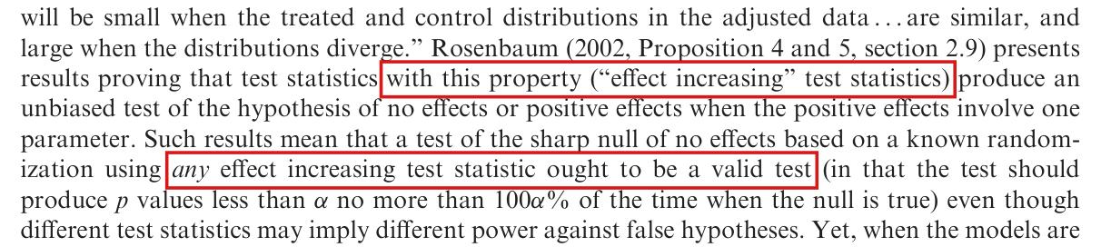
A statistic that is small when the two distributions are similar and large when they diverge need not be “effect increasing”, and a randomization test of a sharp null hypothesis is valid for any test statistic, with or without that property.

Section 1, last paragraph, the two sentences after the quotation, p. 397 (PDF p. 3); the quotation begins on p. 396

See also under Formal statements (Lean): P016-T8, P016-T11, P016-T12, P016-T14

As printed

“Select a test statistic [T\mathcal{T}] that will be small when the treated and control distributions in the adjusted data … are similar, and large when the distributions diverge.” Rosenbaum (2002, Proposition 4 and 5, section 2.9) presents results proving that test statistics with this property (“effect increasing” test statistics) produce an unbiased test of the hypothesis of no effects or positive effects when the positive effects involve one parameter. Such results mean that a test of the sharp null of no effects based on a known randomization using any effect increasing test statistic ought to be a valid test (in that the test should produce pp values less than α\alpha no more than 100α%100\alpha\% of the time when the null is true) even though different test statistics may imply different power against false hypotheses.

The problem

The passage identifies the property in the quotation, being small for similar distributions and large for divergent ones, with the effect increasing property. The two are different. A statistic is effect increasing if, at a fixed assignment, raising treated responses and lowering control responses cannot decrease it. This condition is directional. An unsigned measure of the difference between two distributions need not satisfy it, and the two-sided KS statistic does not. The next sentence gives a correct sufficient condition for validity, but validity holds for every test statistic calibrated under the known assignment law, and whether a test is unbiased against alternatives is a separate question.

Evidence an exact counterexample

The evidence is an exact counterexample and a derivation.

Fix the assignment z=(1,1,0,0)z=(1,1,0,0) and change y=(0,1,2,3)y=(0,1,2,3) to y′=(2,3,2,3)y'=(2,3,2,3). Both treated responses rise by 22 and the control responses are unchanged. The two-sided KS statistic is 11 for yy, where every treated value lies below every control value, and 00 for y′y', where both groups have the values 22 and 33. Since the statistic decreases, it is not effect increasing. The KS function of the replication code returns the same two values, and the signed maximum printed in footnote 3 also falls from 11 to 00.

For validity, let Ω\Omega be the finite set of assignments, with known probabilities q(z)>0q(z)>0. Under the sharp null hypothesis of no effects, the outcome vector y0y^0 is the same under every assignment. Any statistic then has fixed scores s(z)=T(y0,z)s(z)=\mathcal{T}(y^0,z). Define the pp value p(z)=∑w∈Ω:s(w)≥s(z)q(w)p(z)=\sum_{w\in\Omega:s(w)\ge s(z)}q(w). Let v1>⋯>vkv_1>\cdots>v_k be the distinct scores, let mjm_j be the probability that s(Z)=vjs(Z)=v_j, and let Mj=m1+⋯+mjM_j=m_1+\cdots+m_j. An assignment with score vjv_j has p(z)=Mjp(z)=M_j, and MjM_j is strictly increasing in jj. Fix α∈[0,1]\alpha\in[0,1]. If M1>αM_1>\alpha, the event {p(Z)≤α}\{p(Z)\le\alpha\} is empty. Otherwise, let rr be the largest index such that Mr≤αM_r\le\alpha. Then the event consists of the assignments with scores v1,…,vrv_1,\ldots,v_r, and its probability is Mr≤αM_r\le\alpha. I conclude that Pr⁡{p(Z)≤α}≤α\Pr\{p(Z)\le\alpha\}\le\alpha for every statistic. The argument does not use the effect increasing property.

The cited propositions and the quotation were not compared with the two works cited.

What survives

The conclusion that the randomization test of the sharp null hypothesis is valid stands, for a more general reason. Nothing later in the note uses the effect increasing property: the statistics, the simulations and the application are unaffected, and the note does not claim that its SSR statistics are effect increasing. Only these explanatory sentences change.

Corrected

A statistic is effect increasing if increasing treated responses and decreasing control responses, at fixed assignment, cannot decrease it. The quoted advice about distributional divergence does not imply this directional condition. Under a sharp null hypothesis, calibrating any specified test statistic under the known assignment law gives a valid test; unbiasedness against alternatives is a separate question.

Eight lines of text from the top of page 397. Red boxes mark the words 'with this property ("effect increasing" test statistics)' and the words 'any effect increasing test statistic ought to be a valid test'.
The end of the quotation and the two sentences that follow it, p. 397. The first mark shows the mistaken identification of the quoted property with “effect increasing”. The second marks a sufficient validity statement, whose conclusion remains correct.

The text describes the simulation behind Fig. 3 as 10,000 experiments of 1000 sampled permutations each, and the replication code defaults to 1000 experiments of 10,000 sampled assignments each; which setting produced the published figure is not known.

Section 2.2, first and second paragraphs, p. 400 (PDF p. 6)

As printed

For each test statistic, we tested the hypothesis τ=τ0, β=τ0\tau=\tau_0,\ \beta=\tau_0 by using a simulated permutation test: we sampled 1000 permutations. We executed that test 10,000 times for each pair of parameters.

Again, all of the tests are valid in the sense of rejecting the truth no more than 5% of the time when α=.05\alpha=.05 although all of these tests are conservative: the SSR-based tests rejected the truth roughly 4% of the 10,000 simulations but the KS tests rejected the truth roughly 2% of the time.

The problem

The text and the replication code disagree about how the simulation behind Fig. 3 is divided. In the code, when no setting is supplied, the number of simulated experiments is 1000 and each test samples 10,000 assignments, and the driver files of the archive supply no other setting. The environment variable that the code provides changes only the number of experiments; with 10,000 experiments each test still samples 10,000 assignments, which again differs from the text. Since saved results and run logs are not among the replication files, the setting used for the published figure cannot be recovered. The difference bears on the precision of the reported rates: at a rejection rate of 0.040.04 the Monte Carlo standard error is 0.00620.0062 with 1000 experiments and 0.00200.0020 with 10,000.

Evidence a recalculation from the source

The evidence is a recalculation from the replication code and a check of the page. Running the count expressions, the sampler and the test routine of both released versions of the code, I obtain a matrix of 1000 assignments of the 256 units, and each test receives 10,000 samples. The standard errors are p(1−p)/N\sqrt{p(1-p)/N} at p=1/25p=1/25, which is 0.0061970.006197 for N=1000N=1000 and 0.0019600.001960 for N=10,000N=10{,}000. I obtained these counts from the code settings and calls, without simulating rejection rates.

What survives

No rejection rate, power comparison or conclusion is shown to be wrong. The discrepancy establishes that the text and the code disagree, and it does not establish which setting was run. Fig. 2 is unaffected, since its script sets 1000 sampled assignments itself, and so are the statistics, the framework and the application.

Corrected

The deposited driver for Fig. 3 defaults to 1,000 simulated experiments with 10,000 sampled assignments for each permutation distribution. This allocation differs from the 10,000 experiments with 1,000 sampled permutations described on p. 400. The counts used to produce the published figure cannot be recovered from the deposited files, because saved results and run logs are not supplied; the published counts should be reconciled against the original invocation and results.

Four lines of text from page 400. A red box marks the words 'we sampled 1000 permutations. We executed that test 10,000 times'.
Section 2.2, first paragraph, p. 400. The mark shows the description of the simulation: 1000 sampled permutations for each test, and 10,000 tests for each pair of parameters.
Four lines of text from page 400. A red box marks the words 'of the 10,000 simulations' in 'the SSR-based tests rejected the truth roughly 4 percent of the 10,000 simulations but the KS tests rejected the truth roughly 2 percent of the time'.
Section 2.2, second paragraph, p. 400. The mark shows the number of simulations to which the rejection rates of about 4% and 2% are referred.

The printed rule, which rejects when p<.05p<.05, is valid at level .05.05; the simulation code rejects when p≤.05p\le.05 with tail proportions that do not count the observed statistic, and that rule can have size slightly above .05.05.

Section 2.2, first two paragraphs, p. 400 (PDF p. 6), with the validity statement on p. 397 (PDF p. 3); the rejection rule is in the simulation scripts of the replication files

See also under Formal statements (Lean): P016-T13, P016-T14, P016-T21

As printed

The proportion of pp values from that test less than .05 is plotted in Fig. 3: darker values show fewer rejections, lighter values record more rejections. All of these test statistics are valid—they reject the true null of τ=.5, β=2\tau=.5,\ \beta=2 no more than 5% of the time at α=.05\alpha=.05—and the plots are darkest in the area where the two lines showing the true parameters intersect.

Simulation scripts of the replication files: m <- m <= ALPHA, with ALPHA <- 0.05.

The problem

The validity statements on pp. 397 and 400 are correct for the rule as printed. With a fixed statistic and BB fresh reference draws, the rule that rejects when the pp value is less than .05.05 has null rejection probability at most 50/100150/1001 for B=1000B=1000 and at most 500/10001500/10001 for B=10,000B=10{,}000. The simulation code applies a different rule. Each tail is the proportion of the BB reference statistics that are at most, or at least, the observed statistic, and the observed statistic is not counted among them. The pp value is twice the smaller tail, capped at 11, and a rejection is counted when p≤.05p\le.05. This rule is not a test of level .05.05 in general: its size can exceed .05.05 slightly, and its pp value can equal 00.

Evidence an exact counterexample

The evidence is an exact counterexample, computed by enumeration and rational arithmetic, and a derivation.

For the counterexample, I take sixteen units, eight of them treated, with all (168)=12870\binom{16}{8}=12870 assignments equally likely, the sharp null hypothesis of no effect with outcomes 2i2^i for i=0,…,15i=0,\ldots,15, and the simple SSR statistic. The statistic takes 6435 distinct values over these assignments, each shared by an assignment and its complement. The observed assignment and the BB reference assignments are drawn independently from the design.

Exact null rejection probability at nominal level .05.05 in the sixteen-unit example, rounded to six decimals.
Reference draws BBCoded rule, p≤.05p\le.05Printed rule, p<.05p<.05
100010000.0517930.0517930.0497950.049795
10,00010{,}0000.0500400.0500400.0498400.049840

The probability that the coded pp value equals 00 is 0.00180.0018 for B=1000B=1000.

For the derivation, let T0T_0 be the observed statistic and T1,…,TBT_1,\ldots,T_B the reference statistics, and suppose that these B+1B+1 statistics are exchangeable under the null hypothesis. Set L=#{b:Tb≤T0}L=\#\{b:T_b\le T_0\} and U=#{b:Tb≥T0}U=\#\{b:T_b\ge T_0\}. With ties broken at random, the rank of T0T_0 among the B+1B+1 statistics is uniform on {1,…,B+1}\{1,\ldots,B+1\}, and this rank is at most L+1L+1. I therefore have Pr⁡(L≤c)≤(c+1)/(B+1)\Pr(L\le c)\le(c+1)/(B+1) for every integer c≥0c\ge0, and the same bound for UU. The event 2min⁡(L,U)/B<α2\min(L,U)/B<\alpha requires that L≤cL\le c or U≤cU\le c with c=⌈αB/2⌉−1c=\lceil\alpha B/2\rceil-1, and by the union bound its probability is at most 2(c+1)/(B+1)2(c+1)/(B+1). At α=.05\alpha=.05 and B=1000B=1000, I have c=24c=24, and the bound is 50/1001<.0550/1001<.05. The coded rule allows c=⌊αB/2⌋=25c=\lfloor\alpha B/2\rfloor=25, for which the same bound is 52/1001>.0552/1001>.05; the counterexample shows that the size can exceed .05.05. Next, set pL=(1+L)/(B+1)p_L=(1+L)/(B+1) and pU=(1+U)/(B+1)p_U=(1+U)/(B+1). For every a∈[0,1]a\in[0,1], I have Pr⁡(pL≤a)=Pr⁡(L+1≤⌊a(B+1)⌋)≤⌊a(B+1)⌋/(B+1)≤a\Pr(p_L\le a)=\Pr(L+1\le\lfloor a(B+1)\rfloor)\le\lfloor a(B+1)\rfloor/(B+1)\le a, and the same holds for pUp_U. For α<1\alpha<1 the event min⁡{1,2min⁡(pL,pU)}≤α\min\{1,2\min(p_L,p_U)\}\le\alpha is the union of {pL≤α/2}\{p_L\le\alpha/2\} and {pU≤α/2}\{p_U\le\alpha/2\}. Its probability is at most α\alpha.

What survives

The validity statement for the exact randomization test on p. 397 and the printed rule at level .05.05 stand, as do the statistics and the framework. No reported rejection rate, power ranking or figure is shown to change. Note that the counterexample is a constructed design of sixteen units and not the simulation of 256 units in the note, and the excess over .05.05 is a fraction of a percentage point. The pp values of the application are computed from a fixed saved set of assignments; they need a separate argument and were not examined here.

Corrected

The validity statement on p. 397 stands. For a repaired simulation procedure with the existing tail estimator, 1,000 or 10,000 independent reference draws and a fixed statistic, count a rejection when p < .05p\,\colorbox{#ffe58a}{$<$}\,.05. The published Figs. 2 and 3 describe the original p≤.05p\le.05 rule (P016-E006); they have not been recomputed for the repaired procedure. Figures for the repaired procedure require recomputation.

For a pp value that is valid at every threshold, let LL and UU be the numbers of the BB reference statistics that are at most, and at least, the observed statistic, and set

pL=1+LB+1,pU=1+UB+1,p=min⁡{1,2min⁡(pL,pU)}.p_L=\frac{\colorbox{#ffe58a}{$\displaystyle 1+$}L}{B\colorbox{#ffe58a}{$\displaystyle +1$}},\qquad p_U=\frac{\colorbox{#ffe58a}{$\displaystyle 1+$}U}{B\colorbox{#ffe58a}{$\displaystyle +1$}},\qquad p=\min\{1,2\min(p_L,p_U)\}.

If the observed statistic and the BB reference statistics are exchangeable under the null hypothesis, as they are for a fixed statistic and independent draws from the assignment law, then Pr⁡(p≤α)≤α\Pr(p\le\alpha)\le\alpha for every α∈[0,1]\alpha\in[0,1]. Sampling from a fixed saved set of assignments, as in the application, requires a separate justification of exchangeability.

Seven lines of text from page 400. Red boxes mark the words 'less than .05' and the sentence part 'All of these test statistics are valid - they reject the true null of tau = .5, beta = 2 no more than 5 percent of the time at alpha = .05 -'.
Section 2.2, first paragraph, p. 400. The marks show the rejection rule as printed, “less than .05”, and the statement that all six tests reject the true null no more than 5% of the time at α=.05\alpha=.05. The statement is correct for the rule as printed; the simulation code applies a different rule.

The application script saves, as the upper endpoint of an interior accepted range, the first rejected grid point and not the last accepted one; the pp values, Fig. 4 and the printed rectangle are not shown to depend on this.

Section 3, last sentence, p. 402 (PDF p. 8); the endpoint helper find_breaks is in the application script of the replication files, lines 12–18, 77–78 and 83–84

As printed

it would be very unlikely that the data were generated from the model with parameters outside the rectangle with corners (−0.6,0.2)(-0.6, 0.2) and (0.3,−0.4)(0.3, -0.4).

Helper find_breaks of CoppockJEPS_figure2code.R, the application script of the replication files:

breaks[i+1] <- x[i]!=x[i+1]

return(which(breaks))

In the main part of the script, and likewise for the indirect effect:

direct_breaks <- find_breaks(apply(pmat.ssr, MARGIN=1, FUN=max) >.05)

directs.95.2 <- directs[direct_breaks]

The problem

The helper find_breaks returns the positions that follow each change of the accepted or rejected indicator along a grid axis, and the script uses those positions as the endpoints of the accepted range. For a run of accepted grid points at positions r,…,sr,\ldots,s strictly inside the grid, the helper returns rr and s+1s+1. The lower endpoint is right. The upper endpoint is the first rejected grid point, one step above the last accepted one; the step is 2/49≈0.042/49\approx0.04 on the grid of 50 points over [−1,1][-1,1]. The defect is in the endpoint summaries that the script saves. The rectangle on p. 402 is rounded text in the manuscript source, and it is not shown to come from these endpoints.

Evidence an exact counterexample

I checked the derivation and an exact counterexample using the original code.

Let aia_i indicate that the largest pp value in row ii of the matrix exceeds .05.05, for i=1,…,ni=1,\ldots,n. The helper sets entry i+1i+1 of its output to the truth value of ai≠ai+1a_i\ne a_{i+1} for i=1,…,n−1i=1,\ldots,n-1, and it returns the positions of the true entries. If the accepted positions are exactly r,…,sr,\ldots,s with 1<r≤s<n1<r\le s<n, then the changes occur at i=r−1i=r-1 and at i=si=s, and the helper returns (r,s+1)(r,s+1). The script then saves the grid values (gr,gs+1)(g_r,g_{s+1}). The extremes of the accepted grid values are (gr,gs)(g_r,g_s). On the grid of the script, gi=(2i−51)/49g_i=(2i-51)/49, which implies that gs+1−gs=2/49g_{s+1}-g_s=2/49.

For the counterexample, let the 50×5050\times50 matrix have pij=1/10p_{ij}=1/10 for 20≤i≤3020\le i\le30 and 22≤j≤2722\le j\le27, and pij=1/50p_{ij}=1/50 elsewhere. The accepted direct range is positions 20 to 30, that is [−11/49,9/49][-11/49,9/49], and the script saves positions 20 and 31, that is [−11/49,11/49][-11/49,11/49]. The accepted indirect range is positions 22 to 27, that is [−1/7,3/49][-1/7,3/49], and the script saves positions 22 and 28, that is [−1/7,5/49][-1/7,5/49]. The helper returns rr and s+1s+1 for each of the 1176 interior runs of the grid. I did not recompute the application’s pp-value matrices to establish this endpoint error.

What survives

The two matrices of pp values, the shading and the axes of Fig. 4, and the contrast between a bounded SSR region and a KS region that reaches the edges of the grid are computed before this step and do not use it. The correction changes only the saved endpoint summaries: for an interior run, the upper endpoint falls by 2/492/49. It does not establish corrected values for the rounded rectangle on p. 402.

Corrected

For each parameter, the endpoints of the accepted range are the extremes of the grid coordinates whose projected pp value exceeds .05.05, that is range(grid[accepted]) in place of the transition positions, and an empty accepted set is reported as empty. When a projection is accepted at positions r,…,sr,\ldots,s, its endpoints are the grid coordinates grg_r and gs\colorbox{#ffe58a}{$g_s$}, not grg_r and gs+1g_{s+1}. If the accepted set is not connected, the product of the two ranges is a bounding rectangle and not the accepted set itself. This corrects the endpoint extraction only; it does not alter the matrices of pp values or establish corrected values for the rounded rectangle on p. 402.

Five lines of text from page 402. A red box, in two parts across a line break, marks the words 'outside the rectangle with corners (-0.6, 0.2) and (0.3, -0.4).'.
Section 3, last sentence, p. 402. The mark shows the rectangle that summarizes the SSR region. The defect is in the endpoint summaries that the application script saves; the printed rectangle is not shown to come from them.

Six local corrections: the hypotheses of Fig. 2 differ in what they imply for the treated group, the ECDF threshold in footnote 3 is xx, the joint hypothesis on p. 400 is τ=τ0\tau=\tau_0, β=β0\beta=\beta_0, the chamber is the New Mexico House of Representatives, two reference entries misstate names, and three words are misprinted.

Last paragraph of p. 398 (PDF p. 4); also footnote 3, p. 396; p. 399; p. 400; the reference list, pp. 402–403; and the abstract, p. 395

See also under Formal statements (Lean): P016-T15, P016-T16

As printed
  1. p. 398: Here, since we have no interference, the hypotheses only have different implications for the control group distribution.
  2. Footnote 3, p. 396: where F(x)=(1/n)∑i=1nI(xi≤x)F(x)=(1/n)\sum_{i=1}^{n}I(x_i\le x) records the proportion of the distribution of xx at or below xi\colorbox{#ffe58a}{$x_i$} (Hollander 1999, section 5.4).
  3. p. 400: For each test statistic, we tested the hypothesis τ=τ0, β=τ0\tau=\tau_0,\ \colorbox{#ffe58a}{$\beta=\tau_0$} by using a simulated permutation test
  4. p. 400: Leading up to a key vote on a budget bill, SB24, in the New Mexico State Senate, Butler and Nickerson randomly assigned legislators to see constituent survey results.
  5. p. 402: Brady, Henry E. 2008. Causation and explanation in social science. In: Oxford handbook of political methodology, eds. Janet M. Box-Steffensmeier, Henry E. Brady and Collier David, 217–70. p. 403: Hollander, Myles. 1999. Nonparametric statistical methods, 2nd ed. Hoboken, NJ: Wiley-Interscience. Abstract, p. 395, and footnote 3: (Hollander 1999, section 5.4)
  6. p. 398: not very effected by the model of effects. p. 399: the treated versus the controlgroups. p. 400: the KS tests appear be less powerful in general
The problem
  1. Without interference, the adjustment changes only the outcomes of the units assigned to treatment, as p. 397 says and Fig. 2 shows. The two hypotheses therefore differ in what they imply for the treated group, and the control group is the same under both.
  2. The ECDF F(x)F(x) records the proportion of the sample at or below the threshold xx, not at or below a sample point xix_i.
  3. The two parameters vary separately, and the truth is τ=.5\tau=.5, β=2\beta=2. The family τ=τ0\tau=\tau_0, β=τ0\beta=\tau_0 does not contain the truth.
  4. The legislators who were randomized, and whose votes are analysed, are the 70 members of the New Mexico House of Representatives.
  5. The 1999 second edition of Nonparametric Statistical Methods has two authors, Myles Hollander and Douglas A. Wolfe. In the Brady entry the name of the editor David Collier is printed in reverse order.
  6. Three words are misprinted.
Evidence an exact counterexample

The evidence is a check of the page for each item, exact small examples, the replication files, and a library catalogue record. With Y=(9,11,10,12)Y=(9,11,10,12) and Z=(0,0,1,1)Z=(0,0,1,1), the adjusted outcomes are (9,11,19/2,23/2)(9,11,19/2,23/2) under the additive hypothesis τ0=1/2\tau_0=1/2 and (9,11,5,6)(9,11,5,6) under the multiplicative hypothesis τ0=2\tau_0=2: the control values are the same and the treated values differ. The simulation code tests every pair on a grid of 22 values of β\beta and 21 values of τ\tau, and the grid contains the truth (2,0.5)(2,0.5). The roll-call table and the application table of the replication files each have 70 rows, one for the representative of each of House districts 1 to 70. The catalogue record of the 1999 second edition (WorldCat, OCLC 301603607) lists Myles Hollander and Douglas A. Wolfe as authors.

What survives

None of these corrections changes an implemented formula, a computation or a reported number. The adjustment, the ECDF formula, equation (3) and the replication code already have the correct content, and the application uses the House data.

Corrected
  1. p. 398: Here, since we have no interference, the hypotheses only have different implications for the treated group distribution.
  2. Footnote 3, p. 396: records the proportion of the distribution of xx at or below x\colorbox{#ffe58a}{$x$} (Hollander and Wolfe 1999, section 5.4).
  3. p. 400: we tested the hypothesis τ=τ0, β=β0\tau=\tau_0,\ \colorbox{#ffe58a}{$\beta=\beta_0$}
  4. p. 400: in the New Mexico House of Representatives
  5. p. 402: eds. Janet M. Box-Steffensmeier, Henry E. Brady and David Collier. p. 403: Hollander, Myles, and Douglas A. Wolfe. 1999. Nonparametric statistical methods, 2nd ed. Abstract, p. 395: (Hollander and Wolfe 1999, section 5.4)
  6. p. 398: not very affected by the model of effects. p. 399: the treated versus the control groups. p. 400: the KS tests appear to be less powerful in general
Eleven lines of text from the last paragraph of page 398. Red boxes mark the words 'control group distribution.' in the sentence 'the hypotheses only have different implications for the control group distribution' and the word 'effected' in 'not very effected by the model of effects'.
Last paragraph of p. 398. The marks show “control group distribution”, where the treated group is meant, and the misprint “effected”.
Footnotes 2, 3 and 4 of page 396. In the last line of footnote 3, red boxes mark the symbol x_i in 'at or below x_i' and the citation '(Hollander 1999, section 5.4).'.
Footnote 3, p. 396. The marks show xix_i, printed for the threshold xx, and the citation of the 1999 book under one author.
Four lines of text from page 400. A red box marks 'beta = tau_0' in the words 'we tested the hypothesis tau = tau_0, beta = tau_0 by using a simulated permutation test'.
Section 2.2, p. 400. The mark shows the second part of the joint hypothesis, printed as β=τ0\beta=\tau_0.
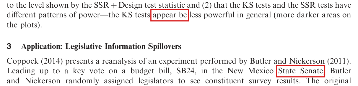
Three lines that end Section 2.2, the heading '3 Application: Legislative Information Spillovers', and three lines of Section 3. Red boxes mark the words 'appear be' in 'the KS tests appear be less powerful in general' and the words 'State Senate,' in 'in the New Mexico State Senate, Butler and Nickerson randomly assigned legislators'.
End of Section 2.2 and beginning of Section 3, p. 400. The marks show the misprint “appear be” and the chamber printed as “State Senate”.
Five lines of the reference list on page 402. In the entry that begins 'Brady, Henry E. 2008.', a red box marks the name 'Collier David,' in the list of editors 'Janet M. Box-Steffensmeier, Henry E. Brady and Collier David'.
Reference list, p. 402, the entry Brady (2008). The mark shows the editor’s name printed as “Collier David”.
Five lines of the reference list on page 403. A red box marks 'Hollander, Myles. 1999.' at the start of the entry 'Hollander, Myles. 1999. Nonparametric statistical methods, 2nd ed. Hoboken, NJ: Wiley-Interscience.'.
Reference list, p. 403. The mark shows the entry for the 1999 second edition of Nonparametric statistical methods, printed under one author.
Five lines of text from page 399. A red box marks the word 'controlgroups.' in 'a shift in the location of the distributions of the treated versus the controlgroups.'.
Second paragraph of p. 399. The mark shows the misprint “controlgroups”.
Six lines of the abstract on page 395. A red box, in two parts across a line break, marks the citation '(Hollander 1999, section 5.4)' after the words 'the simple Kolmogorov-Smirnov test statistic'.
Abstract, p. 395. The mark shows the citation of the 1999 book under one author.

The first mean in the comparison is the mean of y~i,Zi=0\tilde y_{i,Z_i=0} among the treated units, and its subscript is Zi=0Z_i=0, not Zi=1Z_i=1.

Section 2, first paragraph, p. 397 (PDF p. 3)

See also under Formal statements (Lean): P016-T17

As printed

For example, the implication of the constant, additive effects model, y~i,Zi=0=Yi−Ziτ\tilde y_{i,Z_i=0}=Y_i-Z_i\tau, only changes the distribution of outcomes for units in the treated condition. Comparing the mean of y~i,Zi=1∣Zi=1\tilde y_{i,\colorbox{#ffe58a}{$Z_i=1$}}|Z_i=1 to the mean of y~i,Zi=0∣Zi=0\tilde y_{i,Z_i=0}|Z_i=0 makes intuitive sense in this case

The problem

The comparison meant is between the mean of the adjusted outcome y~i,Zi=0\tilde y_{i,Z_i=0} in the treated group and its mean in the control group. The first term carries the subscript Zi=1Z_i=1. The quantity y~i,Zi=1\tilde y_{i,Z_i=1} is not defined in the note: the preceding sentence and p. 396 define only y~i,Zi=0\tilde y_{i,Z_i=0}. The conditioning event Zi=1Z_i=1 identifies the treated group correctly.

Evidence a derivation

The evidence is a derivation with a numerical illustration, and a check of the page. Let ui=Yi−Ziτu_i=Y_i-Z_i\tau. The comparison meant is mean⁡(u∣Z=1)−mean⁡(u∣Z=0)\operatorname{mean}(u\mid Z=1)-\operatorname{mean}(u\mid Z=0). If y~i,Zi=1\tilde y_{i,Z_i=1} is read as the treated potential outcome implied by the hypothesis, then it equals ui+τu_i+\tau, and the printed comparison equals mean⁡(u∣Z=1)−mean⁡(u∣Z=0)+τ\operatorname{mean}(u\mid Z=1)-\operatorname{mean}(u\mid Z=0)+\tau, which retains the hypothesized effect. With u=(0,1,2,3)u=(0,1,2,3), τ=10\tau=10 and Z=(0,0,1,1)Z=(0,0,1,1), the corrected comparison is 22 and the comparison under this literal reading is 1212. The replication code uses the same adjusted outcome for both groups.

What survives

The comparison meant, the randomization procedure and the inspected replication code are unchanged. I found no reported result that depends on this subscript.

Corrected

For example, the implication of the constant, additive effects model, y~i,Zi=0=Yi−Ziτ\tilde y_{i,Z_i=0}=Y_i-Z_i\tau, only changes the distribution of outcomes for units in the treated condition. Comparing the mean of y~i,Zi=0∣Zi=1\tilde y_{i,\colorbox{#ffe58a}{$Z_i=0$}}|Z_i=1 to the mean of y~i,Zi=0∣Zi=0\tilde y_{i,Z_i=0}|Z_i=0 makes intuitive sense in this case

Five lines of text from page 397. A red box marks the subscript Z_i=1 of the first y-tilde in the words 'Comparing the mean of y-tilde_i,Zi=1 given Z_i = 1 to the mean of y-tilde_i,Zi=0 given Z_i = 0'.
Section 2, first paragraph, p. 397. The mark shows the subscript Zi=1Z_i=1 of the first adjusted outcome in the comparison of means.

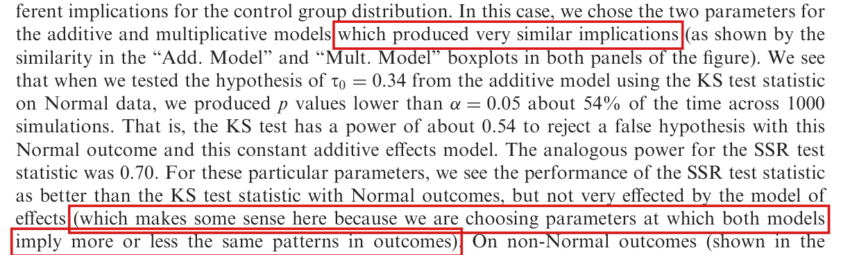
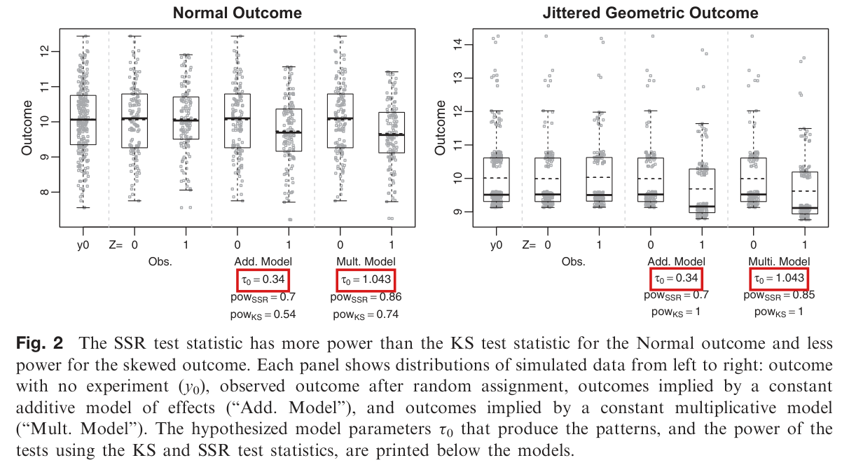
The additive and multiplicative hypotheses of Fig. 2 are not matched in strength: the replication code chooses the multiplicative parameter by a criterion that can match a single treated unit, and τ0=1.043\tau_0=1.043 implies an expected shift in the treated mean about 20% larger than τ0=0.34\tau_0=0.34 does.

Last paragraph of p. 398 (PDF p. 4), with the labels of Fig. 2 on the same page; the calibration is in the script ksvsssr-setup.R of the replication files, lines 52–61

See also under Formal statements (Lean): P016-T18, P016-T19

As printed

In this case, we chose the two parameters for the additive and multiplicative models which produced very similar implications (as shown by the similarity in the “Add. Model” and “Mult. Model” boxplots in both panels of the figure).

For these particular parameters, we see the performance of the SSR test statistic as better than the KS test statistic with Normal outcomes, but not very effected by the model of effects (which makes some sense here because we are choosing parameters at which both models imply more or less the same patterns in outcomes).

Fig. 2, Normal Outcome. Add. Model: τ0=0.34\tau_0=0.34, powSSR=0.7\mathrm{pow}_{\mathrm{SSR}}=0.7, powKS=0.54\mathrm{pow}_{\mathrm{KS}}=0.54. Mult. Model: τ0=1.043\tau_0=1.043, powSSR=0.86\mathrm{pow}_{\mathrm{SSR}}=0.86, powKS=0.74\mathrm{pow}_{\mathrm{KS}}=0.74.

Calibration in ksvsssr-setup.R, line 55: median(abs(mulres-addres)).

The problem

The text says that the two hypotheses of Fig. 2 were chosen to have very similar implications, and it uses this to explain why the comparison of SSR with KS is little affected by the model of effects. Read as a statement about the ordering of the two statistics, the text is correct: SSR has more power than KS for the Normal outcome and less for the skewed outcome under both hypotheses. The two hypotheses are not of equal strength, however, and the difference between the “Add.” and “Mult.” columns cannot be read as the effect of the model alone. The replication code chooses the multiplicative parameter by minimizing the median, over all 256 units, of the absolute difference between the outcomes that the two models generate under one assignment. Since the 128 control units contribute exact zeros, this median is half the smallest difference among the treated units, and it vanishes as soon as one treated unit matches. The parameter chosen, 1.04261.0426 (printed as 1.0431.043), lowers the expected adjusted treated mean of the Normal outcome by 0.4120.412. The additive hypothesis lowers it by 0.3430.343, and the multiplicative shift is about 20% larger.

Evidence an exact counterexample

The evidence is a derivation, an exact example, and a recalculation with the replication code.

For a no-effect outcome yiy_i and an assignment zz, the additive model with parameter tt generates yi+zity_i+z_it and the multiplicative model with parameter aa generates yi[1+zi(a−1)]y_i[1+z_i(a-1)]. The two agree for a control unit, and for a treated unit they differ by ∣(a−1)yi−t∣|(a-1)y_i-t|. With 128 control units and 128 treated units, the median of the 256 absolute differences is the average of the 128th and the 129th smallest, and the criterion equals

f(a)=12min⁡i:zi=1∣(a−1)yi−t∣.f(a)=\frac12\min_{i:z_i=1}|(a-1)y_i-t|.

For every treated unit jj such that yj≠0y_j\ne0, I have f(aj)=0f(a_j)=0 at the value aj=1+t/yja_j=1+t/y_j, whatever the differences for the other 127 treated units. The criterion can therefore match one treated unit without matching the group means.

For the exact example, let the control outcomes be 64 values equal to 99 and 64 equal to 1111, and let the treated outcomes be one 88, 63 nines, 63 elevens and one 1212, so that both groups have mean 1010. With t=34/99t=34/99 and a=1+t/8=413/396a=1+t/8=413/396 the criterion is exactly zero. The multiplicative adjustment then lowers the treated mean by 10(1−1/a)=170/41310(1-1/a)=170/413, which is 495/413≈1.20495/413\approx1.20 times tt.

For the recalculation, the data generation and the optimizer call of the replication code were run with the random number convention that R used in 2016. I find t=0.343434t=0.343434 at the grid entry used for Fig. 2 and a=1.042615a=1.042615, which round to the printed 0.340.34 and 1.0431.043. The mean of the Normal outcome is yˉ=10.069155\bar y=10.069155. Under complete randomization the expected treated mean is yˉ\bar y. The additive adjustment lowers the treated mean by tt under every assignment, and the multiplicative adjustment lowers it by (1−1/a)yˉ(1-1/a)\bar y in expectation.

Expected fall in the adjusted treated mean of the Normal outcome under the two hypotheses of Fig. 2, from the recalculation.
Multiplicative parameter aaMultiplicative, (1−1/a)yˉ(1-1/a)\bar yAdditive, ttExcess
1.0431.043, as printed0.41510.41510.34340.343420.9%20.9\%
1.0426151.042615, recalculated0.41160.41160.34340.343419.8%19.8\%

I did not simulate power at matched expected mean shifts. I have not shown that the larger shift accounts for the whole difference in power between the two columns, since the multiplicative adjustment also rescales the spread of the treated outcomes by 1/a1/a.

What survives

The printed powers stand as reports of the simulations that were run, and the ordering of SSR and KS within each column of Fig. 2 stands. Fig. 1, the network simulation of Fig. 3, which uses a separate grid, and the application do not use this calibration. A reading of the two columns as hypotheses of equal strength does not stand, and neither does the inference that the model of effects matters little at matched strength.

Corrected

In this case, the two parameters for the additive and multiplicative models were chosen by a criterion that can match the outcomes implied by the two models for one treated unit. The two hypotheses do not match the expected shift in the treated mean, which is about 0.340.34 under the additive hypothesis and about 0.410.41 under the multiplicative hypothesis.

SSR has greater power than KS for the Normal outcome under both hypotheses (0.700.70 versus 0.540.54 and 0.860.86 versus 0.740.74), and less power for the Jittered Geometric outcome. These comparisons preserve the ordering of the two statistics, but the hypotheses do not match the expected adjusted mean shifts.

For a comparison at matched expected mean shift, the multiplicative parameter is a=yˉ/(yˉ−t)a=\bar y/(\bar y-t), which is about 1.03531.0353 for t=0.3434t=0.3434 and yˉ=10.0692\bar y=10.0692, and the powers under that hypothesis must be computed anew. A calibration criterion should summarize the differences among the treated units only, not the median over the 128 unchanged control units and the 128 treated units.

Eleven lines of text from the last paragraph of page 398. Red boxes mark the words 'which produced very similar implications' and the parenthesis '(which makes some sense here because we are choosing parameters at which both models imply more or less the same patterns in outcomes).'.
Last paragraph of p. 398. The marks show the qualitative comparison of the two hypotheses, which does not establish equal expected mean shifts; the defect is in the calibration code.
Figure 2 of the note: two panels of boxplots, titled 'Normal Outcome' and 'Jittered Geometric Outcome', each with columns y0, Obs., Add. Model and Mult. Model, above the caption. Below the model columns are printed the parameters and powers: for the Normal outcome, tau_0 = 0.34 with pow_SSR = 0.7 and pow_KS = 0.54, and tau_0 = 1.043 with pow_SSR = 0.86 and pow_KS = 0.74; for the Jittered Geometric outcome, tau_0 = 0.34 with pow_SSR = 0.7 and pow_KS = 1, and tau_0 = 1.043 with pow_SSR = 0.85 and pow_KS = 1. Red boxes mark the four labels 'tau_0 = 0.34' and 'tau_0 = 1.043'.
Fig. 2 and its caption, p. 398. The marks show the hypothesized parameters printed below the “Add. Model” and “Mult. Model” boxplots of each panel: τ0=0.34\tau_0=0.34 and τ0=1.043\tau_0=1.043.

Formal statements (Lean)

Formal results: 17 whole; 3 restricted; 0 refuted; 1 omitted.

Coverage concerns the identified claim under its stated assumptions. A checked proof establishes the formal statement; correspondence to the published text was reviewed by AI. Repository access is currently required to open the source links.

Each result links to its current formal statement and proof. “Whole” covers the identified claim under its assumptions; “restricted” covers the stated narrower scope; “refuted” gives a counterexample to the identified assertion; “omitted” has no current theorem. Any named published theorem used as a premise remains an assumption. Browse the formal results for this work.

Section 2, the two sentences that lead into equation (1): the KS test ‘ignoring information about the joint distribution’ and the simplest SSR ‘including the correlation between treated and control outcomes as a part of the distribution of the statistic’, as printed; the witnesses are the validator's constructions and are not in the paper

p. 397 (PDF p. 3), Section 2, second paragraph, with equation (1)

p. 397 (PDF p. 3), Section 2, before equation (1). The pairing and assignment-design witnesses give both statistic tables, both tail masses and both design covariances.

Historical component credits
  • Counterexample proved AronowAudit.P016.t1_pairing_witness Historical support retained; baseline fidelity: ok; manifest: used; used in Solution; This is the target’s explicitly illustrative external pairing witness, not an assertion that the paper posits a pairing.
  • Counterexample proved AronowAudit.P016.t1_design_tables Historical support retained; baseline fidelity: ok; manifest: used; used in Solution; The assignment lists enumerate the specified supports without repetitions; zero-based indexing preserves their stated order.
  • Counterexample proved AronowAudit.P016.t1_design_probabilities Historical support retained; baseline fidelity: ok; manifest: used; used in Solution; Exact finite witness for T1(ii); the two covariance notions in T1 are kept distinct.

Section 2, the information contrast before equation (1), as repaired by Sol: the simple SSR is a function of the two group margins and its lower-tail test is the absolute difference-in-means test

p. 397 (PDF p. 3), Section 2, second paragraph, with equation (1)

p. 397 (PDF p. 3), Section 2, before equation (1), corrected claim. The simple SSR has the least-squares, moment, ordering, margin and design identities, with the network-alignment and scalar-KS witnesses.

Historical component credits
  • Proved AronowAudit.P016.t2_scalar_ks_witness Historical support retained; baseline fidelity: ok; manifest: used; used in Solution; This is a positive exact witness in corrected target T2(G), and also shows why equality of the scalar KS statistic is weaker than equality of both empirical margins.
  • Proved AronowAudit.P016.t2_least_squares Historical support retained; baseline fidelity: ok; manifest: used; used in Solution; The infimum has a nonempty range bounded below by zero, and the exported equality and coefficient equivalence identify the attained unique minimum.
  • Proved AronowAudit.P016.t2_decomposition Historical support retained; baseline fidelity: ok; manifest: used; used in Solution; The hypothesis n≥2 is redundant under the two positive group-size assumptions, and the claim itself includes all three.
  • Proved AronowAudit.P016.t2_tail_equivalence Historical support retained; baseline fidelity: ok; manifest: used; used in Solution; Fixed outcomes and fixed group sizes are explicit claim hypotheses, not added restrictions.
  • Proved AronowAudit.P016.t2_tail_probability Historical support retained; baseline fidelity: ok; manifest: used; used in Solution; The assignment-map formulation covers every finite target design, and the inclusive tails match. The public description states exactly these restrictions and this equality.
  • Proved AronowAudit.P016.t2_group_moments Historical support retained; baseline fidelity: ok; manifest: used; used in Solution; The group second moments use divisor n_g, exactly as the target formula requires.
  • Proved AronowAudit.P016.t2_rss_margin_invariance Historical support retained; baseline fidelity: ok; manifest: used; used in Solution; Redundant: the used t2_margin_invariance already gives both SSR and KS equality.
  • Proved AronowAudit.P016.t2_margin_invariance Historical support retained; baseline fidelity: ok; manifest: used; used in Solution; Equal multiset cardinalities imply nonempty groups for the second assignment; ties and multiplicities are retained. The public description accurately states this invariance theorem.
  • Proved AronowAudit.P016.t2_design_dependence Historical support retained; baseline fidelity: ok; manifest: used; used in Solution; An arbitrary finite probability space with an assignment map represents every target design by its pushforward; nonuniform and zero weights are allowed.
  • Proved AronowAudit.P016.t2_network_alignment Historical support retained; baseline fidelity: ok; manifest: used; used in Solution; The graph column is degree only, precisely the SSR + Degree witness in T2(F).

Section 3, the application model y0=yz−β1z−β2g(Γz)\mathbf{y}_0 = \mathbf{y}_{\mathbf{z}} - \beta_1\mathbf{z} - \beta_2 g(\Gamma\mathbf{z}) with ‘gg ... normalizes the sums of distances to treated neighbors to have unit variance’, and the rejection rule ‘pp values ... less than .05’ of Section 2.2, as printed; the witnesses are the validators' constructions and are not in the paper

p. 400 (PDF p. 6), Section 3, the unnumbered display and the two sentences after it; p. 400, Section 2.2, and the caption of Fig. 3, p. 401 (PDF p. 7), for the rejection rule

p. 400 (PDF p. 6), Section 3 and Section 2.2; Fig. 3, p. 401 (PDF p. 7). The four-unit, six-unit, recorded-table and cutoff witnesses establish the stated affine obstructions, regression minima and rejection-rule discrepancies.

Historical component credits
  • Counterexample proved AronowAudit.P016.t3_four_unit_exposure Historical support retained; baseline fidelity: ok; manifest: used; used in Solution; The row establishes the assigned affine-normalization witness; it makes no full refutation claim for an arbitrary unspecified vector-valued g.
  • Counterexample proved AronowAudit.P016.t3_determinants Historical support retained; baseline fidelity: ok; manifest: used; used in Solution; The target itself requires reading the displayed decimals as exact rationals; this is a direct match, so I retain faithful rather than the record’s faithful_with_notes classification.
  • Counterexample proved AronowAudit.P016.t3_table_not_affine Historical support retained; baseline fidelity: ok; manifest: used; used in Solution; The target is explicitly about the recorded rational rows, so no unavailable full-precision score reconstruction is required.
  • Counterexample proved AronowAudit.P016.t3_cutoff_witness Historical support retained; baseline fidelity: ok; manifest: used; used in Solution; The row is a numerical witness for the explicitly specified tail rules, not a claim about a particular simulated SSR dataset or general test validity.
  • Counterexample proved AronowAudit.P016.t3_six_unit_exposure Historical support retained; baseline fidelity: ok; manifest: used; used in Solution; All least-squares minima are exported as values of the actual infimum definition, rather than merely values at chosen coefficients.

Section 3, the application model and the description of the tests, as repaired by Sol: the centred similarity exposure, the application regression, and the two pp-value rules

p. 400 (PDF p. 6), Section 3, the unnumbered display and the two sentences after it; p. 400, Section 2.2, p. 398 (PDF p. 4) and the caption of Fig. 3, p. 401 (PDF p. 7), for the rejection rule

p. 400 (PDF p. 6), Sections 2.2 and 3; pp. 398 and 401, corrected claim. The bank-centered model has the stated cancellation, standardization, regression invariance, orientation, nonaffine witnesses and inclusive-tail cutoff identities.

Historical component credits
  • Proved AronowAudit.P016.t4_application_mapping Historical support retained; baseline fidelity: ok; manifest: used; used in Solution; The empty-design specialization is harmless: the row covers every nonempty target design as well. The forward-model premise is precisely T4(a), rather than an imported assumption of a substantive result.
  • Proved AronowAudit.P016.t4_cutoff_difference Historical support retained; baseline fidelity: ok; manifest: used; used in Solution; The general real-order identity specializes directly to the target p2 and loses no cases.
  • Proved AronowAudit.P016.t4_tail_coverage Historical support retained; baseline fidelity: ok; manifest: used; used in Solution; B>0 is the implicit requirement for the target proportions and is satisfied by the stated application and simulation sample sizes. There is no sampled-test calibration conclusion in this row.
  • Proved AronowAudit.P016.t4_standardization Historical support retained; baseline fidelity: ok; manifest: used; used in Solution; The infimum formulation has its ordinary meaning: the finite least-squares objective range is nonempty and nonnegative, and a finite-dimensional least-squares minimum is attained. No rank hypothesis is added.
  • Proved AronowAudit.P016.t4_centering_not_rescaling Historical support retained; baseline fidelity: ok; manifest: used; used in Solution; This is an explicit witness for need-not-be-affine, not a universal assertion that centering always changes the span.
  • Proved AronowAudit.P016.t4_similarity_orientation Limited support; baseline fidelity: narrower; manifest: used; used in Solution; {'source': 'adjudication+second review', 'adjudicator': 'P016/P016_Interference.lean:1645 places hm, requiring every bank assignment to have m treated units, before the entire three-part conclusion. T4(c) asserts the raw identity (Sz)_i = m - z_i - (Dz)_i/2 whenever the current z has m treated units, and introduces the fixed-size-bank condition only for the centered and standardized identities. A bank containing the all-control and all-treated assignments meets the standing coverage condition but fails hm for a mixed z, so this nontrivial case of the raw identity is excluded. The centered and standardized conclusions otherwise match their claimed scope.', 'suggested_fix': 'Move hm into an implication governing only the centered and standardized conclusions, leaving the raw-sum identity outside that implication; alternatively split off and credit a raw-identity declaration with no fixed-count-bank premise.', 'second_review': 'P016/P016_Interference.lean:1645 places the fixed-count-bank hypothesis hm at line 1648 before all three conclusions, including the raw similarity-sum identity. T4(c) requires that identity for every current assignment with m treated units and introduces the bank condition only for the centered and standardized identities. A bank containing the all-control and all-treated assignments satisfies coverage but fails hm for a mixed current assignment, excluding an allowed class of instances of the raw identity. Export the raw identity separately without hm, or move hm into an implication governing the final two conclusions.', 'severity': 'major'}

Section 2, the comparison of the information used by the KS and by the simplest SSR statistic, with equation (1); as printed

p. 397 (PDF p. 3), Section 2, second paragraph, and equation (1)

No current theorem is supplied for this target.

Historical component credits
  • Counterexample proved AronowAudit.P016.t5_printed_contrast_refuted Withdrawn support; baseline fidelity: wrong_credit; manifest: not used; Solution use unverified; Marked wrong_credit: fixed empirical-margin invariance does not refute the printed distribution-level information comparison.

Section 3, the application model, and the rejection rule of the simulations; as printed

p. 400 (PDF p. 6), Section 3, the unnumbered display and the sentences around it; p. 400, Section 2.2; caption of Fig. 3, p. 401 (PDF p. 7); p. 398 (PDF p. 4)

p. 400 (PDF p. 6), Section 3 and Section 2.2; pp. 398 and 401, as printed. For any map g with across-unit sample variance one on every assignment of a nonempty finite design, the displayed generation equation implies recovery of the baseline outcomes; the printed rejection convention is p < 1/20.

Historical component credits
  • Proved AronowAudit.P016.t6_printed_model_consistency Limited support; baseline fidelity: narrower; manifest: not used; not used in Solution; The used general finite-design theorem contains this single-assignment cancellation, with the same sample-variance restriction.
  • Proved AronowAudit.P016.t6_printed_cutoff Historical support retained; baseline fidelity: ok; manifest: used; used in Solution; {'source': 'adjudication', 'decision': 'rejected', 'what': "P016/P016_Interference.lean:659 states printedReject p iff p < 1/20, with printedReject defined at line 539 by precisely that strict inequality. T6's component here is the printed rejection convention, expressed as p values less than .05, and 1/20 is exactly .05. A definitional transcription supplies all the content claimed for this component; the row promises neither a size bound nor verification of the released implementation. Its definitional proof therefore creates no fidelity defect."}
  • Proved AronowAudit.P016.t6_printed_general_model_consistency Limited support; baseline fidelity: narrower; manifest: used; used in Solution; {'source': 'adjudication+second review', 'adjudicator': 'P016/P016_Interference.lean:667 requires sampleVariance(g(Γz)) = 1 on every design assignment through hg at line 670; sampleVariance fixes divisor n-1 at line 505. Printed T6 only requires g to normalize exposure to unit variance and does not restrict it to this divisor. For two units with Γ = [[0,1],[1,0]] and the two one-treated assignments, population standardization gives vectors (-1,1) and (1,-1), whose population variance is one but sample variance is two. These nondegenerate normalizers are excluded, although the same model-consistency cancellation holds at the original g and coefficient values.', 'suggested_fix': 'Remove hg from the credited consistency theorem while retaining the displayed-model premise hy, so consistency holds for every g. Normalization can be specified separately without restricting this algebraic result to the n-1 convention.', 'second_review': "P016/P016_Interference.lean:667 requires sampleVariance(g(Gamma z)) = 1 throughout the design at line 670, with divisor n-1 fixed at line 505. T6's printed claim describes g as normalizing to unit variance without specifying that divisor, so it also permits population normalization. For two units with off-diagonal distances one and the two one-treated assignments, population normalization yields (-1,1) and (1,-1), each of population variance one but sample variance two, excluding nondegenerate model instances at their given parameters. Remove hg from the consistency statement and retain the model premise hy; the cancellation applies to arbitrary g.", 'severity': 'major'}

Section 1, step (4) of the testing procedure, ‘comparing the observed test statistic, T(Yi,Zi)\mathcal{T}(Y_i, Z_i) against the distribution of that test statistic that characterizes the hypothesis’, as printed; the witnesses are the validator's constructions and are not in the paper

p. 396 (PDF p. 2), Section 1, second full paragraph, steps (2)–(4)

p. 396 (PDF p. 2), Section 1, steps (2)-(4). The four-unit mean and seventy-assignment KS witnesses show probability-one rejection of true additive hypotheses by the literal raw-versus-adjusted comparison, with the stated corrected reference probabilities.

Historical component credits
  • Counterexample proved AronowAudit.P016.t7_mean_witness Historical support retained; baseline fidelity: ok; manifest: used; used in Solution; The row is the numerical witness component of T7(i); the separate credited row R114-11 exports rejection with probability one for every positive level.
  • Counterexample proved AronowAudit.P016.t7_mean_rejects_truth Historical support retained; baseline fidelity: ok; manifest: used; used in Solution; This witnesses the literal raw-argument recipe using the target absolute-tail convention; it does not refute the intended adjusted procedure or every possible choice of tail.
  • Proved AronowAudit.P016.Wave1.t7_ks_witness_proof Historical support retained; baseline fidelity: ok; manifest: used; used in Solution; The target specifies inclusive upper tails and a strict .05 cutoff for this witness. The paper itself gives no tail formula; this is the stated literal-argument witness, not a claim that every interpretation of the printed comparison is invalid. Metadata status proved and resolution theorem_proved refer to a proved witness theorem and do not conflict with target_kind counterexample.

Section 1, step (4) of the testing procedure, corrected: the observed statistic is T(y~i,Zi=0,Zi)\mathcal{T}(\tilde y_{i,Z_i=0}, Z_i) at the realized assignment

p. 396 (PDF p. 2), Section 1, second full paragraph, step (4)

p. 396 (PDF p. 2), Section 1, step (4), corrected claim. The additive adjustment fixes the true baseline, gives the same observed and reference law with calibrated inclusive upper tails, and removes exactly the raw mean shift.

Historical component credits
  • Proved AronowAudit.P016.t8_additive_mapping Historical support retained; baseline fidelity: ok; manifest: used; used in Solution; Both identities apply to arbitrary finite baselines and additive parameters, exactly as required by T8(a).
  • Proved AronowAudit.P016.t8_corrected_comparison Historical support retained; baseline fidelity: ok; manifest: used; used in Solution; {'source': 'adjudication', 'decision': 'rejected', 'what': 'P016_Interference.lean:1780 gives both the equality of statistic laws and the inclusive upper-tail bound for every alpha in [0,1], as required by T8(b). By the definitions at lines 84 and 88, true additive generation followed by adjustment returns y0 for every assignment, so the observed-assignment index in the inner reference expression does not make the adjusted vector vary across reference draws. Every target assignment design is recovered by taking its finite assignment subtype as Omega and the inclusion as assign; allowing duplicate indices, zero weights, or index-sensitive statistics excludes no target case. Finite support also makes arbitrary event predicates harmless.'}
  • Proved AronowAudit.P016.t8_raw_mean_shift Historical support retained; baseline fidelity: ok; manifest: used; used in Solution; The control-nonempty hypothesis is included in the target even though only treated positivity is needed for this shift identity.

The three displayed definitions of the test statistics as printed: the KS formula of footnote 3 (no absolute value), equation (1) (mean not specified) and equation (2) (no row index; no intercept listed); the witnesses are the validator's constructions and are not in the paper

footnote 3, p. 396 (PDF p. 2); equation (1), p. 397 (PDF p. 3); equation (2) and the sentence before it, p. 399 (PDF p. 5)

footnote 3, p. 396; equation (1), p. 397; equation (2), p. 399. The signed-KS, pooled-mean and missing-intercept readings give the three specified discrepancies, including the general constant-statistic law and inclusive tails and the complete six-assignment SSR table.

Historical component credits
  • Counterexample proved AronowAudit.P016.t9_signed_ks_witness Historical support retained; baseline fidelity: ok; manifest: used; used in Solution; The signed statistic is a legitimate one-sided maximum. The target component is its discrepancy from the described two-sided statistic, rather than invalidity of one-sided KS testing.
  • Counterexample proved AronowAudit.P016.t9_pooled_witness Historical support retained; baseline fidelity: ok; manifest: used; used in Solution; The row is a discrepancy witness under the pooled interpretation, not a universal formal theorem about every u and every design. The target note expressly identifies the pooled interpretation as conditional on a meaning of the undefined bar.
  • Counterexample proved AronowAudit.P016.t9_intercept_witness Historical support retained; baseline fidelity: ok; manifest: used; used in Solution; The intended component is the discrepancy witness under the explicitly listed-regressors-only interpretation. As the target note warns, this does not establish that an unstated intercept is itself a paper error.

Footnote 3 and equations (1) and (2), corrected: the two-sided KS distance, the group-mean residual sum of squares and the indexed least-squares residual sum of squares with an intercept

footnote 3, p. 396 (PDF p. 2); equation (1), p. 397 (PDF p. 3); equation (2) and the sentence before it, p. 399 (PDF p. 5)

footnote 3, p. 396; equation (1), p. 397; equation (2), p. 399, corrected claim. The corrected SSR minima are attained with unique fitted values, KS equals its threshold supremum and is label invariant in [0,1], and symmetric adjacency gives the stated network columns.

Historical component credits
  • Proved AronowAudit.P016.t10_general_least_squares Historical support retained; baseline fidelity: ok; manifest: used; used in Solution; Attainment and uniqueness of the fitted vector hold for every real design matrix on exactly the nonempty-group outcome domain of T10(b).
  • Proved AronowAudit.P016.t10_ks_supremum Historical support retained; baseline fidelity: ok; manifest: used; used in Solution; The sample KS maximum is equated with the threshold supremum, with label symmetry and the full [0,1] range as required by T10(c).
  • Proved AronowAudit.P016.Wave1.t10_symmetric_network Historical support retained; baseline fidelity: ok; manifest: used; used in Solution; The symmetric binary-network identities retain diagonal entries and exactly establish T10(d) on the stated nonempty-group domain.
  • Proved AronowAudit.P016.t2_least_squares Historical support retained; baseline fidelity: ok; manifest: used; used in Solution; The statement establishes the group-centered minimum and unique intercept/slope coefficients of T10(a), with only the redundant n≥2 premise.

Section 1, ‘test statistics with this property (“effect increasing” test statistics)’, which identifies a statistic that is small for similar and large for divergent distributions with an effect increasing statistic, as printed; the witnesses are the validator's constructions and are not in the paper

pp. 396–397 (PDF pp. 2–3): the quotation that runs from the last line of p. 396 to the first lines of p. 397, and the sentence after it

pp. 396-397 (PDF pp. 2-3), the quoted statistic criterion and following sentence. The weak and strict KS witnesses and the two opposite SSR changes refute effect-increasing monotonicity for both KS versions and both SSR orientations.

Historical component credits
  • Counterexample proved AronowAudit.P016.t11_ks_witness Historical support retained; baseline fidelity: ok; manifest: used; used in Solution; The actual vectors meet the directional effect-increasing antecedent; no definition of effect increasing is assumed as a premise. This says nothing about bias or validity of randomization p values.
  • Counterexample proved AronowAudit.P016.t11_rss_witness Historical support retained; baseline fidelity: ok; manifest: used; used in Solution; The explicit unchanged control coordinates supply the required control direction even though the exported coordinatewise inequalities alone do not express the general effect-increasing antecedent. The target note says the paper does not claim SSR is effect increasing; this is an auxiliary validator witness, as credited.

Section 1, the two sentences after the quotation of BFP's advice, as repaired by Sol: the effect increasing property stated, and sharp-null validity for any test statistic

p. 397 (PDF p. 3), first paragraph, second and third sentences

p. 397 (PDF p. 3), first paragraph, second and third sentences. The mean contrast is effect increasing on nonempty groups, whereas both KS statistics fail this directional condition. Every statistic calibrated under a positive finite assignment law has valid inclusive upper, lower, and doubled minimum tails, at weak and strict cutoffs. For the uniform two-of-four design and outcomes (0,1,2,3), the KS scores are (1,1/2,1/2,1/2,1/2,1), the upper p values are (1/3,1,1,1,1,1/3), and the rejection probabilities are 0, 1/3, and 1 on the stated threshold ranges.

Historical component credits
  • Proved AronowAudit.P016.t12_upper_valid Historical support retained; baseline fidelity: ok; manifest: used; used in Solution; The inclusive upper-tail calibration bound matches the upper-tail component of T12(iii).
  • Proved AronowAudit.P016.t12_lower_valid Historical support retained; baseline fidelity: ok; manifest: used; used in Solution; The inclusive lower-tail bound uses the strictly positive finite law and [0,1] level domain explicitly required by T12(iii).
  • Proved AronowAudit.P016.t12_two_tail_valid Historical support retained; baseline fidelity: ok; manifest: used; used in Solution; The inclusive capped doubled-minimum calibration bound matches the two-tail component of T12(iii).
  • Proved AronowAudit.P016.t12_ks_p_table Historical support retained; baseline fidelity: ok; manifest: used; used in Solution; The six exact upper p-values equal the table required by the fixed example in T12(iv).
  • Proved AronowAudit.P016.t12_ks_size Historical support retained; baseline fidelity: ok; manifest: used; used in Solution; The exact rejection probability has precisely the three threshold ranges specified in T12(iv).
  • Proved AronowAudit.P016.t12_mean_effect_increasing Historical support retained; baseline fidelity: ok; manifest: used; used in Solution; The definition expands to the directional mean-difference monotonicity on nonempty groups required by T12(i). The n<2 cases are empty-domain cases, but the universally quantified family has nondegenerate instances for every n≥2.
  • Proved AronowAudit.P016.t12_ks_not_effect_increasing Historical support retained; baseline fidelity: ok; manifest: not used; not used in Solution; Its conclusion uses the total extension of KS to empty groups. The solution instead instantiates its existing exported four-unit witness to state failure on nonempty groups.

The simulated permutation tests of Section 2.2 as the archived code implements them (raw empirical tail proportions; rejection when p≤.05p \le .05), set against ‘they reject the true null ... no more than 5% of the time at α=.05\alpha = .05’; the witnesses are the validator's constructions and are not in the paper

p. 400 (PDF p. 6), Section 2.2, first and second paragraphs; p. 397 (PDF p. 3), the parenthesis ‘(in that the test should produce pp values less than α\alpha no more than 100α%100\alpha\% of the time when the null is true)’; code: pkgs/RItools/R/zzpvalues.R, simulation/teststat-parallel-results.R

p. 400 (PDF p. 6), Section 2.2, and p. 397 (PDF p. 3), validity parenthesis; archived simulation weak-cutoff rule. Tie-free exchangeable scores have uniform ranks and raw weak-cutoff rejection probability 2(c+1)/(B+1) whenever c=floor(alpha B/2) and 2c<B. At .05 the sizes for B=1000 and 10000 exceed .05. In the uniform eight-of-sixteen design with fixed outcomes 2^i, the SSR has the stated moment formula and 6435 values, each on a complementary pair. Independent uniform observed and reference draws give the exact binomial-mixture rejection laws and bounds, including every positive B for the weak .05 rule. All five reported decimal prefixes are certified by open rational intervals. The strict .05 sizes are below .05, and raw p=0 has the stated positive power-sum probability. These witnesses concern the archived weak cutoff; they do not refute the printed strict rule.

Historical component credits
  • Proved AronowAudit.P016.t13_no_ties Limited support; baseline fidelity: narrower; manifest: used; used in Solution; {'source': 'adjudication+second review', 'adjudicator': "P016_Interference.lean:2365 correctly expresses the uniform rank law, the almost-sure count identities, and the weak-cutoff size formula of T13(i) under exchangeability and almost-sure distinctness. Its extra alpha < 1 hypothesis excludes the target's admissible alpha = 1 case when B is odd; then c = (B-1)/2, rawP <= 1 always, and 2(c+1)/(B+1) = 1. Nonnegative thresholds above 1 that still satisfy 2c < B give the same trivial identity. Thus the noted restriction is a literal but mathematically trivial narrowing; I partly confirm it as narrower_than_claim/minor under the stated exception, with no substantive failure of the rank calculation.", 'suggested_fix': 'Remove hα1 : alpha < 1 from t13_no_ties, retaining 0 <= alpha, c = Nat.floor (alpha*B/2), and 2*c < B; handle alpha >= 1 by the probability-one identity. All substantive cases and the .05 witnesses already match the target.', 'second_review': 'P016/P016_Interference.lean:2365 adds alpha < 1 at line 2367, whereas T13(i) requires the size formula whenever c = floor(alpha B/2) and 2c < B. At alpha = 1 with odd B, the target permits c = (B-1)/2, rawP is always at most one by its definition at line 1374, and both sides of the formula equal one. Thus the statement omits only a trivial boundary case within the usual level range; remove the strict upper-bound premise and handle that case separately.', 'severity': 'minor'}
  • Proved AronowAudit.P016.t13_rss_identity Historical support retained; baseline fidelity: ok; manifest: used; used in Solution; The finite-design declaration already includes the same moment and RSS identity on the balanced design used in this claim.
  • Proved AronowAudit.P016.t13_finite_design Historical support retained; baseline fidelity: ok; manifest: used; used in Solution; The fixed power-of-two population has exactly the balanced support, moments, RSS identity, image cardinality, and complementary-pair fibers required by T13(ii). This row is an auxiliary or mechanism component, not a standalone full refutation of a printed validity claim.
  • Proved AronowAudit.P016.Wave1.t13_finite_rejection_proof Historical support retained; baseline fidelity: ok; manifest: used; used in Solution; The exact independent finite-design mixture, weak and strict cutoff inequalities, and positive zero-p probability establish the finite witness components T13(ii)–(iii), with no assertion refuting the printed strict rule. This is a counterexample to the target’s explicitly specified archived weak-cutoff algorithm, not to the paper’s strict rejection rule or its reported simulation rates.
  • Proved AronowAudit.P016.t13_numeric_certificates Historical support retained; baseline fidelity: ok; manifest: used; used in Solution; The closed rational calculations are the advertised arithmetic auxiliaries for the no-ties size and finite-witness lower bound, without purporting to prove a probability law. This row is an auxiliary or mechanism component, not a standalone full refutation of a printed validity claim.

The level of the simulated permutation tests of Section 2.2, as repaired by Sol: the printed strict cutoff, and the rank-corrected Monte Carlo pp value

p. 400 (PDF p. 6), Section 2.2, first and second paragraphs; p. 397 (PDF p. 3), the parenthesis on validity

p. 400 (PDF p. 6), Section 2.2, and the validity parenthesis on p. 397 (PDF p. 3). Exchangeable references give rank bounds, the printed strict-cutoff guarantees, valid corrected tails, and iid permutation invariance. Exact-tail clause (e) uses the strictly positive finite-law domain of its explicit reference to canonical T12(iii); the iid exchangeability clause permits zero-weight points.

Historical component credits
  • Proved AronowAudit.P016.t14_rank_bound Historical support retained; baseline fidelity: ok; manifest: used; used in Solution; Natural c represents exactly the target integers 0≤c≤B. Both count comparisons are inclusive and ties are permitted.
  • Proved AronowAudit.P016.t14_strict_bound Historical support retained; baseline fidelity: ok; manifest: used; used in Solution; The rejection cutoff is strictly <α, while each reference count is inclusive. The declaration does not claim this ceiling expression is ≤α for all α; the .05 specializations are supplied by R116-06.
  • Proved AronowAudit.P016.t14_corrected_valid Historical support retained; baseline fidelity: ok; manifest: used; used in Solution; The Borel joint-law formulation loses no real random-variable law; permutation maps and rank events are measurable, and probability normalization makes μ.real an ordinary finite real probability. The public correction summary agrees with the target.
  • Proved AronowAudit.P016.t14_iid_exchangeable Historical support retained; baseline fidelity: ok; manifest: used; used in Solution; {'source': 'adjudication', 'decision': 'rejected', 'what': 'P016_Interference.lean:2726 asserts invariance of every event probability under every permutation of the B+1 statistic coordinates. The iidMass and iidWeight definitions at lines 2698 and 2713 use the product of one normalized finite law, so this is exactly exchangeability in T14(d). Standing assumption S9 makes assignment designs finite, and any fixed outcome vector is absorbed by s(z) = T(y,z), so neither the finite representation nor the scalar statistic adds a restriction. Allowing B = 0 merely extends the statement to a trivial one-coordinate case.'}
  • Proved AronowAudit.P016.t14_printed_bounds Historical support retained; baseline fidelity: ok; manifest: used; used in Solution; This row is accurately advertised as the arithmetic corollary, not as a separate probabilistic validity theorem.
  • Proved AronowAudit.P016.t12_upper_valid Limited support; baseline fidelity: narrower; manifest: used; used in Solution; {'source': 'adjudication+second review', 'adjudicator': "P016/P016_Interference.lean:297 requires hP, strict positivity at every point of Ω, while T14(e) asserts exact upper-tail validity without that ambient-domain restriction. Thus a normalized law represented with zero-weight points cannot be supplied directly to this declaration. Removing those points changes neither upperP at any positive-weight observation nor the rejection-event mass, so every excluded law reduces trivially to its positive support. The formal narrowing is real but minor, rather than the reviewer's major fidelity problem.", 'suggested_fix': 'Remove the unused hP premise, or reassign this T14(e) credit to upper_tail_bound at line 237, which already states the unrestricted exact upper-tail bound.', 'second_review': "P016/P016_Interference.lean:297 adds hP, strict positivity at every point, although T14(e)'s exact inclusive upper-tail validity does not impose it. FiniteLaw at line 103 permits zero weights, whose removal leaves upperP at positive-weight observations and rejection-event mass unchanged under the definitions at lines 110 and 126. The omitted cases are therefore mathematically trivial; remove hP or credit the unrestricted upper_tail_bound at line 237.", 'severity': 'minor'}
  • Proved AronowAudit.P016.t12_lower_valid Limited support; baseline fidelity: narrower; manifest: used; used in Solution; {'source': 'adjudication+second review', 'adjudicator': "P016/P016_Interference.lean:305 adds hP, strict positivity at every point of Ω, whereas T14(e)'s exact lower-tail validity statement imposes no such condition on the ambient finite domain. FiniteLaw at line 103 permits zero weights, so the credited declaration is formally narrower when Ω is held fixed. However, zero-weight points contribute nothing to any tail or event probability: restriction to the positive support preserves lowerP at every possible observation and preserves the rejection probability. The omitted cases are therefore mathematically trivial, making this a minor scope defect rather than the flagged major problem.", 'suggested_fix': 'Remove the unused hP premise, as in the existing lower_tail_bound declaration at line 257, or reassign this overlapping T14(e) credit to that unrestricted declaration.', 'second_review': 'P016/P016_Interference.lean:305 requires every point to have strictly positive weight, while T14(e) requires exact inclusive lower-tail validity for the assignment distribution without that restriction. FiniteLaw at line 103 allows zero weights, and mass and lowerP at lines 110 and 130 show that deleting zero-weight points preserves tails at possible observations and the rejection probability. The restriction is therefore real but mathematically trivial; remove hP or credit the unrestricted lower_tail_bound at line 257.', 'severity': 'minor'}
  • Proved AronowAudit.P016.t12_two_tail_valid Limited support; baseline fidelity: narrower; manifest: used; used in Solution; {'source': 'adjudication+second review', 'adjudicator': "P016/P016_Interference.lean:313 requires strictly positive weight at every point of Ω, beyond the finite nonnegative normalized law allowed by T14(e)'s exact doubled-minimum validity claim. This is a formal restriction on laws represented on a fixed ambient domain, notwithstanding the row's reference to T12(iii). Its only excluded cases have zero-weight points, whose removal preserves both inclusive tails at positive-weight observations, their capped doubled minimum, and the probability of rejection. Consequently the narrowing is minor under the exception for mathematically trivial excluded cases, rather than major.", 'suggested_fix': 'Remove the unused hP premise, or reassign this T14(e) credit to the unrestricted two_tail_bound declaration at line 267 with the same alpha assumptions.', 'second_review': "P016/P016_Interference.lean:313 requires strictly positive weight at every point, beyond T14(e)'s exact-law validity claim for the capped doubled minimum of inclusive tails. The definitions of mass, upperP, lowerP and doubledP at lines 110, 126, 130 and 134 imply that removing zero-weight points preserves the test's rejection probability. This is a minor statement restriction even though the description discloses it; remove hP or credit two_tail_bound at line 267, which already has the required scope.", 'severity': 'minor'}

Three local statements as printed: ‘the hypotheses only have different implications for the control group distribution’ (p. 398); the ECDF ‘records the proportion of the distribution of xx at or below xix_i’ (footnote 3); ‘we tested the hypothesis τ=τ0,β=τ0\tau = \tau_0, \beta = \tau_0’ (p. 400); the witnesses are the validator's constructions and are not in the paper

p. 398 (PDF p. 4), last paragraph; footnote 3, p. 396 (PDF p. 2); p. 400 (PDF p. 6), Section 2.2, first paragraph

p. 398 (PDF p. 4), last paragraph; footnote 3, p. 396 (PDF p. 2); and p. 400 (PDF p. 6), Section 2.2. The specified adjustment, ECDF, and diagonal-hypothesis witnesses establish all three local mathematical errors.

Historical component credits
  • Counterexample proved AronowAudit.P016.t15_adjustment_witness Historical support retained; baseline fidelity: ok; manifest: used; used in Solution; The two explicit adjusted vectors and treated ECDF values give the required T15(a) witness, with unchanged controls visible in the vector equalities. The displayed vector equalities explicitly preserve the two control coordinates; no missing separate control-ECDF theorem is needed for this witness.
  • Counterexample proved AronowAudit.P016.t15_ecdf_witness Historical support retained; baseline fidelity: ok; manifest: used; used in Solution; The ECDF values at 2 and 3 for sample (1,3) exactly give the T15(b) witness.
  • Counterexample proved AronowAudit.P016.t15_diagonal_witness Historical support retained; baseline fidelity: ok; manifest: used; used in Solution; The diagonal-family equivalence and exclusion of (1/2,2) are precisely T15(c).

The three local statements of p. 398, footnote 3 and p. 400, corrected: ‘treated group distribution’; ‘at or below xx’; ‘τ=τ0,β=β0\tau = \tau_0, \beta = \beta_0’

p. 398 (PDF p. 4), last paragraph; footnote 3, p. 396 (PDF p. 2); p. 400 (PDF p. 6), Section 2.2, first paragraph

p. 398 (PDF p. 4), last paragraph; footnote 3, p. 396 (PDF p. 2); p. 400 (PDF p. 6), Section 2.2, first paragraph. Under additive and nonzero multiplicative hypotheses, control outcomes and control empirical distributions stay fixed. Treated outcomes have the stated parameter dependence, with nonzero response for the multiplicative comparison. The sample ECDF counts observations at or below its argument. Empirical distributions are asserted on their nonempty-sample domains. The joint family with separate parameter indices contains the truth (1/2,2), which belongs to no member of the printed diagonal family.

Historical component credits
  • Proved AronowAudit.P016.t16_group_adjustments Historical support retained; baseline fidelity: ok; manifest: used; used in Solution; The nonzero observed response qualification in the multiplicative parameter-dependence assertion is explicitly present in both the corrected target and Lean.
  • Proved AronowAudit.P016.t16_control_ecdf Historical support retained; baseline fidelity: ok; manifest: used; used in Solution; {'source': 'adjudication', 'decision': 'rejected', 'what': "P016_Interference.lean:2941 states that both additive and multiplicative adjustments leave the control ECDF unchanged at every real threshold, exactly the empirical-distribution component of T16(a). The nonzero multiplicative parameter matches the target's domain and restricts no additive parameter, since t is independent and a can always be chosen as 1. With a nonempty control group the ecdf definition at line 64 is the ordinary empirical proportion; its value 0 for an empty group is only an additional total-division convention. The ordinary nonempty-group identity does not hold merely by that convention."}
  • Proved AronowAudit.P016.t16_ecdf_argument Historical support retained; baseline fidelity: ok; manifest: used; used in Solution; {'source': 'adjudication', 'decision': 'rejected', 'what': "P016_Interference.lean:2953 equates sampleECDF u x with the number of indices satisfying u i <= x divided by n, precisely T16(b)'s corrected explanation of the argument x. The definition at line 68 is the target's indicator-sum formula, so converting that sum to a cardinality expresses the intended mathematical identity. Total division at n = 0 extends the identity by 0 = 0, while every positive-size sample retains its usual proportion; this makes neither the whole statement vacuous nor the target domain narrower."}
  • Proved AronowAudit.P016.t16_joint_hypothesis Historical support retained; baseline fidelity: ok; manifest: used; used in Solution; The weak-looking existential is sufficient here because the target component is precisely membership of the fixed truth (1/2,2), together with its exclusion from the diagonal.

Section 2, first paragraph, ‘Comparing the mean of y~i,Zi=1∣Zi=1\tilde y_{i,Z_i=1}|Z_i = 1 to the mean of y~i,Zi=0∣Zi=0\tilde y_{i,Z_i=0}|Z_i = 0’, corrected: the first term is y~i,Zi=0∣Zi=1\tilde y_{i,Z_i=0}|Z_i = 1

p. 397 (PDF p. 3), Section 2, first paragraph

p. 397 (PDF p. 3), Section 2, first paragraph. The corrected comparison uses two adjusted group means, whereas the conditional imputed-treated reading gives the raw contrast, with the stated 2-versus-12 instance.

Historical component credits
  • Proved AronowAudit.P016.t17_adjusted_comparison Historical support retained; baseline fidelity: ok; manifest: used; used in Solution; The printed treated symbol is undefined; the target explicitly makes the u+t interpretation diagnostic and conditional. This row faithfully proves those conditional algebraic identities, not a full refutation of a well-defined printed assertion.
  • Proved AronowAudit.P016.t17_comparison_witness Historical support retained; baseline fidelity: ok; manifest: used; used in Solution; The target itself states this witness in terms of u,τ,Z, so no additional raw-outcome premise or probability law is owed by this row. It is an illustrative exact instance, not a refutation of the undefined printed symbol.

The choice of the multiplicative parameter of Fig. 2 (‘we chose the two parameters for the additive and multiplicative models which produced very similar implications’), read as a match of the strength of the two hypotheses; the witness is the validator's construction and is not in the paper

p. 398 (PDF p. 4), last paragraph, and the labels of Fig. 2 on the same page; p. 399 (PDF p. 5), first sentences; code: simulation/ksvsssr-setup.R, lines 52–61

p. 398 (PDF p. 4), last paragraph and Fig. 2; p. 399 (PDF p. 5), first sentences; released calibration code. The specified 256-unit witness attains the global minimum zero of the median criterion despite 127 unmatched treated units and unequal generated and adjusted mean shifts.

Historical component credits
  • Counterexample proved AronowAudit.P016.t18_calibration_witness Historical support retained; baseline fidelity: ok; manifest: used; used in Solution; The target explicitly asks for constructed data, population variance with divisor 256, and the ordinary even median; all match directly. Zero is a global lower bound for a median of absolute discrepancies for every parameter, so the stated zero median is a minimum without further population hypotheses; the record’s historical proof-status remarks were not used in this statement-only audit.

The comparison of the additive and multiplicative columns of Fig. 2, as repaired by Sol: the two hypotheses are not matched in expected mean shift; the calibration criterion and the matched parameter

p. 398 (PDF p. 4), last paragraph, and the labels of Fig. 2; p. 399 (PDF p. 5), first sentences

p. 398 (PDF p. 4), last paragraph and Fig. 2; p. 399 (PDF p. 5), first sentences. The median criterion sees only the least treated discrepancy, has the stated roots, and does not match mean reductions, whose unique matching parameter is identified.

Historical component credits
  • Proved AronowAudit.P016.t19_discrepancy_formula Historical support retained; baseline fidelity: ok; manifest: used; used in Solution; Positive m is implicit in the target median framework; for this coordinate identity the excluded m=0 case has no coordinate i and contributes no missing assertion. No change from the saved claim-stage verdict.
  • Proved AronowAudit.P016.t19_root_discrepancies Historical support retained; baseline fidelity: ok; manifest: used; used in Solution; This is the component discrepancy calculation in part (c); median zero and global minimality are separately exported by R117-02. No change from the saved claim-stage verdict.
  • Proved AronowAudit.P016.t19_median_nonneg Historical support retained; baseline fidelity: ok; manifest: not used; not used in Solution; The calibration-roots declaration already includes global nonnegativity for clause (c); this row is used separately to certify the minimum in T18.
  • Proved AronowAudit.P016.t19_median_identity Historical support retained; baseline fidelity: ok; manifest: used; used in Solution; The sorted median uses both middle order statistics with multiplicities; m>0 makes both accesses valid, and the infimum is an attained minimum. No change from the saved claim-stage verdict.
  • Proved AronowAudit.P016.t19_calibration_roots Historical support retained; baseline fidelity: ok; manifest: used; used in Solution; The outcome y_j≠0 is exactly the root construction requirement; there is no extra positivity condition on the multiplier, and the criterion is minimized over all real multipliers. No change from the saved claim-stage verdict.
  • Proved AronowAudit.P016.t19_mean_reductions Historical support retained; baseline fidelity: ok; manifest: used; used in Solution; This is an acceptable generalization: the target balanced identities follow by specialization. It is not a narrowing and does not change either adjustment formula. No change from the saved claim-stage verdict.
  • Proved AronowAudit.P016.t19_expected_reductions Historical support retained; baseline fidelity: ok; manifest: used; used in Solution; Fixing y across assignments expresses the no-effect schedule. UniformExpectation averages the full complete balanced design, and m>0 ensures nonempty groups and support. No change from the saved claim-stage verdict.
  • Proved AronowAudit.P016.t19_matched_parameter Historical support retained; baseline fidelity: ok; manifest: used; used in Solution; {'source': 'adjudication', 'decision': 'rejected', 'what': "P016_Interference.lean:3527 states (1-1/a)*mu = t iff a = mu/(mu-t), with exactly T19(e)'s hypotheses mu != 0 and mu != t. Abstracting the population mean to an arbitrary real scalar imposes no restriction, and the statement matches the expected adjusted mean reductions rather than forward model shifts. At the additional a = 0 case, Lean's total division makes the left side mu = t, which is false, and the right side is also false because mu/(mu-t) is nonzero. Thus the convention adds no false matching parameter and loses no meaningful case."}
  • Proved AronowAudit.P016.t19_mismatch_numbers Historical support retained; baseline fidelity: ok; manifest: used; used in Solution; This auxiliary arithmetic component should be read together with R117-01 and the matching equivalence R117-05; no claim about a constructed population is assumed as a hypothesis here. No change from the saved claim-stage verdict.
  • Counterexample proved AronowAudit.P016.t18_calibration_witness Historical support retained; baseline fidelity: ok; manifest: used; used in Solution; The counterexample_proved status identifies the witness supporting the corrected statement, not a refutation of T19 itself. Its variance 131/128 is not an extra hypothesis on T19, whose mathematical formulation permits arbitrary y. Global minimum follows by combining its median zero with the separately credited nonnegativity theorem. No change from the saved claim-stage verdict.

Section 1, steps (1)–(2) of the testing procedure: the mapping of observed outcomes to the uniformity trial implied by a sharp hypothesis (yi,Zi=0=Yi−Ziτy_{i,Z_i=0} = Y_i - Z_i\tau), with the model of equation (3)

p. 396 (PDF p. 2), Section 1, second full paragraph, steps (1)–(2); equation (3), p. 399 (PDF p. 5)

p. 396 (PDF p. 2), Section 1, steps (1)–(2); equation (3), p. 399 (PDF p. 5). The additive identity and all four network-mapping clauses recover assignment-independent uniformity outcomes on the stated nonnegative-network and positive-multiplier domain.

Historical component credits
  • Proved AronowAudit.P016.t20_additive_identity Historical support retained; baseline fidelity: ok; manifest: used; used in Solution; Bool with its real 0/1 indicator represents the printed binary assignment exactly.
  • Proved AronowAudit.P016.t20_model_positive Historical support retained; baseline fidelity: ok; manifest: used; used in Solution; The nonnegative-matrix and positive-β domain is expressly part of T20(b), although it is more explicit than the original printed model domain.
  • Proved AronowAudit.P016.t20_zero_assignment Historical support retained; baseline fidelity: ok; manifest: used; used in Solution; The original description’s restored domain assumptions coincide with T20(b), and ensure the inverse map has ordinary nonzero denominators even though the displayed zero-assignment algebra alone needs less.
  • Proved AronowAudit.P016.t20_model_composition Historical support retained; baseline fidelity: ok; manifest: used; used in Solution; The target formal reading already assumes S≥0 and β>0; arbitrary real τ and lack of symmetry/binary/diagonal restrictions therefore agree with the target rather than narrow it. Positivity excludes total-division artifacts.
  • Proved AronowAudit.P016.t20_model_uniformity Historical support retained; baseline fidelity: ok; manifest: used; used in Solution; hmodel is the target’s explicit forward-model hypothesis, not an assumption of the recovered identity. The separate multiplier positivity result justifies division, and the public description accurately says generated outcomes.
  • Proved AronowAudit.P016.t8_additive_mapping Historical support retained; baseline fidelity: ok; manifest: used; used in Solution; This is the additive-vector consequence reused for T20(a); the residual-shift identity additionally spells out adjustment under a possibly false hypothesized parameter.

Section 2.2: ‘All of these test statistics are valid—they reject the true null of τ=.5,β=2\tau = .5, \beta = 2 no more than 5% of the time at α=.05\alpha = .05’, repeated as ‘all of the tests are valid in the sense of rejecting the truth no more than 5% of the time when α=.05\alpha = .05’

p. 400 (PDF p. 6), Section 2.2, first and second paragraphs; Fig. 3 and its caption, p. 401 (PDF p. 7)

p. 400 (PDF p. 6), Section 2.2; Fig. 3 and caption, p. 401 (PDF p. 7). At the stated true network parameters, adjustment recovers uniformity outcomes, all three exact tails control rejection at .05, and fresh iid references give the bounds 50/1001 and 500/10001 for the printed strict rule.

Historical component credits
  • Proved AronowAudit.P016.t21_exact_level Historical support retained; baseline fidelity: ok; manifest: used; used in Solution; Every model denominator is positive for the stated binary network and true parameters. The weak and strict bounds are both exported, and neither equality of size to .05 nor empirical 4%/2% frequencies is asserted. No change from the saved claim-stage verdict.
  • Proved AronowAudit.P016.t21_sampled_level Historical support retained; baseline fidelity: ok; manifest: used; used in Solution; The raw tails count ties inclusively, divide by B with no plus-one correction, and use the printed strict cutoff. B is positive in both exported bounds; no asymptotic or empirical-rate assertion is substituted. No change from the saved claim-stage verdict.

Reproduction

What I recalculated or reran from public materials. "Agrees", "Agrees in part" or "Disagrees" compares my result with the printed one. "Not compared" means the comparison could not be made.

Status
Partial reproduction
Agreement
Agrees in part
Reported results that were targeted
TargetWhereMethodStatusAgreement
Figure 2p. 398 (PDF p. 4)authors' code with changes; all eight printed powers compared at the displayed hypotheses, with 1000 experiments and 1000 reference draws per testReproducedWithin Monte Carlo error
Figure 3 and in-text null rejection ratespp. 400-401 (PDF pp. 6-7)Authors' code with changes: the approximate null rejection rates agree within Monte Carlo error. On a reduced 15-point power grid, SSR + Design has large advantages at some alternatives, but estimated KS power is 0.9725 versus 0.935 for SSR + Design at β=4,τ=1.25\beta=4,\tau=1.25. The full power surfaces were not reproduced.Reproduced at reduced sizeAgrees in part
Figure 4 and in-text plausible-region boundspp. 401-402 (PDF pp. 7-8)Only the outer rectangle was compared: inspection of Figure 4 agrees with the printed bounds to rounding, and SSR bounds recalculated using a network reconstructed from the deposited table lie inside it. The original inputs and p-value surfaces were not recovered.RecalculatedAgrees