Assumptions and verification
Claim revision: catalog:6c69fc5e4c71bde3e936d61563324a7dae4d9f25bf25fefd8a5b3097a897c644
Standing assumptions: The work is a nine-page research note (Political Analysis (2016) 24:395–403; printed page = PDF page + 394, so printed p. 395 is PDF p. 1). It states no theorem, proposition, lemma or proof. Its mathematics is the randomization-test procedure of Section 1, the Kolmogorov–Smirnov formula of footnote 3, the three numbered displays (1)–(3) and the unnumbered application model of Section 3; everything else is simulation and one application. Everything quoted below was read from the page images (the staged 110-dpi images, and 200- and 400-dpi renderings of the staged PDF for subscripts and footnotes).
(S1) Outcomes under interference. p. 395 (PDF p. 1), Section 1: “In a randomized experiment with $n = 4$ subjects connected via a fixed network, the response of subject $i = 1$ might depend on the different ways that treatment is assigned to the whole network. When the treatment assignment vector, $\mathbf{z}$, provides treatment to persons 2 and 3, $\mathbf{z} = \{0, 1, 1, 0\}$, person $i = 1$ might respond one way, $y_{i=1,\mathbf{z}=\{0,1,1,0\}}$, and when treatment is assigned to persons 3 and 4, $\mathbf{z} = \{0, 0, 1, 1\}$ person $i = 1$ might act another way, $y_{i=1,\mathbf{z}=\{0,0,1,1\}}$. More generally, we might say that if the experiment had a causal effect on person $i$, then her outcome would differ under different realizations of the experimental treatment as a whole $y_{i,\mathbf{z}} \neq y_{i,\mathbf{z}'}$.” Footnote 1 (p. 395): “In simpler settings, where treatment given to one individual has no effect on any other individual, we tend to write $y_{i,Z_i=1} \neq y_{i,Z_i=0}$ to say that treatment had a causal effect on person $i$.”
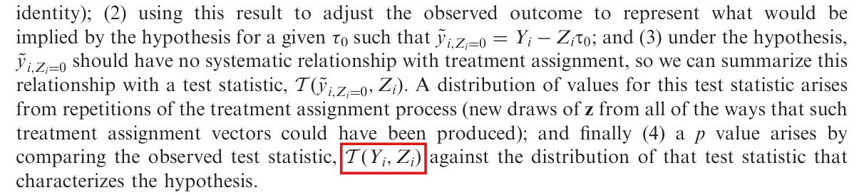
(S2) The testing procedure. p. 396 (PDF p. 2), Section 1: “Say $Y_i$ is the observed outcome, and we hypothesize that units do not interfere and also that $y_{i,Z_i=1} = y_{i,Z_i=0} + \tau$. We can assess which (if any) hypothesized values of $\tau$ appear implausible from the perspective of the data by: (1) mapping the hypothesis about unobserved quantities to observed data using the identity $Y_i = Z_i y_{i,Z_i=1} + (1 - Z_i) y_{i,Z_i=0}$—noticing that if $y_{i,Z_i=1} = y_{i,Z_i=0} + \tau$ then $y_{i,Z_i=0} = Y_i - Z_i\tau$ (by substituting from the hypothesized relationship into the observed data identity); (2) using this result to adjust the observed outcome to represent what would be implied by the hypothesis for a given $\tau_0$ such that $\tilde y_{i,Z_i=0} = Y_i - Z_i\tau_0$; and (3) under the hypothesis, $\tilde y_{i,Z_i=0}$ should have no systematic relationship with treatment assignment, so we can summarize this relationship with a test statistic, $\mathcal{T}(\tilde y_{i,Z_i=0}, Z_i)$. A distribution of values for this test statistic arises from repetitions of the treatment assignment process (new draws of $\mathbf{z}$ from all of the ways that such treatment assignment vectors could have been produced); and finally (4) a $p$ value arises by comparing the observed test statistic, $\mathcal{T}(Y_i, Z_i)$ against the distribution of that test statistic that characterizes the hypothesis.” The paper gives no formula for the $p$ value and does not say which tail (or tails) of the reference distribution is used.
(S3) The KS statistic. Footnote 3, p. 396 (PDF p. 2): “If the empirical cumulative distribution function (ECDF) of the treated units is $F_1$ and the ECDF of the control units is $F_0$, then the KS test statistic is $\mathcal{T}(\mathbf{y}_0, \mathbf{z})_{\mathrm{KS}} = \max_{i=1,\ldots,n}\left[F_1(y_{i,0}) - F_0(y_{i,0})\right]$, where $F(x) = (1/n)\sum_{i=1}^{n} I(x_i \le x)$ records the proportion of the distribution of $x$ at or below $x_i$ (Hollander 1999, section 5.4).”
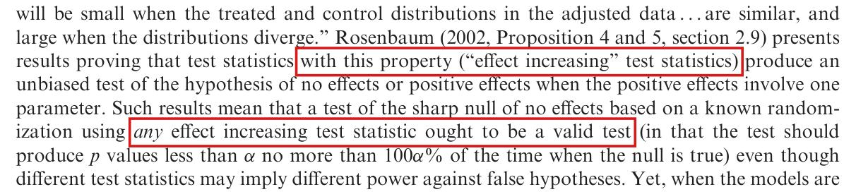
(S4) Validity as the paper states it. p. 397 (PDF p. 3): “Such results mean that a test of the sharp null of no effects based on a known randomization using any effect increasing test statistic ought to be a valid test (in that the test should produce $p$ values less than $\alpha$ no more than $100\alpha\%$ of the time when the null is true) even though different test statistics may imply different power against false hypotheses.”
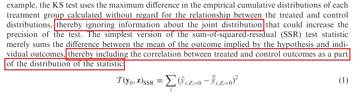
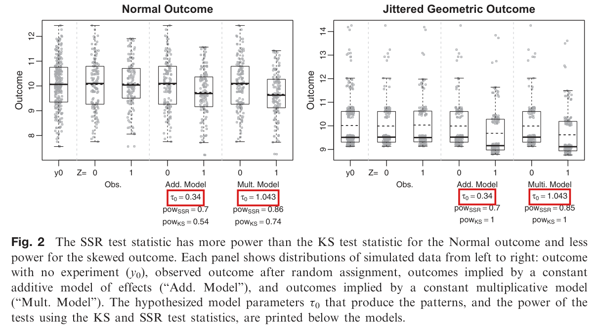
(S5) The simple SSR statistic and the no-interference simulation. p. 397 (PDF p. 3), Section 2: “For example, the implication of the constant, additive effects model, $\tilde y_{i,Z_i=0} = Y_i - Z_i\tau$, only changes the distribution of outcomes for units in the treated condition.” Equation (1), with the sentence that introduces it: “The simplest version of the sum-of-squared-residual (SSR) test statistic merely sums the difference between the mean of the outcome implied by the hypothesis and individual outcomes, thereby including the correlation between treated and control outcomes as a part of the distribution of the statistic: $$\mathcal{T}(\mathbf{y}_0, \mathbf{z})_{\mathrm{SSR}} \equiv \sum_i \left(\tilde y_{i,Z_i=0} - \bar{\tilde y}_{i,Z_i=0}\right)^2 \quad (1)$$” Design: “we created a small simulation study of 256 units with half assigned to a binary treatment completely at random. We compared the performance of the two test statistics on two outcomes with no interference—a Normal outcome and a skewed outcome, both with mean of 10 and standard deviation of 1, as shown in Fig. 1.” Models: “We compared two models of effects—a constant additive effects model in which $y_{i,Z_i=1} = y_{i,Z_i=0} + \tau$ and a constant multiplicative effects model in which $y_{i,Z_i=1} = y_{i,Z_i=0} \cdot \tau$. We set the truth to be the sharp null of no effects such that the true $\tau = 0$ for the additive model and the true $\tau = 1$ for the multiplicative model.”
(S6) The SSR statistic with network information. p. 399 (PDF p. 5), Section 2.1: “In the case where we know the fixed binary adjacency matrix of a social network, $\mathbf{S}$, where a given entry in the $n \times n$ matrix is 1 if two units are adjacent and 0 if two units are not adjacent, and where we imagine that network attributes (like degree) of a node play a role in the mechanism by which treatment propagates, the idea of assessing model fit rather than closeness of distributions leads naturally to the SSRs from a least squares regression of $\tilde y_{i,Z_i=0}$ on $Z_i$ and $\mathbf{z}^T\mathbf{S}$ (i.e., the number of directly connected nodes assigned treatment) as well as the $\mathbf{1}^T\mathbf{S}$ (i.e., the degree of the node). If we collected $Z_i$, $\mathbf{z}^T\mathbf{S}$, and $\mathbf{1}^T\mathbf{S}$ into a matrix $\mathbf{X}$, and fit the $\tilde y_{i,Z_i=0}$ as a linear function of $\mathbf{X}$ with fitted coefficients $\hat{\boldsymbol\beta}$ then we could define the test statistic as $$\mathcal{T}(y_0, \mathbf{z})_{\mathrm{SSR}} \equiv \sum_i \left(\tilde y_{i,Z_i=0} - \mathbf{X}\hat{\boldsymbol\beta}\right)^2. \quad (2)$$” (In display (2) the first argument is printed as an italic $y_0$; in display (1) and in footnote 3 it is a bold $\mathbf{y}_0$.)
(S7) The network model, design and tests. p. 399 (PDF p. 5), Section 2.2: “Their model of treatment propagation was $$\mathcal{H}(\mathbf{y}_{\mathbf{z}}, \mathbf{w}, \beta, \tau) = \frac{\beta + (1 - w_i)(1 - \beta)\exp(-\tau^2\mathbf{w}^T\mathbf{S})}{\beta + (1 - z_i)(1 - \beta)\exp(-\tau^2\mathbf{z}^T\mathbf{S})}\,\mathbf{y}_{\mathbf{z}}. \quad (3)$$ Briefly, this model posits that treatment effects can depend on either direct assignment to treatment ($\mathbf{z}$) governed by $\beta$ or spillover as an increasing (but flattening) function of the number of directly connected treated neighbors ($\mathbf{z}^T\mathbf{S}$) and is governed by $\tau$. So, we have a model with two parameters. The network used by BFP involves 256 nodes connected in an undirected, random graph with node degree ranging from 0 to 10 (mean degree 4, 95% of nodes with degree between 1 and 8, five unconnected nodes with degree 0). Treatment is assigned to 50% of the nodes completely at random in the BFP example.” pp. 399–400 (PDF pp. 5–6): “We assess three versions of the SSR test statistic versus three versions of the KS test statistic. The first, described above, we call the SSR + Design test statistic because it represents information about how treatment is assigned to the nodes, $\mathbf{z}^T\mathbf{S}$. The second version of the SSR test statistic (SSR + Degree) only includes network degree, $\mathbf{1}^T\mathbf{S}$, and excludes information about the treatment status of other nodes. And the third version (SSR) includes only treatment assignment $\mathbf{z}$.” p. 400: “For each test statistic, we tested the hypothesis $\tau = \tau_0, \beta = \tau_0$ by using a simulated permutation test: we sampled 1000 permutations. We executed that test 10,000 times for each pair of parameters. The proportion of $p$ values from that test less than .05 is plotted in Fig. 3: darker values show fewer rejections, lighter values record more rejections.” p. 400: “The KS + Design and KS + Degree panels show the power of applying the KS test to residuals from linear models including network degree only (the + Degree version) or degree and also the number of treated neighbors (the +Design version).” Fig. 3 caption, p. 401 (PDF p. 7): “Proportion of $p$ values less than .05 for tests of joint hypotheses about $\tau$ and $\beta$ for the model in equation (3). Darker values mean rare rejection. White means rejection always. Truth is shown at the intersection of the straight lines $\tau = .5, \beta = 2$. Each panel shows a different test statistic. The SSR tests refer to equation (2), the KS tests refer to the expression in footnote 3.”
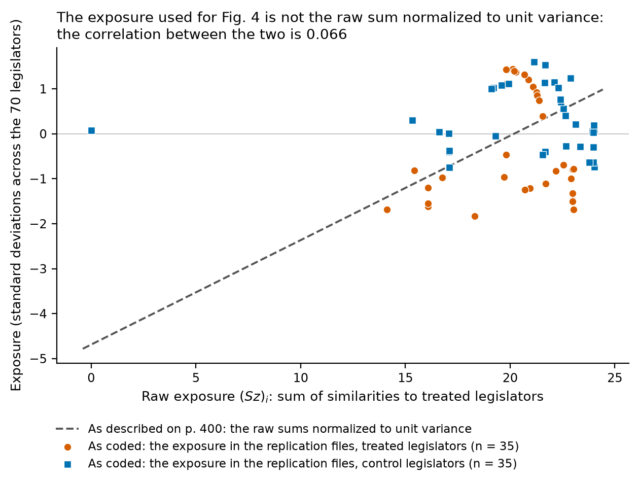
(S8) The application model. p. 400 (PDF p. 6), Section 3: “Coppock reanalyzes the experimental results with an eye toward spillover, constructing a social network based on similarity on W-NOMINATE ideology scores. Coppock hypothesized that ideologically similar legislators would be more likely to share information.” “With distance matrix $\Gamma$, Coppock evaluated the model: $$\mathbf{y}_0 = \mathbf{y}_{\mathbf{z}} - \beta_1\mathbf{z} - \beta_2 g(\Gamma\mathbf{z}),$$ where $g$ is a function that normalizes the sums of distances to treated neighbors to have unit variance. This model has a direct effect ($\beta_1$) and an indirect effect ($\beta_2$) that is linear in the distances to treated neighbors. Coppock evaluated this spillover model using the SSR + Design statistic as presented in this article.”
(S9) Conventions of this list (not the paper's notation). In the targets, $u \in \mathbb{R}^n$ (or $a$) is the vector of hypothesis-adjusted outcomes $u_i = \tilde y_{i,Z_i=0}$, held fixed while the assignment is redrawn; $z \in \{0,1\}^n$ is an assignment with $n_g = \#\{i : z_i = g\}$ units in group $g$ ($g = 1$ treated, $g = 0$ control); $\bar u_g$ or $m_g$ is the mean of $u$ over group $g$; $R(u,z) = \sum_i (u_i - \bar u_{z_i})^2$ is the residual sum of squares from the least-squares regression of $u$ on an intercept and $z$ (the statistic that the paper calls ‘SSR’, as the released code computes it); $F_g(t) = n_g^{-1}\#\{i : z_i = g,\ u_i \le t\}$ and $D(u,z) = \max_i |F_1(u_i) - F_0(u_i)|$ is the two-sided KS distance (as the released code computes it). The expressions $\mathbf{z}^T\mathbf{S}$ and $\mathbf{1}^T\mathbf{S}$ in displays (2) and (3) are read componentwise: for unit $i$, $(z^TS)_i = \sum_j z_j S_{ji}$ (the number of treated neighbours) and $(1^TS)_i = \sum_j S_{ji}$ (the degree). A randomization design is a probability distribution on a finite set $\Omega \subseteq \{0,1\}^n$ of assignments; ‘completely at random’ with half treated is read as the uniform distribution on the assignments with exactly $n/2$ treated units. Witnesses and corrected statements are the validators' and Sol's constructions unless a passage is marked as printed.
Effective claim (source TeX): Exact witnesses (the validators' constructions; not in the paper) that the exposure used by the released application code is not a centring and rescaling of the sums of similarities, or of distances, to treated units, even allowing a changed intercept and a changed own-treatment coefficient; and that the rejection rule of the released simulation code differs from the printed one.
Notation (the released code's operations, written out in P016-T4). For scores $s \in \mathbb{R}^n$: $S_{ij} = 1 - |s_i - s_j|/2$ for $i \ne j$ and $S_{ii} = 0$ (similarity); $D_{ij} = |s_i - s_j|$ (distance). For a finite bank $\mathcal{B}$ of assignments, $\mu_{ia}$ is the average of $(Sz')_i$ over the bank assignments $z'$ with $z'_i = a$, and $h_i(z) = (Sz)_i - z_i\mu_{i1} - (1 - z_i)\mu_{i0}$. The code's exposure $e(z)$ is $h(z)$ centred at its mean over units and divided by its sample standard deviation over units.
(i) [Four units] $s = (-1, -\tfrac12, \tfrac12, 1)$, so $$S = \begin{pmatrix} 0 & 3/4 & 1/4 & 0 \\ 3/4 & 0 & 1/2 & 1/4 \\ 1/4 & 1/2 & 0 & 3/4 \\ 0 & 1/4 & 3/4 & 0 \end{pmatrix}.$$ The bank is the whole matched-pair design: the four assignments $(0,1,0,1), (0,1,1,0), (1,0,0,1), (1,0,1,0)$ that treat exactly one unit in each of the pairs $\{1,2\}$ and $\{3,4\}$. Then $(\mu_{i0}, \mu_{i1}) = (\tfrac78, \tfrac18), (\tfrac98, \tfrac38), (\tfrac98, \tfrac38), (\tfrac78, \tfrac18)$ for $i = 1,2,3,4$. At $z = (1,0,1,0)$: $x := Sz = (\tfrac14, \tfrac54, \tfrac14, \tfrac34)$, $Dz = (\tfrac32, \tfrac32, \tfrac32, \tfrac52)$ and $h(z) = (\tfrac18, \tfrac18, -\tfrac18, -\tfrac18)$. There are no real numbers $A, B, C$ with $h_i(z) = A + Bz_i + Cx_i$ for $i = 1,\ldots,4$, and none with $h_i(z) = A + Bz_i + C(Dz)_i$ for $i = 1,\ldots,4$ (units 1 and 3 are both treated and have $x_1 = x_3$ and $(Dz)_1 = (Dz)_3$, but $h_1 \ne h_3$); the $4 \times 4$ matrix with rows $(1, z_i, x_i, h_i(z))$ has determinant $\tfrac18 \ne 0$.
(ii) [Six units, with the statistic] $s = (-1, -\tfrac34, -\tfrac12, 0, \tfrac14, 1)$, so $$S = \frac18\begin{pmatrix} 0&7&6&4&3&0\\ 7&0&7&5&4&1\\ 6&7&0&6&5&2\\ 4&5&6&0&7&4\\ 3&4&5&7&0&5\\ 0&1&2&4&5&0 \end{pmatrix}.$$ The bank is the whole matched-pair design: the eight assignments $(a, 1-a, b, 1-b, c, 1-c)$, $(a,b,c) \in \{0,1\}^3$. At $z = (1,0,1,0,1,0)$: $x = Sz = (\tfrac98, \tfrac94, \tfrac{11}{8}, \tfrac{17}{8}, 1, \tfrac78)$, $(\mu_{i z_i})_i = (\tfrac{13}{16}, \tfrac{31}{16}, \tfrac54, 2, \tfrac{19}{16}, \tfrac{17}{16})$, $h(z) = (\tfrac{5}{16}, \tfrac{5}{16}, \tfrac18, \tfrac18, -\tfrac{3}{16}, -\tfrac{3}{16})$, with mean $\tfrac1{12}$ and sample variance $\tfrac{49}{960}$, so that $e(z) = \tfrac{\sqrt{15}}{42}(11, 11, 2, 2, -13, -13)$. There are no real $A, B$ with $h(z) = A + Bx$ and no real $A, B, C$ with $h_i(z) = A + Bz_i + Cx_i$ for all $i$ (units 1 and 3 force $C = -\tfrac34$; units 2 and 4 force $C = \tfrac32$). For $y = (0,1,0,1,1,0)$ and $d = S\mathbf{1} = (\tfrac52, 3, \tfrac{13}{4}, \tfrac{13}{4}, 3, \tfrac32)$, the residual sum of squares of the least-squares regression of $y$ is $\tfrac43$ on the columns $(1, z, h(z))$ (the released code's statistic; the same with $e(z)$ in place of $h(z)$), $\tfrac{655}{708}$ on the columns $(1, z, x)$ (raw similarity sums) and $\tfrac{515}{859}$ on the columns $(1, z, x, d)$ (raw sums and the degree analogue).
(iii) [The staged application table] The first four rows of the released table CoppockJEPS.tab record treatment $Z$, raw exposure $x$ (column exposure.observed.dw) and corrected exposure $h$ (column difs.dw) as $(0,\ 21.6630956840236,\ 0.370753999962044)$, $(0,\ 19.1947426509578,\ 0.240866262449021)$, $(1,\ 20.8676713418681,\ 0.286925998351727)$, $(1,\ 22.5467332911212,\ -0.193126413625389)$. Reading these decimals as exact rationals, the $4 \times 4$ matrix with rows $(1, Z, x, h)$ has determinant $$-\frac{14030283848669586515272953541}{10^{28}} \ne 0,$$ so in the application's own data $h$ is not of the form $A + BZ + Cx$.
(iv) [The cutoff, and the tails] For reference statistics $T_1,\ldots,T_B$ and observed statistic $T_{\mathrm{obs}}$ put $L = \#\{b : T_b \le T_{\mathrm{obs}}\}/B$, $U = \#\{b : T_b \ge T_{\mathrm{obs}}\}/B$ and $p_2 = \min\{1, 2\min(L,U)\}$ (the simulation code's $p$ value). With $B = 1000$ and $T_b = b$: at $T_{\mathrm{obs}} = 25$, $L = \tfrac1{40}$, $U = \tfrac{122}{125}$ and $p_2 = \tfrac1{20}$, so the code's rule $p_2 \le .05$ rejects and the printed rule $p_2 < .05$ does not; at $T_{\mathrm{obs}} = 40$, $L = \tfrac1{25} \le .05$ but $p_2 = \tfrac2{25} > .05$; at $T_{\mathrm{obs}} = 980$, $L = \tfrac{49}{50} > .05$ but $p_2 = \tfrac{21}{500} \le .05$. Hence the lower-tail rule (used for SSR in the application) and the two-sided rule (used in the simulations) have rejection regions neither of which contains the other.
: T3Statement
Theorem: SAP.P016a.T3
Statement hash: 57bddc4c9d8c7cdc15c3950d36b9847bb929b5fd12ef0b2048422e7fe8163a48
Statement definition: SAP.P016a.T3Statement
Certificate. 20261104T104233Z
Declaration review: faithful; 2026-11-04T11:59:39Z; binding v2
Declaration review: faithful; 2026-11-04T16:21:21Z; binding v2
Evidence scope: Certification checks formal proof objects. Statement fidelity is a model judgment. Author review is separate.
Proof dependencies: Independently extracted
Source and evidence metadata · sap-2026-11-08-assured-release