LLM-generated corrections to the published research of P. M. Aronow

Journal article P017

Corrections to: Data-Adaptive Causal Effects and Superefficiency

P. M. Aronow (2016). Data-Adaptive Causal Effects and Superefficiency. Journal of Causal Inference 4(2).

DOI
10.1515/jci-2016-0007
arXiv
1601.01413
Audited edition
Journal of Causal Inference, 2016, 4(2); 4 pages in the audited file
SHA-256 of the audited file
90a89bc1f401886c4fef400a270ce6200153837d322217746bfe4b68bb47a88e
Permanent address
https://pmaronow.github.io/llm-audit/works/P017/

Summary

This four-page note asks how much precision is gained when the target of inference may depend on the data. It clips a root-nn consistent and asymptotically normal estimator of the average causal effect to an interval determined by the support of the effects, takes the clipped value as the target, and shows that the estimator is superefficient for this target. 5 entries are classified as errors (1 Moderate, 4 Minor), and 1 is a clarity note. The most important is P017-E001: this target is not a weighted average of causal effects in every realization.

What was and was not checked

I read the whole text of the note and every proof. The following were checked and held up.

  • Assumption 1 holds if and only if τ\tau is not constant, where c=+∞c=+\infty is allowed.
  • Definition 2: the three cases are exhaustive and mutually exclusive, and the target is θ^\hat\theta clipped to [EG[τ]−c, EG[τ]+c][\mathrm{E}_G[\tau]-c,\ \mathrm{E}_G[\tau]+c].
  • Proposition 2 and its proof: ∣θFn−EG[τ]∣≤∣θ^−EG[τ]∣|\theta_{F_n}-\mathrm{E}_G[\tau]|\le|\hat\theta-\mathrm{E}_G[\tau]| in every realization.
  • The statements of Propositions 3 and 4, by the arguments given in P017-E002. Assumption 1 is needed in Proposition 3.
  • The statement of Corollary 1, and the remarks that its condition holds when Supp⁡G[τ]=R\operatorname{Supp}_G[\tau]=\mathbb{R} and that its conclusion fails when Supp⁡G[τ]=R+\operatorname{Supp}_G[\tau]=\mathbb{R}^+ and Pr⁡(θ^<0)>0\Pr(\hat\theta<0)>0.
  • The closed-form evaluation of the Gaussian tail integral in the proof of Proposition 4, by integration by parts and by numerical integration.
  • Proposition 1 for every target that lies strictly between the infimum and the supremum of the support of τ\tau or equals an endpoint of positive probability, and hence in every realization when τ\tau has finite support or support unbounded in both directions.
  • The statement in the discussion that the gains “may be essentially unbounded”, which agrees with θ^−θFn=op(an)\hat\theta-\theta_{F_n}=o_p(a_n) for every positive sequence (an)(a_n).
  • The cross-references to the numbered assumption, definitions, propositions and corollary, and the citation numbers 1 to 10, which all resolve.
  • The page cited for the quotation from Crump et al. in Section 3 and the details of references 1 and 10, against public sources (P017-N003).

I did not compare the descriptions of the cited works in the introduction with those works, or references 2 to 9 with outside sources. The note has no tables, figures or appendix; I had no supplement, replication files or correction notice to examine. That no correction is listed here for a passage does not show that the passage is correct.

Headline claims and related corrections

  1. Under Assumption 1, with heterogeneous effects and c>0c>0, any estimator of the population average causal effect that is consistent at rate n−1/2n^{-1/2} and asymptotically normal is superefficient for the data-adaptive target: n(θ^−θFn)=op(1)\sqrt{n}(\hat\theta-\theta_{F_n})=o_p(1).

    Proposition 3 (with Assumption 1 and Definitions 1-2); abstract; introduction; Section 3

    See P017-E001, P017-E002, P017-E003, P017-N001.

  2. The data-adaptive target θFn\theta_{F_n} is claimed to be a local average causal effect in every realization: there is a nonnegative weighting wFnw_{F_n} with θFn=EG[wFnτ]/EG[wFn]\theta_{F_n}=\mathrm{E}_G[w_{F_n}\tau]/\mathrm{E}_G[w_{F_n}], so the target is the average effect of at least one subpopulation.

    Proposition 1; Definition 2; abstract and introduction ('a data-adaptive local average causal effect')

    See P017-E001.

  3. The data-adaptive target converges to the population average causal effect at rate n−1/2n^{-1/2}: n(θFn−EG[τ])=Op(1)\sqrt{n}(\theta_{F_n}-\mathrm{E}_G[\tau])=O_p(1).

    Proposition 2

  4. Under Assumption 1, if n(θ^−EG[τ])=Zn+εn\sqrt{n}(\hat\theta-\mathrm{E}_G[\tau])=Z_n+\varepsilon_n, where Zn∼N(0,σ2)Z_n\sim N(0,\sigma^2) with 0<σ2<∞0<\sigma^2<\infty and E[εn2]=o(n−1/2)\mathrm{E}[\varepsilon_n^2]=o(n^{-1/2}), the mean square error of θ^\hat\theta for the data-adaptive target is o(n−1)o(n^{-1}).

    Proposition 4 and its displayed normal-tail calculation; introduction, last sentence

    See P017-E001, P017-E002, P017-E004.

  5. Adapting the target on the basis of efficiency can deliver extraordinary precision gains; without further restrictions the gains in statistical certainty 'may be essentially unbounded', and in the support-containment case the estimator has zero error for the adaptive target in every realization.

    Proposition 3 and its proof (op(an)o_p(a_n) for every positive deterministic sequence (an)(a_n)); Corollary 1; abstract; Section 3

    See P017-E004, P017-N001.

  6. The efficiency gain can come at the cost of a target of little intrinsic interest and a subpopulation whose composition is unknown to the researcher; restrictions on adaptive targets may therefore be warranted.

    Section 3, second paragraph; Definition 2; Proposition 1 and the paragraph after its proof; Corollary 1

Corrections

Moderate (1)

A real substantive error with limited reach.

Proposition 1 fails when the target of Definition 2 is an endpoint of the support of τ\tau that has probability zero; with a fixed clipping radius 0<d<c0<d<c in place of cc, the target is a nonnegative weighted average of causal effects for every empirical distribution.

Definition 2 and Proposition 1, PDF p. 2 (the pages are not numbered), with the proof sentence and the explanation that follow Proposition 1

See also under Formal statements (Lean): P017-T1, P017-T2, P017-T3, P017-T4, P017-T9

My comment on this entry

As printed

Definition 2: Let the target parameter

θFn={θ^: ∣θ^−EG[τ]∣≤cEG[τ]+c: θ^−EG[τ]>cEG[τ]−c: θ^−EG[τ]<−c,\theta_{F_n}=\begin{cases}\hat\theta & :\ |\hat\theta-\mathrm{E}_G[\tau]|\le \colorbox{#ffe58a}{$\displaystyle c$}\\ \mathrm{E}_G[\tau]+\colorbox{#ffe58a}{$\displaystyle c$} & :\ \hat\theta-\mathrm{E}_G[\tau]>\colorbox{#ffe58a}{$\displaystyle c$}\\ \mathrm{E}_G[\tau]-\colorbox{#ffe58a}{$\displaystyle c$} & :\ \hat\theta-\mathrm{E}_G[\tau]<-\colorbox{#ffe58a}{$\displaystyle c$}\end{cases},

where, as in Assumption 1, c=min⁡(sup⁡(Supp⁡G[τ])−EG[τ], EG[τ]−inf⁡(Supp⁡G[τ]))c=\min(\sup(\operatorname{Supp}_G[\tau])-\mathrm{E}_G[\tau],\ \mathrm{E}_G[\tau]-\inf(\operatorname{Supp}_G[\tau])).

The target parameter adapts naturally to the closest value in an interval surrounding EG[τ]\mathrm{E}_G[\tau], where the width of the interval is defined by the support of τ\tau. We formalize how each θFn\theta_{F_n} is a local average treatment effect.

Proposition 1: There exists a nonnegative weighting associated with each empirical distribution FnF_n, wFnw_{F_n}, such that across all FnF_n, θFn=EG[wFnτ]EG[wFn]\theta_{F_n}=\frac{\mathrm{E}_G[w_{F_n}\tau]}{\mathrm{E}_G[w_{F_n}]}.

A proof of Proposition 1 follows directly from the fact that a weighted mean can obtain any value in the interval defined by the infimum and supremum of its distribution’s support. Proposition 1 asserts that across all realizations, the target parameter θFn\theta_{F_n} corresponds to an average causal effect for at least one subpopulation.

The problem

Proposition 1 asserts that, for every empirical distribution FnF_n, the target θFn\theta_{F_n} of Definition 2 equals EG[wτ]/EG[w]\mathrm{E}_G[w\tau]/\mathrm{E}_G[w] for some nonnegative weighting ww. Definition 2 clips θ^\hat\theta to the closed interval [EG[τ]−c, EG[τ]+c][\mathrm{E}_G[\tau]-c,\ \mathrm{E}_G[\tau]+c]. When cc is finite, at least one end of this interval is the infimum or the supremum of the support of τ\tau, and the target equals that value whenever θ^\hat\theta lies at or beyond it. A weighted mean with nonnegative weights attains every value strictly between the infimum and the supremum of the support, but it attains a finite endpoint only if the endpoint has positive probability. The fact given as the proof of Proposition 1 includes the endpoints without this condition. If, for example, τ\tau is bounded and has a continuous distribution, the endpoint has probability zero. On the realizations where θ^\hat\theta lies at or beyond it, the target is a value that no weighting attains, and it is not the average causal effect of any subpopulation. These realizations have probability tending to zero as n→∞n\to\infty, but in the example below they have positive probability at every sample size. The abstract, the introduction and the discussion describe the target as a local average causal effect, and that description depends on Proposition 1.

Evidence a historical Lean attribution (Generated status: clause support not certified in this release)

The evidence is a derivation and an exact counterexample. The obstruction at an endpoint also has a Lean proof.

The values that a weighted mean attains. I call a weighting admissible if it is a measurable function w≥0w\ge0 of the full data such that 0<EG[w]<∞0<\mathrm{E}_G[w]<\infty and EG[∣wτ∣]<∞\mathrm{E}_G[|w\tau|]<\infty. Let tt be a real number. If p0=Pr⁡G(τ=t)>0p_0=\Pr_G(\tau=t)>0, then the weighting w=1{τ=t}/p0w=\mathbf{1}\{\tau=t\}/p_0 satisfies EG[w]=1\mathrm{E}_G[w]=1 and EG[wτ]=t\mathrm{E}_G[w\tau]=t. Suppose next that p−=Pr⁡G(τ<t)>0p_-=\Pr_G(\tau<t)>0 and p+=Pr⁡G(τ>t)>0p_+=\Pr_G(\tau>t)>0, and set

m−=EG[τ1{τ<t}]p−,m+=EG[τ1{τ>t}]p+,a=m+−tm+−m−.m_-=\frac{\mathrm{E}_G[\tau\mathbf{1}\{\tau<t\}]}{p_-},\qquad m_+=\frac{\mathrm{E}_G[\tau\mathbf{1}\{\tau>t\}]}{p_+},\qquad a=\frac{m_+-t}{m_+-m_-}.

Then m−<t<m+m_-<t<m_+ and 0<a<10<a<1. The weighting

w=ap−1{τ<t}+1−ap+1{τ>t}w=\frac{a}{p_-}\mathbf{1}\{\tau<t\}+\frac{1-a}{p_+}\mathbf{1}\{\tau>t\}

is bounded and nonnegative. Computing the two expectations, I find EG[w]=a+(1−a)=1\mathrm{E}_G[w]=a+(1-a)=1 and EG[wτ]=am−+(1−a)m+=t\mathrm{E}_G[w\tau]=am_-+(1-a)m_+=t. Conversely, suppose that Pr⁡G(τ=t)=0\Pr_G(\tau=t)=0 and Pr⁡G(τ>t)=0\Pr_G(\tau>t)=0, so that τ<t\tau<t almost surely. If an admissible weighting ww had weighted mean tt, then EG[w(t−τ)]=t EG[w]−EG[wτ]=0\mathrm{E}_G[w(t-\tau)]=t\,\mathrm{E}_G[w]-\mathrm{E}_G[w\tau]=0. Since w(t−τ)≥0w(t-\tau)\ge0, this implies that w(t−τ)=0w(t-\tau)=0 almost surely. Since t−τ>0t-\tau>0 almost surely, I have w=0w=0 almost surely, which contradicts EG[w]>0\mathrm{E}_G[w]>0. The case Pr⁡G(τ<t)=0\Pr_G(\tau<t)=0 is the same, with w(τ−t)w(\tau-t) in place of w(t−τ)w(t-\tau). I conclude that an admissible weighting with weighted mean tt exists if and only if

Pr⁡G(τ=t)>0,orPr⁡G(τ<t)>0  and  Pr⁡G(τ>t)>0.\Pr_G(\tau=t)>0,\quad\text{or}\quad \Pr_G(\tau<t)>0\ \text{ and }\ \Pr_G(\tau>t)>0.

Every tt strictly between the infimum and the supremum of the support of τ\tau satisfies the second condition. A finite endpoint of the support satisfies neither condition unless it has positive probability.

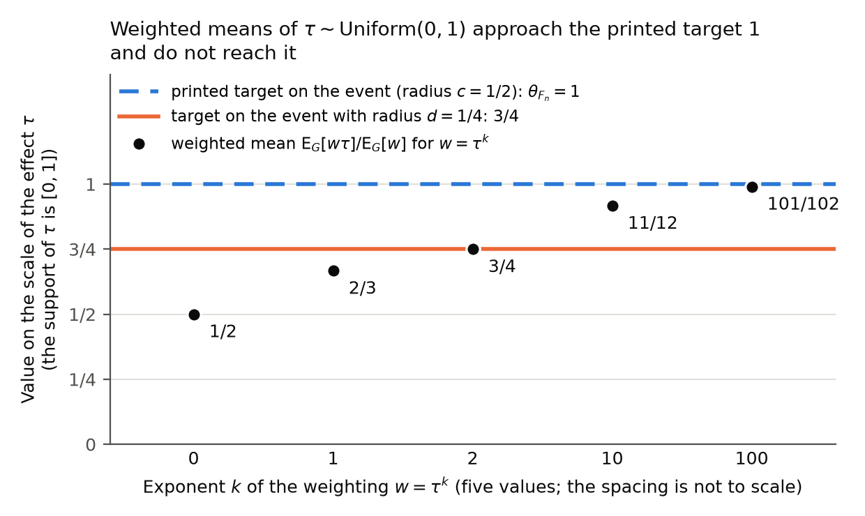
The counterexample. Let τ\tau be uniform on (0,1)(0,1), let BB equal −1-1 or 11 with probability 1/21/2 each, and let TT be a fair treatment assignment, with τ\tau, BB and TT independent. Let Y(0)=BY(0)=B, Y(1)=B+τY(1)=B+\tau and Y=TY(1)+(1−T)Y(0)Y=TY(1)+(1-T)Y(0). Then EG[τ]=1/2\mathrm{E}_G[\tau]=1/2, the support of τ\tau is [0,1][0,1] and c=1/2c=1/2, so that Definition 2 clips θ^\hat\theta to [0,1][0,1]. For nn independent units, I take the inverse-probability estimator θ^=n−1∑i=1nXi\hat\theta=n^{-1}\sum_{i=1}^nX_i with Xi=2TiYi−2(1−Ti)YiX_i=2T_iY_i-2(1-T_i)Y_i. The summands are bounded, with mean 1/21/2 and variance 53/1253/12. By the central limit theorem, I have n(θ^−1/2)⇒N(0,53/12)\sqrt n(\hat\theta-1/2)\Rightarrow N(0,53/12). On the event that (Ti,Yi)=(0,−1)(T_i,Y_i)=(0,-1) for all ii, every XiX_i equals 22, and therefore θ^=2\hat\theta=2 and θFn=1\theta_{F_n}=1. Since τ<1\tau<1 almost surely, no admissible weighting has weighted mean 11, by the characterization above.

The counterexample to Proposition 1, with τ\tau uniform on (0,1)(0,1). All values are exact.
QuantityValue
EG[τ]\mathrm{E}_G[\tau] and cc1/21/2 and 1/21/2
Mean and variance of XiX_i1/21/2 and 53/1253/12
Probability that (Ti,Yi)=(0,−1)(T_i,Y_i)=(0,-1) for every ii4−n4^{-n}
Estimate θ^\hat\theta on this event22
Printed target θFn\theta_{F_n} on this event11
Target on this event with radius d=1/4d=1/43/43/4

The Lean proof covers the following statement: for an integrable weighting w≥0w\ge0 with positive expectation, on a population in which τ<1\tau<1 almost surely and wτw\tau is integrable, the weighted mean is less than 11. It also covers the uniform distribution on (0,1)(0,1), for which the value obtained by clipping the estimate 22 to [0,1][0,1] has no such representation. The Lean statements also specify the Gaussian limit, the probability 4−n4^{-n} of this event at every n≥1n\ge1, and the identity expressing the estimator as an integral against the empirical distribution of the observed pairs. A second example has a failure event of probability 16−n16^{-n}: its effect is discrete, with values that accumulate at −1-1 and 11 and do not reach them.

What survives

The conclusions of Propositions 2, 3 and 4 and the equality Pr⁡(θ^=θFn)=1\Pr(\hat\theta=\theta_{F_n})=1 of Corollary 1 hold for the target as printed, since they can be derived without Proposition 1. Proposition 1 holds as printed when τ\tau has finite support or support unbounded in both directions, and for the printed target the weighted representation exists with probability tending to one. The statement that the printed target is a local average causal effect in every realization does not survive; in particular, under the hypothesis of Corollary 1 the common value of θ^\hat\theta and θFn\theta_{F_n} need not be a weighted average of causal effects. With the radius dd the target differs from the printed one on the realizations with ∣θ^−EG[τ]∣>d|\hat\theta-\mathrm{E}_G[\tau]|>d. No new assumption on GG is needed, the conclusions of Propositions 2, 3 and 4 hold with dd in place of cc, and the claim that θ^\hat\theta is superefficient for a data-adaptive local average causal effect stands.

Corrected

Definition 2: Let cc be as in Assumption 1, and fix a finite radius dd such that 0<d<c0<d<c. Let the target parameter

θFn={θ^: ∣θ^−EG[τ]∣≤dEG[τ]+d: θ^−EG[τ]>dEG[τ]−d: θ^−EG[τ]<−d.\theta_{F_n}=\begin{cases}\hat\theta & :\ |\hat\theta-\mathrm{E}_G[\tau]|\le \colorbox{#ffe58a}{$\displaystyle d$}\\ \mathrm{E}_G[\tau]+\colorbox{#ffe58a}{$\displaystyle d$} & :\ \hat\theta-\mathrm{E}_G[\tau]>\colorbox{#ffe58a}{$\displaystyle d$}\\ \mathrm{E}_G[\tau]-\colorbox{#ffe58a}{$\displaystyle d$} & :\ \hat\theta-\mathrm{E}_G[\tau]<-\colorbox{#ffe58a}{$\displaystyle d$}\end{cases}.

Proposition 1: Suppose that τ\tau has finite expectation and that Assumption 1 holds. There exists a nonnegative weighting associated with each empirical distribution FnF_n, wFnw_{F_n}, with 0<EG[wFn]<∞0<\mathrm{E}_G[w_{F_n}]<\infty and EG[∣wFnτ∣]<∞\mathrm{E}_G[|w_{F_n}\tau|]<\infty, such that across all FnF_n, θFn=EG[wFnτ]EG[wFn]\theta_{F_n}=\frac{\mathrm{E}_G[w_{F_n}\tau]}{\mathrm{E}_G[w_{F_n}]}.

A proof of Proposition 1 follows from the fact that a weighted mean with nonnegative weights can obtain every value strictly between the infimum and supremum of its distribution’s support, and obtains a finite endpoint of the support if and only if that endpoint has positive probability. Since d<cd<c, every value in [EG[τ]−d, EG[τ]+d][\mathrm{E}_G[\tau]-d,\ \mathrm{E}_G[\tau]+d] lies strictly between the infimum and the supremum of the support of τ\tau. Proposition 1 asserts that across all realizations, the target parameter θFn\theta_{F_n} corresponds to an average causal effect for at least one subpopulation.

The later conditions on the target use dd in place of cc; in particular, the hypothesis of Corollary 1 becomes d≥max⁡(sup⁡(Supp⁡[θ^])−EG[τ], EG[τ]−inf⁡(Supp⁡[θ^]))d\ge\max(\sup(\operatorname{Supp}[\hat\theta])-\mathrm{E}_G[\tau],\ \mathrm{E}_G[\tau]-\inf(\operatorname{Supp}[\hat\theta])). If the support of τ\tau is unbounded in both directions, then c=+∞c=+\infty, and the printed target θFn=θ^\theta_{F_n}=\hat\theta may be kept.

Alternatively, Definition 2 may be kept with the radius cc and Proposition 1 weakened: the weighting exists for each FnF_n such that θFn\theta_{F_n} lies strictly between the infimum and the supremum of the support of τ\tau, or equals one of them and that value has positive probability under GG. Such a weighting then exists with probability tending to one under the paper’s consistency and heterogeneity assumptions, but need not exist across all realizations.
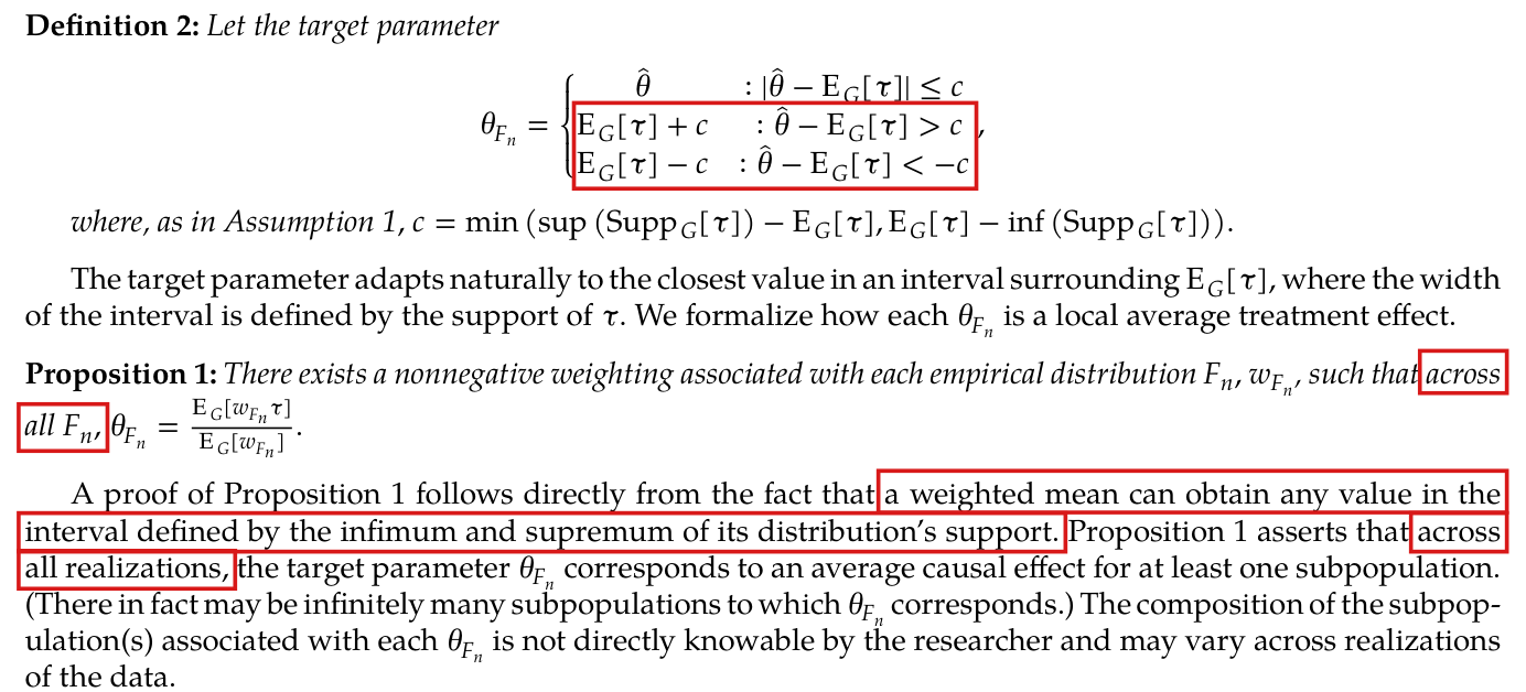
Definition 2 with its display of three cases, the two sentences after it, Proposition 1 and the paragraph that follows. Red boxes mark the second and third cases of the display, 'E_G[tau] + c : theta-hat - E_G[tau] > c' and 'E_G[tau] - c : theta-hat - E_G[tau] < -c'; the words 'across all F_n' in Proposition 1; the words 'a weighted mean can obtain any value in the interval defined by the infimum and supremum of its distribution's support'; and the words 'across all realizations'.
Definition 2, Proposition 1 and the paragraph that follows it, PDF p. 2. The marks show the two cases of Definition 2 in which the target equals EG[τ]+c\mathrm{E}_G[\tau]+c or EG[τ]−c\mathrm{E}_G[\tau]-c, the words “across all FnF_n” in Proposition 1, the fact given as its proof, and the words “across all realizations”.
Chart with the exponent k of the weighting tau to the power k on the horizontal axis, at the five equally spaced labels 0, 1, 2, 10 and 100 (spacing is not to scale), and the value on the scale of the effect on the vertical axis, labelled from 0 to 1. Five black dots show the weighted means 1/2, 2/3, 3/4, 11/12 and 101/102, which rise toward 1. A dashed blue horizontal line at 1 is labelled as the printed target on the event with radius c equal to 1/2; the last dot lies just below it. A solid orange horizontal line at 3/4 is labelled as the target on the event with radius d equal to 1/4; the dot for k equal to 2 lies on it. The title reads 'Weighted means of tau, uniform on (0, 1), approach the printed target 1 and do not reach it'.
The counterexample to Proposition 1, with τ\tau uniform on (0,1)(0,1) and c=1/2c=1/2. On the event that every observation is an untreated unit with outcome −1-1, the printed target is 11 (dashed line). The weightings w=τkw=\tau^k with k=0,1,2,10,100k=0,1,2,10,100 have weighted means 1/21/2, 2/32/3, 3/43/4, 11/1211/12 and 101/102101/102; by the derivation in the text, no admissible weighting has weighted mean 11. With radius d=1/4d=1/4 the target on the same event is 3/43/4 (solid line), which the weighting τ2\tau^2 attains. All values are exact.
My comment and the history of this entry

Agreed. I think this is a fairly minor regularity condition, but it's worth flagging.

  1. Classification before my review (the classification when the audit was first completed, before I reviewed it): Moderate error.
  2. I commented.
  3. Independent evaluation. No change was needed. The entry remains a Moderate error: the printed target can fail to be a weighted causal effect, although the numerical results stand and the repair is routine.

Minor (4)

Real but inconsequential, for example a misprint that does not change a result.

The proofs of Propositions 3 and 4 clip the normal part θ~\tilde\theta where Definition 2 clips θ^\hat\theta; the probability equality, the rate claimed for θ~−θFn\tilde\theta-\theta_{F_n} and the displayed bound on the mean square are false in general, and both propositions hold as stated by a direct clipping argument.

Proof of Proposition 3, PDF p. 2, the claim that (θ~−θFn)(\tilde\theta-\theta_{F_n}) is op(an)o_p(a_n) and the equality that ends in 2Φ(−cn/σ)2\Phi(-c\sqrt n/\sigma); proof of Proposition 4, PDF p. 3, the sentence “Within cc of EG[τ]\mathrm{E}_G[\tau], the squared deviation is zero” and the first line of the display

See also under Formal statements (Lean): P017-T5, P017-T6, P017-T7, P017-T8, P017-T11, P017-T14, P017-T15

As printed

Proof of Proposition 3, PDF p. 2. Proof: Decompose θ^\hat\theta into θ~=N(EG[τ],σ2/n)\tilde\theta=N(\mathrm{E}_G[\tau],\sigma^2/n) and u=op(n−1/2)u=o_p(n^{-1/2}), so that θ^=θ~+u\hat\theta=\tilde\theta+u. Since (θ~−θFn)(\tilde\theta-\theta_{F_n}) is op(an)o_p(a_n) for any positive sequence (an)(a_n), the rate of convergence of θ^\hat\theta is at worst governed by the bound ensured by uu's op(n−1/2)o_p(n^{-1/2}) convergence. To prove the claim, note that for any positive ε\varepsilon, Pr⁡(∣θ~−θFn∣an≥ε)≤Pr⁡(θ~−θFn≠0)=2Φ(−cn/σ)\Pr\left(\frac{|\tilde\theta-\theta_{F_n}|}{a_n}\ge\varepsilon\right)\le\Pr\left(\tilde\theta-\theta_{F_n}\ne0\right)\colorbox{#ffe58a}{$=2\Phi(-c\sqrt n/\sigma)$}, where Φ(.)\Phi(.) denotes the standard Normal CDF. Since lim⁡n→∞2Φ(−cn/σ)=0\lim_{n\to\infty}2\Phi(-c\sqrt n/\sigma)=0, (θ~−θFn)(\tilde\theta-\theta_{F_n}) is op(an)o_p(a_n). Thus θ^−θFn=op(an)+op(n−1/2)=op(n−1/2)\hat\theta-\theta_{F_n}=\colorbox{#ffe58a}{$o_p(a_n)$}+o_p(n^{-1/2})=o_p(n^{-1/2}), yielding the result.

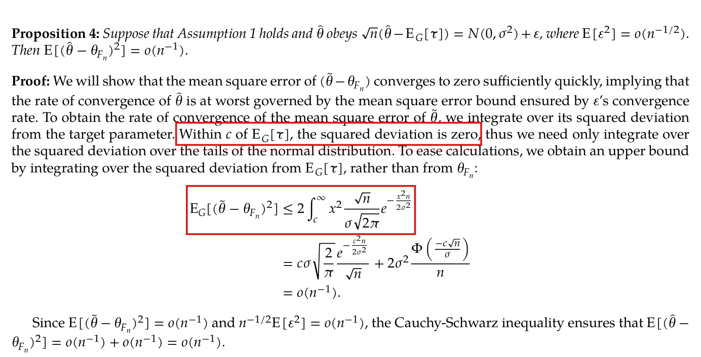
Proof of Proposition 4, PDF p. 3, from its second sentence. To obtain the rate of convergence of the mean square error of θ~\tilde\theta, we integrate over its squared deviation from the target parameter. Within cc of EG[τ]\mathrm{E}_G[\tau], the squared deviation is zero, thus we need only integrate over the squared deviation over the tails of the normal distribution. To ease calculations, we obtain an upper bound by integrating over the squared deviation from EG[τ]\mathrm{E}_G[\tau], rather than from θFn\theta_{F_n}:

EG[(θ~−θFn)2]≤2∫c∞x2nσ2πe−x2n2σ2=cσ2πe−c2n2σ2n+2σ2Φ(−cnσ)n=o(n−1).\begin{aligned} \mathrm{E}_G[(\tilde\theta-\theta_{F_n})^2]&\colorbox{#ffe58a}{$\displaystyle \le$}2\int_c^\infty x^2\frac{\sqrt n}{\sigma\sqrt{2\pi}}e^{-\frac{x^2n}{2\sigma^2}}\\ &=c\sigma\sqrt{\frac{2}{\pi}}\frac{e^{-\frac{c^2n}{2\sigma^2}}}{\sqrt n}+2\sigma^2\frac{\Phi\left(\frac{-c\sqrt n}{\sigma}\right)}{n}\\ &=o(n^{-1}). \end{aligned}
The problem

Definition 2 defines θFn\theta_{F_n} as the clip of the estimator θ^=θ~+u\hat\theta=\tilde\theta+u to the interval [EG[τ]−c, EG[τ]+c][\mathrm{E}_G[\tau]-c,\ \mathrm{E}_G[\tau]+c]. Both proofs compute with the normal part θ~\tilde\theta as though θFn\theta_{F_n} were the clip of θ~\tilde\theta. On the event ∣θ^−EG[τ]∣≤c|\hat\theta-\mathrm{E}_G[\tau]|\le c the target equals θ^\hat\theta, which implies that θ~−θFn=−u\tilde\theta-\theta_{F_n}=-u, and uu is not zero in general. In the proof of Proposition 3, the probability Pr⁡(θ~−θFn≠0)\Pr(\tilde\theta-\theta_{F_n}\ne0) need not equal 2Φ(−cn/σ)2\Phi(-c\sqrt n/\sigma), and θ~−θFn\tilde\theta-\theta_{F_n} need not be op(an)o_p(a_n) for every positive sequence (an)(a_n). In the proof of Proposition 4, the squared deviation need not vanish when ∣θ~−EG[τ]∣≤c|\tilde\theta-\mathrm{E}_G[\tau]|\le c; when ∣θ^−EG[τ]∣≤c|\hat\theta-\mathrm{E}_G[\tau]|\le c, it equals u2u^2. The Gaussian tail integral does not bound E[(θ~−θFn)2]\mathrm{E}[(\tilde\theta-\theta_{F_n})^2] in general. The three steps do hold for some remainders, for instance a remainder that is zero when θ~\tilde\theta is in the interval and moves θ~\tilde\theta away from the interval otherwise. They do not follow from the assumptions of the two propositions. Both propositions are true as stated, but the printed proofs do not establish them.

Evidence an exact counterexample

I give an exact counterexample to the three steps and derive both propositions in the corrected proofs below.

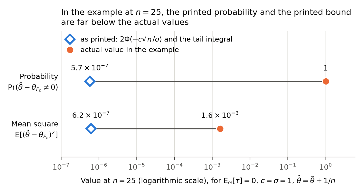
Let the effects equal −1-1 or 11 with probability 1/21/2 each, so that EG[τ]=0\mathrm{E}_G[\tau]=0 and c=1c=1, and let X1,…,XnX_1,\ldots,X_n be independent N(0,1)N(0,1) observations. Set θ~=Xˉn\tilde\theta=\bar X_n and θ^=θ~+1/n\hat\theta=\tilde\theta+1/n. Then σ=1\sigma=1 and u=1/n=op(n−1/2)u=1/n=o_p(n^{-1/2}). Further, n θ^=N(0,1)+ε\sqrt n\,\hat\theta=N(0,1)+\varepsilon with ε=n−1/2\varepsilon=n^{-1/2} and E[ε2]=1/n=o(n−1/2)\mathrm{E}[\varepsilon^2]=1/n=o(n^{-1/2}), and the assumptions of both propositions hold. The difference θ~−θFn\tilde\theta-\theta_{F_n} equals −1/n-1/n when ∣θ^∣≤1|\hat\theta|\le1, and outside this event it vanishes only if θ~=1\tilde\theta=1, which has probability zero. I therefore have Pr⁡(θ~−θFn≠0)=1\Pr(\tilde\theta-\theta_{F_n}\ne0)=1 for all nn, while the printed value is 2Φ(−n)=Pr⁡(∣θ~∣>1)≤1/n2\Phi(-\sqrt n)=\Pr(|\tilde\theta|>1)\le1/n. For n≥2n\ge2, the event ∣θ~∣≤1/2|\tilde\theta|\le1/2 has probability at least 1−4/n1-4/n, and on it θ~−θFn=−1/n\tilde\theta-\theta_{F_n}=-1/n. It follows that n(θ~−θFn)→−1n(\tilde\theta-\theta_{F_n})\to-1 in probability, and θ~−θFn\tilde\theta-\theta_{F_n} is not op(an)o_p(a_n) for an=1/na_n=1/n. At n=25n=25, using the same event, I obtain

E[(θ~−θFn)2]≥1625⋅2125=2115625,\mathrm{E}[(\tilde\theta-\theta_{F_n})^2]\ge\frac{1}{625}\cdot\frac{21}{25}=\frac{21}{15625},

while the printed tail integral equals E[θ~21{∣θ~∣>1}]\mathrm{E}[\tilde\theta^2\mathbf{1}\{|\tilde\theta|>1\}], which is at most E[θ~6]=15/15625\mathrm{E}[\tilde\theta^6]=15/15625. The printed inequality fails by at least 6/156256/15625.

The printed calculations in the counterexample, at n=25n=25 in the first three rows. The mean square values are from numerical integration; decimal values are rounded.
QuantityAs printedIn the example
Pr⁡(θ~−θFn≠0)\Pr(\tilde\theta-\theta_{F_n}\ne0)2Φ(−5)≈5.7×10−72\Phi(-5)\approx5.7\times10^{-7}11
E[(θ~−θFn)2]\mathrm{E}[(\tilde\theta-\theta_{F_n})^2], decimal valueat most 6.2×10−76.2\times10^{-7}1.6×10−31.6\times10^{-3}
E[(θ~−θFn)2]\mathrm{E}[(\tilde\theta-\theta_{F_n})^2], exact boundat most 15/1562515/15625at least 21/1562521/15625
Limit in probability of n(θ~−θFn)n(\tilde\theta-\theta_{F_n})00−1-1

The corrected proofs use three facts. First, Definition 1 implies that n(θ^−EG[τ])=Op(1)\sqrt n(\hat\theta-\mathrm{E}_G[\tau])=O_p(1), and hence that θ^\hat\theta is consistent. Second, the function r(x)=x−C(x)r(x)=x-C(x), where CC is the clip to the interval, is continuous and piecewise linear with slopes 11, 00 and 11, so that ∣r(y)−r(x)∣≤∣y−x∣|r(y)-r(x)|\le|y-x| for all xx and yy. Third, a variable W∼N(0,σ2/n)W\sim N(0,\sigma^2/n) has E[W4]=3σ4/n2\mathrm{E}[W^4]=3\sigma^4/n^2. Note that the argument for Proposition 4 does not use independence of θ~\tilde\theta and ε\varepsilon.

What survives

Propositions 3 and 4 hold as stated under their printed assumptions, with no further assumption, and the superefficiency and mean square rates stated in the abstract, the introduction and the discussion hold for the Definition 2 target. Proposition 3 holds for any consistent estimator of EG[τ]\mathrm{E}_G[\tau], and then θ^−θFn=op(an)\hat\theta-\theta_{F_n}=o_p(a_n) for any positive sequence (an)(a_n). The closed-form evaluation of the Gaussian tail integral is correct, and the intermediate conclusion E[(θ~−θFn)2]=o(n−1)\mathrm{E}[(\tilde\theta-\theta_{F_n})^2]=o(n^{-1}) is true, although the displayed bound does not establish it. Definition 2, Proposition 2 and Corollary 1 do not use these steps. The corrected proofs also apply to the target of P017-E001, with a fixed finite radius 0<d<c0<d<c in place of cc.

Corrected

Let μ=EG[τ]\mu=\mathrm{E}_G[\tau]. For finite cc, let C(x)=min⁡(μ+c,max⁡(μ−c,x))C(x)=\min(\mu+c,\max(\mu-c,x)) and r(x)=x−C(x)r(x)=x-C(x), so that θFn=C(θ^)\theta_{F_n}=C(\hat\theta) and θ^−θFn=r(θ^)\hat\theta-\theta_{F_n}=r(\hat\theta). If c=+∞c=+\infty, then θFn=θ^\theta_{F_n}=\hat\theta and both conclusions are immediate.

Proof of Proposition 3. Since θ^\hat\theta is root-nn consistent, Pr⁡(∣θ^−μ∣>c)→0\Pr(|\hat\theta-\mu|>c)\to0. The residual r(θ^)r(\hat\theta) is zero whenever ∣θ^−μ∣≤c|\hat\theta-\mu|\le c. Hence for any positive sequence (an)(a_n) and any positive ε\varepsilon,

Pr⁡(∣θ^−θFn∣an>ε)≤Pr⁡(∣θ^−μ∣>c)⟶0.\Pr\left(\frac{|\colorbox{#ffe58a}{$\displaystyle \hat\theta$}-\theta_{F_n}|}{a_n}>\varepsilon\right)\le\colorbox{#ffe58a}{$\displaystyle \Pr\left(|\hat\theta-\mu|>c\right)$}\longrightarrow0.

Thus θ^−θFn\hat\theta-\theta_{F_n} is op(an)o_p(a_n) for any positive sequence (an)(a_n), and the choice an=n−1/2a_n=n^{-1/2} yields the result.

Proof of Proposition 4. Let θ^=θ~+ε/n\hat\theta=\tilde\theta+\varepsilon/\sqrt n with θ~=N(μ,σ2/n)\tilde\theta=N(\mu,\sigma^2/n). Since rr is 1-Lipschitz, ∣r(θ^)∣≤∣r(θ~)∣+∣ε∣/n|r(\hat\theta)|\le|r(\tilde\theta)|+|\varepsilon|/\sqrt n, and the inequality (A+B)2≤2A2+2B2(A+B)^2\le2A^2+2B^2 gives

E[(θ^−θFn)2]≤2 E[r(θ~)2]+2 E[ε2]n.\mathrm{E}[(\hat\theta-\theta_{F_n})^2]\le2\,\mathrm{E}[\colorbox{#ffe58a}{$\displaystyle r(\tilde\theta)^2$}]+\colorbox{#ffe58a}{$\displaystyle \frac{2\,\mathrm{E}[\varepsilon^2]}{n}$}.

Within cc of μ\mu, the residual r(θ~)r(\tilde\theta) is zero, and elsewhere r(θ~)2≤(θ~−μ)2r(\tilde\theta)^2\le(\tilde\theta-\mu)^2. Hence only the tails of the normal distribution contribute:

E[r(θ~)2]≤2∫c∞x2nσ2πe−x2n2σ2 dx=cσ2πe−c2n2σ2n+2σ2Φ(−cnσ)n=o(n−1).\begin{aligned} \mathrm{E}[\colorbox{#ffe58a}{$\displaystyle r(\tilde\theta)^2$}]&\le2\int_c^\infty x^2\frac{\sqrt n}{\sigma\sqrt{2\pi}}e^{-\frac{x^2n}{2\sigma^2}}\,dx\\ &=c\sigma\sqrt{\frac{2}{\pi}}\frac{e^{-\frac{c^2n}{2\sigma^2}}}{\sqrt n}+2\sigma^2\frac{\Phi\left(\frac{-c\sqrt n}{\sigma}\right)}{n}\\ &=o(n^{-1}). \end{aligned}

The same expectation is at most E[(θ~−μ)4]/c2=3σ4/(c2n2)\mathrm{E}[(\tilde\theta-\mu)^4]/c^2=3\sigma^4/(c^2n^2). Since E[ε2]=o(n−1/2)\mathrm{E}[\varepsilon^2]=o(n^{-1/2}), it follows that

E[(θ^−θFn)2]≤6σ4c2n2+2 E[ε2]n=o(n−1).\mathrm{E}[(\hat\theta-\theta_{F_n})^2]\le\frac{6\sigma^4}{c^2n^2}+\frac{2\,\mathrm{E}[\varepsilon^2]}{n}=o(n^{-1}).
The five lines of the proof of Proposition 3. Red boxes mark the words '(theta-tilde minus theta_Fn) is o_p(a_n) for any positive sequence (a_n)'; the expression 'Pr(theta-tilde minus theta_Fn not equal to 0) = 2 Phi(-c root n / sigma)', which runs over a line break; and the term 'o_p(a_n)' in the last line, 'Thus theta-hat minus theta_Fn = o_p(a_n) + o_p(n to the -1/2) = o_p(n to the -1/2), yielding the result'.
Proof of Proposition 3, PDF p. 2. The marks show the claim that (θ~−θFn)(\tilde\theta-\theta_{F_n}) is op(an)o_p(a_n) for any positive sequence, the equality Pr⁡(θ~−θFn≠0)=2Φ(−cn/σ)\Pr(\tilde\theta-\theta_{F_n}\ne0)=2\Phi(-c\sqrt n/\sigma), and the term op(an)o_p(a_n) in the last line, where the claim is used.
Proposition 4 and the whole of its proof, including a display of three lines. Red boxes mark the words 'Within c of E_G[tau], the squared deviation is zero' and the first line of the display, 'E_G[(theta-tilde minus theta_Fn) squared] is at most 2 times the integral from c to infinity of x squared times the normal density with variance sigma squared over n', which is printed without a differential.
Proposition 4 and its proof, PDF p. 3. The marks show the sentence “Within cc of EG[τ]\mathrm{E}_G[\tau], the squared deviation is zero” and the first line of the display, which bounds EG[(θ~−θFn)2]\mathrm{E}_G[(\tilde\theta-\theta_{F_n})^2] by a Gaussian tail integral.
Chart with two rows on a logarithmic horizontal axis labelled from 10 to the -7 to 1. In the row labelled 'Probability Pr(theta-tilde minus theta_Fn not equal to 0)', an open blue diamond at 5.7 times 10 to the -7 is joined by a thin line to a filled orange circle at 1. In the row labelled 'Mean square E[(theta-tilde minus theta_Fn) squared]', an open blue diamond at 6.2 times 10 to the -7 is joined to a filled orange circle at 1.6 times 10 to the -3. The legend says that the diamonds are the values as printed, 2 Phi(-c root n / sigma) and the tail integral, and that the circles are the actual values in the example. The title reads 'In the example at n = 25, the printed probability and the printed bound are far below the actual values'.
The counterexample at n=25n=25, with EG[τ]=0\mathrm{E}_G[\tau]=0, c=σ=1c=\sigma=1 and θ^=θ~+1/n\hat\theta=\tilde\theta+1/n, on a logarithmic scale. The printed probability 2Φ(−5)≈5.7×10−72\Phi(-5)\approx5.7\times10^{-7} stands against the actual value 11, and the printed tail integral ≈6.2×10⁻⁷\approx6.2\times10^{-7} against the actual mean square ≈1.6×10⁻³\approx1.6\times10^{-3}. The mean square values are from numerical integration. They are consistent with the exact bounds: the tail integral is at most 15/1562515/15625, and the mean square is at least 21/1562521/15625.

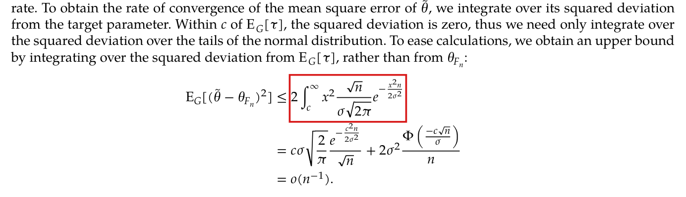
In the proof of Corollary 1, the probability Pr⁡(∣θ^−EG[τ]∣≤c)\Pr(|\hat\theta-\mathrm{E}_G[\tau]|\le c) is 11 and not 00; in the proof of Proposition 4, the Gaussian integral lacks its differential dxdx.

Sentence after Corollary 1, PDF p. 2 (“A proof of Corollary 1 follows by noting that …”); first line of the display in the proof of Proposition 4, PDF p. 3

See also under Formal statements (Lean): P017-T10, P017-T11

As printed

After Corollary 1, PDF p. 2. A proof of Corollary 1 follows by noting that Pr⁡(∣θ^−EG[τ]∣≤c)=0\Pr(|\hat\theta-\mathrm{E}_G[\tau]|\le c)=\colorbox{#ffe58a}{$0$}, and applying Definition 2.

Proof of Proposition 4, PDF p. 3, first line of the display. No differential is printed.

EG[(θ~−θFn)2]≤2∫c∞x2nσ2πe−x2n2σ2\mathrm{E}_G[(\tilde\theta-\theta_{F_n})^2]\le2\int_c^\infty x^2\frac{\sqrt n}{\sigma\sqrt{2\pi}}e^{-\frac{x^2n}{2\sigma^2}}
The problem

The hypothesis of Corollary 1 places the support of θ^\hat\theta inside the interval [EG[τ]−c, EG[τ]+c][\mathrm{E}_G[\tau]-c,\ \mathrm{E}_G[\tau]+c], so that the event ∣θ^−EG[τ]∣≤c|\hat\theta-\mathrm{E}_G[\tau]|\le c has probability one. The proof sentence assigns it probability zero, which contradicts the corollary and the sentence that follows the proof. In the proof of Proposition 4, the integral is printed without dxdx. Both are misprints. In the same display the expectation carries a subscript GG that the statement of Proposition 4 and the sentence after the display omit. This is a difference of notation and not an error, since the sampling expectation is the one induced by GG.

Evidence a derivation

The evidence is a check of the page and a derivation. Let μ=EG[τ]\mu=\mathrm{E}_G[\tau]. The hypothesis c≥max⁡(sup⁡(Supp⁡[θ^])−μ, μ−inf⁡(Supp⁡[θ^]))c\ge\max(\sup(\operatorname{Supp}[\hat\theta])-\mu,\ \mu-\inf(\operatorname{Supp}[\hat\theta])) implies that inf⁡(Supp⁡[θ^])≥μ−c\inf(\operatorname{Supp}[\hat\theta])\ge\mu-c and sup⁡(Supp⁡[θ^])≤μ+c\sup(\operatorname{Supp}[\hat\theta])\le\mu+c. Then ∣θ^−μ∣≤c|\hat\theta-\mu|\le c almost surely, and by Definition 2, I have Pr⁡(θ^=θFn)=1\Pr(\hat\theta=\theta_{F_n})=1. For the integral, set s=σ/ns=\sigma/\sqrt n and a=c/sa=c/s, and let ϕ\phi be the standard normal density. Substituting x=szx=sz and integrating by parts, I obtain

2∫c∞x2nσ2πe−x2n2σ2 dx=2s2∫a∞z2ϕ(z) dz=2s2(aϕ(a)+Φ(−a)),2\int_c^\infty x^2\frac{\sqrt n}{\sigma\sqrt{2\pi}}e^{-\frac{x^2n}{2\sigma^2}}\,dx=2s^2\int_a^\infty z^2\phi(z)\,dz=2s^2\bigl(a\phi(a)+\Phi(-a)\bigr),

which is the second line of the printed display. Numerical integration agrees with the printed closed form at three choices of cc, σ\sigma and nn.

What survives

Corollary 1 and the closed-form evaluation of the integral are correct as printed, and no result changes. The inequality in which the integral appears is a separate matter, treated in P017-E002.

Corrected

A proof of Corollary 1 follows by noting that Pr⁡(∣θ^−EG[τ]∣≤c)=1\Pr(|\hat\theta-\mathrm{E}_G[\tau]|\le c)=\colorbox{#ffe58a}{$1$}, and applying Definition 2.

Proof of Proposition 4, the integral in the first line of the display.

2∫c∞x2nσ2πe−x2n2σ2 dx2\int_c^\infty x^2\frac{\sqrt n}{\sigma\sqrt{2\pi}}e^{-\frac{x^2n}{2\sigma^2}}\colorbox{#ffe58a}{$\displaystyle \,dx$}
Corollary 1, which ends 'Then Pr(theta-hat = theta_Fn) = 1', followed by three lines that begin 'A proof of Corollary 1 follows by noting that Pr(|theta-hat minus E_G[tau]| is at most c) = 0, and applying Definition 2'. A red box marks '= 0'.
Corollary 1 and the first lines of the paragraph that follows it, PDF p. 2. The mark shows the value 00 printed for Pr⁡(∣θ^−EG[τ]∣≤c)\Pr(|\hat\theta-\mathrm{E}_G[\tau]|\le c).
Four lines of the proof of Proposition 4, followed by a display of three lines. A red box marks the integral on the right of the first line of the display, '2 times the integral from c to infinity of x squared times root n over sigma root 2 pi times e to the power minus x squared n over 2 sigma squared'. No dx follows the integrand.
Proof of Proposition 4, PDF p. 3: the four lines before the display, and the display. The marked integral is printed without a differential.

Under the assumptions of Proposition 3, the probability that θ^\hat\theta equals its target tends to one, but at no particular rate; the word “quickly” should be deleted.

Paragraph after the proof of Proposition 3, PDF p. 2, first sentence, the word “quickly”

See also under Formal statements (Lean): P017-T12, P017-T13

As printed

In short, Proposition 3 demonstrates that the probability that θ^\hat\theta falls inside the support of the effect distribution converges to one quickly; conditional on this event, then estimation error is zero (as the target parameter takes on the value as the estimator with probability one).

The problem

The sentence follows a proof in which the expression 2Φ(−cn/σ)2\Phi(-c\sqrt n/\sigma) appears, and in that context “quickly” says that the probability of zero estimation error tends to one at a fast rate. No rate follows from the assumptions of Proposition 3. Definition 1 requires only that n(θ^−EG[τ])=N(0,σ2)+op(1)\sqrt n(\hat\theta-\mathrm{E}_G[\tau])=N(0,\sigma^2)+o_p(1), and the op(1)o_p(1) term may be large on an event whose probability tends to zero arbitrarily slowly. For a decomposition θ^=θ~+u\hat\theta=\tilde\theta+u with θ~=N(EG[τ],σ2/n)\tilde\theta=N(\mathrm{E}_G[\tau],\sigma^2/n), by the union bound, I have

Pr⁡(∣θ^−EG[τ]∣>c)≤2Φ(−cn2σ)+Pr⁡(∣u∣>c/2),\Pr\left(|\hat\theta-\mathrm{E}_G[\tau]|>c\right)\le2\Phi\left(-\frac{c\sqrt n}{2\sigma}\right)+\Pr\left(|u|>c/2\right),

and the condition u=op(n−1/2)u=o_p(n^{-1/2}) does not control the rate of the second term. The sentence prints no specific rate. If “quickly” is read as meaning only that the probability tends to one, then the sentence asserts no rate and needs no correction.

Evidence an exact counterexample

The evidence is an exact counterexample. Let (pn)(p_n) be any sequence in (0,1](0,1] that tends to zero. Let the effect τ\tau equal −1-1 or 11 with probability 1/41/4 each and be uniform on [−1,1][-1,1] otherwise, so that EG[τ]=0\mathrm{E}_G[\tau]=0, the support of τ\tau is [−1,1][-1,1] and c=1c=1. Let the data contain independent observations Xi∼N(0,1)X_i\sim N(0,1) and UiU_i uniform on [0,1)[0,1). Let BnB_n be the indicator of the event that the fractional part of ∑i=1nUi\sum_{i=1}^nU_i is less than pnp_n. I have Pr⁡(Bn=1)=pn\Pr(B_n=1)=p_n, and BnB_n is independent of Xˉn\bar X_n. Let

An=max⁡{−1/2,min⁡(Xˉn,1/2)},θ^=An+10Bn.A_n=\max\{-1/2,\min(\bar X_n,1/2)\},\qquad\hat\theta=A_n+10B_n.

The estimator θ^\hat\theta is a symmetric function of the sample. I have n θ^=n Xˉn+εn\sqrt n\,\hat\theta=\sqrt n\,\bar X_n+\varepsilon_n, where n Xˉn∼N(0,1)\sqrt n\,\bar X_n\sim N(0,1) and Pr⁡(εn≠0)≤4/n+pn→0\Pr(\varepsilon_n\ne0)\le4/n+p_n\to0, and Definition 1 holds with σ2=1\sigma^2=1. If Bn=0B_n=0, then θ^=An∈[−1/2,1/2]\hat\theta=A_n\in[-1/2,1/2] and θFn=θ^\theta_{F_n}=\hat\theta. If Bn=1B_n=1, then θ^≥19/2\hat\theta\ge19/2, θFn=1\theta_{F_n}=1 and the error is at least 17/217/2. I conclude that

Pr⁡(θ^≠θFn)=Pr⁡(∣θ^∣>1)=pn.\Pr(\hat\theta\ne\theta_{F_n})=\Pr(|\hat\theta|>1)=p_n.

For pn=1/(1+⌊log⁡2n⌋)p_n=1/(1+\lfloor\log_2n\rfloor), this probability is 1/101/10 at n=1000n=1000 and 1/401/40 at n=1012n=10^{12}, and it is not O(n−α)O(n^{-\alpha}) for any α>0\alpha>0. The conclusion of Proposition 3 holds in the example, since Pr⁡(n∣θ^−θFn∣>δ)≤pn\Pr(\sqrt n|\hat\theta-\theta_{F_n}|>\delta)\le p_n for all δ>0\delta>0.

What survives

Proposition 3 is unaffected: its conclusion uses only that the probability of the event ∣θ^−EG[τ]∣≤c|\hat\theta-\mathrm{E}_G[\tau]|\le c tends to one. No later result uses a rate for this probability. Proposition 4 makes its own stronger assumption on the remainder, and its conclusion holds under that assumption; the example above does not satisfy it.

Corrected

In short, Proposition 3 demonstrates that the probability that θ^\hat\theta falls inside the interval [EG[τ]−c, EG[τ]+c][\mathrm{E}_G[\tau]-c,\ \mathrm{E}_G[\tau]+c] converges to one quickly; on this event, estimation error is zero (as the target parameter takes on the same value as the estimator with probability one).

In precise terms: if Assumption 1 holds and θ^\hat\theta is a root-nn consistent and asymptotically normal estimator of EG[τ]\mathrm{E}_G[\tau], then Pr⁡(∣θ^−EG[τ]∣≤c)→1\Pr(|\hat\theta-\mathrm{E}_G[\tau]|\le c)\to1, and on this event θ^=θFn\hat\theta=\theta_{F_n}. No rate of convergence of this probability follows from these assumptions. The interval wording is explained in P017-E003.

Three lines of text that begin 'In short, Proposition 3 demonstrates that the probability that theta-hat falls inside the support of the effect distribution converges to one quickly; conditional on this event, then estimation error is zero'. A red box marks the word 'quickly'.
Paragraph after the proof of Proposition 3, PDF p. 2, first three lines. The marked word attributes a fast rate to the probability that the estimation error is zero.

Reference 10 is Working Paper 314 of the U.C. Berkeley Division of Biostatistics Working Paper Series, published in Berkeley, CA, and not in Princeton, NJ; reference 1 lacks its volume, issue and pages, which are 96(1):187–199.

References 1 (PDF p. 3) and 10 (PDF p. 4)

As printed

1. Crump RK, Hotz VJ, Imbens GW, Mitnik OA. Dealing with limited overlap in estimation of average treatment effects. Biometrika 2009.

10. van der Laan MJ, Hubbard AE, Pajouh SK. Statistical inference for data adaptive target parameters. Princeton, NJ: Bepress, 2013.

The problem

Reference 10 names Princeton, NJ as the place of publication. The item is Working Paper 314 of the U.C. Berkeley Division of Biostatistics Working Paper Series, dated June 2013, and its place of publication is Berkeley, CA. Reference 1 has the journal and the year only, although Section 3 cites its p. 188. Both entries still identify the works, and no result depends on them.

Evidence a check of the printed page

The evidence is a check of the page against public bibliographic sources. The page of the series for the working paper (https://biostats.bepress.com/ucbbiostat/paper314/) reads “U.C. Berkeley Division of Biostatistics Working Paper Series. Working Paper 314”, with the date June 2013. A later article by Balzer, Petersen and van der Laan cites the same report as “Berkeley: Division of Biostatistics, University of California; 2013”. The publisher’s page for the article of Crump, Hotz, Imbens and Mitnik has Biometrika 96(1):187–199, 2009. The words quoted in Section 3 appear on p. 188 in the indexed text of a copy in the journal’s format that one of the authors has posted. I did not obtain the working paper itself or the publisher’s full text of the article. The sources do not show at what stage the place of publication was misprinted.

What survives

The discussion and the results are unaffected. The year 2009, the citation of p. 188 and the quotation in Section 3 are correct as printed.

Corrected

1. Crump RK, Hotz VJ, Imbens GW, Mitnik OA. Dealing with limited overlap in estimation of average treatment effects. Biometrika 2009;96(1):187–199.

10. van der Laan MJ, Hubbard AE, Pajouh SK. Statistical inference for data adaptive target parameters. U.C. Berkeley Division of Biostatistics Working Paper Series, Working Paper 314. Berkeley, CA: Bepress, 2013.

Two entries of the reference list. Entry 9 reads 'Balzer LB, Petersen ML, van der Laan MJ. Targeted estimation and inference for the sample average treatment effect Bepress, 2015 Berkeley, CA.' Entry 10 reads 'van der Laan MJ, Hubbard AE, Pajouh SK. Statistical inference for data adaptive target parameters. Princeton, NJ: Bepress, 2013.' A red box marks 'Princeton, NJ'.
References 9 and 10, PDF p. 4. The mark shows the place of publication printed for reference 10. Reference 9, also from Bepress, has Berkeley, CA.
The first entry of the reference list, 'Crump RK, Hotz VJ, Imbens GW, Mitnik OA. Dealing with limited overlap in estimation of average treatment effects. Biometrika 2009.', and the first line of the second entry. A red box marks 'Biometrika 2009.'
Reference 1, PDF p. 3. The marked words are all that the entry prints after the title: the journal and the year, with no volume, issue or pages.

Clarity notes

Imprecise or ambiguous wording whose intended meaning is correct; not an error.

The event on which the estimation error is zero is that θ^\hat\theta lies in the interval [EG[τ]−c, EG[τ]+c][\mathrm{E}_G[\tau]-c,\ \mathrm{E}_G[\tau]+c] of Definition 2, which is not in general the support of the effect distribution.

Paragraph after the proof of Proposition 3, PDF p. 2, first sentence (“In short, Proposition 3 demonstrates …”)

See also under Formal statements (Lean): P017-T13

As printed

In short, Proposition 3 demonstrates that the probability that θ^\hat\theta falls inside the support of the effect distribution converges to one quickly; conditional on this event, then estimation error is zero (as the target parameter takes on the value as the estimator with probability one).

Intended meaning

By Definition 2, θ^=θFn\hat\theta=\theta_{F_n} exactly when ∣θ^−EG[τ]∣≤c|\hat\theta-\mathrm{E}_G[\tau]|\le c. This is the event that the sentence intends: the sentence after the proof of Corollary 1 names the interval [EG[τ]−c, EG[τ]+c][\mathrm{E}_G[\tau]-c,\ \mathrm{E}_G[\tau]+c]. The support of τ\tau is a different set in general. If τ\tau is exponential with mean 11, then the support is [0,∞)[0,\infty) and the interval is [0,2][0,2], and an estimate θ^=3\hat\theta=3 lies in the support with error 11. If τ\tau equals −1-1 or 11 with probability 1/21/2 each, then the interval is [−1,1][-1,1], and an estimate θ^=0.03\hat\theta=0.03 has error zero and lies outside the support {−1,1}\{-1,1\}. With the interval in place of the support, the sentence names the correct event, and since θ^\hat\theta is consistent and c>0c>0, the probability of this event tends to one. No result depends on the sentence.

Corrected

In short, Proposition 3 demonstrates that the probability that θ^\hat\theta falls inside the interval [EG[τ]−c, EG[τ]+c][\mathrm{E}_G[\tau]-c,\ \mathrm{E}_G[\tau]+c] converges to one quickly; on this event, estimation error is zero (as the target parameter takes on the same value as the estimator with probability one).

The deletion of “quickly” is explained in P017-N001.

The last two lines of the proof of Proposition 3, followed by a paragraph of five lines that begins 'In short, Proposition 3 demonstrates that the probability that theta-hat falls inside the support of the effect distribution converges to one quickly'. A red box marks the words 'inside the support of the effect distribution', which run over a line break.
End of the proof of Proposition 3 and the paragraph that follows it, PDF p. 2. The marked words name the support of the effect distribution as the region in which the estimation error is zero.

Formal statements (Lean)

Formal results: 13 whole; 0 restricted; 3 refuted; 0 omitted.

Coverage concerns the identified claim under its stated assumptions. A checked proof establishes the formal statement; correspondence to the published text was reviewed by AI. Repository access is currently required to open the source links.

Each result links to its current formal statement and proof. “Whole” covers the identified claim under its assumptions; “restricted” covers the stated narrower scope; “refuted” gives a counterexample to the identified assertion; “omitted” has no current theorem. Any named published theorem used as a premise remains an assumption. Browse the formal results for this work.

Proposition 1 and the fact cited as its proof, as printed (the witness is the validator’s construction and is not in the paper)

PDF p. 2 (no page number is printed); Assumption 1 on PDF p. 1

Proposition 1 and its proof fact, PDF p. 2; Assumption 1, PDF p. 1. The uniform-effect IID inverse-probability estimator is asymptotically normal and has positive-probability realizations clipping to either unattainable endpoint.

Historical component credits
  • Proved AronowAudit.P017.Wave1.uniform_ipw_counterexample_proof Historical support retained; baseline fidelity: ok; manifest: used; used in Solution; Witness for the printed Proposition 1 and its cited support-interval fact; all T1(a)–(f) components are exported. The strict effect interval ensures endpoint failure is substantive, not a zero-denominator or nonintegrability artifact.
  • Proved AronowAudit.P017.unattainable_upper_endpoint Historical support retained; baseline fidelity: ok; manifest: used; used in Solution; Its component is supplied by the selected composite declaration; no separate application is needed.
  • Proved AronowAudit.P017.ipw_bad_event_probability Historical support retained; baseline fidelity: ok; manifest: used; used in Solution; Its component is supplied by the selected composite declaration; no separate application is needed.
  • Proved AronowAudit.P017.ipw_bad_event_estimator Historical support retained; baseline fidelity: ok; manifest: used; used in Solution; Its component is supplied by the selected composite declaration; no separate application is needed.
  • Proved AronowAudit.P017.ipw_bad_events_disjoint Historical support retained; baseline fidelity: ok; manifest: used; used in Solution; Its component is supplied by the selected composite declaration; no separate application is needed.

The fact cited as the proof of Proposition 1, as corrected (which values a nonnegatively weighted mean attains)

PDF p. 2 (no page number is printed)

the fact cited after Proposition 1, PDF p. 2, corrected. An admissible weighted mean is attainable exactly at an atom or between positive masses on both sides, with all interior, endpoint and exterior support consequences. The prescribed normalized atom indicator and two-region mixture are bounded, nonnegative, admissible, and have weight mean one and weighted-effect mean equal to the target; the conditional means straddle the target and the specified mixing coefficient is strictly between zero and one.

Historical component credits
  • Proved AronowAudit.P017.weighted_mean_characterization Historical support retained; baseline fidelity: ok; manifest: used; used in Solution; Judged against the characterization component identified by row_says. Explicit construction certificates are separately credited to R118-06 and R118-09; their omissions affect target-wide coverage, not the fidelity of this equivalence.
  • Proved AronowAudit.P017.atom_weight_representation Limited support; baseline fidelity: narrower; manifest: used; used in Solution; {'source': 'adjudication+second review', 'adjudicator': 'P017/P017_Audit.lean:362 concludes only that some admissible weight has integral one and weighted mean t. The atom-construction component of T2 explicitly specifies w = 1{τ=t}/Pr_G(τ=t) and says that this weight is bounded. Neither AdmissibleWeight (lines 66–69) nor the existential conclusion identifies that weight or imposes boundedness, so the stated construction is not certified by this declaration. Dropping global integrability of τ is a harmless generalization for this component.', 'suggested_fix': 'Specify w(ω) = if τ(ω) = t then 1 / pr G {ω | τ(ω) = t} else 0 in the conclusion, and assert its admissibility, integral one and weighted mean t; the formula also gives the explicit bound 0 ≤ w(ω) ≤ 1 / pr G {ω | τ(ω) = t}.', 'second_review': "P017/P017_Audit.lean:362 concludes existence of some admissible weight with integral one and weighted mean t, while AdmissibleWeight at P017/P017_Audit.lean:66 imposes neither boundedness nor a particular formula. T2's explicit atom construction requires w = 1{τ=t}/Pr_G(τ=t) and states that this weight is bounded, so the missing construction belongs to the target claim itself. An arbitrary normalized admissible witness need not be that indicator or even be bounded, making this a substantive missing conclusion that requires exporting the formula and its properties. Omitting global integrability of τ is a harmless generalization for this atom subcase.", 'severity': 'major'}
  • Proved AronowAudit.P017.strictly_one_sided_not_representable Historical support retained; baseline fidelity: ok; manifest: used; used in Solution; Its component is supplied by the selected composite declaration; no separate application is needed.
  • Proved AronowAudit.P017.straddling_weight_representation Limited support; baseline fidelity: narrower; manifest: used; used in Solution; Bare interior existence is supplied by the characterization; this row does not certify the prescribed bounded mixture.
  • Proved AronowAudit.P017.support_interior_straddles Historical support retained; baseline fidelity: ok; manifest: used; used in Solution; Its component is supplied by the selected composite declaration; no separate application is needed.
  • Proved AronowAudit.P017.positive_event_meets_support Historical support retained; baseline fidelity: ok; manifest: used; used in Solution; Its component is supplied by the selected composite declaration; no separate application is needed.
  • Proved AronowAudit.P017.representable_support_bounds Historical support retained; baseline fidelity: ok; manifest: used; used in Solution; Its component is supplied by the selected composite declaration; no separate application is needed.
  • Proved AronowAudit.P017.weighted_support_consequences Historical support retained; baseline fidelity: ok; manifest: used; used in Solution; These are exactly the corrected support consequences. Singleton support and infinite support bounds are handled by the real/extended-real quantifiers.

Proposition 1, as corrected with Definition 2 unchanged (the representation holds except at a support endpoint without mass, hence with probability tending to one)

PDF p. 2 (no page number is printed)

Proposition 1 and its gloss, PDF p. 2, corrected. The original clipped target is representable exactly when strictly between the effect-support bounds or at a support endpoint with positive mass. A strictly inside estimate equals its target and satisfies the full chain of clipping and support bounds. Infinite radius, atoms at binding clipping endpoints, and almost surely finite-valued effects give representation on every realization. Under root-n asymptotic normality, both the strictly inside and representation probabilities tend to one.

Historical component credits
  • Proved AronowAudit.P017.Wave1.corrected_proposition1_proof Historical support retained; baseline fidelity: ok; manifest: used; used in Solution; Credit is for the corrected T3, not a proof of the printed all-realizations T9. Measurability is the ordinary random-variable requirement, not an additional moment or support restriction.

Definition 2 and Proposition 1, as corrected to keep the representation in every realization (a fixed clipping radius 0<d<c0 < d < c)

PDF p. 2 (no page number is printed)

Proposition 1 and Definition 2, PDF p. 2, corrected. A positive finite radius smaller than the population radius always exists and makes every clipped estimate representable, with the repaired finite companions and support corollary and the obstruction to substituting a larger radius.

Historical component credits
  • Proved AronowAudit.P017.interior_radius_representation Historical support retained; baseline fidelity: ok; manifest: used; used in Solution; The fixed smaller radius precedes all real estimate values. Both finite and infinite original radius are allowed, and no estimator consistency is assumed.
  • Proved AronowAudit.P017.interior_radius_support Historical support retained; baseline fidelity: ok; manifest: used; used in Solution; Its component is supplied by the selected composite declaration; no separate application is needed.
  • Proved AronowAudit.P017.interior_radius_finite_companions Historical support retained; baseline fidelity: ok; manifest: used; used in Solution; General finite companions, without any asymptotic claim. The outer-probability extension agrees with ordinary sampling probabilities for all intended measurable estimators.
  • Proved AronowAudit.P017.smaller_radius_changes_target Historical support retained; baseline fidelity: ok; manifest: used; used in Solution; Only a pointwise witness is credited here; a constant estimator at the exported x gives failure of radius-d identity under the old radius-c support bound. No root-n-normal estimator counterexample is claimed by this row.
  • Proved AronowAudit.P017.interior_radius_corollary Historical support retained; baseline fidelity: ok; manifest: used; used in Solution; General finite support corollary; specializing μ to the effect mean and 0<d<c gives the repaired-target result. It uses the estimator-law support as required.

Proof of Proposition 3, as printed: the equality Pr⁡(θ~−θFn≠0)=2Φ(−cn/σ)\Pr(\tilde\theta - \theta_{F_n} \ne 0) = 2\Phi(-c\sqrt{n}/\sigma) and the claim that (θ~−θFn)(\tilde\theta - \theta_{F_n}) is op(an)o_p(a_n) for any positive sequence (the witness is the validator’s construction and is not in the paper)

PDF p. 2 (no page number is printed)

proof of Proposition 3, PDF p. 2. The shifted normal sample mean has nonzero intermediate error with probability one and violates the printed every-positive-sequence assertion, while its actual clipping error vanishes on the stated central event.

Historical component credits
  • Proved AronowAudit.P017.Wave1.normal_shift_probability_counterexample_proof Historical support retained; baseline fidelity: ok; manifest: used; used in Solution; The witness refutes the two identified steps concerning tilde minus the actual target, rather than Proposition 3 or the all-rate behavior of the actual clipping error; its sample mean is a statistic of the observed empirical X distribution.
  • Proved AronowAudit.P017.shifted_clip_zero_iff Historical support retained; baseline fidelity: ok; manifest: used; used in Solution; Its component is supplied by the selected composite declaration; no separate application is needed.

Proof of Proposition 4, as printed: “Within cc of EG[τ]\mathrm{E}_G[\tau], the squared deviation is zero” and the first inequality of the display (the witness is the validator’s construction and is not in the paper)

PDF p. 3 (no page number is printed)

proof of Proposition 4, PDF p. 3. The shifted normal estimator satisfies the remainder condition but at size 25 has positive central intermediate error and a mean-square gap above the printed tail bound, while both true mean-square limits still hold.

Historical component credits
  • Proved AronowAudit.P017.Wave1.normal_shift_mse_counterexample_proof Historical support retained; baseline fidelity: ok; manifest: used; used in Solution; The model satisfies the printed Proposition 4 decomposition and moment condition. The 6/15625 positive gap concerns the intermediate difference, and does not contradict the proposition's MSE limit.
  • Proved AronowAudit.P017.shifted_25_central Historical support retained; baseline fidelity: ok; manifest: used; used in Solution; This row exports the scalar ranges and central-event algebra only; R119-03 supplies the probability and expectation certificates.
  • Proved AronowAudit.P017.normal_shift_remainder_ms Historical support retained; baseline fidelity: ok; manifest: used; used in Solution; Its component is supplied by the selected composite declaration; no separate application is needed.

Proof of Proposition 3, as repaired (the clipping-event bound for the actual estimator; the every-positive-sequence rate for θ^−θFn\hat\theta - \theta_{F_n})

PDF p. 2 (no page number is printed)

proof of Proposition 3, PDF p. 2, corrected. With the finite population mean and positive, possibly infinite effect radius of Assumption 1, the actual clipping error has its exact zero region and exceedance-event inclusion and probability bound at every positive sample size. Consistency alone gives every fixed-radius tail limit, the clipping-failure probability limit, o_p(a_n) actual error for every deterministic sequence positive at n ≥ 1, and root-n actual error o_p(1). Definition 1 additionally gives root-n boundedness in probability and consistency, hence all these limits. At infinite radius the target is the estimate and both the actual error and its root-n scaling are identically zero. The clipping-event deduction requires no normal decomposition or rate for the clipping-failure probability. The usual measure-theoretic conditions are assumed.

Historical component credits
  • Proved AronowAudit.P017.corrected_proposition3 Historical support retained; baseline fidelity: ok; manifest: not used; not used in Solution; The population integrability and measurability are the finite-mean random-effect assumptions, and RootNNormal is the packet's accepted distributional reading. Metadata issue: T7's final sentence says all of (a)–(c) use only consistency, but the root-n tightness assertion within (b) needs the stronger root-n assumption; the Lean correctly retains it.
  • Proved AronowAudit.P017.clipReal_bounds Historical support retained; baseline fidelity: ok; manifest: used; used in Solution; Its component is supplied by the selected composite declaration; no separate application is needed.
  • Proved AronowAudit.P017.clipReal_eq_self_iff Historical support retained; baseline fidelity: ok; manifest: used; used in Solution; Its component is supplied by the selected composite declaration; no separate application is needed.
  • Proved AronowAudit.P017.clipTarget_eq_self_iff Historical support retained; baseline fidelity: ok; manifest: used; used in Solution; The generalization loses no target cases and changes none of its positive-radius specializations.
  • Proved AronowAudit.P017.consistent_clipping_all_rates Historical support retained; baseline fidelity: ok; manifest: not used; not used in Solution; Its component is supplied by the selected composite declaration; no separate application is needed.
  • Proved AronowAudit.P017.root_normal_tight_and_consistent Historical support retained; baseline fidelity: ok; manifest: used; used in Solution; No tightness or consistency result is assumed as an extra premise: both are conclusions. The target's claim that consistency alone suffices should not be read as asserting root-n tightness from consistency.
  • Proved AronowAudit.P017.clipping_event_bound Limited support; baseline fidelity: narrower; manifest: not used; not used in Solution; Use the credited equality characterization and measure monotonicity to state the inclusion and probability bound for extended radius.
  • Proved AronowAudit.P017.consistency_event_bound Historical support retained; baseline fidelity: ok; manifest: used; used in Solution; Its component is supplied by the selected composite declaration; no separate application is needed.

Proof of Proposition 4, as repaired (the clipping residual is 1-Lipschitz; a mean-square bound for the actual estimator)

PDF p. 3 (no page number is printed)

proof of Proposition 4, PDF p. 3, corrected. The Lipschitz clipping and residual inequalities give the finite Gaussian fourth-moment bounds, both mean-square limits, and zero actual error at infinite radius. The usual measure-theoretic conditions are assumed.

Historical component credits
  • Proved AronowAudit.P017.Wave1.corrected_proposition4_finite_proof Historical support retained; baseline fidelity: ok; manifest: used; used in Solution; Every finite certificate in the assigned component is exported, including both squared-error bounds, the fourth moment, the residual positive-part identity and the correctly attributed auxiliary tail identity. R119-15 and R119-17 are responsible for the limit and infinite-radius components.
  • Proved AronowAudit.P017.Wave1.corrected_proposition4_limits_proof Historical support retained; baseline fidelity: ok; manifest: used; used in Solution; The finite-second-moment and normal-remainder hypotheses are those in T8's full corrected argument, with ordinary measurability of random variables. They imply integrability of the squared errors at every n≥1, so the limits do not exploit the zero value of an undefined Bochner integral.
  • Proved AronowAudit.P017.ordered_clip_changes Historical support retained; baseline fidelity: ok; manifest: used; used in Solution; Its component is supplied by the selected composite declaration; no separate application is needed.
  • Proved AronowAudit.P017.clip_and_residual_lipschitz Historical support retained; baseline fidelity: ok; manifest: used; used in Solution; Its component is supplied by the selected composite declaration; no separate application is needed.
  • Proved AronowAudit.P017.residual_tail_fourth_bound Historical support retained; baseline fidelity: ok; manifest: used; used in Solution; Its component is supplied by the selected composite declaration; no separate application is needed.
  • Proved AronowAudit.P017.perturbation_square_bounds Historical support retained; baseline fidelity: ok; manifest: used; used in Solution; Its component is supplied by the selected composite declaration; no separate application is needed.
  • Proved AronowAudit.P017.infinite_radius_facts Historical support retained; baseline fidelity: ok; manifest: used; used in Solution; Metadata wording issue: the quoted correction says both errors are identically zero at infinity, but the detailed T8 statement correctly asserts only zero actual MSE. The statement preserves the necessary distinction; a literal reading that the normal-to-actual-target difference is also zero would be false.

Proposition 1

PDF p. 2 (no page number is printed)

The printed claim is false: the universal empirical-statistic representation assertion fails even with IID full-data draws from G, measurable observed records and an estimator given by a measurable functional of the observed empirical law, integrable effects, positive radius, and asymptotic normality. The counterexample samples independently from the specified population G; IID sampling supplies a valid counterexample to the printed all-realizations assertion. Proposition 1 and its all-realizations gloss, PDF p. 2. The usual measure-theoretic conditions are assumed.

Historical component credits

Corollary 1, with the probability in its proof sentence corrected from 0 to 1

PDF p. 2 (no page number is printed)

Corollary 1, its proof, and its two support remarks, PDF p. 2, corrected. Estimator support inside the clipping interval gives probability one of zero error; full real effect support gives the identity target, while nonnegative effect support and negative estimates give the stated strict loss of equality probability. The usual measure-theoretic conditions are assumed.

Historical component credits
  • Proved AronowAudit.P017.corollary1_corrected Historical support retained; baseline fidelity: ok; manifest: used; used in Solution; The final zero-probability implication has an impossible antecedent under hcond, already recognized in the blind backtranslation; the independently exported exact event equality supplies the meaningful implication in T10(c). The theorem as a whole has nondegenerate instances.
  • Proved AronowAudit.P017.full_real_support Historical support retained; baseline fidelity: ok; manifest: used; used in Solution; The maximum-support condition is automatically true once c=+∞, so its omission as a separate conjunct loses no content. Population integrability is part of the standing assumptions even though the clipping identity itself does not need it.
  • Proved AronowAudit.P017.positive_support_negative_estimates Historical support retained; baseline fidelity: ok; manifest: used; used in Solution; {'source': 'adjudication', 'decision': 'rejected', 'what': 'At AronowAudit/P017/P017_Audit.lean:1062, the hypotheses use the actual effect-law support [0,infinity), finite mean, and positive sampling probability of negative estimates. The conclusions give c=mu, failure of the corollary support condition, and Pr(hat=target) <= 1-Pr(hat<0) < 1, exactly matching T10(e). The closed half-line agrees with the standing closed-support reading of the printed R+ notation, and the measurable random-variable hypotheses introduce no material restriction. The reviewer correctly identifies a description error: the shared sentence saying the interval and equality probabilities are one applies under the corollary support condition, which this row proves fails.'}
  • Proved AronowAudit.P017.support_interval_of_condition Historical support retained; baseline fidelity: ok; manifest: used; used in Solution; Its component is supplied by the selected composite declaration; no separate application is needed.
  • Proved AronowAudit.P017.support_interval_probability Limited support; baseline fidelity: narrower; manifest: used; used in Solution; Its component is supplied by the selected composite declaration; no separate application is needed.

Display in the proof of Proposition 4: the normal tail integral, with its differential restored, and its closed form

PDF p. 3 (no page number is printed)

the normal-tail display in the proof of Proposition 4, PDF p. 3, corrected. The displayed Lebesgue tail integral equals its closed form, the truncated second moment of any random variable with the specified Gaussian law, and the scale-s density/CDF expression. The standardized density integral has the stated integration-by-parts value. The relevant integrands are integrable, and the common value decays faster than every positive power of sample size. At infinite radius the tail set is empty, its integral and truncated moment are zero, and the same power limits hold. The usual measure-theoretic conditions are assumed.

Historical component credits
  • Proved AronowAudit.P017.Wave1.normal_tail_identity_proof Historical support retained; baseline fidelity: ok; manifest: used; used in Solution; The corrected target itself restores dx. Using an open Lebesgue half-line rather than a closed endpoint changes nothing because a singleton is null. The false leading MSE inequality in the printed display is outside this row and this corrected identity target.
  • Proved AronowAudit.P017.Wave1.normal_tail_limits_proof Historical support retained; baseline fidelity: ok; manifest: used; used in Solution; All positive real powers are explicitly in the target, so the second conjunct is not an uncredited change of claim. Metadata inconsistency: T11.asymptotic is false although the target and this row contain asymptotic limits.

Sentence after the proof of Proposition 3, “converges to one quickly” (the witness is the validator’s construction and is not in the paper)

PDF p. 2 (no page number is printed)

the sentence after Proposition 3, PDF p. 2. The IID rare-outlier construction realizes every positive vanishing clipping- failure sequence under the stated hypotheses. It is a statistic of the observed empirical distribution and has the stated exact events, normal decomposition, finite moment bounds, central-event probability bounds and probability limits. The logarithmic example has the stated numerical values and slow rates, and fails the mean-square remainder condition. For each prescribed positive vanishing rate r, the explicit sequence min(1, sqrt(r)) equals sqrt(r) eventually, tends to zero, and its ratio to r tends to infinity; the same construction realizes it. These facts refute a universal-rate interpretation of "quickly"; the printed sentence specifies no numerical rate.

Historical component credits
  • Proved AronowAudit.P017.Wave1.slow_outlier_counterexample_proof Historical support retained; baseline fidelity: ok; manifest: used; used in Solution; The witness contradicts any uniform polynomial or Gaussian-speed reading, while the paper never states a numerical bound with quickly; the row accurately disclaims a full formal negation of a printed quantitative theorem. For the concrete logarithmic p, failure of SmallRemainderMS distinguishes it from Proposition 4. Ancillary finite identities are supplied by R120-08, not inferred from a hidden proof.
  • Proved AronowAudit.P017.Wave1.arbitrary_outlier_sequence_proof Historical support retained; baseline fidelity: ok; manifest: used; used in Solution; The row establishes the assigned parametrized witness components, not an assertion that every vanishing p is slow and not a formal negation of the unquantified word quickly. The exact standard-normal law, decomposition and o_P(1) remainder export variance-one asymptotic normality despite RootNNormal itself existentially quantifying its variance. Metadata: T12.asymptotic=false conflicts with its explicit limit assertions.
  • Proved AronowAudit.P017.rare_estimator_finite Historical support retained; baseline fidelity: ok; manifest: used; used in Solution; {'source': 'adjudication', 'decision': 'rejected', 'what': 'At AronowAudit/P017/P017_Audit.lean:1642, A is the clip of x to [-1/2,1/2], equivalent to the max/min expression in the counterexample. The identities clip(A)=A and clip(A+10)=1 give the zero-error and outlier branches of T12(d), with outlier error (A+10)-1=A+9 and exactly the claimed bounds. Quantification over every real x covers every normal input and is sufficient for this identified finite algebra component. The only error is in the modelling paragraph: this declaration fixes center 0 and radii 1/2 and 1, whereas the paragraph incorrectly describes an arbitrary center and an explicit radius hypothesis.'}
  • Proved AronowAudit.P017.slow_probability_numbers Historical support retained; baseline fidelity: ok; manifest: used; used in Solution; Its component is supplied by the selected composite declaration; no separate application is needed.
  • Proved AronowAudit.P017.slow_probability_positive_limit Historical support retained; baseline fidelity: ok; manifest: used; used in Solution; The harmless n=0 value is also covered, with q_0=1; all statistical failure probabilities are asserted only for n≥1.

Sentence after the proof of Proposition 3, as repaired (“quickly” deleted; the event is the interval of Definition 2)

PDF p. 2 (no page number is printed)

the sentence after Proposition 3, PDF p. 2, corrected. The clipping interval is exactly the zero-error event with probability tending to one, every prescribed positive vanishing failure rate is realizable, and a finite normal-plus- remainder probability bound retains the uncontrolled remainder probability. The usual measure-theoretic conditions are assumed.

Historical component credits
  • Proved AronowAudit.P017.corrected_zero_error_sentence Historical support retained; baseline fidelity: ok; manifest: used; used in Solution; The interval is the zero-error region; the theorem does not identify it with possibly disconnected effect support. The separate population and sampling measures and weak convergence match the target standing reading.
  • Proved AronowAudit.P017.Wave1.normal_plus_remainder_failure_bound_proof Historical support retained; baseline fidelity: ok; manifest: used; used in Solution; This is the corrected finite bound T13(d), not the false Gaussian-only formula for an intermediate event in the printed proof. Dependence between the normal part and u is allowed; no convergence rate for the retained remainder term is claimed.
  • Proved AronowAudit.P017.sum_failure_union_bound Historical support retained; baseline fidelity: ok; manifest: used; used in Solution; Its component is supplied by the selected composite declaration; no separate application is needed.
  • Proved AronowAudit.P017.Wave1.arbitrary_outlier_sequence_proof Historical support retained; baseline fidelity: ok; manifest: used; used in Solution; A fixed population with μ=0 and c=1 is sufficient because T13(c) existentially quantifies the law and estimator after each prescribed p. All required failure-event equalities and asymptotic normality are exported by the declaration.

Proposition 3, with its proof as printed

PDF p. 2 (no page number is printed)

The printed claim is false: P017-T14; Proposition 3 and its printed proof, PDF p. 2. In the admissible shifted-normal example the intermediate error from the actual target fails a positive-sequence little-o assertion, and its nonzero probability is one rather than the asserted Gaussian tail. The proposition's actual root-n error conclusion remains valid under all its original assumptions. The usual measure-theoretic conditions are assumed.

Historical component credits
  • Proved AronowAudit.P017.proposition3 Historical support retained; baseline fidelity: ok; manifest: used; used in Solution; RootNNormal is the explicitly authorized weak-convergence reading of Definition 1, not mere consistency. Positive radius is retained and the conclusion uses the actual estimator-dependent target; no false intermediate proof identity is assumed.

Proposition 4, with its proof as printed

PDF p. 3 (no page number is printed); introduced on PDF p. 2, last paragraph

The printed claim is false: P017-T15; Proposition 4 and its printed proof, PDF p. 3. The shifted-normal example satisfies the exact Gaussian-plus-remainder condition and its moment rate, yet has positive intermediate squared error in the central region at size 25 and an intermediate mean-square error strictly above the printed Gaussian-tail bound. The proposition's actual mean-square conclusion remains valid without independence. The usual measure-theoretic conditions are assumed.

Historical component credits
  • Proved AronowAudit.P017.Wave1.proposition4_proof Historical support retained; baseline fidelity: ok; manifest: used; used in Solution; NormalRemainder expands to exact Gaussian marginal laws, square-integrable remainders and almost-sure decomposition for every n≥1, without independence. These hypotheses give genuine finite actual-error second moments, avoiding the integral-zero convention; n=0 does not affect the limit.

Proposition 2

PDF p. 2 (no page number is printed)

Proposition 2 and its pointwise proof, PDF p. 2. The clipped target minus the population mean, multiplied by sqrt(n), is bounded in probability under root-n asymptotic normality, with zero and infinite radius allowed.

Historical component credits
  • Proved AronowAudit.P017.proposition2 Historical support retained; baseline fidelity: ok; manifest: used; used in Solution; RootNNormal is genuine weak convergence with finite positive Gaussian variance; BoundedInProbability has exactly the required ε,M,eventual-n order. Population integrability prevents a zero-by-default integral, measurable pushforwards avoid fallback laws, and the c=0 and c=+∞ cases are included. No claim-stage verdict change.
  • Proved AronowAudit.P017.clipReal_distance Historical support retained; baseline fidelity: ok; manifest: used; used in Solution; Its component is supplied by the selected composite declaration; no separate application is needed.
  • Proved AronowAudit.P017.clipTarget_distance Historical support retained; baseline fidelity: ok; manifest: used; used in Solution; The +∞ branch returns x before any conversion to a real radius, so ENNReal.toReal(+∞)=0 causes no lost case. This supplies the full pointwise auxiliary inequality, not the asymptotic conclusion by itself. No claim-stage verdict change.

Reproduction

What I recalculated or reran from public materials. "Agrees", "Agrees in part" or "Disagrees" compares my result with the printed one. "Not compared" means the comparison could not be made.

Status
Not applicable
Agreement
Not applicable