Journal article P021

Corrections to: Nonparametric Identification for Respondent-Driven Sampling

P. M. Aronow and Forrest W. Crawford (2015). Nonparametric Identification for Respondent-Driven Sampling. Statistics and Probability Letters 106:100–102.

DOI: 10.1016/j.spl.2015.07.003
arXiv: 1504.03574
Audited edition: Statistics and Probability Letters, 2015, 106:100–102; 3 pages in the audited file
SHA-256 of the audited file: bbe090b4e767b80d2cd4189d70e0d65c238b452f78ef925d1c438732b91db484
Permanent address: https://pmaronow.github.io/llm-audit/works/P021/

Summary

This note asks when the Volz–Heckathorn estimator for respondent-driven sampling is consistent. It shows that the population mean is identified when outcomes are mean-ignorable given degree and the sampling probability is positive and is a function of degree known up to scale (Proposition 1), and that the estimator is consistent under the standing convergence and common-bound assumptions when this function is proportional to degree (Corollary 1). 2 entries are classified as errors (2 Minor), both in the reference list, and 2 are clarity notes on how the assumptions are stated. Two possible errors were not confirmed.

What was and was not checked

I checked the following, with the qualifications stated below.

Equation (1) is the inverse-degree ratio estimator of Volz and Heckathorn, and it is the sample version of (2) with $f(k)=k$ .
Proposition 1 and its proof. Equation (3) follows from Bayes' rule and Condition 2. In (4), the law of total expectation is applied correctly, and the unknown scale $\Pr[S=1]/c$ cancels. Both steps hold on the degrees with positive probability (see P021-N003). Exact calculations agree with (2) in 25 examples, on 200 randomly generated joint laws, and symbolically for $K=3$ .
Mean ignorability within each degree class is enough for Proposition 1. Formula (2) holds on laws in which sampling depends on the outcome within a degree class, and formula (2) does not change when $f$ is rescaled.
Corollary 1, under the convergence assumed in the first sentence of Section 2 and bounds common to the sequence (see P021-E001). The derivation does not use independence or the random-walk model.
The comparison with the random-walk model, for the limiting population law and the limiting law of the visit records. These two laws can be represented by a joint law that satisfies Conditions 1 and 2 with $f(k)=k$ . The paper does not define the indicator $S$ when a subject is recruited more than once.
Three remarks of the Discussion. Ignorability given degree alone does not identify the mean, since two models with the same observed law have means $1/2$ and $1/4$ . For a strictly positive $f$ , every observed law of $(Y,D)$ given $S=1$ is compatible with Conditions 1 and 2. Neither condition requires any network-structure assumption of Table 1.
The citations. Each of the 20 works cited in the text has a reference entry, and each of the 20 entries is cited. The quotation from Gile et al. (2015) and the substantive entries of Table 1 agree with that article. The reference entries agree with the publishers' or indexers' records in the checked publication details, apart from the items in P021-E002 and P021-N001.

I could not obtain the body of the final article of Gile (2011). I read its preprint and the publisher’s abstract, which support the citation on p. 100. I compared the other cited works with the note for their publication details only. I did not test on data the remark that the estimator may be appropriate when the diagnostics of Gile et al. (2015) fail; it states a logical possibility. The note has no numerical results, simulations, data or code, and it refers to no appendix or supplement. There were no empirical numerical results to recompute.

Headline claims and related corrections

Mean ignorability within degree classes, with every class sampled with positive probability (Condition 1), together with knowledge of the degree-specific sampling probability up to an unknown scale (Condition 2), nonparametrically identifies the population mean by the normalized inverse-probability formula (2).
Conditions 1 and 2; Proposition 1; Eqs. (2)-(4)
See P021-E001, P021-N003.
Under the convergence setup of Section 2 and Conditions 1 and 2 with $f(k)$ proportional to $k$ , the Volz–Heckathorn estimator (1) is consistent for the population mean.
Corollary 1; Eq. (1); Proposition 1
See P021-E001.
The conditions for consistency of the VH estimator are weaker than previously assumed: they are less stringent than the traditional random-walk model, consistency requires neither random sampling nor an actual network, and neither Condition requires any of the network-structure assumptions of Table 1.
Corollary 1 and Conditions 1-2 set against Table 1
Ignorability given degree alone does not identify the population mean in RDS because the population degree distribution is unknown; specifying the conditional sampling probability up to scale (Condition 2) supplies the missing reweighting, which is the difficulty RDS adds to other non-probability samples.
Conditions 1 and 2; Proposition 1, Eq. (3)
Without information on unsampled subjects neither Condition 1 nor Condition 2 has directly testable implications, so the value of any diagnostic depends on further assumptions about the generative (recruitment) process.
Conditions 1 and 2; Proposition 1; Corollary 1; Table 1
See P021-N003.
The VH estimator and its inverse-probability variants may be appropriate even when diagnostics predicated on a more restrictive network model, such as those of Gile et al. (2015), fail.
Table 1; Proposition 1; Corollary 1

Corrections

Minor (2)

Real but inconsequential, for example a misprint that does not change a result.

P021-E002 Minor

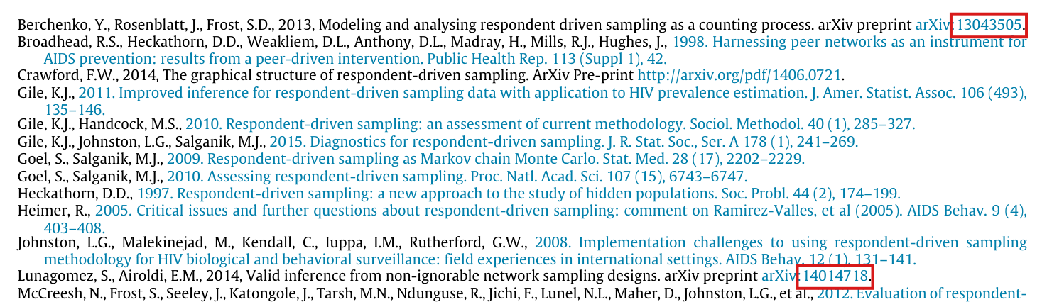
The two arXiv identifiers should read arXiv:1304.3505 and arXiv:1401.4718; each is printed without the dot.

References, p. 102 (PDF p. 3): the entries for Berchenko, Rosenblatt and Frost (2013) and for Lunagomez and Airoldi (2014)

As printed

Berchenko, Y., Rosenblatt, J., Frost, S.D., 2013, Modeling and analysing respondent driven sampling as a counting process. arXiv preprint arXiv:13043505.

Lunagomez, S., Airoldi, E.M., 2014, Valid inference from non-ignorable network sampling designs. arXiv preprint arXiv:14014718.

The problem

An arXiv identifier of 2013 or 2014 has a dot between the four digits of the year and month and the serial number. Both entries print the eight digits without the dot, and the links in the PDF point to the same strings.

Evidence a check of the printed page

I checked the page: both identifiers appear without the dot on p. 102, while the entry for Crawford (2014) on the same page prints 1406.0721 with the dot. In the PDF, the two links point to addresses that end in 13043505 and 14014718. The first versions of arXiv:1304.3505 and arXiv:1401.4718 carry the cited titles and authors.

What survives

No result, proof or estimator depends on these entries. Only the two identifiers and their links change.

Corrected

Berchenko, Y., Rosenblatt, J., Frost, S.D., 2013, Modeling and analysing respondent driven sampling as a counting process. arXiv preprint arXiv:1304.3505.

Lunagomez, S., Airoldi, E.M., 2014, Valid inference from non-ignorable network sampling designs. arXiv preprint arXiv:1401.4718.

The links should point to https://arxiv.org/abs/1304.3505 and https://arxiv.org/abs/1401.4718.

Crop of the reference list, from the entry for Berchenko, Rosenblatt and Frost to the first line of the entry for McCreesh and coauthors. Red outlines surround the digits 13043505 at the end of the Berchenko entry and the digits 14014718 at the end of the entry for Lunagomez and Airoldi. The Crawford entry reads http://arxiv.org/pdf/1406.0721. — References, p. 102 (PDF p. 3). The outlines mark the two arXiv identifiers printed without the dot. The entry for Crawford (2014), three lines below the first, prints its identifier with the dot.

P021-N001 Minor

Two reference entries give a supplement as the ordinary issue 1: the issues are AIDS Behav. 12 (Suppl 1) and J. Urban Health 83 (Suppl 1).

References, p. 102 (PDF p. 3): the entries for Johnston et al. (2008) and for Salganik (2006)

As printed

Johnston, L.G., Malekinejad, M., Kendall, C., Iuppa, I.M., Rutherford, G.W., 2008. Implementation challenges to using respondent-driven sampling methodology for HIV biological and behavioral surveillance: field experiences in international settings. AIDS Behav. 12 (1), 131–141.

Salganik, M.J., 2006. Variance estimation, design effects, and sample size calculations for respondent-driven sampling. J. Urban Health 83 (1), 98–112.

The problem

Both articles appeared in supplements to their volumes, and the two entries print the supplement as the ordinary issue “(1)”. The volumes and the page ranges are correct, and both articles can still be found from them. The two arXiv identifiers in the same list are the subject of P021-E002.

Evidence a check of the printed page

I compared the entries with the publisher’s pages for the two articles. The page for the article of Johnston et al. gives “AIDS Behav 12 (Suppl 1), 131–141 (2008)” (https://link.springer.com/article/10.1007/s10461-008-9413-1). The page for the article of Salganik gives “J Urban Health 83 (Suppl 1), 98–112 (2006)” (https://link.springer.com/article/10.1007/s11524-006-9106-x). The National Library of Medicine indexes the same articles as 12(4 Suppl):S131–S141 and 83(6 Suppl):i98–i112.

What survives

No result depends on these entries. A comparison with the article of Gile et al. (2015) supports the attributions to it. The phrase quoted with the locator “pg. 3” is on the third page of their article, p. 243, and Table 1 keeps every substantive entry of their Table 1 on p. 244. The other entries of the reference list agree with the publishers' or indexers' records in volume, issue, year and first page. The entries for Broadhead et al. (1998) and McCreesh et al. (2012) give only the first page of the ranges 42–57 and 138–147.

Corrected

Salganik, M.J., 2006. Variance estimation, design effects, and sample size calculations for respondent-driven sampling. J. Urban Health 83 (Suppl 1), 98–112.

Crop of nine lines of the reference list, from the entry for Johnston and coauthors to the entry for Salganik (2012). Red outlines surround the volume and issue 12 (1) before the pages 131 to 141 in the Johnston entry, and the volume and issue 83 (1) before the pages 98 to 112 in the entry for Salganik (2006). — References, p. 102 (PDF p. 3). The outlines mark the volume and issue, “12 (1)” and “83 (1)”, in the entries for Johnston et al. (2008) and for Salganik (2006).

Clarity notes

Imprecise or ambiguous wording whose intended meaning is correct; not an error.

P021-E001 Clarity note

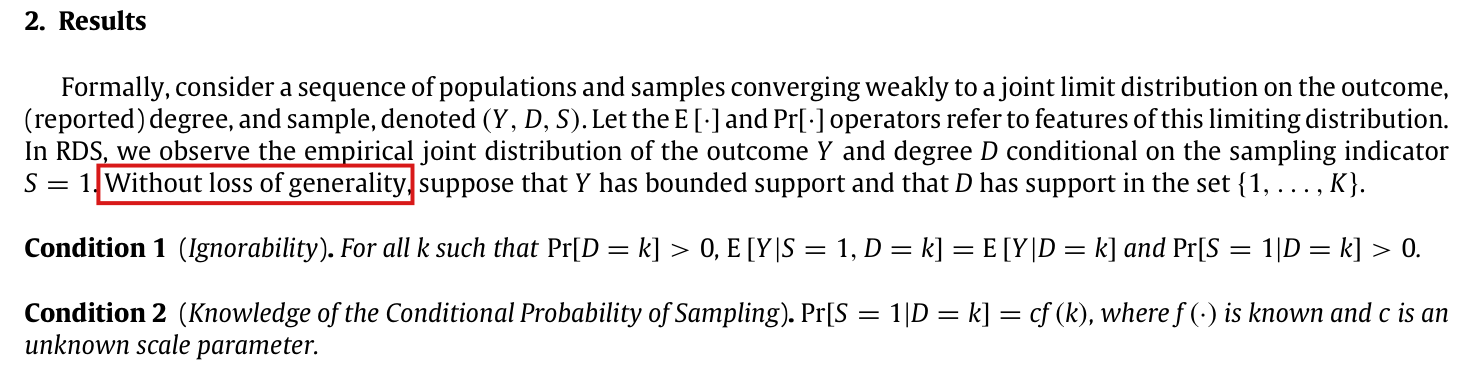
The bounds on the outcome and on the degree are assumptions that hold for every population in the sequence, and they are not made without loss of generality.

Section 2, first paragraph, last sentence, p. 101 (PDF p. 2)

See also under Formal statements (Lean): P021-T2

As printed

Formally, consider a sequence of populations and samples converging weakly to a joint limit distribution on the outcome, (reported) degree, and sample, denoted $(Y, D, S)$ . Let the $\mathrm{E}[\cdot]$ and $\Pr[\cdot]$ operators refer to features of this limiting distribution. In RDS, we observe the empirical joint distribution of the outcome $Y$ and degree $D$ conditional on the sampling indicator $S = 1$ . Without loss of generality, suppose that $Y$ has bounded support and that $D$ has support in the set $\{1, \ldots, K\}$ .

Intended meaning

The two bounds are meant as standing assumptions, made for simplicity. Every population in the sequence has outcomes in a common interval $[-B,B]$ and degrees in $\{1,\ldots,K\}$ . On this reading, Proposition 1 and Corollary 1 are correct. For Corollary 1, suppose that $\Pr[S=1\mid D=k]=ak$ with $a>0$ , and let $A_N$ and $H_N$ denote the averages of $sy/d$ and $s/d$ over the $N$ units of a population, where $s=1$ for a sampled unit and $s=0$ otherwise. The estimator (1) equals $A_N/H_N$ . Since the functions $sy/d$ and $s/d$ are bounded and continuous on $[-B,B]\times\{1,\ldots,K\}\times\{0,1\}$ , the weak convergence assumed in the first sentence of Section 2 implies that

H_N \to \mathrm{E}[S/D] = a, \qquad A_N \to \mathrm{E}[SY/D] = a\,\mathrm{E}[Y],

where I used Condition 1 in the last equality. I conclude that $A_N/H_N \to \mathrm{E}[Y]$ .

The words “without loss of generality” claim more than this, and two exact examples explain the outcome restriction. First, let $D=1$ , let $\Pr[Y=j]=2/3^{j+1}$ for every integer $j\ge 0$ , and let $S$ be independent of $Y$ with $\Pr[S=1]=2/5$ . Then Conditions 1 and 2 hold with $f(1)=1$ and $c=2/5$ , and $\mathrm{E}[Y]=1/2$ . The outcome is unbounded, and clipping $Y$ at an integer $M\ge 1$ changes the mean to $(1-3^{-M})/2$ . Second, a bound on the limiting $Y$ alone is not enough for Corollary 1. For each $m\ge 1$ , I consider a population of $N=3m$ units of degree $1$ in which $m$ units are sampled, one sampled unit has the outcome $2m$ , and every other unit has the outcome $0$ . The empirical joint laws converge weakly to the law with mass $2/3$ at $(Y,D,S)=(0,1,0)$ and mass $1/3$ at $(0,1,1)$ . This limit satisfies Conditions 1 and 2 with $f(1)=1$ and $c=1/3$ , and it has $\mathrm{E}[Y]=0$ . However, $A_N=2/3$ and $H_N=1/3$ , and the estimator (1) equals $2$ for every $m$ .

The common bound on the degree is stronger than Corollary 1 needs. When $\Pr[S=1\mid D=k]=ak$ , the positivity in Condition 1 excludes degree $0$ , and the inequality $ak\le 1$ bounds the degrees of the limit. A condition under which $A_N$ and $H_N$ converge to $\mathrm{E}[SY/D]$ and $\mathrm{E}[S/D]$ can replace the common bound on the outcome.

Corrected

Formally, consider a sequence of populations and samples whose empirical joint laws converge weakly, in probability if they are random, to a joint limit distribution on the outcome, (reported) degree, and sample, denoted $(Y, D, S)$ . Let the $\mathrm{E}[\cdot]$ and $\Pr[\cdot]$ operators refer to features of this limiting distribution. In RDS, we observe the empirical joint distribution of the outcome $Y$ and degree $D$ conditional on the sampling indicator $S = 1$ . For simplicity, assume that there exist constants $B<\infty$ and $K<\infty$ such that every population in the sequence has outcomes in $[-B,B]$ and degrees in $\{1, \ldots, K\}$ .

Crop of the heading 2. Results, the first paragraph of the section, and Conditions 1 and 2. A red outline surrounds the words Without loss of generality at the start of the last sentence of the paragraph. The sentence continues: suppose that Y has bounded support and that D has support in the set 1 to K. — Section 2, first paragraph, p. 101 (PDF p. 2). The outline marks the words “Without loss of generality”, which introduce the bounds on the outcome and on the degree.

P021-N003 Clarity note

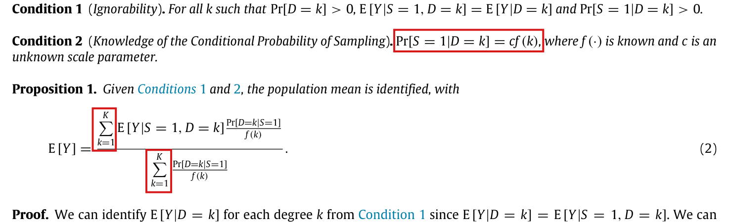
Condition 2 and the sums in (2) and (4) are meant for the degrees $k$ such that $\Pr[D=k]>0$ , the restriction that Condition 1 states.

Condition 2, Proposition 1 with equation (2), and the proof with equations (3) and (4), p. 101 (PDF p. 2); Discussion, second paragraph, p. 102 (PDF p. 3)

See also under Formal statements (Lean): P021-T1

As printed

Section 2, p. 101. Condition 2 (Knowledge of the Conditional Probability of Sampling). $\Pr[S = 1 \mid D = \colorbox{#ffe58a}{$k$}] = cf(k)$ , where $f(\cdot)$ is known and $c$ is an unknown scale parameter.

Proposition 1. Given Conditions 1 and 2, the population mean is identified, with

\mathrm{E}[Y] = \frac{\colorbox{#ffe58a}{$\displaystyle \sum_{k=1}^{K}$} \mathrm{E}[Y \mid S = 1, D = k]\,\frac{\Pr[D = k \mid S = 1]}{f(k)}}{\colorbox{#ffe58a}{$\displaystyle \sum_{k=1}^{K}$} \frac{\Pr[D = k \mid S = 1]}{f(k)}}. \qquad (2)

Discussion, p. 102. Without knowledge of the characteristics of the unsampled subjects, neither Condition 1 nor Condition 2 has directly testable implications, and thus the value of any diagnostics must depend on further assumptions about the generative process.

Intended meaning

Condition 1 is stated for the degrees $k$ such that $\Pr[D=k]>0$ . Condition 2, the proof’s “for each degree $k$ ”, equation (3) and the sums in (2) and (4) are meant for the same degrees, and I write $A=\{k:\Pr[D=k]>0\}$ for this set. Read literally, the sums also include every $k\le K$ such that $\Pr[D=k]=0$ . For such $k$ the conditional means are not defined, and the weight $\Pr[D=k\mid S=1]/f(k)$ is $0/0$ when $f(k)=0$ . For example, let $K=3$ , $\Pr[D=1]=\Pr[D=3]=1/2$ , $f(1)=1$ , $f(2)=0$ , $f(3)=3$ and $c=1/4$ , with $Y=0$ when $D=1$ and $Y=1$ when $D=3$ . Then $\Pr[S=1]=1/2$ , the observed degree probabilities are $(1/4,0,3/4)$ , and the term $k=2$ of (2) is $0/0$ . With the sums taken over $A=\{1,3\}$ , I obtain $(1/4)/(1/2)=1/2$ , which is $\mathrm{E}[Y]$ .

On $A$ the proof is correct and needs no further assumption. By Condition 1, $\Pr[S=1\mid D=k]>0$ for all $k\in A$ . It follows that $\Pr[S=1]>0$ , that $A=\{k:\Pr[D=k\mid S=1]>0\}$ , and that $cf(k)>0$ for all $k\in A$ . By Bayes' rule and Condition 2, I have

\frac{\Pr[D=k\mid S=1]}{f(k)} = \frac{c}{\Pr[S=1]}\,\Pr[D=k] \qquad \text{for all } k\in A.

Summing over $A$ , I find that the denominator of (2) equals $c/\Pr[S=1]$ and, by Condition 1, that the numerator equals $(c/\Pr[S=1])\,\mathrm{E}[Y]$ . Their ratio is $\mathrm{E}[Y]$ .

The sentence of the Discussion needs a qualification of the same kind. If the known function $f$ vanishes at some $k$ , then Conditions 1 and 2 imply that $\Pr[D=k\mid S=1]=0$ , which can be checked in the sample. For an $f$ that is strictly positive on the observed degrees, the two conditions place no further restriction on the observed law, and the sentence holds as printed. In Corollary 1, $f(k)\propto k$ has no zero on $\{1,\ldots,K\}$ .

Corrected

Section 2, p. 101. Let $A=\{k:\Pr[D=k]>0\}$ . Condition 2 (Knowledge of the Conditional Probability of Sampling). For all $k\in A$ , $\Pr[S = 1 \mid D = k] = cf(k)$ , where $f(\cdot)$ is known and $c$ is an unknown scale parameter.

Proposition 1. Given Conditions 1 and 2, the population mean is identified, with

\mathrm{E}[Y] = \frac{\colorbox{#ffe58a}{$\displaystyle \sum_{k\in A}$} \mathrm{E}[Y \mid S = 1, D = k]\,\frac{\Pr[D = k \mid S = 1]}{f(k)}}{\colorbox{#ffe58a}{$\displaystyle \sum_{k\in A}$} \frac{\Pr[D = k \mid S = 1]}{f(k)}}. \qquad (2)

The proof’s “for each degree $k$ ” and equation (3) refer to $k\in A$ , and both sums in each fraction of (4) are over $k\in A$ . Under Condition 1, $A=\{k:\Pr[D=k\mid S=1]>0\}$ , so the observed distribution determines $A$ .

Discussion, p. 102. Without knowledge of the characteristics of the unsampled subjects, and apart from compatibility of the observed degree support with the known sampling-probability profile, neither Condition 1 nor Condition 2 has directly testable implications, and thus the value of any diagnostics must depend on further assumptions about the generative process.

Crop of Condition 1, Condition 2, Proposition 1 with equation (2), and the first line of the proof. Red outlines surround three items: the equation Pr[S = 1 | D = k] = c f(k) in Condition 2, and the summation signs with limits k = 1 and K in the numerator and in the denominator of equation (2). Condition 1, which is not marked, begins: For all k such that Pr[D = k] > 0. — Conditions 1 and 2 and Proposition 1, p. 101 (PDF p. 2). The outlines mark the equation of Condition 2, which carries no restriction on $k$ , and the two sums in (2), which run from $k=1$ to $K$ .

Crop of the Discussion. Red outlines surround the words neither Condition 1 nor Condition 2 has directly testable implications, at the end of one line and the start of the next. The sentence begins: Without knowledge of the characteristics of the unsampled subjects. — Discussion, second paragraph, p. 102 (PDF p. 3). The outlines mark the statement that neither condition has directly testable implications; it runs over a line break.

Formal statements (Lean)

Formal results: 2 whole; 0 restricted; 0 refuted; 0 omitted.

Coverage concerns the identified claim under its stated assumptions. A checked proof establishes the formal statement; correspondence to the published text was reviewed by AI. Repository access is currently required to open the source links.

Each result links to its current formal statement and proof. “Whole” covers the identified claim under its assumptions; “restricted” covers the stated narrower scope; “refuted” gives a counterexample to the identified assertion; “omitted” has no current theorem. Any named published theorem used as a premise remains an assumption. Browse the formal results for this work.

P021-T1

Proposition 1, with Eq. (2) and the printed proof, Eqs. (3)–(4)

p. 101 (PDF p. 2)

Proposition 1 and Eqs. (2)–(4), p. 101 (PDF p. 2). Mean ignorability and sampling probabilities known up to scale identify the population mean by the observed inverse-profile ratio, with the printed Bayes and cancellation equalities, summing over positive-mass degrees under the standing support convention.

Historical component credits

Proved AronowAudit.P021.proposition_one Historical support retained; baseline fidelity: ok; manifest: used; used in Solution; {'source': 'adjudication', 'decision': 'rejected', 'what': "At P021/P021_RDS.lean:370, proposition_one assumes the two printed conditions through Ignorability (line 119) and KnownSampling (line 126), and concludes Eq. (2) together with the row's support and division guarantees. Its sums over degreeSupport (line 110) implement the positive-mass convention explicitly supplied in the standing assumptions, without requiring full degree support. The interval state space (line 21) represents every bounded real outcome, and Fin K bijectively reindexes degrees 1,...,K; existence of the probability law entails B >= 0 and K > 0. The fixed-law formula preserves the claim's identification of the limiting population mean, with its observed support identified in the same conclusion."}

Formal result: whole

Formal statement · Proof · Definitions

Assumptions and verification

Claim revision: catalog:9087c89d6914798f9d1849d96bd1c9907a8ae8e21e20b840187c41238419b238

Standing assumptions: The work is a three-page note (Statistics and Probability Letters 106 (2015) 100–102) with one proposition and one corollary. Everything below was read from the rendered page images. [Estimator: Section 1, p. 100 (PDF p. 1)] “Many researchers have approximated RDS as a sampling design in which the sampling probability for subject $i$ is proportional to their network degree $d_i$ (Salganik and Heckathorn, 2004; Volz and Heckathorn, 2008; Gile and Handcock, 2010; Gile, 2011). In particular, Salganik and Heckathorn (2004) and Volz and Heckathorn (2008) justify this choice by modeling the recruitment process as a with-replacement random walk on a connected population network, where only one coupon is given to each subject, recruitment is uniformly at random from network neighbors, and each subject can be recruited infinitely many times. For an RDS sample of size $n$, Volz and Heckathorn (2008) (hereafter VH) give the estimator $$\hat{\mu}_{VH} = \frac{\sum_{i=1}^{n} y_i d_i^{-1}}{\sum_{i=1}^{n} d_i^{-1}} \qquad (1)$$ where $y_i$ is the outcome of interest and $d_i$ is the degree of subject $i$.” [Setting: Section 2, first paragraph, p. 101 (PDF p. 2)] “Formally, consider a sequence of populations and samples converging weakly to a joint limit distribution on the outcome, (reported) degree, and sample, denoted $(Y, D, S)$. Let the $\mathrm{E}[\cdot]$ and $\Pr[\cdot]$ operators refer to features of this limiting distribution. In RDS, we observe the empirical joint distribution of the outcome $Y$ and degree $D$ conditional on the sampling indicator $S = 1$. Without loss of generality, suppose that $Y$ has bounded support and that $D$ has support in the set $\{1, \ldots, K\}$.” [Condition 1: p. 101 (PDF p. 2)] “Condition 1 (Ignorability). For all $k$ such that $\Pr[D = k] > 0$, $\mathrm{E}[Y|S = 1, D = k] = \mathrm{E}[Y|D = k]$ and $\Pr[S = 1|D = k] > 0$.” [Condition 2: p. 101 (PDF p. 2)] “Condition 2 (Knowledge of the Conditional Probability of Sampling). $\Pr[S = 1|D = k] = cf(k)$, where $f(\cdot)$ is known and $c$ is an unknown scale parameter.” [What the paper does not print] The paper gives no further definition of: the sense in which ‘populations and samples’ converge weakly (which empirical measure converges, and in which mode when the sample is random); whether ‘bounded support’ is a bound on each population in the sequence or on the limiting $Y$ only; the range of $k$ in Condition 2 and in the sums of (2) and (4) (Condition 1 alone carries ‘for all $k$ such that $\Pr[D = k] > 0$’); the signs of $c$ and $f$; the words ‘identified’ and ‘consistent’; and how the indicator $S$ and the index $i = 1, \ldots, n$ of (1) are related when a subject can be recruited more than once. [Remarks for the formalizer, not printed in the paper] The readings the audit's validators settled on are: $(Y, D, S)$ has a fixed probability law $F$ on $\mathbb{R} \times \{1, \ldots, K\} \times \{0, 1\}$ with $Y$ bounded, $K$ a positive integer, and $\mathrm{E}$, $\Pr$ are taken under $F$; Conditions 1 and 2 are conditions on $F$; conditional quantities given $D = k$ are used only for $k \in A = \{k : \Pr[D = k] > 0\}$, and Condition 2 and the sums in (2) and (4) are read over $A$ (finding P021-N003, rated a clarity note); the bounds on outcomes and degrees are standing assumptions common to every population in the sequence, not reductions (finding P021-E001, rated a clarity note); the opening sentence of Section 2 is the standing assumption that the realized joint empirical laws of the populations with their samples converge weakly to $F$, in probability if they are random (candidate P021-N004, not confirmed as an error by either validator). [Why the list has two targets] No finding rated as an error in this work concerns a mathematical statement: the two errors (P021-E002 and P021-N001, both Minor) are bibliographic misprints, P021-E001 and P021-N003 are clarity notes, and P021-N002 and P021-N004 were not confirmed. There is therefore no counterexample, corrected-statement or result-touched-by-finding target; what the validators established under the two clarity notes is recorded in the notes of the two targets, because a formal statement needs it. Of the six headline claims, H1 (Proposition 1) and H2 (Corollary 1) are mathematical statements. H3 to H6 (the comparison with the random-walk model, the remark that ignorability given degree alone does not identify the mean, the remark that the two conditions have no directly testable implications, and the remark on diagnostics) are Discussion remarks that both fresh readers classed as interpretive or as a recommendation, and they are not targets.

Effective claim (source TeX): [Setting, Section 2, first paragraph, p. 101 (PDF p. 2)] Formally, consider a sequence of populations and samples converging weakly to a joint limit distribution on the outcome, (reported) degree, and sample, denoted $(Y, D, S)$. Let the $\mathrm{E}[\cdot]$ and $\Pr[\cdot]$ operators refer to features of this limiting distribution. In RDS, we observe the empirical joint distribution of the outcome $Y$ and degree $D$ conditional on the sampling indicator $S = 1$. Without loss of generality, suppose that $Y$ has bounded support and that $D$ has support in the set $\{1, \ldots, K\}$. [p. 101] Condition 1 (Ignorability). For all $k$ such that $\Pr[D = k] > 0$, $\mathrm{E}[Y|S = 1, D = k] = \mathrm{E}[Y|D = k]$ and $\Pr[S = 1|D = k] > 0$. [p. 101] Condition 2 (Knowledge of the Conditional Probability of Sampling). $\Pr[S = 1|D = k] = cf(k)$, where $f(\cdot)$ is known and $c$ is an unknown scale parameter. [p. 101] Proposition 1. Given Conditions 1 and 2, the population mean is identified, with $$\mathrm{E}[Y] = \frac{\sum_{k=1}^{K} \mathrm{E}[Y|S = 1, D = k]\,\frac{\Pr[D=k|S=1]}{f(k)}}{\sum_{k=1}^{K} \frac{\Pr[D=k|S=1]}{f(k)}}. \qquad (2)$$ [Proof as printed, p. 101] Proof. We can identify $\mathrm{E}[Y|D = k]$ for each degree $k$ from Condition 1 since $\mathrm{E}[Y|D = k] = \mathrm{E}[Y|S = 1, D = k]$. We can identify each $\Pr[D = k]$ to scale directly from Condition 2 as $$\Pr[D = k] = \frac{\Pr[D = k|S = 1]\,\Pr[S = 1]}{\Pr[S = 1|D = k]} = \frac{\Pr[S = 1]}{c}\,\frac{\Pr[D = k|S = 1]}{f(k)}. \qquad (3)$$ Then by the law of total expectation, $$\mathrm{E}[Y] = \frac{\sum_{k=1}^{K} \mathrm{E}[Y|D = k]\,\frac{\Pr[S=1]}{c}\,\frac{\Pr[D=k|S=1]}{f(k)}}{\sum_{k=1}^{K} \frac{\Pr[S=1]}{c}\,\frac{\Pr[D=k|S=1]}{f(k)}} = \frac{\sum_{k=1}^{K} \mathrm{E}[Y|D = k]\,\frac{\Pr[D=k|S=1]}{f(k)}}{\sum_{k=1}^{K} \frac{\Pr[D=k|S=1]}{f(k)}}. \qquad (4)$$ $\square$ [The hypotheses printed are the setting and Conditions 1 and 2 above. No range of $k$ is printed in Condition 2, and the sums in (2) and (4) are printed from $k = 1$ to $K$.]

: SAP.P021.T1Statement

Theorem: SAP.P021.T1

Statement hash: 3c37adc32060393f1bc7ef54cad9aa2642bf29ac9dae0da2708903e7cf85134a

Statement definition: SAP.P021.T1Statement

Certificate. 20261104T153654Z

Declaration review: faithful; 2026-11-04T15:51:56Z; binding v2

Evidence scope: Certification checks formal proof objects. Statement fidelity is a model judgment. Author review is separate.

Proof dependencies: Independently extracted

Source and evidence metadata · sap-2026-11-08-assured-release

P021-T2

Corollary 1, with the sentence introducing it and the VH estimator, Eq. (1)

p. 101 (PDF p. 2); Eq. (1) is on p. 100 (PDF p. 1)

Corollary 1, p. 101 (PDF p. 2), and Eq. (1), p. 100 (PDF p. 1). Under the common bounded support and weak convergence of the realized joint empirical laws, mean ignorability and sampling probabilities proportional to degree imply that the VH estimator converges to the population outcome mean, in probability for random populations and ordinarily for deterministic populations. The sample consists of the units marked S = 1. Equation (1) is assigned zero on an empty sample; finite stages may have empty samples.

Historical component credits

Proved AronowAudit.P021.corollary_one Historical support retained; baseline fidelity: ok; manifest: used; used in Solution; {'source': 'adjudication', 'decision': 'rejected', 'what': "At P021/P021_RDS.lean:729, corollary_one concludes convergence in probability of the sampled-unit VH ratio defined at line 619 to populationMean F, matching 'the VH estimator is consistent for E[Y]'. The common bounds in RDSState (line 21) and the realized-empirical convergence premise (line 686) are explicit in the supplied standing assumptions and claim definitions. Testing every continuous real function on this compact state space expresses the specified weak convergence, and Mathlib's TendstoInMeasure under a probability measure expresses the specified consistency. The proportional profile a * degreeValue k matches f(k) proportional to k, and the explicit B >= 0, K > 0, and a != 0 hypotheses exclude no admissible cases. Assigning zero to an empty sample loses no consistency conclusion, since the same limiting conditions force a positive inverse-degree denominator and the empty-sample probability tends to zero (line 911)."}

Formal result: whole

Formal statement · Proof · Definitions

Assumptions and verification

Claim revision: catalog:9d4ec94371fa12f4312287150e19f79b58c7dccd1c4cf2811408ffe30120f8d4

Effective claim (source TeX): [Sentence introducing the corollary, p. 101 (PDF p. 2)] Given Proposition 1, consistency of the VH estimator directly follows from convergence of sample analogues to population quantities. [p. 101] Corollary 1. Given Conditions 1 and 2, the VH estimator is consistent for $\mathrm{E}[Y]$ if $f(k) \propto k$. [The VH estimator, p. 100 (PDF p. 1)] For an RDS sample of size $n$, Volz and Heckathorn (2008) (hereafter VH) give the estimator $$\hat{\mu}_{VH} = \frac{\sum_{i=1}^{n} y_i d_i^{-1}}{\sum_{i=1}^{n} d_i^{-1}} \qquad (1)$$ where $y_i$ is the outcome of interest and $d_i$ is the degree of subject $i$. [Setting, Section 2, first paragraph, p. 101] Formally, consider a sequence of populations and samples converging weakly to a joint limit distribution on the outcome, (reported) degree, and sample, denoted $(Y, D, S)$. Let the $\mathrm{E}[\cdot]$ and $\Pr[\cdot]$ operators refer to features of this limiting distribution. In RDS, we observe the empirical joint distribution of the outcome $Y$ and degree $D$ conditional on the sampling indicator $S = 1$. Without loss of generality, suppose that $Y$ has bounded support and that $D$ has support in the set $\{1, \ldots, K\}$. [p. 101] Condition 1 (Ignorability). For all $k$ such that $\Pr[D = k] > 0$, $\mathrm{E}[Y|S = 1, D = k] = \mathrm{E}[Y|D = k]$ and $\Pr[S = 1|D = k] > 0$. [p. 101] Condition 2 (Knowledge of the Conditional Probability of Sampling). $\Pr[S = 1|D = k] = cf(k)$, where $f(\cdot)$ is known and $c$ is an unknown scale parameter. [No proof is printed beyond the sentence introducing the corollary. The hypotheses printed are the setting, Conditions 1 and 2 and $f(k) \propto k$. The paper prints no mode of convergence, no definition of ‘consistent’, and no statement of which empirical distribution converges.]

: SAP.P021.T2WholeStatement

Theorem: SAP.P021.T2

Statement hash: 760816e476431db054794ea8926917b0d35e3b5cb2dc93f46e4ffb70b79b98a6

Statement definition: SAP.P021.T2WholeStatement

Certificate. 20261104T153654Z

Declaration review: faithful; 2026-11-04T15:51:56Z; binding v2

Evidence scope: Certification checks formal proof objects. Statement fidelity is a model judgment. Author review is separate.

Proof dependencies: Independently extracted

Source and evidence metadata · sap-2026-11-08-assured-release

Reproduction

What I recalculated or reran from public materials. "Agrees", "Agrees in part" or "Disagrees" compares my result with the printed one. "Not compared" means the comparison could not be made.

Status: Not applicable
Agreement: Not applicable