LLM-generated corrections to the published research of P. M. Aronow

Journal article P025

Corrections to: Interval Estimation of Population Means under Unknown but Bounded Probabilities of Sample Selection

P. M. Aronow and Donald K. K. Lee (2013). Interval Estimation of Population Means under Unknown but Bounded Probabilities of Sample Selection. Biometrika 100(1):235–240.

DOI
10.1093/biomet/ass064
Audited edition
Biometrika, 2013, 100(1):235–240; 6 pages in the audited file
SHA-256 of the audited file
72730733bdc2c144723e6c3c091165ec5e65c5c0b3bf67bf0fc474c8a8ab401a
Permanent address
https://pmaronow.github.io/llm-audit/works/P025/

Summary

This paper asks what can be learned about a population mean when the probabilities of sample selection are unknown but lie in an interval [α,β][\alpha,\beta]. It derives sharp bounds on the Hajek estimator, shows that the estimated bounds converge to bounds on the population mean, and applies the method to HIV prevalence in needles from New Haven. 8 entries are classified as errors (2 Moderate, 6 Minor), and 4 are clarity notes. In P025-E001, the printed rule for the lower cut point uses ⩾\geqslant where ⩽\leqslant is needed.

What was and was not checked

I checked the following claims; they held up with the corrections and qualifications noted below.

  • Equation (1). For a nonempty sample the Hajek estimator equals w′y/(w′1n)w'y/(w'1_n) with wi=1/πiw_i=1/\pi_i. The Horvitz–Thompson estimator of μ\mu is unbiased when πi>0\pi_i>0 for all ii, and 1^HT\hat 1_{\mathrm{HT}} has expectation 11.
  • Proposition 1, upper bound. By the Appendix argument, there exists an optimal vertex of the stated form, and the rule for kHk^{\mathrm H} is correct for γ>1\gamma>1 (see P025-E004 for γ=1\gamma=1). The printed rule agreed with an exact search over the vertices of the weight box in 9000 random cases with n⩽8n\leqslant 8. The lower rule as corrected in P025-E001 agreed with an exact search in 1844 cases.
  • Equation (5). Every value between the two bounds is attained, because the ratio is continuous on the weight box.
  • The bounds depend on α\alpha and β\beta only through γ\gamma, both bounds equal the sample mean at γ=1\gamma=1, and the interval widens as γ\gamma increases.
  • Lemma 1 and its proof in the supplementary material, including the case of equal outcomes.
  • The closed form for dichotomous outcomes, including p=0p=0, p=1p=1 and γ=1\gamma=1.
  • The setup of Section 3.2. The shares of the outcomes among sampled units converge almost surely to Πj/∑kΠk\Pi_j/\sum_k\Pi_k, the identity for μ\mu in terms of WjW_j holds, and μ\mu lies in [μ−,μ+][\mu_-,\mu_+]. The sense in which the interval is sharp is the subject of P025-N002.
  • Proposition 2, the formula for μ+\mu_+ and the rule for k+k_+. The conditions (B1) and (B2) and the identity for their sum are correct for α<β\alpha<\beta (see P025-E004). The rule for k+k_+ agreed with an exact search in 3000 cases, and the bounds of Proposition 2 after the corrections of P025-E001 and P025-E002 agreed with an exact search in 480 cases.
  • Proposition 3. The estimated bounds converge almost surely to μ+\mu_+ and μ−\mu_-, also when Assumption 2 fails (see P025-E005).
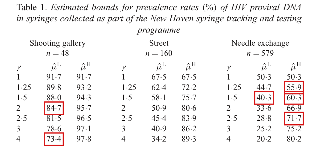
  • Table 1. All 42 entries are reproduced from the proportions 0.9170.917, 0.6750.675 and 0.5030.503, and 36 of them from the counts (see P025-N003). The rows γ=1\gamma=1 equal the reported percentages.
  • Section 4, on the rows of Table 1. The shooting gallery and needle exchange intervals are disjoint at γ=3\gamma=3 and overlap at γ=4\gamma=4, and the street and needle exchange intervals are disjoint at γ=1.25\gamma=1.25 and overlap at γ=1.5\gamma=1.5. The direction of selection described in the last sentence is the right one.
  • Section 5 presents its three extensions as proposals, and no contradiction with the results was found.
  • The numbered equations, assumptions, lemma, propositions and table are cited consistently in the article and in the supplementary material, and the supplementary material contains the proofs that the article says it contains.

My check did not cover the following. The article of Kaplan (1991) could not be obtained. The numbers of needles tested and of positive tests in Section 4 agree with indexed passages of a later report by the same investigator, and the numbers of needles returned were not compared with any source. Brewer (1979), Hajek (1971) and the other cited works were not read, and four reference entries were compared with public bibliographic records only (see P025-E007). The page of the comment of Hajek was not located. Whether the selection of the needle samples satisfies a bound γ\gamma cannot be checked from the article. I could not check replication code or original data; neither was available to me. The article reports no simulations.

Headline claims and related corrections

  1. When every selection probability lies in [α,β][\alpha,\beta], the attainable values of the Hajek estimate form exactly [μ^L,μ^H][\hat\mu^{\mathrm L},\hat\mu^{\mathrm H}]. The endpoints are attained by threshold weight vectors whose cut points kLk^{\mathrm L} and kHk^{\mathrm H} are given by explicit rules.

    Summary; Section 3.1; Proposition 1; equations (2)-(5); Appendix

    See P025-E001, P025-E004, P025-N001.

  2. The bounds depend on α\alpha and β\beta only through γ=β/α\gamma=\beta/\alpha. At γ=1\gamma=1 they equal the equal-probability estimate, so varying γ\gamma gives a nonparametric sensitivity analysis for departures from equal-probability sampling.

    Section 1; Section 3.1, equation (5) and the paragraph after it; Table 1

  3. The threshold weight vectors assign equal weights to tied outcomes. For a binary outcome with sample proportion pp, the interval is [p/(γ(1−p)+p), γp/((1−p)+γp)][p/(\gamma(1-p)+p),\,\gamma p/((1-p)+\gamma p)].

    Section 3.1, Lemma 1 and the unnumbered display after it; supplement p. 1; underlies Table 1

  4. Under Brewer’s replicated-population scaling, the population mean is identified up to [μ−,μ+][\mu_-,\mu_+], obtained by the same optimization using class totals Πj\Pi_j. These bounds are sharp in the limit and have the same threshold form.

    Section 1 ('yields sharp bounds on the population mean'); Section 3.2; Assumption 1; Proposition 2; equations (6)-(7); supplement pp. 1-2

    See P025-E001, P025-E002, P025-N002.

  5. Under Assumptions 1 and 2, the estimated bounds converge almost surely to μ+\mu_+ and μ−\mu_-, giving an asymptotically sharp interval estimator for the population mean.

    Section 3.2; Proposition 3; Assumptions 1 and 2; supplement p. 2, equations (B3)-(B4)

    See P025-E004, P025-E005, P025-N007.

  6. Table 1 gives bounds on HIV prevalence in the shooting gallery, street and needle exchange samples for γ\gamma between 11 and 44.

    Section 4; Table 1; dichotomous closed form

    See P025-N003.

  7. The needle data indicate that the gallery and exchange prevalence intervals overlap only when γ>3\gamma>3, and the street and exchange intervals when γ>1.25\gamma>1.25. The paper infers that equal prevalence in gallery and exchange needles would require infected gallery needles to be more than three times as likely to be tested as uninfected ones, with the reverse selection pattern for exchange needles.

    Summary; Section 4, pp. 238-239; Table 1

    See P025-E003, P025-A001, P025-N006.

Corrections

Moderate (2)

A real substantive error with limited reach.

In the rules that define the lower cut points kLk^{\mathrm L} and k−k_-, the inequality ⩾\geqslant should read ⩽\leqslant.

Proposition 1, the rule that defines kLk^{\mathrm L}, p. 236 (PDF p. 2); Proposition 2, the rule that defines k−k_-, p. 238 (PDF p. 4)

See also under Formal statements (Lean): P025-T1, P025-T2, P025-T3, P025-T4, P025-T7, P025-T9, P025-T19

As printed

Proposition 1, p. 236. An optimal solution to (3) is wL=(1/α,…,1/α,1/β,…,1/β)w^{\mathrm L} = (1/\alpha, \ldots, 1/\alpha, 1/\beta, \ldots, 1/\beta), where the first kLk^{\mathrm L} entries equal 1/α1/\alpha and the remaining n−kLn - k^{\mathrm L} entries equal 1/β1/\beta, with kLk^{\mathrm L} being the smallest nonnegative integer kk that satisfies {γ∑i=1kyi+∑i=k+1nyi}/{γk+(n−k)}⩾yk+1\{\gamma \sum_{i=1}^{k} y_i + \sum_{i=k+1}^{n} y_i\}/\{\gamma k + (n - k)\} \colorbox{#ffe58a}{$\geqslant$} y_{k+1}. The lower bound on μ^\hat\mu is therefore

μ^L=γ∑i=1kLyi+∑i=kL+1nyiγkL+(n−kL).\hat\mu^{\mathrm L} = \frac{\gamma \sum_{i=1}^{k^{\mathrm L}} y_i + \sum_{i=k^{\mathrm L}+1}^{n} y_i}{\gamma k^{\mathrm L} + (n - k^{\mathrm L})}.

Proposition 2, p. 238. and k−k_- is the smallest nonnegative integer kk satisfying

γ∑j=1kΠjy(j)+∑j=k+1∣Y∣Πjy(j)γ∑j=1kΠj+∑j=k+1∣Y∣Πj⩾y(k+1).\frac{\gamma \sum_{j=1}^{k} \Pi_j y_{(j)} + \sum_{j=k+1}^{|Y|} \Pi_j y_{(j)}}{\gamma \sum_{j=1}^{k} \Pi_j + \sum_{j=k+1}^{|Y|} \Pi_j} \colorbox{#ffe58a}{$\displaystyle \geqslant$} y_{(k+1)}.
The problem

The outcomes are in increasing order. At k=0k=0 the left side of the printed inequality is the sample mean in Proposition 1, and the Π\Pi-weighted mean of the distinct outcomes in Proposition 2. Since neither is smaller than the smallest outcome, k=0k=0 satisfies the printed inequality in every case, and both printed rules return the cut point 00. The vector wLw^{\mathrm L}, or W−W_-, then has every entry equal to 1/β1/\beta. Evaluating these vectors in (3) and (7) gives the unweighted sample mean and the Π\Pi-weighted mean, respectively. When γ>1\gamma>1 and the outcomes are not all equal, this vector does not minimize (3) or (7), since a larger weight on the smallest outcome lowers the ratio. The left endpoint of (5), computed with the printed kLk^{\mathrm L}, then leaves out values that μ^\hat\mu can take. The paper does not display the correct rule elsewhere. The Appendix says that the solution to (3) “can be derived in a similar manner”, and the supplementary proof of Proposition 2 treats μ+\mu_+ only. When γ=1\gamma=1 or all outcomes are equal, the ratio has the same value at every feasible weight vector, and the printed rules return a minimizer.

Evidence an exact counterexample

The evidence is an exact counterexample for each proposition and a derivation of the corrected rule.

Counterexample. Let y=(0,1)y=(0,1), α=1/2\alpha=1/2 and β=1\beta=1, so that γ=2\gamma=2. I write (u,v)=(βw1,βw2)∈[1,2]2(u,v)=(\beta w_1,\beta w_2)\in[1,2]^2 for the scaled weights. The ratio in (3) is v/(u+v)v/(u+v). The printed rule accepts k=0k=0, since 1/2⩾01/2\geqslant 0, and returns wL=(1,1)w^{\mathrm L}=(1,1) and μ^L=1/2\hat\mu^{\mathrm L}=1/2. For all (u,v)∈[1,2]2(u,v)\in[1,2]^2, I have

vu+v−13=(2−u)+2(v−1)3(u+v)⩾0,\frac{v}{u+v}-\frac13=\frac{(2-u)+2(v-1)}{3(u+v)}\geqslant 0,

with equality at (u,v)=(2,1)(u,v)=(2,1). The minimum of (3) is 1/31/3, and the printed lower bound exceeds it by 1/61/6. For Proposition 2, I consider a population of two units with outcomes (0,1)(0,1) and selection probabilities (1/2,1)(1/2,1). Then (Π1,Π2)=(1/2,1)(\Pi_1,\Pi_2)=(1/2,1), the ratio in (7) is v/(u/2+v)v/(u/2+v), and

vu/2+v−12=(2−u)+2(v−1)2(u+2v)⩾0.\frac{v}{u/2+v}-\frac12=\frac{(2-u)+2(v-1)}{2(u+2v)}\geqslant 0 .

The minimum of (7) is 1/21/2, which is the population mean, and the ratio at the printed W−=(1,1)W_-=(1,1) is 2/32/3. The table lists the values at the four vertices.

Value of the ratio at the vertices of the box of scaled weights [1,2]2[1,2]^2, for outcomes (0,1)(0,1), α=1/2\alpha=1/2 and β=1\beta=1.
Scaled weights (u,v)(u,v)Proposition 1, ratio in (3)Proposition 2 with Π=(1/2,1)\Pi=(1/2,1), ratio in (7)
(1,1)(1,1), printed rule, k=0k=01/21/22/32/3
(1,2)(1,2)2/32/34/54/5
(2,1)(2,1), corrected rule, k=1k=11/31/31/21/2
(2,2)(2,2)1/21/22/32/3

Derivation of the corrected rule. Both propositions are instances of one problem. Let x1⩽⋯⩽xmx_1\leqslant\cdots\leqslant x_m, let aj>0a_j>0, and let γ⩾1\gamma\geqslant 1. Proposition 1 has m=nm=n, xj=yjx_j=y_j and aj=1a_j=1, and Proposition 2 has m=∣Y∣m=|Y|, xj=y(j)x_j=y_{(j)} and aj=Πja_j=\Pi_j. After the weights are multiplied by β\beta, the lower problem is to minimize

R(q)=∑j=1majqjxj∑j=1majqjover 1⩽qj⩽γ.R(q)=\frac{\sum_{j=1}^{m}a_jq_jx_j}{\sum_{j=1}^{m}a_jq_j}\qquad\text{over } 1\leqslant q_j\leqslant\gamma .

For 0⩽k⩽m0\leqslant k\leqslant m, I define

Dk=γ∑j=1kaj+∑j=k+1maj,Bk=γ∑j=1kajxj+∑j=k+1majxj,Fk=BkDk,D_k=\gamma\sum_{j=1}^{k}a_j+\sum_{j=k+1}^{m}a_j,\qquad B_k=\gamma\sum_{j=1}^{k}a_jx_j+\sum_{j=k+1}^{m}a_jx_j,\qquad F_k=\frac{B_k}{D_k},

so that FkF_k is the left side of the inequality in each rule. By these definitions, I have

Fk+1−Fk=(γ−1) ak+1 (xk+1−Fk)Dk+1for 0⩽k<m.F_{k+1}-F_k=\frac{(\gamma-1)\,a_{k+1}\,(x_{k+1}-F_k)}{D_{k+1}}\qquad\text{for } 0\leqslant k<m .

For γ>1\gamma>1, the value FkF_k decreases at the step kk exactly when Fk>xk+1F_k>x_{k+1}. Let k∗k_* be the smallest k∈{0,…,m−1}k\in\{0,\ldots,m-1\} such that Fk⩽xk+1F_k\leqslant x_{k+1}. Such a kk exists, since Fm−1F_{m-1} is a weighted average of outcomes that are at most xmx_m. I set λ=Fk∗\lambda=F_{k_*}, and qj∗=γq^*_j=\gamma for j⩽k∗j\leqslant k_* and qj∗=1q^*_j=1 for j>k∗j>k_*. If k∗>0k_*>0, then Fk∗−1>xk∗F_{k_*-1}>x_{k_*} because k∗k_* is the smallest such index, and

Fk∗−xk∗=Dk∗−1 (Fk∗−1−xk∗)Dk∗>0.F_{k_*}-x_{k_*}=\frac{D_{k_*-1}\,(F_{k_*-1}-x_{k_*})}{D_{k_*}}>0 .

It follows that xj<λx_j<\lambda for all j⩽k∗j\leqslant k_*, and xj⩾xk∗+1⩾λx_j\geqslant x_{k_*+1}\geqslant\lambda for all j>k∗j>k_*. Let qq be any feasible vector. For j⩽k∗j\leqslant k_*, I have qj−qj∗⩽0q_j-q^*_j\leqslant 0 and xj−λ<0x_j-\lambda<0, and for j>k∗j>k_*, I have qj−qj∗⩾0q_j-q^*_j\geqslant 0 and xj−λ⩾0x_j-\lambda\geqslant 0. Since ∑jajqj∗(xj−λ)=0\sum_ja_jq^*_j(x_j-\lambda)=0, I obtain

R(q)−λ=∑jaj(qj−qj∗)(xj−λ)∑jajqj⩾0.R(q)-\lambda=\frac{\sum_{j}a_j(q_j-q^*_j)(x_j-\lambda)}{\sum_{j}a_jq_j}\geqslant 0 .

The vector q∗q^* minimizes RR over the whole box, including when outcomes are tied and when γ=1\gamma=1.

What survives

The correction needs no new assumption. The definitions (2), (3), (6) and (7), the rules for kHk^{\mathrm H} and k+k_+, the upper bounds, and the closed form for dichotomous outcomes are unaffected by this sign correction. All 42 entries of Table 1 are reproduced from the reported percentages by the closed form, and this sign correction does not change the table. The estimated bounds still converge to the limits defined by (6) and (7). The rules for kLk^{\mathrm L} and k−k_- change, and with them the left endpoint of (5) and computations of the lower bound that use either printed rule. The summation limits in the displayed formula for μ−\mu_- are corrected separately in P025-E002.

Corrected

Proposition 1, p. 236. Let γ=β/α⩾1\gamma=\beta/\alpha\geqslant 1 and y1⩽⋯⩽yny_1\leqslant\cdots\leqslant y_n. An optimal solution to (3) is wL=(1/α,…,1/α,1/β,…,1/β)w^{\mathrm L} = (1/\alpha, \ldots, 1/\alpha, 1/\beta, \ldots, 1/\beta), where the first kLk^{\mathrm L} entries equal 1/α1/\alpha and the remaining n−kLn - k^{\mathrm L} entries equal 1/β1/\beta, with kLk^{\mathrm L} being the smallest integer kk with 0⩽k<n0\leqslant k<n that satisfies {γ∑i=1kyi+∑i=k+1nyi}/{γk+(n−k)}⩽yk+1\{\gamma \sum_{i=1}^{k} y_i + \sum_{i=k+1}^{n} y_i\}/\{\gamma k + (n - k)\} \colorbox{#ffe58a}{$\leqslant$} y_{k+1}. The lower bound on μ^\hat\mu is therefore

μ^L=γ∑i=1kLyi+∑i=kL+1nyiγkL+(n−kL).\hat\mu^{\mathrm L} = \frac{\gamma \sum_{i=1}^{k^{\mathrm L}} y_i + \sum_{i=k^{\mathrm L}+1}^{n} y_i}{\gamma k^{\mathrm L} + (n - k^{\mathrm L})}.

Proposition 2, p. 238. Let y(1)<⋯<y(∣Y∣)y_{(1)}<\cdots<y_{(|Y|)} and Πj>0\Pi_j>0 be as in Section 3.2. Then k−k_- is the smallest integer kk with 0⩽k<∣Y∣0\leqslant k<|Y| satisfying

γ∑j=1kΠjy(j)+∑j=k+1∣Y∣Πjy(j)γ∑j=1kΠj+∑j=k+1∣Y∣Πj⩽y(k+1).\frac{\gamma \sum_{j=1}^{k} \Pi_j y_{(j)} + \sum_{j=k+1}^{|Y|} \Pi_j y_{(j)}}{\gamma \sum_{j=1}^{k} \Pi_j + \sum_{j=k+1}^{|Y|} \Pi_j} \colorbox{#ffe58a}{$\displaystyle \leqslant$} y_{(k+1)}.

In each rule the last index, k=n−1k=n-1 or k=∣Y∣−1k=|Y|-1, satisfies the inequality, and the cut point exists.

Crop of the second half of Proposition 1, from An optimal solution to (3) to the displayed formula for the lower bound. A red outline surrounds the greater-than-or-equal sign that stands before y sub k plus 1 in the third line.
Proposition 1, p. 236 (PDF p. 2). The outline marks the inequality sign in the rule that defines kLk^{\mathrm L}.
Crop of the line and k minus is the smallest nonnegative integer k satisfying, followed by a displayed ratio of sums. A red outline surrounds the greater-than-or-equal sign between the ratio and y sub (k plus 1).
Proposition 2, p. 238 (PDF p. 4), directly below Table 1. The outline marks the inequality sign in the rule that defines k−k_-.

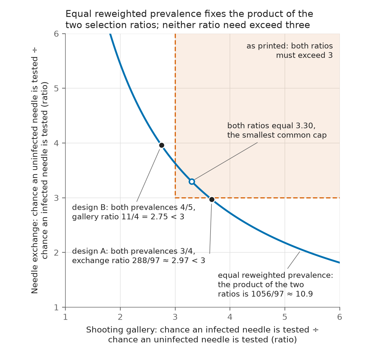
For the shooting gallery and needle exchange intervals to overlap, the common bound γ\gamma must be at least about 3.303.30; neither individual selection ratio needs to exceed three.

Section 4, last sentence, pp. 238–239 (PDF pp. 4–5)

See also under Formal statements (Lean): P025-T5, P025-T6

As printed

This means that for the shooting gallery needles to possibly show the same HIV prevalence rate as the exchange needles, infected shooting gallery needles must have been more than three times as likely to be tested than uninfected shooting gallery needles, with the converse holding for exchange needles.

The problem

The sentence makes two claims about the selection of the samples. It says that infected shooting gallery needles were more than three times as likely to be tested as uninfected ones, and that uninfected exchange needles were more than three times as likely to be tested as infected ones. Table 1 does not show this. The parameter γ\gamma is a common bound on how far the selection probabilities may differ within a population. On p. 236 the paper says that γ=5\gamma=5 “indicates that some units may be up to five times more likely to be sampled than others”. The table shows that the two intervals overlap only when this bound is larger than three. It says nothing about the ratio that each sample attains. Equal reweighted estimates fix the product of the two effective ratios, which must equal the odds ratio of the two sample proportions, about 10.910.9. The product can be split unevenly, and one ratio can be below three when the other is larger. The paper does not assume that the two ratios are equal.

Evidence an exact counterexample

The evidence is a derivation and two exact designs.

Derivation. Let a sample have an infected fraction pp, and write π1\pi_1 and π0\pi_0 for the effective probabilities obtained by averaging inverse selection probabilities within each sampled infection group and taking reciprocals. By (1), the Hajek estimate qq of the prevalence satisfies q/(1−q)={p/(1−p)}(π0/π1)q/(1-q)=\{p/(1-p)\}(\pi_0/\pi_1). I write rG=πG,1/πG,0r_G=\pi_{G,1}/\pi_{G,0} for the shooting gallery and rE=πE,0/πE,1r_E=\pi_{E,0}/\pi_{E,1} for the needle exchange. The two estimates are equal exactly when

rG rE=pG(1−pE)(1−pG) pE.r_G\,r_E=\frac{p_G(1-p_E)}{(1-p_G)\,p_E}.

With the printed proportions 0.9170.917 and 0.5030.503, the right side is 455749/41749≈10.92455749/41749\approx 10.92, and with the count-derived proportions 44/4844/48 and 291/579291/579, it is 1056/97≈10.891056/97\approx 10.89. By the closed form on p. 237, the two intervals overlap exactly when γ2\gamma^2 is at least this number. The condition is γ⩾455749/41749≈3.304\gamma\geqslant\sqrt{455749/41749}\approx 3.304 with the printed proportions and γ⩾1056/97≈3.299\gamma\geqslant\sqrt{1056/97}\approx 3.299 with the count-derived proportions. At the smallest such γ\gamma both ratios equal γ\gamma, and at a larger bound, such as the row γ=4\gamma=4 of Table 1, they can differ.

Two designs. In each design below, a fixed number of needles is drawn uniformly from the infected and from the uninfected needles of each population. The samples have the sizes 4848 and 579579 reported in Section 4 and positive counts 4444 and 291291 implied by rounding its percentages to the nearest tenth of a percent. The two populations have the same prevalence, the two Hajek estimates equal this prevalence on every draw, and all selection probabilities lie in [1/4,1][1/4,1], so that γ=4\gamma=4. In design A the ratio for the needle exchange is below three, and in design B the ratio for the shooting gallery is below three. The conclusion is the same for two further choices of the selection probabilities, with the proportions 0.9170.917 and 0.5030.503 taken as exact. There the ratios (rG,rE)(r_G,r_E) are (917/249, 1491/503)(917/249,\ 1491/503) at prevalence 3/43/4, with 1491/503<31491/503<3, and (917/332, 1988/503)(917/332,\ 1988/503) at prevalence 4/54/5, with 917/332<3917/332<3.

Two exact designs with equal prevalence in which one selection ratio is below three. Pairs are (infected, uninfected). The ratio is rGr_G for the shooting gallery and rEr_E for the needle exchange.
DesignPopulationTestedSelection probabilitiesRatioPrevalence
A, gallery(48,16)(48,16)(44,4)(44,4)(11/12, 1/4)(11/12,\ 1/4)11/3≈3.6711/3\approx 3.673/43/4
A, exchange(864,288)(864,288)(291,288)(291,288)(97/288, 1)(97/288,\ 1)288/97≈2.97288/97\approx 2.973/43/4
B, gallery(48,12)(48,12)(44,4)(44,4)(11/12, 1/3)(11/12,\ 1/3)11/4=2.7511/4=2.754/54/5
B, exchange(1156,289)(1156,289)(291,288)(291,288)(291/1156, 288/289)(291/1156,\ 288/289)384/97≈3.96384/97\approx 3.964/54/5
What survives

Table 1 is unchanged, and so is the statement that the shooting gallery and needle exchange intervals overlap only when γ>3\gamma>3, with the first overlap in the table at γ=4\gamma=4. The comparison of the street and needle exchange samples and the method of sensitivity analysis are unaffected. I replace the inference in the last sentence about the two selection processes by a weaker statement about the common bound, without adding an assumption.

Corrected

For the shooting gallery and needle exchange interval estimates to overlap, the common bound on the ratios of selection probabilities must be at least about 3⋅303{\cdot}30. This does not require both populations' actual directional selection ratios to exceed three. With the printed proportions 0⋅9170{\cdot}917 and 0⋅5030{\cdot}503, equal reweighted estimates require that the product of the two effective ratios, for infected against uninfected shooting gallery needles and for uninfected against infected exchange needles, equal 455749/41749455749/41749, which is about 10⋅910{\cdot}9.

Crop of the last three lines of page 238, which contain the sentence on when the intervals overlap. A red outline surrounds the words This means that for the shooting gallery needles to possibly show the same, which begin the last sentence of Section 4 and run to the end of the page.
Section 4, start of the last sentence, foot of p. 238 (PDF p. 4). The outline marks the words “This means that for the shooting gallery needles to possibly show the same”, which follow the two statements about overlap.
Crop of the first three lines of page 239, which complete the last sentence of Section 4. Red outlines surround the words must have been more than at the end of the first line and three times as likely at the start of the second, and the words with the converse holding for at the end of the second line and exchange needles at the start of the third.
Section 4, end of the last sentence, p. 239 (PDF p. 5). The outlines mark the words “must have been more than three times as likely” and “with the converse holding for exchange needles”.
A plot with the shooting gallery ratio, infected against uninfected, on the horizontal axis and the needle exchange ratio, uninfected against infected, on the vertical axis, both from 1 to 6. A blue curve of constant product 1056/97, about 10.9, falls from the upper left to the lower right. A shaded square with a dashed orange border covers the region where both ratios exceed 3 and is labelled as printed: both ratios must exceed 3. The curve enters the shaded region through its left edge, passes through the open point near (3.30, 3.30), labelled the smallest common cap, and exits through the bottom edge. Two filled points on the curve lie outside the region: design B at gallery ratio 11/4 = 2.75 with both prevalences 4/5, and design A at exchange ratio 288/97, about 2.97, with both prevalences 3/4. The title reads Equal reweighted prevalence fixes the product of the two selection ratios; neither ratio need exceed three.
The pairs of selection ratios for which the shooting gallery and needle exchange samples have equal reweighted prevalence, computed from the count-derived proportions 44/4844/48 and 291/579291/579. The curve is the set of pairs whose product is 1056/971056/97. The shaded region is what the printed sentence asserts. The filled points are designs A and B of the table, and the open point is the pair at which both ratios equal 1056/97≈3.30\sqrt{1056/97}\approx 3.30.

Minor (6)

Real but inconsequential, for example a misprint that does not change a result.

In the displayed formula for μ−\mu_-, both tail sums should start at j=k−+1j=k_-+1, not at j=k−−1j=k_--1.

Proposition 2, displayed formula for μ−\mu_-, p. 237 (PDF p. 3)

See also under Formal statements (Lean): P025-T2, P025-T4, P025-T9, P025-T10

As printed
μ−=γ∑j=1k−Πjy(j)+∑j=k−−1∣Y∣Πjy(j)γ∑j=1k−Πj+∑j=k−−1∣Y∣Πj,\mu_- = \frac{\gamma \sum_{j=1}^{k_-} \Pi_j y_{(j)} + \sum_{j=\colorbox{#ffe58a}{$\displaystyle \scriptstyle k_- -1$}}^{|Y|} \Pi_j y_{(j)}}{\gamma \sum_{j=1}^{k_-} \Pi_j + \sum_{j=\colorbox{#ffe58a}{$\displaystyle \scriptstyle k_- -1$}}^{|Y|} \Pi_j},
The problem

Proposition 2 states that the first k−k_- entries of W−W_- equal 1/α1/\alpha and the remaining ∣Y∣−k−|Y|-k_- entries equal 1/β1/\beta. The value of (7) at W−W_- therefore has the classes j⩽k−j\leqslant k_- with the factor γ\gamma and the classes j⩾k−+1j\geqslant k_-+1 without it. As printed, the second sums start at k−−1k_--1. For k−⩾2k_-\geqslant 2, the classes k−−1k_--1 and k−k_- are counted in both sums, and for k−=0k_-=0 or k−=1k_-=1, the lower limit is an index with no class. The displays for μ+\mu_+, for the cut points and in Assumption 2 start their second sums at k+1k+1.

Evidence an exact counterexample

The evidence is a substitution and an exact example. For 0⩽k⩽∣Y∣0\leqslant k\leqslant|Y|, let W(k)W^{(k)} have its first kk entries equal to 1/α1/\alpha and the others equal to 1/β1/\beta. Substituting W(k)W^{(k)} into the ratio in (7) and multiplying the numerator and the denominator by β\beta, I obtain

γ∑j=1kΠjy(j)+∑j=k+1∣Y∣Πjy(j)γ∑j=1kΠj+∑j=k+1∣Y∣Πj,\frac{\gamma\sum_{j=1}^{k}\Pi_jy_{(j)}+\sum_{j=k+1}^{|Y|}\Pi_jy_{(j)}}{\gamma\sum_{j=1}^{k}\Pi_j+\sum_{j=k+1}^{|Y|}\Pi_j},

which is the corrected display at k=k−k=k_-. For the example, let α=1/2\alpha=1/2, β=1\beta=1, and let the population have outcomes (0,0,1,1,2,3)(0,0,1,1,2,3) and selection probabilities (1/2,1/2,1/2,1/2,1,1)(1/2,1/2,1/2,1/2,1,1). The distinct outcomes are (0,1,2,3)(0,1,2,3) and Π=(1,1,1,1)\Pi=(1,1,1,1). With the weights scaled by β\beta, the ratio in (7) is F(W)=(W2+2W3+3W4)/(W1+W2+W3+W4)F(W)=(W_2+2W_3+3W_4)/(W_1+W_2+W_3+W_4) on [1,2]4[1,2]^4, and

F(W)−76=7(2−W1)+(2−W2)+5(W3−1)+11(W4−1)6(W1+W2+W3+W4)⩾0,F(W)-\frac76=\frac{7(2-W_1)+(2-W_2)+5(W_3-1)+11(W_4-1)}{6(W_1+W_2+W_3+W_4)}\geqslant 0 ,

with equality only at W=(2,2,1,1)W=(2,2,1,1). The minimum of (7) is 7/67/6, and it is attained at the cut point k−=2k_-=2. At k−=2k_-=2 the printed display equals {2(0+1)+(0+1+2+3)}/{2(1+1)+(1+1+1+1)}=1\{2(0+1)+(0+1+2+3)\}/\{2(1+1)+(1+1+1+1)\}=1, and the corrected display equals {2(0+1)+(2+3)}/{2(1+1)+(1+1)}=7/6\{2(0+1)+(2+3)\}/\{2(1+1)+(1+1)\}=7/6.

What survives

The definitions (6) and (7), the description of W−W_-, the bounds of Section 3.1 and Table 1 are unaffected. The supplementary material works with the full weighted sums and does not use the printed limits. The rule that selects k−k_- is corrected in P025-E001.

Corrected

With k−k_- and W−W_- as in Proposition 2, the value of (7) at W−W_- is

μ−=γ∑j=1k−Πjy(j)+∑j=k−+1∣Y∣Πjy(j)γ∑j=1k−Πj+∑j=k−+1∣Y∣Πj,\mu_- = \frac{\gamma \sum_{j=1}^{k_-} \Pi_j y_{(j)} + \sum_{j=\colorbox{#ffe58a}{$\displaystyle \scriptstyle k_- +1$}}^{|Y|} \Pi_j y_{(j)}}{\gamma \sum_{j=1}^{k_-} \Pi_j + \sum_{j=\colorbox{#ffe58a}{$\displaystyle \scriptstyle k_- +1$}}^{|Y|} \Pi_j},

where a sum over an empty range is zero.

Crop of the first line of Proposition 2 and the two displayed formulas for mu plus and mu minus. Red outlines surround the two lower summation limits j equals k minus, minus 1, in the numerator and in the denominator of the formula for mu minus, on the right.
Proposition 2, p. 237 (PDF p. 3). The outlines mark the lower limits j=k−−1j=k_--1 of the second sums in the numerator and the denominator of the formula for μ−\mu_-.

The Appendix argument for kHk^{\mathrm H}, and the steps (B1) and (B2) of the supplementary material, hold for γ>1\gamma>1; the case γ=1\gamma=1 needs a separate sentence.

Appendix, proof of Proposition 1, pp. 239–240 (PDF pp. 5–6); supplementary material, proof of Proposition 2, (B1) and (B2), p. 2

See also under Formal statements (Lean): P025-T11, P025-T12

As printed

Appendix, p. 239. Let wk=(1/β,…,1/β,1/α,…,1/α)w^k = (1/\beta, \ldots, 1/\beta, 1/\alpha, \ldots, 1/\alpha) where the first kk entries are 1/β1/\beta and the last n−kn - k are 1/α1/\alpha. Then (wk+1′y)/(wk+1′1n)−(wk′y)/(wk′1n)⩽0(w^{k+1\prime} y)/(w^{k+1\prime} 1_n) - (w^{k\prime} y)/(w^{k\prime} 1_n) \leqslant 0 implies that

∑i=1kyi+γ∑i=k+1nyik+γ(n−k)⩽yk+1.\frac{\sum_{i=1}^{k} y_i + \gamma \sum_{i=k+1}^{n} y_i}{k + \gamma (n - k)} \leqslant y_{k+1}.

Appendix, p. 240. Thus

kH=min⁡{k⩾0:wk′ywk′1n⩾wk+1′ywk+1′1n}=min⁡{k⩾0:∑i=1kyi+γ∑i=k+1nyik+γ(n−k)⩽yk+1}.k^{\mathrm H} = \min\left\{ k \geqslant 0 : \frac{w^{k\prime} y}{w^{k\prime} 1_n} \geqslant \frac{w^{k+1\prime} y}{w^{k+1\prime} 1_n} \right\} \colorbox{#ffe58a}{$\displaystyle =$} \min\left\{ k \geqslant 0 : \frac{\sum_{i=1}^{k} y_i + \gamma \sum_{i=k+1}^{n} y_i}{k + \gamma (n - k)} \leqslant y_{k+1} \right\}.

Supplementary material, p. 2. Then the condition μ(1/β,1/β)>μ(1/α,1/β)\mu(1/\beta, 1/\beta) > \mu(1/\alpha, 1/\beta) is equivalent to

c2y(k)−c1+β−1Πk+1(y(k)−y(k+1))<0(B1)c_2 y_{(k)} - c_1 + \beta^{-1} \Pi_{k+1} (y_{(k)} - y_{(k+1)}) < 0 \qquad \text{(B1)}

and the condition μ(1/α,1/α)>μ(1/α,1/β)\mu(1/\alpha, 1/\alpha) > \mu(1/\alpha, 1/\beta) is equivalent to

c1−c2y(k+1)+α−1Πk(y(k)−y(k+1))<0.(B2)c_1 - c_2 y_{(k+1)} + \alpha^{-1} \Pi_k (y_{(k)} - y_{(k+1)}) < 0. \qquad \text{(B2)}
The problem

Proposition 1 allows γ=1\gamma=1, and Table 1 includes it. Let Fk=(wk′y)/(wk′1n)F_k=(w^{k\prime}y)/(w^{k\prime}1_n) and Dk=k+γ(n−k)D_k=k+\gamma(n-k). Then

Fk+1−Fk=(1−γ) (yk+1−Fk)Dk+1for 0⩽k<n.F_{k+1}-F_k=\frac{(1-\gamma)\,(y_{k+1}-F_k)}{D_{k+1}}\qquad\text{for } 0\leqslant k<n .

For γ>1\gamma>1, this identity implies that Fk+1−Fk⩽0F_{k+1}-F_k\leqslant 0 if and only if Fk⩽yk+1F_k\leqslant y_{k+1}, and the two minima on p. 240 agree. For γ=1\gamma=1, the vectors wkw^k coincide and the difference is zero for every kk. The printed implication and the equality of the two minima can then fail. The steps (B1) and (B2) have the same gap. Each difference of objective values equals 1/β−1/α1/\beta-1/\alpha times a positive factor times the left side of (B1) or (B2), and for α=β\alpha=\beta the difference is zero whatever the sign of that left side. The results are not affected. For γ=1\gamma=1 the only feasible weight vector has every entry equal to 1/α1/\alpha, both bounds in (2) and (3) equal the sample mean, and both (6) and (7) equal μ\mu.

Evidence an exact counterexample

The evidence is an exact counterexample to the four printed steps and the identities that show where γ>1\gamma>1 is used. Let n=N=2n=N=2, y=(0,1)y=(0,1) and α=β=1\alpha=\beta=1, so that γ=1\gamma=1 and w0=w1=w2=(1,1)w^0=w^1=w^2=(1,1). Then F0=F1=F2=1/2F_0=F_1=F_2=1/2. At k=0k=0, I have F1−F0=0⩽0F_1-F_0=0\leqslant 0, and the conclusion F0=1/2⩽y1=0F_0=1/2\leqslant y_1=0 is false. For k∈{0,1}k\in\{0,1\}, the first minimum on p. 240 is 00 and the second is 11. In the supplementary material, the two classes have y(1)=0y_{(1)}=0, y(2)=1y_{(2)}=1 and Π1=Π2=1\Pi_1=\Pi_2=1. With k=1k=1, I have c1=c2=0c_1=c_2=0, the left sides of (B1) and (B2) both equal −1-1, and μ(1/β,1/β)=μ(1/α,1/β)=μ(1/α,1/α)=1/2\mu(1/\beta,1/\beta)=\mu(1/\alpha,1/\beta)=\mu(1/\alpha,1/\alpha)=1/2. For the general case, let a=1/βa=1/\beta, b=1/αb=1/\alpha, p=Πkp=\Pi_k, q=Πk+1q=\Pi_{k+1}, and let E1E_1 and E2E_2 be the left sides of (B1) and (B2). A direct computation gives

μ(a,a)−μ(b,a)=(a−b) p E1(c2+ap+aq)(c2+bp+aq),μ(b,b)−μ(b,a)=(a−b) q E2(c2+bp+bq)(c2+bp+aq).\mu(a,a)-\mu(b,a)=\frac{(a-b)\,p\,E_1}{(c_2+ap+aq)(c_2+bp+aq)},\qquad \mu(b,b)-\mu(b,a)=\frac{(a-b)\,q\,E_2}{(c_2+bp+bq)(c_2+bp+aq)} .

Both denominators are positive. Since a−b<0a-b<0 for α<β\alpha<\beta, the two equivalences hold in this case. For α=β\alpha=\beta, both differences vanish.

What survives

The upper bound (4) and its optimal weights hold for all γ⩾1\gamma\geqslant 1. Lemma 1, Propositions 2 and 3, the closed form for dichotomous outcomes and Table 1 are unaffected by this boundary case; the rows γ=1\gamma=1 are the sample percentages. The identity for the sum of the left sides of (B1) and (B2) in the supplementary material is correct. One case is added to each proof, and no assumption or result changes.

Corrected

Appendix, proof of Proposition 1. If γ=1\gamma=1, then α=β\alpha=\beta and the only feasible weight vector is (1/α,…,1/α)(1/\alpha,\ldots,1/\alpha). The bounds in (2) and (3) then both equal the sample mean, the cut point kHk^{\mathrm H} of Proposition 1 selects this vector, and (4) holds. For the rest of the proof, assume that γ>1\gamma>1. Let wk=(1/β,…,1/β,1/α,…,1/α)w^k = (1/\beta, \ldots, 1/\beta, 1/\alpha, \ldots, 1/\alpha) where the first kk entries are 1/β1/\beta and the last n−kn - k are 1/α1/\alpha. Then, for 0⩽k<n0\leqslant k<n, (wk+1′y)/(wk+1′1n)−(wk′y)/(wk′1n)⩽0(w^{k+1\prime} y)/(w^{k+1\prime} 1_n) - (w^{k\prime} y)/(w^{k\prime} 1_n) \leqslant 0 if and only if

∑i=1kyi+γ∑i=k+1nyik+γ(n−k)⩽yk+1.\frac{\sum_{i=1}^{k} y_i + \gamma \sum_{i=k+1}^{n} y_i}{k + \gamma (n - k)} \leqslant y_{k+1}.

The display on p. 240 then holds as printed, with kk ranging over 0⩽k<n0\leqslant k<n.

Supplementary material, proof of Proposition 2. If α=β\alpha=\beta, then every feasible WjW_j equals 1/α1/\alpha, and (6) and (7) both equal μ\mu. For the rest of the proof, assume that α<β\alpha<\beta. Then the condition μ(1/β,1/β)>μ(1/α,1/β)\mu(1/\beta, 1/\beta) > \mu(1/\alpha, 1/\beta) is equivalent to (B1), and the condition μ(1/α,1/α)>μ(1/α,1/β)\mu(1/\alpha, 1/\alpha) > \mu(1/\alpha, 1/\beta) is equivalent to (B2).

Crop of the top of page 240: the word Thus, a displayed formula in which k superscript H equals a minimum over k of one condition, which equals a minimum over k of a second condition, and the sentence The solution to (3) can be derived in a similar manner. A red outline surrounds the equality sign between the two minima.
Appendix, end of the proof of Proposition 1, p. 240 (PDF p. 6). The outline marks the equality between the two minima that define kHk^{\mathrm H}.
Crop of three lines of the Appendix proof, ending Then the difference of two ratios is less than or equal to 0 implies that, followed by a displayed inequality with y sub k plus 1 on the right. Red outlines surround the less-than-or-equal sign at the end of the second line and the words 0 implies that at the start of the third.
Appendix, proof of Proposition 1, p. 239 (PDF p. 5). The outlines mark the words “⩽0\leqslant 0 implies that”, which precede the displayed inequality.
Crop of four lines of the supplementary material: Then the condition mu(1/beta, 1/beta) greater than mu(1/alpha, 1/beta) is equivalent to, the displayed inequality (B1), and the condition mu(1/alpha, 1/alpha) greater than mu(1/alpha, 1/beta) is equivalent to, and the displayed inequality (B2). Red outlines surround the words is equivalent to in the first and third lines.
Supplementary material, proof of Proposition 2, p. 2. The outlines mark the two occurrences of “is equivalent to” that introduce (B1) and (B2).

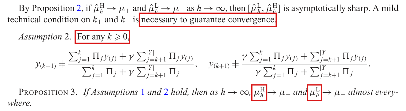
Assumption 2 is sufficient for the proof of Proposition 3 and is not necessary for the estimated bounds to converge; Proposition 3 should carry hats on the estimators, and Assumption 2 is meant for 0⩽k<∣Y∣0\leqslant k<|Y|.

Section 3.2, the sentence before Assumption 2, Assumption 2, and Proposition 3, p. 238 (PDF p. 4)

See also under Formal statements (Lean): P025-T13, P025-T14, P025-T21

As printed

A mild technical condition on k+k_+ and k−k_- is necessary to guarantee convergence.

Assumption 2. For any k⩾0k \geqslant 0,

y(k+1)≠∑j=1kΠjy(j)+γ∑j=k+1∣Y∣Πjy(j)∑j=1kΠj+γ∑j=k+1∣Y∣Πj,y(k+1)≠γ∑j=1kΠjy(j)+∑j=k+1∣Y∣Πjy(j)γ∑j=1kΠj+∑j=k+1∣Y∣Πj.y_{(k+1)} \neq \frac{\sum_{j=1}^{k} \Pi_j y_{(j)} + \gamma \sum_{j=k+1}^{|Y|} \Pi_j y_{(j)}}{\sum_{j=1}^{k} \Pi_j + \gamma \sum_{j=k+1}^{|Y|} \Pi_j}, \qquad y_{(k+1)} \neq \frac{\gamma \sum_{j=1}^{k} \Pi_j y_{(j)} + \sum_{j=k+1}^{|Y|} \Pi_j y_{(j)}}{\gamma \sum_{j=1}^{k} \Pi_j + \sum_{j=k+1}^{|Y|} \Pi_j}.

PROPOSITION 3. If Assumptions 1 and 2 hold, then as h→∞h \to \infty, μhH→μ+\colorbox{#ffe58a}{$\mu_h^{\mathrm H}$} \to \mu_+ and μhL→μ−\colorbox{#ffe58a}{$\mu_h^{\mathrm L}$} \to \mu_- almost everywhere.

The problem

There are three points. First, the estimated bounds μ^hH\hat\mu_h^{\mathrm H} and μ^hL\hat\mu_h^{\mathrm L} converge almost surely to μ+\mu_+ and μ−\mu_- under Assumption 1 alone. The supplementary material uses Assumption 2 to make the estimated cut point equal to k+k_+ for all large hh, which the convergence of the bounds does not require. Proposition 3 is correct as a statement of sufficient conditions, with a hypothesis that it does not need. Second, Proposition 3 prints μhH\mu_h^{\mathrm H} and μhL\mu_h^{\mathrm L} without hats. Assumption 1 defines the estimators μ^hH\hat\mu_h^{\mathrm H} and μ^hL\hat\mu_h^{\mathrm L}, and no quantity without a hat is defined. Third, y(k+1)y_{(k+1)} is defined only for 0⩽k<∣Y∣0\leqslant k<|Y|, and “for any k⩾0k\geqslant 0” includes indices at which Assumption 2 has no meaning.

Evidence an exact counterexample

The evidence is an exact example in which Assumption 2 fails and the bounds converge, a derivation that Assumption 1 suffices, and a check of the page for the hats and the range of kk.

Example. Let the population have outcomes (0,0,2,2,3,3)(0,0,2,2,3,3). Each replication selects one unit from each pair of units with equal outcomes, each with probability 1/21/2, and the three choices are independent. Then πi=1/2\pi_i=1/2 for all ii, and I take α=1/4\alpha=1/4 and β=1/2\beta=1/2, so that γ=2\gamma=2. The distinct outcomes are (0,2,3)(0,2,3) and Π=(1,1,1)\Pi=(1,1,1). After hh replications the sample contains exactly hh units at each outcome. With class weights (w0,w2,w3)∈[2,4]3(w_0,w_2,w_3)\in[2,4]^3, the ratio is f=(2w2+3w3)/(w0+w2+w3)f=(2w_2+3w_3)/(w_0+w_2+w_3) for the sample and in the limit, and

4(2w2+3w3)−5(w0+w2+w3)=3(w2−2)+7(w3−2)+5(4−w0)⩾0,2(w0+w2+w3)−(2w2+3w3)=2(w0−2)+(4−w3)⩾0.\begin{aligned} 4(2w_2+3w_3)-5(w_0+w_2+w_3)&=3(w_2-2)+7(w_3-2)+5(4-w_0)\geqslant 0,\\ 2(w_0+w_2+w_3)-(2w_2+3w_3)&=2(w_0-2)+(4-w_3)\geqslant 0 . \end{aligned}

By these two inequalities, I have 5/4⩽f⩽25/4\leqslant f\leqslant 2, with equality at (4,2,2)(4,2,2) and at (2,4,4)(2,4,4). I conclude that [μ^hL,μ^hH]=[μ−,μ+]=[5/4,2][\hat\mu_h^{\mathrm L},\hat\mu_h^{\mathrm H}]=[\mu_-,\mu_+]=[5/4,2] for every hh and every sample path. Assumption 2 fails at k=1k=1, since the first ratio there equals {1⋅0+2(2+3)}/{1+2(1+1)}=2=y(2)\{1\cdot 0+2(2+3)\}/\{1+2(1+1)\}=2=y_{(2)}.

Derivation. Let Ph,jP_{h,j} be the number of sampled units of outcome y(j)y_{(j)} after hh replications, divided by hh. By Assumption 1, the counts of class jj in the successive replications are independent and identically distributed, they are bounded, and their mean is Πj\Pi_j. The strong law of large numbers implies that Ph,j→ΠjP_{h,j}\to\Pi_j almost surely for every jj. For a vector pp with nonnegative entries and positive sum, I define

f(W,p)=∑jWjpjy(j)∑jWjpj,W∈B=[1/β,1/α]∣Y∣.f(W,p)=\frac{\sum_jW_jp_jy_{(j)}}{\sum_jW_jp_j},\qquad W\in B=[1/\beta,1/\alpha]^{|Y|}.

In (2) and (3) the weights of the units in one class can be replaced by their average, which lies in [1/β,1/α][1/\beta,1/\alpha]. Whenever the sample is nonempty, μ^hH=max⁡W∈Bf(W,Ph)\hat\mu_h^{\mathrm H}=\max_{W\in B}f(W,P_h) and μ^hL=min⁡W∈Bf(W,Ph)\hat\mu_h^{\mathrm L}=\min_{W\in B}f(W,P_h), and by (6) and (7), μ+=max⁡W∈Bf(W,Π)\mu_+=\max_{W\in B}f(W,\Pi) and μ−=min⁡W∈Bf(W,Π)\mu_-=\min_{W\in B}f(W,\Pi). Let R=y(∣Y∣)−y(1)R=y_{(|Y|)}-y_{(1)} and S=∑jΠjS=\sum_j\Pi_j. With m=f(W,p)m=f(W,p), I have

m−f(W,Π)=∑jWj(pj−Πj)(y(j)−m)∑jWjΠj,m-f(W,\Pi)=\frac{\sum_jW_j(p_j-\Pi_j)(y_{(j)}-m)}{\sum_jW_j\Pi_j},

and therefore

∣f(W,p)−f(W,Π)∣⩽γRS∑j∣pj−Πj∣for all W∈B.\bigl|f(W,p)-f(W,\Pi)\bigr|\leqslant\frac{\gamma R}{S}\sum_j|p_j-\Pi_j|\qquad\text{for all } W\in B .

In the last inequality, I used that ∣y(j)−m∣⩽R|y_{(j)}-m|\leqslant R and 1/β⩽Wj⩽1/α1/\beta\leqslant W_j\leqslant 1/\alpha. The maximum and the minimum over BB change by at most the same amount. With p=Php=P_h, I obtain μ^hH→μ+\hat\mu_h^{\mathrm H}\to\mu_+ and μ^hL→μ−\hat\mu_h^{\mathrm L}\to\mu_- almost surely, including when the ratios of Assumption 2 tie.

What survives

The conclusion of Proposition 3 holds, under Assumption 1 alone. The optimization problems (2), (3), (6) and (7), Table 1 and the application are unaffected. The sentence before Assumption 2 and the notation of Proposition 3 and Assumption 2 change.

Corrected

A mild technical condition on k+k_+ and k−k_- is sufficient for the proof of convergence.

Assumption 2. For every integer kk with 0⩽k<∣Y∣0 \leqslant k < |Y|,

y(k+1)≠∑j=1kΠjy(j)+γ∑j=k+1∣Y∣Πjy(j)∑j=1kΠj+γ∑j=k+1∣Y∣Πj,y(k+1)≠γ∑j=1kΠjy(j)+∑j=k+1∣Y∣Πjy(j)γ∑j=1kΠj+∑j=k+1∣Y∣Πj.y_{(k+1)} \neq \frac{\sum_{j=1}^{k} \Pi_j y_{(j)} + \gamma \sum_{j=k+1}^{|Y|} \Pi_j y_{(j)}}{\sum_{j=1}^{k} \Pi_j + \gamma \sum_{j=k+1}^{|Y|} \Pi_j}, \qquad y_{(k+1)} \neq \frac{\gamma \sum_{j=1}^{k} \Pi_j y_{(j)} + \sum_{j=k+1}^{|Y|} \Pi_j y_{(j)}}{\gamma \sum_{j=1}^{k} \Pi_j + \sum_{j=k+1}^{|Y|} \Pi_j}.

PROPOSITION 3. If Assumptions 1 and 2 hold, then as h→∞h \to \infty, μ^hH→μ+\colorbox{#ffe58a}{$\hat\mu_h^{\mathrm H}$} \to \mu_+ and μ^hL→μ−\colorbox{#ffe58a}{$\hat\mu_h^{\mathrm L}$} \to \mu_- almost everywhere.

The conclusion also holds without Assumption 2: if Assumption 1 holds, then as h→∞h\to\infty, μ^hH→μ+\hat\mu_h^{\mathrm H}\to\mu_+ and μ^hL→μ−\hat\mu_h^{\mathrm L}\to\mu_- almost everywhere.

Crop that begins By Proposition 2, shows Assumption 2 with its two displayed inequalities, and ends with Proposition 3. Red outlines surround four items: the words necessary to guarantee convergence in the second line, the words For any k greater than or equal to 0 at the start of Assumption 2, and in Proposition 3 the symbols mu sub h superscript H and mu sub h superscript L, neither of which has a hat.
Section 3.2, from the paragraph before Assumption 2 to Proposition 3, p. 238 (PDF p. 4). The outlines mark the words “necessary to guarantee convergence”, the words “For any k⩾0k\geqslant 0”, and the symbols μhH\mu_h^{\mathrm H} and μhL\mu_h^{\mathrm L}, which are printed without hats.

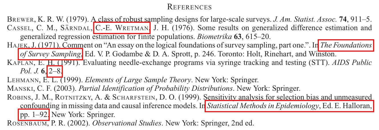
Four entries of the reference list need a correction: the separator before Wretman, the title of the volume that contains the comment of Hajek, the pages of Kaplan (1991), and the title, editors and pages of the volume that contains Robins et al.

References, entries for Cassel et al. (1976), Hajek (1971), Kaplan (1991) and Robins et al. (1999), p. 240 (PDF p. 6)

As printed

CASSEL, C. M., SÄRNDAL, C.-E. WRETMAN, J. H. (1976). Some results on generalized difference estimation and generalized regression estimation for finite populations. Biometrika 63, 615–20.

HAJEK, J. (1971). Comment on “An essay on the logical foundations of survey sampling, part one.”. In The Foundations of Survey Sampling, Ed. V. P. Godambe & D. A. Sprott, p. 246. Toronto: Holt, Rinehart, and Winston.

KAPLAN, E. H. (1991). Evaluating needle-exchange programs via syringe tracking and testing (STT). AIDS Public Pol. J. 6, 2–8.

ROBINS, J. M., ROTNITZKY, A. & SCHARFSTEIN, D. O. (1999). Sensitivity analysis for selection bias and unmeasured confounding in missing data and causal inference models. In Statistical Methods in Epidemiology, Ed. E. Halloran, pp. 1–92. New York: Springer.

The problem

The entry for Cassel et al. lacks the separator before the third author. The volume edited by Godambe and Sprott is Foundations of Statistical Inference. The article of Kaplan is on pp. 109–115 of its volume. The chapter of Robins et al. is on pp. 1–94 of Statistical Models in Epidemiology, the Environment, and Clinical Trials, edited by M. E. Halloran and D. Berry. Each cited work can still be identified, and no result or number depends on these entries.

Evidence a check of the printed page

I compared the printed entries with public bibliographic records. The publisher’s record for the volume of Halloran and Berry gives its title, its editors and the pages 11–9494 of the chapter (https://link.springer.com/book/10.1007/978-1-4612-1284-3). E. H. Kaplan’s list of his papers gives AIDS and Public Policy Journal 6:109–115, 1991 (https://faculty.som.yale.edu/edkaplan/papers/). Two library catalogues give the title Foundations of statistical inference: a symposium for the volume of 1971 edited by Godambe and Sprott (https://ci.nii.ac.jp/ncid/BA8882938X). No record that locates the comment of Hajek within that volume was found, and the page 246246 is left as printed. The publisher released the volume of Halloran and Berry in 1999 and dates its copyright 2000, and the year 1999 is not counted as an error.

What survives

The mathematics, the calculations and the citations in the text are unaffected.

Corrected

CASSEL, C. M., SÄRNDAL, C.-E. & WRETMAN, J. H. (1976). Some results on generalized difference estimation and generalized regression estimation for finite populations. Biometrika 63, 615–20.

HAJEK, J. (1971). Comment on “An essay on the logical foundations of survey sampling, part one.”. In Foundations of Statistical Inference, Ed. V. P. Godambe & D. A. Sprott, p. 246. Toronto: Holt, Rinehart, and Winston.

KAPLAN, E. H. (1991). Evaluating needle-exchange programs via syringe tracking and testing (STT). AIDS Public Pol. J. 6, 109–15.

ROBINS, J. M., ROTNITZKY, A. & SCHARFSTEIN, D. O. (1999). Sensitivity analysis for selection bias and unmeasured confounding in missing data and causal inference models. In Statistical Models in Epidemiology, the Environment, and Clinical Trials, Eds. M. E. Halloran & D. Berry, pp. 1–94. New York: Springer.

Crop of the reference list of the article, from Brewer (1979) to Rosenbaum (2002). Red outlines surround six items: the names C.-E. Wretman in the entry for Cassel, Sarndal and Wretman; the words The Foundations at the end of one line and of Survey Sampling at the start of the next in the entry for Hajek; the pages 2 to 8 in the entry for Kaplan; and the words Statistical Methods in Epidemiology, Ed. E. Halloran, and pp. 1 to 92 on the next line, in the entry for Robins, Rotnitzky and Scharfstein.
References, p. 240 (PDF p. 6). The outlines mark “C.-E. Wretman”, where the separator is missing, the volume title “The Foundations of Survey Sampling”, the pages “2–8”, and the clause “Statistical Methods in Epidemiology, Ed. E. Halloran, pp. 1–92”.

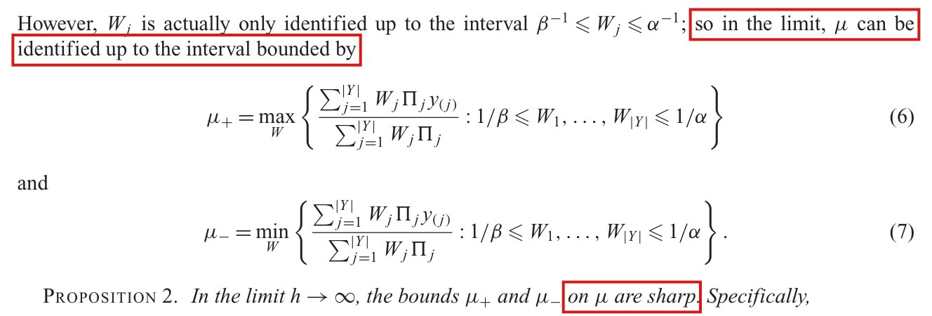
The bounds μ−\mu_- and μ+\mu_+ are sharp for the population mean relative to the limiting distribution of outcomes among sampled units, with the population size unrestricted, and the statement should name this information.

Section 3.2, first sentence, the sentence before (6), and the first sentence of Proposition 2, p. 237 (PDF p. 3)

See also under Formal statements (Lean): P025-T15, P025-T16

As printed

The proposed interval estimator yields asymptotically sharp bounds on μ\mu itself under the scaling proposed by Brewer (1979) and articulated in Assumption 1.

However, WjW_j is actually only identified up to the interval β−1⩽Wj⩽α−1\beta^{-1} \leqslant W_j \leqslant \alpha^{-1}; so in the limit, μ\mu can be identified up to the interval bounded by

μ+=max⁡W{∑j=1∣Y∣WjΠjy(j)∑j=1∣Y∣WjΠj:1/β⩽W1,…,W∣Y∣⩽1/α}(6)\mu_+ = \max_W \left\{ \frac{\sum_{j=1}^{|Y|} W_j \Pi_j y_{(j)}}{\sum_{j=1}^{|Y|} W_j \Pi_j} : 1/\beta \leqslant W_1, \ldots, W_{|Y|} \leqslant 1/\alpha \right\} \qquad (6)

and

μ−=min⁡W{∑j=1∣Y∣WjΠjy(j)∑j=1∣Y∣WjΠj:1/β⩽W1,…,W∣Y∣⩽1/α}.(7)\mu_- = \min_W \left\{ \frac{\sum_{j=1}^{|Y|} W_j \Pi_j y_{(j)}}{\sum_{j=1}^{|Y|} W_j \Pi_j} : 1/\beta \leqslant W_1, \ldots, W_{|Y|} \leqslant 1/\alpha \right\}. \qquad (7)

PROPOSITION 2. In the limit h→∞h \to \infty, the bounds μ+\mu_+ and μ−\mu_- on μ\mu are sharp. Specifically,

The problem

Proposition 2 and the first sentence of Section 3.2 call the interval [μ−,μ+][\mu_-,\mu_+] sharp for μ\mu and do not say relative to which information. The supplementary material shows that μ−\mu_- and μ+\mu_+ are the minimum and the maximum of the ratio over the box 1/β⩽Wj⩽1/α1/\beta\leqslant W_j\leqslant 1/\alpha. It does not show that populations compatible with what is observed in the limit have means that reach or approach these values, and whether they do depends on what is observed. The identification display on p. 237 names only the limiting shares qj=Πj/∑kΠkq_j=\Pi_j/\sum_k\Pi_k of the outcomes among sampled units. Relative to these shares, with the population size NN unrestricted, the claim holds when sharp means that μ−\mu_- and μ+\mu_+ are the infimum and the supremum of the compatible population means. The claim fails for richer information. The class sizes ∣Υj∣=WjΠj|\Upsilon_j|=W_j\Pi_j are positive integers. If the totals Πj\Pi_j themselves are retained, with fixed numerical α\alpha and β\beta, these integers lie in [Πj/β,Πj/α][\Pi_j/\beta,\Pi_j/\alpha], and if NN is known they sum to NN. The interval can then be strictly narrowed. The same qualification applies to the conclusion drawn from Proposition 2 on p. 238 and to the sentence of Section 1 discussed in P025-N001. In every case [μ−,μ+][\mu_-,\mu_+] contains μ\mu.

Evidence an exact counterexample

The evidence is two exact counterexamples to the unqualified claim and a derivation of the qualified one.

Totals retained, NN unknown. Let the population have outcomes (0,1,1)(0,1,1), and let each replication select one of the three samples of two units with probability 1/31/3. Every πi\pi_i equals 2/32/3, and I take α=1/2\alpha=1/2 and β=3/4\beta=3/4. The totals for the outcomes 00 and 11 are 2/32/3 and 4/34/3. The sizes m0m_0 and m1m_1 of the two classes satisfy 8/9⩽m0⩽4/38/9\leqslant m_0\leqslant 4/3 and 16/9⩽m1⩽8/316/9\leqslant m_1\leqslant 8/3, which implies that (m0,m1)=(1,2)(m_0,m_1)=(1,2) and μ=2/3\mu=2/3. Equations (6) and (7) give [μ−,μ+]=[4/7,3/4][\mu_-,\mu_+]=[4/7,3/4]. The gaps 2/3−4/7=2/212/3-4/7=2/21 and 3/4−2/3=1/123/4-2/3=1/12 do not depend on hh.

NN known. Let Π=(50,100)\Pi=(50,100) for the outcomes 00 and 11, α=1/10\alpha=1/10, β=1/5\beta=1/5 and N=1000N=1000. The class sizes satisfy 250⩽m0⩽500250\leqslant m_0\leqslant 500, 500⩽m1⩽1000500\leqslant m_1\leqslant 1000 and m0+m1=1000m_0+m_1=1000. The compatible means are m1/1000m_1/1000 with 500⩽m1⩽750500\leqslant m_1\leqslant 750, and each is attained by a design that selects 5050 zeros and 100100 ones uniformly. The sharp interval is [1/2,3/4][1/2,3/4], and the interval defined by (6) and (7) is [1/2,4/5][1/2,4/5].

Shares only, NN unrestricted. Let rj=∣Υj∣/Nr_j=|\Upsilon_j|/N be the population proportions, so that μ=∑jrjy(j)\mu=\sum_jr_jy_{(j)} and rj=Wjqj/∑kWkqkr_j=W_jq_j/\sum_kW_kq_k. As WW ranges over the box, rr ranges over the set

Cγ(q)={r: rj⩾0, ∑jrj=1, rjqk⩽γ rkqj for all j,k},\mathcal C_\gamma(q)=\Bigl\{r:\ r_j\geqslant 0,\ \sum_jr_j=1,\ r_jq_k\leqslant\gamma\,r_kq_j \text{ for all } j,k\Bigr\},

and μ−\mu_- and μ+\mu_+ are the minimum and the maximum of ∑jrjy(j)\sum_jr_jy_{(j)} over Cγ(q)\mathcal C_\gamma(q). Since every compatible population has r∈Cγ(q)r\in\mathcal C_\gamma(q), it satisfies μ−⩽μ⩽μ+\mu_-\leqslant\mu\leqslant\mu_+. Conversely, let r∈Cγ(q)r\in\mathcal C_\gamma(q) have rational coordinates, and let dd be an integer such that every drjdr_j is an integer. I consider a population with drjdr_j units of outcome y(j)y_{(j)}, each selected with probability tqj/rjtq_j/r_j, where tt satisfies

αmax⁡jrjqj⩽t⩽βmin⁡jrjqj.\alpha\max_j\frac{r_j}{q_j}\leqslant t\leqslant\beta\min_j\frac{r_j}{q_j}.

Such a tt exists because r∈Cγ(q)r\in\mathcal C_\gamma(q). These probabilities lie in [α,β][\alpha,\beta], the shares of the outcomes among sampled units are exactly qq, and the population mean is ∑jrjy(j)\sum_jr_jy_{(j)}. For γ>1\gamma>1, every inequality that defines Cγ(q)\mathcal C_\gamma(q) is strict at r=qr=q, which implies that the rational points are dense in Cγ(q)\mathcal C_\gamma(q). I conclude that the closure of the set of compatible population means is [μ−,μ+][\mu_-,\mu_+]. For γ=1\gamma=1, the set Cγ(q)\mathcal C_\gamma(q) is the point qq. In the first example, the shares are q=(1/3,2/3)q=(1/3,2/3), and both bounds are attained when only qq is retained. A population of three zeros, each selected with probability 1/21/2, and four ones, each selected with probability 3/43/4, has the mean 4/74/7. A population of one zero, selected with probability 3/43/4, and three ones, each selected with probability 1/21/2, has the mean 3/43/4.

What survives

The formulas (6) and (7), the form of the optimal weights, the bounds on the Hajek estimator, the convergence of the estimated bounds to μ−\mu_- and μ+\mu_+, Table 1 and the sensitivity analysis do not change. The interval [μ−,μ+][\mu_-,\mu_+] is a valid bound on μ\mu whatever else is known. The stronger claim does not hold. When NN or the totals per replication are also known, the interval can be narrowed. Sharpness also does not mean that every point of the interval is the mean of a finite population.

Corrected

The proposed interval estimator yields asymptotically sharp bounds on μ\mu itself under the scaling proposed by Brewer (1979) and articulated in Assumption 1, relative to the limiting distribution of the outcomes among sampled units.

However, WjW_j is actually only identified up to the interval β−1⩽Wj⩽α−1\beta^{-1} \leqslant W_j \leqslant \alpha^{-1}; so in the limit, given only the shares qj=Πj/∑k=1∣Y∣Πkq_j=\Pi_j/\sum_{k=1}^{|Y|}\Pi_k and with the population size NN unrestricted, μ\mu can be identified up to the interval bounded by μ+\mu_+ in (6) and μ−\mu_- in (7).

PROPOSITION 2. Let 0<α⩽β⩽10<\alpha\leqslant\beta\leqslant 1, and let qj=Πj/∑k=1∣Y∣Πkq_j=\Pi_j/\sum_{k=1}^{|Y|}\Pi_k for j=1,…,∣Y∣j=1,\ldots,|Y| be the limiting shares of the outcomes among sampled units. Suppose that only qq is retained from the limit h→∞h\to\infty and that the size NN of the original population is unrestricted. Then the bounds μ+\mu_+ and μ−\mu_- on μ\mu are sharp, in the following sense. Every finite population and sampling design with α⩽πi⩽β\alpha\leqslant\pi_i\leqslant\beta for all ii and with shares qq has μ−⩽μ⩽μ+\mu_-\leqslant\mu\leqslant\mu_+, and μ−\mu_- and μ+\mu_+ are the infimum and the supremum of the means of such populations. Specifically, μ+\mu_+ and μ−\mu_- are given by the two displayed formulas, with the corrections of P025-E001 and P025-E002. If NN is known, or if the totals Πj\Pi_j are retained together with fixed numerical values of α\alpha and β\beta, then [μ−,μ+][\mu_-,\mu_+] still contains μ\mu, and it can be strictly wider than the set of compatible means.

Crop that begins However, W sub j is actually only identified up to the interval, continues through the displayed equations (6) and (7) for mu plus and mu minus, and ends with the first line of Proposition 2. Red outlines surround the words so in the limit, mu can be identified up to the interval bounded by, on two lines, and the words on mu are sharp in Proposition 2.
Section 3.2, from the sentence before (6) to the first line of Proposition 2, p. 237 (PDF p. 3). The outlines mark the words “so in the limit, μ\mu can be identified up to the interval bounded by” and “on μ\mu are sharp”.
Crop of the heading 3.2 Asymptotic sharpness of estimated bounds and the sentence below it. A red outline surrounds the words asymptotically sharp bounds on mu itself.
Section 3.2, heading and first sentence, p. 237 (PDF p. 3). The outline marks the words “asymptotically sharp bounds on μ\mu itself”.

Six entries of Table 1 are 0.10.1 percentage point above the bounds computed from the counts that the sample sizes and percentages imply.

Table 1, p. 238 (PDF p. 4): shooting gallery, μ^L\hat\mu^{\mathrm L} at γ=2\gamma=2 and γ=4\gamma=4; needle exchange, μ^H\hat\mu^{\mathrm H} at γ=1⋅25\gamma=1{\cdot}25, both bounds at γ=1⋅5\gamma=1{\cdot}5, and μ^H\hat\mu^{\mathrm H} at γ=2⋅5\gamma=2{\cdot}5

See also under Formal statements (Lean): P025-T17

As printed

Table 1, estimated bounds (%). Shooting gallery, n=48n = 48: at γ=2\gamma = 2, μ^L=84⋅7\hat\mu^{\mathrm L} = \colorbox{#ffe58a}{$84{\cdot}7$}; at γ=4\gamma = 4, μ^L=73⋅4\hat\mu^{\mathrm L} = \colorbox{#ffe58a}{$73{\cdot}4$}. Needle exchange, n=579n = 579: at γ=1⋅25\gamma = 1{\cdot}25, μ^H=55⋅9\hat\mu^{\mathrm H} = \colorbox{#ffe58a}{$55{\cdot}9$}; at γ=1⋅5\gamma = 1{\cdot}5, μ^L=40⋅3\hat\mu^{\mathrm L} = \colorbox{#ffe58a}{$40{\cdot}3$} and μ^H=60⋅3\hat\mu^{\mathrm H} = \colorbox{#ffe58a}{$60{\cdot}3$}; at γ=2⋅5\gamma = 2{\cdot}5, μ^H=71⋅7\hat\mu^{\mathrm H} = \colorbox{#ffe58a}{$71{\cdot}7$}.

The problem

Section 4 reports 4848, 160160 and 579579 tested needles, of which 91.7%91.7\%, 67.5%67.5\% and 50.3%50.3\% tested positive. Each percentage is compatible with exactly one count of positive tests, namely 4444 of 4848, 108108 of 160160 and 291291 of 579579. The closed form on p. 237 defines pp as the sample proportion. With p=44/48p=44/48 and p=291/579p=291/579, six bounds round to a value 0.10.1 below the printed one. All 42 printed entries are reproduced when the rounded values 0.9170.917, 0.6750.675 and 0.5030.503 are used as pp. The six entries are therefore bounds for rounded inputs and not, at the precision shown, bounds for the samples described.

Evidence an exact counterexample

I recalculated all 42 entries in exact rational arithmetic from the closed form [p/{γ(1−p)+p}, γp/{(1−p)+γp}][p/\{\gamma(1-p)+p\},\ \gamma p/\{(1-p)+\gamma p\}]. The counts are inferred from the sample sizes and percentages printed in Section 4 and not from the data of Kaplan (1991). The other 36 entries agree with the counts.

The six entries of Table 1 that change, in percent.
SampleEntryExact value from the countsRoundedPrinted
Shooting galleryμ^L\hat\mu^{\mathrm L} at γ=2\gamma=21100/13=84.615…1100/13=84.615\ldots84.684.684.784.7
Shooting galleryμ^L\hat\mu^{\mathrm L} at γ=4\gamma=4220/3=73.333…220/3=73.333\ldots73.373.373.473.4
Needle exchangeμ^H\hat\mu^{\mathrm H} at γ=1.25\gamma=1.2548500/869=55.811…48500/869=55.811\ldots55.855.855.955.9
Needle exchangeμ^L\hat\mu^{\mathrm L} at γ=1.5\gamma=1.59700/241=40.248…9700/241=40.248\ldots40.240.240.340.3
Needle exchangeμ^H\hat\mu^{\mathrm H} at γ=1.5\gamma=1.59700/161=60.248…9700/161=60.248\ldots60.260.260.360.3
Needle exchangeμ^H\hat\mu^{\mathrm H} at γ=2.5\gamma=2.548500/677=71.639…48500/677=71.639\ldots71.671.671.771.7
What survives

No qualitative conclusion of Section 4 changes. For each pair of samples and each value of γ\gamma in the table, the two intervals overlap after the correction exactly when they overlap in the printed table. The closed form and the propositions do not depend on the table.

Corrected

Table 1, estimated bounds (%), computed from 4444 of 4848, 108108 of 160160 and 291291 of 579579 positive tests and rounded at the last step. Shooting gallery, n=48n = 48: at γ=2\gamma = 2, μ^L=84⋅6\hat\mu^{\mathrm L} = \colorbox{#ffe58a}{$84{\cdot}6$}; at γ=4\gamma = 4, μ^L=73⋅3\hat\mu^{\mathrm L} = \colorbox{#ffe58a}{$73{\cdot}3$}. Needle exchange, n=579n = 579: at γ=1⋅25\gamma = 1{\cdot}25, μ^H=55⋅8\hat\mu^{\mathrm H} = \colorbox{#ffe58a}{$55{\cdot}8$}; at γ=1⋅5\gamma = 1{\cdot}5, μ^L=40⋅2\hat\mu^{\mathrm L} = \colorbox{#ffe58a}{$40{\cdot}2$} and μ^H=60⋅2\hat\mu^{\mathrm H} = \colorbox{#ffe58a}{$60{\cdot}2$}; at γ=2⋅5\gamma = 2{\cdot}5, μ^H=71⋅6\hat\mu^{\mathrm H} = \colorbox{#ffe58a}{$71{\cdot}6$}. The other 36 entries are unchanged.

Crop of Table 1 with its caption, Estimated bounds for prevalence rates, in percent, of HIV proviral DNA in syringes collected as part of the New Haven syringe tracking and testing programme. The table has three panels, Shooting gallery n = 48, Street n = 160 and Needle exchange n = 579, each with columns gamma, lower bound and upper bound and seven rows for gamma from 1 to 4. Red outlines surround six entries: in the shooting gallery panel the lower bounds 84.7 at gamma 2 and 73.4 at gamma 4, and in the needle exchange panel the upper bound 55.9 at gamma 1.25, the lower bound 40.3 and the upper bound 60.3 at gamma 1.5, and the upper bound 71.7 at gamma 2.5.
Table 1, p. 238 (PDF p. 4). The outlines mark the six entries that are 0.10.1 too high: 84⋅784{\cdot}7 and 73⋅473{\cdot}4 for the shooting gallery, and 55⋅955{\cdot}9, 40⋅340{\cdot}3, 60⋅360{\cdot}3 and 71⋅771{\cdot}7 for the needle exchange.

Clarity notes

Imprecise or ambiguous wording whose intended meaning is correct; not an error.

The values 33 and 1.251.25 are rows of Table 1; the two pairs of intervals begin to overlap at about γ=3.30\gamma=3.30 and γ=1.43\gamma=1.43.

Section 4, second paragraph, fourth sentence, p. 238 (PDF p. 4)

As printed

The estimates for the shooting gallery and needle exchange populations overlap only when γ>3\gamma > 3; the estimates for the street needle and needle exchange populations overlap when γ>1⋅25\gamma > 1{\cdot}25.

Intended meaning

I read the sentence as a summary of Table 1, whose rows are γ=1\gamma=1, 1.251.25, 1.51.5, 22, 2.52.5, 33 and 44. On these rows both clauses are correct. The shooting gallery and needle exchange intervals are disjoint at γ=3\gamma=3 and overlap at γ=4\gamma=4, and the street and needle exchange intervals are disjoint at γ=1.25\gamma=1.25 and overlap at γ=1.5\gamma=1.5. For a continuous γ\gamma, the first clause is a correct necessary condition, and the second clause would fail between 1.251.25 and about 1.431.43. At γ=1.3\gamma=1.3, the lower bound for the street sample is 270/439270/439 and the upper bound for the needle exchange sample is 6539/115096539/11509, which is smaller. For sample proportions pA>pBp_A>p_B, the two intervals overlap exactly when γ2⩾pA(1−pB)/{pB(1−pA)}\gamma^2\geqslant p_A(1-p_B)/\{p_B(1-p_A)\}. With the printed proportions 0.9170.917, 0.6750.675 and 0.5030.503, the thresholds are 455749/41749≈3.304\sqrt{455749/41749}\approx 3.304 and 13419/6539≈1.433\sqrt{13419/6539}\approx 1.433. The entries of the table are unchanged.

Corrected

Among the values of γ\gamma shown in Table 1, the estimates for the shooting gallery and needle exchange populations overlap only when γ>3\gamma > 3; the estimates for the street needle and needle exchange populations overlap when γ>1⋅25\gamma > 1{\cdot}25. For continuous γ\gamma, the intervals overlap when γ\gamma is at least about 3⋅303{\cdot}30 and 1⋅431{\cdot}43, respectively.

Crop of five lines of the second paragraph of Section 4, from the interval estimates for each population to the foot of the page. Red outlines surround the words overlap only when gamma is greater than 3 in the fourth line and overlap when gamma is greater than 1.25 in the fifth line.
Section 4, second paragraph, p. 238 (PDF p. 4). The outlines mark the clauses “overlap only when γ>3\gamma>3” and “overlap when γ>1⋅25\gamma>1{\cdot}25”.

At a finite sample size the bounds are sharp bounds on the Hajek estimator, and they bound the population mean only in the limit of Section 3.2.

Section 1, second paragraph, second sentence, p. 235 (PDF p. 1)

As printed

First, when there is a theoretical basis for bounding the probabilities of sample selection, the proposed method yields sharp bounds on the population mean.

Intended meaning

I read the sentence as referring to the interval estimate of Section 3.1, which is the set of values that the Hajek estimator μ^\hat\mu can take when every πi\pi_i lies in [α,β][\alpha,\beta]. The Summary (p. 235) and Section 3.1 (p. 236) state the claim in this form, and it is correct. At a finite sample size the interval need not contain the population mean μ\mu. For the population (0,10)(0,10) with one unit selected uniformly and α=β=1/2\alpha=\beta=1/2, the interval is [0,0][0,0] or [10,10][10,10], and μ=5\mu=5. The limiting statement about μ\mu is the subject of P025-N002.

Corrected

First, when there is a theoretical basis for bounding the probabilities of sample selection, the proposed method yields sharp bounds on the Hajek estimator of the population mean.

Crop of four lines of the second paragraph of the Introduction, beginning Our approach serves two primary purposes for applied practitioners. Red outlines surround the words sharp bounds on the population mean, which run from the end of the second line to the start of the third.
Section 1, second paragraph, p. 235 (PDF p. 1). The outlines mark the words “sharp bounds on the population mean”.

The comparison in Section 4 is between the estimated bounds for the samples in hand, and it does not allow for sampling error.

Section 4, last sentence, pp. 238–239 (PDF pp. 4–5)

As printed

This means that for the shooting gallery needles to possibly show the same HIV prevalence rate as the exchange needles, infected shooting gallery needles must have been more than three times as likely to be tested than uninfected shooting gallery needles, with the converse holding for exchange needles.

Intended meaning

I read the paragraph as comparing the estimated bounds of Table 1 with the observed samples held fixed, and “the same HIV prevalence rate” refers to the estimates. On this reading the comparison of the intervals is correct. The paper attaches no confidence level to Table 1, and the shooting gallery sample has 4848 needles. Read as a condition for equal true prevalences, the sentence would not follow. Let nn be the size of a sample and kk its number of positive tests. Suppose that the population consists of 3232 blocks of nn needles, that 1616 blocks contain kk positives and 1616 contain n−kn-k, and that one block is selected uniformly and tested in full. Every needle is tested with probability 1/321/32, and the true prevalence is 1/21/2. With independent selections in the three populations, the reported counts 4444 of 4848, 108108 of 160160 and 291291 of 579579 occur together with probability 1/81/8. The claim about each selection ratio is corrected in P025-E003.

Corrected

For the shooting gallery and needle exchange interval estimates to overlap, the common bound on the ratios of selection probabilities must be at least about 3⋅303{\cdot}30. This comparison is conditional on the observed samples and does not account for sampling uncertainty.

Crop of the last three lines of page 238. A red outline surrounds the words possibly show the same at the end of the last line, where the sentence breaks across the page.
Section 4, start of the last sentence, foot of p. 238 (PDF p. 4). The outline marks the words “possibly show the same”.
Crop of the first three lines of page 239, which complete the last sentence of Section 4. Red outlines surround the words HIV prevalence rate at the start of the first line and the words must have been later in the same line.
Section 4, end of the last sentence, p. 239 (PDF p. 5). The outlines mark the words “HIV prevalence rate” and “must have been”.

In the proof of Proposition 3, the estimated bound converges along almost every sample path, as the proposition states, and not along each one.

Supplementary material, proof of Proposition 3, first and last sentences, p. 2

As printed

Fix a sample realization ω∈Ω={0,1}N\colorbox{#ffe58a}{$\omega \in \Omega$} = \{0, 1\}^{\mathbb N} so that I1(ω),I2(ω),…I_1(\omega), I_2(\omega), \ldots is a deterministic binary sequence. […] By the strong law of large numbers Ph,j→ΠjP_{h,j} \to \Pi_j as h→∞h \to \infty. […] Then (B4) implies that μ^hH→μ+\hat\mu_h^{H} \to \mu_+ along each sample path ω\omega.

Intended meaning

I apply the argument only to the event of probability one on which the strong law of large numbers gives Ph,j→ΠjP_{h,j}\to\Pi_j for every jj. Its conclusion is the convergence almost everywhere that Proposition 3 states. On a path outside the event the convergence can fail. For the population (0,1)(0,1) with one unit selected uniformly in each replication, α=1/4\alpha=1/4 and β=3/4\beta=3/4, Assumption 2 holds and μ+=3/4\mu_+=3/4, and on the path that selects the unit with outcome 00 in every replication the upper bound equals 00 for all hh. This path has probability zero. The sample space {0,1}N\{0,1\}^{\mathbb N} consists of infinite sequences and needs no change.

Corrected

Fix a sample realization ω∈Ω0\omega \in \colorbox{#ffe58a}{$\Omega_0$}, where Ω0={ω∈Ω:Ph,j(ω)→Πj for every j}\Omega_0 = \{\omega \in \Omega : P_{h,j}(\omega) \to \Pi_j \text{ for every } j\} has probability one by the strong law of large numbers, so that I1(ω),I2(ω),…I_1(\omega), I_2(\omega), \ldots is a deterministic binary sequence. […] Then (B4) implies that μ^hH→μ+\hat\mu_h^{H} \to \mu_+ along almost every sample path ω\omega.

Crop of the last three lines of the proof of Proposition 3 in the supplementary material. A red outline surrounds the words along each sample path omega in the second line, after the statement that the estimated upper bound tends to mu plus.
Supplementary material, end of the proof of Proposition 3, p. 2. The outline marks the words “along each sample path ω\omega”.
Crop of the heading Proof of Proposition 3 and the two lines below it. A red outline surrounds the opening words Fix a sample realization omega in Omega = {0, 1} to the power of the natural numbers.
Supplementary material, start of the proof of Proposition 3, p. 2. The outline marks the words “Fix a sample realization ω∈Ω={0,1}N\omega\in\Omega=\{0,1\}^{\mathbb N}”.

Formal statements (Lean)

Formal results: 19 whole; 0 restricted; 2 refuted; 0 omitted.

Coverage concerns the identified claim under its stated assumptions. A checked proof establishes the formal statement; correspondence to the published text was reviewed by AI. Repository access is currently required to open the source links.

Each result links to its current formal statement and proof. “Whole” covers the identified claim under its assumptions; “restricted” covers the stated narrower scope; “refuted” gives a counterexample to the identified assertion; “omitted” has no current theorem. Any named published theorem used as a premise remains an assumption. Browse the formal results for this work.

Proposition 1, second half (the rule for kLk^{\mathrm L}, the lower optimiser wLw^{\mathrm L} and the lower bound μ^L\hat\mu^{\mathrm L}), as printed: a two-unit sample in which the printed rule gives 1/21/2 while the minimum of (3) is 1/31/3

p. 236 (PDF p. 2)

p. 236 (PDF p. 2). The realizable two-unit sample refutes the printed lower rule: its true range is [1/3,2/3], with the displayed residual certificates and independent inclusion indicators. For every sorted nonempty sample the printed rule stops at zero; the sample-mean residual and exact one-coordinate change explain its strict nonoptimality whenever the bound ratio exceeds one and the outcomes vary.

Historical component credits
  • Counterexample proved AronowAudit.P025.sample_sign_counterexample Historical support retained; baseline fidelity: ok; manifest: used; used in Solution; The numerical witness is exact for the printed >= stopping rule on the valid cut domain. Actual-design realization and the full intermediate-value range are separate credited statements.
  • Proved AronowAudit.P025.two_design_realizes_example Historical support retained; baseline fidelity: ok; manifest: used; used in Solution; FiniteDesign imposes ordinary probability normalization, not the desired marginal values or the refuted optimization conclusion.
  • Counterexample proved AronowAudit.P025.sample_counterexample_range Historical support retained; baseline fidelity: ok; manifest: used; used in Solution; This row covers the attainable-range component; it is not being credited as a positive proof of the printed equation (5).
  • Proved AronowAudit.P025.printed_lower_rule_always_zero Historical support retained; baseline fidelity: ok; manifest: used; used in Solution; Auxiliary diagnosis for T1(g) and T2(h), not a stand-alone numerical witness or full refutation. The extension in gamma is harmless because lowerWeights at cut zero is identically one.
  • Counterexample proved AronowAudit.P025.printed_lower_vector_not_optimal Historical support retained; baseline fidelity: ok; manifest: used; used in Solution; The nonconstant-outcome and gamma>1 hypotheses belong to the conditional nonoptimality component itself; they do not exclude a case covered by that component. Unit masses recover T1(g).

Proposition 2, the rule for k−k_- and 'The optimal solution to (7) is W−W_-', as printed: a two-class population in which the printed W−W_- gives 2/32/3 while the minimum of (7), and the population mean, is 1/21/2

p. 238 (PDF p. 4), directly below Table 1; (7) on p. 237 (PDF p. 3)

p. 238 (PDF p. 4), below Table 1; (7), p. 237 (PDF p. 3). The two-class design, with independent Brewer replication, has singleton classes, totals (1/2,1), true weights (2,1), and mean 1/2. The printed lower cut gives 2/3, while the true extrema are 1/2 and 4/5, certified by the two displayed residuals; the upper first cut is one and Assumption 2 holds. For all strictly ordered positive class totals the printed rule stops at zero and is strictly nonoptimal when the bound ratio exceeds one and there are at least two classes.

Historical component credits
  • Counterexample proved AronowAudit.P025.class_sign_counterexample Historical support retained; baseline fidelity: ok; manifest: used; used in Solution; The witness concerns the printed optimizer in (7), not the separately mistyped lower-tail display. Design realization is read in R160-05; two singleton classes make the supplied marginal vector exactly the class-total vector.

Proposition 1 and equation (5), corrected: ⩽\leqslant in the rule for kLk^{\mathrm L}

p. 236 (PDF p. 2); proof in the Appendix, pp. 239-240 (PDF pp. 5-6), which omits the lower half ('The solution to (3) can be derived in a similar manner.')

p. 236 (PDF p. 2); Appendix, pp. 239-240 (PDF pp. 5-6). Both corrected first cuts exist. Their prescribed feasible threshold vectors attain the global minimum and maximum and the full interval of ratios. The objective is continuous on their feasible connecting segment, which attains every intermediate value. Both increment identities and the lower separator and termwise residual certificate hold, including original-scale weights, tied outcomes, singleton samples, and equal bounds.

Historical component credits
  • Proved AronowAudit.P025.corrected_proposition_one Historical support retained; baseline fidelity: ok; manifest: not used; not used in Solution; The selected corrected_weighted_bounds theorem exports the sample result together with the prescribed vectors and endpoint identities.
  • Proved AronowAudit.P025.denominator_pos Historical support retained; baseline fidelity: ok; manifest: used; used in Solution; This is the described auxiliary denominator lemma, not a standalone proof of Proposition 1; the target supplies nonemptiness and strict positivity.
  • Proved AronowAudit.P025.ratio_le Historical support retained; baseline fidelity: ok; manifest: used; used in Solution; The auxiliary average bound applies to the last outcome in sorted data, giving the last valid cut test for either threshold orientation.
  • Proved AronowAudit.P025.le_ratio Historical support retained; baseline fidelity: ok; manifest: not used; not used in Solution; The numerical and general counterexample rows already contain the needed lower-mean conclusions.
  • Proved AronowAudit.P025.ratio_scale_weights Historical support retained; baseline fidelity: ok; manifest: used; used in Solution; Judged as the described weight-scaling auxiliary fact. Negative nonzero scaling and zero denominators are included algebraically; the target normalization uses beta>0 and positive denominators.
  • Proved AronowAudit.P025.ratio_scale_masses Historical support retained; baseline fidelity: ok; manifest: not used; not used in Solution; Unit masses are used throughout the sample claim.
  • Proved AronowAudit.P025.normalize_box Historical support retained; baseline fidelity: ok; manifest: used; used in Solution; Positive alpha and alpha<=beta imply beta>0, so no reciprocal or rescaling convention excludes any target case.
  • Proved AronowAudit.P025.threshold_sum_update Historical support retained; baseline fidelity: ok; manifest: used; used in Solution; The selected bounds, increment, or separator theorem already exports the needed consequence of this supporting result.
  • Proved AronowAudit.P025.threshold_den_update Historical support retained; baseline fidelity: ok; manifest: used; used in Solution; The selected bounds, increment, or separator theorem already exports the needed consequence of this supporting result.
  • Proved AronowAudit.P025.threshold_increment Historical support retained; baseline fidelity: ok; manifest: used; used in Solution; All denominators are positive under the stated hypotheses. k.val+1 is natural addition and may equal n, correctly representing the all-prefix endpoint; no truncated subtraction occurs.
  • Proved AronowAudit.P025.threshold_shift Historical support retained; baseline fidelity: ok; manifest: used; used in Solution; The selected bounds, increment, or separator theorem already exports the needed consequence of this supporting result.
  • Proved AronowAudit.P025.threshold_cut_exists Historical support retained; baseline fidelity: ok; manifest: used; used in Solution; The selected bounds, increment, or separator theorem already exports the needed consequence of this supporting result.
  • Proved AronowAudit.P025.threshold_separator Historical support retained; baseline fidelity: ok; manifest: used; used in Solution; The first-cut hypothesis is the defining index condition, not the separator conclusion. The prefix may be empty at k=0, but nondegenerate instances have both sides nonempty.
  • Proved AronowAudit.P025.ratio_residual_zero Historical support retained; baseline fidelity: ok; manifest: used; used in Solution; The selected ratio_difference_residual theorem already contains this residual calculation.
  • Proved AronowAudit.P025.lower_threshold_optimal Historical support retained; baseline fidelity: ok; manifest: used; used in Solution; lowerCut assumes the least index satisfying the corrected scalar test, not global optimality; item R161-14 establishes such cuts. gamma=1, tied outcomes and n=1 remain allowed.
  • Proved AronowAudit.P025.upper_threshold_optimal Historical support retained; baseline fidelity: ok; manifest: used; used in Solution; Global upper optimality is already exported by corrected_weighted_bounds.
  • Proved AronowAudit.P025.attainable_normalization Historical support retained; baseline fidelity: ok; manifest: used; used in Solution; The selected weighted-bounds theorem already exports the original probability-box range; the segment is scaled directly with normalize_box and ratio_scale_weights.
  • Proved AronowAudit.P025.Wave1.ratio_segment_attains_certificate Historical support retained; baseline fidelity: ok; manifest: used; used in Solution; The supplied-segment certificate is actually exported. The historical repair comparison in the record is not a remaining mismatch in the current declaration; no claim-stage judgment changed.
  • Proved AronowAudit.P025.corrected_weighted_bounds Historical support retained; baseline fidelity: ok; manifest: used; used in Solution; The beta<=1 hypothesis is already in the target, so its presence is not a narrowing even if algebraically unnecessary. No uniqueness of optimizers is asserted or needed.
  • Proved AronowAudit.P025.ratio_difference_residual Historical support retained; baseline fidelity: ok; manifest: used; used in Solution; Both nonzero-denominator hypotheses follow from target positivity. The row supplies the algebraic identity; items R161-17 and R161-07 supply the separator and nonnegative comparison used with it.

Proposition 2, the closed forms of μ+\mu_+ and μ−\mu_- and the optimisers W+W_+, W−W_-, corrected: ⩽\leqslant in the rule for k−k_- (and tail sums of μ−\mu_- from j=k−+1j = k_- + 1)

pp. 237-238 (PDF pp. 3-4); proof in the Supplement, pp. 1-2, which omits the lower half ('the result for μ−\mu_- can be established in the same fashion')

pp. 237-238 (PDF pp. 3-4); proof in the Supplement, pp. 1-2. Both corrected first class cuts exist. Their prescribed original-scale threshold vectors are feasible, have the displayed disjoint prefix/tail values, and attain the global minimum and maximum. Both last-cut inequalities and both class-weight increment identities hold, including equal probability bounds. Every displayed denominator is positive; optimality does not assert uniqueness.

Historical component credits
  • Proved AronowAudit.P025.corrected_proposition_two Historical support retained; baseline fidelity: ok; manifest: not used; not used in Solution; Faithful to the credited endpoint/first-cut component; this does not provide full coverage of the target, which additionally requests increment identities and explicit last-cut inequalities. No assumption of separation, uniqueness, or the desired optimizer conclusion is hidden in the definitions.

Section 4, last sentence ('infected shooting gallery needles must have been more than three times as likely to be tested ... with the converse holding for exchange needles'), as printed: exact designs with equal prevalence in which one of the two selection ratios is below three

pp. 238-239 (PDF pp. 4-5); Table 1 on p. 238 (PDF p. 4)

pp. 238-239 (PDF pp. 4-5); Table 1 on p. 238 (PDF p. 4). These two finite population pairs refute the reading of the application sentence that equal gallery and exchange population prevalences require both actual directional selection ratios to exceed three: the pairs have equal prevalences and the reported samples, while respectively the exchange and gallery selection ratio is below three. Their joint independent uniform fixed-quota sampling designs are normalized, have the stated actual unit marginals in [1/4,1], and on every draw yield the reported counts and equal Hajek estimates. The interval memberships, rounding bounds, ratio identities, and both exact rounded-input variants hold.

Historical component credits
  • Counterexample proved AronowAudit.P025.application_counterexample_numbers Historical support retained; baseline fidelity: ok; manifest: used; used in Solution; The arithmetic witness matches its credited numerical component. Full target coverage remains partial because no read statement constructs the independent joint stratum law or relates that law to every realized sample; disclosure does not supply that missing conclusion.
  • Counterexample proved AronowAudit.P025.application_rounded_counterexamples Historical support retained; baseline fidelity: ok; manifest: used; used in Solution; The target D component treats limiting selected shares through their deterministic selection formula; neither the Lean row nor this verdict credits a probabilistic convergence theorem.
  • Proved AronowAudit.P025.quota_design_valid Historical support retained; baseline fidelity: ok; manifest: used; used in Solution; A valid general combinatorial auxiliary lemma; nonnegativity of the uniform weights follows from their positive cardinality denominator. It allows empty samples, whereas the particular counterexample quotas are strictly positive.
  • Proved AronowAudit.P025.quota_marginal_eq Historical support retained; baseline fidelity: ok; manifest: used; used in Solution; The seven required marginal values are already exported by application_counterexample_designs.
  • Proved AronowAudit.P025.application_counterexample_designs Historical support retained; baseline fidelity: ok; manifest: used; used in Solution; The description accurately limits this row to constituent stratum laws and explicitly says that the independent product combination is not asserted.

Section 4, last sentence, corrected: overlap of the gallery and exchange intervals constrains a common bound on the selection ratios (about 3·30), equivalently the product of the two ratios, and not each ratio

pp. 238-239 (PDF pp. 4-5)

pp. 238-239 (PDF pp. 4-5). The binary intervals overlap at the exact odds-ratio threshold, with both numerical thresholds, the reweighted-odds and ratio-product identities, and the common-cap consequence.

Historical component credits
  • Proved AronowAudit.P025.overlap_criterion Historical support retained; baseline fidelity: ok; manifest: used; used in Solution; Closed intervals include equality at the threshold. The squared-odds criterion is equivalent to the positive square-root threshold in the target and avoids any sqrt convention issue.
  • Proved AronowAudit.P025.binary_denominators Historical support retained; baseline fidelity: ok; manifest: used; used in Solution; The overlap_criterion theorem incorporates denominator positivity; all remaining denominators are guarded by positive inputs.
  • Proved AronowAudit.P025.binary_endpoints_order Historical support retained; baseline fidelity: ok; manifest: used; used in Solution; The overlap_criterion theorem already incorporates endpoint ordering.
  • Proved AronowAudit.P025.binaryLower_monotone Historical support retained; baseline fidelity: ok; manifest: used; used in Solution; The overlap_criterion theorem already incorporates the monotonicity needed for overlap.
  • Proved AronowAudit.P025.overlap_threshold_numbers Historical support retained; baseline fidelity: ok; manifest: used; used in Solution; The rational squared brackets certify the reported approximately 3.30 thresholds when combined with R160-18; this row does not itself assert an interval intersection.
  • Proved AronowAudit.P025.reweighted_formula Historical support retained; baseline fidelity: ok; manifest: used; used in Solution; An auxiliary algebraic reformulation of the Hajek estimator; positivity of all divisors rules out total-division artifacts.
  • Proved AronowAudit.P025.equal_estimates_product Historical support retained; baseline fidelity: ok; manifest: used; used in Solution; This is an identity about inverse-probability reweighted sample fractions; it asserts no identity between arbitrary realized sample fractions and true finite-population means.
  • Proved AronowAudit.P025.common_cap_product Historical support retained; baseline fidelity: ok; manifest: used; used in Solution; The product equality is a legitimate input to this auxiliary multiplication inequality; equal_estimates_product separately derives that identity from equal estimates, so the target conclusion is not assumed circularly.

Proposition 1 and equation (5), as printed

p. 236 (PDF p. 2); proof of the upper half in the Appendix, pp. 239-240 (PDF pp. 5-6)

The printed claim is false: P025-T7; p. 236 (PDF p. 2); proof of the upper half in the Appendix, pp. 239-240 (PDF pp. 5-6). The printed sample lower optimizer and range assertion fail, while the upper first-cut formula remains valid.

Historical component credits
  • Counterexample proved AronowAudit.P025.printed_proposition_one_refuted Historical support retained; baseline fidelity: ok; manifest: used; used in Solution; Full refutation of the printed optimizer/range conjunction; no positive claim is credited as proved.
  • Proved AronowAudit.P025.printed_proposition_one_upper Historical support retained; baseline fidelity: ok; manifest: used; used in Solution; {'source': 'adjudication', 'decision': 'rejected', 'what': "P025/P025_Interval.lean:2607 supplies the least upper cut satisfying the printed next-outcome test and asserts that its value is the greatest element of the full physical-box attainable set. Expanding upperValue and upperWeights at lines 75 and 65 gives exactly the upper formula (4), with the claim's full domain of nonempty sorted samples and 0 < alpha <= beta <= 1. Multiplying the normalized threshold vector by 1/beta yields the printed feasible optimizer, with entries 1/beta and 1/alpha and the same objective value. Thus the scaling convention loses none of the upper component credited to this row."}

Proposition 2, as printed

pp. 237-238 (PDF pp. 3-4); proof in the Supplement, pp. 1-2

The printed claim is false: P025-T8; pp. 237-238 (PDF pp. 3-4); proof in the Supplement, pp. 1-2. The printed lower first-cut rule returns zero. At a realizable six-unit, four-outcome design with γ = 2, the resulting weight vector has value 3/2, while the attainable minimum is 7/6, so it is not the optimizer of (7). The separate lower display is undefined at that printed cut; this observation does not carry the refutation. The upper first-cut rule, optimizer, and endpoint formula remain valid.

Historical component credits
  • Counterexample proved AronowAudit.P025.printed_proposition_two_formula_refuted Historical support retained; baseline fidelity: ok; manifest: not used; not used in Solution; The old exported negation is vulnerable to an undefined Option display and is not used for the new feasible non-minimizer proof.
  • Counterexample proved AronowAudit.P025.printed_sharpness_absolute_information_refuted Historical support retained; baseline fidelity: ok; manifest: not used; not used in Solution; Concerns separate sharpness with fixed absolute totals, outside this lower-optimizer refutation.
  • Proved AronowAudit.P025.printed_proposition_two_upper Historical support retained; baseline fidelity: ok; manifest: used; used in Solution; The printed upper cut, maximum and endpoint equality are proved for arbitrary positive class masses, without needing finite-population realizability constraints.

Proposition 2, displayed formula for μ−\mu_-, corrected: both second sums start at j=k−+1j = k_- + 1

p. 237 (PDF p. 3)

p. 237 (PDF p. 3). The corrected lower display partitions every threshold vector correctly, equals the minimum at a corrected first cut, and gives the exact duplicated-class error and undefined-index cases.

Historical component credits
  • Proved AronowAudit.P025.lower_partition_original_box Historical support retained; baseline fidelity: ok; manifest: used; used in Solution; The original-probability-weight partition identity holds for all real outcome and mass vectors and all natural cuts, encompassing every admissible class cut.
  • Proved AronowAudit.P025.threshold_partition Historical support retained; baseline fidelity: ok; manifest: used; used in Solution; The disjoint partition identity is proved for arbitrary real threshold weights and vectors, including all weights and cuts needed by the target.
  • Proved AronowAudit.P025.corrected_lower_display_at_cut Historical support retained; baseline fidelity: ok; manifest: used; used in Solution; The supplied k is a Fin J first corrected cut, so 0<=k<J as required by component (b); the family-level modelling sentence about all cuts also refers to the separate partition identities.
  • Proved AronowAudit.P025.printed_tail_overlap Historical support retained; baseline fidelity: ok; manifest: used; used in Solution; The selected printed_partition_discrepancy theorem already incorporates the two duplicated classes.
  • Proved AronowAudit.P025.duplicated_classes_difference Historical support retained; baseline fidelity: ok; manifest: used; used in Solution; The selected printed_partition_discrepancy theorem already exports the exact duplicated-class residual.
  • Proved AronowAudit.P025.printed_partition_discrepancy Historical support retained; baseline fidelity: ok; manifest: used; used in Solution; The two duplicated classes and exact residual are identified with positive masses and gamma alone, without the target sorting and probability restrictions.

Proposition 2, displayed formula for μ−\mu_- with tail sums from j=k−−1j = k_- - 1, as printed: four classes in which the display evaluates to 11 while the minimum of (7) is 7/67/6

p. 237 (PDF p. 3)

p. 237 (PDF p. 3). The six-unit design realizes the four-class counterexample. Over the whole real weight box its minimum is 7/6, uniquely at (2,2,1,1), as certified by the displayed residual equality and its nonnegative slack terms. The corrected first cut is two, where the printed display gives 1 instead of 7/6; the printed stopping rule gives zero, where that display is undefined.

Historical component credits
  • Counterexample proved AronowAudit.P025.tail_index_counterexample Historical support retained; baseline fidelity: ok; manifest: used; used in Solution; {'source': 'adjudication', 'decision': 'rejected', 'what': 'P025/P025_Interval.lean:951 states the corrected first lower cut 2, its attained value 7/6, and a lower bound of 7/6 for every weight vector in [1,2]^4, establishing the whole-box minimum required for this numerical counterexample. It evaluates the printed overlapping-tail expression at that same cut as 1, and separately states that the printed stopping rule selects 0, where the literal display is undefined. The six-unit design and its inclusion probabilities, class totals, class sizes and population mean are explicitly supplied by P025/P025_Interval.lean:1326. Using the independently correct cut to isolate the tail-index defect matches parts (c)-(e) of T10 exactly.'}
  • Proved AronowAudit.P025.tail_design_realizes_example Historical support retained; baseline fidelity: ok; manifest: used; used in Solution; Fidelity sweep: ok

Appendix, proof of Proposition 1 (the implication on p. 239 and the display 'Thus kH=min⁡{…}=min⁡{…}k^{\mathrm H} = \min\{\ldots\} = \min\{\ldots\}' on p. 240), and (B1)-(B2) in the Supplement's proof of Proposition 2, corrected: the case γ=1\gamma = 1 treated separately

pp. 239-240 (PDF pp. 5-6); Supplement p. 2

pp. 239-240 (PDF pp. 5-6); Supplement p. 2. The repaired proof includes the original-scale threshold formulas and increments. At equal bounds the sample box is a singleton and both endpoints are the sample mean; its outcome-test first cut exists, while the first stationary index is zero. At strict bounds the stationary and outcome-test first cuts agree and attain the global threshold maximum. The exact two-coordinate identities give strict improvement only for strict bounds. At equal inclusion probabilities the actual class totals are probability times class size, and both class optimization problems attain the finite-population mean.

Historical component credits
  • Proved AronowAudit.P025.pair_boundary_repair Historical support retained; baseline fidelity: ok; manifest: used; used in Solution; The two residual equivalences, existence of an improving move, and coincident-bound zero differences hold for general positive real weight bounds.
  • Proved AronowAudit.P025.equal_probability_thresholds Historical support retained; baseline fidelity: ok; manifest: used; used in Solution; The gamma-one threshold and singleton normalized-box components hold for arbitrary outcomes and even empty finite index types.
  • Proved AronowAudit.P025.Wave1.gamma_stationarity_certificate Historical support retained; baseline fidelity: ok; manifest: used; used in Solution; The record's repair-history and approval text supplies no additional mathematical premise; the current statement includes gamma=1 in the identity exactly as required.
  • Proved AronowAudit.P025.upper_cut_persistence Historical support retained; baseline fidelity: ok; manifest: used; used in Solution; The monotonicity premise matches the paper setting, although this single-step inequality itself does not need it. Target-level first-index and global-maximum conclusions are not stated here.
  • Proved AronowAudit.P025.pair_difference_identities Historical support retained; baseline fidelity: ok; manifest: used; used in Solution; The cross-multiplied identities and strictly negative residual sum hold for all positive ordered real weight bounds, including the probability-weight specialization.

Appendix, proof of Proposition 1: 'Then (wk+1′y)/(wk+1′1n)−(wk′y)/(wk′1n)⩽0(w^{k+1\prime}y)/(w^{k+1\prime}1_n) - (w^{k\prime}y)/(w^{k\prime}1_n) \leqslant 0 implies that ...' (p. 239) and 'Thus kH=min⁡{…}=min⁡{…}k^{\mathrm H} = \min\{\ldots\} = \min\{\ldots\}' (p. 240); Supplement, the equivalences with (B1) and (B2): all fail at γ=1\gamma = 1 with y=(0,1)y = (0, 1)

pp. 239-240 (PDF pp. 5-6); Supplement p. 2

pp. 239-240 (PDF pp. 5-6); Supplement p. 2. The printed claim is false: the two-unit census with outcomes (0,1) and equal probability bounds has threshold values 1/2 and different least stopping indices. It refutes the Appendix implication and cut equivalence and both Supplement equivalences. Its feasible box is a single point; all sample and class endpoints and both means are 1/2. The first upper cut is one and its physical optimizer and displayed value still give 1/2.

Historical component credits
  • Counterexample proved AronowAudit.P025.equal_probability_proof_counterexample Historical support retained; baseline fidelity: ok; manifest: used; used in Solution; {'source': 'adjudication', 'decision': 'rejected', 'what': 'P025/P025_Interval.lean:988 states that the three threshold values are 1/2, the nonpositive-increment implication fails, and the stationary and next-outcome rules first stop at 0 and 1 respectively, as T12 specifies. It also evaluates both Supplement residuals as -1 and denies strict improvement of the unit-weight ratio over itself. At alpha=beta=1 both replacement pairs and the original pair are (1,1), so this single strict self-comparison covers both failed Supplement equivalences. The same singleton box forces both true optimization endpoints to equal 1/2, so the endpoint-preservation context introduces no missing nontrivial case. The census realization is stated at P025/P025_Interval.lean:1356.'}
  • Proved AronowAudit.P025.census_realizes_boundary Historical support retained; baseline fidelity: ok; manifest: used; used in Solution; The record's generic stronger-difference template is inapplicable: this theorem concerns one fixed two-unit census, with no generalized population or design quantifiers.

Section 3.2, the sentence before Assumption 2 ('A mild technical condition ... is necessary to guarantee convergence'), Assumption 2 and Proposition 3, corrected: Assumption 2 is sufficient for the printed proof and not necessary; hats restored; index range stated; convergence holds under Assumption 1 alone

p. 238 (PDF p. 4); proof in the Supplement, p. 2

p. 238 (PDF p. 4); proof in the Supplement, p. 2. Under independent Brewer replication, both actual pooled extrema converge almost surely to the class optimization endpoints without separation, and hence also with the finite-index Assumption 2.

Historical component credits
  • Proved AronowAudit.P025.corrected_proposition_three Historical support retained; baseline fidelity: ok; manifest: used; used in Solution; {'source': 'adjudication', 'decision': 'rejected', 'what': 'P025/P025_Interval.lean:2173 asserts almost-sure convergence of both actual pooled-sample extrema to the class-total extrema, together with eventual nonemptiness, exactly as corrected T13(iv) requires. FiniteDesign permits every distribution over subsets of a finite population, and its canonical iid product therefore loses no sampling-design law or within-sample dependence. Surjective class labels and strictly increasing class outcomes encode precisely the distinct nonempty outcome classes. Assigning zero to initially empty pools does not change the claimed limits because the conclusion explicitly guarantees eventual nonemptiness; Assumption 2 is absent.'}
  • Proved AronowAudit.P025.expected_class_count Historical support retained; baseline fidelity: ok; manifest: used; used in Solution; Supporting aggregation, iid-law, strong-law, continuity, or error-transfer fact; the aggregate corrected_proposition_three supplies the full stated convergence directly.
  • Proved AronowAudit.P025.denominator_ge_total Historical support retained; baseline fidelity: ok; manifest: not used; not used in Solution; Supporting aggregation, iid-law, strong-law, continuity, or error-transfer fact; the aggregate corrected_proposition_three supplies the full stated convergence directly.
  • Proved AronowAudit.P025.nonnegative_mass_mean_bounds Historical support retained; baseline fidelity: ok; manifest: not used; not used in Solution; Supporting aggregation, iid-law, strong-law, continuity, or error-transfer fact; the aggregate corrected_proposition_three supplies the full stated convergence directly.
  • Proved AronowAudit.P025.ratio_difference_masses Historical support retained; baseline fidelity: ok; manifest: not used; not used in Solution; Supporting aggregation, iid-law, strong-law, continuity, or error-transfer fact; the aggregate corrected_proposition_three supplies the full stated convergence directly.
  • Proved AronowAudit.P025.uniform_ratio_error Historical support retained; baseline fidelity: ok; manifest: not used; not used in Solution; Supporting aggregation, iid-law, strong-law, continuity, or error-transfer fact; the aggregate corrected_proposition_three supplies the full stated convergence directly.
  • Proved AronowAudit.P025.greatest_error_bound Historical support retained; baseline fidelity: ok; manifest: not used; not used in Solution; Supporting aggregation, iid-law, strong-law, continuity, or error-transfer fact; the aggregate corrected_proposition_three supplies the full stated convergence directly.
  • Proved AronowAudit.P025.least_error_bound Historical support retained; baseline fidelity: ok; manifest: not used; not used in Solution; Supporting aggregation, iid-law, strong-law, continuity, or error-transfer fact; the aggregate corrected_proposition_three supplies the full stated convergence directly.
  • Proved AronowAudit.P025.grouped_numerator Historical support retained; baseline fidelity: ok; manifest: used; used in Solution; Supporting aggregation, iid-law, strong-law, continuity, or error-transfer fact; the aggregate corrected_proposition_three supplies the full stated convergence directly.
  • Proved AronowAudit.P025.ratio_class_constant_weights Historical support retained; baseline fidelity: ok; manifest: used; used in Solution; Supporting aggregation, iid-law, strong-law, continuity, or error-transfer fact; the aggregate corrected_proposition_three supplies the full stated convergence directly.
  • Proved AronowAudit.P025.normalized_class_aggregation Historical support retained; baseline fidelity: ok; manifest: used; used in Solution; Supporting aggregation, iid-law, strong-law, continuity, or error-transfer fact; the aggregate corrected_proposition_three supplies the full stated convergence directly.
  • Proved AronowAudit.P025.class_aggregation_box Historical support retained; baseline fidelity: ok; manifest: used; used in Solution; Supporting aggregation, iid-law, strong-law, continuity, or error-transfer fact; the aggregate corrected_proposition_three supplies the full stated convergence directly.
  • Proved AronowAudit.P025.joint_replications_iid Historical support retained; baseline fidelity: ok; manifest: used; used in Solution; Supporting aggregation, iid-law, strong-law, continuity, or error-transfer fact; the aggregate corrected_proposition_three supplies the full stated convergence directly.
  • Proved AronowAudit.P025.pooled_class_aggregation Historical support retained; baseline fidelity: ok; manifest: used; used in Solution; Supporting aggregation, iid-law, strong-law, continuity, or error-transfer fact; the aggregate corrected_proposition_three supplies the full stated convergence directly.
  • Proved AronowAudit.P025.empirical_ratio_identity Historical support retained; baseline fidelity: ok; manifest: not used; not used in Solution; Supporting aggregation, iid-law, strong-law, continuity, or error-transfer fact; the aggregate corrected_proposition_three supplies the full stated convergence directly.
  • Proved AronowAudit.P025.fixed_weight_continuity Historical support retained; baseline fidelity: ok; manifest: used; used in Solution; Supporting aggregation, iid-law, strong-law, continuity, or error-transfer fact; the aggregate corrected_proposition_three supplies the full stated convergence directly.
  • Proved AronowAudit.P025.class_count_bounded Historical support retained; baseline fidelity: ok; manifest: not used; not used in Solution; Supporting aggregation, iid-law, strong-law, continuity, or error-transfer fact; the aggregate corrected_proposition_three supplies the full stated convergence directly.
  • Proved AronowAudit.P025.empirical_totals_strong_law Historical support retained; baseline fidelity: ok; manifest: used; used in Solution; Supporting aggregation, iid-law, strong-law, continuity, or error-transfer fact; the aggregate corrected_proposition_three supplies the full stated convergence directly.
  • Proved AronowAudit.P025.class_totals_positive Historical support retained; baseline fidelity: ok; manifest: used; used in Solution; Supporting aggregation, iid-law, strong-law, continuity, or error-transfer fact; the aggregate corrected_proposition_three supplies the full stated convergence directly.
  • Proved AronowAudit.P025.endpoints_as_finite_thresholds Historical support retained; baseline fidelity: ok; manifest: used; used in Solution; Supporting aggregation, iid-law, strong-law, continuity, or error-transfer fact; the aggregate corrected_proposition_three supplies the full stated convergence directly.
  • Proved AronowAudit.P025.endpoints_tendsto Historical support retained; baseline fidelity: ok; manifest: used; used in Solution; Supporting aggregation, iid-law, strong-law, continuity, or error-transfer fact; the aggregate corrected_proposition_three supplies the full stated convergence directly.

Section 3.2, 'A mild technical condition on k+k_+ and k−k_- is necessary to guarantee convergence', as printed: a design that violates Assumption 2 and whose estimated bounds equal [μ−,μ+]=[5/4,2][\mu_-, \mu_+] = [5/4, 2] for every hh on every sample path

p. 238 (PDF p. 4)

p. 238 (PDF p. 4). The printed claim is false: the six-unit random pair design satisfies independent Brewer replication and violates Assumption 2, yet every nonempty pooled sample has endpoints 5/4 and 2 on every path. Both polynomial certificates and all three optimizer evaluations hold. Pooled class sums lie in [2h,4h], give the displayed ratio and its normalization by h, and map onto the entire class weight box.

Historical component credits
  • Counterexample proved AronowAudit.P025.assumption_two_not_necessary Historical support retained; baseline fidelity: ok; manifest: used; used in Solution; This is an exact counterexample to necessity, not a refutation of Proposition 3’s sufficient condition. The target itself requests every-path equalities, so no extra qualification is needed for that strength.
  • Proved AronowAudit.P025.pair_membership Historical support retained; baseline fidelity: ok; manifest: used; used in Solution; An auxiliary identity for the fixed eight-state pair design; it has no generalized population or class-type parameters.
  • Proved AronowAudit.P025.pair_design_realizes_example Historical support retained; baseline fidelity: ok; manifest: used; used in Solution; An auxiliary finite-design certificate, not a claim to prove convergence by itself.
  • Proved AronowAudit.P025.pair_pooled_ratio Historical support retained; baseline fidelity: ok; manifest: used; used in Solution; The generalization remains valid at zero denominators under Lean real division, since both numerator and denominator are individually reindexed. The intended positive-weight case has positive denominator.
  • Proved AronowAudit.P025.pair_pooled_attainable Historical support retained; baseline fidelity: ok; manifest: used; used in Solution; Supporting reindexing, attainable-set, or repeated-outcome extremum fact; the aggregate counterexample supplies the retained actual pooled endpoint assertions.
  • Proved AronowAudit.P025.nonseparation_class_extrema Historical support retained; baseline fidelity: ok; manifest: used; used in Solution; An auxiliary class-optimization and nonseparation certificate; the connection to the actual six-unit design is supplied by R163-03.
  • Proved AronowAudit.P025.three_replicate_extrema Historical support retained; baseline fidelity: ok; manifest: used; used in Solution; Supporting reindexing, attainable-set, or repeated-outcome extremum fact; the aggregate counterexample supplies the retained actual pooled endpoint assertions.

Proposition 2, first sentence ('In the limit h→∞h \to \infty, the bounds μ+\mu_+ and μ−\mu_- on μ\mu are sharp'), with the sentence before (6) and the opening sentence of Section 3.2, corrected: sharp as infimum and supremum of the population means compatible with the limiting shares of outcomes among sampled units, the population size being unrestricted

p. 237 (PDF p. 3); echoed in Section 1, p. 235 (PDF p. 1) and on p. 238 (PDF p. 4); proof in the Supplement, pp. 1-2

p. 237 (PDF p. 3), echoed on pp. 235 and 238; Supplement pp. 1-2. Conditional only on positive limiting shares and with population size unrestricted, the class box endpoints are the sharp infimum and supremum of compatible finite population means. The box maps onto the proportion region; its rational points are precisely finite population proportions, with the stated endpoint attainment criteria. Compatibility is automatic at ratio greater than one and is equivalent to rational shares at ratio one. Positive scaling preserves the objectives and endpoints. Bounded class marginals are realized by finite sampling designs. Absolute totals and known size give the stated integer calibration and outer bounds; sharpness can fail with totals retained or with shares and size retained.

Historical component credits
  • Proved AronowAudit.P025.shares_sharpness_and_attainment Historical support retained; baseline fidelity: ok; manifest: used; used in Solution; Exactly the share-only sharpness, proportion-image, integer realizability and rational-optimizer criteria claimed for this row. The normalization hypothesis is in the corrected claim even though algebraic homogeneity makes it proof-redundant; no fidelity difference follows from that redundancy. No claim-stage verdict changed after reading the record.
  • Proved AronowAudit.P025.one_class_compatibility Historical support retained; baseline fidelity: ok; manifest: used; used in Solution; {'source': 'adjudication+second review', 'adjudicator': "P025_Interval.lean:1406 states exactly the equivalence between existence of a bounded real vector with total mass and the inequalities αm ≤ mass ≤ βm. It does not assert that the constant vector π_i = mass/m satisfies those constraints, nor that these numbers are realized as inclusion probabilities of a Bernoulli sampling design, although the row explicitly advertises both certificates for T15(e)'s population-compatibility component. Under the paper's bounds the existential vector is adequate for the scalar feasibility calculation, but it does not export the additional construction or probabilistic realization promised by this row. Allowing arbitrary real α, β and mass is a harmless generalization of that scalar calculation, not the defect.", 'suggested_fix': 'Retain the scalar equivalence and export the promised certificate: whenever αm ≤ mass ≤ βm, the constant vector mass/m satisfies the bounds and total; under 0 < α ≤ β ≤ 1, also provide a finite Bernoulli sampling design whose unit inclusion probabilities equal mass/m. The latter certificate may be a separate credited declaration paired with a correspondingly split description.', 'second_review': 'P025_Interval.lean:1406 proves that a positive integer class size m admits marginal values in [alpha,beta] summing to mass exactly when alpha*m <= mass <= beta*m, which is the one-class feasibility component of corrected T15(e). The target requires compatible inclusion probabilities but does not require constant within-class probabilities or a specified Bernoulli design; under the standing bounds, every feasible vector can be realized by independent Bernoulli indicators. The explicit constant-vector and sampling-design certificates advertised in row_says are absent from the exported conclusion, so the description should identify them as elementary mathematical realizations beyond the stated equivalence. These realizations are mathematically elementary, and allowing arbitrary real alpha, beta and mass preserves every target specialization, so neither a major omission nor a Lean statement repair is warranted.', 'severity': None}
  • Proved AronowAudit.P025.actual_class_weights Historical support retained; baseline fidelity: ok; manifest: used; used in Solution; A supporting fact for the corrected target; the broader statement specializes faithfully to its assigned component. No claim-stage verdict changed after reading the record.
  • Proved AronowAudit.P025.class_mean_ratio Historical support retained; baseline fidelity: ok; manifest: used; used in Solution; A supporting fact for the corrected target; the broader statement specializes faithfully to its assigned component. No claim-stage verdict changed after reading the record.
  • Proved AronowAudit.P025.shares_outer_bound Historical support retained; baseline fidelity: ok; manifest: used; used in Solution; This row covers the outer inequality, not the separate class-weight construction and identity in part (a). Retained absolute totals are handled as a special case by taking T=1, and a known-size restriction only shrinks the admissible populations. No claim-stage verdict changed after reading the record.
  • Proved AronowAudit.P025.absolute_integer_calibration Historical support retained; baseline fidelity: ok; manifest: used; used in Solution; A supporting fact for the corrected target; the broader statement specializes faithfully to its assigned component. No claim-stage verdict changed after reading the record.
  • Proved AronowAudit.P025.absolute_outer_bound Historical support retained; baseline fidelity: ok; manifest: used; used in Solution; Exact outer-bound component (a)/(e); this row does not advertise finite-population endpoint attainment. No claim-stage verdict changed.
  • Proved AronowAudit.P025.weight_proportions_scale_mass Historical support retained; baseline fidelity: ok; manifest: used; used in Solution; Supporting region, rational-realizability, or closure fact; its retained conclusion is supplied by shares_sharpness_and_attainment or proportion_region_mean_extrema.
  • Proved AronowAudit.P025.box_proportions_in_region Historical support retained; baseline fidelity: ok; manifest: used; used in Solution; Supporting region, rational-realizability, or closure fact; its retained conclusion is supplied by shares_sharpness_and_attainment or proportion_region_mean_extrema.
  • Proved AronowAudit.P025.class_proportions_rational Historical support retained; baseline fidelity: ok; manifest: used; used in Solution; Supporting region, rational-realizability, or closure fact; its retained conclusion is supplied by shares_sharpness_and_attainment or proportion_region_mean_extrema.
  • Proved AronowAudit.P025.class_proportion_mean Historical support retained; baseline fidelity: ok; manifest: used; used in Solution; Supporting region, rational-realizability, or closure fact; its retained conclusion is supplied by shares_sharpness_and_attainment or proportion_region_mean_extrema.
  • Proved AronowAudit.P025.compatible_proportions_necessary Historical support retained; baseline fidelity: ok; manifest: used; used in Solution; A supporting fact for the corrected target; the broader statement specializes faithfully to its assigned component. No claim-stage verdict changed after reading the record.
  • Proved AronowAudit.P025.weight_proportions_scale_weights Historical support retained; baseline fidelity: ok; manifest: used; used in Solution; Supporting region, rational-realizability, or closure fact; its retained conclusion is supplied by shares_sharpness_and_attainment or proportion_region_mean_extrema.
  • Proved AronowAudit.P025.proportion_region_positive Historical support retained; baseline fidelity: ok; manifest: used; used in Solution; Supporting region, rational-realizability, or closure fact; its retained conclusion is supplied by shares_sharpness_and_attainment or proportion_region_mean_extrema.
  • Proved AronowAudit.P025.region_has_box_weights Historical support retained; baseline fidelity: ok; manifest: used; used in Solution; Supporting region, rational-realizability, or closure fact; its retained conclusion is supplied by shares_sharpness_and_attainment or proportion_region_mean_extrema.
  • Proved AronowAudit.P025.box_proportion_image Historical support retained; baseline fidelity: ok; manifest: used; used in Solution; Supporting region, rational-realizability, or closure fact; its retained conclusion is supplied by shares_sharpness_and_attainment or proportion_region_mean_extrema.
  • Proved AronowAudit.P025.rational_proportions_have_sizes Historical support retained; baseline fidelity: ok; manifest: used; used in Solution; Supporting region, rational-realizability, or closure fact; its retained conclusion is supplied by shares_sharpness_and_attainment or proportion_region_mean_extrema.
  • Proved AronowAudit.P025.rational_region_has_compatible_sizes Historical support retained; baseline fidelity: ok; manifest: used; used in Solution; Positive q and region membership imply positive r; rationality is exactly the condition required for finite integer proportions, rather than an extra assumption on all continuous region points. With beta<=1 actual unit marginals are T*q_j/m_j. No claim-stage verdict changed after reading the record.
  • Proved AronowAudit.P025.compatible_proportions_iff_rational_region Historical support retained; baseline fidelity: ok; manifest: used; used in Solution; Supporting region, rational-realizability, or closure fact; its retained conclusion is supplied by shares_sharpness_and_attainment or proportion_region_mean_extrema.
  • Proved AronowAudit.P025.compatible_mean_iff_rational_region Historical support retained; baseline fidelity: ok; manifest: used; used in Solution; Supporting region, rational-realizability, or closure fact; its retained conclusion is supplied by shares_sharpness_and_attainment or proportion_region_mean_extrema.
  • Proved AronowAudit.P025.strict_selection_cone_open Historical support retained; baseline fidelity: ok; manifest: used; used in Solution; This is the genuine topological auxiliary fact used with rational density. Allowing arbitrary q and gamma changes no required specialization and does not build openness into the definition. No claim-stage verdict changed after reading the record.
  • Proved AronowAudit.P025.rational_vectors_dense Historical support retained; baseline fidelity: ok; manifest: used; used in Solution; An auxiliary density statement in the ambient product space, not a claim that rational vectors are automatically feasible. The open-cone and compatibility lemmas supply feasibility in the sharpness argument. No claim-stage verdict changed after reading the record.
  • Proved AronowAudit.P025.rational_cone_mean_compatible Historical support retained; baseline fidelity: ok; manifest: used; used in Solution; Auxiliary compatible-mean conclusion used in the gamma>1 density proof. For normalized q and beta<=1, the aggregate compatibility conclusion produces actual unit marginals pi=T*q_j/m_j in each class; these lie in [alpha,beta] and reproduce q. No claim-stage verdict changed after reading the record.
  • Proved AronowAudit.P025.region_mean_mem_closure Historical support retained; baseline fidelity: ok; manifest: used; used in Solution; Supporting region, rational-realizability, or closure fact; its retained conclusion is supplied by shares_sharpness_and_attainment or proportion_region_mean_extrema.
  • Proved AronowAudit.P025.mean_weight_proportions Historical support retained; baseline fidelity: ok; manifest: used; used in Solution; Supporting region, rational-realizability, or closure fact; its retained conclusion is supplied by shares_sharpness_and_attainment or proportion_region_mean_extrema.
  • Proved AronowAudit.P025.compatible_endpoints_mem_closure Historical support retained; baseline fidelity: ok; manifest: used; used in Solution; Supporting region, rational-realizability, or closure fact; its retained conclusion is supplied by shares_sharpness_and_attainment or proportion_region_mean_extrema.
  • Proved AronowAudit.P025.shares_sharp_endpoints Historical support retained; baseline fidelity: ok; manifest: used; used in Solution; Supporting region, rational-realizability, or closure fact; its retained conclusion is supplied by shares_sharpness_and_attainment or proportion_region_mean_extrema.
  • Proved AronowAudit.P025.proportion_region_mean_image Historical support retained; baseline fidelity: ok; manifest: used; used in Solution; Supporting region, rational-realizability, or closure fact; its retained conclusion is supplied by shares_sharpness_and_attainment or proportion_region_mean_extrema.
  • Proved AronowAudit.P025.proportion_region_mean_extrema Historical support retained; baseline fidelity: ok; manifest: used; used in Solution; A supporting fact for the corrected target; the broader statement specializes faithfully to its assigned component. No claim-stage verdict changed after reading the record.

Proposition 2, first sentence ('In the limit h→∞h \to \infty, the bounds μ+\mu_+ and μ−\mu_- on μ\mu are sharp'), as printed and read with the limiting information of the replication experiment of Assumption 1: populations in which the compatible means form a strict subset of [μ−,μ+][\mu_-, \mu_+]

p. 237 (PDF p. 3); Supplement p. 2 (Ph,j→ΠjP_{h,j} \to \Pi_j)

p. 237 (PDF p. 3); Supplement p. 2. These examples refute the reading of the printed sharpness assertion that retains absolute class totals, with population size also retained in the second example: retained absolute totals can force the singleton mean set {2/3} strictly within [4/7,3/4], even when Assumption 2 holds. With totals (50,100) and size 1000 the exact means are k/1000 for 500 ≤ k ≤ 750, whose maximum 3/4 is below the continuous upper endpoint 4/5. All four specified weight vectors give the stated endpoints. Every such integer k is realized by independent uniform quota sampling with the specified probabilities and totals; the 500-zero, 500-one example has mean 1/2 and probabilities 1/10 and 1/5. Independent replication holds, outer bounds remain valid, and shares alone with unrestricted size have the corrected sharp endpoints.

Historical component credits
  • Counterexample proved AronowAudit.P025.integrality_mean_set_and_gaps Historical support retained; baseline fidelity: ok; manifest: used; used in Solution; Faithful to T16’s expressly fixed absolute-total information set. This certificate does not refute sharpness conditional only on normalized shares, and is not credited as such.
  • Proved AronowAudit.P025.integrality_design_realizes_example Historical support retained; baseline fidelity: ok; manifest: used; used in Solution; Only T16(A)(i) is assigned to this supporting finite-design lemma.
  • Counterexample proved AronowAudit.P025.integrality_sharpness_counterexample Historical support retained; baseline fidelity: ok; manifest: used; used in Solution; The row is supporting witness arithmetic despite status counterexample_proved; design realization and global box extrema are certified by separate rows. The record’s source-status relabeling from proved to counterexample_proved adds no full-refutation claim.
  • Counterexample proved AronowAudit.P025.known_size_sharpness_counterexample Historical support retained; baseline fidelity: ok; manifest: used; used in Solution; The target and this row’s assigned component concern known N=1000. Natural subtraction 1000-k is ordinary nonnegative subtraction throughout the allowed range; no truncation changes the example.
  • Proved AronowAudit.P025.sharpness_counterexample_box_extrema Historical support retained; baseline fidelity: ok; manifest: used; used in Solution; These are attained extrema over all feasible real weights, distinct from the discrete compatible-population extrema.
  • Counterexample proved AronowAudit.P025.known_size_mean_set_and_gap Historical support retained; baseline fidelity: ok; manifest: used; used in Solution; Natural k in [500,750] and integer k in that range specify the same set. Compatibility inequalities represent genuine finite populations: take constant class marginals Pi_j/m_j, or the fixed-quota designs described in the target.

Table 1, six entries, corrected: the bounds computed from the counts that the reported sample sizes and percentages imply (44/48, 108/160, 291/579), rounded at the last step

p. 238 (PDF p. 4)

p. 238 (PDF p. 4). The inferred counts determine all 42 corrected Table 1 cells, reproduce the printed cells from rounded inputs, and preserve all gallery/exchange grid comparisons.

Historical component credits
  • Proved AronowAudit.P025.table_all_cells Historical support retained; baseline fidelity: ok; manifest: used; used in Solution; The full literal table transcription was compared with all 42 entries supplied in definitions_needed; the theorem certifies its numerical rounding rather than assuming corrected entries are correct.
  • Proved AronowAudit.P025.reported_counts_unique Historical support retained; baseline fidelity: ok; manifest: used; used in Solution; The closed error interval agrees with T17(a). Its endpoint convention differs from roundsTenth but no integer count lies on a tie, so the count inference is unchanged.
  • Proved AronowAudit.P025.table_six_exact Historical support retained; baseline fidelity: ok; manifest: used; used in Solution; R163-15 separately certifies the half-open rounding intervals and six one-tenth changes; this row is only the six exact rational evaluations.
  • Proved AronowAudit.P025.table_grid_comparison Historical support retained; baseline fidelity: ok; manifest: used; used in Solution; The row’s stated scope is the two grid comparisons at 3 and 4. For the target’s other grid values, R163-15 already supplies strictly separated rounded endpoint ranges.

Section 3.1, paragraph after (5): 'The bounds do not depend on the actual values of α\alpha and β\beta, only on the ratio γ\gamma. When γ=1\gamma = 1, we have equal-probability sample selection.'

p. 236 (PDF p. 2)

p. 236 (PDF p. 2). The attainable set and its extrema depend only on the ratio of probability bounds and reduce to the sample mean at ratio one.

Historical component credits
  • Proved AronowAudit.P025.ratio_only_and_equal_probabilities Historical support retained; baseline fidelity: ok; manifest: used; used in Solution; The primed interval imposes no loss on the singleton assertion: choose it equal to the first. Choosing alpha prime=alpha/beta,beta prime=1 gives the normalized set in T18(a).
  • Proved AronowAudit.P025.equal_probability_box_and_endpoints Historical support retained; baseline fidelity: ok; manifest: used; used in Solution; The hypotheses imply alpha=beta>0 and a nonempty point box, so no total-division or empty-infimum artifact is used.

Lemma 1

p. 237 (PDF p. 3); proof in the Supplement, p. 1

p. 237 (PDF p. 3); proof in the Supplement, p. 1. For a sorted sample of at least two outcomes and 0 < alpha <= beta <= 1, the upper and corrected lower least cuts exist uniquely and select feasible optimal physical weights. Every tied pair receives equal weights. When gamma = beta/alpha > 1, equality of adjacent weights is equivalent to the cut not separating that pair, so neither cut separates tied observations. All finite threshold formulas have positive denominators. For constant outcomes the upper cut is zero and every upper weight is 1/alpha; otherwise the zero-cut upper value is the sample mean, strictly above the first outcome, and the upper cut is positive. At each adjacent tie at or before either cut, the preceding test fails strictly, the corresponding Supplement numerator/residual recurrence propagates strict failure, and the next cut index is still at or before the selected cut.

Historical component credits
  • Proved AronowAudit.P025.tied_outcomes_equal_weights Historical support retained; baseline fidelity: ok; manifest: used; used in Solution; The corrected lower cut is explicitly part of the target’s formal content. First-cut predicates assume only the prescribed stopping rule, not equality of tied weights or optimality.

Section 3.1, closed form of the bounds for a dichotomous outcome (unnumbered display after Lemma 1)

p. 237 (PDF p. 3)

p. 237 (PDF p. 3). Every nonempty binary sample has exactly the displayed attainable interval and optimization endpoints, including zero, one, and equal probability cases. The classes have counts np and n(1-p); their normalized weight sums A and C give the ratio A/(A+C), satisfy the stated bounds, and make that ratio nondecreasing in A and nonincreasing in C.

Historical component credits
  • Proved AronowAudit.P025.dichotomous_closed_form Historical support retained; baseline fidelity: ok; manifest: used; used in Solution; The conclusion is equality of the entire attainable set, so it includes attainability of every interior point and both endpoints. Omitting an outcome ordering loses no case: the claim is invariant under jointly permuting outcomes and weights, and its explicit formal content quantifies over every binary sample. beta<=1 is already a standing probability bound. No change from claim-stage.

Proposition 3, as printed (with Assumptions 1 and 2)

p. 238 (PDF p. 4); proof in the Supplement, p. 2

p. 238 (PDF p. 4); proof in the Supplement, p. 2. Under Assumptions 1 and 2 on the valid finite cut range, both actual pooled endpoints converge almost surely to the limiting class extrema.

Historical component credits
  • Proved AronowAudit.P025.printed_proposition_three Historical support retained; baseline fidelity: ok; manifest: used; used in Solution; FiniteDesign assumes only a sampling map and valid probabilities, not convergence. Surjectivity and StrictMono encode all nonempty distinct-outcome classes; separation has precisely the valid cut range. Both limits concern the actual pooled extrema and the full h-to-infinity sequence under a nonzero probability law. The stronger theorem used by the proof does not alter this statement's hypotheses or its fidelity. No change from claim-stage.
  • Proved AronowAudit.P025.upper_cut_from_strict_neighbors Historical support retained; baseline fidelity: ok; manifest: not used; not used in Solution; Auxiliary deterministic cut certificate; printed_proposition_three supplies the stated almost-sure conclusion directly.

Reproduction

What I recalculated or reran from public materials. "Agrees", "Agrees in part" or "Disagrees" compares my result with the printed one. "Not compared" means the comparison could not be made.

Status
Selected recalculation
Agreement
Agrees in part
Reported results that were targeted
TargetWhereMethodStatusAgreement
Table 1p. 238 (PDF p. 4)I recalculated all 42 bounds from the printed proportions 0.917, 0.675 and 0.503; they agree to one decimal place. Using the counts instead changes six cells by 0.1 percentage points (P025-N003).RecalculatedAgrees in part
Shooting gallery versus needle exchange overlappp. 238–239 (PDF pp. 4–5), end of Section 4I compared the intervals on the published table grid: they are disjoint at γ=3\gamma=3 and overlap at γ=4\gamma=4. The continuous touching threshold from the printed proportions is about 3.3043.304, consistent with “only when γ>3\gamma>3”. The separate inference about selection ratios is corrected in P025-E003.RecalculatedAgrees
Street versus needle exchange overlapp. 238 (PDF p. 4), end of Section 4I compared the intervals on the published table grid: they are disjoint at γ=1.25\gamma=1.25 and overlap at γ=1.5\gamma=1.5. The continuous touching threshold from the printed proportions is about 1.4331.433; the grid qualification is explained in P025-A001.RecalculatedAgrees