Assumptions and verification
Claim revision: catalog:61bb5f9e41925aabce9e93eae9654a4f25be7af9f14b5fb5cb706329fd780ab4
Standing assumptions: Finite-population (design-based) sampling setting; every probability is over the sampling design. Transcribed from the page images of main.pdf (Biometrika 100(1), 235-240; printed page = PDF page + 234). The proof of Proposition 1 is in the Appendix (pp. 239-240, PDF pp. 5-6); the proofs of Lemma 1 and of Propositions 2 and 3 are in the official supplement (staged/supplements/Bka-12-198_supplement.pdf, 2 pp., cited below as 'Supplement p. 1/2').
(S1) Population, sample, ordering, estimand [Section 2, p. 235 (PDF p. 1)]: 'Consider a population $U$ indexed by $i = 1, \ldots, N$, with associated responses $y_i \in \mathbb{R}$. Let $I_i = 1$ if unit $i$ is sampled from the population; otherwise, let $I_i = 0$. Under a given sampling design, the probability of $i$ being selected is $\pi_i$, so that $\mathrm{pr}(I_i = 1) = \pi_i$. Without loss of generality, assume an index ordering such that the first $n$ units are the sampled units and the remaining $N - n$ are the unsampled units; that is, $I_i = 1$ for $i = 1, \ldots, n$ and $I_i = 0$ for $i = n+1, \ldots, N$, so that the set of sampled units is $S = \{1, \ldots, n\}$. Further, let the units in $S$ be ordered so that $y_1 \leqslant \cdots \leqslant y_n$. The goal is to estimate the population mean, $\mu = \sum_{i=1}^{N} y_i/N$.'
(S2) Horvitz-Thompson and Hajek estimators [Section 2, pp. 235-236 (PDF pp. 1-2)]: 'When the probabilities of sample selection are known, and if $\pi_i > 0$ for all $i$, then the Horvitz-Thompson estimator of $\mu$, $\hat\mu_{\mathrm{HT}} = \sum_{i=1}^{N} (I_i y_i)/(N\pi_i)$, is unbiased. Similarly, we can define a random variable that has expectation 1: $\hat 1_{\mathrm{HT}} = \sum_{i=1}^{N} I_i/(N\pi_i)$. The Hajek (1971) ratio estimator of $\mu$ is then $\hat\mu = \dfrac{\hat\mu_{\mathrm{HT}}}{\hat 1_{\mathrm{HT}}} = \dfrac{\sum_{i\in S}\pi_i^{-1}y_i}{\sum_{i\in S}\pi_i^{-1}} = \dfrac{w'y}{w'1_n}$, (1) where $w = (w_1, \ldots, w_n) = (\pi_1^{-1}, \ldots, \pi_n^{-1})$, $y = (y_1, \ldots, y_n)$, and $1_n$ is an $n$-vector of ones.'
(S3) Bounded probabilities and the two optimisation problems [Section 3.1, p. 236 (PDF p. 2)]: 'Suppose that we no longer have exact knowledge of the sampling design, instead knowing only that $0 < \alpha \leqslant \pi_i \leqslant \beta \leqslant 1$ for all $i$. While consistent point estimation is no longer possible without further assumptions, it is possible to obtain an interval estimate for $\mu$. In fact, sharp bounds for the Hajek estimator (1) exist, in the sense that the set of all possible values of $\hat\mu$ is precisely the interval $[\hat\mu^{\mathrm L}, \hat\mu^{\mathrm H}]$. If $\pi_i \in [\alpha, \beta]$, an upper bound on $\hat\mu$ is $\hat\mu^{\mathrm H} = \max_w\left\{\dfrac{w'y}{w'1_n} : 1/\beta \leqslant w_1, \ldots, w_n \leqslant 1/\alpha\right\}$. (2) Likewise, a lower bound is $\hat\mu^{\mathrm L} = \min_w\left\{\dfrac{w'y}{w'1_n} : 1/\beta \leqslant w_1, \ldots, w_n \leqslant 1/\alpha\right\}$. (3)' The ratio $\gamma$ is introduced in Proposition 1 (p. 236): 'Let $\gamma = \beta/\alpha \geqslant 1$ be the relative magnitude of $\beta$ compared to $\alpha$.'
(S4) Brewer scaling [Section 3.2, p. 237 (PDF p. 3)]: 'The proposed interval estimator yields asymptotically sharp bounds on $\mu$ itself under the scaling proposed by Brewer (1979) and articulated in Assumption 1.' 'Assumption 1. The sequences of finite populations $\{U_h\}_{h=1}^{\infty}$ and samples $\{S_h\}_{h=1}^{\infty}$ grow as follows. For each $h \geqslant 1$, $U_h = \{U_{h-1}, U\} = \{U, \ldots, U\}$, i.e., $U_h$ consists of $h$ replicates of the original population $U$, so that $|U_h| = hN$. For each $h$, a sample $s_h$ is drawn from $U$ according to the original sampling design, independent of $s_1, \ldots, s_{h-1}$; hence $S_h = \{S_{h-1}, s_h\} = \{s_1, \ldots, s_h\}$. The estimators $\hat\mu^{\mathrm H}_h$ and $\hat\mu^{\mathrm L}_h$ follow equations (2) and (3), respectively, but applied to the population $U_h$ and the sample $S_h$.'
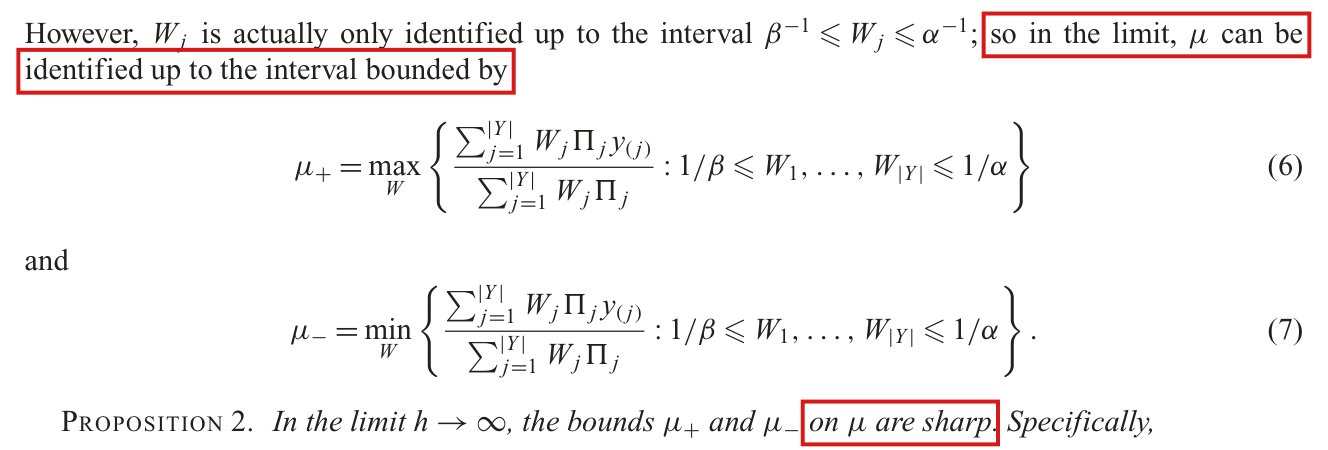
(S5) Outcome classes, class totals, the limiting optimisation problems [Section 3.2, p. 237 (PDF p. 3)]: 'Let $Y$ be the ordered set of distinct outcomes in $U$, so that $y_{(1)} < \cdots < y_{(|Y|)}$, with equivalence classes $\Upsilon_j \equiv \{i = 1, \ldots, N : y_i = y_{(j)}\}$. In the limit of the Brewer scaling, the probabilities $\pi_i$ can be identified up to units with identical outcomes: as $h \to \infty$, $(\sum_{\{i=1,\ldots,Nh : y_i = y_{(j)}\}} I_i)/(\sum_{i=1}^{Nh} I_i) \to \Pi_j/(\sum_{k=1}^{|Y|}\Pi_k)$ where $\Pi_j = \sum_{i\in\Upsilon_j}\pi_i$. Since $\pi_i \geqslant \alpha > 0$ for all $i$, $Y$ is identified in the limit. If $W_j \equiv |\Upsilon_j|/\Pi_j$ is known for all $j = 1, \ldots, |Y|$, then $\mu$ is identified: $\mu = \dfrac{\sum_{j=1}^{|Y|} W_j\Pi_j y_{(j)}}{\sum_{j=1}^{|Y|} W_j\Pi_j} = \dfrac{\sum_{j=1}^{|Y|} W_j \frac{\Pi_j}{\sum_{k=1}^{|Y|}\Pi_k} y_{(j)}}{\sum_{j=1}^{|Y|} W_j\frac{\Pi_j}{\sum_{k=1}^{|Y|}\Pi_k}}$. However, $W_j$ is actually only identified up to the interval $\beta^{-1} \leqslant W_j \leqslant \alpha^{-1}$; so in the limit, $\mu$ can be identified up to the interval bounded by $\mu_+ = \max_W\left\{\dfrac{\sum_{j=1}^{|Y|} W_j\Pi_j y_{(j)}}{\sum_{j=1}^{|Y|} W_j\Pi_j} : 1/\beta \leqslant W_1, \ldots, W_{|Y|} \leqslant 1/\alpha\right\}$ (6) and $\mu_- = \min_W\left\{\dfrac{\sum_{j=1}^{|Y|} W_j\Pi_j y_{(j)}}{\sum_{j=1}^{|Y|} W_j\Pi_j} : 1/\beta \leqslant W_1, \ldots, W_{|Y|} \leqslant 1/\alpha\right\}$. (7)'
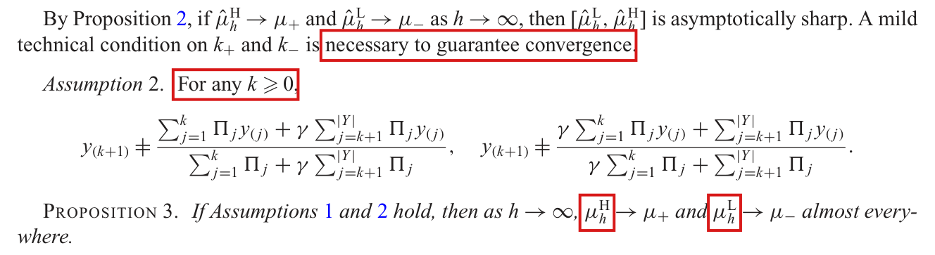
(S6) Assumption 2 [Section 3.2, p. 238 (PDF p. 4)], preceded by: 'By Proposition 2, if $\hat\mu^{\mathrm H}_h \to \mu_+$ and $\hat\mu^{\mathrm L}_h \to \mu_-$ as $h \to \infty$, then $[\hat\mu^{\mathrm L}_h, \hat\mu^{\mathrm H}_h]$ is asymptotically sharp. A mild technical condition on $k_+$ and $k_-$ is necessary to guarantee convergence.' 'Assumption 2. For any $k \geqslant 0$, $y_{(k+1)} \neq \dfrac{\sum_{j=1}^{k}\Pi_j y_{(j)} + \gamma\sum_{j=k+1}^{|Y|}\Pi_j y_{(j)}}{\sum_{j=1}^{k}\Pi_j + \gamma\sum_{j=k+1}^{|Y|}\Pi_j}$, $\quad y_{(k+1)} \neq \dfrac{\gamma\sum_{j=1}^{k}\Pi_j y_{(j)} + \sum_{j=k+1}^{|Y|}\Pi_j y_{(j)}}{\gamma\sum_{j=1}^{k}\Pi_j + \sum_{j=k+1}^{|Y|}\Pi_j}$.'
(S7) Reading conventions; these are not printed. They are the ones the validators fixed (validated.json, natural_reading fields) and every target uses them. (a) $n \geqslant 1$, $|Y| \geqslant 1$, and an empty sum is $0$. (b) A rule of the form 'the smallest nonnegative integer $k$ that satisfies [...] $y_{k+1}$' ranges over the integers $0 \leqslant k \leqslant n-1$, the only $k$ for which $y_{k+1}$ is defined; likewise $0 \leqslant k \leqslant |Y|-1$ for a rule in $y_{(k+1)}$ and for Assumption 2. (c) The objective of (2)-(3) is unchanged when $w$ is multiplied by a positive constant, so with $u = \beta w$ the box $[1/\beta, 1/\alpha]^n$ becomes $[1, \gamma]^n$. For $0 \leqslant k \leqslant n$ write $F^{\mathrm H}_k = \{\sum_{i=1}^{k} y_i + \gamma\sum_{i=k+1}^{n} y_i\}/\{k + \gamma(n-k)\}$ and $F^{\mathrm L}_k = \{\gamma\sum_{i=1}^{k} y_i + \sum_{i=k+1}^{n} y_i\}/\{\gamma k + (n-k)\}$: these are the values of $w'y/(w'1_n)$ at the threshold vectors $w^{k}$ (first $k$ entries $1/\beta$, last $n-k$ entries $1/\alpha$; Appendix, p. 239) and (first $k$ entries $1/\alpha$, last $n-k$ entries $1/\beta$), respectively. The same holds with class totals: for $0 \leqslant k \leqslant |Y|$, $G^{+}_k = \dfrac{\sum_{j=1}^{k}\Pi_j y_{(j)} + \gamma\sum_{j=k+1}^{|Y|}\Pi_j y_{(j)}}{\sum_{j=1}^{k}\Pi_j + \gamma\sum_{j=k+1}^{|Y|}\Pi_j}$ and $G^{-}_k = \dfrac{\gamma\sum_{j=1}^{k}\Pi_j y_{(j)} + \sum_{j=k+1}^{|Y|}\Pi_j y_{(j)}}{\gamma\sum_{j=1}^{k}\Pi_j + \sum_{j=k+1}^{|Y|}\Pi_j}$ are the values of the objective of (6)-(7) at the threshold vectors (first $k$ entries $1/\beta$, rest $1/\alpha$) and (first $k$ entries $1/\alpha$, rest $1/\beta$). (d) $\Pi_j > 0$ for every $j$, because each class $\Upsilon_j$ is nonempty and $\pi_i \geqslant \alpha > 0$; hence every denominator in (6), (7) and in $G^{\pm}_k$ is positive. (e) In Section 3.2 the estimators $\hat\mu^{\mathrm H}_h$, $\hat\mu^{\mathrm L}_h$ are (2) and (3) computed from the pooled sample $S_h$ (all sampled units of the $h$ replicates); they are defined when $S_h$ is nonempty.
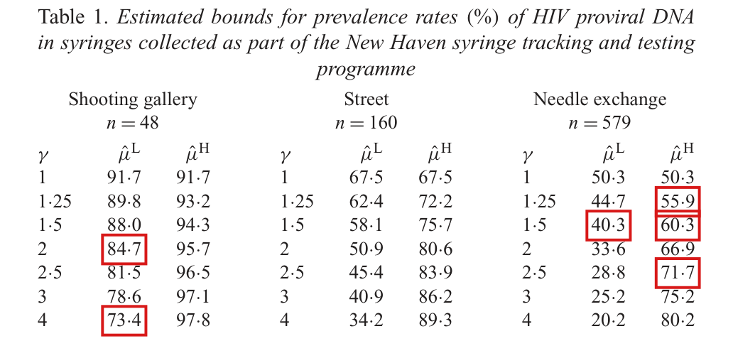
(S8) Transcription notes (checked on 420 dpi crops of the page images). (a) In (5) and in the dichotomous display the left-hand set is printed with $\pi_N$ (capital $N$), although $\hat\mu$ depends only on $\pi_1, \ldots, \pi_n$. (b) Proposition 3 prints $\mu^{\mathrm H}_h$ and $\mu^{\mathrm L}_h$ without hats; the sentence two lines above it and Assumption 1 print $\hat\mu^{\mathrm H}_h$, $\hat\mu^{\mathrm L}_h$. (c) In Proposition 2 the two second sums of the $\mu_-$ display are printed with lower limit $j = k_- - 1$; every other display of the paper has $k+1$ there. (d) The rule for $k^{\mathrm L}$ (p. 236) and the rule for $k_-$ (p. 238, directly below Table 1) are both printed with $\geqslant$; the rules for $k^{\mathrm H}$ and $k_+$ with $\leqslant$. (e) The supplement sets the superscripts H and L in italic and writes $\leq$, $\geq$; the article sets them upright and writes $\leqslant$, $\geqslant$.
Effective claim (source TeX): [Corrected statement; the printed sentences are: (p. 237) 'The proposed interval estimator yields asymptotically sharp bounds on $\mu$ itself under the scaling proposed by Brewer (1979) and articulated in Assumption 1.'; (p. 237) 'However, $W_j$ is actually only identified up to the interval $\beta^{-1} \leqslant W_j \leqslant \alpha^{-1}$; so in the limit, $\mu$ can be identified up to the interval bounded by' (6) and (7); (p. 237) 'PROPOSITION 2. In the limit $h \to \infty$, the bounds $\mu_+$ and $\mu_-$ on $\mu$ are sharp.' Sol's smallest repair, validated.json, P025-N002, as settled by the doubt check (validate/P025-N002/doubt/doubt.json): 'State: Conditional only on the limiting distribution q_j=Pi_j/sum_k Pi_k of outcomes among sampled units, and with original population size unrestricted, (6)-(7) are sharp lower and upper bounding endpoints, meaning the infimum and supremum of compatible finite-population means. Brewer replication supplies convergence; h-calibrated absolute count rates are not additional identification information. If original N or absolute Pi are retained, the interval is a valid outer bound and sharpness requires the corresponding integer/calibration conditions derived in artifact/derivation.md.']
PROPOSITION 2, first sentence (corrected). In the limit $h \to \infty$, conditional only on the limiting distribution $q_j = \Pi_j/\sum_{k=1}^{|Y|}\Pi_k$ of outcomes among sampled units, and with the size $N$ of the original population unrestricted, the bounds $\mu_+$ and $\mu_-$ on $\mu$ are sharp, in the sense that they are the supremum and the infimum of the means of the finite populations compatible with that information. If $N$, or the absolute limiting totals $\Pi_j$, are also retained, $[\mu_-, \mu_+]$ is a valid outer bound on $\mu$ that need not be sharp.
[Formal content, with every hypothesis; from validate/P025-N002/doubt/artifact/derivation.md, sections 2-4.] Fix $J \geqslant 1$, reals $y_{(1)} < \cdots < y_{(J)}$, numbers $0 < \alpha \leqslant \beta \leqslant 1$ with $\gamma = \beta/\alpha$, and $q = (q_1, \ldots, q_J)$ with every $q_j > 0$ and $\sum_j q_j = 1$. A compatible population is a finite population whose distinct outcomes are exactly $y_{(1)}, \ldots, y_{(J)}$, with $m_j \geqslant 1$ units of outcome $y_{(j)}$ (so $N = \sum_j m_j$ is not restricted), together with inclusion probabilities $\pi_i \in [\alpha, \beta]$ for its units such that $\Pi_j/\sum_k \Pi_k = q_j$ for every $j$, where $\Pi_j$ is the sum of $\pi_i$ over the units with outcome $y_{(j)}$. Its mean is $\mu(m) = \sum_j m_j y_{(j)}/\sum_j m_j$. Let $\mu_+(q)$ and $\mu_-(q)$ denote (6) and (7) with $\Pi_j$ replaced by $q_j$ (the objective of (6)-(7) is unchanged when all $\Pi_j$ are multiplied by one positive constant). Assume that at least one compatible population exists (this is automatic when $\gamma > 1$; when $\gamma = 1$ it holds exactly when $q$ is rational). Then: (a) [Outer bound.] For every compatible population, $W_j = m_j/\Pi_j \in [1/\beta, 1/\alpha]$ and $\mu(m) = \sum_j W_j\Pi_j y_{(j)}/\sum_j W_j\Pi_j$; hence $\mu_-(q) \leqslant \mu(m) \leqslant \mu_+(q)$. (b) [Sharpness.] $\inf \mu(m) = \mu_-(q)$ and $\sup \mu(m) = \mu_+(q)$, the infimum and supremum being over all compatible populations. (c) [The box in terms of population proportions.] Let $\mathcal{C}_\gamma(q) = \{r \in \mathbb{R}^J : r_j \geqslant 0,\ \sum_j r_j = 1,\ r_j q_k \leqslant \gamma\, r_k q_j \text{ for all } j, k\}$. The map $W \mapsto r$, $r_j = W_j q_j/\sum_k W_k q_k$, sends $[1/\beta, 1/\alpha]^J$ onto $\mathcal{C}_\gamma(q)$, so $\mu_+(q) = \max\{\sum_j r_j y_{(j)} : r \in \mathcal{C}_\gamma(q)\}$ and $\mu_-(q) = \min\{\sum_j r_j y_{(j)} : r \in \mathcal{C}_\gamma(q)\}$; and a vector $r$ is the vector of class proportions $(m_j/N)_j$ of some compatible population if and only if $r \in \mathcal{C}_\gamma(q)$ and $r$ has rational coordinates. (d) [Attainment.] $\mu_+(q)$ (respectively $\mu_-(q)$) is the mean of some compatible population if and only if the set of maximisers (respectively minimisers) of $\sum_j r_j y_{(j)}$ over $\mathcal{C}_\gamma(q)$ contains a vector with rational coordinates. (e) [Scope.] When the absolute totals $\Pi_j$ (the limits of $P_{h,j}$ in the Supplement) are retained with fixed $\alpha, \beta$, the compatible class sizes are the integers $m_j$ with $\Pi_j/\beta \leqslant m_j \leqslant \Pi_j/\alpha$, and additionally $\sum_j m_j = N$ when $N$ is known; (a) still holds, and (b) can fail (P025-T16).
: SAP.P025b.T15WholeStatement
Theorem: SAP.P025b.T15
Statement hash: c34a4227ba5bce2d3d51d0d7a678c482773b7d140fe9b94a6d4de97b9439bf9d
Statement definition: SAP.P025b.T15WholeStatement
Certificate. 20261104T182037Z
Declaration review: faithful; 2026-11-04T18:38:19Z; binding v2
Evidence scope: Certification checks formal proof objects. Statement fidelity is a model judgment. Author review is separate.
Proof dependencies: Independently extracted
Manifest annotation reconciliation: Effective use follows the source-bound dependency observation; original annotations are retained in the crosswalk.
AronowAudit.P025.box_proportion_image: observed used
AronowAudit.P025.box_proportions_in_region: observed used
AronowAudit.P025.class_proportion_mean: observed used
AronowAudit.P025.class_proportions_rational: observed used
AronowAudit.P025.compatible_endpoints_mem_closure: observed used
AronowAudit.P025.compatible_mean_iff_rational_region: observed used
AronowAudit.P025.compatible_proportions_iff_rational_region: observed used
AronowAudit.P025.mean_weight_proportions: observed used
AronowAudit.P025.proportion_region_mean_image: observed used
AronowAudit.P025.proportion_region_positive: observed used
AronowAudit.P025.rational_proportions_have_sizes: observed used
AronowAudit.P025.region_has_box_weights: observed used
AronowAudit.P025.region_mean_mem_closure: observed used
AronowAudit.P025.shares_sharp_endpoints: observed used
AronowAudit.P025.weight_proportions_scale_mass: observed used
AronowAudit.P025.weight_proportions_scale_weights: observed used
Source and evidence metadata · sap-2026-11-08-assured-release