Assumptions and verification
Claim revision: catalog:c814dd867397421dd0cfb46392d0ac0514e272a9888065a58b1145936c8703d4
Standing assumptions: Finite-population, design-based potential-outcomes setting (the Neyman-Rubin model): potential outcomes and covariates are fixed and the only randomness is the assignment of units to treatment and control. Transcribed from the page images.
(S1) Section 3, pp. 137-138 (PDF pp. 3-4): 'Define a binary treatment indicator $T_i$ for units $i = 1,2,\ldots,N$ such that $T_i = 1$ when unit $i$ receives the treatment and $T_i = 0$ otherwise. If the stable unit treatment value assumption [16] holds, let $Y_{1i}$ be the potential outcome if unit $i$ is exposed to the treatment, and let $Y_{0i}$ be the potential outcome if unit $i$ is not exposed to the treatment. The observed outcome $Y_i$ may be expressed as a function of the potential outcomes and the treatment: $Y_i = T_iY_{1i} + (1-T_i)Y_{0i}$. [1] The causal effect of the treatment on unit $i$, $\tau_i$, is defined as the difference between the two potential outcomes for unit $i$: $\tau_i \equiv Y_{1i} - Y_{0i}$. [2] The ATE, denoted by $\Delta$, is defined as the average value of $\tau_i$ for all units $i$. In the Neyman-Rubin model, the only random component is the allocation of units to treatment and control groups.' Eq. [3]: $\Delta = \frac{\sum_{i=1}^{N}\tau_i}{N} = \frac{\sum_{i=1}^{N}(Y_{1i}-Y_{0i})}{N} = \frac{1}{N}\left[\sum_{i=1}^{N}Y_{1i} - \sum_{i=1}^{N}Y_{0i}\right] = \frac{1}{N}\left[Y_1^T - Y_0^T\right]$, 'where $Y_1^T$ is the sum of the potential outcomes if in the treatment condition and $Y_0^T$ is the sum of potential outcomes if in the control condition.' Eq. [4]: $\widehat{\Delta} = \frac{1}{N}\left[\widehat{Y_1^T} - \widehat{Y_0^T}\right]$, 'where $\widehat{Y_1^T}$ is the estimated sum of potential outcomes under treatment and $\widehat{Y_0^T}$ is the estimated sum of potential outcomes under control.' Footnote 2 (p. 138): 'This assumption is made without loss of generality; multiple discrete treatments (or equivalently, some units not being sampled into either treatment or control) are easily accommodated in this framework. All instances of $(1 - T_i)$ in the text may be replaced by $C_i$, an indicator variable for whether or not unit $i$ receives the control, with one exception to be noted in Section 6.'
(S2) p. 138 (PDF p. 4): 'Formally, the bias of an estimator is the difference between the expected value of the estimator and the true parameter of interest; an estimator is unbiased if this difference is equal to zero. If the estimators $\widehat{Y_0^T}$ and $\widehat{Y_1^T}$ are unbiased, the corresponding estimator of $\Delta$ is also unbiased since $\mathrm{E}[\widehat{\Delta}] = \frac{1}{N}\left[\mathrm{E}[\widehat{Y_1^T}] - \mathrm{E}[\widehat{Y_0^T}]\right] = \frac{1}{N}\left[Y_1^T - Y_0^T\right] = \Delta$.' [5]
(S3) Section 4, p. 138 (PDF p. 4): 'Define $N$ as the number of units in the study, $\pi_{1i}$ as the probability that unit $i$ is selected into treatment, and $\pi_{0i}$ as the probability that unit $i$ is selected into control. We assume that, $\forall i$, $\pi_{1i} > 0$ and $\pi_{0i} > 0$, or that there is a nonzero probability that each unit will be selected into treatment and that there is a nonzero probability that each unit will be selected into control. (When all units are assigned to either treatment or control, $\pi_{0i} + \pi_{1i} = 1$.)'
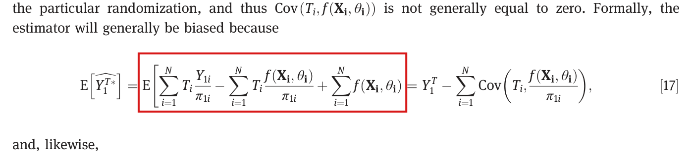
(S4) Section 5, pp. 140-141 (PDF pp. 6-7): eqs. [13]-[14], $\widehat{Y_1^{T*}} = \sum_{i=1}^{N}\left[T_i\frac{Y_{1i}}{\pi_{1i}} - T_i\frac{f(\mathbf{X_i},\theta_{\mathbf{i}})}{\pi_{1i}} + f(\mathbf{X_i},\theta_{\mathbf{i}})\right]$ and $\widehat{Y_0^{T*}} = \sum_{i=1}^{N}\left[(1-T_i)\frac{Y_{0i}}{\pi_{0i}} - (1-T_i)\frac{f(\mathbf{X_i},\theta_{\mathbf{i}})}{\pi_{0i}} + f(\mathbf{X_i},\theta_{\mathbf{i}})\right]$, 'where $f(.)$ is a predetermined real-valued function of pretreatment covariate vector $\mathbf{X_i}$ and of parameter vector $\theta_{\mathbf{i}}$'; eq. [15], $\widehat{\Delta_G} = \frac{1}{N}\left(\widehat{Y_1^{T*}} - \widehat{Y_0^{T*}}\right)$; eq. [16], $\widehat{\Delta_G} = \widehat{\Delta_{HT}} - \frac{1}{N}\left(\sum_{i=1}^{N}T_i\frac{f(\mathbf{X_i},\theta_{\mathbf{i}})}{\pi_{1i}} - \sum_{i=1}^{N}(1-T_i)\frac{f(\mathbf{X_i},\theta_{\mathbf{i}})}{\pi_{0i}}\right)$.
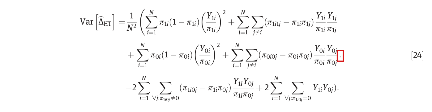
(S5) Section 6.1, p. 143 (PDF p. 9): '$\pi_{1i1j}$ is the probability that units $i$ and $j$ are jointly included in the treatment group'; '$\pi_{0i0j}$ is the probability that units $i$ and $j$ are jointly included in the control group'; '$\pi_{1i0j}$ is the joint probability that unit $i$ will be in the treatment group and unit $j$ will be in the control group.'
(S6) Section 6.2, pp. 143-144 (PDF pp. 9-10): 'When $f(\mathbf{X_i},\theta_{\mathbf{i}})$ is constant, we may simply redefine the outcome variable, $U_i = Y_i - f(\mathbf{X_i},\theta_{\mathbf{i}})$. It follows that $U_{0i} = Y_{0i} - f(\mathbf{X_i},\theta_{\mathbf{i}})$ and $U_{1i} = Y_{1i} - f(\mathbf{X_i},\theta_{\mathbf{i}})$.' and 'As we proceed, for notational clarity, we use $Y_i$ as the outcome measure, noting that the variances derived will also apply to the generalized difference estimator if $U_i$ is substituted for $Y_i$ (along with both associated potential outcomes) and $f(\mathbf{X_i},\theta_{\mathbf{i}})$ is constant.'
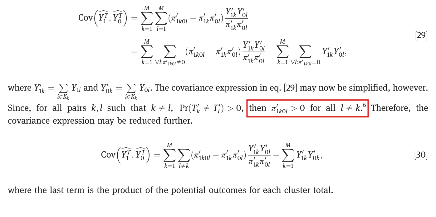
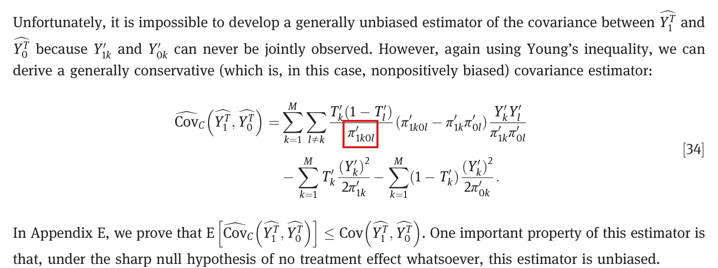
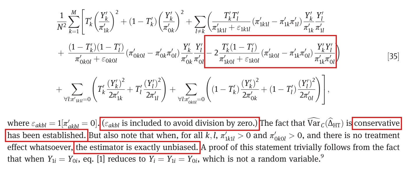
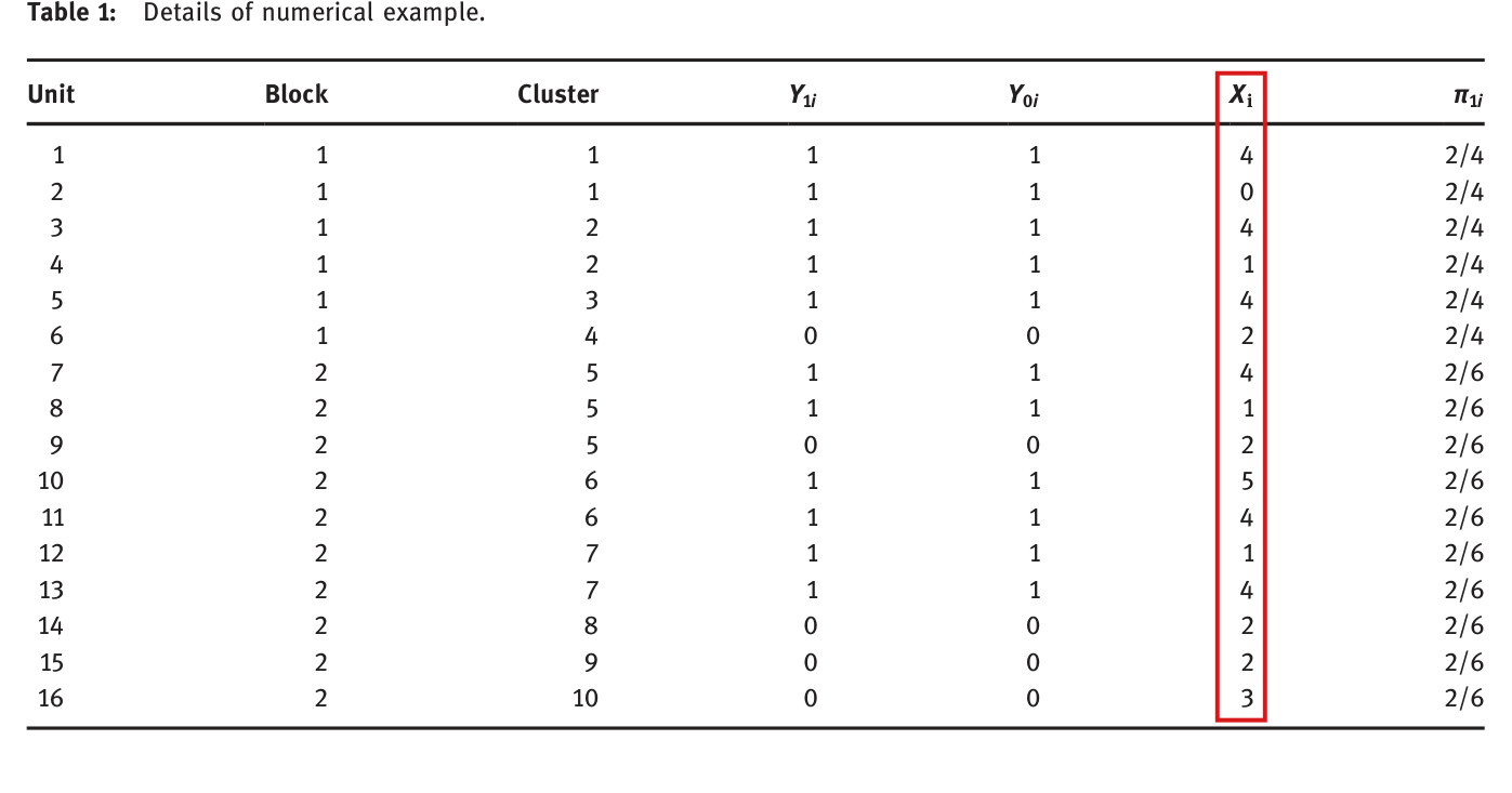
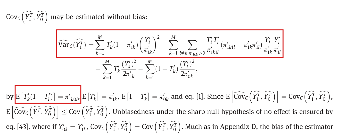
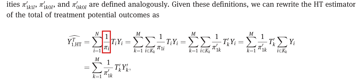
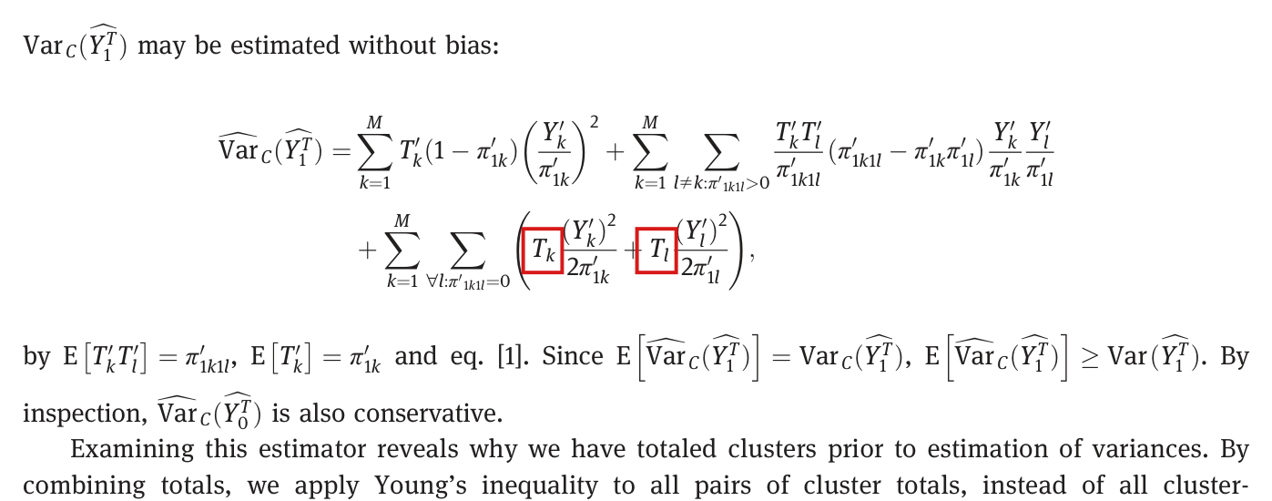
(S7) Section 6.3, pp. 144-145 (PDF pp. 10-11), cluster totals: 'Note that if, for some units $i,j$, $\Pr(T_i \neq T_j) = 0$, then the total estimators may be equivalently rewritten. Define $K_k \in \mathbf{K}$ as the set of unit indices $i$ that satisfy $T_i = T'_k$, where $T'_k$ is indexed over all $|\mathbf{K}|$ unique random variables in $\{T_i : i = (1,2,\ldots,N)\}$. Define $\pi'_{1k}$ as the value of $\pi_{1i}, \forall i \in K_k$, $\pi'_{0k}$ as the value of $\pi_{0i}, \forall i \in K_k$. Joint probabilities $\pi'_{1k1l}$, $\pi'_{1k0l}$, and $\pi'_{0k0l}$ are defined analogously.' With '$Y'_k = \sum_{i \in K_k} Y_i$' (p. 144) and '$Y'_{1k} = \sum_{i \in K_k} Y_{1i}$ and $Y'_{0k} = \sum_{i \in K_k} Y_{0i}$' (p. 145). The sums over clusters run over $k = 1,\ldots,M$.
(S8) Section 6.4, p. 145 (PDF p. 11): 'Our goal is now to derive conservative variance estimators: although not unbiased, these estimators are guaranteed to have a nonnegative bias.' Footnote 7: 'Although the variance estimator is nonnegatively biased, the associated standard errors may not be (due to Jensen's inequality) and any particular draw may be above or below the true value of the variance due to sampling variability.'
Reading conventions used in every target below (they follow from (S1)-(S7) in the two-arm case that the paper works in; stated here for the formalizer and flagged as conventions, not quotations): the assignment vector $(T_1,\ldots,T_N)$ has an arbitrary probability distribution on $\{0,1\}^N$ (a finite sample space), and all expectations, variances and covariances are taken over it; every unit is assigned to treatment or control, so $\pi_{1i} = \Pr(T_i = 1)$, $\pi_{0i} = \Pr(T_i = 0) = 1 - \pi_{1i}$, $\pi_{1i1j} = \Pr(T_i = 1, T_j = 1)$, $\pi_{0i0j} = \Pr(T_i = 0, T_j = 0)$, $\pi_{1i0j} = \Pr(T_i = 1, T_j = 0)$, hence $\pi_{1i1i} = \pi_{1i}$, $\pi_{0i0i} = \pi_{0i}$ and $\pi_{1i0i} = 0$, and likewise for the primed cluster quantities; the clusters $K_1,\ldots,K_M$ partition $\{1,\ldots,N\}$, $T_i = T'_k$ for every $i \in K_k$, and distinct clusters have distinct indicators, $\Pr(T'_k \neq T'_l) > 0$ for $k \neq l$; every double sum over $k, l$ (or $i, j$) is over ordered pairs; 'the sharp null hypothesis of no treatment effect whatsoever' means $Y_{1i} = Y_{0i}$ for every unit $i$.
Effective claim (source TeX): Printed statement refuted. p. 142 (PDF p. 8), Section 5.1: 'Following the basic logic of Williams [44], a second option, only possible in some studies, is to exploit the fact that for some units $i,j$, $T_i \perp\!\!\!\perp T_j$. Recall from (1) that $Y_i = T_iY_{1i} + (1-T_i)Y_{0i}$, where $Y_{1i}$ and $Y_{0i}$ are constants. Since the only stochastic component of $Y_i$ is $T_i$, then $T_i \perp\!\!\!\perp T_j$, and $T_i \perp\!\!\!\perp Y_j$. If $\theta_{\mathbf{i}}$ is a function of any or all of the elements of the set $\{Y_j : T_i \perp\!\!\!\perp T_j\}$ and no other random variables, then $T_i \perp\!\!\!\perp \theta_{\mathbf{i}}$. It follows that $T_i \perp\!\!\!\perp f(\mathbf{X_i},\theta_{\mathbf{i}})$ and therefore $\mathrm{Cov}(T_i,f(\mathbf{X_i},\theta_{\mathbf{i}})) = 0$.' Footnote 5 (p. 142): 'More formally and without loss of generality, let $f(\mathbf{X_i},\theta_{\mathbf{i}}) = f(\mathbf{X_i},g(\mathbf{Z},Y_j)) = f(\mathbf{X_i},g(\mathbf{Z},h(Y_{0j},Y_{1j},T_j)))$, where $\mathbf{Z}$ is a matrix of pretreatment covariates (that may or may not coincide with $\mathbf{X_j}$), $g(.)$ is an arbitrary function (e.g., the least squares fit), and $h(.)$ is the function implied by eq. [1]. Since only $T_j$ is a random variable, the random variable $f(\mathbf{X_i},\theta_{\mathbf{i}})$ equals some function $f'(T_j)$. $T_i \perp\!\!\!\perp T_j$ implies $T_i \perp\!\!\!\perp f'(T_j)$ (equivalently $T_i \perp\!\!\!\perp f(\mathbf{X_i},\theta_{\mathbf{i}})$) which, in turn, implies $\mathrm{Cov}(T_i,f(\mathbf{X_i},\theta_{\mathbf{i}})) = 0$.'
Counterexample A (the adjudicated validator's; six units, three treated and three control in every assignment; exact arithmetic). $N = 6$. The assignment $(T_1,\ldots,T_6)$ takes each of the four values $(0,1,0,1,0,1)$, $(0,1,1,0,1,0)$, $(1,0,0,1,1,0)$, $(1,0,1,0,0,1)$ with probability $1/4$; equivalently $T = (A, 1-A, B, 1-B, C, 1-C)$ with $A, B$ independent fair bits and $C = A + B - 2AB$. For every $i$: $Y_{0i} = 0$, $Y_{1i} = 1$ (so $Y_i = T_i$ and $\Delta = 1$), $X_i = 1$, and $f(X,\theta) = X\theta$. Let $Q(u,v) = u + v - 2uv$ and set $\theta_1 = Q(Y_3,Y_5)$, $\theta_2 = 1 - Q(Y_3,Y_5)$, $\theta_3 = Q(Y_1,Y_5)$, $\theta_4 = 1 - Q(Y_1,Y_5)$, $\theta_5 = Q(Y_1,Y_3)$, $\theta_6 = 1 - Q(Y_1,Y_3)$. Then:
(A-i) the paper's assumptions hold: $\pi_{1i} = \pi_{0i} = 1/2$ for every $i$; potential outcomes and covariates are fixed; $f$ is a fixed function;
(A-ii) the hypothesis of the printed statement holds for every $i$: $T_i \perp\!\!\!\perp T_j$ for every pair $i,j$ not of the form $\{1,2\}$, $\{3,4\}$, $\{5,6\}$ (all four joint cells have probability $1/4$), so $\{Y_j : T_1 \perp\!\!\!\perp T_j\} = \{Y_3,Y_4,Y_5,Y_6\}$, the same set for $i = 2$, $\{Y_1,Y_2,Y_5,Y_6\}$ for $i = 3,4$ and $\{Y_1,Y_2,Y_3,Y_4\}$ for $i = 5,6$; each $\theta_i$ is a function of two elements of the set for unit $i$ and of no other random variable;
(A-iii) the conclusions fail: $\theta_i = f(X_i,\theta_i) = T_i$ on every assignment, so $T_i$ is not independent of $\theta_i$ ($\Pr(T_i = 1, \theta_i = 1) = 1/2 \neq 1/4$) and $\mathrm{Cov}(T_i, f(X_i,\theta_i)) = 1/4 \neq 0$ for every $i$;
(A-iv) by eqs. [13]-[15], $\widehat{Y_1^{T*}} = 3$ and $\widehat{Y_0^{T*}} = 3$ on every assignment, so $\widehat{\Delta_G} = 0$ on every assignment and $\mathrm{E}[\widehat{\Delta_G}] - \Delta = -1$, in agreement with eq. [19] ($-\frac{1}{6}\cdot 6\cdot\frac{1}{4}\cdot(2+2)$), while $\widehat{\Delta_{HT}} = 1$ on every assignment.
Counterexample B (smaller; from the fresh readers, re-verified by the validators). $N = 3$; $(T_1,T_2,T_3)$ takes each of $(0,0,0)$, $(0,1,1)$, $(1,0,1)$, $(1,1,0)$ with probability $1/4$; $Y_{0i} = 0$, $Y_{1i} = 1$, $X_i = 1$, $f(X,\theta) = X\theta$. Every pair of assignments is independent and every $\pi_{1i} = 1/2$. (B-i) With $\theta_i = Q(Y_j,Y_k)$ for $\{j,k\} = \{1,2,3\}\setminus\{i\}$: $f(X_i,\theta_i) = T_i$, $\mathrm{Cov}(T_i,f(X_i,\theta_i)) = 1/4$, $\widehat{\Delta_G} = 0$ on every assignment, bias $-1$. (B-ii) With $\theta_1 = \theta_2 = 0$ and $\theta_3 = Y_1Y_2$: $\mathrm{Cov}(T_3, f(X_3,\theta_3)) = -1/8$ and $\mathrm{E}[\widehat{\Delta_G}] = 7/6$, bias $+1/6$.
: SAP.P026a.T4WholeStatement
Theorem: SAP.P026a.T4
Statement hash: 12bd005a0a1b349ebed28d6ac63711af784b3f9d4e9185aff82cd81dcc0aac79
Statement definition: SAP.P026a.T4WholeStatement
Certificate. 20261104T181503Z
Declaration review: faithful; 2026-11-04T18:59:04Z; binding v2
Evidence scope: Certification checks formal proof objects. Statement fidelity is a model judgment. Author review is separate.
Proof dependencies: Independently extracted
Source and evidence metadata · sap-2026-11-08-assured-release












My comment and the history of this entry