LLM-generated corrections to the published research of P. M. Aronow

Journal article P026

Corrections to: A Class of Unbiased Estimators of the Average Treatment Effect in Randomized Experiments

P. M. Aronow and Joel A. Middleton (2013). A Class of Unbiased Estimators of the Average Treatment Effect in Randomized Experiments. Journal of Causal Inference 1(1):135–154.

DOI
10.1515/jci-2012-0009
Audited edition
Journal of Causal Inference, 2013, 1(1):135–154; 20 pages in the audited file
SHA-256 of the audited file
0e4291aa2052b86d09b912b88fb5990d95a2eb50746686ebf30de0b12c3c1e89
Permanent address
https://pmaronow.github.io/llm-audit/works/P026/

Summary

The paper asks how to estimate the average treatment effect without bias in randomized experiments of any design, including clustered designs and designs with unequal probabilities. It proposes Horvitz–Thompson estimators, a generalized difference estimator that adjusts for covariates without bias when the predictions are uncorrelated with assignment, and conservative variance estimators. 8 entries are classified as errors (3 Moderate, 5 Minor), and 2 are clarity notes; 3 Moderate and 4 Minor errors are in the article, and 1 Minor error is in the help page of the companion ri package (P026-N004). One Moderate error is P026-E002: the variance estimator [35] is not conservative for every design, and becomes so when one term is added.

What was and was not checked

I checked the following points, which held up under the conditions stated.

  • Equations [1]–[8]: the definitions, the decomposition into totals, and the unbiasedness of the Horvitz–Thompson estimators of each total and of the average treatment effect when the assignment probabilities are known and positive.
  • Equation [11], that the Horvitz–Thompson estimator is the difference in means under complete randomization of units, and equation [12], that it need not be under complete randomization of clusters. In an exact example with unequal clusters the difference in means is biased and the Horvitz–Thompson estimator is not.
  • Equations [13]–[16]: the generalized difference estimator equals Δ^HT\widehat{\Delta}_{HT} minus the adjustment term.
  • Equations [17]–[19] and Appendix B: the bias identity and the sufficiency of Cov⁡(Ti,f(Xi,θi))=0\operatorname{Cov}(T_i,f(\mathbf{X}_i,\theta_i))=0, apart from the bracket of P026-N001. The identity [19] agrees with exact enumeration on 1150 random designs in which ff depends on the randomization.
  • Equations [20]–[30]: the variance expressions, apart from the misprints of P026-E005. Equation [24] equals the enumerated variance on 1150 random designs in exact arithmetic, and [30] holds for every design (see P026-E002).
  • Equation [31] is unbiased when all π1k1l′>0\pi'_{1k1l}>0. The Young bounds behind [32], [33] and Appendix D are correct, and these two estimators are conservative for the arm variances in every design.
  • Equation [35] equals N−2N^{-2} times ([32] ++ [33] −2 -2\,[34]). It is conservative, and exactly unbiased under the sharp null when every pair of clusters has positive probability of joint treatment and of joint control, in each of 936 random designs with π1k0l′>0\pi'_{1k0l}>0 for all k≠lk\ne l, and in the example of Section 7.
  • Appendix A (equation [38]) and Appendix C (equation [42]), line by line, under the assumption [41].
  • Table 1: 16 units, 10 clusters, two blocks, 90 equally likely randomizations, and probabilities 2/42/4 and 2/62/6. For distinct clusters, the smallest joint probabilities are π1k1l′=1/15\pi'_{1k1l}=1/15, π0k0l′=1/6\pi'_{0k0l}=1/6 and π1k0l′=1/6\pi'_{1k0l}=1/6.
  • Table 2, columns IPW, FE, HT and G (Prior): every entry agrees with a recalculation from Table 1 to the third decimal, with exact variances 353/1920353/1920 for HT and 233/2560233/2560 for G (Prior). Within each column of Table 2 the rows are consistent with one another: the variance is the square of the standard error, and the squared RMSE is the variance plus the squared bias, to rounding.
  • For the population of Table 1, G (Linear) and G (Logit) have mean zero, their variance estimators are unbiased, and their RMSE is lower than that of IPW, FE and FE (Cov.) (see P026-E003).
  • The cross-references to sections, equations and appendices, and the citation numbers other than the one in footnote 8.
  • In the ri package, genperms and genprobexact return the 90 randomizations and the probabilities of Table 1; estate with HT=TRUE and no X computes equation [8], and with Ypre it computes the difference estimator with fixed ff; and gendist reproduces the expectation and SE rows of the IPW, HT and G (Prior) columns of Table 2.

The following were not checked or not settled. I did not read the cited works, among them Aronow and Samii [46], Wood [45], Williams [44] and Middleton and Aronow [5]. Statements attributed to them were checked by derivation or enumeration, and what the paper says about consistency and about the outside literature was not compared with the cited works. The records of Godambe’s and of Horvitz and Thompson’s articles were consulted for their bibliographic details only. The RE (Cov.) column of Table 2 could not be settled, because the version of lme4 that the paper cites was unavailable for comparison. The available replication files do not include the commands and inputs behind Table 2, and the ri package does not implement the variance estimator [35], which was computed directly from the equation. That this audit records no further corrections is not a finding that the rest of the paper is correct.

Headline claims and related corrections

  1. The Horvitz-Thompson difference-of-totals estimator (eq. [8]) is unbiased for the finite-population ATE in any randomised experiment whose assignment probabilities are known and strictly between 0 and 1, whatever the clustering, the heterogeneity of probabilities, the dependence in assignment or the form of the effects.

    eqs. [5]-[8]; eqs. [11]-[12]; Table 2 column HT

  2. Under complete randomisation of units the HT estimator is the difference in means; under complete randomisation of clusters it need not be, and difference-in-means, IPW and regression estimators can be biased in clustered or unequal-probability designs or with covariate adjustment.

    eqs. [11], [12]; Table 2 columns IPW, FE, FE (Cov.)

    See P026-E003.

  3. The generalised difference estimator (eqs. [13]–[16]) gives unbiased covariate adjustment with any outcome model ff provided Cov⁡(Ti,f(Xi,θi))=0\operatorname{Cov}(T_i,f(\mathbf{X}_i,\theta_i))=0 for every ii. The paper states that this holds when θi\theta_i is fixed in advance or computed only from outcomes of units whose assignments are each independent of TiT_i.

    eqs. [13]-[19]; Appendix B (eqs. [39]-[40]); Section 5.1 and footnote 5; Table 2 columns G (Prior), G (Linear), G (Logit)

    See P026-E001, P026-N001, P026-N004.

  4. The HT estimator is not location invariant, whereas the generalised difference estimator is when the fitted function transforms with the outcome.

    Appendix A (eqs. [36]-[38]); Appendix C (eqs. [41]-[42])

  5. The paper gives closed-form expressions for the sampling variance of the HT estimator and, with fixed ff, of the generalised difference estimator, at unit level and at the level of cluster totals.

    eqs. [20]-[30]

    See P026-E002, P026-E005.

  6. The variance estimator of eq. [35] is conservative (nonnegatively biased) for any experimental design when ff is fixed, and is exactly unbiased under the sharp null when all pairs of clusters have positive probability of joint treatment and of joint control.

    eqs. [31]-[35]; Appendices D and E; footnote 9

    See P026-E002, P026-E004, P026-E005, P026-N002.

  7. In the 16-unit, 10-cluster, 2-block example under the sharp null, only the HT-based estimators are unbiased; the regression-based ATE and variance estimators are negatively biased; the covariate-adjusted HT-based estimators have lower RMSE than the regression-based ones; and the HT-based variance estimators are unbiased.

    Table 1; Table 2

    See P026-E003.

  8. Outcome modelling within the proposed class can improve precision while retaining unbiasedness under the stated restrictions.

    Section 5; Section 7 and Table 2

    See P026-E003, P026-A001.

Corrections

Moderate (3)

A real substantive error with limited reach.

A sufficient condition for fitting θi\theta_i from other units' outcomes while preserving unbiasedness is independence of TiT_i from the whole vector of assignments used in the fit; independence from each assignment separately does not suffice.

Section 5.1, second paragraph, and footnote 5, p. 142 (PDF p. 8)

See also under Formal statements (Lean): P026-T4, P026-T5, P026-T18

My comment on this entry

As printed

“If θi\theta_i is a function of any or all of the elements of the set {Yj:Ti⊥ ⁣ ⁣ ⁣⊥Tj}\colorbox{#ffe58a}{$\{Y_j:T_i\perp\!\!\!\perp T_j\}$} and no other random variables, then Ti⊥ ⁣ ⁣ ⁣⊥θiT_i\perp\!\!\!\perp\theta_i. It follows that Ti⊥ ⁣ ⁣ ⁣⊥f(Xi,θi)T_i\perp\!\!\!\perp f(\mathbf{X}_i,\theta_i) and therefore Cov⁡(Ti,f(Xi,θi))=0\operatorname{Cov}(T_i,f(\mathbf{X}_i,\theta_i))=0.5{}^{5}”

Footnote 5: “More formally and without loss of generality, let f(Xi,θi)=f(Xi,g(Z,Yj))=f(Xi,g(Z,h(Y0j,Y1j;Tj))))f(\mathbf{X}_i,\theta_i)=f(\mathbf{X}_i,g(\mathbf{Z},\colorbox{#ffe58a}{$Y_j$}))=f(\mathbf{X}_i,g(\mathbf{Z},\colorbox{#ffe58a}{$h(Y_{0j},Y_{1j};T_j)$}))), where Z\mathbf{Z} is a matrix of pretreatment covariates (that may or may not coincide with Xj\mathbf{X}_j), g(.)g(.) is an arbitrary function (e.g., the least squares fit), and h(.)h(.) is the function implied by eq. [1]. Since only TjT_j is a random variable, the random variable f(Xi,θi)f(\mathbf{X}_i,\theta_i) equals some function f′(Tj)f'(T_j). Ti⊥ ⁣ ⁣ ⁣⊥TjT_i\perp\!\!\!\perp T_j implies Ti⊥ ⁣ ⁣ ⁣⊥f′(Tj)T_i\perp\!\!\!\perp f'(T_j) (equivalently Ti⊥ ⁣ ⁣ ⁣⊥f(Xi,θi)T_i\perp\!\!\!\perp f(\mathbf{X}_i,\theta_i)) which, in turn, implies Cov⁡(Ti,f(Xi,θi))=0\operatorname{Cov}(T_i,f(\mathbf{X}_i,\theta_i))=0.”

The problem

The set {Yj:Ti⊥ ⁣ ⁣ ⁣⊥Tj}\{Y_j:T_i\perp\!\!\!\perp T_j\} is defined by the independence of TiT_i from each TjT_j separately. A parameter θi\theta_i fitted from several of these outcomes is a function of several assignments jointly, and TiT_i can be independent of each of them and still depend on the vector they form. The conclusion Ti⊥ ⁣ ⁣ ⁣⊥θiT_i\perp\!\!\!\perp\theta_i does not follow from the stated premise, and neither does Cov⁡(Ti,f(Xi,θi))=0\operatorname{Cov}(T_i,f(\mathbf{X}_i,\theta_i))=0. Footnote 5 treats a fit that uses one outcome YjY_j, in which case θi\theta_i is a function of TjT_j alone, and for that case its argument is correct. The reduction to that case is not without loss of generality when the fit uses several outcomes.

When the premise holds only pairwise, the generalized difference estimator can be biased. In the design with six units described below, every randomization has three treated units and three controls, every outcome used in a fit belongs to the printed set, the estimate is 00 in every randomization, and the average treatment effect is 11.

Evidence an exact counterexample

This correction rests on an exact counterexample, computed in rational arithmetic, and on a derivation of the corrected condition.

Counterexample. Let N=6N=6, and let the randomization (T1,…,T6)(T_1,\ldots,T_6) take the four values 010101010101, 011010011010, 100110100110, 101001101001 with probability 1/41/4 each. Equivalently, T=(A,1−A,B,1−B,C,1−C)T=(A,1-A,B,1-B,C,1-C), where AA and BB are independent fair bits and C=A+B−2ABC=A+B-2AB. Every unit has π1i=π0i=1/2\pi_{1i}=\pi_{0i}=1/2. For two units in different pairs among {1,2}\{1,2\}, {3,4}\{3,4\}, {5,6}\{5,6\}, each of the four joint outcomes of their assignments has probability 1/41/4, and the two assignments are independent. The printed set then contains Y3,Y4,Y5,Y6Y_3,Y_4,Y_5,Y_6 for units 1 and 2, Y1,Y2,Y5,Y6Y_1,Y_2,Y_5,Y_6 for units 3 and 4, and Y1,Y2,Y3,Y4Y_1,Y_2,Y_3,Y_4 for units 5 and 6. The assignment T5T_5 is not independent of the pair (T1,T3)(T_1,T_3): Pr⁡(T5=0,T1=0,T3=0)=1/4\Pr(T_5=0,T_1=0,T_3=0)=1/4, while Pr⁡(T5=0)Pr⁡(T1=0,T3=0)=1/8\Pr(T_5=0)\Pr(T_1=0,T_3=0)=1/8.

Let Y0i=0Y_{0i}=0, Y1i=1Y_{1i}=1 and Xi=1X_i=1 for every unit, and let f(X,θ)=Xθf(X,\theta)=X\theta. Then Yi=TiY_i=T_i and Δ=1\Delta=1. Let Q(u,v)=u+v−2uvQ(u,v)=u+v-2uv, and fix the rules

θ1=Q(Y3,Y5),θ3=Q(Y1,Y5),θ5=Q(Y1,Y3),θ2=1−Q(Y3,Y5),θ4=1−Q(Y1,Y5),θ6=1−Q(Y1,Y3).\begin{aligned} \theta_1&=Q(Y_3,Y_5),&\qquad\theta_3&=Q(Y_1,Y_5),&\qquad\theta_5&=Q(Y_1,Y_3),\\ \theta_2&=1-Q(Y_3,Y_5),&\qquad\theta_4&=1-Q(Y_1,Y_5),&\qquad\theta_6&=1-Q(Y_1,Y_3). \end{aligned}

Each rule uses two outcomes of the printed set for its unit and no other random variable. Since Q(B,C)=AQ(B,C)=A, Q(A,C)=BQ(A,C)=B and Q(A,B)=CQ(A,B)=C, I have f(Xi,θi)=θi=Tif(X_i,\theta_i)=\theta_i=T_i for every unit in every randomization. Hence Cov⁡(Ti,f(Xi,θi))=1/2−1/4=1/4\operatorname{Cov}(T_i,f(X_i,\theta_i))=1/2-1/4=1/4 for all ii. Substituting π1i=π0i=1/2\pi_{1i}=\pi_{0i}=1/2 and f(Xi,θi)=Tif(X_i,\theta_i)=T_i into [13] and [14], I obtain

Y1T∗^=∑i=16(2Ti−2Ti2+Ti)=3,Y0T∗^=∑i=16(−2(1−Ti)Ti+Ti)=3,\widehat{Y_1^{T*}}=\sum_{i=1}^{6}\left(2T_i-2T_i^2+T_i\right)=3,\qquad\widehat{Y_0^{T*}}=\sum_{i=1}^{6}\left(-2(1-T_i)T_i+T_i\right)=3,

so that Δ^G=(3−3)/6=0\widehat{\Delta}_G=(3-3)/6=0 in every randomization, and the bias is −1-1. By equation [19], the bias is again −(1/6)⋅6⋅(1/4)⋅(2+2)=−1-(1/6)\cdot 6\cdot(1/4)\cdot(2+2)=-1. The Horvitz–Thompson estimate equals 11 in every randomization.

The four randomizations of the design with six units, each with probability 1/41/4. The true totals are Y1T=6Y_1^T=6 and Y0T=0Y_0^T=0, and Δ=1\Delta=1.
RandomizationPredictions f(Xi,θi)f(X_i,\theta_i), i=1,…,6i=1,\ldots,6Y1T∗^\widehat{Y_1^{T*}}Y0T∗^\widehat{Y_0^{T*}}Δ^G\widehat{\Delta}_GΔ^HT\widehat{\Delta}_{HT}
010101010101(0,1,0,1,0,1)(0,1,0,1,0,1)33330011
011010011010(0,1,1,0,1,0)(0,1,1,0,1,0)33330011
100110100110(1,0,0,1,1,0)(1,0,0,1,1,0)33330011
101001101001(1,0,1,0,0,1)(1,0,1,0,0,1)33330011

Derivation of the corrected condition. Fix a set JiJ_i of units, and let Vi=(Tj)j∈JiV_i=(T_j)_{j\in J_i}. Suppose that TiT_i is independent of ViV_i and that θi\theta_i depends only on (Yj)j∈Ji(Y_j)_{j\in J_i} and on fixed quantities. Since the potential outcomes are fixed, equation [1] implies that f(Xi,θi)=Hi(Vi)f(\mathbf{X}_i,\theta_i)=H_i(V_i) for a fixed function HiH_i. For a∈{0,1}a\in\{0,1\} and any set DD of values,

Pr⁡(Ti=a, Hi(Vi)∈D)=∑v:Hi(v)∈DPr⁡(Ti=a, Vi=v)=Pr⁡(Ti=a)∑v:Hi(v)∈DPr⁡(Vi=v)=Pr⁡(Ti=a)Pr⁡(Hi(Vi)∈D).\begin{aligned} \Pr(T_i=a,\,H_i(V_i)\in D)&=\sum_{v:H_i(v)\in D}\Pr(T_i=a,\,V_i=v)\\ &=\Pr(T_i=a)\sum_{v:H_i(v)\in D}\Pr(V_i=v)\\ &=\Pr(T_i=a)\Pr(H_i(V_i)\in D). \end{aligned}

The sums are finite. Hence TiT_i and f(Xi,θi)f(\mathbf{X}_i,\theta_i) are independent, and their covariance is zero. Equation [19] then implies that Δ^G\widehat{\Delta}_G is unbiased.

What survives

The Horvitz–Thompson estimator, the definitions [13]–[16], the bias identity [19], and the sufficient condition Cov⁡(Ti,f(Xi,θi))=0\operatorname{Cov}(T_i,f(\mathbf{X}_i,\theta_i))=0 with its proof in Appendix B are unaffected. The two fitting examples in Section 5.1 satisfy the corrected condition. These are designs in which units are assigned independently and the fit for unit ii leaves out unit ii, and designs in which blocks are randomized independently and the fit leaves out the block of unit ii, as in Section 7. Under the sharp null the observed outcomes are fixed, and so is any fit from them. A prediction that is additive in the outcomes with fixed coefficients, f(Xi,θi)=ai+∑jbijYjf(\mathbf{X}_i,\theta_i)=a_i+\sum_jb_{ij}Y_j, has zero covariance with TiT_i under the printed pairwise rule, because Cov⁡(Ti,Yj)=(Y1j−Y0j)Cov⁡(Ti,Tj)=0\operatorname{Cov}(T_i,Y_j)=(Y_{1j}-Y_{0j})\operatorname{Cov}(T_i,T_j)=0. What changes is the general rule for an arbitrary fit: the stronger premise gives a valid guarantee of unbiasedness and excludes designs such as the one above.

Corrected

“If, for a set JiJ_i of units fixed before the randomization, the assignment TiT_i is independent of the vector (Tj)j∈Ji\colorbox{#ffe58a}{$(T_j)_{j\in J_i}$}, and θi\theta_i is a function of the elements of the set {Yj:j∈Ji}\colorbox{#ffe58a}{$\{Y_j:j\in J_i\}$}, of fixed pretreatment quantities and of no other random variables, then Ti⊥ ⁣ ⁣ ⁣⊥θiT_i\perp\!\!\!\perp\theta_i. It follows that Ti⊥ ⁣ ⁣ ⁣⊥f(Xi,θi)T_i\perp\!\!\!\perp f(\mathbf{X}_i,\theta_i) and therefore Cov⁡(Ti,f(Xi,θi))=0\operatorname{Cov}(T_i,f(\mathbf{X}_i,\theta_i))=0.”

Footnote 5: “More formally, let

f(Xi,θi)=f(Xi,g(Z,(Yj)j∈Ji))=f(Xi,g(Z,(h(Y0j,Y1j;Tj))j∈Ji)),f(\mathbf{X}_i,\theta_i)=f\left(\mathbf{X}_i,g\left(\mathbf{Z},\colorbox{#ffe58a}{$\displaystyle (Y_j)_{j\in J_i}$}\right)\right)=f\left(\mathbf{X}_i,g\left(\mathbf{Z},\colorbox{#ffe58a}{$\displaystyle (h(Y_{0j},Y_{1j};T_j))_{j\in J_i}$}\right)\right),

where Z\mathbf{Z} is a matrix of pretreatment covariates, g(.)g(.) is an arbitrary function (e.g., the least squares fit), and h(.)h(.) is the function implied by eq. [1]. Since only the TjT_j are random variables, the random variable f(Xi,θi)f(\mathbf{X}_i,\theta_i) equals some function f′((Tj)j∈Ji)\colorbox{#ffe58a}{$f'((T_j)_{j\in J_i})$}. Independence of TiT_i and the vector (Tj)j∈Ji(T_j)_{j\in J_i} implies Ti⊥ ⁣ ⁣ ⁣⊥f′((Tj)j∈Ji)T_i\perp\!\!\!\perp f'((T_j)_{j\in J_i}) (equivalently Ti⊥ ⁣ ⁣ ⁣⊥f(Xi,θi)T_i\perp\!\!\!\perp f(\mathbf{X}_i,\theta_i)) which, in turn, implies Cov⁡(Ti,f(Xi,θi))=0\operatorname{Cov}(T_i,f(\mathbf{X}_i,\theta_i))=0.”

The premise can be replaced by a direct check that Cov⁡(Ti,f(Xi,θi))=0\operatorname{Cov}(T_i,f(\mathbf{X}_i,\theta_i))=0 for all ii. It also suffices that TiT_i be independent of the vector of observed outcomes (Yj)j∈Ji(Y_j)_{j\in J_i}.

Crop of six lines of the paragraph beginning 'Following the basic logic of Williams'. Red boxes mark the words 'any', 'or all of the elements of the set of Y-j such that T-i is independent of T-j', and 'then T-i is independent of theta-i'.
Section 5.1, second paragraph, p. 142 (PDF p. 8). The marked words define the admissible outcomes by independence of TiT_i from each TjT_j separately and conclude that TiT_i is independent of θi\theta_i.
Crop of the four lines of footnote 5. Red boxes mark the words 'without loss of generality,', the expression 'f of X-i and g of Z and Y-j', which has a single outcome Y-j as its argument, and the step 'T-i independent of T-j implies T-i independent of f-prime of T-j'.
Footnote 5, p. 142 (PDF p. 8). The argument is written for a single outcome YjY_j and is said to lose no generality.
My comment and the history of this entry

Yes, agreed. This was informal about pairwise vs joint independence.

  1. Classification before my review (the classification when the audit was first completed, before I reviewed it): Moderate error.
  2. I commented.
  3. Independent evaluation. No change was needed. The independent check upheld the six-unit counterexample, and the entry remains a Moderate error.

Two distinct clusters need not have π1k0l′>0\pi'_{1k0l}>0; when π1k0l′=0\pi'_{1k0l}=0 for some k≠lk\ne l, the covariance estimator [34] is undefined and the variance estimator [35] can be biased downward, also under the sharp null. Adding one term to [35] makes it conservative for every design.

Section 6.3, sentence between equations [29] and [30], p. 145 (PDF p. 11); equation [34], p. 146 (PDF p. 12); equation [35], the sentences after it and footnote 9, p. 147 (PDF p. 13); Appendix E, p. 152 (PDF p. 18); p. 137 (PDF p. 3)

See also under Formal statements (Lean): P026-T1, P026-T2, P026-T3, P026-T8, P026-T17, P026-T24

As printed

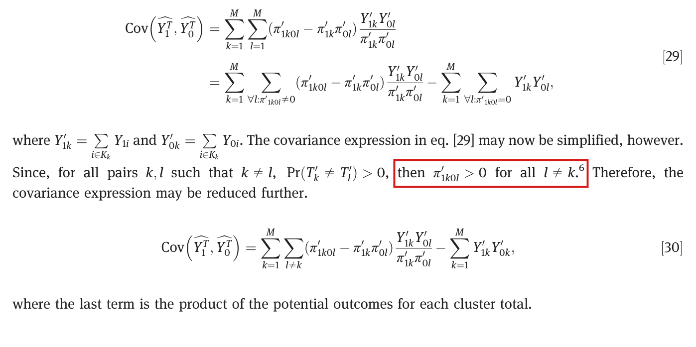
p. 145: “Since, for all pairs k,lk,l such that k≠lk\ne l, Pr⁡(Tk′≠Tl′)>0\Pr(T'_k\ne T'_l)>0, then π1k0l′>0\colorbox{#ffe58a}{$\pi'_{1k0l}>0$} for all l≠k\colorbox{#ffe58a}{$l\ne k$}.6{}^{6} Therefore, the covariance expression may be reduced further.”

p. 146, equation [34]:

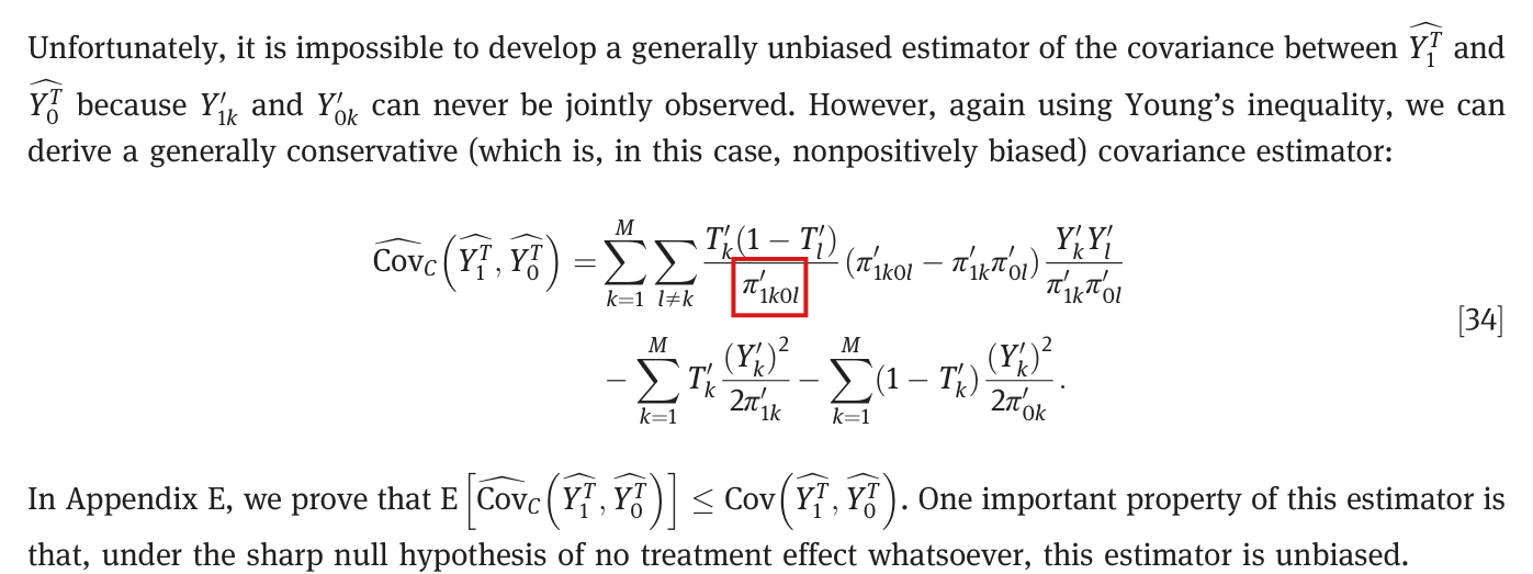
Cov⁡^C(Y1T^,Y0T^)=∑k=1M∑l≠kTk′(1−Tl′)π1k0l′(π1k0l′−π1k′π0l′)Yk′Yl′π1k′π0l′−∑k=1MTk′(Yk′)22π1k′−∑k=1M(1−Tk′)(Yk′)22π0k′.\begin{aligned} \widehat{\operatorname{Cov}}_C\left(\widehat{Y_1^T},\widehat{Y_0^T}\right)={}&\sum_{k=1}^{M}\sum_{l\ne k}\frac{T'_k(1-T'_l)}{\colorbox{#ffe58a}{$\displaystyle \pi'_{1k0l}$}}(\pi'_{1k0l}-\pi'_{1k}\pi'_{0l})\frac{Y'_kY'_l}{\pi'_{1k}\pi'_{0l}}\\ &-\sum_{k=1}^{M}T'_k\frac{(Y'_k)^2}{2\pi'_{1k}}-\sum_{k=1}^{M}(1-T'_k)\frac{(Y'_k)^2}{2\pi'_{0k}}. \end{aligned}

p. 147, equation [35]:

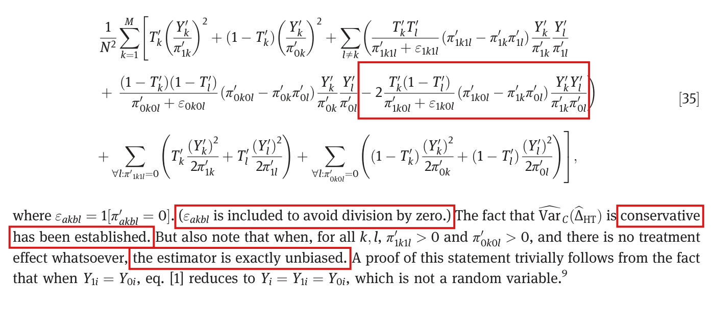
Var⁡^C(Δ^HT)=1N2∑k=1M[Tk′(Yk′π1k′)2+(1−Tk′)(Yk′π0k′)2+∑l≠k(Tk′Tl′π1k1l′+ε1k1l(π1k1l′−π1k′π1l′)Yk′Yl′π1k′π1l′+(1−Tk′)(1−Tl′)π0k0l′+ε0k0l(π0k0l′−π0k′π0l′)Yk′Yl′π0k′π0l′−2Tk′(1−Tl′)π1k0l′+ε1k0l(π1k0l′−π1k′π0l′)Yk′Yl′π1k′π0l′)+∑∀l:π1k1l′=0(Tk′(Yk′)22π1k′+Tl′(Yl′)22π1l′)+∑∀l:π0k0l′=0((1−Tk′)(Yk′)22π0k′+(1−Tl′)(Yl′)22π0l′)],\begin{aligned} &\widehat{\operatorname{Var}}_C(\widehat{\Delta}_{HT})=\frac{1}{N^2}\sum_{k=1}^{M}\Bigg[T'_k\left(\frac{Y'_k}{\pi'_{1k}}\right)^2+(1-T'_k)\left(\frac{Y'_k}{\pi'_{0k}}\right)^2\\ &\quad+\sum_{l\ne k}\Bigg(\frac{T'_kT'_l}{\pi'_{1k1l}+\varepsilon_{1k1l}}(\pi'_{1k1l}-\pi'_{1k}\pi'_{1l})\frac{Y'_kY'_l}{\pi'_{1k}\pi'_{1l}}+\frac{(1-T'_k)(1-T'_l)}{\pi'_{0k0l}+\varepsilon_{0k0l}}(\pi'_{0k0l}-\pi'_{0k}\pi'_{0l})\frac{Y'_kY'_l}{\pi'_{0k}\pi'_{0l}}\\ &\qquad\qquad-2\frac{T'_k(1-T'_l)}{\pi'_{1k0l}+\varepsilon_{1k0l}}(\pi'_{1k0l}-\pi'_{1k}\pi'_{0l})\frac{Y'_kY'_l}{\pi'_{1k}\pi'_{0l}}\Bigg)\\ &\quad+\sum_{\forall l:\pi'_{1k1l}=0}\left(T'_k\frac{(Y'_k)^2}{2\pi'_{1k}}+T'_l\frac{(Y'_l)^2}{2\pi'_{1l}}\right)+\sum_{\forall l:\pi'_{0k0l}=0}\left((1-T'_k)\frac{(Y'_k)^2}{2\pi'_{0k}}+(1-T'_l)\frac{(Y'_l)^2}{2\pi'_{0l}}\right)\Bigg], \end{aligned}

“where εakbl=1[πakbl′=0]\varepsilon_{akbl}=1[\pi'_{akbl}=0]. (εakbl\varepsilon_{akbl} is included to avoid division by zero.) The fact that Var⁡^C(Δ^HT)\widehat{\operatorname{Var}}_C(\widehat{\Delta}_{HT}) is conservative has been established. But also note that when, for all k,lk,l, π1k1l′>0\pi'_{1k1l}>0 and π0k0l′>0\pi'_{0k0l}>0, and there is no treatment effect whatsoever, the estimator is exactly unbiased.”

p. 137: “Our article extends this prior work by proposing a new Horvitz–Thompson-based variance estimator that is conservative for any experimental design, though additional regularity conditions would be required for use in constructing confidence intervals and hypothesis tests.”

The problem

For binary indicators, Pr⁡(Tk′≠Tl′)=π1k0l′+π0k1l′\Pr(T'_k\ne T'_l)=\pi'_{1k0l}+\pi'_{0k1l}. Since clusters kk and ll are distinct, at least one of the two probabilities on the right is positive, and not necessarily both. If cluster kk can be treated only when cluster ll is treated, then π1k0l′=0\pi'_{1k0l}=0 although k≠lk\ne l. The paper assumes that the marginal probabilities are positive. It does not assume that they are equal for the two clusters, in which case both probabilities would be positive.

Three statements rest on the deduction. First, the estimator [34] divides by π1k0l′\pi'_{1k0l} and is undefined for such a pair. Second, equation [35] sets the corresponding cross term to zero through ε1k0l\varepsilon_{1k0l} and adds nothing in its place. The variance of Δ^HT\widehat{\Delta}_{HT} contains the term 2Y1k′Y0l′/N22Y'_{1k}Y'_{0l}/N^2 for that pair, and [35] neither estimates nor bounds it, so that [35] is not conservative in general. Third, under the sharp null with π1k1l′>0\pi'_{1k1l}>0 and π0k0l′>0\pi'_{0k0l}>0 for all k,lk,l, [35] is not unbiased in general. Appendix E is affected in the same way, since the bound [43] contains the products Y1k′Y0l′Y'_{1k}Y'_{0l} for such pairs and these cannot be estimated by weighting with inverse probabilities. The same holds for footnote 9, already for f≡0f\equiv 0, and for the statements of the abstract, of p. 137 and of the discussion that the variance estimation is conservative.

The bias of [35] is as follows. Let xk=Y1k′x_k=Y'_{1k} and zk=Y0k′z_k=Y'_{0k}, and let Z11Z_{11}, Z00Z_{00} and Z10Z_{10} be the sets of ordered pairs (k,l)(k,l) with k≠lk\ne l such that π1k1l′=0\pi'_{1k1l}=0, π0k0l′=0\pi'_{0k0l}=0 and π1k0l′=0\pi'_{1k0l}=0, respectively. Then

N2{E[Var⁡^C(Δ^HT)]−Var⁡(Δ^HT)}=∑k=1M(xk−zk)2+12∑Z11(xk+xl)2+12∑Z00(zk+zl)2−2∑Z10xkzl.N^2\left\{\mathrm{E}\left[\widehat{\operatorname{Var}}_C(\widehat{\Delta}_{HT})\right]-\operatorname{Var}(\widehat{\Delta}_{HT})\right\}=\sum_{k=1}^{M}(x_k-z_k)^2+\frac12\sum_{Z_{11}}(x_k+x_l)^2+\frac12\sum_{Z_{00}}(z_k+z_l)^2-2\sum_{Z_{10}}x_kz_l.

The first three terms are nonnegative. The last can be negative when the outcomes are positive, and it can outweigh the others. In the design with six units described below the sharp null holds, the variance is 9/7009/700, and the expectation of [35] is −269/6300-269/6300.

There are two ways to correct this, and each has a cost. The first is to add a term to the estimator, given below. The corrected estimator is conservative for every design with positive marginal probabilities, but under the sharp null with positive same-arm joint probabilities it is unbiased only when the cluster totals agree across every pair with π1k0l′=0\pi'_{1k0l}=0. The second is to keep [34] and [35] and to assume that π1k0l′>0\pi'_{1k0l}>0 for all k≠lk\ne l. The printed statements then hold, for a smaller class of designs that excludes the one below.

Evidence an exact counterexample

This correction rests on an exact counterexample, computed in rational arithmetic, and on a derivation of the bias identity and of the corrected estimator.

Counterexample. Let N=M=6N=M=6, with each unit its own cluster, and let all twelve potential outcomes equal 11, so that the sharp null holds. Let the randomization be drawn uniformly from the fourteen randomizations such that exactly three units are treated and T1′≤T2′T'_1\le T'_2. The marginal probabilities of treatment are (2/7,5/7,1/2,1/2,1/2,1/2)(2/7,5/7,1/2,1/2,1/2,1/2). Every joint probability π1k1l′\pi'_{1k1l} and π0k0l′\pi'_{0k0l} is positive, the smallest being 1/141/14, and every two indicators differ with probability at least 3/73/7. The probability Pr⁡(T1′=1,T2′=0)\Pr(T'_1=1,T'_2=0) is zero, and it is the only π1k0l′\pi'_{1k0l} with k≠lk\ne l that vanishes. All hypotheses of the printed statements hold. Enumerating the fourteen randomizations, I find

Var⁡(Δ^HT)=9700,E[Var⁡^C(Δ^HT)]=−2696300,\operatorname{Var}(\widehat{\Delta}_{HT})=\frac{9}{700},\qquad\mathrm{E}\left[\widehat{\operatorname{Var}}_C(\widehat{\Delta}_{HT})\right]=-\frac{269}{6300},

a bias of −1/18=−2⋅1⋅1/62-1/18=-2\cdot 1\cdot 1/6^2, in agreement with the identity above. The covariance of the two estimated totals is 27/17527/175, and [34] with its undefined term omitted has expectation 202/175202/175, which exceeds the covariance by 11. With the added term the expectation of the variance estimator is 9/7009/700.

The design with six units under the sharp null with all outcomes equal to 11. The statistics are constant within each value of (T1′,T2′)(T'_1,T'_2). The true variance is 9/7009/700.
(T1′,T2′)(T'_1,T'_2)RandomizationsProbabilityΔ^HT\widehat{\Delta}_{HT}[35] as printedAdded term[35] corrected
(0,0)(0,0)442/72/7−3/20-3/20−619/3600-619/36007/727/72−269/3600-269/3600
(0,1)(0,1)663/73/7007/547/54007/547/54
(1,1)(1,1)442/72/73/203/20−619/3600-619/36007/727/72−269/3600-269/3600
Expectation14141100−269/6300-269/63001/181/189/7009/700

The corrected estimator is not unbiased under the sharp null in general. In the same design with both potential outcomes equal to (1,2,1,1,1,1)(1,2,1,1,1,1), the variance is 2759/126002759/12600, the expectation of [35] as printed is 151/1400151/1400, and the expectation of the corrected estimator is 3109/126003109/12600. Its bias is 1/36=(1−2)2/621/36=(1-2)^2/6^2. Under complete randomization of three of six units every π1k0l′\pi'_{1k0l} with k≠lk\ne l equals 3/103/10, and with sharp-null outcomes (1,2,3,−1,0,4)(1,2,3,-1,0,4) the variance and the expectation of [35] both equal 7/37/3.

Derivation. I take expectations in N2N^2 times [35] term by term and compare with N2Var⁡(Δ^HT)N^2\operatorname{Var}(\widehat{\Delta}_{HT}), whose off-diagonal part is the sum over ordered pairs k≠lk\ne l of

(π1k1l′π1k′π1l′−1)xkxl+(π0k0l′π0k′π0l′−1)zkzl−2(π1k0l′π1k′π0l′−1)xkzl.\left(\frac{\pi'_{1k1l}}{\pi'_{1k}\pi'_{1l}}-1\right)x_kx_l+\left(\frac{\pi'_{0k0l}}{\pi'_{0k}\pi'_{0l}}-1\right)z_kz_l-2\left(\frac{\pi'_{1k0l}}{\pi'_{1k}\pi'_{0l}}-1\right)x_kz_l.

The diagonal terms of [35] have expectation xk2/π1k′+zk2/π0k′x_k^2/\pi'_{1k}+z_k^2/\pi'_{0k}, which exceeds the diagonal part of the variance by (xk−zk)2(x_k-z_k)^2. A product term with a positive joint probability is unbiased for the corresponding term of the variance. For (k,l)∈Z11(k,l)\in Z_{11} the variance has the term −xkxl-x_kx_l, while [35] has a product term equal to zero and a bounding term with expectation (xk2+xl2)/2(x_k^2+x_l^2)/2. The difference is (xk+xl)2/2(x_k+x_l)^2/2, and the same holds for Z00Z_{00} with zz in place of xx. For (k,l)∈Z10(k,l)\in Z_{10} the variance has the term +2xkzl+2x_kz_l and [35] has zero. Summing these contributions, I obtain the identity stated above. The added term has expectation N−2∑Z10(xk2+zl2)N^{-2}\sum_{Z_{10}}(x_k^2+z_l^2), and xk2+zl2−2xkzl=(xk−zl)2x_k^2+z_l^2-2x_kz_l=(x_k-z_l)^2. For the corrected estimator the last term of the identity becomes +∑Z10(xk−zl)2+\sum_{Z_{10}}(x_k-z_l)^2, and every term is nonnegative. Under the sharp null, with xk=zk=Yk′x_k=z_k=Y'_k and Z11Z_{11}, Z00Z_{00} empty, the bias reduces to N−2∑Z10(Yk′−Yl′)2N^{-2}\sum_{Z_{10}}(Y'_k-Y'_l)^2.

What survives

The population variance and covariance identities [20]–[30] are unaffected by this error. In particular [30] is correct, because a pair k≠lk\ne l with π1k0l′=0\pi'_{1k0l}=0 contributes −Y1k′Y0l′-Y'_{1k}Y'_{0l} to either form of the covariance. Only the sentence that justifies it changes. The Young bound [43] and the estimators [32] and [33] of the variances of the two estimated totals are unaffected, and so are the point estimators and their unbiasedness. In every design with π1k0l′>0\pi'_{1k0l}>0 for all k≠lk\ne l, the covariance and HT variance guarantees of [34] and [35] hold. The example of Section 7 is such a design: its within-block probabilities π1k0l′\pi'_{1k0l} are 1/31/3 and 4/154/15 and its cross-block probabilities are 1/31/3 and 1/61/6, and the added term is zero there. Three things change. The estimator [35] gains a term in designs where one cluster can be treated only if another is. The statement that the variance estimator is conservative for any design holds for the corrected estimator and not for [35] as printed. Exact unbiasedness under the sharp null requires a further condition.

Corrected

p. 145: “For all pairs k,lk,l such that k≠lk\ne l, Pr⁡(Tk′≠Tl′)=π1k0l′+π0k1l′>0\Pr(T'_k\ne T'_l)=\pi'_{1k0l}+\pi'_{0k1l}>0, and at least one of π1k0l′\pi'_{1k0l} and π0k1l′\pi'_{0k1l} is positive. A pair k≠lk\ne l with π1k0l′=0\pi'_{1k0l}=0 contributes −Y1k′Y0l′-Y'_{1k}Y'_{0l} in both forms of eq. [29]. Therefore, the covariance expression may be reduced further.” Equation [30] stands as printed.

Equation [34], for every design with π1k′>0\pi'_{1k}>0 and π0k′>0\pi'_{0k}>0 for all kk:

Cov⁡^C(Y1T^,Y0T^)=∑k=1M∑l≠k:π1k0l′>0Tk′(1−Tl′)π1k0l′(π1k0l′−π1k′π0l′)Yk′Yl′π1k′π0l′−∑k=1MTk′(Yk′)22π1k′−∑k=1M(1−Tk′)(Yk′)22π0k′−12∑k=1M∑l≠k:π1k0l′=0(Tk′(Yk′)2π1k′+(1−Tl′)(Yl′)2π0l′).\begin{aligned} \widehat{\operatorname{Cov}}_C\left(\widehat{Y_1^T},\widehat{Y_0^T}\right)={}&\sum_{k=1}^{M}\sum_{\colorbox{#ffe58a}{$\displaystyle \scriptstyle l\ne k:\pi'_{1k0l}>0$}}\frac{T'_k(1-T'_l)}{\pi'_{1k0l}}(\pi'_{1k0l}-\pi'_{1k}\pi'_{0l})\frac{Y'_kY'_l}{\pi'_{1k}\pi'_{0l}}\\ &-\sum_{k=1}^{M}T'_k\frac{(Y'_k)^2}{2\pi'_{1k}}-\sum_{k=1}^{M}(1-T'_k)\frac{(Y'_k)^2}{2\pi'_{0k}}\\ &{}\colorbox{#ffe58a}{$\displaystyle -\frac12\sum_{k=1}^{M}\sum_{l\ne k:\pi'_{1k0l}=0}\left(T'_k\frac{(Y'_k)^2}{\pi'_{1k}}+(1-T'_l)\frac{(Y'_l)^2}{\pi'_{0l}}\right)$}. \end{aligned}

Its expectation is at most Cov⁡(Y1T^,Y0T^)\operatorname{Cov}(\widehat{Y_1^T},\widehat{Y_0^T}), and the covariance minus its expectation is

12∑k=1M(Y1k′−Y0k′)2+12∑k=1M∑l≠k:π1k0l′=0(Y1k′−Y0l′)2.\frac12\sum_{k=1}^{M}(Y'_{1k}-Y'_{0k})^2+\frac12\sum_{k=1}^{M}\sum_{l\ne k:\pi'_{1k0l}=0}(Y'_{1k}-Y'_{0l})^2.

In Appendix E the bound [43] is replaced accordingly: for each pair k≠lk\ne l with π1k0l′=0\pi'_{1k0l}=0, Young’s inequality replaces −Y1k′Y0l′-Y'_{1k}Y'_{0l} in the lower bound by −((Y1k′)2+(Y0l′)2)/2\colorbox{#ffe58a}{$-\left((Y'_{1k})^2+(Y'_{0l})^2\right)/2$}. The corrected [34] estimates this bound without bias.

Equation [35], with εakbl=1[πakbl′=0]\varepsilon_{akbl}=1[\pi'_{akbl}=0]:

Var⁡^C(Δ^HT)=1N2∑k=1M[Tk′(Yk′π1k′)2+(1−Tk′)(Yk′π0k′)2+∑l≠k(Tk′Tl′π1k1l′+ε1k1l(π1k1l′−π1k′π1l′)Yk′π1k′Yl′π1l′+(1−Tk′)(1−Tl′)π0k0l′+ε0k0l(π0k0l′−π0k′π0l′)Yk′π0k′Yl′π0l′−2Tk′(1−Tl′)π1k0l′+ε1k0l(π1k0l′−π1k′π0l′)Yk′Yl′π1k′π0l′)+∑∀l:π1k1l′=0(Tk′(Yk′)22π1k′+Tl′(Yl′)22π1l′)+∑∀l:π0k0l′=0((1−Tk′)(Yk′)22π0k′+(1−Tl′)(Yl′)22π0l′)+∑l≠k:π1k0l′=0(Tk′(Yk′)2π1k′+(1−Tl′)(Yl′)2π0l′)].\begin{aligned} &\widehat{\operatorname{Var}}_C(\widehat{\Delta}_{HT})=\frac{1}{N^2}\sum_{k=1}^{M}\Bigg[T'_k\left(\frac{Y'_k}{\pi'_{1k}}\right)^2+(1-T'_k)\left(\frac{Y'_k}{\pi'_{0k}}\right)^2\\ &\quad+\sum_{l\ne k}\Bigg(\frac{T'_kT'_l}{\pi'_{1k1l}+\varepsilon_{1k1l}}(\pi'_{1k1l}-\pi'_{1k}\pi'_{1l})\frac{Y'_k}{\pi'_{1k}}\frac{Y'_l}{\pi'_{1l}}+\frac{(1-T'_k)(1-T'_l)}{\pi'_{0k0l}+\varepsilon_{0k0l}}(\pi'_{0k0l}-\pi'_{0k}\pi'_{0l})\frac{Y'_k}{\pi'_{0k}}\frac{Y'_l}{\pi'_{0l}}\\ &\qquad\qquad-2\frac{T'_k(1-T'_l)}{\pi'_{1k0l}+\varepsilon_{1k0l}}(\pi'_{1k0l}-\pi'_{1k}\pi'_{0l})\frac{Y'_kY'_l}{\pi'_{1k}\pi'_{0l}}\Bigg)\\ &\quad+\sum_{\forall l:\pi'_{1k1l}=0}\left(T'_k\frac{(Y'_k)^2}{2\pi'_{1k}}+T'_l\frac{(Y'_l)^2}{2\pi'_{1l}}\right)+\sum_{\forall l:\pi'_{0k0l}=0}\left((1-T'_k)\frac{(Y'_k)^2}{2\pi'_{0k}}+(1-T'_l)\frac{(Y'_l)^2}{2\pi'_{0l}}\right)\\ &\quad\colorbox{#ffe58a}{$\displaystyle +\sum_{l\ne k:\pi'_{1k0l}=0}\left(T'_k\frac{(Y'_k)^2}{\pi'_{1k}}+(1-T'_l)\frac{(Y'_l)^2}{\pi'_{0l}}\right)$}\Bigg]. \end{aligned}

Here NN is the number of units, Tk′T'_k is the assignment of cluster kk, Yk′Y'_k is its observed outcome total, and π1k′\pi'_{1k}, π0k′\pi'_{0k}, π1k1l′\pi'_{1k1l}, π0k0l′\pi'_{0k0l}, π1k0l′\pi'_{1k0l} are the marginal and joint assignment probabilities of the clusters.

Statement after [35]: for every design with fixed potential outcomes and π1k′>0\pi'_{1k}>0, π0k′>0\pi'_{0k}>0 for all kk, the corrected estimator is conservative, E[Var⁡^C(Δ^HT)]≥Var⁡(Δ^HT)\mathrm{E}[\widehat{\operatorname{Var}}_C(\widehat{\Delta}_{HT})]\ge\operatorname{Var}(\widehat{\Delta}_{HT}). When, in addition, π1k1l′>0\pi'_{1k1l}>0 and π0k0l′>0\pi'_{0k0l}>0 for all k,lk,l and there is no treatment effect whatsoever,

E[Var⁡^C(Δ^HT)]−Var⁡(Δ^HT)=1N2∑k=1M∑l≠k:π1k0l′=0(Yk′−Yl′)2,\mathrm{E}\left[\widehat{\operatorname{Var}}_C(\widehat{\Delta}_{HT})\right]-\operatorname{Var}(\widehat{\Delta}_{HT})=\colorbox{#ffe58a}{$\displaystyle \frac{1}{N^2}\sum_{k=1}^{M}\sum_{l\ne k:\pi'_{1k0l}=0}(Y'_k-Y'_l)^2$},

and the estimator is exactly unbiased if and only if Yk′=Yl′\colorbox{#ffe58a}{$Y'_k=Y'_l$} for every pair k≠lk\ne l with π1k0l′=0\colorbox{#ffe58a}{$\pi'_{1k0l}=0$}. This holds in particular when π1k0l′>0\pi'_{1k0l}>0 for all k≠lk\ne l. The same statements hold for Var⁡^C(Δ^G)\widehat{\operatorname{Var}}_C(\widehat{\Delta}_G) with fixed ff (footnote 9), with the cluster totals of Ui=Yi−f(Xi,θi)U_i=Y_i-f(\mathbf{X}_i,\theta_i) in place of Yk′Y'_k.

Alternatively, keep [34] and [35] as printed and add the assumption that π1k0l′>0\pi'_{1k0l}>0 for all k≠lk\ne l. The covariance and HT variance guarantees after [34] and [35], Appendix E’s expectation argument for [34], and footnote 9’s sharp-null claim for fixed ff are then restored, and “conservative for any experimental design” on p. 137 becomes “conservative for any experimental design with π1k0l′>0\pi'_{1k0l}>0 for all k≠lk\ne l”.

Crop showing equation 29, the three lines of text that follow it, equation 30 and the line after it. A red box marks the clause 'then pi-prime-1k0l is greater than zero for all l not equal to k', with footnote mark 6, in the sentence that begins 'Since, for all pairs k, l such that k is not equal to l, the probability that T-prime-k differs from T-prime-l is positive'.
Section 6.3, p. 145 (PDF p. 11), from equation [29] to equation [30]. The marked clause infers π1k0l′>0\pi'_{1k0l}>0 for all l≠kl\ne k from the fact that distinct cluster indicators differ with positive probability.
Crop of the three lines that introduce the covariance estimator, equation 34, and the two lines after it, which refer to Appendix E for the bound on the expectation of the estimator and say that the estimator is unbiased under the sharp null. A red box marks the denominator pi-prime-1k0l of the first fraction in equation 34.
Equation [34], p. 146 (PDF p. 12). The marked joint probability is a denominator, and the estimator is undefined for a pair k≠lk\ne l with π1k0l′=0\pi'_{1k0l}=0.
Crop of the three rows on the right-hand side of equation 35 and the four lines of text below it. Red boxes mark the term 'minus two times T-prime-k times one minus T-prime-l, over pi-prime-1k0l plus epsilon-1k0l, and so on' in the second row; the sentence in parentheses 'epsilon-akbl is included to avoid division by zero'; the words 'conservative has been established'; and the words 'the estimator is exactly unbiased'.
Equation [35] and the sentences after it, p. 147 (PDF p. 13). The marked cross term is set to zero by ε1k0l\varepsilon_{1k0l} when π1k0l′=0\pi'_{1k0l}=0, and no term bounds the product it leaves out; the marked sentences state that the estimator is conservative and, under the sharp null, exactly unbiased.
Crop of five lines of the paragraph on variance estimation in the review of the literature. A red box marks the words 'conservative for any experimental design,', with 'any' in italics.
Fourth paragraph of p. 137 (PDF p. 3). The marked words state the scope claimed for the variance estimator.

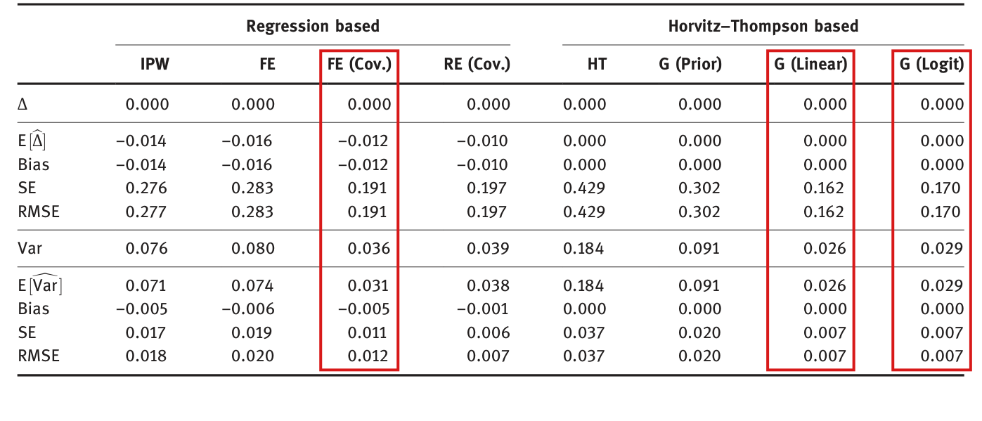
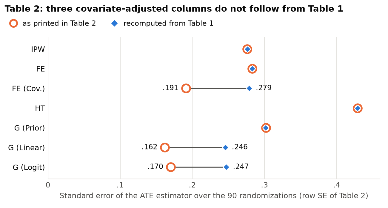
Three columns of Table 2 do not follow from the population printed in Table 1: for that population the standard errors of FE (Cov.), G (Linear) and G (Logit) are .279, .246 and .247, not .191, .162 and .170, and the gain in precision from covariate adjustment is smaller than the table shows.

Table 2, columns FE (Cov.), G (Linear) and G (Logit), p. 149 (PDF p. 15); compare Table 1, column XiX_i, p. 147 (PDF p. 13), and Section 7.1, p. 148 (PDF p. 14)

See also under Formal statements (Lean): P026-T6, P026-T7, P026-T14, P026-T19

As printed

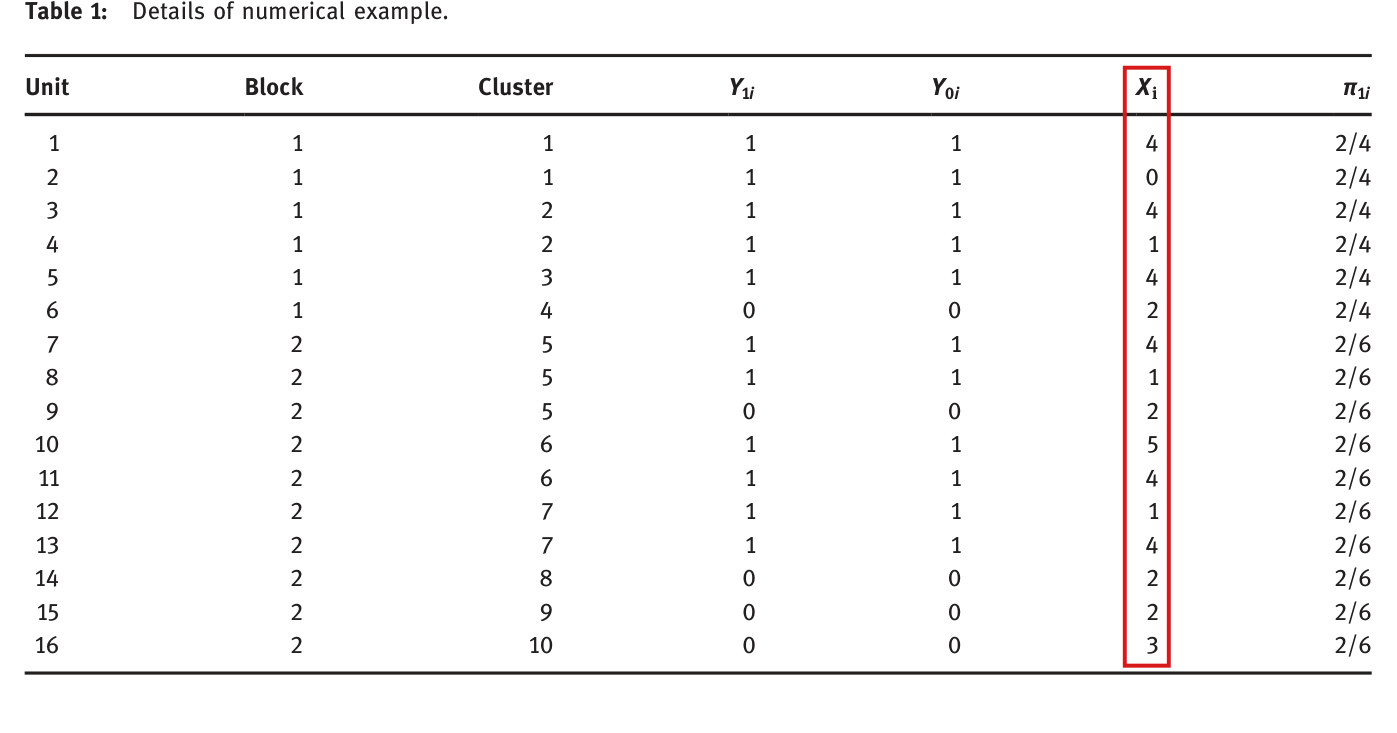
Table 1 gives Xi=(4,0,4,1,4,2,4,1,2,5,4,1,4,2,2,3)X_i=(4,0,4,1,4,2,4,1,2,5,4,1,4,2,2,3) for units 1 to 16.

Table 2, p. 149: three of the eight columns as printed.
FE (Cov.)G (Linear)G (Logit)
Δ\Delta0.0000.0000.000
E[Δ^]\mathrm{E}[\widehat{\Delta}]−0.012\colorbox{#ffe58a}{$-0.012$}0.0000.000
Bias−0.012\colorbox{#ffe58a}{$-0.012$}0.0000.000
SE0.1910.1620.170
RMSE0.1910.1620.170
Var0.0360.0260.029
E[Var⁡^]\mathrm{E}[\widehat{\operatorname{Var}}]0.0310.0260.029
Bias−0.005\colorbox{#ffe58a}{$-0.005$}0.0000.000
SE0.0110.0070.007
RMSE0.0120.0070.007
The problem

Table 2 reports, for the population of Table 1 and the estimators of Section 7.1, the moments of each estimator over the 90 possible randomizations. When they are recomputed from the printed population, three of the four columns that use the covariate XX differ from the table. For G (Linear) the standard error is .246.246 and the variance .060.060, where the table has .162.162 and .026.026. For G (Logit) the standard error is .247.247, and for FE (Cov.) it is .279.279. The variances differ by a factor of about two, which rounding cannot explain. All 40 entries of the four columns that do not use XX (IPW, FE, HT and G (Prior)) agree with the table to the third decimal.

The example overstates the gain from covariate adjustment. Relative to IPW, the standard error of G (Linear) is lower by about 11%, and not by the 41% that the printed .162.162 and .276.276 imply.

I have not established which of the two tables is misprinted. The commands and inputs behind Table 2 are not among the replication files. If XX is changed to 2,3,3,32,3,3,3 for units 2, 4, 8 and 12, where Table 1 has 0,1,1,10,1,1,1, the printed columns are nearly reproduced, but one entry is not (the RMSE of the FE (Cov.) variance estimator is .01255.01255, which rounds to .013.013 against the printed .012.012), and I have found no evidence that these values were used. The RE (Cov.) column is not settled either. The version of lme4 that the paper cites (0.999375-37) could not be run, and version 1.1-37 does not reproduce the column. With REML the estimator has mean −.008-.008 and standard error .303.303, and its variance estimator has bias +.002+.002. With maximum likelihood the variance estimator has negative bias. Whether “all of the regression-based estimators, including variance estimators, are negatively biased” (Section 7.2) holds for the variance estimator of the random-effects fit remains open.

Evidence an exact counterexample

This correction rests on a recalculation over all 90 randomizations. For G (Linear) the recalculation is exact. Least squares on the opposite block gives the predictions 1/4+Xi/81/4+X_i/8 for the units of block 1 and 70/93+Xi/3170/93+X_i/31 for the units of block 2. The estimator has mean 00 and variance 38307/634880≈.06033738307/634880\approx .060337, and the variance estimator [35] has mean 38307/63488038307/634880 and standard error .012370.012370. For G (Logit) both logistic fits have unique finite maximum-likelihood estimates, and the moments are computed to high precision. The mean and standard error of FE (Cov.) do not depend on the variance-estimator convention. I computed its variance-estimator rows using the cluster-robust estimator with the finite-sample factor (10/9)⋅15/(16−K)(10/9)\cdot 15/(16-K), where KK is the number of regressors, the intercept included. The paper does not state this factor. With it, the recalculation reproduces the IPW and FE columns. A second, independent calculation agrees with these values.

Table 2 as printed and as recomputed from the population of Table 1, for the three columns that differ. Each column of the table is followed by its recomputed values.
FE (Cov.)recomputedG (Linear)recomputedG (Logit)recomputed
Δ\Delta.000.000.000.000.000.000
E[Δ^]\mathrm{E}[\widehat{\Delta}]−.012-.012−.014-.014.000.000.000.000
Bias−.012-.012−.014-.014.000.000.000.000
SE.191.279.162.246.170.247
RMSE.191.279.162.246.170.247
Var.036.078.026.060.029.061
E[Var⁡^]\mathrm{E}[\widehat{\operatorname{Var}}].031.072.026.060.029.061
Bias−.005-.005−.006-.006.000.000.000.000
SE.011.019.007.012.007.013
RMSE.012.020.007.012.007.013
What survives

The four columns that do not use XX stand as printed. For the printed population the estimators G (Linear) and G (Logit) remain unbiased, and so do their variance estimators. They still have lower RMSE than IPW, FE and FE (Cov.), by a smaller margin: .246.246 and .247.247 against .277.277, .283.283 and .279.279. They also have lower RMSE than the random-effects fits obtained with version 1.1-37 of lme4. The comparison with the RE (Cov.) column as printed is not settled. No formula, proof or theoretical result uses the entries of Table 2.

Corrected

For the population printed in Table 1, the three columns of Table 2 read as follows.

Table 2, three columns recomputed from Table 1.
FE (Cov.)G (Linear)G (Logit)
Δ\Delta0.0000.0000.000
E[Δ^]\mathrm{E}[\widehat{\Delta}]−0.014\colorbox{#ffe58a}{$-0.014$}0.0000.000
Bias−0.014\colorbox{#ffe58a}{$-0.014$}0.0000.000
SE0.2790.2460.247
RMSE0.2790.2460.247
Var0.0780.0600.061
E[Var⁡^]\mathrm{E}[\widehat{\operatorname{Var}}]0.0720.0600.061
Bias−0.006\colorbox{#ffe58a}{$-0.006$}0.0000.000
SE0.0190.0120.013
RMSE0.0200.0120.013

The FE (Cov.) variance-estimator rows here use the cluster-robust estimator with the factor G(N−1)/((G−1)(N−K))G(N-1)/((G-1)(N-K)), for G=10G=10 clusters, N=16N=16 units and KK regressors, including the intercept, and this convention should be stated. In Section 7.2 the comparison becomes: for this population, G (Linear) and G (Logit) are unbiased and have lower RMSE than IPW, FE and FE (Cov.). The RE (Cov.) column, and the statement that the variance estimators of all regression-based estimators are negatively biased, should be reconciled with the original inputs and settings. If Table 1 and not Table 2 carries the misprint, the correction belongs in the column XiX_i of Table 1, and it requires the original inputs.

Crop of Table 2, which has eight columns of estimator properties: IPW, FE, FE (Cov.), RE (Cov.), HT, G (Prior), G (Linear) and G (Logit), and ten rows. Red boxes mark the whole columns FE (Cov.), G (Linear) and G (Logit), whose SE entries are 0.191, 0.162 and 0.170.
Table 2, p. 149 (PDF p. 15). The three marked columns do not follow from the population of Table 1 and the estimators of Section 7.1; within the two G columns the entries equal to 0.000 stand.
Crop of Table 1, which lists for each of 16 units its block, cluster, two potential outcomes, the covariate X-i and the probability of treatment. A red box marks the column X-i, with the values 4, 0, 4, 1, 4, 2, 4, 1, 2, 5, 4, 1, 4, 2, 2, 3.
Table 1, p. 147 (PDF p. 13). The marked column is the covariate from which the three columns of Table 2 were recomputed.
Dot plot with one row for each of seven estimators and a horizontal axis from 0 to .46 for the standard error of the ATE estimator. For IPW, FE, HT and G (Prior) the open circle for the printed value and the filled diamond for the recomputed value nearly coincide, at about .28, .28, .43 and .30. For FE (Cov.) the printed value is .191 and the recomputed value .279; for G (Linear), .162 and .246; for G (Logit), .170 and .247.
The SE row of Table 2 as printed and as recomputed from Table 1 over the 90 randomizations, for the seven estimators recomputed. The four columns that do not use XX agree with the table; FE (Cov.), G (Linear) and G (Logit) do not. RE (Cov.) is not shown because its recalculation is not settled.

Minor (5)

Real but inconsequential, for example a misprint that does not change a result.

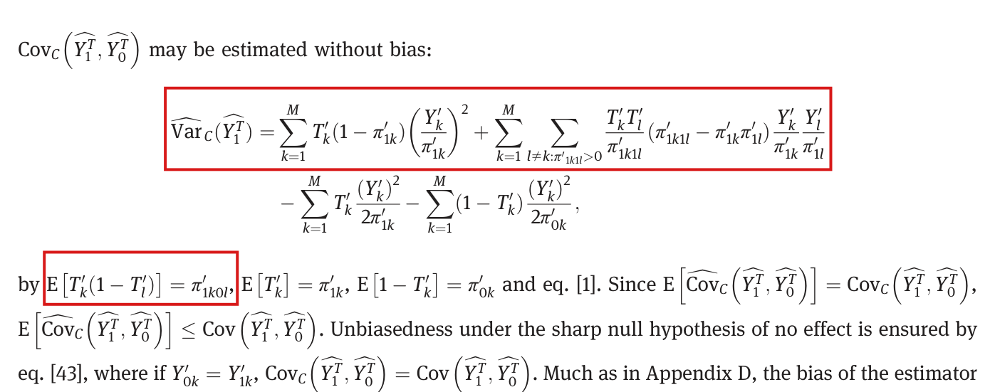
The display in Appendix E that should state the estimator of the covariance bound carries the label and the first two terms of the variance estimator for the treatment total; it should be equation [34].

Appendix E, unnumbered display after “Cov⁡C(Y1T^,Y0T^)\operatorname{Cov}_C(\widehat{Y_1^T},\widehat{Y_0^T}) may be estimated without bias:”, p. 152 (PDF p. 18)

See also under Formal statements (Lean): P026-T8, P026-T9

As printed

“Cov⁡C(Y1T^,Y0T^)\operatorname{Cov}_C\left(\widehat{Y_1^T},\widehat{Y_0^T}\right) may be estimated without bias:”

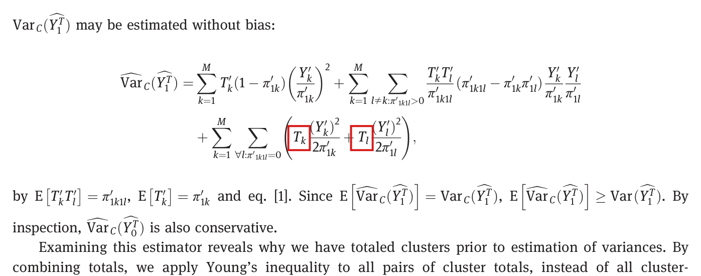
Var⁡^C(Y1T^)=∑k=1MTk′(1−π1k′)(Yk′π1k′)2+∑k=1M∑l≠k:π1k1l′>0Tk′Tl′π1k1l′(π1k1l′−π1k′π1l′)Yk′π1k′Yl′π1l′−∑k=1MTk′(Yk′)22π1k′−∑k=1M(1−Tk′)(Yk′)22π0k′,\begin{aligned} {}\colorbox{#ffe58a}{$\displaystyle \widehat{\operatorname{Var}}_C(\widehat{Y_1^T})$}={}&{}\colorbox{#ffe58a}{$\displaystyle \sum_{k=1}^{M}T'_k(1-\pi'_{1k})\left(\frac{Y'_k}{\pi'_{1k}}\right)^2$}+\colorbox{#ffe58a}{$\displaystyle \sum_{k=1}^{M}\sum_{l\ne k:\pi'_{1k1l}>0}\frac{T'_kT'_l}{\pi'_{1k1l}}(\pi'_{1k1l}-\pi'_{1k}\pi'_{1l})\frac{Y'_k}{\pi'_{1k}}\frac{Y'_l}{\pi'_{1l}}$}\\ &-\sum_{k=1}^{M}T'_k\frac{(Y'_k)^2}{2\pi'_{1k}}-\sum_{k=1}^{M}(1-T'_k)\frac{(Y'_k)^2}{2\pi'_{0k}}, \end{aligned}

“by E[Tk′(1−Tl′)]=π1k0l′\mathrm{E}[T'_k(1-T'_l)]=\pi'_{1k0l}, E[Tk′]=π1k′\mathrm{E}[T'_k]=\pi'_{1k}, E[1−Tk′]=π0k′\mathrm{E}[1-T'_k]=\pi'_{0k} and eq. [1].”

The problem

The sentence before the display and the proof after it concern the covariance bound Cov⁡C\operatorname{Cov}_C of equation [43]. The left side of the display is the label of the variance estimator for the treatment total, and its first row has the two leading terms of that estimator, equation [32]. Only the last two sums belong to the covariance estimator. The expectation of the expression as printed is not Cov⁡C\operatorname{Cov}_C, and the identity E[Tk′(1−Tl′)]=π1k0l′\mathrm{E}[T'_k(1-T'_l)]=\pi'_{1k0l} invoked after the display concerns a factor that the display does not contain. The estimator meant is equation [34] of the main text.

Evidence an exact counterexample

This correction rests on an exact counterexample to the display as printed and on a derivation for the corrected display.

Counterexample. Let N=M=4N=M=4, with each unit its own cluster, and let two of the four units be treated, each of the six subsets having probability 1/61/6. Let Y1k′=Y0k′Y'_{1k}=Y'_{0k} take the values 1,2,4,71,2,4,7. Then π1k′=π0k′=1/2\pi'_{1k}=\pi'_{0k}=1/2, and for k≠lk\ne l the joint probabilities are π1k1l′=π0k0l′=1/6\pi'_{1k1l}=\pi'_{0k0l}=1/6 and π1k0l′=1/3\pi'_{1k0l}=1/3, all positive. If uu and vv are the two treated outcomes, the printed right side equals 2(u−v)2−702(u-v)^2-70, and equation [34] equals the product of the treated and the control outcome sums minus 7070. The printed right side has expectation −42-42. The covariance of the two estimated totals, the bound [43] and the expectation of [34] all equal −28-28.

The six randomizations of the design with four units, each with probability 1/61/6, under the sharp null with outcomes 1,2,4,71,2,4,7.
Treated unitsY1T^\widehat{Y_1^T}Y0T^\widehat{Y_0^T}Display as printedEquation [34]
{1,2}\{1,2\}662222−68-68−37-37
{1,3}\{1,3\}10101818−52-52−25-25
{1,4}\{1,4\}1616121222−22-22
{2,3}\{2,3\}12121616−62-62−22-22
{2,4}\{2,4\}18181010−20-20−25-25
{3,4}\{3,4\}222266−52-52−37-37
Expectation14141414−42-42−28-28

Derivation. Suppose that π1k0l′>0\pi'_{1k0l}>0 for all k≠lk\ne l. Since Tk′(1−Tl′)Yk′Yl′=Tk′(1−Tl′)Y1k′Y0l′T'_k(1-T'_l)Y'_kY'_l=T'_k(1-T'_l)Y'_{1k}Y'_{0l}, the cross term of [34] has expectation (π1k0l′−π1k′π0l′)Y1k′Y0l′/(π1k′π0l′)(\pi'_{1k0l}-\pi'_{1k}\pi'_{0l})Y'_{1k}Y'_{0l}/(\pi'_{1k}\pi'_{0l}). The two remaining sums have expectations ∑k(Y1k′)2/2\sum_k(Y'_{1k})^2/2 and ∑k(Y0k′)2/2\sum_k(Y'_{0k})^2/2. Summing, I obtain E[Cov⁡^C]=Cov⁡C\mathrm{E}[\widehat{\operatorname{Cov}}_C]=\operatorname{Cov}_C, the right side of [43]. Equations [30] and [43] imply that

Cov⁡(Y1T^,Y0T^)−Cov⁡C(Y1T^,Y0T^)=12∑k=1M(Y1k′−Y0k′)2≥0,\operatorname{Cov}\left(\widehat{Y_1^T},\widehat{Y_0^T}\right)-\operatorname{Cov}_C\left(\widehat{Y_1^T},\widehat{Y_0^T}\right)=\frac12\sum_{k=1}^{M}(Y'_{1k}-Y'_{0k})^2\ge 0,

with equality under the sharp null.

What survives

Equation [34] is printed correctly in the main text, and equation [35] is built from it and not from this display, so that the misprint does not reach the variance estimator. The identity [30] and the bound [43] are unaffected. In the example of Section 7 the variance of Δ^HT\widehat{\Delta}_{HT} and the expectation of [35] both equal 353/1920353/1920, which rounds to the 0.1840.184 of Table 2. The corrected display has the stated expectation when π1k0l′>0\pi'_{1k0l}>0 for all k≠lk\ne l. The case in which some π1k0l′\pi'_{1k0l} vanishes is the subject of P026-E002.

Corrected

Suppose that π1k0l′>0\pi'_{1k0l}>0 for all k≠lk\ne l. Then “Cov⁡C(Y1T^,Y0T^)\operatorname{Cov}_C\left(\widehat{Y_1^T},\widehat{Y_0^T}\right) may be estimated without bias:”

Cov⁡^C(Y1T^,Y0T^)=∑k=1M∑l≠kTk′(1−Tl′)π1k0l′(π1k0l′−π1k′π0l′)Yk′Yl′π1k′π0l′−∑k=1MTk′(Yk′)22π1k′−∑k=1M(1−Tk′)(Yk′)22π0k′,\begin{aligned} {}\colorbox{#ffe58a}{$\displaystyle \widehat{\operatorname{Cov}}_C\left(\widehat{Y_1^T},\widehat{Y_0^T}\right)$}={}&{}\colorbox{#ffe58a}{$\displaystyle \sum_{k=1}^{M}\sum_{l\ne k}\frac{T'_k(1-T'_l)}{\pi'_{1k0l}}(\pi'_{1k0l}-\pi'_{1k}\pi'_{0l})\frac{Y'_kY'_l}{\pi'_{1k}\pi'_{0l}}$}\\ &-\sum_{k=1}^{M}T'_k\frac{(Y'_k)^2}{2\pi'_{1k}}-\sum_{k=1}^{M}(1-T'_k)\frac{(Y'_k)^2}{2\pi'_{0k}}, \end{aligned}

“by E[Tk′(1−Tl′)]=π1k0l′\mathrm{E}[T'_k(1-T'_l)]=\pi'_{1k0l}, E[Tk′]=π1k′\mathrm{E}[T'_k]=\pi'_{1k}, E[1−Tk′]=π0k′\mathrm{E}[1-T'_k]=\pi'_{0k} and eq. [1].” This is equation [34]. The rest of the proof stands: E[Cov⁡^C(Y1T^,Y0T^)]=Cov⁡C(Y1T^,Y0T^)≤Cov⁡(Y1T^,Y0T^)\mathrm{E}[\widehat{\operatorname{Cov}}_C(\widehat{Y_1^T},\widehat{Y_0^T})]=\operatorname{Cov}_C(\widehat{Y_1^T},\widehat{Y_0^T})\le\operatorname{Cov}(\widehat{Y_1^T},\widehat{Y_0^T}), with equality when Y0k′=Y1k′Y'_{0k}=Y'_{1k} for all kk.

Crop of the sentence 'Cov-C of the two estimated totals may be estimated without bias', the two-row display that follows it, and three lines of the proof. One red box encloses the first row of the display, whose left side reads 'Var-hat-C of Y-hat-1-T' and whose two terms contain T-prime-k and the product T-prime-k T-prime-l with pi-prime-1k1l. A second red box marks the identity 'E of T-prime-k times one minus T-prime-l equals pi-prime-1k0l' at the start of the proof.
Appendix E, p. 152 (PDF p. 18). The first row of the display, marked, has the label and the two leading terms of the variance estimator [32]; the identity marked below it, on which the proof relies, concerns the factor Tk′(1−Tl′)T'_k(1-T'_l), which the display does not contain.

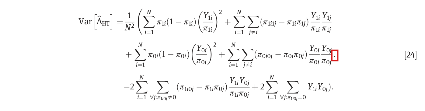
Four misprints: πi\pi_i should read π1i\pi_{1i} in the cluster-total display, “Imai [40]” should read “Imai [39]” in footnote 8, TkT_k and TlT_l should read Tk′T'_k and Tl′T'_l in the last row of the Appendix D display, and the full stop inside equation [24] should be deleted.

Section 6.3, display that rewrites Y1,HTT^\widehat{Y^T_{1,HT}}, p. 144 (PDF p. 10); footnote 8, p. 145 (PDF p. 11); Appendix D, last row of the estimator display, p. 152 (PDF p. 18); equation [24], second row, p. 143 (PDF p. 9)

See also under Formal statements (Lean): P026-T10, P026-T11, P026-T12

As printed

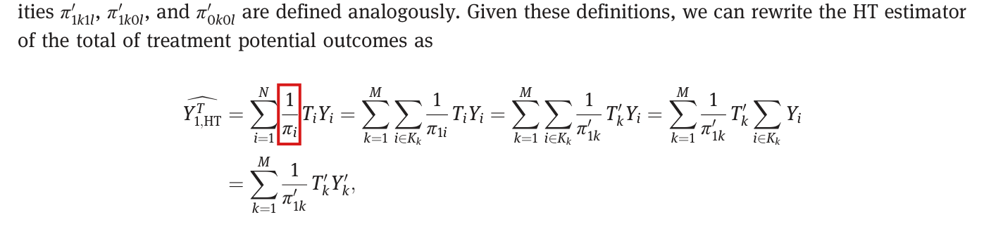
(a) p. 144:

Y1,HTT^=∑i=1N1πiTiYi=∑k=1M∑i∈Kk1π1iTiYi=∑k=1M∑i∈Kk1π1k′Tk′Yi=∑k=1M1π1k′Tk′∑i∈KkYi=∑k=1M1π1k′Tk′Yk′,\widehat{Y^T_{1,HT}}=\sum_{i=1}^{N}\frac{1}{\colorbox{#ffe58a}{$\displaystyle \pi_i$}}T_iY_i=\sum_{k=1}^{M}\sum_{i\in K_k}\frac{1}{\pi_{1i}}T_iY_i=\sum_{k=1}^{M}\sum_{i\in K_k}\frac{1}{\pi'_{1k}}T'_kY_i=\sum_{k=1}^{M}\frac{1}{\pi'_{1k}}T'_k\sum_{i\in K_k}Y_i=\sum_{k=1}^{M}\frac{1}{\pi'_{1k}}T'_kY'_k,

(b) p. 145, footnote 8: “The variance estimators derived in this paper do not reduce to those proposed by Neyman [49], Imai [40] or Middleton and Aronow [5], due to differences in how the covariance term is approximated.”

(c) p. 152, Appendix D, last row of the display for Var⁡^C(Y1T^)\widehat{\operatorname{Var}}_C(\widehat{Y_1^T}):

+∑k=1M∑∀l:π1k1l′=0(Tk(Yk′)22π1k′+Tl(Yl′)22π1l′),+\sum_{k=1}^{M}\sum_{\forall l:\pi'_{1k1l}=0}\left(\colorbox{#ffe58a}{$\displaystyle T_k$}\frac{(Y'_k)^2}{2\pi'_{1k}}+\colorbox{#ffe58a}{$\displaystyle T_l$}\frac{(Y'_l)^2}{2\pi'_{1l}}\right),

(d) p. 143, second row of equation [24]:

+∑i=1Nπ0i(1−π0i)(Y0iπ0i)2+∑i=1N∑j≠i(π0i0j−π0iπ0j)Y0iY0jπ0iπ0j.+\sum_{i=1}^{N}\pi_{0i}(1-\pi_{0i})\left(\frac{Y_{0i}}{\pi_{0i}}\right)^2+\sum_{i=1}^{N}\sum_{j\ne i}(\pi_{0i0j}-\pi_{0i}\pi_{0j})\frac{Y_{0i}Y_{0j}}{\pi_{0i}\pi_{0j}}\colorbox{#ffe58a}{$\displaystyle .$}

The third row continues the expression inside the same parenthesis.

The problem

(a) The paper defines π1i\pi_{1i} and π0i\pi_{0i} and no πi\pi_i, and the next expression in the chain and equation [6] have π1i\pi_{1i}. (b) Reference 40 is Hansen and Bowers. Imai’s paper on variance identification is reference 39, and p. 137 cites it correctly. (c) The cluster indicators are Tk′T'_k. The first row of the same display and the corresponding term of equation [32] carry the primes, and the argument that follows uses E[Tk′]=π1k′\mathrm{E}[T'_k]=\pi'_{1k}. (d) The parenthesis opened in the first row of [24] closes at the end of the third row.

Evidence a check of the printed page

This correction rests on a check of the pages against the adjacent formulas, the definitions on pp. 138 and 144, equations [6], [26] and [32], and the reference list on pp. 153–154.

What survives

Everything else is unaffected. The cluster-total identity, the bound of Appendix D and equation [24] are correct after these repairs.

Corrected

(a)

Y1,HTT^=∑i=1N1π1iTiYi=∑k=1M∑i∈Kk1π1iTiYi=⋯=∑k=1M1π1k′Tk′Yk′.\widehat{Y^T_{1,HT}}=\sum_{i=1}^{N}\frac{1}{\colorbox{#ffe58a}{$\displaystyle \pi_{1i}$}}T_iY_i=\sum_{k=1}^{M}\sum_{i\in K_k}\frac{1}{\pi_{1i}}T_iY_i=\cdots=\sum_{k=1}^{M}\frac{1}{\pi'_{1k}}T'_kY'_k.

(b) “… those proposed by Neyman [49], Imai [39] or Middleton and Aronow [5] …”

(c)

+∑k=1M∑∀l:π1k1l′=0(Tk′(Yk′)22π1k′+Tl′(Yl′)22π1l′),+\sum_{k=1}^{M}\sum_{\forall l:\pi'_{1k1l}=0}\left(\colorbox{#ffe58a}{$\displaystyle T'_k$}\frac{(Y'_k)^2}{2\pi'_{1k}}+\colorbox{#ffe58a}{$\displaystyle T'_l$}\frac{(Y'_l)^2}{2\pi'_{1l}}\right),

(d) The second row of [24] ends without a full stop:

+∑i=1Nπ0i(1−π0i)(Y0iπ0i)2+∑i=1N∑j≠i(π0i0j−π0iπ0j)Y0iπ0iY0jπ0j+\sum_{i=1}^{N}\pi_{0i}(1-\pi_{0i})\left(\frac{Y_{0i}}{\pi_{0i}}\right)^2+\sum_{i=1}^{N}\sum_{j\ne i}(\pi_{0i0j}-\pi_{0i}\pi_{0j})\frac{Y_{0i}}{\pi_{0i}}\frac{Y_{0j}}{\pi_{0j}}
Crop of the two-row display that rewrites the Horvitz-Thompson estimator of the treatment total, with the two lines of text above it. A red box marks the fraction 'one over pi-i' in the first sum; the second sum has 'one over pi-1i'.
Section 6.3, p. 144 (PDF p. 10). In the first sum the marked denominator is πi\pi_i, a symbol that the paper does not define; the next sum has π1i\pi_{1i}.
Crop of footnote 8 with the last line of footnote 7 above it. A red box marks the reference number '[40]' after the name Imai.
Footnote 8, p. 145 (PDF p. 11). The marked reference number should be 39.
Crop of the display for the conservative variance estimator in Appendix D, with the line above it and the four lines of text below it. Red boxes mark the symbols T-k and T-l in the last row, printed without primes; the first row has T-prime-k and T-prime-l.
Appendix D, p. 152 (PDF p. 18). In the last row the two marked indicators lack the prime that the cluster indicators carry in the first row.
Crop of the three rows of equation 24. A red box marks a full stop at the end of the second row, after the fraction Y-0j over pi-0j; the third row continues with minus two times a double sum and ends with the closing parenthesis.
Equation [24], p. 143 (PDF p. 9). The marked full stop ends the second row although the expression continues on the third.

Three words in the text and three entries of the reference list are misprinted: “than” should read “that”, “auxillary” should read “auxiliary”, “In the section” should read “In this section”, Godambe’s article is dated 1955 and its volume number is printed twice, Horvitz and Thompson’s article ends on p. 685, and “post-stratication” should read “post-stratification”.

p. 137 (PDF p. 3), paragraph on Lin [9]; p. 141 (PDF p. 7), last sentence before Section 5.1; p. 142 (PDF p. 8), first sentence of Section 6; references 17, 20 and 37, p. 153 (PDF p. 19)

As printed
  • (a) p. 137: “(and, in fact, the post-stratification-based estimator may be shown to be a special case of the regression-based estimator than Lin proposes).”
  • (b) p. 141: “The simplest way for this assumption to hold is for θi\theta_i to be derived from an auxillary or prior source, but we examine this selection process further in Section 5.1.”
  • (c) p. 142: “In the section, we will provide expressions for the sampling variance of the HT estimator and the generalized difference estimator.”
  • (d) p. 153: “17. Godambe VP. A unified theory of sampling from finite populations. J R Stat Soc Ser B Methodol 17, 1995;17(2):269–278.”
  • (e) p. 153: “20. Horvitz DG, Thompson DJ. A generalization of sampling without replacement from a finite universe. J Am Stat Assoc 1952;47:663–84.”
  • (f) p. 153: “37. Miratrix L, Sekhon J, Yu B. Adjusting treatment effect estimates by post-stratication in randomized experiments. J R Stat Soc Ser B Methodol, 2013;75(2):369–396.”
The problem

These are six misprints. In (d) the year should be 1955, and the volume number 17 appears twice. In (e) the article ends on p. 685. The meaning is clear in each case, and each cited work can still be identified.

Evidence a check of the printed page

This correction rests on a check of the pages and on the publication records of two cited articles. The table of contents of the journal issue lists Godambe’s article as Volume 17, Issue 2, July 1955, pp. 269–278. The JSTOR record of Horvitz and Thompson’s article has Vol. 47, No. 260 (Dec., 1952), pp. 663–685. The paper spells “auxiliary” and “post-stratification” correctly on pp. 142 and 137.

What survives

Everything else is unaffected, since no result depends on these words or entries.

Corrected
  • (a) “… a special case of the regression-based estimator that Lin proposes).”
  • (b) “… derived from an auxiliary or prior source …”
  • (c) “In this section, …”
  • (d) “17. Godambe VP. A unified theory of sampling from finite populations. J R Stat Soc Ser B Methodol 1955;17(2):269–278.”
  • (e) “… J Am Stat Assoc 1952;47:663–85.”
  • (f) “… Adjusting treatment effect estimates by post-stratification in randomized experiments …”
Crop of five lines of the paragraph on Lin and on Miratrix, Sekhon and Yu. A red box marks the word 'than' in 'a special case of the regression-based estimator than Lin proposes'.
Paragraph on Lin, p. 137 (PDF p. 3). The marked word should read “that”.
Crop of the four lines that end Section 5 before the heading of Section 5.1. A red box marks the word 'auxillary' in 'derived from an auxillary or prior source'.
Last sentence before Section 5.1, p. 141 (PDF p. 7). The marked word is misspelled.
Crop of the heading '6 Sampling variance' and the two lines below it. A red box marks the words 'In the section,' at the start of the first line.
First sentence of Section 6, p. 142 (PDF p. 8). The marked words should read “In this section”.
Crop of the reference list from entry 16 to entry 21. Red boxes mark '17, 1995' in the Godambe entry, number 17, and '663-84' in the Horvitz and Thompson entry, number 20.
References 16 to 21, p. 153 (PDF p. 19). In reference 17 the marked volume number is repeated and the marked year should be 1955; in reference 20 the marked page range should end at 685.
Crop of reference entries 36 and 37. A red box marks the word 'post-stratication' in the title of the entry for Miratrix, Sekhon and Yu.
References 36 and 37, p. 153 (PDF p. 19). The marked word in the title is misspelled.

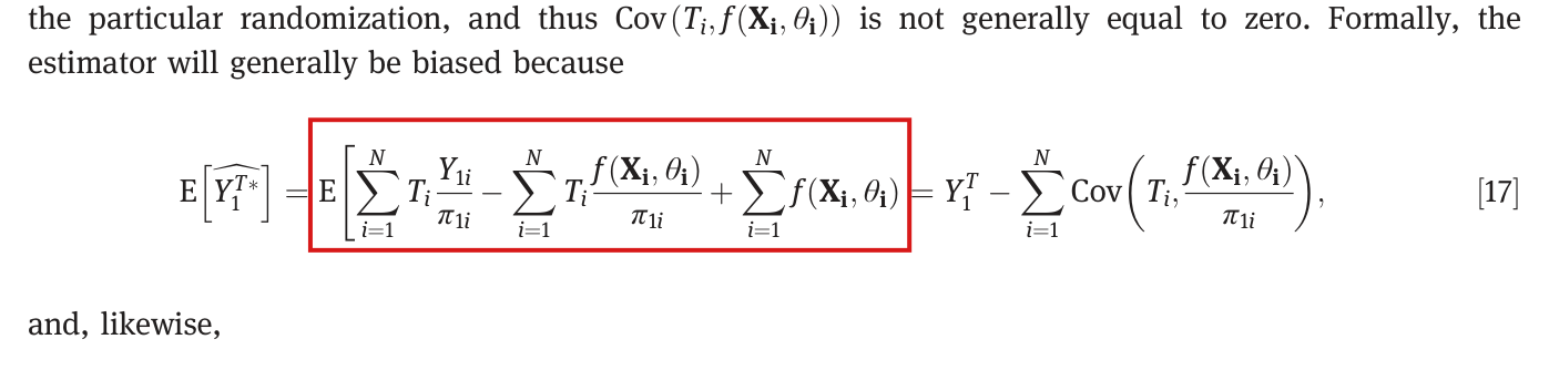
In equation [17] the bracket of the second expectation is not closed; it closes after the third sum.

Section 5.1, equation [17], p. 141 (PDF p. 7)

See also under Formal statements (Lean): P026-T13

As printed
E[Y1T∗^]=E[∑i=1NTiY1iπ1i−∑i=1NTif(Xi,θi)π1i+∑i=1Nf(Xi,θi)=Y1T−∑i=1NCov⁡(Ti,f(Xi,θi)π1i),[17]\mathrm{E}\left[\widehat{Y_1^{T*}}\right]=\mathrm{E}\colorbox{#ffe58a}{$\displaystyle \Bigg[$}\sum_{i=1}^{N}T_i\frac{Y_{1i}}{\pi_{1i}}-\sum_{i=1}^{N}T_i\frac{f(\mathbf{X}_i,\theta_i)}{\pi_{1i}}+\sum_{i=1}^{N}f(\mathbf{X}_i,\theta_i)=Y_1^T-\sum_{i=1}^{N}\operatorname{Cov}\left(T_i,\frac{f(\mathbf{X}_i,\theta_i)}{\pi_{1i}}\right),\qquad\text{[17]}
The problem

The bracket that opens after the second E\mathrm{E} has no closing bracket, and as printed the expectation appears to extend over the equals sign. The identity is correct when the bracket closes after the third sum.

Evidence a derivation

This correction rests on a check of the page and on a short derivation. Since E[Ti]=π1i\mathrm{E}[T_i]=\pi_{1i}, I have

E[Tif(Xi,θi)π1i]=Cov⁡(Ti,f(Xi,θi)π1i)+E[f(Xi,θi)],\mathrm{E}\left[T_i\frac{f(\mathbf{X}_i,\theta_i)}{\pi_{1i}}\right]=\operatorname{Cov}\left(T_i,\frac{f(\mathbf{X}_i,\theta_i)}{\pi_{1i}}\right)+\mathrm{E}\left[f(\mathbf{X}_i,\theta_i)\right],

whether or not f(Xi,θi)f(\mathbf{X}_i,\theta_i) is random. The first sum has expectation Y1TY_1^T, and the terms E[f(Xi,θi)]\mathrm{E}[f(\mathbf{X}_i,\theta_i)] cancel against the expectation of the third sum. Summing over the units, I obtain the right side of [17].

What survives

Everything else is unaffected. The sign and the denominator of the covariance term are correct as printed, and equations [18] and [19] do not change.

Corrected
E[Y1T∗^]=E[∑i=1NTiY1iπ1i−∑i=1NTif(Xi,θi)π1i+∑i=1Nf(Xi,θi)]=Y1T−∑i=1NCov⁡(Ti,f(Xi,θi)π1i).\mathrm{E}\left[\widehat{Y_1^{T*}}\right]=\mathrm{E}\Bigg[\sum_{i=1}^{N}T_i\frac{Y_{1i}}{\pi_{1i}}-\sum_{i=1}^{N}T_i\frac{f(\mathbf{X}_i,\theta_i)}{\pi_{1i}}+\sum_{i=1}^{N}f(\mathbf{X}_i,\theta_i)\colorbox{#ffe58a}{$\displaystyle \Bigg]$}=Y_1^T-\sum_{i=1}^{N}\operatorname{Cov}\left(T_i,\frac{f(\mathbf{X}_i,\theta_i)}{\pi_{1i}}\right).
Crop of equation 17 with the two lines of text above it and the words 'and, likewise,' below it. A red box encloses the expression that begins 'E, open square bracket' and runs through the third sum; no closing bracket appears inside the box or after it.
Equation [17], p. 141 (PDF p. 7). The marked expectation opens a bracket that is not closed before the equals sign.

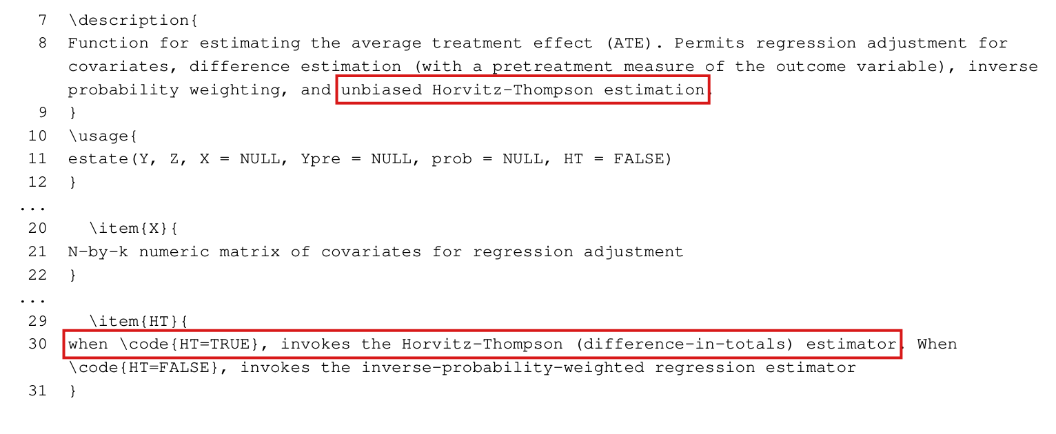
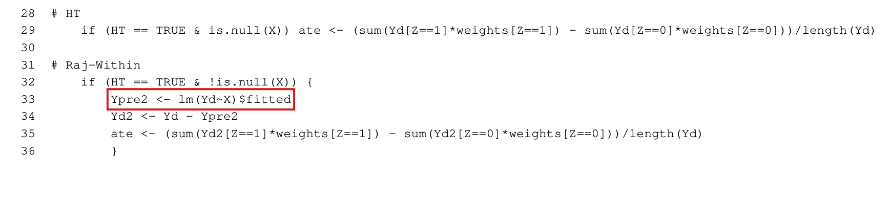
The help page of estate should say that with HT=TRUE and covariates X supplied the function fits a regression using all units, and that the resulting estimator is not unbiased in general.

R package ri (version 0.9), help page of estate (man/estate.Rd, description and argument HT) and R/estate.R, lines 31–36; no passage of the article

See also under Formal statements (Lean): P026-T15

As printed

Help page of estate, description: “Function for estimating the average treatment effect (ATE). Permits regression adjustment for covariates, difference estimation (with a pretreatment measure of the outcome variable), inverse probability weighting, and unbiased Horvitz-Thompson estimation.”

Help page, argument HT: “when HT=TRUE, invokes the Horvitz-Thompson (difference-in-totals) estimator. When HT=FALSE, invokes the inverse-probability-weighted regression estimator”

File R/estate.R, lines 31 to 36: when HT == TRUE and X is supplied, Ypre2 receives the fitted values from regressing Yd on X with lm. The code sets Yd2 to Yd - Ypre2 and computes ate as the weighted difference of the treatment and control residual totals divided by the number of units. The source-code exhibit below shows these lines verbatim.

The problem

With HT=TRUE and X supplied, estate regresses Y (or Y-Ypre when Ypre is supplied) on X, using all units, including unit ii, and applies the Horvitz–Thompson contrast to the residuals. This is the generalized difference estimator with θ\theta fitted from the data at hand. Section 5.1 of the article says that unbiasedness is then not guaranteed, and equation [19] gives the bias. The help page calls Horvitz–Thompson estimation unbiased and describes HT=TRUE as invoking the Horvitz–Thompson estimator, and it does not separate the branch that uses X. A user who combines the two arguments is not told that unbiasedness is no longer guaranteed. The code defines a valid estimator, which adjusts by residuals fitted within the sample. What is missing is the qualification in the help page.

Evidence an exact counterexample

This correction rests on an exact counterexample, computed in rational arithmetic and reproduced by running the package’s code. Suppose that the population has three units, with X=(0,1,2)X=(0,1,2), Y0i=0Y_{0i}=0 and Y1i=1Y_{1i}=1, so that the average treatment effect is 11, and that exactly one unit is treated, each with probability 1/31/3. With prob equal to (1/3,1/3,1/3)(1/3,1/3,1/3), HT=TRUE and X supplied, the function returns 1/41/4, 11 and 1/41/4 for the three randomizations. Its expectation is 1/21/2 and its bias is −1/2-1/2. The covariances of TiT_i with the fitted values are (1/6,0,1/6)(1/6,0,1/6), and by equation [19] the bias is again −(1/3)(3+3/2)(1/6+0+1/6)=−1/2-(1/3)(3+3/2)(1/6+0+1/6)=-1/2. Without X the function returns 11 for every randomization. With Ypre fixed at (0,1,2)(0,1,2) and X=NULL it returns 5/25/2, 11 and −1/2-1/2, with expectation 11.

What survives

No result of the article depends on this branch. Section 7.1 fits its predictions on the opposite block, and its example imposes the sharp null. The article’s results on the Horvitz–Thompson estimator and on the generalized difference estimator under Cov⁡(Ti,f(Xi,θi))=0\operatorname{Cov}(T_i,f(\mathbf{X}_i,\theta_i))=0 are not contradicted, since the bias found is the one that equation [19] predicts. With X=NULL, correct probabilities and a fixed Ypre, the function is unbiased. Predictions that satisfy the covariance condition can be computed outside the function and passed as Ypre. Not every call with X is biased: under the sharp null the fitted values are fixed. The functions gendist and estlate pass X to the same branch.

Corrected

Description: “… inverse probability weighting, and Horvitz-Thompson estimation, which is unbiased when X is NULL, the assignment probabilities are correct, and any Ypre adjustment is fixed before randomization.”

Argument HT: “When HT=TRUE and X=NULL, computes the Horvitz-Thompson difference of totals divided by N, applied to Y (or Y-Ypre). With the correct assignment probabilities and fixed pretreatment Ypre, this is unbiased for the ATE. When HT=TRUE and X is supplied, first fits a least squares regression of Y (or Y-Ypre when Ypre is supplied) on X using all units and applies the same weighted contrast to its residuals. This within-sample covariate adjustment is not generally unbiased for the ATE. To use externally computed adjustments satisfying the covariance condition of the article, pass their prediction vector as Ypre and leave X NULL. When HT=FALSE, invokes the inverse-probability-weighted regression estimator.”

The code does not change.

Listing in monospaced type of parts of the help source for the function estate: the description, the usage line, the item for the argument X and the item for the argument HT, with line numbers. Red boxes mark the words 'unbiased Horvitz-Thompson estimation' in the description and the words 'when HT=TRUE, invokes the Horvitz-Thompson (difference-in-totals) estimator' in the item for HT.
Package ri, file man/estate.Rd, lines 7–12, 20–22 and 29–31, typeset from the source file with line numbers added; a row of dots stands for the lines left out. The marked words call Horvitz–Thompson estimation unbiased and describe HT=TRUE without separating the case in which X is supplied.
Listing in monospaced type of lines 28 to 36 of the function estate, with line numbers: the branch commented 'HT' and the branch commented 'Raj-Within'. A red box marks line 33, 'Ypre2 is assigned the fitted values of lm of Yd on X'.
Package ri, file R/estate.R, lines 28–36, typeset from the source file with line numbers added. With HT == TRUE and X supplied, the marked line regresses Y (or Y-Ypre when Ypre is supplied) on X, using all units.

Clarity notes

Imprecise or ambiguous wording whose intended meaning is correct; not an error.

The intuition on pp. 140–141 passes from correlation to a strict reduction in variance; with predictions fixed across randomizations, the variance falls exactly when 2Cov⁡(H,F)>Var⁡(F)2\operatorname{Cov}(H,F)>\operatorname{Var}(F) for the outcome total HH and the prediction total FF.

Section 5, sentence after equations [13] and [14], pp. 140–141 (PDF pp. 6–7); compare the warning after equation [19], p. 142 (PDF p. 8)

As printed

pp. 140–141: “In inspecting eq. [13], one intuition is that if f(Xi,θi)f(\mathbf{X}_i,\theta_i) predicts the value of Y1iY_{1i}, then across units in the study population f(Xi,θi)f(\mathbf{X}_i,\theta_i) and Y1iY_{1i} will be correlated. By implication then, ∑i=1NTiY1iπ1i\sum_{i=1}^{N}T_i\frac{Y_{1i}}{\pi_{1i}} and ∑i=1NTif(Xi,θi)π1i\sum_{i=1}^{N}T_i\frac{f(\mathbf{X}_i,\theta_i)}{\pi_{1i}} will be correlated across randomizations, thus yielding Y1T∗^\widehat{Y_1^{T*}} such that Var⁡(Y1T∗^)<Var⁡(Y1T^)\colorbox{#ffe58a}{$\operatorname{Var}\left(\widehat{Y_1^{T*}}\right)<\operatorname{Var}\left(\widehat{Y_1^{T}}\right)$}. The same intuition holds for eq. [14], so that both estimators will typically have precision gains.”

p. 142: “The choice of θi\theta_i may be suboptimal and, if chosen poorly, may increase the variance of the estimate, but, so long as the analyst does not use the data at hand in forming a judgment, there will be no consequence for bias.”

Intended meaning

The passage states an intuition and not a theorem: a prediction that tracks the outcome usually lowers the variance. The words “one intuition” and “typically” qualify it, and p. 142 warns that a poorly chosen θi\theta_i may increase the variance. Read in this way the passage is correct. Read literally, the step from “correlated” to a strict inequality leaves out a condition. Let

H=∑i=1NTiY1iπ1i,F=∑i=1NTif(Xi,θi)π1i,H=\sum_{i=1}^{N}T_i\frac{Y_{1i}}{\pi_{1i}},\qquad F=\sum_{i=1}^{N}T_i\frac{f(\mathbf{X}_i,\theta_i)}{\pi_{1i}},

and suppose that the predictions are fixed across randomizations, so that ∑i=1Nf(Xi,θi)\sum_{i=1}^{N}f(\mathbf{X}_i,\theta_i) is a constant. By equation [13], I have Y1T∗^=H−F+∑i=1Nf(Xi,θi)\widehat{Y_1^{T*}}=H-F+\sum_{i=1}^{N}f(\mathbf{X}_i,\theta_i), and therefore

Var⁡(Y1T∗^)−Var⁡(Y1T^)=Var⁡(F)−2Cov⁡(H,F).\operatorname{Var}\left(\widehat{Y_1^{T*}}\right)-\operatorname{Var}\left(\widehat{Y_1^{T}}\right)=\operatorname{Var}(F)-2\operatorname{Cov}(H,F).

The variance falls exactly when 2Cov⁡(H,F)>Var⁡(F)2\operatorname{Cov}(H,F)>\operatorname{Var}(F), and a positive correlation does not ensure this. Suppose that the population has two units, with Y11=1Y_{11}=1 and Y12=2Y_{12}=2, that exactly one of them is treated, each with probability 1/21/2, and that the predictions are fixed at f=3Y1if=3Y_{1i}. Then HH takes the values 22 and 44, FF takes the values 66 and 1212, and the correlation of HH and FF is 11. A direct computation gives Var⁡(H)=1\operatorname{Var}(H)=1, Var⁡(F)=9\operatorname{Var}(F)=9 and Cov⁡(H,F)=3\operatorname{Cov}(H,F)=3, and the adjusted total takes the values 55 and 11, with variance 44. If the predictions are random, the same identity holds with F−∑i=1Nf(Xi,θi)F-\sum_{i=1}^{N}f(\mathbf{X}_i,\theta_i) in place of FF. The definitions of the estimators, the results on unbiasedness and the warning on p. 142 are unaffected, and no reported number depends on this sentence.

Corrected

“… will be correlated across randomizations. Let HH and FF denote these two totals. When the predictions are fixed across randomizations, the adjusted total has smaller variance than the unadjusted total exactly when 2Cov⁡(H,F)>Var⁡(F)\colorbox{#ffe58a}{$2\operatorname{Cov}(H,F)>\operatorname{Var}(F)$}. Correlation alone does not ensure this, and a poor prediction can increase the variance (see p. 142). The same holds for eq. [14], and both estimators will typically have precision gains when the predictions are good.”

Crop of the first four lines of the page. A red box marks the inequality 'Var of Y-hat-1-T-star is less than Var of Y-hat-1-T', which follows the words 'will be correlated across randomizations, thus yielding'.
Top of p. 141 (PDF p. 7), the end of the sentence that begins on p. 140. The marked inequality is stated as a consequence of correlation alone.
Crop of five lines of the paragraph beginning 'Consider two ways that one might derive theta-i'. A red box marks the words 'may increase the variance of the estimate,'.
Section 5.1, paragraph after equation [19], p. 142 (PDF p. 8). The marked words are the paper’s own warning that a poor choice of θi\theta_i can raise the variance.

“The same treatment condition” means each condition: every pair must have positive probability of being jointly treated and positive probability of being jointly in control.

Section 6.4, first paragraph on p. 146 (PDF p. 12), second sentence, before equation [31]

As printed

“First, let us derive an unbiased estimator of Var⁡(Y1T^)\operatorname{Var}(\widehat{Y_1^T}) under the assumption that, for all pairs k,lk,l, π1k1l′\pi'_{1k1l} and π0k0l′>0\pi'_{0k0l}>0. This assumption is equivalent to assuming that all pairs of units have nonzero probability of being assigned to the same treatment condition.”

Intended meaning

The assumption is the one printed in symbols: π1k1l′>0\pi'_{1k1l}>0 and π0k0l′>0\pi'_{0k0l}>0 for all pairs. The second sentence restates it loosely. The example that follows it, of pair-randomized studies in which the two units of a pair are never jointly treated, shows that joint assignment to each condition is meant, and equation [31] is unbiased under that assumption. Read literally, the second sentence says only that Pr⁡(Tk′=Tl′)=π1k1l′+π0k0l′>0\Pr(T'_k=T'_l)=\pi'_{1k1l}+\pi'_{0k0l}>0, which is weaker. With three clusters of one unit each, exactly one of which is treated, each with probability 1/31/3, every pair of distinct clusters has π0k0l′=1/3\pi'_{0k0l}=1/3 and π1k1l′=0\pi'_{1k1l}=0. The pair is then assigned to the same condition with probability 1/31/3, and the assumption fails. That the sentence speaks of pairs of units and not of clusters is not an error. Two units in different clusters have the joint probabilities of their clusters, and two units of one cluster are jointly treated and jointly in control with the positive marginal probabilities of that cluster. No formula or result changes.

Corrected

“This assumption is equivalent to assuming that every pair of units has positive probability of being jointly assigned to treatment and positive probability of being jointly assigned to control.”

Crop of the five lines that precede equation 31. A red box marks the words 'the same treatment condition.' at the end of the sentence 'This assumption is equivalent to assuming that all pairs of units have nonzero probability of being assigned to the same treatment condition'.
Section 6.4, first paragraph on p. 146 (PDF p. 12). The marked words paraphrase the assumption stated in symbols in the sentence before.

Formal statements (Lean)

Formal results: 21 whole; 0 restricted; 3 refuted; 0 omitted.

Coverage concerns the identified claim under its stated assumptions. A checked proof establishes the formal statement; correspondence to the published text was reviewed by AI. Repository access is currently required to open the source links.

Each result links to its current formal statement and proof. “Whole” covers the identified claim under its assumptions; “restricted” covers the stated narrower scope; “refuted” gives a counterexample to the identified assertion; “omitted” has no current theorem. Any named published theorem used as a premise remains an assumption. Browse the formal results for this work.

Section 6.3, sentence before eq. [30] ('Since, for all pairs k,l such that k != l, Pr(T'_k != T'_l) > 0, then pi'_{1k0l} > 0 for all l != k'), and the claims that rest on it: eq. [34] is nonpositively biased, eq. [35] is conservative, and eq. [35] is exactly unbiased under the sharp null; as printed

p. 145 (PDF p. 11); p. 146 (PDF p. 12); p. 147 (PDF p. 13)

pp. 145-147 (PDF pp. 11-13). The printed claim is false: the uniform sharp-null designs on 00,01,11 and on the fourteen six-bit allocations with three treated and T1 ≤ T2 satisfy positive marginals, positive same-arm joints and distinct cluster indicators, but have Pr(T1=1,T2=0)=0. Literal equation [34] contains 0/0 and is outside its domain. For the two-cluster design the marginals are (1/3,2/3) and (2/3,1/3), both same-arm joints and disagreement are 1/3, HT=(-9/4,0,9/4), and [35]= (57/16,3/2,57/16). Its true variance is 27/8, the expected [35] is 23/8 and the bias is -1/2; [34] with the unavailable term omitted is always -9/4, exceeding the true covariance -13/4 by 1. For the six-cluster design the treatment marginals are (2/7,5/7,1/2,1/2,1/2,1/2), the same-arm minimum is 1/14 and the disagreement minimum is 3/7 at {1,2}. The 00,01,11 groups have sizes 4,6,4, HT values -3/20,0,3/20 and [35] values -619/3600,7/54,-619/3600. The true variance is 9/700, the expected [35] is -269/6300 and the bias is -1/18; the covariance is 27/175 and the zero-omitted [34] has expectation 202/175. Both covariance biases are +1. These facts refute the support deduction, conservativeness and the stated sharp-null equalities. Usual measure-theoretic conditions are assumed and hold automatically for these finite laws.

Historical component credits
  • Counterexample proved AronowAudit.P026.asymmetricTwo_counterexample Historical support retained; baseline fidelity: ok; manifest: used; used in Solution; The empty realized arms on 00 and 11 are allowed by the printed positive-marginal assumptions; the six-cluster witness additionally handles fixed nonempty arms. The undefined covariance ratio is not silently treated as the literal printed statistic. No claim-stage verdict changed after reading the record.
  • Counterexample proved AronowAudit.P026.asymmetricSix_counterexample Historical support retained; baseline fidelity: ok; manifest: used; used in Solution; This is a witness refuting the printed support and eq. [35] claims, not an assertion that literal eq. [34] has a defined value. The exact marginal/minimum and grouped per-allocation details in the target are supplementary to the component credited to this row. No claim-stage verdict changed after reading the record.

Section 6.3 (sentence before eq. [30]) and Section 6.4 (eqs. [34], [35], the sentences after them, footnote 9), corrected by adding the missing bound for cluster pairs with pi'_{1k0l} = 0; no design assumption is added

p. 145 (PDF p. 11); pp. 146-147 (PDF pp. 12-13); Appendix E, p. 152 (PDF p. 18)

p. 145 (PDF p. 11); pp. 146-147 (PDF pp. 12-13); Appendix E, p. 152 (PDF p. 18). Adding the unavailable directed-pair bounds gives the exact covariance and variance biases, conservativeness, sharp-null equality characterization, and fixed-prediction residual versions, with the strict six-cluster witness.

Historical component credits
  • Proved AronowAudit.P026.PaperScope.disagreement_identity_T2 Historical support retained; baseline fidelity: ok; manifest: used; used in Solution; Distinctness and pairwise separation are in the standing cluster definition even though the underlying algebraic identity is valid without them. No claim-stage verdict changed after reading the record.
  • Proved AronowAudit.P026.PaperScope.disagreement_positive_iff_T2 Historical support retained; baseline fidelity: ok; manifest: used; used in Solution; Although the standing separation premise makes the left side positive, the right side is not a structure field or an assumed joint-positivity conclusion; it follows from the binary allocation law. No claim-stage verdict changed after reading the record.
  • Proved AronowAudit.P026.PaperScope.ht_cluster_covariance_T2 Historical support retained; baseline fidelity: ok; manifest: used; used in Solution; Zero directed joints remain allowed: the denominators are marginal probabilities, which are positive by the stated setting. No claim-stage verdict changed after reading the record.
  • Proved AronowAudit.P026.PaperScope.printed_variance_bias_T2 Historical support retained; baseline fidelity: ok; manifest: used; used in Solution; No positivity of an individual directed or same-arm joint is assumed; cluster separation is supplied by S7. The negative zero-cross-pair product term is retained. No claim-stage verdict changed after reading the record.
  • Proved AronowAudit.P026.PaperScope.corrected_covariance_bias_T2 Historical support retained; baseline fidelity: ok; manifest: used; used in Solution; The estimator is observable from the realized outcomes and fixed design probabilities; no bias conclusion is assumed in a structure or premise. No claim-stage verdict changed after reading the record.
  • Proved AronowAudit.P026.PaperScope.corrected_variance_bias_T2 Historical support retained; baseline fidelity: ok; manifest: used; used in Solution; The meaning of conservative is nonnegative expected bias, exactly S8; pointwise nonnegativity and standard-error unbiasedness are not claimed. No claim-stage verdict changed after reading the record.
  • Proved AronowAudit.P026.PaperScope.corrected_sharp_null_T2 Historical support retained; baseline fidelity: ok; manifest: used; used in Solution; For equal cluster totals arising from different unit outcome vectors, choose the first unit vector as c and rewrite the second cluster-total vector using equality; every statistic in the conclusion is unchanged. No unit-level restriction on the possible common totals results. No claim-stage verdict changed after reading the record.
  • Counterexample proved AronowAudit.P026.repaired_sharp_null_strict_bias Historical support retained; baseline fidelity: ok; manifest: used; used in Solution; The counterexample_proved status identifies a necessity witness for T2(f), not a counterexample to the corrected target itself; target kind and row role are compatible. No claim-stage verdict changed after reading the record.
  • Proved AronowAudit.P026.PaperScope.corrected_variance_decomposition_T2 Historical support retained; baseline fidelity: ok; manifest: used; used in Solution; The positive-weight restriction is explicit in T2(e), so ignoring zero-probability allocations loses no claimed conclusion. No claim-stage verdict changed after reading the record.
  • Proved AronowAudit.P026.PaperScope.corrected_residual_variance_T2 Historical support retained; baseline fidelity: ok; manifest: used; used in Solution; Fixed predictions are an explicit hypothesis of T2(g) and S6, so constancy across allocations is faithful here. Other residual identities follow by specializing the arbitrary outcome vectors in the other T2 rows. No claim-stage verdict changed after reading the record.
  • Proved AronowAudit.P026.PaperScope.correctedBiasExpression_nonneg_T2 Historical support retained; baseline fidelity: ok; manifest: used; used in Solution; This row is the auxiliary square-sum nonnegativity component, not by itself a proof of the variance bias identity; R165-07 supplies that identity. Cluster separation is S7, not an extra support hypothesis. No claim-stage verdict changed after reading the record.
  • Proved AronowAudit.P026.joint_nonneg Historical support retained; baseline fidelity: ok; manifest: used; used in Solution; Auxiliary or certificate fact already contained in the main declarations used for this target; no separate helper statement is included.
  • Proved AronowAudit.P026.joint_diagonal Historical support retained; baseline fidelity: ok; manifest: used; used in Solution; Auxiliary or certificate fact already contained in the main declarations used for this target; no separate helper statement is included.
  • Proved AronowAudit.P026.cross_diagonal Historical support retained; baseline fidelity: ok; manifest: used; used in Solution; Auxiliary or certificate fact already contained in the main declarations used for this target; no separate helper statement is included.
  • Proved AronowAudit.P026.zeroSum_squares_nonneg Historical support retained; baseline fidelity: ok; manifest: used; used in Solution; Auxiliary or certificate fact already contained in the main declarations used for this target; no separate helper statement is included.

Section 6.4, eq. [35] with the sentences after it and footnote 9, and the scope claim 'conservative for any experimental design' (p. 137), corrected by adding the missing hypothesis pi'_{1k0l} > 0 for all pairs of distinct clusters; eqs. [34] and [35] are kept as printed

p. 147 (PDF p. 13); p. 137 (PDF p. 3); eq. [34], p. 146 (PDF p. 12)

p. 147 (PDF p. 13); p. 137 (PDF p. 3); eq. [34], p. 146 (PDF p. 12). Directed cross-arm support is not implied by the standing assumptions, and under that support the printed estimators have the stated biases, conservativeness and sharp-null equalities, also for fixed residuals, with the numerical design's stated attained support minima.

Historical component credits
  • Proved AronowAudit.P026.PaperScope.support_repair_T3 Historical support retained; baseline fidelity: ok; manifest: used; used in Solution; H+ is expressly part of corrected target T3, so it is not an undisclosed restriction. The theorem also gives a valid extension beyond the unit-level sharp-null equality cases. No claim-stage verdict changed after reading the record.
  • Proved AronowAudit.P026.PaperScope.support_residual_variance_T3 Historical support retained; baseline fidelity: ok; manifest: used; used in Solution; Fixed predictions and H+ are both in T3(d); the weaker cluster-total equality antecedent makes the equality conclusion more general without changing the claimed cases. No claim-stage verdict changed after reading the record.
  • Proved AronowAudit.P026.table_support Historical support retained; baseline fidelity: ok; manifest: used; used in Solution; Three separately quantified attaining pairs, together with the universal lower bounds, certify the three actual minima; no claim about fitted estimates is being credited to this support lemma. No claim-stage verdict changed after reading the record.

Section 5.1, second option for deriving theta_i ('If theta_i is a function of any or all of the elements of the set {Y_j : T_i indep T_j} and no other random variables, then T_i indep theta_i ... and therefore Cov(T_i, f(X_i, theta_i)) = 0'), with footnote 5; as printed

p. 142 (PDF p. 8)

p. 142 (PDF p. 8). The printed claim is false: pairwise assignment independence does not pass through an arbitrary nonlinear fit of several outcomes. In the six-unit complementary-XOR design, independence holds exactly between different complementary pairs; the full fitting sets are {3,4,5,6}, {1,2,5,6}, {1,2,3,4} for the three pairs. Each stated fit uses two outcomes in its permitted set and equals its own treatment indicator. The joint event that treatment and the fit are both one has probability 1/2, while the product of their probabilities is 1/4, and their covariance is 1/4. The generalized totals are both 3, the generalized ATE is always zero, and HT=Delta=1. Its bias -1 agrees with [19]. In the three-unit XOR design all distinct coordinates are independent with marginals 1/2; fitting the XOR of the other outcomes again gives generalized ATE zero and bias -1. The alternative product fit has covariance -1/8, expectation 7/6 and bias +1/6. All potential outcomes and covariates are fixed as specified in the witness definitions. Usual measure-theoretic conditions are assumed and automatic on these finite laws.

Historical component credits
  • Counterexample proved AronowAudit.P026.xorSix_counterexample Historical support retained; baseline fidelity: ok; manifest: used; used in Solution; This is an explicit witness refuting the printed assertion, not a proof of the positive assertion or an attempted negation of a different reading. Rational equalities and strict discrepancies embed in ℝ. No claim-stage verdict changed after reading the record.
  • Counterexample proved AronowAudit.P026.xorThree_counterexamples Historical support retained; baseline fidelity: ok; manifest: used; used in Solution; This is an explicit witness refuting the printed assertion, not a proof of the positive assertion or an attempted negation of a different reading. Rational equalities and strict discrepancies embed in ℝ. No claim-stage verdict changed after reading the record.

Section 5.1, second option for deriving theta_i, and footnote 5, corrected: independence of T_i from the whole vector of assignments used in the fit

p. 142 (PDF p. 8)

p. 142 (PDF p. 8). Under the usual measure-theoretic conditions, independence of each focal treatment from the whole assignment vector used by its fit, or more weakly from the whole observed-outcome vector, passes through deterministic fitting and prediction and gives zero covariance. If either premise holds for each unit, allowing a different choice for each unit, both generalized totals and the ATE are unbiased. The fitting prediction factors explicitly through the fitting assignment vector; the scalar footnote follows for one outcome. A three-unit nonlinear fitting witness shows that the scalar argument cannot replace vector independence in general. Pairwise independence suffices for additive predictions with fixed coefficients, with the stated covariance expansion. Mutually independent units justify leave-one-out fits, and independent block vectors justify fitting on other blocks. The nonempty unit type is the guard for the ATE denominator; finite assignment spaces make all measurability and moment conditions automatic. Parameter fitting and fixed covariates can be absorbed in the arbitrary deterministic real-valued map G in the unbiasedness clause.

Historical component credits
  • Proved AronowAudit.P026.unit_vector_fitting_unbiased Limited support; baseline fidelity: narrower; manifest: not used; not used in Solution; Duplicate assignment-vector-only unbiasedness theorem; it does not supply the omitted observed-outcome branch.
  • Proved AronowAudit.P026.independent_comp Historical support retained; baseline fidelity: ok; manifest: used; used in Solution; Auxiliary or certificate fact already contained in the main declarations used for this target; no separate helper statement is included.
  • Proved AronowAudit.P026.PaperScope.vector_fitting_independence_T5 Historical support retained; baseline fidelity: ok; manifest: used; used in Solution; No additional hypotheses beyond the standing model and the identified target component; no claim-stage verdict changed.
  • Proved AronowAudit.P026.PaperScope.outcome_vector_fitting_independence_T5 Historical support retained; baseline fidelity: ok; manifest: used; used in Solution; No additional hypotheses beyond the standing model and the identified target component; no claim-stage verdict changed.
  • Proved AronowAudit.P026.PaperScope.vector_fitting_unbiased_T5 Limited support; baseline fidelity: narrower; manifest: used; used in Solution; {'source': 'adjudication+second review', 'adjudicator': 'P026_PaperScope.lean:235 requires every focal treatment indicator to be independent of fittingAssignments, whereas T5(a) expressly also permits independence of the observed-outcome fitting vector and T5(b) invokes the premise of (a). That weaker-premise unbiasedness conclusion is missing. For example, take independent fair bits A,B, assignments (A,B,A), treatment outcomes (1,1,2), control outcomes (0,0,2), J_0={1,2}, empty other fitting sets, and prediction f_0=Y_1*Y_2=2B with other predictions zero: the observed fitting vector (B,2) is independent of A, while the fitting assignment vector (B,A) is not. This excludes a nonconstant prediction under valid positive marginals; the separate outcome-vector independence lemma at P026_PaperScope.lean:221 does not put the weaker-premise unbiasedness conclusion into this declaration.', 'suggested_fix': 'Replace h by ∀ i, independent E.design (fun w => E.design.treatment w i) (fittingOutcomes E.design (J i) x z), retaining all three unbiasedness conclusions; assignment-vector independence implies this weaker hypothesis.', 'second_review': "The hypothesis of P026_PaperScope.lean:235 requires independence from fittingAssignments, the treatment vector defined at P026_FiniteDesign.lean:782, while T5(a) explicitly also permits independence from the observed-outcome vector and T5(b) invokes that premise for every unit. For independent fair bits A,B, take assignments (A,B,A), treatment outcomes (1,1,2), control outcomes (0,0,2), J_0={1,2}, prediction f_0=Y_1*Y_2=2B, and empty other fitting sets with zero predictions: the observed fitting vector (B,2) is independent of A, but the assignment vector (B,A) is not, despite all marginals being positive. Thus a nontrivial branch of the target's unbiasedness conclusion is excluded; replace the assignment-vector hypothesis by outcome-vector independence while retaining the three conclusions.", 'severity': 'major'}
  • Proved AronowAudit.P026.PaperScope.additive_fitting_unbiased_T5 Historical support retained; baseline fidelity: ok; manifest: used; used in Solution; No additional hypotheses beyond the standing model and the identified target component; no claim-stage verdict changed.
  • Proved AronowAudit.P026.PaperScope.mutually_independent_leave_out_T5 Historical support retained; baseline fidelity: ok; manifest: used; used in Solution; No additional hypotheses beyond the standing model and the identified target component; no claim-stage verdict changed.
  • Proved AronowAudit.P026.PaperScope.mutually_independent_other_blocks_T5 Historical support retained; baseline fidelity: ok; manifest: used; used in Solution; No additional hypotheses beyond the standing model and the identified target component; no claim-stage verdict changed.
  • Proved AronowAudit.P026.covariance_div_right Historical support retained; baseline fidelity: ok; manifest: used; used in Solution; Auxiliary or certificate fact already contained in the main declarations used for this target; no separate helper statement is included.
  • Proved AronowAudit.P026.covariance_const_right Historical support retained; baseline fidelity: ok; manifest: used; used in Solution; Auxiliary or certificate fact already contained in the main declarations used for this target; no separate helper statement is included.
  • Proved AronowAudit.P026.independent_covariance_zero Historical support retained; baseline fidelity: ok; manifest: not used; not used in Solution; Auxiliary or certificate fact already contained in the main declarations used for this target; no separate helper statement is included.
  • Proved AronowAudit.P026.covariance_add_right Historical support retained; baseline fidelity: ok; manifest: used; used in Solution; Auxiliary or certificate fact already contained in the main declarations used for this target; no separate helper statement is included.
  • Proved AronowAudit.P026.covariance_sum_right Historical support retained; baseline fidelity: ok; manifest: used; used in Solution; Auxiliary or certificate fact already contained in the main declarations used for this target; no separate helper statement is included.

Table 2, column G (Linear) (rows SE, RMSE, Var, E[Var-hat], SE, RMSE) and column FE (Cov.) (rows E[Delta-hat], Bias, SE, RMSE, Var), as printed, set against the population of Table 1 and the estimators of Section 7.1

Table 2, p. 149 (PDF p. 15); Table 1, p. 147 (PDF p. 13); Section 7.1, p. 148 (PDF p. 14)

Table 2, p. 149 (PDF p. 15); Table 1, p. 147 (PDF p. 13); Section 7.1, p. 148 (PDF p. 14). The printed claim is false: for the printed sixteen-unit population and its ninety uniform allocations, the unique real OLS fits within blocks 2 and 1 are respectively 1/4+X/8 and 70/93+X/31. Opposite-block predictions have residual cluster totals (1,7/8,1/4,-1/2,-15/31,19/93,1/3,-76/93,-76/93,-79/93). The actual generalized estimator G has mean and bias zero, variance and expected residual variance estimate 38307/634880 (approximately .0603374), and SE=RMSE approximately .2456367. The residual variance estimate is unbiased and has variance 2400328658503/15687787688755200 and SE=RMSE approximately .0123696. The strict rounding refutations for .026, .162 and .007 follow. For every allocation the OLS regression on (1,T,block2,X) has a unique real minimizer; its treatment coefficient is the specified residualized FE formula and both projection denominators are positive. Its mean is approximately -.0139874, its variance .0777347, and its SE .2788094, with the stated broad intervals and rounding refutations of -.012, .036 and .191. Every approximation has error less than .00000005. Usual measure-theoretic conditions are assumed and automatic for this finite law.

Historical component credits
  • Proved AronowAudit.P026.table_treatment_mean_certificate Historical support retained; baseline fidelity: ok; manifest: used; used in Solution; Auxiliary or certificate fact already contained in the main declarations used for this target; no separate helper statement is included.
  • Proved AronowAudit.P026.fe_x_norm Historical support retained; baseline fidelity: ok; manifest: used; used in Solution; Auxiliary nonzero-denominator certificate, not a claim about all covariate populations. No claim-stage verdict change after reading the record.
  • Proved AronowAudit.P026.fe_tx_certificate Historical support retained; baseline fidelity: ok; manifest: used; used in Solution; Auxiliary or certificate fact already contained in the main declarations used for this target; no separate helper statement is included.
  • Proved AronowAudit.P026.table_linear_ht_certificate Historical support retained; baseline fidelity: ok; manifest: used; used in Solution; Auxiliary or certificate fact already contained in the main declarations used for this target; no separate helper statement is included.
  • Proved AronowAudit.P026.table_linear_v_certificate Historical support retained; baseline fidelity: ok; manifest: used; used in Solution; Auxiliary or certificate fact already contained in the main declarations used for this target; no separate helper statement is included.
  • Proved AronowAudit.P026.fe_estimate_certificate Historical support retained; baseline fidelity: ok; manifest: used; used in Solution; Auxiliary or certificate fact already contained in the main declarations used for this target; no separate helper statement is included.
  • Proved AronowAudit.P026.fe_x_certificate Historical support retained; baseline fidelity: ok; manifest: used; used in Solution; Auxiliary or certificate fact already contained in the main declarations used for this target; no separate helper statement is included.
  • Proved AronowAudit.P026.table_linear_fits Historical support retained; baseline fidelity: ok; manifest: used; used in Solution; The numeric moment literals correspond to actual block counts, sums of X and sums of X squared: (6,15,53) and (10,28,96). Full rank also follows directly from distinct covariates in each fixed block; no family of singular fits is excluded. No claim-stage verdict change after reading the record.
  • Proved AronowAudit.P026.table_linear_moments Historical support retained; baseline fidelity: ok; manifest: used; used in Solution; The row establishes the exact moments in T6(A), rather than asserting that the erroneous printed entries are true. No claim-stage verdict change after reading the record.
  • Counterexample proved AronowAudit.P026.table_linear_refutation Historical support retained; baseline fidelity: ok; manifest: used; used in Solution; Read as the stated rounding-separation component of the refutation, together with R167-09 for equality of the variance/mean and SD/RMSE pairs; no universal assertion on a different design is substituted. No claim-stage verdict change after reading the record.
  • Proved AronowAudit.P026.fe_normal_equations Historical support retained; baseline fidelity: ok; manifest: used; used in Solution; Auxiliary regression certificate; no MLE or probabilistic conditional premise is assumed. No claim-stage verdict change after reading the record.
  • Counterexample proved AronowAudit.P026.fe_table_moments Historical support retained; baseline fidelity: ok; manifest: used; used in Solution; Exact refutation witness for the FE ATE rows specified by T6. The target prints the whole FE column, but its named and described component excludes the FE variance-estimator convention; that convention is not being credited here. No claim-stage verdict change after reading the record.

Table 2, columns G (Linear) and FE (Cov.), corrected for the population printed in Table 1

Table 2, p. 149 (PDF p. 15); Table 1, p. 147 (PDF p. 13); Section 7.1, p. 148 (PDF p. 14)

Table 2, p. 149 (PDF p. 15); Table 1, p. 147 (PDF p. 13); Section 7.1, p. 148 (PDF p. 14). For the printed population and ninety equiprobable assignments, the opposite-block lines are the unique OLS fits, and FE (Cov.) is the unique OLS regression on (1,T,block2,X). G (Linear) has mean zero, variance and expected equation [35] variance estimate 38307/634880, and variance-estimator variance 2400328658503/15687787688755200. Its complete corrected column is (0,0,0,.246,.246,.060,.060,0,.012,.012). FE (Cov.) has corrected ATE mean and bias -.014, SE and RMSE .279, and variance .078, with the stated strict mean and variance intervals; G (Linear) has the smaller RMSE. All columns without X are unchanged: HT (0,0,0,.429,.429,.184,.184,0,.037,.037), G (Prior) (0,0,0,.302,.302,.091,.091,0,.020,.020), IPW (0,-.014,-.014,.276,.277,.076,.071,-.005,.017,.018), and FE (0,-.016,-.016,.283,.283,.080,.074,-.006,.019,.020). HT and prior are unbiased, with variance equal to expected equation [35] variance estimate 353/1920 and 233/2560, respectively. Their variance-estimator variances are 10147/7372800 and 20083/52428800. IPW is WLS with inverse observed-arm inclusion weights, and FE is OLS on (1,T,block2); both fits are unique. Their clustered variance estimates use the explicit HC1 convention (10/9)*15/(16-k), k=2,3. All inverses and arm denominators exist on every assignment. The usual measure-theoretic conditions are assumed; here every quantity is a moment of a function on a fixed finite probability space.

Historical component credits
  • Proved AronowAudit.P026.table_treatment_mean_certificate Historical support retained; baseline fidelity: ok; manifest: used; used in Solution; Auxiliary or certificate fact already contained in the main declarations used for this target; no separate helper statement is included.
  • Proved AronowAudit.P026.fe_x_norm Historical support retained; baseline fidelity: ok; manifest: used; used in Solution; Auxiliary positivity needed for the nonzero X projection denominator; the sum uses fixed printed covariates.
  • Proved AronowAudit.P026.fe_tx_certificate Historical support retained; baseline fidelity: ok; manifest: used; used in Solution; Auxiliary or certificate fact already contained in the main declarations used for this target; no separate helper statement is included.
  • Proved AronowAudit.P026.table_linear_ht_certificate Historical support retained; baseline fidelity: ok; manifest: used; used in Solution; Auxiliary or certificate fact already contained in the main declarations used for this target; no separate helper statement is included.
  • Proved AronowAudit.P026.table_linear_v_certificate Historical support retained; baseline fidelity: ok; manifest: used; used in Solution; Auxiliary or certificate fact already contained in the main declarations used for this target; no separate helper statement is included.
  • Proved AronowAudit.P026.fe_estimate_certificate Historical support retained; baseline fidelity: ok; manifest: used; used in Solution; Auxiliary or certificate fact already contained in the main declarations used for this target; no separate helper statement is included.
  • Proved AronowAudit.P026.fe_x_certificate Historical support retained; baseline fidelity: ok; manifest: used; used in Solution; Auxiliary or certificate fact already contained in the main declarations used for this target; no separate helper statement is included.
  • Proved AronowAudit.P026.table_linear_fits Historical support retained; baseline fidelity: ok; manifest: used; used in Solution; All normal equations use observed sharp-null Y values, so the opposite-block coefficients are assignment independent. The determinant numerals equal the determinants of the fixed block data matrices.
  • Proved AronowAudit.P026.table_linear_moments Historical support retained; baseline fidelity: ok; manifest: used; used in Solution; Auxiliary or certificate fact already contained in the main declarations used for this target; no separate helper statement is included.
  • Proved AronowAudit.P026.table_linear_corrected_rounding Historical support retained; baseline fidelity: ok; manifest: used; used in Solution; Auxiliary or certificate fact already contained in the main declarations used for this target; no separate helper statement is included.
  • Proved AronowAudit.P026.fe_normal_equations Historical support retained; baseline fidelity: ok; manifest: used; used in Solution; The fixed block dummy/intercept and X columns are independent; the asserted positive treatment residual norm therefore gives full rank. No result is smuggled into a Design field.
  • Counterexample proved AronowAudit.P026.fe_table_moments Historical support retained; baseline fidelity: ok; manifest: used; used in Solution; Auxiliary or certificate fact already contained in the main declarations used for this target; no separate helper statement is included.
  • Proved AronowAudit.P026.table_unchanged_columns Limited support; baseline fidelity: narrower; manifest: used; used in Solution; Its selected HT/prior moments are already supplied by the aggregate correction; its narrower status does not justify unchanged complete columns.
  • Proved AronowAudit.P026.Refutations.table2_correction_T7 Limited support; baseline fidelity: narrower; manifest: used; used in Solution; {'source': 'adjudication+second review', 'adjudicator': "P026_Refutations.lean:78 presents a complete correction of T7(a)-(d), but its final conjunct gives only selected moments and variance rounding for HT and G (Prior). T7(d) says 'The columns that do not use X are unchanged', which also includes the HT and G (Prior) variance-estimator SE/RMSE entries .037 and .020 and the IPW and FE columns. Neither the variance-estimator second moments needed for those HT/G (Prior) entries nor the IPW/FE results occur in the conclusion. The target's exclusion of unspecified FE (Cov.) variance conventions does not exclude these other columns.", 'suggested_fix': 'Extend the final conjunct to certify the remaining unchanged-column entries, including Var(printedVariance HT)=10147/7372800 and Var(printedVariance G(Prior))=20083/52428800 with SD rounding to .037 and .020, and the IPW/FE column results promised by T7(d).', 'second_review': "T7(d) says 'The columns that do not use X are unchanged', but the final conjunct of the purported complete correction at P026_Refutations.lean:78 gives only selected HT/G (Prior) moments and variance rounding (P026_Refutations.lean:93). It omits their variance-estimator SE/RMSE entries .037 and .020 from the [paper, Table 2](https://www.degruyterbrill.com/document/doi/10.1515/jci-2012-0009/html), as well as the IPW and FE columns covered by that clause. These second-moment and regression results are substantive conclusions, so the complete correction needs an extended statement rather than merely a revised description.", 'severity': 'major'}

Appendix E ('proof of conservative covariance estimator'), with the unnumbered estimator display replaced by eq. [34]

Appendix E, p. 152 (PDF p. 18); eq. [34], p. 146 (PDF p. 12)

Appendix E, p. 152 (PDF p. 18); eq. [34], p. 146 (PDF p. 12). The corrected Appendix E display estimates the covariance lower bound under directed support, with the exact gap and equality characterization.

Historical component credits
  • Proved AronowAudit.P026.PaperScope.ht_cluster_covariance_T8 Historical support retained; baseline fidelity: ok; manifest: used; used in Solution; No additional hypotheses beyond the standing model and the identified target component; no claim-stage verdict changed.
  • Proved AronowAudit.P026.PaperScope.covariance_bound_gap_T8 Historical support retained; baseline fidelity: ok; manifest: used; used in Solution; No additional hypotheses beyond the standing model and the identified target component; no claim-stage verdict changed.
  • Proved AronowAudit.P026.PaperScope.appendixE_corrected_T8 Historical support retained; baseline fidelity: ok; manifest: used; used in Solution; No additional hypotheses beyond the standing model and the identified target component; no claim-stage verdict changed.

Appendix E, unnumbered display after 'Cov_C(Y_1^T-hat, Y_0^T-hat) may be estimated without bias:', as printed

Appendix E, p. 152 (PDF p. 18)

Appendix E, p. 152 (PDF p. 18). The printed claim is false: for four singleton clusters with two treated uniformly, and sharp-null outcomes (1,2,4,7), the literal Appendix E display has the six values (-68,-52,2,-62,-20,-52) and expectation -42. Equation [34] has values (-37,-25,-22,-22,-25,-37) and expectation -28, equal to the true covariance and its population bound; the true treatment-total variance and its population bound are both 28. Every marginal is 1/2 and all distinct-cluster joint probabilities are positive (TT=CC=1/6, TC=1/3). Thus the printed display is unbiased for neither of the quantities named in the text and on its left side. Usual measure-theoretic conditions are assumed and hold automatically on this finite probability space.

Historical component credits
  • Counterexample proved AronowAudit.P026.appendixE_counterexample Historical support retained; baseline fidelity: ok; manifest: used; used in Solution; This is an explicit witness refuting the printed assertion, not a proof of the positive assertion or an attempted negation of a different reading. Rational equalities and strict discrepancies embed in ℝ. No claim-stage verdict changed after reading the record.

Section 6.3, unnumbered display rewriting the HT estimator of the treatment total over cluster totals, with pi_{1i} in the first sum (printed pi_i), and the companion display for the control total

p. 144 (PDF p. 10); p. 145 (PDF p. 11)

p. 144 (PDF p. 10); p. 145 (PDF p. 11). Grouping by the fixed cluster partition preserves each displayed HT total identity and the resulting ATE contrast.

Historical component credits
  • Proved AronowAudit.P026.PaperScope.cluster_aggregation_T10 Historical support retained; baseline fidelity: ok; manifest: used; used in Solution; The universal arm/outcome identity gives both totals and their ATE contrast by taking the difference and using the same population denominator. Positive-disagreement uniqueness is unnecessary for grouping. No claim-stage verdict changed.

Section 6.4, eqs. [31]-[33], and Appendix D ('abbreviated proof of conservative variance estimator') with the cluster indicators T'_k, T'_l restored in the last sum of its estimator display (printed T_k, T_l)

p. 146 (PDF p. 12); Appendix D, pp. 151-152 (PDF pp. 17-18)

p. 146 (PDF p. 12); Appendix D, pp. 151-152 (PDF pp. 17-18). The restored cluster-indicator formulas give the exact arm variance and conservative bounds, unbiased estimation of those bounds, and unbiased equation [31] under same-arm support.

Historical component credits
  • Proved AronowAudit.P026.PaperScope.ht_arm_variance_T11 Historical support retained; baseline fidelity: ok; manifest: used; used in Solution; Separation of distinct cluster indicators and surjectivity of membership are exactly the paper cluster convention. No same-arm or directed cross-arm joint positivity is assumed. No claim-stage verdict change after reading the record.
  • Proved AronowAudit.P026.PaperScope.arm_variance_corrected_T11 Historical support retained; baseline fidelity: ok; manifest: used; used in Solution; The separated-clusters premise comes from standing assumption S7, not an additional support restriction. The final support implication also covers T11(a); using either arm supplies the control counterpart in (f). Actual unit fiber sums represent every possible cluster-total vector because all clusters are nonempty. No claim-stage verdict change after reading the record.

Eq. [24] (sampling variance of the HT estimator) read as one expression, without the full stop printed at the end of its second line; with eqs. [20]-[23] from which it is obtained

p. 143 (PDF p. 9)

p. 143 (PDF p. 9). Equations [20]-[24] hold with both intermediate arm-covariance expansions and the unavailable directed-pair terms retained.

Historical component credits
  • Proved AronowAudit.P026.PaperScope.unit_sampling_variance_identity_T12 Historical support retained; baseline fidelity: ok; manifest: not used; not used in Solution; Duplicate of the sampling-variance identity used here.
  • Proved AronowAudit.P026.PaperScope.variance_sub_div_T12 Historical support retained; baseline fidelity: ok; manifest: used; used in Solution; The c=0 instance is conventionally trivial, but all positive-N instances required by the paper are nontrivial and covered.
  • Proved AronowAudit.P026.PaperScope.ht_covariance_full_T12 Historical support retained; baseline fidelity: ok; manifest: used; used in Solution; This accepted generalization covers T12(d) fully. The record gives no fact requiring a change from the independent claim-stage verdict.
  • Proved AronowAudit.P026.PaperScope.ht_arm_variance_T12 Historical support retained; baseline fidelity: ok; manifest: used; used in Solution; The recorded scope-repair history is not a present mathematical difference; the current statement is exactly the indicated arm-variance component.
  • Proved AronowAudit.P026.PaperScope.ht_covariance_split_T12 Historical support retained; baseline fidelity: ok; manifest: used; used in Solution; All unavailable directed pairs, including the diagonal, remain in the formula; no cross-support assumption has been added.
  • Proved AronowAudit.P026.PaperScope.ht_variance_identity_T12 Historical support retained; baseline fidelity: ok; manifest: used; used in Solution; Unfolding the two expression definitions yields exactly the six terms in corrected equation [24], with the whole sum divided by N squared.
  • Proved AronowAudit.P026.covariance_scale Historical support retained; baseline fidelity: ok; manifest: used; used in Solution; Auxiliary or certificate fact already contained in the main declarations used for this target; no separate helper statement is included.
  • Proved AronowAudit.P026.covariance_sum Historical support retained; baseline fidelity: ok; manifest: used; used in Solution; Auxiliary or certificate fact already contained in the main declarations used for this target; no separate helper statement is included.
  • Proved AronowAudit.P026.sum_diagonal_off Historical support retained; baseline fidelity: ok; manifest: used; used in Solution; Accepted auxiliary reindexing; offSum counts ordered pairs and includes every off-diagonal term once.
  • Proved AronowAudit.P026.indicator_complement Historical support retained; baseline fidelity: ok; manifest: not used; not used in Solution; Auxiliary or certificate fact already contained in the main declarations used for this target; no separate helper statement is included.
  • Proved AronowAudit.P026.control_covariance Historical support retained; baseline fidelity: ok; manifest: not used; not used in Solution; Auxiliary or certificate fact already contained in the main declarations used for this target; no separate helper statement is included.
  • Proved AronowAudit.P026.variance_sub Historical support retained; baseline fidelity: ok; manifest: used; used in Solution; Auxiliary or certificate fact already contained in the main declarations used for this target; no separate helper statement is included.
  • Proved AronowAudit.P026.table_marginal Withdrawn support; baseline fidelity: wrong_credit; manifest: not used; not used in Solution; Wrong credit: this computes numerical-example probabilities and proves no component of the arbitrary-design variance identity.
  • Proved AronowAudit.P026.table_joint Withdrawn support; baseline fidelity: wrong_credit; manifest: not used; not used in Solution; Wrong credit: this computes numerical-example probabilities and proves no component of the arbitrary-design variance identity.

Eq. [17] with the expectation bracket closed after the third sum, with eqs. [18] and [19] (bias of the generalized difference estimator when f(X_i, theta_i) depends on the randomization)

p. 141 (PDF p. 7); p. 142 (PDF p. 8)

equations [17] (corrected), [18] and [19], pp. 141–142 (PDF pp. 7–8). Both generalized arm-total expectations and the ATE bias equal the stated covariance expressions, for arbitrary assignment-dependent real predictions.

Historical component credits
  • Proved AronowAudit.P026.PaperScope.unit_generalized_bias_T13 Historical support retained; baseline fidelity: ok; manifest: not used; not used in Solution; The selected rows already give both arm-total identities and the canonical covariance-difference bias formula; this equivalent treatment-only form adds no canonical clause.
  • Proved AronowAudit.P026.PaperScope.generalized_total_bias_T13 Historical support retained; baseline fidelity: ok; manifest: used; used in Solution; PredictionRule uses a shared finite parameter vector and a prediction map instead of a bare family f_i(w). This loses no cases: choose an enumeration e:I≃Fin N, K=Q=N, covariates_i the e(i)-th standard basis vector, fit(w,_)_j=f_{e⁻¹(j)}(w), and predict(x,theta)=Σ_j x_j theta_j. Then rule.values(w,i)=f_i(w), without any outcome or independence restriction; the identity involves only these values, so auxiliary basis covariates do not alter its objects. Instantiating the arm Boolean true and false covers both corrected total equations; the expectation encompasses all three defining sums. No claim-stage verdict change after reading the record.
  • Proved AronowAudit.P026.PaperScope.generalized_bias_T13 Historical support retained; baseline fidelity: ok; manifest: used; used in Solution; PredictionRule uses a shared finite parameter vector and a prediction map instead of a bare family f_i(w). This loses no cases: choose an enumeration e:I≃Fin N, K=Q=N, covariates_i the e(i)-th standard basis vector, fit(w,_)_j=f_{e⁻¹(j)}(w), and predict(x,theta)=Σ_j x_j theta_j. Then rule.values(w,i)=f_i(w), without any outcome or independence restriction; the identity involves only these values, so auxiliary basis covariates do not alter its objects. No claim-stage verdict change after reading the record.
  • Proved AronowAudit.P026.PaperScope.generalized_bias_two_arm_T13 Historical support retained; baseline fidelity: ok; manifest: not used; not used in Solution; The selected rows already give both arm-total identities and the canonical covariance-difference bias formula; this equivalent treatment-only form adds no canonical clause.

Table 2, column G (Logit) (rows SE, RMSE, Var, E[Var-hat], SE, RMSE), corrected for the population printed in Table 1

Table 2, p. 149 (PDF p. 15); Table 1, p. 147 (PDF p. 13); Section 7.1, p. 148 (PDF p. 14)

Table 2 p. 149, Table 1 p. 147, Section 7.1 p. 148 (PDF pp. 15, 13, 14). The printed population has unique finite logistic fits with the stated coefficient bounds, exactly unbiased ATE and variance estimators, the corrected moment intervals and ten rounded column entries, and failure of all six erroneous printed entries.

Historical component credits
  • Proved AronowAudit.P026.logit_no_separation Historical support retained; baseline fidelity: ok; manifest: used; used in Solution; This is the auxiliary no-separation certificate in T14(a), not a theorem of MLE existence on its own. Any direction separating all observations would satisfy these selected-point inequalities. No claim-stage verdict change after reading the record.
  • Proved AronowAudit.P026.logit_table_corrected Historical support retained; baseline fidelity: ok; manifest: used; used in Solution; HT on logistic residual cluster totals is exactly the stated generalized estimator with fixed opposite-block predictions. Existence and uniqueness eliminate the choice fallback; the exact mean equalities make each RMSE equal the corresponding SD, so the intervals imply all ten corrected rounded entries. The 5e-7 coefficient bounds make the target’s approximate coefficients precise. No claim-stage verdict change after reading the record.

ri package, estate(): help text 'unbiased Horvitz-Thompson estimation' and 'when HT=TRUE, invokes the Horvitz-Thompson (difference-in-totals) estimator', read with the documented covariate argument X; code branch '# Raj-Within' (HT == TRUE and X supplied)

Not in the article PDF. Staged package source: packages/ri/ri/man/estate.Rd, lines 8 and 30; packages/ri/ri/R/estate.R, lines 15 and 31-36

staged package documentation man/estate.Rd lines 8, 30 and R/estate.R lines 15, 31–36. This refutes the reading of the package help that estate() with HT=TRUE remains unbiased when covariates X are supplied. The specified three-unit OLS adjustment has fitted values and estimates as displayed, expectation one half and bias minus one half although the ATE and unadjusted HT estimates are one.

Historical component credits
  • Counterexample proved AronowAudit.P026.package_counterexample Historical support retained; baseline fidelity: ok; manifest: used; used in Solution; {'source': 'adjudication', 'decision': 'rejected', 'what': 'P026_FiniteDesign.lean:582 states the specified three-unit design, the two OLS normal equations for packageFit, adjusted estimates (1/4, 1, 1/4), expectation 1/2, and ATE and unadjusted HT values of 1. The fitted values in P026_FiniteDesign.lean:576 are affine in X=(0,1,2), and the displayed determinant is nonzero, so the normal equations identify the intercept-and-slope OLS fit used by the quoted package branch. The generalized estimator equals the residual HT contrast by its definitions at P026_FiniteDesign.lean:83 and :90; executing R is unnecessary for this mathematical counterexample. Exact rational arithmetic embeds into the reals without changing this witness, so the noted differences are representational.'}

ri package, estate(): help text for HT = TRUE, corrected (formal content of the qualified claim)

Not in the article PDF. Staged package source: packages/ri/ri/man/estate.Rd, lines 8 and 30; packages/ri/ri/R/estate.R, lines 4-6, 15, 29 and 31-36

repaired package help, man/estate.Rd lines 8, 30 and R/estate.R lines 4–6, 15, 29, 31–36. The fixed-prediction residual estimator is unbiased, while the all-unit intercept-inclusive OLS residual estimator has the covariance bias formula, a biased example, and zero-covariance and sharp-null sufficient conditions for unbiasedness.

Historical component credits
  • Proved AronowAudit.P026.unit_fixed_prediction_unbiased Historical support retained; baseline fidelity: ok; manifest: not used; not used in Solution; The fixed-prediction paper-scope row already supplies this unbiasedness component.
  • Proved AronowAudit.P026.PaperScope.fixed_prediction_unbiased_T16 Historical support retained; baseline fidelity: ok; manifest: used; used in Solution; Covers the unbiasedness component of T16(a); the residual identity is separately credited. Nonempty population and positive marginals are already part of the meaningful paper setting. No claim-stage verdict change after reading the record.
  • Proved AronowAudit.P026.PaperScope.generalized_residual_T16 Historical support retained; baseline fidelity: ok; manifest: used; used in Solution; Auxiliary identity, not a stand-alone claim of OLS unbiasedness. Taking fixed predictions covers T16(a), and taking the actual OLS fit covers the estimator identity in T16(b). No claim-stage verdict change after reading the record.
  • Proved AronowAudit.P026.Wave1.all_unit_OLS_bias_T16_rank_unrestricted Historical support retained; baseline fidelity: ok; manifest: used; used in Solution; The least-squares predicate is exported as a conclusion. The same file also contains olsFitted_spec (uniqueness) and all_unit_OLS_bias_T16_with_Ypre (arbitrary fixed baseline plus covariates), whose statements were read; the credited primary header covers the plain T16(b) clause. Record history does not introduce a mathematical restriction. No claim-stage verdict change after reading the record.
  • Proved AronowAudit.P026.PaperScope.generalized_unbiased_T16 Historical support retained; baseline fidelity: ok; manifest: used; used in Solution; The covariance equalities are precisely the sufficient condition in T16(c), not an assumption of the unconditional OLS conclusion. PredictionRule fields do not assume fitting correctness or unbiasedness. No claim-stage verdict change after reading the record.
  • Proved AronowAudit.P026.PaperScope.sharp_null_fit_unbiased_T16 Historical support retained; baseline fidelity: ok; manifest: used; used in Solution; Outcome-only fitting is the intended sharp-null case: fixed X can be captured by G, while G has no assignment input. Since exact OLS fitted values are unique even at deficient rank, this restriction loses no T16(c) OLS case. No claim-stage verdict change after reading the record.
  • Counterexample proved AronowAudit.P026.package_counterexample Historical support retained; baseline fidelity: ok; manifest: used; used in Solution; This is the witness required by the corrected target T16(c), not a purported proof of positive unbiasedness. The explicit fits obey both normal equations for X=(0,1,2), and the nonzero Gram determinant gives genuine unique OLS fits. Status counterexample_proved and target kind corrected_statement are compatible here. No claim-stage verdict change after reading the record.

Section 6.3, sentence before eq. [30]; Section 6.4, the claims attached to eqs. [34] and [35] and footnote 9; 'conservative for any experimental design' (p. 137); as printed

p. 145 (PDF p. 11); pp. 146-147 (PDF pp. 12-13); p. 137 (PDF p. 3); abstract, p. 135 (PDF p. 1)

The printed claim is false: P026-T17, pp. 145–147, footnote 9 p. 147, introduction p. 137, abstract p. 135 (PDF pp. 11–13, 3, 1). The universal support and variance-conservativeness assertion fails, and a sharp-null example with positive same-arm joints separately violates footnote 9's unbiasedness assertion.

Historical component credits
  • Counterexample proved AronowAudit.P026.Refutations.printed_cluster_claims_refuted Historical support retained; baseline fidelity: ok; manifest: used; used in Solution; {'source': 'adjudication', 'decision': 'rejected', 'what': 'P026_Refutations.lean:28 negates the printed universal support-and-variance-conservativeness conjunction on a two-unit subdomain, which suffices for the refutation component credited to this row. The explicit design at P026_Refutations.lean:9 and certificate at :15 have positive marginals and distinct singleton-cluster indicators, but a zero directed cross-arm joint and expected printed variance 23/8 below the true variance 27/8. This failure concerns equation [35], whose epsilon denominators are faithfully defined at P026_FiniteDesign.lean:130, rather than relying on a convention for division by zero in equation [34]. The row need not refute every separately quoted covariance or sharp-null assertion to refute the printed conjunction.'}
  • Counterexample proved AronowAudit.P026.Refutations.printed_sharp_null_footnote_refuted Historical support retained; baseline fidelity: ok; manifest: used; used in Solution; The diagonal same-arm positivity omitted from the off-diagonal clause follows from the explicitly positive marginals. With zero prediction, residual outcomes remain identically 1, so the estimator is exactly the footnote's variance estimator.

Section 5.1, the second option for deriving theta_i while preserving unbiasedness, with footnote 5; as printed

p. 142 (PDF p. 8)

The printed claim is false: P026-T18, Section 5.1 and footnote 5, p. 142 (PDF p. 8). The XOR design supplies individually independent fitting inputs whose deterministic fit has nonzero covariance with the focal treatment indicator, refuting the printed general rule.

Historical component credits
  • Counterexample proved AronowAudit.P026.Refutations.printed_pairwise_fitting_refuted Historical support retained; baseline fidelity: ok; manifest: used; used in Solution; For these assignments the XOR of the two other observed outcomes equals the focal treatment indicator; its covariance with that indicator is 1/4. This witnesses failure of both the claimed independence and zero-covariance conclusion.
  • Proved AronowAudit.P026.independent_comp Historical support retained; baseline fidelity: ok; manifest: not used; not used in Solution; Composition under actual independence is a helper and is not needed for the pairwise-independence counterexample.

Table 2, columns FE (Cov.), RE (Cov.), G (Linear) and G (Logit), as printed, as properties of the population of Table 1 under the estimators of Section 7.1; with the first sentence of Section 7.2

Table 2, p. 149 (PDF p. 15); Table 1, p. 147 (PDF p. 13); Sections 7.1-7.2, p. 148 (PDF p. 14)

The printed claim is false: P026-T19, Table 2 p. 149 and Section 7.2 p. 148 (PDF pp. 15, 14). The stated FE (Cov.), G (Linear) and G (Logit) moment assertions for the printed population cannot all be correct.

Historical component credits
  • Counterexample proved AronowAudit.P026.Refutations.printed_table_columns_refuted Historical support retained; baseline fidelity: ok; manifest: used; used in Solution; {'source': 'adjudication', 'decision': 'rejected', 'what': 'P026_Refutations.lean:56 negates a conjunction containing required printed Table 2 moment entries, including G (Linear) SE 0.162 and variance 0.026. The population, opposite-block OLS predictions, and cluster residuals at P026_FiniteDesign.lean:1300, :1310, and :1315 match Table 1 and Section 7.1; the actual linear variance 38307/634880 in :1373 contradicts those entries. The additional logistic unique-existence conjuncts do not change this instance: both fixed training blocks have full rank and successes on both sides of a failure, excluding any nonzero weak separating direction. One false required entry suffices to refute the table assertion, and this row does not claim separate refutations of every column.'}

Eqs. [5]-[8]: unbiasedness of the Horvitz-Thompson estimators of the totals and of the ATE

pp. 138-139 (PDF pp. 4-5)

equations [5]–[8], pp. 138–139 (PDF pp. 4–5). The observed/potential HT masking identity holds and both totals and the ATE estimator are unbiased under every finite binary assignment law with positive treatment and control marginals.

Historical component credits
  • Proved AronowAudit.P026.unit_ht_unbiased Historical support retained; baseline fidelity: ok; manifest: not used; not used in Solution; The aggregate HT-unbiasedness row supplies all three expectations; this constituent expectation or single-total helper is not separately invoked for T20.
  • Proved AronowAudit.P026.PaperScope.htTotal_unbiased_T20 Historical support retained; baseline fidelity: ok; manifest: not used; not used in Solution; The aggregate HT-unbiasedness row supplies all three expectations; this constituent expectation or single-total helper is not separately invoked for T20.
  • Proved AronowAudit.P026.PaperScope.ht_unbiased_T20 Historical support retained; baseline fidelity: ok; manifest: used; used in Solution; All three T20 expectation equalities are exported; observed-versus-potential outcomes are connected by the separately credited observed_mask identity. No claim-stage verdict change after reading the record.
  • Proved AronowAudit.P026.observed_mask Historical support retained; baseline fidelity: ok; manifest: used; used in Solution; Auxiliary masking fact, not a stand-alone unbiasedness theorem. It holds on every assignment, including assignments of weight zero. No claim-stage verdict change after reading the record.
  • Proved AronowAudit.P026.expectation_sub Historical support retained; baseline fidelity: ok; manifest: used; used in Solution; The aggregate HT-unbiasedness row supplies all three expectations; this constituent expectation or single-total helper is not separately invoked for T20.
  • Proved AronowAudit.P026.expectation_add Historical support retained; baseline fidelity: ok; manifest: not used; not used in Solution; The aggregate HT-unbiasedness row supplies all three expectations; this constituent expectation or single-total helper is not separately invoked for T20.
  • Proved AronowAudit.P026.expectation_div Historical support retained; baseline fidelity: ok; manifest: used; used in Solution; The aggregate HT-unbiasedness row supplies all three expectations; this constituent expectation or single-total helper is not separately invoked for T20.
  • Proved AronowAudit.P026.expectation_mul_const Historical support retained; baseline fidelity: ok; manifest: used; used in Solution; The aggregate HT-unbiasedness row supplies all three expectations; this constituent expectation or single-total helper is not separately invoked for T20.
  • Proved AronowAudit.P026.expectation_sum Historical support retained; baseline fidelity: ok; manifest: used; used in Solution; The aggregate HT-unbiasedness row supplies all three expectations; this constituent expectation or single-total helper is not separately invoked for T20.
  • Proved AronowAudit.P026.expectation_const Historical support retained; baseline fidelity: ok; manifest: not used; not used in Solution; The aggregate HT-unbiasedness row supplies all three expectations; this constituent expectation or single-total helper is not separately invoked for T20.

Section 4.1, eqs. [11] and [12]: the HT estimator under complete random assignment of units (difference in means) and of clusters

pp. 139-140 (PDF pp. 5-6)

Section 4.1, equations [11]–[12], pp. 139–140 (PDF pp. 5–6). With exactly n of N units treated and equal inclusion probabilities, HT equals the actual difference in unit means on support, and both the displayed contrast and that difference are unbiased. For any partition into M nonempty clusters whose distinct treatment indicators disagree with positive probability, with treatment and control marginals m/M and (M-m)/M, 0 < m < M, HT equals M/N times the difference of observed unit arm totals divided by m and M-m, at every allocation; this contrast is unbiased, without a fixed cluster count. There is a real-valued four-unit example with clusters {1}, {2}, {3,4}, one uniformly treated cluster, distinct cluster indicators, and both unit arms nonempty on support: for sharp-null outcomes (1,1,0,0), the actual difference in means has expectation 1/9, whereas the ATE and expected HT are zero.

Historical component credits
  • Proved AronowAudit.P026.complete_units Historical support retained; baseline fidelity: ok; manifest: used; used in Solution; The fixed-count premise makes the fixed denominators actual sample sizes on support; the positive-probability restriction matches target (a). Finite assignment lists represent every paper allocation law by pushforward.
  • Proved AronowAudit.P026.PaperScope.complete_clusters_T21 Historical support retained; baseline fidelity: ok; manifest: not used; not used in Solution; {'source': 'adjudication', 'decision': 'rejected', 'what': "P026_CompletePaper.lean:89 assumes equal cluster marginals and a fixed number m of treated clusters on positive-probability assignments, then concludes the equation [12] identity and unbiasedness with N equal to the original-unit cardinality. The fixed-count assumption at :93 is expressly present in the quoted Section 4.1.2 claim, so its omission from the target's later formal-content paraphrase does not make it an added hypothesis relative to the printed claim. ClusterExperiment and its totals at P026_PaperScope.lean:34 and :46 encode an actual partition and permit unequal cluster sizes. Allowing co-assigned labeled clusters additionally causes no loss of any canonical-cluster case."}
  • Counterexample proved AronowAudit.P026.unequal_clusters_bias Historical support retained; baseline fidelity: ok; manifest: not used; not used in Solution; {'source': 'adjudication', 'decision': 'rejected', 'what': 'P026_FiniteDesign.lean:1217 supplies the existential bias example required by T21(c), with expected difference in unit means 1/9 and ATE and expected HT equal to zero. The design at :1205 assigns one of the three clusters {0}, {1}, {2,3} uniformly to treatment, and differenceInMeans at :1211 uses the realized unit arm sizes; neither denominator vanishes in this example. All marginal probabilities are positive, and rational outcomes and probabilities give a valid real-valued instance through the usual embedding. This supports the printed statement that difference in means may be biased under cluster assignment.'}

Appendix B (eqs. [39]-[40]) with eqs. [13]-[16]: the generalized difference estimator is unbiased when Cov(T_i, f(X_i, theta_i)) = 0 for all i

Appendix B, p. 150 (PDF p. 16); pp. 140-141 (PDF pp. 6-7)

Appendix B p. 150 and equations [13]–[16], pp. 140–141 (PDF pp. 16, 6–7). Zero prediction covariance makes both generalized totals and the ATE unbiased, including fixed predictions, and the assignmentwise generalized adjustment identity holds.

Historical component credits
  • Proved AronowAudit.P026.PaperScope.unit_generalized_unbiased_T22 Historical support retained; baseline fidelity: ok; manifest: not used; not used in Solution; The selected generalized-unbiasedness row already supplies both totals and the ATE.
  • Proved AronowAudit.P026.PaperScope.generalized_unbiased_T22 Historical support retained; baseline fidelity: ok; manifest: used; used in Solution; {'source': 'adjudication', 'decision': 'rejected', 'what': "P026_PaperScope.lean:447 assumes exactly the printed per-unit zero covariance between the treatment indicator and evaluated prediction, and concludes unbiasedness of both generalized totals and the ATE estimator. UnitExperiment at :14 permits every probability law on the finite binary assignment space with positive arm marginals, and the denominator is the actual unit count. PredictionRule can encode any assignment-dependent prediction array using unit-coordinate covariates and a fit returning that array's vector at each assignment; its common parameter vector therefore does not restrict the random variables relevant to this claim. No independence or fixed-prediction premise has been substituted for the printed covariance condition."}
  • Proved AronowAudit.P026.PaperScope.generalized_adjustment_T22 Historical support retained; baseline fidelity: ok; manifest: used; used in Solution; {'source': 'adjudication', 'decision': 'rejected', 'what': 'P026_PaperScope.lean:457 concludes exactly equation [16]: the generalized estimate is HT minus the inverse-probability-weighted prediction contrast divided by the actual number of units. It quantifies over every assignment and imposes neither fixed predictions nor zero covariance. Although PredictionRule at :74 uses a common finite parameter vector, any evaluated array f_i(w) can be encoded by fixed unit-coordinate covariates, a fit returning the vector of predictions at w, and a dot-product predictor. The claim and identity depend only on that array, so this change of representation loses no case.'}
  • Proved AronowAudit.P026.PaperScope.fixed_prediction_unbiased_T22 Historical support retained; baseline fidelity: ok; manifest: used; used in Solution; Covers the expressly designated fixed-prediction ATE special case, rather than claiming to prove all of Appendix B alone.

Appendix A (eqs. [36]-[38]): the HT estimator is not location invariant; Appendix C (eqs. [41]-[42]): the generalized difference estimator is

p. 139 (PDF p. 5); Appendix A, pp. 149-150 (PDF pp. 15-16); Appendix C, p. 151 (PDF p. 17)

p. 139, Appendix A pp. 149–150 and Appendix C p. 151 (PDF pp. 5, 15–17). HT obeys the affine formula and exact balance characterization with a supported failure example, while identically transforming outcomes and predictions scales the generalized estimator.

Historical component credits
  • Proved AronowAudit.P026.PaperScope.htTotal_affine_T23 Historical support retained; baseline fidelity: ok; manifest: not used; not used in Solution; The total-affine helper is already assembled into the selected ATE affine formula and balance characterization.
  • Proved AronowAudit.P026.PaperScope.ht_affine_T23 Historical support retained; baseline fidelity: ok; manifest: used; used in Solution; The population denominator is exactly the actual number of units, and all marginal denominators are positive.
  • Proved AronowAudit.P026.PaperScope.ht_affine_invariant_iff_T23 Historical support retained; baseline fidelity: ok; manifest: used; used in Solution; The iff is at the specified assignment, exactly as in the target's formal content; it does not assert non-invariance for every design.
  • Proved AronowAudit.P026.PaperScope.generalized_affine_T23 Historical support retained; baseline fidelity: ok; manifest: used; used in Solution; {'source': 'adjudication', 'decision': 'rejected', 'what': 'P026_PaperScope.lean:496 replaces both potential outcomes and each evaluated prediction v by b0+b1*v, then concludes that the generalized estimator scales by b1 on every assignment. This is exactly the explicit prediction-transformation assumption of equation [41] and the conclusion of equation [42]; the claim does not require a theorem that an arbitrary fitting algorithm automatically has that transformation property. Assignment-dependent predictions remain allowed, and the finite common fitted vector can encode every evaluated prediction array. Neither the transformation convention nor the representation narrows the printed component.'}
  • Counterexample proved AronowAudit.P026.ht_location_counterexample Historical support retained; baseline fidelity: ok; manifest: used; used in Solution; {'source': 'adjudication', 'decision': 'rejected', 'what': 'P026_FiniteDesign.lean:1062 gives a positive-marginal design and an assignment where reverse coding zero potential outcomes yields HT=3, while -1 times the original HT is zero. The definition at :1056 inherits weights 1/3 on its three atoms, so the offending treatment assignment has positive probability and N=1 is the actual unit count. This is a valid witness for the printed existential assertion that HT is not generally location invariant; the row is not supposed to establish failure in every design. Its rational arithmetic preserves the corresponding real-valued example exactly.'}

Eqs. [25]-[26] (the generalized difference estimator as the HT estimator applied to U_i, and its sampling variance for constant f) and eqs. [27]-[30] (variance and covariance of the HT totals in terms of cluster totals)

p. 144 (PDF p. 10); p. 145 (PDF p. 11)

equations [25]–[30], pp. 144–145 (PDF pp. 10–11). The generalized estimator is residual HT, its fixed-prediction variance has the displayed formula, and actual cluster totals obey both arm-variance formulas and the full, split and off-diagonal cross-covariance formulas without a directed cross-support assumption.

Historical component credits
  • Proved AronowAudit.P026.PaperScope.unit_generalized_fixed_variance_T24 Historical support retained; baseline fidelity: ok; manifest: used; used in Solution; This is the unrestricted original-unit eq. [26], including the case excluded by the singleton-cluster reading of item 10.
  • Proved AronowAudit.P026.PaperScope.generalized_residual_T24 Historical support retained; baseline fidelity: ok; manifest: used; used in Solution; {'source': 'adjudication', 'decision': 'rejected', 'what': "P026_PaperScope.lean:514 states equation [25] pointwise: the generalized estimator equals HT applied to both potential outcomes after subtracting the current assignment's evaluated prediction. The prediction at :519 retains the assignment argument, so the statement does not add the fixed-across-randomizations assumption needed for the separate variance formula [26]. Every evaluated prediction array can be represented by the finite PredictionRule through unit-coordinate covariates and a fitted vector of current predictions. The row explicitly covers the residual identity, so it need not also establish the other variance and cluster identities grouped under target T24."}
  • Proved AronowAudit.P026.PaperScope.generalized_fixed_variance_T24 Historical support retained; baseline fidelity: ok; manifest: not used; not used in Solution; The original-unit fixed-residual variance row supplies equation [26]; this cluster-level fixed-residual variant adds no required clause.
  • Proved AronowAudit.P026.PaperScope.ht_arm_variance_T24 Historical support retained; baseline fidelity: ok; manifest: used; used in Solution; Judged for assigned T24(b), eqs. [27]-[28]. The arbitrary-design language is understood on the Section 6.3 cluster domain, whose separation condition is a standing convention, not an additional positivity-of-directed-joints assumption.
  • Proved AronowAudit.P026.PaperScope.ht_covariance_full_T24 Historical support retained; baseline fidelity: ok; manifest: used; used in Solution; A harmless generalization on the exact Section 6.3 cluster domain; it includes the required complete double sum with its diagonal.
  • Proved AronowAudit.P026.PaperScope.ht_covariance_split_T24 Historical support retained; baseline fidelity: ok; manifest: used; used in Solution; Judged for assigned T24(b), second equality of eq. [29]; the nonzero-versus-zero case split retains all unavailable pairs, including i=j.
  • Proved AronowAudit.P026.PaperScope.ht_cluster_covariance_T24 Historical support retained; baseline fidelity: ok; manifest: used; used in Solution; Eq. [30] is valid even if a directed off-diagonal joint probability is zero: the corresponding term is -x'_i z'_j, since marginal denominators stay positive. The theorem does not assert the printed false inference of directed positivity, which is not the component assigned here.

Reproduction

What I recalculated or reran from public materials. "Agrees", "Agrees in part" or "Disagrees" compares my result with the printed one. "Not compared" means the comparison could not be made.

Status
Selected recalculation
Agreement
Agrees in part
Reported results that were targeted
TargetWhereMethodStatusAgreement
Table 2: ATE estimator propertiesp. 149 (PDF p. 15); estimator definitions p. 148 (PDF p. 14)I enumerated all 90 assignments of the population in Table 1. All point-estimator entries for IPW, FE, HT and G (Prior) agree to three decimals; FE (Cov.), G (Linear) and G (Logit) differ (P026-E003). RE (Cov.) remains unsettled because the cited lme4 version was unavailable. Changing four covariates nearly reproduces selected printed entries but is not established as the original input.RecalculatedAgrees in part
Table 2: variance estimator propertiesp. 149 (PDF p. 15); variance formula Eq. (35) p. 147 (PDF p. 13)I enumerated all 90 assignments of the population in Table 1 and computed equation [35] directly. IPW, FE, HT and G (Prior) agree to three decimals; FE (Cov.), G (Linear) and G (Logit) have discrepancies (P026-E003). Regression variance rows use the stated cluster correction, whose finite-sample factor the paper leaves unspecified. RE (Cov.) remains unsettled because the cited lme4 version was unavailable. Alternative covariates leave an FE (Cov.) RMSE of 0.01255, rounding to 0.013 rather than 0.012.RecalculatedAgrees in part