Assumptions and verification
Claim revision: catalog:11145aef400fff2e6ac122cea7e2b80626016ac5f4e83e8a66c3b633e9a55842
Standing assumptions: The work is a short theory paper (Survey Methodology, June 2013, Vol. 39, No. 1, printed pp. 231–241; the article is PDF pp. 3–13 of the staged main.pdf) with two propositions and three corollaries, each with a printed proof, and an official simulation supplement (staged/supplements/smj_suppl.pdf, printed pp. A1–A10) that the article points to on p. 239. Everything below was read from the rendered page images (the staged pages, and the staged PDFs re-rendered at 220 dpi when this list was fixed).
[Population and design: Section 2, first paragraph, pp. 232–233 (PDF pp. 4–5)] “Consider a population $U$ indexed by $1, \ldots, k, \ldots N$ and a sampling design such that the probability of inclusion in the sample for unit $k$ is $\pi_k$, and the joint inclusion probability for units $k$ and $l$ is $\pi_{kl}$. Under a measurable design, there are two conditions: (1) $\pi_k > 0$ and $\pi_k$ is known for all $k \in U$ and (2) $\pi_{kl} > 0$ and $\pi_{kl}$ is known for all $k, l \in U$. Non-measurable designs include those for which either of the two conditions for a measurable design do not hold. Failure to meet the former condition precludes unbiased estimation of totals.”
[Estimator of the total and inclusion indicators: p. 233 (PDF p. 5)] “The Horvitz-Thompson estimator of a population total is $\hat t = \sum_{k \in s} y_k/\pi_k = \sum_{k \in U} I_k\, y_k/\pi_k$, where $I_k \in \{0, 1\}$ is unit $k$'s inclusion indicator, the only stochastic component of the expression, with $\mathrm{E}(I_k) = \pi_k$, the inclusion probability, and $s$ and $U$ refer to the sample and the population, respectively. Define $\mathrm{E}(I_k I_l) = \pi_{kl}$, which is the probability that both units $k$ and $l$ from $U$ are included in the sample. Since $I_k I_k = I_k$, $\mathrm{E}(I_k I_k) = \pi_{kk} = \pi_k$ by construction. When condition 1 holds, as we assume throughout, the Horvitz-Thompson estimator is unbiased.”
[Variance and its estimator under measurability: Section 2.1, p. 233 (PDF p. 5)] “By Horvitz and Thompson (1952), the variance of the Horvitz-Thompson estimator for the total is $$\mathrm{Var}(\hat t) = \sum_{k \in U}\sum_{l \in U}\mathrm{Cov}(I_k, I_l)\frac{y_k}{\pi_k}\frac{y_l}{\pi_l} = \sum_{k \in U}\mathrm{Var}(I_k)\left(\frac{y_k}{\pi_k}\right)^2 + \sum_{k \in U}\sum_{l \in U\backslash k}\mathrm{Cov}(I_k, I_l)\frac{y_k}{\pi_k}\frac{y_l}{\pi_l}.$$ We label a sample from a measurable design, $s^M$, and an unbiased estimator for $\mathrm{Var}(\hat t)$ on $s^M$ is $$\widehat{\mathrm{Var}}(\hat t) = \sum_{k \in s^M}\sum_{l \in s^M}\frac{\mathrm{Cov}(I_k, I_l)}{\pi_{kl}}\frac{y_k}{\pi_k}\frac{y_l}{\pi_l} = \sum_{k \in U}\sum_{l \in U} I_k I_l\frac{\mathrm{Cov}(I_k, I_l)}{\pi_{kl}}\frac{y_k}{\pi_k}\frac{y_l}{\pi_l},$$ where the only stochastic part of the expression is $I_k I_l$, and unbiasedness is by $\mathrm{E}(I_k I_l) = \pi_{kl}$.”
[Non-measurable designs, the term $A$ and the sample $s^0$: Section 2.2, pp. 233–234 (PDF pp. 5–6)] “We now examine the case where condition 2 does not hold: $\pi_{kl} = 0$ for some units $k, l \in U$. Because $I_k$ is a Bernoulli random variable with probability $\pi_k$, $\mathrm{Cov}(I_k, I_l) = \pi_{kl} - \pi_k\pi_l$ for $k \ne l$, and $\mathrm{Cov}(I_k, I_k) = \mathrm{Var}(I_k) = \pi_k(1 - \pi_k)$. Then, we can re-express the variance above as, $$\mathrm{Var}(\hat t) = \sum_{k \in U}\pi_k(1 - \pi_k)\left(\frac{y_k}{\pi_k}\right)^2 + \sum_{k \in U}\sum_{l \in U\backslash k}(\pi_{kl} - \pi_k\pi_l)\frac{y_k}{\pi_k}\frac{y_l}{\pi_l}$$ $$= \sum_{k \in U}\pi_k(1 - \pi_k)\left(\frac{y_k}{\pi_k}\right)^2 + \sum_{k \in U}\sum_{l \in \{U\backslash k:\pi_{kl} > 0\}}(\pi_{kl} - \pi_k\pi_l)\frac{y_k}{\pi_k}\frac{y_l}{\pi_l} - \underbrace{\sum_{k \in U}\sum_{l \in \{U\backslash k:\pi_{kl} = 0\}} y_k y_l}_{A}.$$ For $k$ and $l$ such that $\pi_{kl} = 0$, the sampling design will never permit unbiased estimation of the component of the variance labeled as $A$ above, since we will never observe $y_k$ and $y_l$ together. We label a sample from a design where condition 2 fails as $s^0$. When $\widehat{\mathrm{Var}}(\hat t)$ is applied to $s^0$, the result is unbiased for $\mathrm{Var}(\hat t) + A$.” On the page the underbrace spans the double sum $\sum_k\sum_l y_k y_l$ only, not the minus sign before it, so $A = \sum_{k \in U}\sum_{l \in \{U\backslash k:\pi_{kl} = 0\}} y_k y_l$; Proposition 1 (p. 234) and the display of $A$ at the head of p. 239 (PDF p. 11) agree with this.
[Conventions that every statement inherits] The outcomes $y_1, \ldots, y_N$ are fixed real numbers; expectation, variance and covariance are over the sampling design alone (‘the only stochastic component’ is $I_k$). Condition 1 ($\pi_k > 0$ for every $k$) is assumed throughout; ‘known’ plays no part in any mathematical statement. A double sum $\sum_{k \in U}\sum_{l \in \{U\backslash k:\pi_{kl} = 0\}}$ runs over ordered pairs $(k, l)$ of distinct units with $\pi_{kl} = 0$, so each unordered pair is counted twice; $\sum_{k \in U}\sum_{l \in \{U:\pi_{kl} > 0\}}$ includes the diagonal $l = k$ (as $\pi_{kk} = \pi_k > 0$). On a sample $s^0$ the estimator $\widehat{\mathrm{Var}}(\hat t)$ is the sum over pairs of sampled units, which the proof of Proposition 1 (p. 234) writes as $\sum_{k \in U}\sum_{l \in \{U:\pi_{kl} > 0\}} I_k I_l\frac{\mathrm{Cov}(I_k, I_l)}{\pi_{kl}}\frac{y_k}{\pi_k}\frac{y_l}{\pi_l}$.
[What the paper does not print] No probability space is displayed: a sampling design is a probability distribution on the subsets $s \subseteq U$, with $I_k = 1$ exactly when $k \in s$. The paper does not say that $U$ is finite and non-empty other than through the indexing $1, \ldots, N$. In Section 3 the exponents $a_{kl}, b_{kl}$ are indexed by ordered pairs and are not required to be symmetric in $(k, l)$; $1/a_{kl} + 1/b_{kl} = 1$ with both positive forces $a_{kl}, b_{kl} > 1$; $|y|^{a}$ is the real power of a nonnegative number (so $|0|^{a} = 0$).
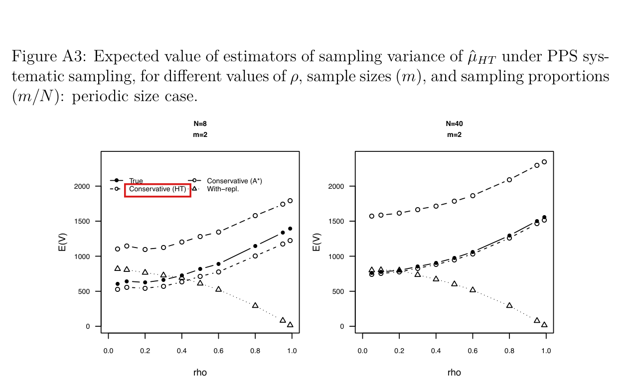
[Supplement, Section A, p. A1 (supplement PDF p. 1)] “In the simulations, expected values of $\widehat{\mathrm{Var}}(\hat t)$ and $\widehat{\mathrm{Var}}_C(\hat t)$ were computed exactly using expressions from Propositions 1 and 2 in the main text. Expected values for alternative estimators were computed using exact expressions for bias when available and via simulated sample draws otherwise. All simulations study expected values of estimators for the sampling variance of the Horvitz-Thompson estimator for the population mean, $$\hat\mu_{HT} \equiv \frac{1}{N}\hat t.$$” So in the supplement the estimand is $\mathrm{Var}(\hat\mu_{HT}) = \mathrm{Var}(\hat t)/N^2$ and the estimators are $(1/N^2)\widehat{\mathrm{Var}}(\hat t)$ and $(1/N^2)\widehat{\mathrm{Var}}_{C2}(\hat t)$; by Proposition 1 the bias of $(1/N^2)\widehat{\mathrm{Var}}(\hat t)$ is $A/N^2$.
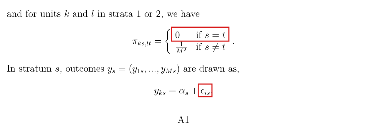
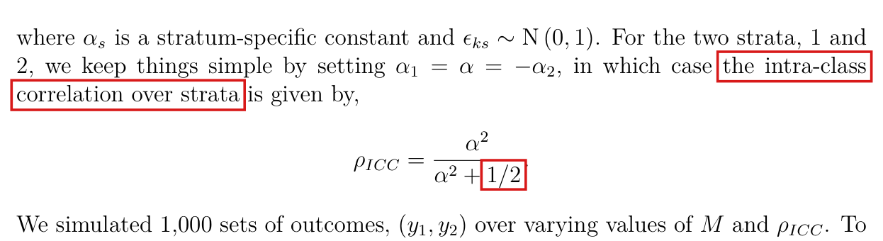
[Supplement, Section B, one unit per stratum: pp. A1–A2 (supplement PDF pp. 1–2)] “Simplifying that context, we consider two strata each of size $M$, in which case $N = 2M$. From each stratum a single unit is randomly sampled. Thus, for unit $k$ in stratum $s$, $$\pi_{ks} = \pi = \frac{1}{M},$$ and for units $k$ and $l$ in strata 1 or 2, we have $$\pi_{ks,lt} = \begin{cases} 0 & \text{if } s = t \\ \frac{1}{M^2} & \text{if } s \neq t \end{cases}.$$ In stratum $s$, outcomes $y_s = (y_{1s}, ..., y_{Ms})$ are drawn as, $$y_{ks} = \alpha_s + \epsilon_{is},$$ where $\alpha_s$ is a stratum-specific constant and $\epsilon_{ks} \sim \mathrm{N}(0, 1)$. For the two strata, 1 and 2, we keep things simple by setting $\alpha_1 = \alpha = -\alpha_2$, in which case the intra-class correlation over strata is given by, $$\rho_{ICC} = \frac{\alpha^2}{\alpha^2 + 1/2}.$$ We simulated 1,000 sets of outcomes, $(y_1, y_2)$ over varying values of $M$ and $\rho_{ICC}$. To each set, we applied the single-unit-per-stratum design. Then, we computed three approximations of the sampling variance of the Horvitz-Thompson estimator of the population mean: 1. The Horvitz-Thompson estimator for the sampling variance of the estimator for the population mean, $(1/N^2)\widehat{\mathrm{Var}}(\hat t)$. 2. The bias-adjusted estimator, $(1/N^2)\widehat{\mathrm{Var}}_{C2}(\hat t)$. 3. The “collapsed stratum” estimator (Wolter, 2007, 51-2), which for this case, given unit $k$ from stratum 1 and unit $l$ from stratum 2 selected into $s^0$, equals, $$\widehat V_{CS}(\hat\mu_{HT}) = \frac{1}{N^2}\left(\frac{y_{k1}}{\pi_1} - \frac{y_{l2}}{\pi_2}\right)^2 = \frac{1}{4}(y_{k1} - y_{l2})^2.$$” (The two misprints in these displays, the missing restriction to distinct units and $\epsilon_{is}$ for $\epsilon_{ks}$, are finding P027-E006; see P027-T18.) The supplement does not say that the errors $\epsilon_{ks}$ are independent, or that the two strata are sampled independently; both are the ordinary reading and are used by the validators.
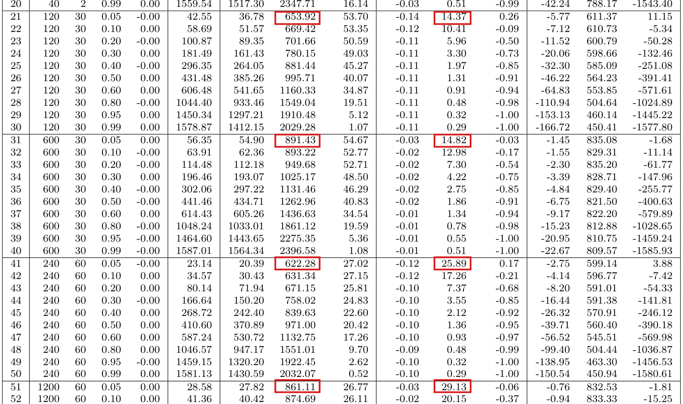
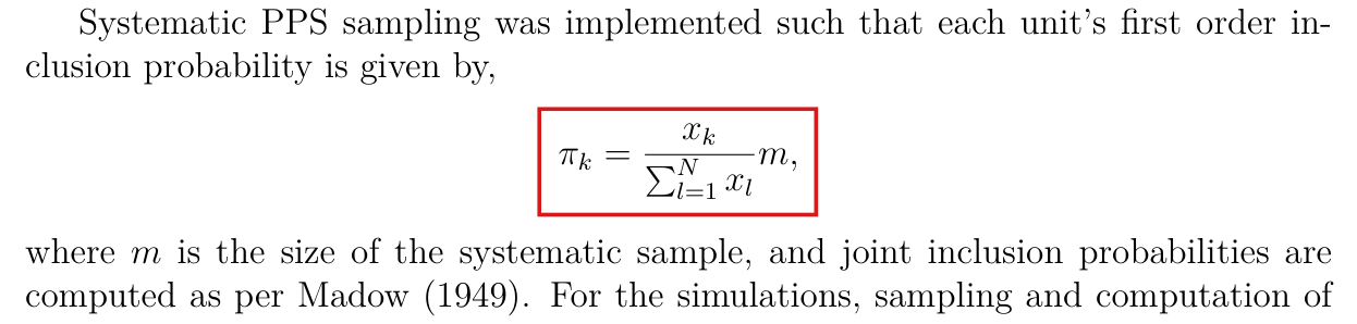
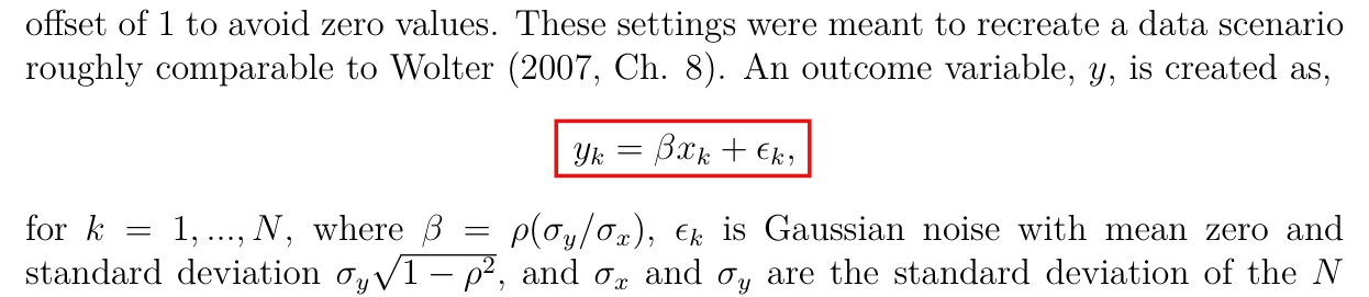
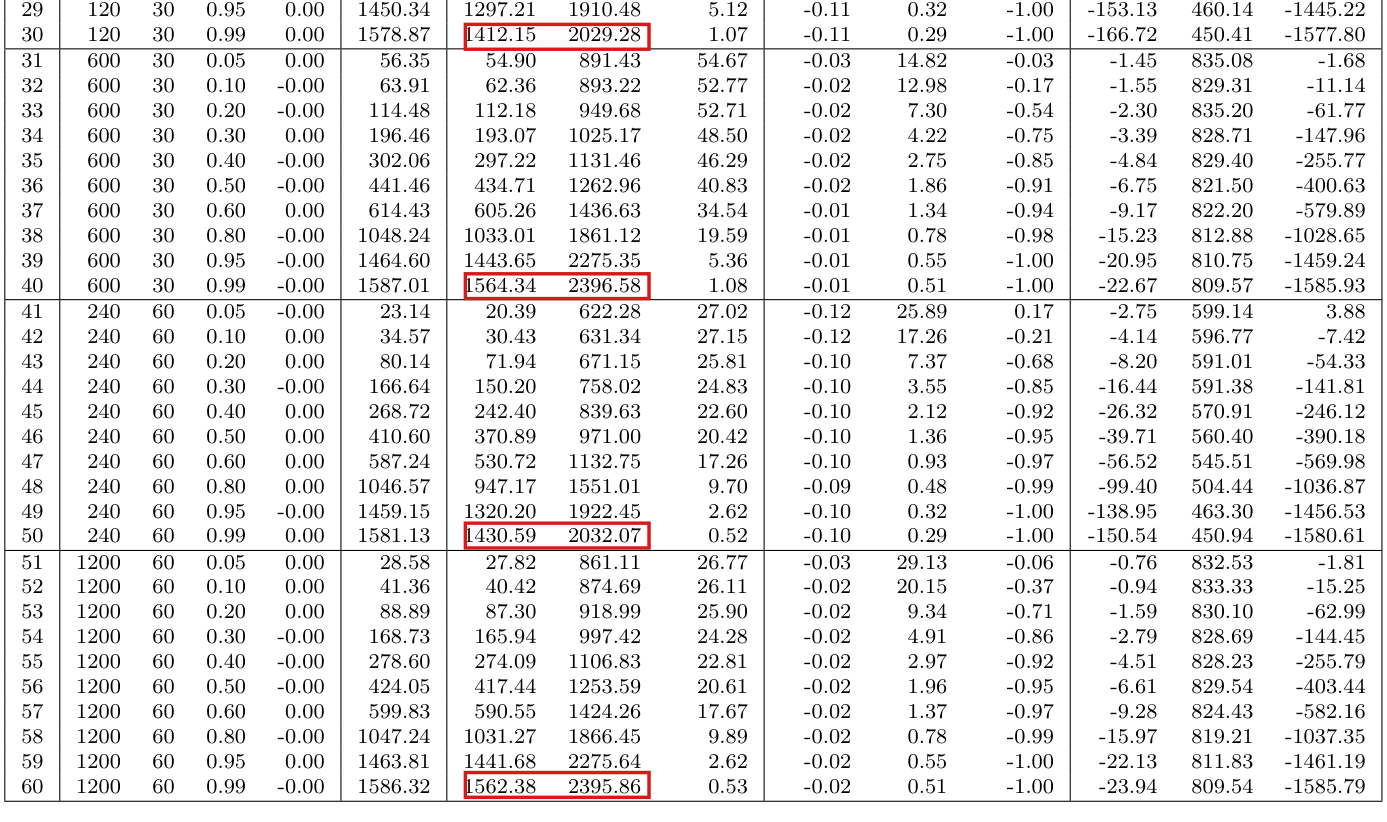
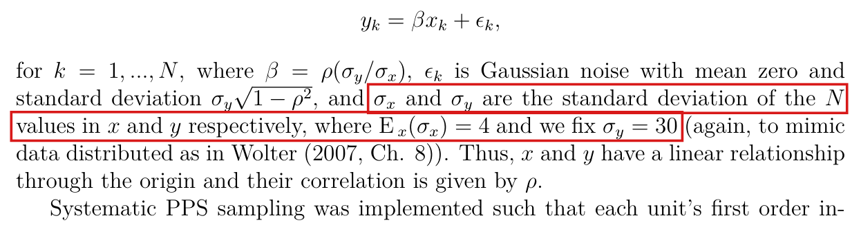
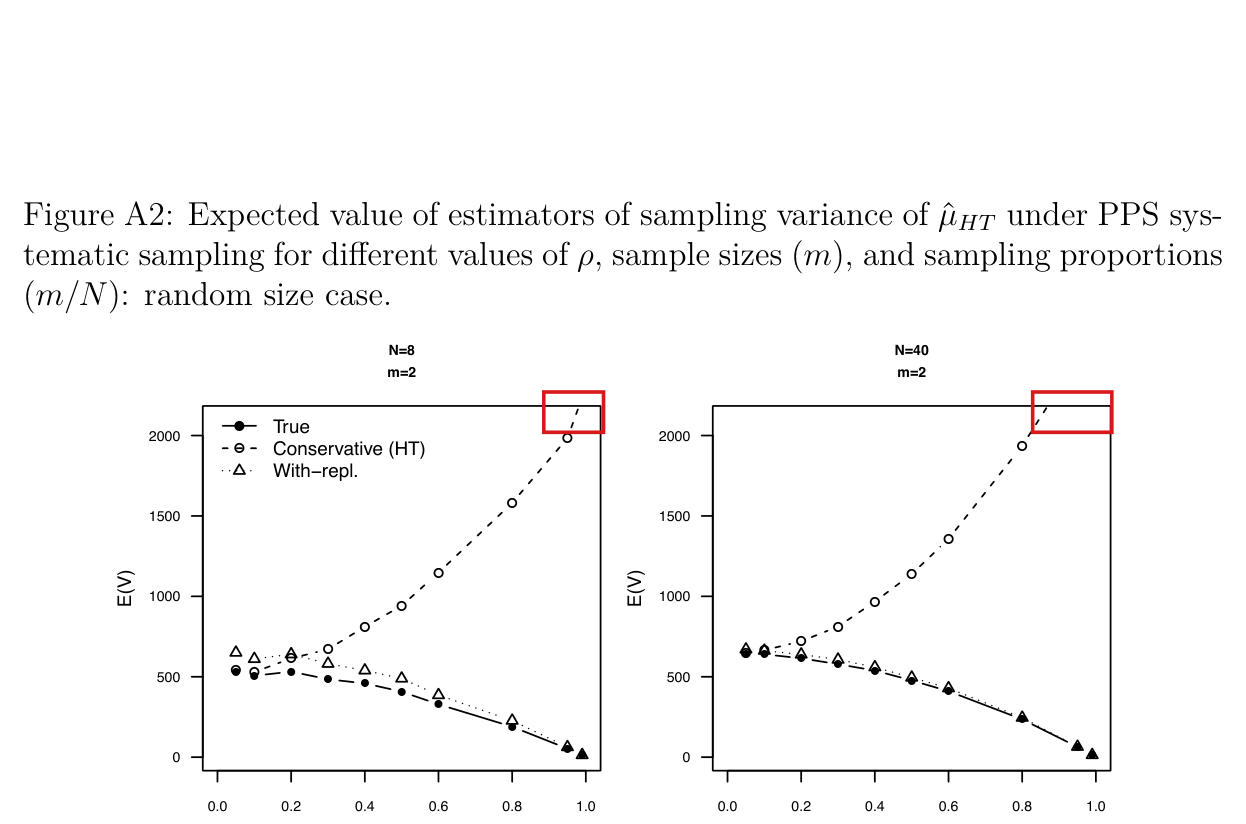
[Supplement, Section C, systematic PPS sampling: pp. A3–A4 (supplement PDF pp. 3–4)] “For the simulations, a size variable, $x = (x_1, ..., x_N)$, is produced as a vector of $N$ random draws from a negative binomial distribution with mean 6, variance 16, and offset of 1 to avoid zero values. These settings were meant to recreate a data scenario roughly comparable to Wolter (2007, Ch. 8). An outcome variable, $y$, is created as, $$y_k = \beta x_k + \epsilon_k,$$ for $k = 1, ..., N$, where $\beta = \rho(\sigma_y/\sigma_x)$, $\epsilon_k$ is Gaussian noise with mean zero and standard deviation $\sigma_y\sqrt{1 - \rho^2}$, and $\sigma_x$ and $\sigma_y$ are the standard deviation of the $N$ values in $x$ and $y$ respectively, where $\mathrm{E}_x(\sigma_x) = 4$ and we fix $\sigma_y = 30$ (again, to mimic data distributed as in Wolter (2007, Ch. 8)). Thus, $x$ and $y$ have a linear relationship through the origin and their correlation is given by $\rho$. Systematic PPS sampling was implemented such that each unit's first order inclusion probability is given by, $$\pi_k = \frac{x_k}{\sum_{l=1}^{N} x_l}m,$$ where $m$ is the size of the systematic sample, and joint inclusion probabilities are computed as per Madow (1949).” The with-replacement estimator (p. A3): $$\widehat{\mathrm{Var}}_{WR}(\hat\mu_{HT}) = \frac{1}{N^2 m(m - 1)}\sum_{k \in s^0}\left(\frac{y_k}{p_k} - \hat t\right)^2,$$ “where $p_k = \pi_k/m$ is the notional “per-draw” selection probability.” The periodic design (pp. A3–A4): “we performed a second set of simulations where the size variable, $x$, was drawn as an $N$-length vector of repeating 2's and 10's, thus maintaining variance values that are comparable to the previous simulation. Also, so that we could provide an illustration of the performance of $\widehat{\mathrm{Var}}_{C2}(\hat t)$, we produced $y_k$ values in the same manner as above, but then worked with the demeaned value, $$\tilde y_k \equiv y_k - \bar y,$$ as the variable with which $\hat\mu_{HT}$ was computed.” The supplement does not display the systematic selection rule; the validators and the targets below use the usual cumulative-size rule with one uniform random start (unit $k$ occupies the interval $[c_{k-1}, c_k)$ with $c_k = \sum_{a \le k} x_a$; with $I = \sum_l x_l/m$ and $u$ uniform on $[0, I)$ the sample is the set of units whose intervals contain $u, u + I, \ldots, u + (m-1)I$), and the order $x = (2, 10, 2, 10, \ldots)$. The $(N, m)$ pairs of Tables A2 and A3 (pp. A7–A8) are $(8, 2), (40, 2), (120, 30), (600, 30), (240, 60), (1200, 60)$, so $q = N/m \in \{4, 20\}$.
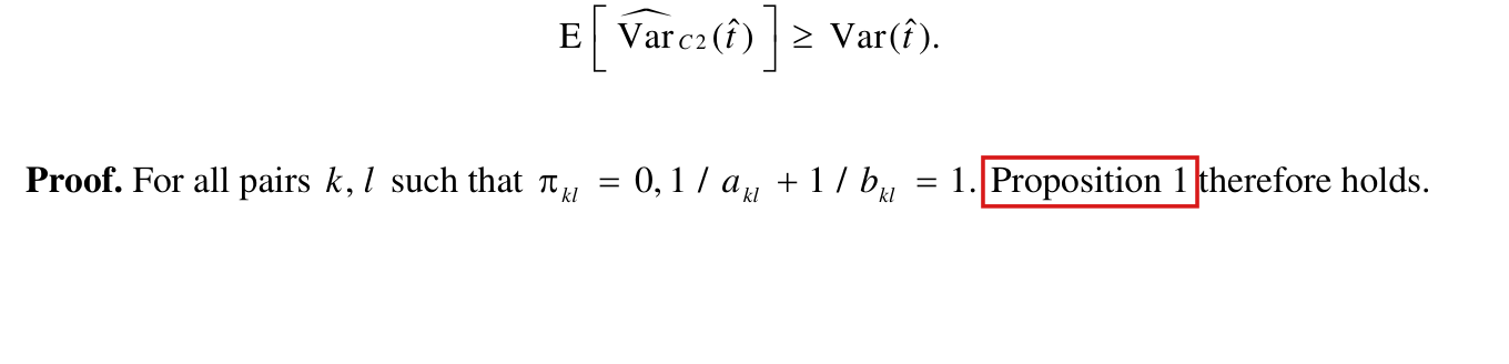
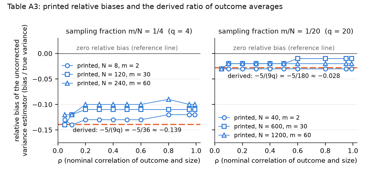
Effective claim (source TeX): Sol's repair (validated.json, P027-E004, smallest_repair), verbatim: "Replace the final cancellation explanation and qualify its accuracy claim: In this centered periodic design, the possible samples form q=N/m disjoint groups. Writing T_g for their outcome totals, the bias of the unadjusted mean-variance estimator is -sum_g T_g^2/N^2. Under independent Gaussian residuals as in the generating process, the ratio of outcome-averaged bias to outcome-averaged true variance is -5/(9q). Thus the estimator is relatively close at the smaller sampling fraction, but retains negative bias at either fixed sampling fraction; population demeaning does not cancel this bias. Optionally make the earlier general sign statement explicit by adding in general, or describe the local bias as nonpositive."
Mathematical content, with every hypothesis (validator's derivation.md, sections 2, 3 and 5).
Setting. $m \ge 1$ and $q \ge 2$ are integers with $q$ even, and $N = mq$ (Table A3 has $q \in \{4, 20\}$). Sizes: $x_k = 2$ for odd $k$ and $x_k = 10$ for even $k$, $k = 1, \ldots, N$; so $\sum_l x_l = 6N$. Design: systematic PPS sampling by cumulative sizes with one uniform start (unit $k$ occupies $[c_{k-1}, c_k)$, $c_k = \sum_{a \le k} x_a$; $u$ is uniform on $[0, 6q)$; the sample is the set of units whose intervals contain $u + 6qj$, $j = 0, \ldots, m - 1$). Outcomes: any real vector $z = (z_1, \ldots, z_N)$ with $\sum_k z_k = 0$ (the demeaned $\tilde y$ of the supplement); (i)–(iv) use nothing else about $z$.
(i) [The design.] The possible samples are the $q$ sets $G_g = \{g, g + q, \ldots, g + (m-1)q\}$, $g = 1, \ldots, q$; they partition $U$; $G_g$ is drawn with probability $p_g = 1/(3q)$ for odd $g$ and $p_g = 5/(3q)$ for even $g$. Hence $\pi_k = p_g = m x_k/\sum_l x_l$ for $k \in G_g$; $\pi_{kl} = p_g$ when $k, l \in G_g$ (including $k = l$); and $\pi_{kl} = 0$ when $k$ and $l$ lie in different sets.
(ii) [The bias term.] With $T_g = \sum_{k \in G_g} z_k$, $$A = \sum_{g}\sum_{h \ne g} T_g T_h = \Big(\sum_g T_g\Big)^2 - \sum_g T_g^2 = -\sum_{g=1}^{q} T_g^2 \le 0,$$ with $A = 0$ if and only if $T_g = 0$ for every $g$.
(iii) [Variance and expected estimator.] $\mathrm{E}(\hat t) = 0$ and $\mathrm{Var}(\hat t) = \sum_g T_g^2/p_g$. When $G_g$ is drawn, $\widehat{\mathrm{Var}}(\hat t) = (1 - p_g)T_g^2/p_g^2$. Hence $$\mathrm{E}\big[\widehat{\mathrm{Var}}(\hat t)\big] = \sum_g\Big(\frac{1}{p_g} - 1\Big)T_g^2 = \mathrm{Var}(\hat t) - \sum_g T_g^2,$$ and the bias of $(1/N^2)\widehat{\mathrm{Var}}(\hat t)$ as an estimator of $\mathrm{Var}(\hat\mu_{HT})$ is $-\sum_g T_g^2/N^2$: it is never positive, and it is zero only if every sample total is zero.
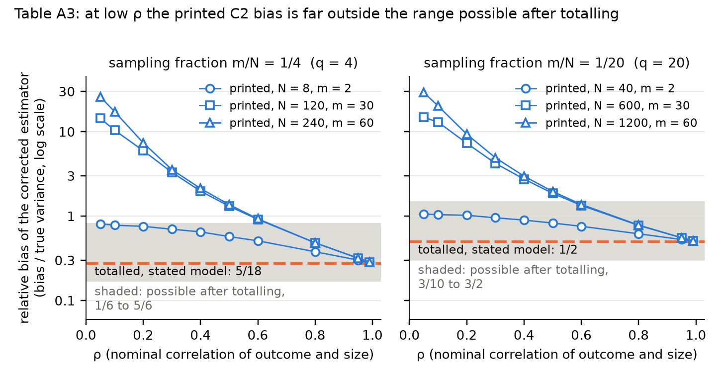
(iv) [Size of the relative bias for a fixed population.] If $\mathrm{Var}(\hat t) > 0$, then $$-\frac{5}{3q} \le \frac{A}{\mathrm{Var}(\hat t)} \le -\frac{1}{3q}.$$
(v) [Under the outcome model, second moments only.] Let $z_k = y_k - \bar y$ with $y_k = \beta x_k + \epsilon_k$, where $\beta$ is a real constant and $\epsilon_1, \ldots, \epsilon_N$ are random variables with mean zero, common variance $\tau^2$ and zero covariances (in the supplement they are independent Gaussian with $\tau^2 = \sigma_y^2(1 - \rho^2) = 900(1 - \rho^2)$). Write $\mathrm{E}_y$ for expectation over the $\epsilon_k$. Then for every $g$, $$\mathrm{E}_y(T_g^2) = 16 m^2\beta^2 + m\tau^2\Big(1 - \frac{1}{q}\Big) =: D,$$ $\mathrm{E}_y(A) = -qD$ and $\mathrm{E}_y(\mathrm{Var}(\hat t)) = \tfrac{9}{5}q^2 D$. Hence, when $D > 0$, $$\frac{\mathrm{E}_y\big(\mathrm{E}[\widehat{\mathrm{Var}}(\hat t)] - \mathrm{Var}(\hat t)\big)}{\mathrm{E}_y\big(\mathrm{Var}(\hat t)\big)} = -\frac{5}{9q},$$ that is $-5/36$ for $q = 4$ and $-1/36$ for $q = 20$, for every $N$, $\beta$ and $\tau$; the same ratio holds on the mean scale. This is a ratio of outcome-averaged quantities; it is not the relative bias of each realized population (compare (iv)).
(vi) [Fixed sampling fraction.] $\mathrm{E}_y(A/N^2) = -16\beta^2/q - \tau^2(1 - 1/q)/N$. With the supplement's $\beta = \rho\,\sigma_y/\sigma_x$, $\sigma_y = 30$, and $\sigma_x^2 = 16N/(N-1)$ (the divisor-$(N-1)$ variance of the periodic sizes), this is $$\mathrm{E}_y\Big(\frac{A}{N^2}\Big) = -900\rho^2\,\frac{N-1}{qN} - 900(1 - \rho^2)\,\frac{q - 1}{qN},$$ which for fixed $q$ and $\rho \ne 0$ is bounded away from $0$ for all $N$ and has limit $-900\rho^2/q$ as $N \to \infty$ ($-220.5225$ at $q = 4$, $\rho = 0.99$).
Corrected passage: in this centered periodic design the uncorrected estimator is close to the true variance in relative terms when $q$ is large (relative bias between $-5/(3q)$ and $-1/(3q)$), but it is biased downward at each fixed sampling fraction; demeaning the outcomes does not make the elements of $A$ cancel.
: SAP.P027a.T2WholeStatement
Theorem: SAP.P027a.T2
Statement hash: 1438004a9d4de9210cfdba7ce53c0b34ec52a8ce13e8d204b1dc6229c1fbf6f2
Statement definition: SAP.P027a.T2WholeStatement
Certificate. 20261104T181735Z
Declaration review: faithful; 2026-11-04T18:41:50Z; binding v2
Evidence scope: Certification checks formal proof objects. Statement fidelity is a model judgment. Author review is separate.
Proof dependencies: Independently extracted
Manifest annotation reconciliation: Effective use follows the source-bound dependency observation; original annotations are retained in the crosswalk.
AronowAudit.P027.centered_cross_products: observed used
AronowAudit.P027.centered_outcomes_linear: observed used
AronowAudit.P027.centered_outcomes_zero: observed used
AronowAudit.P027.centered_unit_second_moment: observed used
AronowAudit.P027.centering_coeff_square_sum: observed used
AronowAudit.P027.noise_linear_moments: observed used
AronowAudit.P027.oneDraw_centered_variance: observed used
AronowAudit.P027.oneDraw_ht_estimator: observed used
AronowAudit.P027.oneDraw_joint: observed used
AronowAudit.P027.oneDraw_pi: observed used
AronowAudit.P027.oneDraw_total: observed used
AronowAudit.P027.periodic_ht_expectations: observed used
AronowAudit.P027.periodic_model_bias: observed used
AronowAudit.P027.periodic_negative_square: observed used
AronowAudit.P027.periodic_size_moments: observed used
AronowAudit.P027.phaseGrouped_positive: observed used
AronowAudit.P027.phase_centered_total_formula: observed used
AronowAudit.P027.phase_inverse_sum: observed used
AronowAudit.P027.phase_noise_coeff_square_sum: observed used
AronowAudit.P027.phase_zero_degree: observed used
AronowAudit.P027.sum_ne_const: observed used
Source and evidence metadata · sap-2026-11-08-assured-release











My comment and the history of this entry
Suggested classification: Minor error.
My position My comment above; I suggested a Minor error.
The models’ position The supplement does not explain its departure from the preprocessing that the main text recommends, so the reported simulations cannot evaluate the recommended procedure; in highlighted rows they differ from its possible bias by one to two orders of magnitude: Moderate.