LLM-generated corrections to the published research of P. M. Aronow

Journal article P032

Corrections to: Dyadic Clustering in International Relations

Jacob Carlson, Trevor Incerti, and P. M. Aronow (2024). Dyadic Clustering in International Relations. Political Analysis 32(2):186–198.

DOI
10.1017/pan.2023.26
arXiv
2109.03774
Audited edition
Political Analysis, 2024, 32(2):186–198; 13 pages in the audited file
SHA-256 of the audited file
69493a1fc4a2706339bfaeb01af78aae7fa76cce7bb3f5f990468edf88d94a15
Permanent address
https://pmaronow.github.io/llm-audit/works/P032/

Summary

The article asks how much dyadic clustering affects inference in international relations. It reanalyzes 22 dyadic studies from International Organization (January 2014 to January 2020) with dyadic clustering robust standard errors (DCRSEs), and reports that DCRSEs average 1.74 times the original standard errors and that 67% of significant estimates remain significant. 16 entries are classified as errors (5 Moderate, 11 Minor, none Major or Critical), and 3 are clarity notes. The most consequential is P032-N004: for 13 survival models behind two study rows, the Stata command does not subtract the matrix V^0\widehat V_0 that the decomposition on p. 191 requires, and those rows have not been recomputed.

What was and was not checked

I examined the article (13 pages), its Supplementary Appendix (5 pages) and the replication files. These are the Dataverse package, with its code, the outputs that it saves for each model and data from six of the 22 studies, and the R and Stata packages dcr. The list below states what was examined and held up. It is not a finding that the rest of the article is correct.

  • The decomposition. The identity V^r=∑i=1NV^c,i−V^D−(N−2)V^0\widehat V_r=\sum_{i=1}^{N}\widehat V_{c,i}-\widehat V_D-(N-2)\widehat V_0 on p. 191 holds by a counting argument, and exactly on small designs with repeated and reversed dyads. It requires that each dyad has two distinct members, that NN is the number of dyad members, and that V^c,i\widehat V_{c,i} clusters the observations containing member ii and treats every other observation as its own cluster (see P032-N005 and P032-N003). In the 35 models checked against a direct computation, the decomposition equals the direct sum over pairs of observations whose dyads share a member: 9 regressions of Shelef (2016), 21 probits of Copelovitch and Putnam (2014) and 5 models of Pratt (2018).
  • The software on the models re-estimated. For the two Stata studies among these, the saved DCRSEs and original standard errors agree with a separate computation in R to at least five significant digits, and the R function reproduces a direct computation for the five models of Pratt (2018). Three models of Arel-Bundock (2017) were also refitted from the replication data, and their study row agrees with Table A.2 after rounding. The factors that remove the finite-sample corrections are right for regress and for the maximum-likelihood commands. The copies of dcr.ado and nclogit.ado in the Dataverse package and in the Stata package are identical. Other parts of the two packages are the subject of P032-E004, P032-E005, P032-E006, P032-N004 and P032-N010.
  • Table 5 and Supplementary Table A.2. I rebuilt the 20 rows of Table A.2 for the studies analyzed in Stata and its average row (0.455, 0.224, 0.046, 0.276, 1.743) from the saved outputs. With the two rows for the studies analyzed in R taken as printed, every cell of Table 5 follows, and its 77 numeric cells agree after rounding. In all 7,782 saved coefficient rows, the standard error ratio and the normal pp-values agree with the saved standard errors to within 3.4×10−163.4\times10^{-16}. This checks the arithmetic and not the fitted models.
  • The text against the tables. The values 1.74, 0.22 and 0.05 agree with Table 5, and the 67% equals 0.455/(0.455+0.224)0.455/(0.455+0.224). The range 0.90 to 4.16, the 18 of 22 studies whose standard error ratio is above 1 on average and the 7 of 22 with no loss of significance agree with Supplementary Table A.2, and the subfield statements on pp. 193 and 196 agree with Table 5. The counts agree with the code: 174 models, 24 models in three studies without robust or clustered standard errors, and 20 state-dyad and 2 IO-dyad studies. Inverse study frequency weighting is an average of study averages, as footnote 14 says. The number of studies in which half or more of the key explanatory variables (KEVs) become insignificant is the subject of P032-E002, and the count of 691 KEVs is the subject of P032-E008.
  • Section 2 and Tables 1–4. The variance algebra of Section 2.1 and the dependence patterns of Table 1 are correct, and the zero patterns of Tables 2–4 are right for the labels as printed (P032-N003).
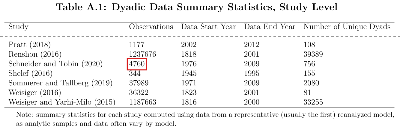
  • The supplementary tables. The rows of Table A.1 for Copelovitch and Putnam (2014), Powell (2015), Pratt (2018) and Shelef (2016) equal the estimation samples in the data. The row for Schneider and Tobin (2020) is the subject of P032-N011. The rows of Table A.4 are the primary results for the models listed (P032-N006 concerns the classification of one study). The “All” row of Table A.5 is consistent with its year and subfield rows, I rebuilt the year rows for 2014, 2015, 2016, 2019 and 2020, and the table is close to Table 5 (1.75 against 1.74). The correction of the original standard errors in that table is the subject of P032-E011.
  • Figures and other points. The published Figures 1–3 agree on visual comparison with the figures saved in the replication files (the note to Figure 3 is the subject of P032-E010). The scripts for the small-sample reanalysis differ from the primary ones only in the option for the correction, the output paths and the reference distribution. The ordered probit used in place of a probit for one model of Colgan (2014) leaves the slopes and their standard errors unchanged. I read all supplementary pages, footnotes and references.

The following were not checked, or could not be.

  • Stata was not available. I examined the Stata command by reading it and by reproducing its saved output in R for two studies, and ran none of the Stata models.
  • Twenty data files of the Dataverse package, those larger than 5 MB or inside nested archives, were not read in the initial examination. With Arel-Bundock (2017) also refitted in the separate reproduction, data from 16 of the 22 studies were not examined, and those studies were checked only through the saved outputs.
  • The following were not re-estimated: one model of Pratt (2018) fitted with arm::bayesglm, the multinomial logit of Powell (2015) and the multiple-imputation logit of Schneider and Tobin (2020). The two R-study rows of Table A.2 were taken as printed for the complete Table 5 recalculation; the Pratt (2018) row could not be fully checked by refitting.
  • The 22 reanalyzed articles were not available. The published standard errors and significance markers could not be compared with the re-estimated ones, and whether four estimates of Carter and Poast (2020) were published as significant at the 5% level could not be determined. The search that returned 70 studies and the exclusions from it could not be examined.
  • The statement on p. 196 that the failure to compute DCRSEs “does not appear to have led to systematically false substantive conclusions” was not assessed. The arithmetic of retained significance behind it holds, and the sources contain nothing on whether the conclusions of the 22 studies are true.
  • No published correction to the article is among the sources, and I did not search for one elsewhere.

Headline claims and related corrections

  1. Standard errors from the studies' original variance estimators are on average about half as large as DCRSEs (equivalently DCRSEs are about twice as large); the inverse-study-frequency-weighted (ISFW) average standard error ratio is 1.74.

    Abstract; pp. 187, 193, 196; Table 5 row 'All'; Supplementary Table A.2; Figure 1

    See P032-N004, P032-E004, P032-E008, P032-N007.

  2. Most (67%, 'two-thirds') of the statistically significant key explanatory variable estimates remain significant at the 5% level with DCRSEs.

    Abstract; pp. 187, 196; Table 5 row 'All' (0.46 and 0.22); Supplementary Table A.2 last row (0.455, 0.224); Figures 2-3

    See P032-N004, P032-E004, P032-E008.

  3. The ISFW proportion of KEVs going from significant to insignificant is 0.22, and a small proportion (0.05) go from insignificant to significant, which the paper attributes to sampling variability of the standard error estimators.

    p. 193; Table 5 row 'All'

  4. No subfield is immune: every subfield has an average SER above 1.5 and at least 19% of estimates losing significance; in IOs/International Law DCRSEs are on average more than twice the original SEs and 34% of estimates become insignificant.

    pp. 193, 196; Table 5 subfield rows

    See P032-N004.

  5. Study-level average SERs range from 0.90 to 4.16; 18 of 22 studies are less precise with DCRSEs; only 7 of 22 lose no significant KEV; three studies see half or more of their KEVs become insignificant.

    p. 196; Supplementary Table A.2

    See P032-E002, P032-N004.

  6. The reanalysis covers all International Organization articles from January 2014 to January 2020 with dyadic data that meet the inclusion rules: 22 studies, 174 models, 691 KEVs; 24 models in three studies used no robust or clustered SE; three studies have a model with fixed effects for both dyad members; 20 studies use state dyads and 2 use IO dyads.

    p. 192 and footnotes 8-10; Supplementary Tables A.1, A.3, A.4

    See P032-E009, P032-E008, P032-N006, P032-N011.

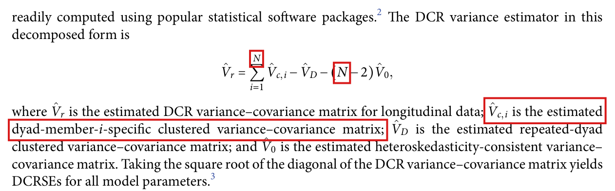
  7. The DCR variance estimator can be computed as V^r=∑iV^c,i−V^D−(N−2)V^0\hat V_r=\sum_i\hat V_{c,i}-\hat V_D-(N-2)\hat V_0, using member-specific clustered, repeated-dyad clustered and heteroskedasticity-consistent estimators. The R and Stata packages implement DCRSEs for the models in the reanalysis.

    Section 3 display (p. 191); abstract; pp. 187, 196; Data Availability Statement; supplement p. A1; packages dcr (R) and dcr (Stata)

    See P032-N004, P032-E004, P032-E005, P032-E006, P032-N005, P032-N003, P032-N010, P032-N012.

  8. Repeating the reanalysis with a small-sample correction gives no substantive differences from the primary reanalysis.

    Footnote 12, p. 193; Supplementary Table A.5

    See P032-E011.

  9. Dyads sharing a member can be dependent in ways that clustering only on repeated dyads misses. In the additive example, ignoring this dependence understates the variance of the average of two dyadic outcomes by (ac/2)Var⁡(XUS)(ac/2)\operatorname{Var}(X_{US}) when aa and cc have the same sign.

    Section 2.1 displays (pp. 188-189); Table 1; Tables 2-4

    See P032-N003.

  10. The reanalysis supplies a lower bound on the consequences of inadequate clustering because dependence between non-incident dyads further increases uncertainty.

    pp. 187, 191, 196; Section 3 sandwich variance expression and Table 4 dependence restriction

    See P032-E001.

  11. Failure to account for dyadic clustering has not apparently produced systematically false substantive conclusions, although it substantially overstates precision.

    Conclusion, p. 196; Table 5; Table A.2; Figures 2-3

Corrections

Moderate (5)

A real substantive error with limited reach.

Under dependence between non-incident dyads, DCRSEs can overstate uncertainty as well as understate it, and the reanalysis is a lower bound on the consequences of inadequate clustering only under a sign condition that the article does not state.

Introduction, paragraph beginning “Note, however”, p. 187 (PDF p. 2); Section 3, paragraph beginning “Note that the above approach”, p. 191 (PDF p. 6); Conclusion, first paragraph, p. 196 (PDF p. 11)

See also under Formal statements (Lean): P032-T1, P032-T2, P032-T5

My comment on this entry

As printed

Page 187. When there is dependence between non-incident dyads (i.e., dyads that do not share a common member), DCRSEs will still underestimate uncertainty, just as only clustering on repeated dyads underestimates uncertainty when there is dependence across incident dyads. DCRSEs should therefore not be considered a replacement for approaches to clustering that (appropriately) account for greater amounts of dependence in the data. The reanalysis we present therefore offers a lower bound on the severity of the consequences of inadequate clustering practices in previous research, or, in other words, reveals the extent to which dyadic clustering alone is jeopardizing the reliability of research.

Page 191. DCRSEs are not sufficient—although still improve over the naive approach or clustering by repeated dyad approach—when there are interdependencies throughout the entire system (i.e., across non-incident dyads). … Aronow et al. (2018) developed conservative estimators for the variance of least squares estimators in such cases where there is further dependence—and in such cases we expect the variance of least squares estimates to be larger than those that only take into account dyadic clustering.

Page 196. We investigated the consequences of failing to account for dyadic clustering in previous empirical research by reanalyzing all quantitative dyadic analyses in International Organization published in a 6-year window, thereby revealing a lower bound on the severity of the consequences of inadequate clustering practices in previous quantitative dyadic research.

The problem

The passage on p. 187 states a direction: when non-incident dyads are dependent, DCRSEs underestimate uncertainty. From this direction the article infers that its reanalysis is a lower bound on the consequences of inadequate clustering, and the Conclusion repeats the inference. The direction does not hold in general. The DCR variance estimator treats as zero the covariances between observations whose dyads share no member. In the variance of an estimated coefficient, each omitted covariance is weighted by the product of the weights of its two observations, and the sum of these weighted terms can be positive, zero or negative. When the sum is negative, the true variance of the estimated coefficient is smaller than the population dyadic sandwich value, and DCRSEs can overstate uncertainty. The article states no condition on the sign of the sum. The condition in Section 2.1, that aa and cc are of the same sign, belongs to the toy example. A positive covariance between the errors of non-incident dyads is also not enough, since the weights of two observations in a slope can have opposite signs. Without a sign condition, the comparison of DCRSEs with the original standard errors measures the effect of dyadic clustering and bounds the effect of further dependence in neither direction. The expectation of a larger variance on p. 191 requires a positive omitted weighted covariance sum; the aside there that DCRSEs still improve over the naive approach is not guaranteed.

Evidence an exact counterexample

The evidence is a derivation and six exact examples. Let XX be a fixed n×pn\times p matrix of full column rank, and let Y=Xβ+uY=X\beta+u with E[u]=0\mathbb{E}[u]=0 and E[uuT]=Ω\mathbb{E}[uu^T]=\Omega. Fix c∈Rpc\in\mathbb{R}^p and set h=X(XTX)−1ch=X(X^TX)^{-1}c. Since β^−β=(XTX)−1XTu\widehat\beta-\beta=(X^TX)^{-1}X^Tu, I have cTβ^−cTβ=hTuc^T\widehat\beta-c^T\beta=h^Tu, and the true variance is V=Var⁡(cTβ^)=hTΩhV=\operatorname{Var}(c^T\widehat\beta)=h^T\Omega h. Let drd_r denote the dyad of observation rr, and let ΩD\Omega_D impose the restriction of Table 4, with entries (ΩD)rs=Ωrs(\Omega_D)_{rs}=\Omega_{rs} if dr∩ds≠∅d_r\cap d_s\neq\varnothing and (ΩD)rs=0(\Omega_D)_{rs}=0 otherwise. The population dyadic sandwich value is VD=hTΩDhV_D=h^T\Omega_Dh. Subtracting, I obtain

V−VD=hT(Ω−ΩD)h=∑(r,s): dr∩ds=∅hrhsΩrs,V-V_D=h^T(\Omega-\Omega_D)h=\sum_{(r,s):\,d_r\cap d_s=\varnothing}h_rh_s\Omega_{rs},

where the sum is over ordered pairs of observations. I denote this sum by Δ\Delta. This identity implies that VD≤VV_D\le V if and only if Δ≥0\Delta\ge0. Note that positive definiteness of Ω\Omega does not restrict the sign of Δ\Delta.

Examples 1 to 3 have two observations, on two dyads with no common member. In Examples 1 and 3 the coefficient is the intercept, with h=(1/2,1/2)Th=(1/2,1/2)^T. In Example 2 it is the slope on the single regressor x=(−1,1)Tx=(-1,1)^T, with h=(−1/2,1/2)Th=(-1/2,1/2)^T. Example 4 has one observation on each of the six dyads among four members, and Examples 5 and 6 have one observation on each of the dyads (A,B)(A,B), (A,C)(A,C), (D,E)(D,E) and (D,F)(D,F). In Examples 4 to 6 the coefficient is the intercept. Every error has variance 1. In Examples 1 to 5 the matrix Ω\Omega is positive definite, and in Example 6 it is the covariance matrix of an explicit distribution.

The true variance VV, the variance VDV_D with the covariances of non-incident dyads set to zero, and Δ=V−VD\Delta=V-V_D.
ExampleCovariances between observationsVVVDV_DΔ\Delta
1non-incident −1/2-1/21/41/41/21/2−1/4-1/4
2non-incident 1/21/21/41/41/21/2−1/4-1/4
3non-incident 1/21/23/43/41/21/21/41/4
4incident 1/81/8, non-incident −1/2-1/21/61/61/41/4−1/12-1/12
5incident 1/41/4, non-incident −1/4-1/43/163/165/165/16−1/8-1/8
6incident 1/41/4, non-incident 1/41/47/167/165/165/161/81/8

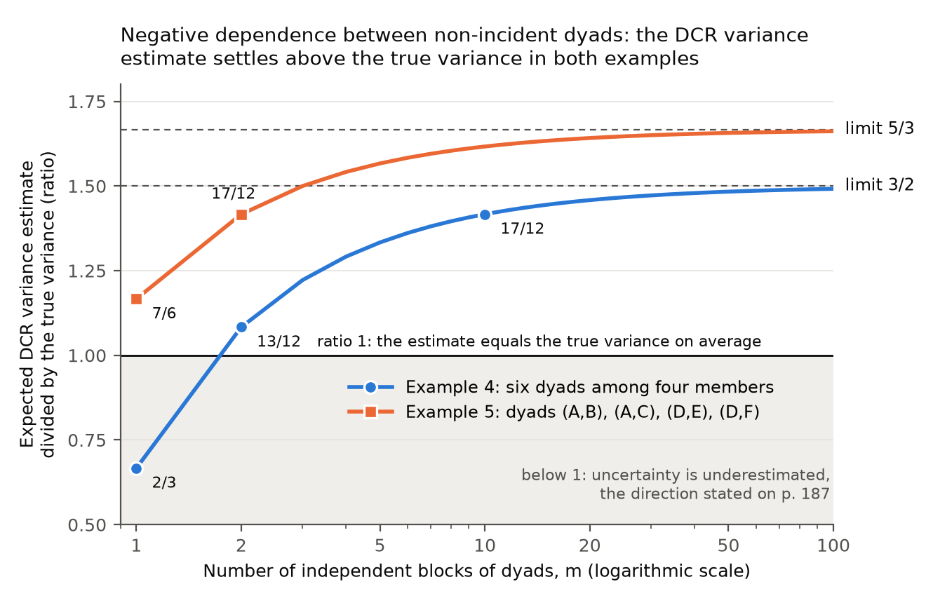
Examples 1, 2, 4 and 5 have V<VDV<V_D. Example 2 has a positive covariance between the two errors, and Examples 4 and 5 have positive dependence between incident dyads. Examples 3 and 6 show that the other direction also occurs.

The fitted estimator also overstates variance in the limit. In Example 4 the errors can be built from independent signs and are bounded. For mm independent copies of this block on disjoint members, I have n=6mn=6m and V=1/nV=1/n, and the DCR variance estimator, computed from residuals without a small-sample correction, has expectation 3/(2n)−5/n23/(2n)-5/n^2. The ratio of this expectation to VV is 3/2−5/n3/2-5/n, which equals 2/32/3 for m=1m=1, 13/1213/12 for m=2m=2 and 17/1217/12 for m=10m=10. By the law of large numbers, the ratio of the estimator to VV converges to 3/23/2. For mm independent copies of Example 5, I have V=3/(16m)V=3/(16m), and the estimator has expectation (10m−3)/(32m2)(10m-3)/(32m^2), which exceeds VV for every m≥1m\ge1. The ratio of the estimator to VV converges in probability to 5/35/3. In the limit, DCRSEs exceed the standard deviation of the estimate by the factors 3/2\sqrt{3/2} and 5/3\sqrt{5/3}. In Example 4 the variance with every covariance between distinct observations set to zero, as under the naive approach, equals VV. In Example 5 it is 1/41/4, which lies between V=3/16V=3/16 and VD=5/16V_D=5/16.

What survives

The toy example of Section 2.1 with its condition on the signs of aa and cc, the sandwich identity, the restriction of Table 4 and the decomposition on p. 191 are unaffected. The ratios of DCRSEs to the original standard errors, the comparisons of pp-values and the software do not use the direction of the omitted dependence, and this finding changes none of them. I have not independently recalculated those reported values. The sentence in the third paragraph of the Conclusion, that the problem “may be even more severe”, is correct as a statement of possibility (Examples 3 and 6). What changes is the interpretation. The reanalysis is not shown to be a lower bound. A population variance lower bound requires Δ≥0\Delta\ge0 for each coefficient, which has not been examined for the 22 studies. The result of Aronow, Crawford and Zubizarreta (2018) cited on p. 191 is not in question.

Corrected

Page 187. When there is dependence between non-incident dyads (i.e., dyads that do not share a common member), DCRSEs may still underestimate uncertainty, just as only clustering on repeated dyads may underestimate uncertainty when there is dependence across incident dyads. Non-incident dependence can also lower the sampling variance of a coefficient relative to the population dyadic sandwich value, so DCRSEs can overestimate uncertainty. DCRSEs should therefore not be considered a replacement for approaches to clustering that (appropriately) account for greater amounts of dependence in the data. The reanalysis compares DCRSEs with the standard errors from the original variance estimation strategies and documents the resulting changes in standard errors and statistical significance.

The condition. Let XX be a fixed n×pn\times p design matrix of full column rank, let Y=Xβ+uY=X\beta+u with E[u]=0\mathbb{E}[u]=0 and E[uuT]=Ω\mathbb{E}[uu^T]=\Omega, and let β^\widehat\beta be the least squares estimator. Fix c∈Rpc\in\mathbb{R}^p and set h=X(XTX)−1ch=X(X^TX)^{-1}c. Let drd_r be the dyad of observation rr, and let ΩD\Omega_D have entries (ΩD)rs=Ωrs(\Omega_D)_{rs}=\Omega_{rs} if dr∩ds≠∅d_r\cap d_s\neq\varnothing and (ΩD)rs=0(\Omega_D)_{rs}=0 otherwise. Then

Var⁡(cTβ^)−hTΩDh=∑(r,s): dr∩ds=∅hrhsΩrs,\operatorname{Var}(c^T\widehat\beta)-h^T\Omega_Dh=\sum_{(r,s):\,d_r\cap d_s=\varnothing}h_rh_s\Omega_{rs},

where the sum is over ordered pairs of observations. If this sum is nonnegative, then hTΩDh≤Var⁡(cTβ^)h^T\Omega_Dh\le\operatorname{Var}(c^T\widehat\beta). If it is positive, the inequality is strict. If it is negative, then hTΩDh>Var⁡(cTβ^)h^T\Omega_Dh>\operatorname{Var}(c^T\widehat\beta). The statement compares the variance of cTβ^c^T\widehat\beta with the population dyadic sandwich value. It does not order the estimates computed from residuals in every sample.

Page 191. DCRSEs are not sufficient when there are interdependencies throughout the entire system (i.e., across non-incident dyads), and an improvement over the naive approach or clustering by repeated dyad approach is not guaranteed. … Aronow et al. (2018) developed conservative estimators for the variance of least squares estimators in such cases where there is further dependence—and in such cases the variance of least squares estimates is larger than the population dyadic sandwich value when the sum above is positive for the coefficient, and smaller when it is negative.

Page 196. … by reanalyzing all quantitative dyadic analyses in International Organization published in a 6-year window, thereby documenting how standard errors and statistical significance change when DCRSEs are used. Without a justified sign for each coefficient’s omitted weighted covariance sum, the reanalysis is not a lower bound on the consequences of all inadequately modeled dependence.
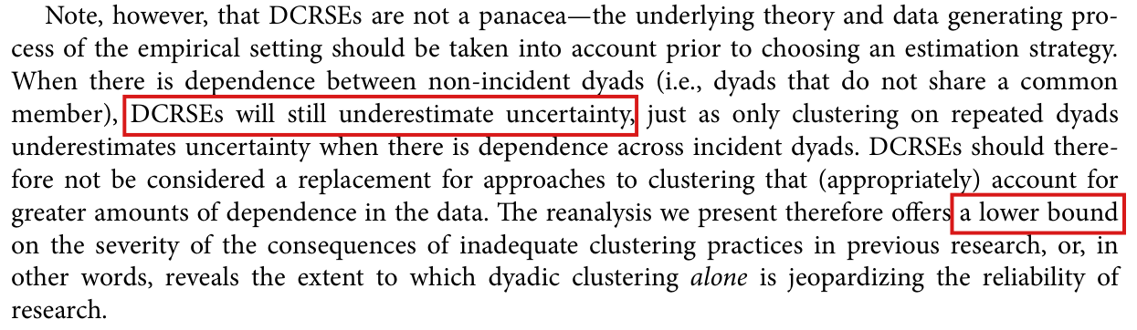
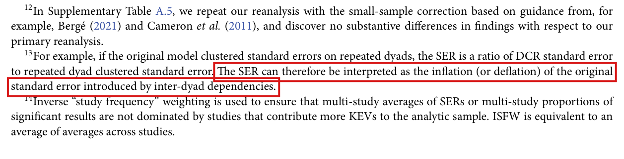
A paragraph of ten lines from the Introduction. A red box in the fourth line surrounds the words 'DCRSEs will still underestimate uncertainty'. A second red box at the end of the seventh line surrounds 'a lower bound', in the sentence 'The reanalysis we present therefore offers a lower bound on the severity of the consequences of inadequate clustering practices in previous research'.
Introduction, paragraph beginning “Note, however”, p. 187 (PDF p. 2). The marks are on the statement that DCRSEs “will still underestimate uncertainty” and on “a lower bound”.
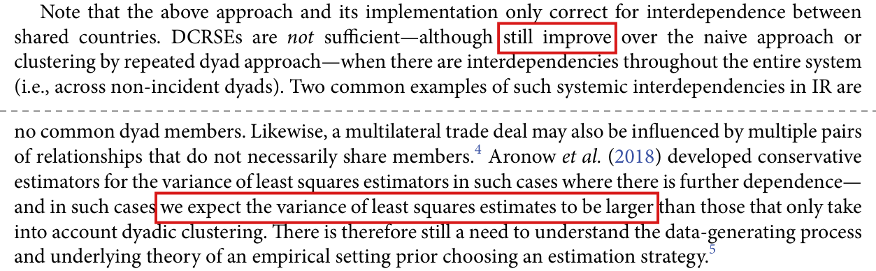
Two groups of lines from one paragraph, separated by a dashed grey rule. In the first group a red box surrounds 'still improve' in the sentence 'DCRSEs are not sufficient, although still improve over the naive approach or clustering by repeated dyad approach, when there are interdependencies throughout the entire system'. In the second group a red box surrounds 'we expect the variance of least squares estimates to be larger', which follows 'Aronow et al. (2018) developed conservative estimators for the variance of least squares estimators in such cases where there is further dependence, and in such cases'.
Section 3, paragraph beginning “Note that the above approach”, p. 191 (PDF p. 6): its first four lines and its last six, with the four lines between them left out at the dashed rule. The marks are on “still improve” and on the expectation of a larger variance.
The six lines of the first paragraph of the Conclusion. A red box in the fifth line surrounds 'a lower bound', in the phrase 'thereby revealing a lower bound on the severity of the consequences of inadequate clustering practices in previous quantitative dyadic research'.
Conclusion, first paragraph, p. 196 (PDF p. 11). The mark is on “a lower bound”.
A line chart. The horizontal axis is the number of independent blocks of dyads, m, from 1 to 100 on a logarithmic scale. The vertical axis is the expected DCR variance estimate divided by the true variance, from 0.5 to 1.8. A horizontal line at 1 is labelled 'ratio 1: the estimate equals the true variance on average', and the region below it is shaded and labelled 'below 1: uncertainty is underestimated, the direction stated on p. 187'. A blue curve with circles, labelled 'Example 4: six dyads among four members', starts at 2/3 for m = 1, crosses 1 before m = 2, where it is 13/12, passes 17/12 at m = 10 and approaches a dashed line labelled 'limit 3/2'. An orange curve with squares, labelled 'Example 5: dyads (A,B), (A,C), (D,E), (D,F)', starts at 7/6 for m = 1, is 17/12 at m = 2 and approaches a dashed line labelled 'limit 5/3'. The title reads 'Negative dependence between non-incident dyads: the DCR variance estimate settles above the true variance in both examples'.
Expected value of the DCR variance estimator, without a small-sample correction, divided by the true variance of the estimated intercept, for mm independent blocks of Example 4 (circles, curve 3/2−5/(6m)3/2-5/(6m)) and of Example 5 (squares, curve (10m−3)/(6m)(10m-3)/(6m)). The markers are the values computed exactly for m=1,2,10m=1,2,10 and for m=1,2m=1,2, and the dashed lines are the limits 3/23/2 and 5/35/3. A ratio above 1 means that the DCR variance estimate is too large on average; both limits contradict the unconditional underestimation claim on p. 187.
My comment and the history of this entry

Agreed. The sign condition was implicit to our understanding of the natural of these problems typically, though we did not state it explicitly.

  1. Classification before my review (the classification when the audit was first completed, before I reviewed it): Moderate error.
  2. I commented.
  3. Independent evaluation. No change was needed. The independent check found that the usual setting of these problems does not by itself ensure the sign condition, so the entry remains a Moderate error. My report that the condition was implicit is my own account and could not be verified independently.

In the Stata command, the branch that should fit the comparison model with a robust variance when rse is requested tests crse a second time and can never run; for seven KEVs in three models of Kinne (2018) and Weisiger (2016), the comparison standard error, its pp-value and the denominator of the SER then come from the default variance of the estimation command and not from the robust variance of the original study, and line 321 should test rse.

Section 4.1, p. 193 (PDF p. 8), definition of the standard error ratio. Stata package dcr (commit 734ee6a) and its identical copy in the replication files: dcr.ado, lines 310–334, and the help entry for rse; calls on lines 352, 381 and 1199 of the replication script 1_reanalysis_stata.do. The code is not printed in the article.

As printed

P. 193: “We compute a standard error ratio (SER) for all KEVs, which is the DCRSE divided by the standard error produced using the original variance estimation strategy.13{}^{13}”

Stata help: “rse specifies that a robust standard error (RSE) should be computed in addition to a DCRSE, e.g., for the purpose of calculating the ratio of DCRSE to RSE. This RSE is only output to the Excel spreadsheet created by xlsxpath.”

dcr.ado, line 310 and lines 320–334. Lines 311–319 hold the three clustered fits of the first branch, omitted here.

if ("`crse'"!="") {

}

else if ("`crse'"!="") {

if "`syntax'" == "vce" {

qui `prefix' `command_line' if `touse' `weight', `options' vce(robust)

}

if "`syntax'" == "clusterOnly" {

qui `prefix' `command_line' if `touse' `weight', `options'

}

if "`syntax'" == "robustCluster" {

qui `prefix' `command_line' if `touse' `weight', `options' robust

}

}

else {

qui `prefix' `command_line' if `touse' `weight', `options'

}

The problem

Beside the DCRSE, the command exports a comparison standard error from a second fit of the model, and the ratio of the two is the SER of the reanalysis. Three branches choose the second fit. The first runs when crse is given and clusters on the named variable. The second is meant to run when rse is given and to use the robust variance of the estimation command. Its condition repeats that of the first. The branch is reached only when crse is empty and entered only when crse is not empty, which cannot happen. No other line tests rse. A call with rse and without crse then falls to the third branch, which fits the model without adding a variance option. For the reanalysis calls, the comparison standard error, its pp-value and the SER are then computed from the default variance of the estimation command. The reanalysis has nine such calls. Six are stcrreg models, whose default variance is already robust, and for them the defect need not change anything. Three are models whose default variance is not robust and whose original fit asked for a robust one: the logit model of Kinne (2018), Figure 8, Model 1, and the stcox models of Weisiger (2016), Table 3, Model 1 and Table 4, Model 1. Their seven KEVs, two of the six of Kinne and five of the 28 of Weisiger, are compared with a standard error that does not come from the original variance estimation strategy.

Evidence an exact counterexample

I checked the code and computed two exact examples. In dcr.ado the word rse occurs only on line 16, where the option is declared, and on line 36, where it is removed from the options passed to the estimation command. Lines 310 and 321 carry the same test.

In the example, y=(0,0,1,3)y=(0,0,1,3) is regressed on an intercept and x=(−1,0,0,1)x=(-1,0,0,1), the four dyads share no member, and the command is called with rse and dofundo(reglike). Then β^=(1, 3/2)\widehat\beta=(1,\,3/2), the residuals are (1/2,−1,0,1/2)(1/2,-1,0,1/2), and the three variance matrices are diagonal.

The exact example: the slope, as the command exports it and as rse requests it.
QuantityAs exportedWith the robust comparison
Comparison variance of the slope3/83/8 (default)1/41/4 (robust)
DCR variance of the slope1/81/81/81/8
Squared SER1/31/31/21/2
Squared zz statistic of the comparison fit6699

A second exact example is a logit model on the fifteen dyads among six members. Its slope has default variance 47/8447/84, robust variance 2045/54882045/5488 and DCR variance 195/392195/392. The squared SER is 585/658<1585/658<1 as exported and 546/409>1546/409>1 with the robust comparison. In this example the defect moves the ratio from one side of one to the other.

I computed both examples from the formulas of the command and of the estimation commands; I did not run Stata. The seven KEVs are listed below with the values that the command exported. They are not corrected values. I did not fit the three models again.

The seven KEVs whose comparison standard error comes from the default variance: saved values of the primary reanalysis.
ModelKEVComparison SEDCRSESER
Kinne (2018), Figure 8, Model 1l_DCA2paths0.06820.09601.407
Kinne (2018), Figure 8, Model 1l_DCAdegree0.06640.15052.267
Weisiger (2016), Table 3, Model 1lndeadpop0.09060.71357.872
Weisiger (2016), Table 3, Model 1pcturnsum0.72621.48582.046
Weisiger (2016), Table 4, Model 1lndeadpop0.09130.68537.505
Weisiger (2016), Table 4, Model 1pcncsum0.97491.14801.178
Weisiger (2016), Table 4, Model 1pcnewcsum1.10521.59731.445
What survives

The definition of the SER on p. 193 is correct. The DCR variance is computed before this block and is unchanged by this repair, as are the coefficients, the DCRSEs and the pp-values based on them. The R package, the calls with crse and the calls with neither option are not affected. The comparison standard errors, their pp-values and the SERs of the seven KEVs need to be recomputed; I have not measured their numerical changes. They enter the rows Kinne (2018) and Weisiger (2016) of Supplementary Table A.2, the 2016, 2018, Security and All rows of Table 5, Figures 1–3 and, through the small-sample scripts, Supplementary Table A.5. Under the inverse study frequency weighting the seven KEVs carry (2/6+5/28)/22(2/6+5/28)/22, about 2%, of the total weight; without an upper bound on their corrected ratios, this gives no upper bound on the corrected mean SER. No rounded figure of the article, the 1.74, the 0.22 and the 67% among them, is shown to change. The DCRSEs of the Weisiger models are the subject of P032-N004.

Corrected

dcr.ado, line 321, with the three fits on lines 322–330 kept:

else if ("`rse'"!="") {

After this change, I would refit the comparison models of Kinne (2018), Figure 8, Model 1 and of Weisiger (2016), Table 3, Model 1 and Table 4, Model 1 in the primary and in the small-sample scripts, and regenerate the comparison standard errors, the pp-values, the SERs and the tables and figures that use them. I give no corrected values, since they require these fits.

Crop of six lines of page 193, from 'To quantify the impact of neglecting dyadic clustering'. Two red boxes mark the words 'the standard error produced using the original variance estimation strategy', which run over two lines and end with the footnote mark 13.
Section 4.1, p. 193 (PDF p. 8). The marked words define the denominator of the SER. For seven KEVs the command exports a standard error from the default variance of the estimation command, while the original studies used a robust one. The definition is correct as printed.

On a subset or reordered data frame, or with member labels that contain underscores, the R routines dcr() and dcr_sandwich() can return a wrong covariance matrix without a warning, because they read row names as row positions and join the two member labels of a dyad with an underscore.

Section 5 (Conclusion), p. 196 (PDF p. 11), sentence beginning “These open-source packages”; R package dcr, file R/dyad_funcs.R, lines 34–35 and 111–112, and file R/helper_funcs.R, line 38

As printed

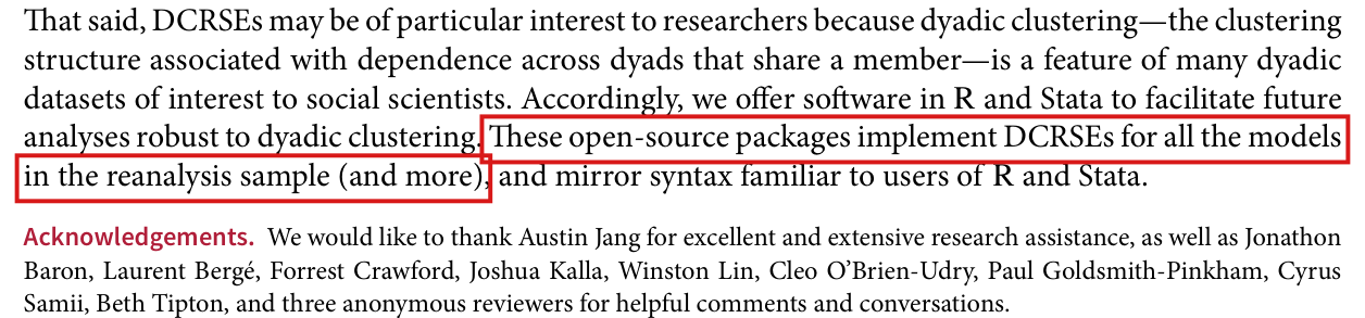
p. 196. These open-source packages implement DCRSEs for all the models in the reanalysis sample (and more), and mirror syntax familiar to users of R and Stata.

R/dyad_funcs.R, lines 34–35, in dcr(); repeated at lines 111–112, in dcr_sandwich().

touse_obs <- as.integer(rownames(model.frame(model)))

touse_data <- data[touse_obs,]

R/helper_funcs.R, line 38, in create_dyadid().

dyad_id <- unlist(lapply(sorteddyads, function(x) as.factor(paste0(x, collapse = "_"))), use.names = F)

The problem

The R package is the released implementation of the estimator on p. 191,

V^r=∑i=1NV^c,i−V^D−(N−2)V^0.\widehat V_r=\sum_{i=1}^{N}\widehat V_{c,i}-\widehat V_D-(N-2)\widehat V_0 .

Both routines convert the row names of the fitted model frame to integers and use them as row positions in the data. Row names label rows; subsetting or reordering a data frame can preserve names that no longer equal row positions. This can make dcr() build its list of dyad members from the wrong rows, so that NN and the sum over members can be wrong; dcr_sandwich() can also attach cluster labels to the wrong observations. Separately, create_dyadid() labels a dyad by sorting its two member labels and joining them with an underscore. The pairs (A_B, C) and (A, B_C) both receive the label A_B_C. Two dyads that share no member are then treated as one repeated dyad in V^D\widehat V_D. In each case the routine returns a covariance matrix and gives no warning. The inputs are ordinary. The replication script itself passes a subset of the data for models 1 and 2 of Pratt (2018), where the result happens to be unaffected, and nothing in the documentation of the package excludes underscores in member labels.

Evidence an exact counterexample

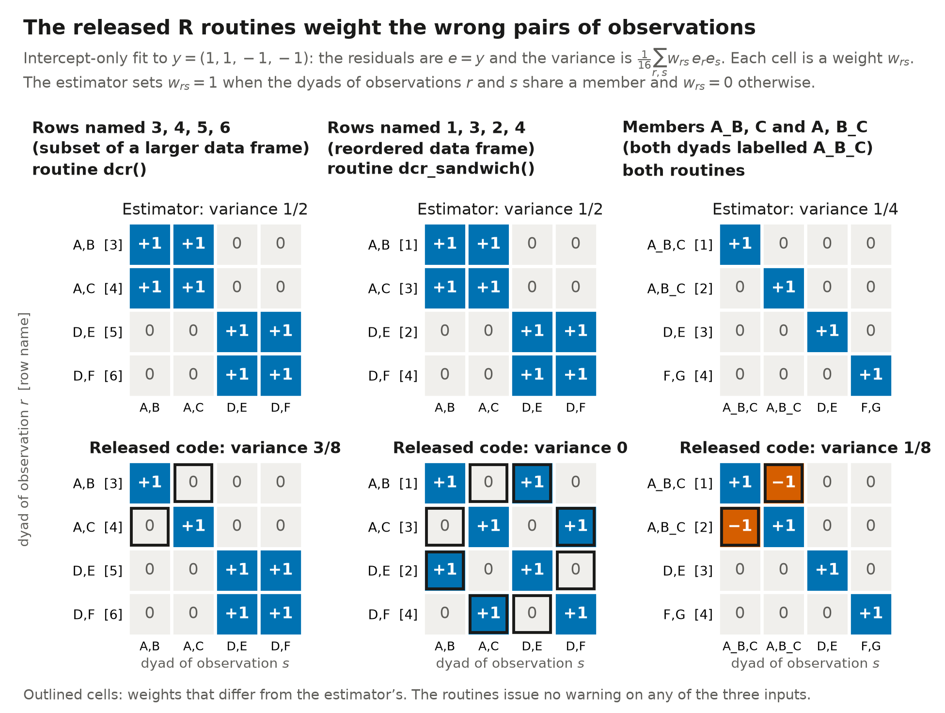
The evidence is three exact examples, computed in rational arithmetic and reproduced by running the unmodified package. Each has four observations, responses y=(1,1,−1,−1)y=(1,1,-1,-1) and a least-squares fit with an intercept only. The fitted intercept is 00, the residuals equal yy, and every variance below is a sum of products of residuals divided by 1616.

Variance of the intercept estimate in three exact examples.
DyadsRow namesRoutineMembers countedReturnedCorrect
A–B, A–C, D–E, D–F3, 4, 5, 6dcr()3 of 63/83/81/21/2
A–B, A–C, D–E, D–F1, 3, 2, 4dcr_sandwich()6 of 6001/21/2
A_B–C, A–B_C, D–E, F–G1, 2, 3, 4both8 of 81/81/81/41/4

Since the dyads are distinct in the first two examples, V^D=V^0=4/16=1/4\widehat V_D=\widehat V_0=4/16=1/4. The clusters of members A and D each give (22+1+1)/16=3/8(2^2+1+1)/16=3/8, and the other four members give 1/41/4 each. By the decomposition, I have

V^r=74−14−4⋅14=12.\widehat V_r=\frac{7}{4}-\frac{1}{4}-4\cdot\frac{1}{4}=\frac{1}{2}.

With row names 3 to 6, dcr() reads rows 3 and 4 of the four-row frame and two rows that do not exist. It finds the members D, E and F only, and returns

78−14−(3−2)⋅14=38.\frac{7}{8}-\frac{1}{4}-(3-2)\cdot\frac{1}{4}=\frac{3}{8}.

With row names 1, 3, 2, 4, dcr_sandwich() assigns member A to observations 1 and 3 and member D to observations 2 and 4. The residuals in each of these clusters sum to zero, so the clusters of A and D give 2/16=1/82/16=1/8 each, and the routine returns

2⋅18+4⋅14−14−4⋅14=0.2\cdot\frac{1}{8}+4\cdot\frac{1}{4}-\frac{1}{4}-4\cdot\frac{1}{4}=0.

In the third example the eight members are distinct. Then no two observations share a member, and I find V^r=V^0=1/4\widehat V_r=\widehat V_0=1/4. Since the first two dyads are both labelled A_B_C, the routines compute V^D={(1+1)2+1+1}/16=3/8\widehat V_D=\{(1+1)^2+1+1\}/16=3/8 in place of 1/41/4 and return

8⋅14−38−6⋅14=18.8\cdot\frac{1}{4}-\frac{3}{8}-6\cdot\frac{1}{4}=\frac{1}{8}.

Row names 101101 to 104104, or names that are not numbers, make both routines stop with an error. With the two changes given below, both routines return 1/21/2, 1/21/2 and 1/41/4 on these inputs.

What survives

This finding does not concern the estimator, its decomposition on p. 191, the Stata command or the simulations. No number reported in the paper is shown to change. For fits 1 to 5 of Pratt (2018), the covariance matrix without the optional small-sample and positive-semidefinite adjustments agrees with an independent calculation to within 10−810^{-8}, all 1616 members (fits 1 and 2) and all 2525 members (fits 3 to 5) are counted, and no distinct dyads share a label. The three Arel-Bundock (2017) fits and the sixth Pratt fit could not be checked.

Corrected

R/dyad_funcs.R, in dcr() and in dcr_sandwich().

touse_obs <- match(rownames(model.frame(model)), rownames(data))

stopifnot(!anyNA(touse_obs), !anyDuplicated(touse_obs))

touse_data <- data[touse_obs,]

R/helper_funcs.R, in create_dyadid(), in place of paste0(x, collapse = "_").

paste0(nchar(enc2utf8(x), type = "bytes"), ":", enc2utf8(x), collapse = "")

The first change matches each fitted row to the row of the data with the same name and stops if a fitted row has no match or two fitted rows match the same data row. The matching must also be used to align every clustering vector to the model’s observation order, preserving each covariance routine’s handling of omitted rows. Where row names cannot recover this correspondence, the routines should require an explicit observation identifier. The second change puts both labels in UTF-8 and writes each label’s byte length before it, so that (A_B, C) becomes 3:A_B1:C and (A, B_C) becomes 1:A3:B_C; grouping on the two sorted columns jointly serves equally well. The same change applies to the copies of create_dyadid() in the two R replication scripts. Neither change alters the estimator.

Crop of the last five lines of the Conclusion and the start of the Acknowledgements. A red outline marks the words: These open-source packages implement DCRSEs for all the models in the reanalysis sample (and more).
p. 196 (PDF p. 11), last paragraph of the Conclusion. The marked clause presents the R and Stata packages as implementations of DCRSEs for the models of the reanalysis; the finding concerns the R package.
Six four-by-four grids in two rows and three columns. Each cell holds a weight, plus one, zero or minus one, for a pair of observations. Top row, the estimator: in the first two columns, two blocks of plus ones for the dyads that share member A and the dyads that share member D, variance one half; in the third column, plus ones on the diagonal only, variance one quarter. Bottom row, the released code: in the first column the two off-diagonal weights for the dyads A,B and A,C are zero, variance three eighths; in the second column the plus ones link observations 1 and 3 and observations 2 and 4, variance zero; in the third column the off-diagonal weights between the first two dyads, whose labels collide, are minus one, variance one eighth. The cells that differ from the estimator are outlined.
Three exact examples with four observations, responses y=(1,1,−1,−1)y=(1,1,-1,-1) and an intercept-only fit. The top row shows the weights on pairs of observations that the estimator defines, and the bottom row the weights that the released routines use on that input. The routines return the variances 3/83/8, 00 and 1/81/8 where the estimator gives 1/21/2, 1/21/2 and 1/41/4.

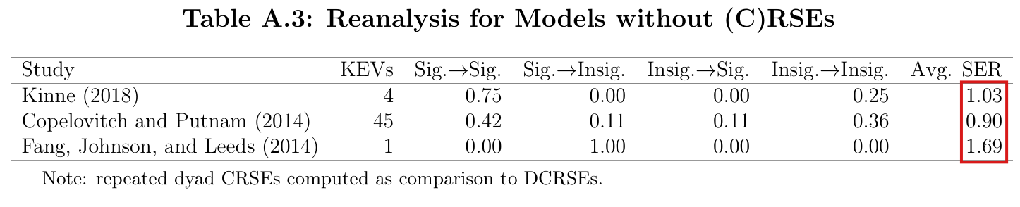
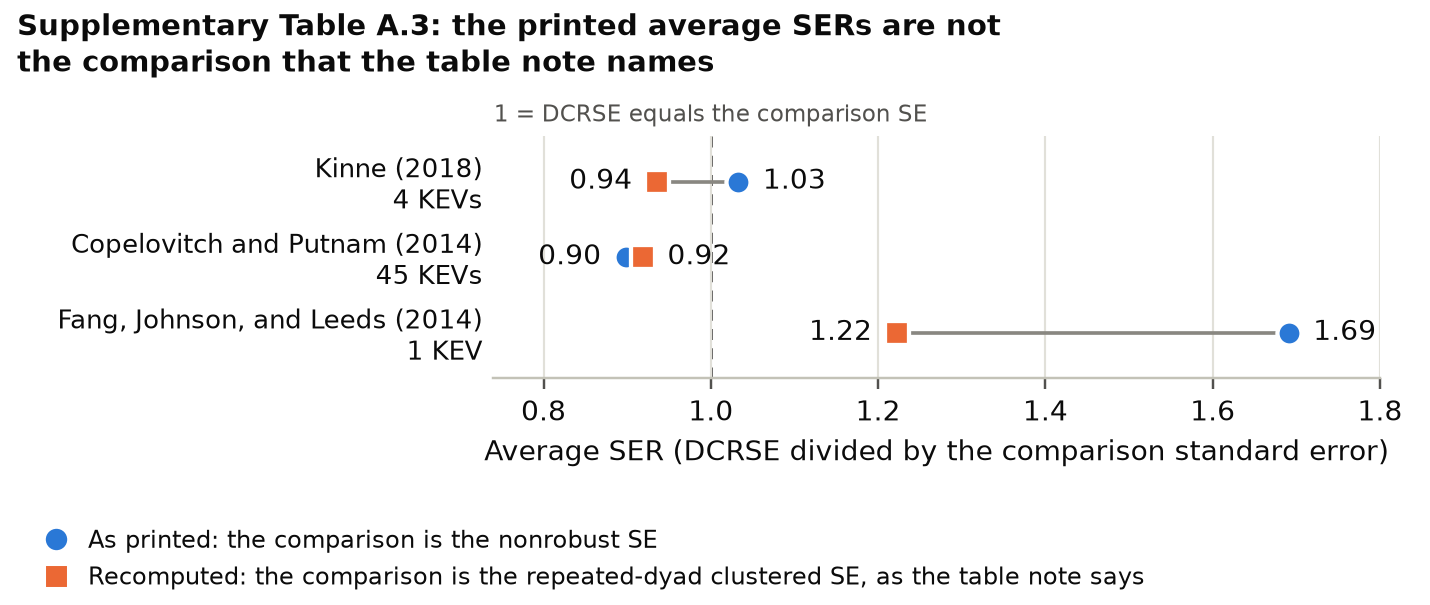
The three average SERs of Supplementary Table A.3 divide the DCRSE by the nonrobust standard error of the primary analysis and not by the repeated-dyad clustered standard error that the table note and footnote 9 name; with the stated comparison they are 0.94, 0.92 and 1.22 in place of 1.03, 0.90 and 1.69.

Supplementary Table A.3, column Avg. SER, p. A4 (PDF p. 4 of the supplement), cited in footnote 9, p. 192 (PDF p. 7). Replication script: 3_reanalysis_merge.R, block “CRSE REDO”, lines 707–739. The code is not printed in the article.

As printed

Supplementary Table A.3, p. A4:

Table A.3: Reanalysis for Models without (C)RSEs
StudyKEVsSig.→\toSig.Sig.→\toInsig.Insig.→\toSig.Insig.→\toInsig.Avg. SER
Kinne (2018)40.750.000.000.251.03
Copelovitch and Putnam (2014)450.420.110.110.360.90
Fang, Johnson, and Leeds (2014)10.001.000.000.001.69

“Note: repeated dyad CRSEs computed as comparison to DCRSEs.”

Footnote 9, p. 192: “See Supplementary Table A.3 for a summary of the results of DCR estimation for these models when repeated dyad cluster robust standard errors are added in.”

3_reanalysis_merge.R, line 710, the first of 24 calls of this form on lines 710–738:

analysis_extract_stata(here("results", "reanalysis_stata", "copelovitch2014/t1m2.xlsx"), kev = c("uncertainty")),

The problem

Twenty-four models in three studies used neither robust nor clustered standard errors. The Stata script runs the DCR command on each of them twice. The first run uses the comparison standard error of the original study, which is the nonrobust one, and the second uses a standard error clustered on repeated dyads. The script writes the two sets of results to two folders. The block of the merge script that builds Table A.3 reads the first folder for all 24 models. The column Avg. SER then repeats ratios of the primary analysis. The entries for Copelovitch and Putnam and for Fang, Johnson, and Leeds are rounded versions of those in their rows in Supplementary Table A.2, 0.898 and 1.691. The table does not report the comparison that its note and footnote 9 describe. The difference changes how the table is read. For Kinne (2018) the average ratio is below one and not above it. For Fang, Johnson, and Leeds (2014) the DCRSE is about 22% larger than the repeated-dyad clustered standard error, in place of the roughly 69% implied by the printed ratio.

Evidence a recalculation from the source

The evidence is a recalculation from the saved result files of the replication package. No model was fitted again. I applied the rules of the merge script to the 50 KEVs that the block selects, once in the 24 files that it reads and once in the 24 files that the Stata script writes for the clustered comparison. The rules round each ratio to three decimals, average the rounded ratios, round the mean to three decimals and display it to two decimals. The coefficients and DCRSEs agree up to numerical rounding; the comparison standard errors and their p-values change.

Average SER of Supplementary Table A.3 under the two comparison standard errors. “Files read” are the result files with the nonrobust comparison, which the block reads; “clustered files” are those written for the repeated-dyad clustered comparison. Means are of ratios rounded to three decimals.
StudyKEVsPrintedFiles readClustered files
Kinne (2018)41.031033/1000=1.0331033/1000=1.0333741/4000=0.935253741/4000=0.93525
Copelovitch and Putnam (2014)450.9040417/45000≈0.8981640417/45000\approx0.8981641351/45000≈0.9189141351/45000\approx0.91891
Fang, Johnson, and Leeds (2014)11.691691/1000=1.6911691/1000=1.691611/500=1.222611/500=1.222

The files that the block reads reproduce the printed column exactly. For each of the 50 KEVs the significance category at the 5% level is the same in both sets of files, so the four proportions of each row are unchanged. As an instance, the one KEV of Fang, Johnson, and Leeds has DCRSE 0.23080.2308, nonrobust standard error 0.13650.1365 and repeated-dyad clustered standard error 0.18890.1889, to four decimals; the two ratios round to 1.6911.691 and 1.2221.222.

What survives

The numbers of KEVs and the four significance proportions of Table A.3 are unchanged, and the table note and footnote 9 stand once the column is corrected. Table 5, with the average SER of 1.74 and the significance-loss proportion of 0.22, Figures 1–3 and Supplementary Tables A.1, A.2 and A.4 are built from other objects of the script and do not change under this correction. The merge script for the small-sample correction makes the same choice of folder in a block whose table is not printed.

Corrected

Supplementary Table A.3, with the note unchanged:

Table A.3: Reanalysis for Models without (C)RSEs
StudyKEVsSig.→\toSig.Sig.→\toInsig.Insig.→\toSig.Insig.→\toInsig.Avg. SER
Kinne (2018)40.750.000.000.250.94
Copelovitch and Putnam (2014)450.420.110.110.360.92
Fang, Johnson, and Leeds (2014)10.001.000.000.001.22

3_reanalysis_merge.R, the 24 calls on lines 710–738, of which the first is

analysis_extract_stata(here("results", "reanalysis_stata_crse", "copelovitch2014/t1m2.xlsx"), kev = c("uncertainty")),

These are comparisons of saved estimates and not new fits.

The whole of Table A.3, Reanalysis for Models without (C)RSEs, with three rows: Kinne (2018), Copelovitch and Putnam (2014), and Fang, Johnson, and Leeds (2014). A red box marks the three entries of the last column, Avg. SER: 1.03, 0.90 and 1.69. Below the table is the note 'repeated dyad CRSEs computed as comparison to DCRSEs'.
Supplementary Table A.3, p. A4 (PDF p. 4 of the supplement). The marked column holds ratios of the DCRSE to the nonrobust standard error; the note below the table names the repeated-dyad clustered standard error as the comparison.
Crop of footnote 9 on page 192, between the last line of footnote 8 and footnote 10. Two red boxes mark the words 'repeated dyad cluster robust standard errors are added in', which run over two lines.
Footnote 9, p. 192 (PDF p. 7), which cites the table. The marked words state the comparison that the table is meant to report.
A dot chart with three rows and a horizontal axis for the average SER with tick marks from 0.8 to 1.8. Kinne (2018), 4 KEVs: a blue circle labeled 1.03, as printed, joined by a line to an orange square labeled 0.94, recomputed. Copelovitch and Putnam (2014), 45 KEVs: a blue circle labeled 0.90 and an orange square labeled 0.92. Fang, Johnson, and Leeds (2014), 1 KEV: a blue circle labeled 1.69 joined to an orange square labeled 1.22. A dashed vertical line at 1 is labeled DCRSE equals the comparison SE.
Means of three-decimal SERs for each row of Supplementary Table A.3, using the nonrobust comparison (circles) and the repeated-dyad clustered comparison (squares); labels are rounded to two decimals. The dashed line marks a ratio of one. For Kinne (2018) the recomputed ratio is below one; for Fang, Johnson, and Leeds (2014) it rounds to 1.22 in place of 1.69.

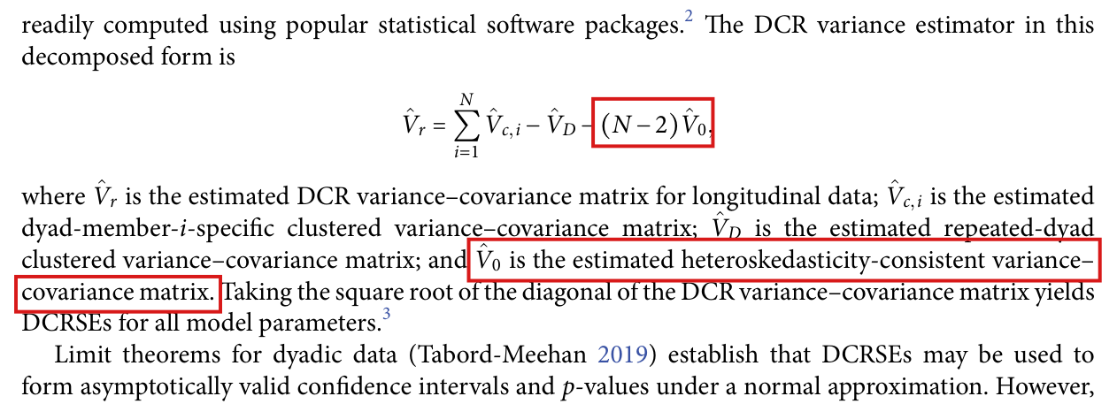
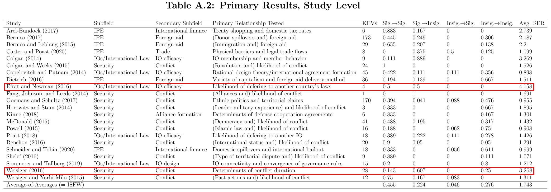
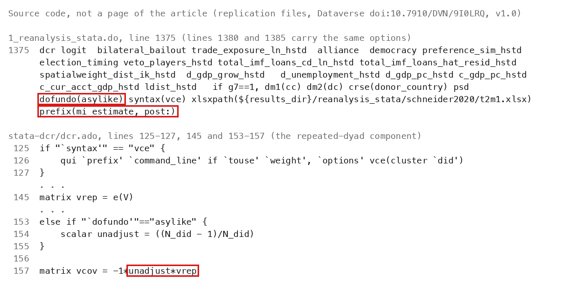
For the 13 survival models behind the Efrat and Newman (2016) and Weisiger (2016) rows of Supplementary Table A.2, the Stata command takes V^0\widehat V_0 from a fit with vce(robust), whose variance on data declared with stset and an id() variable is clustered on that variable and is not the observation-level matrix that the decomposition requires; the piece should be clustered on an observation index and the 13 models fitted again.

Display for V^r\widehat V_r and definition of V^0\widehat V_0, p. 191 (PDF p. 6); Supplementary Table A.2, rows Efrat and Newman (2016) and Weisiger (2016), p. A3 (PDF p. 3 of the supplement). Replication files: dcr.ado, lines 163–190, and 1_reanalysis_stata.do, lines 319–334 and 347–418. The code is not printed in the article.

See also under Formal statements (Lean): P032-T3, P032-T4, P032-T11

As printed

P. 191:

V^r=∑i=1NV^c,i−V^D−(N−2)V^0,\widehat V_r=\sum_{i=1}^{N}\widehat V_{c,i}-\widehat V_D-(N-2)\widehat V_0,

where … V^0\widehat V_0 is the estimated heteroskedasticity-consistent variance–covariance matrix.

dcr.ado, lines 164, 178 and 190, in the block headed “Calculate heteroskedasticity robust vcov”:

qui `prefix' `command_line' if `touse' `weight', `options' vce(robust)

matrix vhet = e(V)

matrix vcov = vcov - ((N_ud - 2)*unadjust*vhet)

1_reanalysis_stata.do, line 319 (Efrat and Newman) and line 347 (Weisiger). Lines 355, 368, 376, 384 and 397 declare the same id as line 347, and line 408 declares id(idvar).

stset T1, failure(acceptance==1) id(dyad)

stset warday, id(warnum) f(endday)

Supplementary Table A.2, p. A3, columns KEVs, Sig.→\toSig., Sig.→\toInsig., Insig.→\toSig., Insig.→\toInsig., Avg. SER. Efrat and Newman (2016): 4, 0.5, 0.5, 0, 0, 4.158. Weisiger (2016): 28, 0.143, 0.607, 0, 0.25, 3.268.

The problem

The decomposition is an identity when all of its pieces are sums over the contributions of the same observations, where an observation is one row of the data. In V^c,i\widehat V_{c,i} all observations whose dyad contains member ii form one cluster and each other observation is its own cluster, and in V^0\widehat V_0 every observation is its own cluster. The Stata command builds the member-specific pieces in this way. It obtains V^0\widehat V_0 by fitting the model again with vce(robust), and it subtracts (N−2)(N-2) times the result. For stcox and stcrreg, on data declared with stset and an id() variable, the variance that Stata returns for vce(robust) is clustered on the id. The contributions of all observations with one id are summed before they are squared. The reanalysis declares such an id for the three stcox models of Efrat and Newman (2016) and for the ten models of Weisiger (2016), two stcox and eight stcrreg. These 13 models hold 32 KEVs. For them the command returns, before the eigenvalue step of footnote 3 and when every piece carries the same scaling,

∑i=1NV^c,i−V^D−(N−2)V^id=V^r+(N−2)(V^0−V^id),\sum_{i=1}^{N}\widehat V_{c,i}-\widehat V_D-(N-2)\widehat V_{\mathrm{id}}=\widehat V_r+(N-2)\bigl(\widehat V_0-\widehat V_{\mathrm{id}}\bigr),

where V^id\widehat V_{\mathrm{id}} is the variance matrix clustered on the id. The Weisiger calls set dofundo(asylike), which multiplies the piece by (n−1)/n(n-1)/n, with nn the number of observations, while the factor that Stata documents for a clustered variance is g/(g−1)g/(g-1), with gg the number of ids. The last term is then (N−2)(V^0−αV^id)(N-2)\bigl(\widehat V_0-\alpha\widehat V_{\mathrm{id}}\bigr) with α=((n−1)/n)(g/(g−1))\alpha=((n-1)/n)(g/(g-1)). The difference from V^r\widehat V_r has no fixed sign, and any difference between the two matrices is multiplied by N−2N-2. I did not fit the 13 models again, and I do not know the size or the sign of the difference in the two studies.

Evidence an exact counterexample

The evidence has three parts: a check of the code, the documentation of the two Stata commands, and an exact example.

In dcr.ado, lines 108–119 give all observations that contain a member the cluster value −99-99 and give every other observation its own row number. Lines 126 and 202 fit the repeated-dyad piece and the member-specific pieces with explicit cluster variables. Line 164 fits the piece called vhet with vce(robust), and line 190 subtracts (N−2)(N-2) times it.

The Stata Survival Analysis Reference Manual, Release 15 (StataCorp 2017), in the entry [ST] stcox, technical note under “Robust estimate of variance” (p. 17), says of vce(robust) on data with an id that “stcox knew to specify vce(cluster id)”, and it lets an explicit cluster variable override the id. The entry [ST] stcrreg, last paragraph of “Methods and formulas” (p. 24), states that the clustered version of the variance is used when a cluster variable is given “or an ID variable has been stset.” The description of noadjust in [ST] stcox (p. 4) gives the default multiplier as n/(n−1)n/(n-1) or g/(g−1)g/(g-1). I read these entries, and the current ones, which agree with them. I did not read Release 17, which the replication files name, and Stata was not run.

The example has six subjects, one for each dyad among four members, with ten observations, one covariate xx and no weights. Status 1 is the event of interest, and status 2 is a competing event, treated as censoring.

An exact survival example: ten observations, six ids, four dyad members.
RowIdDyadIntervalxxStatusScore at β^=0\widehat\beta=0
11{1,2}\{1,2\}(0,1](0,1]1112/32/3
22{3,4}\{3,4\}(0,1](0,1]−1-11−2/3-2/3
33{1,3}\{1,3\}(0,1](0,1]110−1/3-1/3
43{1,3}\{1,3\}(1,2](1,2]3313/23/2
54{2,4}\{2,4\}(0,1](0,1]−1-101/31/3
64{2,4}\{2,4\}(1,2](1,2]−3-31−3/2-3/2
75{1,4}\{1,4\}(0,1](0,1]110−1/3-1/3
85{1,4}\{1,4\}(1,3](1,3]112−1/2-1/2
96{2,3}\{2,3\}(0,1](0,1]−1-101/31/3
106{2,3}\{2,3\}(1,3](1,3]−1-121/21/2

With Breslow ties the Cox partial likelihood is maximized at β^=0\widehat\beta=0, the information is 1212, and the scores of the ten observations are those of the last column. Multiplying the sums of squared scores by 1/1441/144, I obtain the pieces below.

The pieces of the decomposition in the example (N=4N=4), and what the decomposition returns.
QuantityValue
V^0\widehat V_0, every observation its own cluster19/43219/432
V^id\widehat V_{\mathrm{id}}, clustered on the id (equal to V^D\widehat V_D here)15/43215/432
∑iV^c,i\sum_i\widehat V_{c,i}68/43268/432
Decomposition as printed: ∑iV^c,i−V^D−2V^0\sum_i\widehat V_{c,i}-\widehat V_D-2\widehat V_015/432=5/14415/432=5/144
With V^id\widehat V_{\mathrm{id}} in place of V^0\widehat V_023/43223/432
With αV^id\alpha\widehat V_{\mathrm{id}} in place of V^0\widehat V_0, α=(9/10)(6/5)=27/25\alpha=(9/10)(6/5)=27/25103/2160103/2160

The printed decomposition returns 5/1445/144, which is also the sum of the products of all pairs of observations that share a member. With the variance matrix clustered on the id, it returns a variance 23/1523/15 times as large, and with the factor of the Weisiger calls a variance 103/75103/75 times as large. All three values are positive, so the eigenvalue step changes none of them.

The identity in the corrected statement holds by counting. The product zrzs⊤z_rz_s^\top of two observations enters ∑iV^c,i\sum_i\widehat V_{c,i} once for each member ii for which the two observations lie in one cluster. If r=sr=s, this happens NN times, and subtracting V^D\widehat V_D and (N−2)V^0(N-2)\widehat V_0 leaves N−1−(N−2)=1N-1-(N-2)=1. If r≠sr\ne s and the two observations have the same dyad, it happens twice, and subtracting V^D\widehat V_D leaves 11. If the dyads differ and share one member, it happens once and nothing is subtracted. If the dyads share no member, the product does not appear.

What survives

The printed decomposition is correct as an identity, and the 20 studies that are not fitted with these survival commands are not touched by this point. What changes is the standing of the two rows of Supplementary Table A.2. They are not shown to be DCRSEs as p. 191 defines them. The two rows enter the 2016, IOs/International Law, Security and All rows of Table 5, the upper end of the range “0.90 to 4.16” on p. 196, Figures 1–3 and, through the small-sample scripts, Supplementary Table A.5. No corrected value has been computed, and none of these numbers is shown to change. The following averages show how much rests on the two rows and are not corrections. The mean of the Avg. SER column of Table A.2 over the other 20 studies is 1.546, against 1.743 over all 22. The mean for IOs/International Law without Efrat and Newman is 1.701, and the mean for Security without Weisiger is 1.338.

Corrected

The decomposition, with the conditions under which it is an identity. Let each observation rr of the estimation sample have an unordered dyad drd_r of two distinct members, let NN be the number of distinct members, and let zrz_r be the contribution of observation rr to the estimate, that is, its score contribution multiplied by the common bread matrix. Let all pieces come from one fit on one sample, without finite-sample factors:

V^0=∑rzrzr⊤,V^D=∑r,s: dr=dszrzs⊤,V^c,i=∑r,s: i∈dr∩dszrzs⊤+∑r: i∉drzrzr⊤.\widehat V_0=\sum_r z_rz_r^\top,\qquad \widehat V_D=\sum_{r,s:\,d_r=d_s}z_rz_s^\top,\qquad \widehat V_{c,i}=\sum_{r,s:\,i\in d_r\cap d_s}z_rz_s^\top+\sum_{r:\,i\notin d_r}z_rz_r^\top .

Then

∑i=1NV^c,i−V^D−(N−2)V^0=∑r,s: dr∩ds≠∅zrzs⊤=V^r.\sum_{i=1}^{N}\widehat V_{c,i}-\widehat V_D-(N-2)\widehat V_0=\sum_{r,s:\,d_r\cap d_s\ne\varnothing}z_rz_s^\top=\widehat V_r .

In particular, V^0\widehat V_0 is clustered on single observations and not on the id of the survival-time data.

In dcr.ado, for a command run on data with an stset id, the piece vhet is fitted with an explicit cluster variable that takes a different value on every observation of the estimation sample, in place of vce(robust). The stset id is kept, since stcrreg uses it for its censoring weights. Every piece is fitted with noadjust and dofundo(none), or the factor that the command applied to a piece is removed with the number of clusters which that fit reports, so that all pieces carry the same scaling. This describes the repair; it is not a patch that has been run in Stata.

The rows Efrat and Newman (2016) and Weisiger (2016) of Supplementary Table A.2, and the entries of Table 5, Supplementary Table A.5 and Figures 1–3 that use them, are to be recomputed after the 13 models are fitted again. I give no corrected values.

Crop of the top of page 191: two lines of text, the displayed equation V hat r equals the sum over i from 1 to N of V hat c,i, minus V hat D, minus (N minus 2) V hat 0, and the paragraph that defines the four matrices. A red box marks the term (N minus 2) V hat 0 in the display. Two more red boxes mark the words 'V hat 0 is the estimated heteroskedasticity-consistent variance-covariance matrix', which run over two lines.
The decomposition on p. 191 (PDF p. 6). The marked term is the piece that the command takes from a fit with vce(robust); the marked words define it as the heteroskedasticity-consistent matrix, in which every observation is its own cluster. The display is correct as printed.
The whole of Table A.2, Primary Results, Study Level: 22 rows, one per study, with columns Study, Subfield, Secondary Subfield, Primary Relationship Tested, KEVs, four significance proportions and Avg. SER, and a last row Average-of-Averages. A red box marks the row Efrat and Newman (2016), IOs/International Law, 4 KEVs, Avg. SER 4.158. A second red box marks the row Weisiger (2016), Security, 28 KEVs, Avg. SER 3.268.
Supplementary Table A.2, p. A3 (PDF p. 3 of the supplement, shown upright). The marked rows are the two studies whose models are fitted with stcox and stcrreg. Their average SERs, 4.158 and 3.268, are the largest and the third largest of the table. The values are not shown to be wrong; they were not computed with the observation-level matrix.

Minor (11)

Real but inconsequential, for example a misprint that does not change a result.

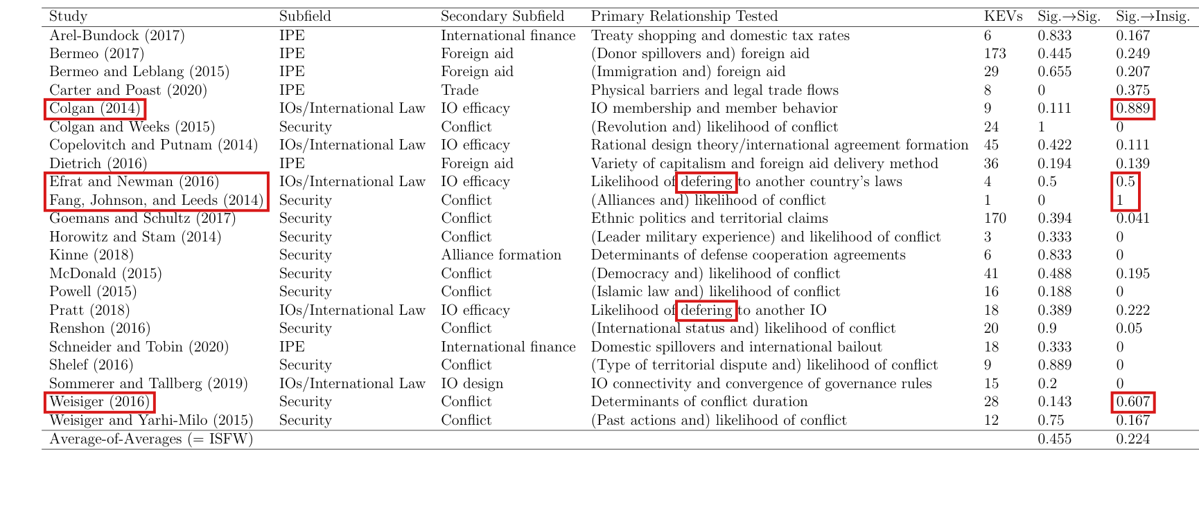
Four studies, not three, lose significance in half or more of their KEVs, and “deferring” is misspelled twice in Supplementary Table A.2.

Section 4.1, p. 196 (PDF p. 11), paragraph beginning “For individual studies”; Supplementary Table A.2, Supplementary Appendix p. A3 (PDF p. 3), entries for Efrat and Newman (2016) and Pratt (2018)

See also under Formal statements (Lean): P032-T10

As printed

p. 196. Three studies see half or more of their KEVs become insignificant at the 5% level upon reanalysis.

Table A.2, column “Primary Relationship Tested”. Efrat and Newman (2016): Likelihood of defering to another country’s laws. Pratt (2018): Likelihood of defering to another IO.

The problem

Supplementary Table A.2 lists four studies in which the share of KEVs that go from significant to insignificant is one half or more: Colgan (2014) with 8/98/9, Efrat and Newman (2016) with 2/42/4, Fang, Johnson, and Leeds (2014) with 1/11/1 and Weisiger (2016) with 17/2817/28. Three of them are strictly above one half.

Evidence a historical Lean attribution (Generated status: clause support not certified in this release)

The evidence is a recount from the column Sig.→\toInsig. of Table A.2, where every other study is at 0.3750.375 or below. The four counts agree with the saved model outputs in the replication files. The spelling is a check of the page.

What survives

The numerical entries of Table A.2 and every aggregate are unchanged. The neighbouring counts in the paragraph, 1818 of 2222 studies with an average SER above one and 77 of 2222 that lose no significance, agree with the table.

Corrected

p. 196. Four studies see half or more of their KEVs become insignificant at the 5% level upon reanalysis.

Table A.2. Efrat and Newman (2016): Likelihood of deferring to another country’s laws. Pratt (2018): Likelihood of deferring to another IO.

Alternatively, the sentence on p. 196 keeps “Three” and reads “more than half” in place of “half or more”.

Crop of the paragraph that begins For individual studies, showing six complete lines and part of the next. A red outline marks the sentence: Three studies see half or more of their KEVs become insignificant at the 5 percent level upon reanalysis.
p. 196 (PDF p. 11), Section 4.1, paragraph beginning “For individual studies”. The marked sentence gives the count as three.
Crop of Table A.2 with one row per study. Red outlines mark the study names Colgan (2014), Efrat and Newman (2016), Fang, Johnson, and Leeds (2014) and Weisiger (2016), and their entries 0.889, 0.5, 1 and 0.607 in the column Sig. to Insig. Two further red outlines mark the word defering in the rows for Efrat and Newman (2016) and Pratt (2018).
Supplementary Appendix, p. A3 (PDF p. 3), Table A.2, columns “Study” to “Sig.→\toInsig.”. The four studies with an entry of 0.50.5 or more are marked, with their entries 0.8890.889, 0.50.5, 11 and 0.6070.607, and so is the word “defering” in two rows.

The option of the R and Stata packages that is documented to force the variance matrix to be positive semidefinite replaces negative eigenvalues by zero only when a diagonal entry of the matrix is negative, and it can return an indefinite matrix; the eigenvalue step should run whenever the option is set.

Footnote 3, p. 191 (PDF p. 6), and the software option that it describes. R package dcr (commit 06a80ad): R/dyad_funcs.R, lines 70 and 155, and the help entry for posdef. Stata package dcr (commit 734ee6a): dcr.ado, lines 246–282, and the help entry for psd. The code is not printed in the article.

See also under Formal statements (Lean): P032-T6, P032-T7

As printed

Footnote 3, p. 191:

To account for rare instances where negative parameter estimate variances arise due to non-positive semi-definite variance-covariance matrices, an “eigendecomposition of the estimated variance matrix … [that] converts any negative eigenvalue(s) to zero” and then reassembles the matrix to “force” positive semi-definiteness is performed, in line with suggestions from Cameron et al. (2011) and Cameron and Miller (2014).

R help, argument posdef of the functions dcr and dcr_sandwich: “A logical value indicating whether or not DCR variance-covariance matrix is forced to be positive semi-definite.”

R/dyad_funcs.R, lines 70 and 155:

if (sum(diag(V.hat) < 0) >= 1 & posdef == TRUE) {

Stata help: “psd forces the final variance-covariance matrix to be positive semi-definite.”

dcr.ado, line 268, inside the block that runs when psd is set. Lines 252–258 set the scalar Indnegvar to 1 only if a diagonal entry of the matrix is negative.

if (Indnegvar==1) {

The problem

A symmetric matrix whose diagonal entries are all positive can have a negative eigenvalue. Both packages run the eigenvalue step of footnote 3 only if some diagonal entry of the DCR variance matrix is negative. If the matrix is indefinite and its diagonal is positive, the step is skipped. The matrix that the option returns then assigns a negative variance to some linear combination of the coefficients. The help texts of both packages state without this restriction that the option forces the matrix to be positive semidefinite. Footnote 3 speaks of negative parameter variances, and the code agrees with it. The defect is in the guarantee of the software option.

Evidence an exact counterexample

The evidence is an exact counterexample, computed in rational arithmetic and reproduced by running both R functions.

I regress yy on an intercept and xx by least squares on the ten dyads among five members, taken in the order (1,2)(1,2), (1,3)(1,3), (2,3)(2,3), (1,4)(1,4), (2,4)(2,4), (3,4)(3,4), (1,5)(1,5), (2,5)(2,5), (3,5)(3,5), (4,5)(4,5), with

x=(3,0,2,1,−1,1,−3,−2,3,−2),y=(3,−2,−2,1,1,0,0,2,1,0).x=(3,0,2,1,-1,1,-3,-2,3,-2),\qquad y=(3,-2,-2,1,1,0,0,2,1,0).

Then

X⊤X=(102242),β^=(5/13, 1/13).X^\top X=\begin{pmatrix}10&2\\2&42\end{pmatrix},\qquad \widehat\beta=(5/13,\,1/13).

With N=5N=5, the decomposition of p. 191 gives, in the order (intercept, slope),

V^r=13655808(460765−79681−796817157).\widehat V_r=\frac{1}{3655808}\begin{pmatrix}460765&-79681\\-79681&7157\end{pmatrix}.

Since both diagonal entries are positive, neither package applies the eigenvalue step. The determinant of V^r\widehat V_r is −70529/308915776-70529/308915776, which implies that one eigenvalue is negative. For c=(1,6)c=(1,6), I have

c⊤V^r c=460765−12⋅79681+36⋅71573655808=−2377553655808<0,c^\top\widehat V_r\,c=\frac{460765-12\cdot 79681+36\cdot 7157}{3655808}=-\frac{237755}{3655808}<0,

and this is the estimated variance of the intercept plus six times the slope. Both functions of the R package, installed without modification, return this matrix when posdef = TRUE, with eigenvalues 0.129750.12975 and −0.00176-0.00176. For the Stata command, the same matrix follows from the source for the call dcr regress y x, dm1() dm2() dofundo(reglike) psd, up to the order of the coefficients. Stata was not run.

The corrected option returns a positive semidefinite matrix. In the notation of the corrected statement below, with qjq_j the columns of QQ, I have c⊤V+c=∑jmax⁡{λj,0} (qj⊤c)2≥0c^\top V_+c=\sum_j\max\{\lambda_j,0\}\,(q_j^\top c)^2\ge 0 for every vector cc.

What survives

Footnote 3 needs no change. The decomposition and the coefficient estimates are unaffected. The corrected option can change individual DCRSEs when it now leaves an indefinite matrix unchanged. A matrix that is already positive semidefinite is unchanged. Where the option already applies the eigenvalue step, the spectral formula is unchanged. The reanalysis scripts set this option. I did not examine whether any of the 174 models has an indefinite matrix with a positive diagonal, and no published number is shown to change.

Corrected

When the option is set, the packages eigendecompose the symmetric estimated variance matrix whatever the signs of its diagonal entries, replace each negative eigenvalue by zero and reassemble the matrix. For V=Qdiag⁡(λ1,…,λk)Q⊤V=Q\operatorname{diag}(\lambda_1,\dots,\lambda_k)Q^\top with QQ orthogonal, the option returns

V+=Qdiag⁡(max⁡{λ1,0},…,max⁡{λk,0})Q⊤,V_+=Q\operatorname{diag}\bigl(\max\{\lambda_1,0\},\dots,\max\{\lambda_k,0\}\bigr)Q^\top,

which is positive semidefinite.

R/dyad_funcs.R, lines 70 and 73, and likewise lines 155 and 158:

if (posdef == TRUE) {

V.hat <- decomp$vectors %*% diag(pos_eigens, nrow = length(pos_eigens)) %*% t(decomp$vectors)

The second argument of diag keeps the formula right for a model with one parameter, where R reads a single number as a dimension.

dcr.ado: the test on line 268 is removed, so that lines 269–281 run whenever psd is set.

In the example above, the corrected option returns approximately

(0.12609−0.02150−0.021500.00367).\begin{pmatrix}0.12609&-0.02150\\-0.02150&0.00367\end{pmatrix}.
Crop of footnote 3 on page 191, four lines of small type, below the last line of footnote 2. A red box marks the words 'negative parameter estimate variances' in the first line. A second red box marks the words 'force positive semi-definiteness', with force in quotation marks, in the third line.
Footnote 3, p. 191 (PDF p. 6). The first marked phrase is the case that the footnote addresses, a negative variance of a parameter estimate. The second is the result that the help text of the software promises whenever the option is set.

A selector in the merge script joins two parameter names into one string and so drops two KEVs of Bermeo and Leblang (2015): with them the sample has 693 KEVs, not 691, and that study has 31, not 29, while every printed ratio and proportion of Table 5 keeps its two-decimal value.

Section 4, p. 192 (PDF p. 7), sentence beginning “The final analytic sample”; Supplementary Table A.2, row Bermeo and Leblang (2015), p. A3 (PDF p. 3 of the supplement); column KEVs of Table 5, p. 193 (PDF p. 8). Replication files: code/3_reanalysis_merge.R, line 128, and the same line of code/dof_corrections/3_reanalysis_merge_dof.R. The code is not printed in the article.

As printed

P. 192: “The final analytic sample consisted of 691 KEVs across 174 models from 22 studies.”

3_reanalysis_merge.R, line 128:

analysis_extract_stata(here("results", "reanalysis_stata", "bermeo2015/t4m7.xlsx"), kev = c("listock_lag MigrationPolicy_lag", "policy_stock_lag")),

Supplementary Table A.2, p. A3, row Bermeo and Leblang (2015), columns KEVs, Sig.→\toSig., Sig.→\toInsig., Insig.→\toSig., Insig.→\toInsig., Avg. SER: 29, 0.655, 0.207, 0, 0.138, 2.2. Table 5, p. 193, column KEVs: 122 (2015), 270 (IPE), 691 (All).

The problem

The Stata script names three KEVs for Table 4, Model 7 of Bermeo and Leblang (2015). Its line 100 reads * Table 4, Model 7; KEV: listock_lag MigrationPolicy_lag policy_stock_lag. The saved results of that model have one row for each. The selector compares whole strings, and the string "listock_lag MigrationPolicy_lag" equals no parameter name. Only policy_stock_lag is kept, and two designated KEVs are left out of the sample. The merge script for the small-sample correction has the same line. The sentence on p. 192 counts correctly the sample that the script produced. The omission is in the sample.

Evidence a recalculation from the source

The evidence is a recalculation from the saved estimates of the replication files. I ran the authors' extraction function with the printed selector and with the three names separated. I find 29 rows for the study with the first and 31 with the second, in 11 models both times. The two restored rows have SER 2.218 (listock_lag) and 2.331 (MigrationPolicy_lag), and both are significant at the 5% level before and after. The counts follow by addition: 667+6+18=691667+6+18=691 becomes 669+6+18=693669+6+18=693, where 6 and 18 are the KEVs of the two studies analyzed in R, and the counts for 2015 and for IPE become 124 and 272. For the study, the script averages ratios rounded to three decimals, and 63.811/29≈2.20063.811/29\approx 2.200 becomes 68.360/31≈2.20568.360/31\approx 2.205. The overall average SER lies in [1.74304, 1.74314][1.74304,\,1.74314] before and in [1.74325, 1.74335][1.74325,\,1.74335] after, and it rounds to 1.743 both times. These are intervals because the means of the two R studies are known to three decimals.

What survives

The 174 models and the 22 studies are unchanged, as are all fitted coefficients and variances. Every printed SER and proportion of Table 5 keeps its two-decimal value, including 1.74, 0.22 and 0.05, and the overall average SER remains 1.743. What changes is the number of KEVs in Table 5 and in Supplementary Table A.5, the study row and three entries of the last row in Supplementary Table A.2, and Figures 1–3, which incorporate the two additional KEV estimates.

Corrected

P. 192: “The final analytic sample consisted of 693 KEVs across 174 models from 22 studies.”

Line 128 of both merge scripts, with the path unchanged:

kev = c("listock_lag", "MigrationPolicy_lag", "policy_stock_lag")),

Supplementary Table A.2, row Bermeo and Leblang (2015): 31, 0.677, 0.194, 0, 0.129, 2.205. Last row of the table: 0.456, 0.223, 0.046, 0.275, 1.743. Table 5 and Supplementary Table A.5, column KEVs: 124 (2015), 272 (IPE), 693 (All).

These values are conditional on the saved estimates. The tables and figures are to be regenerated from the corrected merge.

Crop of five lines of page 192. A red box marks the words '691 KEVs' in the sentence 'The final analytic sample consisted of 691 KEVs across 174 models from 22 studies', which carries the footnote mark 8.
Section 4, p. 192 (PDF p. 7). The marked count is that of the sample which the merge script produced; two KEVs that the Stata script designates are missing from it.
The title, the header and the first six rows of Table A.2, Primary Results, Study Level. In the third row, Bermeo and Leblang (2015), IPE, Foreign aid, a red box marks the entry 29 in the column KEVs. The rest of the row reads 0.655, 0.207, 0, 0.138 and Avg. SER 2.2.
Supplementary Table A.2, p. A3 (PDF p. 3 of the supplement, shown upright), first rows. The marked entry is the number of KEVs of Bermeo and Leblang (2015), which is 31 with the two omitted KEVs.

In Figure 3 the size of a point increases with its inverse study frequency weight, but its area is not proportional to that weight.

Note to Figure 3, p. 195 (PDF p. 10); Section 4.1, p. 196 (PDF p. 11), last sentence

As printed

p. 195, note to Figure 3. The area of each plotted data point is proportional to its inverse study frequency weight.

p. 196. Figure 3 visualizes how the precisions of individual KEV estimates change with the application of DCRSEs across all reanalyzed studies, with the area of each plotted data point being proportional to its inverse study frequency weight.

The problem

The plotting code maps the weight to the size of the point without setting a scale that makes point area proportional to weight. In the published figure a point with a larger weight is drawn larger, but the areas are not in proportion to the weights.

Evidence a recalculation from the source

The evidence is a count of pixels in the image embedded in the published PDF. The point for Horowitz and Stam (2014), variable combat, has weight 1/31/3 and covers 512512 fully black and 605605 nonwhite pixels. The point for Fang, Johnson, and Leeds (2014) has weight 11 and covers 11311131 and 12631263. However the gray edge pixels are counted, the ratio of the two areas is at most 1263/512≈2.471263/512\approx 2.47, which is less than the ratio 33 of the weights. In each legend the circles labelled 1.001.00 and 0.250.25 have an area ratio below 44: at most 635/214635/214 in the top panel and 1271/4301271/430 in the bottom panel.

What survives

The plotted pp-values, the weighted averages and proportions in Table 5 and Supplementary Table A.2, and Figures 1 and 2 do not use the point-size scale and are unchanged.

Corrected

p. 195, note to Figure 3. The size of each plotted data point increases with its inverse study frequency weight.

p. 196. Figure 3 visualizes how the precisions of individual KEV estimates change with the application of DCRSEs across all reanalyzed studies, with point size increasing with inverse study frequency weight.

To keep the printed wording instead, both panels would be drawn again with an area scale that starts at zero and with no stroke on the points (scale_size_area(max_size = 6) and stroke = 0).

Crop of the caption of Figure 3 and its note, below the horizontal axis label Original p-value. A red outline marks the last sentence of the note: The area of each plotted data point is proportional to its inverse study frequency weight.
p. 195 (PDF p. 10), caption and note of Figure 3. The marked sentence says that the area of a point is proportional to its weight.

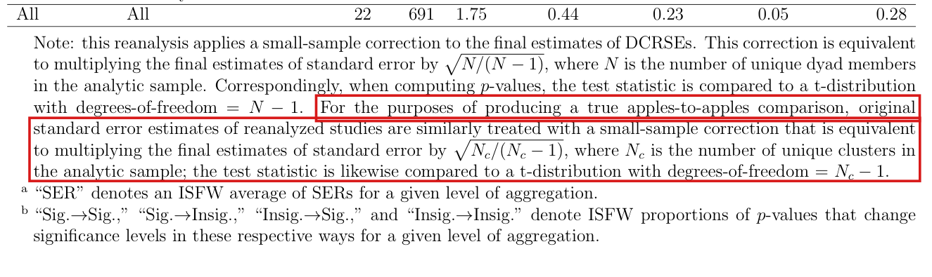
In the small-sample reanalysis behind Supplementary Table A.5, the code does not apply the stated correction to the original standard errors of the three Arel-Bundock (2017) models, and it takes the degrees of freedom for four Pratt (2018) models from clusters counted before observations are dropped.

Note to Supplementary Table A.5, Supplementary Appendix p. A5 (PDF p. 5), sentence beginning “For the purposes of producing a true apples-to-apples comparison”; cited in footnote 12, p. 193 (PDF p. 8); replication file code/dof_corrections/2_reanalysis_r_dof.R, lines 87–101 and 151–179

As printed

Table A.5, note. For the purposes of producing a true apples-to-apples comparison, original standard error estimates of reanalyzed studies are similarly treated with a small-sample correction that is equivalent to multiplying the final estimates of standard error by Nc/(Nc−1)\sqrt{N_c/(N_c-1)}, where NcN_c is the number of unique clusters in the analytic sample; the test statistic is likewise compared to a t-distribution with degrees-of-freedom =Nc−1=N_c-1.

Replication file, lines 88 and 90 (Arel-Bundock, model 1; models 2 and 3 are alike).

original_se = sqrt(diag(vcovHC(m1_arelbundock2017, type = "HC0"))),

df_ori = nobs(m1_arelbundock2017) - 1,

Replication file, line 154 (Pratt, model 1; models 2 to 6 are alike).

df_ori = length(unique(spec1_data_pratt2018$Dir.DyadID)) - 1,

The problem

The note describes two steps for the original standard errors, and the R script for this reanalysis departs from each. For the three Arel-Bundock (2017) models the original standard error is the HC0 standard error, and no factor is applied. Under HC0 each observation is its own cluster. This implies that NcN_c is the number nn of observations in the fit, and the note calls for the factor n/(n−1)\sqrt{n/(n-1)}. For the Pratt (2018) models the degrees of freedom are one less than the number of clusters in the data frame passed to the fit. The fit drops rows with missing values, and the clusters that remain are fewer in models 1, 2, 3 and 5.

Two other points qualify the comparison and are not counted as errors. The original standard errors for Pratt (2018) come from sandwich::vcovCL, whose defaults already supply G/(G−1)G/(G-1) for GG clusters, and (n−1)/(n−k)(n-1)/(n-k) in the least-squares fits. For the Stata studies the command multiplies the refitted original covariance by Nc/(Nc−1)N_c/(N_c-1), as the note says. For Shelef (2016) that covariance already carries {G/(G−1)}{(n−1)/(n−k)}\{G/(G-1)\}\{(n-1)/(n-k)\}, and the cluster factor enters twice.

Evidence an exact counterexample

The evidence is an exact example run through the script’s own function and a refit of the Pratt models. Let x=(0,1,2,3)x=(0,1,2,3) and y=(0,1,1,3)y=(0,1,1,3), and consider the least-squares fit with an intercept. The coefficients are (−1/10, 9/10)(-1/10,\,9/10) and the residuals are (1/10, 1/5, −7/10, 2/5)(1/10,\,1/5,\,-7/10,\,2/5). A direct computation gives

VHC0=(113/5000−21/2500−21/2500103/5000),43 VHC0=(113/3750−7/625−7/625103/3750).V_{\mathrm{HC0}}=\begin{pmatrix}113/5000&-21/2500\\-21/2500&103/5000\end{pmatrix},\qquad \frac{4}{3}\,V_{\mathrm{HC0}}=\begin{pmatrix}113/3750&-7/625\\-7/625&103/3750\end{pmatrix}.

The function reg_table of the script returns the standard errors 0.15030.1503 and 0.14350.1435 from the first matrix, while the note with Nc=n=4N_c=n=4 requires 0.17360.1736 and 0.16570.1657 from the second. In general the squared ratio of the two is (n−1)/n(n-1)/n. For the first model of Arel-Bundock (2017), with n=3971n=3971 (Supplementary Table A.1), the missing factor is 3971/3970≈1.000126\sqrt{3971/3970}\approx 1.000126.

For Pratt (2018), refitting models 1 to 5 on the data in the replication files and counting the clusters among the fitted rows, I obtain the following.

Pratt (2018), models 1–5: clusters and original degrees of freedom.
ModelRows in fitClusters, all rowsClusters, fitdf in scriptdf by the note
11177238209237208
21177238209237208
32025329290328289
43718329329328328
53343329328328327

The pp-value of the KEV in model 1 is 0.077480.07748 with 237237 degrees of freedom and 0.077660.07766 with 208208. No KEV in these five models crosses the 5% level when the degrees of freedom are corrected. Model 6 was not refitted.

What survives

This finding does not contradict the DCRSEs, the primary analysis in Table 5, or the statement of footnote 12 that the small-sample reanalysis shows no substantive differences. The two corrections bear on Table A.5 alone. There the original standard errors of the first model of Arel-Bundock (2017) grow by a factor of about 1.00011.0001, and the original pp-values of the KEVs in models 1 to 5 of Pratt (2018) move by less than 0.00020.0002. A corrected Table A.5 has not been computed.

Corrected

In 2_reanalysis_r_dof.R, for each of the three Arel-Bundock (2017) models, the original standard error is n/(n−1)\sqrt{n/(n-1)} times the HC0 standard error, where nn is nobs(model). For each Pratt (2018) model, the original degrees of freedom are Nc−1N_c-1, where NcN_c is the number of distinct values of Dir.DyadID in the source-data rows matched by row name to model.frame(model). This gives 208208, 208208, 289289, 328328 and 327327 degrees of freedom for models 1 to 5. Table A.5 is then recomputed.

The note to Table A.5 should also state which finite-sample factors each original standard error carries. After the two changes these are the HC0 standard error times n/(n−1)\sqrt{n/(n-1)} for Arel-Bundock (2017); the sandwich::vcovCL defaults for Pratt (2018), with no further factor; and, for the Stata studies, the covariance returned by the original command times Nc/(Nc−1)N_c/(N_c-1).

Crop of the last row of Table A.5 and the note below it. A red outline marks the sentence that begins: For the purposes of producing a true apples-to-apples comparison, original standard error estimates of reanalyzed studies are similarly treated with a small-sample correction. The sentence ends: degrees-of-freedom equals N sub c minus 1.
Supplementary Appendix, p. A5 (PDF p. 5), note to Table A.5. The marked sentence says that the original standard errors receive the factor Nc/(Nc−1)\sqrt{N_c/(N_c-1)} and a tt reference distribution with Nc−1N_c-1 degrees of freedom, where NcN_c counts the clusters in the analytic sample.

The cross-reference “section 3” should read “Table 3”.

First paragraph below Table 4, second sentence, p. 190 (PDF p. 5)

As printed

With the same six observations, section 3 demonstrates the additional clustering permitted.

The problem

The passage points to a section instead of the covariance table used in its comparison. The sentence stands in Section 3 and introduces the covariance structure assumed under clustering by repeated dyad, which Table 3 displays.

Evidence a check of the printed page

I checked the page. The next paragraph begins “In Table 3”, and the parallel sentence on p. 189 reads “Table 2 demonstrates”.

What survives

The covariance comparison is unaffected by the wrong cross-reference.

Corrected

With the same six observations, Table 3 demonstrates the additional clustering permitted.

Four lines of text. In the second line a red box surrounds the link 'section 3', in the sentence 'With the same six observations, section 3 demonstrates the additional clustering permitted.' The fourth line begins the next paragraph with 'In Table 3, we can see that'.
First paragraph below Table 4, p. 190 (PDF p. 5), with the first line of the next paragraph. The mark is on “section 3”.

The article by Erikson, Pinto, and Rader was published in 2014, not 2017.

References, p. 197 (PDF p. 12), entry for Erikson, Pinto, and Rader; citations on pp. 186–187 (PDF pp. 1–2)

As printed

p. 197. Erikson, R. S., P. M. Pinto, and K. T. Rader. 2017. “Dyadic Analysis in International Relations: A Cautionary Tale.” Political Analysis 22 (4): 457–463.

pp. 186–187. “Erikson, Pinto, and Rader (2017)”; “Erikson et al. (2017)”; “Erikson et al. 2017”.

The problem

Volume 22, issue 4 of Political Analysis is the Autumn 2014 issue. The publisher’s page for the article also carries the line “Published online by Cambridge University Press: 04 January 2017”, and that date is not the year of the journal issue.

Evidence a check of the printed page

The evidence is a check of the publisher’s page for the article, https://doi.org/10.1093/pan/mpt051, which gives Volume 22, Issue 4, Autumn 2014, pp. 457–463. In the same reference list, Political Analysis 23 (4) is dated 2015 and 24 (4) is dated 2016.

What survives

The article is identified correctly by its authors, title, volume, issue and pages; only the year changes, in the reference and in its three citations.

Corrected

p. 197. Erikson, R. S., P. M. Pinto, and K. T. Rader. 2014. “Dyadic Analysis in International Relations: A Cautionary Tale.” Political Analysis 22 (4): 457–463.

pp. 186–187. “Erikson, Pinto, and Rader (2014)”; “Erikson et al. (2014)”; “Erikson et al. 2014”.

Crop of three entries of the reference list. A red outline marks the year 2017 in the entry: Erikson, R. S., P. M. Pinto, and K. T. Rader. 2017. Dyadic Analysis in International Relations: A Cautionary Tale. Political Analysis 22 (4): 457 to 463.
p. 197 (PDF p. 12), reference list. The marked year in the entry for Erikson, Pinto, and Rader is 2017; the entry places the article in volume 22, issue 4.

The nine reanalyzed models of Shelef (2016) have region-by-decade indicators and no fixed effect for either dyad member; two studies, not three, have a model with fixed effects for both members of the dyad, and the Shelef row does not belong in Supplementary Table A.4.

Section 4, p. 192 (PDF p. 7), sentence beginning “Three studies employ”, and footnote 10; Supplementary Table A.4, row Shelef (2016), p. A4 (PDF p. 4 of the supplement)

As printed

P. 192: “Three studies employ at least one model that has fixed effects for both members of the dyad under consideration.”

Footnote 10, p. 192: “Supplementary Table A.4 shows the results of applying DCRSEs to the KEVs in these three papers.”

Supplementary Table A.4, p. A4:

Table A.4: Reanalysis for Models with Fixed Effects for both Dyad Members
StudyKEVsSig.→\toSig.Sig.→\toInsig.Insig.→\toSig.Insig.→\toInsig.Avg. SER
Carter and Poast (2020)80.000.380.500.121.10
Shelef (2016)90.890.000.000.111.07
Bermeo and Leblang (2015)11.000.000.000.002.13
The problem

Each of the nine Shelef regressions behind this row has one set of indicators, i.regionfe_region_decade, and no indicators for the state that loses territory (loseccode) or for the state that gains it (gainccode). The first of them reads

reg midpost homelandclaim priormid coethnicity oil_gas capital_distance_log dyaddem allydummy cincrat i.regionfe_region_decade if colony2==0, cluster(dyadid4)

The options dm1(loseccode) and dm2(gainccode) of the DCR command name the dyad members for the variance and add no regressors. Region-by-decade indicators do not contain the member effects. These models are not models with fixed effects for both members of the dyad, and the subgroup that p. 192 and footnote 10 describe has two studies.

Evidence an exact counterexample

The evidence is an exact check on the data of the replication files. Observations 3 and 7 of the Shelef data file are in the estimation sample of all nine models and have the same level, 7, of regionfe_region_decade. Their members are (255,315)(255,315) and (315,260)(315,260), with the losing state first. Let ww be the vector with +1+1 on observation 3, −1-1 on observation 7 and 00 elsewhere. Then ww is orthogonal to every indicator of regionfe_region_decade. Its inner product with the indicator of losing state 255 is 11, and the same holds for the indicator of gaining state 315 and for the indicator that state 255 is either member. This implies that none of these three indicators is a linear combination of the region-by-decade indicators. The other regressors cannot supply the member effects either. In the three groups of models (Tables 3, 4 and 5 of the study) the design matrix has rank at most 34, 31 and 33. The indicators of the losing and of the gaining states have ranks 114 and 114, 105 and 104, and 83 and 83.

What survives

The numbers of the Shelef row are those of the nine models as fitted. I did not recompute them, and no error in them is shown. Shelef (2016) stays in the primary analysis of 22 studies, and Table 5 and Supplementary Tables A.1 and A.2 do not change. What changes is the subgroup with fixed effects for both members. It has two studies and 9 KEVs (8+18+1), not three studies and 18. The article draws no conclusion from this subgroup.

Corrected

P. 192: “Two studies employ at least one reanalyzed model that has fixed effects for both members of the dyad under consideration.”

Footnote 10: “Supplementary Table A.4 shows the results of applying DCRSEs to the KEVs in these two papers.”

Supplementary Table A.4 keeps its title and the rows Carter and Poast (2020) and Bermeo and Leblang (2015). The row Shelef (2016) is removed, and shelef2016_FE is removed from FE_papers in 3_reanalysis_merge.R (lines 824–828).

Crop of five lines of page 192. A red box marks the words 'Three studies' at the start of the sentence 'Three studies employ at least one model that has fixed effects for both members of the dyad under consideration', which carries the footnote mark 10.
Section 4, p. 192 (PDF p. 7). The marked count includes Shelef (2016), whose reanalyzed models have no fixed effect for either dyad member.
The whole of Table A.4, Reanalysis for Models with Fixed Effects for both Dyad Members, with three rows. A red box marks the second row: Shelef (2016), 9 KEVs, 0.89, 0.00, 0.00, 0.11, Avg. SER 1.07. The other rows are Carter and Poast (2020) and Bermeo and Leblang (2015).
Supplementary Table A.4, p. A4 (PDF p. 4 of the supplement). The marked row is computed from models with region-by-decade indicators only.
Crop of footnote 10 on page 192, between the last line of footnote 9 and the first line of footnote 11. A red box marks the words 'three papers' at the end of the sentence 'Supplementary Table A.4 shows the results of applying DCRSEs to the KEVs in these three papers'.
Footnote 10, p. 192 (PDF p. 7), which repeats the count.

The stated minimum of Stata 15 does not hold for the conditional-logit path of the dcr command, because the supplied nclogit program requires Stata 16.1 or higher.

Data Availability Statement, p. 196 (PDF p. 11); the same sentence in the Supplementary Appendix, “Statistical Programming Suite”, p. A1 (PDF p. 1)

As printed

p. 196 and Supplementary Appendix, p. A1. To access the source code for the dcr command for Stata (version 15 or higher), clone its GitHub repository:

nclogit.ado, lines 1–2.

program nclogit, eclass

version 16.1

The problem

The program nclogit, supplied with dcr for conditional-logit models, begins with the statement version 16.1, which is executed before any argument is read. Stata 15 and 15.1 cannot run a program that requests a later version. Every call of dcr nclogit stops at that statement, although dcr.ado itself declares version 15. The replication uses this path for three models, one of Weisiger and Yarhi-Milo (2015) and two of Kinne (2018).

Evidence a derivation

The evidence is a reading of the source of dcr.ado and of nclogit.ado, whose two released copies are identical, together with the rule for Stata’s version command. Stata was not run.

What survives

Results produced with Stata/MP 17.0, the version named in the replication README, are unaffected, and no estimate, table or figure changes. The other estimator paths of dcr are not shown to fail on Stata 15.

Corrected

p. 196 and Supplementary Appendix, p. A1. To access the source code for the dcr command for Stata (the dcr wrapper declares version 15; the supplied nclogit conditional-logit path requires version 16.1 or higher), clone its GitHub repository:

Crop of the first four lines of the Data Availability Statement. A red outline marks the words: command for Stata (version 15 or higher). The next line is the command git clone git@github.com:jscarlson/stata-dcr.git.
p. 196 (PDF p. 11), Data Availability Statement. The marked words give Stata 15 as the minimum version for the dcr command.

The number of observations for Schneider and Tobin (2020) in Supplementary Table A.1 is 952, not 4760, and the 756 dyads of that row are directed donor–recipient pairs.

Supplementary Table A.1, row “Schneider and Tobin (2020)”, supplement p. A2 (PDF p. 2 of the Supplementary Appendix)

As printed

Table A.1: Dyadic Data Summary Statistics, Study Level. The columns are Study, Observations, Data Start Year, Data End Year and Number of Unique Dyads, and the row reads:

Schneider and Tobin (2020), 4760, 1976, 2009, 756.

Note: summary statistics for each study computed using data from a representative (usually the first) reanalyzed model, as analytic samples and data often vary by model.

The problem

The note to the table says that the statistics come from a representative reanalyzed model. The three reanalyzed models of this study are fitted to 952 donor–recipient–year observations. The printed 4760 equals 5×9525\times952, and the code in the replication files requests five imputations. The entry has the size of five completed copies of the sample and does not count the observations once. The entry 756 is the number of directed donor–recipient pairs among the 952 observations. With direction ignored, as in the clustering of the reanalysis (p. 192), there are 741 pairs, and the table does not say which convention it uses.

Evidence a recalculation from the source

The evidence is a recalculation from the replication files. The data file has 4624 rows, of which 952 satisfy the condition g7==1 of the three models. Each of these is a distinct donor–recipient–year, and the years run from 1976 to 2009. The 96 saved pp-values that use a tt distribution (two columns for each of 16 coefficients in three models) are reproduced with n=952n=952 and 936 degrees of freedom to within 2.8×10−162.8\times10^{-16}, and not with n=4760n=4760. The 952 observations contain 756 distinct ordered pairs and 741 unordered pairs: 15 pairs of countries occur in both orders, and six of the 741 pair a country with itself. The code that filled the summary workbook is not in the replication files, and how the entry 4760 was produced cannot be traced.

What survives

The correction changes this row of Table A.1 and the corresponding cells of the summary workbook in the replication files. The years 1976 and 2009 are correct, and 756 is correct as a count of directed pairs. The estimates, standard errors, standard error ratios and significance comparisons are computed from the model outputs and do not use these two columns.

Corrected

Schneider and Tobin (2020), 952, 1976, 2009, 756.

For Schneider and Tobin (2020), 756 counts directed donor–recipient pairs. Ignoring direction, there are 741 pairs, six of which pair a country with itself.

The title 'Table A.1: Dyadic Data Summary Statistics, Study Level' and the header row 'Study, Observations, Data Start Year, Data End Year, Number of Unique Dyads', then a dashed grey rule, then seven rows from Pratt (2018) to Weisiger and Yarhi-Milo (2015) and the note below the table. The row 'Schneider and Tobin (2020)' reads 4760, 1976, 2009, 756, and a red box surrounds 4760.
Supplementary Table A.1, supplement p. A2: the title and header, the last seven rows and the note, with the fifteen rows between them left out at the dashed rule. The mark is on the number of observations for Schneider and Tobin (2020).

For the one study fitted to multiply imputed data, the code removes the finite-sample corrections from covariance matrices that are already pooled over the imputations, which also rescales the between-imputation component; the result need not equal the DCR covariance computed within each imputation and then pooled.

Replication files: 1_reanalysis_stata.do, lines 1375, 1380 and 1385, and stata-dcr/dcr.ado, lines 125–238. The results enter Supplementary Table A.2, row “Schneider and Tobin (2020)”, supplement p. A3 (PDF p. 3 of the Supplementary Appendix). The article prints no statement on multiple imputation.

See also under Formal statements (Lean): P032-T8, P032-T9

As printed

Line 1375 of 1_reanalysis_stata.do, with the regressors and the output path left out:

dcr logit bilateral_bailout … if g7==1, dm1(cc) dm2(dc) crse(donor_country) psd dofundo(asylike) syntax(vce) xlsxpath(…) prefix(mi estimate, post:)

Lines 145, 154 and 157 of stata-dcr/dcr.ado, for the repeated-dyad component:

matrix vrep = e(V)

scalar unadjust = ((N_did - 1)/N_did)

matrix vcov = -1*unadjust*vrep

The 18 key explanatory variables (KEVs) of the three models give the row of Supplementary Table A.2: Schneider and Tobin (2020), 18, 0.333, 0, 0.056, 0.611, 0.999.

The problem

Each of the three calls runs every component of the decomposition on p. 191 under the prefix mi estimate, post:. Under the standard behaviour of this prefix, the matrix e(V) returned for a component is the covariance pooled over the five imputations by Rubin’s rules: the average of the within-imputation covariances plus (1+1/M)B(1+1/M)B, where BB is the between-imputation covariance of the coefficients and M=5M=5. The command then multiplies the returned matrix by the factor that removes the finite-sample correction of that component. This factor belongs to the within-imputation covariance only. Applied to the pooled matrix, it also multiplies (1+1/M)B(1+1/M)B. The components carry different factors, and the between-imputation term enters the result with a coefficient cc that differs from 1 in general. The DCR covariance computed within each imputation and then pooled has coefficient 1. The decomposition on p. 191 is correct for one complete data set if no same-country dyad appears in more than one observation.

Evidence an exact counterexample

The evidence is a derivation from the code and an exact counterexample. No Stata run was made, and the three models were not refitted. Let KK be the number of dyad members (the NN of p. 191), nn the number of observations and MM the number of imputations. The decomposition has one component for each member ii, the repeated-dyad component DD and the heteroskedasticity-consistent component 00, with signed weights si=1s_i=1, sD=−1s_D=-1 and s0=−(K−2)s_0=-(K-2), so that ∑jsj=1\sum_js_j=1. For component jj, let Uˉj\bar U_j be the average over the imputations of the within-imputation covariance without finite-sample correction, and let aja_j be the factor by which the command multiplies. The corrected within-imputation covariance is the uncorrected one divided by aja_j. Suppose that no same-country dyad appears in more than one observation, that the sample, the clusters and the factors are the same in every imputation and that no eigenvalue adjustment is made. Since the fitted coefficients do not depend on the clustering, every component has the same Q=(1+1/M)BQ=(1+1/M)B. The matrix returned for component jj is Tj=Uˉj/aj+QT_j=\bar U_j/a_j+Q, and the command computes

Tcode=∑jsjajTj=∑jsjUˉj+cQ,c=∑jsjaj.T_{\mathrm{code}}=\sum_js_ja_jT_j=\sum_js_j\bar U_j+cQ,\qquad c=\sum_js_ja_j.

The DCR covariance computed within each imputation and then pooled is T∗=∑jsjUˉj+QT_*=\sum_js_j\bar U_j+Q. Subtracting, I find Tcode−T∗=(c−1)(1+1/M)BT_{\mathrm{code}}-T_*=(c-1)(1+1/M)B. With the option dofundo(asylike), the factors are ai=1−1/Gia_i=1-1/G_i, aD=1−1/GDa_D=1-1/G_D and a0=1−1/na_0=1-1/n, where GiG_i and GDG_D are the numbers of clusters in the component for member ii and in the repeated-dyad component. Substituting these factors into the definition of cc, I obtain

c−1=−∑i=1K1Gi+1GD+K−2n,c-1=-\sum_{i=1}^{K}\frac{1}{G_i}+\frac{1}{G_D}+\frac{K-2}{n},

which is not zero in general.

The decomposition includes each observation paired with itself; it omits only pairs of different observations on a common same-country dyad. In the source data, I count each of the six same-country dyads just once among the 952 observations with g7==1, so none contributes such an omission.

For the counterexample, I consider 24 observations, four on each of the six dyads among four members, an intercept-only logit and five imputations. Three imputations complete the data to 12 successes and two to 18. Then K=4K=4, n=24n=24, GD=6G_D=6 and Gi=13G_i=13 for every member, and c=4(12/13)−5/6−2(23/24)=49/52c=4(12/13)-5/6-2(23/24)=49/52. The fitted intercepts are 00 and log⁡3\log3, and I have B=3(log⁡3)2/10B=3(\log3)^2/10 and Q=9(log⁡3)2/25Q=9(\log3)^2/25. The DCR variances within the two kinds of imputation are 2/92/9 and 8/818/81, with average 14/8114/81. A direct computation gives T∗=14/81+(9/25)(log⁡3)2T_*=14/81+(9/25)(\log3)^2 and Tcode=14/81+(441/1300)(log⁡3)2T_{\mathrm{code}}=14/81+(441/1300)(\log3)^2, and the difference is −(27/1300)(log⁡3)2<0-(27/1300)(\log3)^2<0. All the variances are positive, and the eigenvalue adjustment is not active.

What survives

The decomposition on p. 191 is unaffected. The reanalyses of the other 21 studies do not use this multiple-imputation prefix. The logit coefficients of the three models are unaffected, since the covariance estimator does not change them. The DCR covariance of the three models depends on this code, and with it the DCRSEs, the standard error ratios and the DCR pp-values of the 18 KEVs in the row of Supplementary Table A.2. These enter the 2020, IPE and overall rows of Table 5 and Figures 1–3, and the same calls are repeated in the small-sample reanalysis behind Supplementary Table A.5. No value in these tables is shown to be wrong. The size and direction of the difference for the three models have not been computed, because the replication files do not keep the coefficient and covariance matrices of each imputation.

Corrected

For a model fitted to MM imputed data sets, the DCR covariance is computed as follows.

  1. In each imputation mm, compute each component covariance and remove its finite-sample correction with the factor of that component, taken from the sample and the clusters of that imputation. If no same-country dyad appears in more than one observation, form
    V^r(m)=∑i=1KV^c,i(m)−V^D(m)−(K−2)V^0(m).\widehat V_r^{(m)}=\sum_{i=1}^{K}\widehat V_{c,i}^{(m)}-\widehat V_D^{(m)}-(K-2)\widehat V_0^{(m)}.
    If a same-country dyad is observed more than once, compute V^r(m)\widehat V_r^{(m)} by the direct sandwich sum over observation pairs whose dyads share a member, including an observation paired with itself.
  2. Pool by Rubin’s rules, with the between-imputation term entering once and with coefficient 1:
    V^r=1M∑m=1MV^r(m)+(1+1M)B.\widehat V_r=\frac{1}{M}\sum_{m=1}^{M}\widehat V_r^{(m)}+\colorbox{#ffe58a}{$\displaystyle \Bigl(1+\frac{1}{M}\Bigr)B$}.
  3. Apply the eigenvalue adjustment of footnote 3, where it is used, at a stated point of this sequence.

When no same-country dyad appears in more than one observation, the sample, the clusters and the factors are the same in every imputation and no eigenvalue adjustment is active, the result equals the matrix that the code now computes plus (1−c)(1+1/M)B(1-c)(1+1/M)B, with cc as in the evidence above. The option dofundo(none) is not a repair, since it leaves the finite-sample corrections in the within-imputation components. The three models and the summaries that use them are then to be recomputed.

A listing of Stata code with line numbers. Line 1375 of 1_reanalysis_stata.do is a call 'dcr logit bilateral_bailout ...' that wraps over six rows; red outlines surround 'dofundo(asylike)' and 'prefix(mi estimate, post:)' in its options. Below, lines 125 to 127 of dcr.ado run the prefixed command with vce(cluster did), line 145 reads 'matrix vrep = e(V)', lines 153 to 155 set 'scalar unadjust = ((N_did - 1)/N_did)' when dofundo is asylike, and line 157 reads 'matrix vcov = -1*unadjust*vrep', with a red outline around 'unadjust*vrep'.
Source code of the replication files, not a page of the article: 1_reanalysis_stata.do, line 1375, and stata-dcr/dcr.ado, lines 125–127, 145 and 153–157. The outlines mark the option that removes the finite-sample correction, the multiple-imputation prefix, and the product of the factor with the matrix returned under that prefix.
The title 'Table A.2: Primary Results, Study Level' and the header row 'Study, Subfield, Secondary Subfield, Primary Relationship Tested, KEVs, Sig. to Sig., Sig. to Insig., Insig. to Sig., Insig. to Insig., Avg. SER', then a dashed grey rule, then the rows from Pratt (2018) to Weisiger and Yarhi-Milo (2015) and the row 'Average-of-Averages (= ISFW)'. A red box surrounds the row 'Schneider and Tobin (2020), IPE, International finance, Domestic spillovers and international bailout, 18, 0.333, 0, 0.056, 0.611, 0.999'.
Supplementary Table A.2, supplement p. A3: the title and header, the last seven study rows and the row of averages, with the fifteen rows between them left out at the dashed rule. The marked row holds the results that pass through this code. No entry of the row is shown to be wrong.

Clarity notes

Imprecise or ambiguous wording whose intended meaning is correct; not an error.

The six observations of Tables 2–4 stand for three dyads, each observed twice, of which the middle one shares a member with each of the other two; with the indices of p. 189, the labels 111, 112, 221 and 222 pair a country with itself.

Tables 2, 3 and 4, row and column labels, p. 190 (PDF p. 5)

See also under Formal statements (Lean): P032-T11

As printed

In each of Tables 2–4 the header is ijt / i′j′t′ijt\,/\,i'j't', and the rows and columns are labelled 111, 112, 211, 212, 221, 222. Table 4, for example, has E[u111u112]\mathrm{E}[u_{111}u_{112}] in the cell (111,112)(111,112), E[u221u222]\mathrm{E}[u_{221}u_{222}] in the cell (221,222)(221,222), and 00 in the cells that pair 111 or 112 with 221 or 222.

Intended meaning

Page 189 defines YijtY_{ijt} as the level of commerce between countries ii and jj in period tt. With these indices, the printed labels are the dyads (1,1)(1,1), (2,1)(2,1) and (2,2)(2,2) in periods 1 and 2, and two of the three pair a country with itself. The tables are a schematic of three pairs of countries, each observed twice, in which the middle pair shares a member with each outer pair and the outer pairs share none. The zero pattern of each table is correct for this picture, and also for the labels as printed. The labels matter only if the illustration is carried to the decomposition on p. 191. For a dyad that pairs a member with itself, the decomposition gives weight 0 to the covariance between its two observations, where Table 4 has a nonzero entry. With distinct members, the decomposition agrees with Table 4 in all 36 cells.

Corrected

In Tables 2–4, replace the row and column labels, and the matching subscripts of uu, as follows: 111 by 121, 112 by 122, 211 by 131, 212 by 132, 221 by 341 and 222 by 342. The observations are then the dyads (1,2)(1,2), (1,3)(1,3) and (3,4)(3,4), each in two periods, and every zero and nonzero entry of the three tables is unchanged.

A table titled 'Table 4. Dyadic clustering.' with header cell 'ijt / i-prime j-prime t-prime' and six columns and six rows labelled 111, 112, 211, 212, 221, 222. A red box surrounds the six column labels and a second red box surrounds the six row labels. The cells contain expectations of products of residuals, such as E[u_111 u_112], except that the four cells pairing rows 111 and 112 with columns 221 and 222, and the four cells pairing rows 221 and 222 with columns 111 and 112, contain 0.
Table 4, p. 190 (PDF p. 5). The column labels and the row labels are marked; Tables 2 and 3 on the same page carry the same labels.

The decomposition does not say what NN is, nor how V^c,i\widehat V_{c,i} treats the observations whose dyad does not contain member ii: NN is the number of unique dyad members, and each such observation is its own cluster.

Display for V^r\widehat V_r and the sentence that defines its terms, p. 191 (PDF p. 6)

See also under Formal statements (Lean): P032-T11

As printed

V^r=∑i=1NV^c,i−V^D−(N−2)V^0,\widehat V_r=\sum_{i=1}^{\colorbox{#ffe58a}{$\displaystyle \scriptstyle N$}}\widehat V_{c,i}-\widehat V_D-(\colorbox{#ffe58a}{$\displaystyle N$}-2)\widehat V_0,

where V^r\widehat V_r is the estimated DCR variance–covariance matrix for longitudinal data; V^c,i\widehat V_{c,i} is the estimated dyad-member-ii-specific clustered variance–covariance matrix; V^D\widehat V_D is the estimated repeated-dyad clustered variance–covariance matrix; and V^0\widehat V_0 is the estimated heteroskedasticity-consistent variance–covariance matrix.

Intended meaning

NN is the number of unique dyad members, as the note to Supplementary Table A.5 says. In V^c,i\widehat V_{c,i} all observations whose dyad contains member ii form one cluster, which footnote 2 indicates, and every other observation is a cluster by itself. The pieces carry no finite-sample factors, and each dyad has two distinct members. With these definitions the display is an exact identity. In ∑iV^c,i\sum_i\widehat V_{c,i} the square of an observation appears NN times, the product of two observations of the same dyad twice, and the product of two observations whose dyads share one member once. Subtracting V^D\widehat V_D and (N−2)V^0(N-2)\widehat V_0 leaves each of these exactly once. The R package uses these definitions.

Corrected

After the display and its definitions, add: Here NN is the number of unique dyad members. In V^c,i\widehat V_{c,i}, all observations whose dyad contains member ii form one cluster and each remaining observation forms its own singleton cluster. The components use the same unadjusted sandwich convention, and each dyad contains two distinct members.

Crop of the top of page 191: two lines of text, the displayed equation for V hat r, and the paragraph that defines its terms. Two small red boxes mark the letter N, once as the upper limit of the sum and once inside the bracket (N minus 2). Two more red boxes mark the words 'V hat c,i is the estimated dyad-member-i-specific clustered variance-covariance matrix', which run over two lines.
The decomposition on p. 191 (PDF p. 6). The marked symbol NN is not defined on the page, and the marked definition of V^c,i\widehat V_{c,i} does not say how the remaining observations are clustered.

A SER different from one need not come from inter-dyad dependence alone: the DCRSE receives no small-sample correction, while the original standard error keeps the finite-sample factors of its software.

Section 4, pp. 192–193 (PDF pp. 7–8), sentence beginning “Also, for the purposes of our primary reanalysis”; Section 4.1, p. 193 (PDF p. 8), definition of the SER and footnote 13

As printed

pp. 192–193. Also, for the purposes of our primary reanalysis, there are no small-sample corrections made to our standard error estimates. Finite-sample corrections would inflate our standard error estimates to account for increased sampling variability, and thus might paint an overly pessimistic picture of the original literature.

p. 193. We compute a standard error ratio (SER) for all KEVs, which is the DCRSE divided by the standard error produced using the original variance estimation strategy.

p. 193, footnote 13. For example, if the original model clustered standard errors on repeated dyads, the SER is a ratio of DCR standard error to repeated dyad clustered standard error. The SER can therefore be interpreted as the inflation (or deflation) of the original standard error introduced by inter-dyad dependencies.

Intended meaning

The phrase “our standard error estimates” refers to the DCRSEs, which receive no final small-sample correction in the primary reanalysis. The SER is computed as defined, and the comparison with the original standard errors is the one the paper intends. The denominator is the standard error that the replication software returns, and it keeps that software’s finite-sample factors. In the nine least-squares models of Shelef (2016), the clustered variance of the original fit carries the factor q={G/(G−1)}{(n−1)/(n−k)}q=\{G/(G-1)\}\{(n-1)/(n-k)\} for nn observations, GG clusters and design rank kk, while the DCR variance is constructed from components with their finite-sample factors removed. If RR denotes the published ratio, then the ratio with no factor on either side is q R\sqrt{q}\,R, and the published ratio is the smaller of the two since q>1q>1. For Shelef (2016) the mean of RR is 1.0711.071, as in Supplementary Table A.2, and the mean of q R\sqrt{q}\,R is 1.1491.149. An exact example shows that the factor alone can move the ratio. Suppose that each of the six dyads among four members has one observation, that the fit has an intercept only, and that the outcomes are (1,0,0,0,0,−1)(1,0,0,0,0,-1) on the dyads (1,2),(1,3),(1,4),(2,3),(2,4),(3,4)(1,2),(1,3),(1,4),(2,3),(2,4),(3,4). The two nonzero residuals lie on disjoint dyads. Then both variances without factors equal 1/181/18 and the original variance with q=6/5q=6/5 is 1/151/15, and I obtain 5/6≈0.913\sqrt{5/6}\approx 0.913 for the SER. No revised average over the 22 studies has been computed, and the reported ratios stand as defined.

Corrected

pp. 192–193. Also, for the purposes of the primary reanalysis, no final small-sample correction is made to the DCR standard error estimates; the original standard errors keep the finite-sample adjustments returned by the replication software.

p. 193, footnote 13. For example, if the original model clustered standard errors on repeated dyads, the SER is a ratio of DCR standard error to repeated dyad clustered standard error. The SER therefore measures the inflation (or deflation) of the original standard error under DCR re-estimation; it reflects the additional inter-dyad covariance terms and any difference in finite-sample adjustment between the two standard errors.

Crop of footnotes 12, 13 and 14 at the foot of page 193. A red outline marks the second sentence of footnote 13: The SER can therefore be interpreted as the inflation (or deflation) of the original standard error introduced by inter-dyad dependencies.
p. 193 (PDF p. 8), footnotes 12–14. The marked sentence of footnote 13 attributes the whole ratio to inter-dyad dependencies.

Formal statements (Lean)

Formal results: 10 whole; 2 restricted; 0 refuted; 0 omitted.

Coverage concerns the identified claim under its stated assumptions. A checked proof establishes the formal statement; correspondence to the published text was reviewed by AI. Repository access is currently required to open the source links.

Each result links to its current formal statement and proof. “Whole” covers the identified claim under its assumptions; “restricted” covers the stated narrower scope; “refuted” gives a counterexample to the identified assertion; “omitted” has no current theorem. Any named published theorem used as a premise remains an assumption. Browse the formal results for this work.

The decomposition as it must be implemented, with every hypothesis: record-level V^0\hat V_0 and common scores, bread and scaling in all components; and the exact discrepancy when an id-clustered matrix is subtracted instead

p. 191 (PDF p. 6), display for V^r\hat V_r and the sentence defining its terms; dcr.ado lines 108–119 and 163–190

p. 191 display and component definitions; dcr.ado lines 108–119 and 163–190. Common scores give the exact decomposition and exhaustive coefficient count, while subject-id substitution and arbitrary residual scaling have the stated discrepancies.

Historical component credits
  • Proved AronowAudit.P032.dyad_intersection_cases Historical support retained; baseline fidelity: ok; manifest: used; used in Solution; Auxiliary cardinality fact expressly included in T4(ii). Allowing an arbitrary ambient member type changes none of the finite-member cases needed by the target.
  • Proved AronowAudit.P032.decomposition_coefficient Historical support retained; baseline fidelity: ok; manifest: used; used in Solution; Auxiliary pointwise coefficient identity for T4(ii); the sum over members uses a finite member type, and N is cast to real before subtraction. Its four cases follow directly from the definitions and the two-member property.
  • Proved AronowAudit.P032.corrected_decomposition Historical support retained; baseline fidelity: ok; manifest: used; used in Solution; Establishes T4(i,v) for arbitrary common scores, with outsider singleton contributions and unused members exactly as permitted by the target. No covariance signs, rank, score equations or statistical model are assumed.
  • Proved AronowAudit.P032.id_substitution_discrepancy Historical support retained; baseline fidelity: ok; manifest: used; used in Solution; The sole mathematical difference is a valid generalization: Vid may be any real matrix. Specializing Vid to scoreSandwich(idPattern g,z) recovers exactly T4(iv), with alpha arbitrary; no claim-stage verdict changed after reading the record.
  • Proved AronowAudit.P032.id_cross_products Historical support retained; baseline fidelity: ok; manifest: used; used in Solution; Establishes the record-plus-cross-product identity used in T4(iii); offIdPattern excludes precisely r=s, so all remaining within-id ordered products, in both orders, are present.
  • Proved AronowAudit.P032.singleton_id_covariance Historical support retained; baseline fidelity: ok; manifest: used; used in Solution; The injective-id hypothesis is explicitly the condition of the component being credited, rather than an added restriction on an assertion about arbitrary ids. Together with R208-08 it gives the target's correct one-record-per-id subtraction.
  • Proved AronowAudit.P032.id_substitution_cross_discrepancy Historical support retained; baseline fidelity: ok; manifest: used; used in Solution; Establishes the cross-product form of T4(iii) without restricting the id map or score products. Its alpha=1 discrepancy form also follows by specializing R208-13.

The passages on pp. 187, 191 and 196 about dependence between non-incident dyads, corrected: the exact difference between the variance of a coefficient under the full error covariance and under the dyadic restriction, and the sign condition under which the dyadic value is a weak or strict lower bound

p. 187 (PDF p. 2), paragraph beginning ‘Note, however’; p. 191 (PDF p. 6), paragraph beginning ‘Note that the above approach’; p. 196 (PDF p. 11), Conclusion, first and third paragraphs

pp. 187, 191 and 196, corrected non-incident-dependence comparison. The OLS variance difference is the omitted weighted covariance sum, whose signs and positive-semidefinite characterizations give exactly the asserted population orderings.

Historical component credits
  • Proved AronowAudit.P032.variance_difference Historical support retained; baseline fidelity: ok; manifest: used; used in Solution; The ordered omitted-contribution identity is exact and is proved for arbitrary matrices and weights rather than only OLS covariance weights.
  • Proved AronowAudit.P032.variance_sign_conditions Historical support retained; baseline fidelity: ok; manifest: used; used in Solution; All three sign equivalences match T2(iii) and also hold for arbitrary real matrices and weights.
  • Proved AronowAudit.P032.bread_symmetric Historical support retained; baseline fidelity: ok; manifest: used; used in Solution; Auxiliary algebra or variance identity already incorporated in the selected general OLS and ordering declarations; not separately invoked.
  • Proved AronowAudit.P032.quadratic_eq_dot Historical support retained; baseline fidelity: ok; manifest: used; used in Solution; Auxiliary algebra or variance identity already incorporated in the selected general OLS and ordering declarations; not separately invoked.
  • Proved AronowAudit.P032.sandwich_quadratic Historical support retained; baseline fidelity: ok; manifest: used; used in Solution; Auxiliary algebra or variance identity already incorporated in the selected general OLS and ordering declarations; not separately invoked.
  • Proved AronowAudit.P032.quadratic_sub Historical support retained; baseline fidelity: ok; manifest: used; used in Solution; Auxiliary algebra or variance identity already incorporated in the selected general OLS and ordering declarations; not separately invoked.
  • Proved AronowAudit.P032.dyadic_restriction_symmetric Historical support retained; baseline fidelity: ok; manifest: used; used in Solution; Auxiliary algebra or variance identity already incorporated in the selected general OLS and ordering declarations; not separately invoked.
  • Proved AronowAudit.P032.sandwich_hermitian Historical support retained; baseline fidelity: ok; manifest: used; used in Solution; Auxiliary algebra or variance identity already incorporated in the selected general OLS and ordering declarations; not separately invoked.
  • Proved AronowAudit.P032.ols_contrast_error Historical support retained; baseline fidelity: ok; manifest: used; used in Solution; The full-rank OLS contrast-error identity is correct pointwise for every error vector, without the target’s probabilistic conditions.
  • Proved AronowAudit.P032.centered_linear_variance Historical support retained; baseline fidelity: ok; manifest: used; used in Solution; Auxiliary algebra or variance identity already incorporated in the selected general OLS and ordering declarations; not separately invoked.
  • Proved AronowAudit.P032.ols_contrast_variance Historical support retained; baseline fidelity: ok; manifest: used; used in Solution; The mean-zero and L2 hypotheses express the target’s centered finite covariance assumption, rather than adding extra moments; no independence or sign condition is added.
  • Proved AronowAudit.P032.all_contrasts_lower_bound_iff Historical support retained; baseline fidelity: ok; manifest: used; used in Solution; The all-contrasts PSD equivalence is exact for T2(iv) and additionally allows any symmetric real matrix, not only a realized covariance.
  • Proved AronowAudit.P032.omitted_sandwich_psd_iff Historical support retained; baseline fidelity: ok; manifest: used; used in Solution; The PSD equivalence under invertible bread is exact and even permits nonsymmetric input matrices, with symmetry enforced by PSD itself.
  • Proved AronowAudit.P032.omitted_sign_not_determined Historical support retained; baseline fidelity: ok; manifest: used; used in Solution; This is the stated numerical component, not a standalone general variance theorem or full refutation. Its explicit matrices are positive definite and realized by the named centered finite laws; the OLS weights come from the intercept and slope designs.
  • Proved AronowAudit.P032.finite_ols_variance Limited support; baseline fidelity: narrower; manifest: used; used in Solution; Finite discrete-support auxiliary only; the arbitrary-probability-space ols_contrast_variance row supplies the general variance identity instead.

Section 3, the decomposed form of the DCR variance estimator (unnumbered display), as printed

pp. 190–191 (PDF pp. 5–6): the sentence beginning ‘More specifically’ at the foot of p. 190, the display and the sentence defining its terms on p. 191, footnotes 2 and 3 on p. 191

pp. 190–191 Section 3, unnumbered decomposition display and footnotes 2–3. The unadjusted OLS residual sandwich decomposes using the stated member, dyad and record masks. Restricted: no separate pointwise coefficient identity, conventional multiway-cluster equivalence, software-computability assertion, square-root rule for standard errors, or eigenvalue-clipping assertion is stated.

Historical component credits
  • Proved AronowAudit.P032.headline_decomposition Historical support retained; baseline fidelity: ok; manifest: used; used in Solution; The singleton-outsider convention is supplied in the target’s own definitions_needed; the theorem matches it exactly. Full rank and member occurrence are target premises, and their being unnecessary to the underlying algebra is not a fidelity defect; the credited component is the unprojected decomposition display.

The positive-semidefinite option, corrected: eigenvalue clipping applied whenever the option is requested, whatever the signs of the diagonal, returns a positive semidefinite matrix

p. 191 (PDF p. 6), footnote 3; R/dyad_funcs.R lines 70 and 155; dcr.ado lines 246–281

p. 191 footnote 3, corrected PSD operation and validator example. Unconditional eigenvalue clipping is positive semidefinite, fixes exactly PSD inputs, has the stated quadratic formula and gate criterion, and gives the stated rank-one example.

Historical component credits
  • Proved AronowAudit.P032.spectral_clip_psd Historical support retained; baseline fidelity: ok; manifest: used; used in Solution; Removing orthogonality is a harmless generalization because congruence by any real matrix preserves PSD. The operation agrees with the required repair at every orthogonal spectral decomposition.
  • Proved AronowAudit.P032.spectral_clip_quadratic Historical support retained; baseline fidelity: ok; manifest: used; used in Solution; The statement does not assume nonnegative eigenvalues or a PSD input. Each term on its right is nonnegative, so omitting a redundant explicit inequality loses none of T7(i).
  • Proved AronowAudit.P032.spectral_clip_fixed_iff Historical support retained; baseline fidelity: ok; manifest: used; used in Solution; Both orthogonality equations express ordinary square-matrix orthogonality; one is redundant over real finite square matrices and adds no restriction.
  • Proved AronowAudit.P032.positive_part_psd Historical support retained; baseline fidelity: ok; manifest: used; used in Solution; PSD includes symmetry in Mathlib. The theorem imposes no diagonal gate and covers every finite parameter dimension, including the harmless empty dimension.
  • Proved AronowAudit.P032.gated_psd_iff Historical support retained; baseline fidelity: ok; manifest: used; used in Solution; Printed/corrected component T7(iii), rather than a claim about the statistical validity of PSD-adjusted inference. The strict gate matches the target exactly.
  • Proved AronowAudit.P032.psd_two_by_two_iff Historical support retained; baseline fidelity: ok; manifest: used; used in Solution; Both nonnegative-diagonal hypotheses occur explicitly in the target. Neither strict positivity nor invertibility is added.
  • Proved AronowAudit.P032.positive_part_fixed_iff Historical support retained; baseline fidelity: ok; manifest: used; used in Solution; Mathlib supplies a genuine orthonormal eigenbasis for every real symmetric input; choosing this representation excludes no input matrix. Equality is with V itself.
  • Proved AronowAudit.P032.spectral_clip_one_positive Historical support retained; baseline fidelity: ok; manifest: used; used in Solution; Its spectral/sign component is already incorporated in ten_positive_part_rank_one; not separately invoked.
  • Proved AronowAudit.P032.positive_part_one_positive Historical support retained; baseline fidelity: ok; manifest: used; used in Solution; Its spectral/sign component is already incorporated in ten_positive_part_rank_one; not separately invoked.
  • Proved AronowAudit.P032.ten_eigenvalue_signs Historical support retained; baseline fidelity: ok; manifest: used; used in Solution; Its spectral/sign component is already incorporated in ten_positive_part_rank_one; not separately invoked.
  • Proved AronowAudit.P032.ten_eigenvalues_identified Historical support retained; baseline fidelity: ok; manifest: used; used in Solution; Canonical spectral ordering is allowed to vary, exactly as the unordered two eigenvalues in the target. Symmetry is independently satisfied by this concrete V.
  • Proved AronowAudit.P032.ten_positive_part_rank_one Historical support retained; baseline fidelity: ok; manifest: used; used in Solution; The unit eigenvector and rank-one certificate are exported in the theorem conclusion. The row proves the corrected example, rather than reusing its non-PSD conclusion as a hypothesis.

Section 2.1, ‘Toy Example: Bilateral Trade’: the variance of the average of two dyadic outcomes that share a member (two unnumbered displays), as printed

pp. 188–189 (PDF pp. 3–4), Section 2.1, from ‘This clustering structure affects statistical inference’ to the end of the section

pp. 188–189 Section 2.1, the two unnumbered toy-example displays. The variance of the two-outcome average has the stated covariance correction and, for five pairwise uncorrelated finite-variance primitives, all stated sign cases.

Historical component credits
  • Proved AronowAudit.P032.toy_variance_identity Historical support retained; baseline fidelity: ok; manifest: used; used in Solution; This row covers T12(i) alone and applies to arbitrary L2 outcomes. Its shared modelling_choices paragraph describes the T12 family, including the extra primitive-variable hypotheses used by R210-06 and R210-07; the row_says correctly specifies that this identity needs no independence.
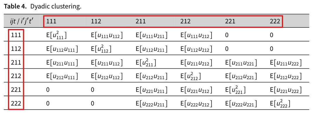
  • Proved AronowAudit.P032.toy_shared_country_covariance Historical support retained; baseline fidelity: ok; manifest: used; used in Solution; T12(ii) expressly permits pairwise uncorrelatedness of all five primitives, so using it in place of mutual independence excludes none of the specified target cases. In particular the two shocks are required to have zero covariance. If the quoted prose were read as only independence between the X and U families, a shock-covariance term would remain; that alternative is not the explicit formal reading supplied in the target.
  • Proved AronowAudit.P032.toy_sign_cases Historical support retained; baseline fidelity: ok; manifest: used; used in Solution; The positive shared-factor variance antecedent is in T12(iii) itself, so it is not a restriction disclosed only in the row description. The zero-variance case is explicitly covered by equality. The target name says as printed, whereas the earlier record calls T12 corrected: the formal clauses disambiguate the printed independence wording and qualify the printed strict sign sentence; this wording inconsistency does not alter the supplied mathematical target.

Introduction (p. 187), Section 3 (p. 191) and Conclusion (p. 196): the claim that with dependence between non-incident dyads ‘DCRSEs will still underestimate uncertainty’, so that the reanalysis ‘offers a lower bound’. Exact positive-definite error covariances, in bounded exogenous models, for which the dyadic restriction overstates the variance of a coefficient, and for which the residual-based DCR estimator overstates it in expectation and in the limit (the validators’ constructions; not in the paper)

p. 187 (PDF p. 2), paragraph beginning ‘Note, however’; p. 191 (PDF p. 6), paragraph beginning ‘Note that the above approach’; p. 196 (PDF p. 11), Conclusion, first and third paragraphs

pp. 187, 191 and 196, validator counterexamples (a)–(f). The bounded pair, four-record and six-edge models give the stated population comparisons, finite residual-estimator expectations, independent realizations and probability limits.

Historical component credits
  • Proved AronowAudit.P032.pair_error_moments Historical support retained; baseline fidelity: ok; manifest: used; used in Solution; Role: bounded pair-law mean and covariance certificates for T1(a)–(c). Because X is fixed, these zero means give the stated exogeneity; raw second moments equal covariance.
  • Proved AronowAudit.P032.pair_omega_positive_definite Historical support retained; baseline fidelity: ok; manifest: used; used in Solution; Supporting calculation or transfer lemma already incorporated in the selected complete model, finite-replication or limit declarations; not separately invoked.
  • Counterexample proved AronowAudit.P032.intercept_counterexample Historical support retained; baseline fidelity: ok; manifest: used; used in Solution; Role: the population numerical witness of T1(a), with centering and covariance realization in R205-10 and positivity in R205-09/R205-11. Its conclusion is about the population covariance restriction; the residual-estimator and asymptotic assertions belong to other rows. No claim-stage verdict changed.
  • Counterexample proved AronowAudit.P032.slope_and_sign_control Historical support retained; baseline fidelity: ok; manifest: used; used in Solution; This row supplies the numerical and slope-OLS portion of T1(b)–(c), not a full logical negation of the printed assertion. The explicit bounded centered law above verifies that its witness satisfies the model hypotheses; companion declarations separately export these facts.
  • Proved AronowAudit.P032.four_block_moments Historical support retained; baseline fidelity: ok; manifest: used; used in Solution; Auxiliary moment certificate for the specified witness; with fixed X, mean zero is the required exogeneity condition.
  • Proved AronowAudit.P032.four_omega_square_certificate Historical support retained; baseline fidelity: ok; manifest: used; used in Solution; Supporting calculation or transfer lemma already incorporated in the selected complete model, finite-replication or limit declarations; not separately invoked.
  • Counterexample proved AronowAudit.P032.four_block_counterexample Historical support retained; baseline fidelity: ok; manifest: used; used in Solution; This is the numerical population-witness component of T1(d), not an attempted standalone refutation of every possible estimator reading. The same explicit model satisfies boundedness, exogeneity and full rank; centering and positive definiteness are also established by the other local rows.
  • Proved AronowAudit.P032.six_block_variances Historical support retained; baseline fidelity: ok; manifest: used; used in Solution; Role: the six-edge population row sums and scalar variance values of T1(f); realizing moments, spectrum and replicated-estimator limits are assigned elsewhere. No claim-stage verdict changed.
  • Proved AronowAudit.P032.six_omega_square_certificate Historical support retained; baseline fidelity: ok; manifest: used; used in Solution; Supporting calculation or transfer lemma already incorporated in the selected complete model, finite-replication or limit declarations; not separately invoked.
  • Proved AronowAudit.P032.intercept_dcr_centering Historical support retained; baseline fidelity: ok; manifest: used; used in Solution; Supporting calculation or transfer lemma already incorporated in the selected complete model, finite-replication or limit declarations; not separately invoked.
  • Counterexample proved AronowAudit.P032.four_residual_expectation_counterexample Historical support retained; baseline fidelity: ok; manifest: not used; not used in Solution; Supporting calculation or transfer lemma already incorporated in the selected complete model, finite-replication or limit declarations; not separately invoked.
  • Proved AronowAudit.P032.four_expected_gap_arithmetic Historical support retained; baseline fidelity: ok; manifest: used; used in Solution; Supporting calculation or transfer lemma already incorporated in the selected complete model, finite-replication or limit declarations; not separately invoked.
  • Proved AronowAudit.P032.six_expected_gap_arithmetic Historical support retained; baseline fidelity: ok; manifest: used; used in Solution; Supporting calculation or transfer lemma already incorporated in the selected complete model, finite-replication or limit declarations; not separately invoked.
  • Proved AronowAudit.P032.finite_law_probability Historical support retained; baseline fidelity: ok; manifest: used; used in Solution; Supporting calculation or transfer lemma already incorporated in the selected complete model, finite-replication or limit declarations; not separately invoked.
  • Proved AronowAudit.P032.finite_law_integral Historical support retained; baseline fidelity: ok; manifest: used; used in Solution; Supporting calculation or transfer lemma already incorporated in the selected complete model, finite-replication or limit declarations; not separately invoked.
  • Proved AronowAudit.P032.finite_law_variance Historical support retained; baseline fidelity: ok; manifest: used; used in Solution; Supporting calculation or transfer lemma already incorporated in the selected complete model, finite-replication or limit declarations; not separately invoked.
  • Proved AronowAudit.P032.intercept_fit_certificate Historical support retained; baseline fidelity: ok; manifest: used; used in Solution; Role: OLS-to-explicit-estimator auxiliary. The nonempty-sample premise follows from m≥1 and n=4m or 6m in the target; it also prevents the singular-inverse convention.
  • Proved AronowAudit.P032.block_eigenbasis_certificates Historical support retained; baseline fidelity: ok; manifest: used; used in Solution; The invertible finite-dimensional eigenbasis identities entail both the listed eigenvalues and their complete multiplicities; the row is explicitly scoped to this spectral component.
  • Proved AronowAudit.P032.sum_squares_positive Historical support retained; baseline fidelity: ok; manifest: used; used in Solution; Supporting calculation or transfer lemma already incorporated in the selected complete model, finite-replication or limit declarations; not separately invoked.
  • Proved AronowAudit.P032.block_covariances_positive_definite Historical support retained; baseline fidelity: ok; manifest: used; used in Solution; Auxiliary positive-definiteness certificates for T1(d),(f), with no covariance-positivity premise.
  • Counterexample proved AronowAudit.P032.bounded_pair_sampling_models Historical support retained; baseline fidelity: ok; manifest: used; used in Solution; This row validates the bounded pair models and their actual OLS variances. Zero means/covariance realization and the dyadic comparison are separately credited components, explicitly identified by row_says; this is not a standalone full refutation or a claim about residual-based variance.
  • Proved AronowAudit.P032.lifted_intersection Historical support retained; baseline fidelity: ok; manifest: used; used in Solution; Supporting calculation or transfer lemma already incorporated in the selected complete model, finite-replication or limit declarations; not separately invoked.
  • Proved AronowAudit.P032.replicated_pattern Historical support retained; baseline fidelity: ok; manifest: used; used in Solution; Supporting calculation or transfer lemma already incorporated in the selected complete model, finite-replication or limit declarations; not separately invoked.
  • Proved AronowAudit.P032.replicated_row_sum Historical support retained; baseline fidelity: ok; manifest: used; used in Solution; Supporting calculation or transfer lemma already incorporated in the selected complete model, finite-replication or limit declarations; not separately invoked.
  • Proved AronowAudit.P032.replicated_quadratic Historical support retained; baseline fidelity: ok; manifest: used; used in Solution; Supporting calculation or transfer lemma already incorporated in the selected complete model, finite-replication or limit declarations; not separately invoked.
  • Proved AronowAudit.P032.four_replicated_centering Historical support retained; baseline fidelity: ok; manifest: used; used in Solution; Supporting calculation or transfer lemma already incorporated in the selected complete model, finite-replication or limit declarations; not separately invoked.
  • Proved AronowAudit.P032.six_replicated_centering Historical support retained; baseline fidelity: ok; manifest: used; used in Solution; Supporting calculation or transfer lemma already incorporated in the selected complete model, finite-replication or limit declarations; not separately invoked.
  • Proved AronowAudit.P032.finite_law_map Historical support retained; baseline fidelity: ok; manifest: used; used in Solution; Supporting calculation or transfer lemma already incorporated in the selected complete model, finite-replication or limit declarations; not separately invoked.
  • Proved AronowAudit.P032.finite_law_composed_integral Historical support retained; baseline fidelity: ok; manifest: used; used in Solution; Supporting calculation or transfer lemma already incorporated in the selected complete model, finite-replication or limit declarations; not separately invoked.
  • Proved AronowAudit.P032.pair_eigenbasis_certificate Historical support retained; baseline fidelity: ok; manifest: used; used in Solution; Role: the complete spectral certificate for T1(a),(b). The inverse identity exports basis completeness as well as the eigenvector equations; a separate sampling conclusion is not part of this row’s assigned component. No claim-stage verdict changed.
  • Proved AronowAudit.P032.four_block_statistics Historical support retained; baseline fidelity: ok; manifest: used; used in Solution; Supporting calculation or transfer lemma already incorporated in the selected complete model, finite-replication or limit declarations; not separately invoked.
  • Proved AronowAudit.P032.finite_law_identDistrib Historical support retained; baseline fidelity: ok; manifest: used; used in Solution; Supporting calculation or transfer lemma already incorporated in the selected complete model, finite-replication or limit declarations; not separately invoked.
  • Proved AronowAudit.P032.finite_law_composed_memLp Historical support retained; baseline fidelity: ok; manifest: used; used in Solution; Supporting calculation or transfer lemma already incorporated in the selected complete model, finite-replication or limit declarations; not separately invoked.
  • Proved AronowAudit.P032.iid_finite_statistic_variance Historical support retained; baseline fidelity: ok; manifest: used; used in Solution; Supporting calculation or transfer lemma already incorporated in the selected complete model, finite-replication or limit declarations; not separately invoked.
  • Proved AronowAudit.P032.iid_finite_statistic_integral Historical support retained; baseline fidelity: ok; manifest: used; used in Solution; Supporting calculation or transfer lemma already incorporated in the selected complete model, finite-replication or limit declarations; not separately invoked.
  • Proved AronowAudit.P032.four_replicated_moments Historical support retained; baseline fidelity: ok; manifest: used; used in Solution; Supporting calculation or transfer lemma already incorporated in the selected complete model, finite-replication or limit declarations; not separately invoked.
  • Proved AronowAudit.P032.four_replicated_finite Historical support retained; baseline fidelity: ok; manifest: used; used in Solution; The infinite-coordinate representation loses no finite iid block law: its first m blocks have exactly the prescribed m-fold product law, and any m independent copies yield that same joint distribution. The fixed-design intercept fit is the sample mean, and no error moment, expectation gap or limit is assumed.
  • Proved AronowAudit.P032.iid_finite_statistic_strong_law Historical support retained; baseline fidelity: ok; manifest: used; used in Solution; Supporting calculation or transfer lemma already incorporated in the selected complete model, finite-replication or limit declarations; not separately invoked.
  • Proved AronowAudit.P032.four_replicated_ratio_formula Historical support retained; baseline fidelity: ok; manifest: used; used in Solution; Supporting calculation or transfer lemma already incorporated in the selected complete model, finite-replication or limit declarations; not separately invoked.
  • Proved AronowAudit.P032.four_replicated_ratio_ae Historical support retained; baseline fidelity: ok; manifest: used; used in Solution; Supporting calculation or transfer lemma already incorporated in the selected complete model, finite-replication or limit declarations; not separately invoked.
  • Proved AronowAudit.P032.four_replicated_limit Historical support retained; baseline fidelity: ok; manifest: used; used in Solution; Convergence in mu-measure is convergence in probability because mu is explicitly a probability measure. The zero-size term totalizes to zero but all positive-size denominators are nonzero; target metadata incorrectly says asymptotic=false despite explicitly requesting this limit.
  • Proved AronowAudit.P032.finite_law_atom Historical support retained; baseline fidelity: ok; manifest: used; used in Solution; Supporting calculation or transfer lemma already incorporated in the selected complete model, finite-replication or limit declarations; not separately invoked.
  • Proved AronowAudit.P032.six_sign_measure_product Historical support retained; baseline fidelity: ok; manifest: used; used in Solution; Equality is of actual probability measures, with no independence or moment assumption hidden in a structure field.
  • Proved AronowAudit.P032.fair_sign_moments Historical support retained; baseline fidelity: ok; manifest: used; used in Solution; Supporting calculation or transfer lemma already incorporated in the selected complete model, finite-replication or limit declarations; not separately invoked.
  • Proved AronowAudit.P032.six_loading_identity Historical support retained; baseline fidelity: ok; manifest: used; used in Solution; Supporting calculation or transfer lemma already incorporated in the selected complete model, finite-replication or limit declarations; not separately invoked.
  • Proved AronowAudit.P032.linear_covariance_identity Historical support retained; baseline fidelity: ok; manifest: used; used in Solution; Supporting calculation or transfer lemma already incorporated in the selected complete model, finite-replication or limit declarations; not separately invoked.
  • Proved AronowAudit.P032.six_loading_gram_certificate Historical support retained; baseline fidelity: ok; manifest: used; used in Solution; Supporting calculation or transfer lemma already incorporated in the selected complete model, finite-replication or limit declarations; not separately invoked.
  • Proved AronowAudit.P032.six_sign_error_moments Historical support retained; baseline fidelity: ok; manifest: used; used in Solution; Finite-law expectations compute the required moments, and the independently identified product law supplies the target’s thirteen independent fair signs.
  • Proved AronowAudit.P032.finite_expectation_sum Historical support retained; baseline fidelity: ok; manifest: used; used in Solution; Supporting calculation or transfer lemma already incorporated in the selected complete model, finite-replication or limit declarations; not separately invoked.
  • Proved AronowAudit.P032.finite_expectation_quadratic Historical support retained; baseline fidelity: ok; manifest: used; used in Solution; Supporting calculation or transfer lemma already incorporated in the selected complete model, finite-replication or limit declarations; not separately invoked.
  • Proved AronowAudit.P032.six_sign_statistics Historical support retained; baseline fidelity: ok; manifest: used; used in Solution; Supporting calculation or transfer lemma already incorporated in the selected complete model, finite-replication or limit declarations; not separately invoked.
  • Proved AronowAudit.P032.six_errors_bounded Historical support retained; baseline fidelity: ok; manifest: used; used in Solution; Role: boundedness auxiliary for the precise six-edge sign construction of T1(f). This is an everywhere statement on all 2^13 sign configurations, stronger than merely an a.e. bound under the fair law.
  • Proved AronowAudit.P032.iid_block_covariance Historical support retained; baseline fidelity: ok; manifest: used; used in Solution; Supporting calculation or transfer lemma already incorporated in the selected complete model, finite-replication or limit declarations; not separately invoked.
  • Proved AronowAudit.P032.block_matrix_quadratic Historical support retained; baseline fidelity: ok; manifest: used; used in Solution; Supporting calculation or transfer lemma already incorporated in the selected complete model, finite-replication or limit declarations; not separately invoked.
  • Proved AronowAudit.P032.block_matrix_restriction Historical support retained; baseline fidelity: ok; manifest: used; used in Solution; Supporting calculation or transfer lemma already incorporated in the selected complete model, finite-replication or limit declarations; not separately invoked.
  • Proved AronowAudit.P032.block_matrix_record_restriction Historical support retained; baseline fidelity: ok; manifest: used; used in Solution; Supporting calculation or transfer lemma already incorporated in the selected complete model, finite-replication or limit declarations; not separately invoked.
  • Proved AronowAudit.P032.constant_quadratic Historical support retained; baseline fidelity: ok; manifest: used; used in Solution; Supporting calculation or transfer lemma already incorporated in the selected complete model, finite-replication or limit declarations; not separately invoked.
  • Proved AronowAudit.P032.six_replicated_population_values Historical support retained; baseline fidelity: ok; manifest: used; used in Solution; Supporting calculation or transfer lemma already incorporated in the selected complete model, finite-replication or limit declarations; not separately invoked.
  • Proved AronowAudit.P032.six_replicated_moments Historical support retained; baseline fidelity: ok; manifest: used; used in Solution; Finite iid models are represented by prefixes of an infinite iid realization. Every allowed finite joint law is the same product law, so this representation loses no case of the distributional variance and expectation assertions.
  • Proved AronowAudit.P032.six_scaled_estimator_formula Historical support retained; baseline fidelity: ok; manifest: used; used in Solution; Supporting calculation or transfer lemma already incorporated in the selected complete model, finite-replication or limit declarations; not separately invoked.
  • Proved AronowAudit.P032.six_replicated_finite Historical support retained; baseline fidelity: ok; manifest: used; used in Solution; The infinite iid sequence is a representation of the fixed finite product laws used by the counterexample, not an exclusion of any allowed finite law: each statistic depends only on the first m blocks, and all finite realizations have the same distribution. The statement includes all nine described conclusions; its uncentered errorCovariance is a covariance because zero means are proved.
  • Proved AronowAudit.P032.six_replicated_limit Historical support retained; baseline fidelity: ok; manifest: used; used in Solution; Target metadata inconsistency: asymptotic=false although T1(f) explicitly includes this almost-sure limit (and T1(e) includes another limit). The Lean conclusion matches the target text.
  • Proved AronowAudit.P032.finite_law_iid_exists Historical support retained; baseline fidelity: ok; manifest: used; used in Solution; Auxiliary iid realization supporting T1(e),(f). The T5 prefix in row_says is a cross-reference to the printed lower-bound refutation using the same realization, not a different mathematical assertion.

Introduction (p. 187), Section 3 (p. 191) and Conclusion (p. 196), as printed: with dependence between non-incident dyads ‘DCRSEs will still underestimate uncertainty’, and the reanalysis ‘offers a lower bound’

p. 187 (PDF p. 2), paragraph beginning ‘Note, however’; p. 191 (PDF p. 6), paragraph beginning ‘Note that the above approach’; p. 196 (PDF p. 11), Conclusion, first and third paragraphs

pp. 187, 191 and 196, formal universal lower-bound readings. The validators' unrestricted weak and strict population, residual-estimator expectation, and relative probability-limit readings of the quoted passages all fail, establishing the canonical assertion that those four readings are false.

Historical component credits
  • Counterexample proved AronowAudit.P032.printed_population_claim_false Historical support retained; baseline fidelity: ok; manifest: used; used in Solution; A finite PSD matrix is an admissible covariance in the target setting; this particular countermodel has an explicit bounded centered law. Both weak and strict printed universal orderings fail in that same model.
  • Counterexample proved AronowAudit.P032.printed_expectation_claim_false Historical support retained; baseline fidelity: ok; manifest: used; used in Solution; The expectation is of the residual-based variance estimator, as in T5’s formal reading, rather than the expectation of its square root. The universal proposition is fully expanded and contains no assumed lower-bound conclusion.
  • Counterexample proved AronowAudit.P032.printed_ratio_limit_claim_false Historical support retained; baseline fidelity: ok; manifest: used; used in Solution; {'source': 'adjudication', 'decision': 'rejected', 'what': 'P032/P032_Dyadic.lean:3192 refutes PrintedRatioLimitLowerBound, whose definition at line 1960 compares the actual dyadic residual plug-in contrast with the actual OLS sampling variance. Its eventual-positive-variance and finite-probability-limit conditions at lines 1972 and 1974 cause no material mismatch for a counterexample: the bounded centered iid four-observation-block model has positive sampling variance 3/[16(m+1)] and ratio limit 5/3, contradicting the universal limiting underestimation reading included in T5. Refuting that reading does not require universal existence of a ratio limit, and the growing finite record types merely relabel sample sizes. The only correction needed is descriptive: T5 includes a limit claim despite asymptotic=false and S7 saying every target is an exact finite statement.'}

The decomposition display (p. 191) as implemented by the Stata command for survival data that are stset with an id() variable (Efrat and Newman 2016; Weisiger 2016): exact Cox example in which subtracting (N−2)(N-2) times the id-clustered matrix in place of (N−2)V^0(N-2)\hat V_0 does not give the DCR estimator (the validators’ construction; not in the paper)

p. 191 (PDF p. 6), display for V^r\hat V_r and the definition of V^0\hat V_0; dcr.ado lines 163–190; code/1_reanalysis_stata.do lines 319–334 and 347–418; Supplementary Table A.2 (supplement p. A3), rows Efrat and Newman (2016) and Weisiger (2016)

p. 191 decomposition; dcr.ado lines 108–119 and 163–190, constructed example. The specified Cox fit has the stated risk sets, scores and component covariances, and the two subject-id substitutions give the stated incorrect positive values.

Historical component credits
  • Proved AronowAudit.P032.cox_risk_score_certificate Historical support retained; baseline fidelity: ok; manifest: used; used in Solution; Auxiliary witness certificate for T3(a,b); the exact risk sets themselves are exported by R208-02, and the fit by R208-07. The information is the explicit Breslow risk-variance expression at zero, not an assumed desired value.
  • Proved AronowAudit.P032.cox_unique_fit Historical support retained; baseline fidelity: ok; manifest: used; used in Solution; The record assigns faithful_with_notes for validator-origin data, zero-based indexing, censoring and Breslow conventions. These conventions were already checked in the blind translation and coincide with T3's own model, so the saved faithful verdict is unchanged.
  • Proved AronowAudit.P032.cox_components Historical support retained; baseline fidelity: ok; manifest: used; used in Solution; Auxiliary witness certificate for T3(c); equality of id and repeated-dyad partitions is exported separately by R208-03. The score vector and information bread are linked to the fitted model by R208-04 and R208-07.
  • Counterexample proved AronowAudit.P032.cox_substitution_counterexample Historical support retained; baseline fidelity: ok; manifest: used; used in Solution; Exact witness for the specified id-substitution error, not a negation of the valid printed decomposition. The non-direct component formulas use rational constants whose identification with actual fitted components is supplied by R208-01 through R208-05 and R208-07; all three positive scalar outputs are unchanged by eigenvalue clipping. No assertion about executing Stata or about the affected studies' numerical results is made.
  • Proved AronowAudit.P032.cox_exact_risk_sets Historical support retained; baseline fidelity: ok; manifest: used; used in Solution; Auxiliary witness certificate for T3(a); zero-based labels are a bijective reindexing of the exact target data.
  • Proved AronowAudit.P032.cox_subject_score_totals Historical support retained; baseline fidelity: ok; manifest: used; used in Solution; Auxiliary witness certificate for T3(b); these are the efficient scores before multiplication by the common bread 1/12.
  • Proved AronowAudit.P032.cox_id_is_repeated_dyad Historical support retained; baseline fidelity: ok; manifest: used; used in Solution; Auxiliary witness certificate for the constructed dataset only; it asserts no equivalence of subject and dyad partitions for other survival samples.

The positive-semidefinite option of the released software (posdef in R, psd in Stata), documented as forcing the DCR variance matrix to be positive semidefinite, and footnote 3 (p. 191): exact ten-dyad least-squares sample whose DCR matrix has a positive diagonal and a negative eigenvalue, so that the option returns it unchanged (the validator’s construction; not in the paper)

p. 191 (PDF p. 6), footnote 3; R package dcr, R/dyad_funcs.R lines 70 and 155, man/dcr.Rd and man/dcr_sandwich.Rd (argument posdef); dcr.ado lines 246–281 and dcr.hlp line 86 (option psd)

p. 191 footnote 3 and the released PSD option, validator ten-dyad example. The specified OLS covariance has a positive diagonal and a negative contrast, so the diagonal gate leaves a matrix that is not positive semidefinite.

Historical component credits
  • Proved AronowAudit.P032.ten_ols_certificate Historical support retained; baseline fidelity: ok; manifest: used; used in Solution; Auxiliary witness certificate for T6(a); the inverse relation and explicit nonsingular Gram matrix establish full rank without assuming it.
  • Proved AronowAudit.P032.ten_variance_certificate Historical support retained; baseline fidelity: ok; manifest: used; used in Solution; Auxiliary witness certificate for T6(b,c); the score definition is fitted residual times the two design coordinates, and V uses the actual OLS bread by R208-17.
  • Counterexample proved AronowAudit.P032.positive_diagonal_counterexample Historical support retained; baseline fidelity: ok; manifest: used; used in Solution; Exact witness against the documented diagonal-gated PSD guarantee, not against the correct unconditional eigenvalue-clipping operation. The universal gate clause over symmetry proofs is inhabited by R208-19; R208-17 and R208-18 tie this matrix to the actual full-rank OLS fit.
  • Proved AronowAudit.P032.ten_variance_hermitian Historical support retained; baseline fidelity: ok; manifest: used; used in Solution; Auxiliary witness certificate for T6(d) and the symmetry premise of its spectral operations; real Hermitian means exactly symmetric.
  • Proved AronowAudit.P032.ten_meat_decomposition Historical support retained; baseline fidelity: ok; manifest: used; used in Solution; Auxiliary T6(b) meat identity: all ten unordered dyads are distinct in the enumerated input, and H is the record-pattern meat. This is an identity before multiplying by the bread.

The DCR variance under multiple imputation, corrected: finite-sample factors removed within each completed data set, DCR formed within each, and Rubin’s between-imputation term added once; with the exact gap of the pooled-first procedure

Code only (no passage of main.pdf): code/1_reanalysis_stata.do lines 1373–1385; dcr.ado lines 125–238. The decomposition used is the display on p. 191 (PDF p. 6)

code/1_reanalysis_stata.do lines 1373–1385; dcr.ado lines 125–238; p. 191 (PDF p. 6), decomposition display. For at least two imputations, common coefficient estimates, fixed nonzero component factors and symmetric completed-data matrices, with no active PSD adjustment, the pooled-first total is the weighted within-imputation mean plus c times Rubin's full between-imputation term Q = (1 + 1/M)B. Combining within each imputation and then pooling gives the same within mean plus Q, so the gap is (c - 1)Q and adding (1 - c)Q repairs it. The DCR weights sum to one and, when all factors are one, decomposition commutes with Rubin pooling. For the asylike factors, c - 1 = -sum_i 1/G_i + 1/G_D + (K - 2)/n; at K = 4, G_i = 13, G_D = 6, n = 24 it is -3/52 and is nonzero. The standalone scalar identity also holds for zero denominators under Lean's total division.

Historical component credits
  • Proved AronowAudit.P032.rubin_pooling_gap Historical support retained; baseline fidelity: ok; manifest: used; used in Solution; The imputation-count and symmetry assumptions are present in the target, even though the equalities do not mathematically need them. Common estimates and fixed factors are encoded by shared function inputs; changing samples, factors or active PSD operations is outside this target setting.
  • Proved AronowAudit.P032.dcr_weights_sum Historical support retained; baseline fidelity: ok; manifest: used; used in Solution; Auxiliary scalar weight identity; the commutation consequence uses R209-20. k-2 is subtraction in the reals, so k=0 or 1 does not introduce natural-number truncation.
  • Proved AronowAudit.P032.asylike_coefficient_gap Historical support retained; baseline fidelity: ok; manifest: used; used in Solution; Auxiliary scalar identity; zero reciprocal cases are only additional valid algebraic cases. The admissible counts of T8 give a nonzero instance, while R209-19 supplies the matrix-gap interpretation with its stated hypotheses.
  • Proved AronowAudit.P032.rubin_unadjusted_commutes Historical support retained; baseline fidelity: ok; manifest: used; used in Solution; This is the abstract commutation component, combined with the DCR weight certificate R209-18. The imputation-count and symmetry assumptions match the target and do not narrow it.

The Schneider and Tobin (2020) calls of the replication code (dcr with the prefix ‘mi estimate, post:’ and dofundo(asylike)): exact five-imputation, 24-observation intercept-only logit example in which removing the finite-sample factors from Rubin-pooled matrices does not give the Rubin-pooled DCR variance (the validator’s construction; not in the paper)

Code only (no passage of main.pdf): code/1_reanalysis_stata.do lines 1312 and 1373–1385; dcr.ado lines 125–238; the results enter Supplementary Table A.2 (supplement p. A3), row Schneider and Tobin (2020). The decomposition used is the display on p. 191 (PDF p. 6)

1_reanalysis_stata.do lines 1312 and 1373–1385; dcr.ado lines 125–238. The specified five-imputation logit example has the stated fits, components and strictly negative pooled-first discrepancy, with scalar clipping inactive. Restricted: the separate equalities of the two completed-data decomposition values with direct ordered-pair sums are not asserted.

Historical component credits
  • Proved AronowAudit.P032.mi_completed_data_certificate Historical support retained; baseline fidelity: ok; manifest: used; used in Solution; Auxiliary certificates for T8(a)-(c). The target definitions explicitly supply the intercept-only logit fit formulas, so a separate likelihood maximization theorem is unnecessary; the component combination is the DCR variance by the decomposition specified in definitions_needed.
  • Proved AronowAudit.P032.mi_between_certificate Historical support retained; baseline fidelity: ok; manifest: used; used in Solution; Auxiliary certificate for the concrete witness, not a positive general claim about MI or a full refutation. The supplied target definitions specify exactly this Rubin mean, B and Q.
  • Counterexample proved AronowAudit.P032.mi_pooling_counterexample Historical support retained; baseline fidelity: ok; manifest: used; used in Solution; Exact witness for the pooled-first versus within-imputation discrepancy specified by T8. This does not purport to run Stata, identify numerical errors in the empirical study, or refute a positive assertion in the article; the target is explicitly code-only. R209-14 supplies positive completed-data DCR values.
  • Proved AronowAudit.P032.mi_partition_counts Historical support retained; baseline fidelity: ok; manifest: used; used in Solution; Auxiliary partition-count certificate. The outsider singleton convention is the one explicitly stated in T8(b), and 24-12=12 gives the remaining singleton count and hence 13 clusters.

Section 4.1 (p. 196), ‘Three studies see half or more of their KEVs become insignificant at the 5% level upon reanalysis’, corrected against Supplementary Table A.2: four studies have a Sig.→Insig. share of one half or more, and three have a share above one half

p. 196 (PDF p. 11), Section 4.1, paragraph beginning ‘For individual studies’; Supplementary Table A.2 (supplement p. A3), columns KEVs, Sig.→Insig. and Avg. SER

p. 196 Section 4.1 and Supplementary Table A.2, p. A3. Exact recovery from the printed proportions gives four studies at the weak half-loss threshold and three at the strict threshold, together with all stated neighboring counts.

Historical component credits
  • Proved AronowAudit.P032.study_unique_integer_recovery Historical support retained; baseline fidelity: ok; manifest: used; used in Solution; The rational-recovery declaration already incorporates this integer-rounding step; not separately invoked.
  • Proved AronowAudit.P032.study_threshold_counts Historical support retained; baseline fidelity: ok; manifest: used; used in Solution; The row proves the corrected count, rather than the false printed count of three at the weak threshold. The fixed table and numerator-recovery rows identify the four studies; the strict threshold correctly excludes the 2/4 case.
  • Proved AronowAudit.P032.study_neighboring_counts Historical support retained; baseline fidelity: ok; manifest: used; used in Solution; T10(iv) is explicitly arithmetic on the printed table. The n and SER entries match the target exactly; thousandths encode its finite decimals without approximation. This is not empirical validation of the underlying estimates.
  • Proved AronowAudit.P032.rounding_consistent_iff_rational Historical support retained; baseline fidelity: ok; manifest: used; used in Solution; The rational-recovery declaration already incorporates this integer-rounding step; not separately invoked.
  • Proved AronowAudit.P032.study_unique_rational_recovery Historical support retained; baseline fidelity: ok; manifest: used; used in Solution; The tolerance is closed at both endpoints exactly as in T10(i); none of the target rows is ambiguous. The statement certifies the printed-table arithmetic, rather than a rerun of significance tests.

Reproduction

What I recalculated or reran from public materials. "Agrees", "Agrees in part" or "Disagrees" compares my result with the printed one. "Not compared" means the comparison could not be made.

Status
Partial reproduction
Agreement
Agrees in part
Reported results that were targeted
TargetWhereMethodStatusAgreement
Table 5 and analytic samplep. 193 (PDF p. 8), sample description p. 192 (PDF p. 7)I recalculated all 77 printed Table 5 cells from saved study summaries, using the two R-study rows as printed. This reproduces the sample selected by the original merge; P032-E008 identifies two omitted KEVs and gives the corrected counts.RecalculatedAgrees in part
Figure 1p. 194 (PDF p. 9), upper panelI visually compared the published figure with the saved full-data figure in the replication files; they agree. Complete regeneration was blocked because five KEVs from one model were unavailable. Newly generated figures omit those KEVs and do not establish complete-data agreement.BlockedAgrees
Figure 2p. 194 (PDF p. 9), lower panelI visually compared the published figure with the saved full-data figure in the replication files; they agree. Complete regeneration was blocked because five KEVs from one model were unavailable. Newly generated figures omit those KEVs and do not establish complete-data agreement.BlockedAgrees
Figure 3p. 195 (PDF p. 10)I visually compared the published figure with the saved full-data figure in the replication files; they agree. Complete regeneration was blocked because five KEVs from one model were unavailable. Newly generated figures omit those KEVs and do not establish complete-data agreement.BlockedAgrees
Abstract significance retentionp. 186 (PDF p. 1), abstract; p. 196 (PDF p. 11), conclusionI recalculated retention using integer transition counts recovered from the printed study summaries, with equal study weighting: about 67.03%67.03\%, which rounds to the reported 67%67\%.RecalculatedTo rounding
Table A.2 and study-level in-text resultssupplement p. A3 (supplement PDF p. 3); main p. 196 (PDF p. 11)I compared 21 complete study rows from the partial replication merge with Table A.2; they agree to rounding, and the remaining study is incomplete. The reported range and the counts 18 and seven agree, but four studies, rather than the stated three, lose significance for at least half their KEVs (P032-E002).RecalculatedAgrees in part