LLM-generated corrections to the published research of P. M. Aronow

Journal article P018

Corrections to: Cluster-Robust Variance Estimation for Dyadic Data

P. M. Aronow, Cyrus Samii, and Valentina A. Assenova (2015). Cluster-Robust Variance Estimation for Dyadic Data. Political Analysis 23(4):564–577.

DOI
10.1093/pan/mpv018
arXiv
1312.3398
Audited edition
Political Analysis, 2015, 23(4):564–577; 14 pages in the audited file
SHA-256 of the audited file
2f17ede379ebb939a85604d8b02eb237c9c74dffdfd73b46ff0b3070153e9caf
Permanent address
https://pmaronow.github.io/llm-audit/works/P018/

Summary

The paper proposes a sandwich variance estimator for regression with dyadic data, where dyads that share a unit may be dependent. It states conditions for consistency as the number of units grows, and evaluates the estimator in simulations and a reanalysis of interstate disputes. 21 entries are classified as errors (4 Moderate, 17 Minor), and 2 are clarity notes; 2 other allegations were not confirmed and 4 lie outside the paper. The main finding is P018-E001: equation (2) expresses an unconditional variance using conditional residual variances and covariances, which can omit a variance contribution when the conditional mean is not linear. Correcting this formula leaves estimator (3) unchanged.

What was and was not checked

I checked the following points, with the corrections and qualifications noted below.

  • Lemma 1, equation (1), and the conclusion NV^−V→p0N\hat V-V\overset{p}{\to}0 of Proposition 1, with the variance of the score sum as corrected in P018-E001. The algebra of the OLS estimator and the orthogonality E[Xdϵd]=0\mathrm{E}[X_d\epsilon_d]=0 hold. Estimator (3) contains the product of each dyad with itself, and each ordered pair of distinct dyads that share a unit, exactly once. Dyads that share no unit contribute no covariance. Since NV^N\hat V estimates the variance of N(β^−β)\sqrt{N}(\hat\beta-\beta), the square roots of the diagonal of V^\hat V are on the scale of standard errors. The printed proof of Proposition 1 is the subject of P018-E006, and the claims about inference are the subject of P018-E002.
  • The counts used in the proofs are correct. There are 2D(N−2)2D(N-2) ordered pairs of distinct dyads that share a unit. This number is of order N3=O(D3/2)N^3=O(D^{3/2}), as Appendix A requires for the convergence of D−1∑dXdXd′D^{-1}\sum_dX_dX_d'. In Appendix B, two pairs of overlapping dyads that are dependent involve at most five distinct units. There are O(N5)O(N^5) such terms among O(N6)O(N^6), and I obtain the intended bound of order N−1N^{-1} when the residuals are the population residuals.
  • Proposition 2 and Appendix C: the identity V^r=∑iV^C,i−V^D−(N−2)V^0\hat V_r=\sum_i\hat V_{C,i}-\hat V_D-(N-2)\hat V_0 holds when each dyad that does not contain unit ii is counted once; the index is corrected in P018-E007. I counted how often each pair of observations appears on the two sides. On unbalanced repeated dyads with missing dyads, the two sides agree numerically to 5×10−155\times10^{-15}.
  • The R code of the authors computes estimator (3) and its repeated, weighted and logistic versions as the paper defines them. On the covariance matrix of the interstate application it agrees with a direct sum over units and dyads to 6.22×10−116.22\times10^{-11}. The correction of 2016 that is noted in the README of the replication files changes only the off-diagonal entries of V^\hat V. The diagonal entries, and with them every reported standard error, are the same before and after it.
  • Corollaries 1 and 2: the estimator V^r\hat V_r of Corollary 1 and the estimator V^w\hat V_w of equation (7) have the correct form, including the placement of the weights. The limits VrV_r and VwV_w are the subject of P018-E004, the conditions on the weights are the subject of P018-E003, and the first displays of the two corollaries are the subject of P018-N004.
  • Appendix E: the logistic score Xd(Yd−pd)X_d(Y_d-p_d) and the Hessian are correct, and the authors' code computes the estimator from them. The printed cross term is corrected in P018-E005, and the notation in P018-N010.
  • Section 4: the design as described agrees with the simulation script (500 runs; 20, 50, 100 and 150 units; β0=0\beta_0=0 and β1=1\beta_1=1; standard normal draws; two observations per dyad in the repeated case). The numbers of dyads, 190, 1,225, 4,950 and 11,175, are correct, and so is 10,585 for 146 states. I ran the simulations of Figure 1 and of Figures 2 and 3 of the Supporting Information again with 500 replications per cell. All 80 values read from the published figures agree with the new runs, within Monte Carlo error and the error of reading a figure. The true standard errors in Figure 1 agree with a first-order calculation, whose values are 0.551, 0.339, 0.237, 0.193 for β^0\hat\beta_0 and 0.280, 0.164, 0.113, 0.091 for β^1\hat\beta_1. Negative variance estimates in small samples are the subject of P018-N003, and the comparison with random effects is the subject of P018-E008.
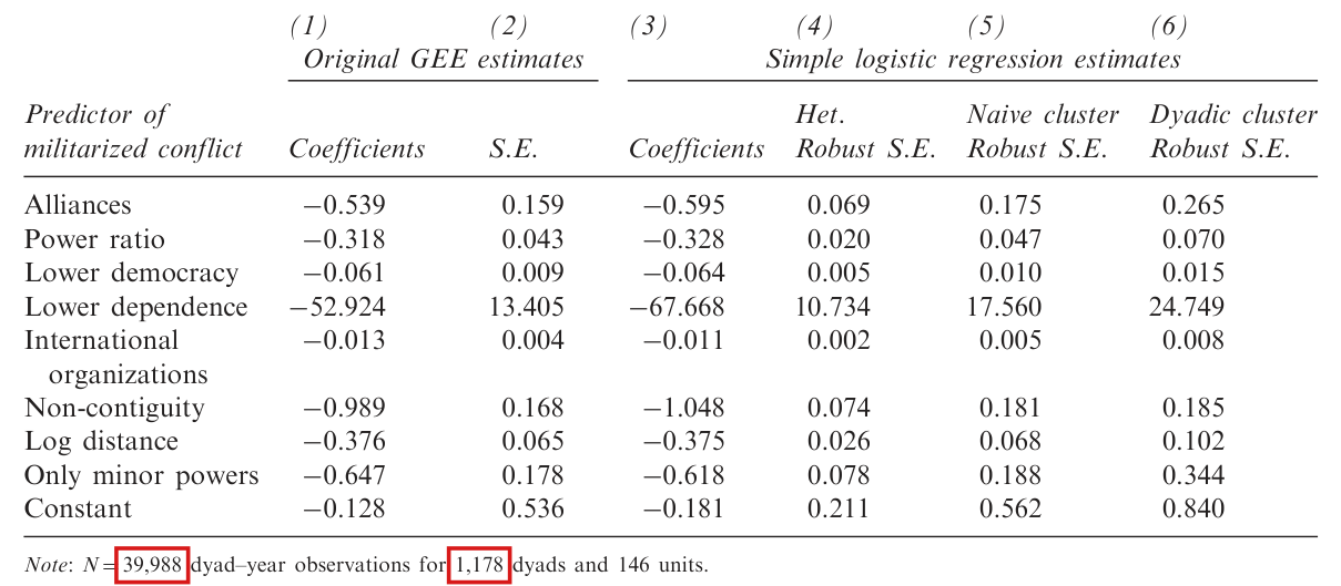
  • Table 1: all 36 entries of columns (3)–(6) are reproduced to the printed rounding from the data in the replication files. Column (4) agrees with the HC2 form of the heteroskedasticity-robust estimator, and column (5) agrees once a finite-sample factor is applied. I approximated the GEE columns (1) and (2) outside Stata, but did not reproduce every entry to the printed rounding. The coefficient for international organizations is −0.0112-0.0112 with dyadic-robust standard error 0.00850.0085, a ratio of −1.31-1.31, and every other slope exceeds 1.64 in absolute value. The sample counts are corrected in P018-E010, the description of this regressor in P018-E011, and the size of the ratios of standard errors in P018-E012.
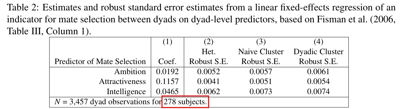
  • Table 2 of the Supporting Information: all 12 entries are reproduced to four decimals. The dyadic-robust standard errors exceed the heteroskedasticity-robust ones by 17% to 32% and those clustered on the woman by 1% to 7%, as the text says.

My checks had the following limits. The paper’s statements about Russett and Oneal (2001), Fisman et al. (2006), Lehmann (1999), Fafchamps and Gubert (2007) and Conley (1999) were not checked against those works. I consulted Hansen (2007) and Stock and Watson (2008) for the fixed-unit, growing-time remarks on p. 568. These sources do not support the implication that mixing makes the displayed variance estimator consistent for the normalized asymptotic covariance; see P018-N005. I did not confirm an error in the conclusion’s qualified expectation about higher-order dependence, or establish a general guarantee of underestimation or improvement. Stata was not available: the Stata script for Table 1 was not run, and the GEE columns were computed in other software. The replication files do not contain the output of the simulations, their seeds or the logs of the cluster jobs. The published simulation values were compared with values read from the figures, to within about 0.015, and not with the original draws. Figure 4 of the Supporting Information was not drawn again. The reports in Section 5 that the random-effects and spatial models produced no estimates after days of computation cannot be checked from the files. That this audit lists no further corrections is not a finding that the rest of the paper is correct.

Headline claims and related corrections

  1. The plug-in dyadic sandwich estimator V^\hat V in equation (3) consistently estimates the variance of the OLS coefficients as the number of units NN grows, when dependence is confined to dyads sharing a member: NV^−V→p0N\hat V-V\overset{p}{\to}0, with VV given by Lemma 1.

    Lemma 1 (eqs. 1-2); Proposition 1 (eq. 3); Appendices A-B

    See P018-E001, P018-E002, P018-E006, P018-N001, P018-N002, P018-N004.

  2. The estimator is robust to misspecification of the conditional mean: it gives asymptotically valid standard errors for the coefficients of the best linear approximation.

    Lemma 1; Proposition 1; footnote 2; SI Figure 3; Conclusion p. 572

    See P018-E001, P018-E002.

  3. The results extend to repeated observations (directed dyads, panels) and to weighted observations.

    Corollary 1 (V^r\hat V_r, VrV_r); Corollary 2 (equation (7), VwV_w); Appendix D

    See P018-E001, P018-E003, P018-E004, P018-N004, P018-N005.

  4. The variance estimator has a generalized-linear-model implementation, including logistic regression.

    Appendix E (V^l\hat V_l); Table 1

    See P018-E005, P018-N010.

  5. The dyadic estimator can be written as V^r=∑iV^C,i−V^D−(N−2)V^0\hat V_r=\sum_i\hat V_{C,i}-\hat V_D-(N-2)\hat V_0, a combination of ordinary cluster-robust and heteroskedasticity-robust estimators that can be computed with standard commands.

    Proposition 2; Appendix C; replication scripts 1, 5, 6

    See P018-E007.

  6. In the simulations, dyadic-robust standard errors approach the true standard errors and are reliable with roughly 50–100 units, while heteroskedasticity-robust and dyad-clustered standard errors substantially understate variability.

    Figure 1; SI Figures 2-3; replication scripts 1-3

    See P018-N003.

  7. A two-way random effects model is more efficient than OLS and has consistent standard errors when the conditional mean is correctly specified, but its standard errors are inconsistent and anti-conservative under mild misspecification, where the dyadic-robust standard errors remain valid.

    Section 4, pp. 569-570; SI Figures 2-4; Conclusion p. 572; replication scripts 1-3

    See P018-E008, P018-E009.

  8. In the Russett-Oneal reanalysis, dyadic-robust standard errors are much larger than heteroskedasticity-robust ones ('sometimes an order of magnitude') and considerably larger than dyad-clustered ones; the international-organizations coefficient is no longer significant at conventional levels.

    Table 1; Section 5, p. 571; replication scripts 4-5; TRIANGLE.dta

    See P018-E010, P018-E011, P018-E012, P018-E013.

  9. Random-effects and spatial error-lag models were computationally infeasible in the reported application, whereas the proposed variance estimator was easy to compute.

    p. 565; Section 5, p. 571; footnotes 6-7; Conclusion p. 572; Proposition 2

  10. In the speed-dating application (weighted, with female-subject fixed effects) dyadic-robust standard errors exceed heteroskedasticity-robust ones but differ little from standard errors clustered on the female subject, as expected given the limited dyadic dependence.

    Appendix D; SI Table 2; replication script 6

    See P018-E010.

Corrections

Moderate (4)

A real substantive error with limited reach.

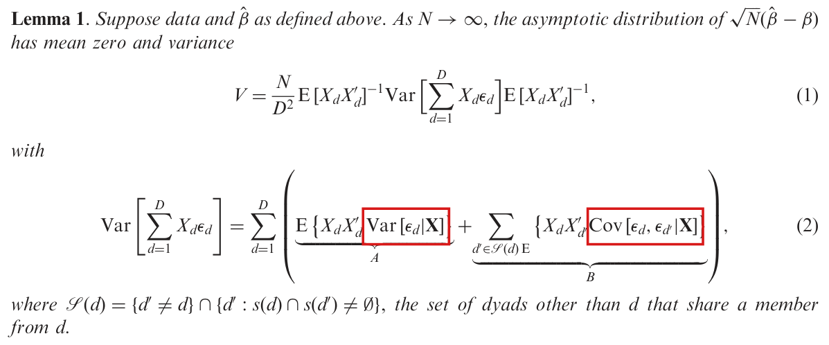
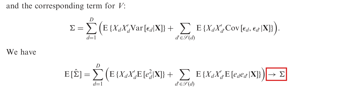
Equation (2) expresses the variance of the score sum through conditional variances and covariances of the residuals, which can omit Var⁡(E[∑dXdϵd∣X])\operatorname{Var}(\mathrm{E}[\sum_dX_d\epsilon_d\mid\mathbf{X}]) when the conditional mean is not linear; the terms should be the unconditional moments E{XdXd′ϵd2}\mathrm{E}\{X_dX_d'\epsilon_d^2\} and E{XdXd′′ϵdϵd′}\mathrm{E}\{X_dX_{d'}'\epsilon_d\epsilon_{d'}\}.

Lemma 1, equation (2), p. 566 (PDF p. 3); Appendix A, equation (6), second and third lines, p. 573 (PDF p. 10). The same form recurs in Σ\Sigma of Appendix B, p. 573, in VrV_r, p. 568 (PDF p. 5), and in VwV_w, p. 576 (PDF p. 13)

See also under Formal statements (Lean): P018-T1, P018-T2, P018-T21, P018-T26, P018-T27

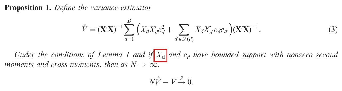
As printed

p. 566: “Lemma 1. Suppose data and β^\hat\beta as defined above. As N→∞N\to\infty, the asymptotic distribution of N(β^−β)\sqrt{N}(\hat\beta-\beta) has mean zero and variance

V=ND2 E[XdXd′]−1Var⁡[∑d=1DXdϵd]E[XdXd′]−1,(1)V=\frac{N}{D^2}\,\mathrm{E}[X_dX_d']^{-1}\operatorname{Var}\Big[\sum_{d=1}^{D}X_d\epsilon_d\Big]\mathrm{E}[X_dX_d']^{-1},\qquad(1)

with

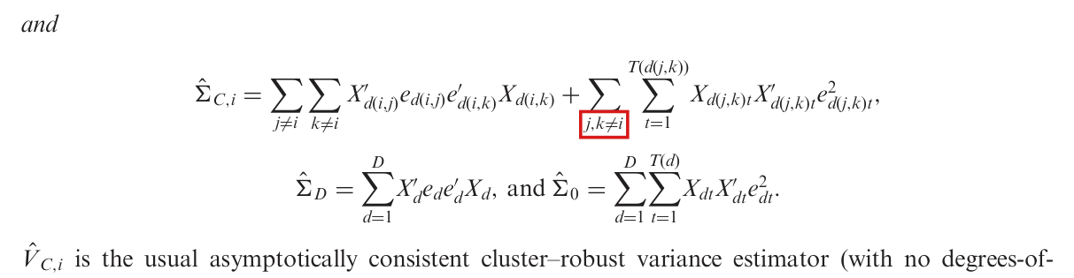
Var⁡[∑d=1DXdϵd]=∑d=1D(E{XdXd′Var⁡[ϵd∣X]}⏟A+∑d′∈S(d) E{XdXd′′Cov⁡[ϵd,ϵd′∣X]}⏟B),(2)\operatorname{Var}\Big[\sum_{d=1}^{D}X_d\epsilon_d\Big]=\sum_{d=1}^{D}\Big(\underbrace{\mathrm{E}\{X_dX_d'\colorbox{#ffe58a}{$\displaystyle \operatorname{Var}[\epsilon_d|\mathbf{X}]$}\}}_{A}+\underbrace{\sum_{d'\in\mathcal{S}(d)\,\mathrm{E}}\{X_dX_{d'}'\colorbox{#ffe58a}{$\displaystyle \operatorname{Cov}[\epsilon_d,\epsilon_{d'}|\mathbf{X}]$}\}}_{B}\Big),\qquad(2)

where S(d)={d′≠d}∩{d′:s(d)∩s(d′)≠∅}\mathcal{S}(d)=\{d'\ne d\}\cap\{d':s(d)\cap s(d')\ne\emptyset\}, the set of dyads other than dd that share a member from dd.”

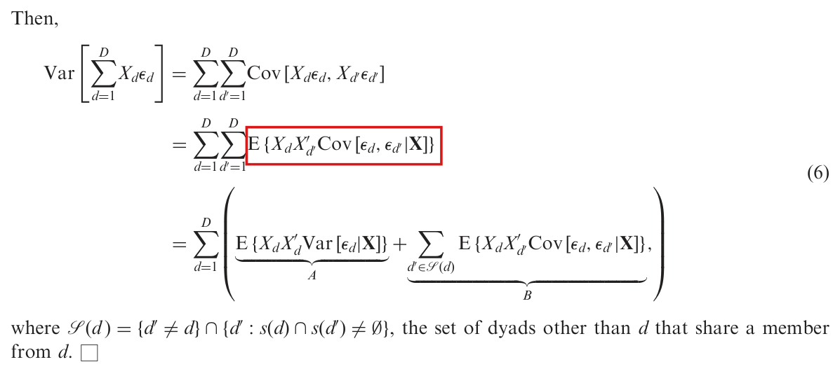
p. 573, equation (6), first two lines:

Var⁡[∑d=1DXdϵd]=∑d=1D∑d′=1DCov⁡[Xdϵd,Xd′ϵd′]=∑d=1D∑d′=1DE{XdXd′′Cov⁡[ϵd,ϵd′∣X]}\operatorname{Var}\Big[\sum_{d=1}^{D}X_d\epsilon_d\Big]=\sum_{d=1}^{D}\sum_{d'=1}^{D}\operatorname{Cov}[X_d\epsilon_d,X_{d'}\epsilon_{d'}]=\sum_{d=1}^{D}\sum_{d'=1}^{D}\mathrm{E}\{X_dX_{d'}'\colorbox{#ffe58a}{$\displaystyle \operatorname{Cov}[\epsilon_d,\epsilon_{d'}|\mathbf{X}]$}\}
The problem

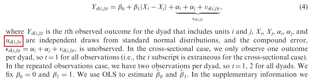
The left side of (2) is the variance of the score sum ∑dXdϵd\sum_dX_d\epsilon_d over the random sample of units. The right side is built from variances and covariances of the residuals that are conditional on the whole design matrix X\mathbf{X}. The two sides agree when E[ϵd∣X]=0\mathrm{E}[\epsilon_d\mid\mathbf{X}]=0, which the paper does not assume. It defines β\beta as the coefficient of the population least-squares fit, “allowing for possible non-linearity in the true relationship between E[Yd(i,j)∣Xd(i,j)]\mathrm{E}[Y_{d(i,j)}|X_{d(i,j)}] and Xd(i,j)X_{d(i,j)}” (p. 566), and footnote 2 (p. 565) says that “the derivation is robust to violations of the assumption that the regression specification is correct for the conditional expectation”. This definition implies that E[Xdϵd]=0\mathrm{E}[X_d\epsilon_d]=0, but does not imply that the conditional mean of ϵd\epsilon_d is zero. In that setting the step from the first to the second line of (6) drops the matrix MN=Var⁡(E[∑dXdϵd∣X])M_N=\operatorname{Var}(\mathrm{E}[\sum_dX_d\epsilon_d\mid\mathbf{X}]), the variance of the conditional mean of the score sum. This matrix is positive semidefinite and need not vanish. In the example below it is of order N3N^3, the order of the variance itself. There the right side of (2) is zero, and the limiting variance is positive definite. The third line of (6) and equation (2) also discard the conditional covariances of dyads that share no unit. The independence of such dyads does not by itself justify this step, which plays no role in the example.

The matrix Σ\Sigma in Appendix B (p. 573) and the limits VrV_r of Corollary 1 (p. 568) and VwV_w of Corollary 2 (p. 576) are defined in the same conditional form, and they are wrong for the same reason. The estimator (3) is built from products of fitted residuals and does not use (2). In (2) the letter E of term BB is printed in the summation subscript; this misprint is the subject of P018-N001.

Evidence an exact counterexample

The evidence is a derivation and an exact counterexample. I write hd=Xdϵdh_d=X_d\epsilon_d for the score of dyad dd and md=E[ϵd∣X]m_d=\mathrm{E}[\epsilon_d\mid\mathbf{X}]. By the definition of β\beta, I have E[hd]=0\mathrm{E}[h_d]=0. Then

Var⁡[∑d=1Dhd]=∑d=1D∑d′=1DE[hdhd′′].\operatorname{Var}\Big[\sum_{d=1}^{D}h_d\Big]=\sum_{d=1}^{D}\sum_{d'=1}^{D}\mathrm{E}[h_dh_{d'}'].

If dd and d′d' share no unit, then hdh_d and hd′h_{d'} are functions of disjoint sets of sampled units. They are independent, and E[hdhd′′]=E[hd]E[hd′]′=0\mathrm{E}[h_dh_{d'}']=\mathrm{E}[h_d]\mathrm{E}[h_{d'}]'=0. The remaining pairs are d′=dd'=d and d′∈S(d)d'\in\mathcal{S}(d), and I obtain equation (2) as corrected below. To compare with the printed form, note that XdX_d is a function of X\mathbf{X}, so that E[hd∣X]=Xdmd\mathrm{E}[h_d\mid\mathbf{X}]=X_dm_d. By the law of total covariance, I have

Cov⁡[hd,hd′]=E{XdXd′′Cov⁡[ϵd,ϵd′∣X]}+E{XdXd′′mdmd′}.\operatorname{Cov}[h_d,h_{d'}]=\mathrm{E}\{X_dX_{d'}'\operatorname{Cov}[\epsilon_d,\epsilon_{d'}\mid\mathbf{X}]\}+\mathrm{E}\{X_dX_{d'}'m_dm_{d'}\}.

Summing over all pairs (d,d′)(d,d'), I obtain

Var⁡[∑d=1Dhd]=∑d=1D∑d′=1DE{XdXd′′Cov⁡[ϵd,ϵd′∣X]}+MN,MN=Var⁡(∑d=1DXdmd).\operatorname{Var}\Big[\sum_{d=1}^{D}h_d\Big]=\sum_{d=1}^{D}\sum_{d'=1}^{D}\mathrm{E}\{X_dX_{d'}'\operatorname{Cov}[\epsilon_d,\epsilon_{d'}\mid\mathbf{X}]\}+M_N,\qquad M_N=\operatorname{Var}\Big(\sum_{d=1}^{D}X_dm_d\Big).

The first term on the right is the second line of (6). The matrix MNM_N is positive semidefinite, and it vanishes when md=0m_d=0 for every dd.

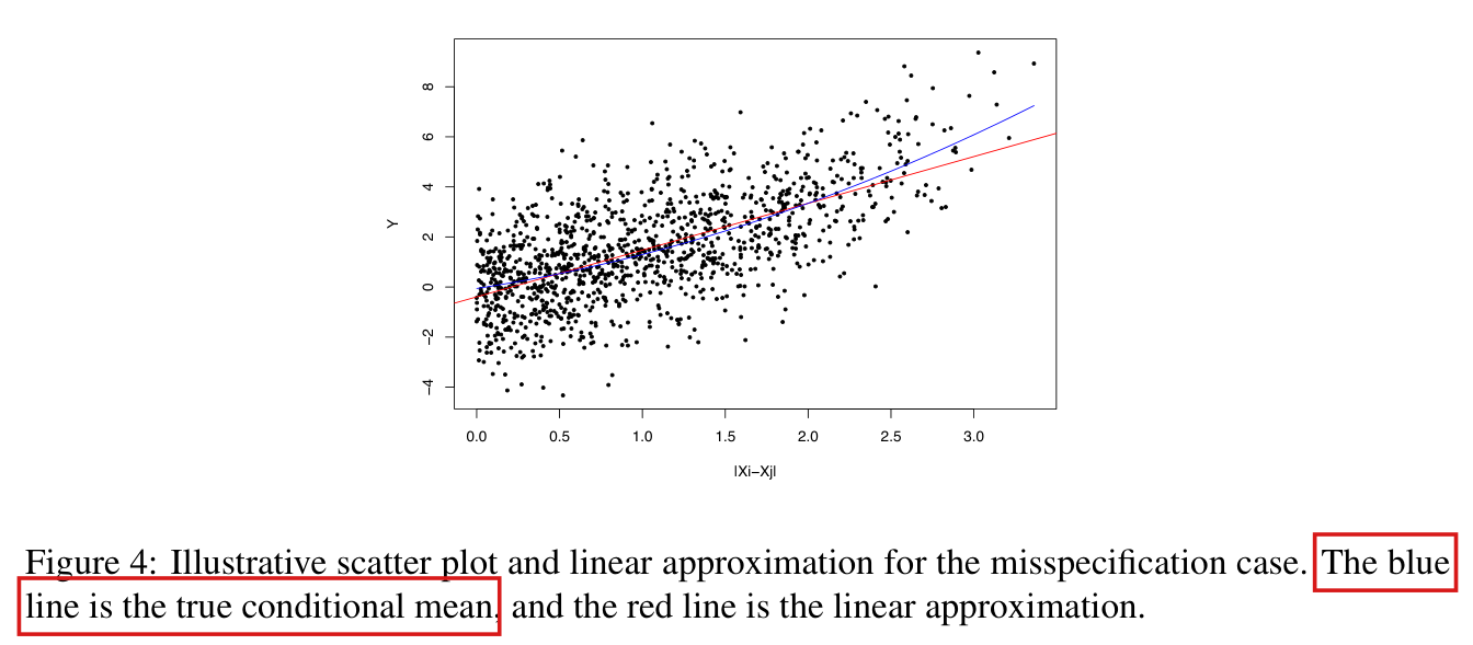
For the counterexample, fix N≥3N\ge3, let Z1,…,ZNZ_1,\dots,Z_N be independent and uniform on [−1,1][-1,1], and for i<ji<j set Xij=(1, 2+Zi+Zj)′X_{ij}=(1,\,2+Z_i+Z_j)' and Yij=(Zi+Zj)2Y_{ij}=(Z_i+Z_j)^2. The data are bounded, the design matrix has rank two with probability one, and

Q=E[XijXij′]=(12214/3),β=(2/30),ϵij=(Zi+Zj)2−23.Q=\mathrm{E}[X_{ij}X_{ij}']=\begin{pmatrix}1&2\\2&14/3\end{pmatrix},\qquad\beta=\begin{pmatrix}2/3\\0\end{pmatrix},\qquad\epsilon_{ij}=(Z_i+Z_j)^2-\frac{2}{3}.

Since ϵij\epsilon_{ij} is a function of XijX_{ij}, every conditional variance and covariance in (2) is zero, and the right side of (2) is the zero matrix for every NN. Exact integration gives

H=E[h12h12′]=(28/4556/4556/453448/945),Γ=E[h12h13′]=(4/458/458/45632/945).H=\mathrm{E}[h_{12}h_{12}']=\begin{pmatrix}28/45&56/45\\56/45&3448/945\end{pmatrix},\qquad\Gamma=\mathrm{E}[h_{12}h_{13}']=\begin{pmatrix}4/45&8/45\\8/45&632/945\end{pmatrix}.

There are DD pairs with d′=dd'=d and N(N−1)(N−2)N(N-1)(N-2) ordered pairs of distinct dyads that share a unit, and I have

Var⁡[∑d=1Dhd]=DH+N(N−1)(N−2)Γ.\operatorname{Var}\Big[\sum_{d=1}^{D}h_d\Big]=DH+N(N-1)(N-2)\Gamma.

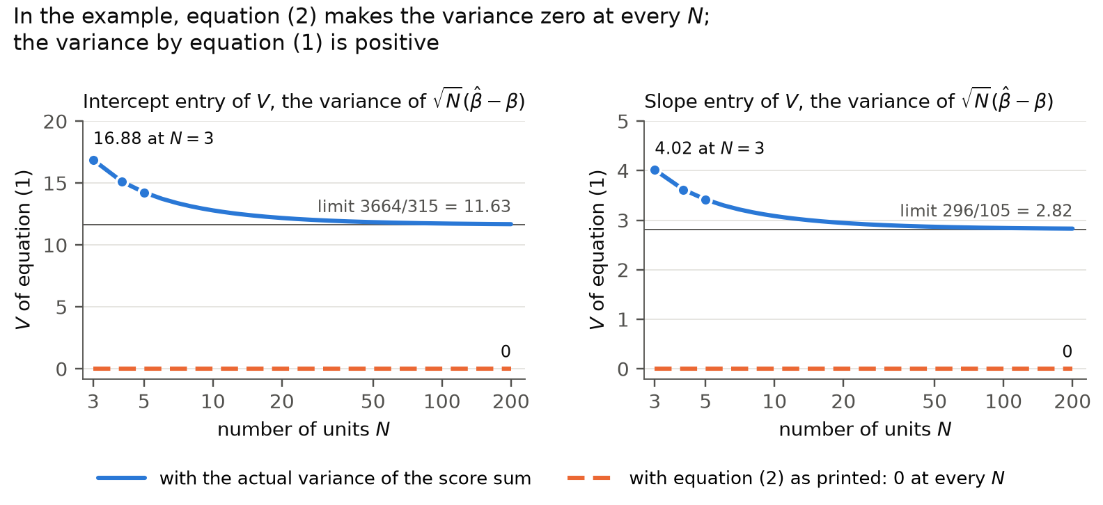
The table lists this matrix for N=3,4,5N=3,4,5, where it was also computed by integrating the square of the score sum directly. As N→∞N\to\infty, the matrix (N/D2)Var⁡[∑dhd](N/D^2)\operatorname{Var}[\sum_dh_d] converges to 4Γ4\Gamma. Then equation (1) implies that

V→4Q−1ΓQ−1=(3664/315−592/105−592/105296/105).V\to4Q^{-1}\Gamma Q^{-1}=\begin{pmatrix}3664/315&-592/105\\-592/105&296/105\end{pmatrix}.

The limit has determinant 4736/47254736/4725 and is positive definite, while the right side of (2) as printed is the zero matrix. A derivation shows that, in this example, NV^N\hat V converges in probability to the same limit, where V^\hat V is the estimator (3). A second example was checked separately, with ZiZ_i uniform on [0,1][0,1], Xij=(1, Zi+Zj)′X_{ij}=(1,\,Z_i+Z_j)' and the same YijY_{ij}. There β=(−5/6,2)′\beta=(-5/6,2)', the right side of (2) is again zero, and the limit of VV is the positive definite matrix with rows (229/315, −74/105)(229/315,\,-74/105) and (−74/105, 74/105)(-74/105,\,74/105).

The variance of the score sum ∑dXdϵd\sum_dX_d\epsilon_d in the first example: exact entries, and the value that equation (2) gives as printed.
NNentry (1,1)(1,1)entry (1,2)(1,2)entry (2,2)(2,2)every entry by (2) as printed
312/512/524/524/54712/3154712/3150
488/1588/15176/15176/151328/351328/350
5104/9104/9208/9208/914480/18914480/1890

The examples show that the omitted term can be of the order of the variance itself. They do not show that it is nonzero for every nonlinear conditional mean.

What survives

Equation (1), the definition of β\beta and the OLS estimator are unaffected, and so is Proposition 2, which is an algebraic identity. The estimator (3) and its repeated and weighted versions are products of fitted residuals and do not use (2). No reported number from the simulations or the applications is shown to be wrong. The correction adds no assumption and changes neither the estimand nor the estimator. What changes is the formula (2), the second and third lines of (6), the definition of Σ\Sigma in Appendix B and the limits VrV_r and VwV_w. The proof in Appendix B is the subject of P018-E006, and the displays of VrV_r and VwV_w have further misprints, treated in P018-E004.

Corrected

“Lemma 1. Suppose data and β^\hat\beta as defined above: the units i=1,…,Ni=1,\dots,N are a random (i.i.d.) sample; the data are the D=N(N−1)/2D=N(N-1)/2 dyads d(i,j)d(i,j); YdY_d and the kk-vector XdX_d, which includes the constant, are determined by the characteristics of the two units of dd and have support bounded in a finite interval; the usual rank conditions on X\mathbf{X} hold; β\beta is the coefficient of the population least-squares fit, with residual ϵd=Yd−Xd′β\epsilon_d=Y_d-X_d'\beta, so that E[Xdϵd]=0\mathrm{E}[X_d\epsilon_d]=0 while E[ϵd∣X]\mathrm{E}[\epsilon_d\mid\mathbf{X}] need not be zero; and β^=(X′X)−1X′Y\hat\beta=(\mathbf{X}'\mathbf{X})^{-1}\mathbf{X}'Y. As N→∞N\to\infty, the asymptotic distribution of N(β^−β)\sqrt{N}(\hat\beta-\beta) has mean zero and variance

V=ND2 E[XdXd′]−1Var⁡[∑d=1DXdϵd]E[XdXd′]−1,(1)V=\frac{N}{D^2}\,\mathrm{E}[X_dX_d']^{-1}\operatorname{Var}\Big[\sum_{d=1}^{D}X_d\epsilon_d\Big]\mathrm{E}[X_dX_d']^{-1},\qquad(1)

with

Var⁡[∑d=1DXdϵd]=∑d=1D(E{XdXd′ϵd2}⏟A+∑d′∈S(d)E{XdXd′′ϵdϵd′}⏟B),(2)\operatorname{Var}\Big[\sum_{d=1}^{D}X_d\epsilon_d\Big]=\sum_{d=1}^{D}\Big(\underbrace{\mathrm{E}\{X_dX_d'\colorbox{#ffe58a}{$\displaystyle \epsilon_d^2$}\}}_{A}+\underbrace{\sum_{d'\in\mathcal{S}(d)}\mathrm{E}\{X_dX_{d'}'\colorbox{#ffe58a}{$\displaystyle \epsilon_d\epsilon_{d'}$}\}}_{B}\Big),\qquad(2)

where S(d)={d′≠d}∩{d′:s(d)∩s(d′)≠∅}\mathcal{S}(d)=\{d'\ne d\}\cap\{d':s(d)\cap s(d')\ne\emptyset\}, the set of dyads other than dd that share a member from dd.”

In equation (6), the second line becomes ∑d∑d′E{XdXd′′ϵdϵd′}\sum_{d}\sum_{d'}\mathrm{E}\{X_dX_{d'}'\colorbox{#ffe58a}{$\epsilon_d\epsilon_{d'}$}\} and the third line becomes the right side of (2) as corrected. Equivalently, the second line of (6) may be kept as printed if Var⁡(E[∑dXdϵd∣X])\operatorname{Var}(\mathrm{E}[\sum_dX_d\epsilon_d\mid\mathbf{X}]) is added to it. In Σ\Sigma of Appendix B, in VrV_r and in VwV_w, the conditional variances and covariances are replaced in the same way by the second moments of the scores, which are Xd′ϵdX_d'\epsilon_d for repeated observations (with XdX_d a T(d)×kT(d)\times k regressor matrix and ϵd\epsilon_d a T(d)T(d)-vector of residuals) and wdXdϵdw_dX_d\epsilon_d for weighted observations.

Crop of Lemma 1 with equations (1) and (2). Equation (2) sets the variance of the sum of X_d epsilon_d equal to a sum over d of two terms labelled A and B. Red boxes mark 'Var[epsilon_d | X]' inside term A and 'Cov[epsilon_d, epsilon_d-prime | X]' inside term B. The letter E of term B is printed in the summation subscript.
Lemma 1, p. 566 (PDF p. 3). The marks are on the conditional variance in term AA and on the conditional covariance in term BB of equation (2).
Crop of equation (6), a chain of three equalities for the variance of the sum of X_d epsilon_d. The first line is a double sum of Cov[X_d epsilon_d, X_d-prime epsilon_d-prime]. A red box marks the summand of the second line, the expectation of X_d X_d-prime-transpose times Cov[epsilon_d, epsilon_d-prime | X]. The third line repeats the right side of equation (2), with E in front of the braces in both terms.
Appendix A, equation (6), p. 573 (PDF p. 10). The mark is on the second line, where the covariances of the scores are replaced by expectations of conditional covariances of the residuals.
Two line charts side by side, one for the intercept entry and one for the slope entry of V. The horizontal axis is the number of units N, from 3 to 200 on a logarithmic scale. In the left chart a blue curve falls from 16.88 at N = 3 to 11.68 at N = 200, toward a grey horizontal line at 11.63. In the right chart a blue curve falls from 4.02 at N = 3 to 2.83 at N = 200, toward a grey horizontal line at 2.82. In both charts an orange dashed line lies at zero for every N, the value given by equation (2) as printed.
The intercept and slope entries of VV in equation (1) in the first example, for NN from 3 to 200 units. The blue curves use the exact variance of the score sum, with dots at N=3,4,5N=3,4,5, where it was also obtained by direct integration, and the grey lines are the limits 3664/3153664/315 and 296/105296/105. The orange dashed lines are the value that results when equation (2) is used as printed, zero at every NN.

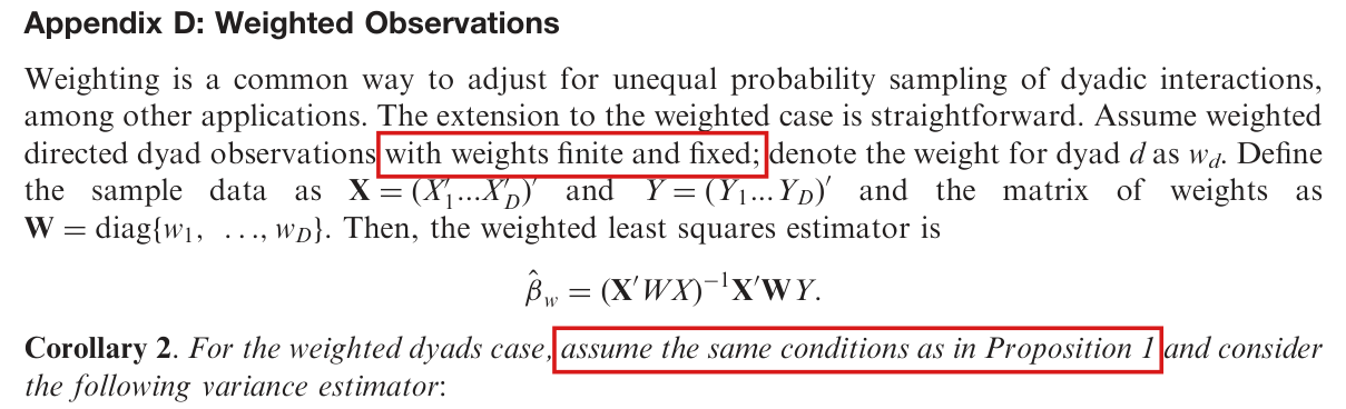
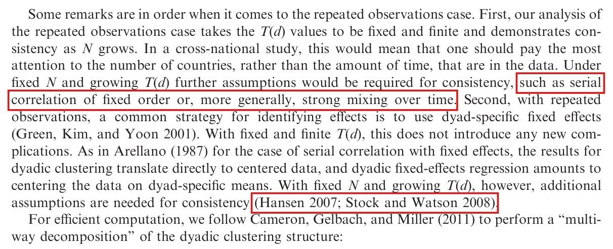
Corollary 2 needs the weights to be bounded after a common rescaling and the rescaled weighted design to have a positive definite limit; weights that are only finite and fixed do not suffice. Corollary 1 also needs uniformly bounded T(d)T(d), a positive definite limiting design matrix and a condition on products of dyad-score means when record kinds follow different laws.

Appendix D and Corollary 2, p. 575 (PDF p. 12); also the repeated-observations setting before Corollary 1, p. 567 (PDF p. 4)

Classification before my review (the classification when the audit was first completed, before I reviewed it): Error, Minor (entry P018-E003).

See also under Formal statements (Lean): P018-T9, P018-T10, P018-T28

My comment on this entry

Revised: see the history of this entry.

As printed

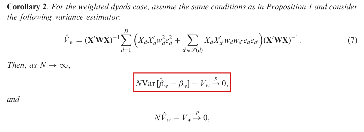
P. 575: Assume weighted directed dyad observations with weights finite and fixed; denote the weight for dyad dd as wdw_d. […] Corollary 2. For the weighted dyads case, assume the same conditions as in Proposition 1 and consider the following variance estimator:

V^w=(X′WX)−1∑d=1D(XdXd′wd2ed2+∑d′∈S(d)XdXd′′wdwd′eded′)(X′WX)−1.(7)\hat V_w=(\mathbf X'\mathbf W\mathbf X)^{-1}\sum_{d=1}^{D}\Big(X_dX_d'w_d^2e_d^2+\sum_{d'\in\mathcal S(d)}X_dX_{d'}'w_dw_{d'}e_de_{d'}\Big)(\mathbf X'\mathbf W\mathbf X)^{-1}.\qquad(7)

Then, as N→∞N\to\infty, NVar⁡[β^w−βw]−Vw→p0N\operatorname{Var}[\hat\beta_w-\beta_w]-V_w\overset{p}{\to}0, and NV^w−Vw→p0N\hat V_w-V_w\overset{p}{\to}0,

P. 567: Formally, suppose that for each dyad dd observations are indexed by t=1,…,T(d)t=1,\dots,T(d), where the T(d)T(d) values are fixed and finite.

The problem

The conditions of Proposition 1 concern the unweighted design: bounded support and the rank of X\mathbf X. They do not control the weighted design X′WX\mathbf X'\mathbf W\mathbf X. Weights that are positive, fixed and uniformly bounded can place almost all of the weight on a few units. Then β^w\hat\beta_w does not converge, and the two limits stated in Corollary 2 cannot both hold for any target.

For repeated observations, “fixed and finite” read dyad by dyad allows the T(d)T(d) to grow across dyads, with the same effect. The discussion on p. 568 indicates that a bound uniform over dyads is meant, and the correction states it. Even with a uniform repetition bound, different record kinds, such as years or directions, may follow different laws. The stacked population normal equations center the total score, but need not give each dyad a mean-zero block score. The estimator sums score products over overlapping dyads, so these products can include a nonvanishing contribution from the dyad-score means that is absent from the covariance target. The correction specifies one common data function per record kind, convergence of the normalized expected design matrix to a positive definite limit, and convergence to zero of the normalized sum of these mean products.

Evidence an exact counterexample

The evidence is an exact counterexample to Corollary 2 as printed. Let A1,A2,…A_1,A_2,\dots be independent with P(Ai=1)=P(Ai=−1)=1/2P(A_i=1)=P(A_i=-1)=1/2, and for i<j≤Ni<j\le N let Xij=1X_{ij}=1, Yij=Ai+AjY_{ij}=A_i+A_j and wij=2−i−jw_{ij}=2^{-i-j}. The weights are positive, fixed and at most 1/81/8. All data are bounded, X′X/D=1\mathbf X'\mathbf X/D=1 and βw=0\beta_w=0, while X′WX/D→0\mathbf X'\mathbf W\mathbf X/D\to0. The estimator is β^w=∑ici,NAi\hat\beta_w=\sum_ic_{i,N}A_i with c1,N=3/{4(1−2−N)}≥3/4c_{1,N}=3/\{4(1-2^{-N})\}\ge3/4. Since the signs are independent with variance one, I have

Var⁡(β^w)=∑i=1Nci,N2≥916for all N≥2,Var⁡(β^w)→3635.\operatorname{Var}(\hat\beta_w)=\sum_{i=1}^{N}c_{i,N}^2\ge\frac9{16}\quad\text{for all }N\ge2,\qquad\operatorname{Var}(\hat\beta_w)\to\frac{36}{35}.

At N=8N=8 the variance equals 56098/5397556098/53975, which is about 1.0391.039. On the event A1=⋯=A8=1A_1=\dots=A_8=1, which has probability 1/2561/256, I have ∣V^w∣≤1/16|\hat V_w|\le1/16 for every N≥8N\ge8. Combining the two bounds, I obtain

P(∣NV^w−NVar⁡(β^w)∣≥N2)≥1256for every N≥8.P\Big(\big|N\hat V_w-N\operatorname{Var}(\hat\beta_w)\big|\ge\frac N2\Big)\ge\frac1{256}\quad\text{for every }N\ge8.

The two limits of Corollary 2 would imply that this probability tends to zero. With T(i,j)=2i+jT(i,j)=2^{i+j} identical observations per dyad and no weights, the estimator and the sandwich of Corollary 1 have the same joint distribution as in the weighted example, after the order of the units is reversed. A uniform bound on the T(d)T(d) excludes this second example.

What survives

The estimator (7), the estimand and the algebraic identity of Proposition 2 are unchanged, and the example does not concern the cross-sectional result without weights: the unweighted estimator in the example has variance 4/N4/N. The simulations use T=2T=2 for every dyad and the application has at most 90 years per dyad, which is compatible with bounded T(d)T(d). The added conditions restrict the weights that the corollary covers, and conditions of the same form are needed for the extension to generalized linear models. The conditions are sufficient ones; I do not claim that they are the weakest.

Corrected

P. 575: Assume weighted directed dyad observations with weights fixed and such that, for some constants aN>0a_N>0 and C<∞C<\infty, 0<wd/aN≤C0<w_d/a_N\le C for all dyads dd and all NN; denote the weight for dyad dd as wdw_d. […] Corollary 2. For the weighted dyads case, assume the same conditions as in Proposition 1, and assume that the matrices D−1∑d=1DE[(wd/aN)XdXd′]D^{-1}\sum_{d=1}^{D}\mathrm E[(w_d/a_N)X_dX_d'] converge to a positive definite limit, and consider the variance estimator (7). Then, as N→∞N\to\infty, the conclusions are those printed, with the target VwV_w as corrected in P018-E004 and the first conclusion requiring uniform integrability of N∥β^w−βw∥2N\|\hat\beta_w-\beta_w\|^2 (P018-N004).

P. 567: Formally, suppose that for each dyad dd observations are indexed by t=1,…,T(d)t=1,\dots,T(d), where the T(d)T(d) values are fixed and bounded uniformly in dd and NN.

For the repeated-data consistency conclusion, for each record kind tt, one common measurable function of the two unit characteristics determines (Xdt,Ydt)(X_{dt},Y_{dt}), independently of NN and dd wherever that record exists. Write LN=∑dTN(d)L_N=\sum_dT_N(d), qd,N=Xd′ϵdq_{d,N}=X_d'\epsilon_d, md,N=E[qd,N]m_{d,N}=\mathrm E[q_{d,N}] and Hr,N=LN−1∑dE[Xd′Xd]H_{r,N}=L_N^{-1}\sum_d\mathrm E[X_d'X_d], where ϵd\epsilon_d is the vector of population residuals from the stacked projection. In addition to the uniform repetition bound, assume that Hr,N→HrH_{r,N}\to H_r with HrH_r positive definite and that

NLN2∑(d,f): s(d)∩s(f)≠∅md,Nmf,N′→0.\colorbox{#ffe58a}{$\displaystyle \frac{N}{L_N^2}\sum_{(d,f):\,s(d)\cap s(f)\ne\emptyset}m_{d,N}m_{f,N}'\to0.$}

The overlap sum is ordered and includes d=fd=f. Then NV^r−Vr→0N\hat V_r-V_r\to0 in probability for the corrected target

Vr=NLN2Hr,N−1Var⁡[∑dqd,N]Hr,N−1.V_r=\frac{N}{L_N^2}H_{r,N}^{-1}\operatorname{Var}\Bigl[\sum_dq_{d,N}\Bigr]H_{r,N}^{-1}.

The stacked population normal equations give ∑dmd,N=0\sum_dm_{d,N}=0 for all sufficiently large NN; they do not imply this overlap mean-product condition.

Under the weight conditions above each rescaled score (wd/aN)Xdϵd(w_d/a_N)X_d\epsilon_d is bounded, and the counts of dependent pairs in the corrected proof of Proposition 1 (P018-E006) give the same rates for the weighted sums. For the weights wij=2−i−jw_{ij}=2^{-i-j} of the example, the first condition forces aN≥1/(8C)a_N\ge1/(8C). Then D−1∑dwd/aN≤8C X′WX/D→0D^{-1}\sum_dw_d/a_N\le8C\,\mathbf X'\mathbf W\mathbf X/D\to0, and the second condition fails.

Crop of the heading Appendix D: Weighted Observations, the paragraph that follows, the display of the weighted least squares estimator, and the first two lines of Corollary 2. Red boxes mark the words with weights finite and fixed; and the words assume the same conditions as in Proposition 1.
Appendix D, p. 575 (PDF p. 12). The marked phrases are the only conditions on the weights: they are finite and fixed, and the conditions of Proposition 1 are assumed.
Crop of four lines from the paragraph before Corollary 1. A red box marks the words fixed and finite in the clause where the T of d values are fixed and finite.
P. 567 (PDF p. 4), setting for repeated observations. The marked words bound each T(d)T(d) separately and state no bound that is uniform over dyads.
My comment and the history of this entry

Updated after the LLMs rendered a decision. I think this is mostly a regularity condition in context, but I'm fine classifying it as moderate.

  1. Classification before my review (the classification when the audit was first completed, before I reviewed it): Minor error.
  2. Changed by a later check, before my comment was evaluated: Moderate error.
  3. Revised. The repeated-data correction was expanded while the classification was still Minor. When record kinds follow different laws, the stacked normal equations center the total score but need not center each dyad’s score. The correction therefore adds a condition requiring the normalized sum of products of score means over overlapping dyads to tend to zero. The estimator and the score-covariance target are unchanged. P. M. Aronow delegated this decision to the model session that runs the audit, which adopted the amendment recommended by the two checks; this note was written by that session.
  4. Revised. Later, the model session running the audit raised the classification from Minor to Moderate, after P. M. Aronow suggested Moderate and left the final decision to that session. The additional condition on score means is substantive when different record kinds follow different laws, a reading supported by p. 567; it holds automatically when every record follows one common law. The correction, estimator, cross-sectional result and weighted corollary are unchanged. This note was written by that session.
  5. I commented.
  6. Independent evaluation. My comment accepts the current Moderate classification; no change.

Three steps of the proof of Proposition 1 in Appendix B fail, and the conclusion NV^−V→p0N\hat V-V\overset{p}{\to}0 follows instead from an argument in probability that uses the population scores, a bound for the substitution of fitted residuals, and convergence of the inverse Gram matrix.

Appendix B, proof of Proposition 1, pp. 573–574 (PDF pp. 10–11)

See also under Formal statements (Lean): P018-T3, P018-T4, P018-T27

As printed

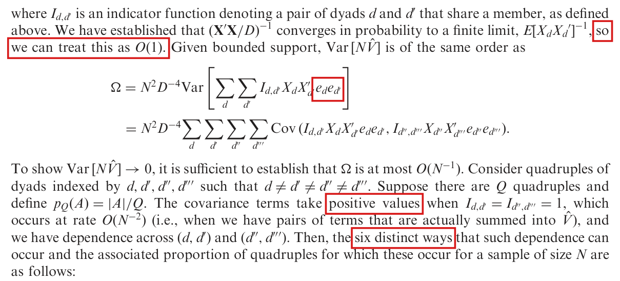
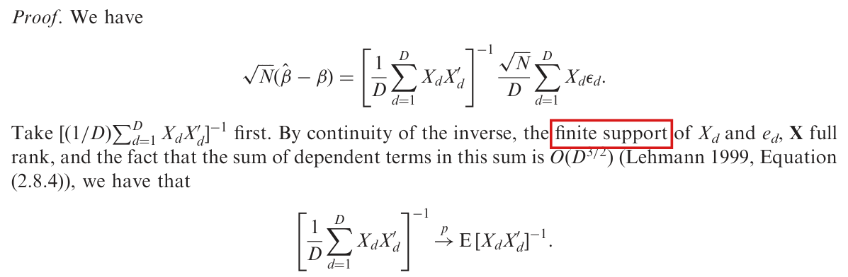
P. 573: Proof. By Chebyshev’s inequality, two conditions are sufficient for NV^−V→p0N\hat V-V\overset{p}{\to}0 as N→∞N\to\infty: (i) E[V^−V]→0\colorbox{#ffe58a}{$\mathrm E[\hat V-V]\to0$} and (ii) Var⁡[NV^−V]=Var⁡[NV^]→0\operatorname{Var}[N\hat V-V]=\operatorname{Var}[N\hat V]\to0 (Lehmann 1999, Theorem 2.1.1). […] We have

E[Σ^]=∑d=1D(E{XdXd′E[ed2∣X]}+∑d′∈S(d)E{XdXd′′E[eded′∣X]})→Σ\mathrm E[\hat\Sigma]=\sum_{d=1}^{D}\Big(\mathrm E\{X_dX_d'\mathrm E[e_d^2\mid\mathbf X]\}+\sum_{d'\in\mathcal S(d)}\mathrm E\{X_dX_{d'}'\mathrm E[e_de_{d'}\mid\mathbf X]\}\Big)\colorbox{#ffe58a}{$\displaystyle \to\Sigma$}

P. 574: by consistency of β^\hat\beta, an implication of Lemma 1. Lemma 1 also established that (X′X/D)−1→pE[XdXd′]−1(\mathbf X'\mathbf X/D)^{-1}\overset{p}{\to}\mathrm E[X_dX_d']^{-1}, while boundedness of XdX_d implies uniform boundedness of E[XdXd′]−1\mathrm E[X_dX_d']^{-1}. Taking these elements together, uniform continuity implies E[V^−V]→0\colorbox{#ffe58a}{$\mathrm E[\hat V-V]\to0$} (cf. White 1980a, Theorem 1). […] We have established that (X′X/D)−1(\mathbf X'\mathbf X/D)^{-1} converges in probability to a finite limit, E[XdXd′]−1E[X_dX_d']^{-1}, so we can treat this as O(1)O(1). Given bounded support, Var⁡[NV^]\operatorname{Var}[N\hat V] is of the same order as

Ω=N2D−4Var⁡[∑d∑d′Id,d′XdXd′′eded′]\Omega=N^2D^{-4}\operatorname{Var}\Big[\sum_d\sum_{d'}I_{d,d'}X_dX_{d'}'\colorbox{#ffe58a}{$\displaystyle e_de_{d'}$}\Big]

[…] The covariance terms take positive values when Id,d′=Id′′,d′′′=1I_{d,d'}=I_{d'',d'''}=1, which occurs at rate O(N−2)O(N^{-2}) (i.e., when we have pairs of terms that are actually summed into V^\hat V), and we have dependence across (d,d′)(d,d') and (d′′,d′′′)(d'',d'''). Then, the six distinct ways that such dependence can occur and the associated proportion of quadruples for which these occur for a sample of size NN are as follows: […]

The problem

Proposition 1 states that NV^−V→0N\hat V-V\to0 in probability, where V^\hat V is the estimator (3). The printed proof attempts to bound the mean and the variance of NV^N\hat V and applies Chebyshev’s inequality. Three of its steps fail.

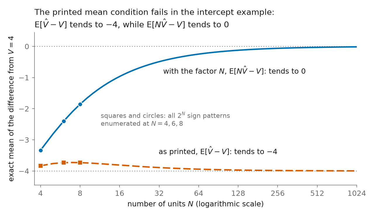
The first is the scaling. With condition (ii), Chebyshev’s inequality requires E[NV^−V]→0\mathrm E[N\hat V-V]\to0. Condition (i) is printed without the factor NN, and p. 574 repeats it in that form. The printed pair of conditions is not sufficient, and in the example below the printed mean tends to −4-4 and not to 00. The display E[Σ^]→Σ\mathrm E[\hat\Sigma]\to\Sigma compares two unnormalized sums, and consistency of β^\hat\beta does not make their difference vanish.

The second concerns the residuals. The ede_d in Σ^\hat\Sigma and Ω\Omega are the fitted residuals ed=Yd−Xd′β^e_d=Y_d-X_d'\hat\beta, which p. 566 distinguishes from the population residuals ϵd\epsilon_d. Since β^\hat\beta depends on every unit, the products eded′e_de_{d'} and ed′′ed′′′e_{d''}e_{d'''} can be correlated even when the two pairs of dyads have no unit in common. Each of the six cases on p. 574 requires a common unit, and the six cases therefore do not exhaust the covariances that are not zero. These covariances can also be negative, and the count has to bound absolute values.

The third concerns the inverse Gram matrix. The proof treats the random matrix (X′X/D)−1(\mathbf X'\mathbf X/D)^{-1} as a constant of order one inside the mean and the variance of NV^N\hat V. Convergence in probability implies that this matrix is bounded in probability, but not that its moments are bounded. Boundedness of XdX_d bounds E[XdXd′]\mathrm E[X_dX_d'] and not its inverse. The inverse is finite because of the rank condition of p. 566.

Evidence an exact counterexample

The evidence is an exact counterexample to the printed steps and a derivation of the proposition by another route, given in the corrected proof below. Let U1,…,UNU_1,\dots,U_N be independent with P(Ui=1)=P(Ui=−1)=1/2P(U_i=1)=P(U_i=-1)=1/2, and for each of the D=N(N−1)/2D=N(N-1)/2 dyads let Xij=1X_{ij}=1 and Yij=Ui+UjY_{ij}=U_i+U_j. In this example β=0\beta=0 and X′X=D\mathbf X'\mathbf X=D, all variables are bounded, and V=4V=4. The fitted residuals are eij=Ui+Uj−2Uˉe_{ij}=U_i+U_j-2\bar U, where Uˉ\bar U is the mean of the UiU_i. Computing the moments directly, I obtain

Σ=N(N−1)2,E[Σ^]=(N−1)(N−2)(N−3),E[Σ^]−Σ=(−4N+6)(N−1)→−∞,\Sigma=N(N-1)^2,\qquad\mathrm E[\hat\Sigma]=(N-1)(N-2)(N-3),\qquad\mathrm E[\hat\Sigma]-\Sigma=(-4N+6)(N-1)\to-\infty,
E[NV^]=4(N−2)(N−3)N(N−1)→4,E[V^−V]→−4,Var⁡[NV^]=32(N−2)2(N−3)2N3(N−1)3→0.\mathrm E[N\hat V]=\frac{4(N-2)(N-3)}{N(N-1)}\to4,\qquad\mathrm E[\hat V-V]\to-4,\qquad\operatorname{Var}[N\hat V]=\frac{32(N-2)^2(N-3)^2}{N^3(N-1)^3}\to0.

By the first and last limits of the second display and Chebyshev’s inequality, I have NV^→4=VN\hat V\to4=V in probability, as Proposition 1 states. Both printed limits of means are false in this example. For N≥6N\ge6, I find

Cov⁡(e12e13, e45e46)=16(N+6)N3,\operatorname{Cov}(e_{12}e_{13},\,e_{45}e_{46})=\frac{16(N+6)}{N^3},

which equals 7/167/16 at N=8N=8, although the unit sets {1,2,3}\{1,2,3\} and {4,5,6}\{4,5,6\} are disjoint. The same covariance for the population residuals is zero. At N=8N=8, I also have Cov⁡(e12e13, e14e15)=−1/16\operatorname{Cov}(e_{12}e_{13},\,e_{14}e_{15})=-1/16. Enumeration of all 2N2^N sign patterns in exact arithmetic for N=4,6,8N=4,6,8 agrees with these formulas.

Exact values in the example, for which V=4V=4.
QuantityN=4N=4N=6N=6N=8N=8
Σ\Sigma3636150150392392
E[Σ^]\mathrm E[\hat\Sigma]666060210210
E[V^−V]\mathrm E[\hat V-V], as printed in (i)−23/6-23/6−56/15-56/15−209/56-209/56
E[NV^−V]\mathrm E[N\hat V-V]−10/3-10/3−12/5-12/5−13/7-13/7
Var⁡[NV^]\operatorname{Var}[N\hat V]2/272/2764/37564/375225/1372225/1372
Cov⁡(e12e13, e45e46)\operatorname{Cov}(e_{12}e_{13},\,e_{45}e_{46})–8/98/97/167/16

For the third step, let T1,…,TNT_1,\dots,T_N be independent with density t−2t^{-2} on [1,∞)[1,\infty), and let Zi=e−TiZ_i=e^{-T_i} and Xij=(1,Zi+Zj)′X_{ij}=(1,Z_i+Z_j)'. The regressors are bounded, the sample design has full rank almost surely for N≥3N\ge3, and the population Gram matrix is nonsingular. For each k≥1k\ge1, every TiT_i is at least kk with probability k−Nk^{-N}, and then the norm of (X′X/D)−1(\mathbf X'\mathbf X/D)^{-1} is at least e2k/4e^{2k}/4. This implies that the expected norm of this inverse is infinite for every N≥3N\ge3, while the inverse converges in probability to its population value. The example shows that there is no automatic bound on the moments of the inverse. It does not show that NV^N\hat V has infinite moments.

What survives

The estimator (3) and the finite-sample identity of Proposition 2 are unchanged. Proposition 1 holds for VV as defined in equation (1), under the paper’s assumptions and with no new one; the conditional form of Σ\Sigma printed in the proof is corrected in P018-E001. Corollaries 1 and 2 appeal to Proposition 1 and require analogous probability arguments. The same fitted-score issue must be addressed for generalized linear models. These defects establish no change to the reported simulation or application numbers; I have not recalculated them here. The moments of NV^N\hat V and of β^\hat\beta are the subject of P018-N004.

Corrected

Proof of Proposition 1. Assume, as on p. 566, that the units are an i.i.d. sample from a fixed population, that (Xd,Yd)(X_d,Y_d) is a function of the characteristics of the two units of dyad dd, that ∥Xd∥≤CX\|X_d\|\le C_X and YdY_d is bounded, and that Q=E[XdXd′]Q=\mathrm E[X_dX_d'] is nonsingular. Let β\beta be the population least-squares coefficient and ϵd=Yd−Xd′β\epsilon_d=Y_d-X_d'\beta, so that E[Xdϵd]=0\mathrm E[X_d\epsilon_d]=0 and ∣ϵd∣≤Ce|\epsilon_d|\le C_e for a constant CeC_e. Let QN=X′X/DQ_N=\mathbf X'\mathbf X/D and, for residuals r=(rd)r=(r_d), let

MN(r)=ND2∑(d,d′): s(d)∩s(d′)≠∅XdXd′′rdrd′,TN=E[MN(ϵ)]=ND2Var⁡[∑d=1DXdϵd].M_N(r)=\colorbox{#ffe58a}{$\displaystyle \frac{N}{D^2}$}\sum_{(d,d'):\,s(d)\cap s(d')\ne\emptyset}X_dX_{d'}'r_dr_{d'},\qquad T_N=\mathrm E[M_N(\epsilon)]=\frac{N}{D^2}\operatorname{Var}\Big[\sum_{d=1}^{D}X_d\epsilon_d\Big].

The sum runs over ordered pairs of dyads and includes d′=dd'=d. The second expression for TNT_N holds because the scores XdϵdX_d\epsilon_d have mean zero and the scores of two dyads with no common unit are independent. The target of equation (1) is V=Q−1TNQ−1V=Q^{-1}T_NQ^{-1}, and equation (3) reads NV^=QN−1MN(e)QN−1N\hat V=Q_N^{-1}M_N(e)Q_N^{-1}. The proof has four steps, each in probability.

Step 1. Each dyad shares a unit with exactly 2N−32N-3 dyads, itself included. The summands of QNQ_N are bounded and E[QN]=Q\mathrm E[Q_N]=Q, so each entry of QNQ_N has variance at most a constant times D(2N−3)/D2=O(N−1)D(2N-3)/D^2=O(N^{-1}). Chebyshev’s inequality gives QN→QQ_N\to Q in probability, and QN−1→Q−1Q_N^{-1}\to Q^{-1} in probability because QQ is nonsingular. The same count gives D−1∑dXdϵd=Op(N−1/2)D^{-1}\sum_dX_d\epsilon_d=O_p(N^{-1/2}). Hence δN=β^−β=QN−1D−1∑dXdϵd=Op(N−1/2)\delta_N=\hat\beta-\beta=Q_N^{-1}D^{-1}\sum_dX_d\epsilon_d=O_p(N^{-1/2}).

Step 2. The sum in MNM_N has D(2N−3)D(2N-3) terms, so ∥TN∥≤4CX2Ce2\|T_N\|\le4C_X^2C_e^2. Each term involves two or three units, and it is independent of every term that has no unit in common with it. At most 3(N−1)(3N−5)3(N-1)(3N-5) terms have a unit in common with a given term. At most D(2N−3)⋅3(N−1)(3N−5)=O(N5)D(2N-3)\cdot3(N-1)(3N-5)=O(N^5) pairs of terms then have a covariance that is not zero, and each covariance is at most 2CX4Ce42C_X^4C_e^4 in absolute value. For each entry (a,b)(a,b),

Var⁡([MN(ϵ)]ab)≤N2D4 2CX4Ce4 D(2N−3) 3(N−1)(3N−5)=O(N−1),\operatorname{Var}\big([M_N(\colorbox{#ffe58a}{$\displaystyle \epsilon$})]_{ab}\big)\le\frac{N^2}{D^4}\,2C_X^4C_e^4\,D(2N-3)\,3(N-1)(3N-5)=O(N^{-1}),

and Chebyshev’s inequality gives MN(ϵ)−TN→0M_N(\epsilon)-T_N\to0 in probability.

Step 3. Since ed=ϵd−Xd′δNe_d=\epsilon_d-X_d'\delta_N, every pair of dyads satisfies ∣eded′−ϵdϵd′∣≤2CeCX∥δN∥+CX2∥δN∥2|e_de_{d'}-\epsilon_d\epsilon_{d'}|\le2C_eC_X\|\delta_N\|+C_X^2\|\delta_N\|^2. Hence

∥MN(e)−MN(ϵ)∥≤4CX2(2CeCX∥δN∥+CX2∥δN∥2)=op(1).\colorbox{#ffe58a}{$\displaystyle \|M_N(e)-M_N(\epsilon)\|\le4C_X^2\big(2C_eC_X\|\delta_N\|+C_X^2\|\delta_N\|^2\big)$}=o_p(1).

Step 4. By Steps 2 and 3, MN(e)−TN=op(1)M_N(e)-T_N=o_p(1). The identity

NV^−V=QN−1[MN(e)−TN]QN−1+(QN−1−Q−1)TNQN−1+Q−1TN(QN−1−Q−1)N\hat V-V=Q_N^{-1}\big[M_N(e)-T_N\big]Q_N^{-1}+(Q_N^{-1}-Q^{-1})T_NQ_N^{-1}+Q^{-1}T_N(Q_N^{-1}-Q^{-1})

and Step 1 imply that NV^−V→p0N\hat V-V\overset{p}{\to}0, since TNT_N is bounded and QN−1=Op(1)Q_N^{-1}=O_p(1). No mean or variance of QN−1Q_N^{-1} or of NV^N\hat V is used. If QNQ_N is singular on some samples, V^\hat V may be defined arbitrarily there, because the probability of these samples tends to zero.

Crop of the heading Appendix B: Proof of Proposition 1 and the first three lines of the proof. A red box marks condition (i), which reads E of V hat minus V tends to zero.
Appendix B, p. 573 (PDF p. 10), first lines of the proof. The marked condition (i) has no factor NN, while the target and condition (ii) concern NV^N\hat V.
Crop of two displays: the definition of Sigma as a sum over dyads of expected conditional variances and covariances of the population residuals, and the expectation of Sigma hat written with the fitted residuals e. A red box marks the arrow and the symbol Sigma at the end of the second display.
Appendix B, p. 573 (PDF p. 10), last display of the page. The marked limit compares the two sums without normalization.
Crop of the first four lines of page 574. One red box marks the clause boundedness of X d implies uniform boundedness of the inverse of E of X d X d prime. A second red box marks E of V hat minus V tends to zero.
Appendix B, p. 574 (PDF p. 11), first lines. The marked clause infers a bound on the inverse from bounded regressors, and the marked limit again has no factor NN.
Crop of part (ii) of the proof: three lines of text, the two-line display defining Omega as N squared D to the minus four times the variance of a double sum, and a paragraph on quadruples of dyads. Red boxes mark the words so we can treat this as O of one, the product e d e d prime inside the variance, the words positive values, and the words six distinct ways.
Appendix B, p. 574 (PDF p. 11), part (ii) of the proof. Marked: the inverse Gram matrix treated as O(1)O(1) inside a variance, the fitted residuals eded′e_de_{d'} in Ω\Omega, the words “positive values”, and “six distinct ways”.
Line chart with the number of units N from 4 to 1024 on a logarithmic horizontal axis and the exact mean of the difference from V equals 4 on the vertical axis, from minus 4 to 0. A dashed orange curve, labelled as printed, E of V hat minus V, starts at minus 3.83 and settles on the reference line at minus 4. A solid blue curve, labelled with the factor N, E of N V hat minus V, rises from minus 3.33 at N equals 4 to about minus 0.02 at N equals 1024, approaching the reference line at 0. Squares and circles mark the enumerated values at N equals 4, 6 and 8.
The two mean conditions in the example with Xij=1X_{ij}=1 and Yij=Ui+UjY_{ij}=U_i+U_j, for N=4N=4 to 10241024. The mean printed in condition (i) of p. 573 tends to −4-4; with the factor NN it tends to 00. The points at N=4,6,8N=4,6,8 are exact enumerations.

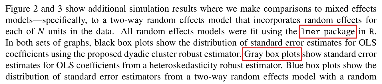
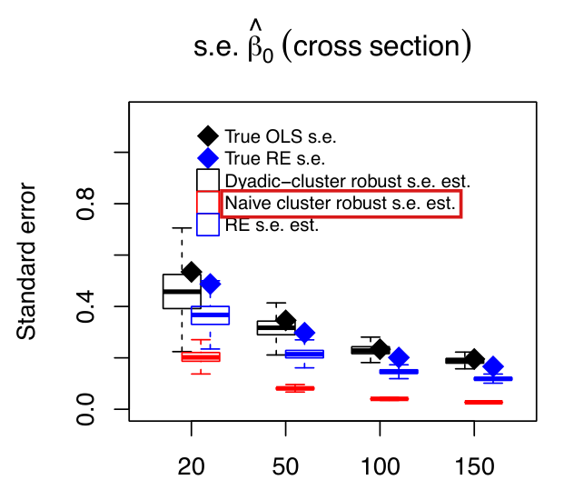
The random effects model fitted in the simulations assigns each unit two independent effects, one for each position in the dyad; it is misspecified even in the normal linear design, and the simulations do not show that its standard errors are consistent or that inference from it is reliable.

Paragraph that begins on p. 569 and continues below Figure 1 on p. 570 (PDF pp. 6–7); Supporting Information, p. 2 (text under Figure 2) and p. 4; Conclusion, p. 572 (PDF p. 9)

See also under Formal statements (Lean): P018-T5, P018-T6, P018-T25

As printed

Main text, pp. 569–570: “Specifically, we compare OLS with dyadic cluster robust standard errors to a two-way random effects model that incorporates normal random effects for each of the NN units (Gelman and Hill 2007). The data-generating process captured above (i.e., expression 4 with normal data) corresponds precisely to the assumptions of a two-way normal random effects model, and so it is no surprise that we find this model to be more efficient than OLS and to produce consistent standard errors.”

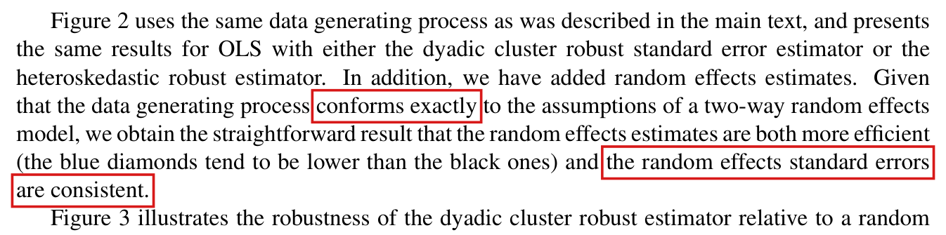
Supporting Information, p. 2: “Given that the data generating process conforms exactly to the assumptions of a two-way random effects model, we obtain the straightforward result that the random effects estimates are both more efficient (the blue diamonds tend to be lower than the black ones) and the random effects standard errors are consistent.”

Conclusion, p. 572: “Our simulations show that a two-way (for cross-sectional data) random effects model can be considerably more efficient and provide reliable inference when the conditional mean is correctly specified.”

The problem

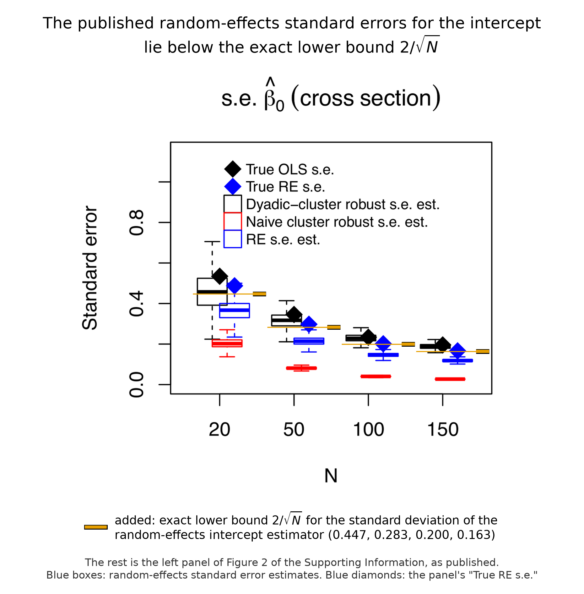
In equation (4) the error of the dyad {i,j}\{i, j\} is αi+αj+νd(i,j)t\alpha_i + \alpha_j + \nu_{d(i,j)t}. Each unit has one effect αi\alpha_i, which enters every dyad that contains the unit. The replication scripts list the lower-numbered unit of each dyad first. They fit the random effects model with the terms (1|dyad1) + (1|dyad2), one for the unit listed first and one for the unit listed second. The two terms are independent random vectors. A unit has one effect when it is listed first and another, independent effect when it is listed second. The dyads {1,2}\{1, 2\} and {2,3}\{2, 3\} share unit 2 in different positions. Their errors have covariance 11 in the simulated data and covariance 00 in the fitted model, for all values of its variance components. The data-generating process does not correspond to the fitted model, whose covariance is wrong at every sample size, even in the normal linear design. The same holds in the design with mild misspecification of the mean (Figure 3 of the Supporting Information). It also holds in the fit with repeated observations, where the added dyad effect does not restore the missing covariance. Two statements of the paper are not supported for the model as fitted. The first is that its standard errors are consistent and its inference reliable when the conditional mean is correct. In Figure 2 of the Supporting Information, the boxes of random effects standard errors for the intercept lie below the plotted standard deviation of the estimates at all four sample sizes. The second is that the failure of these standard errors in Figure 3 comes from the misspecified mean. That comparison changes the mean of a model whose covariance was already misspecified.

Evidence an exact counterexample

The evidence is an exact counterexample with a derivation. For N=3N = 3, I order the dyads as {1,2}\{1,2\}, {1,3}\{1,3\}, {2,3}\{2,3\}. Let τ1\tau_1 and τ2\tau_2 be the variances of the two fitted effects and σ2\sigma^2 the residual variance. The covariance matrix of the simulated errors and that of the fitted model are

(311131113)and(τ1+τ2+σ2τ10τ1τ1+τ2+σ2τ20τ2τ1+τ2+σ2).\begin{pmatrix} 3 & 1 & 1 \\ 1 & 3 & 1 \\ 1 & 1 & 3 \end{pmatrix} \qquad \text{and} \qquad \begin{pmatrix} \tau_1 + \tau_2 + \sigma^2 & \tau_1 & 0 \\ \tau_1 & \tau_1 + \tau_2 + \sigma^2 & \tau_2 \\ 0 & \tau_2 & \tau_1 + \tau_2 + \sigma^2 \end{pmatrix}.

The corner entries differ for every choice of τ1\tau_1, τ2\tau_2 and σ2\sigma^2, and these three dyads occur in every sample. The design matrix that lme4 builds for the two terms also implies this zero covariance.

A wrong covariance alone does not show that the standard error of a coefficient is wrong. In the following example it is. Let the unit covariates be (0,1,3)(0, 1, 3), so that the dyad regressor is (1,3,2)(1, 3, 2), and fix τ1=τ2=σ2=1\tau_1 = \tau_2 = \sigma^2 = 1. The generalised least squares estimator under the fitted covariance reports the intercept variance 71/1671/16. Its variance under the simulated covariance is 379/64379/64. The ratio of the two is 284/379284/379, and the ratio of the standard errors is 0.8660.866. This computation holds the variance components fixed and is not a statement about the fitted model with estimated components.

The variance of the intercept estimator of the fitted model itself has a lower bound. Let αˉ\bar\alpha denote the mean of α1,…,αN\alpha_1, \dots, \alpha_N. Every error contains the term 2αˉ2\bar\alpha, since

αi+αj+νd(i,j)t=2αˉ+(αi−αˉ)+(αj−αˉ)+νd(i,j)t,\alpha_i + \alpha_j + \nu_{d(i,j)t} = 2\bar\alpha + (\alpha_i - \bar\alpha) + (\alpha_j - \bar\alpha) + \nu_{d(i,j)t},

and αˉ\bar\alpha is independent of the other three terms and of the regressors. Adding a constant cc to every outcome leaves the restricted likelihood of the variance components unchanged and adds cc to the estimated intercept. The intercept estimate is therefore the sum of 2αˉ2\bar\alpha and an independent variable, and I have

Var⁡[β^0]≥4Var⁡[αˉ]=4N.\operatorname{Var}[\widehat\beta_0] \ge 4 \operatorname{Var}[\bar\alpha] = \frac{4}{N}.
Exact lower bounds for the variance and the standard deviation of the random effects intercept estimator in the simulation design.
NNVariance, 4/N4/NStandard deviation, 2/N2/\sqrt{N}
20201/51/50.4470.447
50502/252/250.2830.283
1001001/251/250.2000.200
1501502/752/750.1630.163

In the left panel of Figure 2 of the Supporting Information, the boxes of the standard errors of the random effects model lie below these bounds at all four sample sizes. This is a reading of the published figure. The original simulation output is not in the replication files, and no numerical ratio was extracted. The evidence does not establish the limit of the fitted standard errors as NN grows, a particular percentage shortfall, or any effect on the standard errors of the slope.

What survives

The dyadic cluster robust estimator, its theory, the OLS estimates, Figure 1 and the two applications do not use the random effects fit and are not affected. The published figures may still show correctly that the estimates of the random effects model vary less than the OLS estimates. A random effects model with one effect per unit is correctly specified for equation (4); its performance, and the efficiency comparison, would have to be simulated anew. The simulations do not support the statements that the random effects model has consistent standard errors and provides reliable inference. The failure in Figure 3 of the Supporting Information cannot be attributed to the mean alone.

Corrected

Main text, pp. 569–570: “Specifically, we compare OLS with dyadic cluster robust standard errors to a two-way random effects model with independent normal random effects for the first-listed and the second-listed unit of each dyad. The data-generating process captured above (i.e., expression 4 with normal data) has a single effect for each unit, the same in either position, and the fitted model is therefore misspecified in its covariance even with normal data. In these simulations its estimates vary less than the OLS estimates, but its standard errors for the intercept are understated, and the comparison does not demonstrate reliable random effects inference.”

Supporting Information, pp. 2 and 4: the same change, with one addition. The nonlinear design adds misspecification of the conditional mean to a covariance that is already misspecified, and the discrepancy in Figure 3 cannot be attributed to the mean alone.

Conclusion, p. 572: “Our simulations show that a two-way (for cross-sectional data) random effects model can be considerably more efficient. They do not show that it provides reliable inference, because the model fitted was not correctly specified.”

A correctly specified comparison requires a single random effect per unit, entering each dyad through both of its members, and new simulations.

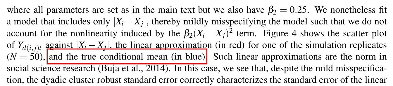
Crop of six lines of text. They read: with normal data) corresponds precisely to the assumptions of a two-way normal random effects model, and so it is no surprise that we find this model to be more efficient than OLS and to produce consistent standard errors. However, as discussed above, such models are sensitive to misspecification. For example, in fitting a linear approximation model to mildly non-linear data, the dyadic cluster robust standard errors continue to be consistent for the coefficients of the linear approximation. The degree of misspecification in this case is not extreme (as illustrated in the. Red outlines surround the words corresponds precisely and the words consistent standard errors.
Text below Figure 1, p. 570 (PDF p. 7), the continuation of the paragraph that begins on p. 569. The outlines mark “corresponds precisely” and “consistent standard errors.”
Crop of eight lines of text. They read: Figure 2 uses the same data generating process as was described in the main text, and presents the same results for OLS with either the dyadic cluster robust standard error estimator or the heteroskedastic robust estimator. In addition, we have added random effects estimates. Given that the data generating process conforms exactly to the assumptions of a two-way random effects model, we obtain the straightforward result that the random effects estimates are both more efficient (the blue diamonds tend to be lower than the black ones) and the random effects standard errors are consistent. Figure 3 illustrates the robustness of the dyadic cluster robust estimator relative to a random. Red outlines surround the words conforms exactly and the words the random effects standard errors are consistent.
Supporting Information, p. 2, paragraph under Figure 2. The outlines mark “conforms exactly” and “the random effects standard errors are consistent.”
Crop of five lines of text. They read: A cost of the robust approach is efficiency. Our simulations show that a two-way (for cross-sectional data) random effects model can be considerably more efficient and provide reliable inference when the conditional mean is correctly specified. Our robust estimator could provide the basis of a test for misspecification (White 1980a, 1981; King and Roberts 2015). If there is little evidence of misspecification, the random effects estimator would be a reasonable choice given its efficiency. A red outline in two parts surrounds the words provide reliable inference when the conditional mean is correctly specified.
Conclusion, p. 572 (PDF p. 9). The outline marks the claim of reliable inference when the conditional mean is correctly specified.
The published plot titled s.e. beta-hat 0 (cross section), with vertical axis Standard error labelled 0.0, 0.4 and 0.8 and horizontal axis N at 20, 50, 100 and 150. At each N it shows a black box and a black diamond, a blue box and a blue diamond, and a red box near the bottom. Added to the plot at each N is a short orange horizontal mark at the height 2 over the square root of N: 0.447, 0.283, 0.200 and 0.163. At each of the four sample sizes the blue box lies below the orange mark, and the blue diamond lies at about the height of the mark or slightly above it. A heading above the plot reads: The published random-effects standard errors for the intercept lie below the exact lower bound 2 over the square root of N. A note below says that the orange marks were added and that the rest is the panel as published.
Figure 2 of the Supporting Information, left panel (p. 2), as published, with the exact lower bound 2/N2/\sqrt{N} for the standard deviation of the random effects intercept estimator added in orange. At each sample size the blue box of random effects standard errors lies below the bound.

Minor (17)

Real but inconsequential, for example a misprint that does not change a result.

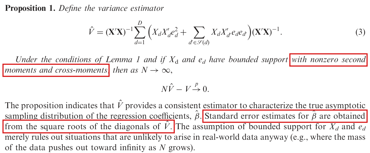
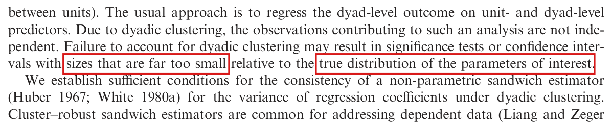
The stated conditions allow a coefficient whose limiting variance is zero, for which the variance estimate can be negative; the claim of valid confidence intervals and tests needs a positive limiting variance for each tested contrast and a central limit theorem.

Proposition 1 and the two sentences after it, p. 567 (PDF p. 4); the conditions before Lemma 1, p. 566 (PDF p. 3); Section 1, p. 565 (PDF p. 2); Section 5, p. 571 (PDF p. 8)

See also under Formal statements (Lean): P018-T7, P018-T8

As printed

p. 567: “Under the conditions of Lemma 1 and if XdX_{\mathrm{d}} and ede_d have bounded support with nonzero second moments and cross-moments, then as N→∞N\to\infty,

NV^−V→p0.N\hat V-V\overset{p}{\to}0.

The proposition indicates that V^\hat V provides a consistent estimator to characterize the true asymptotic sampling distribution of the regression coefficients, β^\hat\beta. Standard error estimates for β^\hat\beta are obtained from the square roots of the diagonals of V^\hat V.”

p. 565: “Second, Erikson, Pinto, and Rader’s (2014) solution of non-parametric randomization inference does not provide a procedure for obtaining valid confidence intervals, while our procedure does.”

The problem

Lemma 1 states the mean and the variance of the limit of N(β^−β)\sqrt{N}(\hat\beta-\beta), and by Proposition 1 the difference NV^−VN\hat V-V converges to zero in probability. Neither statement excludes a coefficient, or a linear combination c′βc'\beta of coefficients, whose limiting variance is zero. For such a contrast the proposition says only that Nc′V^cNc'\hat Vc converges to zero. It does not say that c′V^cc'\hat Vc is positive, or that the ratio of c′(β^−β)c'(\hat\beta-\beta) to c′V^c\sqrt{c'\hat Vc} is approximately standard normal. The rank conditions on X\mathbf{X} and the condition of “nonzero second moments and cross-moments” do not exclude this case: in the example below every entry of the matrices of second moments and cross-moments is nonzero, and the limiting variance of the slope is zero. The paper also states no central limit theorem for the score sum, and a confidence interval based on the normal distribution needs one. The conditions as stated are not sufficient for the claim of valid confidence intervals on p. 565, for the standard errors prescribed after Proposition 1, or for the test in Section 5.

Evidence an exact counterexample

The evidence is an exact counterexample and a derivation. For each unit ii let ZiZ_i and WiW_i be independent signs, each equal to ±1\pm1 with probability 1/21/2, and for i<ji<j set Xij=(1, 1+ZiZj)′X_{ij}=(1,\,1+Z_iZ_j)' and Yij=Wi+WjY_{ij}=W_i+W_j. The data and the fitted residuals are bounded, and, for N≥3N\ge3, the design matrix has full rank whenever both signs of ZZ occur. The population coefficient is β=(0,0)′\beta=(0,0)', and ϵij=Yij\epsilon_{ij}=Y_{ij}. I have E[XijXij′ϵij2]=2Q\mathrm{E}[X_{ij}X_{ij}'\epsilon_{ij}^2]=2Q, where

Q=E[XijXij′]=(1112),Ω=E[XijXik′ϵijϵik]=(1111),Q=\mathrm{E}[X_{ij}X_{ij}']=\begin{pmatrix}1&1\\1&2\end{pmatrix},\qquad\Omega=\mathrm{E}[X_{ij}X_{ik}'\epsilon_{ij}\epsilon_{ik}]=\begin{pmatrix}1&1\\1&1\end{pmatrix},

and every entry of these matrices is nonzero. By equation (1), I have

V=ND2 Q−1{2DQ+N(N−1)(N−2)Ω}Q−1→4Q−1ΩQ−1=(4000),V=\frac{N}{D^2}\,Q^{-1}\{2DQ+N(N-1)(N-2)\Omega\}Q^{-1}\to4Q^{-1}\Omega Q^{-1}=\begin{pmatrix}4&0\\0&0\end{pmatrix},

and the slope entry of VV is 4/(N−1)4/(N-1). I take eight units with (Zi,Wi)(Z_i,W_i) equal to (1,1)(1,1), (1,−1)(1,-1), (−1,1)(-1,1), (−1,−1)(-1,-1), each twice. Then β^=0\hat\beta=0, and the estimator (3) is

V^=(3/8−1/48−1/48−13/288).\hat V=\begin{pmatrix}3/8&-1/48\\-1/48&-13/288\end{pmatrix}.

The estimated variance of the slope is −13/288-13/288, and its standard error is not defined. This is not an accident of one sample. Let β^1\hat\beta_1 denote the slope estimate and V^22\hat V_{22} its estimated variance. As N→∞N\to\infty, the pair (Nβ^1,N2V^22)(N\hat\beta_1,N^2\hat V_{22}) converges in distribution to (2AB, 4(A2+B2−1))(2AB,\,4(A^2+B^2-1)), where AA and BB are independent standard normal variables. The probability that V^22\hat V_{22} is negative therefore converges to Pr⁡(A2+B2<1)=1−e−1/2\Pr(A^2+B^2<1)=1-e^{-1/2}, about 0.3930.393. In the same example NV^N\hat V converges in probability to diag⁡(4,0)\operatorname{diag}(4,0), which agrees with Proposition 1.

For the repair, let UiU_i denote the characteristics of unit ii, write s(Ui,Uj)=Xd(i,j)ϵd(i,j)s(U_i,U_j)=X_{d(i,j)}\epsilon_{d(i,j)}, and set η(u)=E[s(u,Uj)]\eta(u)=\mathrm{E}[s(u,U_j)] and r(u,v)=s(u,v)−η(u)−η(v)r(u,v)=s(u,v)-\eta(u)-\eta(v). Then E[η(Ui)]=0\mathrm{E}[\eta(U_i)]=0 and E[r(Ui,Uj)∣Ui]=0\mathrm{E}[r(U_i,U_j)\mid U_i]=0, and

1D∑i<js(Ui,Uj)=2N∑i=1Nη(Ui)+1D∑i<jr(Ui,Uj).\frac{1}{D}\sum_{i<j}s(U_i,U_j)=\frac{2}{N}\sum_{i=1}^{N}\eta(U_i)+\frac{1}{D}\sum_{i<j}r(U_i,U_j).

Distinct terms of the last sum are uncorrelated, and its covariance matrix is E[rr′]/D\mathrm{E}[rr']/D, of order N−2N^{-2}. The vectors η(Ui)\eta(U_i) are i.i.d., bounded and of mean zero, with covariance matrix Ω=E[Xd(i,j)Xd(i,k)′ϵd(i,j)ϵd(i,k)]\Omega=\mathrm{E}[X_{d(i,j)}X_{d(i,k)}'\epsilon_{d(i,j)}\epsilon_{d(i,k)}], and D−1∑dXdXd′D^{-1}\sum_dX_dX_d' converges in probability to Q=E[XdXd′]Q=\mathrm{E}[X_dX_d']. By the central limit theorem for i.i.d. vectors and Slutsky’s theorem, I obtain that N(β^−β)\sqrt{N}(\hat\beta-\beta) converges in distribution to a normal vector with mean zero and covariance matrix V∞=4Q−1ΩQ−1V_\infty=4Q^{-1}\Omega Q^{-1}, which is also the limit of VV. If c′V∞c>0c'V_\infty c>0, then Proposition 1 implies that Nc′V^cNc'\hat Vc converges in probability to c′V∞cc'V_\infty c, and I conclude by Slutsky’s theorem that the ratio has a standard normal limit.

What survives

Lemma 1 as a statement of mean and variance and the conclusion NV^−V→p0N\hat V-V\overset{p}{\to}0 of Proposition 1 are not contradicted; both hold in the example. Proposition 2, the computation of the estimator and every reported coefficient and standard error are unaffected, and the limiting variance in the simulation design of Section 4 is positive definite. What changes is the scope of the claims about confidence intervals and tests, which hold for contrasts whose limiting variance is positive. I have not checked this condition for the two applications. The corresponding condition is needed for repeated observations and for generalized linear models.

Corrected

Proposition 1 stands. Add after it: “Let Q=E[XdXd′]Q=\mathrm{E}[X_dX_d'], let Ω=E[Xd(i,j)Xd(i,k)′ϵd(i,j)ϵd(i,k)]\Omega=\mathrm{E}[X_{d(i,j)}X_{d(i,k)}'\epsilon_{d(i,j)}\epsilon_{d(i,k)}] for distinct units ii, jj, kk, and let V∞=4Q−1ΩQ−1V_\infty=4Q^{-1}\Omega Q^{-1}. Under the conditions of Lemma 1 (a random (i.i.d.) sample of units, XdX_d and YdY_d with support bounded in a finite interval, and the usual rank conditions on X\mathbf{X}), N(β^−β)\sqrt{N}(\hat\beta-\beta) converges in distribution to a normal vector with mean zero and covariance matrix V∞V_\infty, which may be singular. Let cc be a fixed vector such that c′V∞c>0c'V_\infty c>0. Then, under the conditions of Proposition 1,

c′(β^−β)c′V^c→dN(0,1)as N→∞.\frac{c'(\hat\beta-\beta)}{\sqrt{c'\hat Vc}}\overset{d}{\to}N(0,1)\qquad\text{as }N\to\infty.

In particular, the standard error of β^k\hat\beta_k, the square root of the kkth diagonal entry of V^\hat V, supports a normal confidence interval or test when the kkth diagonal entry of V∞V_\infty is positive.”

p. 565: “… does not provide a procedure for obtaining valid confidence intervals, while our procedure does for coefficients and contrasts whose limiting variance is positive.”

Crop of Proposition 1: the estimator of equation (3), the sentence 'Under the conditions of Lemma 1 and if X_d and e_d have bounded support with nonzero second moments and cross-moments, then as N goes to infinity', the display 'N V-hat minus V converges in probability to 0', and five lines of the next paragraph. Red boxes mark 'with nonzero second moments and cross-moments' and 'Standard error estimates for beta-hat are obtained from the square roots of the diagonals of V-hat.'
Proposition 1 and the paragraph after it, p. 567 (PDF p. 4). The marks are on the condition “with nonzero second moments and cross-moments” and on the sentence that prescribes the standard errors.
Crop of six lines from the introduction on page 565. A red box marks 'valid confidence intervals, while our procedure does.' in the sentence 'Second, Erikson, Pinto, and Rader's (2014) solution of non-parametric randomization inference does not provide a procedure for obtaining valid confidence intervals, while our procedure does.'
Section 1, p. 565 (PDF p. 2). The mark is on the claim of valid confidence intervals.

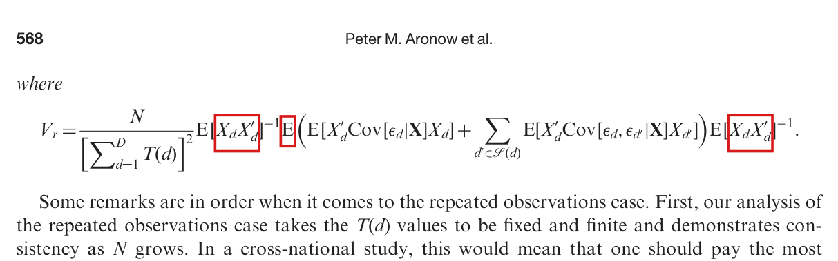
The limits VrV_r and VwV_w need a sum over dyads in the middle factor, where an expectation is printed, and normalised k×kk \times k Gram matrices in the outer factors.

Display that defines VrV_r after Corollary 1, p. 568 (PDF p. 5, top); display that defines VwV_w after Corollary 2, p. 576 (PDF p. 13, top)

See also under Formal statements (Lean): P018-T10, P018-T11, P018-T12, P018-T28

As printed
Vr=N[∑d=1DT(d)]2 E⁡[XdXd′]−1 E⁡(E⁡[Xd′Cov⁡[ϵd∣X]Xd]+∑d′∈S(d)E⁡[Xd′Cov⁡[ϵd,ϵd′∣X]Xd′])E⁡[XdXd′]−1.\begin{aligned} V_r = {}& \frac{N}{\bigl[\sum_{d=1}^{D} T(d)\bigr]^{2}}\, \operatorname{E}[\colorbox{#ffe58a}{$\displaystyle X_d X_d'$}]^{-1}\, \colorbox{#ffe58a}{$\displaystyle \operatorname{E}$} \Bigl( \operatorname{E}[X_d' \operatorname{Cov}[\epsilon_d | \mathbf{X}] X_d] \\ & + \sum_{d' \in \mathcal{S}(d)} \operatorname{E}[X_d' \operatorname{Cov}[\epsilon_d, \epsilon_{d'} | \mathbf{X}] X_{d'}] \Bigr) \operatorname{E}[\colorbox{#ffe58a}{$\displaystyle X_d X_d'$}]^{-1}. \end{aligned}
Vw=ND2 E⁡[wdXd′Xd]−1 E⁡(E⁡[XdXd′wd2Var⁡[ϵd∣X]]+∑d′∈S(d)E⁡[XdXd′′wdwd′Cov⁡[ϵd,ϵd′∣X]])E⁡[wdXdXd′]−1.\begin{aligned} V_w = {}& \frac{N}{D^{2}}\, \operatorname{E}[w_d \colorbox{#ffe58a}{$\displaystyle X_d' X_d$}]^{-1}\, \colorbox{#ffe58a}{$\displaystyle \operatorname{E}$} \Bigl( \operatorname{E}\bigl[X_d X_d' w_d^2 \operatorname{Var}[\epsilon_d | \mathbf{X}]\bigr] \\ & + \sum_{d' \in \mathcal{S}(d)} \operatorname{E}\bigl[X_d X_{d'}' w_d w_{d'} \operatorname{Cov}[\epsilon_d, \epsilon_{d'} | \mathbf{X}]\bigr] \Bigr) \operatorname{E}[w_d X_d X_d']^{-1}. \end{aligned}
The problem

Both displays print an outer expectation of the bracket for a single dyad dd, where equations (1) and (2) have a sum over dd. In the example below, both printed limits equal 4/D4/D and tend to zero, while NVar⁡[β^]N\operatorname{Var}[\widehat\beta] equals 44. Both conclusions of each corollary then fail with the printed definitions. The outer factors do not conform either. In the repeated dyads case, XdX_d is the T(d)×kT(d) \times k matrix with rows Xdt′X_{dt}', and XdXd′X_d X_d' is a T(d)×T(d)T(d) \times T(d) matrix, whose size varies with dd. In the weighted case, the left factor E⁡[wdXd′Xd]−1\operatorname{E}[w_d X_d' X_d]^{-1} is the inverse of a scalar, and the right factor is the inverse of a k×kk \times k matrix. For VrV_r it is not enough to restore the sum and to write Xd′XdX_d' X_d. The prefactor counts observations, through ∑dT(d)\sum_d T(d), and the Gram matrix must be normalised by the same count.

Evidence an exact counterexample

The evidence is an exact counterexample with a derivation. Let U1,…,UNU_1, \dots, U_N be independent signs, each equal to ±1\pm 1 with probability 1/21/2, and for each dyad set Xij=1X_{ij} = 1 and Yij=Ui+UjY_{ij} = U_i + U_j, with T(d)=1T(d) = 1 and wd=1w_d = 1. The population coefficient is β=0\beta = 0, and ϵij=Ui+Uj\epsilon_{ij} = U_i + U_j. Each unit belongs to N−1N - 1 dyads, so β^=(2/N)∑iUi\widehat\beta = (2/N) \sum_i U_i, and

NVar⁡[β^−β]=4.N \operatorname{Var}[\widehat\beta - \beta] = 4.

A dyad has residual variance 22 and covariance 11 with each of the 2(N−2)2(N-2) dyads that share a member with it. The printed bracket equals 2+2(N−2)=2N−22 + 2(N - 2) = 2N - 2 for every dd, and

Vrprinted=Vwprinted=N(2N−2)D2=4D.V_r^{\text{printed}} = V_w^{\text{printed}} = \frac{N(2N - 2)}{D^2} = \frac{4}{D}.

With the sum over dyads restored, the middle factor is D(2N−2)=N(N−1)2D(2N - 2) = N(N-1)^2, and the limit is (N/D2) N(N−1)2=4(N/D^2)\, N(N-1)^2 = 4.

The example Xij=1X_{ij} = 1, Yij=Ui+UjY_{ij} = U_i + U_j: exact values for four sample sizes.
NNDDNVar⁡[β^]N\operatorname{Var}[\widehat\beta]VrV_r and VwV_w as printedVrV_r and VwV_w as corrected
3333444/34/344
4466442/32/344
551010442/52/544
10104545444/454/4544

Note that the estimators carry the sum over dyads. In this example NV^r=NV^wN\widehat V_r = N\widehat V_w converges to 44 in probability. For the outer factors, suppose that each observation of the example is repeated twice, so that T(d)=2T(d) = 2 and Xd=(1,1)′X_d = (1, 1)'. Then

E⁡[XdXd′]=(1111)\operatorname{E}[X_d X_d'] = \begin{pmatrix} 1 & 1 \\ 1 & 1 \end{pmatrix}

is singular, while E⁡[Xd′Xd]=2\operatorname{E}[X_d' X_d] = 2. Restoring the sum and writing Xd′XdX_d' X_d, with no other change, I find the value 11. The normalised matrix HrH_r below gives 44.

The form of the corrected displays comes from the identity

N(β^r−βr)=(X′XL)−1NL∑d=1DXd′ϵd,\sqrt{N}(\widehat\beta_r - \beta_r) = \Bigl(\frac{\mathbf{X}'\mathbf{X}}{L}\Bigr)^{-1} \frac{\sqrt{N}}{L} \sum_{d=1}^{D} X_d' \epsilon_d,

where L=∑dT(d)L = \sum_d T(d). Replacing X′X/L\mathbf{X}'\mathbf{X}/L by its population version HrH_r, I obtain a vector with covariance matrix (N/L2)Hr−1ΩrHr−1(N/L^2) H_r^{-1} \Omega_r H_r^{-1}. The weighted case is the same, with X′WX/D\mathbf{X}'\mathbf{W}\mathbf{X}/D, DD and ∑dwdXdϵd\sum_d w_d X_d \epsilon_d.

What survives

The estimators V^r\widehat V_r on p. 567 and V^w\widehat V_w in equation (7), equation (1), Proposition 2 and Appendix C do not use these displays. The replication scripts compute the sandwich through the decomposition of Proposition 2, in the repeated-observations simulation and in both applications, and no reported number changes. The corrected displays define the population covariance targets at sample size NN; their limits, when they exist, are the asymptotic covariance matrices. They are not a proof of the two corollaries. The middle factor is written below as the variance of the total score, as in equation (1). The conditional form of the printed middle factor is the subject of P018-E001.

Corrected

For the repeated dyads case, let XdX_d be the T(d)×kT(d) \times k matrix with rows Xdt′X_{dt}', and let ϵd\epsilon_d be the vector of the T(d)T(d) population residuals of dyad dd. Write L=∑d=1DT(d)L = \sum_{d=1}^{D} T(d), and define

Hr=1L∑d=1DE⁡[Xd′Xd],Ωr=Var⁡[∑d=1DXd′ϵd].H_r = \frac{1}{L} \sum_{d=1}^{D} \operatorname{E}[X_d' X_d], \qquad \Omega_r = \operatorname{Var}\Bigl[\sum_{d=1}^{D} X_d' \epsilon_d\Bigr].

Then

Vr=NL2 Hr−1 Ωr Hr−1.V_r = \frac{N}{L^{2}}\, \colorbox{#ffe58a}{$\displaystyle H_r^{-1}\, \Omega_r\, H_r^{-1}$}.

For the weighted dyads case, let XdX_d be the kk-vector of regressors of dyad dd, and define

Hw=1D∑d=1DE⁡[wdXdXd′],Ωw=Var⁡[∑d=1DwdXdϵd].H_w = \frac{1}{D} \sum_{d=1}^{D} \operatorname{E}[w_d X_d X_d'], \qquad \Omega_w = \operatorname{Var}\Bigl[\sum_{d=1}^{D} w_d X_d \epsilon_d\Bigr].

Then

Vw=ND2 Hw−1 Ωw Hw−1.V_w = \frac{N}{D^{2}}\, \colorbox{#ffe58a}{$\displaystyle H_w^{-1}\, \Omega_w\, H_w^{-1}$}.
Crop of the top of p. 568, with the running head 568, Peter M. Aronow et al. The word where is followed by a display: V r equals N over the square of the sum over d from 1 to D of T of d, times the inverse of E of X d times X d transposed, times E of a large bracket, times the inverse of E of X d times X d transposed. The bracket holds E of X d transposed times Cov of epsilon d given X times X d, plus the sum over d-prime in S of d of E of X d transposed times Cov of epsilon d and epsilon d-prime given X times X d-prime. Three red outlines surround the product X d times X d transposed in the left factor, the letter E in front of the large bracket, and the product X d times X d transposed in the right factor. The first lines of the next paragraph follow.
Top of p. 568 (PDF p. 5): the display that defines VrV_r. The outlines mark the product XdXd′X_d X_d' in both outer factors and the outer expectation E of the middle factor.
Crop of one display introduced by the word where: V w equals N over D squared, times the inverse of E of w d times X d transposed times X d, times E of a large bracket, times the inverse of E of w d times X d times X d transposed. The bracket holds E of X d times X d transposed times w d squared times Var of epsilon d given X, plus the sum over d-prime in S of d of E of X d times X d-prime transposed times w d w d-prime times Cov of epsilon d and epsilon d-prime given X. Two red outlines surround the product X d transposed times X d in the left factor and the letter E in front of the large bracket.
Top of p. 576 (PDF p. 13): the display that defines VwV_w. The outlines mark the scalar product Xd′XdX_d' X_d in the left factor and the outer expectation E.

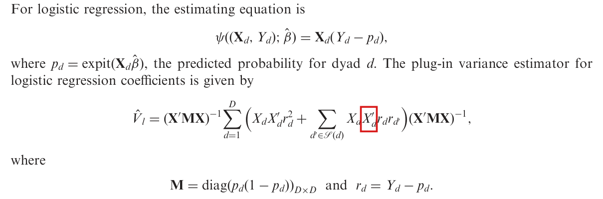
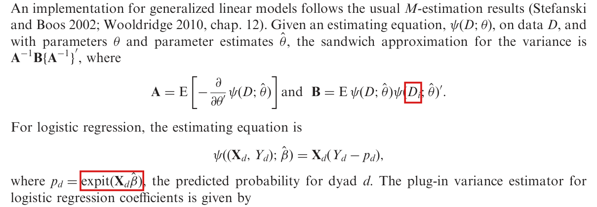
In the plug-in variance estimator for logistic regression of Appendix E, the cross-dyad term is XdXd′′rdrd′X_dX_{d'}'r_dr_{d'}, which pairs the regressors of both dyads, and not XdXd′rdrd′X_dX_d'r_dr_{d'}.

Appendix E, p. 576 (PDF p. 13), display of the plug-in variance estimator V^l\hat V_l, cross-dyad term

See also under Formal statements (Lean): P018-T13, P018-T14

As printed

The plug-in variance estimator for logistic regression coefficients is given by

V^l=(X′MX)−1∑d=1D(XdXd′rd2+∑d′∈S(d)XdXd′rdrd′)(X′MX)−1,\hat V_l=(\mathbf X'\mathbf M\mathbf X)^{-1}\sum_{d=1}^{D}\Big(X_dX_d'r_d^2+\sum_{d'\in\mathcal S(d)}X_dX_{\colorbox{#ffe58a}{$\displaystyle d$}}'r_dr_{d'}\Big)(\mathbf X'\mathbf M\mathbf X)^{-1},

where M=diag⁡(pd(1−pd))D×D\mathbf M=\operatorname{diag}(p_d(1-p_d))_{D\times D} and rd=Yd−pdr_d=Y_d-p_d.

The problem

The estimating function printed just above the display is the score Xd(Yd−pd)=XdrdX_d(Y_d-p_d)=X_dr_d. The sandwich sums the products of the scores of dyads that share a unit, and the product of the scores of dd and d′d' is XdXd′′rdrd′X_dX_{d'}'r_dr_{d'}, as in equations (3) and (7). The printed cross term repeats XdX_d where Xd′X_{d'} belongs. A computation that follows the display literally gives a different matrix.

Evidence an exact counterexample

The evidence is an exact example. Let the six dyads of four units be ordered as {1,2}\{1,2\}, {1,3}\{1,3\}, {1,4}\{1,4\}, {2,3}\{2,3\}, {2,4}\{2,4\}, {3,4}\{3,4\}, and let Xd=(1,xd)′X_d=(1,x_d)' with x=(0,2,5,5,1,1)x=(0,2,5,5,1,1) and Y=(1,1,1,0,0,0)Y=(1,1,1,0,0,0). The score vanishes at β^=(0,0)′\hat\beta=(0,0)'. Since the design has rank two, the log-likelihood is strictly concave, and this point is the maximum likelihood estimate. At this estimate, I have pd=1/2p_d=1/2, rd=±1/2r_d=\pm1/2 and

X′MX=(3/27/27/214).\mathbf X'\mathbf M\mathbf X=\begin{pmatrix}3/2&7/2\\7/2&14\end{pmatrix}.

With the cross term XdXd′′rdrd′X_dX_{d'}'r_dr_{d'} and with the printed cross term, I obtain respectively

(38/25−64/175−64/175192/1225)and(8/5−2/5−2/56/35).\begin{pmatrix}38/25&-64/175\\-64/175&192/1225\end{pmatrix}\qquad\text{and}\qquad\begin{pmatrix}8/5&-2/5\\-2/5&6/35\end{pmatrix}.

The first matrix agrees with the computation from sums of scores by unit, less the dyad terms, which is the form that the authors' code uses. A recalculation with that code from the replication data reproduces the nine coefficients of the pooled logistic regression in Table 1 and their dyadic standard errors to three decimals.

What survives

The authors' code forms products of scores and does not contain the misprint. Table 1 and the conclusion about the coefficient for international organizations are unchanged. The formulas for linear regression do not use this display. The other notation of Appendix E is corrected in P018-N010.

Corrected

The plug-in variance estimator for logistic regression coefficients is given by

V^l=(X′MX)−1∑d=1D(XdXd′rd2+∑d′∈S(d)XdXd′′rdrd′)(X′MX)−1,\hat V_l=(\mathbf X'\mathbf M\mathbf X)^{-1}\sum_{d=1}^{D}\Big(X_dX_d'r_d^2+\sum_{d'\in\mathcal S(d)}X_dX_{\colorbox{#ffe58a}{$\displaystyle d'$}}'r_dr_{d'}\Big)(\mathbf X'\mathbf M\mathbf X)^{-1},

where M=diag⁡(pd(1−pd))D×D\mathbf M=\operatorname{diag}(p_d(1-p_d))_{D\times D}, rd=Yd−pdr_d=Y_d-p_d, pd=expit⁡(Xd′β^)p_d=\operatorname{expit}(X_d'\hat\beta), and S(d)\mathcal S(d) is the set of dyads other than dd that share a member with dd.

Crop of the logistic estimating equation, the definition of p d, the display of the estimator V hat l, and the definitions of M and r d. A red box marks the second regressor in the cross-dyad term, X prime with subscript d, where the subscript d prime belongs.
Appendix E, p. 576 (PDF p. 13), display of V^l\hat V_l. The marked second regressor of the cross term has the subscript dd; the residual beside it has the subscript d′d'.

The sum over the dyads that do not contain unit ii runs over j<kj < k with j,k≠ij, k \ne i, so that each such dyad is counted once.

Proposition 2, definition of Σ^C,i\widehat\Sigma_{C,i}, p. 568 (PDF p. 5); the same index in EiE_i, Appendix C, p. 575 (PDF p. 12)

See also under Formal statements (Lean): P018-T15, P018-T16

As printed
Σ^C,i=∑j≠i∑k≠iXd(i,j)′ed(i,j)ed(i,k)′Xd(i,k)+∑j,k≠i∑t=1T(d(j,k))Xd(j,k)tXd(j,k)t′ed(j,k)t2,\widehat\Sigma_{C,i} = \sum_{j \ne i} \sum_{k \ne i} X_{d(i,j)}' e_{d(i,j)} e_{d(i,k)}' X_{d(i,k)} + \sum_{\colorbox{#ffe58a}{$\displaystyle j,k \ne i$}} \sum_{t=1}^{T(d(j,k))} X_{d(j,k)t} X_{d(j,k)t}' e_{d(j,k)t}^{2},

and, in Appendix C,

Ei=∑j,k≠i∑t=1T(d(j,k))Xd(j,k)tXd(j,k)t′ed(j,k)t2.E_i = \sum_{\colorbox{#ffe58a}{$\displaystyle j,k \ne i$}} \sum_{t=1}^{T(d(j,k))} X_{d(j,k)t} X_{d(j,k)t}' e_{d(j,k)t}^{2}.
The problem

The index j,k≠ij, k \ne i carries neither j<kj < k nor j≠kj \ne k. The first double sum of the same display runs over ordered pairs. Read in the same way, the second sum includes the dyads d(j,j)d(j,j), which the paper excludes, and counts every other dyad twice, since d(j,k)=d(k,j)d(j,k) = d(k,j). The identity (N−2)Σ^0=∑iEi(N-2)\widehat\Sigma_0 = \sum_i E_i of Appendix C then fails by a factor of 22. The sentence below Proposition 2 and the count in Appendix C show that each dyad without unit ii is meant to enter once.

Evidence a derivation

The evidence is a derivation by counting, with an exact example. A dyad avoids exactly N−2N - 2 units. If each dyad without unit ii enters EiE_i once, then ∑iEi=(N−2)Σ^0\sum_i E_i = (N-2)\widehat\Sigma_0, and ∑iΣ^C,i−Σ^D−(N−2)Σ^0\sum_i \widehat\Sigma_{C,i} - \widehat\Sigma_D - (N-2)\widehat\Sigma_0 equals the middle factor of V^r\widehat V_r. If each enters twice, then ∑iEi=2(N−2)Σ^0\sum_i E_i = 2(N-2)\widehat\Sigma_0. For N=4N = 4, one observation per dyad and scalar scores Xded=1,2,…,6X_d e_d = 1, 2, \dots, 6, I have Σ^0=91\widehat\Sigma_0 = 91, and the middle factor of V^r\widehat V_r, computed directly from its definition, is 385385. Counting each dyad once, I find ∑iEi=182\sum_i E_i = 182, and the decomposition returns 385385. Counting each dyad twice gives ∑iEi=364\sum_i E_i = 364, and the decomposition returns 567567. The replication script assigns each observation without unit ii to its own cluster, which counts each dyad once.

What survives

Proposition 2 and the identities of Appendix C hold with the index as corrected. The replication code and every reported number are unaffected.

Corrected
Σ^C,i=∑j≠i∑k≠iXd(i,j)′ed(i,j)ed(i,k)′Xd(i,k)+∑j<kj,k≠i∑t=1T(d(j,k))Xd(j,k)tXd(j,k)t′ed(j,k)t2,\widehat\Sigma_{C,i} = \sum_{j \ne i} \sum_{k \ne i} X_{d(i,j)}' e_{d(i,j)} e_{d(i,k)}' X_{d(i,k)} + \sum_{\substack{\colorbox{#ffe58a}{$\displaystyle j < k$} \\ j, k \ne i}} \sum_{t=1}^{T(d(j,k))} X_{d(j,k)t} X_{d(j,k)t}' e_{d(j,k)t}^{2},

and, in Appendix C,

Ei=∑j<kj,k≠i∑t=1T(d(j,k))Xd(j,k)tXd(j,k)t′ed(j,k)t2.E_i = \sum_{\substack{\colorbox{#ffe58a}{$\displaystyle j < k$} \\ j, k \ne i}} \sum_{t=1}^{T(d(j,k))} X_{d(j,k)t} X_{d(j,k)t}' e_{d(j,k)t}^{2}.
Crop of two displays that follow the word and. The first defines Sigma-hat C,i as the sum over j not equal to i and over k not equal to i of X d(i,j) transposed times e d(i,j) times e d(i,k) transposed times X d(i,k), plus a sum indexed by j, k not equal to i of the sum over t from 1 to T of d(j,k) of X d(j,k)t times X d(j,k)t transposed times e d(j,k)t squared. The second defines Sigma-hat D and Sigma-hat 0. A red outline surrounds the index j, k not equal to i under the third summation sign. The first line of the next paragraph follows.
Proposition 2, p. 568 (PDF p. 5): the definition of Σ^C,i\widehat\Sigma_{C,i}. The outline marks the index j,k≠ij, k \ne i of the sum over the dyads that do not contain unit ii.
Crop of one display introduced by the word Define: D i equals the sum over j not equal to i of X d(i,j) transposed times e d(i,j) times e d(i,j) transposed times X d(i,j), and E i equals a sum indexed by j, k not equal to i of the sum over t from 1 to T of d(j,k) of X d(j,k)t times X d(j,k)t transposed times e d(j,k)t squared. A red outline surrounds the index j, k not equal to i under the first summation sign of E i. The next line reads: Then, working with Sigma-hat C,i, Sigma-hat D, and Sigma-hat 0 as defined in the proposition.
Appendix C, p. 575 (PDF p. 12): the definition of EiE_i. The outline marks the same index j,k≠ij, k \ne i.

The blue curve in Figure 4 of the Supporting Information is a quadratic least-squares fit to the plotted sample, not the true conditional mean x+0.25x2x+0.25x^2.

Supporting Information, Figure 4 and its caption, p. 3 (supplement PDF p. 3); the sentence beginning “Figure 4 shows”, p. 4 (supplement PDF p. 4)

As printed

Supporting Information, p. 3: “Figure 4: Illustrative scatter plot and linear approximation for the misspecification case. The blue line is the true conditional mean, and the red line is the linear approximation.”

Supporting Information, p. 4: “Figure 4 shows the scatter plot of Yd(i,j)tY_{d(i,j)t} against ∣Xi−Xj∣|X_i-X_j|, the linear approximation (in red) for one of the simulation replicates (N=50N=50), and the true conditional mean (in blue).”

The problem

Let x=∣Xi−Xj∣x=|X_i-X_j|. In the design of the Supporting Information, β0=0\beta_0=0, β1=1\beta_1=1 and β2=0.25\beta_2=0.25, and the shocks have mean zero and are independent of the covariates, so that the conditional mean of YY given xx is x+0.25x2x+0.25x^2. The plotting script in the replication files draws the blue curve as the fitted values of a least-squares regression of the simulated outcomes on xx and x2x^2 with an intercept. Its three coefficients are estimates from the one sample plotted, and with probability one they differ from (0,1,0.25)(0,1,0.25).

Evidence an exact counterexample

The evidence is a check of the script and an exact comparison with the published figure. Line 437 of the graph script draws the blue curve from the values predict(lm(dY.ord∼\simdX.ord+I(dX.ord^\text{\textasciicircum}2))). In the published PDF, the coordinates of the blue curve and of the axis ticks place its right end at x≈3.363x\approx3.363 and height 7.2477.247, where x+0.25x2≈6.191x+0.25x^2\approx6.191. The gap of about 1.061.06 stays above 1 when the rounding of the coordinates is allowed for.

What survives

The figure is an illustration, and the fitted curve enters no number. The design, the simulation summaries in Figure 3 of the Supporting Information and the conclusions drawn from them are unaffected.

Corrected

Caption: “… The blue line is a quadratic least-squares fit to the plotted sample, and the red line is the linear least-squares fit.”

p. 4: “… the linear approximation (in red) for one of the simulation replicates (N=50N=50), and a quadratic least-squares fit to that sample (in blue).”

Alternatively, the label can stay if the figure is drawn again with the curve x+0.25x2x+0.25x^2 in blue.

Crop of Figure 4 of the Supporting Information: a scatter plot of Y against the absolute difference of X_i and X_j, which runs from 0 to about 3.4, with a red straight line and a blue curve that bends upward and ends near height 7.2. Below the plot is the caption 'Figure 4: Illustrative scatter plot and linear approximation for the misspecification case. The blue line is the true conditional mean, and the red line is the linear approximation.' Red boxes mark 'The blue line is the true conditional mean,'.
Supporting Information, Figure 4 and its caption, p. 3. The marks are on the part of the caption that calls the blue line the true conditional mean.
Crop of seven lines of text from page 4 of the Supporting Information. A red box marks 'and the true conditional mean (in blue).' in the sentence 'Figure 4 shows the scatter plot of Y against the absolute difference of X_i and X_j, the linear approximation (in red) for one of the simulation replicates (N = 50), and the true conditional mean (in blue).'
Supporting Information, p. 4. The mark is on “and the true conditional mean (in blue)”.

The pooled logistic columns of Table 1 use 39,996 observations in 1,186 dyads, not 39,988 and 1,178. A processed copy of the speed-dating data reproduces Table 2 of the Supporting Information with 268 women, against the printed 278; this count remains unconfirmed against the authors' raw file.

Note to Table 1, p. 572 (PDF p. 9); Section 5, second paragraph, p. 571 (PDF p. 8); Supporting Information, p. 5, first paragraph and note to Table 2

As printed

P. 571: They use annual data on 146 states in the international system paired into 1178 dyads (out of 10,585 possible) and observed for as few as one and as many as 90 years between 1885 and 1991, for a total of 39,988 observations.

Table 1, p. 572: Note: N=39,988N=\colorbox{#ffe58a}{$39{,}988$} dyad–year observations for 1,178 dyads and 146 units.

Supporting Information, p. 5: These data include 278 women paired into 3,457 female-male dyads. […] N=3,457N=3{,}457 dyad observations for 278 subjects.

The problem

The note stands under the whole of Table 1 and gives no separate counts for columns (3)–(6). The replication data hold 39,996 complete dyad-years in 1,186 dyads among 146 states, with 1 to 90 observations per dyad. The pooled logistic regression on all of them reproduces every coefficient in column (3) and every dyadic standard error in column (6). The printed counts 39,988 and 1,178 are what remains when the eight dyads with a single observation are removed. That smaller sample has 145 states and 2 to 90 observations per dyad, and several of its coefficients do not round to the printed ones: for lower dependence it gives −67.733-67.733 against the printed −67.668-67.668. Neither sample has all four properties stated on p. 571.

In the Supporting Information, the sample of 3,457 dyads that reproduces Table 2 has 268 women and 277 men.

Evidence a recalculation from the source

I recalculated the sample counts from the replication data; they are exact.

The two samples in the replication data for Table 1, and the printed description.
SampleObservationsDyadsStatesObservations per dyad
All complete dyad-years39,9961,1861461 to 90
Without the eight single-observation dyads39,9881,1781452 to 90
As printed (p. 571 and note to Table 1)39,9881,1781461 to 90

The count of 268 women comes from a processed copy of the speed-dating data that is distributed with an R package by other authors. With the fixed effects and weights of the authors' script, this copy reproduces all 12 entries of Table 2 to four decimals. I did not use the authors' raw data file, and I have not confirmed the count of 268 against that file.

I have not established which sample the GEE of columns (1)–(2) used. Since an AR(1) working correlation is defined for a dyad with one observation, the model alone does not require that these dyads be dropped. My GEE calculations on the smaller sample approximate columns (1)–(2), but do not reproduce every entry to the printed rounding or establish that this was the GEE sample. The original Stata run was not repeated.

What survives

The nine coefficients of the pooled logistic regression in Table 1 and their dyadic standard errors are reproduced unchanged, and the test statistic for international organizations is 1.311.31, below the threshold 1.641.64. All 12 entries of Table 2 of the Supporting Information are reproduced. No theorem, formula or simulation depends on these counts. Only the descriptions of the samples change.

Corrected

Note to Table 1: columns (3)–(6) use N=39,996N=\colorbox{#ffe58a}{$39{,}996$} dyad–year observations for 1,186 dyads and 146 units, with 1 to 90 observations per dyad. If the GEE of columns (1)–(2) excludes the eight dyads with a single observation, its sample has N=39,988N=39{,}988 observations for 1,178 dyads and 145 units, with 2 to 90 observations per dyad; this is to be confirmed from the estimation sample.

Supporting Information, p. 5: These data include 268 women paired into 3,457 female-male dyads. […] N=3,457N=3{,}457 dyad observations for 268 subjects. This count is to be confirmed against the authors' raw data file before the text is changed.

Crop of Table 1 without its title: nine rows of coefficients and standard errors in six columns, the first two headed Original GEE estimates and the last four Simple logistic regression estimates. In the note below the table, red boxes mark the numbers 39,988 and 1,178.
Table 1, p. 572 (PDF p. 9). The marked counts in the note stand under all six columns; columns (3)–(6) are computed from 39,996 observations in 1,186 dyads.
Crop of four lines from the second paragraph of Section 5. Red boxes mark the words 1178 dyads and the number 39,988.
P. 571 (PDF p. 8), second paragraph of Section 5. The marked counts are the same as in the note to Table 1.
Crop of three lines from the first paragraph of the speed-dating section of the Supporting Information. A red box marks the words 278 women.
Supporting Information, p. 5, first paragraph. The marked count of women is 278; the sample that reproduces Table 2 has 268.
Crop of Table 2 of the Supporting Information with its title: three rows, Ambition, Attractiveness and Intelligence, and four columns of coefficients and standard errors. In the note below the table, a red box marks the words 278 subjects.
Supporting Information, p. 5, Table 2. The marked note repeats the count of 278 subjects.

The international-organizations predictor is the number of international governmental organizations to which both states belong, and not an indicator of a common membership.

Section 5, first paragraph, p. 571 (PDF p. 8), list of predictors

As printed

the ratio of the value of trade and the larger GDP of the two states, an indicator of whether both states are members of a common international organization, an indicator of whether the states are geographically noncontiguous, the log of the geographic (Euclidean) distance between the two states' capitals,

The problem

The regressions in the replication files use the variable smigoabi as it stands, without reducing it to two values. Its label in the data is “jnt IGO members, interpolated”, and it takes every integer value from 0 to 130. The coefficient −0.011-0.011 in Table 1 is therefore the change in the log-odds of a dispute for one more shared organization. It is not the difference between dyads with and without a common membership.

Evidence an exact counterexample

The evidence is an observation in the replication data and a recalculation. For the dyad with state codes 2 and 20 in 1920 the variable equals 10, and an indicator of a common membership would equal 1. With the count as the regressor, the pooled logistic regression reproduces the nine coefficients of Table 1 and their dyadic standard errors to three decimals.

What survives

The estimate −0.01117-0.01117 and its dyadic standard error 0.008500.00850 are unchanged. Since their ratio is 1.311.31 in absolute value, the coefficient still fails the threshold 1.641.64. Only the description of the predictor changes, and with it the unit of the coefficient. The same sentence describes the distance variable as the distance between the two capitals, while its label in the data is “ln distance, min port-to-port”. The replication files do not show how the distances were constructed, and I propose no correction there.

Corrected

the ratio of the value of trade and the larger GDP of the two states, the number of international governmental organizations to which both states belong, an indicator of whether the states are geographically noncontiguous, the log of the geographic (Euclidean) distance between the two states' capitals,

Crop of five lines from the list of predictors in Section 5. A red box marks the phrase an indicator of whether both states are members of a common international organization.
P. 571 (PDF p. 8), first paragraph of Section 5. The marked phrase describes the international-organizations predictor as an indicator; the regressions use a count.

In Table 1 the dyadic cluster-robust standard errors are about 2.3 to 4.4 times as large as those that ignore all clustering, and not an order of magnitude larger.

Section 5, second paragraph, p. 571 (PDF p. 8), sentence beginning “Accounting for the dyadic and repeated-observation clustering”

See also under Formal statements (Lean): P018-T24

As printed

Accounting for the dyadic and repeated-observation clustering results in standard error estimates that are sometimes an order of magnitude larger than what we obtain when we ignore all clustering and also considerably larger than what one would estimate were one to account for repeated dyads clustering but ignore the inter-dyadic clustering.

The problem

The standard errors that ignore all clustering are in column (4) of Table 1, and those that account for dyadic clustering are in column (6). Dividing column (6) by column (4), I find ratios from 24.749/10.734=2.3124.749/10.734=2.31 for lower dependence to 0.344/0.078=4.410.344/0.078=4.41 for only minor powers. No row has a ratio near ten. Six of the nine ratios of variances exceed ten, but the sentence and the table concern standard errors.

Evidence a historical Lean attribution (Generated status: clause support not certified in this release)

The evidence is exact arithmetic on the nine rows of Table 1 and a Lean proof that standard errors which round to the printed entries have a ratio below ten in every row. The largest ratio that the rounding allows is 0.0085/0.0015=17/30.0085/0.0015=17/3, for international organizations. A recalculation from the replication data gives ratios from 2.312.31 to 4.684.68.

What survives

Table 1 is unchanged. Every dyadic standard error exceeds the two other standard errors in its row. The coefficient for international organizations still fails the threshold 1.641.64: its ratio to the printed standard error is 0.011/0.008=1.3750.011/0.008=1.375, and at most 23/1523/15 when I allow for rounding. Only the stated size of the increase is weakened.

Corrected

Accounting for the dyadic and repeated-observation clustering results in standard error estimates that are about 2.3 to 4.4 times as large as the displayed estimates that ignore all clustering and also considerably larger than what one would estimate were one to account for repeated dyads clustering but ignore the inter-dyadic clustering.

Crop of five lines from the second paragraph of Section 5. Red boxes mark the words sometimes an order of, at the end of one line, and magnitude larger, at the start of the next line.
P. 571 (PDF p. 8), second paragraph of Section 5. The marked words state a tenfold increase; the ratios in Table 1 are between 2.3 and 4.4.

The comparison boxes in the figures of the Supporting Information are red and show the HC2 estimator, lmer is a function of the lme4 package, and footnote 4 should read “referenced”.

Footnote 4, p. 568 (PDF p. 5); p. 571 (PDF p. 8); Supporting Information pp. 2 and 4, and the legends of its Figures 2 and 3

As printed
  • Footnote 4, p. 568: “Code for implementation in R is available from the replication archive posted to the Dataverse page references in the acknowledgments note.”
  • p. 571: “We attempted to fit three-way random effects logit models using the lmer package in R and the melogit function in Stata.”
  • Supporting Information, p. 2: “All random effects models were fit using the lmer package in R. … Gray box plots show standard error estimates for OLS coefficients from a heteroskedasticity robust estimator.”
  • Supporting Information, Figures 2 and 3, legend entry of the red boxes: “Naive cluster robust s.e. est.”
  • Supporting Information, p. 4: “But the random effects standard error estimator (as computed in the lmer package for R) is inconsistent and anti-conservative: the blue box plots converge to a limit that is substantially below the true standard error (the blue diamonds).”
The problem

In Figures 2 and 3 of the Supporting Information, the boxes of the heteroskedasticity robust estimator are drawn in red, and the text calls them gray. The replication scripts compute these standard errors with the HC2 estimator, and the legends name it “Naive cluster robust”. In a cross-section each dyad has one observation, and the legend can be read as clustering on single dyads. It is not the name that the text uses. The fitting function lmer belongs to the lme4 package. Footnote 4 prints “references” for “referenced”.

Evidence a check of the printed page

I checked the pages and the replication scripts. The scripts compute the comparison standard errors with the HC2 option and draw them in red under the legend “Naive cluster robust s.e. est.”

What survives

No simulation draw, plotted value or result changes. I have not established that a different estimator was computed, and I find no error of substance in the last sentence of p. 4 of the Supporting Information, for which I give a plainer wording below.

Corrected
  • Footnote 4: “… posted to the Dataverse page referenced in the acknowledgments note.”
  • p. 571 and Supporting Information, pp. 2 and 4: “the lmer function in the lme4 package”.
  • Supporting Information, p. 2: “Red box plots show standard error estimates for OLS coefficients from the HC2 heteroskedasticity robust estimator.”
  • Supporting Information, Figures 2 and 3, legend: “HC2 heteroskedasticity-robust s.e. est.”
  • Supporting Information, p. 4, for clarity: “the random effects standard error estimates remain substantially below the true standard errors (the blue diamonds), in relative terms, as NN increases.”
Crop of the foot of p. 568. The last line of the text reads: compute the dyadic cluster robust estimator using readily available robust standard error commands, with footnote mark 4. Footnote 4 reads: Code for implementation in R is available from the replication archive posted to the Dataverse page references in the acknowledgments note. A red outline surrounds the word references.
Footnote 4, p. 568 (PDF p. 5). The outline marks the word “references”.
Crop of seven lines of text. They read: Figure 2 and 3 show additional simulation results where we make comparisons to mixed effects models, specifically, to a two-way random effects model that incorporates random effects for each of N units in the data. All random effects models were fit using the lmer package in R. In both sets of graphs, black box plots show the distribution of standard error estimates for OLS coefficients using the proposed dyadic cluster robust estimator. Gray box plots show standard error estimates for OLS coefficients from a heteroskedasticity robust estimator. Blue box plots show the distribution of standard error estimators from a two-way random effects model with a random. Red outlines surround the words lmer package and the words Gray box plots.
Supporting Information, p. 2, first paragraph. The outlines mark “lmer package” and “Gray box plots”.
Crop of a plot titled s.e. beta-hat 0 (cross section), with vertical axis Standard error and labelled ticks at 0.0, 0.4 and 0.8 and horizontal axis positions 20, 50, 100 and 150. The legend lists a black diamond, True OLS s.e.; a blue diamond, True RE s.e.; a black box, Dyadic-cluster robust s.e. est.; a red box, Naive cluster robust s.e. est.; and a blue box, RE s.e. est. At each of the four positions the plot shows a black box, a blue box and, lowest, a red box, with black and blue diamonds marking the true standard errors. A red outline surrounds the legend text Naive cluster robust s.e. est.
Supporting Information, p. 2, Figure 2, left panel. The outline marks the legend entry “Naive cluster robust s.e. est.”, whose boxes are drawn in red.
Crop of five lines of text. They read: spatial error lag approach. The appropriate random effects model would be a three-way random effects model to account for each state in a dyad as well as the dyad as a whole over time. We attempted to fit three-way random effects logit models using the lmer package in R and the melogit function in Stata. We posted the jobs to a university cluster with 24 Intel Xeon cores and 48 gigabytes of RAM per node. In neither case did the random effects models converge. In fact. A red outline surrounds the words lmer package.
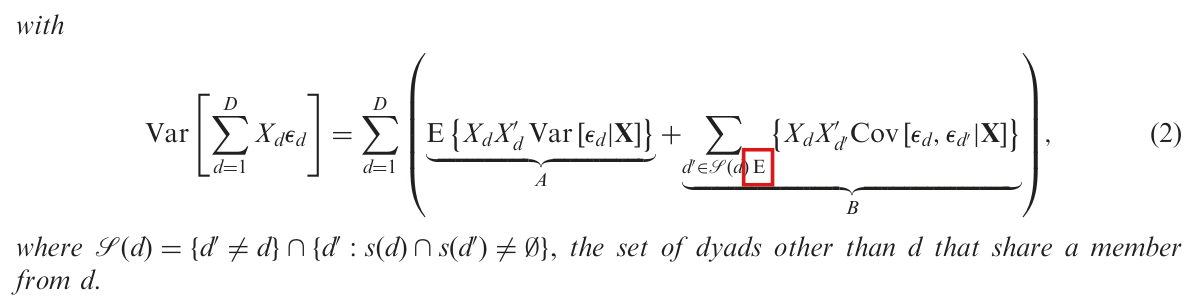
p. 571 (PDF p. 8). The outline marks “lmer package”.

The reference list has two misprints, “BujaAndreas” for “Buja, Andreas” and “ecometrics” for “econometrics”; three other printed forms await a check against the cited works.

References, pp. 576–577 (PDF pp. 13–14): entries Beck et al. (2006), Buja et al. (2014), Hubbard et al. (2010) and White (1984)

As printed

P. 576: Beck, Nathanial, Kristian Skrede Gleditsch, and Kyle Beardsley. 2006. Space is more than geography: Using spatial ecometrics in the study of political economy. […] BujaAndreas, Richard Berk, Lawrence Brown, Edward George, Emil Pitkin, Mikhail Traskin, Linda Zhao, and Kai Zhang. 2014.

P. 577: Hubbard, Alan E., Jennifer Ahern, Nancy L. Fliescher, Mark Van Der Laan, […] ———. 1984. Asymptotic theory of econometricians. New York: Academic Press.

The problem

Every other entry separates the first author’s surname and given name by a comma and a space, and the Buja entry runs them together. The word “ecometrics” in the title of Beck et al. stands for “econometrics”. Three further forms are printed as transcribed: the given name “Nathanial”, the surname “Fliescher” and the title “Asymptotic theory of econometricians”. The readings “Nathaniel”, “Fleischer” and “Asymptotic theory for econometricians” are plausible, but they have not been checked against the cited works.

Evidence a check of the printed page

I checked each complete entry on pp. 576–577 against the rest of the list.

What survives

The four cited works remain identifiable, and no result is affected.

Corrected

P. 576: Beck, Nathanial, Kristian Skrede Gleditsch, and Kyle Beardsley. 2006. Space is more than geography: Using spatial econometrics in the study of political economy. […] Buja, Andreas, Richard Berk, Lawrence Brown, Edward George, Emil Pitkin, Mikhail Traskin, Linda Zhao, and Kai Zhang. 2014.

The forms “Nathanial”, “Fliescher” and “Asymptotic theory of econometricians” are to be replaced by “Nathaniel”, “Fleischer” and “Asymptotic theory for econometricians” only after a check against the cited works.

Crop of two reference entries. Red boxes mark the given name Nathanial in the Beck entry, the word ecometrics in its title, and the run-together name BujaAndreas at the start of the next entry.
References, p. 576 (PDF p. 13), entries Beck et al. (2006) and Buja et al. (2014). Marked: “Nathanial”, “ecometrics” and “BujaAndreas”. The second and third are misprints; the first awaits a check.
Crop of the Hubbard reference entry with one line before and after it. A red box marks the surname Fliescher of the third author.
References, p. 577 (PDF p. 14), entry Hubbard et al. (2010). The marked surname “Fliescher” awaits a check against the cited work.
Crop of the last entries under White with one line before and after. A red box marks the title Asymptotic theory of econometricians in the 1984 entry.
References, p. 577 (PDF p. 14), entry White (1984). The marked title “Asymptotic theory of econometricians” awaits a check against the cited work.

In equation (2) the expectation operator of term BB is set inside the summation subscript; it belongs in front of the braces, as in equation (6).

Lemma 1, equation (2), term BB, p. 566 (PDF p. 3)

See also under Formal statements (Lean): P018-T21

As printed
Var⁡[∑d=1DXdϵd]=∑d=1D(E{XdXd′Var⁡[ϵd∣X]}⏟A+∑d′∈S(d) E{XdXd′′Cov⁡[ϵd,ϵd′∣X]}⏟B),(2)\operatorname{Var}\Big[\sum_{d=1}^{D}X_d\epsilon_d\Big]=\sum_{d=1}^{D}\Big(\underbrace{\mathrm{E}\{X_dX_d'\operatorname{Var}[\epsilon_d|\mathbf{X}]\}}_{A}+\underbrace{\sum_{d'\in\mathcal{S}(d)\,\colorbox{#ffe58a}{$\displaystyle \scriptstyle\mathrm{E}$}}\{X_dX_{d'}'\operatorname{Cov}[\epsilon_d,\epsilon_{d'}|\mathbf{X}]\}}_{B}\Big),\qquad(2)
The problem

The letter E is printed on the line of the summation subscript, after d′∈S(d)d'\in\mathcal{S}(d), and no expectation stands before the braces. Term BB is the sum, over the dyads in S(d)\mathcal{S}(d), of the expectations of the cross terms.

Evidence a check of the printed page

The evidence is a check of the page. Equation (6) in Appendix A (p. 573) prints the same term with E in front of the braces.

What survives

Nothing depends on the misprint. The content of equation (2) is a separate matter, treated in P018-E001.

Corrected
Var⁡[∑d=1DXdϵd]=∑d=1D(E{XdXd′Var⁡[ϵd∣X]}⏟A+∑d′∈S(d)E{XdXd′′Cov⁡[ϵd,ϵd′∣X]}⏟B),(2)\operatorname{Var}\Big[\sum_{d=1}^{D}X_d\epsilon_d\Big]=\sum_{d=1}^{D}\Big(\underbrace{\mathrm{E}\{X_dX_d'\operatorname{Var}[\epsilon_d|\mathbf{X}]\}}_{A}+\underbrace{\sum_{d'\in\mathcal{S}(d)}\colorbox{#ffe58a}{$\displaystyle \mathrm{E}$}\{X_dX_{d'}'\operatorname{Cov}[\epsilon_d,\epsilon_{d'}|\mathbf{X}]\}}_{B}\Big),\qquad(2)

This display corrects the position of E only. With the correction of P018-E001, the conditional variance and covariance are also replaced by ϵd2\epsilon_d^2 and ϵdϵd′\epsilon_d\epsilon_{d'}.

Crop of equation (2) with the word 'with' above it and the definition of the set S(d) below it. In the second term, labelled B, the summation sign has the subscript 'd-prime in S(d)' followed by an upright E, which a red box marks. No E stands before the opening brace of the summand.
Equation (2), p. 566 (PDF p. 3). The mark is on the letter E, printed at the end of the summation subscript of term BB.

The variance estimator V^\widehat V of equation (3) need not be positive semi-definite in a finite sample, and a standard error is the square root of a diagonal entry only when that entry is nonnegative.

Sentence after Proposition 1 and equation (3), p. 567 (PDF p. 4)

See also under Formal statements (Lean): P018-T17, P018-T18

As printed

Standard error estimates for β^\widehat\beta are obtained from the square roots of the diagonals of V^\widehat V.

The problem

The sentence carries no restriction, and the paper does not say that a diagonal entry of V^\widehat V can be negative. Let SS be the D×kD \times k matrix whose row dd is edXd′e_d X_d', and let WW be the D×DD \times D matrix such that Wdd′=1W_{dd'} = 1 if the dyads dd and d′d' share a member (including d′=dd' = d) and Wdd′=0W_{dd'} = 0 otherwise. Then equation (3) reads
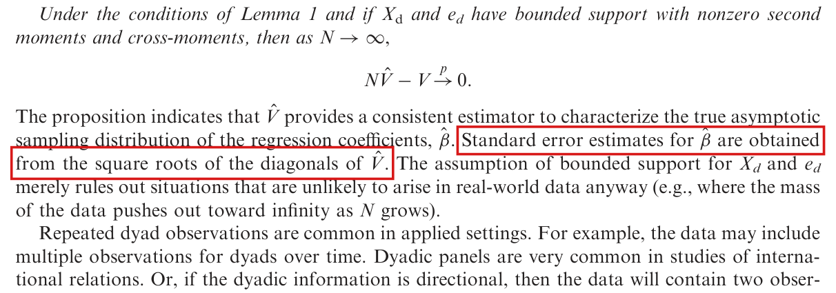
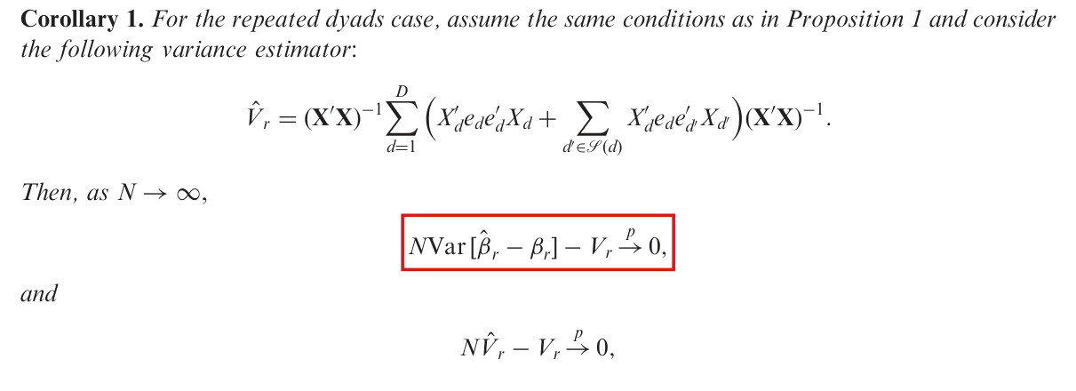
V^=(X′X)−1S′WS (X′X)−1.\widehat V = (\mathbf{X}'\mathbf{X})^{-1} S' W S\, (\mathbf{X}'\mathbf{X})^{-1}.

The matrix WW is not positive semi-definite. For N=4N = 4 its eigenvalues are 55, 11, 11, 11, −1-1, −1-1. A diagonal entry of V^\widehat V can be negative, and the corresponding standard error is then not a real number. In the replication files, the simulation scripts compute sqrt(diag(Vhat)), which returns NaN with a warning in such a draw. A box plot of the saved standard errors then leaves the draw out without notice.

Evidence an exact counterexample

The evidence is an exact counterexample in rational arithmetic. Let N=4N = 4, with one observation per dyad and Xd′=(1,zd)X_d' = (1, z_d), and consider the following data.

An example with N=4N = 4: the regressor zdz_d, the outcome YdY_d and the OLS residual ede_d of each dyad.
Dyadzdz_dYdY_dede_d
{1,2}\{1,2\}11443/53/5
{1,3}\{1,3\}2233−4/5-4/5
{1,4}\{1,4\}33554/54/5
{2,3}\{2,3\}1133−2/5-2/5
{2,4}\{2,4\}2233−4/5-4/5
{3,4}\{3,4\}11443/53/5

By a direct computation, I have

X′X=(6101020),β^=(32/5),X′e=(00),\mathbf{X}'\mathbf{X} = \begin{pmatrix} 6 & 10 \\ 10 & 20 \end{pmatrix}, \qquad \widehat\beta = \begin{pmatrix} 3 \\ 2/5 \end{pmatrix}, \qquad \mathbf{X}'e = \begin{pmatrix} 0 \\ 0 \end{pmatrix},

and the residuals in the last column of the table. Summing XdXd′′eded′X_d X_{d'}' e_d e_{d'} over the pairs of dyads that share a member, as in equation (3), I obtain

S′WS=(−34/25−2−2−98/25),V^=(−17/5021/12521/125−58/625).S'WS = \begin{pmatrix} -34/25 & -2 \\ -2 & -98/25 \end{pmatrix}, \qquad \widehat V = \begin{pmatrix} -17/50 & 21/125 \\ 21/125 & -58/625 \end{pmatrix}.

Both diagonal entries of V^\widehat V are negative. The variance function in the replication files returns the same slope entry, −0.0928-0.0928.

The conditions of Proposition 1 do not exclude these data. Let the characteristics (Ti,Ai)(T_i, A_i) of the units be independent, with TiT_i uniform on {0,1,2,3}\{0, 1, 2, 3\} and AiA_i uniform on {−1,1}\{-1, 1\}. Set zij=∣Ti−Tj∣z_{ij} = |T_i - T_j| and Yij=zij+HTiTj+Ai+AjY_{ij} = z_{ij} + H_{T_i T_j} + A_i + A_j, where the rows and columns of

H=(01−10100−1−10010−110)H = \begin{pmatrix} 0 & 1 & -1 & 0 \\ 1 & 0 & 0 & -1 \\ -1 & 0 & 0 & 1 \\ 0 & -1 & 1 & 0 \end{pmatrix}

are indexed by 0,1,2,30, 1, 2, 3. The data are bounded, with zij∈[0,3]z_{ij} \in [0, 3] and Yij∈[−2,5]Y_{ij} \in [-2, 5]. The matrix E⁡[XdXd′]\operatorname{E}[X_d X_d'] has determinant 15/1615/16, and the covariance matrix of the limiting distribution of N(β^−β)\sqrt{N}(\widehat\beta - \beta) is positive definite, with determinant 67072/5062567072/50625. The event T=(0,1,2,3)T = (0, 1, 2, 3), A=(1,1,1,1)A = (1, 1, 1, 1) has probability 1/40961/4096 and produces the table above. The event T=(3,2,1,0)T = (3, 2, 1, 0), A=(1,1,1,1)A = (1, 1, 1, 1) produces the same table, and the probability of the table is 1/20481/2048.

A second example lies in the simulation design of Section 4. Let N=20N = 20. Let the unit covariates be Xi=iX_i = i for i≤4i \le 4 and Xi=5/2X_i = 5/2 for i≥5i \ge 5, and let αi=0\alpha_i = 0 for all ii. Let νd(1,2)=νd(3,4)=1\nu_{d(1,2)} = \nu_{d(3,4)} = 1 and νd(1,3)=νd(2,4)=−1\nu_{d(1,3)} = \nu_{d(2,4)} = -1, with νd=0\nu_d = 0 for the other dyads. Then X′X\mathbf{X}'\mathbf{X} has determinant 1352413524, and the slope entry of V^\widehat V is

V^22=−3103291528343557147269307≈−0.000712.\widehat V_{22} = -\frac{31032915283}{43557147269307} \approx -0.000712.

The estimator is continuous near this point and the normal density is positive there. A negative slope entry therefore has positive probability in the published design with N=20N = 20. The example does not show how often this occurs.

What survives

This finding does not affect equation (3), Proposition 1 or Proposition 2. Suppose that NV^jjN\widehat V_{jj} converges in probability to a limit V∞,jj>0V_{\infty,jj} > 0. Then

Pr⁡(V^jj<0)≤Pr⁡(∣NV^jj−V∞,jj∣≥V∞,jj)→0,\Pr\bigl(\widehat V_{jj} < 0\bigr) \le \Pr\bigl(|N\widehat V_{jj} - V_{\infty,jj}| \ge V_{\infty,jj}\bigr) \to 0,

and the probability of a negative entry vanishes as NN grows. No value in a published figure or table is shown to be wrong. The replication files do not contain the simulation output, and I cannot determine whether any draw behind Figure 1, or behind Figures 2 and 3 of the Supporting Information, had an undefined standard error.

Corrected

Standard error estimates for β^\widehat\beta are obtained from the square roots of the diagonals of V^\widehat V, for each diagonal entry that is nonnegative. The estimator V^\widehat V need not be positive semi-definite in a finite sample, and a negative diagonal entry has no real-valued standard error. Summaries of simulations should report the number of draws with an undefined standard error and how those draws were treated.

If a value is wanted in every sample, the convention V~jj=max⁡(V^jj,0)\widetilde V_{jj} = \max(\widehat V_{jj}, 0) may be stated separately. This convention changes the estimator in finite samples. Since ∣max⁡(a,0)−max⁡(b,0)∣≤∣a−b∣|\max(a, 0) - \max(b, 0)| \le |a - b| and Vjj≥0V_{jj} \ge 0, it keeps the convergence of NV~jj−VjjN\widetilde V_{jj} - V_{jj} to zero in probability. It does not guarantee coverage or a positive semi-definite matrix.

Crop of ten lines of text and one display from p. 567. The first lines read: Under the conditions of Lemma 1 and if X d and e d have bounded support with nonzero second moments and cross-moments, then as N tends to infinity, N V-hat minus V converges in probability to 0. The paragraph below reads: The proposition indicates that V-hat provides a consistent estimator to characterize the true asymptotic sampling distribution of the regression coefficients, beta-hat. Standard error estimates for beta-hat are obtained from the square roots of the diagonals of V-hat. The assumption of bounded support for X d and e d merely rules out situations that are unlikely to arise in real-world data anyway. The first three lines of the next paragraph, on repeated dyad observations, follow. A red outline in two parts surrounds the sentence that begins Standard error estimates.
Text after Proposition 1, p. 567 (PDF p. 4). The outline marks the sentence that tells how standard errors are obtained from V^\widehat V.

The first conclusion of Corollaries 1 and 2 should describe VrV_r and VwV_w as covariance matrices of limiting distributions, because the variance of the estimator in a finite sample need not exist under the stated conditions.

Corollary 1, first display after “Then, as N→∞N \to \infty”, p. 567 (PDF p. 4); the same display of Corollary 2, p. 575 (PDF p. 12)

See also under Formal statements (Lean): P018-T19, P018-T20

As printed

Corollary 1: … Then, as N→∞N \to \infty,

NVar⁡[β^r−βr]−Vr→p0,\colorbox{#ffe58a}{$\displaystyle N\operatorname{Var}[\widehat\beta_r - \beta_r]$} - V_r \overset{p}{\to} 0,

and

NV^r−Vr→p0,N\widehat V_r - V_r \overset{p}{\to} 0,

Corollary 2: … Then, as N→∞N \to \infty,

NVar⁡[β^w−βw]−Vw→p0,\colorbox{#ffe58a}{$\displaystyle N\operatorname{Var}[\widehat\beta_w - \beta_w]$} - V_w \overset{p}{\to} 0,

and

NV^w−Vw→p0,N\widehat V_w - V_w \overset{p}{\to} 0,
The problem

The first display of each corollary is a statement about the variance of the estimator in a sample of NN units. Under the conditions of the corollaries this variance need not be finite. The estimator contains the inverse of X′X\mathbf{X}'\mathbf{X}, and bounded data with a design of full rank do not bound the moments of that inverse. Convergence in distribution of N(β^−β)\sqrt{N}(\widehat\beta - \beta) and convergence in probability of NV^N\widehat V do not imply that second moments converge. The limiting distribution can have a finite covariance matrix while the estimator has no finite variance at any NN. The proof in Appendix B argues through the mean and the variance of NV^N\widehat V, and these need not be finite either; see P018-E006.

Evidence an exact counterexample

The evidence is an exact counterexample with a derivation. Let the units be independent. For each unit ii, let MiM_i take the value m≥1m \ge 1 with probability 2−m2^{-m}, let CiC_i be uniform on {1,…,m}\{1, \dots, m\} given Mi=mM_i = m, and let AiA_i and BiB_i be independent signs, each equal to ±1\pm 1 with probability 1/21/2. Define δm=1/(m22m2+2)\delta_m = 1/(m^2 2^{m^2 + 2}). For a dyad {i,j}\{i, j\} such that Mi=Mj=mM_i = M_j = m and Ci≠CjC_i \ne C_j, set sij=δms_{ij} = \delta_m and aij=Ai+Aja_{ij} = A_i + A_j. For every other dyad, set sij=1s_{ij} = 1 and aij=0a_{ij} = 0. Each dyad has two observations, so that T(d)=2T(d) = 2, given by

Xij,±=(1,1±sij)′,Yij,±=Bi+Bj±aij.X_{ij,\pm} = (1, 1 \pm s_{ij})', \qquad Y_{ij,\pm} = B_i + B_j \pm a_{ij}.

Note that the regressors lie in [0,2][0, 2] and the outcomes in [−4,4][-4, 4]. The sample residuals are at most 88 in absolute value for all NN and all samples. Every sample design has full rank, and the population matrix E⁡[XX′]\operatorname{E}[X X'] has determinant q=E⁡[s122]≥2/3q = \operatorname{E}[s_{12}^2] \ge 2/3. The population coefficient is βr=0\beta_r = 0, and the OLS slope is

b^=∑i<jsijaij∑i<jsij2.\widehat b = \frac{\sum_{i<j} s_{ij} a_{ij}}{\sum_{i<j} s_{ij}^2}.

Fix N≥3N \ge 3 and m≥N(N−1)m \ge N(N-1), and let EmE_m be the event that Mi=mM_i = m for all ii and that the CiC_i are distinct. On EmE_m every sijs_{ij} equals δm\delta_m, and b^=2Aˉ/δm\widehat b = 2\bar A/\delta_m, where Aˉ\bar A is the mean of the AiA_i. This implies that E⁡[b^2∣Em]=4/(Nδm2)\operatorname{E}[\widehat b^2 \mid E_m] = 4/(N\delta_m^2). Since Pr⁡(Em)≥2−mN−1\Pr(E_m) \ge 2^{-mN-1}, I obtain

E⁡[b^21Em]≥32N m4 22m2−mN≥2m2.\operatorname{E}\bigl[\widehat b^2 \mathbf{1}_{E_m}\bigr] \ge \frac{32}{N}\, m^4\, 2^{2m^2 - mN} \ge 2^{m^2}.

In the last inequality, I used that m≥Nm \ge N. The right side is unbounded in mm. I conclude that E⁡[b^2]=∞\operatorname{E}[\widehat b^2] = \infty for all N≥3N \ge 3, and Var⁡[β^r−βr]\operatorname{Var}[\widehat\beta_r - \beta_r] is not finite. By a parallel computation, the slope entry of V^r\widehat V_r has infinite expectation for all N≥4N \ge 4. The two observations of a dyad may be read as its two directions with unit weights, and the model is then an example for Corollary 2.

In this model N(β^r−βr)\sqrt{N}(\widehat\beta_r - \beta_r) converges in distribution to a normal vector with a finite, positive definite covariance matrix, and NV^rN\widehat V_r converges to that matrix in probability. The second conclusion of each corollary is not contradicted. For the last sentence of the corrected statement, recall that convergence in distribution together with uniform integrability of N∥β^−β∥2N\lVert\widehat\beta - \beta\rVert^2 implies convergence of the first and second moments.

What survives

The second conclusion of each corollary, the estimators V^r\widehat V_r and V^w\widehat V_w, Proposition 2 and every reported number are not affected by this finding. Inference in the paper rests on the limiting distribution and on the convergence of NV^N\widehat V in probability. The statement about the variance of the estimator at finite NN is lost unless a moment condition is added. The example does not satisfy such a condition, and I have not established one for the applications.

Corrected

Apply the repetition and weight regularity conditions in P018-E003, and suppose that the corrected targets in P018-E004 converge to Vr,∞V_{r,\infty} and Vw,∞V_{w,\infty}, respectively.

Corollary 1. For the repeated dyads case, assume the same conditions as in Proposition 1 and consider the following variance estimator:

V^r=(X′X)−1∑d=1D(Xd′eded′Xd+∑d′∈S(d)Xd′eded′′Xd′)(X′X)−1.\widehat V_r = (\mathbf{X}'\mathbf{X})^{-1} \sum_{d=1}^{D} \Bigl( X_d' e_d e_d' X_d + \sum_{d' \in \mathcal{S}(d)} X_d' e_d e_{d'}' X_{d'} \Bigr) (\mathbf{X}'\mathbf{X})^{-1}.

Then, as N→∞N \to \infty, the limiting distribution of N(β^r−βr)\sqrt{N}(\widehat\beta_r - \beta_r) has mean zero and covariance matrix Vr,∞V_{r,\infty}, and

NV^r−Vr→p0.N\widehat V_r - V_r \overset{p}{\to} 0.

If, in addition, N∥β^r−βr∥2N\lVert\widehat\beta_r - \beta_r\rVert^2 is uniformly integrable, then NVar⁡[β^r−βr]−Vr→0N\operatorname{Var}[\widehat\beta_r - \beta_r] - V_r \to 0.

Corollary 2. For the weighted dyads case, assume the same conditions as in Proposition 1 and consider the following variance estimator:

V^w=(X′WX)−1∑d=1D(XdXd′wd2ed2+∑d′∈S(d)XdXd′′wdwd′eded′)(X′WX)−1.\widehat V_w = (\mathbf{X}'\mathbf{W}\mathbf{X})^{-1} \sum_{d=1}^{D} \Bigl( X_d X_d' w_d^2 e_d^2 + \sum_{d' \in \mathcal{S}(d)} X_d X_{d'}' w_d w_{d'} e_d e_{d'} \Bigr) (\mathbf{X}'\mathbf{W}\mathbf{X})^{-1}.

Then, as N→∞N \to \infty, the limiting distribution of N(β^w−βw)\sqrt{N}(\widehat\beta_w - \beta_w) has mean zero and covariance matrix Vw,∞V_{w,\infty}, and

NV^w−Vw→p0.N\widehat V_w - V_w \overset{p}{\to} 0.

If, in addition, N∥β^w−βw∥2N\lVert\widehat\beta_w - \beta_w\rVert^2 is uniformly integrable, then NVar⁡[β^w−βw]−Vw→0N\operatorname{Var}[\widehat\beta_w - \beta_w] - V_w \to 0.

Here VrV_r and VwV_w are the matrices given in P018-E004.

Crop of Corollary 1. The statement reads: For the repeated dyads case, assume the same conditions as in Proposition 1 and consider the following variance estimator, followed by a display that defines V-hat r as a sandwich with a sum over dyads d and over the dyads d-prime in S of d. Then, as N tends to infinity, N Var of beta-hat r minus beta r, minus V r, converges in probability to 0, and N V-hat r minus V r converges in probability to 0. A red outline surrounds the first of the two displays, N Var of beta-hat r minus beta r, minus V r.
Corollary 1, p. 567 (PDF p. 4). The outline marks the first conclusion, which concerns the variance of β^r\widehat\beta_r in a finite sample.
Crop of Corollary 2. The statement reads: For the weighted dyads case, assume the same conditions as in Proposition 1 and consider the following variance estimator, followed by display (7), which defines V-hat w as a weighted sandwich. Then, as N tends to infinity, N Var of beta-hat w minus beta w, minus V w, converges in probability to 0, and N V-hat w minus V w converges in probability to 0. A red outline surrounds the first of the two displays, N Var of beta-hat w minus beta w, minus V w.
Corollary 2, Appendix D, p. 575 (PDF p. 12). The outline marks the first conclusion, which has the same form as in Corollary 1.

With NN fixed and T(d)T(d) growing, serial correlation of fixed order or strong mixing over time can support consistency of β^r\widehat\beta_r, but such assumptions do not in general make the variance estimator V^r\widehat V_r consistent at the scale needed for inference, and Hansen (2007) and Stock and Watson (2008) do not show that they do.

First paragraph after the display that defines VrV_r, fourth and last sentences, p. 568 (PDF p. 5)

As printed

“First, our analysis of the repeated observations case takes the T(d)T(d) values to be fixed and finite and demonstrates consistency as NN grows. […] Under fixed NN and growing T(d)T(d) further assumptions would be required for consistency, such as serial correlation of fixed order or, more generally, strong mixing over time. […] With fixed NN and growing T(d)T(d), however, additional assumptions are needed for consistency (Hansen 2007; Stock and Watson 2008).”

The problem

The paragraph follows Corollary 1, which states that NV^r−VrN\widehat V_r-V_r converges to zero in probability as N→∞N\to\infty with the T(d)T(d) fixed and finite. It introduces no other estimator. In this context I read the two marked sentences as saying that serial correlation of fixed order or strong mixing over time would make V^r\widehat V_r consistent at the scale needed for inference when NN is fixed and T(d)T(d) grows. This is not so. Under suitable conditions, such assumptions support consistency of β^r\widehat\beta_r. Corollary 1 multiplies the variance of β^r\widehat\beta_r and its estimator by NN. In the balanced example below, where T(d)=TT(d)=T, the relevant estimator is TV^rT\widehat V_r, and the named assumptions do not make it consistent. In the example below the errors are independent over time, so that both named assumptions hold. There the ratio of V^r\widehat V_r to the variance of β^r\widehat\beta_r has mean 1/61/6 for every number of periods, and its limit is random.

The two cited papers do not support this reading. Hansen (2007) shows that, for a fixed number of units and a growing number of periods, the clustered covariance estimator is not consistent under strong mixing. It converges in distribution to a random limit; under further homogeneity conditions, inference uses scaled tt and FF reference distributions. Stock and Watson (2008) treat that case with a different estimator, which is adjusted for bias. They note that the clustered covariance estimator averages only across units. Both papers concern panel data, and neither establishes a result for dyadic clustering, where the clusters overlap. Read literally, the two sentences say only that further assumptions are needed, which is true. The paragraph does not specify whether consistency refers to β^r\widehat\beta_r, V^r\widehat V_r, or a different variance estimator.

Evidence an exact counterexample

The evidence is a check of the two cited papers and an exact counterexample. Hansen (2007) studies the clustered covariance estimator W^\widehat W, which contains the products of scores for all pairs of periods within a unit. His Theorem 4 assumes strong mixing, moment conditions, exogeneity and independence across units, and it gives a limit in distribution for W^\widehat W as T→∞T\to\infty with nn fixed. Remark 3.7 (p. 607) reads: “Theorem 4 verifies that W^\widehat W is not consistent but does have a limiting distribution as T→∞T\to\infty with nn fixed.” Corollary 4.1 assumes in addition that the matrices QiQ_i and WiW_i of his notation are the same for all units. Under the null hypothesis, it gives the limit n/(n−1) tn−1\sqrt{n/(n-1)}\,t_{n-1} for the tt-statistic and the limit {nq/(n−q)}Fq,n−q\{nq/(n-q)\}F_{q,n-q} for the Wald statistic with q<nq<n restrictions. Stock and Watson (2008) show that the usual heteroskedasticity-robust estimator can be inconsistent in a regression with fixed effects when T>2T>2 is fixed and nn grows. Their bias-adjusted estimator, equation (6), is consistent under their Assumptions 1–5 when nn or TT grows, “which includes the cases of nn fixed or TT fixed” (equation (7), p. 157). Remark 10 (p. 159) says that the clustered covariance estimator “averages only across entities”. Remark 11 discusses inference with nn fixed and TT growing, and Remark 12 extends the bias-adjusted estimator to serial correlation of finite order. I read Hansen (2007) in a typeset copy that carries the page numbers of the journal, and Stock and Watson (2008) in the published version.

For the counterexample, let N=4N=4 and observe each of the six dyads in the periods t=1,…,Tt=1,\dots,T. The regressor is the constant 11, and Yij,t=ai,t+aj,tY_{ij,t}=a_{i,t}+a_{j,t}, where the ai,ta_{i,t} are independent and equal to 11 or −1-1 with probability 1/21/2 each. Then βr=0\beta_r=0, the data are bounded, and dyads that share no unit are independent. The errors are independent over time, so that their serial correlation has order zero and they are strongly mixing. Let Ai=∑tai,tA_i=\sum_ta_{i,t}, Aˉ=(A1+A2+A3+A4)/4\bar A=(A_1+A_2+A_3+A_4)/4 and Bi=Ai−AˉB_i=A_i-\bar A. Each unit belongs to three dyads, and I have

β^r=A1+A2+A3+A42T,Var⁡[β^r]=1T.\widehat\beta_r=\frac{A_1+A_2+A_3+A_4}{2T},\qquad\operatorname{Var}[\widehat\beta_r]=\frac{1}{T}.

Then β^r\widehat\beta_r is consistent as T→∞T\to\infty. The fitted residuals of the dyad {i,j}\{i,j\} sum over tt to Bi+BjB_i+B_j. Substituting these sums into the estimator of Corollary 1, I obtain

V^r=118T2∑i=14Bi2,RT=V^rVar⁡[β^r]=TV^r=118T∑i=14Bi2.\widehat V_r=\frac{1}{18T^2}\sum_{i=1}^{4}B_i^2,\qquad R_T=\frac{\widehat V_r}{\operatorname{Var}[\widehat\beta_r]}=T\widehat V_r=\frac{1}{18T}\sum_{i=1}^{4}B_i^2.

Since E[∑iBi2]=3T\mathrm{E}[\sum_iB_i^2]=3T, I have E[RT]=1/6\mathrm{E}[R_T]=1/6 for every TT. By a direct computation, I find that Var⁡[RT]=(4T−3)/(216T)\operatorname{Var}[R_T]=(4T-3)/(216T). Since RT≥0R_T\ge0, Markov’s inequality implies that Pr⁡(RT≤1/2)≥2/3\Pr(R_T\le1/2)\ge2/3 for every TT, and RTR_T does not converge to 11 in probability. As T→∞T\to\infty, the ratio RTR_T converges in distribution to χ32/18\chi^2_3/18. Exact enumeration for T=1,2,3,4,8T=1,2,3,4,8 agrees with these values. The same computation applies to the slope in a regression with dyad fixed effects, for even TT and the regressor xt=(−1)tx_t=(-1)^t. In the example, V^r−Var⁡[β^r]\widehat V_r-\operatorname{Var}[\widehat\beta_r] converges to zero in probability, because both terms do, although their ratio does not converge to one.

A second example supports the literal statement that further assumptions are needed. Suppose that each ai,ta_{i,t} is replaced by a sign aia_i that is drawn once and kept in every period. Then β^r=(a1+a2+a3+a4)/2\widehat\beta_r=(a_1+a_2+a_3+a_4)/2 for every TT, and β^r\widehat\beta_r is not consistent.

What survives

No result of the paper depends on the two sentences. Corollary 1 concerns N→∞N\to\infty with the T(d)T(d) fixed and finite, and this finding does not bear on it. No subsequent theorem, simulation or application invokes a fixed-NN, growing-T(d)T(d) consistency result. Section 4 varies NN with one or two observations per dyad, and Section 5 invokes no result for fixed NN and growing T(d)T(d). What changes is the suggestion that assumptions on the dependence over time would make V^r\widehat V_r consistent at the scale needed for inference when NN is fixed. I have not shown that no added assumption can do so, and neither cited paper establishes a result for dyadic clustering.

Corrected

The fourth sentence becomes: “Under fixed NN and growing T(d)T(d), the consistency result above does not apply. Assumptions such as serial correlation of fixed order or, more generally, strong mixing over time can support consistency of β^r\widehat\beta_r under suitable conditions, but they do not in general make V^r\widehat V_r consistent at the scale needed for inference.”

The last sentence becomes: “With fixed NN and growing T(d)T(d), however, inference with a fixed number of units, or a consistent alternative variance estimator, requires a separate analysis. Hansen (2007) and Stock and Watson (2008) give such analyses for panel data, and their results do not establish the corresponding statements for dyadic clustering.”

Crop of fifteen lines of text from p. 568: the paragraph that begins 'Some remarks are in order when it comes to the repeated observations case' and the first two lines of the next paragraph. A red outline in two parts surrounds 'such as serial correlation of fixed order or, more generally, strong mixing over time' in the sentence 'Under fixed N and growing T(d) further assumptions would be required for consistency, such as serial correlation of fixed order or, more generally, strong mixing over time.' A second red outline surrounds '(Hansen 2007; Stock and Watson 2008)' at the end of the sentence 'With fixed N and growing T(d), however, additional assumptions are needed for consistency (Hansen 2007; Stock and Watson 2008).'
First paragraph after the display that defines VrV_r, p. 568 (PDF p. 5). The marks are on the assumptions named in the fourth sentence and on the two citations that end the paragraph.

The dyad-level shock in the list of independent draws is νd(i,j)t\nu_{d(i,j)t}, not ud(i,j)tu_{d(i,j)t}.

Section 4, sentence after equation (4), p. 569 (PDF p. 6)

See also under Formal statements (Lean): P018-T22

As printed

… XiX_i, XjX_j, αi\alpha_i, αj\alpha_j, and ud(i,j)t\colorbox{#ffe58a}{$u_{d(i,j)t}$} are independent draws from standard normal distributions, and the compound error, ϵd(i,j)t=αi+αj+νd(i,j)t\epsilon_{d(i,j)t} = \alpha_i + \alpha_j + \nu_{d(i,j)t}, is unobserved.

The problem

Equation (4) and the compound error in the same sentence write the shock as νd(i,j)t\nu_{d(i,j)t}. No ud(i,j)tu_{d(i,j)t} is defined.

Evidence a check of the printed page

I checked the printed page.

What survives

The simulation design and all results are unchanged.

Corrected

… XiX_i, XjX_j, αi\alpha_i, αj\alpha_j, and νd(i,j)t\colorbox{#ffe58a}{$\nu_{d(i,j)t}$} are independent draws from standard normal distributions, and the compound error, ϵd(i,j)t=αi+αj+νd(i,j)t\epsilon_{d(i,j)t} = \alpha_i + \alpha_j + \nu_{d(i,j)t}, is unobserved.

Crop of equation (4) and six lines of text. Equation (4) reads: Y d(i,j)t equals beta 0 plus beta 1 times the absolute value of X i minus X j, plus alpha i plus alpha j plus nu d(i,j)t, where an underbrace labels the last three terms epsilon d(i,j)t. The text reads: where Y d(i,j)t is the tth observed outcome for the dyad that includes units i and j, X i, X j, alpha i, alpha j, and u d(i,j)t are independent draws from standard normal distributions, and the compound error, epsilon d(i,j)t equals alpha i plus alpha j plus nu d(i,j)t, is unobserved. A red outline surrounds the symbol u d(i,j)t at the start of the second line of text.
Section 4, p. 569 (PDF p. 6): equation (4) and the sentence after it. The outline marks ud(i,j)tu_{d(i,j)t} in the list of independent draws.

The illustration of the misspecified simulation design is Figure 4 of the Supporting Information, and not in the Appendix.

Section 4, p. 570 (PDF p. 7), paragraph after Figure 1

As printed

The degree of misspecification in this case is not extreme (as illustrated in the Appendix) and resembles the kind of approximations that are common in applied work (Buja et al. 2014).

The problem

Appendices A–E (pp. 573–576) contain the proofs and the extensions to weighted observations and generalized linear models. They contain no illustration of the misspecified design. The scatter plot with its linear approximation is Figure 4 on p. 3 of the Supporting Information, and p. 4 there discusses it. On p. 565 the article distinguishes its appendix from this supplement, which it calls the supplementary information.

Evidence a check of the printed page

I checked the pages: p. 570, Appendices A–E, and pp. 3–4 of the Supporting Information, where Figure 4 has the caption “Illustrative scatter plot and linear approximation for the misspecification case”.

What survives

Only the cross-reference changes. No result depends on it.

Corrected

The degree of misspecification in this case is not extreme (as illustrated in Figure 4 of the supplementary information) and resembles the kind of approximations that are common in applied work (Buja et al. 2014).

Crop of five lines of the paragraph after Figure 1. Red boxes mark the words (as illustrated in the, at the end of one line, and Appendix), at the start of the next line.
P. 570 (PDF p. 7), paragraph after Figure 1. The marked parenthesis points to the Appendix, while the illustration is Figure 4 of the Supporting Information.

In Appendix E the second score in B\mathbf B takes the same data argument DD as the first, and the logistic index is the scalar Xd′β^X_d'\hat\beta.

Appendix E, p. 576 (PDF p. 13): display defining A\mathbf A and B\mathbf B, and the definition of pdp_d

See also under Formal statements (Lean): P018-T23

As printed

Given an estimating equation, ψ(D;θ)\psi(D;\theta), on data DD, and with parameters θ\theta and parameter estimates θ^\hat\theta, the sandwich approximation for the variance is A−1B{A−1}′\mathbf A^{-1}\mathbf B\{\mathbf A^{-1}\}', where

A=E[−∂∂θ′ψ(D;θ^)] and  B=E ψ(D;θ^)ψ(Di;θ^)′.\mathbf A=\mathrm E\Big[-\frac{\partial}{\partial\theta'}\psi(D;\hat\theta)\Big]\ \text{and}\ \ \mathbf B=\mathrm E\,\psi(D;\hat\theta)\psi(D_{\colorbox{#ffe58a}{$\displaystyle i$}};\hat\theta)'.

[…] where pd=expit⁡(Xdβ^)p_d=\operatorname{expit}(\colorbox{#ffe58a}{$\mathbf X_d\hat\beta$}), the predicted probability for dyad dd.

The problem

No DiD_i is defined. The paragraph defines the data DD, the parameter and the estimating function ψ(D;θ)\psi(D;\theta), and B\mathbf B is the second moment of the score that defines A\mathbf A. In the logistic index, XdX_d and β^\hat\beta are both column vectors of length kk, so their product is not defined for k>1k>1. The article writes the regression as Yd=Xd′β+ϵdY_d=X_d'\beta+\epsilon_d on p. 566, and the scalar Xd′β^X_d'\hat\beta is meant. The symbol is also set in bold here, while the regressor of a dyad is XdX_d elsewhere.

Evidence a derivation

I checked the page and the dimensions. Let s=ψ(D;θ^)s=\psi(D;\hat\theta), a vector with the dimension of θ\theta. Then E[ss′]\mathrm E[ss'] is a square matrix of the dimension of A\mathbf A, as the product A−1B{A−1}′\mathbf A^{-1}\mathbf B\{\mathbf A^{-1}\}' requires. For k>1k>1 the product of two k×1k\times1 vectors is not defined, and Xd′β^X_d'\hat\beta is the scalar index of the logistic model.

What survives

The intended score moment and the predicted probability are unchanged. The paragraph says that DD denotes the data here, and this second use of the symbol, beside DD for the number of dyads, is not an error. The cross term of the estimator V^l\hat V_l that follows is corrected in P018-E005.

Corrected

Given an estimating equation, ψ(D;θ)\psi(D;\theta), on data DD, and with parameters θ\theta and parameter estimates θ^\hat\theta, the sandwich approximation for the variance is A−1B{A−1}′\mathbf A^{-1}\mathbf B\{\mathbf A^{-1}\}', where

A=E[−∂∂θ′ψ(D;θ^)] and  B=E[ψ(D;θ^)ψ(D;θ^)′].\mathbf A=\mathrm E\Big[-\frac{\partial}{\partial\theta'}\psi(D;\hat\theta)\Big]\ \text{and}\ \ \mathbf B=\mathrm E\big[\psi(D;\hat\theta)\psi(\colorbox{#ffe58a}{$\displaystyle D$};\hat\theta)'\big].

[…] where pd=expit⁡(Xd′β^)p_d=\operatorname{expit}(\colorbox{#ffe58a}{$X_d'\hat\beta$}), the predicted probability for dyad dd.

Crop of the first paragraph of Appendix E, the display defining the matrices A and B, the logistic estimating equation, and the line that defines p d. One red box marks the argument D with subscript i in the second factor of B. A second red box marks expit of X d beta hat, printed with a bold X and no prime.
Appendix E, p. 576 (PDF p. 13). Marked: the argument DiD_i of the second score in B\mathbf B, and the logistic index printed without a transpose.

Clarity notes

Imprecise or ambiguous wording whose intended meaning is correct; not an error.

“Sizes that are far too small” means tests that reject too often and confidence intervals that are too narrow, and “t>1.64t>1.64” means that the absolute value of the tt-ratio is compared with 1.64.

Section 1, first paragraph, p. 565 (PDF p. 2); Section 5, second paragraph, p. 571 (PDF p. 8)

As printed

p. 565: “Failure to account for dyadic clustering may result in significance tests or confidence intervals with sizes that are far too small relative to the true distribution of the parameters of interest.”

p. 571: “But when one takes into account dyadic clustering, the coefficient for international organizations would fail to pass a conventional significance test (e.g., t>1.64t>1.64).”

Intended meaning

The sentence on p. 565 says that the uncertainty of the estimates is understated when dyadic clustering is ignored. Standard errors that are too small make a test reject a true null hypothesis too often, so that its size is too large, and they make confidence intervals too narrow. The distribution meant is the sampling distribution of the coefficient estimates, and the Conclusion (p. 572) describes the same failure as “seriously anti-conservative”. On p. 571 the coefficient is negative, and the comparison intended is between the absolute value of the tt-ratio and 1.64. Table 1 reports −0.011-0.011 and 0.0080.008 for international organizations, and their ratio is −11/8-11/8. Allowing for the rounding of both entries, the absolute ratio lies between 21/1721/17 and 23/1523/15, below 1.64, and the conclusion about this coefficient stands.

Corrected

p. 565: “Failure to account for dyadic clustering may result in significance tests that overreject and confidence intervals that are too narrow relative to the sampling distribution of the coefficient estimates.”

p. 571: “… would fail to pass a conventional significance test (e.g., ∣t∣>1.64|t|>1.64 for an approximately 10% two-sided normal test).”

Crop of seven lines from the first paragraphs of page 565. Red boxes mark the phrases 'sizes that are far too small' and 'true distribution of the parameters of interest.' in the sentence 'Failure to account for dyadic clustering may result in significance tests or confidence intervals with sizes that are far too small relative to the true distribution of the parameters of interest.'
Section 1, first paragraph, p. 565 (PDF p. 2). The marks are on “sizes that are far too small” and on “true distribution of the parameters of interest”.
Crop of six lines from Section 5 on page 571. A red box marks 't > 1.64' in the sentence 'But when one takes into account dyadic clustering, the coefficient for international organizations would fail to pass a conventional significance test (e.g., t > 1.64).'
Section 5, second paragraph, p. 571 (PDF p. 8). The mark is on “t>1.64t>1.64”.

In Appendix A, “the finite support of XdX_d and ede_d” means the bounded support assumed in Proposition 1, and the first XdX_d of the proposition has an upright subscript.

Proposition 1, p. 567 (PDF p. 4); Appendix A, proof of Lemma 1, p. 573 (PDF p. 10)

As printed

p. 567: “Under the conditions of Lemma 1 and if XdX_{\colorbox{#ffe58a}{$\mathrm{d}$}} and ede_d have bounded support with nonzero second moments and cross-moments, then as N→∞N\to\infty”

p. 573: “By continuity of the inverse, the finite support of XdX_d and ede_d, X\mathbf{X} full rank, and the fact that the sum of dependent terms in this sum is O(D3/2)O(D^{3/2}) (Lehmann 1999, Equation (2.8.4)), we have that”

Intended meaning

Proposition 1 assumes that the regressors XdX_d and the fitted residuals ed=Yd−Xd′β^e_d=Y_d-X_d'\hat\beta have bounded support. A fitted residual is a random variable, and a condition on its support is meaningful. Bounded XdX_d and YdY_d bound the population residual ϵd\epsilon_d, but they do not by themselves bound ede_d uniformly in NN. The corrected proof in P018-E006 establishes the conclusion of Proposition 1 without this condition. Appendix A recalls this hypothesis, and “finite support” there refers to support bounded in a finite interval, as on p. 566, and not to a distribution with finitely many values. The upright d\mathrm{d} is the index dd. Nothing depends on either point.

Corrected

p. 567: “Under the conditions of Lemma 1 and if XdX_{\colorbox{#ffe58a}{$d$}} and ede_d have bounded support with nonzero second moments and cross-moments, then as N→∞N\to\infty”

p. 573: “By continuity of the inverse, the bounded support of XdX_d and ede_d, X\mathbf{X} full rank, …”

Crop of Proposition 1 with equation (3), the sentence 'Under the conditions of Lemma 1 and if X_d and e_d have bounded support with nonzero second moments and cross-moments, then as N goes to infinity', and the display 'N V-hat minus V converges in probability to 0'. A red box marks the first X_d, whose subscript d is upright while the other subscripts are italic.
Proposition 1, p. 567 (PDF p. 4). The mark is on the first XdX_d of the sentence, whose subscript is upright.
Crop of the start of the proof of Lemma 1: a display for root-N times beta-hat minus beta, the sentence 'By continuity of the inverse, the finite support of X_d and e_d, X full rank, and the fact that the sum of dependent terms in this sum is O(D to the power 3/2) (Lehmann 1999, Equation (2.8.4)), we have that', and a second display. A red box marks 'finite support'.
Appendix A, proof of Lemma 1, p. 573 (PDF p. 10). The mark is on “finite support”.

Formal statements (Lean)

Formal results: 23 whole; 2 restricted; 3 refuted; 0 omitted.

Coverage concerns the identified claim under its stated assumptions. A checked proof establishes the formal statement; correspondence to the published text was reviewed by AI. Repository access is currently required to open the source links.

Each result links to its current formal statement and proof. “Whole” covers the identified claim under its assumptions; “restricted” covers the stated narrower scope; “refuted” gives a counterexample to the identified assertion; “omitted” has no current theorem. Any named published theorem used as a premise remains an assumption. Browse the formal results for this work.

Lemma 1, equation (2), with the second and third lines of equation (6) (Appendix A), the population Σ\Sigma of Appendix B and the conditional ‘meat’ of VrV_r and VwV_w: an exact bounded, full-rank dyadic model in which the printed right-hand side is the zero matrix for every NN and the true variance is positive definite at leading order (the validator's construction; not in the paper)

p. 566 (PDF p. 3), eq. (2); p. 573 (PDF p. 10), eq. (6) and Σ\Sigma; p. 568 (PDF p. 5), VrV_r; p. 576 (PDF p. 13), VwV_w

p. 566 (PDF p. 3), equation (2); p. 573 (PDF p. 10), equation (6) and Sigma; pp. 568, 576, V_r and V_w. For iid uniform units, X=(1,2+Z_i+Z_j) and Y=(Z_i+Z_j)^2 satisfy the bounded dyadic projection assumptions and almost-sure sample rank. The conditional mean is quadratic and not affine. All printed conditional covariance meats, including the singleton repeated and unit-weight extensions, are zero. The centred scores have the displayed H, overlapping Gamma, exact nonzero finite variance and positive leading limit. The true target tends to 4 Q^{-1} Gamma Q^{-1}=V_*, the scaled estimator has that Gaussian limit, and the sandwich converges in probability to V_*. The usual measure-theoretic conditions are assumed.

Historical component credits
  • Proved AronowAudit.P018.Wave1.nonlinear_counterexample_proof Historical support retained; baseline fidelity: ok; manifest: used; used in Solution; The row supplies an exact counterexample to the printed covariance equality and the stated CLT and consistency limits; the repeated and unit-weight formulations of T1(f) are not exported by any row read here.
  • Proved AronowAudit.P018.nonlinear_matrix_certificate Historical support retained; baseline fidelity: ok; manifest: used; used in Solution; Fidelity sweep: ok
  • Proved AronowAudit.P018.nonlinear_bounds Historical support retained; baseline fidelity: ok; manifest: used; used in Solution; Fidelity sweep: ok
  • Proved AronowAudit.P018.nonlinear_matrices_positive Historical support retained; baseline fidelity: ok; manifest: used; used in Solution; Supporting fact already subsumed by a retained main row; not called separately in the Solution.
  • Proved AronowAudit.P018.nonlinear_model_assumptions Historical support retained; baseline fidelity: ok; manifest: used; used in Solution; Supporting fact already subsumed by a retained main row; not called separately in the Solution.
  • Proved AronowAudit.P018.nonlinear_population_projection Historical support retained; baseline fidelity: ok; manifest: used; used in Solution; Fidelity sweep: ok
  • Proved AronowAudit.P018.uniform_pair_monomial Historical support retained; baseline fidelity: ok; manifest: used; used in Solution; Supporting fact already subsumed by a retained main row; not called separately in the Solution.
  • Proved AronowAudit.P018.uniform_pair_monomial_integrable Historical support retained; baseline fidelity: ok; manifest: used; used in Solution; Supporting fact already subsumed by a retained main row; not called separately in the Solution.
  • Proved AronowAudit.P018.uniform_polynomial_integral Historical support retained; baseline fidelity: ok; manifest: used; used in Solution; Supporting fact already subsumed by a retained main row; not called separately in the Solution.
  • Proved AronowAudit.P018.uniform_unit_moment Historical support retained; baseline fidelity: ok; manifest: used; used in Solution; Supporting fact already subsumed by a retained main row; not called separately in the Solution.
  • Proved AronowAudit.P018.uniform_unit_moments Historical support retained; baseline fidelity: ok; manifest: not used; not used in Solution; Supporting fact already subsumed by a retained main row; not called separately in the Solution.
  • Proved AronowAudit.P018.uniform_unit_power_L2 Historical support retained; baseline fidelity: ok; manifest: used; used in Solution; Supporting fact already subsumed by a retained main row; not called separately in the Solution.

Lemma 1, equation (2), and equation (6) of Appendix A, corrected: the variance of the score sum in unconditional score moments, with the term that the printed conditional form omits

p. 566 (PDF p. 3), eq. (2); p. 573 (PDF p. 10), eq. (6) and the Σ\Sigma of Appendix B

p. 566 (PDF p. 3), equation (2); p. 573 (PDF p. 10), equation (6) and Appendix B; p. 568 and p. 576, repeated and weighted covariance targets. Under the usual measure-theoretic conditions, the symmetric iid single-record model has centered scores, zero disjoint raw moments, the corrected sparse second-moment meat, the full law of total covariance and its omitted positive semidefinite term, the disjoint conditional remainder, the overlap representation of Gamma, and the exact finite-N and limiting sandwiches. Projection orthogonality alone need not remove the omitted term. For bounded finite repeated records and fixed real weights with nonsingular population Gram, the total score is centered; its covariance equals the full raw double sum and the sparse unconditional covariance sum. The sparse raw sum is valid exactly when the sparse block-mean products cancel, in particular if every block is centered. Global centering alone is insufficient. The repeated and weighted targets use N/L^2 and N/D^2, respectively. No fitted-residual consistency is asserted here.

Historical component credits
  • Proved AronowAudit.P018.Wave1.variance_correction_proof Historical support retained; baseline fidelity: ok; manifest: used; used in Solution; Standing matches S9 and the intercept requirement in S2; boundedness and measurability make the covariance and conditional-expectation integrals genuine, and no conditional exogeneity is assumed.
  • Proved AronowAudit.P018.variance_sparse_identity Historical support retained; baseline fidelity: ok; manifest: used; used in Solution; Generic sparse helper is not called separately; the retained kernel-level sparse identity is already exported.
  • Proved AronowAudit.P018.Wave1.conditional_moment_correction_proof Historical support retained; baseline fidelity: ok; manifest: used; used in Solution; The comparison is to corrected T2(ii) and the sufficient condition in (iii); using uncentered conditional products is the requested correction itself, not a mismatch with that target.

Appendix B (proof of Proposition 1): exact bounded, full-rank model in which the printed mean condition, the printed limit E[Σ^]→Σ\mathrm{E}[\hat\Sigma]\to\Sigma and the printed dependence count for products of fitted residuals fail, while the conclusion of Proposition 1 holds; with the examples showing that convergence in probability of the inverse Gram matrix gives no moment control (the validators' constructions; not in the paper)

pp. 573–574 (PDF pp. 10–11), Appendix B

pp. 573-574 (PDF pp. 10-11), Appendix B. In the intercept fair-sign model the fit, residual bound, ordered-overlap identity, exact meat, target, means, fourth moments and scaled variance have the displayed formulas. The raw mean error diverges while its normalized version vanishes, and the sandwich remains consistent. Products of fitted residuals on disjoint endpoint unions have the stated positive covariance, while another covariance is negative; these are actual OLS residuals and the disjoint configuration lies outside the six printed cases. The deterministic missing-N and spike examples invalidate the printed moment inferences. The bounded inverse-design example has determinant twice Var(exp(-T))>0, almost-sure rank for every N>=3, inverse convergence in probability and the displayed infinite extended inverse-norm expectation for every N>=3. The usual measure-theoretic conditions are assumed.

Historical component credits
  • Proved AronowAudit.P018.Wave1.appendixB_counterexample_proof Historical support retained; baseline fidelity: ok; manifest: used; used in Solution; Role: witness to the printed proof’s mean step plus the positive consistency result in that witness, not a refutation of Proposition 1. The row expressly excludes the other T3 components. Claim-stage verdict retained.
  • Counterexample proved AronowAudit.P018.missing_N_counterexample Historical support retained; baseline fidelity: ok; manifest: used; used in Solution; Role: a full counterexample to the scalar logical sufficiency implication using the printed unscaled mean condition, not a claim that the deterministic estimator is an OLS sandwich. Claim-stage verdict retained.
  • Proved AronowAudit.P018.sign_mean_counterexample Historical support retained; baseline fidelity: ok; manifest: not used; not used in Solution; Four-unit finite means are redundant with the retained general-N expectation counterexample.
  • Proved AronowAudit.P018.intercept4_fit Historical support retained; baseline fidelity: ok; manifest: not used; not used in Solution; Only the four-unit fit; does not supply the omitted general-N fit clause.
  • Counterexample proved AronowAudit.P018.fitted_products_counterexample Historical support retained; baseline fidelity: ok; manifest: used; used in Solution; {'source': 'adjudication', 'decision': 'rejected', 'what': 'P018/P018_Audit.lean:2236 gives exactly the three N=8 covariance values in the covered finite-witness component of T3(g): 7/16 for fitted products on disjoint unit sets, zero for the corresponding population products, and -1/16 for the other fitted products. The definitions at lines 2227 and 2230 use the actual intercept-only fitted residuals and covariance under the recursive fair-sign average. That average assigns probability 1/256 to each iid sign outcome, so this is a faithful finite probability representation.'}
  • Proved AronowAudit.P018.Wave1.inverse_spike_counterexample_proof Historical support retained; baseline fidelity: ok; manifest: used; used in Solution; Role: the standalone T3(h) probability witness, with no assertion that R_N is itself an inverse Gram matrix. Claim-stage verdict retained.
  • Proved AronowAudit.P018.Wave1.inverse_gram_counterexample_proof Limited support; baseline fidelity: narrower; manifest: used; used in Solution; {'source': 'adjudication+second review', 'adjudicator': "P018/Wave1/Gap/GLP0182B1.lean:443 exports Standing inverseKernel and SampleRank inverseKernel, but SampleRank at P018/P018_Audit.lean:754 only asserts an unspecified eventual threshold for almost-sure sample nonsingularity. T3(i) instead asserts full sample rank almost surely for every N >= 3, and the credited declaration does not state that threshold. It also omits T3(i)'s exact identity det Q = 2 Var(exp(-T)), exporting nonsingularity through Standing instead. The explicit design, inverse probability limit, lower bounds and infinite inverse moments match the target, but do not supply those omitted conclusions.", 'suggested_fix': 'Extend the credited conjunction with almost-sure det(sampleGram) != 0 for every N >= 3, and det(populationGram inverseKernel) = 2 * Var(exp(-T)) > 0 under paretoUnitLaw. Keep the existing inverse-moment conclusions; an existential SampleRank threshold alone does not state the required finite-N rank result.', 'second_review': "P018/Wave1/Gap/GLP0182B1.lean:443 exports only an unspecified eventual rank threshold through SampleRank at P018/P018_Audit.lean:754, rather than T3(i)'s almost-sure full rank for every N>=3. It also omits the target identity det Q=2*Var(exp(-T)), although the explicit design at P018/P018_Audit.lean:2324 and its infinite inverse-moment conclusions match. These are minor elementary additions: the finite-N rank follows from the distinct-coordinate and positive-determinant lemmas at P018/Wave1/Gap/GLP0182B1.lean:201 and P018/Wave1/Gap/GLP0182B1.lean:180, while det Q=Var(Z_1+Z_2)=2*Var(Z_1) is the two-by-two moment expansion under the product law. Export these conclusions explicitly without changing the core inverse-moment witness.", 'severity': 'minor'}

Proposition 1 with a corrected proof (replacement for Appendix B): consistency of NV^N\hat V for the target of equation (1) by a probability-limit argument, with the corrected Chebyshev conditions

p. 567 (PDF p. 4), Proposition 1; pp. 573–574 (PDF pp. 10–11), Appendix B

p. 567 (PDF p. 4), Proposition 1; pp. 573–574 (PDF pp. 10–11), Appendix B. The dyadic sandwich is absolutely consistent for the unconditional target, and the correctly scaled finite-moment Chebyshev conditions are sufficient.

Historical component credits
  • Proved AronowAudit.P018.Wave1.variance_consistency_corrected_proof Historical support retained; baseline fidelity: ok; manifest: used; used in Solution; {'source': 'adjudication', 'decision': 'rejected', 'what': "P018/Wave1/Gap/GLP0182B2.lean:325 assumes only Standing and concludes N times the actual sandwich estimator minus the unconditional score-variance target converges in probability to zero, matching the main assertion of T4. Standing in P018/P018_Audit.lean:725 contains the bounded symmetric iid-unit model, intercept, and population rank supplied by the standing assumptions, with no nondegeneracy or inverse-moment condition. The maximum-entry norm is equivalent to the target's operator norm in fixed dimension, and the zero inverse on singular samples is an allowed completion in the claim."}
  • Proved AronowAudit.P018.members_card Historical support retained; baseline fidelity: ok; manifest: used; used in Solution; Supporting fact already subsumed by a retained main row; not called separately in the Solution.
  • Proved AronowAudit.P018.number_of_dyads Historical support retained; baseline fidelity: ok; manifest: used; used in Solution; Supporting fact already subsumed by a retained main row; not called separately in the Solution.
  • Proved AronowAudit.P018.sandwich_difference Historical support retained; baseline fidelity: ok; manifest: used; used in Solution; Supporting fact already subsumed by a retained main row; not called separately in the Solution.
  • Proved AronowAudit.P018.corrected_chebyshev Historical support retained; baseline fidelity: ok; manifest: used; used in Solution; Role: the finite scalar bound. Finite mean and variance in the target’s “whenever the moments exist” reading are equivalent to the L² condition; no asymptotic sequence conclusion is claimed by this row. Claim-stage verdict retained.
  • Proved AronowAudit.P018.Wave1.dyad_counts_proof Historical support retained; baseline fidelity: ok; manifest: not used; not used in Solution; Supporting fact already subsumed by a retained main row; not called separately in the Solution.
  • Proved AronowAudit.P018.residual_substitution_bound Historical support retained; baseline fidelity: ok; manifest: used; used in Solution; Supporting fact already subsumed by a retained main row; not called separately in the Solution.
  • Proved AronowAudit.P018.normalized_overlap_coefficient Historical support retained; baseline fidelity: ok; manifest: not used; not used in Solution; Supporting fact already subsumed by a retained main row; not called separately in the Solution.
  • Proved AronowAudit.P018.Wave1.population_meat_variance_bounds_proof Historical support retained; baseline fidelity: ok; manifest: not used; not used in Solution; Supporting fact already subsumed by a retained main row; not called separately in the Solution.
  • Proved AronowAudit.P018.normalized_sample_sandwich Historical support retained; baseline fidelity: ok; manifest: not used; not used in Solution; Supporting fact already subsumed by a retained main row; not called separately in the Solution.

Section 4 and Supporting Information: the claim that design (4) with normal data ‘corresponds precisely to the assumptions of’ the fitted two-way normal random effects model. Exact covariance mismatch between design (4) and the model fitted in the replication archive, with an exact consequence for a model-based standard error (the validators' calculations; not in the paper)

pp. 569–570 (PDF pp. 6–7), paragraph beginning ‘In the supplementary information’; Supporting Information p. 2; p. 572 (PDF p. 9), Conclusion; replication scripts 1 (line 86) and 2 (line 78)

pp. 569–570 (PDF pp. 6–7), paragraph beginning ‘In the supplementary information’; Supporting Information p. 2; p. 572 (PDF p. 9), Conclusion; replication scripts 1 (line 86) and 2 (line 78). The three-unit two-role covariance family misses the shared-unit covariance and understates the displayed GLS variance.

Historical component credits
  • Counterexample proved AronowAudit.P018.two_role_counterexample Historical support retained; baseline fidelity: ok; manifest: used; used in Solution; This is a harmless algebraic generalization of the N=3 witness, not proof of the target general-N count or repeated-observation comparison.
  • Counterexample proved AronowAudit.P018.gls_variance_counterexample Historical support retained; baseline fidelity: ok; manifest: used; used in Solution; Fidelity sweep: ok
  • Proved AronowAudit.P018.Wave1.random_intercept_lower_bound_proof Historical support retained; baseline fidelity: ok; manifest: used; used in Solution; {'source': 'adjudication', 'decision': 'rejected', 'what': 'P018/Wave1/Gap/GP0182B1.lean:319 states precisely the conditional variance decomposition and lower bound in T5(f), assuming the centered response is independent of the Gaussian average as that component specifies. Estimator measurability expresses the usual statistical meaning of an estimator, and the two L2 premises are equivalent under translation equivariance because the Gaussian shift is L2. The construction of the centered response is a different component; no cases of the conditional bound credited here are lost.'}

Section 4 and Supporting Information, the correspondence between design (4) and the random-effects benchmark, corrected: the shared-unit random-effects covariance that does match design (4), and the statement that the fitted two-role model is covariance-misspecified

pp. 569–570 (PDF pp. 6–7); Supporting Information p. 2; p. 572 (PDF p. 9)

pp. 569–570 (PDF pp. 6–7); Supporting Information p. 2; p. 572 (PDF p. 9). Shared-unit incidence yields the covariance expansion and role mismatch, and using the correct covariance yields the exact GLS covariance.

Historical component credits
  • Proved AronowAudit.P018.Wave1.benchmark_covariance_correction_proof Historical support retained; baseline fidelity: ok; manifest: used; used in Solution; Only the algebraic component is credited here. Together R124-01–04 establish all formal T6(i)–(iv); τ denotes a variance value, not its square root.
  • Proved AronowAudit.P018.shared_role_expansion Historical support retained; baseline fidelity: ok; manifest: not used; not used in Solution; Its incidence expansion is already included in the retained general-N correction row.
  • Proved AronowAudit.P018.correct_gls_identity Historical support retained; baseline fidelity: ok; manifest: used; used in Solution; The broader symmetric invertible domain is harmless; positive definiteness of C and full column rank of F imply the two determinant premises required for the target specialization.
  • Proved AronowAudit.P018.shared_random_effect_covariance Historical support retained; baseline fidelity: ok; manifest: used; used in Solution; Existence of finite covariance in T6(ii) includes finite coordinate second moments, so the L² premises do not exclude its cases. General Z also includes the specified shared-node incidence matrix.

The claim that the conditions of Lemma 1 and Proposition 1 give valid confidence intervals and tests from the square roots of the diagonal of V^\hat V (p. 565; p. 567 after Proposition 1; p. 571, ‘t>1.64t > 1.64’): exact model satisfying the stated conditions in which a coefficient has zero leading variance and its estimated variance is negative with limiting probability 1−e−1/21 - e^{-1/2} (the validator's construction; not in the paper)

p. 567 (PDF p. 4), Proposition 1 and the two sentences after it; p. 565 (PDF p. 2), ‘while our procedure does’; p. 566 (PDF p. 3), Lemma 1

pp. 565-567 (PDF pp. 2-4), Lemma 1 and Proposition 1. The bounded iid sign-pair model has Q=[[1,1],[1,2]], beta=0, the stated residual and score moments, and rank failure probability 2^(1-N). Its exact target tends to diag(4,0). The specified eight-unit sample has positive probability, the displayed Gram, OLS coefficient, meat and negative slope variance. Jointly (N beta_hat_slope,N^2 V_hat_22) tends to (2AB,4(A^2+B^2-1)) for independent standard normals A,B. The negative variance probability tends to 1-exp(-1/2)>0; on such samples no real square root exists. The pivot completed by zero when V_hat_22<=0 has no standard normal limit. Nevertheless N V_hat tends in probability to diag(4,0) and N V_hat-V_N tends to zero. The usual measure-theoretic conditions are assumed; the ordinary inverse is used on full-rank samples and the matrix inverse supplies the zero completion on singular samples.

Historical component credits
  • Proved AronowAudit.P018.Wave1.TailB_degenerate_inference_counterexample Historical support retained; baseline fidelity: ok; manifest: used; used in Solution; {'source': 'adjudication', 'decision': 'rejected', 'what': 'P018/Wave1/Gap/TailBSignDegeneracy.lean:9 exports the specified sign-pair witness, whose statement in P018/P018_Audit.lean:1860 includes the exact negative-variance probability limit, failure of normal studentization, and absolute variance consistency. The zero completion of the pivot on nonpositive variances does not conceal the failure: negative variances themselves have the claimed positive limiting probability. Singular samples are explicitly admitted by T7(a), with exponentially vanishing probability; the finite certificate and joint second-order limits are separate from the main inference-failure component covered here.'}
  • Counterexample proved AronowAudit.P018.degenerate_numeric_certificate Historical support retained; baseline fidelity: ok; manifest: used; used in Solution; Fidelity sweep: ok

The claim of valid confidence intervals and tests from V^\hat V (pp. 565, 567, 571–572), corrected: a non-degeneracy condition for each tested contrast, with the projection central limit theorem that the paper does not state

p. 567 (PDF p. 4), after Proposition 1; p. 565 (PDF p. 2); p. 573 (PDF p. 10), Appendix A

p. 567 (PDF p. 4), after Proposition 1; p. 565 (PDF p. 2); p. 573 (PDF p. 10), Appendix A. Under the standing bounded symmetric unit-kernel model, the projection CLT (allowing singular limits), target limit, and sandwich consistency hold. Every contrast of positive limiting variance has a standard normal zero-extended pivot, vanishing probability of nonpositive estimated variance, and nominal confidence coverage. The shared-endpoint moment equals the projection covariance. The specified zero-variance slope supplies a failure of normal inference.

Historical component credits
  • Proved AronowAudit.P018.Wave1.inference_corrected_proof Historical support retained; baseline fidelity: ok; manifest: used; used in Solution; {'source': 'adjudication', 'decision': 'rejected', 'what': 'P018/Wave1/Gap/GLP0182B3.lean:188 exports the possibly singular Gaussian CLT, convergence of the unconditional target, consistency of N times the sandwich, and standard normal pivots for every positive-variance contrast, matching the covered parts of T8(i)-(iii). Positivity is already required by the corrected claim and is imposed only on the tested contrast. The theorem also states that nonpositive estimated variance has vanishing probability, so totalizing that pivot to zero and completing singular sample inverses do not exclude any eligible model or contrast.'}
  • Proved AronowAudit.P018.Wave1.score_projection_decomposition_proof Historical support retained; baseline fidelity: ok; manifest: not used; not used in Solution; Projection-decomposition helper; the retained CLT and coverage are supplied directly by the inference and coverage rows.
  • Proved AronowAudit.P018.Wave1.contrast_coverage_corrected_proof Historical support retained; baseline fidelity: ok; manifest: used; used in Solution; {'source': 'adjudication', 'decision': 'rejected', 'what': "P018/Wave1/Gap/GP0182B2b.lean:1712 proves two-sided coverage 1-alpha for every fixed contrast with positive limiting variance and every 0<alpha<1, exactly the coverage component of T8(iii). Its normalQuantile is defined from the genuine standard Gaussian distribution in P018/P018_Audit.lean:2285. Excluding negative estimated variance and admitting zero variance only when the error is zero changes no asymptotic coverage, because T8's positive-variance condition makes the probability of nonpositive estimated variance tend to zero."}

Corollary 2 (weighted observations) under ‘weights finite and fixed’: exact model with positive, uniformly bounded, fixed weights and a perfect unweighted design in which the two conclusions of the corollary cannot both hold for any target (the validator's construction; not in the paper)

p. 575 (PDF p. 12), Appendix D and Corollary 2; pp. 567–568 (PDF pp. 4–5), ‘where the T(d)T(d) values are fixed and finite’ and Corollary 1

p. 575 (PDF p. 12), Appendix D and Corollary 2; pp. 567–568 (PDF pp. 4–5), fixed finite repetitions and Corollary 1. The bounded fair-sign intercept model with fixed weights 2^(-i-j) has the stated geometric sums, linear fit, variance bounded below by 9/16 and tending to 36/35, inconsistent coefficients and divergent scaled variance. Its first-eight-positive event has probability 1/256 and forces the stated sandwich separation, ruling out a common deterministic target. The normalized weighted design vanishes and the first coefficient tends to 3/4. Identical repetitions 2^(i+j) transfer the joint law by label reversal and have no uniform count bound. Duplicating both directions preserves the weighted fit and sandwich. The all-N linear-fit and variance identities include the zero completion when N<2.

Historical component credits
  • Proved AronowAudit.P018.Wave1.concentrated_weights_counterexample_proof Historical support retained; baseline fidelity: ok; manifest: used; used in Solution; This is a witness for the joint failure, not a positive consistency claim. The public key_results sentence precisely matches the variance limit and universal deterministic-target exclusion. Metadata inconsistency: T9 has asymptotic=false although its variance limit and exclusion of joint limiting targets are asymptotic.
  • Proved AronowAudit.P018.Wave1.concentrated_repetitions_counterexample_proof Historical support retained; baseline fidelity: ok; manifest: used; used in Solution; This is the law-transfer component, not a standalone inconsistency theorem; R124-06 supplies the failure to transfer. The lower bound N≥2 removes only samples with no dyads.

Corollaries 1 and 2, corrected hypotheses: uniformly bounded repetitions with common record-index kernels and vanishing mean-score overlap, and weights bounded after common rescaling with a non-degenerate normalized weighted design

pp. 567–568 (PDF pp. 4–5), Corollary 1; p. 575 (PDF p. 12), Appendix D and Corollary 2

pp. 567–568 (PDF pp. 4–5), Corollary 1; p. 575 (PDF p. 12), Appendix D and Corollary 2. Uniformly bounded common record kernels and counts, a positive limiting normalized design, and vanishing scaled overlap products of block means imply repeated sandwich consistency. The stacked normal equations alone need not give overlap control or consistency. A common ordered kernel, at most one record per direction, bounded positive normalized weights, and a positive limiting normalized weighted design imply weighted consistency, permitting empty blocks. Positive common weight rescaling leaves all three weighted quantities unchanged where the ordinary inverses exist. Bounded positive fixed weights and unweighted rank alone are insufficient.

Historical component credits
  • Proved AronowAudit.P018.Wave1.repeated_consistency_with_overlap_mean_control Historical support retained; baseline fidelity: ok; manifest: used; used in Solution; {'source': 'adjudication+second review', 'adjudicator': "P018/Wave1/Gap/DecideC.lean:679 requires hMean, namely convergence to zero of the N/L_N^2-scaled overlap meat of expected block scores, whereas the supplied corrected C1 lists bounded repetitions and a positive limiting normalized design. This is a substantive extra premise: with independent fair signs A_i, common X_t = 1, Y_t = A_i + A_j + 1{t = 1} using zero-based record indices, and a second record only for even-even unit pairs, H_r = 1 and T <= 2, but the hMean expression tends to 64/625. The example even satisfies hCommon, so common record kernels and the population normal equations do not eliminate the gap. The accepted further repair described in record.json explains the theorem's scope, but that repair is missing from the target's corrected hypothesis list.", 'suggested_fix': 'Update the corrected C1 target to the accepted further repair: explicitly require common record-index kernels as in hCommon and (N/L_N^2) meat(members, d -> E[q_d(beta_N)]) -> 0 as in hMean, and assign this row to that corrected claim. Do not simply delete hMean from the Lean statement: the supplied bounded-repetition C1 without it admits the displayed counterexample.', 'second_review': "P018/Wave1/Gap/DecideC.lean:682 and P018/Wave1/Gap/DecideC.lean:688 require common record kernels and vanishing scaled overlap meat of expected block scores, absent from T10(C1)'s supposedly complete bounded-repetition and positive-design correction. The target correction is itself insufficient: with X=1, Y_t=A_i+A_j+1{t=1}, and a second record only on even-even pairs, T is at most 2 and H_r=1, but the scaled mean meat tends to 64/625. This model also has common symmetric record kernels and deterministic nonsingular sample design, so the standing assumptions do not supply the missing premise. Correct the target to the accepted further repair and credit this theorem to it; deleting hMean cannot establish the supplied C1.", 'severity': None}
  • Proved AronowAudit.P018.Wave1.weighted_consistency_common_directed_kernel Historical support retained; baseline fidelity: ok; manifest: used; used in Solution; {'source': 'adjudication', 'decision': 'rejected', 'what': "P018/Wave1/WeightedConsistency.lean:35 adds common-kernel and injective-direction premises relative to an arbitrary record-kernel model, but T10(C2) expressly retains S9's common pair kernel. Every single-observation model in that claim is represented by T=1 and a constant direction; the two-direction representation also accommodates both directed observations of a unit pair. Its positive bounded normalized weights and positive definite limiting expected design match C2, and using unordered-pair D consistently in both the bread and prefactor cancels without altering the sandwich target. Thus the older arbitrary-record contract mentioned in the descriptions is not a missing case of this claim."}
  • Proved AronowAudit.P018.sandwich_scale_invariance Historical support retained; baseline fidelity: ok; manifest: used; used in Solution; Supporting fact already subsumed by a retained main row; not called separately in the Solution.
  • Proved AronowAudit.P018.weighted_scale_invariance Historical support retained; baseline fidelity: ok; manifest: used; used in Solution; The statistical specialization is valid and exports all three promised equalities, including the population target. No missing conclusion is hidden inside a proof.
  • Proved AronowAudit.P018.matrix_inverse_scale Historical support retained; baseline fidelity: ok; manifest: used; used in Solution; Supporting fact already subsumed by a retained main row; not called separately in the Solution.
  • Proved AronowAudit.P018.meat_scale Historical support retained; baseline fidelity: ok; manifest: used; used in Solution; Supporting fact already subsumed by a retained main row; not called separately in the Solution.
  • Proved AronowAudit.P018.weighted_sample_scale_invariance Historical support retained; baseline fidelity: ok; manifest: not used; not used in Solution; Supporting fact already subsumed by a retained main row; not called separately in the Solution.
  • Proved AronowAudit.P018.covariance_score_scale Historical support retained; baseline fidelity: ok; manifest: used; used in Solution; Supporting fact already subsumed by a retained main row; not called separately in the Solution.
  • Proved AronowAudit.P018.matrix_inverse_scale_total Historical support retained; baseline fidelity: ok; manifest: used; used in Solution; Supporting fact already subsumed by a retained main row; not called separately in the Solution.

The displays defining VrV_r (after Corollary 1) and VwV_w (after Corollary 2) read literally: exact model in which both printed targets equal 4/D→04/D \to 0 while NVar(β^)=4N\mathrm{Var}(\hat\beta) = 4 and NV^→p4N\hat V \overset{p}{\to} 4; and the non-conformable ‘bread’ matrices (the validator's construction; not in the paper)

p. 568 (PDF p. 5), display for VrV_r; p. 576 (PDF p. 13), display for VwV_w

p. 568 (PDF p. 5), display for the repeated target; p. 576 (PDF p. 13), display for the weighted target. In the fair-sign intercept model the exact fit has scaled variance 4, while each literal unsummed target equals 4/D and tends to zero. The exact sample and expectation sandwich formulas, their probability limit and both discrepancy limits hold. Restoring the dyad sum gives the actual score variance and target 4. With T identical records the printed block bread has the wrong dimension (and is singular for T=2); its unnormalized coefficient bread gives 4/T^2, whereas the normalized bread gives 4. In the independent uniform/sign two-regressor model the stated Gram, cross-Gram, scalar norm and dyad covariance yield the distinct coefficient-bread and scalar-left-bread matrices.

Historical component credits
  • Proved AronowAudit.P018.Wave1.printed_targets_counterexample_proof Historical support retained; baseline fidelity: ok; manifest: used; used in Solution; Credit is restricted to the three exported scalar consequences; the finite mean/score formulas and the k=2 moment example remain outside this row. Metadata inconsistency: T11 has asymptotic=false despite both Tendsto and inProbability conclusions in this component.
  • Counterexample proved AronowAudit.P018.scalar_target_counterexample Historical support retained; baseline fidelity: ok; manifest: used; used in Solution; {'source': 'adjudication', 'decision': 'rejected', 'what': 'P018/P018_Audit.lean:1349 proves the scalar comparison in T11(b),(d): the missing-sum expression equals 4/D, the restored-sum expression equals 4, and the former differs from 4 for N>=3. These are exactly the scalar arithmetic identities this row covers, with the same N restriction as the target. Identification of the factors with moments of the sign model belongs to the accompanying stochastic component and is not asserted by this arithmetic declaration.'}
  • Proved AronowAudit.P018.printed_bread_numeric_certificate Historical support retained; baseline fidelity: ok; manifest: not used; not used in Solution; Selected scalar arithmetic does not establish the omitted repeated and two-regressor stochastic models.

The displays defining VrV_r (Corollary 1) and VwV_w (Corollary 2), corrected: sandwich targets with the sum over dyads, conformable normalized Gram matrices and unconditional score variances

p. 568 (PDF p. 5), display for VrV_r; p. 576 (PDF p. 13), display for VwV_w

p. 568 (PDF p. 5), V_r; p. 576 (PDF p. 13), V_w. The corrected repeated and weighted targets use normalized expected Gram matrices and the unconditional variance of the total score. They are exact covariances, with centred total scores, expected normalized Grams and exact linearization on every nonsingular sample. Block covariances have the sparse form; raw moments may replace them if every block has mean zero. Singleton records and unit weights reduce to equation (1), either normalization gives the same repeated target, and the scalar and two-regressor model checks have the stated values. The usual measure-theoretic conditions are assumed.

Historical component credits
  • Proved AronowAudit.P018.Wave1.repeated_target_correction_proof Limited support; baseline fidelity: narrower; manifest: not used; not used in Solution; {'source': 'adjudication+second review', 'adjudicator': "P018/Wave1/Gap/GP0181B2.lean:337 states the repeated-data linearization only for almost every sample, whereas T12(i) asserts the exact identity on samples with nonsingular X'X without a null-sample exception. This weakens the sample quantifier in the component the row says it resolves; the expected-score, expected-Gram, and covariance identities otherwise match. The narrowing is minor because every omitted nonsingular sample is covered by the same elementary deterministic normal-equation algebra, as reflected in the pointwise helper statement at line 188.", 'suggested_fix': "In repeated_target_correction_proof, replace the final '∀ᵐ ω ∂ repeatedLaw R N' by '∀ ω', retaining the sample-Gram nonsingularity antecedent and the existing identity. Export the pointwise finite algebra already expressed by repeatedCorrection_finite_contract.", 'second_review': "T12(i) requires the repeated-data linearization on every sample with nonsingular X'X, but P018/Wave1/Gap/GP0181B2.lean:337 exports it only almost everywhere. The centering, expected-Gram and covariance conjuncts at P018/Wave1/Gap/GP0181B2.lean:333 match the credited repeated T12(i)-(ii) component. Replace the almost-everywhere quantifier with a universal sample quantifier; this is minor deterministic normal-equation algebra, already stated pointwise by the helper at P018/Wave1/Gap/GP0181B2.lean:188.", 'severity': 'minor'}
  • Proved AronowAudit.P018.Wave1.weighted_target_correction_proof Limited support; baseline fidelity: narrower; manifest: not used; not used in Solution; {'source': 'adjudication+second review', 'adjudicator': "P018/Wave1/Gap/GP0181B2.lean:399 exports the weighted exact linearization only almost surely, while T12(i) states it on every sample with nonsingular X'WX. The covariance and centering conclusions match T12(i)-(ii), and allowing arbitrary deterministic real weights adds no unwanted restriction. Nevertheless the final sample quantifier is weaker than the claimed exact identity; severity is minor because the excluded null samples require only the same elementary weighted normal-equation algebra.", 'suggested_fix': "In weighted_target_correction_proof, replace the final '∀ᵐ ω ∂ repeatedLaw R N' by '∀ ω', retaining the weighted-Gram nonsingularity antecedent. Carry the pointwise clause of repeatedCorrection_finite_contract through the record specialization instead of weakening it to an almost-sure clause.", 'second_review': "P018/Wave1/Gap/GP0181B2.lean:399 gives the weighted linearization only almost everywhere, whereas T12(i) requires it on every sample with nonsingular X'WX. The weighted Gram, projection and score definitions at P018/P018_Audit.lean:1449 and P018/P018_Audit.lean:1468 otherwise represent the credited T12(i)-(ii) component, including its exact covariance target. Strengthening the sample quantifier is a minor repair using the pointwise finite normal-equation identity at P018/Wave1/Gap/GP0181B2.lean:203.", 'severity': 'minor'}
  • Proved AronowAudit.P018.Wave1.corrected_target_reductions_proof Historical support retained; baseline fidelity: ok; manifest: used; used in Solution; This row covers T12(iv), not the printed erroneous displays or the corollary convergence assertions.
  • Proved AronowAudit.P018.repeated_target_normalization Historical support retained; baseline fidelity: ok; manifest: used; used in Solution; The local nonsingularity and nonzero counts are exactly what the meaningful corrected normalization requires. No convergence conclusion is inferred.
  • Proved AronowAudit.P018.covariance_linear_map Historical support retained; baseline fidelity: ok; manifest: not used; not used in Solution; Supporting fact already subsumed by a retained main row; not called separately in the Solution.
  • Proved AronowAudit.P018.meanMat_scale Historical support retained; baseline fidelity: ok; manifest: used; used in Solution; Supporting fact already subsumed by a retained main row; not called separately in the Solution.
  • Proved AronowAudit.P018.meanVec_scale Historical support retained; baseline fidelity: ok; manifest: not used; not used in Solution; Supporting fact already subsumed by a retained main row; not called separately in the Solution.

Appendix E, the display for V^l\hat V_l read literally (cross term XdXd′rdrd′X_dX'_dr_dr_{d'}): exact six-dyad logistic fit in which the printed formula and the score sandwich give different covariance matrices (the validator's construction; not in the paper)

p. 576 (PDF p. 13), Appendix E, display for V^l\hat V_l

p. 576 (PDF p. 13), Appendix E, display for the logistic variance estimator. The six specified binary dyads have a globally strictly concave log-likelihood uniquely maximized at zero, and the stated exact bread, meats, distinct positive definite covariances, difference, and unit-incidence identity.

Historical component credits
  • Counterexample proved AronowAudit.P018.logistic_counterexample Historical support retained; baseline fidelity: ok; manifest: used; used in Solution; This is a fitted finite-data witness to the literal printed estimator mismatch, not a refutation of asymptotic consistency. Positivity and the numeric middle factors are supplied by separate reviewed rows.
  • Counterexample proved AronowAudit.P018.logistic_numeric_certificate Historical support retained; baseline fidelity: ok; manifest: used; used in Solution; A numerical component of the witness; R125-13 separately supplies the MLE and residual interpretation. Status counterexample_proved does not make this a stand-alone full refutation.
  • Proved AronowAudit.P018.logistic_tangent_bound Historical support retained; baseline fidelity: ok; manifest: used; used in Solution; Supporting fact already subsumed by a retained main row; not called separately in the Solution.
  • Proved AronowAudit.P018.logLikelihood_tangent Historical support retained; baseline fidelity: ok; manifest: used; used in Solution; Supporting fact already subsumed by a retained main row; not called separately in the Solution.
  • Proved AronowAudit.P018.logistic_witness_is_MLE Historical support retained; baseline fidelity: ok; manifest: used; used in Solution; The fitted MLE and residual-score component is exact; matrix computations are separate.
  • Proved AronowAudit.P018.logistic_covariances_positive Historical support retained; baseline fidelity: ok; manifest: used; used in Solution; The covariance identifications come from R125-09/R125-11; this row supplies only positive definiteness.

Appendix E, the plug-in variance estimator V^l\hat V_l for logistic regression coefficients, corrected (cross term XdXd′′rdrd′X_dX'_{d'}r_dr_{d'})

p. 576 (PDF p. 13), Appendix E

p. 576 (PDF p. 13), Appendix E. The corrected logistic score-product estimator has the unit-incidence identity and symmetry and generally differs from the printed expression.

Historical component credits
  • Proved AronowAudit.P018.logistic_correction Historical support retained; baseline fidelity: ok; manifest: used; used in Solution; Together with the definition of logisticVariance and the separately reviewed meat symmetry and fitted counterexample, this supplies the corrected estimator algebra, not a consistency result.
  • Proved AronowAudit.P018.score_product Historical support retained; baseline fidelity: ok; manifest: used; used in Solution; Supporting fact already subsumed by a retained main row; not called separately in the Solution.
  • Proved AronowAudit.P018.meat_symmetric Historical support retained; baseline fidelity: ok; manifest: used; used in Solution; The overlap relation is symmetric by definition, so summing over all ordered pairs gives the required transpose symmetry. No positive-semidefiniteness claim is made.
  • Proved AronowAudit.P018.logistic_bread_symmetric Historical support retained; baseline fidelity: ok; manifest: used; used in Solution; Supporting fact already subsumed by a retained main row; not called separately in the Solution.
  • Proved AronowAudit.P018.sandwich_symmetric Historical support retained; baseline fidelity: ok; manifest: used; used in Solution; Supporting fact already subsumed by a retained main row; not called separately in the Solution.
  • Proved AronowAudit.P018.printed_logistic_factorization Historical support retained; baseline fidelity: ok; manifest: used; used in Solution; Supporting fact already subsumed by a retained main row; not called separately in the Solution.

Proposition 2 with the second sum of Σ^C,i\hat\Sigma_{C,i} (and EiE_i of Appendix C) read as printed, over ordered pairs j,k≠ij,k\ne i: the identity is off by (N−2)V^0(N-2)\hat V_0; exact six-dyad instance (the validator's check; not in the paper)

p. 568 (PDF p. 5), Proposition 2, definition of Σ^C,i\hat\Sigma_{C,i}; p. 575 (PDF p. 12), Appendix C, definition of EiE_i

p. 568 (PDF p. 5), Proposition 2, definition of Σ^C,i\hat\Sigma_{C,i}; p. 575 (PDF p. 12), Appendix C, definition of EiE_i. The ordered nonincident reading doubles its contribution, adds the extra sandwich term, and gives the exact six-dyad mismatch.

Historical component credits
  • Proved AronowAudit.P018.ordered_index_general Historical support retained; baseline fidelity: ok; manifest: used; used in Solution; This is a general supporting identity for the precise ordered interpretation in T15, not a refutation of a once-per-unordered-dyad interpretation. Arbitrary scalar/vector score arrays specialize to X_dt e_dt without restriction.
  • Counterexample proved AronowAudit.P018.ordered_index_counterexample Historical support retained; baseline fidelity: ok; manifest: used; used in Solution; The target fixes the ordered interpretation and explicitly permits e_d that are not OLS residuals, so no normal-equation premise is missing. Multiplication by the nonzero scalar bread 1/6 on both sides preserves the mismatch.

Proposition 2 (multi-way decomposition of the dyadic estimator), corrected: the non-incident sum of Σ^C,i\hat\Sigma_{C,i}, and of EiE_i in Appendix C, runs over j<kj<k with j,k≠ij,k\ne i

p. 568 (PDF p. 5), Proposition 2; pp. 574–575 (PDF pp. 11–12), Appendix C

p. 568 (PDF p. 5), Proposition 2; pp. 574–575 (PDF pp. 11–12), Appendix C. Counting each nonincident dyad once gives both corrected decomposition identities and all five Appendix C steps.

Historical component credits
  • Proved AronowAudit.P018.proposition2_corrected Historical support retained; baseline fidelity: ok; manifest: used; used in Solution; No sample-rank, positivity or symmetry assumption on P narrows the corrected algebraic claim; all target cases occur by direct score substitution.
  • Proved AronowAudit.P018.matrix_ite_apply Historical support retained; baseline fidelity: ok; manifest: used; used in Solution; Supporting helper already used inside the selected exported result; no separate invocation or additional claim.
  • Proved AronowAudit.P018.intersection_count Historical support retained; baseline fidelity: ok; manifest: used; used in Solution; Supporting helper already used inside the selected exported result; no separate invocation or additional claim.
  • Proved AronowAudit.P018.overlap_meat_identity Historical support retained; baseline fidelity: ok; manifest: used; used in Solution; Supporting helper already used inside the selected exported result; no separate invocation or additional claim.
  • Proved AronowAudit.P018.nonincident_sum Historical support retained; baseline fidelity: ok; manifest: used; used in Solution; Supporting helper already used inside the selected exported result; no separate invocation or additional claim.
  • Proved AronowAudit.P018.appendixC_corrected_steps Historical support retained; baseline fidelity: ok; manifest: used; used in Solution; All five corrected Appendix C steps are present. Arbitrary scores include the target via q_dt=X_dt e_dt; no finite-regression premise is used to smuggle in the identity.

‘Standard error estimates for β^\hat\beta are obtained from the square roots of the diagonals of V^\hat V’ (after Proposition 1): exact full-rank samples, with least-squares residuals, in which a diagonal entry of V^\hat V of equation (3) is negative (the validator's constructions; not in the paper)

p. 567 (PDF p. 4), sentence after Proposition 1 and equation (3); p. 570 (PDF p. 7), caption of Fig. 1

p. 567 (PDF p. 4), equation (3) and the following sentence; p. 570 (PDF p. 7), Fig. 1 caption. All five negative-variance witnesses are asserted: the six-edge spectrum and cycle, the intercept fit and every zero-padded extension, the full-rank two-coefficient fit and negative definiteness, its bounded iid-unit population and labelled event, and the N=20 normal-design witness with positive probability. The usual measure-theoretic conditions are assumed. The covariance in (d) is also identified as the Gaussian limit covariance and the limit of the linear-approximation targets; ordinary finite-sample coefficient moments are not asserted.

Historical component credits
  • Proved AronowAudit.P018.Wave1.negative_sample_population_proof Historical support retained; baseline fidelity: ok; manifest: used; used in Solution; {'source': 'adjudication', 'decision': 'rejected', 'what': "Wave1/Gap/GLP0181B2.lean:258 certifies the T17(d) eight-type population, its displayed Q and beta, the matrix 4 Q^{-1} Omega Q^{-1} and its positive definiteness, and the labelled event of probability 1/4096 with Gram determinant 20 and the negative covariance matrix of T17(c). The kernel at P018_Audit.lean:1924 is exactly the target's z and Y construction; the event produces the six specified observations. Computing the explicitly given leading covariance formula does not require this witness row to establish a separate CLT, and the target does not demand full sample rank on every realization of its discrete population."}
  • Counterexample proved AronowAudit.P018.negative_ols_certificate Historical support retained; baseline fidelity: ok; manifest: used; used in Solution; The statement is exactly the described supporting component; the ordinary nonempty instance above avoids degenerate conventions.

The sentence after Proposition 1 on standard errors, corrected: V^\hat V is symmetric but need not be positive semidefinite; a standard error is defined only for a nonnegative diagonal entry; and what the asymptotic result still gives

p. 567 (PDF p. 4), sentence after Proposition 1

p. 567 (PDF p. 4), sentence after Proposition 1. The incidence and score formulas express the symmetric estimator as a difference of two positive semidefinite matrices. It can have negative fitted-OLS diagonals. Truncation is contractive and preserves the stated probability limit; negative diagonals become rare for a target bounded away from zero. A real standard error exists precisely on the nonnegative domain. The optional truncated convention changes finite-sample values and entails no universal coverage guarantee. The usual measure-theoretic conditions are assumed.

Historical component credits
  • Proved AronowAudit.P018.standard_error_correction Historical support retained; baseline fidelity: ok; manifest: used; used in Solution; {'source': 'adjudication', 'decision': 'rejected', 'what': "P018_Audit.lean:2600 states the unit-Gram-minus-dyad-Gram identity, symmetry of its sandwich, the corrected standard-error domain, and the scalar contraction and deviation bounds of T18. Its size-two and injectivity hypotheses express the standing unordered dyads, and symmetry of P holds for the inverse Gram matrix used in the claim. The Option guard at P018_Audit.lean:496 implements T18(iv)'s prescribed partial square root; the row advertises finite bounds used for convergence, rather than claiming to establish the probability limits in this conjunction."}
  • Proved AronowAudit.P018.standard_error_domain Historical support retained; baseline fidelity: ok; manifest: used; used in Solution; {'source': 'adjudication', 'decision': 'rejected', 'what': "P018_Audit.lean:500 asserts that standardError returns a value exactly when v is nonnegative, and its definition at P018_Audit.lean:496 returns some(Real.sqrt v) on precisely that domain. This matches T18(iv): the estimate is sqrt(Vhat_jj) for a nonnegative diagonal and is undefined otherwise. Although the theorem does not separately export se squared equals v, the specified returned value is the required square root; this faithful encoding of the corrected recipe is not an inference from Lean's totalized square root on negative inputs."}
  • Proved AronowAudit.P018.truncation_contraction Historical support retained; baseline fidelity: ok; manifest: used; used in Solution; Exactly the scalar contraction used in the truncation argument; no sampling hypotheses are needed.
  • Proved AronowAudit.P018.scaled_truncation Historical support retained; baseline fidelity: ok; manifest: used; used in Solution; This is the pointwise inequality component. Allowing real nonnegative scales includes every natural sample size and causes no loss.
  • Proved AronowAudit.P018.negative_implies_deviation Historical support retained; baseline fidelity: ok; manifest: used; used in Solution; Judged as the deterministic event-inclusion ingredient; applying measure monotonicity gives the target’s probability inequality. Nonnegative N is automatic for sample sizes.
  • Proved AronowAudit.P018.truncation_keeps_consistency Historical support retained; baseline fidelity: ok; manifest: used; used in Solution; The deterministic target sequence is quantified before the convergence premise and need not itself converge. No integrals, infinite sums, or singular inverses occur in this row.
  • Proved AronowAudit.P018.outer_positive_semidefinite Historical support retained; baseline fidelity: ok; manifest: used; used in Solution; Supporting helper already used inside the selected exported result; no separate invocation or additional claim.
  • Proved AronowAudit.P018.positive_definite_two Withdrawn support; baseline fidelity: wrong_credit; manifest: used; used in Solution; Wrong credit: this positive-definiteness helper belongs to other targets and does not establish this estimator claim.
  • Proved AronowAudit.P018.score_gram_terms_psd Historical support retained; baseline fidelity: ok; manifest: used; used in Solution; Supporting helper already used inside the selected exported result; no separate invocation or additional claim.
  • Proved AronowAudit.P018.negative_diagonals_vanish Limited support; baseline fidelity: narrower; manifest: used; used in Solution; {'source': 'adjudication+second review', 'adjudicator': "P018/P018_Audit.lean:2736 takes V : Real with 0 < V and assumes convergence of N*v_N - V to zero for that one fixed target. T18(iii)'s condition that the target be bounded away from zero also allows an N-dependent deterministic target; equation (1)'s target is explicitly N-dependent at P018/P018_Audit.lean:761. For example, V_N = 2 + (-1)^N is uniformly positive and permits the claimed negative-diagonal implication, but cannot be the fixed real parameter of this declaration. The pointwise inequality at P018/P018_Audit.lean:530 covers variable targets by specialization, but the credited probability-limit statement does not export that generality.", 'suggested_fix': 'Generalize V to a deterministic sequence V : Nat -> Real, require an eventual uniform lower bound c <= V N for some c > 0, and assume inProbability of N*v_N - V N. Keep the same conclusion that the probability of v_N < 0 tends to zero.', 'second_review': "P018/P018_Audit.lean:2738 fixes a single real V, while T18(iii)'s target 'bounded away from 0' also covers deterministic N-dependent diagonals, consistent with trueTarget at P018/P018_Audit.lean:761. Thus the declaration omits, for example, uniformly positive oscillating targets and should quantify over a target sequence with an eventual positive lower bound c. The omission is minor: negative_implies_deviation at P018/P018_Audit.lean:530 immediately gives {v_N<0} contained in {|N*v_N-V_N|>=c}, and the conclusion follows directly from inProbability at P018/P018_Audit.lean:646.", 'severity': 'minor'}
  • Proved AronowAudit.P018.incidence_meat_structure Historical support retained; baseline fidelity: ok; manifest: used; used in Solution; Judged as the incidence-identity component, not as an independent proof of every T18 clause. Size-two/injectivity are exactly the no-self/no-duplicate unordered-dyad conditions.
  • Proved AronowAudit.P018.sandwich_positive_semidefinite Historical support retained; baseline fidelity: ok; manifest: used; used in Solution; Supporting helper already used inside the selected exported result; no separate invocation or additional claim.
  • Proved AronowAudit.P018.sandwich_difference_of_grams Historical support retained; baseline fidelity: ok; manifest: used; used in Solution; The row explicitly attributes negative-diagonal examples to a separate finite certificate; this statement itself establishes the difference-of-PSD structure. It does not imply that the difference is PSD.

Corollaries 1 and 2, first conclusion (NVar[β^−β]−V→0N\mathrm{Var}[\hat\beta - \beta] - V \to 0), and the expectation and variance steps of Appendix B: exact bounded model, full rank in every sample, uniformly bounded fitted residuals, in which the least-squares slope has infinite second moment and the variance estimator infinite mean at every NN (the validator's construction; not in the paper)

p. 567 (PDF p. 4), Corollary 1, first display after ‘Then, as N→∞N\to\infty’; p. 575 (PDF p. 12), Corollary 2, same display; pp. 573–574 (PDF pp. 10–11), Appendix B

p. 567 (PDF p. 4), Corollary 1; pp. 573--574 (PDF pp. 10--11), Appendix B; p. 575 (PDF p. 12), Corollary 2. The explicit rare-category iid model satisfies (a)--(g): bounded records, conditional mean zero and population rank, full sample rank, the exact OLS and residual formulas and uniform residual bound, exact rare-event probabilities and conditional second moments with their exponential lower bounds, infinite slope moments and infinite positive but finite negative sandwich mean, the nondegenerate Gaussian and sandwich limits, and the independent-uniform directed unit-weight version with the same estimators and failures. The usual measure-theoretic conditions are assumed for the finite quantities; divergent moments are asserted as extended nonnegative integrals. Event index m below represents printed M=m+1.

Historical component credits
  • Proved AronowAudit.P018.Wave1.TailB_infinite_moments_counterexample Limited support; baseline fidelity: narrower; manifest: not used; not used in Solution; {'source': 'adjudication+second review', 'adjudicator': "P018/Wave1/Gap/TailBRareLimits.lean:264 uses the type of P018/P018_Audit.lean:2073, which states generic boundedness, full sample rank, the residual bound, divergent moments and the two asymptotic limits. For the repeated-record component T19(a)-(f), it does not state conditional mean zero, beta_r = 0, the exact support and population Gram bounds, det(X'X) = 4DS, or the exact coefficient/residual identities. It also omits the rare-event probabilities and conditional moment formulas in (d), and the event/complement variance-estimator formulas in (e). These are explicit conclusions of the claimed exact repeated-record counterexample, beyond the correctly exported moment failures; the separately excluded directed reformulation (g) is not the defect.", 'suggested_fix': "Extend the credited theorem's conjunction, or credit an additional theorem alongside it, with T19(a)-(e)'s conditional mean and population coefficient/Gram formulas, exact support and determinant formulas, fit identities, and rare-event probability/moment and variance-estimator identities and bounds. Retain the existing extended-integral moment statements and asymptotic limits.", 'second_review': 'P018/Wave1/Gap/TailBRareLimits.lean:264 adopts the type at P018/P018_Audit.lean:2073, exporting generic boundedness, full rank, bounded residuals, infinite moments and both asymptotic limits for the explicit rareRepeated model. T19(a)-(f) additionally require conditional mean zero and beta_r=0, exact support and population-Gram bounds, determinant and fit identities, and the rare-event probability, conditional-moment and variance-estimator formulas. Those conclusions are absent from the exported conjunction; the model definitions at P018/P018_Audit.lean:2037 and P018/P018_Audit.lean:2053 do not by themselves establish these probabilistic and estimator identities. Extend the statement or add credited companion statements for these substantive omissions; the expressly excluded directed reformulation T19(g) is not the problem.', 'severity': 'major'}

Corollaries 1 and 2, first conclusion, corrected: VrV_r and VwV_w are the covariances of the asymptotic linear approximation (and of the limiting distribution); the conclusion kept is NV^−V→p0N\hat V - V \overset{p}{\to} 0; convergence of the finite-sample variance needs uniform integrability

p. 567 (PDF p. 4), Corollary 1; p. 575 (PDF p. 12), Corollary 2

p. 567 (PDF p. 4), Corollary 1; p. 575 (PDF p. 12), Corollary 2. Restricted version of P018-T20(ii), under the C1 and C2 premises stated below; the finite covariance identities, the UI-based actual-covariance implication, the moment-failure examples and the deterministic-limit equivalence are included. The retained covariance targets and explicit consistency premises are stated here; no equivalence to an unsupplied canonical T10 contract is claimed. Write L_N = sum_d T(N,d), D_N = N(N-1)/2, G_N = sum_dt X_dt X_dt', and G_w,N = sum_dt w_dt X_dt X_dt'. Each population coefficient is the inverse expected Gram times its corresponding expected XY sum. Define the population residuals using those coefficients, the block scores b_d = sum_t X_dt epsilon_dt and b_w,d = sum_t w_dt X_dt epsilon_w,dt, and their sums S_r and S_w. Set H_r,N = E[G_N]/L_N and H_w,N = E[G_w,N]/D_N. The targets are V_r,N = (N/L_N^2) H_r,N^-1 Var(S_r) H_r,N^-1 and V_w,N = (N/D_N^2) H_w,N^-1 Var(S_w) H_w,N^-1. The finite identities assume iid units, bounded measurable records with positive record counts, N >= 2 and nonsingular H_r,N or H_w,N; fixed real weights suffice. They identify these targets with the covariances of H_r,N^-1 (sqrt(N)/L_N) S_r and H_w,N^-1 (sqrt(N)/D_N) S_w respectively. Weak convergence with uniformly integrable squared scaled errors gives mean and actual covariance convergence; subtraction of a convergent target is valid. Bounded data and sample and population rank alone do not give those moments or uniform integrability. The directed unit-weight witness satisfies the common- kernel and positive limiting-design conditions. Deterministic covariance convergence is exactly convergence in probability of constant random matrices. The usual measure-theoretic conditions are assumed.

Historical component credits
  • Proved AronowAudit.P018.Wave1.variance_limit_with_UI_proof Historical support retained; baseline fidelity: ok; manifest: used; used in Solution; This row covers the abstract moment theorem portion of T20(iii), not the target identities, probability consistency statements, estimator UI verification, or separate target-convergence corollary. Explicit L2 is consistent with the target's finite limiting covariance.

Lemma 1, equation (2), term BB: the expectation operator printed inside the summation subscript, corrected to stand before the braces as in equation (6)

p. 566 (PDF p. 3), eq. (2), term BB

p. 566 (PDF p. 3), equation (2), term B. The expectation belongs before the braces in each neighbour summand. There are 2(N-2) neighbours per dyad, N(N-1)(N-2) ordered distinct-neighbour pairs and D(2N-3) ordered overlapping pairs including the diagonal. The diagonal-plus- neighbour conditional-covariance expression equals the sparse conditional sum term by term. It is not the score variance in general: that variance is the unconditional sparse score second moment. The bounded uniform nonlinear model has zero conditional-covariance sum but the displayed nonzero score variance at N=3. The usual measure-theoretic conditions are assumed.

Historical component credits
  • Proved AronowAudit.P018.expectation_placement_correction Historical support retained; baseline fidelity: ok; manifest: used; used in Solution; The totalized conditional-expectation convention does not manufacture fidelity: on genuine bounded probability models these are the stated conditional covariances, and the regrouping has no wrong unconditional-variance interpretation.

Section 4, the list of independent draws below equation (4), corrected (νd(i,j)t\nu_{d(i,j)t} for the printed ud(i,j)tu_{d(i,j)t}), with the covariance of the compound error that the corrected design implies

p. 569 (PDF p. 6), sentence after eq. (4)

p. 569 (PDF p. 6), sentence after equation (4). With the corrected symbol ν, mutually independent standard-normal covariates, unit effects and observation errors give jointly Gaussian mean-zero compound errors, independent of all covariates. Their covariance is the number of shared units plus the same-observation indicator (hence 3, 2, 1 or 0). Their conditional means given all covariates vanish. For equation (4), the conditional response mean given the endpoint covariates, and given the regressors (1, |Xᵢ-Xⱼ|), is β₀ + β₁|Xᵢ-Xⱼ|. Thus this regression is correctly specified, in particular for β₀ = 0, β₁ = 1 and T = 1 or 2. The usual measure-theoretic conditions are assumed; the finite moments used below follow from the Gaussian input laws.

Historical component credits
  • Proved AronowAudit.P018.Wave1.simulation_design_correction_proof Limited support; baseline fidelity: narrower; manifest: used; used in Solution; {'source': 'adjudication+second review', 'adjudicator': 'P018/Wave1/Gap/GP0181B3.lean:687 states the corrected joint Gaussian error law, independence, covariance formula and zero conditional error mean given all covariates. T22 also concludes E[Y_{d(i,j)t} | X_i,X_j] = beta_0 + beta_1 |X_i-X_j| and correct specification, but this declaration introduces no response Y or regression coefficients and ends at the error conditional expectation. The response conclusion follows after an additional definition and conditional-expectation argument, but it is an explicit missing conclusion of the component this row claims to resolve.', 'suggested_fix': 'Define simulationY from equation (4), and append, for the simulation coefficients and every dyad/record, its conditional expectation given the two endpoint covariates equal to beta_0 + beta_1 * |X_i-X_j|. State the corresponding correct-specification conclusion through that identity.', 'second_review': 'P018/Wave1/Gap/GP0181B3.lean:687 exports the Gaussian error law and ends with zero conditional error mean given all covariates at P018/Wave1/Gap/GP0181B3.lean:696. T22 also explicitly requires E[Y_dt|X_i,X_j]=beta_0+beta_1*|X_i-X_j| and correct specification, but neither a response nor this identity appears in that statement or the simulation definitions at P018/P018_Audit.lean:1997. Append the response definition from equation (4) and its conditional-mean identity; the omission is minor because the exported conditional zero, the tower property and conditional-expectation linearity give it immediately.', 'severity': 'minor'}

Appendix E, the generic sandwich matrices and the logistic linear predictor, corrected: B=E[ψ(D;θ^)ψ(D;θ^)′]\mathbf{B} = \mathrm{E}[\psi(D;\hat\theta)\psi(D;\hat\theta)'] (printed with an undefined DiD_i) and pd=expit(Xd′β^)p_d = \mathrm{expit}(X'_d\hat\beta) (printed without the transpose)

p. 576 (PDF p. 13), Appendix E

p. 576 (PDF p. 13), Appendix E. The corrected logistic predictor, score derivatives, Jacobian, score products and their sums have the stated formulas and dimensions, and the expected same-data score product is positive semidefinite. The usual measure-theoretic conditions are assumed; in the generic expected-score-product assertion the law is a probability measure and every score coordinate is square-integrable.

Historical component credits
  • Proved AronowAudit.P018.logistic_formula_correction Historical support retained; baseline fidelity: ok; manifest: used; used in Solution; {'source': 'adjudication', 'decision': 'confirmed', 'what': "P018/P018_Audit.lean:3072 exports the one-observation predictor, gradient, negative Jacobian and score outer-product formulas of T23(i)-(iv). The row explicitly says T23(i)-(v), but its statement has no dataset quantifier or the finite sums required by (v). P018/P018_Audit.lean:3108 separately states exactly those summed identities, so this is overcredit in the present row's description rather than a missing target-level result."}
  • Proved AronowAudit.P018.expit_bounds Historical support retained; baseline fidelity: ok; manifest: used; used in Solution; Supporting helper already used inside the selected exported result; no separate invocation or additional claim.
  • Proved AronowAudit.P018.expit_positive_form Historical support retained; baseline fidelity: ok; manifest: used; used in Solution; Supporting helper already used inside the selected exported result; no separate invocation or additional claim.
  • Proved AronowAudit.P018.expit_hasDerivAt Historical support retained; baseline fidelity: ok; manifest: used; used in Solution; Supporting helper already used inside the selected exported result; no separate invocation or additional claim.
  • Proved AronowAudit.P018.predictor_partial_derivative Historical support retained; baseline fidelity: ok; manifest: used; used in Solution; Supporting helper already used inside the selected exported result; no separate invocation or additional claim.
  • Proved AronowAudit.P018.scalar_logLikelihood_derivative Historical support retained; baseline fidelity: ok; manifest: used; used in Solution; Supporting helper already used inside the selected exported result; no separate invocation or additional claim.
  • Proved AronowAudit.P018.generic_score_meat_psd Historical support retained; baseline fidelity: ok; manifest: used; used in Solution; {'source': 'adjudication', 'decision': 'rejected', 'what': 'P018_Audit.lean:2774 proves positive semidefiniteness of the same-data expected score outer product, whose definition at P018_Audit.lean:1785 uses psi(data, theta) in both factors as T23 requires. The coordinate L2 hypothesis ensures ordinary finite second moments; bounded X and Y and the bounded logistic probability imply it for every logistic score in the target, and finite empirical data also satisfy it. Thus the supporting Gram-positivity component excludes no target case and makes no claim to prove the remaining derivative or sandwich identities.'}
  • Proved AronowAudit.P018.logistic_summed_formulas Historical support retained; baseline fidelity: ok; manifest: used; used in Solution; The statement is exactly the described supporting component; the ordinary nonempty instance above avoids degenerate conventions.

Section 5, ‘standard error estimates that are sometimes an order of magnitude larger than what we obtain when we ignore all clustering’, corrected against Table 1: the ratios of column (6) to column (4) are between about 2.3 and 4.4, and none can reach 10 whatever the rounding

p. 571 (PDF p. 8), Section 5, second paragraph; Table 1, p. 572 (PDF p. 9)

p. 571 (PDF p. 8), Section 5, second paragraph; Table 1, p. 572 (PDF p. 9). The nine exact dyadic/heteroskedastic standard-error ratios have the displayed values, minimum 24749/10734 and maximum 172/39, and are all below 5 and 10. Rounding to three decimals cannot conceal a tenfold ratio: the exact row bounds are as displayed and at most 17/3. Each row has D > C > H, with D/C ranging from 185/181 to 86/47. The international-organizations ratio is 11/8 < 1.64. On the full one-sided domains, |b| ≤ 23/2000 and se ≥ 15/2000 imply |b|/se ≤ 23/15 < 1.64; independently, |b| ≥ 21/2000 and 0 < se ≤ 5/2000 imply |b|/se ≥ 21/5 > 1.64.

Historical component credits
  • Proved AronowAudit.P018.table_magnitude_correction Historical support retained; baseline fidelity: ok; manifest: used; used in Solution; Credit is for the magnitude component T24(i)-(iii) and its rounding robustness. The final scalar comparison 11/8<41/25 does not assert the full universal significance implications of (iv); the row does not claim that component. The repeated HC-positivity modelling note concerns the separate significance lemmas, not an assumption here.
  • Proved AronowAudit.P018.table_ratios_corrected Historical support retained; baseline fidelity: ok; manifest: used; used in Solution; Addresses the superseded denominator-free significance draft, or is already subsumed by table_magnitude_correction; no separate invocation.
  • Proved AronowAudit.P018.table_rounding_constraints Historical support retained; baseline fidelity: ok; manifest: used; used in Solution; An auxiliary endpoint certificate expressly present in T24(ii): positivity and strict separation imply that underlying rounded values cannot give a tenfold ratio; the explicit universal h,d conclusion is exported separately in R128-08. It does not claim an independent significance result.
  • Proved AronowAudit.P018.table_rounding_ratio Historical support retained; baseline fidelity: ok; manifest: used; used in Solution; Addresses the superseded denominator-free significance draft, or is already subsumed by table_magnitude_correction; no separate invocation.
  • Counterexample proved AronowAudit.P018.PaperDomains.printed_significance_rounding_refuted Historical support retained; baseline fidelity: ok; manifest: not used; not used in Solution; Addresses the superseded denominator-free significance draft, or is already subsumed by table_magnitude_correction; no separate invocation.
  • Proved AronowAudit.P018.table_exact_ratios Historical support retained; baseline fidelity: ok; manifest: used; used in Solution; Auxiliary exact computations for T24(i),(ii), not credit for all of T24. Both maps are rational-valued; their order agrees with the printed row order. The common modelling note about real rounding values and HC positivity does not add hypotheses or a significance conclusion to this declaration.
  • Proved AronowAudit.P018.PaperDomains.significance_on_rounding_intervals Limited support; baseline fidelity: narrower; manifest: not used; not used in Solution; {'source': 'dispute', 'reason': "P018/P018_PaperDomains.lean:21 proves the two significance bounds when the coefficient magnitude and both standard errors simultaneously lie in the three specified two-sided rounding intervals. T24(iv) instead states separate implications for arbitrary reals with one-sided bounds, so, for example, b=11/1000 and dyadic=1 meet its dyadic antecedents but not the declaration's dyadic upper bound, while b=1 and hc=1/1000 meet the positive-denominator HC antecedents but not its interval restrictions. Independently, the target's HC implication is false without positivity: b=21/2000 and se=−1 satisfy its antecedents and violate its ratio lower bound, as also recorded at P018/P018_Audit.lean:602. The positive displayed standard errors in [Table 1](https://arxiv.org/pdf/1312.3398#page=16) justify the narrower interval result but do not justify that unrestricted real-variable wording. Both the missing positivity condition and the extension to the separate one-sided implications are elementary algebra, and the latter corrected statement already exists at P018/P018_Audit.lean:582, so this is a minor statement repair together with a claim-text correction.", 'defensible_statement': 'For all real b, dyadic and hc with |b|∈[21/2000,23/2000], dyadic∈[15/2000,17/2000] and hc∈[3/2000,5/2000], one has |b|/dyadic≤23/15<41/25 and |b|/hc≥21/5>41/25. Thus both significance comparisons hold throughout the conservative rounding intervals of the displayed row.', 'claim_text_fix': 'In T24(iv), retain 0.011/0.008=11/8<41/25 and state the two implications separately: for all real b,se, |b|≤23/2000 and se≥15/2000 imply |b|/se≤23/15<41/25; and |b|≥21/2000, 0<se and se≤5/2000 imply |b|/se≥21/5>41/25. The added condition 0<se is required in the HC implication.'}
  • Counterexample proved AronowAudit.P018.significance_rounding_literal_fails Historical support retained; baseline fidelity: ok; manifest: not used; not used in Solution; Addresses the superseded denominator-free significance draft, or is already subsumed by table_magnitude_correction; no separate invocation.

Section 4 (pp. 569–570), Supporting Information p. 2 and the Conclusion (p. 572): the statements that design (4) with normal data ‘corresponds precisely to’ / ‘conforms exactly to’ the assumptions of the fitted two-way random effects model, as printed, with the model the replication archive fits

pp. 569–570 (PDF pp. 6–7); Supporting Information p. 2; p. 572 (PDF p. 9); replication scripts 1 (line 86) and 2 (line 78)

The printed claim is false: the shared-unit covariance is outside the fitted two-independent-role family for at least one N >= 3. pp. 569–570 (PDF pp. 6–7); Supporting Information p. 2; p. 572 (PDF p. 9); replication scripts 1 (line 86) and 2 (line 78).

Historical component credits
  • Counterexample proved AronowAudit.P018.Wave1.benchmark_correspondence_printed_false Historical support retained; baseline fidelity: ok; manifest: used; used in Solution; {'source': 'adjudication', 'decision': 'rejected', 'what': "Wave1/Gap/DecideC.lean:755 negates the universal existence of a nonnegative variance-component triple matching sharedCov with twoRoleCov. Those matrices at P018_Audit.lean:1804 and P018_Audit.lean:1808 are exactly the shared-effect covariance and the independently fitted two-role family explicitly specified in T25's formal reading. A shared unit in opposite endpoint roles gives covariance 1 versus 0 at N=3, so this is a valid refutation of the correspondence; it does not assert failure of the separate empirical efficiency claims or of a genuinely shared unit-effect model."}

Lemma 1 (equations (1) and (2)), as printed, with its proof in Appendix A (equations (5) and (6))

p. 566 (PDF p. 3), Lemma 1; p. 573 (PDF p. 10), Appendix A

The printed claim is false: the conditional-covariance identity and asymptotic-law conjunction fails even in the class with eventual almost-sure sample rank. p. 566 (PDF p. 3), Lemma 1; p. 573 (PDF p. 10), Appendix A.

Historical component credits
  • Counterexample proved AronowAudit.P018.Wave1.lemma1_printed_refuted Historical support retained; baseline fidelity: ok; manifest: used; used in Solution; {'source': 'adjudication', 'decision': 'rejected', 'what': 'Wave1/PrintedLemma1.lean:15 negates the conjunction containing the exact conditional-covariance identity printed as equation (2), together with the asymptotic-law component of T26. The actual conditional covariance at P018_Audit.lean:777 is centered on the full design, so the bounded nonlinear witness has printedSigma equal to zero while its N=3 intercept-score variance is 12/5. This directly contradicts the printed finite identity, independently of how the asymptotic component is represented. The witness has almost-sure sample rank for every N at least 3, so the additional SampleRank antecedent does not undermine the refutation.'}
  • Proved AronowAudit.P018.variance_sum_identity Historical support retained; baseline fidelity: ok; manifest: not used; not used in Solution; A valid positive finite-sample helper; no separate invocation is needed for the refutation of the printed conjunction.
  • Proved AronowAudit.P018.ols_score_identity Historical support retained; baseline fidelity: ok; manifest: not used; not used in Solution; A valid positive finite-sample helper; no separate invocation is needed for the refutation of the printed conjunction.

Proposition 1 (equation (3)), as printed, with its proof in Appendix B

p. 567 (PDF p. 4), Proposition 1; pp. 573–574 (PDF pp. 10–11), Appendix B

p. 567 (PDF p. 4), Proposition 1, equation (3); pp. 573–574 (PDF pp. 10–11), Appendix B. For iid units and a fixed bounded symmetric measurable dyad regression kernel with an intercept and nonsingular population Gram matrix Q, the sandwich estimator (3), formed using fitted residuals, satisfies N Vhat_N - V_N ->p 0. Here beta = Q^(-1) E[XY], epsilon = Y - X' beta, and V_N = (N/D^2) Q^(-1) Var(sum_d X_d epsilon_d) Q^(-1), with unconditional variance. The usual measure-theoretic conditions are assumed. Population rank suffices; the estimator uses the existing totalized inverse convention on singular samples. The additional printed fitted-residual and moment conditions may be imposed, but are unnecessary for this conclusion.

Historical component credits
  • Proved AronowAudit.P018.Wave1.proposition1_printed_proof Limited support; baseline fidelity: narrower; manifest: not used; not used in Solution; {'source': 'adjudication+second review', 'adjudicator': 'P018/Wave1/Gap/GLP0181B4.lean:25 retains hrank : SampleRank K, whose definition at P018/P018_Audit.lean:754 requires a deterministic N0 with probability-one sample nonsingularity for every N >= N0. In the supplied S9 setting, the usual rank condition is explicitly identified with nonsingular population Q; that does not imply this probability-one finite-sample condition. For independent fair signs Z_i,W_i, X_ij = (1,1+Z_i Z_j) and Y_ij = W_i+W_j have Q = [[1,1],[1,2]], bounded fitted residuals and eventually nonzero required moments, yet the event that all Z_i agree has probability 2^(1-N) and makes the sample Gram singular at every finite N. Thus the retained hypothesis excludes nontrivial models of the supplied target, regardless of the stronger result used inside the proof.', 'suggested_fix': 'Drop hrank : SampleRank K from the exported proposition1_printed_proof statement while retaining the printed fitted-residual/moment hypotheses. Use the existing result under Standing to establish the unchanged consistency conclusion, allowing the existing totalized estimator convention on singular samples.', 'second_review': 'P018/Wave1/Gap/GLP0181B4.lean:26 requires SampleRank, defined at P018/P018_Audit.lean:754 as almost-sure nonsingularity at every N beyond one deterministic threshold. T27 uses the standing rank assumption, explicitly interpreted in S9 as nonsingular population Q, which does not imply this finite-sample requirement. For independent fair signs Z_i,W_i, X_ij=(1,1+Z_i*Z_j) and Y_ij=W_i+W_j give nonsingular Q=[[1,1],[1,2]], but the positive-probability event that all Z_i agree makes every sample Gram singular. Drop this substantive extra premise while retaining the printed residual/moment assumptions; the declaration already invokes a consistency result using Standing alone at P018/Wave1/Gap/GLP0181B4.lean:29.', 'severity': 'major'}

Corollary 1 (repeated dyads), as printed, with the display for VrV_r

pp. 567–568 (PDF pp. 4–5)

The printed claim is false: the fair-sign scalar specialization refutes the conjunction of the two limits with the literal target 4/D. pp. 567–568 (PDF pp. 4–5).

Historical component credits
  • Counterexample proved AronowAudit.P018.Wave1.printed_corollaries_scalar_refuted Historical support retained; baseline fidelity: ok; manifest: used; used in Solution; {'source': 'adjudication', 'decision': 'rejected', 'what': "Wave1/PrintedScalarCorollaries.lean:12 negates the two printed limits in the admissible T(d)=1, intercept-only fair-sign model defined at P018_Audit.lean:1206. In that model the literal T28 display, retaining its missing dyad sum, gives V_r=(N/D^2)(2+2(N-2))=4/D, whereas N Var(beta_hat_r-beta_r)=4. The resulting nonzero limiting difference refutes the conjunction without restricting a positive theorem's domain; the model has bounded fitted residuals and nonzero second and overlapping cross moments eventually in N. Using deterministic Tendsto for the first, deterministic variance sequence loses no cases."}

Reproduction

What I recalculated or reran from public materials. "Agrees", "Agrees in part" or "Disagrees" compares my result with the printed one. "Not compared" means the comparison could not be made.

Status
Partial reproduction
Agreement
Agrees in part
Reported results that were targeted
TargetWhereMethodStatusAgreement
Figure 1p. 570 (main PDF p. 7); design and 500 replications p. 569 (PDF p. 6)authors' code with changesReproducedWithin Monte Carlo error
Table 1p. 572 (main PDF p. 9); application p. 571 (PDF p. 8)I reproduced all 36 pooled-logit entries in columns (3)–(6) to printed rounding with the authors’ R code and the stated standard-error conventions. A GEE calculation outside Stata approximates columns (1)–(2) but does not match every printed entry. The pooled-logit sample counts differ from the note (P018-E010).Partial reproductionAgrees in part
Supplement Figure 2official supplement p. 2 (PDF p. 2); discussed main pp. 570,572authors' code with changesReproducedWithin Monte Carlo error
Supplement Figure 3official supplement p. 3 (PDF p. 3); design p. 4; discussed main pp. 570,572authors' code with changesReproducedWithin Monte Carlo error
Supplement Table 2official supplement p. 5 (PDF p. 5)I reproduced all 12 coefficient and standard-error entries to four decimals using the authors’ weighted fixed-effects calculation on a processed data copy. That copy has 268 women rather than the printed 278; the count remains unconfirmed against the authors’ raw file (P018-E010).ReproducedAgrees in part