LLM-generated corrections to the published research of P. M. Aronow

Journal article P033

Corrections to: On the reliability of published findings using the regression discontinuity design in political science

Drew Stommes, P. M. Aronow, and Fredrik Sävje (2023). On the reliability of published findings using the regression discontinuity design in political science. Research and Politics 10(2):1–12.

DOI
10.1177/20531680231166457
arXiv
2109.14526
Audited edition
Research and Politics, 2023, 10(2):1–12; 12 pages in the audited file
SHA-256 of the audited file
66da20d4586339061fad920e4b764e07d4656395ea41e238d109c5f8d1cf8748
Permanent address
https://pmaronow.github.io/llm-audit/works/P033/

Summary

The paper asks how reliable published regression discontinuity (RD) findings in political science are. For the 45 RD studies published in three journals from 2009 to 2018, it tests whether tt-statistics bunch just above 1.961.96; it reanalyzes the 36 studies with available data by one automated procedure and computes their power. It reports bunching, larger standard errors on reanalysis, and low power. 14 entries are classified as errors (1 Major, 2 Moderate, 11 Minor), and 2 are clarity notes; 5 other allegations were not confirmed and 3 remain undetermined. The general warning about neglected smoothing bias is sound. The larger replacement standard errors do not establish which original procedures failed their coverage conditions or the asserted majority (P033-N006). For Coppock and Green, the count-scale standardization is reproducible but differs from individual-turnout Cohen’s dd (P033-N010). The clustered variance cancellation is inherited from rdrobust’s defaults and requires qualification of their use as an uncertainty benchmark (P033-N011); the broad low-power concern survives.

What was and was not checked

I checked the following, which held up within the limits stated below.

  • The sample counts: 45 studies, 80 primary tt-statistics (1.781.78 per article), 36 studies and 64 analyses with replication data, and 39 estimates from 25 studies in the main reanalysis. Election data are used by 31/45≈68.9%31/45\approx68.9\% of all studies and by 26/36≈72.2%26/36\approx72.2\% of those with data.
  • Table 1: the below/above counts (3,9)(3,9), (4,11)(4,11) and (5,14)(5,14), the window radii 0.1960.196, 0.2940.294 and 0.3920.392, and the one-sided binomial tails 0.0730.073, 0.0590.059 and 0.0320.032 at probability 1/21/2 (see P033-N004 for their interpretation). Tables S4a, S4b, S5a and S5b also reproduce, and the counts in Tables S4a and S4b sum to those in Table 1 at every caliper.
  • Tables 2 and 3 as coded: every entry reproduces from the stored power values with the article weights. Corrections and their limits are given in P033-E010, P033-N010 and P033-N011; the last two give conditional changes for each study separately.
  • The arithmetic and totals of Tables S2 and S3 (see P033-E009 for the year of one study), the five rows of Table S6, and Table S1 and the list of nine studies without data, which agree with the metadata.
  • The rdrobust reanalysis: running the reanalysis code on the estimates with data gives the stored coefficients and the stored conventional and robust standard errors.
  • The shift to the left in Figure 3 holds across its full sample of 39 estimates, where the weighted share of tt-statistics at or above 1.961.96 is 0.770.77, 0.630.63 and 0.490.49.
  • The stored RDHonest pseudo tt-statistics equal the absolute estimate divided by the half-length over the standard-normal 97.5%97.5\% quantile (approximately 1.961.96), as described, and the pseudo standard errors exceed the original ones for 38 of 46 estimates (see P033-E001 for Figure S9).
  • The argument on p. 8 that, when power is close to the significance level, the share of false positives among significant findings is close to the share of true nulls.
  • The description on pp. 3–4 of the three approaches to bias in RD inference, apart from the wording noted in P033-A001 and P033-E002.
  • The selections, weights and numerical axes of Figures 1 to 5 and S1 to S9 agree with their code and with the stored results, and regenerated Figures 1 to 5 match the printed panels (see P033-N002 for what the axis limits leave out and P033-E001 for the label in Figure S9).
  • The 2025 erratum for this article only adds the link to the replication files, and the data files match their published checksums.

I worked within the following limits. I did not inspect the typeset pages of the online supplement, apart from the passages shown in the exhibits. I read its extracted text and compared its tables and figure descriptions with the tables and figures in the replication files. The raw study data and intermediate cleaning files were unavailable, so I could not run the cleaning of the study data. I did not run the packages rdpower and RDHonest. I used the stored individual powers and RDHonest fits, compared the nonclustered powers with the closed-form formula, and recomputed powers for the four clustered estimates in P033-E010. With few exceptions I did not read the 45 reviewed articles or compare the extracted coefficients, standard errors and classifications with the originals. Four of the five numerical values attributed to other works were supported by the available copies, with limits on matching the cited versions and pages. The absence of further corrections does not establish that the rest of the paper is correct.

The paper’s warning that neglected, nonnegligible smoothing bias can invalidate conventional inference is sound. The larger replacement standard errors are consistent with understated uncertainty, but do not identify which original procedures failed their coverage conditions or establish the asserted majority (P033-N006). The standardized count slope for Coppock and Green and its power of 1 are reproducible for that target; it differs from individual-turnout Cohen’s dd (P033-N010). The within-cell clustered-variance cancellation in P033-N011 comes from rdrobust’s documented defaults, inherited by the paper’s ordinary call, and requires qualification of their use as an uncertainty benchmark. The alternative residual calculations illustrate removal of that cancellation; they do not establish true power or coverage. The broad low-power concern and the general value of bias-aware methods survive, without establishing that every original study had valid or invalid inference.

Headline claims and related corrections

  1. Published RD tt-statistics in APSR, AJPS and JOP (2009–2018, 45 studies) bunch around and especially just above 1.961.96; caliper tests find about three times as many main results just above as just below the threshold, which the paper interprets as consistent with selection for significant findings.

    Figure 1; Table 1

    See P033-N002, P033-N004.

  2. Estimated effect sizes are strongly associated with estimated standard errors, with estimates clustering around the t=1.96t=1.96 line of the funnel plot; the paper suggests selection on statistical significance as an explanation.

    Figure 4 (and Figure S4)

    See P033-E003, P033-N002, P033-N010.

  3. Bunching is stronger among studies using automated bandwidth selection than among studies using non-automated procedures, and a spike at 1.961.96 survives re-estimation with a common automated bandwidth; the paper concludes that specification searching over bandwidths does not appear to be a main driver of the pattern.

    Figure 2; Figure 3(b); Supplement Tables S3, S4 and S5

  4. The paper reports that reanalysis with rdrobust defaults leaves point estimates broadly similar, increases standard errors on average and moves tt-statistics toward zero, which it interprets as evidence that published RD studies tend to overstate the accuracy of their findings. It reports similar results with RDHonest.

    Figures 3 and 4; Supplement Sections S7–S9, Figures S3–S9, Table S6

    See P033-E001, P033-E003, P033-E006, P033-N002, P033-N006, P033-N011.

  5. A retrospective power analysis of the 36 studies with data (64 analyses) reports that most are underpowered for all but large effects: 22% reach 80% power at d=0.2d=0.2, 56% at d=0.5d=0.5 and 70% at d=0.8d=0.8.

    Table 2

    See P033-E005, P033-E010, P033-N010, P033-N011.

  6. The paper reports that studies using election data (68.9% of all studies, 72.2% of those with data) have considerably lower power than the others and show more bunching just above 1.961.96; it suggests that scarce election data may help explain the contrast with economics.

    Table 3; Figure 5

    See P033-E005, P033-E010, P033-N010, P033-N011.

  7. The paper concludes that researchers tend to use inappropriate methods for inference, making standard errors artificially small, and that more than half of the sampled studies do not properly estimate the accuracy of their estimates.

    Abstract, p. 1 (PDF p. 1); Results, p. 7 (PDF p. 7), paragraph on panel 3(c); Concluding remarks, p. 10 (PDF p. 10)

    See P033-N006.

  8. The paper contrasts its findings with Brodeur et al. (2020), who find little pathology for RD in economics. It reports ratios of tests just above to just below 1.961.96 of about two in political science, attributed to Gerber and Malhotra (2008a), and about 1.11.1 in economics, attributed to Brodeur et al. (2020).

    Introduction, p. 2 (PDF p. 2), right column; p. 5 (PDF p. 5), right column

  9. Low power combined with selection pressure creates a risk that published RD effects are exaggerated or spurious; researchers should use modern bias-aware inference (Calonico et al. 2014; Armstrong and Kolesár 2020), restrict attention to adequately powered designs and pre-register, and journals should weigh power in publication decisions.

    the analyses as a whole (Tables 1–3; Figures 1–5; Concluding remarks)

    See P033-N004, P033-N006, P033-N011.

  10. Weak identification assumptions for RD do not guarantee accurate estimation with limited data; local estimation involves bias and variance that inference must address.

    Section "Why is it hard to estimate RD effects?", pp. 3–4

    See P033-E002, P033-A001.

Sources that could not be obtained

  • Original PDF of the official 23-page online supplement (sj-pdf-1-rap-10.1177_20531680231166457.pdf)

Corrections

Major (1)

A central result, method or key claim fails for a non-trivial reason, and the repair changes what the paper establishes.

The reanalysis shows that standardized standard errors become larger and absolute tt-statistics smaller on average; it does not establish that the original studies used inappropriate inference, or that more than half of them did.

Results, p. 7 (PDF p. 7), right column, paragraph on panel 3(c); abstract, p. 1 (PDF p. 1); introduction, p. 2 (PDF p. 2); Concluding remarks, p. 10 (PDF p. 10)

See also under Formal statements (Lean): P033-T1, P033-T2, P033-T16

I disputed this classification, but as a rule, deferred to the models’ final judgment: see my comment and the history of this entry.

As printed

Abstract, p. 1: “However, researchers tend to use inappropriate methods for inference, rendering standard errors artificially small.”

Results, p. 7, on panel 3(c): “Here, we see a clear shift to the left, indicating that these studies have systematically overestimated the accuracy of their estimates.”

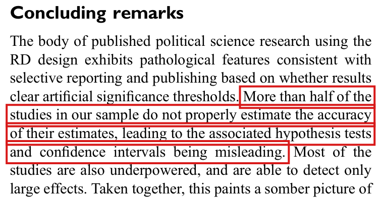
Concluding remarks, p. 10: “More than half of the studies in our sample do not properly estimate the accuracy of their estimates, leading to the associated hypothesis tests and confidence intervals being misleading.”

The problem

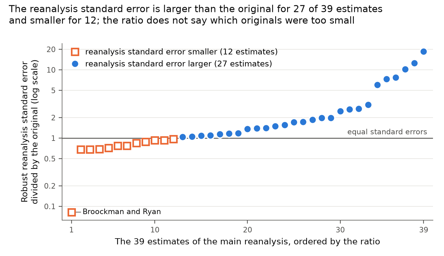
The three sentences state a diagnosis of the original studies: their methods of inference were inappropriate, their standard errors were too small, and this holds for more than half of the 45 studies in the sample. The paper supports the diagnosis with a comparison. It estimates 39 effects from 25 studies again with the default settings of rdrobust, and it compares the new standard errors and tt-statistics with the published ones. The robust standard error of the reanalysis exceeds the original standard error for 27 of the 39 estimates, the absolute tt-statistic is smaller for 28, and the number of estimates above 1.961.96 falls from 30 to 18.

This comparison is between two estimators. To assess whether an original interval was appropriate for the RD argument, I need to assess its bias and sampling distribution, reported standard error and critical value under the maintained smoothness assumptions and any additional justified restrictions. Exact coverage at linear conditional means does not establish validity under those broader assumptions. The reanalysis changes the estimator and the bandwidth, adds a bias correction whose noise enters the standard error, and uses no covariates. These changes affect sampling variance. The finite example below has exact coverage at affine means and illustrates that variance comparison; it does not show validity across the smoothness class. Correct undersmoothing, which the paper explicitly accepts, can provide such validity without exact linearity, and a bias-corrected replacement may still have a larger standard error. The same comparison can also arise when the original interval almost never covers the effect. The comparison alone does not distinguish the two cases. This does not vindicate a method that lacks its claimed coverage guarantee under the maintained model; the paper need not establish actual curvature to criticize such a method. Its general warning about nonnegligible smoothing bias is sound. What still requires a connection to the original procedures is the empirical diagnosis and its stated prevalence.

The sentence on p. 10 needs a count. “More than half” of 45 studies means at least 23 studies with inappropriate inference. The paper does not classify the 45 studies by whether their inference is valid, and it does not say which count the sentence rests on. The relevant counts from the paper, the supplement and the replication files are listed in the second table below; none classifies inference validity. On pp. 3–4 the paper names three valid approaches: undersmoothing with conventional inference, bias correction with a standard error that accounts for it, and a worst-case adjustment for bias. If a study chose its bandwidth without an automated rule, or did not use rdrobust, it does not follow that its inference is inappropriate. Note that exactly 23 studies are coded with a non-automated bandwidth. The paper does not present this count as the basis of the sentence, and by the criteria of pp. 3–4 it does not count inappropriate inference.

The diagnosis is not shown to be false. The wording of p. 7 is evidential (“indicating”), rather than a claim that every increase in a replacement standard error proves original undercoverage. The theory and reanalysis support concern about inference that neglects smoothing bias. The descriptions of the original methods and the replacement comparisons do not establish how many original studies failed the relevant bias-control conditions, particularly the asserted majority of 45. The more limited empirical conclusion is that the reanalysis is consistent with understated uncertainty.

Evidence a derivation

The evidence is a derivation with exact examples, a comparison under bounded curvature and undersmoothing, a recalculation of the counts from the results saved in the replication files, and a check of the pages.

For the example, let the running variable XX be uniform on (−5,5)(-5,5) with a sharp cutoff at 00, and let Yi(0)=2+Xi+εiY_i(0)=2+X_i+\varepsilon_i and Yi(1)=6+Xi+εiY_i(1)=6+X_i+\varepsilon_i, where the errors εi\varepsilon_i are independent N(0,1)N(0,1), independent of the scores, and their variance is known. The RD effect is 44. I condition on eight observations with scores ±1,±2,±3,±4\pm1,\pm2,\pm3,\pm4 and compare three estimators. Each is the difference between a fitted intercept on the right and a fitted intercept on the left. The estimator GG fits a line to the four points on each side. The estimator LL is local linear with the triangular kernel and bandwidth 44. The estimator RR subtracts from LL an estimate of its bias from a quadratic fit with the same kernel and bandwidth. With the points on one side ordered by their distance 1,2,3,41,2,3,4 from the cutoff, the intercept weights of GG, LL and RR are

g=(1, 1/2, 0, −1/2),l=(3/2, 0, −1/2, 0),r=(3, −3, 1, 0).g=(1,\,1/2,\,0,\,-1/2),\qquad l=(3/2,\,0,\,-1/2,\,0),\qquad r=(3,\,-3,\,1,\,0).

Each vector of weights sums to 11 and has first moment 00, which implies that each estimator is unbiased for 44. Since the errors are independent with variance 11, I have

Var⁡(G)=2∑igi2=3,Var⁡(L)=2∑ili2=5,Var⁡(R)=2∑iri2=38.\operatorname{Var}(G)=2\sum_i g_i^2=3,\qquad \operatorname{Var}(L)=2\sum_i l_i^2=5,\qquad \operatorname{Var}(R)=2\sum_i r_i^2=38.

Each estimator is a linear combination of independent normal errors. I conclude that (G−4)/3(G-4)/\sqrt3, (L−4)/5(L-4)/\sqrt5 and (R−4)/38(R-4)/\sqrt{38} are standard normal. For each of the three, the interval that extends z.975z_{.975} standard errors on either side of the estimate covers the effect with probability exactly 0.950.95 at these specified affine conditional means and conditional on the eight scores. The standard error rises from 1.731.73 to 2.242.24 to 6.166.16, with pointwise coverage unchanged. For the outcomes with errors (1/10,−1/10,1/10,−1/10)(1/10,-1/10,1/10,-1/10) on each side, all three estimates equal 44, and the squared tt-statistics are 16/316/3, 16/516/5 and 8/198/19. Since 16/3>(1.96)2=2401/625>16/5>8/1916/3>(1.96)^2=2401/625>16/5>8/19, the first estimate is significant at 1.961.96 and the two replacements are not.

The example: three estimators of an RD effect equal to 4, each with 95% coverage at the specified affine means; no coverage guarantee over a smoothness class is asserted.
EstimatorVarianceStandard errorCoverageSquared tt
GG: linear fit on each side331.731.730.950.9516/3=5.3316/3=5.33
LL: local linear, bandwidth 44552.242.240.950.9516/5=3.2016/5=3.20
RR: LL with bias correction38386.166.160.950.958/19=0.428/19=0.42
Threshold (1.96)2(1.96)^23.843.84

For the opposite case, I define ψ(x)=(x2−1)(x2−4)(x2−9)(x2−16)/576\psi(x)=(x^2-1)(x^2-4)(x^2-9)(x^2-16)/576. This polynomial vanishes at the eight scores, and ψ(0)=1\psi(0)=1. Let the mean of Y(1)Y(1) be 6+x+20ψ(x)6+x+20\psi(x) instead. The effect is now 2424, and the distribution of the eight outcomes is unchanged, so that the three estimates, their standard errors and the comparison between them are unchanged. The interval G±1.963G\pm1.96\sqrt3 covers 2424 only if ∣G−4∣>16|G-4|>16. By Chebyshev’s inequality, this event has probability at most 3/2563/256. The comparison is the same in the two cases. Coverage is exactly 95%95\% at the first, affine pair of means and at most 1.2%1.2\% at the second pair. These pointwise calculations show different actual coverage, not a coverage guarantee over a common smoothness class. Even a small quadratic perturbation, E[Y(1)∣X=x]=6+x+ax2\mathbb{E}[Y(1)\mid X=x]=6+x+ax^2 with a>0a>0, biases GG by −5a-5a. At a=1/10a=1/10 its conditional coverage is about 0.94040.9404, although the curvature is only 1/51/5. Exact coverage at the affine means therefore cannot rebut the paper’s smoothness-based criticism.

A further example concerns covariates. Suppose that observed covariates Zi∼N(0,3)Z_i\sim N(0,3), independent across observations and of the scores and errors, enter both potential outcomes with known coefficient 11. Then the estimator GG applied to Y−ZY-Z has variance 33, and applied to YY it has variance 1212. Both intervals have exact coverage at the stipulated covariate and affine data-generating process, and omitting the adjustment doubles the standard error. This does not establish validity for an original study under its maintained assumptions. The main call to rdrobust in the replication files passes no covariates, and the original estimate of Gerber and Hopkins (2011) is coded there as adjusted for covariates.

There is also a comparison with valid inference over a smoothness class. Take scores x+,j=j/nx_{+,j}=j/n and x−,j=−j/nx_{-,j}=-j/n, j=1,…,nj=1,\ldots,n, independent N(0,1)N(0,1) errors of known variance, and twice differentiable conditional means with ∣md′′(x)∣≤M|m_d''(x)|\le M for a fixed finite MM. Put m=⌊n3/4⌋m=\lfloor n^{3/4}\rfloor and h=(m+1)/nh=(m+1)/n. Let AA be the local linear difference at the cutoff, using the first mm observations on each side with triangular weights 1−j/(m+1)1-j/(m+1). Let BB subtract its estimated quadratic Taylor bias using the same bandwidth and kernel. The weighted normal equations make BB the difference of the local quadratic intercepts.

For u=j/(m+1)u=j/(m+1), the limiting intercept weight functions are

K1(u)=(6−12u)(1−u),K2(u)=(12−60u+60u2)(1−u).K_1(u)=(6-12u)(1-u),\qquad K_2(u)=(12-60u+60u^2)(1-u).

Their squared integrals are 24/524/5 and 72/772/7. Both fits reproduce constants and lines and have bounded sums of absolute intercept weights, so Taylor’s theorem bounds each effect estimator’s bias by a constant times Mh2Mh^2. Their variances are asymptotic to 2(24/5)/m2(24/5)/m and 2(72/7)/m2(72/7)/m. Thus the absolute bias divided by its standard deviation is O(h2m)=O(n−1/8)O(h^2\sqrt m)=O(n^{-1/8}), uniformly over the stated mean class. The centered noise is exactly normal, so both conventional intervals have coverage tending uniformly to 0.950.95. Yet Var⁡(B)/Var⁡(A)→15/7\operatorname{Var}(B)/\operatorname{Var}(A)\to15/7 and the ratio of standard errors tends to 15/7≈1.464\sqrt{15/7}\approx1.464; for a fixed nonzero effect, the ratio of absolute test statistics for BB and AA tends in probability to 7/15<1\sqrt{7/15}<1. This establishes the paper’s undersmoothing exception without exact linearity. It does not reproduce any sampled study or the automatic bandwidths of rdrobust.

Counts available in the paper, the supplement and the replication files. “More than half” of the sample requires 23 of 45 studies with inappropriate inference.
ItemCountBasis
Studies coded with the CCT bandwidth12 of 45a choice of bandwidth
Studies coded with an IK or cross-validated bandwidth10 of 45a choice of bandwidth
Studies coded with a non-automated bandwidth23 of 45a choice of bandwidth
Studies in the main reanalysis25 of 45data available, not coded CCT
Estimates with a larger robust standard error27 of 39estimates, not studies
Estimates with a smaller absolute tt-statistic28 of 39estimates, not studies
Studies with a larger robust standard error16 of 25one main estimate per study
Estimates above 1.961.96: original, reanalysis30, 18 of 39two estimators compared

The 10 studies of the second row are 7 with an IK bandwidth and 3 with a cross-validated one, and the 23 studies of the third row include 4 with a global polynomial specification. Weighting each study equally, the mean standardized standard error rises from 0.1880.188 to 0.2650.265 and the mean absolute tt-statistic falls from 5.035.03 to 3.913.91. The count of 16 studies holds for the main estimate of each study and for the mean ratio within a study, with different sets of 16. With the conventional standard error at the same bandwidth, the counts are 21 of 39 estimates and 12 of 25 studies.

The examples do not represent any study in the sample or the data-driven defaults of rdrobust. I did not examine the original articles or their code. The pointwise affine calculations do not validate the original methods under the paper’s smoothness assumptions, and the undersmoothing derivation does not show that the sampled studies used suitable bandwidths. The replacement comparison does not identify which original procedures failed their claimed coverage conditions or establish the asserted majority.

What survives

The descriptive comparison of the saved results stands: the counts 27 of 39 and 28 of 39, the fall from 30 to 18 estimates above 1.961.96, and the larger standardized standard errors on average. The reading that this pattern is consistent with understated uncertainty survives. The general warning about nonnegligible smoothing bias on pp. 3–4 remains sound, as do the three valid routes to inference described there. The bunching of tt-statistics, the caliper tests and the power analysis do not use the disputed prevalence claim. What changes is the empirical diagnosis in the abstract: it is qualified as a concern supported by the theory and the comparison, and the undocumented share “more than half” is withdrawn. The counts above use the saved values, including the erroneous Broockman and Ryan standard error addressed in P033-N011.

Corrected

Abstract, p. 1: “However, conventional RD inference that neglects nonnegligible smoothing bias can be misleading under the usual smoothness assumptions. A standardized reanalysis often produces larger estimated standard errors and smaller absolute test statistics than the original analyses. This pattern is consistent with understated uncertainty in the original findings, but it does not by itself establish that the original inference was inappropriate.”

Results, p. 7: “Here, we see a clear shift to the left. This pattern is consistent with understated uncertainty in the original studies, but changes in the estimator, the bandwidth and the precision of the bias estimate also affect it; the comparison alone does not establish that the original analyses were miscalibrated.”

Concluding remarks, p. 10: “In our standardized reanalysis of 25 studies, the robust standard error exceeds the original standard error for 27 of 39 estimates, and the absolute test statistic is smaller for 28 of 39. Standardized standard errors are larger and absolute test statistics smaller on average. This pattern is consistent with understated uncertainty in the original studies, but the comparison alone does not establish inappropriate original inference or the fraction of studies with misleading hypothesis tests and confidence intervals.”

The sentence of the introduction that draws the same inference (p. 2, “This indicates that the body of published RD studies tends to systematically overestimate the accuracy of their findings”) takes the same qualification: “This is consistent with a tendency of the body of published RD studies to systematically overestimate the accuracy of their findings, but does not establish it.”
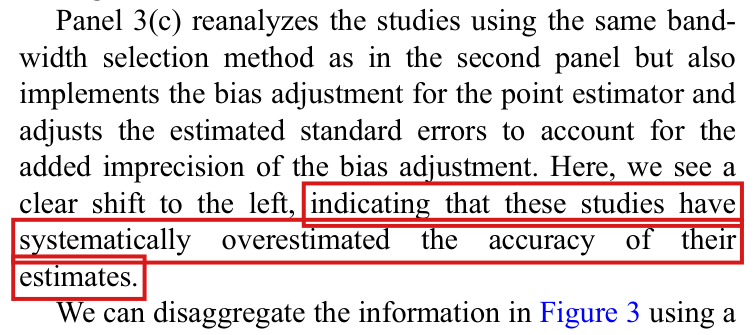

Crop of the paragraph on panel 3(c). A red outline marks the words 'indicating that these studies have systematically overestimated the accuracy of their estimates.' at the end of the paragraph.
Results, p. 7 (PDF p. 7), right column. The marked clause draws the inference from the shift in panel 3(c) to the accuracy of the original studies.
Crop of the last five lines of the abstract. A red outline marks the sentence 'However, researchers tend to use inappropriate methods for inference, rendering standard errors artificially small.'
Abstract, p. 1 (PDF p. 1). The marked sentence states the diagnosis of the original studies.
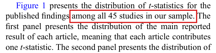
Crop of the first paragraph of the concluding remarks. A red outline marks the sentence 'More than half of the studies in our sample do not properly estimate the accuracy of their estimates, leading to the associated hypothesis tests and confidence intervals being misleading.'
Concluding remarks, p. 10 (PDF p. 10), right column. The marked sentence gives the share of studies.
Scatter plot on a logarithmic vertical axis. The 39 estimates are ordered by the ratio of the robust reanalysis standard error to the original standard error. Twelve open orange squares lie below the horizontal line at ratio 1: eleven between about 0.68 and 0.97, and one, labelled Broockman and Ryan, at 0.08. Twenty-seven blue circles lie above the line, rising from just above 1 to about 18.
The comparison behind the three sentences, from the results saved in the replication files: for each of the 39 estimates of the main reanalysis, the robust standard error of the reanalysis divided by the original standard error. The lowest point is the estimate of Broockman and Ryan (2016), whose reanalysis standard error is corrected in P033-N011.
My comment and the history of this entry

I disagree that this is an error. This is an implication of the motivation of the study. The implication is that the RD design is motivated by the semiparametric continuity assumption, not by stronger (e.g., linearity) assumptions. Thus, under those implicit (smoothness-only) conditions, the inference procedures used were inappropriately optimistic.

Updated after the LLM decision: I continue to believe this is a clarity note, not a major error. I think this is an example of the (current) LLMs being overly literal in interpretation.

Suggested classification: clarity note.

My position My comment above; I suggested a clarity note.

The models’ position Smoothness also permits valid undersmoothing, and comparing standard errors does not establish which procedures the original studies used, or that a majority of the 45 articles used inference inappropriate under that standard. The diagnosis is central to the paper: Major.

  1. Classification before my review (the classification when the audit was first completed, before I reviewed it): Major error.
  2. I commented and suggested a clarity note.
  3. Independent evaluation. Incorporated in part. The entry now acknowledges the paper’s standard of continuity and smoothness and its warning about neglected bias, and qualifies the coverage claims of its affine example as pointwise. My suggested classification (clarity note) was not adopted.

Moderate (2)

A real substantive error with limited reach.

For Coppock and Green (2016), the estimate is an effect on the probability of voting but is standardized by the standard deviation of counts of voters, so that its “d=0.1d=0.1” is not Cohen’s dd for the individual voting contrast; under the paper’s normal approximation with the saved standard error, the study cannot reach 95% power at d=0.1d=0.1.

Power analysis, p. 9 (PDF p. 9), left column; Table 2, p. 9, row 0.1; Table 3, p. 10 (PDF p. 10), panel “Studies not using election data”, row 0.1

See also under Formal statements (Lean): P033-T5, P033-T6, P033-T17, P033-T18

I disputed this classification, but as a rule, deferred to the models’ final judgment: see my comment and the history of this entry.

As printed

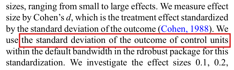
p. 9: “We measure effect size by Cohen’s dd, which is the treatment effect standardized by the standard deviation of the outcome (Cohen, 1988). We use the standard deviation of the outcome of control units within the default bandwidth in the rdrobust package for this standardization.”

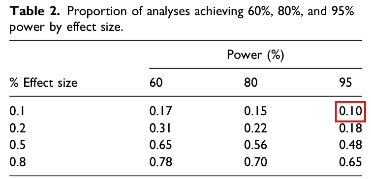
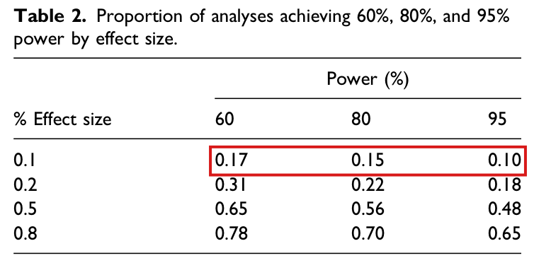
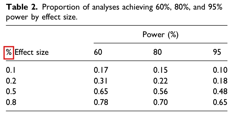
Table 2, p. 9, row 0.1 (power 60, 80, 95): 0.17, 0.15, 0.10.

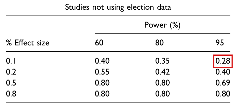
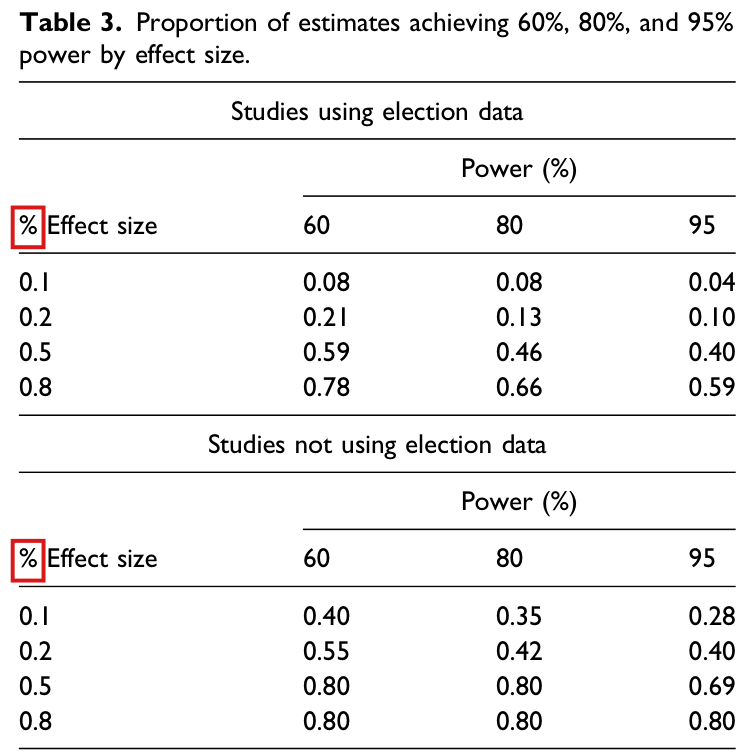
Table 3, p. 10, studies not using election data, row 0.1: 0.40, 0.35, 0.28.

The problem

The definition is right in general. For Coppock and Green, the code accurately computes an outcome-standardized aggregate fuzzy-IV coefficient per additional prior voter, a different comparison from Cohen’s dd for individual turnout. In the analysis file for Coppock and Green (2016), each of the 140,659 rows is an aggregate: the outcome and the treatment are counts of voters, with maxima 294 and 552. The reanalysis is a fuzzy RD of one count on the other. Its estimate, 0.0660.066 with robust standard error 0.01550.0155, is a ratio of two discontinuities in counts. This is an aggregate outcome-count slope per prior voter; under the scientific interpretation in the paper’s study metadata, the ratio identifies an effect on an individual’s probability of voting. The code divides this effect by the standard deviation of the counts, 24.5824.58 within the bandwidth for the power analysis and 41.6641.66 below the cutoff for the funnel plots. The code’s d=0.1d=0.1 passes an alternative of 2.462.46 to the fuzzy-RD slope calculation, and the saved power equals 11 at all four effect sizes. That value is consistent with the code-defined target and saved standard error; the mismatch concerns its interpretation as individual Cohen’s dd. The divisor also depends on the size of the aggregates: at fixed bandwidths, doubling every count leaves the effect and its standard error unchanged and doubles the divisor.

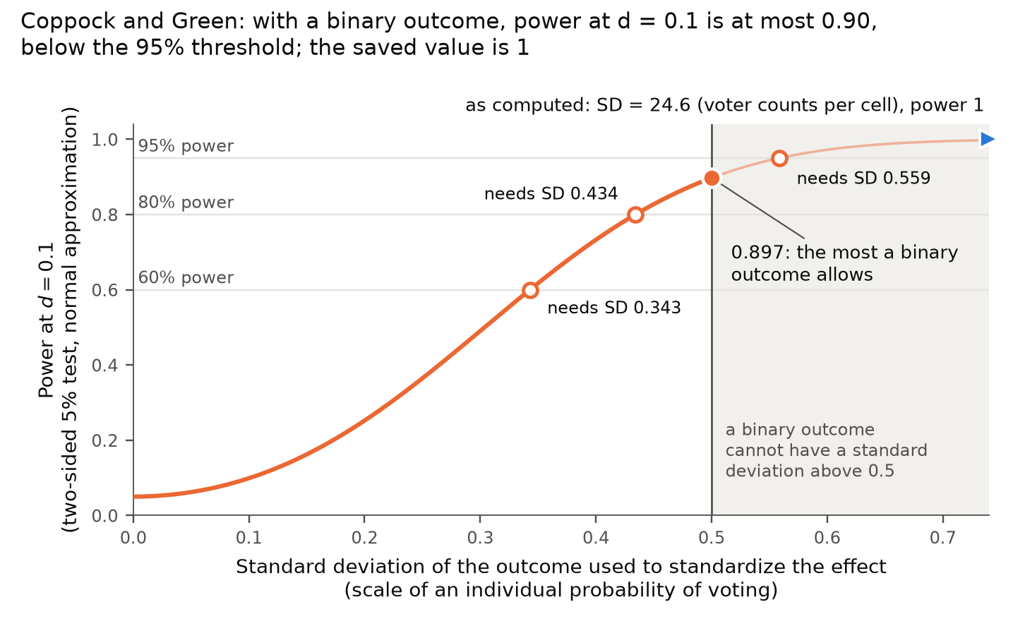
For the intended individual voting contrast, the outcome is binary and its population standard deviation is at most 1/21/2. An effect size of d=0.1d=0.1 is then an effect of at most 0.050.05, and under the normal approximation of the paper, with the saved robust standard error, the power at d=0.1d=0.1 is at most about 0.89730.8973. Under this approximation, the study cannot attain 95% power at d=0.1d=0.1, and one cell in each of Tables 2 and 3 changes. Whether the study attains 60% or 80% power at d=0.1d=0.1 depends on the standard deviation of individual turnout, which the analysis file does not contain. The code also takes the observations to the left of the cutoff as the control units. In this file the treatment is concentrated on the left: within 200 days of the cutoff its mean is 100.7100.7 on the left and 0.420.42 on the right. The left side is not a group of untreated individuals.

Evidence an exact counterexample

The evidence is an exact counterexample to interpreting the code-defined standardization as individual Cohen’s dd, a recalculation from the replication files, and a bound on power for that individual target.

The counterexample has two types of cell on each side of an eligibility cutoff. The two types are equally likely, and each cell has 100 individuals. On the eligible side, each cell has 50 voters in the earlier election, and the two types have 10 and 50 voters in the later one; five of the earlier voters in each cell are induced to vote later, so the later-voter counts without treatment would be 5 and 45. On the ineligible side, no one voted in the earlier election, and the two types have 10 and 40 voters in the later one. The fuzzy RD effect is (30−25)/(50−0)=1/10(30-25)/(50-0)=1/10. Turnout without treatment is 1/41/4 on each side, with variance 3/163/16, and Cohen’s dd satisfies d2=(1/10)2/(3/16)=4/75d^2=(1/10)^2/(3/16)=4/75. The sample variance of the counts on the eligible side is (10−30)2+(50−30)2=800(10-30)^2+(50-30)^2=800, and the standardization of the replication files gives d2=(1/10)2/800=1/80000d^2=(1/10)^2/800=1/80000. Doubling the population and the counts of every cell leaves the effect at 1/101/10 and Cohen’s d2d^2 at 4/754/75. The variance of the counts becomes 32003200, and the second quantity becomes 1/3200001/320000.

For the bound, a binary outcome with mean pp has variance p−p2≤1/4p-p^2\le1/4. Let ss be the saved robust standard error (approximately 0.01550.0155) and z=z.975z=z_{.975}. Under the normal approximation, the power at d=0.1d=0.1 with standard deviation σ\sigma is

Φ(μ−z)+Φ(−μ−z),μ=0.1 σ/s,\Phi(\mu-z)+\Phi(-\mu-z),\qquad \mu=0.1\,\sigma/s,

which increases in μ≥0\mu\ge0. Substituting σ=1/2\sigma=1/2, I obtain approximately 0.89730.8973. Solving for the standard deviations such that the power equals 60%, 80% and 95%, I find approximately 0.3430.343, 0.4340.434 and 0.5590.559. The last exceeds 1/21/2. A sample standard deviation with divisor N−1N-1 can exceed 1/21/2 slightly. For a control group that contains all untreated later-election voters in the cells to the right of the cutoff within the bandwidth, at least 31,731 individuals, the bound is approximately 0.897270.89727.

A fit of rdrobust version 2.2 to the analysis file reproduces the saved coefficient and robust standard error to within 10−810^{-8}, with bandwidth 105.66105.66 days; the original code used version 2.1.1. The local count standard deviation is 24.5795462324.57954623, so the code-defined target at d=0.1d=0.1 is 2.457954622.45795462. These reproduce the alternative actually computed, not individual Cohen’s dd. At the same bandwidths, doubling every count leaves the coefficient and its standard error unchanged. The study is one of the ten studies that do not use election data and has weight 11. Changing its indicator for 95% power at d=0.1d=0.1 from 11 to 00 changes the two cells as follows.

The two cells at effect size 0.1 and power 95%, with only this study changed.
CellAs printedCorrected
Table 25/48≈0.1045/48\approx0.10411/144≈0.07611/144\approx0.076
Table 3, studies not using election data11/40=0.27511/40=0.2757/40=0.1757/40=0.175

The bound holds for the normal approximation with the saved standard error. It is not a statement about the exact power of the test in finite samples. I take the saved powers from the replication files; I have not independently executed rdpower.

What survives

The estimate itself, its standard error, its tt-statistic and its pp-value do not use the standardization, and the histograms of tt-statistics and the caliper tests are unchanged. A common divisor cancels in the ratio of an estimate to its standard error, so that the study stays on the same side of the significance line in the funnel plots. What changes is its row of the power analysis and its position on the common scale of Figures 4, S4, S7 and S8. In panel (a) of Figure 4 it is plotted at about (0.002,0.00005)(0.002,0.00005). The advantage of studies without election data at d=0.1d=0.1 becomes smaller and keeps its sign. If this study also failed the 60% and 80% thresholds, the proportions would be 0.300.30 and 0.250.25, against 1/13≈0.081/13\approx0.08 for election studies. Replacing the code-defined power of 11 with power for the individual Cohen-dd target reinforces the conclusion that the studies are underpowered. The correction of P033-N011 lowers the same cell of Table 2 for another study; each value here applies one correction alone.

Corrected

p. 9: “We measure effect size by Cohen’s dd, which is the treatment effect standardized by the standard deviation of the outcome (Cohen, 1988). We use the standard deviation of the outcome of control units within the default bandwidth in the rdrobust package for this standardization, with the outcome and effect referring to the same treatment contrast. For Coppock and Green (2016), the intended contrast is an effect on an individual’s probability of voting, so that the standard deviation needed is that of individual turnout among control units. The earlier code instead standardized an aggregate fuzzy-IV slope per prior voter by the standard deviation of outcome counts. That statistic is reproducible but does not give individual Cohen’s dd. Individual Cohen’s dd cannot be computed from the replication data, and we report this study’s standardized effect sizes as unavailable. Since the population standard deviation of a binary outcome is at most 1/21/2, the study does not attain 95% power at d=0.1d=0.1 under the normal approximation with the saved robust standard error.”

Table 2, row 0.1: 0.17, 0.15, 0.08.

Table 3, studies not using election data, row 0.1: 0.40, 0.35, 0.175, which is about 0.180.18.

The retained entries 0.170.17 and 0.400.40 are conditional on the study attaining 60% power at d=0.1d=0.1; 0.150.15 and 0.350.35 are conditional on its attaining 80% power. Under the same approximation, the respective standard deviations of individual turnout required are approximately 0.3430.343 and 0.4340.434.

Crop of the paragraph that defines effect size by Cohen's d. A red outline marks the words 'the standard deviation of the outcome of control units'.
Power analysis, p. 9 (PDF p. 9), left column. The marked words name the standard deviation used to standardize the effect.
Crop of Table 2. A red outline marks the cell 0.10 in the row for effect size 0.1 and the column for power 95.
Table 2, p. 9 (PDF p. 9). The marked cell is the share of analyses with 95% power at effect size 0.1.
Crop of the second panel of Table 3, 'Studies not using election data'. A red outline marks the cell 0.28 in the row for effect size 0.1 and the column for power 95.
Table 3, p. 10 (PDF p. 10), panel “Studies not using election data”. The marked cell is the share with 95% power at effect size 0.1.
Line chart. The horizontal axis is the standard deviation of the outcome on the scale of an individual probability of voting, from 0 to 0.74; the vertical axis is power at d = 0.1, from 0 to 1. The curve rises from 0.05 at zero to 0.897 at a standard deviation of 0.5, where a vertical line marks the largest population standard deviation of a binary outcome; the region beyond is shaded. Open circles on the curve mark standard deviations 0.343, 0.434 and 0.559, needed for 60, 80 and 95 percent power. A blue arrow at the top right marks the value as computed in the replication files: standard deviation 24.6 (voter counts per cell), power 1.
Power at d=0.1d=0.1 for Coppock and Green (2016) under the normal approximation of p. 9, as a function of the standard deviation that standardizes the effect, with the robust standard error held at its saved value (approximately 0.01550.0155). Open circles mark the standard deviations needed for 60%, 80% and 95% power.
My comment and the history of this entry

I think this is minor. It's accurate as-coded even if not on the authors' original scale.

Suggested classification: Minor error.

My position My comment above; I suggested a Minor error.

The models’ position The slope is a different contrast from the individual Cohen’s d that the paper presents, and using it changes a power classification and summary comparisons: Moderate.

  1. Classification before my review (the classification when the audit was first completed, before I reviewed it): Moderate error.
  2. I commented and suggested a Minor error.
  3. Independent evaluation. Incorporated in part. The entry now says that the code accurately computes the standardized slope that it targets, and describes a mismatch of comparisons rather than an arithmetic error. My suggested rating (Minor) was not adopted.

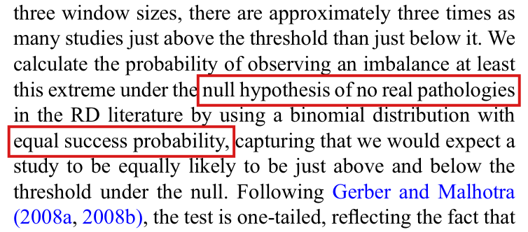
With the default variance of rdrobust and clustering, a cell of at least four observations that share a value of the running variable inside one cluster adds nothing to the variance; the reanalysis standard error of Broockman and Ryan (2016) and its saved power of 11 come from this cancellation, and correcting that study alone under the normal approximation turns the 17% of p. 9 into about 14%.

Table 2, p. 9 (PDF p. 9), row 0.1, and the sentence on 17% of the analyses; Table 3, p. 10 (PDF p. 10), panel “Studies using election data”, row 0.1; reanalysis method, p. 7 (PDF p. 7)

See also under Formal statements (Lean): P033-T3, P033-T4, P033-T17

My comment on this entry

As printed

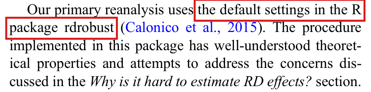
p. 7: “Our primary reanalysis uses the default settings in the R package rdrobust (Calonico et al., 2015).”

Table 2, p. 9, row 0.1 (power 60, 80, 95): 0.17, 0.15, 0.10.

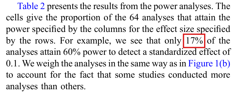
p. 9: “For example, we see that only 17% of the analyses attain 60% power to detect a standardized effect of 0.1.”

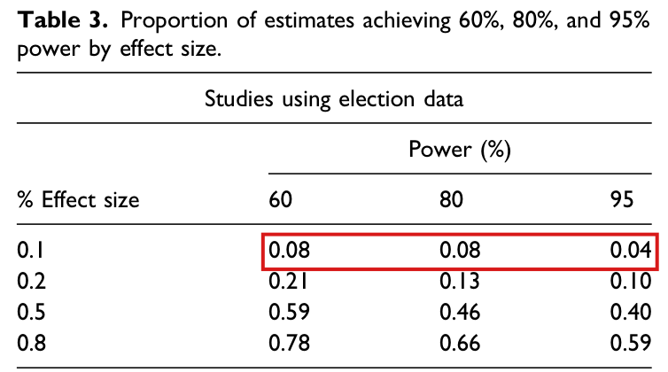
Table 3, p. 10, studies using election data, row 0.1: 0.08, 0.08, 0.04.

The problem

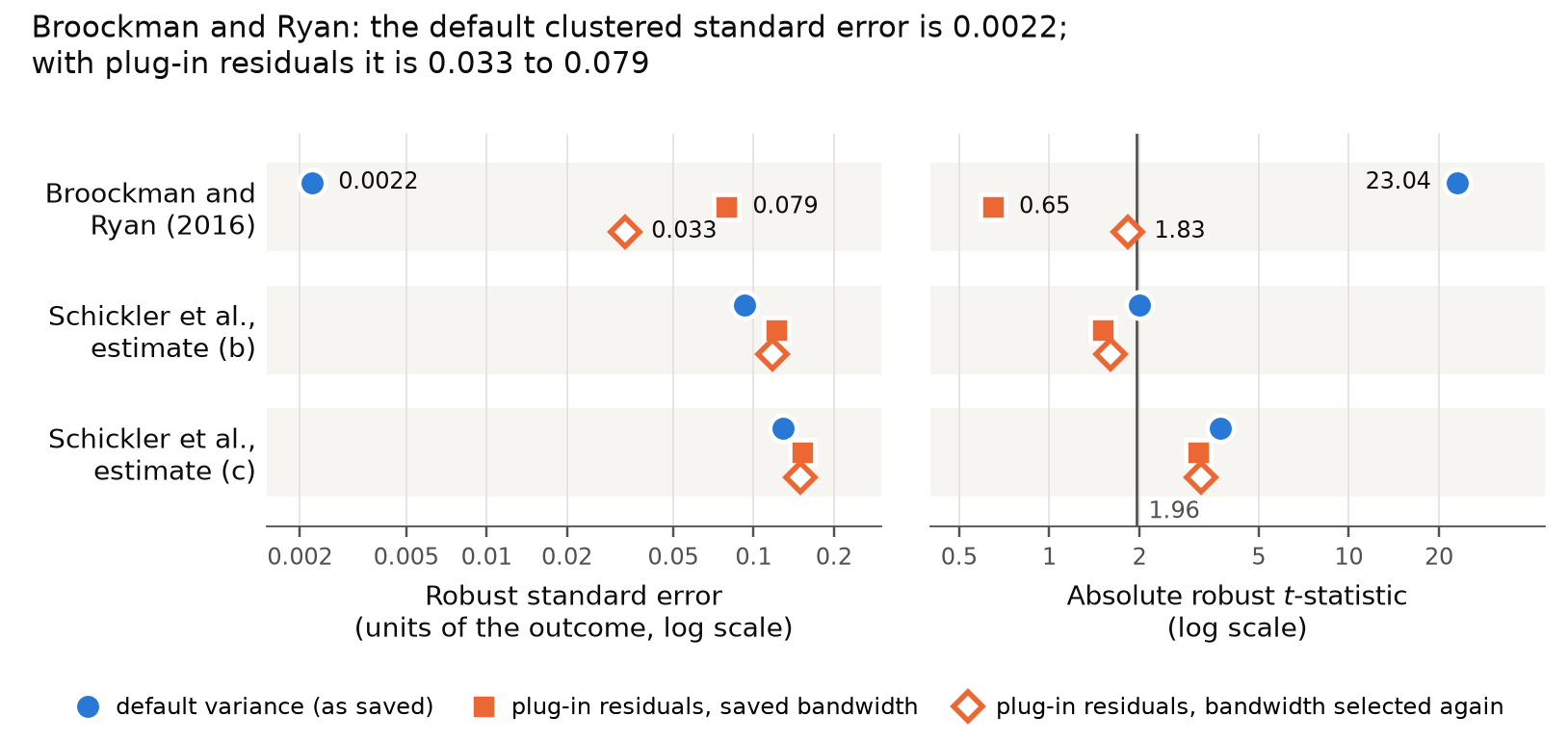
The reanalysis calls rdrobust with the cluster variable of each study and the default variance estimator, which is built from nearest-neighbour residuals. The cancellation arises in the package’s documented default combination of nearest-neighbour residuals and clustering, inherited through the paper’s ordinary call; the paper did not independently write the cancelling variance formula. I call a set of observations with the same value of the running variable a cell. When a cell has m≥4m\ge4 observations, the neighbours of each observation are the other m−1m-1 members of the cell. The residual of an observation is then m/(m−1)\sqrt{m/(m-1)} times the deviation of its outcome from the mean of the cell. For any values of the outcomes, these residuals sum to zero over the cell. The regression weights depend only on the running variable and are constant on the cell. A cell that lies inside one cluster then contributes zero to the score of that cluster. The uncertainty shared by the members of the cluster is left out of the variance. If every cell in the estimation and bias bandwidths has at least four observations and lies inside one cluster, the estimated variance is zero for the conventional and for the bias-corrected estimator.

The data of Broockman and Ryan (2016) nearly have this structure. The 29,413 survey respondents share 759 distinct values of the running variable, and the clusters are 380 districts. Inside the selected bandwidth there are 1,516 respondents in 36 cells, and 1,470 of them are in cells contained in one district. The only cell with a nonzero contribution is one of 46 respondents shared by two districts. The saved standard errors, 0.002110.00211 for the conventional estimate and 0.002220.00222 for the robust one, come from this cell alone. The reanalysis tt-statistic of 23.023.0 and the saved power of 11 at every effect size follow from them. With regression plug-in residuals in place of the nearest-neighbour residuals and the same clusters, the robust standard error is 0.07900.0790 at the saved bandwidths, with t=0.65t=0.65, and 0.03300.0330 when the bandwidths are selected again, with t=1.83t=1.83.

The paper uses the default procedure as its reanalysis benchmark. Its statement that the cited methods represent progress is a general methodological judgment and is not refuted here. The application of this default as an uncertainty benchmark needs qualification for clustered designs in which observations in a cluster share values of the running variable. The paper should have checked whether the documented default was suitable for those designs. A larger number of clusters does not remove the problem. I established the cancellation for one study of 36. Two estimates of Schickler et al., with cells of two or three observations, are sensitive to the residuals to a lesser degree. Three other clustered studies, Bohlken (2018), Gulzar and Pasquale (2017) and Larreguy et al. (2016), were not checked, since I did not have their data files.

Evidence an exact counterexample

The evidence is a derivation, an exact counterexample, and a recalculation on the data of the replication files.

Let CC be a cell of m≥4m\ge4 observations with outcomes yiy_i and sum SS. The nearest-neighbour residual of observation ii is

ri=m−1m(yi−S−yim−1)=mm−1(yi−Sm),r_i=\sqrt{\frac{m-1}{m}}\Bigl(y_i-\frac{S-y_i}{m-1}\Bigr)=\sqrt{\frac{m}{m-1}}\Bigl(y_i-\frac{S}{m}\Bigr),

which implies that ∑i∈Cri=0\sum_{i\in C}r_i=0. The weight of an observation in the local polynomial fit depends only on its value of the running variable. The contribution of CC to the score of a cluster that contains it is this weight times ∑i∈Cri\sum_{i\in C}r_i, which is zero. The same holds for the bias-corrected estimator.

The counterexample has ten independent clusters at x=−5,…,−1,1,…,5x=-5,\dots,-1,1,\dots,5, with five observations each and cutoff 00. The estimator is local linear with a quadratic fit for the bias, the triangular kernel and bandwidths h=b=6h=b=6. Let U1,…,U10U_1,\dots,U_{10} be independent and uniform on {−1,1}\{-1,1\}, and let every observation of cluster gg have the outcome UgU_g under both treatments. The RD effect is 00. The conventional estimator equals ∑gagUg\sum_g a_gU_g with

a=(1/5, 1/5, 0, −2/5, −1, 1, 2/5, 0, −1/5, −1/5),a=(1/5,\,1/5,\,0,\,-2/5,\,-1,\,1,\,2/5,\,0,\,-1/5,\,-1/5),

and its variance is ∑gag2=62/25\sum_g a_g^2=62/25. A direct computation gives the variance 1010 for the bias-corrected estimator. Every nearest-neighbour residual is 00, and both estimated variances are 00 in all 10241024 outcomes, while the two estimates are nonzero in 912912 and 968968 of them. If independent noise, uniform on {−1,1}\{-1,1\}, is added to every observation, then the covariance matrix of each cluster is positive definite. The true variances become 372/125372/125 and 1212, and the estimated variances stay 00.

More clusters do not help. For n≥3n\ge3, I place n(n+1)n(n+1) clusters of five observations on each side at x=±j/(n(n+1))x=\pm j/(n(n+1)) and set h=b=1/nh=b=1/n, so that nn clusters on each side have positive weight. With outcome UgU_g for every observation in cluster gg, without the added observation noise, the variance of the conventional estimator is

Vn=12(4n2+5n−1)5n(n−1)(n+1),nVn→48/5,V_n=\frac{12(4n^2+5n-1)}{5n(n-1)(n+1)},\qquad nV_n\to48/5,

and the default estimate of it is 00 for all nn.

On the data of Broockman and Ryan, I find the same cancellation with exact rational arithmetic. In the union of the two bandwidth windows there are 43 cells on each side, each with at least four respondents, and all but one lie inside one district. The exception is the cell at x=0.0013536513x=0.0013536513 with 46 respondents from two districts, whose sums of deviations from the mean of the cell are +19/46+19/46 and −19/46-19/46. The sandwich formula applied to this cell alone reproduces both saved standard errors. A fit of rdrobust with the default variance reproduces the saved coefficients and standard errors of the three estimates in the figure to within 4.8×10−164.8\times10^{-16}.

For the tables, I use the power under the normal approximation, Φ(d σ0/s−z.975)+Φ(−d σ0/s−z.975)\Phi(d\,\sigma_0/s-z_{.975})+\Phi(-d\,\sigma_0/s-z_{.975}), where ss is the robust standard error with plug-in residuals and σ0\sigma_0 the standard deviation of the outcome among control units within the bandwidth. At d=0.1d=0.1 the power of the Broockman and Ryan estimate is 0.0890.089 at the saved bandwidths and 0.2940.294 with bandwidths selected again, below all three thresholds in both cases. The study has weight 11 of 36, and of 26 among election studies.

Cells that change when the Broockman and Ryan estimate alone is corrected, with every other saved power held fixed. The values are the same at the saved bandwidths and with bandwidths selected again.
Cell (effect size, power)As printedCorrectedAs a fraction
Table 2 (0.1, 60%)0.170.1395/365/36
Table 2 (0.1, 80%)0.150.1251/81/8
Table 2 (0.1, 95%)0.100.07611/14411/144
Table 2 (0.2, 95%)0.180.15311/7211/72
Table 3, election data (0.1, 60%)0.080.0381/261/26
Table 3, election data (0.1, 80%)0.080.0381/261/26
Table 3, election data (0.1, 95%)0.04000
Table 3, election data (0.2, 95%)0.100.0583/523/52

At the saved bandwidths, six further cells fall: the 60% and 80% cells at d=0.2d=0.2 and the 95% cell at d=0.5d=0.5, in Table 2 and in the election panel of Table 3. For Schickler et al., the robust standard error of estimate (b) at the saved bandwidths moves from 0.0920.092 to 0.1220.122 and its tt-statistic from 2.002.00 to 1.511.51. The robust standard error of estimate (c) moves from 0.1290.129 to 0.1530.153.

Several limits apply. The true sampling standard deviations are unknown, and the ratio of the two standard errors compares one estimator with another, not an estimator with the truth. Plug-in residuals remove the cancellation. I do not claim that the resulting intervals have correct coverage or that this is the only repair. Computing the conventional standard error by weighted least squares with errors clustered by district, I obtain 0.06300.0630 at the saved bandwidth. The rdpower package was not available, and the powers above are the normal approximation. The paper used version 2.1.1 of rdrobust and the recalculation used version 2.2, which reproduces the saved values.

What survives

The statistics reported by the original studies, the selection of studies, the bunching of the original tt-statistics and the caliper tests on those original statistics do not use the reanalysis variance. Reanalyses without this cancellation are unaffected by this finding, and so is the rdhonest reanalysis, which is restricted to studies without clustering. The Broockman and Ryan replacements lower the apparent precision and power of that reanalysis, reinforcing the conclusions on low power and on larger reanalysis standard errors. Survival of these broad conclusions does not validate the affected default as an uncertainty benchmark. What changes is the Broockman and Ryan reanalysis: its standard errors, its bandwidth, its tt-statistics, its place in panels (b) and (c) of Figures 3 and 4, and its power. With it change the first rows of Table 2 and of the election panel of Table 3, the quoted 17%, and the summaries of the supplement that use the same row. P033-E010 concerns a different defect in the same tables and changes other cells. Under the stated normal approximation, P033-N010 lowers the same 95% cell of Table 2 for another study, and each value here applies one correction alone.

Corrected

p. 7: “Our primary reanalysis uses the default settings in the R package rdrobust (Calonico et al., 2015), except for the variance in clustered designs in which observations in a cluster share values of the running variable. In such a design, the default nearest-neighbour residuals within a cell of four or more observations with the same value of the running variable sum to zero, and a cell of this kind inside one cluster contributes nothing to the cluster-robust variance. For these designs we replace those residuals, for example with regression plug-in residuals, retain the specified clusters and covariance when a cluster spans the cutoff, and propagate the change through bandwidth selection and power analysis.”

Table 2, row 0.1: 0.14, 0.13 (1/81/8 exactly), 0.08.

p. 9: “For example, we see that only 14% of the analyses attain 60% power to detect a standardized effect of 0.1.”

Table 3, studies using election data, row 0.1: 0.04, 0.04, 0.00.

These values correct the estimate of Broockman and Ryan (2016) alone, by the normal approximation with plug-in residuals, and hold every other saved power fixed. The cells at effect size 0.2 and power 95% become 0.150.15 in Table 2 and 0.060.06 in the election panel of Table 3. A full correction fits every clustered study again, including the three that were not checked here.

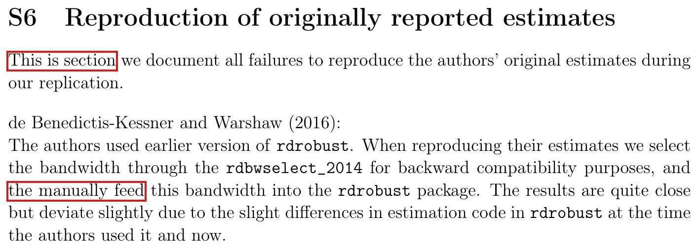
Crop of the paragraph that begins 'Our primary reanalysis uses'. A red outline marks the words 'the default settings in the R package rdrobust', which run over two lines.
Reanalysis method, p. 7 (PDF p. 7), left column. The marked words name the procedure used in the primary reanalysis.
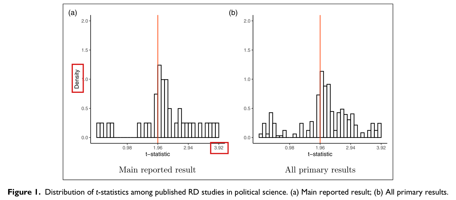
Crop of the paragraph that introduces Table 2. A red outline marks the figure 17 percent in the sentence 'For example, we see that only 17 percent of the analyses attain 60 percent power to detect a standardized effect of 0.1.'
p. 9 (PDF p. 9), left column. The marked figure is the share of analyses with 60% power at effect size 0.1.
Crop of Table 2. A red outline marks the three cells of the row for effect size 0.1: 0.17, 0.15 and 0.10.
Table 2, p. 9 (PDF p. 9). The marked row is effect size 0.1.
Crop of the first panel of Table 3, 'Studies using election data'. A red outline marks the three cells of the row for effect size 0.1: 0.08, 0.08 and 0.04.
Table 3, p. 10 (PDF p. 10), panel “Studies using election data”. The marked row is effect size 0.1.
Two dot plots side by side with logarithmic horizontal axes and three rows: Broockman and Ryan (2016), and estimates (b) and (c) of Schickler et al. Left panel, robust standard error: for Broockman and Ryan the default value is 0.0022 (blue circle), against 0.079 with plug-in residuals at the saved bandwidth (orange square) and 0.033 with bandwidths selected again (open orange diamond); for the two Schickler estimates the three values lie close together between 0.09 and 0.16. Right panel, absolute robust t-statistic with a vertical line at 1.96: for Broockman and Ryan 23.04 by default against 0.65 and 1.83; for Schickler (b) about 2.0 by default against about 1.5 and 1.6; for Schickler (c) about 3.1 to 3.7.
Robust standard error and absolute robust tt-statistic of three clustered reanalyses, under the default variance (as saved in the replication files) and with plug-in residuals, at the saved bandwidths and with bandwidths selected again.
My comment and the history of this entry

This is a problem with rdrobust that we should have noticed. It's not an error of ours per se, but it does affect one of the conclusions.

Suggested classification: Moderate error.

  1. Classification before my review (the classification when the audit was first completed, before I reviewed it): Moderate error.
  2. I commented and suggested a Moderate error.
  3. Independent evaluation. Incorporated. The entry now attributes the defect to the default settings of the rdrobust package, which the paper’s call inherited. It remains a Moderate error, as I suggested.

Minor (11)

Real but inconsequential, for example a misprint that does not change a result.

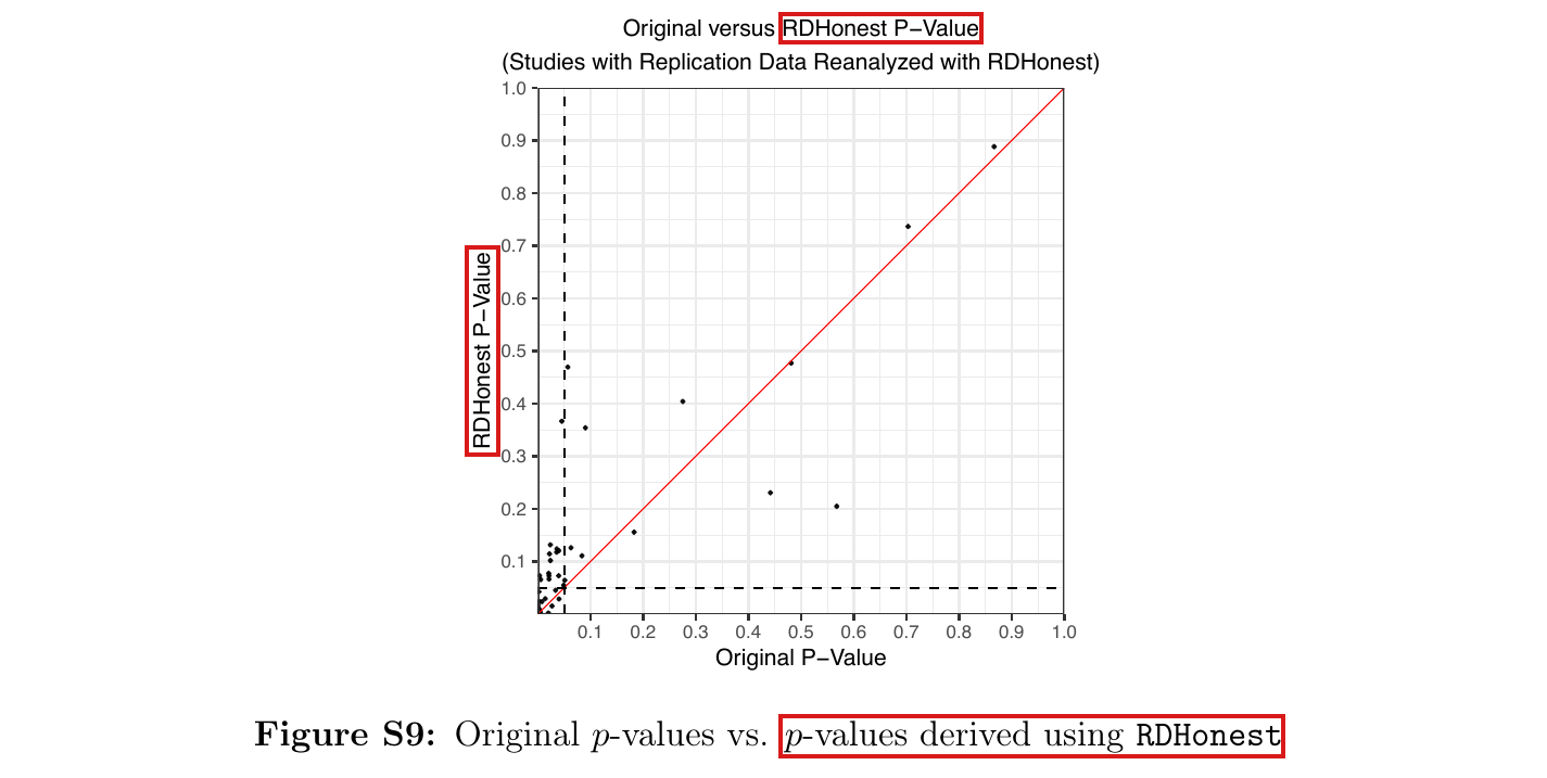
The vertical axis of Figure S9 shows a normal-tail transform of the pseudo tt-statistic built from one 95% bias-aware interval, which reproduces the 5% decision of that interval but is not in general a valid pp-value at other levels.

Supplement, Figure S9, p. 18: title, vertical-axis label and caption

See also under Formal statements (Lean): P033-T12, P033-T13

As printed

Title: “Original versus RDHonest P-Value”. Subtitle: “(Studies with Replication Data Reanalyzed with RDHonest)”. Horizontal axis: “Original P-Value”. Vertical axis: “RDHonest P-Value”.

Caption: “Figure S9: Original pp-values vs. pp-values derived using RDHonest”.

The problem

The quantity on the vertical axis is not a pp-value returned by the RDHonest procedure. Let θ^\widehat\theta be the RDHonest estimate, let hh be the half-length of its 95% bias-aware confidence interval, and write z=Φ−1(0.975)z=\Phi^{-1}(0.975). The replication code computes the pseudo standard error h/zh/z and the pseudo tt-statistic z∣θ^∣/hz|\widehat\theta|/h, and it plots

p∗=2Φ(−z∣θ^∣/h).p_*=2\Phi\bigl(-z|\widehat\theta|/h\bigr).

The main text (p. 8) and Section S9 call the tt-statistics “pseudo”, but the title, the axis label and the caption of Figure S9 call p∗p_* a pp-value without qualification. A pp-value PP for a null hypothesis must satisfy Pr⁡(P≤α)≤α\Pr(P\le\alpha)\le\alpha under the null for every level α\alpha. The rule p∗<0.05p_*<0.05 rejects exactly when the interval excludes zero. This implies that the rule has level at most 5% when the interval has 95% coverage. At other levels p∗p_* need not satisfy the requirement, as the example below shows.

Evidence an exact counterexample

This correction rests on a derivation, an exact counterexample and a comparison with the replication files. I checked the Figure S9 labels in the released figure and the caption in the supplement’s extracted text; I did not have the typeset supplement page. Since Φ\Phi is strictly increasing, I have for every h>0h>0 that

p∗<0.05  ⟺  2Φ(−z∣θ^∣/h)<2Φ(−z)  ⟺  ∣θ^∣>h  ⟺  0∉[θ^−h,θ^+h].p_*<0.05\iff 2\Phi\bigl(-z|\widehat\theta|/h\bigr)<2\Phi(-z)\iff|\widehat\theta|>h\iff 0\notin[\widehat\theta-h,\widehat\theta+h].

For the counterexample, let T∼N(θ+b,1)T\sim N(\theta+b,1), where the bias bb satisfies ∣b∣≤B|b|\le B for a known bound B=1B=1. Let HH be the unique positive number such that

Φ(H−B)−Φ(−H−B)=1920.\Phi(H-B)-\Phi(-H-B)=\frac{19}{20}.

The interval [T−H,T+H][T-H,T+H] covers θ\theta with probability at least 19/2019/20 for every θ\theta and every ∣b∣≤B|b|\le B, with equality at b=±Bb=\pm B. Applied to this interval, the transform is p∗(T)=2Φ(−z∣T∣/H)p_*(T)=2\Phi(-z|T|/H). Fix θ=0\theta=0, b=1b=1 and α=1/5\alpha=1/5, and set q=Φ−1(9/10)q=\Phi^{-1}(9/10) and C=Hq/zC=Hq/z. Then p∗≤1/5p_*\le 1/5 exactly when ∣T∣≥C|T|\ge C, and since T∼N(1,1)T\sim N(1,1), I have

Pr⁡(p∗≤1/5)=Φ(1−C)+Φ(−1−C).\Pr(p_*\le 1/5)=\Phi(1-C)+\Phi(-1-C).

In exact rational arithmetic, I find that 2.64614554821530<H<2.646145548215402.64614554821530<H<2.64614554821540 and that

0.23579196727091<Pr⁡(p∗≤1/5)<0.23579196727101.0.23579196727091<\Pr(p_*\le 1/5)<0.23579196727101.

The transform therefore rejects a true null about 23.6% of the time at the nominal 20% level, although the worst-case coverage of the interval is exactly 95%. With B=b=1/2B=b=1/2 the same probability exceeds 0.204149056327650.20414905632765. At α=1/20\alpha=1/20 the rejection probability is exactly 1/201/20.

The 46 values plotted in Figure S9 agree with this transform of the stored pseudo tt-statistics to within 1.3×10−151.3\times 10^{-15}. For each of them, p∗<0.05p_*<0.05 agrees with the 95% interval excluding zero, which 20 of the 46 intervals do. I have not established the rejection rates of the transform for the 46 estimates themselves. When there is no bias, so that B=0B=0 and H=zH=z, the transform is the ordinary two-sided normal pp-value at every level.

What survives

No plotted number, interval or 5% decision changes. The pseudo tt-statistics and pseudo standard errors of Figures S5 to S8 and Table S6 are as the paper describes them. The rdrobust results, the caliper tests and the power tables use other quantities, and Figure S9 is the only place where these values are used. The reading of the full vertical scale of Figure S9, and of its diagonal, as a comparison of pp-values does change.

Corrected

Title: “Original p-values versus RDHonest pseudo p-values”. Vertical axis: “RDHonest pseudo p-value”.

Caption: “Figure S9: Original pp-values versus normal-tail transforms of RDHonest pseudo tt-statistics. The vertical quantity is p∗=2Φ(−z0.975∣θ^∣/h)p_*=2\Phi(-z_{0.975}|\widehat\theta|/h), where hh is the reported 95% bias-aware confidence-interval half-length. The rule p∗<0.05p_*<0.05 is exactly equivalent to this interval excluding zero. These transforms are not generally valid pp-values at other significance levels; any 5% validity inherits the interval’s coverage assumptions.”

The plotted values are unchanged. A pp-value that is valid at every level can be obtained by inverting a valid, nested family of bias-aware intervals, one for each level, under its assumptions on curvature and variance. In the Gaussian model T∼N(θ+b,s2)T\sim N(\theta+b,s^2) with known s>0s>0 and known bound ∣b∣≤B|b|\le B, the value Φ((B−∣T∣)/s)+Φ((−B−∣T∣)/s)\Phi\bigl((B-|T|)/s\bigr)+\Phi\bigl((-B-|T|)/s\bigr) is a valid pp-value for θ=0\theta=0. I do not give replacement values for the figure.

Scatter plot with horizontal axis 'Original P-Value' and vertical axis 'RDHonest P-Value', both from 0 to 1, with a red diagonal line and dashed lines at 0.05 on each axis; most points lie near the lower left corner. Red boxes mark the words 'RDHonest P-Value' in the title, the vertical-axis label 'RDHonest P-Value', and the words 'p-values derived using RDHonest' in the caption 'Figure S9: Original p-values vs. p-values derived using RDHonest'.
Supplement, Figure S9, p. 18. The marked words, in the title, the vertical-axis label and the caption, call the plotted quantity a pp-value of RDHonest.

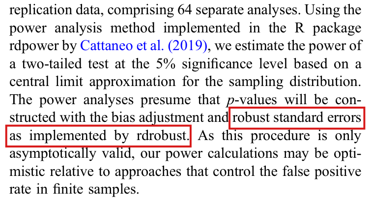
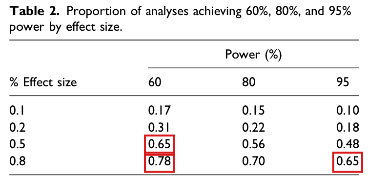
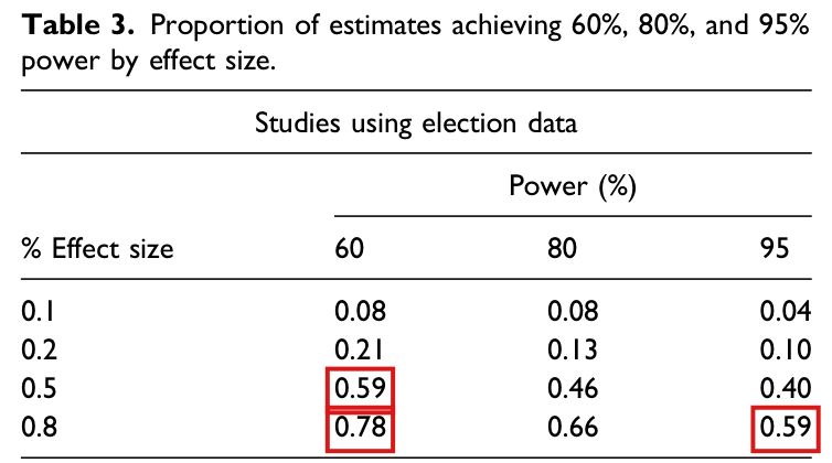
For four clustered estimates, the saved powers match a calculation with a standard error smaller than the robust standard error of rdrobust; with the robust standard error, six cells of Tables 2 and 3 fall by 0.020.02 to 0.040.04.

Power analysis, p. 9 (PDF p. 9), left column; Table 2, p. 9; Table 3, p. 10 (PDF p. 10), panel “Studies using election data”

See also under Formal statements (Lean): P033-T9, P033-T17

As printed

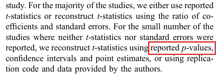
p. 9: “The power analyses presume that pp-values will be constructed with the bias adjustment and robust standard errors as implemented by rdrobust.”

Table 2, p. 9, rows 0.5 and 0.8, as printed.
% Effect size608095
0.50.650.560.48
0.80.780.700.65
Table 3, p. 10, studies using election data, rows 0.5 and 0.8, as printed.
% Effect size608095
0.50.590.460.40
0.80.780.660.59
The problem

The paper says that the power calculation uses the robust standard error of rdrobust. For four sharp clustered estimates, from Gerber and Hopkins (2011), Hall and Thompson (2018), Lopes da Fonseca (2017) and Sances (2017), the saved power does not match this description. Let ss be the robust standard error of the rdrobust fit. Let GG be the number of distinct clusters, and let GLG_L and GRG_R be the numbers of clusters with observations to the left and to the right of the cutoff. All counts are taken after incomplete observations are removed. Each saved power equals the power under the normal approximation with the standard error

s G/(GL+GR)s\,\sqrt{G/(G_L+G_R)}

in place of ss. If there exists a cluster with observations on both sides of the cutoff, I have G<GL+GRG<G_L+G_R. The standard error used for power is then smaller than ss, and the power is too large. Two of the four estimates cross a threshold of the tables. Each has weight 11, and each crossing lowers a cell of Table 2 by 1/361/36 and a cell of the election panel of Table 3 by 1/261/26.

Evidence a recalculation from the source

The evidence is a recalculation from the replication files. Under the normal approximation of p. 9, the test statistic has distribution N(τ/s,1)N(\tau/s,1) when the effect is τ\tau. With a=∣τ∣/sa=|\tau|/s and z=z.975z=z_{.975}, the power of the two-sided 5% test is

f(a)=Φ(a−z)+Φ(−a−z),τ=d σ0,f(a)=\Phi(a-z)+\Phi(-a-z),\qquad \tau=d\,\sigma_0,

where σ0\sigma_0 is the standard deviation of the outcome among control units within the bandwidth. For a>0a>0, I have f′(a)=φ(a−z)−φ(a+z)>0f'(a)=\varphi(a-z)-\varphi(a+z)>0, which implies that the power is strictly larger for a smaller standard error. I had the data of 45 of the 64 estimates. Fitting rdrobust again for these 45 reproduces the saved coefficients and standard errors to a relative error of 4.3×10−154.3\times10^{-15}. The 180 saved powers of these estimates equal f(∣τ∣/(sρ))f(|\tau|/(s\sqrt{\rho})) to within 7×10−167\times10^{-16}, where ρ=1\rho=1 without clusters and ρ=G/(GL+GR)\rho=G/(G_L+G_R) with clusters.

The four estimates: cluster counts and the ratio of the squared standard error used for power to s2s^2.
EstimateGGGLG_LGRG_RG/(GL+GR)G/(G_L+G_R)
Gerber and Hopkins (2011)57234619/2319/23
Hall and Thompson (2018)18598101185/199185/199
Lopes da Fonseca (2017)278202226139/214139/214
Sances (2017)204133130204/263204/263
The three threshold crossings: saved power and the power f(τ/s)f(\tau/s) with the robust standard error.
Estimate and effect sizeSavedWith ssThreshold crossed
Lopes da Fonseca (2017), d=0.5d=0.50.7740.7740.5890.5890.600.60
Lopes da Fonseca (2017), d=0.8d=0.80.9910.9910.9380.9380.950.95
Sances (2017), d=0.8d=0.80.6630.6630.5540.5540.600.60

The powers of Gerber and Hopkins and of Hall and Thompson are also too large, by at most 0.040.04, and cross no threshold. The largest reduction among the four estimates is 0.1850.185. As exact fractions, the Table 2 cells change from 31/4831/48 to 89/14489/144, from 113/144113/144 to 109/144109/144 and from 31/4831/48 to 89/14489/144, and the Table 3 cells from 61/10461/104 to 57/10457/104, from 81/10481/104 to 77/10477/104 and from 61/10461/104 to 57/10457/104. All 36 printed cells are reproduced from the saved powers before the change.

Two limits apply. The source of the rdpower package was not available, and I do not say which of its lines produce the factor. The data files of seven further clustered estimates, from Bohlken (2018), Gulzar and Pasquale (2017) and Larreguy et al. (2016), belong to the replication files, but I did not have them. Their powers were not recomputed, and further cells may change. Note that the estimate of Broockman and Ryan (2016) also has clusters on both sides (G=380G=380, GL=379G_L=379, GR=380G_R=380), but its powers round to 11 with either standard error. Its standard error is the subject of P033-N011.
What survives

Coefficients, standard errors, pp-values, tt-statistics, the caliper tests and the funnel plots do not use the saved powers. The other 30 cells are unchanged by this correction, including the 80% column, so that the percentages quoted in the text (22%, 56% and 70%) stand. The correction lowers power and reinforces the conclusion that the studies are underpowered. It restores the standard error that the paper describes. It does not show that this standard error is right for every clustered design.

Corrected

The sentence of p. 9 stands as the description of the calculation. For the four estimates, the power at effect size dd is

Φ(d σ0/s−z.975)+Φ(−d σ0/s−z.975),\Phi\bigl(d\,\sigma_0/s-z_{.975}\bigr)+\Phi\bigl(-d\,\sigma_0/s-z_{.975}\bigr),

where ss is the robust standard error of the rdrobust fit and σ0\sigma_0 is the standard deviation of the outcome among control units within the default bandwidth. The bandwidths, the effect sizes and the study weights are as in the paper, and all other saved powers are held fixed. This is a partial correction: the seven further clustered estimates are not recomputed.

Table 2, rows 0.5 and 0.8, corrected for the four estimates.
Effect size608095
0.50.620.560.48
0.80.760.700.62
Table 3, studies using election data, rows 0.5 and 0.8, corrected for the four estimates.
Effect size608095
0.50.550.460.40
0.80.740.660.55
Crop of the paragraph that describes the power analysis. A red outline marks the words 'robust standard errors as implemented by rdrobust', which run over two lines.
Power analysis, p. 9 (PDF p. 9), left column. The marked words name the standard error that the power calculation is said to use.
Crop of Table 2, the proportion of analyses achieving 60, 80 and 95 percent power by effect size. Red outlines mark the cells 0.65 (effect size 0.5, power 60), 0.78 (effect size 0.8, power 60) and 0.65 (effect size 0.8, power 95).
Table 2, p. 9 (PDF p. 9). The marked cells are the three that change.
Crop of the first panel of Table 3, 'Studies using election data'. Red outlines mark the cells 0.59 (effect size 0.5, power 60), 0.78 (effect size 0.8, power 60) and 0.59 (effect size 0.8, power 95).
Table 3, p. 10 (PDF p. 10), panel “Studies using election data”. The marked cells are the three that change.

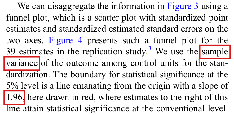
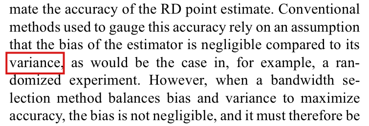
Figure 4 is standardized by the sample standard deviation of the outcome among control units, and its significance boundary has slope 1/z.975≈0.511/z_{.975}\approx0.51, not 1.961.96.

Results, p. 7 (PDF p. 7), right column, paragraph introducing Figure 4

See also under Formal statements (Lean): P033-T10, P033-T11, P033-T18

As printed

We use the sample variance of the outcome among control units for the standardization. The boundary for statistical significance at the 5% level is a line emanating from the origin with a slope of 1.96, here drawn in red, where estimates to the right of this line attain statistical significance at the conventional level.

The problem

The paragraph misstates two features of Figure 4. The figure and the code that draws it are right. First, the estimates and their standard errors are divided by the sample standard deviation of the outcome among observations below the cutoff, not by the sample variance. Second, the figure has the standardized estimate on the horizontal axis and the standardized standard error on the vertical axis. On these axes the line ∣t∣=1.96|t|=1.96 has slope 1/1.961/1.96, the reciprocal of the printed value. A line of slope 1.961.96, with the rule that estimates to its right are significant, would classify estimates with ∣t∣<1.96|t|<1.96 as significant.

Evidence a historical Lean attribution (Generated status: clause support not certified in this release)

The evidence is a derivation, an exact counterexample to the printed slope, and a check of the code and of one study in the replication files. Let s0>0s_0>0 be the sample standard deviation of the outcome among control units, τ^\widehat\tau an estimate and SE^>0\widehat{\mathrm{SE}}>0 its standard error. The figure plots

x=∣τ^∣/s0,y=SE^/s0,x=|\widehat\tau|/s_0,\qquad y=\widehat{\mathrm{SE}}/s_0,

so that x/y=∣τ^∣/SE^=∣t∣x/y=|\widehat\tau|/\widehat{\mathrm{SE}}=|t|. Let z=z.975z=z_{.975}. Since y>0y>0 and z>0z>0, I have ∣t∣≥z|t|\ge z if and only if y≤x/zy\le x/z. The boundary is the line y=x/zy=x/z through the origin, with slope 1/z≈0.51021/z\approx0.5102, and the significant estimates lie to its right.

For the counterexample, let z=1.96=49/25z=1.96=49/25. The point (x,y)=(1/2,1/2)(x,y)=(1/2,1/2) has ∣t∣=1<1.96|t|=1<1.96. At height y=1/2y=1/2 the line of slope 49/2549/25 passes through x=25/98<1/2x=25/98<1/2. The point lies to the right of that line and is not significant.

The plotting script of the replication files draws the line with slope 1/qnorm(0.975) and divides both coordinates by y0_sd. The analysis script computes this divisor with sd() over the observations below the cutoff. For Boas and Hidalgo (2011), these are 568 observations with 82 ones and 486 zeros. Their sample variance is 123/994≈0.124123/994\approx0.124, and the saved divisor agrees with 123/994≈0.3518\sqrt{123/994}\approx0.3518. I checked this one study only.

What survives

Figure 4, its red line, the estimates, the standard errors and every classification as significant are unchanged. The power analysis uses its own standard deviation, that of control units within the default bandwidth (p. 9), which this correction does not touch. Only the two terms in the description change.

Corrected

We use the sample standard deviation of the outcome among control units for the standardization. The boundary for statistical significance at the 5% level is a line emanating from the origin with a slope of 1/z.975≈1/1.961/z_{.975}\approx1/1.96, here drawn in red, where estimates to the right of this line attain statistical significance at the conventional level.

Here the horizontal axis is the absolute standardized estimate ∣τ^∣/s0|\widehat\tau|/s_0 and the vertical axis is its standardized standard error SE^/s0\widehat{\mathrm{SE}}/s_0, as in the published figure.

Crop of the paragraph that introduces the funnel plot. Red outlines mark the word 'sample' at the end of one line, the word 'variance' at the start of the next, and the number '1.96' in the sentence about the slope of the significance boundary.
Results, p. 7 (PDF p. 7), right column. The marked terms are “sample variance”, broken across two lines, and the slope “1.96”.

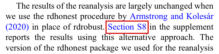
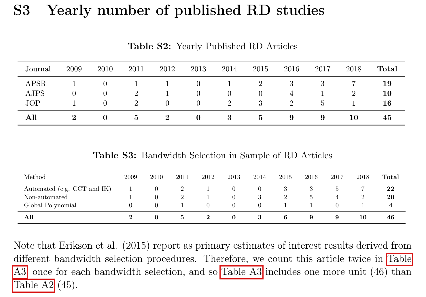
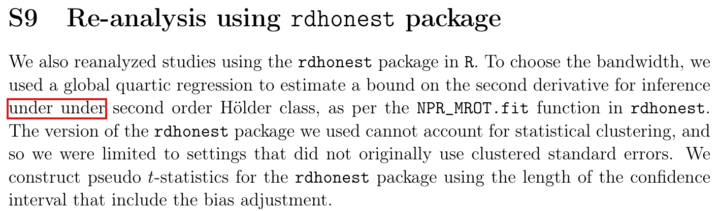
The rdhonest results are in Section S9 of the supplement, not Section S8, and the note below Table S3 calls Tables S3 and S2 “Table A3” and “Table A2”.

p. 8 (PDF p. 8), left column, paragraph on the rdhonest procedure; online supplement, p. 8, note below Table S3

As printed

Main text, p. 8: “Section S8 in the supplement reports the results using this alternative approach.”

Supplement, p. 8: “Therefore, we count this article twice in Table A3, once for each bandwidth selection, and so Table A3 includes one more unit (46) than Table A2 (45).”

The problem

Two cross-references point to the wrong place. Section S8 of the supplement is “All studies with replication data”. The results of the rdhonest reanalysis are in Section S9, “Re-analysis using rdhonest package”. The reference to Section S8 on p. 7, for the reanalysis of all 36 studies, is right. The supplement has no Table A2 or A3. The note stands below Tables S2 and S3 and explains their totals, 45 and 46.

Evidence a check of the printed page

The evidence is a check of the page for the main text. For the supplement I had the text of the official file and the page image shown above, not the PDF itself. The headings of Sections S8 and S9 and the titles and totals of Tables S2 and S3 are as stated. The table files of the replication files carry the same two tables.

What survives

Correcting these labels changes no number or result.

Corrected

Main text, p. 8: “Section S9 in the supplement reports the results using this alternative approach.”

Supplement, p. 8: “Therefore, we count this article twice in Table S3, once for each bandwidth selection, and so Table S3 includes one more unit (46) than Table S2 (45).”

Crop of the paragraph that begins 'The results of the reanalysis are largely unchanged'. A red outline marks the words 'Section S8' in its second sentence.
p. 8 (PDF p. 8), left column. The marked reference is “Section S8”.
Crop of a supplement page with the heading 'S3 Yearly number of published RD studies', Table S2 with total 45, Table S3 with total 46, and a four-line note. Red outlines mark 'Table' at the end of one line with 'A3' at the start of the next, then 'Table A3', then 'Table A2'.
Online supplement, p. 8: Tables S2 and S3 and the note below them. The marked labels are “Table A3” (twice) and “Table A2”.

Tables S2 and S3 count the study of Schickler, Pearson and Feinstein in 2009, but it was published in 2010, and the 2009 and 2010 entries of four rows are each off by one.

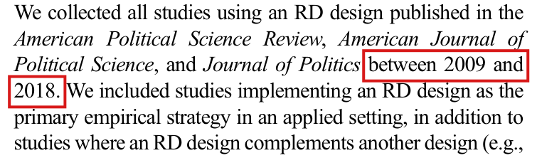
Supplement, Section S3, Tables S2 and S3, p. 8; the sample period is stated on p. 4 (PDF p. 4) of the main text, right column

As printed

Main text, p. 4: “We collected all studies using an RD design published in the American Political Science Review, American Journal of Political Science, and Journal of Politics between 2009 and 2018.”

Table S2 (Yearly Published RD Articles) and Table S3 (Bandwidth Selection in Sample of RD Articles), Supplement p. 8: the columns 2009, 2010 and Total, as printed. The columns 2011 to 2018 are not affected.
TableRow20092010Total
S2APSR1019
S2AJPS0010
S2JOP1016
S2All2045
S3Automated (e.g. CCT and IK)1022
S3Non-automated1020
S3Global Polynomial004
S3All2046
The problem

The two tables count Schickler, Pearson and Feinstein in 2009. Table S1 and the reference list of the supplement cite the study as 2010, in The Journal of Politics 72(3), 672–689. According to the publisher, the article appeared online on 12 July 2010 and in the print issue of July 2010, and no date in 2009 is listed. The study therefore belongs in 2010 whether an article is dated by its first online publication or by its issue. In the replication code the year is read from the internal label of the article, schickler_etal_2009. The study is in the JOP row of Table S2, the Non-automated row of Table S3 and both All rows. In each of these four rows the 2009 entry is one too high and the 2010 entry is one too low.

A second study is counted in a year other than its cited year. Cavaillé and Marshall is cited as 2019, in American Political Science Review 113(1), and is counted among the seven APSR articles of 2018. It appeared online on 15 November 2018 and in the issue of February 2019. Its count in 2018, and its place in the period 2009–2018, are correct if articles are dated by first online publication. The paper does not state this rule.

Evidence a recalculation from the source

This correction rests on a recalculation from the replication files and on the publisher’s dates. When the table code is run unchanged, it reproduces Tables S2 and S3. When only the year of this study is changed to 2010, the eight highlighted entries change and no others, and Tables 2, 3 and S6, which the same script produces, do not change. The entries of Tables S2 and S3 are taken from the extracted text of the supplement and from the tables in the replication files, which agree; I did not have the typeset supplement pages.

What survives

All row totals, the sample of 45 studies, and every estimate and weight are unchanged, since no analysis uses the year of publication. Only the eight annual counts change.

Corrected
Tables S2 and S3: the columns 2009, 2010 and Total, corrected. The columns 2011 to 2018 are as printed.
TableRow20092010Total
S2APSR1019
S2AJPS0010
S2JOP0116
S2All1145
S3Automated (e.g. CCT and IK)1022
S3Non-automated0120
S3Global Polynomial004
S3All1146

If Cavaillé and Marshall is retained in 2018, Section S3 should state the dating rule: Articles are counted in the year of their first online publication. Under this rule Cavaillé and Marshall (2019) is counted in 2018.

Crop of six lines of the right column of page 4. Red boxes mark the words 'between 2009 and' at the end of one line and '2018.' at the start of the next, in the sentence 'We collected all studies using an RD design published in the American Political Science Review, American Journal of Political Science, and Journal of Politics between 2009 and 2018.'
Section “The state of RD studies in political science”, first sentence, p. 4 (PDF p. 4), right column. The marked words give the sample period, without saying how an article is dated.
Crop of one entry of the reference list of the supplement: 'Schickler, E., Pearson, K., and Feinstein, B. D. (2010). Congressional parties and civil rights politics from 1933 to 1972. The Journal of Politics, 72(3), 672-689.' A red box marks the year '(2010)'.
Supplement, reference list, p. 23. The supplement itself cites the study with the marked year 2010.

“worse-case” should read “worst-case”, “insofar as it as possible” should read “insofar as it is possible”, “This is section” should read “In this section”, “the manually feed” should read “then manually feed”, and one “under” in “under under” should be deleted.

p. 4 (PDF p. 4), left column; p. 11 (PDF p. 11), left column; Supplement, Section S6, p. 12, and Section S9, p. 16

As printed
  • p. 4: “The third approach is to adjust the inference procedure with the worse-case bias consistent with the observed data.”
  • p. 11: “However, insofar as it as possible, having a full record of analyses that were intended would be helpful for the accumulation of knowledge.”
  • Supplement, p. 12: “This is section we document all failures to reproduce the authors' original estimates during our replication.”
  • Supplement, p. 12: “When reproducing their estimates we select the bandwidth through the rdbwselect_2014 for backward compatibility purposes, and the manually feed this bandwidth into the rdrobust package.”
  • Supplement, p. 16: “… to estimate a bound on the second derivative for inference under under second order Hölder class …”
The problem

Each of the five phrases has a wrong, missing or repeated word. The meaning is clear in every case.

Evidence a check of the printed page

I checked the pages for the two phrases of the main text. The sentence after the first one prints “The worst-case is taken with respect to a stipulated class of functions”, and p. 8 prints “worst-case bias adjustment”. I compared the three supplement phrases in its extracted text with the marked images of those passages accompanying this entry; they agree. I did not have the typeset supplement pages for comparison.

What survives

Everything else is unaffected, since no statement of the paper depends on these words.

Corrected
  • p. 4: “The third approach is to adjust the inference procedure with the worst-case bias consistent with the observed data.”
  • p. 11: “However, insofar as it is possible, having a full record of analyses that were intended would be helpful for the accumulation of knowledge.”
  • Supplement, p. 12: “In this section we document all failures to reproduce the authors' original estimates during our replication.”
  • Supplement, p. 12: “… and then manually feed this bandwidth into the rdrobust package.”
  • Supplement, p. 16: “… for inference under second order Hölder class …”
Crop of four lines of the left column of page 4. A red box marks the word 'worse-case' in 'with the worse-case bias consistent with the observed data'. The next sentence begins 'The worst-case is taken with respect to a stipulated class of functions'.
Paragraph beginning “The third approach”, p. 4 (PDF p. 4), left column. The marked word should read “worst-case”, as in the next sentence.
Crop of five lines of the left column of page 11. A red box marks the words 'it as possible,' in the sentence 'However, insofar as it as possible, having a full record of analyses that were intended would be helpful for the accumulation of knowledge.'
Paragraph on preregistration, p. 11 (PDF p. 11), left column. The marked words should read “it is possible”.
Crop of the heading 'S6 Reproduction of originally reported estimates' and the two paragraphs under it. Red boxes mark the words 'This is section' at the start of the first paragraph and the words 'the manually feed' in the entry for de Benedictis-Kessner and Warshaw (2016).
Supplement, Section S6, p. 12. The first marked phrase should read “In this section” and the second “then manually feed”.
Crop of the heading 'S9 Re-analysis using rdhonest package' and the paragraph under it. A red box marks the words 'under under' at the start of the third line, before 'second order Hölder class'.
Supplement, Section S9, p. 16, first paragraph. The marked word is printed twice.

The first column of Tables 2 and 3 gives effect sizes in units of Cohen’s dd, and the percent sign in its heading does not belong there.

Table 2, p. 9 (PDF p. 9), and both panels of Table 3, p. 10 (PDF p. 10): heading of the first column

As printed

First-column heading of Table 2 and of both panels of Table 3: “% Effect size”, above the rows 0.1, 0.2, 0.5 and 0.8.

The problem

The rows of the first column are the four values of Cohen’s dd defined on p. 9, in units of the standard deviation of the outcome. They are not percentages. The percent sign belongs only to the columns, which are the power thresholds 60, 80 and 95 under the heading “Power (%)”. No entry of the tables needs rescaling.

Evidence a check of the printed page

The evidence is a check of the pages and of the replication files. The table files there carry the heading “Effect size”. The analysis script multiplies each value of dd by the standard deviation of the outcome and does not convert it to a percentage.

What survives

All entries of the tables, the power calculations and the comparisons drawn from them are unchanged.

Corrected

“Effect size (Cohen’s dd)”, without the percent sign, in Table 2 and in both panels of Table 3. Deleting the percent sign alone is also correct.

Crop of Table 2. A red outline marks the percent sign that precedes the words 'Effect size' in the heading of the first column.
Table 2, p. 9 (PDF p. 9). The marked character is the percent sign in the heading of the first column.
Crop of Table 3 with its two panels, 'Studies using election data' and 'Studies not using election data'. In each panel a red outline marks the percent sign that precedes the words 'Effect size'.
Table 3, p. 10 (PDF p. 10), both panels. The marked characters are the percent signs in the two headings of the first column.

The histograms of Figures 1, 2, 3 and 5 leave out every tt-statistic above 3.923.92 and scale each density to the weight that remains, and each panel of Figure 4 leaves out 3 or 4 of the 39 estimates; the text and the captions do not say so.

p. 4 (PDF p. 4), right column, paragraph beginning “Figure 1 presents the distribution”; p. 7 (PDF p. 7); Figures 1, 2, 3, 4 and 5 (pp. 5, 6, 8 and 10)

As printed

p. 4: “Figure 1 presents the distribution of tt-statistics for the published findings among all 45 studies in our sample. The first panel presents the distribution of the main reported result of each article, meaning that each article contributes one tt-statistic.”

p. 7: “Figure 3 presents the distribution of tt-statistics among the 39 estimates from the 25 studies included in the main replication exercise.”

p. 7: “Figure 4 presents such a funnel plot for the 39 estimates in the replication study.”

Vertical axis of panels (a) of Figures 1, 2 and 3: “Density”.

The problem

The code for the histograms sets the horizontal axis to the interval from 00 to 2Φ−1(0.975)2\Phi^{-1}(0.975), which is approximately [0,3.92][0,3.92]. A tt-statistic above this limit enters no bin, and the density of each panel is then normalized to the weight that remains in the interval. Figure 1(a) shows 37 of the 45 main results, and each of its bars is higher by the factor 45/3745/37 than it would be in a density of all 45. Let WW be the total weight of the sample named in the text, let VV be the weight in the interval, and let BjB_j be the weight in bin jj, where each bin has width w=Φ−1(0.975)/18w=\Phi^{-1}(0.975)/18. The printed height of bin jj is Bj/(wV)B_j/(wV), and the height in a density of the full sample is Bj/(wW)B_j/(wW). The printed heights are those of the distribution conditional on t≤2Φ−1(0.975)t\le 2\Phi^{-1}(0.975).

The share of weight left out differs across panels. In Figure 3 it is 21%, 26% and 29% in panels (a), (b) and (c). The three panels that the text compares are conditioned on different sets. The funnel plots of Figure 4 have axis limits 0≤x≤20\le x\le 2 and 0≤y≤0.80\le y\le 0.8, and panels (a), (b) and (c) leave out 3, 3 and 4 of the 39 estimates. The main text, the captions and the text of the supplement state neither the omissions nor the normalization. The range of each axis is visible in the figures, and the counts 45, 80 and 39 given in the text are the correct sizes of the samples that enter the code.

Evidence a recalculation from the source

This correction rests on a recalculation from the replication files and on a measurement of the published figure. The table lists what each panel leaves out, computed from the stored tt-statistics and the weights of the paper.

Histogram panels: statistics that enter the code, statistics above the axis limit, share of weight left out, and the factor W/VW/V by which the printed bars exceed a density of the full sample.
PanelStatisticsLeft outShare of weight left outW/VW/V
1(a)4588/45=17.8%8/45=17.8\%45/37=1.21645/37=1.216
1(b)801229/180=16.1%29/180=16.1\%180/151=1.192180/151=1.192
2(a)4243/22=13.6%3/22=13.6\%22/19=1.15822/19=1.158
2(b)38817/92=18.5%17/92=18.5\%92/75=1.22792/75=1.227
3(a)39921/100=21.0%21/100=21.0\%100/79=1.266100/79=1.266
3(b)391013/50=26.0%13/50=26.0\%50/37=1.35150/37=1.351
3(c)391029/100=29.0%29/100=29.0\%100/71=1.408100/71=1.408
5(a)47717/124=13.7%17/124=13.7\%124/107=1.159124/107=1.159
5(b)3353/14=21.4%3/14=21.4\%14/11=1.27314/11=1.273

The bars of Figure 1(a) in the published PDF represent 37 results in total. A bar that holds one result has measured height 0.24820.2482. This agrees with 1/(37w)=0.24821/(37w)=0.2482 and not with 1/(45w)=0.20411/(45w)=0.2041. The figures in the replication files contain 36, 36 and 35 points for the three panels of Figure 4.

What survives

Within a panel, the order of the bars, the position of the spike near 1.961.96 and the ratios between bars are unchanged, since every bar of the panel is rescaled by the same constant. Table 1 and Tables S4 and S5 use their designated main-estimate samples without these plotting limits, and their windows end below the axis limit. Tables 2 and 3 use all 64 analyses. In the full data the weighted share of tt-statistics at or above 1.961.96 is 0.770.77, 0.630.63 and 0.490.49 for the samples of Figure 3(a), (b) and (c), so this decline in the share of significant results holds without the axis limit. The absolute scale of the densities and comparisons of bar heights between panels do change.

Corrected

The following note should accompany Figures 1, 2, 3 and 5. Each histogram shows the tt-statistics in the interval from 00 to 2Φ−1(0.975)2\Phi^{-1}(0.975), approximately [0,3.92][0,3.92]. The density is normalized to the weight in that interval, separately in each panel. The panels leave out 8 of 45, 12 of 80, 4 of 42, 8 of 38, 9 of 39, 10 of 39, 10 of 39, 7 of 47 and 5 of 33 statistics in Figures 1(a), 1(b), 2(a), 2(b), 3(a), 3(b), 3(c), 5(a) and 5(b), which is 17.8%, 16.1%, 13.6%, 18.5%, 21.0%, 26.0%, 29.0%, 13.7% and 21.4% of the weight.

The following note should accompany Figure 4. The panels show the estimates within the axis limits. Panels (a), (b) and (c) leave out 3, 3 and 4 of the 39 estimates.

If the heights are instead to describe the full sample, each printed bar is multiplied by V/WV/W, the reciprocal of the factor in the table above, and the weight outside the interval is reported.

Crop of five lines of the right column of page 4. A red box marks the words 'among all 45 studies in our sample.' in the sentence 'Figure 1 presents the distribution of t-statistics for the published findings among all 45 studies in our sample.'
Paragraph beginning “Figure 1 presents the distribution”, p. 4 (PDF p. 4), right column. The marked words give the sample that the figure is said to show.
Crop of Figure 1 with its caption: two histograms of t-statistics, panel (a) 'Main reported result' and panel (b) 'All primary results', each with a vertical line at 1.96, a horizontal axis with ticks at 0.98, 1.96, 2.94 and 3.92, and a vertical axis from 0 to 2. Red boxes mark the vertical-axis label 'Density' of panel (a) and the tick label '3.92' at the right end of its horizontal axis.
Figure 1, p. 5 (PDF p. 5). The marked labels of panel (a) are the vertical axis, “Density”, and the last tick of the horizontal axis, 3.923.92. The panel shows 37 of the 45 main results.

The replication code reconstructs no tt-statistic from a reported pp-value, and it computes a standard error from a confidence interval as the full width divided by twice the critical value, not from the upper limit and the point estimate as Section S4 says.

p. 4 (PDF p. 4), right column, last sentence of the paragraph beginning “Figure 1 presents the distribution”; Supplement, Section S4, pp. 9–10

See also under Formal statements (Lean): P033-T14, P033-T15

As printed

Main text, p. 4: “For the small number of the studies where neither tt-statistics nor standard errors were reported, we reconstruct tt-statistics using reported pp-values, confidence intervals and point estimates, or using replication code and data provided by the authors.”

Supplement, Section S4, entry for Ariga (2015): “The standard error estimate was imputed by (a) subtracting the point estimate value from the upper value of the reported 90% confidence interval, and then (b) dividing that value by the critical value for a 90% confidence interval (1.64).”

Supplement, Section S4, entries for Holbein (2016) and for Kalšnja and Titiunik (2017), as named in the extracted text: “The standard error was not explicitly listed and so we imputed by using the upper bound of a 95% CI and the point estimate along with the critical value of 1.96.”

The problem

The description of how missing tt-statistics were reconstructed differs from the replication code in two respects. First, the code fills a missing standard error from a reported tt-statistic, from a 90% or 95% confidence interval, or from the replication data, and then computes every missing tt-statistic as the absolute estimate divided by the standard error. No tt-statistic is recovered from a reported pp-value. Second, for a reported interval [L,U][L,U] and point estimate bb, the code computes the standard error as (U−L)/(2q)(U-L)/(2q), where qq is Φ−1(0.95)\Phi^{-1}(0.95) for a 90% interval and Φ−1(0.975)\Phi^{-1}(0.975) for a 95% interval. Section S4 instead describes the rule (U−b)/q(U-b)/q for Ariga, for Holbein, and for Klašnja and Titiunik. The two rules agree only when the interval is centered on the estimate. Of the six estimates to which Section S4 applies this rule, four have a recorded interval that is not exactly centered. For three of them the two standard errors differ by less than 1%, and for Klašnja and Titiunik they differ by the factor 8/78/7.

Evidence an exact counterexample

This correction rests on a derivation, an exact example and a recalculation from the replication files. I checked the Supplement Section S4 quotations against its extracted text; I did not have the typeset supplement pages. Set sW=(U−L)/(2q)s_W=(U-L)/(2q) and sU=(U−b)/qs_U=(U-b)/q. Then

2q (sW−sU)=(U−L)−2(U−b)=2b−U−L,2q\,(s_W-s_U)=(U-L)-2(U-b)=2b-U-L,

which implies that sW=sUs_W=s_U if and only if b=(U+L)/2b=(U+L)/2. For Klašnja and Titiunik the recorded values are b=−0.15b=-0.15 and [L,U]=[−0.213,−0.101][L,U]=[-0.213,-0.101]. Then U−L=0.112U-L=0.112 and U−b=0.049U-b=0.049, and I obtain sW/sU=8/7s_W/s_U=8/7 for every q>0q>0. At the printed critical value q=1.96q=1.96, I have sW=1/35s_W=1/35 and sU=1/40s_U=1/40, and the absolute tt-statistics are 21/4=5.2521/4=5.25 and 66. The replication code, which uses q=Φ−1(0.975)q=\Phi^{-1}(0.975), gives 5.24995.2499.

Of the 81 rows of the raw metadata, 65 report a standard error, 1 reports a tt-statistic, 2 use a 90% interval, 10 use a 95% interval and 3 use replication data. After every reported pp-value is erased from the raw metadata, the cleaning code returns the same 81 standard errors and tt-statistics.

What survives

Correcting the description changes no numerical result, and the cleaning code reproduces the cleaned data exactly. The reanalysis, its caliper tests and the power calculations do not use the imputed standard errors. If the rule of Section S4 were applied instead, with its printed critical values, Tables 1 and S4 would keep their counts and pp-values. One estimate of Holbein (2016) would move by one histogram bin in Figures 1(b), 2(b) and 5(b), and six entries of Table S6 would change.

Corrected

Main text, p. 4: “For the small number of the studies where neither tt-statistics nor standard errors were reported, we reconstruct tt-statistics using reported pp-values, confidence intervals and point estimates, or using replication code and data provided by the authors.”

Supplement, Section S4, entry for Ariga (2015): the standard error is the width U−LU-L of the reported 90% confidence interval [L,U][L,U] divided by 2Φ−1(0.95)2\Phi^{-1}(0.95).

Supplement, Section S4, entries for Holbein (2016) and for Klašnja and Titiunik (2017): the standard error is the width U−LU-L of the reported 95% confidence interval [L,U][L,U] divided by 2Φ−1(0.975)2\Phi^{-1}(0.975).

In each case the tt-statistic is the absolute point estimate divided by this standard error. Reported pp-values are recorded separately, and a missing pp-value is derived from the tt-statistic by the normal approximation.

Crop of seven lines of the right column of page 4. A red box marks the words 'reported p-values,' in the sentence 'For the small number of the studies where neither t-statistics nor standard errors were reported, we reconstruct t-statistics using reported p-values, confidence intervals and point estimates, or using replication code and data provided by the authors.'
End of the paragraph on Figure 1, p. 4 (PDF p. 4), right column. The marked words name a source that the replication code does not use to reconstruct a tt-statistic.

The pp-values of Table 1 are binomial tails under equal probability mass on the two sides of 1.961.96 within each window, and this condition does not follow from the absence of selection on significance alone.

p. 5 (PDF p. 5), left column, paragraph beginning “Table 1 presents the results from the caliper tests”, and Table 1

See also under Formal statements (Lean): P033-T7, P033-T8

As printed

We calculate the probability of observing an imbalance at least this extreme under the null hypothesis of no real pathologies in the RD literature by using a binomial distribution with equal success probability, capturing that we would expect a study to be equally likely to be just above and below the threshold under the null. […] The pp-values of the caliper tests range between 3% and 7%, depending on the window size, indicating that it is unlikely that we would observe this large of an imbalance in the tt-statistics if there were no real pathologies in the RD literature.

The problem

The counts of Table 1 and its binomial tail probabilities are correct. The calculation takes each study in a window to lie above 1.961.96 with probability 1/21/2. Let ff be the density of the absolute tt-statistic when publication does not depend on significance, set c=1.96c=1.96, and let hh be the half-width of the window. Define

Ah=∫cc+hf(x) dx,Bh=∫c−hcf(x) dx,ph=AhAh+Bh.A_h=\int_c^{c+h}f(x)\,dx,\qquad B_h=\int_{c-h}^{c}f(x)\,dx,\qquad p_h=\frac{A_h}{A_h+B_h}.

A study in the window lies above cc with probability php_h, and ph=1/2p_h=1/2 exactly when Ah=BhA_h=B_h. The null hypothesis that the 5% level plays no part in publication does not imply this equality at the half-widths 0.1960.196, 0.2940.294 and 0.3920.392 that the paper uses. If ff is differentiable at cc and f(c)>0f(c)>0, then

ph−12=h f′(c)4f(c)+o(h),p_h-\frac12=\frac{h\,f'(c)}{4f(c)}+o(h),

which shows that the two counts are approximately equal as hh tends to zero, as the preceding paragraph of the paper says. No bound follows at a fixed hh. The passage reads the tails of 3% to 7% as the probability of the imbalance when there is no selection, and that reading requires the further condition Ah=BhA_h=B_h, at least approximately. Equal mass on the two sides is the usual working assumption of the caliper test, which the paper takes from Gerber and Malhotra (2008a, 2008b).

Evidence an exact counterexample

This correction rests on exact counterexamples. Suppose that the studies are independent, that every study is published, and that the absolute tt-statistic has density f(x)=x/8f(x)=x/8 on [0,4][0,4]. This density is smooth and positive on every window and has no jump at 1.961.96. With c=49/25c=49/25, a direct computation gives Ah=(2ch+h2)/16A_h=(2ch+h^2)/16 and Bh=(2ch−h2)/16B_h=(2ch-h^2)/16, so that ph=1/2+h/(4c)p_h=1/2+h/(4c). For h=c/10h=c/10, 3c/203c/20 and c/5c/5, I obtain ph=21/40p_h=21/40, 43/8043/80 and 11/2011/20. Given nn studies in the window, the number above cc is binomial with parameters nn and php_h. The table compares the upper tails at the counts of Table 1.

One-sided binomial tails at the counts of Table 1: with probability 1/21/2, as printed, and with the probability php_h of the density f(x)=x/8f(x)=x/8.
WindowBelowAboveTail with 1/21/2Tail with php_h
10%39299/4096=0.073299/4096=0.0730.1000.100
15%4111941/32768=0.0591941/32768=0.0590.1020.102
20%5142083/65536=0.0322083/65536=0.0320.0780.078

With 19 studies in the 20% window, the test at the 5% level rejects exactly when at least 14 lie above cc, and under this density it rejects with probability 0.07770.0777. In a second example each study has an unbiased normal estimate with standard error 11 and true effect 7/27/2, and every study is published. In the 20% window, php_h then lies between 0.6447477581040.644747758104 and 0.6447477581050.644747758105, and the tail at 14 of 19 lies between 0.2804134616770.280413461677 and 0.2804134616780.280413461678. If instead every true effect is zero, then php_h is approximately 0.31890.3189 and the one-sided test is conservative. I note that these examples are not estimates of php_h for the 45 studies of the paper. For those studies I have established neither the size of the error nor its direction.

What survives

The counts, the imbalance of about three to one and the histograms are unchanged, and so are the entries of Table 1 when they are read as tails under equal mass on the two sides. The reanalysis and the power calculations do not use these probabilities. The reading of the 3% to 7% as the probability of the imbalance in the absence of selection does change. It now requires equal mass on the two sides, and the same holds for Tables S4 and S5 and for the discussion of bandwidth groups on p. 6.

Corrected

The first of the two sentences quoted above is replaced by the following. “Conditional on the number of studies in each caliper, we calculate one-sided binomial tail probabilities under a working null of equal probability mass above and below the threshold. Interpreting these probabilities as evidence of publication bias requires an additional justification that the unselected distribution has approximately equal mass on the two sides, or a sensitivity analysis allowing unequal mass. Publication independence alone does not imply the working null.” The second sentence, on the range of 3% to 7%, is then a statement about this working null.

In full, the statement is as follows. Let c=1.96c=1.96 and let 0<h<c\colorbox{#ffe58a}{$0<h<c$} be the half-width of a window. Suppose that the studies are independent and that, in the absence of selection, the absolute tt-statistic of each study has density ff. Let AhA_h and BhB_h be the integrals of ff over [c,c+h][c,c+h] and [c−h,c][c-h,c], with Ah+Bh>0\colorbox{#ffe58a}{$A_h+B_h>0$}. Conditional on nn studies in the window [c−h,c+h][c-h,c+h], the number KK above cc is binomial with parameters nn and ph=Ah/(Ah+Bh)p_h=A_h/(A_h+B_h), and

Pr⁡(K≥k∣n)=∑j=kn(nj)ph j(1−ph)n−j.\Pr(K\ge k\mid n)=\sum_{j=k}^{n}\binom{n}{j}p_h^{\,j}(1-p_h)^{n-j}.

The entries of Table 1 are the values of this sum at ph=1/2p_h=1/2, which is the case Ah=BhA_h=B_h. If ff is nonincreasing on the window, then ph≤1/2p_h\le 1/2 and the one-sided test is conservative. If f≥m>0f\ge m>0 and ff is LL-Lipschitz on the window, then ∣ph−1/2∣≤Lh/(4m)|p_h-1/2|\le Lh/(4m). Table 1 itself is unchanged.

Crop of nine lines of the left column of page 5. Red boxes mark the words 'null hypothesis of no real pathologies' and, two lines below, 'equal success probability,' in the sentence 'We calculate the probability of observing an imbalance at least this extreme under the null hypothesis of no real pathologies in the RD literature by using a binomial distribution with equal success probability'.
Paragraph beginning “Table 1 presents the results from the caliper tests”, p. 5 (PDF p. 5), left column. The first marked phrase is the null hypothesis that is named, and the second is the probability that the calculation uses.

The third author of Hahn, Todd and Van der Klaauw (2001) is printed as “Klaauw W”, and the entry for Imbens and Kalyanaraman pairs the year 2011 with volume 79(3), which is an issue of 2012.

References, p. 12 (PDF p. 12), entries for Hahn et al. (2001) and Imbens and Kalyanaraman (2011); both are cited on p. 3

As printed

Hahn J, Todd P and Klaauw W (2001) Identification and estimation of treatment effects with a regression-discontinuity design. Econometrica 69(1): 201–209.

Imbens G and Kalyanaraman K (2011) Optimal bandwidth choice for the regression discontinuity estimator. The Review of Economic Studies 79(3): 933–959.

The problem

The surname of the third author is Van der Klaauw, and the entry drops part of it. Volume 79, issue 3 of The Review of Economic Studies is the issue of July 2012. The article appeared online in advance on 24 November 2011. The year 2011 is a date of the article, but it does not match the volume and issue that the entry cites. Both entries still identify the works.

Evidence a check of the printed page

The evidence is a check of the page and of the publishers' pages for the two articles. The byline of the Econometrica article reads “Wilbert Van der Klaauw”. The page of the second article reads “Volume 79, Issue 3, July 2012, Pages 933–959”, with the publication date 24 November 2011.

What survives

No argument or result of the paper depends on either detail.

Corrected

Hahn J, Todd P and Van der Klaauw W (2001) Identification and estimation of treatment effects with a regression-discontinuity design. Econometrica 69(1): 201–209.

Imbens G and Kalyanaraman K (2012) Optimal bandwidth choice for the regression discontinuity estimator. The Review of Economic Studies 79(3): 933–959.

The year 2011 can be kept if the entry says that it is the year of advance online publication. The citation on p. 3 follows the year chosen.

Crop of three entries of the reference list: Hahn, Todd and Klaauw (2001), Hall (2015), and Imbens and Kalyanaraman (2011). Red outlines mark 'Klaauw W' in the first entry and '(2011)' in the third.
References, p. 12 (PDF p. 12), right column. The marked terms are the author name “Klaauw W” and the year “(2011)”.

Clarity notes

Imprecise or ambiguous wording whose intended meaning is correct; not an error.

Conventional inference requires the bias of the estimator to be negligible compared to its standard deviation, not its variance.

Section “Why is it hard to estimate RD effects?”, p. 3 (PDF p. 3), right column, paragraph beginning “The use of bandwidth selection methods to maximize accuracy”

As printed

Conventional methods used to gauge this accuracy rely on an assumption that the bias of the estimator is negligible compared to its variance, as would be the case in, for example, a randomized experiment.

Intended meaning

The sentence means that the standardized bias is negligible, that is, that the bias is small relative to the standard deviation of the estimator. This is the correct condition. I write the estimator as Tn=θ+bn+snZnT_n=\theta+b_n+s_nZ_n, where bnb_n is its bias, sns_n is its standard deviation, and ZnZ_n converges in distribution to N(0,1)N(0,1). With a consistent standard error, conventional inference centered at θ\theta relies on

Tn−θsn=Zn+bnsn\frac{T_n-\theta}{s_n}=Z_n+\frac{b_n}{s_n}

having a standard normal limit, which holds when ∣bn∣/sn→0|b_n|/s_n\to 0, or equivalently bn2/sn2→0b_n^2/s_n^2\to 0.

The ratio of the bias to the variance is a different quantity, and it depends on the units of the outcome, since multiplying the outcome by aa multiplies the bias by aa and the variance by a2a^2. For independent Xi∼N(θ,1)X_i\sim N(\theta,1) and Tn=Xˉn+n−3/4T_n=\bar X_n+n^{-3/4}, I have bn/sn=n−1/4→0b_n/s_n=n^{-1/4}\to 0 and bn/sn2=n1/4→∞b_n/s_n^2=n^{1/4}\to\infty. The conventional 95% interval then has coverage Φ(z0.975−n−1/4)−Φ(−z0.975−n−1/4)\Phi(z_{0.975}-n^{-1/4})-\Phi(-z_{0.975}-n^{-1/4}), which equals 0.9384670.938467 at n=100n=100 and 0.9488540.948854 at n=10,000n=10{,}000, and tends to 0.950.95. No estimator, code or result of the paper uses the printed wording.

Corrected

Conventional methods used to gauge this accuracy rely on an assumption that the bias of the estimator is negligible compared to its standard deviation, as would be the case in, for example, a randomized experiment.

An equivalent wording is that the squared bias of the estimator is negligible compared to its variance.

Crop of seven lines of the right column of page 3. A red box marks the word 'variance' in the sentence 'Conventional methods used to gauge this accuracy rely on an assumption that the bias of the estimator is negligible compared to its variance, as would be the case in, for example, a randomized experiment.'
Section “Why is it hard to estimate RD effects?”, p. 3 (PDF p. 3), right column. The marked word gives the scale against which the bias is compared.

The opening identification argument is the argument for a sharp RD design, and the paragraph does not say “sharp”.

Section “Why is it hard to estimate RD effects?”, first paragraph, p. 3 (PDF p. 3), left column

As printed

The causal effect studied in the RD design is the difference between the expected treated and control potential outcomes at a cutoff where treatment assignment changes in a discontinuous fashion. If the conditional expectation function of the outcome were known, this effect can be calculated without error under an assumption that the conditional expectation functions of the potential outcomes are continuous at the cut point. In other words, the RD effect is identified under a continuity assumption.

Intended meaning

The paragraph states the identification argument for a sharp design, in which the running variable determines treatment. Let XX be the running variable and cc the cutoff, with the support of XX approaching cc from both sides. Set D=1{X≥c}D=\mathbf{1}\{X\ge c\} and Y=DY(1)+(1−D)Y(0)Y=DY(1)+(1-D)Y(0), and suppose that μd(x)=E[Y(d)∣X=x]\mu_d(x)=\mathbb{E}[Y(d)\mid X=x] is continuous at cc for d=0,1d=0,1. Then

lim⁡x↓cE[Y∣X=x]−lim⁡x↑cE[Y∣X=x]=μ1(c)−μ0(c)=E[Y(1)−Y(0)∣X=c],\lim_{x\downarrow c}\mathbb{E}[Y\mid X=x]-\lim_{x\uparrow c}\mathbb{E}[Y\mid X=x]=\mu_1(c)-\mu_0(c)=\mathbb{E}[Y(1)-Y(0)\mid X=c],

which is the effect named in the first sentence. Read as this introductory case, the paragraph is correct.

The argument does not extend to a fuzzy design, in which only the probability of receiving treatment jumps at the cutoff. For example, suppose that half of the units are compliers with effect 22 and half are never-takers. The two observed regression functions are the same whether the effect for the never-takers is 00 or 1010, while the effect over all units is 11 in the first case and 66 in the second. The sample includes fuzzy designs, which are listed in Table S1 of the supplement, and the replication code treats them separately from sharp designs. I found no formula or result of the paper that applies the argument outside the sharp case.

Corrected

The causal effect studied in a sharp RD design is the difference between the expected treated and control potential outcomes at a cutoff where treatment assignment changes in a discontinuous fashion.

A sentence on fuzzy designs may be added: A fuzzy RD analysis uses the jump in the outcome divided by the jump in treatment receipt. For binary treatment receipt, under the additional continuity, exclusion, monotonicity and nonzero-first-stage assumptions, this ratio identifies an effect for compliers at the cutoff.

Crop of the section heading 'Why is it hard to estimate RD effects?' and the first nine lines of its opening paragraph. A red box marks the words 'RD design' in the first sentence, which begins 'The causal effect studied in the RD design is the difference'.
Section “Why is it hard to estimate RD effects?”, first paragraph, p. 3 (PDF p. 3), left column. The marked words name the design without restricting it to the sharp case.

Formal statements (Lean)

Formal results: 15 whole; 0 restricted; 0 refuted; 3 omitted.

Coverage concerns the identified claim under its stated assumptions. A checked proof establishes the formal statement; correspondence to the published text was reviewed by AI. Repository access is currently required to open the source links.

Each result links to its current formal statement and proof. “Whole” covers the identified claim under its assumptions; “restricted” covers the stated narrower scope; “refuted” gives a counterexample to the identified assertion; “omitted” has no current theorem. Any named published theorem used as a premise remains an assumption. Browse the formal results for this work.

Results, p. 7: ‘Here, we see a clear shift to the left, indicating that these studies have systematically overestimated the accuracy of their estimates’, with the Abstract (‘researchers tend to use inappropriate methods for inference, rendering standard errors artificially small’), read as the inference from a larger standard error and a smaller absolute t-statistic under the bias-corrected reanalysis to miscalibrated original inference; the witness is the adjudicating validator's construction and is not in the paper

p. 7 (PDF p. 7), Results, right column, paragraph beginning ‘Panel 3(c)’; Abstract, p. 1 (PDF p. 1); Introduction, p. 2 (PDF p. 2), left column; Concluding remarks, p. 10 (PDF p. 10)

p. 7 (PDF p. 7), Results, paragraph beginning “Panel 3(c)”; Abstract, p. 1; Introduction, p. 2; Concluding remarks, p. 10. In the stipulated eight-score Gaussian sharp RD model, both weighted estimators are unbiased and have exact Gaussian inference, although the replacement has a larger standard error and loses realized significance. Includes both Gram and WLS certificates, every one-side variance and covariance, and the population and conditional-kernel construction. This is a pointwise witness at the specified affine means, with no claim of uniform coverage over a smoothness class.

Historical component credits
  • Proved AronowAudit.P033.Wave1.diagnostic_counterexample_proof Historical support retained; baseline fidelity: ok; manifest: used; used in Solution; {'source': 'adjudication', 'decision': 'rejected', 'what': 'P010/Wave1/Gap/GP010P033B1b.lean:190 states the claimed fixed-score M1 witness: both estimators are unbiased with the specified true variances and exact coverage, while the corrected standard error is larger and the observed significance comparison reverses. The product Gaussian law at P033/P033_Audit.lean:375 is exactly the conditional outcome law specified in the claim, so omitting latent random scores from this conjunction excludes no case. The Gram, weight, individual-intercept and one-side covariance displays are fixed finite auxiliary calculations, supplied separately by m1_exact_certificate at P033/P033_Audit.lean:399 and m1_wls_rows at :2365; the defined coefficient vectors are the stated WLS rows. Their packaging outside the credited conjunction does not materially weaken its pointwise counterexample component or change the estimators being compared.'}

The diagnosis of the Abstract (p. 1), of the Introduction (p. 2), of the Results paragraph on Panel 3(c) (p. 7) and of the Concluding remarks (p. 10, ‘More than half of the studies in our sample do not properly estimate the accuracy of their estimates’), as repaired by Sol: the reanalysis is consistent with understated original uncertainty but does not establish it, nor the fraction of studies affected (formal content: the comparison does not identify the calibration of the original inference)

Abstract, p. 1 (PDF p. 1); p. 2 (PDF p. 2), left column; p. 7 (PDF p. 7), Results, paragraph beginning ‘Panel 3(c)’; Concluding remarks, p. 10 (PDF p. 10)

Abstract, p. 1; Introduction, p. 2; Results, p. 7, paragraph beginning “Panel 3(c)”; Concluding remarks, p. 10 (printed and PDF pages agree). The affine model and its smooth quartic alternative induce the same conditional data law but different coverage. Includes the general Gaussian coverage formula, the polynomial and cutoff identities, bias and tail bounds, all study-count and nonidentification conclusions, and the square-integrable bias-adjustment variance identity. All conditional mean functions and the perturbation are C-infinity. The empirical counts in the replacement prose are expressly outside its formal claim.

Historical component credits
  • Proved AronowAudit.P033.Wave1.diagnostic_correction_proof Historical support retained; baseline fidelity: ok; manifest: used; used in Solution; Conditional nonidentification is exactly the target: the full random-score population laws need not coincide. No empirical majority conclusion is exported or credited, and no hypothesis assumes the desired calibration result.

The standard errors of the reanalysis for clustered designs (p. 7, ‘Our primary reanalysis uses the default settings in the R package rdrobust’; p. 9, ‘the bias adjustment and robust standard errors as implemented by rdrobust’), read as estimates of the sampling uncertainty of the clustered estimates; the witness is the adjudicating validator's construction and is not in the paper

p. 7 (PDF p. 7), Methodology; p. 9 (PDF p. 9), Power analysis and Table 2; Table 3, p. 10 (PDF p. 10); Figures 3 and 4, p. 8 (PDF p. 8)

p. 7 (PDF p. 7), Methodology; p. 9 (PDF p. 9), Power analysis and Table 2; Table 3, p. 10 (PDF p. 10); Figures 3 and 4, p. 8 (PDF p. 8). The ten-cluster sign model and its noisy extension have zero estimated variances despite positive true variances, with the stated WLS certificates and zero-width coverage counts.

Historical component credits
  • Counterexample proved AronowAudit.P033.clustered_variance_counterexample Historical support retained; baseline fidelity: ok; manifest: used; used in Solution; {'source': 'adjudication', 'decision': 'rejected', 'what': "P033/P033_Audit.lean:2009 gives both positive true variances, identically zero NN cluster variances, the exact zero-estimate coverage counts, and the independent-record-noise extension with positive-definite within-cluster covariance requested by T3. Uniform averaging over the entire Boolean cube represents the stipulated independent uniform signs exactly, and counting estimates equal to zero is equivalent to coverage of the zero-width interval at effect zero. The explicit coefficient vectors at :642 and :646 agree with the claim's WLS estimators; the omitted matrix displays and row-identification calculations are fixed finite arithmetic stated separately in cluster_exact_certificate at :675 and cluster_wls_rows at :2379. No additional hypothesis, estimator restriction or nontrivial counterexample conclusion is lost."}

The use of the default rdrobust variance in the clustered reanalyses (pp. 7 and 9) and the entries of Tables 2 and 3 that rest on it, as repaired by Sol: the default nearest-neighbour residuals remove the uncertainty of running-variable cells nested in a cluster (formal content: the cancellation identity, its persistence with many clusters, a variance construction that keeps the cluster component, and the arithmetic of the affected table cells)

p. 7 (PDF p. 7), Methodology; p. 9 (PDF p. 9), Table 2 and the sentence ‘only 17% of the analyses attain 60% power’; Table 3, p. 10 (PDF p. 10), first panel

Methodology, p. 7; Power analysis and Table 2, p. 9; Table 3, p. 10, election panel (printed and PDF pages agree). Within-cell nearest-neighbour residuals cancel in nested clusters. The full n(n+1)-cluster-per-side physical grid, with five records per cluster and h=b=1/n, has exactly n positive triangular weights per side and the stated normalized linear and same-bandwidth bias-corrected fits. The true sign-model variances are V_n and (6/5)V_n with record noise, n V_n tends to 48/5, and estimated nearest-neighbour variances are zero for every outcome array. Includes the independent finite-second-moment cluster plug-in identities, the ten-cluster examples, and the stipulated table-share arithmetic.

Historical component credits
  • Proved AronowAudit.P033.clustered_variance_correction Historical support retained; baseline fidelity: ok; manifest: used; used in Solution; {'source': 'adjudication', 'decision': 'rejected', 'what': "P033/P033_Audit.lean:2396 includes the residual cancellation, shrinking-design variance and limit, noisy extension, general independent-cluster plug-in expectation, toy expectations and stipulated table arithmetic of T4. The normalized distance at :707 equals the claim's physical score divided by bandwidth, (j/[n(n+1)])/(1/n)=j/(n+1); suppressing clusters with zero kernel weight changes neither fit nor estimator law. The L2 premise at :2428 expresses the ordinary finite second moments already required by the target's common finite mean and variance, so it adds no substantive restriction. The only incorrect description is the target's asymptotic=false metadata: the claimed and formalized limit n V_n -> 48/5 appears explicitly at :2425."}

Power analysis, p. 9: ‘We measure effect size by Cohen’s d, which is the treatment effect standardized by the standard deviation of the outcome’, as implemented for Coppock and Green (2016), where an effect on an individual probability is divided by the standard deviation of cell-level voter counts; the witness is the validator's construction and is not in the paper

p. 9 (PDF p. 9), Power analysis, left column, and Table 2 (row 0.1, column 95); Table 3, p. 10 (PDF p. 10), second panel (row 0.1, column 95); Figure 4, p. 8 (PDF p. 8)

Power analysis and Table 2, p. 9, row 0.1, column 95; Table 3, p. 10, second panel, row 0.1, column 95; Figure 4, p. 8. The binary individual-outcome fuzzy RD witness has individual squared Cohen effect 4/75 but count-standardized squared effect 1/80000. Doubling all cell counts preserves the Wald effect and individual standardization, while dividing the count-standardized squared effect by four. In general positive count scaling preserves the Wald ratio, scales the sample standard deviation, and divides the count-standardized effect by the scale. Wald and standardization denominators are nonzero, and sample standard deviations use at least two observations.

Historical component credits
  • Counterexample proved AronowAudit.P033.count_standardization_counterexample Historical support retained; baseline fidelity: ok; manifest: used; used in Solution; The credited component compares individual-outcome Cohen’s d with aggregate count standardization; it does not refute the validity of an aggregate outcome-standardized fuzzy-IV target or establish an error in its power arithmetic.

The Cohen's d standardization of p. 9 as applied to Coppock and Green (2016), and the cells of Tables 2 and 3 that depend on it, as repaired by Sol: an effect on a binary individual outcome is standardized by a standard deviation that is at most 1/2, so the study cannot reach 95% power at d = 0.1 (formal content: the bound on a binary standard deviation, the power bound, the one-row table arithmetic, and the invariance of the t-ratio)

p. 9 (PDF p. 9), Power analysis and Table 2 (row 0.1, column 95); Table 3, p. 10 (PDF p. 10), ‘Studies not using election data’ (row 0.1, column 95)

p. 9 (PDF p. 9), Power analysis and Table 2 (row 0.1, column 95); Table 3, p. 10 (PDF p. 10), ‘Studies not using election data’ (row 0.1, column 95). Binary outcomes bound the standard deviation and the specified stored-SE normal power below 95%, with the stated derivative, root, sample-size, table and ratio conclusions.

Historical component credits
  • Proved AronowAudit.P033.Wave1.binary_standardization_correction_proof Historical support retained; baseline fidelity: ok; manifest: used; used in Solution; The mathematical target already fixes the individual-binary interpretation and stored-SE reference calculation; empirical standard deviations, fitted-data provenance and new table classifications are not proved by this row.

p. 5: ‘a binomial distribution with equal success probability, capturing that we would expect a study to be equally likely to be just above and below the threshold under the null’, read as the claim that when the 1.96 threshold is irrelevant to publication a study inside a caliper is above the threshold with probability one half; the witnesses are the validators' constructions and are not in the paper

p. 5 (PDF p. 5), left column and the continuation under Table 1; Table 1

p. 5 (PDF p. 5), left column and the continuation under Table 1; Table 1. Selection-free linear, polynomial and Gaussian study populations have unequal caliper-side probabilities and the stated excess rejection tails.

Historical component credits
  • Proved AronowAudit.P033.Wave1.caliper_counterexamples_proof Historical support retained; baseline fidelity: ok; manifest: used; used in Solution; {'source': 'adjudication', 'decision': 'rejected', 'what': "P033/Wave1/Gap/GLP010P033P033B2.lean:1467 supplies the linear-density, polynomial-family and exactly valid Gaussian witnesses, including the conditional linear-model rejection calculation and folded-normal CDF and tail values. Its positive-probability guard at :1488 excludes no intended linear-model case: the 20% window has probability 2401/12500 strictly between zero and one, making P(N=19)>0 for every M>=19. Observing all iid draws represents always publishing; local smoothness loses no endpoint case because every allowed closed window lies strictly inside (0,4), and the folded-normal binomial-tail representation has the claimed conditional-count interpretation. The target's asymptotic=false metadata is incorrect because the polynomial-family limit as m tends to infinity is stated at :1507."}

The null of the caliper test (p. 5) and the reading of the p-values of Table 1, as repaired by Sol: the binomial tails are computed under a working null of equal probability mass on the two sides of 1.96 inside each caliper, which the absence of selection does not imply (formal content: the exact conditional law of the count, and conditions under which the benchmark is exact, conservative, or approximately right)

p. 5 (PDF p. 5), left column and the continuation under Table 1; Table 1

p. 5 (PDF p. 5), left column and the continuation under Table 1; Table 1. For the specified normalized density, caliper counts obey the stated conditional binomial laws, mass criteria, monotonicity, finite-width bounds and small-window limits.

Historical component credits
  • Proved AronowAudit.P033.Wave1.caliper_correction_proof Historical support retained; baseline fidelity: ok; manifest: used; used in Solution; {'source': 'adjudication', 'decision': 'rejected', 'what': "P033/Wave1/Gap/GLP010P033P033B3.lean:699 matches T8's corrected iid nonnegative-density model and includes the conditional binomial law, equal-mass criterion, monotonicity, finite-width bound, shrinking-window results and benchmark tails. The j<=n and k<=n guards lose only trivial zero cases: by the count definitions at P033/P033_Audit.lean:1015 and :1020, K<=N pointwise, while binomial masses and upper tails beyond n vanish. Including interval endpoints changes no probability under a density, and the right-hand filter at :732 is precisely h decreasing to zero. The target's asymptotic=false metadata should be corrected because the limit and little-o expansion are explicitly concluded at :731-735."}

Power analysis, p. 9: ‘The power analyses presume that p-values will be constructed with the bias adjustment and robust standard errors as implemented by rdrobust’, with Tables 2 and 3, corrected for four clustered estimates whose saved power uses a standard error smaller than the fitted robust one (formal content: the normal power function, its strict monotonicity, the cluster-count factor, and the arithmetic of the six affected cells)

p. 9 (PDF p. 9), Power analysis, left column, and Table 2; Table 3, p. 10 (PDF p. 10), ‘Studies using election data’

p. 9 (PDF p. 9), Power analysis, left column, and Table 2; Table 3, p. 10 (PDF p. 10), ‘Studies using election data’. The declared Gaussian test has the stated normal power, and reducing its standard error by the cluster-count factor increases power and gives the stipulated arithmetic corrections.

Historical component credits
  • Proved AronowAudit.P033.Wave1.native_power_correction_proof Historical support retained; baseline fidelity: ok; manifest: used; used in Solution; The exact Gaussian law is the explicit reference model for the normal approximation in T9(i), not an additional finite-sample assumption placed on the published empirical procedure. The target supplies saved-power matches and threshold crossings externally; no separate common-SD invariance proposition is claimed by the original row description supplied in this packet.

p. 7: ‘The boundary for statistical significance at the 5% level is a line emanating from the origin with a slope of 1.96 […] where estimates to the right of this line attain statistical significance’, and ‘We use the sample variance of the outcome among control units for the standardization’, as printed; the witnesses are the validator's and are not in the paper

p. 7 (PDF p. 7), Results, right column, paragraph beginning ‘We can disaggregate the information in Figure 3’; Figure 4, p. 8 (PDF p. 8)

p. 7 (PDF p. 7), Results, right column, paragraph beginning ‘We can disaggregate the information in Figure 3’; Figure 4, p. 8 (PDF p. 8). The printed funnel slope misclassifies the displayed point, and variance and standard-deviation scaling give different coordinates with the same t ratio.

Historical component credits
  • Counterexample proved AronowAudit.P033.funnel_counterexample Historical support retained; baseline fidelity: ok; manifest: used; used in Solution; This checks the two printed-description witnesses, not an error in the plotting code. The variance-versus-SD example shows different coordinate maps; it does not infer that the actual code divides by variance.

p. 7, the two sentences describing the standardization and the significance boundary of Figure 4, corrected: the divisor is the sample standard deviation and the boundary has slope 1/z, about 1/1.96

p. 7 (PDF p. 7), Results, right column, paragraph beginning ‘We can disaggregate the information in Figure 3’; Figure 4, p. 8 (PDF p. 8)

p. 7 (PDF p. 7), Results, right column, paragraph beginning ‘We can disaggregate the information in Figure 3’; Figure 4, p. 8 (PDF p. 8). Common scaling preserves the t ratio, significance has reciprocal boundary slope, and the binary control sample has the stated variance and standard-deviation enclosure.

Historical component credits
  • Proved AronowAudit.P033.funnel_correction Historical support retained; baseline fidelity: ok; manifest: used; used in Solution; The target explicitly requests the rational squared-endpoint enclosure. Its positive endpoints give the corresponding SD enclosure without identifying an irrational square root with a finite decimal.

Supplement Figure S9 (vertical axis ‘RDHonest P−Value’, caption ‘Original p-values vs. p-values derived using RDHonest’), with the pseudo t-statistics of p. 8 of the main text: the normal-tail transform of a 95% bias-aware interval, read as a p-value; the witness is the validator's construction and is not in the paper

Supplement, Figure S9 (printed supplement p. 18) and Section S9 (printed supplement p. 16), text extraction only; main text p. 8 (PDF p. 8), right column, top paragraph

Supplement, Figure S9 (printed supplement p. 18) and Section S9 (printed supplement p. 16), text extraction only; main text p. 8 (PDF p. 8), right column, top paragraph. For bias bounds one and one half, exactly honest Gaussian intervals produce pseudo p-values that over-reject at level one fifth.

Historical component credits
  • Proved AronowAudit.P033.Wave1.pseudo_p_counterexample_proof Historical support retained; baseline fidelity: ok; manifest: used; used in Solution; This is a counterexample to all-level validity of the interval transform in the stipulated known-bound Gaussian model. The B=1/2 target asks for the unique root and over-rejection value rather than repeating the universal honesty clause; the general B honesty/5%-size result is separately credited in R211-13.

Supplement Figure S9, corrected: the vertical quantity is a pseudo p-value, the normal-tail transform of the pseudo t-statistic of p. 8; it reproduces the 5% decision of the 95% interval and is not in general a valid p-value at other levels

Supplement, Figure S9 (printed supplement p. 18), text extraction only; main text p. 8 (PDF p. 8)

Supplement, Figure S9 (printed supplement p. 18), text extraction only; main text p. 8 (PDF p. 8). The pseudo p-value preserves the interval decision at 5%, and the specified worst-case Gaussian tail is valid at every level.

Historical component credits
  • Proved AronowAudit.P033.Wave1.pseudo_p_correction_proof Historical support retained; baseline fidelity: ok; manifest: used; used in Solution; Both strict and non-strict 5% decisions are distinguished correctly for a closed confidence interval. The known fixed bias bound and unit variance are part of the corrected mathematical target, not a claim about data-estimated bounds in the paper.

Supplement Section S4: standard errors imputed from ‘the upper value of the reported … confidence interval’ and the point estimate (Ariga; Holbein; Klašnja and Titiunik), with the main-text sentence of p. 4, against the rule that produced the published statistics; the witnesses are rows of the deposited metadata and are not in the paper

Supplement, Section S4 (printed supplement pp. 9–10), text extraction only; main text p. 4 (PDF p. 4), right column, end of the paragraph on Figure 1

Supplement, Section S4 (printed supplement pp. 9–10), text extraction only; main text p. 4 (PDF p. 4), right column, end of the paragraph on Figure 1. The two interval-imputation rules differ on the recorded inputs and put the second statistic in adjacent histogram bins.

Historical component credits
  • Counterexample proved AronowAudit.P033.interval_rule_counterexample Historical support retained; baseline fidelity: ok; manifest: used; used in Solution; The endpoints and released-code provenance are supplied empirical premises; the theorem faithfully proves their algebraic consequence and does not claim to recover metadata from files.

Supplement Section S4 (Ariga; Holbein; Klašnja and Titiunik) and the main-text sentence of p. 4, corrected: an interval-imputed standard error is the full width of the reported interval divided by twice the normal critical value

Supplement, Section S4 (printed supplement pp. 9–10), text extraction only; main text p. 4 (PDF p. 4), right column

Supplement, Section S4 (printed supplement pp. 9–10), text extraction only; main text p. 4 (PDF p. 4), right column. Width-based imputation has the stated reconstruction formulas, recovers centered normal-interval standard errors, and agrees with the upper-endpoint rule exactly at midpoint estimates.

Historical component credits
  • Proved AronowAudit.P033.interval_rule_correction Historical support retained; baseline fidelity: ok; manifest: used; used in Solution; {'source': 'adjudication', 'decision': 'rejected', 'what': "P033/P033_Audit.lean:274 specifies the corrected width-based imputation, actual Gaussian quantile choices, absolute reconstructed statistic and missing-p transform, then proves the midpoint comparisons, centered-interval recovery and recorded numerical formulas of T15. The initial equalities unfold the reconstruction definitions, which is appropriate for a claim specifying an imputation rule; the remaining conclusions are substantive algebraic statements, so the theorem is not vacuous. Its positive-quantile guard matches the target's q>0 assumption and holds for the stated 90% and 95% Gaussian quantiles, while all comparison and recovery clauses quantify arbitrary positive q. It asserts no sampling-validity conclusion for arbitrary reported intervals, and none is required by this corrected target."}

The diagnosis of original inference, as printed: Abstract (‘rendering standard errors artificially small’), Introduction (p. 2), Results on Panel 3(c) (p. 7) and Concluding remarks (‘More than half of the studies in our sample’, p. 10)

Abstract, p. 1 (PDF p. 1); p. 2 (PDF p. 2), left column; p. 7 (PDF p. 7), Results; p. 10 (PDF p. 10), Concluding remarks

No current theorem is supplied for this target.

Historical component credits
  • Not applicable Excluded association; baseline fidelity: None; manifest: not applicable; Solution use unverified; Historical excluded association.

The clustered reanalysis with the default settings of rdrobust and the power entries that rest on it, as printed: Methodology (p. 7), Power analysis and Table 2 (p. 9), Table 3, first panel (p. 10)

p. 7 (PDF p. 7), Methodology; p. 9 (PDF p. 9), Power analysis and Table 2; p. 10 (PDF p. 10), Table 3

No current theorem is supplied for this target.

Historical component credits
  • Not applicable Excluded association; baseline fidelity: None; manifest: not applicable; Solution use unverified; Historical excluded association.

The Cohen's d standardization of the power analysis and the two cells it affects, as printed: p. 9 (definition; Table 2, row 0.1, column 95) and Table 3, second panel (row 0.1, column 95)

p. 9 (PDF p. 9), Power analysis, left column, and Table 2; Table 3, p. 10 (PDF p. 10)

No current theorem is supplied for this target.

Historical component credits
  • Not applicable Excluded association; baseline fidelity: None; manifest: not applicable; Solution use unverified; Historical excluded association.

Reproduction

What I recalculated or reran from public materials. "Agrees", "Agrees in part" or "Disagrees" compares my result with the printed one. "Not compared" means the comparison could not be made.

Status
Partial reproduction
Agreement
To rounding
Reported results that were targeted
TargetWhereMethodStatusAgreement
Table 1p. 5 (PDF p. 5)authors' code as shippedReproducedTo rounding
Figure 1p. 5 (PDF p. 5); sample sizes p. 4authors' code as shippedReproducedTo rounding
Figure 2p. 6 (PDF p. 6)authors' code as shippedReproducedTo rounding
Figure 3p. 8 (PDF p. 8); sample sizes and interpretation p. 7I reran the rdrobust analyses on deposited cleaned data, omitting unavailable rdpower and RDHonest calculations. The 39 plotted estimates from 25 studies match the deposited results within floating-point precision, and the regenerated panels match the printed figure.ReproducedTo rounding
Figure 4p. 8 (PDF p. 8); methodology and sample sizes p. 7I reran the rdrobust analyses on deposited cleaned data and compared the standardized coordinates with the deposited results and printed panels. Removing I() wrappers restores the coordinates with ggplot2 4.0.2; this leaves the data and arithmetic unchanged.ReproducedTo rounding
Table 2p. 9 (PDF p. 9)I aggregated the deposited individual powers with the article weights; every printed cell agrees to rounding. I did not rerun rdpower. P033-E010, P033-N010 and P033-N011 give corrections and conditional alternatives to the underlying power calculations.RecalculatedTo rounding
Table 3p. 10 (PDF p. 10); election shares p. 9I aggregated the deposited individual powers with the article weights; every printed cell agrees to rounding. I did not rerun rdpower. P033-E010, P033-N010 and P033-N011 give corrections and conditional alternatives to the underlying power calculations.RecalculatedTo rounding
Figure 5p. 10 (PDF p. 10)authors' code as shippedReproducedTo rounding