Journal article P038

Corrections to: Driving Fatalities on US Presidential Election Days: A Reanalysis

Fan Zhang and P. M. Aronow (2016). Driving Fatalities on US Presidential Election Days: A Reanalysis. BMC Research Notes 9:341.

DOI: 10.1186/s13104-016-2148-6
Audited edition: BMC Research Notes, 2016, 9:341; 3 pages in the audited file
SHA-256 of the audited file: c64d7b13e6016b23a7016b570a4ff634f12d568d6caa73d7907cdc612954e373
Permanent address: https://pmaronow.github.io/llm-audit/works/P038/

Summary

This short report reanalyzes the finding of Redelmeier and Tibshirani that driving fatalities rise on US presidential election days. It compares the relative risk on election days in 1980–2008 with an empirical null distribution of 200 surrounding Tuesdays and finds 1.17 during election hours ( $P = 0.070$ ), 0.83 outside them and 1.04 over the full day ( $P = 0.570$ ). 1 entry is classified as an error (Minor), and 3 are clarity notes; the error is a robustness $P$ value in footnote 2 that disagrees with Fig. 1. Two possible errors were not confirmed, and one remains undetermined.

What was and was not checked

I did not have the data from the Fatality Analysis Reporting System used in the analysis or the analysis code, and I did not recompute any reported number from data. I checked the following against the printed numbers and the published Fig. 1, with the results and limits described below.

The set of elections. With data for 1975–2012, the 100 Tuesdays before and after an election, together with their own comparison weeks, fit only for the eight elections from 1980 to 2008, as the Methods state.
The dashed lines of Fig. 1. In each panel they are at the election-day RR and its reciprocal, and they agree with the printed RRs 1.17, 0.83 and 1.04. Each panel has 201 points, for the 200 reference Tuesdays and the election day.
The three main $P$ values. The values 0.070, 0.085 and 0.570 are 14, 17 and 114 of 200. The figure shows 14 and 17 reference RRs outside the dashed lines for election hours and non-election hours. For the full day the count is 113 or 114, since several points overlap the lines.
The Wald-type intervals. From the standard deviations of the reference RRs read from the figure, I obtain $[0.99, 1.35]$ and $[0.60, 1.06]$ , as printed. For the full day the same calculation gives an upper limit of 1.19 against the printed 1.20, and the resolution of the figure cannot decide between the two.
Footnote 2. Every printed $P$ value is compatible with a proportion of 24, 50 or 100 reference RRs rounded to two decimals (see P038-N004). One count of the plotted points agreed with eight of the nine values, and the ninth is the subject of P038-N005. Of these counts, only those for election hours with 12 and 25 Tuesdays were repeated independently.
The three RRs together. They satisfy $1.04 = 1.17\,w + 0.83\,(1 - w)$ with $w = 21/34 \approx 0.62$ , a possible share of the comparison counts in election hours (see P038-E001).
Statements about significance. “Marginally statistically significant ( $P < 0.10$ )” in the Discussion agrees with $P = 0.070$ , and the election-hours interval contains 1, in agreement with $P > 0.05$ .
The comparison with Redelmeier and Tibshirani. Given the paper’s quotation of their result, $P < 0.001$ , the value $P = 0.070$ under the empirical null distribution implies that the support is weaker.

I read all three pages, both footnotes, the figure and its caption. The paper has no proofs, tables, appendix or supplement.

I did not check the following. I did not consult the cited works of Redelmeier and Tibshirani and of Schuemie et al., or compare the paper’s account of the earlier design and results with the originals. Footnote 1 reports no numbers for the analyses with fatal crashes and with fatalities, and its statement that the associations are weaker could not be examined. The 43% rejection rate of the binomial test could not be recomputed, because the pooled counts, the rejection threshold and the form of the test are not reported; the value 43% is attainable as 86 of 200. Tuesdays of state primaries inside the windows were not examined. The full text of the thesis on which the article is based was not examined. These checks do not show that the paper is correct in the respects that were not examined.

Headline claims and related corrections

For the 1980–2008 presidential elections, the paper reports an election-hours relative risk of $1.17$ , with non-parametric $P=0.070$ against an empirical null distribution of 200 surrounding Tuesdays and a Wald-type 95% interval $[0.99,1.35]$ , described as weakly suggestive evidence of increased risk during election hours.
Results, first paragraph; Fig. 1, top panel (Election Hours)
See P038-E002.
The paper suggests that the binomial test of Redelmeier and Tibshirani may be anticonservative in this setting: applied across the reference non-election Tuesdays, it rejects the null hypothesis of no effect during election hours 43% of the time.
Methods, binomial-test paragraph (PDF pp. 2-3); Results, first paragraph (no table or figure)
The paper describes an equally strong negative association during non-election hours on election days: relative risk $0.83$ , non-parametric $P=0.085$ and Wald-type 95% interval $[0.60,1.06]$ .
Results, second paragraph; Fig. 1, middle panel (Non-Election Hours)
See P038-E002.
Over the full 24 hours, the paper reports an election-day relative risk of $1.04$ , non-parametric $P=0.570$ and Wald-type 95% interval $[0.89,1.20]$ , and describes the risk as neither statistically nor substantively unusual compared with surrounding Tuesdays.
Abstract, Findings, first sentence; Results, second paragraph; Fig. 1, bottom panel (Full 24 Hours); Discussion, last sentence
See P038-E001.
The paper states that any increase in risk during election hours appears to be entirely offset by a lowered risk during non-election hours.
Abstract, Findings, second sentence; Discussion, first sentence; Results (relative risks $1.17$ , $0.83$ and $1.04$ ); Fig. 1, all three panels
See P038-E001.
The paper reports a similar pattern with the shorter windows described as the surrounding 12, 25 or 50 Tuesdays: election-hours $P$ values $0.04$ , $0.06$ , $0.05$ ; non-election-hours $P$ values $0.04$ , $0.02$ , $0.08$ ; and full-day $P$ values $0.46$ , $0.42$ , $0.47$ , respectively.
Introduction ('we examine alternative time periods'); footnote 2 (PDF p. 3); Fig. 1
See P038-N004, P038-N005.
The paper reports weaker support for an association than Redelmeier and Tibshirani found ( $P=0.070$ compared with $P<0.001$ , with a similar election-hours point estimate). It urges caution about policy prescriptions premised on unusual election-day risk and about causal conclusions from a non-randomized study.
Abstract, Conclusions; Discussion; Results as a whole (P038-H1, P038-H2, P038-H4)

Corrections

Minor (1)

Real but inconsequential, for example a misprint that does not change a result.

P038-N005 Minor

Footnote 2 prints 0.06 for the election-hours $P$ value with 25 Tuesdays on each side, while Fig. 1 shows two of the 50 reference RRs outside the dashed lines, which gives $2/50 = 0.04$ ; one of the two must be corrected, and the published sources do not show which.

Footnote 2, third sentence, first value, p. 3 (PDF p. 3); Fig. 1, election-hours panel, and its caption, p. 2 (PDF p. 2)

See also under Formal statements (Lean): P038-T1

As printed

Footnote 2, third sentence: For 25 Tuesdays, we find respectively 0.06, 0.02, and 0.42.

Fig. 1 caption: Black circles indicate RRs and black dashed lines indicate RR and 1/RR for presidential election days. The proportion of red dots outside black dashed lines is equivalent to the reported non-parametric $P$ value

The problem

The first value in this sentence is the election-hours $P$ value when the null distribution is restricted to the 25 Tuesdays before and the 25 Tuesdays after election day (see P038-N004 for the count). By the Methods and the caption of Fig. 1, this value is the proportion of the 50 reference RRs that lie outside the dashed lines of the election-hours panel. In the published figure, exactly two of the 50 lie outside: the RR of week $-14$ is below the lower line, and the RR of week $+7$ is above the upper line. From the figure, I obtain $2/50 = 0.04$ . The printed 0.06 equals $3/50$ and requires a third RR outside the lines. The footnote and the figure cannot both be right under the stated procedure. The published sources do not show which of them reflects the final data; I did not have the final data or analysis code. With 0.04, the value would move from above 0.05 to below it.

Evidence a recalculation from the source

The evidence is a recalculation from the published figure. Fig. 1 is embedded in the PDF as an image of $1595 \times 1740$ pixels. In the election-hours panel, the dashed lines are at pixel rows 170 and 274, counted downward, and one week spans 6.55 pixels. Four red points in the window from week $-25$ to week $+25$ touch a dashed line or lie beyond it.

Election-hours panel of Fig. 1: the red points within 25 weeks of election day that reach a dashed line. Rows are pixel rows of the embedded image, counted downward.
Week	Center row	Position	Counted
$-14$	281.5	7.5 rows below the lower line	yes
$0$	170	on the upper line; the election day	no
$+6$	267	7 rows above the lower line, inside	no
$+7$	148.5	21.5 rows above the upper line	yes

All other red points in the window lie between rows 174 and 271, inside the lines. The point of week 0 is the election day, which is not a reference Tuesday. The classification is the same for five thresholds that define a red pixel, and it does not change when each center and each line is moved by up to two pixels. A second count, which uses the red ink beyond each line and the median row of each point, finds the same two points. Restricting the count to 12 weeks on each side, I find the point of week $+7$ only, and $1/24 \approx 0.0417$ agrees with the footnote’s 0.04 for that window. If the election day is counted as a third extreme point, then the proportion is $3/51 \approx 0.0588$ , which rounds to 0.06. The same rule gives $2/25 = 0.08$ for the window of 12 Tuesdays, against the printed 0.04. The abstract of the thesis on which the article is based reports no $P$ values for the alternative windows, and the full text of the thesis was not examined.

What survives

Under the figure-based correction, the election-hours RR of 1.17, with $P = 0.070$ and interval $[0.99, 1.35]$ for 100 Tuesdays on each side, the estimates for non-election hours and the full day, and the conclusion for the full day are unchanged. No later calculation is stated to use this footnote value. If the footnote is the output in error, then the election-hours $P$ values for the windows of 12, 25 and 50 Tuesdays read 0.04, 0.04 and 0.05. If the figure is in error, then its plotted RRs must be checked against the final data. I did not recompute the other reported values from data.

Corrected

If Fig. 1 shows the final analysis, then the third sentence of footnote 2 reads: For 25 Tuesdays, we find respectively 0.04, 0.02, and 0.42.

Here $0.04 = 2/50$ . Of the 50 reference RRs for election hours within 25 weeks of election day, the two of weeks $-14$ and $+7$ lie outside the dashed lines at the election-day RR and its reciprocal. If instead 0.06 is the value from the final data, then the footnote stands, and the election-hours panel of Fig. 1 must show a third reference RR outside the dashed lines within 25 weeks of election day. The published figure contains no such point. The choice between the two corrections requires the final data.

Crop of the six lines of footnote 2. A red outline surrounds the value 0.06, the first of three values in the sentence: For 25 Tuesdays, we find respectively 0.06, 0.02, and 0.42. — Footnote 2, p. 3 (PDF p. 3), left column. The outline marks 0.06, the election-hours $P$ value for the window of 25 Tuesdays on each side.

Crop of the top panel of Figure 1, titled Relative Risk of Driving Fatalities (Election Hours). Red dots show the relative risk, on a vertical axis from 0.50 to 1.50, for each Tuesday from 100 weeks before to 100 weeks after presidential election day. Two horizontal black dashed lines cross the panel, one above 1.00 and one below it. A large red outline encloses the plot between weeks -25 and +25. Inside it, two small red outlines each surround one red dot: a dot just below the lower dashed line at week -14, and a dot above the upper dashed line at week +7. A black circle surrounds the dot at week 0, which sits on the upper dashed line. Every other reference dot between weeks -25 and +25 lies between the dashed lines. — Fig. 1, election-hours panel, p. 2 (PDF p. 2). The large outline spans weeks $-25$ to $+25$ . The two small outlines mark the only reference RRs in this window that lie outside the dashed lines, at weeks $-14$ and $+7$ . The circled point at week 0 is the election day.

Clarity notes

Imprecise or ambiguous wording whose intended meaning is correct; not an error.

P038-E001 Clarity note

“Entirely offset” in the abstract means that the two hourly estimates lie on opposite sides of 1 and that the relative risk for the full day is not statistically unusual; it does not mean exact cancellation, since the point estimate for the full day is 1.04.

Abstract, Findings, second sentence, first page (PDF p. 1; the page carries no number); the three estimates are in the Results, p. 3 (PDF p. 3)

As printed

Abstract, Findings: Although we find weakly suggestive evidence that presidential elections may increase the risk of driving fatalities during election hours, any increase appears to be entirely offset by a lowered risk during non-election hours.

Results, p. 3: When we included the full 24 h on election days, we found no evidence of an effect of presidential elections, with an RR = 1.04 (non-parametric $P = 0.570$ , Wald-type 95 % CI [0.89,1.20]).

Intended meaning

The Results give relative risks (RRs) of 1.17 for election hours, 0.83 for non-election hours and 1.04 for the full day. In this context the hedged sentence means that the two hourly estimates lie on opposite sides of 1 and that the full-day RR is not unusual among the RRs of the 200 surrounding Tuesdays ( $P = 0.570$ ). The paper reports this. Read literally, “entirely” says more than the point estimates show. If the two periods together contain exactly the records of the full-day analysis, then the deficit in non-election hours equals the excess in election hours if and only if the full-day RR is 1, and the printed estimate is 1.04. For example, comparison counts of 2100 in election hours and 1300 in non-election hours, with election-day counts of 2457 and 1079, reproduce the three printed RRs with an excess of 357 and a deficit of 221; these counts are constructed for illustration. The interval $[0.89, 1.20]$ contains 1, and the estimates are compatible with exact cancellation of the underlying risks. They do not establish that the cancellation is exact or that the full-day association is negligible.

Corrected

Abstract, Findings, in place of the second sentence: The point estimates indicate an elevated RR during election hours and a reduced RR during non-election hours. For the full day, the estimated RR was 1.04 (non-parametric $P = 0.570$ ; Wald-type 95% confidence interval $[0.89, 1.20]$ ). We did not detect a statistically significant full-day association. These results do not establish exact cancellation or a negligible full-day association.

The caution against causal inference from a non-randomized study remains. If the two hourly categories exhaust the records of the full-day analysis, then the full-day RR is the average of the two hourly RRs weighted by the comparison counts, and the point estimates show a partial offset. An exact offset percentage would require confirming this partition of the records and using unrounded counts. No reported RR, interval or $P$ value is replaced.

Crop of the Findings paragraph of the abstract and the first line of the Conclusions. A red outline surrounds the word entirely in the sentence: any increase appears to be entirely offset by a lowered risk during non-election hours. — Abstract, Findings, first page (PDF p. 1). The outline marks the word “entirely” in the second sentence.

Crop of five lines of the Results. A red outline surrounds RR = 1.04 in the sentence: When we included the full 24 h on election days, we found no evidence of an effect of presidential elections, with an RR = 1.04 (non-parametric P = 0.570, Wald-type 95 \% CI [0.89,1.20]). — Results, second paragraph, p. 3 (PDF p. 3), left column. The outline marks the full-day estimate, RR = 1.04.

P038-E002 Clarity note

The parenthesis “(i.e., RR greater or 1/RR smaller)” stands for the two-tailed rule of the Fig. 1 caption: a reference RR is more extreme when it lies outside the interval between the election-day RR and its reciprocal.

Methods, p. 2 (PDF p. 2), left column, first paragraph, the parenthesis after “more extreme”; Fig. 1 caption on the same page

As printed

Methods: Using these 200 RRs, we constructed an empirical null distribution, with non-parametric two-tailed $P$ values computed as the proportion of RRs more extreme (i.e., RR greater or 1/RR smaller) than that of presidential election days.

Intended meaning

Let $R > 0$ be the election-day RR, and let $r > 0$ be the RR of a reference Tuesday, one of the 200 Tuesdays that form the null distribution. The word “two-tailed” and the caption fix the rule: $r$ is counted when it lies outside the dashed lines at $R$ and $1/R$ , that is, when $r < \min(R, 1/R)$ or $r > \max(R, 1/R)$ . Since the logarithm is increasing and $\log(1/R) = -\log R$ , this condition is equivalent to $|\log r| > |\log R|$ . The parenthesis abbreviates this rule and has no single literal reading. If it compares $r$ with $R$ and $1/r$ with $1/R$ , then the two conditions are the same condition, $r > R$ . If it compares $1/r$ with $R$ , then the condition is $r > \min(R, 1/R)$ . For $R = 1.17$ , both readings omit $r = 0.8$ , which lies below $1/R$ . No reported $P$ value is shown to be miscalculated, and the treatment of exact ties in the computation is not known.

Corrected

Using these 200 RRs, we constructed an empirical null distribution, with non-parametric two-tailed $P$ values computed as the proportion of RRs more extreme (i.e., reference RR smaller than $\min(R, 1/R)$ or greater than $\max(R, 1/R)$ , where $R$ is the election-day RR) than that of presidential election days.

In symbols, let $R > 0$ be the election-day RR for a given time window, and let $r_1, \ldots, r_{200} > 0$ be the RRs of the reference Tuesdays. Then

p_{\mathrm{emp}} = \frac{1}{200} \sum_{j=1}^{200} \mathbf{1}\bigl\{ r_j < \min(R, 1/R) \ \text{or} \ r_j > \max(R, 1/R) \bigr\},

which is the proportion of indices $j$ such that $|\log r_j| > |\log R|$ . The strict inequalities follow the caption’s word “outside”; another treatment of ties would have to be stated. This wording clarifies the description and changes no reported $P$ value.

Crop of six lines of the Methods, beginning 200 RRs, we constructed an empirical null distribution. Two red outlines, one on each of two consecutive lines, surround the parenthesis (i.e., RR greater or 1/RR smaller), which follows the words the proportion of RRs more extreme. — Methods, first paragraph, p. 2 (PDF p. 2), left column. The outlines mark the parenthesis “(i.e., RR greater or 1/RR smaller)”, which runs over a line break.

Crop of the three-line caption of Figure 1. Red outlines surround the words The proportion of red dots outside black dashed lines, at the end of the second line and the start of the third. The sentence continues: is equivalent to the reported non-parametric P value. The sentence before it says that black dashed lines indicate RR and 1/RR for presidential election days. — Caption of Fig. 1, p. 2 (PDF p. 2). The outlines mark the words “The proportion of red dots outside black dashed lines”, which state the two-tailed rule.

P038-N004 Clarity note

In footnote 2, “the surrounding 12, 25 and 50 Tuesdays” are numbers of Tuesdays on each side of election day, which give 24, 50 and 100 reference RRs; “the surrounding 200 Tuesdays” in the sentence that carries the footnote is a total.

Results, last sentence, and footnote 2, first sentence, p. 3 (PDF p. 3), left column; the convention is in the Methods, p. 2 (PDF p. 2)

See also under Formal statements (Lean): P038-T1

As printed

Results, last sentence: Figure 1 shows the RRs for election days and the surrounding 200 Tuesdays. $^{2}$

Footnote 2: We also computed $P$ values for alternative time periods for the null distribution, namely for the surrounding 12, 25 and 50 Tuesdays. For the 12 surrounding Tuesday specifications, we find for election hours, non-election hours, and the full day, respective $P$ values of 0.04, 0.04, and 0.46. For 25 Tuesdays, we find respectively 0.06, 0.02, and 0.42. For 50 Tuesdays, we find respectively 0.05, 0.08, and 0.47.

Intended meaning

The Methods estimate RRs for “the 100 Tuesdays before and after presidential election days” and call the result “these 200 RRs”. This count implies that a window is named by its size on each side. With the same convention, the footnote’s 12, 25 and 50 are numbers of Tuesdays on each side, and the null distributions have 24, 50 and 100 reference RRs. The nine printed $P$ values are compatible with this reading: each is a proportion $k/n$ rounded to two decimals, with $k = 1, 1, 11$ for $n = 24$ , with $k = 3, 1, 21$ for $n = 50$ , and with $k = 5, 8, 47$ for $n = 100$ . They are not compatible with totals of 12, 25 and 50. For example, 0.04 is not $k/12$ rounded to two decimals for any integer $k$ , and 0.06 is not $k/25$ . These counts show compatibility only, and I did not reconstruct the windows from data. The value 0.06 is the subject of P038-N005.

Corrected

We also computed $P$ values for alternative time periods for the null distribution, namely for the 12, 25 and 50 Tuesdays before and after presidential election days (24, 50 and 100 reference RRs, respectively).

The later sentences of the footnote then refer to windows of 12, 25 and 50 Tuesdays on each side. No printed $P$ value changes.

Crop of the six lines of footnote 2 below the footnote rule. A red outline surrounds the words surrounding 12, 25 and 50 Tuesdays in the first sentence: We also computed P values for alternative time periods for the null distribution, namely for the surrounding 12, 25 and 50 Tuesdays. — Footnote 2, p. 3 (PDF p. 3), left column. The outline marks the words “surrounding 12, 25 and 50 Tuesdays”.

Crop of the last three lines of the Results and the heading Discussion. A red outline surrounds the words the surrounding 200 Tuesdays in the sentence: Figure 1 shows the RRs for election days and the surrounding 200 Tuesdays. A superscript 2 follows the sentence. — Results, last sentence, p. 3 (PDF p. 3), left column. The outline marks the words “the surrounding 200 Tuesdays”; the footnote mark 2 follows them.

Formal statements (Lean)

Formal results: 1 whole; 0 restricted; 0 refuted; 0 omitted.

Coverage concerns the identified claim under its stated assumptions. A checked proof establishes the formal statement; correspondence to the published text was reviewed by AI. Repository access is currently required to open the source links.

Each result links to its current formal statement and proof. “Whole” covers the identified claim under its assumptions; “restricted” covers the stated narrower scope; “refuted” gives a counterexample to the identified assertion; “omitted” has no current theorem. Any named published theorem used as a premise remains an assumption. Browse the formal results for this work.

P038-T1

Footnote 2, third sentence, first value (the election-hours non-parametric P value when the null distribution is the 25 Tuesdays before and the 25 after election day, printed 0.06), corrected against Fig. 1, top panel: two of the fifty reference RRs are outside the dashed lines, which gives 2/50 = 0.04, and 0.06 requires three

Page 3 of 3 (PDF p. 3), footnote 2; Fig. 1, top panel (‘Election Hours’) and caption, Page 2 of 3 (PDF p. 2); the P value is defined in Methods, Page 2 of 3 (PDF p. 2)

footnote 2, third sentence, first value (PDF p. 3), with Fig. 1's election-hours panel and caption and Methods (PDF p. 2). Conditional on the figure's two outside points, the 25-week value is 0.04; the exact count and rounding characterizations, nested-window counts and 12-week value show that neither counting convention reconciles both printed values. All four clauses of the corrected claim are retained; the figure reading and which published output reflects the final data remain conditional.

Historical component credits

Proved AronowAudit.P038.corrected_election_hours_window Historical support retained; baseline fidelity: ok; manifest: used; used in Solution; The claim-stage verdict is unchanged. The explicit figure-tail hypothesis is part of the corrected target, not an extra restriction; no published theorem is assumed. The record target note incorrectly calls k_25 = 2 equivalent to T intersect W_25 = {-14,7}; the latter implies the former, but not conversely. This wording error is confined to that note and does not affect the recorded row verdict or the Lean statement.

Formal result: whole

Formal statement · Proof · Definitions

Assumptions and verification

Claim revision: catalog:8109edc9b4cb1397fa20152382fc46938f149945418f5f4225ad0448ecef9a9a

Standing assumptions: The article is a three-page short report (BMC Research Notes (2016) 9:341; the first page is unnumbered and the others are headed ‘Page 2 of 3’ and ‘Page 3 of 3’, so the printed page number equals the PDF page number). It states no theorem, proposition or lemma, displays no formula and gives no proof; its only formal objects are the relative-risk statistic, the empirical null distribution with its two-tailed $P$ value, and the Wald-type interval, all defined in words. The setting, as printed (read from the page images): (S1) The statistic (Methods, p. 1): “RT used data collected from the Fatality Analysis Reporting System over the years 1975–2006. The primary analysis computed a relative risk by taking the number of persons in fatal crashes during election hours on presidential election days from 1976 through 2004, and comparing this to the average of the number of individuals in fatal crashes during the same hours one week before and one week after. We henceforth refer to RT’s test statistic—the risk relative to the same time period in the previous and following week—as the RR (relative risk).” (footnote mark 1) “Throughout, in the interest of replication, we will use RT’s test statistic as our basis for inference.” “Following a finding reported in a later article by Redelmeier and Tibshirani [2], we estimate RRs during non-election hours as well as during the full 24 h on presidential election days.” (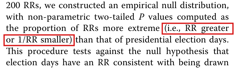S2) The empirical null distribution, the $P$ value and the interval (Methods, Page 2 of 3): “To assess statistical significance, we estimated RRs for the 100 Tuesdays before and after presidential election days. (We restrict ourselves to Tuesdays as all United States presidential elections are held on Tuesdays, thus conditioning on any day-of-week effects.) Using these 200 RRs, we constructed an empirical null distribution, with non-parametric two-tailed $P$ values computed as the proportion of RRs more extreme (i.e., RR greater or 1/RR smaller) than that of presidential election days. This procedure tests against the null hypothesis that election days have an RR consistent with being drawn randomly from the distribution of Tuesdays [3]. We further calculated 95 % Wald-type confidence intervals (CIs) under a normal approximation using the standard deviation of the empirical null distribution as an estimate of the standard error. 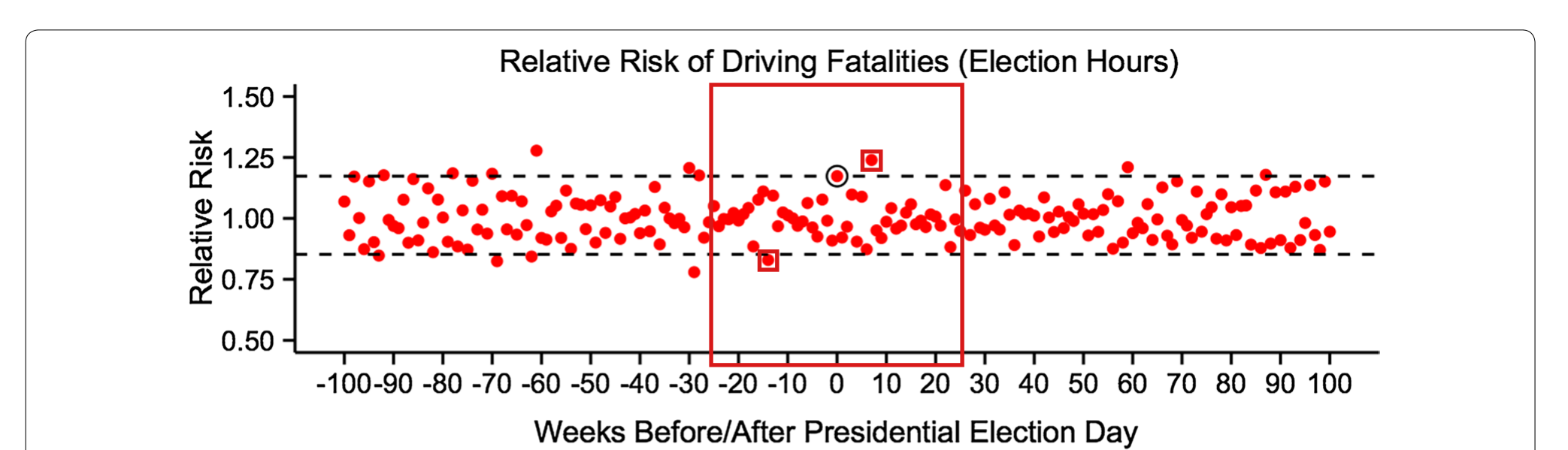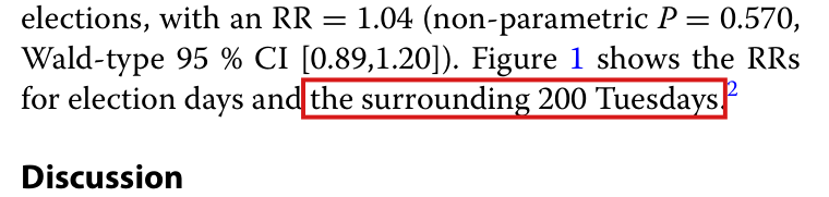Throughout, we consider only presidential elections from 1980 through 2008, as data were not available before 1975 or after 2012, precluding estimation for all Tuesdays surrounding the 1976 or 2012 elections.” (S3) Fig. 1 (Page 2 of 3): three panels, titled “Relative Risk of Driving Fatalities (Election Hours)”, “Relative Risk of Driving Fatalities (Non-Election Hours)” and “Relative Risk of Driving Fatalities (Full 24 Hours)”, each with vertical axis “Relative Risk” (ticks 0.50, 0.75, 1.00, 1.25, 1.50) and horizontal axis “Weeks Before/After Presidential Election Day” (ticks −100 to 100 in steps of 10). Caption: “Fig. 1 Relative risk (RR) estimates for presidential election days and the 100 preceding and following Tuesdays. Red dots indicate RRs for all Tuesdays. Black circles indicate RRs and black dashed lines indicate RR and 1/RR for presidential election days. The proportion of red dots outside black dashed lines is equivalent to the reported non-parametric $P$ value”. 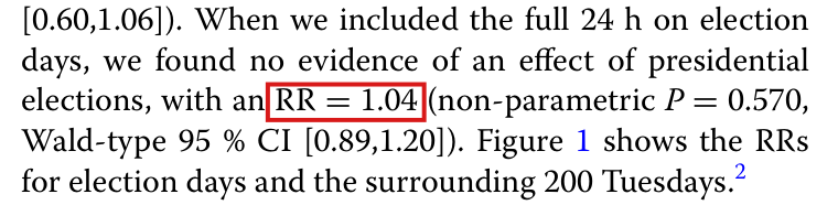(S4) The main results (Results, Page 3 of 3): “We estimate an RR for election hours during presidential elections from 1980 to 2008 of 1.17 (non-parametric $P = 0.070$, Wald-type 95 % CI [0.99,1.35]).” “Furthermore, we estimate an equally strong negative effect of presidential elections on driving fatalities during non-election hours on election days, with an RR = 0.83 (non-parametric $P = 0.085$, Wald-type 95 % CI [0.60,1.06]). When we included the full 24 h on election days, we found no evidence of an effect of presidential elections, with an RR = 1.04 (non-parametric $P = 0.570$, Wald-type 95 % CI [0.89,1.20]). Figure 1 shows the RRs for election days and the surrounding 200 Tuesdays.” (footnote mark 2). 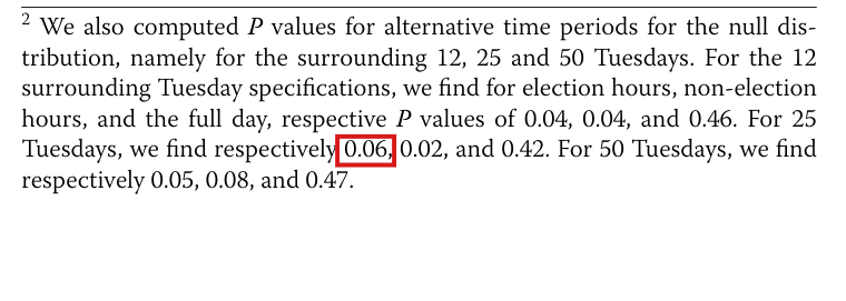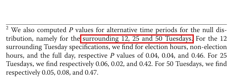(S5) Alternative null windows (footnote 2, Page 3 of 3): “We also computed $P$ values for alternative time periods for the null distribution, namely for the surrounding 12, 25 and 50 Tuesdays. For the 12 surrounding Tuesday specifications, we find for election hours, non-election hours, and the full day, respective $P$ values of 0.04, 0.04, and 0.46. For 25 Tuesdays, we find respectively 0.06, 0.02, and 0.42. For 50 Tuesdays, we find respectively 0.05, 0.08, and 0.47.” Not in the paper or the staged sources: the FARS counts, the plotted RR values as numbers, and any code (the staged manifest records the FARS data as unavailable and no replication code). Every statement below about which reference Tuesdays are ‘more extreme’ is therefore a statement about the published Fig. 1, not about the source data.

Effective claim (source TeX): [Printed; footnote 2, Page 3 of 3] “We also computed $P$ values for alternative time periods for the null distribution, namely for the surrounding 12, 25 and 50 Tuesdays. For the 12 surrounding Tuesday specifications, we find for election hours, non-election hours, and the full day, respective $P$ values of 0.04, 0.04, and 0.46. For 25 Tuesdays, we find respectively 0.06, 0.02, and 0.42. For 50 Tuesdays, we find respectively 0.05, 0.08, and 0.47.” The value at issue is the first of the third sentence: the election-hours $P$ value for the 25-Tuesday window, printed 0.06. [Printed; Fig. 1 caption, Page 2 of 3] “The proportion of red dots outside black dashed lines is equivalent to the reported non-parametric $P$ value”. [Corrected; Sol's smallest_repair, validated.json, P038-N005, verbatim] “Reconcile footnote 2 and Figure 1 against the final data. If Figure 1 is correct, replace the first 25-week value, 0.06, with 0.04. If 0.06 is the verified final-data result, correct the figure to show the requisite third tail point and any other affected plotted quantities; its identity cannot be determined from the staged sources.” Under the first branch the third sentence of footnote 2 reads: “For 25 Tuesdays, we find respectively 0.04, 0.02, and 0.42.” [Mathematical content, with every hypothesis] Notation (not in the paper). Fix one time-of-day category (here election hours). Let $R > 0$ be the election-day RR and, for each integer $w$ with $1 \le |w| \le 100$, let $r_w > 0$ be the RR of the Tuesday $w$ weeks after ($w > 0$) or $-w$ weeks before ($w < 0$) election day. For an integer $m$ with $1 \le m \le 100$ put $W_m = \{w \in \mathbb{Z} : 1 \le |w| \le m\}$, so that $|W_m| = 2m$ and week $0$ is not in $W_m$. Call $r_w$ more extreme than $R$ when it lies outside the dashed lines of Fig. 1, that is, when $r_w < \min(R, 1/R)$ or $r_w > \max(R, 1/R)$. Put $T = \{w : r_w \text{ is more extreme than } R\}$, $k_m = |T \cap W_m|$ and $$P_m = \frac{k_m}{2m}.$$ The main specification is $m = 100$ (200 RRs); footnote 2 is read as $m = 12, 25, 50$ (24, 50 and 100 RRs). A two-decimal number $v$ is the rounding of $x$ when $v - \tfrac{1}{200} \le x < v + \tfrac{1}{200}$. (i) [The value the figure gives] For every $R > 0$ and every family $(r_w)_{w \in W_{25}}$ of positive reals of which exactly two are more extreme than $R$ (that is, $k_{25} = 2$), $$P_{25} = \frac{2}{50} = \frac{1}{25} = 0.04 .$$ (ii) [What the printed value requires] For every integer $k$ with $0 \le k \le 50$: $\frac{k}{50} = \frac{6}{100}$ if and only if $k = 3$; $\frac{k}{50}$ rounds to $0.06$ if and only if $k = 3$; and $\frac{k}{50}$ rounds to $0.04$ if and only if $k = 2$. Consequently $P_{25}$ equals (equivalently, rounds to) the printed $0.06$ if and only if exactly three of the fifty reference RRs are more extreme than $R$, and equals $0.04$ if and only if exactly two are. The two published outputs (footnote 2: $0.06$; Fig. 1: two reference points outside the lines) therefore cannot both be right; they differ by $\frac{6}{100} - \frac{1}{25} = \frac{1}{50}$, one tail point in fifty. (iii) [The 12-Tuesday value agrees with the same figure] $k_m \le k_{m'}$ whenever $m \le m'$. If $T \cap W_{25} = \{-14, 7\}$ (the two tail points of the election-hours panel), then $k_{12} = 1$ and $k_{25} = 2$, so $P_{12} = \frac{1}{24}$, which rounds to the printed $0.04$ because $\frac{35}{1000} \le \frac{1}{24} < \frac{45}{1000}$, while $P_{25} = 0.04$ and does not round to $0.06$. (iv) [Counting the election day itself does not reconcile them] If the election-day point were counted as one more extreme observation among $2m + 1$ points, the 25-Tuesday value would be $\frac{k_{25} + 1}{51} = \frac{3}{51} = \frac{1}{17}$, which rounds to $0.06$ because $\frac{55}{1000} \le \frac{1}{17} < \frac{65}{1000}$; but the 12-Tuesday value would be $\frac{k_{12} + 1}{25} = \frac{2}{25} = 0.08$, which does not round to the printed $0.04$. So with $T \cap W_{25} = \{-14, 7\}$ neither convention gives both printed election-hours values ($0.04$ for 12 Tuesdays and $0.06$ for 25).

: SAP.P038.T1Statement

Theorem: SAP.P038.T1

Statement hash: 67d0396bc062cfd2a75d01721ad57832d9809bd1119bf34e5d8c9deab556f573

Statement definition: SAP.P038.T1Statement

Certificate. 20261103T230038Z

Declaration review: faithful; 2026-11-04T12:48:03Z; binding v2

Evidence scope: Certification checks formal proof objects. Statement fidelity is a model judgment. Author review is separate.

Proof dependencies: Independently extracted

Source and evidence metadata · sap-2026-11-08-assured-release

Reproduction

What I recalculated or reran from public materials. "Agrees", "Agrees in part" or "Disagrees" compares my result with the printed one. "Not compared" means the comparison could not be made.

Status: Selected recalculation
Agreement: Agrees in part

Reported results that were targeted
Target	Where	Method	Status	Agreement
Election-hours estimate	Results, article p. 3 (PDF p. 3)	I read the election-day RR from Figure 1, counted 14 of 200 reference RRs outside the dashed lines, and recalculated the interval from the plotted reference RRs. The displayed RR 1.17, P = 0.070 and interval [0.99, 1.35] agree to rounding. Recalculation from FARS data remains blocked by missing data and code.	Recalculated	To rounding
Non-election-hours estimate	Results, article p. 3 (PDF p. 3)	I read the election-day RR from Figure 1, counted 17 of 200 reference RRs outside the dashed lines, and recalculated the interval from the plotted reference RRs. The displayed RR 0.83, P = 0.085 and interval [0.60, 1.06] agree to rounding. Recalculation from FARS data remains blocked by missing data and code.	Recalculated	To rounding
Full-day estimate	Results, article p. 3 (PDF p. 3)	I compared the printed RR, P value and interval with Figure 1. The plotted RR agrees with 1.04, and 113 or 114 of 200 reference points lie outside the lines, compatible with P = 0.570. The interval recalculated from the figure has upper limit about 1.19; the figure’s resolution cannot distinguish this from the printed 1.20. Recalculation from FARS data remains blocked. The partial-agreement label records this unresolved precision limit; I did not establish a discrepancy in the full-day results.	Recalculated	Agrees in part
Figure 1	Article p. 2 (PDF p. 2), three panels and caption	I compared the three plotted election-day RRs and their reciprocal dashed lines with the printed RRs 1.17, 0.83 and 1.04, and counted 201 points per panel. These features agree to rounding; I did not regenerate the figure from FARS data. The estimate rows describe the P-value and interval comparisons.	Recalculated	To rounding
Binomial-test rejection rate	Results, article p. 3 (PDF p. 3), first paragraph	I checked only that 43% is attainable as 86 of 200. I did not recompute the tests or compare an independently calculated rejection rate: the pooled counts, rejection threshold, test convention and analysis code are unavailable.	Blocked	Not compared
Alternative-window P values	Footnote 2, article p. 3 (PDF p. 3)	I counted points outside the dashed lines of Figure 1 in the shorter windows. Eight of the nine footnote values agree to rounding; election hours with 25 Tuesdays on each side gives 2/50 = 0.04, against 0.06 (P038-N005). Only the election-hours counts for 12 and 25 Tuesdays were repeated independently. The final data are needed to choose whether the figure or footnote should change.	Recalculated	Agrees in part