Journal article P040

Corrections to: Chocolate Scents and Product Sales: A Randomized Controlled Trial in a Canadian Bookstore and Cafe

Mary C. McGrath, P. M. Aronow, and Vivien Shotwell (2016). Chocolate Scents and Product Sales: A Randomized Controlled Trial in a Canadian Bookstore and Cafe. SpringerPlus 5:670.

DOI: 10.1186/s40064-016-2303-5
Audited edition: SpringerPlus, 2016, 5:670; 6 pages in the audited file
SHA-256 of the audited file: fb4688bfbb6b51f295d941f9284bea6606e2466870c096b474f2e6e62e3da64d
Permanent address: https://pmaronow.github.io/llm-audit/works/P040/

Summary

The paper reports a randomized trial of chocolate scent in a Canadian bookstore with an adjoining café, which replicates and extends a 10-day Belgian study. Over a 31-day period, days were assigned by coin flip to scent or to no scent; the sales analysis uses 30 daily observations. No effect on daily sales is statistically detectable. 4 entries are classified as errors (1 Moderate, 3 Minor); 4 other concerns were not confirmed, 3 remain unresolved and 1 falls outside this audit’s scope. The manipulation check’s lower-Wald-endpoint interpretation is conventional, but the reconstructed normal approximation is poorly calibrated with 15 responses (P040-E001). Under independent sampling with a common detection probability, exact binomial uncertainty is wider; the observed 14 of 15 spontaneous or prompted detections and the sales computations remain.

What was and was not checked

I checked the following recalculations from version 2.0 of the replication files, with the qualifications below. Running the sales script required changes to file locations, a filename and graphics output.

Table 1: the analysis script, run on the 30 daily observations, reproduces the 16 estimates and the 16 standard errors to the printed decimal, for example $575.4$ $(34.7)$ and $36.6$ $(51.6)$ for total sales without adjustment.
Table 1 is consistent with itself: the control means of the three categories sum to the control mean of total sales ( $72.0 + 334.7 + 168.7 = 575.4$ ), and the three effects sum to the total effect within rounding.
The unadjusted coefficients equal the differences between the treatment and control means, as the paper states on p. 4. The robust standard errors are the HC1 standard errors. The adjusted regression centres the time trend and the day-of-week indicators as described, and it has rank 9 and 21 residual degrees of freedom.
No estimate of a treatment effect is significant at the two-tailed $.10$ level: the smallest of the eight $p$ -values is $.215$ with the normal reference and $.225$ with the Student- $t$ reference. This holds in both columns of Table 1, in agreement with the statement that the findings are not substantively altered by adjusting for time trends.
The recorded assignment coding agrees with the stated rule: the treatment indicator equals one exactly when the recorded random number exceeds $.5$ , on all 30 days, of which 16 are treatment days and 14 are control days.
“three times as many observations” as the original study: 30 days against 10.
In all 30 rows of the sales data, total book sales are the sum of new and remaindered book sales, and total sales are the sum of book, café and bulk sales.
Fig. 1: a redrawing from the sales data matches the printed markers, with none at day 5, to the precision of a comparison by eye. The 16 gray bars fall on the 16 treatment days of the data.
The counts of the manipulation check on p. 3 agree with the data: six spontaneous detections, 14 of 15 detections when prompting is included, six spontaneous identifications as chocolate and five further recognitions. The printed interval agrees with the reconstructed normal-approximation interval. The small-sample calibration of that approximation is the subject of P040-E001.
The adjusted means and effects for café and bulk sales quoted on p. 5 agree with Table 1, and their $p$ -values agree with the Student- $t$ tests of the analysis script; see P040-E003.
The conclusion on countervailing effects, p. 5: contrasts of combined café and bulk sales with book sales, which the paper does not report, are not statistically significant in either regression.

I checked the whole article, its footnotes, its references and the replication files by reading them. The Conclusions acknowledge limited power and several differences between the two settings that cannot be separated, and they state that the results do not preclude an effect of chocolate scent. I consulted sources outside the paper on two points: a chapter of the doctoral dissertation of the first author of the original study, for the method of that study, and bibliographic entries for Doucé et al. (2013) and for Herrington (1996), for P040-N008. The entries confirm two misprints in the Doucé reference; conflicting entries leave Herrington’s author list unresolved.

I did not read the cited journal articles or compare the following with those sources: the increases of 5.07%, 22% and 40% in the original study, the quotations, and the estimator of Lin (2013). I compared the original study’s design with the dissertation chapter only. Its 201 observed entrants over 10 days, with every fifth entrant selected, are consistent with roughly 100 entrants per day; this is a reconstruction, not an independently measured daily total. I did not compare the heights of the markers in Fig. 1 with the data exactly. The replication files contain no code for the interval of the manipulation check; the Wald formula reproduces its limits, but the precise command used remains unknown. I used only version 2.0 of the replication files. I found no appendix or supplementary-file notice in the article, and I did not search for a published correction.

Four study details remain unresolved. The sales data have no entry for August 5 (P040-E002); this does not establish how many days were originally assigned conditions or why August 5 is absent. The dates and conditions of the manipulation-check survey are not given. The annotation “Pan-only” on one control day of the sales data is not defined. The rule by which the 21 customers per day were counted is not stated. I could not settle the last three without further information from the authors. These checks do not show that the paper is correct in the respects that were not examined.

Headline claims and related corrections

A randomized trial of chocolate scent in a Canadian bookstore with an adjoining café finds no evidence that the scent affects total sales: the estimated effect is positive but not statistically significant.
Table 1, rows 'Total sales'; Fig. 1; abstract (PDF p. 1), Background (p. 2), Results (p. 4), Conclusions (p. 5)
See P040-E001, P040-E003.
The paper reports no effect within the sales categories: none of the estimated effects on bulk, café or book sales is significant at two-tailed $p<.10$ . In the adjusted analysis, café sales fall by $8.9$ CAD ( $p=.59$ ) and bulk sales rise by $23.2$ CAD ( $p=.29$ ).
Table 1, rows 'Bulk sales', 'Café sales', 'Book sales'; Results, PDF pp. 4-5; Conclusions, PDF p. 5
See P040-E003, P040-E001.
There is no evidence of countervailing effects, that is, that the scent raised sales of within-domain products (food items) or shifted purchases from out-of-domain products (books) toward them.
Table 1 (café, bulk and book rows compared); Results, PDF p. 5, left column; Conclusions, PDF p. 5
The findings are not substantively altered by adjusting for a linear time trend and day-of-week fixed effects.
Table 1, column 'Adjusted for time trends'; Results, PDF p. 4, right column
The paper describes a 31-day randomized replication and extension of a 10-day bookstore experiment, with each experimental day independently assigned to chocolate scent or no scent with probability $.5$ , giving three times as many experimental-day observations as the original study.
Methods, PDF pp. 2-3; abstract, PDF p. 1; Fig. 1 and caption, PDF p. 4; replication data and R script
See P040-E002.
The paper reports that $93\%$ of 15 sampled customers detected a scent, with a $95\%$ confidence interval of $.81$ to $1.06$ . It interprets the lower endpoint as indicating that at least $80\%$ of patrons would discern the scent and concludes that the scent was sufficiently detectable.
Results and discussion, PDF p. 3, right column (manipulation-check paragraphs); manipulation_check_data.dta
See P040-E001.
The findings show the value of replication in varied settings: contextual factors and the choice set may moderate scent effects; the null result could reflect a spurious original association, a baseline already boosted by café scents, other differences between the two studies, or low power, and does not preclude an effect.
Abstract, PDF p. 1; Background, PDF p. 2; Conclusions, PDF p. 5; Table 1 as a whole

Corrections

Moderate (1)

A real substantive error with limited reach.

P040-E001 Moderate

The printed interval agrees with a nominal Wald interval with a conventional lower-endpoint interpretation, but its normal approximation is poorly calibrated with 15 responses: exact coverage at a detection probability of $.80$ is about 81.5%.

Results and discussion, third paragraph, p. 3 (PDF p. 3), right column: the interval “(95 % CI: .81, 1.06)” and the last sentence of the paragraph

See also under Formal statements (Lean): P040-T1, P040-T2

I disputed this classification, but as a rule, deferred to the models’ final judgment: see my comment and the history of this entry.

As printed

In our sample of 15 customers, six spontaneously detected a scent. Once prompted to consciously attend to scent, all but one of the respondents were able to discern the presence of an ambient scent. Six respondents spontaneously identified that ambient scent as chocolate, and another five reported recognizing the scent as chocolate once the enumerator identified the scent as such. The total proportion of our sample reporting a detectable ambient scent was .93 (95 % CI: .81, 1.06). One limitation of the small sample size in our manipulation check is that the confidence intervals for our estimates are relatively wide. However, since the lower bound of our estimate indicates that at least 80 % of patrons would discern the presence of an ambient scent, we remain confident that the scent was sufficiently detectable.

The problem

The count is correct: 14 of the 15 respondents detected a scent, spontaneously or when prompted, and $14/15\approx .93$ . The paper does not name its interval method. The printed limits agree with the normal-approximation, or Wald, interval $\hat p\pm z_{.975}\sqrt{\hat p(1-\hat p)/n}$ , where $z_{.975}\approx1.96$ is the standard normal $.975$ quantile, $\hat p=14/15$ and $n=15$ ; this gives approximately $(.807,1.060)$ . Reading its lower endpoint as approximate confidence-based evidence for a population detection rate above $.80$ is conventional. The passage does not promise certainty or exact finite-sample coverage, and this interpretation is not the defect.

The defect is the approximation’s accuracy in this small sample. Under independent common-probability Bernoulli responses with $n=15$ and $p=.80$ , the reconstructed nominal 95% interval contains $p$ with probability only $.8148$ , and its lower limit is at most $p$ with probability only $.8329$ . By contrast, with fixed $0<p<1$ and increasing $n$ , those probabilities tend to $.95$ and $.975$ . The finite-sample failure does not refute that asymptotic interpretation.

The nominal Wald test does reject $.80$ here, with a two-sided normal $P$ value of about $.03843$ . The exact one-sided binomial tail probability is about $.16713$ . An exact equal-tailed 95% interval rounds to $[.68,1.00]$ , and an exact one-sided 95% lower limit rounds to $.72$ . These alternatives show the weaker assurance available without the unreliable normal approximation. An upper limit above one is not by itself the error: clipping the printed interval at one changes neither its lower limit nor its coverage for a permissible probability.

Evidence an exact counterexample

I checked the Wald derivation, calculated finite-sample coverage exactly and recalculated the counts from the replication files. The manipulation-check file has 15 respondents, of whom 14 detected a scent. For the calculations, suppose that the 15 responses are independent with a common detection probability $p$ , so that the number $X$ of detections is binomial with parameters $15$ and $p$ . I assume this sampling model for the calculations; the paper does not specify its interval method.

For fixed $0<p<1$ , the Bernoulli central limit theorem and consistency of $\hat p$ give

\frac{\sqrt n(\hat p-p)}{\sqrt{\hat p(1-\hat p)}}\;\xrightarrow{d}\;N(0,1).

Consequently the nominal two-sided Wald interval has coverage tending to $.95$ , and its lower endpoint is an approximate one-sided 97.5% lower confidence limit. This supplies the conventional approximate reading; it gives no small-sample accuracy bound at $n=15$ .

Now fix $p=4/5$ and $n=15$ . Then

\mathbb{P}(X = 14) = 15 \left(\frac{4}{5}\right)^{14} \frac{1}{5} = \frac{805306368}{6103515625} \approx .1319 .

The printed interval at $X = 14$ excludes $.80$ ; if $.81$ is a rounded value, the limit is still at least $.805$ . Consider any rule that assigns an interval to each count and assigns the printed interval to the count 14. This rule fails to contain $p = .80$ whenever $X = 14$ , which implies that it contains $.80$ with probability at most $1 - .1319 = .8681$ . This probability is less than $.95$ , and the bound does not depend on the method that produced the interval. It refutes an exact finite-sample 95% guarantee for a deterministic count-only rule with that endpoint, not the usual asymptotic interpretation of a Wald endpoint. For the normal-approximation rule, the interval contains $.80$ exactly when $9 \le X \le 13$ , so

\mathbb{P}(9 \le X \le 13) = \frac{24866193408}{30517578125} \approx .8148 .

Exact probabilities for 15 independent responses with detection probability $.80$ . The rule in the last two rows is the nominal normal-approximation interval $\hat p \pm 1.96 \sqrt{\hat p (1 - \hat p)/15}$ .
Event	Probability	Decimal
$X = 14$	$805306368/6103515625$	$.1319$
$X \ge 14$	$5100273664/30517578125$	$.1671$
The interval of the rule contains $.80$ ( $9 \le X \le 13$ )	$24866193408/30517578125$	$.8148$
The lower limit of the rule is at most $.80$ ( $X \le 13$ )	$25417304461/30517578125$	$.8329$

For the exact limits, a direct computation gives

\mathbb{P}_p(X \ge 14) = 15 p^{14} (1 - p) + p^{15} = p^{14} (15 - 14 p) .

This function of $p$ is continuous and strictly increasing on $[0, 1]$ , since its derivative is $210 p^{13} (1 - p)$ . The lower limit $L$ of the exact equal-tailed 95% interval is the solution of $L^{14} (15 - 14 L) = .025$ . The upper limit $U$ is the solution of $\mathbb{P}_U(X \le 14) = 1 - U^{15} = .025$ . The exact one-sided 95% lower limit $L_1$ is the solution of $L_1^{14} (15 - 14 L_1) = .05$ . Their solutions are

L \approx .680515, \qquad U \approx .998314, \qquad L_1 \approx .720604 .

For every $p$ , the lower limit of the exact interval exceeds $p$ with probability at most $.025$ , and its upper limit is less than $p$ with probability at most $.025$ . This implies that the interval contains $p$ with probability at least $.95$ . At $p=.80$ , $\mathbb{P}(X \ge 14) \approx .1671$ , which exceeds $.05$ and $.025$ .

What survives

The observed count of 14 detections among 15, the other manipulation-check counts, the reconstructed Wald arithmetic and the conventional lower-confidence-endpoint interpretation survive. The sales regressions, Table 1 and Fig. 1 do not use the survey responses or the interval, so this repair leaves their numerical calculations unchanged; it does not independently validate that analysis.

The surveyed sample has a high observed detection rate. Under the exact-binomial alternative its 95% interval extends down to about $.68$ , and its one-sided 95% lower limit is about $.72$ . The nominal Wald inference above $.80$ therefore remains a conventional but poorly calibrated approximation here. Nothing establishes that the true rate is below $.80$ or that the scent was too weak.

Corrected

Fourteen of the fifteen surveyed customers reported detecting an ambient scent, either spontaneously or after prompting. Under an independent common-probability binomial sampling model, the exact equal-tailed 95% confidence interval is approximately $[.680515, .998314]$ . The observed detection rate was high, but the exact-binomial lower endpoint is about $.68$ rather than above $.80$ , leaving substantial uncertainty about the detection rate; generalization beyond the surveyed customers requires appropriate sampling assumptions.

The exact-binomial alternative can be specified as follows. Let $X$ be the number of detections among $n = 15$ respondents, and suppose that the responses are independent with a common detection probability $p \in [0, 1]$ , so that $X$ is binomial with parameters $15$ and $p$ . For the observed value $X = 14$ , the exact equal-tailed 95% confidence interval for $p$ is $[L, U]$ , where $L$ and $U$ are the unique solutions in $(0, 1)$ of

L^{14} (15 - 14 L) = .025, \qquad U^{15} = .975 .

Then $L \approx .680515$ and $U \approx .998314$ , and at the precision of the paper the interval is $[.68, 1.00]$ . The exact one-sided 95% lower confidence limit is the unique solution $L_1 \approx .720604$ in $(0, 1)$ of $L_1^{14} (15 - 14 L_1) = .05$ . Both lower limits are less than $.80$ . These limits concern the detection probability under the stated model. A statement about patrons in general requires in addition that the 15 respondents represent them, and the paper does not describe how the respondents were selected.

Crop of the fifteen lines of the paragraph. The text reads: In our sample of 15 customers, six spontaneously detected a scent. Once prompted to consciously attend to scent, all but one of the respondents were able to discern the presence of an ambient scent. Six respondents spontaneously identified that ambient scent as chocolate, and another five reported recognizing the scent as chocolate once the enumerator identified the scent as such. The total proportion of our sample reporting a detectable ambient scent was .93 (95 \% CI: .81, 1.06). One limitation of the small sample size in our manipulation check is that the confidence intervals for our estimates are relatively wide. However, since the lower bound of our estimate indicates that at least 80 \% of patrons would discern the presence of an ambient scent, we remain confident that the scent was sufficiently detectable. One red outline surrounds (95 \% CI: .81, 1.06) and a second surrounds the words at least 80 \% of patrons. — Results and discussion, third paragraph, p. 3 (PDF p. 3), right column. The outlines mark the printed interval, “(95 % CI: .81, 1.06)”, and the inference drawn from its lower limit, “at least 80 % of patrons”.

Chart with one horizontal axis for the detection probability p, with labelled ticks from .60 to 1.10, and three horizontal bars. The title reads: 14 of 15 customers detected a scent: the exact 95\% lower limits, .68 and .72, are below the printed limit .81 and below the minimum of .80 that the paper states. The top bar, in orange, is labelled As printed: 95 \% CI (.81, 1.06); its endpoints are approximately .807 and 1.060, labelled .81 and 1.06, and it extends into a gray region to the right of 1.00 that is labelled above 1: not a probability. The middle bar, in blue, is labelled Exact 95\% interval, equal tails; its endpoints are labelled .681 and .998. The bottom bar, in blue, is labelled Exact one-sided 95\% lower limit; its lower endpoint is labelled .721 and it ends at 1.00. A dashed vertical line at .80 is labelled stated minimum: .80. The orange bar lies entirely to the right of this line, and both blue bars cross it. An open circle on each bar marks the observed proportion 14/15, labelled .933. — The nominal interval as printed and the exact binomial limits for 14 detections among 15 respondents, on one axis for the detection probability $p$ . The printed interval $(.81, 1.06)$ is drawn at the endpoints, approximately $.807$ and $1.060$ , of the nominal normal-approximation interval. Its lower-endpoint interpretation is conventional, while the exact finite-sample calculation exposes poor calibration here. The exact equal-tailed 95% interval rounds to $[.681, .998]$ , and the exact one-sided 95% lower limit rounds to $.721$ . Both exact lower limits lie to the left of the dashed line at $.80$ . The open circles mark the observed proportion $14/15$ .

My comment and the history of this entry

I agree that what is proposed is a better analysis, but this is a standard interpretation of a asymptotic Wald-type interval (even if the asymptotics weren't warranted).

Suggested classification: Minor error.

My position My comment above; I suggested a Minor error.

The models’ position For the reconstructed nominal 95% Wald interval, with 15 independent responses and a common detection probability of .80, two-sided coverage is only about 81.5%. The conventional reading of its lower endpoint was accepted, but the paper’s explicit assurance of at least 80% rests on a seriously inaccurate small-sample approximation: Moderate.

Classification before my review (the classification when the audit was first completed, before I reviewed it): Moderate error.
I commented and suggested a Minor error.
Independent evaluation. Incorporated in part. The claims that .81 cannot be a nominal 95% limit and that the paper misread its interval were withdrawn, and the entry was redrafted around the interval’s poor calibration in small samples. My suggested rating (Minor) was not adopted.

Minor (3)

Real but inconsequential, for example a misprint that does not change a result.

P040-E002 Minor

The reported analyses and Fig. 1 cover 30 daily observations, for August 1–4 and August 6–31: the trial spanned 31 calendar days, and the replication data have no entry for August 5.

Methods, first sentence on p. 3 (PDF p. 3), left column; Fig. 1 and its caption, p. 4 (PDF p. 4)

As printed

p. 3, Methods. The trial used a between-subjects design in which the 31 experimental days were assigned one of two conditions: chocolate scent dispersion (treatment) and no scent (control). Condition was determined by Bernoulli (coin flip) random assignment with probability .5 independently across days.

p. 4. We present the complete raw results of the trial in Fig. 1.

p. 4, caption of Fig. 1. All sales data associated with the randomized controlled trial. The x-axis shows each of the 31 days of the experiment, with gray vertical bars indicating days on which the chocolate scent was administered.

The problem

The paper states that there were 31 experimental days, and it presents Fig. 1 as the complete raw results, on an axis that shows each of the 31 days. In a trial randomized by day, this suggests that the daily data and the analysis cover 31 observations. The replication data hold 30 daily observations, for August 1–4 and August 6–31, of which 16 are treatment days and 14 are control days. August 5 is absent. The analysis script uses the 30 rows without removing or adding any, and Fig. 1 has no markers at day 5. The paper does not distinguish the 31-day span from the 30 observed days, and it does not explain why August 5 is absent.

Evidence a recalculation from the source

I checked the replication files. The daily sales file has 30 distinct dates, each with complete values of the four outcomes. Computing the eight regressions of the analysis script from these 30 rows in exact arithmetic, I obtain the 16 estimates and the 16 standard errors of Table 1 to the printed decimal. The files do not show whether August 5 was assigned a condition, whether sales were recorded on that day, or why the day is absent. It is not established that only 30 days were randomized, and no change in an estimate and no selection effect is established.

What survives

Table 1, the 30 plotted days of Fig. 1 and the conclusions on sales are unchanged. The descriptions of a 31-day trial in the abstract and on p. 2 hold for the calendar span, August 1–31, and the statement on p. 3 that the study has three times as many observations as the original 10-day study holds for 30 days. The correction clarifies the report.

Corrected

p. 3, Methods, to be added. The trial period spanned August 1–31. The reported analyses use 30 daily observations (August 1–4 and August 6–31), comprising 16 treatment and 14 control days. August 5 is absent from the deposited sales data.

p. 4, caption of Fig. 1. All sales data associated with the randomized controlled trial. The x-axis spans the 31-day trial period. Markers show the 30 observed days; no observation is shown for day 5. Gray vertical bars indicate observed days assigned to the chocolate-scent treatment.

The number of days that were assigned a condition and the reason for the absence of August 5 should be stated from the trial records, if these are available. The evidence does not support the replacement of “31 experimental days were assigned” by “30 experimental days were assigned”.

Crop of six lines of the left column of page 3. The text reads: The trial used a between-subjects design in which the 31 experimental days were assigned one of two conditions: chocolate scent dispersion (treatment) and no scent (control). Condition was determined by Bernoulli (coin flip) random assignment with probability .5 independently across days. The crop ends with the fragment Chocolate scent was dispersed. A red outline surrounds the words 31 experimental days. — Methods, first sentence on p. 3 (PDF p. 3), left column. The outline marks “31 experimental days”.

Crop of Fig. 1, titled Sales by Type on Treatment and Control Days. The horizontal axis is Day of Experiment, with ticks from 0 to 30, and the vertical axis is Sales in Canadian Dollars, from 0 to 1000. Each observed day has four markers: a circle for total sales, an X for cafe sales, a diamond for book sales and a triangle for bulk sales. Sixteen gray vertical bars mark the treatment days. A tall red outline surrounds the column of the plot at day 5 and the tick label 5 below it; the column is empty. In the caption below the figure, a second red outline surrounds the words 31 days of the experiment. The caption reads: Fig. 1 Sales by type on treatment and control days. All sales data associated with the randomized controlled trial. The x-axis shows each of the 31 days of the experiment, with gray vertical bars indicating days on which the chocolate scent was administered. The y-axis shows sales in Canadian dollars (CAD). The markers indicate sales per day: circles denote total sales, Xs denote cafe sales, diamonds denote book sales, and triangles denote bulk coffee bean/loose tea/spice sales. — Fig. 1 with its caption, p. 4 (PDF p. 4). The outline in the caption marks “31 days of the experiment”. The outline in the plot marks the position of day 5, where no markers are plotted; every other day from 1 to 31 has four markers.

P040-E003 Minor

The printed $p$ -values are computed from a Student- $t$ reference distribution with the residual degrees of freedom of each regression, 28 for the unadjusted regressions and 21 for the adjusted regressions, and not under a normal approximation.

p. 4 (PDF p. 4), left column, first paragraph, last sentence; the two $p$ -values that it governs, p. 5 (PDF p. 5), left column, last paragraph

See also under Formal statements (Lean): P040-T4, P040-T5

As printed

p. 4. In all cases, robust standard errors are used to estimate standard errors, with $p$ values computed under a normal approximation.

p. 5. The direction of the treatment effect on café sales was slightly negative, though not statistically significant (average estimated decrease of 8.9CAD from a control average of 336.5CAD, two-tailed $p = .59$ ) and the direction of treatment on bulk coffee bean/loose tea/spice sales was slightly positive, though not statistically significant (average estimated increase of 23.2CAD from a control average of 71.2CAD, two-tailed $p = .29$ ).

The problem

The Methods state that the $p$ -values are computed under a normal approximation. For an estimate with ratio $t$ to its robust standard error, this is the value $2 \Phi(-|t|)$ , where $\Phi$ is the standard normal distribution function. The analysis script instead computes each $p$ -value from the Student- $t$ distribution with the residual degrees of freedom of the regression, which are 28 for the unadjusted regressions and 21 for the adjusted regressions. The two values printed on p. 5 are these Student- $t$ values. Under the normal approximation they are $.58$ and $.28$ .

Evidence an exact counterexample

I checked a recalculation from the replication files. With its statistical expressions unchanged, the analysis script reproduces all 32 estimates and standard errors of Table 1 to the printed decimal. Its test of coefficients uses the residual degrees of freedom of the fitted regression. The robust standard errors of the script are the HC1 standard errors. The two adjusted effects were also computed in exact arithmetic, with certified bounds for the two probabilities.

The two adjusted treatment effects quoted on p. 5: the estimate and its robust standard error in CAD, their ratio $t$ , and the two-tailed $p$ -value under the Student- $t$ distribution with 21 degrees of freedom and under the standard normal distribution.
Outcome	Estimate	Standard error	$t$	$p$ , Student- $t$	$p$ , normal	Printed
Café sales	$-8.891$	$16.151$	$-0.5505$	$.5878$	$.5820$	$.59$
Bulk sales	$23.179$	$21.247$	$1.0909$	$.2877$	$.2753$	$.29$

The Student- $t$ values round to the printed $.59$ and $.29$ , and the normal values round to $.58$ and $.28$ . The normal value for bulk sales must be computed from the unrounded estimate and standard error. With the rounded entries $23.2$ and $21.2$ of Table 1, I obtain a value near $.274$ .

What survives

The estimates and standard errors of Table 1 and the observations of Fig. 1 are unchanged. No statement of significance changes. Over the eight tests of a treatment effect, the smallest $p$ -value is $.225$ with the Student- $t$ reference and $.215$ with the normal reference. The statement on p. 4 that no estimate is significant at the two-tailed $.10$ level holds in both cases. The correction changes the description of the method.

Corrected

p. 4. In all cases, robust standard errors are used to estimate standard errors, with $p$ values computed using a Student- $t$ reference distribution with the model’s residual degrees of freedom (28 for the unadjusted regressions and 21 for the adjusted regressions).

In full, the corrected statement is the following. For an estimate with ratio $t$ to its robust standard error, the two-tailed $p$ -value is $2\,\mathbb{P}(T_\nu \ge |t|)$ , where $T_\nu$ has the Student- $t$ distribution with $\nu = 30 - k$ degrees of freedom, and $k$ is the rank of the regression on the 30 daily observations. Without covariates, $k = 2$ and $\nu = 28$ . With the linear time trend and the day-of-week effects, $k = 9$ and $\nu = 21$ . The Student- $t$ distribution serves as a reference distribution: the corrected sentence does not state that the ratio has this distribution exactly under the null hypothesis. With this sentence, the two $p$ -values on p. 5 stand as printed. The alternative is to keep the sentence on p. 4, compute the tests with the normal reference, and print $p = .58$ and $p = .28$ on p. 5.

Crop of eight lines of the left column of page 4. The text reads: between treatment and control. To improve efficiency, the second strategy uses ordinary least squares adjusting for a mean-centered linear time trend as well as mean-centered fixed effects for the day of week, following Lin (2013). In all cases, robust standard errors are used to estimate standard errors, with p values computed under a normal approximation. We present the complete raw results of the trial in. A red outline surrounds the words a normal approximation. — p. 4 (PDF p. 4), left column, end of the first paragraph. The outline marks “a normal approximation”.

Crop of eight lines of the left column of page 5. The text reads: ment effect on café sales was slightly negative, though not statistically significant (average estimated decrease of 8.9CAD from a control average of 336.5CAD, two-tailed p = .59) and the direction of treatment on bulk coffee bean/loose tea/spice sales was slightly positive, though not statistically significant (average estimated increase of 23.2CAD from a control average of 71.2CAD, two-tailed p = .29). One red outline surrounds p = .59) and a second surrounds p = .29) and the final period. — p. 5 (PDF p. 5), left column, end of the last paragraph. The outlines mark the two printed $p$ -values, $.59$ for café sales and $.29$ for bulk sales.

P040-N008 Minor

In the reference to Doucé et al. (2013), the title should read “the effect of chocolate scent on purchase-related behavior in a bookstore”, and the surname of the fourth author is De Backer.

References, p. 6 (PDF p. 6), left column, the entry for Doucé et al. (2013)

As printed

Doucé L, Poels K, Janssens W, DeBacker C (2013) Smelling the books: the effect of chocolate scent in purchase-related behavior in a bookstore. J Environ Psychol 36:65–69

The problem

The entry prints “in” where the title of the cited article has “on”, and it prints the surname De Backer as one word.

Evidence a check of the printed page

I checked the page against the bibliographic entry for the cited article in the repository of Hasselt University, which has the title with “on” and the fourth author as “De Backer, Charlotte”. I did not read the article itself. It is not settled whether the entry for Herrington (1996), and footnote 1 on p. 1, omit a second author. The publisher lists J. Duncan Herrington alone, a library catalogue lists Herrington and Capella, and the printed first page of that article was not available.

What survives

The cited work can still be identified from the entry, and nothing in the paper depends on these details.

Corrected

Doucé L, Poels K, Janssens W, De Backer C (2013) Smelling the books: the effect of chocolate scent on purchase-related behavior in a bookstore. J Environ Psychol 36:65–69

Crop of eight lines of the reference list. The first three lines are the entry: Dooley R (2013) Keep your customers shopping... with chocolate! Forbes Available: http://www.forbes.com/sites/rogerdooley/2013/07/22/chocolate-scent/. The next three lines are the entry: Doucé L, Poels K, Janssens W, DeBacker C (2013) Smelling the books: the effect of chocolate scent in purchase-related behavior in a bookstore. J Environ Psychol 36:65 to 69. The last two lines are the entry: Herrington JD (1996) Effects of music in service environments: a field study. J Serv Mark 10:26 to 41. One red outline surrounds the name DeBacker, and a second surrounds the word in that follows chocolate scent. — References, p. 6 (PDF p. 6), left column: the entry for Doucé et al. (2013), between the entries for Dooley (2013) and Herrington (1996). The outlines mark “DeBacker” and the word “in” of the title.

Formal statements (Lean)

Formal results: 5 whole; 0 restricted; 0 refuted; 0 omitted.

Coverage concerns the identified claim under its stated assumptions. A checked proof establishes the formal statement; correspondence to the published text was reviewed by AI. Repository access is currently required to open the source links.

Each result links to its current formal statement and proof. “Whole” covers the identified claim under its assumptions; “restricted” covers the stated narrower scope; “refuted” gives a counterexample to the identified assertion; “omitted” has no current theorem. Any named published theorem used as a premise remains an assumption. Browse the formal results for this work.

P040-T1

Results and discussion, manipulation check: ‘.93 (95 % CI: .81, 1.06)’ and the inference ‘the lower bound of our estimate indicates that at least 80 % of patrons would discern the presence of an ambient scent’; the witness (detection probability 4/5 under a binomial model) is the validator's construction and is not in the paper

p. 3 (PDF p. 3; headed ‘Page 3 of 6’), right column, paragraph beginning ‘In our sample of 15 customers’

p. 3, right column, manipulation check (PDF p. 3). Under the independent common-probability binomial model for fifteen detections, the mass of count 14 at p = .80 is .13194139533312. Every deterministic count-based set excluding .80 there, and every lower bound above .80 there, has coverage at most .86805860466688, so cannot guarantee .95 or .975 uniformly. The printed interval and every lower endpoint rounding to .81 exclude .80. The Wald rule with multiplier 1.96 reproduces the printed endpoints, with the stated rational arithmetic and brackets. For every multiplier in [1.9599,1.9601], membership, two-sided coverage .814815425593344, lower coverage .832874232578048 and lower failure probability .167125767421952 have the stated exact values. The actual standard normal .975 quantile exists uniquely in that range and also reproduces the printed endpoints, with prefixes .807099 and 1.059567. This is the canonical finite-sample calibration counterexample under the added binomial model.

Historical component credits

Proved AronowAudit.P040.binomialMass_nonneg Historical support retained; baseline fidelity: ok; manifest: used; used in Solution; Finite-probability helper used within the exported counterexample proofs; not separately invoked.
Proved AronowAudit.P040.binomialMass_total Historical support retained; baseline fidelity: ok; manifest: used; used in Solution; Finite-probability normalization used within the exported bounds; not separately invoked.
Proved AronowAudit.P040.observed_count_mass Historical support retained; baseline fidelity: ok; manifest: used; used in Solution; The binomial sampling law and p=.80 are explicitly part of this validator-constructed target, rather than deductions from the random assignment of experimental days.
Proved AronowAudit.P040.exclude_observed_count_bound Historical support retained; baseline fidelity: ok; manifest: used; used in Solution; The method-free and lower-bound rows already export its required consequences.
Counterexample proved AronowAudit.P040.method_free_counterexample Historical support retained; baseline fidelity: ok; manifest: used; used in Solution; The target A2 explicitly permits arbitrary subsets of R, so the absence of an interval-shape restriction is faithful. The public description supplied in the record accurately restricts the conclusion to an exact finite-sample guarantee.
Counterexample proved AronowAudit.P040.lower_bound_counterexample Historical support retained; baseline fidelity: ok; manifest: used; used in Solution; Exact counterexample here means failure of the auxiliary finite-sample lower-coverage guarantee stated in T1; it does not establish that the actual patron rate is below .80.
Proved AronowAudit.P040.printed_endpoint_excludes_witness Historical support retained; baseline fidelity: ok; manifest: used; used in Solution; The half-open rounding convention is exactly S7; .805>.80 makes all rounding-boundary choices immaterial to the exclusion.
Proved AronowAudit.P040.waldRadius_sq Historical support retained; baseline fidelity: ok; manifest: used; used in Solution; No nonnegativity of the unsquared radius is asserted. The source docstring calls the radius nonnegative, which fails for z=-1 and an interior count, but row_says_original correctly describes only the square identity.
Proved AronowAudit.P040.wald_membership_sq Historical support retained; baseline fidelity: ok; manifest: used; used in Solution; The nonnegative-multiplier condition permits every multiplier used in the target; the extra real-parameter cases do not change the witness specialization.
Proved AronowAudit.P040.wald_witness_membership Historical support retained; baseline fidelity: ok; manifest: used; used in Solution; The entire closed multiplier range is quantified, not only z=1.96 or its endpoints.
Proved AronowAudit.P040.wald_lower_membership Historical support retained; baseline fidelity: ok; manifest: used; used in Solution; This exports only the count characterization assigned to the row; R238-10 and R238-11 separately export its probabilistic consequences.
Counterexample proved AronowAudit.P040.wald_coverage_counterexample Historical support retained; baseline fidelity: ok; manifest: used; used in Solution; The witness and both probabilities exactly match the assigned A3(c-d)/A4 finite-calibration component; no statement about actual patron behavior or refutation of nominal asymptotics is inferred.
Counterexample proved AronowAudit.P040.printed_patron_claim_refuted Historical support retained; baseline fidelity: ok; manifest: not used; not used in Solution; The method-free bound already gives the canonical calibration obstruction; the historical exact-coverage proposition is not separately invoked.
Counterexample proved AronowAudit.P040.wald_lower_failure_probability Historical support retained; baseline fidelity: ok; manifest: used; used in Solution; The strict failure event is the complement of lower-endpoint coverage, so .167125767421952 is compared to the correct .05 and .025 failure levels for the assigned calibration consequence.

Formal result: whole

Formal statement · Proof · Definitions

Assumptions and verification

Claim revision: catalog:918496a7ae03f76faea40d652ab6d303e5890aac2134e641f209483ef9807d6f

Standing assumptions: The article (SpringerPlus (2016) 5:670, DOI 10.1186/s40064-016-2303-5; six pages; the first page is unnumbered and the others are headed ‘Page 2 of 6’ to ‘Page 6 of 6’, so the printed page number equals the PDF page number) is an empirical report of one randomized field experiment. It states no theorem, proposition, lemma or corollary, displays no formula and gives no proof; its statistical statements are made in running text and in Table 1. Everything quoted from the article below was read from the page images. 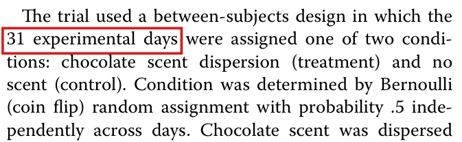(S1) Design. Methods, p. 2 (PDF p. 2): “We conducted a trial over 31 days in an 800-square-foot independent bookstore in Canada.” p. 3 (PDF p. 3), left column: “The trial used a between-subjects design in which the 31 experimental days were assigned one of two conditions: chocolate scent dispersion (treatment) and no scent (control). Condition was determined by Bernoulli (coin flip) random assignment with probability .5 independently across days.” (S2) Outcomes. p. 3 (PDF p. 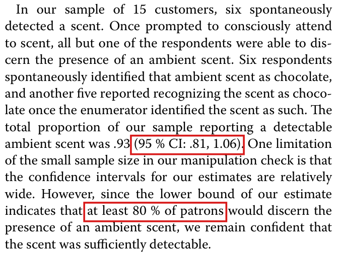3), left column: “Sales data were recorded in three categories: book sales, café sales (pastries, coffee, and tea), and bulk sales (primarily coffee beans, but also loose tea and spices).” (S3) The manipulation check. p. 3 (PDF p. 3), right column, first paragraph of ‘Results and discussion’: “A manipulation check modeled after Doucé et al. was conducted to evaluate four aspects of the scent: spontaneous detection, prompted detection, spontaneous identification, and recognition of the scent. Fifteen customers were asked to respond to questions about the store atmosphere. To assess spontaneous detection, customers were asked whether they noticed something special in the store atmosphere, with responses coded as 1 if the customer mentioned an ambient scent, 0 otherwise. If the customer did not volunteer that a scent was present, ambient scent was mentioned and the subject was asked whether they could detect a scent now that scent was mentioned. Subjects were then asked if they could identify the scent. Subjects who did not spontaneously identify the scent as chocolate were asked if they recognized the scent as chocolate.” Second paragraph, last sentence: “Our objective was to maintain a detectable ambient scent; we did not seek to eliminate spontaneous detection of the chocolate scent.” The third paragraph is the passage of finding P040-E001 and is transcribed in full in P040-T3. The article names no method for its interval, gives no formula for it and describes no sampling scheme for the fifteen customers. (S4) The two regression analyses. p. 3 (PDF p. 3), right column, last lines, continuing on p. 4 (PDF p. 4), left column: “We present two regression-based analyses of the trial. The first is a simple ordinary least squares regression of our four outcomes: total sales, bulk sales, café sales, and book sales in Canadian dollars (CAD). This strategy is logically equivalent to taking a simple mean difference between treatment and control. To improve efficiency, the second strategy uses ordinary least squares adjusting for a mean-centered linear time trend as well as mean-centered fixed effects for the day of week, following Lin (2013). In all cases, robust standard errors are used to estimate standard errors, with $p$ values computed under a normal approximation.” p. 4 (PDF p. 4), right column: “In Table 1, we present our estimates of the control means and average treatment effects of the chocolate scent, as computed with ordinary least squares. The direction of the treatment effect on total sales was positive but not statistically significant. None of our estimates of treatment effects are statistically significant at the two-tailed $p$ < .10 level. Our findings are not substantively altered by adjusting for time trends.” (S5) Table 1, p. 5 (PDF p. 5), as printed. Title: “Table 1 Estimated effects of chocolate scent on bookstore sales”. Columns: “Outcome”, “Unadjusted estimates”, “Adjusted for time trends”. Rows (unadjusted | adjusted). “Total sales”: “Control mean” 575.4 (SE = 34.7) | 593.5 (SE = 30.4); “Treatment effect” 36.6 (SE = 51.6) | 2.7 (SE = 41.7). “Bulk sales”: “Control mean” 72.0 (SE = 13.4) | 71.2 (SE = 16.4); “Treatment effect” 21.8 (SE = 17.5) | 23.2 (SE = 21.2). “Café sales”: “Control mean” 334.7 (SE = 15.2) | 336.5 (SE = 12.6); “Treatment effect” −5.5 (SE = 21.1) | −8.9 (SE = 16.2). “Book sales”: “Control mean” 168.7 (SE = 22.5) | 185.7 (SE = 22.9); “Treatment effect” 20.4 (SE = 32.0) | −11.6 (SE = 32.5). Note under the table: “Estimates of control means and average treatment effects of chocolate scent on total sales, bulk coffee bean/loose tea/spice sales, café sales, and book sales in Canadian dollars. All estimates computed using ordinary least squares regression with robust standard errors. Unadjusted estimates computed without covariates. Adjusted estimates computed using a linear control for the day of experiment and fixed effects for the day of week, all mean-centered”. The table prints no $p$ value; the only $p$ values the article reports are the two of p. 5 (transcribed in P040-T5). 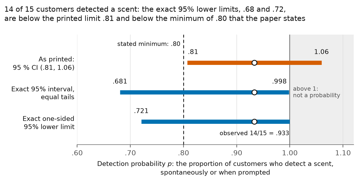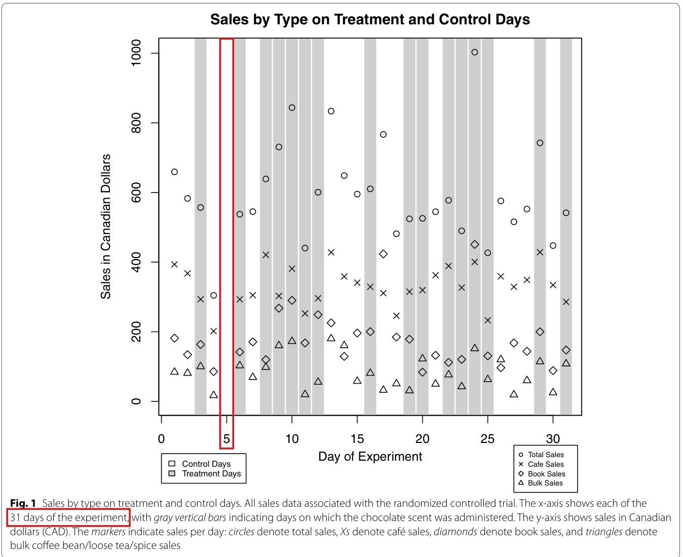(S6) Replication material; this paragraph is read from the deposited files, not from a page of the article. p. 3 (PDF p. 3), left column: “Full replication data and code are available at the Yale Institution for Social and Policy Studies data archive (http://isps.research.yale.edu/research/data).” The staged archive is staged/code/yale-dataverse-KUKU37-v2.0 (a daily-sales CSV, an R script, the manipulation-check Stata file and its label file). (a) The manipulation-check file has 15 rows and four 0/1 variables with sums notice 6, detect 14, identify 6 and recognize 11; every row with notice = 1 has detect = 1. The ‘detectable ambient scent’ of p. 3 is detection spontaneously or after prompting, the variable detect: 14 of 15. The archive has no code for the interval (.81, 1.06). (b) The sales CSV has $N = 30$ rows, one for each of the days $d$ = 1, 2, 3, 4, 6, 7, …, 31 of August (there is no row for day 5), with Treat = 1 on 16 days and Treat = 0 on 14 days; in every row the total equals book + café + bulk. (c) The R script fits, for each of the four outcomes $y$, lm(y ~ Treat) and lm(y ~ Treat + date2 + dowmat), where date2 is the day number minus its mean and dowmat holds the seven indicators of (day number mod 7), each minus its mean. Its helper robust.se multiplies the heteroskedasticity-robust sandwich covariance by (M/(M−1))·((N−1)/(N−K)) with M = N = 30 singleton clusters and K the model rank, which is the factor N/(N−K) (HC1), and passes the result to lmtest::coeftest without a df argument; coeftest then takes the model's residual degrees of freedom and returns Student-$t$ $p$ values (df = Inf would give normal ones). (d) The rows, as ‘day: Treat, book sales, café sales, bulk sales, total sales’ in CAD (columns Treat, Book Tot., cafee, Beans, Grand Tot. of the CSV; every entry is an exact decimal): 1: 0, 181.71, 393.52, 84.2, 659.43; 2: 0, 134.35, 367.57, 81.15, 583.07; 3: 1, 163.55, 293.35, 100.05, 556.95; 4: 0, 85.65, 201.92, 17.05, 304.62; 6: 1, 141.9, 293.21, 102.71, 537.82; 7: 0, 171, 305.03, 69.19, 545.22; 8: 1, 119.9, 420.96, 98.15, 639.01; 9: 1, 267.6, 302.88, 160.35, 730.83; 10: 1, 290.15, 381.19, 172.51, 843.85; 11: 1, 168, 252.55, 19.8, 440.35; 12: 1, 249.05, 296.13, 55.49, 600.67; 13: 0, 225.55, 427.95, 180.31, 833.81; 14: 0, 129.3, 358.84, 160.32, 648.46; 15: 0, 196.4, 341.07, 57.98, 595.45; 16: 1, 200.25, 329.18, 81.02, 610.45; 17: 0, 423.56, 310.92, 32.35, 766.83; 18: 0, 184.75, 246.09, 50.82, 481.66; 19: 1, 178.65, 314.99, 30.8, 524.44; 20: 1, 83.9, 319.55, 122.36, 525.81; 21: 0, 132.35, 362.47, 49.88, 544.7; 22: 1, 112.05, 389, 76.62, 577.67; 23: 1, 120.65, 326.86, 42.45, 489.96; 24: 1, 450.95, 400.49, 151.7, 1003.14; 25: 1, 130.75, 233, 63.05, 426.8; 26: 0, 96.75, 359, 120.13, 575.88; 27: 0, 167.9, 329, 19.05, 515.95; 28: 0, 143.8, 349, 59.91, 552.71; 29: 1, 200, 428.44, 114.12, 742.56; 30: 0, 88.6, 334.07, 24.97, 447.64; 31: 1, 147.6, 286, 108.12, 541.72. (S7) Audit notation; not in the paper (from the validators' derivations). Binomial model: $n = 15$; for $p \in [0,1]$ and $E \subseteq \{0,\dots,15\}$, $P_p(E) = \sum_{k \in E} \binom{15}{k} p^k (1-p)^{15-k}$ is the law of the number $X$ of customers who detect a scent when the fifteen responses are independent with a common detection probability $p$; the observed count is $x = 14$. Regression: rows $i = 1,\dots,30$ of the table in (S6)(d), with day $d_i$, assignment $T_i \in \{0,1\}$ and outcome $y_i$ (one of total, bulk, café, book); $N = 30$; $\bar d = \tfrac{1}{30}\sum_i d_i = 491/30$; for $c \in \{0,\dots,6\}$, $n_c = \#\{i : d_i \bmod 7 = c\}$, so $(n_0,\dots,n_6) = (4,5,5,5,4,3,4)$. The unadjusted design $X^{u}$ is the $30 \times 2$ matrix with rows $(1,\ T_i)$. The adjusted design $X^{a}$ is the $30 \times 9$ matrix with rows $\bigl(1,\ T_i,\ d_i - \bar d,\ \mathbf{1}\{d_i \bmod 7 = c\} - n_c/30 \ (c = 0,\dots,5)\bigr)$. (The script's design has a tenth column, the centred indicator of $d \bmod 7 = 6$; the seven centred indicators sum to zero in every row, the ten columns have rank 9 and the same column space as $X^{a}$, and R drops the aliased column. The coefficient on $T$ and its robust variance depend on the other columns only through their span.) For a design $X$ of full column rank $K$ and an outcome $y$: $G = (X^\top X)^{-1}X^\top$, $\hat\beta = Gy$, $e = y - X\hat\beta$, $\hat\beta_T$ is the second coordinate of $\hat\beta$ (the coefficient on $T$), $$v = \frac{N}{N-K}\sum_{i=1}^{N} (G_{2i}\,e_i)^2$$ is the $(2,2)$ entry of the HC1 covariance $\frac{N}{N-K}(X^\top X)^{-1}\bigl(\sum_i e_i^2 x_i x_i^\top\bigr)(X^\top X)^{-1}$ ($x_i^\top$ the $i$-th row of $X$), $q = \hat\beta_T^2/v$ is the squared robust $t$ statistic and $\nu = N - K$ is the residual degrees of freedom (28 for $X^{u}$, 21 for $X^{a}$). Reference distributions: $\Phi$ is the standard normal distribution function and $$p_N(q) = 2\bigl(1 - \Phi(\sqrt q)\bigr) = 1 - \sqrt{2/\pi}\int_0^{\sqrt q} e^{-u^2/2}\,du;$$ for $\nu > 0$, $f_\nu(t) = \frac{\Gamma((\nu+1)/2)}{\sqrt{\nu\pi}\,\Gamma(\nu/2)}\,(1 + t^2/\nu)^{-(\nu+1)/2}$ is the Student-$t$ density with $\nu$ degrees of freedom and $$p_T(q;\nu) = 1 - 2\int_0^{\sqrt q} f_\nu(t)\,dt.$$ Rounding: a real $x$ rounds to the two-decimal number $w$ when $w - \tfrac{1}{200} \le x < w + \tfrac{1}{200}$. Scope of the list. Four candidates are rated errors (ratings.json): P040-E001 (Moderate), P040-E002, P040-E003 and P040-N008 (Minor). Two of them correct mathematical content and are targets: P040-E001 (the interval (.81, 1.06) is used as a 95% lower bound of 80% that it cannot support: counterexample P040-T1, corrected statement P040-T2, passage as printed P040-T3) and P040-E003 (the two printed $p$ values are Student-$t$ values, not the normal-approximation values the Methods name: counterexample P040-T4, corrected statement P040-T5). P040-E002 (31 experimental days against the 30 analysed daily observations) is a finding about data and reporting whose repair is a clarification, and P040-N008 is bibliographic; neither is a target (see error_findings_not_targeted). P040-N001, N002, N006 and N007 are not confirmed, P040-N003, N004 and N005 are undetermined and P040-N009 is out of scope. None of the seven headline claims (candidates.json, P040-H1 to P040-H7) is a mathematical statement: they are empirical estimates, a description of the design and interpretive remarks, so there is no headline_result target; P040-H6 is the claim touched by P040-E001 and P040-H2 the claim touched by P040-E003.

Effective claim (source TeX): An exact witness (validator's construction; not in the paper). Grant the favourable model in which the fifteen responses are independent with a common detection probability $p$. At $p = 4/5$, a value excluded by the printed nominal interval, no deterministic interval rule based on the count that excludes $4/5$ at the observed count can cover with probability $.95$, and the rule that reproduces the printed numbers covers with probability about $.815$. Setting. $n = 15$; $P_p(X = k) = \binom{15}{k} p^k (1-p)^{15-k}$ for $k = 0,\dots,15$ (standing assumption (S7)); observed count $x = 14$; witness $p_0 = 4/5$. (A1) $$P_{4/5}(X = 14) = 15\,(4/5)^{14}(1/5) = \frac{3 \cdot 4^{14}}{5^{14}} = \frac{805306368}{6103515625} = 0.13194139533312 > \frac{1}{20}.$$ (A2) Method-free bound. For every map $I$ from $\{0,\dots,15\}$ to subsets of $\mathbb{R}$ with $4/5 \notin I(14)$, $$P_{4/5}\bigl(4/5 \in I(X)\bigr) \le 1 - P_{4/5}(X = 14) = \frac{5298209257}{6103515625} = 0.86805860466688 < \frac{19}{20}.$$ The printed interval $(.81,\ 1.06)$ excludes $4/5$, and so does every interval whose lower endpoint rounds to $.81$ (such an endpoint is at least $.805 > 4/5$). In the same way, for every map $\ell : \{0,\dots,15\} \to \mathbb{R}$ with $\ell(14) > 4/5$, $P_{4/5}\bigl(\ell(X) \le 4/5\bigr) \le \frac{5298209257}{6103515625} < \frac{19}{20}$. (A3) The rule that reproduces the print. For $k = 0,\dots,15$ put $c_k = k/15$, $r_k = \tfrac{49}{25}\sqrt{c_k(1-c_k)/15}$ and $I_W(k) = [\,c_k - r_k,\ c_k + r_k\,]$ (the plug-in normal, or Wald, interval with $z = 1.96 = 49/25$). Then: (a) $c_{14} = 14/15$, $c_{14}(1-c_{14})/15 = 14/3375$, $r_{14}^2 = 33614/2109375$, and $$0.8070 < c_{14} - r_{14} < 0.8071, \qquad 1.0595 < c_{14} + r_{14} < 1.0596,$$ so $I_W(14)$ rounds to the printed $(.81,\ 1.06)$, its upper endpoint exceeds $1$, and $4/5 \notin I_W(14)$. (b) $4/5 \in I_W(k)$ if and only if $k \in \{9,10,11,12,13\}$ (equivalently $(4/5 - c_k)^2 \le r_k^2$, a comparison of rationals). (c) $$P_{4/5}\bigl(4/5 \in I_W(X)\bigr) = \sum_{k=9}^{13}\binom{15}{k}(4/5)^k(1/5)^{15-k} = \frac{24866193408}{30517578125} = 0.814815425593344 < \frac{19}{20}.$$ (d) $c_k - r_k \le 4/5$ if and only if $k \le 13$, and $$P_{4/5}\bigl(c_X - r_X \le 4/5\bigr) = 1 - P_{4/5}(X \ge 14) = 1 - \frac{19 \cdot 4^{14}}{5^{15}} = 1 - \frac{5100273664}{30517578125} = \frac{25417304461}{30517578125} = 0.832874232578048 < \frac{19}{20}.$$ (A4) Robustness to the multiplier. (b), (c) and (d) hold unchanged when $49/25$ is replaced by any real $z$ with $19599/10000 \le z \le 19601/10000$; this range contains the normal $.975$ quantile $1.95996\ldots$ Consequence. Under the binomial model the endpoint $.81$ is not a lower confidence bound with confidence $.95$ (nor with confidence $.975$, the one-sided level of an equal-tailed 95% interval): when the true detection probability is exactly $.80$, the rule that produced it puts its lower endpoint above $.80$ with probability $\frac{5100273664}{30517578125} = 0.167125767421952$, and the count $14$ alone, which forces the exclusion of $.80$, has probability $0.13194139533312$. So ‘at least 80 % of patrons’ does not follow at the stated confidence from 14 detections in 15.

: SAP.P040.T1WholeStatement

Theorem: SAP.P040.T1

Statement hash: a5cb98f162205151bea4a330cf794076540cbea7c32d4658dadc5603bd37a59d

Statement definition: SAP.P040.T1WholeStatement

Certificate. 20261104T160517Z

Declaration review: faithful; 2026-11-04T16:25:53Z; binding v2

Evidence scope: Certification checks formal proof objects. Statement fidelity is a model judgment. Author review is separate.

Proof dependencies: Independently extracted

Manifest annotation reconciliation: Effective use follows the source-bound dependency observation; original annotations are retained in the crosswalk.

AronowAudit.P040.binomialMass_nonneg: observed used

AronowAudit.P040.binomialMass_total: observed used

AronowAudit.P040.exclude_observed_count_bound: observed used

Source and evidence metadata · sap-2026-11-08-assured-release

P040-T3

Results and discussion, third paragraph (the manipulation-check estimate, its interval and the inference ‘at least 80 % of patrons’); as printed

p. 3 (PDF p. 3; headed ‘Page 3 of 6’), right column, paragraph beginning ‘In our sample of 15 customers’

p. 3, right column, paragraph beginning "In our sample of 15 customers" (PDF p. 3). The observed proportion rounds to .93 and the reconstructed Wald endpoints round to .81 and 1.06 with the stated brackets and an upper endpoint above one. This states the canonical passage's retained mathematical content P1 and P2; the customer counts are inputs and no exact coverage claim is attributed to it.

Historical component credits

Proved AronowAudit.P040.printed_wald_arithmetic Historical support retained; baseline fidelity: ok; manifest: used; used in Solution; The assigned component is P2, equivalently T1 A3(a), so the absence of a .93-rounding conclusion does not narrow this row; it is a separate target-coverage omission.

Formal result: whole

Formal statement · Proof · Definitions

Assumptions and verification

Claim revision: catalog:88a5642a1cabbd4c888f1cdc33ba131266e7db5bf9ee1e329f51f3c71a80d6c2

Effective claim (source TeX): As printed. “In our sample of 15 customers, six spontaneously detected a scent. Once prompted to consciously attend to scent, all but one of the respondents were able to discern the presence of an ambient scent. Six respondents spontaneously identified that ambient scent as chocolate, and another five reported recognizing the scent as chocolate once the enumerator identified the scent as such. The total proportion of our sample reporting a detectable ambient scent was .93 (95 % CI: .81, 1.06). One limitation of the small sample size in our manipulation check is that the confidence intervals for our estimates are relatively wide. However, since the lower bound of our estimate indicates that at least 80 % of patrons would discern the presence of an ambient scent, we remain confident that the scent was sufficiently detectable.” Formalizable content of the passage, in the notation of (S7) and P040-T1. (P1) The estimate: $14/15 = 0.9333\ldots$ rounds to the printed $.93$. (P2) The interval: the paper gives no formula; the plug-in normal interval $I_W(14) = 14/15 \pm \tfrac{49}{25}\sqrt{14/3375}$ has $0.8070 < 14/15 - \tfrac{49}{25}\sqrt{14/3375} < 0.8071$ and $1.0595 < 14/15 + \tfrac{49}{25}\sqrt{14/3375} < 1.0596$, so it rounds to the printed $(.81,\ 1.06)$; its upper endpoint exceeds $1$. (P1) and (P2) are correct arithmetic. The quoted estimate and reconstructed Wald arithmetic are retained. The lower endpoint has the conventional approximate confidence interpretation; the article does not claim uniform exact finite-sample .95 coverage. The historical exact-coverage proposition and its negation are auxiliary calibration objects under T1, not attributed printed content.

: SAP.P040.T3Statement

Theorem: SAP.P040.T3

Statement hash: d21ef8f3faca6ceaecb79d710422d4941a11c701eeaac9fc587a1a6052de07f7

Statement definition: SAP.P040.T3Statement

Certificate. 20261104T160517Z

Declaration review: faithful; 2026-11-04T16:25:53Z; binding v2

Evidence scope: Certification checks formal proof objects. Statement fidelity is a model judgment. Author review is separate.

Proof dependencies: Independently extracted

Source and evidence metadata · sap-2026-11-08-assured-release

P040-T2

Results and discussion, manipulation check: ‘.93 (95 % CI: .81, 1.06)’ and ‘at least 80 % of patrons’, as repaired by Sol: the exact binomial 95% interval for 14 detections in 15, which contains .80

p. 3 (PDF p. 3; headed ‘Page 3 of 6’), right column, paragraph beginning ‘In our sample of 15 customers’

p. 3, right column, manipulation check (PDF p. 3), corrected. Under the independent common-probability binomial model, the exact equal-tailed and one-sided intervals have the stated unique endpoints, rounding, inclusion of .80, and uniform coverage of at least 95%, while excluding .80 at count 14 prevents that coverage guarantee.

Historical component credits

Proved AronowAudit.P040.observed_proportion_rounds Historical support retained; baseline fidelity: ok; manifest: used; used in Solution; The exact proportion 14/15 rounds to .93 under precisely the claim's stated rounding convention.
Proved AronowAudit.P040.observed_tail_identities Historical support retained; baseline fidelity: ok; manifest: used; used in Solution; The exact binomial-tail polynomial identities hold for all real p, extending the claim's [0,1] identities without altering their probability-domain meaning.
Proved AronowAudit.P040.observedUpper_continuous Historical support retained; baseline fidelity: ok; manifest: used; used in Solution; Global continuity of the observed-tail polynomial strengthens its required continuity on [0,1] and specializes to the claim unchanged.
Proved AronowAudit.P040.observedUpper_hasDerivAt Historical support retained; baseline fidelity: ok; manifest: used; used in Solution; The derivative formula holds at every real argument, strengthening its required validity on the probability interval without changing the formula.
Proved AronowAudit.P040.observedUpper_strictMono Historical support retained; baseline fidelity: ok; manifest: used; used in Solution; Strict increase of the observed upper-tail polynomial on the closed interval [0,1] is the monotonicity required in component (ii), including endpoints.
Proved AronowAudit.P040.observedLower_strictAnti Historical support retained; baseline fidelity: ok; manifest: used; used in Solution; Strict decrease of 1-p^15 on the entire closed parameter interval is exactly the lower-tail monotonicity in component (ii), using the separate tail identity.
Proved AronowAudit.P040.countProbability_mono Historical support retained; baseline fidelity: ok; manifest: used; used in Solution; The selected aggregate row exports the required component; this supporting certificate is not separately invoked.
Proved AronowAudit.P040.countProbability_complement Historical support retained; baseline fidelity: ok; manifest: used; used in Solution; The selected aggregate row exports the required component; this supporting certificate is not separately invoked.
Proved AronowAudit.P040.countProbability_union_le Historical support retained; baseline fidelity: ok; manifest: used; used in Solution; The selected aggregate row exports the required component; this supporting certificate is not separately invoked.
Proved AronowAudit.P040.upper_tail_rejection_le Historical support retained; baseline fidelity: ok; manifest: used; used in Solution; The selected aggregate row exports the required component; this supporting certificate is not separately invoked.
Proved AronowAudit.P040.lower_tail_rejection_le Historical support retained; baseline fidelity: ok; manifest: used; used in Solution; The selected aggregate row exports the required component; this supporting certificate is not separately invoked.
Proved AronowAudit.P040.exact_binomial_coverage Historical support retained; baseline fidelity: ok; manifest: used; used in Solution; Both tail-inverted sets have coverage at least 19/20 for every p in [0,1], exactly as required by component (vi), including boundary parameters. The binomial model is expressly part of the corrected target; it is not supplied by random assignment of experimental days. The supplied public description accurately reports this result.
Proved AronowAudit.P040.exact_endpoint_sign_certificates Historical support retained; baseline fidelity: ok; manifest: used; used in Solution; The exported endpoint theorem already supplies the actual roots and their brackets.
Proved AronowAudit.P040.exact_interval_contains_eighty_percent Historical support retained; baseline fidelity: ok; manifest: used; used in Solution; The two exact tail probabilities and inclusion of 4/5 in both corrected confidence sets agree with component (v).
Proved AronowAudit.P040.unique_bracketed_root Historical support retained; baseline fidelity: ok; manifest: used; used in Solution; Root existence and uniqueness are already exported by corrected_binomial_endpoints.
Proved AronowAudit.P040.corrected_binomial_endpoints Historical support retained; baseline fidelity: ok; manifest: used; used in Solution; The statement exports all three actual endpoint roots, their uniqueness on [0,1], the required brackets and closed-set identities, and the stated two-decimal rounding. The binomial model is expressly part of the corrected target; it is not supplied by random assignment of experimental days. The supplied public description accurately reports this result.
Proved AronowAudit.P040.observed_upper_boundary_values Historical support retained; baseline fidelity: ok; manifest: used; used in Solution; The statement gives precisely the two observed upper-tail boundary evaluations required in component (ii).
Proved AronowAudit.P040.corrected_six_decimal_rounding Historical support retained; baseline fidelity: ok; manifest: used; used in Solution; The endpoint membership and root-equation hypotheses identify exactly the roots in the claim, and the conclusion gives their correct six-decimal rounding cells.

Formal result: whole

Formal statement · Proof · Definitions

Assumptions and verification

Claim revision: catalog:35e0864ddb62b45a849dbad5723d5c999f0229758829789fab642c9440258bd2

Effective claim (source TeX): [Corrected; Sol's smallest_repair, validated.json, P040-E001, verbatim] “Keep the observed 14 of 15 detections; condition inference on an independent common-probability binomial sampling model, replace the nominal interval with the exact equal-tailed 95% interval [.680515, .998314] (or [.68, 1.00] at the printed precision), and replace the minimum-80%-of-patrons assertion with a statement about the high observed detection rate and its substantial uncertainty. Generalization to patrons requires appropriate sampling assumptions.” Corrected text (validated.json, prior_correction.corrected_text, status ‘correct’), verbatim: “Fourteen of the fifteen surveyed customers reported detecting an ambient scent, either spontaneously or after prompting. Under an independent common-probability binomial sampling model, the exact equal-tailed 95% confidence interval is [.680515, .998314]. The observed detection rate was high, but the small sample does not support a 95% confidence-based lower bound of 80% for patrons; generalization beyond the surveyed customers requires appropriate sampling assumptions.” [Mathematical content, with every hypothesis] Hypothesis (H): the fifteen responses are independent and each customer detects a scent with the same unknown probability $p \in [0,1]$, so that the number $X$ of detections has the law $P_p$ of (S7), $P_p(X = k) = \binom{15}{k}p^k(1-p)^{15-k}$. The observed count is $x = 14$. Definitions: for $k \in \{0,\dots,15\}$ and $p \in [0,1]$ put $$S_k(p) = P_p(X \ge k), \qquad F_k(p) = P_p(X \le k),$$ $$C(k) = \{p \in [0,1] : S_k(p) \ge \tfrac{1}{40} \text{ and } F_k(p) \ge \tfrac{1}{40}\}, \qquad C^{+}(k) = \{p \in [0,1] : S_k(p) \ge \tfrac{1}{20}\}.$$ $C(k)$ is the exact (Clopper–Pearson) equal-tailed 95% confidence set obtained by inverting the two binomial tail tests, and $C^{+}(k)$ is the exact one-sided 95% lower confidence set. (i) Point estimate. $14/15 = 0.9333\ldots$ rounds to the printed $.93$. (ii) Tail functions at the observed count. For $p \in [0,1]$: $S_{14}(p) = 15p^{14}(1-p) + p^{15} = p^{14}(15 - 14p)$ and $F_{14}(p) = 1 - p^{15}$. $S_{14}$ is continuous and strictly increasing on $[0,1]$ with $S_{14}(0) = 0$ and $S_{14}(1) = 1$ (its derivative is $210\,p^{13}(1-p) > 0$ on $(0,1)$); $F_{14}$ is strictly decreasing on $[0,1]$. (iii) The interval. There are unique $L, L_{\mathrm{one}} \in (0,1)$ with $S_{14}(L) = 1/40$ and $S_{14}(L_{\mathrm{one}}) = 1/20$, and $U = (39/40)^{1/15}$ is the unique $p \in [0,1]$ with $F_{14}(p) = 1/40$. Then $$C(14) = [L,\ U], \qquad C^{+}(14) = [L_{\mathrm{one}},\ 1].$$ (iv) Numerical values. $$0.680515 < L < 0.680516, \qquad 0.998313 < U < 0.998314, \qquad 0.720603 < L_{\mathrm{one}} < 0.720604;$$ equivalently $S_{14}(680515/10^6) < \tfrac{1}{40} < S_{14}(680516/10^6)$, $(998313/10^6)^{15} < \tfrac{39}{40} < (998314/10^6)^{15}$ and $S_{14}(720603/10^6) < \tfrac{1}{20} < S_{14}(720604/10^6)$. To six decimals the interval is $[.680515,\ .998314]$; at the paper's two-decimal precision it is $[.68,\ 1.00]$, against the printed $(.81,\ 1.06)$. (v) The threshold of 80% is not excluded. $$S_{14}(4/5) = \frac{19 \cdot 4^{14}}{5^{15}} = \frac{5100273664}{30517578125} = 0.167125767421952 > \frac{1}{20} > \frac{1}{40}, \qquad F_{14}(4/5) = 1 - (4/5)^{15} = \frac{29443836301}{30517578125} \ge \frac{1}{40}.$$ Hence $4/5 \in C(14)$ and $4/5 \in C^{+}(14)$, that is, $L < L_{\mathrm{one}} < 4/5$: neither the equal-tailed exact 95% interval nor the one-sided exact 95% lower bound supports $p \ge .80$, and the exact one-sided test of $p \le 4/5$ against $p > 4/5$ at the count 14 has $p$ value $0.167125767421952$. (vi) What makes ‘95%’ true of the replacement. Under (H), for every $p \in [0,1]$, $$P_p\bigl(p \in C(X)\bigr) \ge \frac{19}{20} \qquad\text{and}\qquad P_p\bigl(p \in C^{+}(X)\bigr) \ge \frac{19}{20}.$$ (For fixed $p$, the set $\{k : S_k(p) < 1/40\}$ is an upper set of counts and has $P_p$-probability below $1/40$; the set $\{k : F_k(p) < 1/40\}$ is a lower set of counts and has $P_p$-probability below $1/40$; likewise with $1/20$ for $C^{+}$.) By P040-T1 (A2) no deterministic count-based rule that excludes $4/5$ at $k = 14$ has this property. What the corrected statement does not assert: that the detection probability is below $.80$, that the scent was not detectable, or anything about patrons beyond the fifteen surveyed customers without a sampling assumption that makes (H) describe them.

: SAP.P040.T2Statement

Theorem: SAP.P040.T2

Statement hash: b616d7628d28ee7bceaef457ba227b5b66ae1ee0bf2053f8b63ab172200fbe64

Statement definition: SAP.P040.T2Statement

Certificate. 20261104T160517Z

Declaration review: faithful; 2026-11-04T16:25:53Z; binding v2

Evidence scope: Certification checks formal proof objects. Statement fidelity is a model judgment. Author review is separate.

Proof dependencies: Independently extracted

Manifest annotation reconciliation: Effective use follows the source-bound dependency observation; original annotations are retained in the crosswalk.

AronowAudit.P040.countProbability_complement: observed used

AronowAudit.P040.countProbability_mono: observed used

AronowAudit.P040.countProbability_union_le: observed used

AronowAudit.P040.exact_endpoint_sign_certificates: observed used

AronowAudit.P040.lower_tail_rejection_le: observed used

AronowAudit.P040.unique_bracketed_root: observed used

AronowAudit.P040.upper_tail_rejection_le: observed used

Source and evidence metadata · sap-2026-11-08-assured-release

P040-T4

Methods, ‘with p values computed under a normal approximation’, against the two p values printed in the Results (café sales, two-tailed p = .59; bulk sales, two-tailed p = .29); the witness is the exact recalculation of the two adjusted regressions from the deposited data and is not in the paper

p. 4 (PDF p. 4; headed ‘Page 4 of 6’), left column, first paragraph, last sentence; p. 5 (PDF p. 5; headed ‘Page 5 of 6’), left column, last paragraph; Table 1, p. 5 (PDF p. 5)

p. 4, left column, Methods, and p. 5, left column, last paragraph (PDF pp. 4-5); Table 1, p. 5. The actual adjusted cafe and bulk regressions have the stated exact coefficients, HC1 variances, statistics and decimal rounding; their normal-reference p values round to .58 and .28, whereas the printed .59 and .29 use the Student-t reference.

Historical component credits

Proved AronowAudit.P040.regression_witness_arithmetic Historical support retained; baseline fidelity: ok; manifest: used; used in Solution; Fidelity sweep: ok
Proved AronowAudit.P040.normal_polynomial_integral Historical support retained; baseline fidelity: ok; manifest: used; used in Solution; The selected aggregate row exports the required component; this supporting certificate is not separately invoked.
Proved AronowAudit.P040.normal_kernel_error Historical support retained; baseline fidelity: ok; manifest: used; used in Solution; The selected aggregate row exports the required component; this supporting certificate is not separately invoked.
Proved AronowAudit.P040.normal_integral_enclosure Historical support retained; baseline fidelity: ok; manifest: used; used in Solution; The selected aggregate row exports the required component; this supporting certificate is not separately invoked.
Proved AronowAudit.P040.normal_p_enclosure Historical support retained; baseline fidelity: ok; manifest: used; used in Solution; The selected aggregate row exports the required component; this supporting certificate is not separately invoked.
Proved AronowAudit.P040.normal_decimal_certificate Historical support retained; baseline fidelity: ok; manifest: used; used in Solution; The selected aggregate row exports the required component; this supporting certificate is not separately invoked.
Counterexample proved AronowAudit.P040.normal_reference_counterexample_bounds Historical support retained; baseline fidelity: ok; manifest: used; used in Solution; A numerical component of the counterexample, not a standalone regression identification; R235-04 supplies that separate component. The supplied target fixes the normal-reference convention, so no additional paper search was needed.
Counterexample proved AronowAudit.P040.normal_reference_rounding_mismatch Historical support retained; baseline fidelity: ok; manifest: used; used in Solution; recorded_normal_counterexample states the mismatch directly on the actual fitted statistics.
Proved AronowAudit.P040.unadjusted_gram_certificate Withdrawn support; baseline fidelity: wrong_credit; manifest: used; used in Solution; Wrong credit for T4: this row concerns the unadjusted design, whereas both T4 witnesses use the adjusted design.
Proved AronowAudit.P040.unadjusted_inverse_product_certificate Withdrawn support; baseline fidelity: wrong_credit; manifest: used; used in Solution; Wrong credit for T4: this row concerns the unadjusted design, whereas both T4 witnesses use the adjusted design.
Proved AronowAudit.P040.unadjusted_gram_inverse Withdrawn support; baseline fidelity: wrong_credit; manifest: used; used in Solution; Wrong credit for T4: this row concerns the unadjusted design, whereas both T4 witnesses use the adjusted design.
Proved AronowAudit.P040.unadjusted_crossproduct_certificate Withdrawn support; baseline fidelity: wrong_credit; manifest: used; used in Solution; Wrong credit for T4: this row concerns the unadjusted design, whereas both T4 witnesses use the adjusted design.
Proved AronowAudit.P040.unadjusted_coefficients_certificate Withdrawn support; baseline fidelity: wrong_credit; manifest: used; used in Solution; Wrong credit for T4: this row concerns the unadjusted design, whereas both T4 witnesses use the adjusted design.
Proved AronowAudit.P040.unadjusted_treatment_weights_certificate Withdrawn support; baseline fidelity: wrong_credit; manifest: used; used in Solution; Wrong credit for T4: this row concerns the unadjusted design, whereas both T4 witnesses use the adjusted design.
Proved AronowAudit.P040.unadjusted_residuals_certificate Withdrawn support; baseline fidelity: wrong_credit; manifest: used; used in Solution; Wrong credit for T4: this row concerns the unadjusted design, whereas both T4 witnesses use the adjusted design.
Proved AronowAudit.P040.unadjusted_hc1_variance_certificate Withdrawn support; baseline fidelity: wrong_credit; manifest: used; used in Solution; Wrong credit for T4: this row concerns the unadjusted design, whereas both T4 witnesses use the adjusted design.
Proved AronowAudit.P040.unadjusted_squared_statistics_certificate Withdrawn support; baseline fidelity: wrong_credit; manifest: used; used in Solution; Wrong credit for T4: this row concerns the unadjusted design, whereas both T4 witnesses use the adjusted design.
Proved AronowAudit.P040.adjusted_gram_certificate Historical support retained; baseline fidelity: ok; manifest: used; used in Solution; The selected aggregate row exports the required component; this supporting certificate is not separately invoked.
Proved AronowAudit.P040.adjusted_inverse_product_certificate Historical support retained; baseline fidelity: ok; manifest: used; used in Solution; The selected aggregate row exports the required component; this supporting certificate is not separately invoked.
Proved AronowAudit.P040.adjusted_gram_inverse Historical support retained; baseline fidelity: ok; manifest: used; used in Solution; The selected aggregate row exports the required component; this supporting certificate is not separately invoked.
Proved AronowAudit.P040.adjusted_crossproduct_certificate Historical support retained; baseline fidelity: ok; manifest: used; used in Solution; The selected aggregate row exports the required component; this supporting certificate is not separately invoked.
Proved AronowAudit.P040.adjusted_coefficients_certificate Historical support retained; baseline fidelity: ok; manifest: used; used in Solution; The selected aggregate row exports the required component; this supporting certificate is not separately invoked.
Proved AronowAudit.P040.adjusted_treatment_weights_certificate Historical support retained; baseline fidelity: ok; manifest: used; used in Solution; The selected aggregate row exports the required component; this supporting certificate is not separately invoked.
Proved AronowAudit.P040.adjusted_residuals_certificate Historical support retained; baseline fidelity: ok; manifest: used; used in Solution; The selected aggregate row exports the required component; this supporting certificate is not separately invoked.
Proved AronowAudit.P040.adjusted_hc1_variance_certificate Historical support retained; baseline fidelity: ok; manifest: used; used in Solution; The selected aggregate row exports the required component; this supporting certificate is not separately invoked.
Proved AronowAudit.P040.adjusted_squared_statistics_certificate Historical support retained; baseline fidelity: ok; manifest: used; used in Solution; The selected aggregate row exports the required component; this supporting certificate is not separately invoked.
Proved AronowAudit.P040.recorded_regression_identification Historical support retained; baseline fidelity: ok; manifest: used; used in Solution; The adjusted cafe/bulk conjuncts cover T4(B1–B2); the all-eight-statistics conjuncts are additional conclusions and do not turn the unadjusted-only rows into components of T4.
Proved AronowAudit.P040.normal_reference_antitone Historical support retained; baseline fidelity: ok; manifest: not used; not used in Solution; The selected aggregate row exports the required component; this supporting certificate is not separately invoked.
Counterexample proved AronowAudit.P040.recorded_normal_counterexample Historical support retained; baseline fidelity: ok; manifest: used; used in Solution; Fidelity sweep: ok
Proved AronowAudit.P040.recorded_table_cells_round Historical support retained; baseline fidelity: ok; manifest: used; used in Solution; Fidelity sweep: ok

Formal result: whole

Formal statement · Proof · Definitions

Assumptions and verification

Claim revision: catalog:c77ec4beea026ae72d77cbc405d6b199d0716b7c3bf1e2287dc8468dbe5d5bda

Effective claim (source TeX): An exact witness (validator's recalculation from the deposited data; not in the paper): for the two regressions whose $p$ values the article prints, the normal-approximation $p$ value named in the Methods does not round to the printed number. Setting. Notation of standing assumption (S7); the 30 rows of (S6)(d); the adjusted design $X^{a}$ ($N = 30$, $K = 9$, $\nu = 21$); $p_N(q) = 2(1 - \Phi(\sqrt q))$. (B1) Café sales (outcome: the café column). $$\hat\beta_T = -\frac{146561}{16484}, \qquad v = \frac{42131842162249950707521}{161509653387533360000}, \qquad q_{\text{café}} = \frac{\hat\beta_T^2}{v} = \frac{12767624825803755635000}{42131842162249950707521}.$$ In decimals $\hat\beta_T \approx -8.891107$ and $\sqrt v \approx 16.151244$, which round to the entries $-8.9$ (SE = 16.2) of Table 1; $q_{\text{café}} \approx 0.303040$, $\sqrt{q_{\text{café}}} \approx 0.550491$. (B2) Bulk sales (outcome: the bulk column). $$\hat\beta_T = \frac{955199}{41210}, \qquad v = \frac{10415886991743115636339}{23072807626790480000}, \qquad q_{\text{bulk}} = \frac{\hat\beta_T^2}{v} = \frac{12396039010057804992800}{10415886991743115636339}.$$ In decimals $\hat\beta_T \approx 23.178816$ and $\sqrt v \approx 21.247014$, which round to the entries $23.2$ (SE = 21.2) of Table 1; $q_{\text{bulk}} \approx 1.190109$, $\sqrt{q_{\text{bulk}}} \approx 1.090921$. (B3) $0.58198 < p_N(q_{\text{café}}) < 0.58199$. This lies strictly inside $(0.575,\ 0.585)$, so the normal-approximation $p$ value rounds to $.58$ and not to the printed $.59$. (B4) $0.27530 < p_N(q_{\text{bulk}}) < 0.27531$. This lies strictly inside $(0.275,\ 0.285)$, so the normal-approximation $p$ value rounds to $.28$ and not to the printed $.29$. Consequence. The sentence ‘with $p$ values computed under a normal approximation’ is false of both $p$ values that the article prints: neither $.59$ nor $.29$ is the two-decimal rounding of $2(1 - \Phi(|\hat\beta_T|/\sqrt v))$ for the regression it is attached to. (They are the Student-$t$ values with 21 degrees of freedom: P040-T5.)

: SAP.P040.T4Statement

Theorem: SAP.P040.T4

Statement hash: ed712692edabe071cd839c854115f23abc405cb833ac71234c37db61bea71d8a

Statement definition: SAP.P040.T4Statement

Certificate. 20261104T160517Z

Declaration review: faithful; 2026-11-04T16:25:53Z; binding v2

Evidence scope: Certification checks formal proof objects. Statement fidelity is a model judgment. Author review is separate.

Proof dependencies: Independently extracted

Manifest annotation reconciliation: Effective use follows the source-bound dependency observation; original annotations are retained in the crosswalk.

AronowAudit.P040.adjusted_coefficients_certificate: observed used

AronowAudit.P040.adjusted_crossproduct_certificate: observed used

AronowAudit.P040.adjusted_gram_certificate: observed used

AronowAudit.P040.adjusted_gram_inverse: observed used

AronowAudit.P040.adjusted_hc1_variance_certificate: observed used

AronowAudit.P040.adjusted_inverse_product_certificate: observed used

AronowAudit.P040.adjusted_residuals_certificate: observed used

AronowAudit.P040.adjusted_squared_statistics_certificate: observed used

AronowAudit.P040.adjusted_treatment_weights_certificate: observed used

AronowAudit.P040.normal_decimal_certificate: observed used

AronowAudit.P040.normal_integral_enclosure: observed used

AronowAudit.P040.normal_kernel_error: observed used

AronowAudit.P040.normal_p_enclosure: observed used

AronowAudit.P040.normal_polynomial_integral: observed used

AronowAudit.P040.normal_reference_rounding_mismatch: observed used

AronowAudit.P040.unadjusted_coefficients_certificate: observed used

AronowAudit.P040.unadjusted_crossproduct_certificate: observed used

AronowAudit.P040.unadjusted_gram_certificate: observed used

AronowAudit.P040.unadjusted_gram_inverse: observed used

AronowAudit.P040.unadjusted_hc1_variance_certificate: observed used

AronowAudit.P040.unadjusted_inverse_product_certificate: observed used

AronowAudit.P040.unadjusted_residuals_certificate: observed used

AronowAudit.P040.unadjusted_squared_statistics_certificate: observed used

AronowAudit.P040.unadjusted_treatment_weights_certificate: observed used

Source and evidence metadata · sap-2026-11-08-assured-release

P040-T5

Methods, ‘with p values computed under a normal approximation’, as repaired by Sol: the p values use a Student-t reference distribution with the residual degrees of freedom (28 unadjusted, 21 adjusted), under which the printed p = .59 and p = .29 are correct

p. 4 (PDF p. 4; headed ‘Page 4 of 6’), left column, first paragraph, last sentence; p. 5 (PDF p. 5; headed ‘Page 5 of 6’), left column, last paragraph; the significance statement on p. 4 (PDF p. 4), right column

p. 4, left column, Methods and right-column significance statement; p. 5, left column, last paragraph and Table 1 (PDF pp. 4-5), corrected. The recorded designs give 28 and 21 residual degrees of freedom, Student-t reference values .59 and .29, and all eight effects have p greater than .10 under both references with the stated minimum, while the normal alternative gives .58 and .28; the reference calculation does not assert an exact null distribution.

Historical component credits

Proved AronowAudit.P040.student21_density_identity Historical support retained; baseline fidelity: ok; manifest: used; used in Solution; The special density formula is expressly included in T5(ii) and definitions_needed. The earlier faithful_with_notes label treats it as internal; that does not change its exact agreement with this component.
Proved AronowAudit.P040.student21_kernel_bracket Historical support retained; baseline fidelity: ok; manifest: used; used in Solution; The selected aggregate row exports the required component; this supporting certificate is not separately invoked.
Proved AronowAudit.P040.student21_polynomial_integral Historical support retained; baseline fidelity: ok; manifest: used; used in Solution; The selected aggregate row exports the required component; this supporting certificate is not separately invoked.
Proved AronowAudit.P040.student21_p_enclosure Historical support retained; baseline fidelity: ok; manifest: used; used in Solution; The selected aggregate row exports the required component; this supporting certificate is not separately invoked.
Proved AronowAudit.P040.student21_decimal_certificate Historical support retained; baseline fidelity: ok; manifest: used; used in Solution; The selected aggregate row exports the required component; this supporting certificate is not separately invoked.
Proved AronowAudit.P040.corrected_student_reference_bounds Historical support retained; baseline fidelity: ok; manifest: used; used in Solution; The target is the expressly corrected reference calculation, not a claim that an HC1 statistic has an exact Student-t null law; the rational-to-regression bridge is separately exported by R236-11.
Proved AronowAudit.P040.corrected_student_reference_rounding Historical support retained; baseline fidelity: ok; manifest: used; used in Solution; recorded_corrected_p_values already gives both rounding conclusions on the fitted statistics.
Proved AronowAudit.P040.recorded_day_summary Historical support retained; baseline fidelity: ok; manifest: used; used in Solution; The canonical regression conclusions use the defined data and designs; this finite summary is not separately invoked.
Proved AronowAudit.P040.unadjusted_columns_independent Historical support retained; baseline fidelity: ok; manifest: used; used in Solution; Injectivity of the fixed matrix map is equivalent to independence of the two unadjusted columns. It does not claim independence of an arbitrary design or of the adjusted design.
Proved AronowAudit.P040.adjusted_columns_independent Historical support retained; baseline fidelity: ok; manifest: used; used in Solution; Fidelity sweep: ok
Proved AronowAudit.P040.centered_weekdays_sum_zero Historical support retained; baseline fidelity: ok; manifest: used; used in Solution; Fidelity sweep: ok
Proved AronowAudit.P040.adjusted_design_same_range Historical support retained; baseline fidelity: ok; manifest: used; used in Solution; {'source': 'adjudication+second review', 'adjudicator': 'P040/P040_Regression.lean:628–629 states only equality of the ranges of the ten-column and nine-column adjusted designs. This matches the fitted-value-space component of P040-T5(i), but omits the additional conclusion in row_says and the declaration’s description (lines 626–627): “it does not change the treatment estimand.” Equal full fitted-value spaces alone do not identify a particular treatment coefficient; preservation of that coordinate is a further property of the specific nuisance-column deletion. That property is true here, but neither a treatment-coordinate-preserving correspondence nor coefficient invariance is included in this declaration’s statement.', 'suggested_fix': 'Retain the range equality and add a treatment-coordinate conclusion: for every b : Fin 10 → ℝ and c : Fin 9 → ℝ, originalAdjustedDesign.mulVec b = adjustedDesign.mulVec c implies b 1 = c 1. Together with the range equality, this states that deleting the redundant weekday column preserves the treatment coefficient for every fitted vector, including the common least-squares fitted vector.', 'second_review': "P040/P040_Regression.lean:628-629 equates the ranges of the ten-column original adjusted design and the nine-column reduced design defined at P040/P040_Regression.lean:543 and P040/P040_Regression.lean:536. This supplies the column-space component from S7 needed for T5(i)'s rank-nine and residual-degrees-of-freedom claim, as used at P040/P040_Regression.lean:665-667. The additional promise 'it does not change the treatment estimand' appears in row_says and the docstring at P040/P040_Regression.lean:626-627, and is not an extra conclusion required of this component by T5's claim text. Retain the theorem and restrict the description to equality of fitted-value spaces; the missing treatment-coordinate assertion is a substantive overpromise, but does not require repairing this credited statement.", 'severity': None}
Proved AronowAudit.P040.corrected_regression_degrees_of_freedom Historical support retained; baseline fidelity: ok; manifest: used; used in Solution; Fidelity sweep: ok
Proved AronowAudit.P040.table_statistics_bounded Historical support retained; baseline fidelity: ok; manifest: used; used in Solution; The positivity and maximum comparisons are about precisely the eight rational values listed in the target.
Proved AronowAudit.P040.student_density_regular Historical support retained; baseline fidelity: ok; manifest: used; used in Solution; The selected aggregate row exports the required component; this supporting certificate is not separately invoked.
Proved AronowAudit.P040.student_reference_antitone Historical support retained; baseline fidelity: ok; manifest: used; used in Solution; The selected aggregate row exports the required component; this supporting certificate is not separately invoked.
Proved AronowAudit.P040.reference_p_at_max_21 Historical support retained; baseline fidelity: ok; manifest: used; used in Solution; The selected aggregate row exports the required component; this supporting certificate is not separately invoked.
Proved AronowAudit.P040.student28_density_identity Historical support retained; baseline fidelity: ok; manifest: used; used in Solution; The selected aggregate row exports the required component; this supporting certificate is not separately invoked.
Proved AronowAudit.P040.student28_kernel_upper Historical support retained; baseline fidelity: ok; manifest: used; used in Solution; The selected aggregate row exports the required component; this supporting certificate is not separately invoked.
Proved AronowAudit.P040.student28_polynomial_integral Historical support retained; baseline fidelity: ok; manifest: used; used in Solution; The selected aggregate row exports the required component; this supporting certificate is not separately invoked.
Proved AronowAudit.P040.reference_p_at_max_28 Historical support retained; baseline fidelity: ok; manifest: used; used in Solution; The selected aggregate row exports the required component; this supporting certificate is not separately invoked.
Proved AronowAudit.P040.table_effects_not_significant Historical support retained; baseline fidelity: ok; manifest: used; used in Solution; The selected aggregate row exports the required component; this supporting certificate is not separately invoked.
Proved AronowAudit.P040.student28_square_certificate_10 Historical support retained; baseline fidelity: ok; manifest: used; used in Solution; The selected aggregate row exports the required component; this supporting certificate is not separately invoked.
Proved AronowAudit.P040.student28_square_certificate_11 Historical support retained; baseline fidelity: ok; manifest: used; used in Solution; The selected aggregate row exports the required component; this supporting certificate is not separately invoked.
Proved AronowAudit.P040.student28_upper_polynomial_nonneg Historical support retained; baseline fidelity: ok; manifest: used; used in Solution; The selected aggregate row exports the required component; this supporting certificate is not separately invoked.
Proved AronowAudit.P040.student28_kernel_bracket Historical support retained; baseline fidelity: ok; manifest: used; used in Solution; The selected aggregate row exports the required component; this supporting certificate is not separately invoked.
Proved AronowAudit.P040.student28_taylor_integral Historical support retained; baseline fidelity: ok; manifest: used; used in Solution; The selected aggregate row exports the required component; this supporting certificate is not separately invoked.
Proved AronowAudit.P040.student28_p_enclosure Historical support retained; baseline fidelity: ok; manifest: used; used in Solution; The selected aggregate row exports the required component; this supporting certificate is not separately invoked.
Proved AronowAudit.P040.student28_decimal_certificate Historical support retained; baseline fidelity: ok; manifest: used; used in Solution; The selected aggregate row exports the required component; this supporting certificate is not separately invoked.
Proved AronowAudit.P040.smallest_reference_p_bounds Historical support retained; baseline fidelity: ok; manifest: used; used in Solution; This row covers the numerical bracket component. The actual minimizing comparison is assigned to the separate unadjusted_bulk_minimizes_reference_p row in split chunk R237 and is not inferred from these brackets alone.
Proved AronowAudit.P040.unadjusted_bulk_minimizes_reference_p Historical support retained; baseline fidelity: ok; manifest: used; used in Solution; The conclusion is a minimum over all eight entries, including adjusted versus unadjusted degrees of freedom; uniqueness and the decimal bracket are not part of this row.
Proved AronowAudit.P040.recorded_statistic_identity Historical support retained; baseline fidelity: ok; manifest: used; used in Solution; Fidelity sweep: ok
Proved AronowAudit.P040.recorded_df_identity Historical support retained; baseline fidelity: ok; manifest: used; used in Solution; Fidelity sweep: ok
Proved AronowAudit.P040.recorded_corrected_p_values Historical support retained; baseline fidelity: ok; manifest: used; used in Solution; Fidelity sweep: ok
Proved AronowAudit.P040.recorded_effects_not_significant Historical support retained; baseline fidelity: ok; manifest: used; used in Solution; Fidelity sweep: ok

Formal result: whole

Formal statement · Proof · Definitions

Assumptions and verification

Claim revision: catalog:6cf1af58b514f757377db327ce1d71ffc467ef8c5ae779f1cc45048ad6a95951

Effective claim (source TeX): [Printed; p. 4, left column] “In all cases, robust standard errors are used to estimate standard errors, with $p$ values computed under a normal approximation.” [Printed; p. 5, left column] “The direction of the treatment effect on café sales was slightly negative, though not statistically significant (average estimated decrease of 8.9CAD from a control average of 336.5CAD, two-tailed $p$ = .59) and the direction of treatment on bulk coffee bean/loose tea/spice sales was slightly positive, though not statistically significant (average estimated increase of 23.2CAD from a control average of 71.2CAD, two-tailed $p$ = .29).” [Corrected; Sol's smallest_repair, validated.json, P040-E003, verbatim] “Replace 'under a normal approximation' with 'using a Student-t reference distribution with the model's residual degrees of freedom (28 for the unadjusted regressions and 21 for the adjusted regressions)'. Alternatively retain the normal-reference description, specify df = Inf in coeftest, and change the two printed p-values to .58 and .28.” Under the first branch the Methods sentence reads (prior_correction.corrected_text, status ‘correct’, verbatim): “In all cases, robust standard errors are used to estimate standard errors, with p values computed using a Student-t reference distribution with the model's residual degrees of freedom (28 for the unadjusted regressions and 21 for the adjusted regressions).” [Mathematical content, with every hypothesis] Notation of (S7); the 30 rows of (S6)(d); for each outcome and each design, $\hat\beta_T$, $v$, $q = \hat\beta_T^2/v$ and $\nu = N - K$ as defined there; $p_T(q;\nu) = 1 - 2\int_0^{\sqrt q} f_\nu(t)\,dt$ is the two-tailed Student-$t$ $p$ value. (i) Degrees of freedom. $N = 30$. $X^{u}$ has rank $2$, so $\nu = 28$ for each unadjusted regression. The ten columns $1$, $T$, $d - \bar d$ and the seven centred indicators $\mathbf{1}\{d \bmod 7 = c\} - n_c/30$ ($c = 0,\dots,6$) have rank $9$: the seven centred indicators sum to zero in every row, and the nine columns of $X^{a}$ are linearly independent. So $\nu = 21$ for each adjusted regression. (ii) The two printed values. With $q_{\text{café}}$ and $q_{\text{bulk}}$ the exact squared statistics of the adjusted regressions (P040-T4 (B1), (B2)) and $f_{21}(t) = \frac{4^{10}}{\pi\binom{20}{10}\sqrt{21}}\,(1 + t^2/21)^{-11}$: $$0.58779 < p_T(q_{\text{café}};\,21) < 0.58780,$$ which lies strictly inside $(0.585,\ 0.595)$ and rounds to the printed $.59$; and $$0.28766 < p_T(q_{\text{bulk}};\,21) < 0.28767,$$ which lies strictly inside $(0.285,\ 0.295)$ and rounds to the printed $.29$. (iii) The significance statement under the corrected reference. For the eight regressions of Table 1 the exact squared statistics $q$ are: unadjusted total $263679812816672/522999591200175$ ($\approx 0.504168$); unadjusted bulk $23273498735648/15141092298015$ ($\approx 1.537108$); unadjusted café $1492978176032/21949506186495$ ($\approx 0.068019$); unadjusted book $9067019347232/22381571766655$ ($\approx 0.405111$); adjusted total $1200277903320876335774/280628848000463708694463$ ($\approx 0.004277$); adjusted bulk $12396039010057804992800/10415886991743115636339$ ($\approx 1.190109$); adjusted café $12767624825803755635000/42131842162249950707521$ ($\approx 0.303040$); adjusted book $3084161273413343448962/24391999904970062376441$ ($\approx 0.126442$). Each is at most the unadjusted-bulk value, which is below $8/5$. For each of the eight, $p_T(q;\nu) > 1/10$ with its own $\nu$ ($28$ unadjusted, $21$ adjusted), and also $p_N(q) > 1/10$. The smallest values are those of unadjusted bulk sales: $$0.22533 < p_T(q;\,28) < 0.22534 \qquad\text{and}\qquad 0.21504 < p_N(q) < 0.21505.$$ So the sentence of p. 4, ‘None of our estimates of treatment effects are statistically significant at the two-tailed $p$ < .10 level’, holds under the corrected Student-$t$ reference and under the normal reference alike. (iv) Alternative branch of the repair. If the normal-reference description is kept, the two printed values become $.58$ and $.28$: this is P040-T4 (B3), (B4). What the corrected statement does not assert: that the robust $t$ statistic has an exact Student-$t$ distribution under the null hypothesis, or that either reference gives a test of exact size; Student-$t$ is named as the reference distribution that was used.

: SAP.P040.T5Statement

Theorem: SAP.P040.T5

Statement hash: 158ff84063296d14785075450abea9aac1f394bb0c41c9de285aec4db79ee4cf

Statement definition: SAP.P040.T5Statement

Certificate. 20261104T160517Z

Declaration review: faithful; 2026-11-04T16:25:53Z; binding v2

Evidence scope: Certification checks formal proof objects. Statement fidelity is a model judgment. Author review is separate.

Proof dependencies: Independently extracted

Manifest annotation reconciliation: Effective use follows the source-bound dependency observation; original annotations are retained in the crosswalk.

AronowAudit.P040.corrected_student_reference_rounding: observed used

AronowAudit.P040.recorded_day_summary: observed used

AronowAudit.P040.reference_p_at_max_21: observed used

AronowAudit.P040.reference_p_at_max_28: observed used

AronowAudit.P040.student21_decimal_certificate: observed used

AronowAudit.P040.student21_kernel_bracket: observed used

AronowAudit.P040.student21_p_enclosure: observed used

AronowAudit.P040.student21_polynomial_integral: observed used

AronowAudit.P040.student28_decimal_certificate: observed used

AronowAudit.P040.student28_density_identity: observed used

AronowAudit.P040.student28_kernel_bracket: observed used

AronowAudit.P040.student28_kernel_upper: observed used

AronowAudit.P040.student28_p_enclosure: observed used

AronowAudit.P040.student28_polynomial_integral: observed used

AronowAudit.P040.student28_square_certificate_10: observed used

AronowAudit.P040.student28_square_certificate_11: observed used

AronowAudit.P040.student28_taylor_integral: observed used

AronowAudit.P040.student28_upper_polynomial_nonneg: observed used

AronowAudit.P040.student_density_regular: observed used

AronowAudit.P040.student_reference_antitone: observed used

AronowAudit.P040.table_effects_not_significant: observed used

Source and evidence metadata · sap-2026-11-08-assured-release

Reproduction

What I recalculated or reran from public materials. "Agrees", "Agrees in part" or "Disagrees" compares my result with the printed one. "Not compared" means the comparison could not be made.

Status: Partial reproduction
Agreement: Agrees in part

Reported results that were targeted
Target	Where	Method	Status	Agreement
Table 1	Article p. 5 (PDF p. 5)	I ran the released R script on the 30 daily observations after file-location, filename and graphics-output changes. All 16 estimates and 16 standard errors agree to the printed decimal.	Reproduced	To rounding
Figure 1	Article p. 4 (PDF p. 4)	I redrew the figure with the released code after file-location, filename and graphics-output changes. All 16 treatment bars agree exactly; marker heights agree by eye, without an exact numerical comparison of all heights. The caption suggests 31 observations, but 30 are plotted and August 5 is absent from the data (P040-E002).	Reproduced	Agrees in part
In-text treatment-effect inference	Article pp. 4-5 (PDF pp. 4-5)	I ran the released R script with file-location, filename and graphics-output changes. The printed p-values, 0.59 and 0.29, agree to rounding with Student-t tests using 21 residual degrees of freedom. They differ from the stated normal approximation, which gives 0.58 and 0.28; no treatment effect is significant at 0.10 under either reference (P040-E003).	Reproduced	Agrees in part
In-text manipulation check	Article p. 3 (PDF p. 3)	I checked the response counts against the released data and recalculated the proportion and a normal-approximation interval from 14 detections among 15 responses. These reproduce 93% and the printed interval to rounding. The interval formula is inferred; the release supplies no estimation code for it. The small-sample coverage qualification is in P040-E001.	Recalculated	To rounding