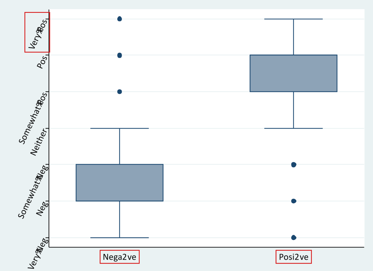
LLM-generated corrections to the published research of P. M. Aronow

Journal article P041

Corrections to: Editorial Bias in Crowd-Sourced Political Information

Joshua L. Kalla and P. M. Aronow (2015). Editorial Bias in Crowd-Sourced Political Information. PLOS ONE 10(9):e0136327.

DOI
10.1371/journal.pone.0136327
Audited edition
PLOS ONE, 2015, 10(9):e0136327; 8 pages in the audited file
SHA-256 of the audited file
9e916021e736e531a7833aac2bb408c78f91570d48fdbec9c4b2faf8726ab138
Permanent address
https://pmaronow.github.io/llm-audit/works/P041/

Summary

The paper reports four field experiments, and a partially aborted fifth, that added positive or negative facts described as true, cited or uncited, to the Wikipedia pages of U.S. senators and recorded the time to removal. It finds that negative facts are removed faster than positive ones on the pages of sitting senators (hazard ratio 1.59). 20 entries are classified as errors (1 Major, 2 Moderate, 17 Minor), and 2 are clarity notes. The most consequential is P041-E006: Study 3 (hazard ratio 0.69, 95% interval 0.28 to 1.70) does not show that the bias is limited to active politicians.

What was and was not checked

I checked the following points against the replication data and programs. This is not a statement that the rest of the paper is correct.

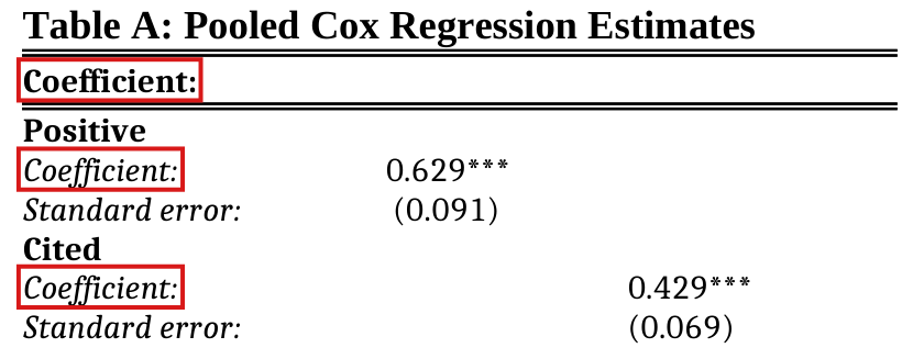
  • The pooled hazard ratios of Table A of S6 File, 0.6290.629 (0.091)(0.091) and 0.4290.429 (0.069)(0.069), reproduce, and the values 1.59 (p=0.001p=0.001) and 2.33 (p<0.001p<0.001) of the main text are their reciprocals after rounding. The pooled difference between positive and negative facts remains with standard errors clustered by senator. It also remains without the Study 1 edits of the last day and with Study 4 censored at the start of Study 5.
  • Table C of S6 File (Study 3) and the pp-values 0.420.42, 0.700.70 and 0.470.47 of the main text reproduce; for the conclusion drawn from them, see P041-E006.
  • The Cox estimates checked in S6–S10 Files reproduce to their printed precision from the commands as run. The exceptions and qualifications are in P041-E003, P041-E008, P041-E009 and P041-E012. One entry of Table B of S7 File (printed 0.3860.386) is 0.3890.389 in the re-estimate, a difference in the third decimal that I could not settle without Stata.
  • With Study 5 included, the pooled hazard ratio for positive facts is 0.5630.563, with separate study effects for its two halves. Adding only its first half to the citation analysis gives a hazard ratio of 0.4540.454 for cited facts. These estimates preserve the direction and significance of the pooled results.
  • The coefficients and robust standard errors of Tables A and B of S11 File reproduce, one standard error aside (P041-E011; for the description of the outcome, see P041-E010).
  • The treatment counts and assignment patterns in the data match those described. Study 1 has 25 blocks of four, with two positive and two cited facts in each. The valence assignments in Studies 2 and 5 reverse those in Studies 1 and 4, respectively. The first 50 edits of Study 5 have all four conditions and the last 50 only cited facts, and the edit dates are those stated in S1–S5 Files.
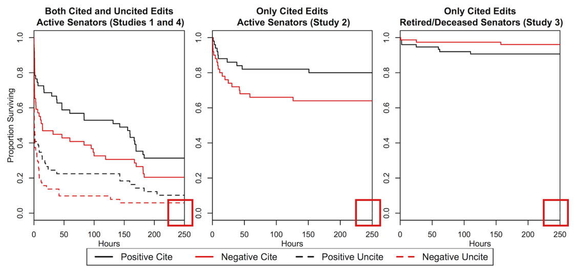
  • The Kaplan–Meier values recomputed from the data match the three panels of Fig 1 within the 250 hours shown.
  • In S12 File, the following reproduce: the 237 of 245 quality-control responses, the 551 facts rated five times each, the entries of Table A, the six Fleiss kappas, and the relevance means of the main text (5.0 and 5.0, with unclustered standard error 0.04). See P041-E013, P041-N015 and P041-E018.
  • The two example facts quoted on p. 3 are in the archived list of facts. The Harvard and Yale archives hold identical data, and only the main program differs between them.

The following limits apply.

  • The pre-analysis plan registered with EGAP and its addenda were not available. Statements that an analysis was “as specified in our registered pre-analysis plan” are unchecked.
  • The sources do not say when observation of the facts that were never removed ended, so I could not check the common censoring time that the Cox models give them.
  • The revision histories of the Wikipedia pages were not consulted. Who removed each fact, from which account each edit was made, and why, are not in the data.
  • The truth of each inserted fact was not checked against the news reports, and the summaries of the literature were not checked.
  • No Stata run was possible. The Stata programs were re-estimated in R and Python, and the embedded figures of S6 and S12 Files were seen only in approximate renderings.
  • Two XML codebooks named in the Harvard metadata are not in either archive.
  • I did not reproduce every cell or the likelihood-ratio tests of the balance tables in S1–S5 Files.
  • I read the Discussion’s suggestion that such biases may build over time as a possibility. I found no estimate of accumulation or downstream public perceptions in the paper.

Headline claims and related corrections

  1. On the pages of sitting U.S. senators, negative facts are removed faster than positive facts (pooled Studies 1, 2 and 4: hazard ratio 1.591.59, p=0.001p=0.001). The paper describes the pattern as consistent across studies and as evidence of an editorial bias toward positivity.

    S6 Table A column 1 (0.6290.629, standard error 0.0910.091); S6 Tables B, D, E; Fig 1; S11 Tables A, B

    See P041-E003, P041-E012, P041-N011.

  2. Negative facts are 36%36\% more likely than positive facts to be removed within 12 hours and 29%29\% more likely within 3 days.

    Abstract; replication do-file 'Main findings' block (lines 30-38); no table in the paper

    See P041-E001, P041-E002.

  3. Citations substantially lengthen survival: uncited facts are 64%64\% more likely than cited facts to be removed within four hours (reported hazard ratio 2.332.33, p<0.001p<0.001).

    S6 Table A column 2 (0.4290.429, standard error 0.0690.069); S6 Tables B, D, E; S11; Fig 1

    See P041-E001, P041-E003, P041-E010, P041-E011.

  4. The positivity bias remains among cited facts; the reported tests found no statistically detectable interaction between valence and citation.

    S7 Tables A, B; Study 2 column of S6 Table D

  5. The paper reports no editorial bias among retired and deceased senators in Study 3 and says that, if anything, positive facts were removed more quickly. It suggests that the bias is limited to active politicians and is not systemic to Wikipedia.

    S6 Table C; Fig 1 third panel; S11 Study 3 columns

    See P041-E005, P041-E006.

  6. Facing reelection in 2014 moderates the effect of citations (interaction hazard ratio 0.320.32, p<0.001p<0.001), suggesting that the citation policy is applied most when stakes are high. The paper reports no systematic evidence that other covariates moderate either effect.

    S8; S9 Tables A, B; S10

    See P041-E008, P041-E003, P041-E004, P041-E009, P041-N005.

  7. Independent Mechanical Turk raters saw the positive facts as more positive and more favorable to the senator than the negative facts, and as equally relevant (means 5.05.0 and 5.05.0 on a 7-point scale, standard error 0.040.04 each).

    Methods p. 3; S12 Table A, Figures A-C

    See P041-N015, P041-E018, P041-E013, P041-E014.

  8. Including the partially aborted Study 5 does not change the results.

    Methods p. 3; S5; Study 5 columns of S6 Tables D, E; S7; S9; S10

  9. The paper states that true, relevant and cited information about active senators was selectively removed from Wikipedia pages in the days and months leading up to the 2014 midterm elections.

    Discussion p. 5; fact-validation description p. 3; Fig 1; S6; S12 Figures A-C and Table A

    See P041-E018, P041-N015.

  10. Repeated editorial biases may accumulate and distort the political information available on crowd-sourced sites.

    Discussion pp. 5-6; Fig 1 and the repeated-study evidence in S6 Figure A and Tables D, E

Sources that could not be obtained

  • EGAP preregistration plan and addenda referenced by the article and S1-S5 (not an official supplement; all twelve official supplements are present)

Corrections

Major (1)

A central result, method or key claim fails for a non-trivial reason, and the repair changes what the paper establishes.

Study 3’s nondetection and smaller early absolute survival differences do not establish that editorial bias is limited to active politicians or is not systemic to Wikipedia, or exclude Wikipedia’s culture or its policy on biographies of living persons as explanations.

“Replication on Wikipedia Pages of Dead and Retired Senators”, last two sentences, p. 5 (PDF p. 5); Discussion, first paragraph, p. 5 (PDF p. 5)

See also under Formal statements (Lean): P041-T1, P041-T2, P041-T11

My comment on this entry

As printed

End of the section on Study 3, p. 5: “This suggests that the editorial bias cannot be explained by Wikipedia’s culture in general or by policies concerning biographies of living persons in particular. Instead, our findings suggest the editorial bias is limited to active politicians, the types of people for whom the stakes of a positive public image are the highest.”

Discussion, p. 5: “In a test conducted on the Wikipedia pages of recently retired and deceased senators, we find no editorial bias, suggesting that this bias is limited to the pages of active politicians and is not systemic to Wikipedia.”

The problem

Study 3 added facts to the pages of 151 former senators, and 20 of the facts were removed during the follow-up: 8 of 75 positive facts and 12 of 76 negative facts. The article reports that it finds no difference between the rates at which positive and negative facts are removed (p=0.70p=0.70 for living and p=0.47p=0.47 for deceased former senators, and p=0.42p=0.42 pooled). Read as a statement that the tests detected no difference, this is correct. The two passages above go further. They conclude that the bias found on the pages of sitting senators is absent elsewhere, and that Wikipedia’s culture and its policy on living persons are excluded as explanations. These conclusions need more than a test that detects no difference. They need evidence that the effect on the pages of former senators is absent, or smaller than the effect on the pages of sitting senators.

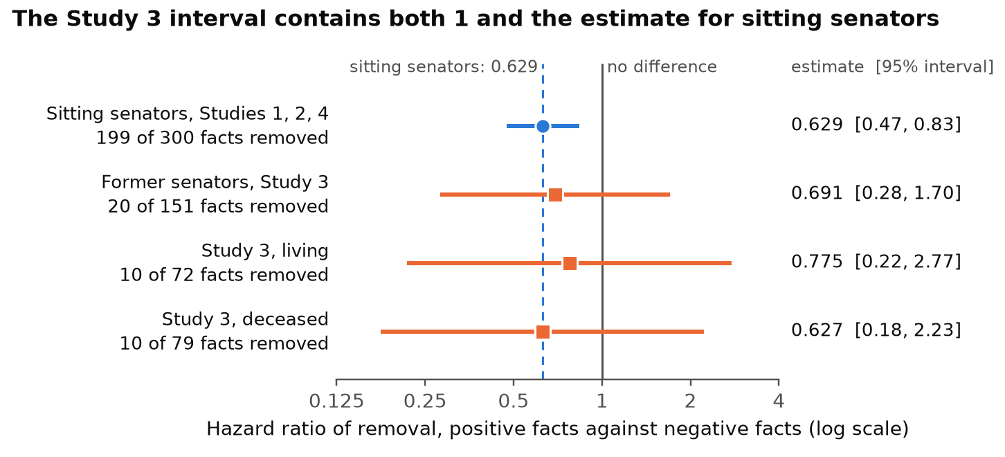
On the primary measure of the article, Study 3 gives no such evidence. The hazard ratio of removal for positive against negative facts is 0.691 for former senators (S6 Table C) and 0.629 for sitting senators (S6 Table A). The 95% interval for former senators runs from 0.28 to 1.70 and contains both 1 and 0.629. Comparing the two hazard ratios directly, I find a ratio of 1.12 with p=0.81p=0.81. Study 3 therefore cannot distinguish the absence of bias from a relative bias as large as the one found for sitting senators.

The data do contain evidence of a narrower kind. In the first days, the difference in survival between positive and negative facts was larger on the pages of sitting senators: 0.153 against −0.027-0.027 at 12 hours and 0.127 against −0.054-0.054 at 7 days, and a test rejects equality of these survival differences at both times. A smaller absolute difference does not show that relative bias is absent, because the same relative preference can produce a smaller absolute difference on pages that are edited less often. Further, the experiments randomized the valence of a fact and not the population of pages. The pages of sitting and of former senators differ in more than political activity. These comparisons therefore do not identify political activity as the cause of the bias, and they do not exclude Wikipedia’s culture or the enforcement of its policy on living persons as explanations. The second paragraph of the Discussion allows as much when it says that editors may apply the guidelines for living persons more conservatively to sitting senators.

Evidence an exact counterexample

The evidence is a recalculation from the replication files and an exact counterexample.

The recalculation reproduces the four printed hazard ratios and standard errors of S6 Tables A and C and the three pp-values of the main text. The figure shows the estimates with their 95% intervals. To compare the two populations, I fit a Cox model to Studies 1–4 with an interaction between valence and Study 3. The ratio between the hazard ratio for former senators and the hazard ratio for sitting senators is 1.12 (p=0.81p=0.81), or 1.09 (p=0.85p=0.85) when the baseline hazard is stratified by study. Treating the samples as independent and approximating the log hazard ratio standard errors by 0.318/0.6910.318/0.691 and 0.091/0.6290.091/0.629, the printed entries give

z=log⁡0.691−log⁡0.629(0.318/0.691)2+(0.091/0.629)2=0.09400.4824=0.19,p=0.85.z=\frac{\log 0.691-\log 0.629}{\sqrt{(0.318/0.691)^2+(0.091/0.629)^2}}=\frac{0.0940}{0.4824}=0.19,\qquad p=0.85 .

At 12 hours, the difference in survival between positive and negative facts is 23/150=0.15323/150=0.153 for sitting senators and −51/1900=−0.027-51/1900=-0.027 for former senators, and the gap between the two populations has p=0.0019p=0.0019. At 7 days the corresponding figures are 0.127, −0.054-0.054 and p=0.0038p=0.0038. When the comparison for sitting senators is restricted to cited facts, the differences are 0.140 and 0.138, with p=0.0097p=0.0097 and p=0.0091p=0.0091.

The counterexample shows that such a gap in absolute differences is compatible with one and the same relative bias. Suppose that, in each population, positive facts are removed at the constant hazard λ+=−2log⁡(q)/12\lambda_+=-2\log(q)/12 per hour and negative facts at the constant hazard λ−=−3log⁡(q)/12\lambda_-=-3\log(q)/12 per hour, where q=4/5q=4/5 for sitting senators and q=99/100q=99/100 for former senators. Then λ+/λ−=2/3\lambda_+/\lambda_-=2/3 in both populations. The probability that a fact survives 12 hours is S+(12)=exp⁡(−12λ+)=q2S_+(12)=\exp(-12\lambda_+)=q^2 for a positive fact and S−(12)=exp⁡(−12λ−)=q3S_-(12)=\exp(-12\lambda_-)=q^3 for a negative fact, which gives S+(12)−S−(12)=q2(1−q)S_+(12)-S_-(12)=q^2(1-q).

The counterexample: the same hazard ratio in both populations, and a much smaller absolute difference in survival at 12 hours where facts are removed less often.
PagesqqS+(12)S_+(12)S−(12)S_-(12)S+(12)−S−(12)S_+(12)-S_-(12)λ+/λ−\lambda_+/\lambda_-
Sitting senators4/54/516/2516/2564/12564/12516/125=0.12816/125=0.1282/32/3
Former senators99/10099/1009801/100009801/10000970299/1000000970299/10000009801/1000000=0.0098019801/1000000=0.0098012/32/3

The model illustrates the logical point and is not a fit to the data.

What survives

The bias on the pages of sitting senators stands (hazard ratio 0.629, p=0.001p=0.001). The statement that Study 3 detected no difference also stands, and so does the sentence of the abstract that reports “no evidence of an editorial bias” for former senators, read as a statement that none was detected. The early absolute differences in survival were smaller on the pages of former senators, also when the comparison is restricted to cited facts. The findings on citations do not depend on this interpretation. What is given up is the conclusion that the bias is limited to active politicians and is not systemic to Wikipedia, and the exclusion of Wikipedia’s culture and of its policy on living persons as explanations. No data and no estimate change.

Corrected

End of the section on Study 3, in place of the two sentences: “Study 3 detected no statistically clear difference between positive and negative facts over the full follow-up. Its estimate of the relative effect is imprecise and does not exclude the estimate for sitting senators. Early absolute differences in survival were smaller on the sampled pages of former senators, also when the comparison is restricted to cited facts. These comparisons do not establish that relative bias is absent on the pages of former senators, do not identify political activity as the cause of the bias, and do not exclude Wikipedia’s culture or the enforcement of its policy on biographies of living persons as explanations.”

Discussion, p. 5: “In a test conducted on the Wikipedia pages of recently retired and deceased senators, no editorial bias was detected; the estimate is too imprecise to show that this bias is limited to the pages of active politicians or that it is not systemic to Wikipedia.”
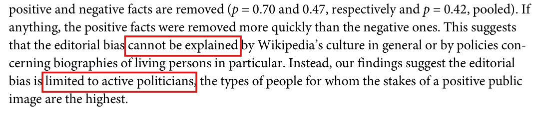

Six lines of the article. Red boxes mark the words 'cannot be explained' in the sentence 'This suggests that the editorial bias cannot be explained by Wikipedia's culture in general or by policies concerning biographies of living persons in particular', and the words 'limited to active politicians' in the sentence that follows.
End of the section “Replication on Wikipedia Pages of Dead and Retired Senators”, p. 5 (PDF p. 5). The marked words carry the two conclusions that Study 3 does not support.
Five lines of the article. A red box marks the clause 'is limited to the pages of active politicians and is not systemic to Wikipedia', which ends the sentence that begins 'In a test conducted on the Wikipedia pages of recently retired and deceased senators'.
Discussion, first paragraph, p. 5 (PDF p. 5). The marked clause repeats the conclusion.
A chart with four horizontal intervals on a logarithmic axis from 0.125 to 4. Sitting senators, Studies 1, 2, 4, 199 of 300 facts removed: 0.629, interval 0.47 to 0.83, a short blue interval that lies entirely below 1. Former senators, Study 3, 20 of 151 facts removed: 0.691, interval 0.28 to 1.70. Study 3, living, 10 of 72 removed: 0.775, interval 0.22 to 2.77. Study 3, deceased, 10 of 79 removed: 0.627, interval 0.18 to 2.23. The three orange intervals for Study 3 are wide and cross both the solid vertical line at 1 and the dashed vertical line at 0.629, the estimate for sitting senators.
Hazard ratios of removal for positive against negative facts, with 95% intervals, from a recalculation on the replication files. The four estimates are the entries printed in S6 Tables A and C. The dashed line is the estimate for sitting senators, and the solid line is a ratio of 1.
My comment and the history of this entry

Agreed.

  1. Classification before my review (the classification when the audit was first completed, before I reviewed it): Major error.
  2. I commented.
  3. Independent evaluation. No change was needed: my comment agrees with the entry.

Moderate (2)

A real substantive error with limited reach.

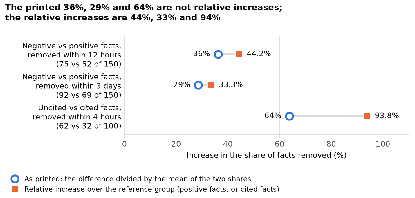
The printed 36%, 29% and 64% are differences divided by the mean of the two shares of facts removed; relative to the positive facts and to the cited facts, the increases in the share removed are 44%, 33% and 94%.

Abstract, p. 1 (PDF p. 1); Results, “Effects of Citations on Survival”, pp. 4–5 (PDF pp. 4–5); replication program Kalla_Aronow_PLOS_2015.do, lines 33, 38 and 43

See also under Formal statements (Lean): P041-T3, P041-T4, P041-T12

As printed

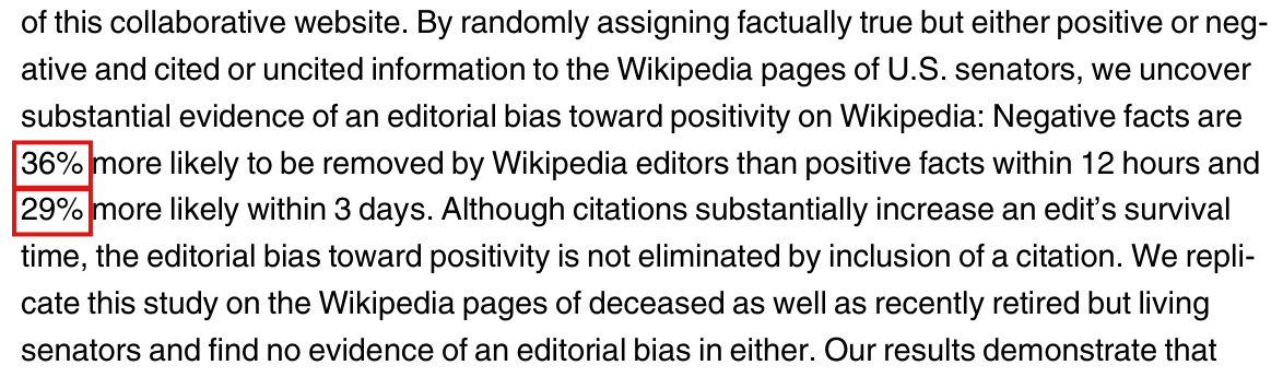
Abstract, p. 1: Negative facts are 36% more likely to be removed by Wikipedia editors than positive facts within 12 hours and 29% more likely within 3 days.

Results, pp. 4–5: Consistent with Wikipedia’s policy, uncited (but true) facts are 64% more likely to be removed than cited facts within four hours (hazard ratio = 2.33, p<0.001p<0.001).

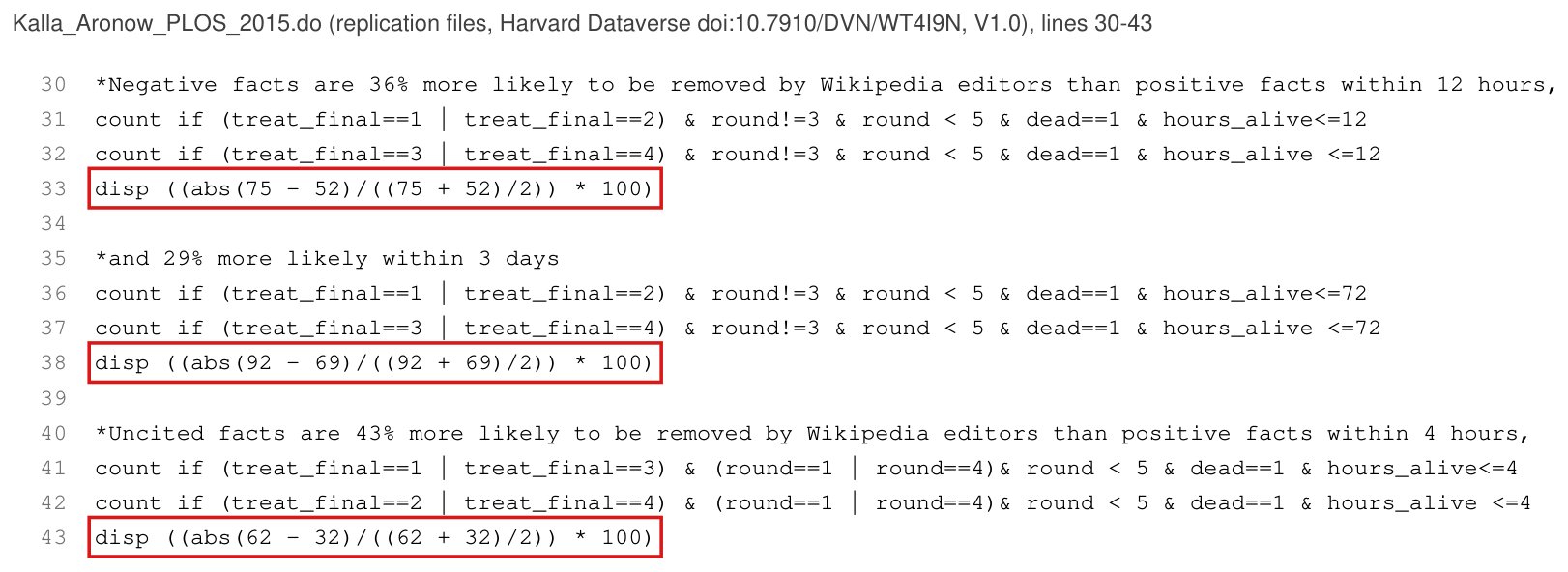
Replication program, lines 33, 38 and 43:

disp ((abs(75 - 52)/((75 + 52)/2)) * 100)

disp ((abs(92 - 69)/((92 + 69)/2)) * 100)

disp ((abs(62 - 32)/((62 + 32)/2)) * 100)

The problem

The sentence “AA is xx% more likely to be removed than BB within a given time” compares the shares of facts removed by that time, with BB as the reference group. If pAp_A and pBp_B are the two shares, it means that pA=(1+x/100) pBp_A=(1+x/100)\,p_B, that is, x=100 (pA/pB−1)x=100\,(p_A/p_B-1). The three printed figures were computed differently. Let aa and bb be the numbers of facts removed in the two groups. The replication program evaluates 100 ∣a−b∣/{(a+b)/2}100\,|a-b|/\{(a+b)/2\}, the difference divided by the mean of the two counts. Since the groups have equal sizes, this equals 100 ∣pA−pB∣/{(pA+pB)/2}100\,|p_A-p_B|/\{(p_A+p_B)/2\}, a symmetric percentage difference. When pA>pB>0p_A>p_B>0, the symmetric difference is smaller than the relative increase. The counts are 75 negative against 52 positive facts of 150 at 12 hours, 92 against 69 of 150 at 72 hours, and 62 uncited against 32 cited facts of 100 at four hours. The printed 36%, 29% and 64% are the symmetric differences 36.22%, 28.57% and 63.83%, rounded. The relative increases are 44.23%, 33.33% and 93.75%, and rounding does not account for the gap. The article gives no convention under which “xx% more likely” means a symmetric difference. Someone who quotes the three figures as relative increases quotes numbers that are too small.

Evidence a recalculation from the source

The evidence is a recount from the replication data and exact arithmetic. I count a fact as removed by a horizon when its removal is recorded and its stored survival time is at most the horizon, as the program does. For negative against positive facts, Studies 1, 2 and 4 are pooled, with 150 facts in each group. For uncited against cited facts, Studies 1 and 4 are pooled, with 100 facts in each group. The counts agree with the numbers written into the program. Since the groups have equal sizes, I have pA/pB=a/bp_A/p_B=a/b, and a direct computation gives

100(7552−1)=57513=44.23…,100(9269−1)=1003=33.33…,100(6232−1)=3754=93.75.\begin{aligned} 100\Bigl(\frac{75}{52}-1\Bigr)&=\frac{575}{13}=44.23\ldots,\\ 100\Bigl(\frac{92}{69}-1\Bigr)&=\frac{100}{3}=33.33\ldots,\\ 100\Bigl(\frac{62}{32}-1\Bigr)&=\frac{375}{4}=93.75 . \end{aligned}

Evaluating the three expressions in the program, I find

100⋅23127/2=4600127=36.22…,100⋅23161/2=2007=28.57…,100⋅3094/2=300047=63.83….\begin{aligned} \frac{100\cdot 23}{127/2}&=\frac{4600}{127}=36.22\ldots,\\ \frac{100\cdot 23}{161/2}&=\frac{200}{7}=28.57\ldots,\\ \frac{100\cdot 30}{94/2}&=\frac{3000}{47}=63.83\ldots . \end{aligned}

Each printed integer is a rounded value from the second display, and none is a rounded value from the first. To compare the two measures in general, let pA>pB>0p_A>p_B>0 and d=pA−pBd=p_A-p_B, and write R=100 d/pBR=100\,d/p_B and M=200 d/(pA+pB)M=200\,d/(p_A+p_B). Then

R−M=100 d2pB (pA+pB)>0.R-M=\frac{100\,d^{2}}{p_B\,(p_A+p_B)}>0 .

This implies that the symmetric difference is the smaller of the two measures. The Harvard and the Yale copies of the replication program contain the same three expressions.

Facts removed in the comparison group and in the reference group (positive facts in the first two rows, cited facts in the third), the printed figure, the difference divided by the mean of the two shares, and the relative increase.
ComparisonRemovedReferencePrintedOver the meanRelative
Negative vs positive, 12 hours75 of 15052 of 15036%36.22%44.23%
Negative vs positive, 3 days92 of 15069 of 15029%28.57%33.33%
Uncited vs cited, 4 hours62 of 10032 of 10064%63.83%93.75%
What survives

Correcting only these percentages leaves the three pairs of counts, the direction of the three comparisons, the Kaplan–Meier curves, and the Cox estimates with their pp-values (hazard ratios 1.59 and 2.33) unchanged; I have not checked the correctness of those other results here. The corrected increases are larger than the printed ones. If the survival times are rebuilt from the recorded minutes (P041-E002), converted from milliseconds to hours by division by 3,600,0003{,}600{,}000, and counted with an inclusive 12-hour cutoff, then 76 negative facts are removed within 12 hours and the first increase is 600/13=46.15…600/13=46.15\ldots%.

Corrected

Abstract, p. 1: Negative facts are 44% more likely to be removed by Wikipedia editors than positive facts within 12 hours and 33% more likely within 3 days.

Results, pp. 4–5: Consistent with Wikipedia’s policy, uncited (but true) facts are 94% more likely to be removed than cited facts within four hours (hazard ratio = 2.33, p<0.001p<0.001).

Here the increase is computed relative to the reference group. Let p1p_1 be the share of facts removed by the stated time in the comparison group (negative facts, or uncited facts) and p0>0p_0>0 the share in the reference group (positive facts, or cited facts). The increase is

100(p1p0−1)=100 p1−p0p0,100\Bigl(\frac{p_1}{p_0}-1\Bigr)=100\,\frac{p_1-p_0}{\colorbox{#ffe58a}{$\displaystyle p_0$}} ,

which gives 44.23%, 33.33% and 93.75% with the stored survival times. In lines 33, 38 and 43 of the replication program, the divisor is the count for the reference group: 100 (75−52)/52100\,(75-52)/\colorbox{#ffe58a}{$52$}, 100 (92−69)/69100\,(92-69)/\colorbox{#ffe58a}{$69$} and 100 (62−32)/32100\,(62-32)/\colorbox{#ffe58a}{$32$}. An alternative is to keep 36%, 29% and 64% and to describe them as differences relative to the mean of the two shares, which reports a different measure.

Crop of eight lines of the abstract. Red boxes mark '36\%' at the start of the line 'more likely to be removed by Wikipedia editors than positive facts within 12 hours and' and '29\%' at the start of the next line, 'more likely within 3 days'.
Abstract, p. 1 (PDF p. 1). The marked figures are the 36% and 29% said to be the increases in the likelihood of removal within 12 hours and within 3 days.
Crop of the last three lines of page 4. A red box marks '64\%' in 'uncited (but true) facts are 64\% more likely to be', where the page ends.
Results, “Effects of Citations on Survival”, last lines of p. 4 (PDF p. 4). The marked figure is the 64%; the sentence continues on p. 5 with “removed than cited facts within four hours (hazard ratio = 2.33, p<0.001p<0.001)”.
Listing of lines 30 to 43 of the Stata program. Red boxes mark line 33, 'disp ((abs(75 - 52)/((75 + 52)/2)) * 100)', line 38, 'disp ((abs(92 - 69)/((92 + 69)/2)) * 100)', and line 43, 'disp ((abs(62 - 32)/((62 + 32)/2)) * 100)'. The comment lines above them read 'Negative facts are 36\% more likely to be removed', 'and 29\% more likely within 3 days' and 'Uncited facts are 43\% more likely to be removed'.
Replication program Kalla_Aronow_PLOS_2015.do, lines 30–43, typeset from the file. The marked lines compute the three percentages: each divides the difference of the two counts by their mean.
Dot plot with three rows and a horizontal axis labeled from 0 to 100 per cent. Negative against positive facts within 12 hours (75 against 52 of 150 removed): circle labeled 36 per cent, relative increase 44.2 per cent. Negative against positive facts within 3 days (92 against 69 of 150): circle labeled 29 per cent, relative increase 33.3 per cent. Uncited against cited facts within 4 hours (62 against 32 of 100): circle labeled 64 per cent, relative increase 93.8 per cent. In each row the square for the relative increase lies to the right of the open circle for the symmetric difference.
The three comparisons, from the recount of the replication data. Open circles: the difference of the two shares removed divided by their mean, labeled with the rounded printed figures. Squares: the increase relative to the share removed in the reference group.

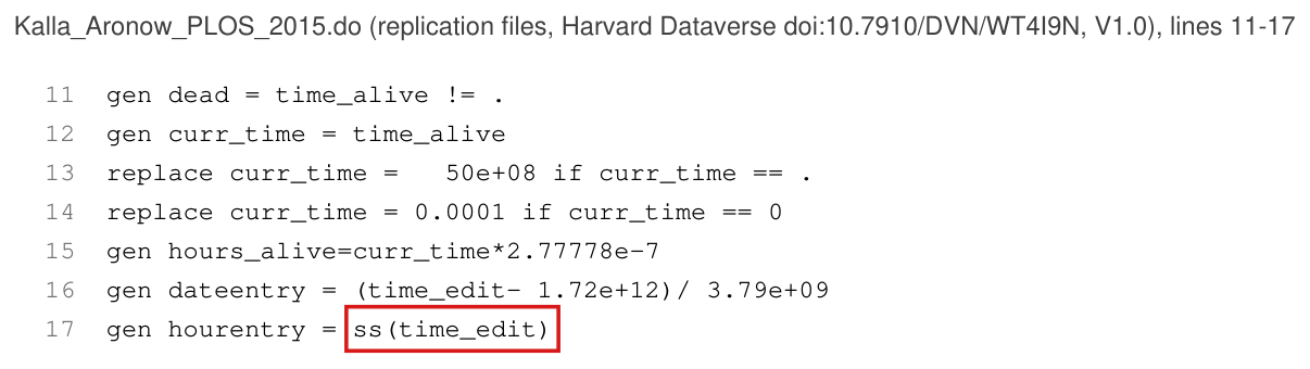
The control described as the hour (time) of entry in the covariate-adjusted models is the seconds within the minute of the stored edit time; with the hour of entry the adjusted estimates change, and the 10% marker in column 2 of S7 Table B is lost.

Replication program Kalla_Aronow_PLOS_2015.do, line 17; S6 File, Tables B and E and their notes; S7 File, Table B; S8 File, columns 3 and 4; Results, “Survival of Positive and Negative Facts on Wikipedia”, p. 4 (PDF p. 4)

As printed

Replication program, line 17:

gen hourentry = ss(time_edit)

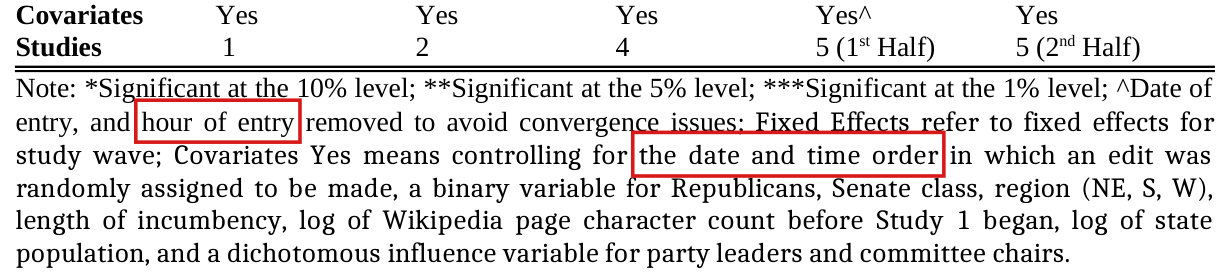
S6 File, note to Table E: ∧{}^{\wedge}Date of entry, and hour of entry removed to avoid convergence issues

S6, S7 and S8 Files, notes to the tables: Covariates Yes means controlling for the date and time order in which an edit was randomly assigned to be made, a binary variable for Republicans, Senate class, region (NE, S, W), length of incumbency, log of Wikipedia page character count before Study 1 began, log of state population, and a dichotomous influence variable for party leaders and committee chairs.

Results, p. 4 (context): We find no systematic evidence that this effect is moderated by covariates (state population, Senate class, character count of page, geographic region, length of incumbency, political party, date of entry, and time of entry; see Table A in S9 File and S10 File), as specified in our registered pre-analysis plan.

The problem

In Stata, ss() returns the seconds component of a datetime and hh() returns the hour. Line 17 of the replication program therefore sets the variable hourentry to the seconds within the minute of the stored edit time. The supplements call this control the “hour of entry” (note to Table E of S6 File) and the “date and time order” of the edit. The main text speaks of the time of day (p. 3) and of the “time of entry” (p. 4). The recorded edit-time strings have zero seconds. The fitted seconds values are the remainders left by the single-precision rounding of the stored times (P041-E002). They range from 0.0320.032 to 59.90459.904, and their correlation with the fractional hour of day is −0.03-0.03. Every adjusted model that includes hourentry controls for a different variable from the one described. These are the two models of Table B of S6 File, the models of Table E for Studies 1, 2, 4 and the second half of Study 5, the two models of Table B of S7 File, and columns 3 and 4 of S8 File. The printed entries of these models are those of a specification that the paper does not describe. The Table E model for the first half of Study 5 omits the date and the hour, as its note says, and is not affected. The analyses of S9 and S10 Files do not use the variable; on whether a test of the “time of entry” as a moderator is reported, see P041-N005.

Evidence an exact counterexample

The evidence is an exact example from the data and a re-estimation of the affected models. For a datetime tt in milliseconds, the two functions are

ss⁡(t)=t mod 60,0001000,hh⁡(t)=⌊t3,600,000⌋ mod 24.\operatorname{ss}(t)=\frac{t \bmod 60{,}000}{1000},\qquad \operatorname{hh}(t)=\Bigl\lfloor \frac{t}{3{,}600{,}000}\Bigr\rfloor \bmod 24 .

The Study 5 edit on the page of Al Franken was recorded at 17:18 on 7 November 2014. Its stored time is t=1,730,999,877,632t=1{,}730{,}999{,}877{,}632, that is, 17:17:57.632, and

t=28,849,997×60,000+57,632,ss⁡(t)=57.632,hh⁡(t)=17.t=28{,}849{,}997\times 60{,}000+57{,}632,\qquad \operatorname{ss}(t)=57.632,\qquad \operatorname{hh}(t)=17 .

The program assigns 57.63257.632 to an edit made in hour 17. In all 551 rows the value of ss(time_edit) differs from the hour.

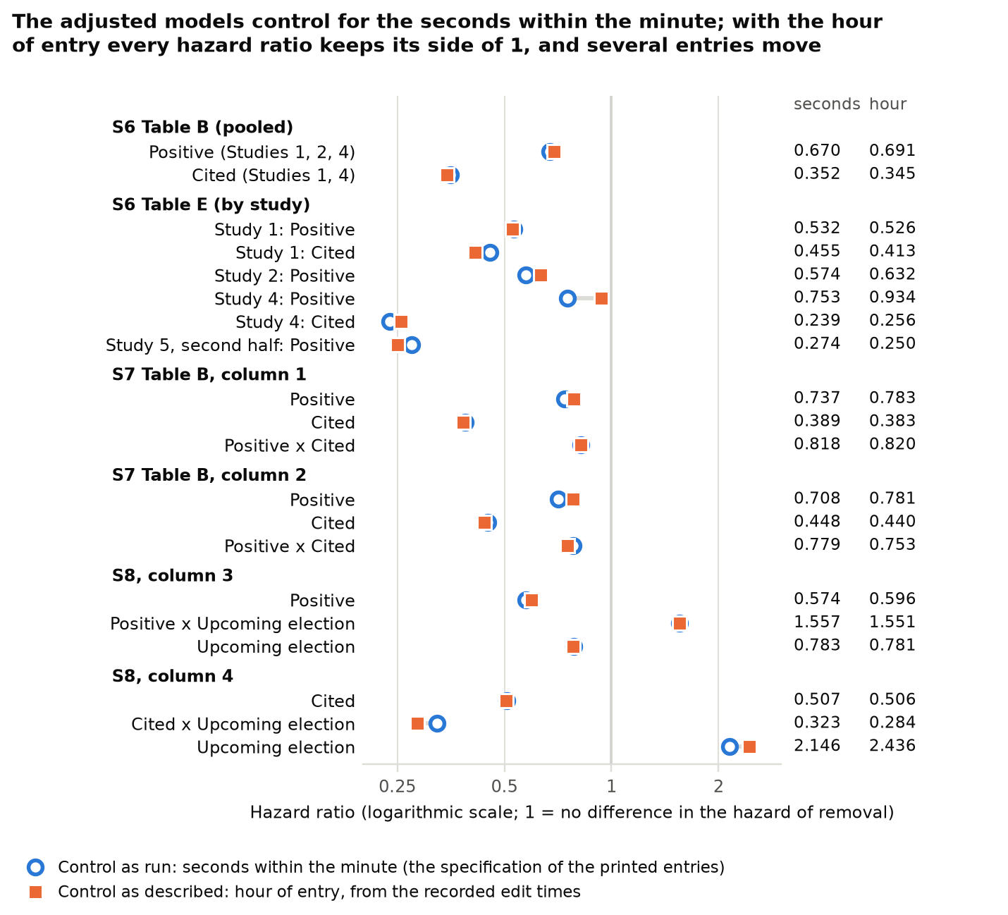
I re-estimated the Cox models in R with Breslow ties and robust standard errors scaled as in Stata. With the seconds as the control, I obtain the printed entries of Table B of S6 File, 0.6700.670 (0.095)(0.095) and 0.3520.352 (0.055)(0.055). The other hazard ratios shown also agree at three decimals, one entry of S7 Table B aside (printed 0.3860.386, re-estimated 0.3890.389). I then replaced the control by the integer hour of day, rebuilt from the strings that record the edit times. The table lists selected changes, and the figure shows all 20. Every hazard ratio keeps its side of 1, and every conclusion at the 5% level that I checked is unchanged. The pp-value of “Positive” in column 2 of S7 Table B rises from 0.0950.095 to 0.2140.214. Applying hh() to the stored times is not enough, since rounding moves three edits across an hour boundary. With a fractional hour (hour plus minutes over 60), the two pooled entries are 0.6910.691 and 0.3440.344, nearly the same as with the integer hour.

Hazard ratios (standard errors) of adjusted models with the control as run and with the hour of entry, and the two pp-values.
EntrySeconds, as printedHour of entrypp, secondspp, hour
S6 Table B, Positive0.670 (0.095)0.691 (0.097)0.00450.0085
S6 Table B, Cited0.352 (0.055)0.345 (0.052)<0.001<0.001<0.001<0.001
S6 Table E, Study 4, Positive0.753 (0.200)0.934 (0.267)0.290.81
S7 Table B, column 2, Positive0.708 (0.146)0.781 (0.156)0.0950.214
S8, column 4, Cited ×\times Upcoming Election0.323 (0.104)0.284 (0.088)<0.001<0.001<0.001<0.001
What survives

The unadjusted estimates of Table A of S6 File, and with them the hazard ratios 1.59 and 2.33 of the main text, do not use the variable. The same holds for the Kaplan–Meier curves, the balance tables, Study 3, the unadjusted interactions, the regressions of S11 File and the tables of S9 and S10 Files. In the affected models the pooled effects of positive and cited facts stay significant, and no sign changes. All 20 hazard ratios of those models change at three decimals. For example, the Study 4 hazard ratio for positive facts in Table E moves from 0.750.75 to 0.930.93. The interaction of citation with an upcoming election, which the main text quotes as 0.320.32 (p. 5), becomes 0.280.28, and “Positive” in column 2 of S7 Table B is no longer significant at the 10% level.

Corrected

Replication program, line 17, with the hour of day taken from a double-precision datetime parsed from the recorded edit-time string time:

gen double time_edit_exact = clock(time, "hmDMY")

gen byte hourentry = hh(time_edit_exact)

The two lines state the intended computation; the re-estimates use the same construction outside Stata. With this control, the models that include hourentry are estimated again, and their estimates, standard errors and significance markers replace the printed ones. The pooled entries of Table B of S6 File become 0.6910.691 (0.097)(0.097) for positive facts and 0.3450.345 (0.052)(0.052) for cited facts; in column 2 of S7 Table B, “Positive” becomes 0.7810.781 (0.156)(0.156), without a marker; in column 4 of S8 File the interaction of citation with an upcoming election becomes 0.2840.284 (0.088)(0.088), and the main text (p. 5) reads “interaction term hazard ratio = 0.28, p<0.001p<0.001”. The remaining hazard ratios are in the figure. The note to Table E for the first half of Study 5 stands.

Listing of lines 11 to 17 of the Stata program. A red box marks 'ss(time\_edit)' in line 17, 'gen hourentry = ss(time\_edit)'.
Replication program Kalla_Aronow_PLOS_2015.do, lines 11–17, typeset from the file. The marked term defines the variable hourentry with the function that returns seconds.
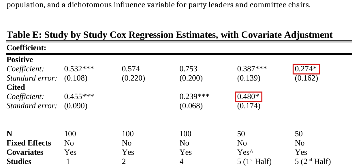
Crop of the rows 'Covariates' and 'Studies' of Table E and the six-line note below them. Red boxes mark 'hour of entry' in 'Date of entry, and hour of entry removed to avoid convergence issues' and 'the date and time order' in 'Covariates Yes means controlling for the date and time order in which an edit was randomly assigned to be made'.
S6 File, last rows of Table E and its note, from a rendering of the published Word file (the supplement has no fixed page numbers). The marked words name the control as the hour of entry and as part of the date and time order of the edit.
Crop of four lines of page 4. A red box marks 'date of entry, and time of entry' in the list of covariates 'state population, Senate class, character count of page, geographic region, length of incumbency, political party, date of entry, and time of entry'.
Results, p. 4 (PDF p. 4). The marked words list entry date and time among possible moderators, providing context for the intended meaning of time of entry.
Dot plot of 20 hazard ratios on a logarithmic axis from 0.2 to 3, in six groups: S6 Table B (pooled), S6 Table E (by study), S7 Table B columns 1 and 2, and S8 columns 3 and 4. Each row has an open circle for the model with the seconds control and a square for the model with the hour of entry, and the two values are printed at the right. No pair lies on opposite sides of 1. Examples include Study 4 Positive in S6 Table E, 0.753 to 0.934; Positive in S7 Table B column 2, 0.708 to 0.781; Cited by Upcoming election in S8 column 4, 0.323 to 0.284; and Upcoming election in S8 column 4, 2.146 to 2.436. The pooled entries of S6 Table B move from 0.670 to 0.691 and from 0.352 to 0.345.
The 20 hazard ratios of the adjusted models that include the control, re-estimated with the seconds within the minute (open circles) and with the hour of entry (squares); the two columns of numbers give the values. S7 Table B, column 1, pools Studies 1 and 4, and column 2 adds the first half of Study 5; S8, column 3, pools Studies 1, 2 and 4, and column 4 Studies 1 and 4. The values with the seconds equal the printed entries at three decimals in 19 rows; the exception is “Cited” in column 1 of S7 Table B, printed 0.386.

Minor (17)

Real but inconsequential, for example a misprint that does not change a result.

The replication data store the edit and removal times in single precision, so that the stored survival times differ from the recorded ones by up to 129 seconds; one 12-hour count changes from 75 to 76, and the pooled hazard ratios change in the third decimal.

“Estimation of Experimental Effects”, p. 4 (PDF p. 4); replication files: the three time variables of the data file, the codebook (p. 1), and lines 12 and 15 of the main Stata program

See also under Formal statements (Lean): P041-T4

As printed

Article, p. 4: Our primary dependent variable is the survival time of the facts–the amount of time between when the fact is added to Wikipedia and when it is removed.

Codebook, p. 1:

time_edit: Date and time the edit was made, in Stata format

time_removed: Date and time the edit was removed, in Stata format. Coded as missing if the edit was not removed.

time_alive: Difference between time_removed and time_edit. Amount of time the edit was alive on the Wikipedia page.

Replication program, lines 12 and 15:

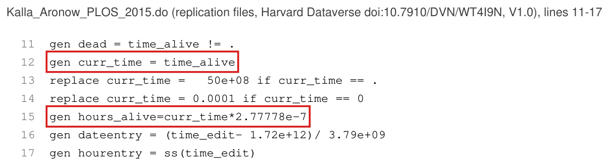
gen curr_time = time_alive

gen hours_alive=curr_time*2.77778e-7

The problem

The article’s definition of the survival time is correct; the stored values are not exact. The data file holds the three variables as Stata floats, which have 24 significant binary digits. A Stata datetime counts milliseconds from 1 January 1960, and the 2014 values lie between 2402^{40} and 2412^{41}, where consecutive floats are 217=131,0722^{17}=131{,}072 milliseconds apart. The edit and removal times were recorded to the minute (the string variables time and removed). Each stored time is the recorded minute rounded to the nearest multiple of 131,072131{,}072 ms, and time_alive is the difference of the two rounded times. Of the 294 survival times, 286 differ from the difference of the recorded minutes, by between −126,752-126{,}752 and +128,960+128{,}960 ms, and 15 stored survival times are zero where the recorded minutes give 8. The multiplier 2.77778×10−72.77778\times10^{-7} in line 15 is a rounded value of 1/3,600,0001/3{,}600{,}000 and moves a survival time of exactly 12 hours above 12.

Evidence an exact counterexample

The evidence is an exact counterexample from the data, with a recalculation. Set q=217=131,072q=2^{17}=131{,}072. For the fact on the page of Jon Tester in Study 5, the recorded times are 18:49 and 20:47 on 6 November 2014, which are 118 minutes apart. In milliseconds the two times are

X1=1,730,918,940,000=13,205,863 q+64,864,X2=1,730,926,020,000=13,205,917 q+66,976.\begin{aligned} X_1&=1{,}730{,}918{,}940{,}000=13{,}205{,}863\,q+64{,}864,\\ X_2&=1{,}730{,}926{,}020{,}000=13{,}205{,}917\,q+66{,}976 . \end{aligned}

Since 64,864<q/2<66,97664{,}864<q/2<66{,}976, the first is rounded down and the second up. The stored times are 13,205,863 q13{,}205{,}863\,q and 13,205,918 q13{,}205{,}918\,q, and I obtain

time_alive=55 q=7,208,960 ms,X2−X1=7,080,000 ms,\texttt{time\_alive}=55\,q=7{,}208{,}960\ \text{ms},\qquad X_2-X_1=7{,}080{,}000\ \text{ms},

an error of 128,960128{,}960 ms, or 128.96128.96 seconds. For the negative, cited fact on the page of Dan Coats in Study 1, the recorded times are 21:23 on 9 July and 09:23 on 10 July 2014, exactly 12 hours apart, and

X1=1,720,560,180,000=13,126,832 q+56,096,X2=1,720,603,380,000=13,127,162 q+2,336.\begin{aligned} X_1&=1{,}720{,}560{,}180{,}000=13{,}126{,}832\,q+56{,}096,\\ X_2&=1{,}720{,}603{,}380{,}000=13{,}127{,}162\,q+2{,}336 . \end{aligned}

Both are rounded down, so that time_alive=330 q=43,253,760\texttt{time\_alive}=330\,q=43{,}253{,}760 ms, which exceeds 43,200,00043{,}200{,}000 ms. The program counts a removal within 12 hours when hours_alive is at most 12, and this fact is not counted. With the recorded minutes it is counted. The number of negative facts removed within 12 hours in Studies 1, 2 and 4 is then 76, against 75 from the stored values, and the number of positive facts stays at 52. Among the horizons of 4, 6, 12, 24, 72 and 168 hours, the only other change is one Study 5 fact at 4 hours, outside the pooled samples. The multiplier alone would also misplace the Coats fact, since 43,200,000×2.77778×10−7=12.000009643{,}200{,}000\times2.77778\times10^{-7}=12.0000096.

I re-estimated the two pooled Cox models of Table A of S6 File with survival times rebuilt from the recorded minutes and nothing else changed (Breslow ties, robust standard errors). The hazard ratio for positive facts moves from 0.6289420.628942 to 0.6278650.627865 (p=0.0013p=0.0013) and that for cited facts from 0.4292270.429227 to 0.4275300.427530 (p<0.001p<0.001). Their reciprocals are 1.5931.593 and 2.3392.339, against the printed 1.59 and 2.33. In the 12-hour regressions of the kind reported in S11 File, the coefficient for positive facts moves from 0.1530.153 to 0.1600.160 and that for cited facts from 0.370.37 to 0.360.36, and both pp-values stay below 0.010.01.

What survives

The designs, the treatment assignments and the removal indicators are unchanged. The hazard of removal remains lower for positive facts and for cited facts, and both pooled effects remain statistically significant. The 3-day counts (69 and 92) and the 4-hour citation counts (32 and 62) are unchanged, and no fact changes its classification at 6, 24 or 168 hours. Every analysis of the survival times inherits the rounding, and its entries can change in the last digits; I recomputed only the quantities listed above. The seconds within each minute were never recorded, and the correction does not restore them.

Corrected

Rebuild time_edit and time_removed from the recorded strings time and removed as millisecond datetimes in double precision, keeping a missing value where the fact was not removed. Set time_alive to the difference of the rebuilt times, and compute the hours as this difference divided by 3,600,0003{,}600{,}000, in double precision. Converting the stored floats to doubles does not recover the recorded minutes. For the reported Cox recalculation, retain the program’s censoring time of 5×1095\times10^9 ms and replace zero durations by 0.00010.0001 ms before converting to hours. Equal rebuilt durations are ties at the recorded resolution of one minute. With these survival times, 76 of the 150 negative facts of Studies 1, 2 and 4 are removed within 12 hours (stored values: 75), and the pooled hazard ratios of Table A of S6 File are 0.6280.628 and 0.4280.428 (stored values: 0.6290.629 and 0.4290.429).

Crop of the heading 'Estimation of Experimental Effects' and the three lines below it. A red box marks 'survival time of the facts' in 'Our primary dependent variable is the survival time of the facts, the amount of time between when the fact is added to Wikipedia and when it is removed'.
“Estimation of Experimental Effects”, p. 4 (PDF p. 4). The marked words name the quantity whose stored values are affected; the definition itself is correct.
Crop of six lines of the codebook. Red boxes mark the variable names 'time\_edit:', 'time\_removed:' and 'time\_alive:' at the start of their definitions, 'Date and time the edit was made, in Stata format', 'Date and time the edit was removed, in Stata format' and 'Difference between time\_removed and time\_edit'.
Codebook of the replication files (Kalla_Aronow_PLOS_2015.pdf), p. 1. The marked names are the three variables that the data file stores in single precision.
Listing of lines 11 to 17 of the Stata program. Red boxes mark line 12, 'gen curr\_time = time\_alive', and line 15, 'gen hours\_alive=curr\_time*2.77778e-7'.
Replication program Kalla_Aronow_PLOS_2015.do, lines 11–17, typeset from the file. The marked lines take the stored survival time and convert it to hours with a rounded multiplier.

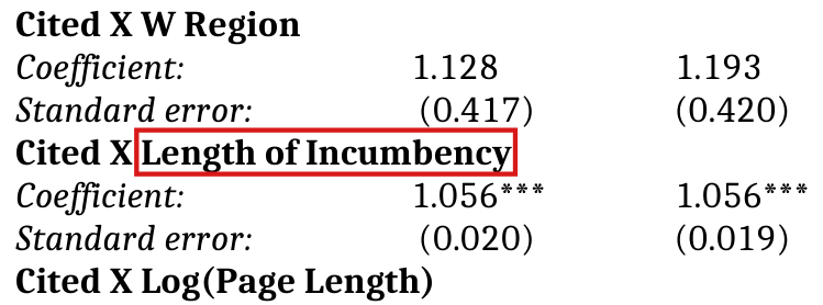
The covariate labelled length of incumbency in the Cox models of S9 and S10 Files is the year in which the senator was first elected, and a larger value means a shorter tenure: label the rows “First-election year”.

S9 File, Tables A and B, rows “Positive X Length of Incumbency” and “Cited X Length of Incumbency”; S10 File, row “Incumbency Length”; cited from p. 4 (PDF p. 4), “length of incumbency”

See also under Formal statements (Lean): P041-T10

As printed
  • S9 File, Table A: “Positive X Length of Incumbency”. Coefficient: 0.989, 0.981. Standard error: (0.019), (0.017).
  • S9 File, Table B: “Cited X Length of Incumbency”. Coefficient: 1.056***, 1.056***. Standard error: (0.020), (0.019).
  • S10 File: “Incumbency Length”. Coefficient: 1.004. Standard error: (0.008).
  • Codebook: “lengthofincumbency: Year Senator was first elected.”
  • Do-file, line 8: gen yearsinsenate=2014-lengthofincumbency
The problem

The codebook defines lengthofincumbency as the year in which the senator was first elected, and its values in the data are calendar years, 1993 and 2013 for example. The do-file builds a tenure, yearsinsenate, as 2014 minus that year, but uses it only in the balance checks. The Cox commands behind S9 and S10 Files use the year. A row labelled length of incumbency is read per additional year of tenure. In S9 File the entry is read as the factor by which the hazard ratio of the treatment changes, and in S10 File as the hazard ratio itself. Each of the five printed entries is the corresponding factor per later year of first election, and the factor per year of tenure is its reciprocal. The direction is therefore read backwards in all three rows, among them the one starred row, 1.056***. The entries are hazard ratios, as in the other Cox tables.

Evidence a recalculation from the source

The evidence is a recalculation from the replication data and a derivation. Refitting the five models with the year of first election reproduces all five printed pairs of estimate and standard error to three decimals. Let YY be the year of first election, L=2014−YL=2014-Y the tenure, TT the treatment indicator (positive or cited) and zz the remaining terms of the linear predictor. I write the fitted hazard as h(t∣T,Y,z)=h0(t)exp⁡(bY+aT+gTY+z)h(t\mid T,Y,z)=h_0(t)\exp(bY+aT+gTY+z). Substituting Y=2014−LY=2014-L, I obtain

bY+aT+gTY+z=2014 b−bL+(a+2014 g) T−gTL+z.bY+aT+gTY+z=2014\,b-bL+(a+2014\,g)\,T-gTL+z.

The treatment hazard ratio at tenure LL is exp⁡(a+2014 g−gL)\exp(a+2014\,g-gL), so one more year of tenure multiplies it by e−g=1/ege^{-g}=1/e^{g}. S10 File has no treatment term, and there the hazard ratio per year of tenure is e−be^{-b}. The five models refitted with LL give the reciprocals in the table.

Incumbency rows of S9 and S10 Files: hazard ratio (standard error) as printed, per later year of first election, and per additional year of tenure.
RowAs printed, per year of first electionPer year of tenure
S9 File, Table A, column 10.989 (0.019)1.011 (0.020)
S9 File, Table A, column 20.981 (0.017)1.019 (0.017)
S9 File, Table B, column 11.056 (0.020)0.947 (0.018)
S9 File, Table B, column 21.056 (0.019)0.947 (0.017)
S10 File1.004 (0.008)0.996 (0.008)
What survives

The fitted hazards, the partial likelihood, the test of each incumbency interaction, the test of the incumbency main effect and the joint moderation tests are the same under either coding. The interaction in Table B of S9 File stays significant, with p=0.004p=0.004 and p=0.003p=0.003 in its two columns, in the opposite direction. The main text draws no conclusion about the direction of an incumbency effect. The comparisons of treatments, the balance tables and the other coefficients of the models that use the year only as an additive control are unaffected.

Corrected

Label the rows by the variable that was fitted: “Positive X First-election year” in Table A of S9 File, “Cited X First-election year” in Table B of S9 File, and “First-election year” in S10 File, with a note that a later year means a shorter tenure. The printed entries are unchanged. The lists of covariates that call the same variable length of incumbency, on p. 4 and in the table notes, change in the same way.
Alternatively, keep the tenure labels and report the models in the tenure L=2014−YL=2014-Y. The model h0(t)exp⁡(bY+aT+gTY+z)h_0(t)\exp(bY+aT+gTY+z) is the model h0,L(t)exp⁡(bLL+aLT+gLTL+z)h_{0,L}(t)\exp(b_LL+a_LT+g_LTL+z) with

bL=−b,gL=−g,aL=a+2014 g,h0,L(t)=h0(t) e2014 b,b_L=-b,\qquad g_L=-g,\qquad a_L=a+2014\,g,\qquad h_{0,L}(t)=h_0(t)\,e^{2014\,b},

and the covariance matrix of (aL,bL,gL)(a_L,b_L,g_L) is MVM⊤MVM^\top, where VV is the covariance matrix of (a,b,g)(a,b,g) and

M=(1020140−1000−1).M=\begin{pmatrix}1&0&2014\\0&-1&0\\0&0&-1\end{pmatrix}.

The hazard ratios per year of tenure are the reciprocals e−ge^{-g} and e−be^{-b} of the printed ones. For an unrounded ratio rr with standard error ss, the transformed standard error is s/r2s/r^2; round only after transforming the fitted values. The treatment main effect of each interaction model then refers to tenure zero.

Three rows of a table of estimates in two columns: Cited X W Region, 1.128 and 1.193; Cited X Length of Incumbency, 1.056 with three stars in both columns, standard errors (0.020) and (0.019); and the label Cited X Log(Page Length). A red rectangle marks the words Length of Incumbency.
S9 File, Table B, on the second page of the supplement as rendered from the published Word file. The label “Length of Incumbency” is marked in the row with the two entries 1.056***; the covariate is the year of first election.
Four lines of the codebook in typewriter type: class, party, lengthofincumbency and leadership. A red rectangle marks the definition in the entry, lengthofincumbency: Year Senator was first elected.
Codebook of the replication files (PDF p. 1), entry lengthofincumbency, with its definition marked.

Study 3 was not restricted to senators who left the Senate since 1990: 20 of its 72 living former senators left before 1990, and S3 File reports a broader eligibility rule.

Methods, pp. 2–3 (PDF pp. 2–3); Results, “Replication on Wikipedia Pages of Dead and Retired Senators”, p. 5 (PDF p. 5); Abstract, p. 1 (PDF p. 1); Discussion, p. 5 (PDF p. 5)

As printed

Methods, pp. 2–3: Studies 1, 2, and 4 were conducted on the English-language Wikipedia pages of the 100 current U.S. senators, while Study 3 was conducted on the 151 English-language Wikipedia pages of senators who have passed away or otherwise left the Senate since 1990 and do not currently hold any elective office or serve as a Cabinet Secretary.

Results, p. 5: To ensure that this more conservative approach does not explain our finding of editorial bias, Study 3 conducted a replication on the Wikipedia pages of senators who have left office since 1990.

Abstract, p. 1: We replicate this study on the Wikipedia pages of deceased as well as recently retired but living senators and find no evidence of an editorial bias in either.

Discussion, p. 5: In a test conducted on the Wikipedia pages of recently retired and deceased senators, we find no editorial bias, suggesting that this bias is limited to the pages of active politicians and is not systemic to Wikipedia.

The problem

The Study 3 sample has 151 former senators, 72 living and 79 deceased. The last year of Senate service is before 1990 for 75 of them, 20 living and 55 deceased. A living senator who left before 1990 fits neither “passed away” nor “left the Senate since 1990”; examples are Bill Brock (1971–1977), Dan Quayle (1981–1989) and Paul S. Trible, Jr. (1983–1989). S3 File reports the broader eligibility rule: “senators who have passed away since 1990 or are living and retired during or before 2009”, of whom 243 qualified and 151 had both facts collected. The living senators left the Senate between 1971 and 2009, with median 1997, so that “recently retired” does not convey the full range of departure dates. I did not check the clause “do not currently hold any elective office” against dated records of office, and it is neither confirmed nor refuted here.

Evidence a recalculation from the source

The evidence is a recalculation from the replication data. I take the last year in the Senate to be the last four characters of the variable term, as the replication program does; it equals the latest year among the terms listed for each senator. With this definition, I find that the means of the last year are 29831/15≈1988.729831/15\approx1988.7 for the 75 positive facts and 151157/76≈1988.9151157/76\approx1988.9 for the 76 negative facts. These are the two values printed in Table A of S3 File. All 72 living senators left by 2009, in agreement with the rule of S3 File.

What survives

No estimate changes. The Study 3 curves in Fig 1 and Table C of S6 File (N=151N=151, 72 and 79) describe the sample that was analyzed, and the pooled analyses of Studies 1, 2 and 4 do not use Study 3. What changes is the description of the comparison group: it is the former senators of the S3 rule, and a comparison restricted to departures since 1990 (52 of the 72 living senators) would be a separate analysis.

Corrected

Methods: … while Study 3 was conducted on the 151 English-language Wikipedia pages of former U.S. senators for whom both a positive and a negative fact could be collected. S3 File reports an eligible pool of 243 senators who had passed away since 1990, or were living and had retired from the Senate during or before 2009. The living sample included 20 senators whose Senate service ended before 1990.

Results, p. 5: … Study 3 conducted a replication on the Wikipedia pages of this sample of former senators.

Abstract and Discussion: replace “recently retired” by “retired”. The clause on elective office and Cabinet service should be kept only after it has been checked against the sample.

Crop of the first three lines of page 3. Red boxes mark 'left the Sen-' at the end of the first line and 'ate since 1990' at the start of the second, in 'senators who have passed away or otherwise left the Senate since 1990 and do not currently hold any elective office or serve as a Cabinet Secretary'.
Methods, first lines of p. 3 (PDF p. 3); the sentence begins on p. 2. The marked words give the rule “left the Senate since 1990”.
Crop of five lines of page 5. A red box marks 'senators who have left office since 1990' in 'Study 3 conducted a replication on the Wikipedia pages of senators who have left office since 1990'.
Results, “Replication on Wikipedia Pages of Dead and Retired Senators”, p. 5 (PDF p. 5). The marked words describe the Study 3 sample.
Crop of the last five lines of the abstract. A red box marks 'recently retired' in 'deceased as well as recently retired but living senators'.
Abstract, p. 1 (PDF p. 1). The marked words describe the living senators of Study 3.
Crop of five lines of the Discussion. A red box marks 'recently retired' in 'In a test conducted on the Wikipedia pages of recently retired and deceased senators, we find no editorial bias'.
Discussion, p. 5 (PDF p. 5). The marked words describe the living senators of Study 3.

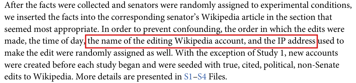
The editing account and the IP address were not randomly assigned in every study: IP addresses were randomized from Study 2 on, and after its first day Study 1 used a single account.

“Implementation on Wikipedia”, p. 3 (PDF p. 3), second and third sentences

As printed

In order to prevent confounding, the order in which the edits were made, the time of day, the name of the editing Wikipedia account, and the IP address used to make the edit were randomly assigned as well. With the exception of Study 1, new accounts were created before each study began and were seeded with true, cited, political, non-Senate edits to Wikipedia. More details are presented in S1–S4 Files.

The problem

The supplements state three exceptions that the summary omits. S2 File says that the IP address was “only introduced beginning in Study 2”. S1 File says that after the first day of Study 1, “All subsequent edits were made from the same account, veto118”, an account that “was randomly assigned to be the first account”. S4 and S5 Files say that the ten locked pages were edited from accounts that had “already been used to make edits in previous rounds of this experiment”. Note that reusing accounts does not contradict the statement that new accounts were created.

Evidence a check of the printed page

The evidence is a check of the page against the text of S1, S2, S4 and S5 Files.

What survives

The supplements disclose the exceptions, and no estimate depends on the summary. The assignment of valence and citation, the survival times and every reported estimate are unchanged. The wording alone does not show that any estimate is biased.

Corrected

In order to prevent confounding, the order in which the edits were made and the time of day were randomly assigned as well. IP addresses were randomly assigned beginning in Study 2. Accounts were initially randomly assigned; after the first day’s edits in Study 1, all subsequent edits used veto118, the account randomly assigned to be first. With the exception of Study 1, new accounts were created before each study began and were seeded with true, cited, political, non-Senate edits to Wikipedia; previously used, autoconfirmed accounts were used for locked pages in Study 4 and the concluding Study 5. More details are presented in S1–S5 Files.

Crop of the seven-line paragraph 'Implementation on Wikipedia'. A red box marks 'the name of the editing Wikipedia account, and the IP address' in the sentence 'In order to prevent confounding, the order in which the edits were made, the time of day, the name of the editing Wikipedia account, and the IP address used to make the edit were randomly assigned as well'.
“Implementation on Wikipedia”, p. 3 (PDF p. 3). The marked words are the two items whose random assignment did not hold in every study.

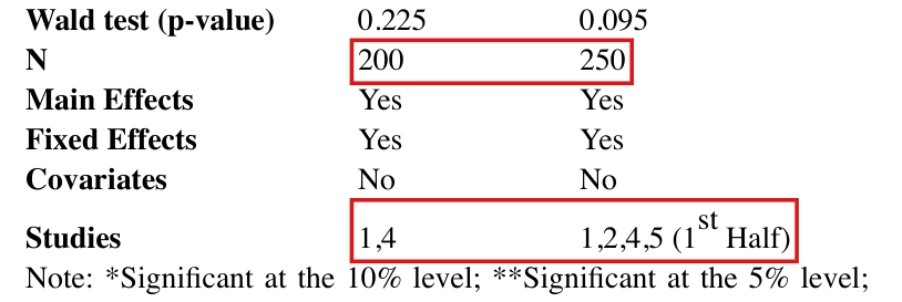
The entries of S9 Table B were estimated on 300 edits (Studies 1, 2, 4) and 400 edits (Studies 1, 2, 4, 5), not on the 200 and 250 edits that its rows “N” and “Studies” state.

S9 File, Table B (“Covariates as Moderators of Cited Edits from Cox Regressions”), rows “N” and “Studies”; the table is cited on p. 5 (PDF p. 5) of the article. The S9 File is a Word document without page numbers.

As printed
S9 File, Table B, last rows.
Column 1Column 2
Wald test (p-value)0.2250.095
N200250
Main EffectsYesYes
Fixed EffectsYesYes
CovariatesNoNo
Studies1,41,2,4,5 (1st Half)
The problem

The rows “N” and “Studies” describe the sample of each regression, and neither column is described correctly. The commands in the replication files restrict the first regression to Studies 1, 2 and 4 (300 edits) and the second to Studies 1, 2, 4 and all of Study 5 (400 edits). The second entry of the row “Studies” is also inconsistent with its own “N”, since Studies 1, 2, 4 and the first half of Study 5 contain 350 edits.

Evidence a recalculation from the source

The evidence is a recalculation from the replication files. On 300 and 400 edits, the fits reproduce all sixteen printed hazard ratios, all sixteen standard errors and both joint pp-values to three decimals. On the 200 and 250 edits in which citation was randomized (Studies 1 and 4, and these two with the first half of Study 5), the same model has joint pp-values 0.527 and 0.311. The interaction with influence then loses its marker, and the interaction with length of incumbency is significant at 5% and not at 1%.

What survives

If the two rows are corrected, the estimates, standard errors and tests in the table are unchanged. The main text (p. 5) cites the table for the statement that there is no systematic evidence that other variables moderate the effect of citations, and this statement is not weakened under either repair.

Corrected
S9 File, Table B, last rows, with the samples of the printed estimates.
Column 1Column 2
Wald test (p-value)0.2250.095
N300400
Main EffectsYesYes
Fixed EffectsYesYes
CovariatesNoNo
Studies1,2,41,2,4,5

Alternatively, the table may report the samples in which citation was randomized. The rows then read N = 200 and 250 and Studies “1,4” and “1,4,5 (1st Half)”, every hazard ratio, standard error and marker is replaced by its value on those samples, and the joint pp-values are 0.5274 and 0.3110.

The last six rows of a regression table with two columns of entries: Wald test (p-value) 0.225 and 0.095; N 200 and 250; Main Effects Yes, Yes; Fixed Effects Yes, Yes; Covariates No, No; Studies 1,4 and 1,2,4,5 (1st Half). Red boxes mark the two entries of the row N and the two entries of the row Studies.
S9 File, Table B, last rows and the first line of the note, in a rendering of the published Word file. The marked rows state 200 and 250 edits and the Studies “1,4” and “1,2,4,5 (1st Half)”.

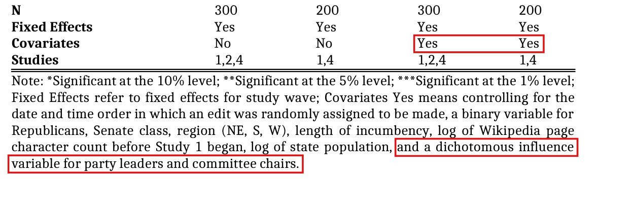
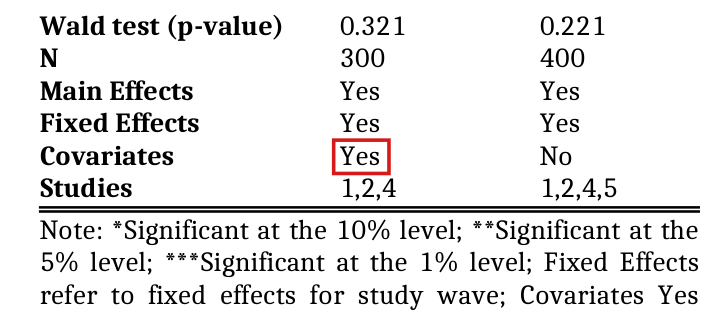
The note to the table of the S8 File lists a control for influence that its two adjusted models do not contain, and the first column of S9 Table A is marked “Covariates Yes” although its two columns fit the same specification and differ only in the studies included.

S8 File, row “Covariates” and note of the table; S9 File, Table A, row “Covariates”; S6 File, note to Table D. The supplementary files are Word documents without page numbers; they are listed on p. 6 (PDF p. 6) of the article, and the main text cites the S8 File on p. 5.

As printed

S8 File, note to the table: “Covariates Yes means controlling for the date and time order in which an edit was randomly assigned to be made, a binary variable for Republicans, Senate class, region (NE, S, W), length of incumbency, log of Wikipedia page character count before Study 1 began, log of state population, and a dichotomous influence variable for party leaders and committee chairs.”

S9 File, Table A, last rows.
Column 1Column 2
N300400
Main EffectsYesYes
Fixed EffectsYesYes
CovariatesYesNo
Studies1,2,41,2,4,5

S6 File, note to Table D: “****Date of entry and hour of entry removed to avoid convergence issues”.

The problem

In the S8 File, columns 3 and 4 are marked “Covariates Yes”, and the note says that this includes the influence variable. The commands in the replication files for these two columns do not contain that variable, and the printed entries reproduce without it and not with it. In S9 Table A, the note repeats this definition, and the row “Covariates” marks the first column “Yes” and the second “No”. The two commands have the same terms: the interactions of “Positive” with the moderators, the main effects of the moderators and indicators for study wave. Neither command adds the date of entry, the hour of entry or Senate class, and the columns differ only in the studies included. The note to S6 Table D defines a marker of four stars that no entry of that table carries. Since Table D is labelled as unadjusted and its command agrees with the label, this definition is superfluous and not false.

Evidence a recalculation from the source

The evidence is a recalculation from the replication files. The corrected descriptions of the entry-time and incumbency variables follow P041-E003 and P041-E004. Without the influence variable, the two adjusted models of the S8 File reproduce the six printed hazard ratios 0.574, 1.557, 0.783 and 0.507, 0.323, 2.146. With it, I obtain 0.580, 1.538, 0.774 and 0.515, 0.294, 2.237. The two specifications of S9 Table A, fitted to 300 and 400 edits, reproduce all sixteen printed hazard ratios of the interactions.

What survives

The reproduced hazard ratios are unchanged, and only the notes and the flag change. The interaction between citation and an upcoming election that the main text reports as 0.32 (p. 5) is the entry 0.323 of the S8 File, fitted without the influence variable; with that variable the interaction is 0.294 with p<0.001p<0.001.

Corrected

S8 File, note to the table, describing the models as fitted: “Covariates Yes means controlling for date of entry and seconds within the entry minute, a binary variable for Republicans, Senate class, region (NE, S, W), first-election year, log of Wikipedia page character count before Study 1 began, and log of state population.”

S9 File, Table A, row “Covariates”: No in both columns. The note may add that both models include the main effects of Republican status, influence, region, first-election year, log page character count and log state population, the interactions of “Positive” with each of them, and indicators for study wave; that neither model adds controls for the date of entry, the hour of entry or Senate class; and that the columns differ in the studies included.

S6 File, note to Table D: the clause “****Date of entry and hour of entry removed to avoid convergence issues” is deleted.

The last four rows of a regression table with four columns: N 300, 200, 300, 200; Fixed Effects Yes in all columns; Covariates No, No, Yes, Yes; Studies 1,2,4, then 1,4, then 1,2,4, then 1,4. Below is the note of the table. Red boxes mark the two entries 'Yes' of the row Covariates in columns 3 and 4, and the last clause of the note, 'and a dichotomous influence variable for party leaders and committee chairs.'
S8 File, last rows of the table and its note, in a rendering of the published Word file. The marked flags call columns 3 and 4 covariate-adjusted, and the marked clause of the note lists the influence variable among the covariates.
The last six rows of a regression table with two columns: Wald test (p-value) 0.321 and 0.221; N 300 and 400; Main Effects Yes, Yes; Fixed Effects Yes, Yes; Covariates Yes, No; Studies 1,2,4 and 1,2,4,5. A red box marks the entry 'Yes' of the row Covariates in the first column. Three lines of the note follow.
S9 File, Table A, last rows and the start of its note, in a rendering of the published Word file. The marked flag is “Yes” for “Covariates” in the first column.

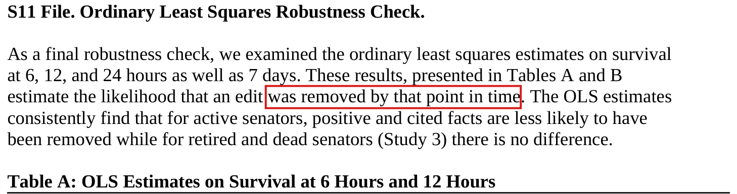
The outcome in Tables A and B of S11 File is survival beyond the stated time, not removal by it: read “survived beyond that point in time”.

S11 File, first paragraph, second sentence; cited from p. 4 (PDF p. 4), “further robustness checks are presented in Tables A and B in S11 File”

See also under Formal statements (Lean): P041-T9

As printed

These results, presented in Tables A and B estimate the likelihood that an edit was removed by that point in time.

The problem

The two tables are titled “OLS Estimates on Survival”. They regress an indicator that the fact was still present after 6, 12 or 24 hours or 7 days, and the printed slopes have the signs of that outcome. The sentence calls the outcome removal, for which every slope would have the opposite sign. The paragraph opens by naming survival, and the sentence that follows interprets the slopes correctly. The intended meaning can be recovered from them. The Harvard Dataverse copy (version 1.0) of the do-file codes the four outcomes as survival. The Yale Dataverse copy (version 2.0) codes them as removal by the stated time, and returns every slope with the sign opposite to the printed one.

Evidence a recalculation from the source

The evidence is an exact recalculation from the replication data. Let HiH_i be the duration of fact ii in hours and Si(h)=1{Hi>h}S_i(h)=\mathbf{1}\{H_i>h\}. With the outcome Si(h)S_i(h), all twelve printed slopes of the treatment indicators are reproduced to three decimals. For example, the six-hour slope for positive facts in Studies 1, 2 and 4 is 17/15017/150, printed as 0.113. The removal indicator is Ri(h)=1−Si(h)R_i(h)=1-S_i(h). Since each regression has an intercept, I have

β^R=e0−β^S,\widehat\beta_R=e_0-\widehat\beta_S,

for the two vectors of coefficients, where e0e_0 is the coordinate vector of the intercept. Every slope changes sign (−17/150-17/150 in the example), the residuals change sign, and the robust covariance matrix is the same.

What survives

All twelve printed slopes and their interpretation stand, and no coefficient changes. The Cox models, the Kaplan–Meier curves and Fig 1 use the duration and the failure indicator, not these four outcomes. The Yale copy of the do-file reproduces the printed signs once the coding of lines 147–154 of the Harvard copy is restored. That coding sets each of hour6, hour12, hour24 and day7 to 1, and replaces it by 0 when hours_alive is at or below the stated time.

Corrected

These results, presented in Tables A and B, estimate the likelihood that an edit survived beyond that point in time.

The heading S11 File, Ordinary Least Squares Robustness Check, a paragraph of five lines, and the title Table A: OLS Estimates on Survival at 6 Hours and 12 Hours. A red rectangle marks the words was removed by that point in time in the third line of the paragraph.
S11 File, first paragraph, on the first page of the supplement as rendered from the published Word file. The words “was removed by that point in time” are marked; the title of Table A below them says “Survival”.

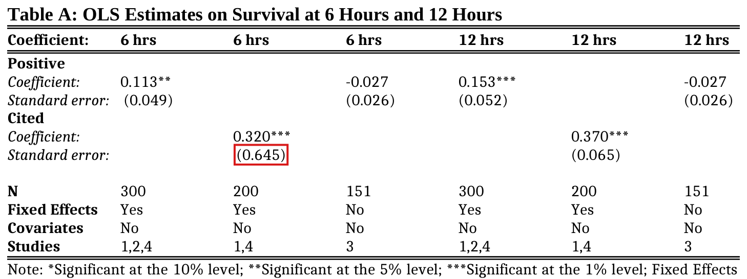
The standard error of the citation coefficient at six hours in Table A of S11 File is 0.064, not 0.645.

S11 File, Table A, column 2 (6 hrs; N=200N=200; Studies 1,4), standard error of “Cited”; cited from p. 4 (PDF p. 4)

See also under Formal statements (Lean): P041-T7

As printed
Table A: OLS Estimates on Survival at 6 Hours and 12 Hours
Coefficient:6 hrs
Cited
Coefficient:0.320***
Standard error:(0.645)
The problem

The printed standard error is about ten times too large. A coefficient of 0.320 with a standard error of 0.645 has t=64/129≈0.496t=64/129\approx0.496 and a two-sided pp of about 0.62, which contradicts the three stars printed beside the coefficient. The standard errors of the same coefficient at 12 hours, 24 hours and 7 days are printed as 0.065, 0.062 and 0.053.

Evidence a recalculation from the source

The evidence is a recalculation from the replication data in exact arithmetic. I regress the indicator of survival beyond six hours on an intercept, the citation indicator and an indicator for Study 4, in Studies 1 and 4. The regression has n=200n=200 and k=3k=3, and its citation coefficient is 8/25=0.3208/25=0.320. Each of the four cells of study by citation holds 50 facts, and the sum of squared residuals is 2047/502047/50. The HC1 variance of the citation coefficient is

200197⋅110000⋅204750=2047492500,\frac{200}{197}\cdot\frac{1}{10000}\cdot\frac{2047}{50}=\frac{2047}{492500},

and taking the square root, I find the standard error 2047/492500=0.0644697…\sqrt{2047/492500}=0.0644697\ldots, which rounds to 0.064. The tt statistic is then 4.96, with p≈1.5×10⁻⁶p\approx1.5\times10^{-6} on 197 degrees of freedom, in agreement with the three stars.

What survives

The coefficient 0.320 and its three stars stand. The recalculated standard errors at 12 hours, 24 hours and 7 days match their printed cells, and no other calculation uses this cell.

Corrected
Table A: OLS Estimates on Survival at 6 Hours and 12 Hours
Coefficient:6 hrs
Cited
Coefficient:0.320***
Standard error:(0.064)
Table A, OLS Estimates on Survival at 6 Hours and 12 Hours, with six columns. In the second column the coefficient for Cited is 0.320 with three stars, and a red rectangle marks the standard error (0.645) printed below it. The corresponding 12-hour entry in the fifth column is 0.370 with three stars and standard error (0.065).
S11 File, Table A, on the first page of the supplement as rendered from the published Word file. The standard error (0.645) of the six-hour coefficient for “Cited” is marked; the entry to its right, at 12 hours, is (0.065).

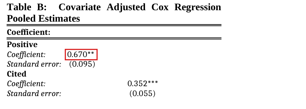
Four significance markers are one level off: “Positive” in S6 Table B should carry ***, the two entries for Study 5 in S6 Table E should carry **, and “Positive X NE Region” in the first column of S9 Table A should carry ** in place of ***.

S6 File, Table B (row “Positive”) and Table E (columns for Study 5); S9 File, Table A (row “Positive X NE Region”, first column). The supplementary files are Word documents without page numbers; they are listed on p. 6 (PDF p. 6) of the article.

See also under Formal statements (Lean): P041-T8

As printed

S6 File, Table B, “Positive”: 0.670** (0.095).

S6 File, Table E, “Cited”, Study 5 (1st Half): 0.480* (0.174); “Positive”, Study 5 (2nd Half): 0.274* (0.162).

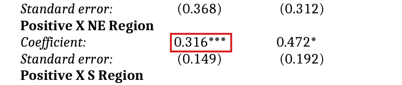
S9 File, Table A, “Positive X NE Region”, first column: 0.316*** (0.149).

Note to each table: “*Significant at the 10% level; **Significant at the 5% level; ***Significant at the 1% level”.

The problem

The tables print hazard ratios with standard errors on the scale of the hazard ratio, and their notes assign one star to the 10% level, two to the 5% level and three to the 1% level. For the four entries above, the printed marker is not the one that the printed hazard ratio and standard error imply. Three markers understate the level of significance. The fourth, in S9 Table A, claims significance at 1% for an interaction that is significant at 5%.

Evidence a recalculation from the source

The evidence is a calculation from the printed numbers and a recalculation from the replication files. For a printed hazard ratio H^\widehat{H} with standard error ss, the Wald statistic for the log hazard ratio and its two-sided pp-value are

z=log⁡H^s/H^,p=2 Φ(−∣z∣),z=\frac{\log \widehat{H}}{s/\widehat{H}},\qquad p=2\,\Phi(-|z|),

where Φ\Phi is the standard normal distribution function. The table below lists zz and pp at the printed values, bounds on pp over all hazard ratios and standard errors that round to the printed values, and the pp-value when the same model is fitted to the replication files. In every row these bounds lie on one side of the thresholds 0.01 and 0.05, so that rounding cannot account for the printed marker.

The four entries: the printed hazard ratio with its marker and standard error, the Wald statistic and pp-value that these give, and the marker that follows from the note of the tables. “S6 B” is Table B of the S6 File, and “5 (1st Half)” is the first half of Study 5; the entry of S9 Table A is in its first column.
EntryPrintedzzppBounds on ppRefit ppMarker
S6 B, Positive0.670** (0.095)−2.82-2.820.00470.0044–0.00510.0045***
S6 E, Cited, 5 (1st Half)0.480* (0.174)−2.02-2.020.04290.0418–0.04400.0434**
S6 E, Positive, 5 (2nd Half)0.274* (0.162)−2.19-2.190.02850.0276–0.02960.0285**
S9 A, Positive X NE Region0.316*** (0.149)−2.44-2.440.01460.0139–0.01520.0144**
What survives

The four estimates and their standard errors are unchanged. The joint tests 0.321 and 0.221 of S9 Table A are also unchanged. The correction leaves in place the statement of the main text that there is no systematic evidence of moderation by covariates. The interaction with the Northeast region remains significant at 5%.

Corrected

S6 File, Table B, “Positive”: 0.670*** (0.095).

S6 File, Table E, “Cited”, Study 5 (1st Half): 0.480** (0.174); “Positive”, Study 5 (2nd Half): 0.274** (0.162).

S9 File, Table A, “Positive X NE Region”, first column: 0.316** (0.149).

The top of a regression table titled 'Table B: Covariate Adjusted Cox Regression Pooled Estimates'. Under 'Positive', the coefficient 0.670** with standard error (0.095); under 'Cited', the coefficient 0.352*** with standard error (0.055). A red box marks 0.670**.
S6 File, Table B, in a rendering of the published Word file. The marked entry, for “Positive”, carries two stars.
A regression table titled 'Table E: Study by Study Cox Regression Estimates, with Covariate Adjustment', with five columns for Studies 1, 2, 4, 5 (1st Half) and 5 (2nd Half). Row Positive: 0.532***, 0.574, 0.753, 0.387***, 0.274*, with standard errors (0.108), (0.220), (0.200), (0.139), (0.162). Row Cited: 0.455***, blank, 0.239***, 0.480*, blank, with standard errors (0.090), (0.068), (0.174). Red boxes mark 0.274* in the last column and 0.480* in the fourth column.
S6 File, Table E, in a rendering of the published Word file. The marked entries are “Positive” for Study 5 (2nd Half) and “Cited” for Study 5 (1st Half), each with one star. The first line of the image is the end of the note to Table D.
Five rows of a regression table with two columns of entries. Under 'Positive X NE Region', the coefficients 0.316*** and 0.472* with standard errors (0.149) and (0.192). A red box marks 0.316***.
S9 File, Table A, rows around “Positive X NE Region”, in a rendering of the published Word file. The marked entry in the first column carries three stars.

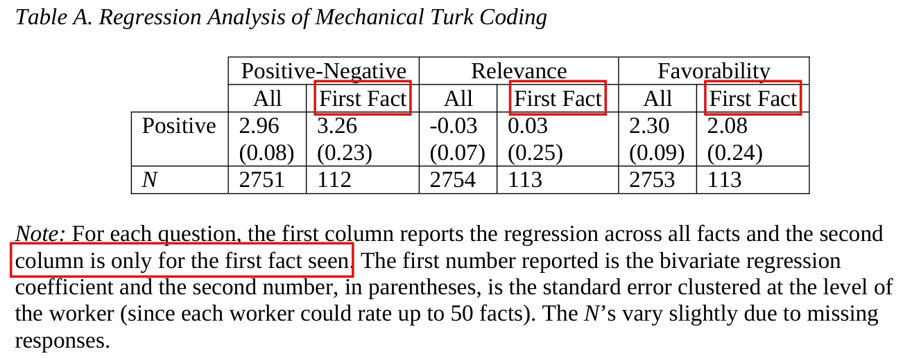
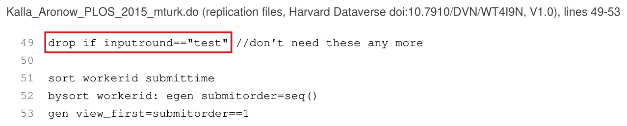
The “First Fact” columns of S12 Table A use each worker’s first substantive fact after the quality-control items have been dropped; seven of the 113 workers had already completed a quality-control item.

S12 File, Results, paragraph introducing Table A; Table A, “First Fact” columns and note (Word supplement, no fixed pagination); replication program Kalla_Aronow_PLOS_2015_mturk.do, lines 49–53

As printed

As an additional robustness check designed to guard against any desirability bias and learning that may occur as Mechanical Turk workers rate up to 50 of these facts, we produce the same regression using only the first randomly-assigned fact that each worker saw. The results are substantively the same.

Table A, “First Fact” columns: Positive-Negative, 3.263.26 (0.23)(0.23), N=112N=112; Relevance, 0.030.03 (0.25)(0.25), N=113N=113; Favorability, 2.082.08 (0.24)(0.24), N=113N=113.

Table A, note: For each question, the first column reports the regression across all facts and the second column is only for the first fact seen.

Replication program, lines 49 and 51–53:

drop if inputround=="test"

sort workerid submittime

bysort workerid: egen submitorder=seq()

gen view_first=submitorder==1

The problem

S12 File counts the 49 quality-control items among the facts that a worker could be shown: facts were sampled “from the set of 551 facts included in the five studies, plus an additional 49 facts that were seeded as quality control”, up to 50 per worker. The program drops the quality-control items in line 49 and ranks the submissions of each worker afterwards, in lines 51–53. The variable view_first therefore marks each worker’s first submitted substantive fact. Seven of the 113 workers had completed a quality-control item before that fact. For these seven the selected fact is not the first that the worker saw, and the restriction does not exclude earlier exposure to an item, which is the purpose stated for it.

Evidence an exact counterexample

The evidence is an exact counterexample from the replication data, with a recalculation. One worker submitted a quality-control item at 01:51:28 GMT on 9 December 2014 and accepted the selected fact, a Study 4 fact about Ed Markey, at 01:51:35, seven seconds later. For the seven workers the gaps between the submission of the quality-control item and the acceptance of the selected fact are 7, 3, 1, 1, 13, 6620 and 30 seconds. All six printed regressions of Table A reproduce at the printed precision. The slope of a regression on a binary indicator is the difference of the two group means. Without the seven workers, I find that the three slopes are 1535/4591535/459, −7/351-7/351 and 2987/14042987/1404.

Table A, restricted columns: coefficient (standard error clustered by worker) and NN.
QuestionAs printedNNWithout the seven workersNN
Positive-Negative3.26 (0.23)1123.34 (0.24)105
Relevance0.03 (0.25)113−0.02-0.02 (0.23)106
Favorability2.08 (0.24)1132.13 (0.25)106

The times are those of accepted and submitted assignments and do not show what a worker viewed. One retained worker accepted four substantive facts in the same second, so the order of viewing cannot be established for every worker.

What survives

The six printed regressions are correct for the samples that the program selects. Without the seven workers the pattern is the same: large positive differences for the positive-negative question and for favorability, and a difference near zero for relevance. The columns for all responses and the Wikipedia analyses do not use this restriction.

Corrected

Either keep the printed numbers, head the restricted columns “First substantive response”, and replace the description of the sample and the note to the table by the following text.

We repeat the regressions using each worker’s first submitted substantive fact, after removing quality-control items. Seven workers had previously completed a quality-control item; the restriction therefore avoids prior substantive responses but does not exclude prior quality-control exposure.

Or restrict the sample to the workers whose first recorded assignment, quality-control items included, was substantive, and replace the three restricted columns by 3.343.34 (0.24)(0.24), N=105N=105; −0.02-0.02 (0.23)(0.23), N=106N=106; and 2.132.13 (0.25)(0.25), N=106N=106. The text should then say that the order is that of accepted and submitted assignments, since no log of views exists.

Crop of the last four lines of the paragraph and the title of Table A. Red boxes mark 'using only the first' at the end of one line and 'randomly-assigned fact that each worker saw' at the start of the next.
S12 File, paragraph introducing Table A, from a rendering of the published Word file (the supplement has no fixed page numbers). The marked words describe the restricted sample.
Crop of Table A, 'Regression Analysis of Mechanical Turk Coding', and its note. Red boxes mark the three column heads 'First Fact', under Positive-Negative (3.26, standard error 0.23, N 112), Relevance (0.03, 0.25, 113) and Favorability (2.08, 0.24, 113), and the words 'column is only for the first fact seen' in the note.
S12 File, Table A and its note, from the same rendering. The marked column heads and the marked words of the note label the restricted columns.
Listing of lines 49 to 53 of the Stata program for the Mechanical Turk data. A red box marks 'drop if inputround=="test"' in line 49. Lines 51 to 53 read 'sort workerid submittime', 'bysort workerid: egen submitorder=seq()' and 'gen view\_first=submitorder==1'.
Replication program Kalla_Aronow_PLOS_2015_mturk.do, lines 49–53, typeset from the file. The marked command removes the quality-control items before the submissions of each worker are ranked.

The labels stored in the three figures of the S12 File are malformed: “Negative” and “Positive” are stored with a digit in place of the letters “ti”, and the tick labels have a percent sign in place of a space.

S12 File, Figures A–C (images embedded in a Word document without page numbers); the S12 File is listed on p. 6 (PDF p. 6) of the article

As printed
Text stored in the three figures of the S12 File.
FigureGroup labelsTick labels of two words
ANega2ve, Posi2veVery%Neg, Somewhat%Neg, Somewhat%Pos, Very%Pos
BNega3ve, Posi3veVery%Irr, Somewhat%Irr, Somewhat%Rel, Very%Rel
CNega5ve, Posi5veVery%Unfav, Somewhat%Unfav, Somewhat%Fav, Very%Fav
The problem

Each figure of the S12 File is an image embedded in the Word document, and the image stores its labels as text. In all three figures this text is malformed. The commands in the replication files that draw the figures contain the intended labels: “Negative” and “Positive” for the two groups, and tick labels such as “Very Neg” and “Somewhat Pos”.

Evidence a check of the printed page

The evidence is a check of the source file. I read the text that is stored in the three images embedded in the file, which consists of ordinary characters in the font Calibri. I did not check how the labels appear in Word with the original fonts.

What survives

No number depends on the labels, and the two groups and the response scale keep their intended meaning.

Corrected

Figures A–C are drawn again from the same data, with the group labels “Negative” and “Positive” and with spaces in the tick labels: “Very Neg”, “Somewhat Neg”, “Somewhat Pos” and “Very Pos” in Figure A, “Very Irr”, “Somewhat Irr”, “Somewhat Rel” and “Very Rel” in Figure B, and “Very Unfav”, “Somewhat Unfav”, “Somewhat Fav” and “Very Fav” in Figure C.

A box plot with two groups on the horizontal axis and seven tick labels, set at an angle, on the vertical axis. Red boxes mark the two group labels, which read 'Nega2ve' and 'Posi2ve', and the top tick label, in which a percent sign is printed over the gap between 'Very' and 'Pos'. From top to bottom, the other tick labels are Pos, Somewhat Pos, Neither, Somewhat Neg, Neg and Very Neg, and each label of two words has a percent sign in place of its space.
Figure A of the S12 File, in an earlier rendering of the embedded image. The marked group labels read “Nega2ve” and “Posi2ve”, and in the marked tick label a percent sign stands between “Very” and “Pos”. How the figure appears in Word with its original fonts was not checked.

Five slips of a word or label: read “far” for “fare”, “accounts” for “pages” and “effect of” for “effect if”, and in the codebook read Study 4 for Study 5 in the entry for the pre-election order and “character count” for “count” in the entry for page length.

Fig 1 caption, p. 4 (PDF p. 4), last sentence; S3 File, “Description of implementation”, last paragraph; S8 File, opening sentence; replication codebook, entries treatment_pre_order and pagechar

As printed
  • Fig 1 caption: “Results show that among active senators, negative facts are fare more likely to be removed more quickly than positive facts.”
  • S3 File: “We created 5 Wikipedia pages and made around 20 political, non-Senate edits using these accounts before beginning the experiment.”
  • S8 File: “Investigates whether Senate class is a moderator of the effect if positive and cited edits.”
  • Codebook: “treatment_pre_order: Order in which edits were made in Study 5, pre-election.”
  • Codebook: “pagechar: Senator’s Wikipedia page count before experiment began.”
The problem

The caption and S8 File contain misprints. The sentence of S3 File concerns the accounts created to reach autoconfirmed status and itself continues “using these accounts”. S2 File describes the same step as creating five Wikipedia accounts. The pre-election study is Study 4 (30–31 October 2014), and Study 5 followed the election (6–7 November 2014). The variable pagechar is the length of the page in characters, as p. 4 and the notes to the supplementary tables say.

Evidence a recalculation from the source

The evidence is a check of the page, the supplements and the codebook, and a recalculation from the replication data. In the data, treatment_pre_order is missing in Studies 1 to 3, is filled for all 100 Study 4 records, and is copied in the same order into the matching 100 Study 5 records. The values of pagechar range from 26686 to 631299.

What survives

These five wording changes do not alter any number or fitted result.

Corrected
  • Fig 1 caption: “Results show that among active senators, negative facts are far more likely to be removed more quickly than positive facts.”
  • S3 File: “We created 5 Wikipedia accounts and made around 20 political, non-Senate edits using these accounts before beginning the experiment.”
  • S8 File: “Investigates whether Senate class is a moderator of the effect of positive and cited edits.”
  • Codebook: “treatment_pre_order: Order in which edits were made in Study 4, pre-election (also carried into the corresponding Study 5 records).”
  • Codebook: “pagechar: Senator’s Wikipedia page character count before the experiment began.”
The three-line caption of Figure 1. A red rectangle marks the word fare in the sentence, Results show that among active senators, negative facts are fare more likely to be removed more quickly than positive facts.
Fig 1 caption, p. 4 (PDF p. 4), with the word “fare” marked in the last sentence.
Four lines of text. A red rectangle marks the word pages in the sentence, We created 5 Wikipedia pages and made around 20 political, non-Senate edits using these accounts before beginning the experiment.
S3 File, “Description of implementation”, last paragraph, on the single page of the supplement as rendered from the published Word file. The word “pages” is marked; the next line continues “using these accounts”.
Three lines of bold text beginning, S8 File. Investigates whether Senate class is a moderator of the effect if positive and cited edits. A red rectangle marks the word if at the end of the first line.
S8 File, opening sentence, on the single page of the supplement as rendered from the published Word file, with the word “if” marked.
Eight lines of the codebook in typewriter type, from committeechair to treatment_pre_order. Red rectangles mark the words page count in the entry, pagechar: Senator's Wikipedia page count before experiment began, and the words Study 5 in the entry, treatment_pre_order: Order in which edits were made in Study 5, pre-election.
Codebook of the replication files (PDF p. 1), entries pagechar and treatment_pre_order, with “page count” and “Study 5” marked.

In the plotting script, each survival curve should be extended to the 250-hour boundary only when the curve ends before 250 hours, and at its last survival level; as written, the loops draw a segment at survival zero beyond 250 hours, which the published Fig 1 does not show.

Fig 1, p. 4 (PDF p. 4), right-hand edge of the three panels; R plotting script of the replication files, lines 28 and 34–37, with the same loop at lines 43–46 and 51–54 and in the loops for Figure A of S6 File

As printed

maxtime <- 250

for (i in 1:length(fit1$strata)) { #number of curves

temp <- fit1[i]

lines(c(max(temp$time), maxtime), rep(min(temp$surv),2),

col=plot_colors[i],lty=plot_lty[i])

}

The problem

After each panel is plotted, a loop extends every curve to the display limit of 250 hours. The extension is meant for a curve whose fit stops before 250 hours, but the loop has no such condition. It uses the final fitted survival level, which need not be the level at 250 hours. For the eight curves of Fig 1 the fit ends at 3463.58037 hours with survival zero. This is the time that the script assigns to facts that were never removed (P041-N002). The loop draws a segment at survival zero from 3463.58037 hours back to 250 hours. With R’s default axis style, xaxs="r", the horizontal range 0 to 250 is widened to −10-10 to 260, and the part of the segment between 250 and 260 hours appears inside each panel. The published Fig 1 stops at 250 hours and shows no such segment.

Evidence a recalculation from the source

The evidence is a recalculation from the replication files and a check of the page. I ran the supplied plotting code with R’s default axes and recorded the coordinates of each extension. For all eight curves the extension runs from 3463.58037 hours to 250 hours at survival zero. The render shows a zero-level segment to the right of 250 hours in each panel. A second render, with the extension drawn only when max(temp$time) < maxtime and with xaxs="i", shows none. On the published page, viewed at 220 dpi, there is no mark at survival zero at the right-hand edge of any panel.

What survives

The published Fig 1 and the survival curves it shows over 0 to 250 hours are unaffected. Only a new render of the supplied script with default axes shows the extra segments. The same loop, without a condition, draws Figure A of S6 File.

Corrected

maxtime <- 250

for (i in 1:length(fit1$strata)) { #number of curves

temp <- fit1[i]

if (max(temp$time) < maxtime)

lines(c(max(temp$time), maxtime), rep(tail(temp$surv,1),2),

col=plot_colors[i],lty=plot_lty[i])

}

The same change applies to the loops for fit2 and fit3 and to the loops that draw Figure A of S6 File. To match the boundary of the published figure, each plot call also takes xaxs="i".

The three Kaplan-Meier panels of Figure 1, each with a horizontal axis from 0 to 250 hours and a vertical axis from 0 to 1, and the legend below them. A red rectangle encloses the lower right corner of each panel, where survival zero meets the 250-hour boundary. No curve or segment lies at survival zero inside the rectangles.
Fig 1, p. 4 (PDF p. 4), with the lower right corner of each panel marked. The published panels stop at 250 hours and carry no segment at survival zero there.
Two renders of Figure 1, one above the other, each with three panels of survival curves against hours from 0 to 250. In the upper render the horizontal axis runs a little past 250, and a short red segment at survival zero sits to the right of the 250 tick in each panel, circled in blue. In the lower render the axis stops at 250 and there is no segment at survival zero.
The plotting script run from the replication files. (a) As supplied, with R’s default axes: a segment at survival zero lies to the right of 250 hours in each panel (circled). (b) With the extension drawn only when a curve ends before 250 hours and with xaxs="i": no such segment.

The R script that draws the Kaplan–Meier figures builds its survival object without an event indicator, and the 257 facts that were never removed are entered as removals at an invented time of 3463.58 hours; line 14 should pass event=!wiki$dead.

Fig 1, p. 4 (PDF p. 4), and Figure A of S6 File; R plotting script of the replication files, lines 8–14

As printed

wiki$dead <- is.na(wiki$time_alive)

wiki$time_alive2 <- wiki$time_alive

wiki$time_alive2[wiki$dead] <- max(wiki$time_alive*2,na.rm=TRUE)

wiki$time_alive2[wiki$time_alive==0] <- 0.1

wiki$hours_alive <- wiki$time_alive2*2.77778e-7

wiki$survdata <- Surv(time=wiki$hours_alive)#,event=dead)

The problem

In R’s survival package, Surv called with a time and no event indicator gives every row status 1, an observed event. The outcome of the paper is the time until a fact is removed. In the data, 257 of the 551 facts were never removed: their time_alive is missing and removed is coded “NO”. Line 10 assigns these facts twice the largest recorded duration, that is, 3463.58 hours, and line 14 enters them as removals at that time. The fitted curve of any group that contains such facts then falls to zero at 3463.58 hours, where a Kaplan–Meier curve with these facts censored keeps its last level. The column dead is the missing-time indicator, not the removal indicator. It is TRUE for the facts that were never removed, and passing it as event would invert every status.

Evidence an exact counterexample

The evidence is an exact counterexample and a recalculation from the replication data. I take two records, one removed at raw time 3600000 and one never removed. The script assigns the second record the raw time 7200000, and with the conversion constant 2.77778×10−7=138889/5000000000002.77778\times10^{-7}=138889/500000000000 the two times are t1=1250001/1250000t_1=1250001/1250000 and t2=2t1t_2=2t_1 hours. The Kaplan–Meier estimator is

S^(t)=∏u≤t, d(u)>0n(u)−d(u)n(u),\widehat S(t)=\prod_{u\le t,\ d(u)>0}\frac{n(u)-d(u)}{n(u)},

where n(u)n(u) is the number of records with time at least uu and d(u)d(u) is the number of events at uu. At t1t_1 I have n=2n=2 and d=1d=1 whatever the status of the second record, which gives S^(t1)=1/2\widehat S(t_1)=1/2. With the statuses (1,1)(1,1) of the script, n(t2)=d(t2)=1n(t_2)=d(t_2)=1 and S^(t2)=0\widehat S(t_2)=0. With the statuses (1,0)(1,0), no factor is added at t2t_2 and S^(t2)=1/2\widehat S(t_2)=1/2.

In the data, the largest recorded duration is 6234439680 in raw units. The invented time is then 169120135296/48828125=3463.58037086208169120135296/48828125=3463.58037086208 hours, and all 551 statuses are 1. A fact that was never removed has time 3463.58>2503463.58>250 in the survival object of the script and in the repaired one, and every recorded removal is the same in both. For every u≤250u\le250 the two objects then have the same n(u)n(u) and d(u)d(u). This implies that the Kaplan–Meier products agree on [0,250][0,250]. In exact arithmetic on the data, the two products agree for all 26 fitted curves, 8 in Fig 1 and 18 in Figure A of S6 File. The table lists the curves of Fig 1.

Curves of Fig 1, as scripted and with the event indicator repaired. The value at 250 hours is the same in both cases. The last two columns give the value at the invented time of 3463.58 hours.
StudiesConditionNNNever removedS^(250)\widehat S(250)As scriptedRepaired
1 and 4Positive, cited511616/5116/51016/5116/51
1 and 4Positive, uncited4955/495/4905/495/49
1 and 4Negative, cited491010/4910/49010/4910/49
1 and 4Negative, uncited5131/171/1701/171/17
2Positive, cited50374/54/5037/5037/50
2Negative, cited503016/2516/2503/53/5
3Positive, cited756768/7568/75067/7567/75
3Negative, cited766473/7673/76016/1916/19
What survives

Every Kaplan–Meier value shown in Fig 1 and in Figure A of S6 File, which stop at 250 hours, is unchanged when only the event indicator is repaired. The Cox regressions, the regression tables and the counts at fixed times come from the Stata do-file and do not use the R object. The do-file sets dead to 1 for a recorded removal and declares it with stset hours_alive, failure(dead). The fitted curves beyond 250 hours and any summary of the full fit do change. The repair keeps the time that the script assigns to facts that were never removed. Whether that time matches the actual end of monitoring is a separate question, which this correction does not settle.

Corrected

wiki$survdata <- Surv(time=wiki$hours_alive, event=!wiki$dead)

Lines 8–13 are unchanged. The indicator is the negation of dead, since in this script dead is TRUE for a fact that was never removed.

The lower edge of the three panels of Figure 1, with horizontal axes labelled Hours and ticks from 0 to 250, the legend, and the caption. Red rectangles mark the tick label 250 of each panel and the caption title, Fig 1. Kaplan-Meier survival curves across all studies and all conditions.
Fig 1, p. 4 (PDF p. 4): the title of the caption and the last tick of each horizontal axis are marked. The panels stop at 250 hours; the removals that the script invents lie at 3463.58 hours, outside the figure.

The sentence cites Table A of S9 File and S10 File for eight moderators of the valence effect, but the test for Senate class is in S8 File, S10 File is not a moderation analysis, and no test for date or time of entry is reported: cite S8 File and Table A of S9 File, and remove date and time of entry from the list.

Results, “Survival of Positive and Negative Facts on Wikipedia”, last sentence of the first paragraph, p. 4 (PDF p. 4)

As printed

We find no systematic evidence that this effect is moderated by covariates (state population, Senate class, character count of page, geographic region, length of incumbency, political party, date of entry, and time of entry; see Table A in S9 File and S10 File), as specified in our registered pre-analysis plan.

The problem

Table A of S9 File reports interactions of the indicator for positive facts with party, influence, three regions, length of incumbency, log page length and log state population. It has no interaction with Senate class, date of entry or time of entry. S10 File regresses survival on covariates alone, with no valence indicator and no interaction, and therefore cannot test moderation. The one reported test of Senate class as a moderator of the valence effect is in S8 File, which the sentence does not cite. There Senate class is dichotomized as facing reelection in 2014, and the interaction is 1.750* (0.550) without covariates and 1.557 (0.485) with them. No supplement and neither copy of the do-file reports an interaction of valence with date or time of entry. These two variables enter only as additive controls.

Evidence a check of the printed page

The evidence is a check of the page against the twelve supplements and the replication do-files. I write the Cox model with interactions as h(t∣V,Z)=h0(t)exp⁡{βV+γ⊤Z+δ⊤(VZ)}h(t\mid V,Z)=h_0(t)\exp\{\beta V+\gamma^\top Z+\delta^\top(VZ)\}, where V=1V=1 for a positive fact and ZZ is the vector of covariates. Dividing the hazard of a positive fact by the hazard of a negative fact at Z=zZ=z, I find the hazard ratio exp⁡(β+δ⊤z)\exp(\beta+\delta^\top z). Moderation is a statement about δ\delta, and S10 File estimates only γ\gamma. The joint Wald tests of Table A in S9 File have p=0.321p=0.321 and p=0.221p=0.221. From the rounded entries of S8 File, the interaction with Senate class has p≈0.075p\approx0.075 without covariates and p≈0.155p\approx0.155 with them.

What survives

The analyses that are reported do not contradict the statement of no systematic evidence. The joint tests do not reject, and the interaction with Senate class is marginal only without covariates. The cited files do not document three of the eight listed moderators, and the corrected sentence covers six. The pooled valence estimates, the survival curves and the citation results do not depend on this sentence. I could not compare the sentence with the pre-analysis plan, which was not available.

Corrected

We find no systematic evidence that this effect is moderated by covariates (state population, Senate class dichotomized as facing reelection in 2014, character count of page, geographic region, length of incumbency, and political party; see S8 File and Table A in S9 File), as specified in our registered pre-analysis plan.

Date and time of entry may return to the list once their interactions with valence are reported. The covariate called length of incumbency is the year of first election (P041-E004).

Four lines of text beginning, We find no systematic evidence that this effect is moderated by covariates. Two red rectangles on the third line mark the words date of entry, and time of entry, and the citation see Table A in S9 File and S10 File.
Results, p. 4 (PDF p. 4): the last sentence of the first paragraph, with “date of entry, and time of entry” and the citation “see Table A in S9 File and S10 File” marked.

Random assignment of the order of the edits does not by itself ensure that speeding up Study 1, and converting the remaining uncited edits of Study 5 to cited ones, leave the comparisons unbiased.

S1 File and S5 File, “Description of implementation”, last sentence of each (Word supplements, no fixed pagination); the main text refers to S5 File on p. 3 (PDF p. 3)

See also under Formal statements (Lean): P041-T5, P041-T6, P041-T13

As printed

S1 File: Because other Wikipedia editors became suspicious of this account’s uncited edits and threatened to block the account, we sped up the implementation and finished implementing the experiment sooner than anticipated, on 15 July 2014. Because the order in which edits were made was randomly assigned, this does not bias our results.

S5 File: After implementing the first 50 edits on 6 November 2014, other Wikipedia editors became suspicious. We decided to convert all of the uncited edits in the remaining 50 edits to cited edits. Thus the first 50 edits had all four conditions while the last 50 edits only had positive or negative conditions, with all facts cited. Because the order in which edits were made was randomly assigned, this does not bias our results.

The problem

In each supplement, “this” refers to a change made after editors reacted to the uncited edits: the remaining edits of Study 1 were made faster, and the remaining uncited edits of Study 5 were made cited. Random order balances, in expectation, any pattern over the calendar that does not depend on the treatments. It does not cover the case that the supplements describe, in which the treatment of earlier edits (an uncited fact from the same account) changes how later edits are received or when they are made. In that case the comparison under the protocol that was carried out need not equal the comparison under the planned protocol, or the effect of an edit’s own treatment. Random order gives no guarantee here. To keep the assurance, one needs a further assumption that excludes such effects of earlier edits on later ones. An example is the assumption that the removal of an edit does not depend on the treatments and timing of the earlier edits from the account. The supplements state no such assumption, and the replication data do not identify the editors who removed the facts. This is a limit on the assurance; it does not show that any estimate is biased.

Evidence an exact counterexample

The evidence is an exact counterexample to the sufficiency of random order, with a recalculation of two sensitivity checks. I take four pages, two assigned a cited fact (C) and two an uncited fact (U), as in one block of Study 1, and let the 24 orders of insertion be equally likely. Suppose that an uncited edit starts a period in which every later insertion from the account is removed, whatever its own citation status, and that no other removals occur. This response is hypothetical and is not a description of the actual editors. On the planned, slow schedule the period ends before the next insertion, no fact is removed, and the difference DD between the removal rates of cited and uncited facts is 00. On the accelerated schedule, all remaining insertions fall inside the period that the first uncited edit starts. The edit at rank rr is then removed if and only if an earlier edit is uncited,

Yr=1{zs=U for some s<r},Y_r=\mathbf{1}\{z_s=\mathrm{U}\ \text{for some}\ s<r\},

where zsz_s is the type of the edit at rank ss. The outcome YrY_r does not depend on zrz_r, which implies that the effect of an edit’s own citation is zero. The six orders of types are equally likely.

The six equally likely orders of types on the accelerated schedule.
Types at ranks 1–4Removed at ranks 1–4Cited rateUncited rateDD
U U C C0 1 1 1111/21/21/21/2
U C U C0 1 1 1111/21/21/21/2
U C C U0 1 1 1111/21/21/21/2
C U U C0 0 1 11/21/21/21/200
C U C U0 0 1 11/21/21/21/200
C C U U0 0 0 1001/21/2−1/2-1/2

Averaging over the six orders, I obtain

E[D]=16(12+12+12+0+0−12)=16,\mathbb{E}[D]=\frac{1}{6}\Bigl(\frac12+\frac12+\frac12+0+0-\frac12\Bigr)=\frac16 ,

against 00 on the slow schedule, although the order is uniformly random and the citation has no effect of its own. With 100 pages, 50 cited and 50 uncited, the same construction has expected removal rates 50/5150/51 and 49/5049/50, and I find that E[D]=1/2550\mathbb{E}[D]=1/2550. This value shows that the expectation need not vanish. It is not an estimate of any bias in the paper. If the pattern of removals is fixed over the calendar and does not depend on the treatments, the same enumeration gives E[D]=0\mathbb{E}[D]=0.

The replication data show removals concentrated in time: in Study 1, 55 of the 93 removals fall between 19:28 and 20:39 on 15 July 2014, and all 36 facts inserted on that day were removed on that day. For the pooled comparison of positive and negative facts (Studies 1, 2 and 4), I re-estimated the Cox model in R. With robust standard errors computed without clustering, as in the replication program, the hazard ratio is 0.6290.629 and p=0.0013p=0.0013. With standard errors clustered by senator, I find p=0.0008p=0.0008. Without the 36 Study 1 edits of the last day, the hazard ratio is 0.6060.606 and p=0.0016p=0.0016.

What survives

The counts, the survival curves and the fitted coefficients are unchanged, and no numerical correction follows. The pooled difference between positive and negative facts remains under clustering by senator and without the last day of Study 1. These checks do not address an effect of earlier edits on later ones within an account. Study 1 enters both pooled analyses of the main text. Study 5 enters supplementary analyses and is excluded from the main-text pooled estimates. What is withdrawn is the unconditional assurance for Studies 1 and 5.

Corrected

S1 File and S5 File, in place of the marked sentence: Random assignment of the original order prevents deliberate ordering by treatment. It does not by itself rule out treatment-dependent account responses or effects of the adaptive changes.

If the comparisons are read as effects of an edit’s own treatment, the text should also state the protocol and the conditions of exposure to which they refer.

Crop of the four-line last paragraph of S1 File. Red boxes mark the sentence 'Because the order in which edits were made was randomly assigned, this does not bias our results.', which runs over the last two lines.
S1 File, “Description of implementation”, last paragraph, from a rendering of the published Word file (the supplement has no fixed page numbers). The marked sentence is the assurance.
Crop of the last five lines of S5 File. Red boxes mark the sentence 'Because the order in which edits were made was randomly assigned, this does not bias our results.', which runs over the last two lines.
S5 File, “Description of implementation”, end of the last paragraph, from a rendering of the published Word file. The marked sentence is the same assurance.

The six Fleiss kappas reported in S12 File do not show “fairly strong agreement”: the two for relevance are 0.04 and 0.08, and the largest of the six is 0.56.

S12 File, Results, second paragraph (Word supplement, no fixed pagination)

As printed

When we calculate the inter-rater reliability across the facts and five raters, we find fairly strong agreement. On the positive-negative question, the Fleiss’s kappa across all seven categories is 0.20 and 0.56 when collapsed to three categories. On the relevance question, the Fleiss’s kappa across all seven categories is 0.04 and 0.08 when collapsed to three categories. On the favorability question, the Fleiss’s kappa across all seven categories is 0.13 and 0.38 when collapsed to three categories.

The problem

The sentence summarizes the six kappas that follow it. A Fleiss kappa measures how far the raters agree on the exact category beyond the agreement expected from the pooled frequencies of the categories. For relevance the two values are 0.0360.036 and 0.0770.077: the raters agree in 25.2%25.2\% of pairs against a benchmark of 22.5%22.5\% with seven categories, and in 58.2%58.2\% against 54.7%54.7\% with three. As a summary that includes relevance, “fairly strong” overstates these values. The paper sets no threshold for the phrase, and the finding concerns the wording; the six numbers are correct.

Evidence a recalculation from the source

The evidence is a recalculation from the replication data, in exact arithmetic. There are 551 facts with five ratings each, and a missing rating is set to the midpoint 4, as in the replication program. Let PoP_o be the share of agreeing pairs of raters among the 55105510 pairs and Pe=∑jpj2P_e=\sum_j p_j^2, where pjp_j is the pooled share of category jj. The kappa is κ=(Po−Pe)/(1−Pe)\kappa=(P_o-P_e)/(1-P_e). For relevance with seven categories I obtain

Po=13915510,Pe=17049717590025,κ=42226311770108≈0.0359,P_o=\frac{1391}{5510},\qquad P_e=\frac{1704971}{7590025},\qquad \kappa=\frac{422263}{11770108}\approx0.0359 ,

and with three categories

Po=32075510,Pe=41540837590025,κ=5271196871884≈0.0767.P_o=\frac{3207}{5510},\qquad P_e=\frac{4154083}{7590025},\qquad \kappa=\frac{527119}{6871884}\approx0.0767 .

The six kappas are 0.2020.202 and 0.5590.559 for the positive-negative question, 0.0360.036 and 0.0770.077 for relevance, and 0.1340.134 and 0.3810.381 for favorability, and each rounds to the printed value.

What survives

The six kappas stand. The mean ratings separate the two kinds of facts: positive minus negative is 2.962.96 points for the positive-negative question and 2.302.30 for favorability, and −0.03-0.03 for relevance. The description of the facts as positive or negative rests on these means, and the analyses of survival do not use the ratings.

Corrected

Agreement varied by question and category resolution: it was greatest for valence after collapsing to three categories, while relevance showed little exact-category agreement beyond the marginal-frequency chance benchmark. On the positive-negative question, the Fleiss’s kappa across all seven categories is 0.20 and 0.56 when collapsed to three categories. On the relevance question, the Fleiss’s kappa across all seven categories is 0.04 and 0.08 when collapsed to three categories. On the favorability question, the Fleiss’s kappa across all seven categories is 0.13 and 0.38 when collapsed to three categories.

Crop of two paragraphs of S12 File. Red boxes mark 'fairly strong' at the end of one line and 'agreement' at the start of the next, in 'When we calculate the inter-rater reliability across the facts and five raters, we find fairly strong agreement'. The following sentences give the kappas 0.20 and 0.56, 0.04 and 0.08, 0.13 and 0.38.
S12 File, Results, first and second paragraphs, from a rendering of the published Word file (the supplement has no fixed page numbers). The marked words summarize the six kappas that follow.

Clarity notes

Imprecise or ambiguous wording whose intended meaning is correct; not an error.

S12 File detects no difference in mean relevance between positive and negative facts (−0.03-0.03, standard error 0.070.07); the sentence can be read as if equal relevance had been established at a significance level.

S12 File, Results, paragraph introducing Table A (Word supplement, no fixed pagination)

As printed

Consistent with the box-plots, we see that positive facts were perceived to be more positive, equally relevant, and more favorable at statistically significant levels.

Intended meaning

The phrase “at statistically significant levels” applies to the two differences that Table A shows to be significant, 2.962.96 (standard error 0.080.08) for the positive-negative question and 2.302.30 (0.09)(0.09) for favorability. For relevance the table shows −0.03-0.03 (0.07)(0.07), and the two mean ratings are 5.005.00 and 5.035.03, so “equally relevant” means that no difference in mean relevance was detected. Read in this way the sentence is correct. A test of a zero difference that does not reject is not a test of equivalence, and S12 File reports no equivalence margin or test.

Corrected

Consistent with the box-plots, positive facts were perceived as more positive and more favorable at statistically significant levels; no statistically detectable difference in mean relevance was found.

Crop of the eight-line paragraph that introduces Table A. Red boxes mark 'more positive,' at the end of one line and 'equally relevant, and more favorable at statistically significant levels' at the start of the next.
S12 File, paragraph introducing Table A, from a rendering of the published Word file (the supplement has no fixed page numbers). The marked words join “equally relevant” to “at statistically significant levels”.

The entries labelled “Coefficient:” in the Cox tables of S6–S10 Files are hazard ratios, and their standard errors are on the hazard-ratio scale.

S6–S10 Files, row label “Coefficient:” in every Cox table (for example S6 File, Table A); cited from p. 4 (PDF p. 4), “hazard ratio = 1.59”

As printed

Table A: Pooled Cox Regression Estimates
Coefficient:
Positive
Coefficient:0.629***
Standard error:(0.091)
Cited
Coefficient:0.429***
Standard error:(0.069)

Intended meaning

The entries are exponentiated Cox coefficients, that is, removal hazard ratios for the named condition against its reference, and the standard errors are on the same scale. For the row “Positive” of Table A in S6 File, the fitted coefficient on the log-hazard scale is −0.4637-0.4637. Its exponential is 0.629, and 0.629 times the robust standard error of the coefficient is 0.091. The main text prints the reciprocals: 1.59≈1/0.6291.59\approx1/0.629 on p. 4 for negative against positive facts, and 2.33≈1/0.4292.33\approx1/0.429 on p. 5 for uncited against cited facts. The supplements do not use the words “hazard ratio”, but the surrounding text and these reciprocals identify the intended scale.

Corrected

Table A: Pooled Cox Regression Estimates
Hazard ratio:
Positive
Hazard ratio:0.629***
Standard error of the hazard ratio:(0.091)
Cited
Hazard ratio:0.429***
Standard error of the hazard ratio:(0.069)

The same two labels replace “Coefficient:” and “Standard error:” in the other Cox tables of S6–S10 Files.

The top of Table A, Pooled Cox Regression Estimates. Red rectangles mark the word Coefficient in the header row and beside the entries 0.629 with three stars, for Positive, and 0.429 with three stars, for Cited. The standard errors 0.091 and 0.069 are printed in parentheses below.
S6 File, Table A, on the first page of the supplement as rendered from the published Word file. The label “Coefficient:” is marked in the header and in the rows “Positive” and “Cited”; the entries 0.629 and 0.429 are hazard ratios.

Formal statements (Lean)

Formal results: 9 whole; 2 restricted; 1 refuted; 1 omitted.

Coverage concerns the identified claim under its stated assumptions. A checked proof establishes the formal statement; correspondence to the published text was reviewed by AI. Repository access is currently required to open the source links.

Each result links to its current formal statement and proof. “Whole” covers the identified claim under its assumptions; “restricted” covers the stated narrower scope; “refuted” gives a counterexample to the identified assertion; “omitted” has no current theorem. Any named published theorem used as a premise remains an assumption. Browse the formal results for this work.

‘Replication on Wikipedia Pages of Dead and Retired Senators’, last two sentences (‘This suggests that the editorial bias cannot be explained by … Instead, our findings suggest the editorial bias is limited to active politicians’), and Discussion, first paragraph (‘suggesting that this bias is limited to the pages of active politicians and is not systemic to Wikipedia’): the inference from the Study 3 comparison to confinement of the bias; the witness is the validator's construction and is not in the paper

p. 5/8 (PDF p. 5); the claim recurs in the Abstract, p. 1/8 (PDF p. 1)

p. 5/8 (PDF p. 5); the claim recurs in the Abstract, p. 1/8 (PDF p. 1). The stipulated exponential countermodel has common non-null hazard ratios, exact unequal 12-hour contrasts, and positive binomial expressions at all four observed counts.

Historical component credits
  • Proved AronowAudit.P041.proportional_hazards Historical support retained; baseline fidelity: ok; manifest: used; used in Solution; The hazards are constant real numbers, so their ratio has no time dependence; no fitted population inference is credited to this lemma.
  • Proved AronowAudit.P041.exponential_survival_power_laws Historical support retained; baseline fidelity: ok; manifest: used; used in Solution; The larger domain is harmless; q>1 or negative t is treated only as an algebraic function identity, not a survival-probability assertion.
  • Proved AronowAudit.P041.twelve_hour_survival Historical support retained; baseline fidelity: ok; manifest: used; used in Solution; The extra q≥1 cases are algebraic extensions; on 0<q<1 the identity is exactly the target’s survival claim.
  • Proved AronowAudit.P041.binomial_count_positive Historical support retained; baseline fidelity: ok; manifest: used; used in Solution; This is the general auxiliary positivity lemma described by the row; it does not itself assert independence in the experiment.
  • Counterexample proved AronowAudit.P041.common_bias_countermodel Historical support retained; baseline fidelity: ok; manifest: used; used in Solution; This is an exact witness to the stated non-implication, not a refutation of the actual population-confinement hypothesis or a fitted significance analysis.

‘Replication on Wikipedia Pages of Dead and Retired Senators’, last two sentences, and Discussion, first paragraph, last sentence, as repaired by Sol: nondetection in Study 3 with an imprecise relative estimate, smaller early absolute contrasts, and no exclusion of a relative bias on former senators' pages

p. 5/8 (PDF p. 5); the tables used are S6 Table A (rendered p. 1) and S6 Table C (rendered p. 2)

p. 5/8 (PDF p. 5); the tables used are S6 Table A (rendered p. 1) and S6 Table C (rendered p. 2). The supplied rounded table entries give imprecise former-senator relative effects, smaller pooled early contrasts, and a countermodel to absence of relative bias.

Historical component credits
  • Proved AronowAudit.P041.corrected_former_nondetection Historical support retained; baseline fidelity: ok; manifest: used; used in Solution; The row covers the statistic bound, with the printed-pair p-value covered by R240-06.
  • Proved AronowAudit.P041.corrected_former_imprecision Historical support retained; baseline fidelity: ok; manifest: used; used in Solution; The target explicitly stipulates 1.96, so using 49/25 instead of the exact Gaussian quantile is faithful; the redundant active-SE restriction excludes no allowed four-tuple.
  • Proved AronowAudit.P041.corrected_between_relative_effects Historical support retained; baseline fidelity: ok; manifest: used; used in Solution; Independence is the target’s interpretation of the numerical standard-error formula, not an unproved independence conclusion in this scalar theorem.
  • Proved AronowAudit.P041.former_wald_endpoint_enclosures Historical support retained; baseline fidelity: ok; manifest: used; used in Solution; The row covers the quantitative endpoint enclosures, with the interval-membership claims covered separately by R240-08.
  • Proved AronowAudit.P041.observed_early_contrasts Historical support retained; baseline fidelity: ok; manifest: used; used in Solution; The count inputs are stipulated by the target; no archive extraction, timestamp authentication, or cited-only comparison is asserted.
  • Proved AronowAudit.P041.smaller_contrast_does_not_exclude_common_bias Historical support retained; baseline fidelity: ok; manifest: used; used in Solution; The exported existential is sufficient for the non-implication component; the exact numerical witness is additionally established by R240-02.
  • Proved AronowAudit.P041.Wave1.corrected_normal_p_approximations_proof Historical support retained; baseline fidelity: ok; manifest: used; used in Solution; The claimed p-values are approximations at the printed central pairs; the row is not assigned uniform normal-tail bounds over all rounding choices.

Abstract, ‘Negative facts are 36% more likely to be removed by Wikipedia editors than positive facts within 12 hours and 29% more likely within 3 days’, and ‘Effects of Citations on Survival’, ‘uncited (but true) facts are 64% more likely to be removed than cited facts within four hours’, as printed; the counts are the validators' recounts of the deposited data and are not printed in the paper

Abstract, p. 1/8 (PDF p. 1); ‘Effects of Citations on Survival’, sentence running from p. 4/8 to p. 5/8 (PDF pp. 4–5)

Abstract, p. 1/8 (PDF p. 1); ‘Effects of Citations on Survival’, sentence running from p. 4/8 to p. 5/8 (PDF pp. 4–5). The three printed directional percentages fail individually, while the symmetric percentages round as printed and strictly understate directional increases.

Historical component credits
  • Counterexample proved AronowAudit.P041.risk_percentages_counterexample Historical support retained; baseline fidelity: ok; manifest: used; used in Solution; The reference group and direction are exactly the printed wording’s natural reading fixed by the target; this does not refute the counts, qualitative direction, or Cox ratios.
  • Proved AronowAudit.P041.symmetric_understates_relative Historical support retained; baseline fidelity: ok; manifest: used; used in Solution; The scalar domain a>b>0 is exactly that in T3(iv), with no artificial probability upper bound.
  • Proved AronowAudit.P041.risk_measure_gaps Historical support retained; baseline fidelity: ok; manifest: used; used in Solution; Using counts rather than proportions leaves both measures unchanged when the two arms have equal size, as stipulated here.

Abstract, the sentence with ‘36%’ and ‘29%’, and ‘Effects of Citations on Survival’, the sentence with ‘64%’, as repaired by Sol: 44%, 33% and 94%, computed as relative increases in the proportion removed

Abstract, p. 1/8 (PDF p. 1); ‘Effects of Citations on Survival’, pp. 4/8–5/8 (PDF pp. 4–5)

Abstract, p. 1/8 (PDF p. 1); ‘Effects of Citations on Survival’, pp. 4/8–5/8 (PDF pp. 4–5). The supplied counts give the corrected directional percentages, the conditional 76-removal variant, and the symmetric alternative repair.

Historical component credits
  • Proved AronowAudit.P041.corrected_risk_percentages Historical support retained; baseline fidelity: ok; manifest: used; used in Solution; The conditional 76-count case is represented by evaluating the function at that distinct input; this neither asserts that 76 is the stored-duration count nor that a timestamp repair has occurred.

S1 File and S5 File, ‘Description of implementation’, last sentence of each (‘Because the order in which edits were made was randomly assigned, this does not bias our results’), as printed; the witness is the validator's construction and is not in the paper

S1 File, last paragraph (rendered p. 2); S5 File, last paragraph (rendered p. 2); the main article points to S5 on p. 3/8 (PDF p. 3)

S1 File, last paragraph (rendered p. 2); S5 File, last paragraph (rendered p. 2); the main article points to S5 on p. 3/8 (PDF p. 3). A uniformly balanced order with scrutiny gives zero direct effects and slow contrast but a positive accelerated expectation, with the full six-order table, general formula, size-50 instance, zero expected contrast for every fixed treatment-independent outcome pattern at every m >= 1, its four-rank example, and the independent-assignment boundary.

Historical component credits
  • Proved AronowAudit.P041.scrutiny_no_direct_effect Historical support retained; baseline fidelity: ok; manifest: used; used in Solution; The broader finite-length quantifier loses no target case. The record’s generic mention of unbalanced inputs as stronger is unnecessary for T5(i), whose own text already includes unbalanced sequences.
  • Proved AronowAudit.P041.slow_schedule_zero Historical support retained; baseline fidelity: ok; manifest: used; used in Solution; {'source': 'adjudication', 'decision': 'rejected', 'what': 'P041/P041_Order.lean:68 states that citationContrast m z (fun _ => 0) is zero for every m and every cited-rank subset. This matches T5(ii), which explicitly stipulates zero slow-schedule outcomes and concludes that the slow contrast is zero for every order; the clock mechanism is not an additional conclusion of this component. The m=0 extension uses totalized division, but every intended m≥1 case is retained and holds without division by zero, so the row is not vacuous or materially restricted.'}
  • Counterexample proved AronowAudit.P041.random_order_block_counterexample Historical support retained; baseline fidelity: ok; manifest: used; used in Solution; The witness refutes sufficiency of random order under the target’s explicit reading. It does not refute actual unbiasedness of the study’s Cox estimates or model the distinct Study 5 implementation change.
  • Proved AronowAudit.P041.Wave1.balanced_scrutiny_general_proof Historical support retained; baseline fidelity: ok; manifest: used; used in Solution; This row supplies T5(iv), not a standalone assertion about actual Wikipedia bias. The target explicitly stipulates the balanced type-sequence law, so no extra assignment restriction is imposed.
  • Proved AronowAudit.P041.compressed_scrutiny50_certificate Historical support retained; baseline fidelity: ok; manifest: not used; not used in Solution; Redundant compressed-weight certificate; the credited general and size-50 proofs establish the actual balanced-subset law and its moments.
  • Proved AronowAudit.P041.Wave1.study_one_size_scrutiny_proof Historical support retained; baseline fidelity: ok; manifest: used; used in Solution; The m=50 specialization is exactly the component assigned to this row; it is not presented as an estimate of the actual study’s bias.
  • Proved AronowAudit.P041.fixed_calendar_block_unbiased Historical support retained; baseline fidelity: ok; manifest: used; used in Solution; Fidelity sweep: ok
  • Proved AronowAudit.P041.independent_citation_boundary Historical support retained; baseline fidelity: ok; manifest: used; used in Solution; Fidelity sweep: ok

S1 File and S5 File, last sentence of ‘Description of implementation’, as repaired by Sol: random order prevents ordering by treatment and does not by itself rule out effects of earlier treatments on later edits or of the adaptive changes

S1 File, last paragraph (rendered p. 2); S5 File, last paragraph (rendered p. 2)

S1 File, last paragraph (rendered p. 2); S5 File, last paragraph (rendered p. 2). Rank-and-own-treatment outcomes give the average direct effect, whereas the scrutiny protocol separates the direct, planned, and implemented effects.

Historical component credits
  • Proved AronowAudit.P041.random_order_without_interference Historical support retained; baseline fidelity: ok; manifest: used; used in Solution; The no-interference condition is encoded by the argument type of g rather than a separate proposition; all real-valued arrays allowed by T6(a) are represented.
  • Proved AronowAudit.P041.block_without_interference Historical support retained; baseline fidelity: ok; manifest: used; used in Solution; The scope as a four-rank auxiliary identity is explicit; it is not credited as proving the all-m clause alone.
  • Proved AronowAudit.P041.adaptive_protocol_estimands_differ Historical support retained; baseline fidelity: ok; manifest: used; used in Solution; This is the m=2 supporting example specifically described by the row; the general result is R240-17.
  • Proved AronowAudit.P041.Wave1.adaptive_protocol_estimands_general_proof Historical support retained; baseline fidelity: ok; manifest: used; used in Solution; The balanced law is stipulated by the target; the scrutiny rule is an example rather than an empirical assertion about editors, and the direct-effect clause also covers the off-balance interventions.

S11 File, Table A (‘OLS Estimates on Survival at 6 Hours and 12 Hours’), second column (6 hrs; Studies 1,4; N 200): the standard error of the Cited coefficient, printed ‘(0.645)’, corrected to (0.064)

S11 File, Table A (rendered p. 1; the file has one page); the main article cites the table on p. 4/8 (PDF p. 4)

S11 File, Table A (rendered p. 1); main text p. 4/8 (PDF p. 4). The four binary-outcome cells give the stated OLS fit and HC1 variance. The standard error is 0.06446... and rounds to 0.064. The erroneous printed statistic has a two-sided p value rounding to 0.62 and is not significant at 10%, under either the normal or Student t(197) reference. The corrected statistic exceeds both genuine 1% critical points, retaining three stars. The usual measure-theoretic conditions are assumed. These are reference calculations, not an assertion of an exact sampling law for robust OLS.

Historical component credits
  • Proved AronowAudit.P041.citation_ols_exact_fit Historical support retained; baseline fidelity: ok; manifest: used; used in Solution; Fidelity sweep: ok
  • Proved AronowAudit.P041.citation_gram_inverse_is_inverse Historical support retained; baseline fidelity: ok; manifest: used; used in Solution; The matrix and counts are stipulated target inputs; this row does not claim to certify data extraction.
  • Proved AronowAudit.P041.citation_hc1_exact_variance Historical support retained; baseline fidelity: ok; manifest: used; used in Solution; The assigned component asks for squared influence rows, sufficient for this variance. Signed ±1/100 influence values and an expanded generic hc1Covariance theorem are not separately exported here.
  • Proved AronowAudit.P041.corrected_citation_standard_error Historical support retained; baseline fidelity: ok; manifest: used; used in Solution; The arithmetic component is exact. The target’s statistical interpretation using normal or Student-t critical values is not concluded by these rows; this is reflected in target coverage, not charged as a failure of the expressly arithmetic row.

The significance markers of four cells of the Cox tables: S6 Table B, Positive (‘0.670**’); S6 Table E, Cited, Study 5 (1st Half) (‘0.480*’) and Positive, Study 5 (2nd Half) (‘0.274*’); S9 Table A, Positive X NE Region, first column (‘0.316***’); corrected to ***, **, ** and **

S6 File, Table B (rendered p. 2) and Table E (rendered p. 3); S9 File, Table A (rendered p. 1); the main article cites S6 and S9 on p. 4/8 (PDF p. 4)

S6 File, Tables B and E (rendered pp. 2–3), and S9 File, Table A (rendered p. 1); main text p. 4/8 (PDF p. 4). All four rounding rectangles have the stated Wald and Gaussian p enclosures, central approximations, and strongest tiers 3, 2, 2, 2. The genuine normal critical points have the stated approximations and give exactly the same tier rule. Under nested cutoffs the first three printed weaker levels hold; the fourth printed 1% assertion fails. The usual measure-theoretic conditions are assumed. Decimal ellipses are approximations with explicit errors.

Historical component credits
  • Proved AronowAudit.P041.corrected_star_wald_bounds Historical support retained; baseline fidelity: ok; manifest: used; used in Solution; Fidelity sweep: ok
  • Proved AronowAudit.P041.Wave1.corrected_normal_star_tiers_proof Historical support retained; baseline fidelity: ok; manifest: used; used in Solution; The target’s own mathematical content explicitly specifies the strongest-attained-tier convention and the normal Wald reference. This is a proof of that correction, not proof that the first three printed weaker nested cutoffs are false.
  • Proved AronowAudit.P041.nested_significance_reading Historical support retained; baseline fidelity: ok; manifest: used; used in Solution; The supplied p ranges are legitimate premises of the expressly auxiliary logical implication; R241-13 separately establishes them for the four relevant normal p values. conditional_on is empty: no published theorem is being imported as an assumption.

S11 File, opening paragraph, second sentence (‘These results, presented in Tables A and B estimate the likelihood that an edit was removed by that point in time’), corrected: the outcome of Tables A and B is survival beyond the horizon, and the printed coefficients are the negatives of the removal coefficients

S11 File, first paragraph and Tables A and B (rendered p. 1); the main article cites the tables on p. 4/8 (PDF p. 4)

S11 File, first paragraph and Tables A and B (rendered p. 1); main text p. 4/8 (PDF p. 4). Complementing an outcome reverses all slopes and residuals and preserves the robust meat. HC1 covariances and standard errors agree whenever their divisor exists. The stated balanced designs imply full rank and the difference-of-arm survival slopes, reproducing all twelve entries and excluding their removal interpretation. The six-hour full vectors and the initialization/replacement rules give the stated coding correction. The usual measure-theoretic conditions are assumed; the sample-size guard applies only to HC1.

Historical component credits
  • Proved AronowAudit.P041.ols_complement_coefficients Historical support retained; baseline fidelity: ok; manifest: used; used in Solution; The generalization loses no target case: choosing the first basis vector recovers the intercept change and reversal of every other coefficient. Empty finite types are allowed but do not make the theorem vacuous; no covariance occurs in this declaration.
  • Proved AronowAudit.P041.ols_complement_residuals_and_covariance Historical support retained; baseline fidelity: ok; manifest: used; used in Solution; The target specialization has an ordinary first-column intercept and n>k. The theorem explicitly exports all three conclusions its row claims; equality of standard errors is an immediate consequence of equality of covariance diagonals.
  • Proved AronowAudit.P041.ols_normal_equations Historical support retained; baseline fidelity: ok; manifest: used; used in Solution; A genuine auxiliary identity in the target argument. Its hypotheses do not assume a treatment-slope result; full rank is explicitly part of T9(i) and holds for the fixed models in T9(ii).
  • Proved AronowAudit.P041.positive_balanced_slope Historical support retained; baseline fidelity: ok; manifest: used; used in Solution; Auxiliary calculation for precisely the specified model P, not a claim about arbitrary sample sizes or every balanced design. The normal-equation premise is the advertised bridge rather than the slope conclusion.
  • Proved AronowAudit.P041.cited_balanced_slope Historical support retained; baseline fidelity: ok; manifest: used; used in Solution; Auxiliary fixed normal-equation calculation for model C, not an independent certification of data extraction; its matrix and design sizes are specified by the target.
  • Proved AronowAudit.P041.former_two_group_slope Historical support retained; baseline fidelity: ok; manifest: used; used in Solution; Auxiliary two-group normal-equation calculation for the stipulated 75/76 design; the target supplies the empirical interpretation of sT and sB.
  • Proved AronowAudit.P041.s11_survival_slopes_and_not_removal Historical support retained; baseline fidelity: ok; manifest: not used; not used in Solution; {'source': 'adjudication', 'decision': 'rejected', 'what': "P041/P041_OLS.lean:249 gives the target's exact arm-survival differences and verifies nonzero values, agreement with printed precision, and failure of that enclosure for their negatives. T9(ii) explicitly gives the same former-senator counts (72,75) and coefficient −51/1900 at 6, 12 and 24 hours, so storing that pair once loses no numerical conclusion among the twelve rows. The arm denominators and rounding tolerance match the supplied claim and standing assumptions; this component is arithmetic on stipulated counts, not a claim to verify their extraction from the data."}

S9 File, Table A, row ‘Positive X Length of Incumbency’ (0.989, 0.981) and Table B, row ‘Cited X Length of Incumbency’ (1.056***, 1.056***); S10 File, row ‘Incumbency Length’ (1.004); corrected: the fitted covariate is the year of first election, so each printed ratio is per year of first election and its reciprocal is the ratio per year of tenure

S9 File, Table A (rendered p. 1) and Table B (rendered p. 2); S10 File (rendered p. 1); ‘length of incumbency’ also appears in the notes of the tables of S6, S9 and S11 and on p. 4/8 (PDF p. 4)

S9 File, Table A (rendered p. 1) and Table B (rendered p. 2); S10 File (rendered p. 1); the same covariate label occurs in the notes to S6, S9 and S11 and on p. 4/8 (PDF p. 4). The fitted covariate is first-election year. Replacing it by tenure preserves the predictor and fitted hazards after transforming the year, treatment and interaction coefficients and baseline. The complete coefficient covariance transforms by congruence, with every other coefficient retained. The five printed ratios reverse direction through reciprocals, with the stated uniform enclosures; the two 1.056 reciprocals round to 0.947. Reciprocal delta-method standard errors obey s/r^2 even at zero variance. Where a Wald test is defined, its squared statistic, two-sided normal p value and cutoff decisions are preserved; both S9 Table B rounding rectangles retain three stars under this Wald reading. The exact 132/125 illustration has the stated hazards and tenure values. The usual measure-theoretic conditions are assumed; finite second moments are explicit for covariance, and positive variance is required only for the Wald test. Hazard ratios formed by division require a nonzero baseline.

Historical component credits
  • Proved AronowAudit.P041.year_tenure_reparameterization Historical support retained; baseline fidelity: ok; manifest: used; used in Solution; The arbitrary real treatment parameter includes the target’s binary treatment case, and the target explicitly asks for the predictor identity for all real parameters. The optional transformation of the full covariance matrix is not among this target’s numbered mathematical components.
  • Proved AronowAudit.P041.tenure_multiplier_is_reciprocal Historical support retained; baseline fidelity: ok; manifest: used; used in Solution; The same universally quantified exponential identity applies with the S10 main coefficient b substituted for g.
  • Proved AronowAudit.P041.printed_tenure_reciprocal_enclosures Historical support retained; baseline fidelity: ok; manifest: used; used in Solution; Fidelity sweep: ok
  • Proved AronowAudit.P041.reciprocal_standard_error_and_wald Historical support retained; baseline fidelity: ok; manifest: used; used in Solution; {'source': 'adjudication', 'decision': 'rejected', 'what': 'P041/P041_Tenure.lean:83 assumes V≥0 and s=exp(g)√V, and concludes the reciprocal standard-error identity and equality of the two squared Wald expressions. These are precisely the algebraic identities of T10(iv), with r=exp(g) and V representing Var(g); nonnegativity is inherent in a variance. Allowing V=0 adds a conventional algebraic boundary case without excluding any ordinary V>0 Wald test, so the theorem is faithful with a boundary note.'}
  • Proved AronowAudit.P041.year_tenure_exact_instance Historical support retained; baseline fidelity: ok; manifest: used; used in Solution; Fidelity sweep: ok

‘Replication on Wikipedia Pages of Dead and Retired Senators’ (the whole paragraph), with the last sentence of the first paragraph of the Discussion and the last two sentences of the Abstract; as printed

p. 5/8 (PDF p. 5); Abstract, p. 1/8 (PDF p. 1)

p. 5/8 (PDF p. 5); Abstract, p. 1/8 (PDF p. 1). The three former-senator table pairs have the displayed Gaussian p-value enclosures and central approximations, with absolute Wald statistics below one.

Historical component credits
  • Proved AronowAudit.P041.former_subgroup_nondetections Historical support retained; baseline fidelity: ok; manifest: used; used in Solution; This is the auxiliary |z|<1 part of P1, not a proof that the former-senator effect is zero or that bias is confined to active politicians.
  • Proved AronowAudit.P041.Wave1.printed_former_normal_p_enclosures_proof Historical support retained; baseline fidelity: ok; manifest: used; used in Solution; P1 numerical reconstruction only. The living centre gives approximately .69452; the interval of possible values permits a p value rounding to the printed .70, but the theorem correctly does not assert that the centre itself rounds to .70. Target decimal z and p expressions are understood as numerical approximations, not literal real equalities.
  • Not applicable Excluded association; baseline fidelity: None; manifest: not applicable; not used in Solution; Historical excluded association.

Abstract, the sentence giving ‘36%’ and ‘29%’, and ‘Effects of Citations on Survival’, the sentence giving ‘64%’; as printed (headline claims P041-H2 and P041-H3)

Abstract, p. 1/8 (PDF p. 1); ‘Effects of Citations on Survival’, sentence running from p. 4/8 to p. 5/8 (PDF pp. 4–5)

Abstract p. 1/8 (PDF p. 1); Effects of Citations on Survival, pp. 4/8–5/8 (PDF pp. 4–5). The printed claim is false: under the stated directional reading of “more likely than”, each of 36%, 29% and 64% fails separately. The exact directional increases are 575/13, 100/3 and 375/4, rounding to 44%, 33% and 94%. The symmetric percentages do round to the printed numbers and all three removal comparisons have the stated direction. The usual measure-theoretic conditions are assumed. This refutation concerns the three directional percentages.

Historical component credits
  • Proved AronowAudit.P041.printed_percentages_arithmetic_and_direction Historical support retained; baseline fidelity: ok; manifest: used; used in Solution; Precisely T12(P1) and (P3), with no claim that the symmetric percentages are directional relative increases.
  • Counterexample proved AronowAudit.P041.printed_directional_percentages_refuted Limited support; baseline fidelity: narrower; manifest: used; used in Solution; {'source': 'adjudication+second review', 'adjudicator': "P041/P041_PrintedRefutations.lean:7 concludes only ¬(A ∧ B ∧ C), where A, B and C are the directional rounding assertions for 36%, 29% and 64%. T12(P2) says ‘All three are false’, which requires ¬A ∧ ¬B ∧ ¬C; the exported statement establishes only that at least one assertion fails and identifies none individually. The reviewer's logical observation is correct, but treating the omitted individual refutations as a minor note understates the loss of the target's conclusions. Calling the row an exact refutation of the recorded conjunction does not supply those conclusions, and the stronger imported theorem in P041_Risks.lean does not strengthen this declaration's statement.", 'suggested_fix': 'Replace the outer negation of the conjunction with a conjunction of the three individual negations, retaining the same relativeIncrease arguments and printed integers. The required individual refutations are already conjuncts of risk_percentages_counterexample in P041/P041_Risks.lean.', 'second_review': 'P041/P041_PrintedRefutations.lean:7 concludes only ¬(A ∧ B ∧ C), whereas target T12(P2) explicitly says “All three are false,” requiring the three individual negations for this component. The definitions of relativeIncrease at P041/P041_Risks.lean:17 and roundsWhole at P041/P041_Risks.lean:25 match the target’s directional reading and rounding convention, so this is an omitted conclusion. The omission is minor because each missing negation is a trivial closed rational calculation: 575/13 > 73/2, 100/3 > 59/2, and 375/4 > 129/2. Strengthen the declaration to a conjunction of individual negations, already stated at P041/P041_Risks.lean:37, P041/P041_Risks.lean:38 and P041/P041_Risks.lean:39; importing that theorem does not strengthen this declaration’s own statement.', 'severity': 'minor'}

S1 File, ‘Description of implementation’, last paragraph, and S5 File, ‘Description of implementation’, last four sentences; as printed

S1 File (rendered p. 2); S5 File (rendered p. 2); the main article refers to these changes on p. 3/8 (PDF p. 3)

No current theorem is supplied for this target.

Historical component credits
  • Not applicable Excluded association; baseline fidelity: None; manifest: not applicable; Solution use unverified; Historical excluded association.

Reproduction

What I recalculated or reran from public materials. "Agrees", "Agrees in part" or "Disagrees" compares my result with the printed one. "Not compared" means the comparison could not be made.

Status
Full reproduction of the selected headline targets
Agreement
Agrees in part
Reported results that were targeted
TargetWhereMethodStatusAgreement
Abstract: removal risk at 12 hours and 3 daysp. 1 (PDF p. 1), AbstractI translated the Stata calculations into R. The code’s symmetric percentage differences reproduce 36% and 29% to rounding, but the relative-risk increases implied by “more likely” are 44.23% and 33.33% (P041-E001). The 12-hour count also depends on the time conversion corrected in P041-E002.ReproducedAgrees in part
Figure 1p. 4 (PDF p. 4)I ran the released R plotting code with file-path and graphics changes, including clipping the display at 250 hours. The curves, step locations and labels agree visually; all eight endpoint heights agree within an absolute read-off tolerance of 0.02. Here “To rounding” refers to graphical reading precision, not exact numerical annotations.ReproducedTo rounding
Active senators: pooled Cox effectp. 4 (PDF p. 4), Survival of Positive and Negative Facts on WikipediaI translated the Stata Cox model into R, preserving Breslow ties, the supplied time and censoring conventions, and the robust-variance correction. The negative-versus-positive hazard ratio 1.58997 and p-value 0.00134 round to 1.59 and 0.001.ReproducedTo rounding
Citations: removal risk and Cox effectpp. 4-5 (PDF pp. 4-5), Effects of Citations on SurvivalI translated the Stata calculations into R. The full-follow-up hazard ratio 2.32977 and the code’s symmetric percentage difference reproduce 2.33 and 64% to rounding. The relative-risk increase at four hours is 93.75%, and the Cox model is not restricted to four hours (P041-E001).ReproducedAgrees in part
Citation effect moderated by 2014 reelectionp. 5 (PDF p. 5), Effects of Citations on SurvivalI translated the adjusted Stata Cox model into R. The commands reproduce the printed interaction hazard ratio 0.320.32 and p<0.001p<0.001 to rounding, but the model controls for the seconds within the minute rather than the hour of entry. With the hour of entry, the interaction is 0.280.28 (P041-E003). The model also omits the influence covariate listed in the table note (P041-E009).ReproducedAgrees in part
Retired and deceased senators: null effectsp. 5 (PDF p. 5), Replication on Wikipedia Pages of Dead and Retired SenatorsI translated the Study 3 Cox models into R with the Stata-style robust-variance correction. The living, deceased and pooled p-values round to 0.70, 0.47 and 0.42. This reproduces the numerical nondetections, not the inference that bias is absent or limited to active politicians (P041-E006).ReproducedTo rounding
Fact relevance validationp. 3 (PDF p. 3), Details on the FactsI translated the Stata data preparation into R and recalculated the relevance means and ordinary rating-level standard errors. They round to 5.0 and 0.04 in each group. Worker-clustered subgroup standard errors are about 0.07; all five study waves enter these calculations (P041-E018).ReproducedTo rounding