P046-E001 Moderate
The interval of Proposition 3 is not finite-sample valid at every level, and its proof centres a conditional Hoeffding bound at where the conditional mean of is required; the interval with radius is valid.
Proposition 3, p. 7 (PDF p. 6); its proof in Appendix A, pp. 15–16 (PDF pp. 14–15), at the display after “Recall that , so by Hoeffding’s inequality,” on p. 16
See also under Formal statements (Lean): P046-T1, P046-T2, P046-T3, P046-T6
As printed
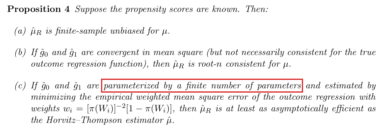
Proposition 3 (p. 7). Suppose the propensity scores are known. Then a finite-sample-valid confidence interval for is , where is the mean of the square inverse of the propensity scores.
Proof, Appendix A (p. 16). The Horvitz–Thompson estimator can be written , where . Because the outcome is binary, the bound holds with probability one. Recall that , so by Hoeffding’s inequality,
The problem
The proof conditions on the covariate vector and applies Hoeffding’s inequality to the deviation of from . Conditional on , however, the mean of need not equal . Let and . Then ; taking the expectation over gives the unconditional identity that the proof recalls. Hoeffding’s inequality bounds the conditional probability that exceeds the printed radius. It does not bound , and the printed radius does not account for the variation of around .
The proposition itself fails as stated. It claims coverage at least and states no restriction on . In the design that I give below, which satisfies every assumption of Section 2, the printed interval fails to contain with probability at . This level is far from the levels used in practice. The counterexample does not show that the printed interval undercovers at the 95% or 99% level: in the same design the probability that it fails to contain is below at both levels. These calculations do not settle whether the printed interval is valid at such levels in every design. To repair the proposition I keep the estimand, the estimator and the assumptions, and I widen the interval. A second Hoeffding bound controls , and I allot error probability to each of the two bounds. The corrected interval still has width of order .
Evidence an exact counterexample
The evidence is an exact counterexample to the printed statement and a derivation of the corrected one.
Counterexample. Let and . Let be uniform on , and set and . Let for and for , and assign the treatments independently given the covariates. The observations are i.i.d., the outcome and the treatment are binary, the covariate is continuous, consistency and unconfoundedness hold, positivity holds with , and . Let be the number of units such that , and let be the number of these units that are treated. In this design and , which implies that the printed interval depends on the sample only through . For , I have
The printed interval fails to contain exactly when . This inequality holds for 1946 of the 5151 pairs . Summing their probabilities in exact rational arithmetic, with rational bounds on the logarithm, I obtain
The conditional display in the proof fails more directly. On the event that for every , which has probability , the estimator equals and . On this event exceeds the printed radius, the left side of the display equals , and the right side equals .
The table lists, at three levels, the exact probability that each interval fails to contain in this design. Only the first entry of the first row exceeds its nominal level.
| Nominal level | Printed interval | Corrected interval |
|---|---|---|
Derivation of the corrected interval. Fix and set . By consistency, I have . Using unconfoundedness and the independence of the units, I find
and summing over , I obtain . Conditional on , the variables are independent and satisfy . Since , Hoeffding’s inequality implies that
for every that is a function of . Setting and taking the expectation over , I obtain
Next, the variables are i.i.d., take values in and have mean . Applying Hoeffding’s inequality to their mean, I have . If neither event occurs, then by the triangle inequality I have
By a union bound, I conclude that . Positivity implies that , and the width of the corrected interval is for fixed . For the alternative with a known bound such that with probability one, the variables are i.i.d., take values in and have mean , and Hoeffding’s inequality applied to their mean gives the radius .
What survives
The claim of the abstract and of p. 7 survives: with a binary outcome and a known propensity score, there exist finite-sample valid confidence intervals for whose width decreases at the rate . The corrected interval is one. The printed radius remains valid when the propensity score is constant, by unconditional Hoeffding’s inequality. Propositions 1, 2 and 4 and the numerical illustration of Section 3 do not use Proposition 3. What changes is the radius in Proposition 3, which becomes larger, the statement on p. 7 that the printed interval guarantees uniform validity, and the proof in Appendix A.
Corrected
Proposition 3. Suppose the propensity scores are known, and let . Under the assumptions of Section 2 (an i.i.d. sample, binary and , consistency, unconfoundedness and positivity), a finite-sample-valid confidence interval for is
where is the mean of the square inverse of the propensity scores. If a number is known such that with probability one, then is also a finite-sample-valid confidence interval for .
Proof, in place of the conditional display. Let be the outcome regression function. Recall that
so by Hoeffding’s inequality, with ,
The variables are i.i.d., take values in and have mean , so a second application of Hoeffding’s inequality gives . The triangle inequality and a union bound then give .


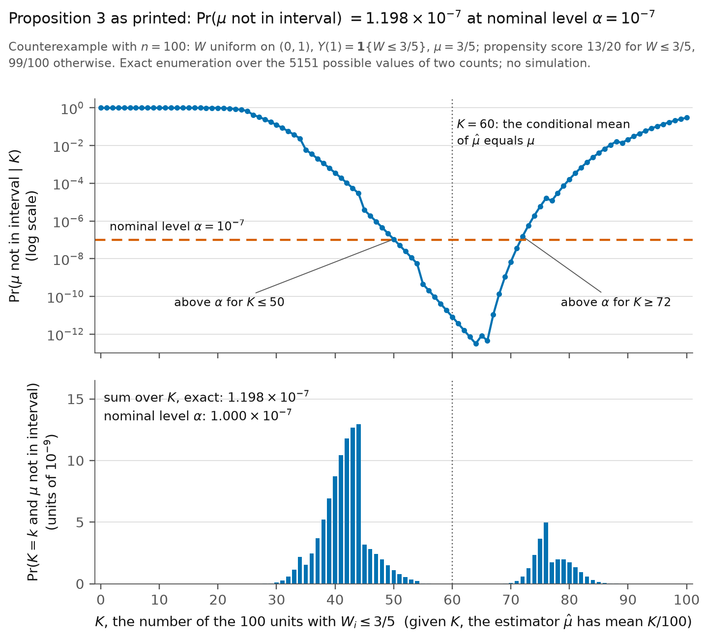
P046-E001 (, ), by the number of units such that . Top: the probability, given , that the printed interval fails to contain , on a logarithmic scale; the dashed line is the nominal level . Bottom: the contribution of each value of to that probability; the contributions sum to . Given , the estimator has mean , which equals only when .








My comment and the history of this entry