LLM-generated corrections to the published research of P. M. Aronow

Commentary/article P046

Corrections to: Nonparametric identification is not enough, but randomized controlled trials are

P. M. Aronow, James M. Robins, Theo Saarinen, Fredrik Sävje, and Jasjeet Sekhon (2025). Nonparametric identification is not enough, but randomized controlled trials are. Observational Studies 11(1):3–16.

DOI
10.1353/obs.2025.a956837
arXiv
2108.11342
Audited edition
Observational Studies, 2025, 11(1):3–16; 15 pages in the audited file
SHA-256 of the audited file
296af4ee19242f4cb3360da23d768c7af9c59e8c778ab1a832aa209ce6d317c3
Permanent address
https://pmaronow.github.io/llm-audit/works/P046/

Summary

The paper argues that randomized controlled trials are special among studies with unconfounded treatment. With a continuous confounder and an unknown propensity score, no uniformly consistent estimator of the average treatment effect exists without further assumptions. With a known propensity score, the paper presents unbiased, root-nn consistent estimators, which a simulation illustrates, and a finite-sample confidence interval. 3 entries are classified as errors (1 Moderate, 2 Minor), and 3 are clarity notes; one possible citation error remains unresolved. The Moderate error, P046-E001, is that the interval of Proposition 3 is not valid at every level. A wider interval is valid.

What was and was not checked

I checked the following points and found no error in them.

  • Proposition 1. The impossibility result for the model without further assumptions was rebuilt by two separate arguments for a lower bound, since the paper has no proof of it.
  • Proposition 2: the unbiasedness of the Horvitz–Thompson estimator, the variance bound 1/(nδ)1/(n\delta) with the uniform root-nn rate over populations with a common positivity constant δ>0\delta>0, and asymptotic normality for each fixed population.
  • The algebra of the exponent in the proof of Proposition 3. The centring of the bound is the subject of P046-E001.
  • The proof of Proposition 4(a), equality by equality, and parts (b) and (d) by a direct calculation of the conditional mean and variance of the summands, with part (d) read as in P046-E003. Part (c) is the subject of P046-E002.
  • The three data generating processes. Each has mean 1/21/2, the stated minima and maxima of the propensity score are approximately right, and Figure 2 and the code agree with the formulas.
  • The code against Section 3: the six estimators, the LOESS span and degree, the cross-fitting on opposite halves, the five sample sizes, and 10,000 replications in each of the 15 result files in the replication files. Two rules that the paper does not describe are the subject of P046-E005.
  • Figure 3 and Section 3.3. The figure was redrawn from the 15 result files and agrees with the published one within the precision of reading a graph, and the vertical shifts in the plotting script are the ones disclosed on p. 11. Two cells (n=1000n = 1000 under the second and third data generating processes) were recomputed with the authors' code and seed and agree with the stored bias and RMSE to about 10−1510^{-15}. A smaller new simulation (n=1000n = 1000 and n=10,000n = 10{,}000, with 2000 draws per cell) agrees with the stored RMSEs within Monte Carlo error. Every statement of Section 3.3 about orderings and rates agrees with the stored values.

The following limits apply to my checks.

  • The full simulation (five sample sizes, 10,000 draws per cell) was not repeated. The sample sizes 3162, 31,623 and 100,000 were compared from the result files only. Figure 3 prints no numbers, and its published values are readings from the graph.
  • Whether the interval of Proposition 3 as printed is valid at conventional levels in every design.
  • I checked three source pointers against publicly available passages and found nothing wrong: the original Robins–Wasserman post, search-indexed excerpts of Cao et al.'s author manuscript and the Chernozhukov preprint. The article of Robins and Ritov (1997) could not be obtained, and the attribution of Proposition 1 to its Theorem 3 was not checked. The version of record of Chernozhukov et al. was not read.
  • The bibliographic details of the reference list were not compared with the sources.

I do not infer that the rest of the paper is correct from an absence of corrections.

Headline claims and related corrections

  1. Under consistency, unconfoundedness and positivity with a continuous covariate, and without further assumptions, there is no uniformly consistent estimator of μ=E[Y(1)]\mu=\mathrm{E}[Y(1)], and hence no uniformly consistent estimator of the average treatment effect.

    Proposition 1 (attributed to Theorem 3 of Robins and Ritov 1997; no proof in the paper); abstract

    See P046-E004.

  2. When the propensity score is known, the Horvitz–Thompson estimator is unbiased, uniformly root-nn consistent and asymptotically normal for μ\mu, regardless of the complexity of the propensity-score function.

    Proposition 2; Figure 3

  3. With a binary outcome and a known propensity score, a finite-sample-valid confidence interval for μ\mu has width of order n−1/2n^{-1/2} regardless of the complexity of the score. The paper gives μ^±ξlog⁡(2/α)/(2n)\hat\mu\pm\sqrt{\xi\log(2/\alpha)/(2n)}, where ξ=n−1∑iπ(Wi)−2\xi=n^{-1}\sum_i\pi(W_i)^{-2}.

    Proposition 3 and its proof in Appendix A; abstract

    See P046-E001.

  4. With a known propensity score, the cross-fitted regression-adjusted estimator μ^R\hat\mu_R is finite-sample unbiased. If the fitted regressions converge in mean square, it is root-nn consistent even when their limits are misspecified. It is asymptotically at least as efficient as Horvitz–Thompson when a finite-parameter outcome model is fitted by weighted least squares with weights (1−π)/π2(1-\pi)/\pi^2, and semiparametrically efficient when the outcome regression is estimated consistently.

    Proposition 4(a)-(d); proof of 4(a) in Appendix A.

    See P046-E002, P046-E003.

  5. In the reported simulations, the RMSE of estimators that do not use the true propensity score does not decrease with nn under DGP 3, and the logistic-based estimators are inconsistent under DGP 2. HT and HTLOESS, which use the true score, converge at the parametric rate under all three designs.

    Figure 3; Section 3.3.

    See P046-E005.

  6. Regression adjustment with the true propensity score helps when the outcome regression can be learned (HTLOESS beats HT in DGP 1 and 2) and hurts when it cannot (HT beats HTLOESS in DGP 3), while the RMSE of HT is essentially the same in all three DGPs.

    Figure 3; Section 3.3

  7. Randomized controlled trials are special among studies with unconfounded treatment: a successfully executed trial has a statistical advantage beyond enforcing unconfoundedness, because it supplies the propensity score, so estimation and inference are fundamentally harder in observational settings.

    Propositions 1-4 and Figure 3; abstract; Section 4

    See P046-E001, P046-E002, P046-E004.

  8. Recording the assignment probabilities is enough to obtain the known-propensity benefits in natural or automated experiments; the analyst need not recover the complete assignment function.

    Propositions 2-4; Section 4 (Discussion).

    See P046-E001.

Corrections

Moderate (1)

A real substantive error with limited reach.

The interval of Proposition 3 is not finite-sample valid at every level, and its proof centres a conditional Hoeffding bound at μ\mu where the conditional mean of μ^\hat\mu is required; the interval with radius (ξ+1)log⁡(4/α)/(2n)(\sqrt{\xi}+1)\sqrt{\log(4/\alpha)/(2n)} is valid.

Proposition 3, p. 7 (PDF p. 6); its proof in Appendix A, pp. 15–16 (PDF pp. 14–15), at the display after “Recall that E[μ^]=μ\mathrm{E}[\hat\mu] = \mu, so by Hoeffding’s inequality,” on p. 16

See also under Formal statements (Lean): P046-T1, P046-T2, P046-T3, P046-T6

My comment on this entry

As printed

Proposition 3 (p. 7). Suppose the propensity scores are known. Then a finite-sample-valid 1−α1-\alpha confidence interval for μ\mu is μ^±ξlog⁡(2/α)/2n\hat\mu \pm \colorbox{#ffe58a}{$\sqrt{\xi \log(2/\alpha)/2n}$}, where ξ=n−1∑i=1n[π(Wi)]−2\xi = n^{-1}\sum_{i=1}^n [\pi(W_i)]^{-2} is the mean of the square inverse of the propensity scores.

Proof, Appendix A (p. 16). The Horvitz–Thompson estimator can be written μ^=∑i=1nAi\hat\mu = \sum_{i=1}^n A_i, where Ai=[nπ(Wi)]−1XiYiA_i = [n\pi(W_i)]^{-1}X_iY_i. Because the outcome is binary, the bound 0≤Ai≤[nπ(Wi)]−10 \le A_i \le [n\pi(W_i)]^{-1} holds with probability one. Recall that E[μ^]=μ\mathrm{E}[\hat\mu] = \mu, so by Hoeffding’s inequality,

Pr⁡(∣μ^−μ∣≥ξlog⁡(2/α)/2n∣W)≤2exp⁡(−2ξlog⁡(2/α)/2n∑i=1n[nπ(Wi)]−2).\Pr\Bigl( |\hat\mu - \colorbox{#ffe58a}{$\displaystyle \mu$}| \ge \sqrt{\xi \log(2/\alpha)/2n} \Bigm| \mathbf{W} \Bigr) \le 2\exp\biggl( \frac{-2\xi \log(2/\alpha)/2n}{\sum_{i=1}^n [n\pi(W_i)]^{-2}} \biggr).
The problem

The proof conditions on the covariate vector W=(W1,…,Wn)\mathbf{W} = (W_1, \dots, W_n) and applies Hoeffding’s inequality to the deviation of μ^\hat\mu from μ\mu. Conditional on W\mathbf{W}, however, the mean of μ^\hat\mu need not equal μ\mu. Let m(w)=E[Yi(1)∣Wi=w]m(w) = \mathrm{E}[Y_i(1) \mid W_i = w] and μW=n−1∑i=1nm(Wi)\mu_{\mathbf{W}} = n^{-1}\sum_{i=1}^n m(W_i). Then E[μ^∣W]=μW\mathrm{E}[\hat\mu \mid \mathbf{W}] = \mu_{\mathbf{W}}; taking the expectation over W\mathbf{W} gives the unconditional identity E[μ^]=μ\mathrm{E}[\hat\mu] = \mu that the proof recalls. Hoeffding’s inequality bounds the conditional probability that ∣μ^−μW∣|\hat\mu - \mu_{\mathbf{W}}| exceeds the printed radius. It does not bound ∣μ^−μ∣|\hat\mu - \mu|, and the printed radius does not account for the variation of μW\mu_{\mathbf{W}} around μ\mu.

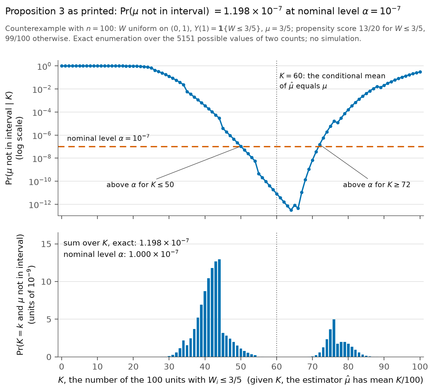
The proposition itself fails as stated. It claims coverage at least 1−α1-\alpha and states no restriction on α\alpha. In the design that I give below, which satisfies every assumption of Section 2, the printed interval fails to contain μ\mu with probability 1.198×10−71.198 \times 10^{-7} at α=10−7\alpha = 10^{-7}. This level is far from the levels used in practice. The counterexample does not show that the printed interval undercovers at the 95% or 99% level: in the same design the probability that it fails to contain μ\mu is below α\alpha at both levels. These calculations do not settle whether the printed interval is valid at such levels in every design. To repair the proposition I keep the estimand, the estimator and the assumptions, and I widen the interval. A second Hoeffding bound controls μW−μ\mu_{\mathbf{W}} - \mu, and I allot error probability α/2\alpha/2 to each of the two bounds. The corrected interval still has width of order n−1/2n^{-1/2}.

Evidence an exact counterexample

The evidence is an exact counterexample to the printed statement and a derivation of the corrected one.

Counterexample. Let n=100n = 100 and α=10−7\alpha = 10^{-7}. Let WiW_i be uniform on (0,1)(0,1), and set Yi(1)=1{Wi≤3/5}Y_i(1) = \mathbf{1}\{W_i \le 3/5\} and Yi(0)=0Y_i(0) = 0. Let π(w)=13/20\pi(w) = 13/20 for w≤3/5w \le 3/5 and π(w)=99/100\pi(w) = 99/100 for w>3/5w > 3/5, and assign the treatments independently given the covariates. The observations are i.i.d., the outcome and the treatment are binary, the covariate is continuous, consistency and unconfoundedness hold, positivity holds with δ=1/200\delta = 1/200, and μ=3/5\mu = 3/5. Let KK be the number of units such that Wi≤3/5W_i \le 3/5, and let SS be the number of these units that are treated. In this design μ^=S/65\hat\mu = S/65 and ξ=[400K/169+10000(100−K)/9801]/100\xi = [400K/169 + 10000(100-K)/9801]/100, which implies that the printed interval depends on the sample only through (K,S)(K, S). For 0≤s≤k≤1000 \le s \le k \le 100, I have

Pr⁡(K=k, S=s)=(100k)(ks)39s 21k−s 40100−k100100.\Pr(K = k,\, S = s) = \binom{100}{k}\binom{k}{s}\frac{39^s\, 21^{k-s}\, 40^{100-k}}{100^{100}}.

The printed interval fails to contain μ\mu exactly when 200(S/65−3/5)2/ξ>log⁡(2⋅107)200(S/65 - 3/5)^2/\xi > \log(2 \cdot 10^7). This inequality holds for 1946 of the 5151 pairs (k,s)(k,s). Summing their probabilities in exact rational arithmetic, with rational bounds on the logarithm, I obtain

Pr⁡(∣μ^−μ∣>ξlog⁡(2/α)/2n)=1.19792910697956…×10−7>10−7=α.\Pr\Bigl( |\hat\mu - \mu| > \sqrt{\xi \log(2/\alpha)/2n} \Bigr) = 1.19792910697956\ldots \times 10^{-7} > 10^{-7} = \alpha.

The conditional display in the proof fails more directly. On the event that Wi>3/5W_i > 3/5 for every ii, which has probability (2/5)100>0(2/5)^{100} > 0, the estimator μ^\hat\mu equals 00 and ξ=(100/99)2\xi = (100/99)^2. On this event ∣μ^−μ∣=3/5|\hat\mu - \mu| = 3/5 exceeds the printed radius, the left side of the display equals 11, and the right side equals 10−710^{-7}.

The table lists, at three levels, the exact probability that each interval fails to contain μ\mu in this design. Only the first entry of the first row exceeds its nominal level.

Exact probability that the interval fails to contain μ\mu in the counterexample (n=100n = 100), for the printed radius and for the corrected radius.
Nominal level α\alphaPrinted intervalCorrected interval
10−710^{-7}1.198×10⁻⁷\colorbox{#ffe58a}{$1.198 \times 10^{-7}$}1.207×10−231.207 \times 10^{-23}
0.050.050.013810.013812.324×10−62.324 \times 10^{-6}
0.010.010.0036140.0036142.396×10−82.396 \times 10^{-8}

Derivation of the corrected interval. Fix α∈(0,1)\alpha \in (0,1) and set c=log⁡(4/α)/(2n)c = \sqrt{\log(4/\alpha)/(2n)}. By consistency, I have XiYi=XiYi(1)X_iY_i = X_iY_i(1). Using unconfoundedness and the independence of the units, I find

E[Ai∣W]=E[Xi∣Wi] E[Yi(1)∣Wi]nπ(Wi)=m(Wi)n,\mathrm{E}[A_i \mid \mathbf{W}] = \frac{\mathrm{E}[X_i \mid W_i]\,\mathrm{E}[Y_i(1) \mid W_i]}{n\pi(W_i)} = \frac{m(W_i)}{n},

and summing over ii, I obtain E[μ^∣W]=μW\mathrm{E}[\hat\mu \mid \mathbf{W}] = \mu_{\mathbf{W}}. Conditional on W\mathbf{W}, the variables AiA_i are independent and satisfy 0≤Ai≤[nπ(Wi)]−10 \le A_i \le [n\pi(W_i)]^{-1}. Since ∑i=1n[nπ(Wi)]−2=ξ/n\sum_{i=1}^n [n\pi(W_i)]^{-2} = \xi/n, Hoeffding’s inequality implies that

Pr⁡(∣μ^−μW∣≥t∣W)≤2exp⁡(−2nt2/ξ)\Pr\bigl( |\hat\mu - \mu_{\mathbf{W}}| \ge t \bigm| \mathbf{W} \bigr) \le 2\exp(-2nt^2/\xi)

for every t>0t > 0 that is a function of W\mathbf{W}. Setting t=ξ ct = \sqrt{\xi}\,c and taking the expectation over W\mathbf{W}, I obtain

Pr⁡(∣μ^−μW∣≥ξ c)≤2exp⁡(−2nc2)=α/2.\Pr\bigl( |\hat\mu - \mu_{\mathbf{W}}| \ge \sqrt{\xi}\,c \bigr) \le 2\exp(-2nc^2) = \alpha/2.

Next, the variables m(Wi)m(W_i) are i.i.d., take values in [0,1][0,1] and have mean μ\mu. Applying Hoeffding’s inequality to their mean, I have Pr⁡(∣μW−μ∣≥c)≤2exp⁡(−2nc2)=α/2\Pr(|\mu_{\mathbf{W}} - \mu| \ge c) \le 2\exp(-2nc^2) = \alpha/2. If neither event occurs, then by the triangle inequality I have

∣μ^−μ∣≤∣μ^−μW∣+∣μW−μ∣<(ξ+1)c.|\hat\mu - \mu| \le |\hat\mu - \mu_{\mathbf{W}}| + |\mu_{\mathbf{W}} - \mu| < (\sqrt{\xi}+1)c.

By a union bound, I conclude that Pr⁡(∣μ^−μ∣≥(ξ+1)c)≤α\Pr(|\hat\mu - \mu| \ge (\sqrt{\xi}+1)c) \le \alpha. Positivity implies that ξ<δ−1\sqrt{\xi} < \delta^{-1}, and the width of the corrected interval is O(n−1/2)O(n^{-1/2}) for fixed α\alpha. For the alternative with a known bound b>0b > 0 such that π(Wi)≥b\pi(W_i) \ge b with probability one, the variables XiYi/π(Wi)X_iY_i/\pi(W_i) are i.i.d., take values in [0,b−1][0, b^{-1}] and have mean μ\mu, and Hoeffding’s inequality applied to their mean μ^\hat\mu gives the radius b−1log⁡(2/α)/(2n)b^{-1}\sqrt{\log(2/\alpha)/(2n)}.

What survives

The claim of the abstract and of p. 7 survives: with a binary outcome and a known propensity score, there exist finite-sample valid confidence intervals for μ\mu whose width decreases at the rate n−1/2n^{-1/2}. The corrected interval is one. The printed radius remains valid when the propensity score is constant, by unconditional Hoeffding’s inequality. Propositions 1, 2 and 4 and the numerical illustration of Section 3 do not use Proposition 3. What changes is the radius in Proposition 3, which becomes larger, the statement on p. 7 that the printed interval guarantees uniform validity, and the proof in Appendix A.

Corrected

Proposition 3. Suppose the propensity scores are known, and let 0<α<10 < \alpha < 1. Under the assumptions of Section 2 (an i.i.d. sample, binary YiY_i and XiX_i, consistency, unconfoundedness and positivity), a finite-sample-valid 1−α1-\alpha confidence interval for μ=E[Yi(1)]\mu = \mathrm{E}[Y_i(1)] is

μ^±(ξ+1)log⁡(4/α)/(2n),\hat\mu \pm \colorbox{#ffe58a}{$\displaystyle (\sqrt{\xi}+1)\sqrt{\log(4/\alpha)/(2n)}$},

where ξ=n−1∑i=1n[π(Wi)]−2\xi = n^{-1}\sum_{i=1}^n [\pi(W_i)]^{-2} is the mean of the square inverse of the propensity scores. If a number b>0b > 0 is known such that π(Wi)≥b\pi(W_i) \ge b with probability one, then μ^±b−1log⁡(2/α)/(2n)\hat\mu \pm b^{-1}\sqrt{\log(2/\alpha)/(2n)} is also a finite-sample-valid 1−α1-\alpha confidence interval for μ\mu.

Proof, in place of the conditional display. Let m(w)=E[Yi(1)∣Wi=w]m(w) = \mathrm{E}[Y_i(1) \mid W_i = w] be the outcome regression function. Recall that

E[μ^∣W]=μW,where μW=1n∑i=1nm(Wi),\colorbox{#ffe58a}{$\displaystyle \mathrm{E}[\hat\mu \mid \mathbf{W}] = \mu_{\mathbf{W}}$}, \qquad \text{where } \mu_{\mathbf{W}} = \frac{1}{n}\sum_{i=1}^n m(W_i),

so by Hoeffding’s inequality, with c=log⁡(4/α)/(2n)c = \sqrt{\log(4/\alpha)/(2n)},

Pr⁡(∣μ^−μW∣≥ξ c∣W)≤2exp⁡(−2ξc2∑i=1n[nπ(Wi)]−2)=α2.\Pr\Bigl( |\hat\mu - \colorbox{#ffe58a}{$\displaystyle \mu_{\mathbf{W}}$}| \ge \sqrt{\xi}\,c \Bigm| \mathbf{W} \Bigr) \le 2\exp\biggl( \frac{-2\xi c^2}{\sum_{i=1}^n [n\pi(W_i)]^{-2}} \biggr) = \frac{\alpha}{2}.

The variables m(Wi)m(W_i) are i.i.d., take values in [0,1][0,1] and have mean μ\mu, so a second application of Hoeffding’s inequality gives Pr⁡(∣μW−μ∣≥c)≤α/2\Pr(|\mu_{\mathbf{W}} - \mu| \ge c) \le \alpha/2. The triangle inequality and a union bound then give Pr⁡(∣μ^−μ∣≥(ξ+1)c)≤α\Pr(|\hat\mu - \mu| \ge (\sqrt{\xi}+1)c) \le \alpha.

Crop of five lines. The first two lines end the preceding paragraph: This confidence interval is finite-sample valid, meaning that its coverage is guaranteed to be greater or equal to its nominal level even in small samples. Proposition 3 follows: Suppose the propensity scores are known. Then a finite-sample-valid 1 minus alpha confidence interval for mu is mu-hat plus or minus the square root of xi log(2/alpha)/2n, where xi is the mean of the square inverse of the propensity scores. A red outline surrounds the square root of xi log(2/alpha)/2n.
Proposition 3, p. 7 (PDF p. 6), with the two lines that precede it. The outline marks the radius of the printed interval.
Crop of three lines of text and one displayed inequality. The text reads: The Horvitz-Thompson estimator can be written mu-hat equals the sum of the A-i, where A-i equals X-i Y-i divided by n pi(W-i). Because the outcome is binary, the bound 0 at most A-i at most 1 over n pi(W-i) holds with probability one. Recall that E[mu-hat] = mu, so by Hoeffding's inequality. The display states that the probability, conditional on W, that the absolute value of mu-hat minus mu is at least the square root of xi log(2/alpha)/2n is at most 2 exp of minus 2 xi log(2/alpha)/2n divided by the sum over i of n pi(W-i) to the power minus 2. Red outlines surround E[mu-hat] = mu in the text and the second mu inside the absolute value in the display.
Proof of Proposition 3, Appendix A, p. 16 (PDF p. 15). The outlines mark the unconditional identity E[μ^]=μ\mathrm{E}[\hat\mu] = \mu that the proof recalls and the centre μ\mu of the conditional bound.
Two panels that share a horizontal axis, K from 0 to 100, under the title: Proposition 3 as printed: the probability that mu is not in the interval equals 1.198 times 10 to the minus 7 at nominal level alpha equal to 10 to the minus 7. The top panel is a blue curve, on a logarithmic vertical axis, of the probability that mu is not in the interval given K. The curve equals 1 for K below about 17, falls to about 3 times 10 to the minus 13 near K equal to 64, and rises again to about 0.3 at K equal to 100. A dashed orange horizontal line marks the nominal level 10 to the minus 7; the curve is above this line for K at most 50 and for K at least 72. A dotted vertical line at K equal to 60 is labelled: the conditional mean of mu-hat equals mu. The bottom panel is a bar chart of the probability that K equals k and mu is not in the interval, in units of 10 to the minus 9. The bars form two groups, one between K equal to 29 and 54 with a maximum of about 12.9 at K equal to 44, and a smaller one between K equal to 70 and 86 with a maximum of about 5 at K equal to 76. A label gives the exact sum over K, 1.198 times 10 to the minus 7, above the nominal level, 1.000 times 10 to the minus 7.
The counterexample for P046-E001 (n=100n = 100, α=10−7\alpha = 10^{-7}), by the number KK of units such that Wi≤3/5W_i \le 3/5. Top: the probability, given KK, that the printed interval fails to contain μ\mu, on a logarithmic scale; the dashed line is the nominal level α\alpha. Bottom: the contribution of each value of KK to that probability; the contributions sum to 1.198×10−71.198 \times 10^{-7}. Given KK, the estimator μ^\hat\mu has mean K/100K/100, which equals μ=3/5\mu = 3/5 only when K=60K = 60.
My comment and the history of this entry

Agreed.

  1. Classification before my review (the classification when the audit was first completed, before I reviewed it): Moderate error.
  2. I commented.
  3. Independent evaluation. No change was needed: my comment agrees with the entry.

Minor (2)

Real but inconsequential, for example a misprint that does not change a result.

Seven sentences have errors of agreement or wording, and one reference repeats the label “doi:”.

Seven sentences on pp. 6, 7, 10, 11 and 12 (PDF pp. 5, 6, 9, 10 and 11), and the Aronow–Middleton entry of the reference list, p. 13 (PDF p. 12)

As printed
  1. p. 6. the strength of our statistical procedures critically depend on the assumptions brought to bear.
  2. p. 7. we consider a regression-based estimator of μ\mu that use a simple type of cross-fitting.
  3. p. 10. where g^0\hat g_0 and g^1\hat g_1 are cross-fitted LOESS regression of the same type as above.
  4. p. 11. only the two estimators that use of the true propensity score perform well.
  5. p. 11. and trying to do so introduce unnecessary noise
  6. p. 12. Knowledge of the propensity score can enormously beneficial in such settings.
  7. p. 12. because the input space tend to be high-dimensional
  8. p. 13. Peter M. Aronow and Joel A. Middleton. A class of unbiased estimators of the average treatment effect in randomized experiments. Journal of Causal Inference, 1(1):135–154, 2013. doi: doi:10.1515/jci-2012-0009. URL https://doi.org/10.1515/jci-2012-0009.
The problem

Items 1 to 7 are errors of grammar: a singular subject with a plural verb in items 1, 2, 5 and 7, a singular noun for the two fitted regressions in item 3, an extra “of” in item 4, and a missing “be” in item 6. The reference in item 8 prints the label “doi:” twice.

Evidence a check of the printed page

I checked the pages. On p. 7 the paper calls g^0\hat g_0 and g^1\hat g_1 “two estimators of the regression function”, which supports the plural in item 3.

What survives

The intended meaning is clear in every case, and no statement, formula or number changes.

Corrected
  1. the strength of our statistical procedures critically depends on the assumptions brought to bear.
  2. we consider a regression-based estimator of μ\mu that uses a simple type of cross-fitting.
  3. where g^0\hat g_0 and g^1\hat g_1 are cross-fitted LOESS regressions of the same type as above.
  4. only the two estimators that use the true propensity score perform well.
  5. and trying to do so introduces unnecessary noise
  6. Knowledge of the propensity score can be enormously beneficial in such settings.
  7. because the input space tends to be high-dimensional
  8. P. M. Aronow and Joel A. Middleton. A class of unbiased estimators of the average treatment effect in randomized experiments. Journal of Causal Inference, 1(1):135–154, 2013. doi: 10.1515/jci-2012-0009. URL https://doi.org/10.1515/jci-2012-0009.
Crop of three lines. The passage begins: trade-off: when the assignment mechanism is unknown, the strength of our statistical procedures critically depend on the assumptions brought to bear. A red outline surrounds the word depend.
Item 1: Section 2, p. 6 (PDF p. 5). The outline marks “depend”.
Crop of three lines. The passage includes: To ground these ideas, we consider a regression-based estimator of mu that use a simple type of cross-fitting. A red outline surrounds the word use.
Item 2: Section 2, p. 7 (PDF p. 6). The outline marks “use”.
Crop of three lines. The passage includes: in Proposition 4, where g-hat-0 and g-hat-1 are cross-fitted LOESS regression of the same type as above. A red outline surrounds the word regression.
Item 3: Section 3.2, p. 10 (PDF p. 9). The outline marks “regression”.
Crop of three lines. The sentence reads: For the third data generating process, which is the highly discontinuous function, only the two estimators that use of the true propensity score perform well. A red outline surrounds the words use of.
Item 4: Section 3.3, p. 11 (PDF p. 10). The outline marks “use of”.
Crop of three lines. The sentence reads: The explanation is that it is essentially impossible to capture the outcome regression function here, and trying to do so introduce unnecessary noise, which makes the precision worse. A red outline surrounds the word introduce.
Item 5: Section 3.3, p. 11 (PDF p. 10). The outline marks “introduce”.
Crop of three lines. The sentence reads: Knowledge of the propensity score can enormously beneficial in such settings. A red outline surrounds the words can enormously beneficial, at the start of the second line.
Item 6: Section 4, p. 12 (PDF p. 11). The outline marks “can enormously beneficial”.
Crop of three lines. The sentence reads: The estimation difficulties are often profound because the input space tend to be high-dimensional, and the treatment assignment function and the outcome regression tend to be highly non-smooth with discontinuities. A red outline surrounds the first word tend, at the start of the second line.
Item 7: Section 4, p. 12 (PDF p. 11). The outline marks “tend”.
Crop of the three lines of the reference by P. M. Aronow and Joel A. Middleton, A class of unbiased estimators of the average treatment effect in randomized experiments, Journal of Causal Inference, 2013. The third line reads: 2013. doi: doi:10.1515/jci-2012-0009, followed by the URL. A red outline surrounds the words doi: doi:.
Item 8: References, p. 13 (PDF p. 12). The outline marks the repeated label “doi: doi:”.

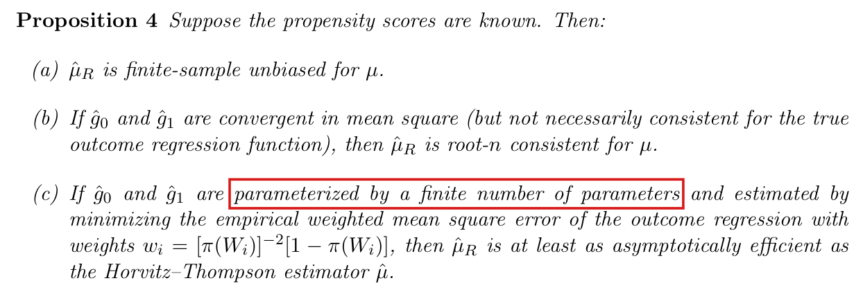
Proposition 4(c) holds when the working family of outcome regressions contains the zero function and the fitted regressions converge; for other families the adjusted estimator can be less efficient than the Horvitz–Thompson estimator.

Proposition 4(c), p. 8 (PDF p. 7)

See also under Formal statements (Lean): P046-T4, P046-T5

My comment on this entry

As printed

Proposition 4 Suppose the propensity scores are known. Then: …

(c) If g^0\hat g_0 and g^1\hat g_1 are parameterized by a finite number of parameters and estimated by minimizing the empirical weighted mean square error of the outcome regression with weights wi=[π(Wi)]−2[1−π(Wi)]w_i = [\pi(W_i)]^{-2}[1 - \pi(W_i)], then μ^R\hat\mu_R is at least as asymptotically efficient as the Horvitz–Thompson estimator μ^\hat\mu.

The problem

Note that the Horvitz–Thompson estimator is the adjusted estimator μ^R\hat\mu_R with the zero function in place of g^0\hat g_0 and g^1\hat g_1. For a fixed function gg, the summand of μ^R\hat\mu_R has variance Var⁡(Yi(1))+R(g)\operatorname{Var}(Y_i(1)) + R(g), where

R(g)=E[1−π(Wi)π(Wi)(Yi(1)−g(Wi))2],R(g) = \mathrm{E}\biggl[ \frac{1 - \pi(W_i)}{\pi(W_i)}\bigl( Y_i(1) - g(W_i) \bigr)^2 \biggr],

and the printed weights make the population weighted least-squares criterion on the treated units proportional to R(g)R(g). The fit minimizes RR only over the family of functions in which the two regressions are fitted, which I call the working family. The comparison with the Horvitz–Thompson estimator requires that the limit g∗g_* of the fit satisfy R(g∗)≤R(0)R(g_*) \le R(0). This holds when the working family contains the zero function, and it can fail otherwise. Part (c) as printed admits every family with a finite number of parameters. Every linear model with freely fitted coefficients contains the zero function, and the usual working models satisfy this condition.

Evidence an exact counterexample

The evidence is an exact counterexample to the printed statement and a derivation of the corrected one.

Counterexample. Let WiW_i be uniform on (0,1)(0,1), let Li=1{Wi≤1/2}L_i = \mathbf{1}\{W_i \le 1/2\}, and let ZiZ_i be a Bernoulli variable with mean 1/101/10 that is independent of WiW_i. Set Yi(0)=Yi(1)=LiZiY_i(0) = Y_i(1) = L_iZ_i. Let XiX_i be independent of ZiZ_i given WiW_i, with π(Wi)=1/4\pi(W_i) = 1/4 if Li=1L_i = 1 and π(Wi)=3/4\pi(W_i) = 3/4 if Li=0L_i = 0. The assumptions of Section 2 hold, with δ=1/8\delta = 1/8 in the positivity condition, and μ=1/20\mu = 1/20. Consider the working family of the functions gθ(w)=(1/2)1{w≤1/2}+θ 1{w>1/2}g_\theta(w) = (1/2)\mathbf{1}\{w \le 1/2\} + \theta\,\mathbf{1}\{w > 1/2\} with θ∈R\theta \in \mathbb{R}. It has one parameter and does not contain the zero function. The printed weights equal 1212 where Li=1L_i = 1 and 4/94/9 where Li=0L_i = 0. Since Yi=0Y_i = 0 where Li=0L_i = 0, the weighted criterion on any training fold equals a term that does not depend on θ\theta plus (4/9)Nθ2(4/9)N\theta^2, where NN is the number of treated units of the training fold such that Li=0L_i = 0. The value θ=0\theta = 0 minimizes it for every training fold (I take θ=0\theta = 0 when N=0N = 0), and θ=0\theta = 0 is the unique minimizer of the population criterion R(gθ)=3/8+θ2/6R(g_\theta) = 3/8 + \theta^2/6. With g∗(w)=(1/2)1{w≤1/2}g_*(w) = (1/2)\mathbf{1}\{w \le 1/2\}, I therefore have g^0=g^1=g∗\hat g_0 = \hat g_1 = g_*, and μ^R\hat\mu_R is the mean of the i.i.d. variables Ai=Xi[Yi−g∗(Wi)]/π(Wi)+g∗(Wi)A_i = X_i[Y_i - g_*(W_i)]/\pi(W_i) + g_*(W_i). The table lists the values of AiA_i and of the Horvitz–Thompson summand Hi=XiYi/π(Wi)H_i = X_iY_i/\pi(W_i).

The summands of the two estimators in the counterexample.
EventProbabilityAiA_iHiH_i
Li=1L_i = 1, Xi=0X_i = 03/83/81/21/200
Li=1L_i = 1, Xi=1X_i = 1, Zi=0Z_i = 09/809/80−3/2-3/200
Li=1L_i = 1, Xi=1X_i = 1, Zi=1Z_i = 11/801/805/25/244
Li=0L_i = 01/21/20000

A direct computation gives E[Ai]=E[Hi]=1/20\mathrm{E}[A_i] = \mathrm{E}[H_i] = 1/20, E[Ai2]=17/40\mathrm{E}[A_i^2] = 17/40 and E[Hi2]=1/5\mathrm{E}[H_i^2] = 1/5. For every nn, I obtain

Var⁡(μ^R)=169400n>79400n=Var⁡(μ^).\operatorname{Var}(\hat\mu_R) = \frac{169}{400n} > \frac{79}{400n} = \operatorname{Var}(\hat\mu).

In this example Var⁡(Yi(1))=19/400\operatorname{Var}(Y_i(1)) = 19/400, R(0)=3/20R(0) = 3/20 and R(g∗)=3/8R(g_*) = 3/8.

Derivation of the corrected statement. Fix a square-integrable function gg and write Ag=Yi(1)+(Xi/π(Wi)−1)(Yi(1)−g(Wi))A_g = Y_i(1) + (X_i/\pi(W_i) - 1)(Y_i(1) - g(W_i)) for the summand of μ^R\hat\mu_R. By unconfoundedness, conditional on (Wi,Yi(1))(W_i, Y_i(1)) the variable AgA_g has mean Yi(1)Y_i(1) and variance (1−π(Wi))π(Wi)−1(Yi(1)−g(Wi))2(1 - \pi(W_i))\pi(W_i)^{-1}(Y_i(1) - g(W_i))^2. By the law of total variance, I have Var⁡(Ag)=Var⁡(Yi(1))+R(g)\operatorname{Var}(A_g) = \operatorname{Var}(Y_i(1)) + R(g). For g=0g = 0 this is the variance of the Horvitz–Thompson summand. If the working family contains the zero function, then a minimizer g∗g_* of RR over the family satisfies R(g∗)≤R(0)R(g_*) \le R(0). Suppose that g^0\hat g_0 and g^1\hat g_1 converge to g∗g_* in L2L^2. Conditional on the training fold, the summands of the difference between μ^R\hat\mu_R and the mean of the variables Ag∗A_{g_*} have mean zero and second moment E[(1−π(Wi))π(Wi)−1(g^j(Wi)−g∗(Wi))2]\mathrm{E}[(1 - \pi(W_i))\pi(W_i)^{-1}(\hat g_j(W_i) - g_*(W_i))^2] over the evaluation fold, which implies that this difference is op(n−1/2)o_p(n^{-1/2}). Then n(μ^R−μ)\sqrt{n}(\hat\mu_R - \mu) has asymptotic variance Var⁡(Yi(1))+R(g∗)\operatorname{Var}(Y_i(1)) + R(g_*), which is at most the asymptotic variance Var⁡(Yi(1))+R(0)\operatorname{Var}(Y_i(1)) + R(0) of n(μ^−μ)\sqrt{n}(\hat\mu - \mu).

What survives

The sentence on p. 7 that adjustments “can be constructed so that they cannot harm, but can dramatically improve, asymptotic precision” asserts that suitable adjustments exist, and it stands. No other result of the paper relies on part (c), and the paper states on p. 10 that part (c) does not apply to its HTLOESS estimator. In the counterexample both estimators remain unbiased and root-nn consistent. What changes is the hypothesis of part (c).

Corrected

Proposition 4 Suppose the propensity scores are known. Then: …

(c) Suppose that g^0\hat g_0 and g^1\hat g_1 are estimated by minimizing the empirical weighted mean square error of the outcome regression with weights wi=[π(Wi)]−2[1−π(Wi)]w_i = [\pi(W_i)]^{-2}[1 - \pi(W_i)] over a fixed working family that is parameterized by a finite number of parameters and contains the zero function (or has the zero function in its weighted L2L^2 closure), and that both converge in L2L^2 to a deterministic minimizer over this family of

R(g)=E[1−π(Wi)π(Wi)(Yi(1)−g(Wi))2].\colorbox{#ffe58a}{$\displaystyle R(g) = \mathrm{E}\biggl[ \frac{1 - \pi(W_i)}{\pi(W_i)}\bigl( Y_i(1) - g(W_i) \bigr)^2 \biggr].$}

Then μ^R\hat\mu_R is at least as asymptotically efficient as the Horvitz–Thompson estimator μ^\hat\mu.

Crop of Proposition 4 from its first line through part (c). The first line reads: Proposition 4. Suppose the propensity scores are known. Then. Part (a): mu-hat-R is finite-sample unbiased for mu. Part (b): If g-hat-0 and g-hat-1 are convergent in mean square (but not necessarily consistent for the true outcome regression function), then mu-hat-R is root-n consistent for mu. Part (c): If g-hat-0 and g-hat-1 are parameterized by a finite number of parameters and estimated by minimizing the empirical weighted mean square error of the outcome regression with weights w-i equal to (1 minus pi(W-i)) divided by pi(W-i) squared, then mu-hat-R is at least as asymptotically efficient as the Horvitz-Thompson estimator mu-hat. A red outline surrounds the words parameterized by a finite number of parameters.
Proposition 4, parts (a) to (c), p. 8 (PDF p. 7). The outline marks the hypothesis of part (c) on the working family.
My comment and the history of this entry

Agreed.

  1. Classification before my review (the classification when the audit was first completed, before I reviewed it): Minor error.
  2. I commented.
  3. Independent evaluation. No change was needed: my comment agrees with the entry.

Clarity notes

Imprecise or ambiguous wording whose intended meaning is correct; not an error.

Assumptions on the outcome regression alone also permit a uniformly consistent estimator; the abstract names only assumptions on the propensity score function.

Abstract, third sentence, p. 3 (PDF p. 2)

See also under Formal statements (Lean): P046-T10

I disputed this classification, but as a rule, deferred to the models’ final judgment: see my comment and the history of this entry.

As printed

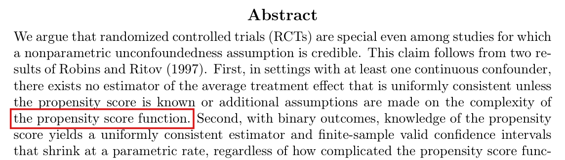
First, in settings with at least one continuous confounder, there exists no estimator of the average treatment effect that is uniformly consistent unless the propensity score is known or additional assumptions are made on the complexity of the propensity score function.

Intended meaning

The sentence summarizes Proposition 1, which states the impossibility “Without further assumptions”, and with this meaning it is correct. Read literally, the clause after “unless” lists every remedy, and the list is incomplete: suitable assumptions on the outcome regression alone also suffice, with the propensity score unknown and unrestricted. For example, suppose that E[Yi(x)∣Wi=w]=ax+h(w)\mathrm{E}[Y_i(x) \mid W_i = w] = a_x + h(w) for x∈{0,1}x \in \{0,1\}, where h(w)=min⁡{1,max⁡{0,w}}/4h(w) = \min\{1, \max\{0, w\}\}/4 is known and a0,a1∈[1/4,1/2]a_0, a_1 \in [1/4, 1/2] are unknown. Then the difference of the within-arm means of Yi−h(Wi)Y_i - h(W_i) (zero for an empty arm) estimates the average treatment effect with mean squared error at most (3/4)n+25/[2(n+1)](3/4)^n + 25/[2(n+1)], for every measurable propensity score such that 1/4<π(Wi)<3/41/4 < \pi(W_i) < 3/4. The body of the paper allows for such assumptions (the paragraph after Proposition 1 and footnote 1, p. 6), and no result depends on the literal reading.

Corrected

First, in settings with at least one continuous confounder, there exists no estimator of the average treatment effect that is uniformly consistent unless the propensity score is known or additional assumptions are made on the complexity of the outcome regression and/or propensity score functions.

Crop of the heading Abstract and the first eight lines of the abstract. The third sentence reads: First, in settings with at least one continuous confounder, there exists no estimator of the average treatment effect that is uniformly consistent unless the propensity score is known or additional assumptions are made on the complexity of the propensity score function. A red outline surrounds the words the propensity score function, at the start of the sixth line.
Abstract, p. 3 (PDF p. 2). The outline marks the phrase that names the propensity score function as the only object of the additional assumptions.

My comment and the history of this entry

Yes, this is what we meant but it was a misstatement.

Suggested classification: Minor error.

My position My comment above; I suggested a Minor error.

The models’ position Read with Proposition 1 and the remedies discussed in the body, the abstract's intended claim is correct. Assumptions on the outcome regression alone also permit a uniformly consistent estimator; the correction makes that omitted route explicit. Under the classification rule this is a clarity note.

  1. Classification before my review (the classification when the audit was first completed, before I reviewed it): clarity note.
  2. I commented and suggested a Minor error.
  3. Independent evaluation. Not adopted: my suggested rating (Minor) was not adopted; the claim is correct in context, so the entry stays a clarity note without an error severity.

“The semiparametric efficiency bound” in Proposition 4(d) is the bound of Hahn (1998) for an unrestricted covariate distribution, and with this meaning the statement holds whether or not the covariate distribution is known.

Proposition 4(d), p. 8 (PDF p. 7), with the set-up on p. 5 (PDF p. 4)

See also under Formal statements (Lean): P046-T9

As printed

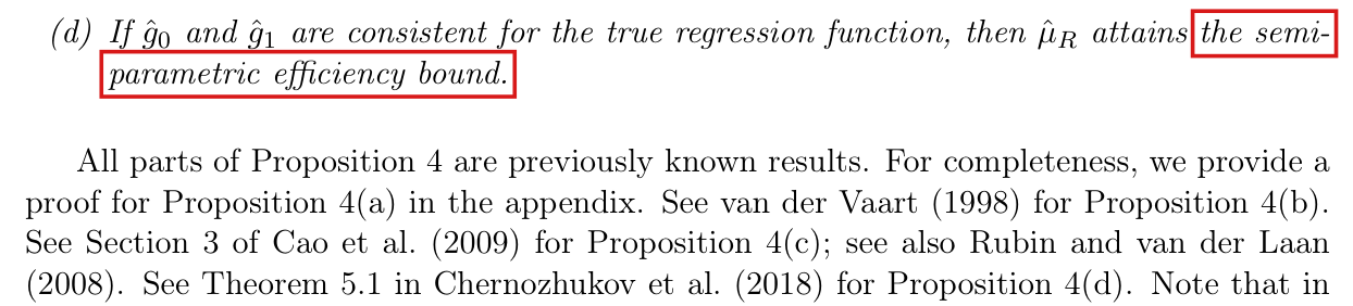
(d) If g^0\hat g_0 and g^1\hat g_1 are consistent for the true regression function, then μ^R\hat\mu_R attains the semiparametric efficiency bound.

Intended meaning

The paragraph after Proposition 4 cites Theorem 5.1 of Chernozhukov et al. (2018) for part (d). That theorem, as it appears in the preprint arXiv:1608.00060v6, names the efficiency bound of Hahn (1998), which is the bound in the model with an unrestricted distribution FWF_W of the covariate. Let m(w)=E[Yi(1)∣Wi=w]m(w) = \mathrm{E}[Y_i(1) \mid W_i = w]. For μ\mu and a known propensity score this bound equals E[m(Wi)(1−m(Wi))/π(Wi)]+Var⁡(m(Wi))\mathrm{E}[m(W_i)(1 - m(W_i))/\pi(W_i)] + \operatorname{Var}(m(W_i)), and μ^R\hat\mu_R attains it when g^0\hat g_0 and g^1\hat g_1 converge to mm in L2(FW)L^2(F_W), whether or not FWF_W is known. The set-up on p. 5 allows FWF_W to be “either known or unknown”. In the smaller model in which FWF_W is known the bound is lower by Var⁡(m(Wi))\operatorname{Var}(m(W_i)), and part (d) does not claim that μ^R\hat\mu_R attains that lower bound.

Corrected

(d) If ∥g^j−m∥L2(FW)→0\|\hat g_j - m\|_{L^2(F_W)} \to 0 in probability for j=0,1j = 0, 1, where m(w)=E[Yi(1)∣Wi=w]m(w) = \mathrm{E}[Y_i(1) \mid W_i = w], then μ^R\hat\mu_R attains the efficiency bound of Hahn (1998) for μ\mu in the model with a known propensity score and an unrestricted covariate distribution FWF_W, which equals E[m(Wi)(1−m(Wi))/π(Wi)]+Var⁡(m(Wi))\mathrm{E}[m(W_i)(1 - m(W_i))/\pi(W_i)] + \operatorname{Var}(m(W_i)).

Crop of part (d) of Proposition 4 and the first four lines of the next paragraph. Part (d) reads: If g-hat-0 and g-hat-1 are consistent for the true regression function, then mu-hat-R attains the semiparametric efficiency bound. Red outlines surround the words the semi-parametric efficiency bound, which run over a line break. The paragraph reads: All parts of Proposition 4 are previously known results. For completeness, we provide a proof for Proposition 4(a) in the appendix. See van der Vaart (1998) for Proposition 4(b). See Section 3 of Cao et al. (2009) for Proposition 4(c); see also Rubin and van der Laan (2008). See Theorem 5.1 in Chernozhukov et al. (2018) for Proposition 4(d).
Proposition 4(d) and the paragraph that follows the proposition, p. 8 (PDF p. 7). The outline marks “the semiparametric efficiency bound”; the last line shown cites Theorem 5.1 of Chernozhukov et al. (2018) for part (d).

The simulation code applies two rules that Section 3.2 does not state: a missing LOESS prediction is set to 0.50.5, and an estimated propensity score below 0.010.01 is set to 0.010.01.

Section 3.2, pp. 9–10 (PDF pp. 8–9)

As printed

p. 9. The second estimator, labelled LOESS, uses an LOESS regression for the predictions. We use LOESS regression with locally linear fits and the smoothing parameter, α\alpha, is set to 5N−1/35N^{-1/3}, where NN is the number of observations used in the regression.

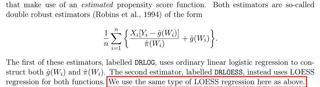
p. 10. The first of these estimators, labelled DRLOG, uses ordinary linear logistic regression to construct both g^(Wi)\hat g(W_i) and π^(Wi)\hat\pi(W_i). The second estimator, labelled DRLOESS, instead uses LOESS regression for both functions. We use the same type of LOESS regression here as above.

Intended meaning

The passages name the regression families, the degree and span of the LOESS fits and the estimator formulas, and nothing in them is false. They do not fully specify the estimators behind Figure 3. In the replication code (inesims.R), every LOESS prediction that is missing is replaced by 0.50.5, which enters LOESS, DRLOESS and HTLOESS, and the estimated propensity scores of DRLOG and DRLOESS are raised to 0.010.01 when they fall below it, with no upper cap. Both rules can take effect. Their effect on the reported RMSEs was not measured, and no reported value is shown to change.

Corrected

Add to Section 3.2: For every LOESS fit, missing predictions are replaced by 0.50.5. Estimated propensity scores used in DRLOG and DRLOESS are floored at 0.010.01 from below only, with no upper cap.

Crop of the last six lines of page 9. A red outline surrounds the sentence: The second estimator, labelled LOESS, uses an LOESS regression for the predictions. The text continues: We use LOESS regression with locally linear fits and the smoothing parameter, alpha, is set to 5 times N to the power minus one third, where N is the number of observations used in the regression. In this case, N is approximately n/2, because this is the number of observations with X-i equal to 1.
Section 3.2, p. 9 (PDF p. 8). The outline marks the sentence that introduces the LOESS estimator; the lines after it give the degree and span of the fits and no rule for missing predictions.
Crop of two lines of text, a displayed formula and three more lines. The text says that both estimators are so-called double robust estimators (Robins et al., 1994) of the form: one over n times the sum over i of X-i times (Y-i minus g-hat(W-i)) divided by pi-hat(W-i), plus g-hat(W-i). It continues: The first of these estimators, labelled DRLOG, uses ordinary linear logistic regression to construct both g-hat(W-i) and pi-hat(W-i). The second estimator, labelled DRLOESS, instead uses LOESS regression for both functions. We use the same type of LOESS regression here as above. A red outline surrounds the last sentence.
Section 3.2, p. 10 (PDF p. 9). The outline marks the last sentence of the description of the two estimators that use an estimated propensity score; the description states no lower limit for the estimated scores.

Formal statements (Lean)

Formal results: 9 whole; 0 restricted; 1 refuted; 0 omitted.

Coverage concerns the identified claim under its stated assumptions. A checked proof establishes the formal statement; correspondence to the published text was reviewed by AI. Repository access is currently required to open the source links.

Each result links to its current formal statement and proof. “Whole” covers the identified claim under its assumptions; “restricted” covers the stated narrower scope; “refuted” gives a counterexample to the identified assertion; “omitted” has no current theorem. Any named published theorem used as a premise remains an assumption. Browse the formal results for this work.

Proposition 3, as printed (the confidence interval)

p. 7 (PDF p. 6); restated in Appendix A, p. 15 (PDF p. 14)

Proposition 3, p. 7 (PDF p. 6), Appendix A, p. 15 (PDF p. 14). The specified continuous counterexample satisfies all standing assumptions. Its three category probabilities and joint count law, exact sample-statistic reductions, equivalent strict exclusion tests, 5151 feasible states and 1946 failures give the exact recorded noncoverage probability, exceeding 119/10^9 and alpha=10^(-7). The closed interval undercovers and the non-strict population tail also exceeds alpha. The decimal probability is specified by its exact rational value. Usual measure-theoretic conditions are assumed.

Historical component credits
  • Proved AronowAudit.P046.Wave1.counterexample_proof Historical support retained; baseline fidelity: ok; manifest: used; used in Solution; This is an exact witness to failure of the printed assertion, not a positive proof of Proposition 3. The rational certifiedCut selects exactly the logarithmic failure set; independent integer enumeration found 1946 states and the target mass. ValidStudy asserts, rather than assumes, the standing conditions here; strict noncoverage>alpha also implies the appendix weak-tail failure. The public description is accurate and does not claim failure at conventional confidence levels.
  • Proved AronowAudit.P046.IntervalExample.score_positivity Historical support retained; baseline fidelity: ok; manifest: used; used in Solution; The selected aggregate conclusion is used directly; this supporting declaration is not separately invoked.
  • Proved AronowAudit.P046.IntervalExample.log_lt_seventeen Historical support retained; baseline fidelity: ok; manifest: not used; not used in Solution; The exact 1946-state mass is retained; the separate threshold-17 lower-bound route is not used.
  • Proved AronowAudit.P046.IntervalExample.lower_mass_exceeds_alpha Historical support retained; baseline fidelity: ok; manifest: not used; not used in Solution; The exact 1946-state mass is retained; the separate threshold-17 lower-bound route is not used.
  • Proved AronowAudit.P046.Wave1.count_mass_bridge_proof Historical support retained; baseline fidelity: ok; manifest: not used; not used in Solution; The exact 1946-state mass is retained; the separate threshold-17 lower-bound route is not used.
  • Proved AronowAudit.P046.IntervalExample.cutoff_implies_squared_exclusion Historical support retained; baseline fidelity: ok; manifest: not used; not used in Solution; The exact 1946-state mass is retained; the separate threshold-17 lower-bound route is not used.
  • Proved AronowAudit.P046.IntervalExample.cutoff_state_count Historical support retained; baseline fidelity: ok; manifest: not used; not used in Solution; The exact 1946-state mass is retained; the separate threshold-17 lower-bound route is not used.
  • Proved AronowAudit.P046.unitUniform_Iic Historical support retained; baseline fidelity: ok; manifest: used; used in Solution; The selected aggregate conclusion is used directly; this supporting declaration is not separately invoked.
  • Proved AronowAudit.P046.unitUniform_singleton Historical support retained; baseline fidelity: ok; manifest: used; used in Solution; The selected aggregate conclusion is used directly; this supporting declaration is not separately invoked.
  • Proved AronowAudit.P046.unitUniform_bernE Historical support retained; baseline fidelity: ok; manifest: used; used in Solution; The selected aggregate conclusion is used directly; this supporting declaration is not separately invoked.
  • Proved AronowAudit.P046.IntervalExample.log_certified_bounds Historical support retained; baseline fidelity: ok; manifest: used; used in Solution; The selected aggregate conclusion is used directly; this supporting declaration is not separately invoked.
  • Proved AronowAudit.P046.IntervalExample.certified_state_count Historical support retained; baseline fidelity: ok; manifest: used; used in Solution; The selected aggregate conclusion is used directly; this supporting declaration is not separately invoked.
  • Proved AronowAudit.P046.IntervalExample.certified_partition Historical support retained; baseline fidelity: ok; manifest: used; used in Solution; The selected aggregate conclusion is used directly; this supporting declaration is not separately invoked.
  • Proved AronowAudit.P046.IntervalExample.certified_mass_exact Historical support retained; baseline fidelity: ok; manifest: used; used in Solution; Auxiliary exact integer certificate. It does not identify a sampling probability; that bridge is assigned to other declarations. Claim-stage verdict unchanged after reading the record.
  • Proved AronowAudit.P046.IntervalExample.certified_mass_gt Historical support retained; baseline fidelity: ok; manifest: used; used in Solution; The selected aggregate conclusion is used directly; this supporting declaration is not separately invoked.
  • Proved AronowAudit.P046.IntervalExample.count_deviation_sq Historical support retained; baseline fidelity: ok; manifest: used; used in Solution; The selected aggregate conclusion is used directly; this supporting declaration is not separately invoked.
  • Proved AronowAudit.P046.IntervalExample.certified_cut_iff_exclusion Historical support retained; baseline fidelity: ok; manifest: used; used in Solution; The selected aggregate conclusion is used directly; this supporting declaration is not separately invoked.
  • Proved AronowAudit.P046.IntervalExample.exact_failure_state_count Historical support retained; baseline fidelity: ok; manifest: used; used in Solution; The selected aggregate conclusion is used directly; this supporting declaration is not separately invoked.
  • Proved AronowAudit.P046.Wave1.exact_noncoverage_proof Historical support retained; baseline fidelity: ok; manifest: not used; not used in Solution; The selected aggregate conclusion is used directly; this supporting declaration is not separately invoked.
  • Proved AronowAudit.P046.unitUniform_probability Historical support retained; baseline fidelity: ok; manifest: used; used in Solution; The selected aggregate conclusion is used directly; this supporting declaration is not separately invoked.
  • Proved AronowAudit.P046.unitUniform_Ici Historical support retained; baseline fidelity: ok; manifest: not used; not used in Solution; The selected aggregate conclusion is used directly; this supporting declaration is not separately invoked.
  • Proved AronowAudit.P046.measurable_threshold Historical support retained; baseline fidelity: ok; manifest: used; used in Solution; The selected aggregate conclusion is used directly; this supporting declaration is not separately invoked.
  • Proved AronowAudit.P046.atomless_of_uniform_marginal Historical support retained; baseline fidelity: ok; manifest: used; used in Solution; The selected aggregate conclusion is used directly; this supporting declaration is not separately invoked.
  • Proved AronowAudit.P046.IntervalExample.measurable_generate Historical support retained; baseline fidelity: ok; manifest: used; used in Solution; The selected aggregate conclusion is used directly; this supporting declaration is not separately invoked.
  • Proved AronowAudit.P046.IntervalExample.covariate_law Historical support retained; baseline fidelity: ok; manifest: used; used in Solution; Equality with the uniform marginal is exact. Restricting volume to [0,1] rather than (0,1) changes no measure because the endpoints have zero Lebesgue mass. Claim-stage verdict unchanged after reading the record.
  • Proved AronowAudit.P046.IntervalExample.probability_continuity_mean Historical support retained; baseline fidelity: ok; manifest: used; used in Solution; The selected aggregate conclusion is used directly; this supporting declaration is not separately invoked.
  • Proved AronowAudit.P046.unitUniform_Iio Historical support retained; baseline fidelity: ok; manifest: not used; not used in Solution; The selected aggregate conclusion is used directly; this supporting declaration is not separately invoked.

Appendix A, proof of Proposition 3, the conditional Hoeffding display, as printed

p. 16 (PDF p. 15)

Appendix A, proof of Proposition 3, p. 16 (PDF p. 15). The specified valid continuous design has mu=1/2 and a covariate event of probability 2^(-100). For every covariate vector in this event and every treatment vector, the design outcomes, HT and the conditional centre mu_W vanish, and the absolute population error is 1/2. Almost everywhere on the event the actual conditional mean is zero, distinct from mu; the conditional tail is one while the full printed right side is 1/20. Usual measure-theoretic conditions are assumed; conditional expectations are asserted only up to almost-everywhere equality.

Historical component credits

Proposition 3, corrected (with the corrected proof)

p. 7 (PDF p. 6); proof in Appendix A, pp. 15-16 (PDF pp. 14-15)

corrected Proposition 3, p. 7 (PDF p. 6), proof pp. 15–16 (PDF pp. 14–15). The two-error and known-bound intervals have population coverage at least nominal. All corrected proof steps are included: conditional factorization and means, conditional independence and ranges, fixed and covariate-measurable random threshold bounds, i.i.d. regression sampling, triangle inclusion and union bound, strict positivity radius bound and inverse-square-root width rate, and the alternative's i.i.d. summands and Hoeffding calculation. Usual measure-theoretic conditions are assumed.

Historical component credits
  • Proved AronowAudit.P046.Wave1.proposition3_corrected_proof Historical support retained; baseline fidelity: ok; manifest: used; used in Solution; The comparison is to the corrected target T3, so widening the erroneous printed radius is not a mismatch with this credited claim.
  • Proved AronowAudit.P046.Wave1.ht_conditional_centre_proof Historical support retained; baseline fidelity: ok; manifest: used; used in Solution; This supports a corrected-proof step omitted from the restricted coverage-and-width statement; it is not separately invoked.
  • Proved AronowAudit.P046.Wave1.conditional_hoeffding_proof Historical support retained; baseline fidelity: ok; manifest: used; used in Solution; This supports a corrected-proof step omitted from the restricted coverage-and-width statement; it is not separately invoked.
  • Proved AronowAudit.P046.covariate_hoeffding Historical support retained; baseline fidelity: ok; manifest: used; used in Solution; This supports a corrected-proof step omitted from the restricted coverage-and-width statement; it is not separately invoked.
  • Proved AronowAudit.P046.proposition3_known_bound Historical support retained; baseline fidelity: ok; manifest: used; used in Solution; Fidelity sweep: ok
  • Proved AronowAudit.P046.two_error_union_bound Historical support retained; baseline fidelity: ok; manifest: used; used in Solution; This supports a corrected-proof step omitted from the restricted coverage-and-width statement; it is not separately invoked.
  • Proved AronowAudit.P046.sqrt_mean_inverse_sq_lt Historical support retained; baseline fidelity: ok; manifest: used; used in Solution; This supports a corrected-proof step omitted from the restricted coverage-and-width statement; it is not separately invoked.
  • Proved AronowAudit.P046.corrected_width Historical support retained; baseline fidelity: ok; manifest: used; used in Solution; Fidelity sweep: ok
  • Proved AronowAudit.P046.regression_mean Historical support retained; baseline fidelity: ok; manifest: used; used in Solution; This supports a corrected-proof step omitted from the restricted coverage-and-width statement; it is not separately invoked.
  • Proved AronowAudit.P046.muW_unbiased Historical support retained; baseline fidelity: ok; manifest: used; used in Solution; This supports a corrected-proof step omitted from the restricted coverage-and-width statement; it is not separately invoked.
  • Proved AronowAudit.P046.iid_mean_hoeffding Historical support retained; baseline fidelity: ok; manifest: used; used in Solution; This supports a corrected-proof step omitted from the restricted coverage-and-width statement; it is not separately invoked.

Proposition 4(c), as printed

p. 8 (PDF p. 7)

Proposition 4(c), p. 8 (PDF p. 7), treated-case weighted-loss reading. The specified continuous counterexample has exact balanced fits g_0, with all training loss decompositions and minimizer characterizations, the unique population minimizer, the scalar summand table, event probabilities and moments, and bounded i.i.d. summands. Both finite-sample variances and Gaussian limits reverse the printed efficiency ordering. Zero is outside the family and its weighted L2 closure; the potential-outcome variance and positive risk gap are explicit. Usual measure-theoretic conditions are assumed; sample sizes in estimator formulas are positive.

Historical component credits

Proposition 4(c), corrected

p. 8 (PDF p. 7)

corrected Proposition 4(c), p. 8 (PDF p. 7). The zero-benchmark square-integrable working-family theorem and the family-free direct risk-comparison theorem give both Gaussian limits and the efficiency ordering. The genuine extended L2 errors converge in probability; individual fitted functions may have infinite error on events whose probabilities vanish. Finite limit risk implies square integrability. The fixed-summand variance identity and equivalence of weighted and ordinary L2 norms are included. Usual measure-theoretic conditions are assumed; functions are measurable and Gaussian variance zero denotes a point mass.

Historical component credits
  • Proved AronowAudit.P046.Wave1.proposition4c_corrected_proof Historical support retained; baseline fidelity: ok; manifest: used; used in Solution; This is the corrected claim, not a proof of the false printed Proposition 4(c). hfitsL2 follows from hG and the membership part of hfit, as R267-10 states. Norm-squared convergence, sequential weighted closure, a.e. versions, and a degenerate Gaussian when V=0 change no cases.
  • Proved AronowAudit.P046.Wave1.proposition4c_direct_proof Limited support; baseline fidelity: narrower; manifest: used; used in Solution; {'source': 'adjudication+second review', 'adjudicator': "GP046B3b.lean:238 adds almost-sure MemLp membership at exponent 2 for every sample size and fold to T5's direct sufficient-condition component. That clause requires probabilistic L2-error convergence to a deterministic limit and R(gstar) <= R(0); it does not require the fitted functions to belong to the square-integrable working family in the separate empirical-minimization formulation. For uniform W, gstar=0, and a cross-fit equal to w^(-1/2) on an opposite-training-fold event of probability 1/n and zero otherwise, the genuine squared L2 error is infinite on that event and zero elsewhere, so it converges to zero in probability although hfitsL2 fails for every n >= 2. These fits have the same HT normal limit because the estimator differs from HT only on events of probability at most 2/n, so the excluded cases are not failures of the target conclusion.", 'suggested_fix': "Express hconv using the genuine extended L2 error, for example eLpNorm or the nonnegative lintegral of squared error, and remove hfitsL2 from the direct theorem. Localize the remainder argument to training events on which that error is small. Merely deleting hfitsL2 while retaining P046_Audit.lean:170's real-valued l2Sq is insufficient: Mathlib's Bochner integral assigns zero to nonintegrable squared errors (MeasureTheory/Integral/Bochner/Basic.lean:204).", 'second_review': "P046/Wave1/Gap/GP046B3b.lean:238 requires almost-sure MemLp membership for every sample size and fold, whereas T5's direct clause requires only L2-error convergence in probability and R(gstar) <= R(0). With uniform W on (0,1), independent fair binary treatment and potential outcomes, and gstar=0, opposite-training-fold fits 1_E*w^(-1/2) on events of probability 1/n satisfy the genuine extended-error convergence and retain the HT normal limit, but fail this membership hypothesis. The repair must both remove hfitsL2 and use an extended L2 error: l2Sq at P046/P046_Audit.lean:170 is a real Bochner integral, which assigns zero to nonintegrable squared errors by Mathlib/MeasureTheory/Integral/Bochner/Basic.lean:204.", 'severity': 'major'}
  • Proved AronowAudit.P046.Wave1.fixed_adjusted_variance_proof Historical support retained; baseline fidelity: ok; manifest: used; used in Solution; Auxiliary finite variance identities only; no empirical-minimizer consistency is asserted. The stated L2 hypothesis belongs to the target working-family setting, and no global Borel restriction on g is added.
  • Proved AronowAudit.P046.Wave1.population_weighted_criterion_proof Historical support retained; baseline fidelity: ok; manifest: used; used in Solution; The selected aggregate conclusion is used directly; this supporting declaration is not separately invoked.
  • Proved AronowAudit.P046.Wave1.zero_benchmark_risk_proof Historical support retained; baseline fidelity: ok; manifest: used; used in Solution; The selected aggregate conclusion is used directly; this supporting declaration is not separately invoked.
  • Proved AronowAudit.P046.adjusted_decomposition Historical support retained; baseline fidelity: ok; manifest: not used; not used in Solution; The selected aggregate conclusion is used directly; this supporting declaration is not separately invoked.
  • Proved AronowAudit.P046.bern_adjusted_mean Historical support retained; baseline fidelity: ok; manifest: not used; not used in Solution; The selected aggregate conclusion is used directly; this supporting declaration is not separately invoked.
  • Proved AronowAudit.P046.bern_adjusted_variance Historical support retained; baseline fidelity: ok; manifest: not used; not used in Solution; The selected aggregate conclusion is used directly; this supporting declaration is not separately invoked.
  • Proved AronowAudit.P046.risk_minimizer_zero Limited support; baseline fidelity: narrower; manifest: not used; not used in Solution; Requires actual zero membership; the selected corrected theorem also covers the canonical zero-closure alternative.
  • Proved AronowAudit.P046.Wave1.risk_expansion_cauchy_proof Historical support retained; baseline fidelity: ok; manifest: not used; not used in Solution; The selected aggregate conclusion is used directly; this supporting declaration is not separately invoked.
  • Proved AronowAudit.P046.fitted_L2_from_membership Historical support retained; baseline fidelity: ok; manifest: used; used in Solution; This is an equality-substitution auxiliary lemma, not evidence of minimizer existence or convergence. No validity hypothesis is needed for transport of MemLp along equality.

Proposition 3

p. 7 (PDF p. 6); proof in Appendix A, pp. 15-16 (PDF pp. 14-15)

The printed claim is false: P046-T6; Proposition 3, p. 7 (PDF p. 6), Appendix A, pp. 15–16 (PDF pp. 14–15). The universally quantified population-centred tail bound with the printed random radius fails for a valid study.

Historical component credits
  • Counterexample proved AronowAudit.P046.Wave1.proposition3_printed_refuted Historical support retained; baseline fidelity: ok; manifest: used; used in Solution; The target explicitly prints the weak tail event in the appendix, exactly as formalized. Even if the headline closed interval is read with strict failure, universal validity over all alpha in (0,1) is equivalent: a weak-tail violation of mass p>alpha yields strict undercoverage at any slightly larger alpha-prime<p, because the radius strictly decreases with alpha almost surely under positivity. No conventional-level or corrected-interval assertion is made.

Proposition 2

p. 6 (PDF p. 5); supporting sentence on p. 7 (PDF p. 6)

Proposition 2, p. 6 (PDF p. 5), supporting text p. 7 (PDF p. 6). HT is integrable and unbiased, uniformly root-n consistent for each common positive positivity constant, and asymptotically normal with the stated summand variance, including the variance-zero convention.

Historical component credits
  • Proved AronowAudit.P046.proposition2_asymptotic Historical support retained; baseline fidelity: ok; manifest: used; used in Solution; {'source': 'adjudication', 'decision': 'rejected', 'what': 'AronowAudit/P046/P046_Audit.lean:2177 combines common-delta uniform root-n consistency with a fixed-law NormalLimit having variance E[m(W)/pi(W)]-mu^2, exactly the two asymptotic components specified by target T7. The common-delta convention is explicit in the target’s definitions_needed, and unbiasedness is outside this asymptotic row’s stated component. NormalLimit at line 197 allows a point mass at zero variance, as the target expressly does. Binary outcomes and positivity make the displayed variance finite and nonnegative, so conversion to a nonnegative Gaussian variance discards no cases.'}
  • Proved AronowAudit.P046.ht_unbiased Historical support retained; baseline fidelity: ok; manifest: used; used in Solution; No substantive mismatch, circular premise, or totalization issue found; the verdict is unchanged from the independent claim stage.
  • Proved AronowAudit.P046.ht_second_moment Historical support retained; baseline fidelity: ok; manifest: used; used in Solution; No substantive mismatch, circular premise, or totalization issue found; the verdict is unchanged from the independent claim stage.
  • Proved AronowAudit.P046.ht_variance Historical support retained; baseline fidelity: ok; manifest: used; used in Solution; The selected aggregate conclusion is used directly; this supporting declaration is not separately invoked.
  • Proved AronowAudit.P046.ht_chebyshev Historical support retained; baseline fidelity: ok; manifest: used; used in Solution; The selected aggregate conclusion is used directly; this supporting declaration is not separately invoked.
  • Proved AronowAudit.P046.consistency_treated Historical support retained; baseline fidelity: ok; manifest: used; used in Solution; The selected aggregate conclusion is used directly; this supporting declaration is not separately invoked.
  • Proved AronowAudit.P046.ht_binary_range Historical support retained; baseline fidelity: ok; manifest: used; used in Solution; The selected aggregate conclusion is used directly; this supporting declaration is not separately invoked.
  • Proved AronowAudit.P046.bern_normalization Historical support retained; baseline fidelity: ok; manifest: not used; not used in Solution; The selected aggregate conclusion is used directly; this supporting declaration is not separately invoked.
  • Proved AronowAudit.P046.bern_ht_mean Historical support retained; baseline fidelity: ok; manifest: not used; not used in Solution; The selected aggregate conclusion is used directly; this supporting declaration is not separately invoked.
  • Proved AronowAudit.P046.bern_ht_second Historical support retained; baseline fidelity: ok; manifest: not used; not used in Solution; The selected aggregate conclusion is used directly; this supporting declaration is not separately invoked.
  • Proved AronowAudit.P046.iid_mean_variance Historical support retained; baseline fidelity: ok; manifest: used; used in Solution; The selected aggregate conclusion is used directly; this supporting declaration is not separately invoked.
  • Proved AronowAudit.P046.iid_mean_integral Historical support retained; baseline fidelity: ok; manifest: used; used in Solution; The selected aggregate conclusion is used directly; this supporting declaration is not separately invoked.
  • Proved AronowAudit.P046.conditional_xy_factorization Historical support retained; baseline fidelity: ok; manifest: used; used in Solution; The selected aggregate conclusion is used directly; this supporting declaration is not separately invoked.
  • Proved AronowAudit.P046.ht_unit_facts Historical support retained; baseline fidelity: ok; manifest: used; used in Solution; No substantive mismatch, circular premise, or totalization issue found; the verdict is unchanged from the independent claim stage.
  • Proved AronowAudit.P046.ht_unit_memLp Historical support retained; baseline fidelity: ok; manifest: used; used in Solution; The L2 property is the conclusion, derived from binary outcomes and the positive lower bound; it is not an added moment hypothesis.
  • Proved AronowAudit.P046.ht_sample_memLp Historical support retained; baseline fidelity: ok; manifest: used; used in Solution; n=0 is an innocuous extension: the empty sum divided by zero is zero; the supporting conclusion for every positive n is unchanged.
  • Proved AronowAudit.P046.ht_uniform_root_n Historical support retained; baseline fidelity: ok; manifest: used; used in Solution; {'source': 'adjudication', 'decision': 'rejected', 'what': 'AronowAudit/P046/P046_Audit.lean:2103 proves UniformRootN delta, whose definition at line 218 chooses the cutoff before the valid study and positive sample size. The target’s own definitions_needed explicitly defines uniform root-n consistency over the common-delta class P_delta, so this quantifier order matches the supplied claim interpretation rather than imposing a restriction found only in the row description. Although the paper leaves the uniformity class unspecified, that ambiguity is acknowledged in the target. Empty classes for delta≥1/2 do not make the result vacuous: a fair constant propensity gives nonempty valid classes for every 0<delta<1/2.'}
  • Proved AronowAudit.P046.iid_mean_normal Historical support retained; baseline fidelity: ok; manifest: used; used in Solution; The selected aggregate conclusion is used directly; this supporting declaration is not separately invoked.

Proposition 4(a)

p. 8 (PDF p. 7); proof in Appendix A, p. 16 (PDF p. 15)

Proposition 4(a), p. 8 (PDF p. 7), Appendix A, p. 16 (PDF p. 15). The cross-fitted regression estimator is finite-sample unbiased whenever its expectation exists, including cancellation between nonintegrable predictions. The consistency identity, three-term expansion, HT expectation chain, opposite-fold conditional independence, and fitted-term expectation and cancellation chains are included. Component expectation chains are asserted when their individual expectations exist. The usual measure-theoretic conditions are assumed. Arbitrary deterministic folds include roughly equal folds.

Historical component credits
  • Proved AronowAudit.P046.Wave1.proposition4a_proof Limited support; baseline fidelity: narrower; manifest: used; used in Solution; {'source': 'adjudication+second review', 'adjudicator': "GP046B4.lean:221 requires every evaluated cross-fitted prediction to be integrable under sampleLaw, whereas T8's Proposition 4(a) states finite-sample unbiasedness without that moment assumption. Binary outcomes, positivity, and opposite-fold dependence do not imply this integrability. The restriction even excludes cases with an ordinary, finite estimator expectation: with two singleton folds and pi=1/2, nonintegrable evaluated predictions can have exactly cancelling augmentation terms, leaving the bounded, unbiased HT estimator (construction in REPORT.md). Thus the flag is substantive even after setting aside fits for which the final estimator has no expectation; the description's integrability qualifier does not change the target.", 'suggested_fix': 'Replace the per-coordinate hint by integrability of the final adjusted estimator and establish the same expectation equality, allowing cancellation between nonintegrable fitted terms. This can be done by conditioning on the covariate vector and averaging over the finite binary observations. Explicitly record the final-expectation existence qualification as a correction to the unrestricted target, since arbitrary measurable fits need not yield an integrable estimator; retaining the present theorem alone supports only an explicitly restricted conditional target.', 'second_review': 'P046/Wave1/Gap/GP046B4.lean:221 requires integrability of each evaluated prediction, while T8 states finite-sample unbiasedness without that moment condition; the binary-outcome, positivity and cross-fitting assumptions do not imply it. With two singleton folds, independent uniform covariates, pi=1/2, Y(1)=1 and Y(0)=0, put h(w)=1/w on (0,1), a_i=1-2X_i, g_0(w)=a_1*h(W_1)*h(w) and g_1(w)=-a_0*h(W_0)*h(w): the evaluated predictions are nonintegrable, but their augmentation terms cancel in adjusted (P046/P046_Audit.lean:149), leaving the bounded unbiased HT estimator. This excludes meaningful target cases even when the final expectation exists, so the restriction requires a statement repair rather than a description edit. A broader theorem should assume only final-estimator integrability, and the unrestricted printed claim needs an explicit expectation-existence qualification.', 'severity': 'major'}

Proposition 4(b) and Proposition 4(d)

p. 8 (PDF p. 7)

Proposition 4(b) and 4(d), p. 8 (PDF p. 7). For balanced deterministic opposite-fold fits, mean-square convergence to any two fixed L2 functions gives root-n consistency. L2 consistency in probability for the true regression gives the normal limit with variance equal to the numerical Hahn efficiency bound, including its zero-variance convention. Extended squared errors allow infinite-error events of vanishing probability; no finite-sample L2 condition is added on the fitted functions. The usual measure-theoretic conditions are assumed.

Historical component credits
  • Proved AronowAudit.P046.Wave1.proposition4b_proof Historical support retained; baseline fidelity: ok; manifest: used; used in Solution; {'source': 'adjudication', 'decision': 'rejected', 'what': 'AronowAudit/P046/Wave1/Gap/GP046B4.lean:585 assumes L2InMeanSquare for two possibly different fixed L2 limits and concludes RootN for the cross-fitted estimator. L2InMeanSquare at AronowAudit/P046/P046_Audit.lean:210 is convergence to zero of the training-sample expectation of the squared prediction norm, together with integrability; this matches the target’s explicit mean-square interpretation of part (b). The L2 premises specify the space of this convergence and do not impose correct regression specification or a common limit. RootN at line 191 is eventual fixed-law probability-tail tightness, exactly the target’s reading of root-n consistency; part (d) is outside this row’s component.'}
  • Proved AronowAudit.P046.Wave1.proposition4d_proof Limited support; baseline fidelity: narrower; manifest: used; used in Solution; {'source': 'adjudication+second review', 'adjudicator': 'GP046B5.lean:638 requires almost-sure square-integrability of both fitted functions for every n, whereas T9 defines the part (d) consistency premise as L2-error convergence in probability to m. This convergence allows infinite integrated squared error on training events with probabilities tending to zero, rather than requiring such events to be null at each n. Under uniform W and independent fair binary treatment and potential outcomes, take m=pi=1/2 and fits m(w) + 1_E * w^(-1/2), where E is determined by the opposite training fold and has probability 1/n: consistency and the Gaussian limit at B_H=1/2 hold, but hfitsL2 fails for every n >= 2. The numerical Hahn-limit conclusion matches the component covered by this row; neither the separate part (b) nor a separate efficiency lower-bound theorem is owed here.', 'suggested_fix': 'Replace L2InProbability by convergence in probability of the extended L2 error and remove the all-n hfitsL2 assumption, using localization to the high-probability finite-error training events. Preserve the existing NormalLimit conclusion at hahnBound M. The convergence predicate must change together with the hypothesis: P046_Audit.lean:170 uses a real Bochner integral, which is zero rather than infinity for nonintegrable squared errors.', 'second_review': 'P046/Wave1/Gap/GP046B5.lean:638 requires almost-sure square-integrability of both fitted functions for every n, whereas T9 defines part (d) consistency only through L2-error convergence in probability to m. With uniform W on (0,1) and independent fair binary treatment and potential outcomes, fits m(w)+1_E*w^(-1/2), where m=pi=1/2 and E is an opposite-training-fold event of probability 1/n, satisfy that convergence and retain the normal limit at B_H=1/2 while violating hfitsL2. Removing this hypothesis requires replacing the real-integral error predicate at P046/P046_Audit.lean:204 with an extended-error predicate, since its l2Sq definition at P046/P046_Audit.lean:170 returns zero for nonintegrable squared errors. The NormalLimit conclusion at hahnBound already matches the credited part (d) component; no separate part (b) result or efficiency lower-bound proof is required.', 'severity': 'major'}
  • Proved AronowAudit.P046.adjusted_increment Historical support retained; baseline fidelity: ok; manifest: not used; not used in Solution; The exported root-n and normal-limit theorems are used directly; this remainder or scalar identity is not separately invoked.
  • Proved AronowAudit.P046.bern_multiplier_mean Historical support retained; baseline fidelity: ok; manifest: not used; not used in Solution; The exported root-n and normal-limit theorems are used directly; this remainder or scalar identity is not separately invoked.
  • Proved AronowAudit.P046.bern_multiplier_second Historical support retained; baseline fidelity: ok; manifest: not used; not used in Solution; The exported root-n and normal-limit theorems are used directly; this remainder or scalar identity is not separately invoked.
  • Proved AronowAudit.P046.bern_conditional_variance Historical support retained; baseline fidelity: ok; manifest: not used; not used in Solution; The exported root-n and normal-limit theorems are used directly; this remainder or scalar identity is not separately invoked.
  • Proved AronowAudit.P046.crossfit_decomposition Historical support retained; baseline fidelity: ok; manifest: used; used in Solution; The exported root-n and normal-limit theorems are used directly; this remainder or scalar identity is not separately invoked.
  • Proved AronowAudit.P046.Wave1.remainder_conditional_moments_proof Historical support retained; baseline fidelity: ok; manifest: not used; not used in Solution; The exported root-n and normal-limit theorems are used directly; this remainder or scalar identity is not separately invoked.
  • Proved AronowAudit.P046.Wave1.remainder_chebyshev_proof Historical support retained; baseline fidelity: ok; manifest: not used; not used in Solution; The exported root-n and normal-limit theorems are used directly; this remainder or scalar identity is not separately invoked.

Proposition 1

p. 6 (PDF p. 5)

Proposition 1, p. 6 (PDF p. 5). Every measurable observed-data estimator sequence has a positive error threshold with failure probability bounded away from zero along arbitrarily large sample sizes and valid population laws, so uniform consistency over the unrestricted class fails.

Historical component credits
  • Proved AronowAudit.P046.Wave1.proposition1_proof Historical support retained; baseline fidelity: ok; manifest: used; used in Solution; The target defines its model as all laws with some positive law-specific delta, so the absence of a fixed common-delta lower bound is not a narrowing of the credited impossibility claim.
  • Proved AronowAudit.P046.robins_ritov_single_bin Historical support retained; baseline fidelity: ok; manifest: not used; not used in Solution; The direct unrestricted-class impossibility theorem is used; this finite-bin construction component is not invoked and no common-positivity extension is claimed.
  • Proved AronowAudit.P046.robins_ritov_collision Historical support retained; baseline fidelity: ok; manifest: not used; not used in Solution; The direct unrestricted-class impossibility theorem is used; this finite-bin construction component is not invoked and no common-positivity extension is claimed.
  • Proved AronowAudit.P046.robins_ritov_prior_moments Historical support retained; baseline fidelity: ok; manifest: not used; not used in Solution; The direct unrestricted-class impossibility theorem is used; this finite-bin construction component is not invoked and no common-positivity extension is claimed.
  • Proved AronowAudit.P046.Wave1.rr_laws_valid_proof Historical support retained; baseline fidelity: ok; manifest: not used; not used in Solution; The direct unrestricted-class impossibility theorem is used; this finite-bin construction component is not invoked and no common-positivity extension is claimed.
  • Proved AronowAudit.P046.Wave1.rr_indistinguishability_proof Historical support retained; baseline fidelity: ok; manifest: not used; not used in Solution; The direct unrestricted-class impossibility theorem is used; this finite-bin construction component is not invoked and no common-positivity extension is claimed.
  • Proved AronowAudit.P046.RobinsRitov.rr_prior_target Historical support retained; baseline fidelity: ok; manifest: not used; not used in Solution; The direct unrestricted-class impossibility theorem is used; this finite-bin construction component is not invoked and no common-positivity extension is claimed.

Reproduction

What I recalculated or reran from public materials. "Agrees", "Agrees in part" or "Disagrees" compares my result with the printed one. "Not compared" means the comparison could not be made.

Status
Reduced simulation
Agreement
Agrees
Reported results that were targeted
TargetWhereMethodStatusAgreement
Figure 2 and DGP calibrationjournal pp. 8-9 (PDF pp. 7-8), Figure 2 on p. 9I integrated the three data-generating formulas and checked their extrema and the supplied functions. Each mean is 1/21/2, and the extrema agree with the stated approximate 0.10.1 and 0.90.9; the third panel is schematic.RecalculatedTo rounding
Figure 3, DGP 1journal p. 10 (PDF p. 9), left panel; discussion pp. 10-11 (PDF pp. 9-10)I regenerated all five plotted sample sizes from the authors’ saved 10,000-draw results and compared the endpoints visually. I also ran the authors’ code at n=1000n=1000 and n=10,000n=10{,}000 with 2000 draws per cell; the RMSEs agree with the saved results within Monte Carlo error.Reproduced at reduced sizeWithin Monte Carlo error
Figure 3, DGP 2journal p. 10 (PDF p. 9), middle panel; discussion p. 11 (PDF p. 10)I regenerated all five plotted sample sizes from the authors’ saved 10,000-draw results and compared the endpoints visually. I also ran the authors’ code at n=1000n=1000 and n=10,000n=10{,}000 with 2000 draws per cell; the RMSEs agree with the saved results within Monte Carlo error.Reproduced at reduced sizeWithin Monte Carlo error
Figure 3, DGP 3journal p. 10 (PDF p. 9), right panel; discussion p. 11 (PDF p. 10)I regenerated all five plotted sample sizes from the authors’ saved 10,000-draw results and compared the endpoints visually. I also ran the authors’ code at n=1000n=1000 and n=10,000n=10{,}000 with 2000 draws per cell; the RMSEs agree with the saved results within Monte Carlo error.Reproduced at reduced sizeWithin Monte Carlo error