LLM-generated corrections to the published research of P. M. Aronow

Journal article P004

Corrections to: Design-Based Inference for Spatial Experiments under Unknown Interference

Ye Wang, Cyrus Samii, Haoge Chang, and P. M. Aronow (2025). Design-Based Inference for Spatial Experiments under Unknown Interference. Annals of Applied Statistics 19(1):744–768.

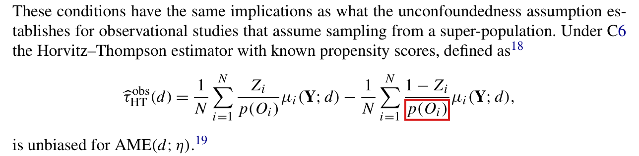
DOI
10.1214/24-AOAS1986
arXiv
2010.13599
Audited edition
Annals of Applied Statistics, 2025, 19(1):744–768; 25 pages in the audited file
SHA-256 of the audited file
decbf0e0589295a10ab2e2c596d0b20e1dbbfd0a51d71181854195aa8b8e833f
Permanent address
https://pmaronow.github.io/llm-audit/works/P004/

Summary

The paper studies spatial experiments in which treatment at one location may affect outcomes elsewhere in unknown ways. It defines an average marginalized effect by distance from an intervention node, gives asymptotically normal estimators under local interference, and reanalyses two studies of forest conservation. 43 entries are classified as errors (10 Moderate, 33 Minor), and 6 are clarity notes. The main finding is P004-E001: with an estimated logistic propensity score, the supplement’s expansion of the weighted estimator and the variance estimators built on it can be wrong when propensities vary.

What was and was not checked

I checked the following results, subject to the corrections and limits noted below.

  • Proposition 1 and equations (4)–(9): the marginalisation, the circle averages and the definition of the AME are consistent, and the Horvitz–Thompson estimator is unbiased under Bernoulli assignment. I followed the proof and enumerated every assignment of two small designs with interference, a ring of seven nodes and a design of four nodes with interactions.
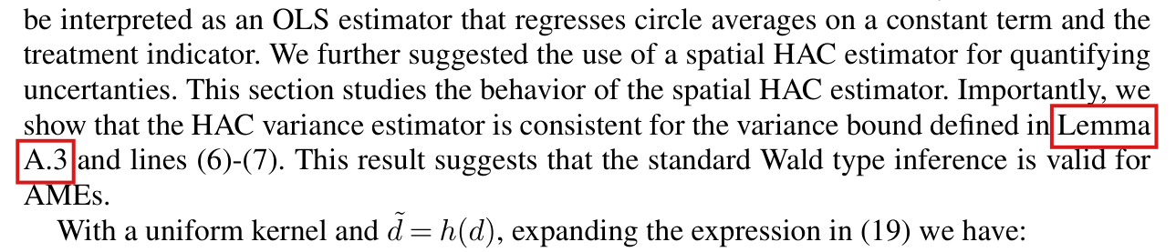
  • Supplement A, Lemma A.1 and Lemma A.2: the variance expansion and the bound O(1/N)O(1/N) under C1–C4, apart from the displays corrected in P004-N013.
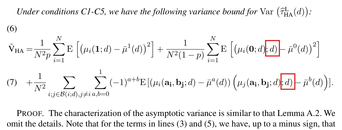
  • Lemma A.3 with the denominator corrected in P004-E011, and Lemma A.4: lines (2)–(5) equal the exact variance of the linearised Hajek estimator in an enumerated design, and lines (3) and (5) together equal −N−2∑i(τi−AME)∑j∈B(i)(τj−AME)-N^{-2}\sum_i(\tau_i-\mathrm{AME})\sum_{j\in\mathcal{B}(i)}(\tau_j-\mathrm{AME}).
  • Propositions 2 and 3: both include the lower bound on the scaled variance that a central limit theorem with a nondegenerate limit needs, and the argument through dependency neighbourhoods is sound under their premises. The restated Lemma A.5 is the subject of P004-E012.
  • Proposition 4 and Supplement A.4.1–A.4.3: the (2,2)(2,2) entry of the sandwich, the limit of the HAC estimator, the bias term under homophily, the bound behind the alternative variance estimator and the rescaling argument for conservative coverage with limits inferior as in P004-N024, apart from the other corrections recorded separately.
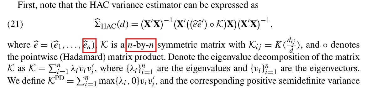
  • Equations (21)–(22) and footnotes 14–15: the truncated kernel is positive semidefinite and dominates the original kernel, and the positive semidefinite estimator is weakly larger.
  • Section 6.1, equations (23)–(25): under additivity the AME equals the average additive effect and does not depend on the design.
  • Supplement A.5: equation (32), equations (34)–(35), the comparison of the two estimators and the identity pΔ(1)=(1−p)Δ(0)p\Delta(1)=(1-p)\Delta(0) of its footnote 5.
  • Supplement A.6: the expansion of the maximum likelihood estimator of the logistic model in Lemma A.6, subject to P004-E003, and the Taylor expansion (42). The step that follows is the subject of P004-E001.
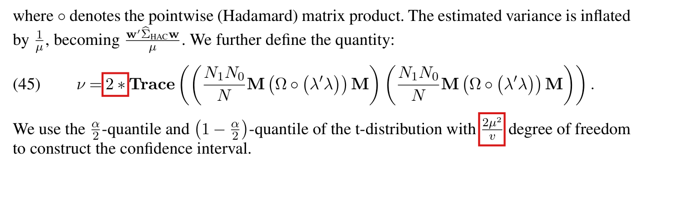
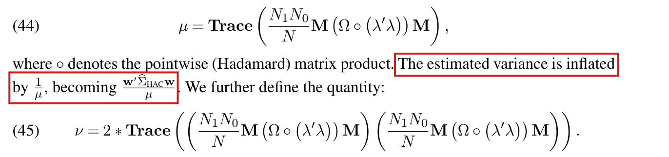
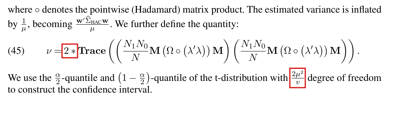
  • Supplement A.7, equations (44)–(45): the trace moments, and the degrees of freedom 2μ2/ν2\mu^2/\nu, which agree with the effective degrees of freedom of Satterthwaite and Young.
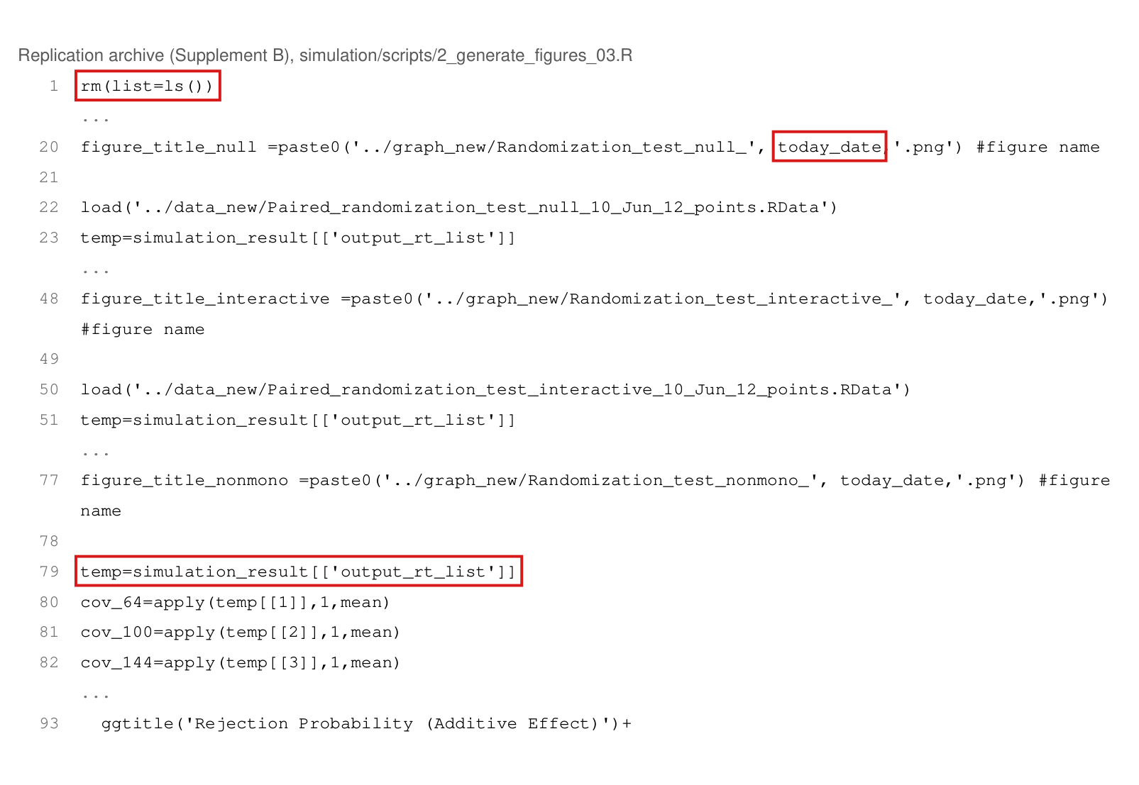
  • Randomization inference under the sharp null is valid for any fixed statistic when draws follow the experiment’s assignment law. The simulation code implements a two-sided test against 1,000 redraws, pointwise and for the supremum over the grid of footnote 23, and the images in the archive match Figure 9. The printed rejection rule is the subject of P004-E005.
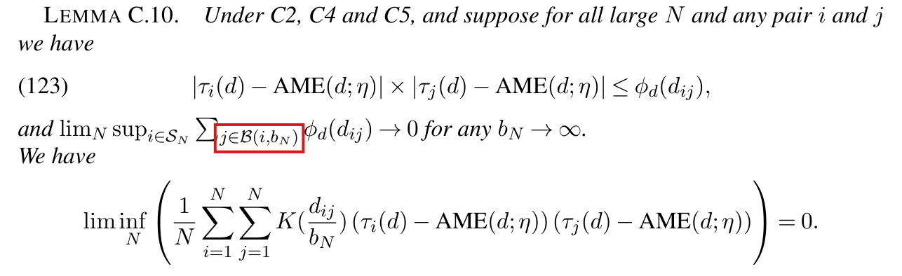
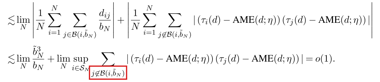
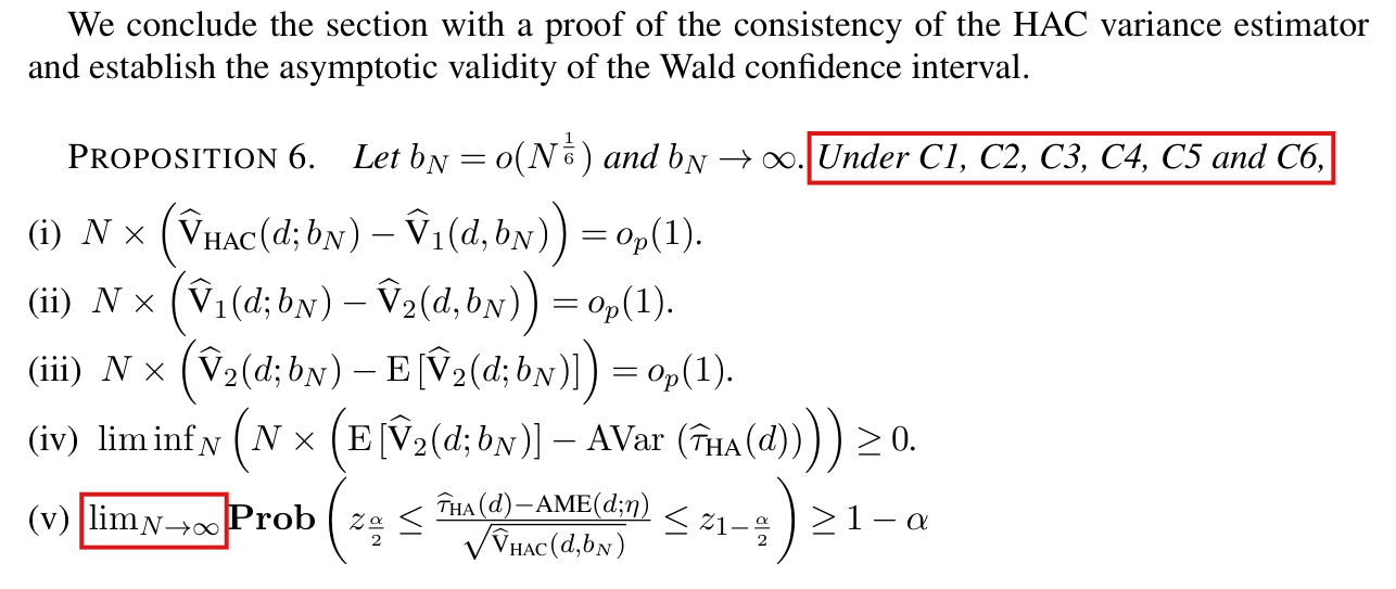
  • Supplement A, Appendix C: Lemmas C.1 and C.3, the counting bounds (69)–(74), Lemmas C.5–C.9, and Proposition 6 (i)–(iv) with the rate bN=o(N1/6)b_N=o(N^{1/6}) and the bound (150)–(155), after the corrections of printed expressions that are recorded separately. The hypothesis of Lemma C.10 is the subject of P004-E019.
  • Figure 3: the assignments listed in the text match the panels.
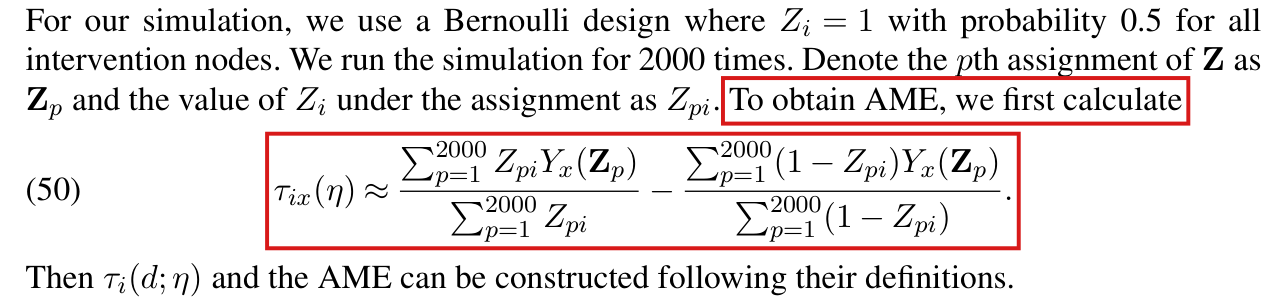
  • The simulation code agrees with Supplement B.1 in the numbers and layouts of nodes, the gamma densities, the interactive term, the 2,000 Bernoulli(0.5)(0.5) draws, the Monte Carlo AME of equation (50), the distance grid and the nominal HAC cutoff. The additive effect in the supplied code extends beyond its stated range, so that the justification for that cutoff fails (P004-E027).
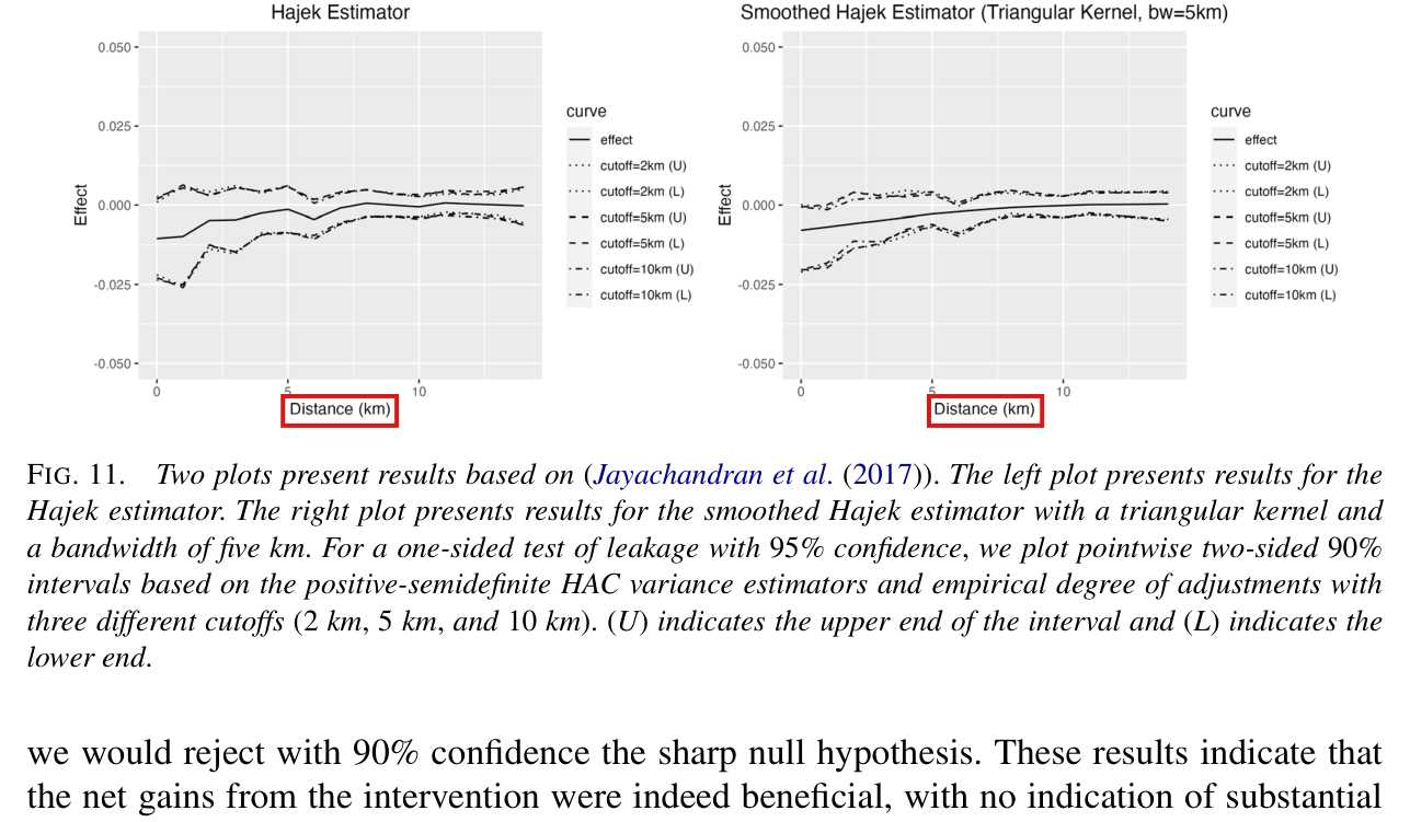
  • Uganda application: the stored data have 121 villages, 60 of them treated; the stored Hajek estimates equal differences in means recomputed from the stored circle averages; the kernel cutoff in the script matches footnote 25; and the intervals stored in the saved result object follow the normal 90% formula. A separate recalculation from the supplied raster gives a 0–5 km sum of −0.0427592-0.0427592 and a two-sided Monte Carlo fraction of 0.09280.0928, compared with the published −0.034-0.034 and approximately 0.0650.065 (P004-N006). Eight selected point estimates agree with Figure 11 at graph resolution; selected interval endpoints were compared, with the small lower-endpoint discrepancy described in P004-N006.
  • Costa Rica application: I reproduced the counts of 233 treated and 522 untreated tiles from the supplied data. All four selected smoothed point estimates agree with Figure 13 at graph resolution; three selected unsmoothed estimates and selected 2 km intervals exceed the graph-reading tolerances. I recalculated the full point-estimate grid but only selected interval endpoints.
  • The notation table of Supplement D agrees with the definitions of the article, apart from P004-N019. Among the 51 figures and five simulation images of the archive, no discrepancy was established beyond P004-N022 and P004-N023.

My checks had the following limits. The stored simulation results are not in the replication archive, so Figures 5–9, the simulation figures of the supplement and the rejection rate 0.056 could not be recomputed; I compared them only with the code that would produce them. The application scripts do not run as supplied (P004-E029); the recalculations for the two applications used the authors' functions on the supplied data, covered full point-estimate grids and selected interval endpoints, and were compared with readings of the published plots, which print no numerical values. I searched older variants of the simulation scripts and the package vignette for the relevant code. I consulted the original Uganda and Costa Rica studies for the assignment procedure and outcome date. The restated results in Lemma A.5 and the appeal to Theorem 2 of Jenish and Prucha (2012) were not compared with the originals. The article does not state the versions of R and of the spatial packages. The absence of further corrections does not establish that the rest of the paper is correct.

Headline claims and related corrections

  1. Under Bernoulli assignment with arbitrary, unspecified interference, the average marginalized effect AME⁡(d;η)\operatorname{AME}(d;\eta) is well defined and identified by randomization, and the Horvitz–Thompson contrast of circle averages is unbiased for it.

    Proposition 1; eqs. (4)-(14); Supplement A.1.1

  2. Under the Bernoulli design, bounded outcomes, local interference (C3) and node spacing (C4), and with scaled variances bounded below, the Horvitz–Thompson and Hajek estimators are N\sqrt{N}-consistent and asymptotically normal.

    Propositions 2 and 3; Lemmas A.2-A.5 of Supplement A

    See P004-E007, P004-E011, P004-E012, P004-N013, P004-N014, P004-N015.

  3. With the uniform kernel and cutoff h(d)h(d), the spatial HAC variance estimator gives asymptotically conservative Wald intervals for the Hajek estimator under a homophily condition (C5); the SAH bound estimator does so without C5; a positive semidefinite version of the HAC estimator is weakly larger.

    Proposition 4; eqs. (19)-(22); Supplement A.4 and A.7

    See P004-E013, P004-E016, P004-E024, P004-E025, P004-E026, P004-N004, P004-N014.

  4. When effects from different intervention nodes are additive, the AME does not depend on the assignment design and equals the average of the node-specific additive distance effects.

    Section 6.1; eqs. (23)-(25)

  5. The paper presents smoothed AMEs in equation (26), including disk and donut averages, and sharp-null randomization tests. In its simulations, pointwise rejection rates are close to 5%5\% under the null and approach one at distances with nonzero effects; the supremum-statistic test rejects in 5.6%5.6\% of null simulations and all additive and interactive simulations at N=64N=64.

    Sections 6.2-6.3; eq. (26); Section 7, Figure 9 and footnotes 22-23; Supplement B.1

    See P004-E005, P004-E006, P004-E022, P004-E030.

  6. The paper extends the framework to observational studies: the propensity-weighted Horvitz–Thompson estimator is unbiased under C6, and Section 6.4 claims a complete inferential theory for the IPW estimator with a logistic propensity model in Appendix A.6, including linearization, asymptotic normality, and HAC and SAH variance estimators.

    Section 6.4; Assumption C6; Supplement A.1.3 and A.6 (Lemma A.6, Proposition 4, eqs. (36)-(43))

    See P004-E001, P004-E002, P004-E003, P004-E004, P004-E014, P004-E015, P004-N016.

  7. Under its near-epoch dependence, spacing and variance assumptions, the paper extends N\sqrt{N}-consistency, asymptotic normality and consistency or conservativeness of the HAC estimator with a growing bandwidth to the Hajek estimator beyond local interference (C3).

    Section 6.5; footnote 5; Supplement Appendix C (Lemmas C.1-C.10, Propositions 5 and 6)

    See P004-E017, P004-E018, P004-E019, P004-E020, P004-E021, P004-N016, P004-N018.

  8. In simulations the Hajek estimator's MSE falls with the number of nodes; HAC intervals cover well at small distances and need the effective-degrees-of-freedom adjustment at large distances; the SAH interval is extremely conservative; the positive-semidefinite version costs little length; the recommended procedure is the positive-semidefinite HAC estimator with the effective-degrees-of-freedom adjustment.

    Section 7; Figures 5-8; Supplement B.1-B.3 (Figures 1-9); Supplement A.7

    See P004-E024, P004-E025, P004-E026, P004-E027, P004-N003, P004-N004.

  9. The Uganda reanalysis reports reduced deforestation inside treated villages, no indication of substantial leakage up to about 1515 km, and a randomization test on the summed 00–55 km estimates, with statistic −0.034-0.034 and a pp-value around 0.0650.065.

    Section 8.1; Figures 10-11; footnotes 24-25

    See P004-E007, P004-E008, P004-E029, P004-N005, P004-N006, P004-N007, P004-N009, P004-N011, P004-N022, P004-N023.

  10. Reanalysis of Costa Rica's protected areas as an observational study (233 treated and 522 untreated tiles, logistic propensity score on three covariates): deforestation diminished within protected areas and nearby, with no indication of substantial leakage.

    Section 8.2; Figures 12-13; Section 6.4; Supplement A.6

    See P004-E001, P004-E009, P004-E023, P004-E029, P004-N011.

Corrections

Moderate (10)

A real substantive error with limited reach.

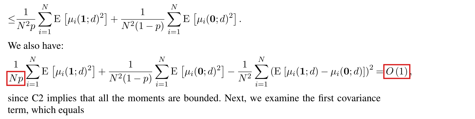
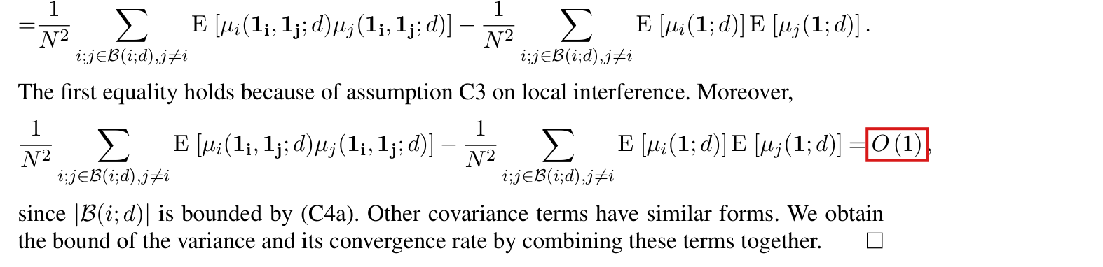
Equation (36) can fail when the assignment probabilities differ across nodes: to first order, estimating the logistic coefficient changes the IPW estimator by −N−1∑i(Zi−pi)Oi′γN-N^{-1}\sum_i(Z_i-p_i)O_i'\gamma_N with γN=HN−1N−1∑i[(1−pi)mi1+pimi0]Oi\gamma_N=H_N^{-1}N^{-1}\sum_i[(1-p_i)m_{i1}+p_im_{i0}]O_i, and the linear form, the variance, the two variance estimators and the coverage statements of Proposition 4 of A.6 are rebuilt on this term.

Supplement A, Appendix A.6: Proposition 4 and equation (36), p. 15; its proof, equations (42) and (43), p. 16, and the display after “Hence (42) becomes”, p. 17; condition C 2, p. 14. Announced in Section 6.4, p. 759 (PDF p. 16)

See also under Formal statements (Lean): P004-T1, P004-T2, P004-T4, P004-T35

As printed

Main text, Section 6.4, p. 759. In Appendix A.6, we develop a complete inferential theory for the inverse probability weighted (IPW) estimator where propensity scores are modeled using a logistic model.

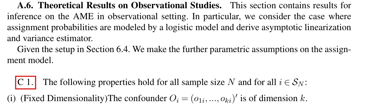
Supplement A, p. 14. For brevity, we denote p(Oi∣θ0)=p0(Oi)p(O_i\mid\theta_0)=p_0(O_i). We define the following coefficients:

β1,N=(1N∑i=1Np0(Oi)(1−p0(Oi))OiOi′)−1(1N∑i=1NE[μi(1;d) p0(Oi)(1−p0(Oi))Oi]),\beta_{1,N}=\Bigl(\frac1N\sum_{i=1}^{N}p_0(O_i)(1-p_0(O_i))O_iO_i'\Bigr)^{-1}\Bigl(\frac1N\sum_{i=1}^{N}\mathrm E\bigl[\mu_i(1;d)\,p_0(O_i)(1-p_0(O_i))O_i\bigr]\Bigr),

and,

β0,N=(1N∑i=1Np0(Oi)(1−p0(Oi))OiOi′)−1(1N∑i=1NE[μi(0;d) p0(Oi)(1−p0(Oi))Oi]).\beta_{0,N}=\Bigl(\frac1N\sum_{i=1}^{N}p_0(O_i)(1-p_0(O_i))O_iO_i'\Bigr)^{-1}\Bigl(\frac1N\sum_{i=1}^{N}\mathrm E\bigl[\mu_i(0;d)\,p_0(O_i)(1-p_0(O_i))O_i\bigr]\Bigr).

Supplement A, p. 15. Proposition 4. Define:

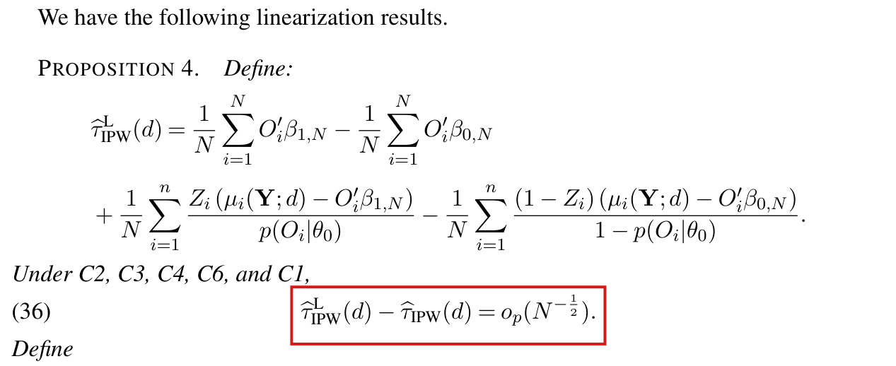
τ^IPWL(d)=1N∑i=1NOi′β1,N−1N∑i=1NOi′β0,N+1N∑i=1nZi(μi(Y;d)−Oi′β1,N)p(Oi∣θ0)−1N∑i=1n(1−Zi)(μi(Y;d)−Oi′β0,N)1−p(Oi∣θ0).\begin{aligned} \widehat\tau^{\mathrm{L}}_{\mathrm{IPW}}(d)={}&\frac1N\sum_{i=1}^{N}O_i'\beta_{1,N}-\frac1N\sum_{i=1}^{N}O_i'\beta_{0,N}\\ &+\frac1N\sum_{i=1}^{n}\frac{Z_i\bigl(\mu_i(\mathbf Y;d)-O_i'\beta_{1,N}\bigr)}{p(O_i\mid\theta_0)}-\frac1N\sum_{i=1}^{n}\frac{(1-Z_i)\bigl(\mu_i(\mathbf Y;d)-O_i'\beta_{0,N}\bigr)}{1-p(O_i\mid\theta_0)}. \end{aligned}

Under C2, C3, C4, C6, and C1,

τ^IPWL(d)−τ^IPW(d)=op(N−12).\widehat\tau^{\mathrm{L}}_{\mathrm{IPW}}(d)-\widehat\tau_{\mathrm{IPW}}(d)=\colorbox{#ffe58a}{$\displaystyle o_p(N^{-\frac12})$}.

Supplement A, proof, pp. 16–17, equation (43) and the next display.

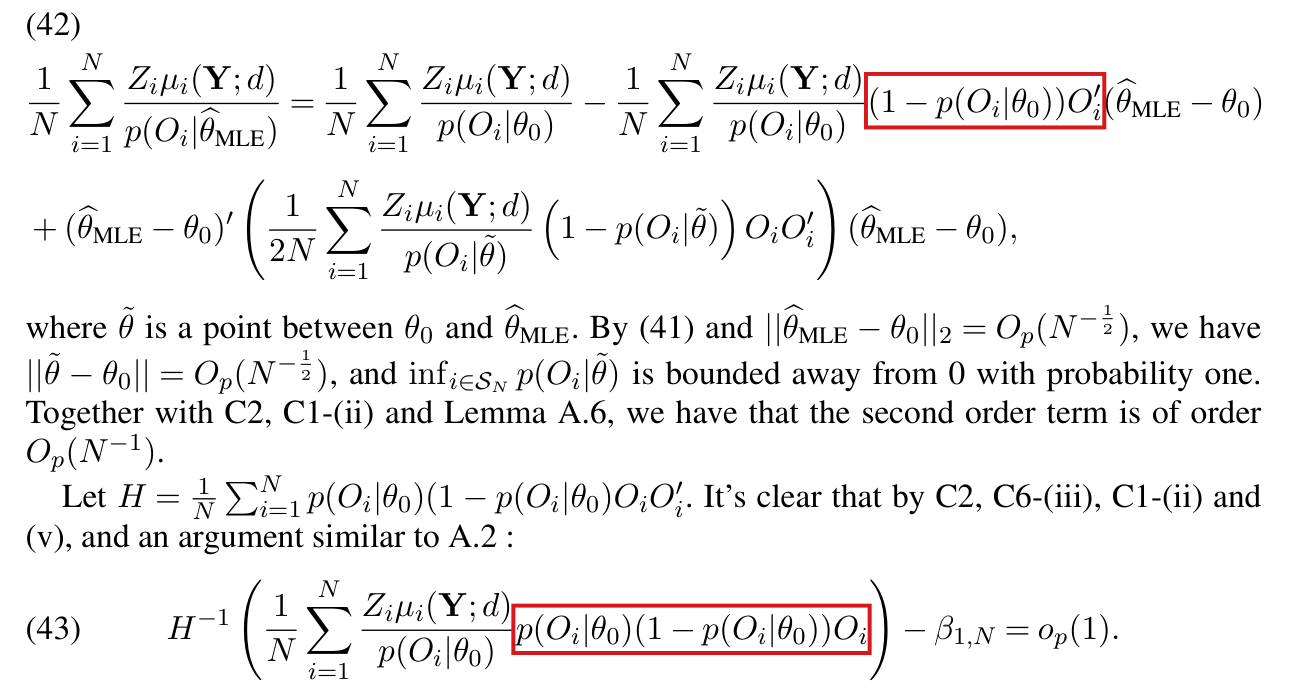
H−1(1N∑i=1NZiμi(Y;d)p(Oi∣θ0) p(Oi∣θ0)(1−p(Oi∣θ0))Oi)−β1,N=op(1).H^{-1}\Bigl(\frac1N\sum_{i=1}^{N}\frac{Z_i\mu_i(\mathbf Y;d)}{p(O_i\mid\theta_0)}\,p(O_i\mid\theta_0)(1-p(O_i\mid\theta_0))O_i\Bigr)-\beta_{1,N}=o_p(1).

Hence (42) becomes

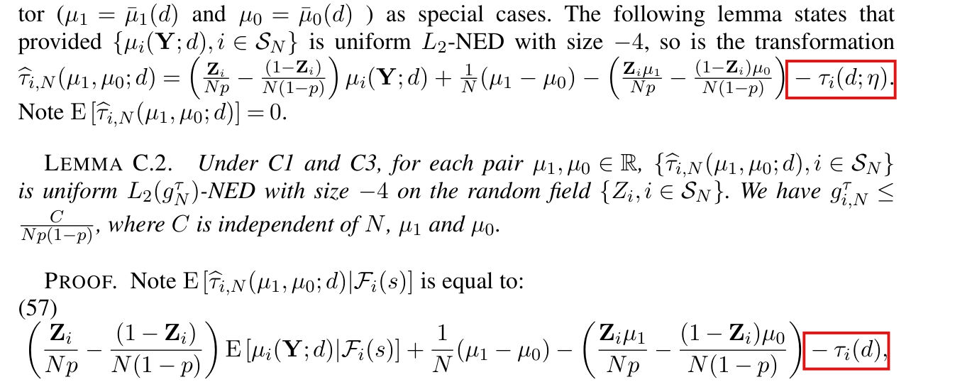
1N∑i=1NZiμi(Y;d)p(Oi∣θ^MLE)=1N∑i=1NZiμi(Y;d)p(Oi∣θ0)−1N∑i=1NZi−p(Oi∣θ0)p(Oi∣θ0)Oi′β1,N+op(N−12).\frac1N\sum_{i=1}^{N}\frac{Z_i\mu_i(\mathbf Y;d)}{p(O_i\mid\widehat\theta_{\mathrm{MLE}})}=\frac1N\sum_{i=1}^{N}\frac{Z_i\mu_i(\mathbf Y;d)}{p(O_i\mid\theta_0)}\colorbox{#ffe58a}{$\displaystyle -\frac1N\sum_{i=1}^{N}\frac{Z_i-p(O_i\mid\theta_0)}{p(O_i\mid\theta_0)}O_i'\beta_{1,N}$}+o_p(N^{-\frac12}).

Supplement A, p. 14, condition C 2. For all sample size NN,

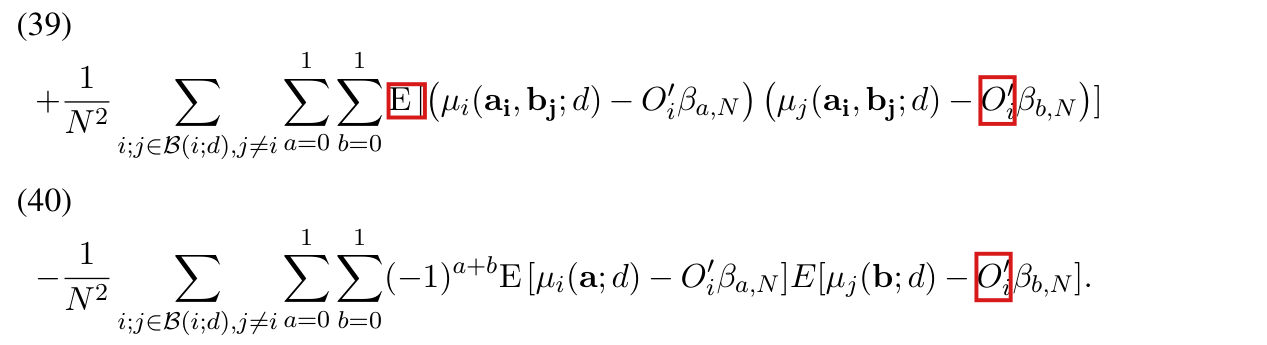
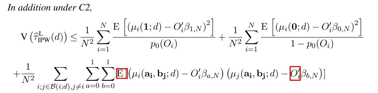
1N∑i=1N(τi(d;η)−(Oi′β1,N−Oi′β0,N))∑j∈B(i;d)(τj(d;η)−(Oi′β1,N−Oi′β0,N))≥0.\frac1N\sum_{i=1}^{N}\Bigl(\tau_i(d;\eta)-\bigl(O_i'\beta_{1,N}-O_i'\beta_{0,N}\bigr)\Bigr)\sum_{j\in\mathcal B(i;d)}\Bigl(\tau_j(d;\eta)-\bigl(\colorbox{#ffe58a}{$\displaystyle O_i'$}\beta_{1,N}-\colorbox{#ffe58a}{$\displaystyle O_i'$}\beta_{0,N}\bigr)\Bigr)\ge0.
The problem

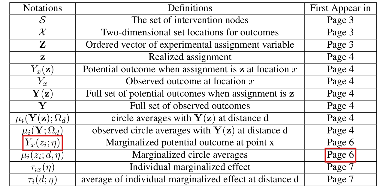
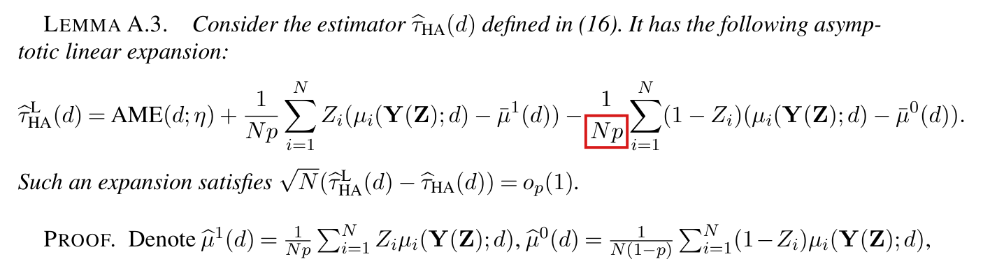
Throughout, dd is fixed, and I write Ri=μi(Y;d)R_i=\mu_i(\mathbf Y;d), pi=p(Oi∣θ0)p_i=p(O_i\mid\theta_0), mia=E[μi(a;d)]m_{ia}=E[\mu_i(a;d)] for a∈{0,1}a\in\{0,1\}, τi=mi1−mi0\tau_i=m_{i1}-m_{i0} and δi=Oi′(β1,N−β0,N)\delta_i=O_i'(\beta_{1,N}-\beta_{0,N}). Let

HN=1N∑i=1Npi(1−pi)OiOi′,SN=1N∑i=1N(Zi−pi)Oi,τ^HT=1N∑i=1N[ZiRipi−(1−Zi)Ri1−pi],H_N=\frac1N\sum_{i=1}^{N}p_i(1-p_i)O_iO_i',\qquad S_N=\frac1N\sum_{i=1}^{N}(Z_i-p_i)O_i,\qquad\widehat\tau_{HT}=\frac1N\sum_{i=1}^{N}\Bigl[\frac{Z_iR_i}{p_i}-\frac{(1-Z_i)R_i}{1-p_i}\Bigr],

so that βa,N=HN−1N−1∑ipi(1−pi)miaOi\beta_{a,N}=H_N^{-1}N^{-1}\sum_ip_i(1-p_i)m_{ia}O_i. The upper limits nn in the two residual sums of the proposition are read as NN, and “C1” in its hypotheses is the condition C 1 of A.6 (see P004-N016).

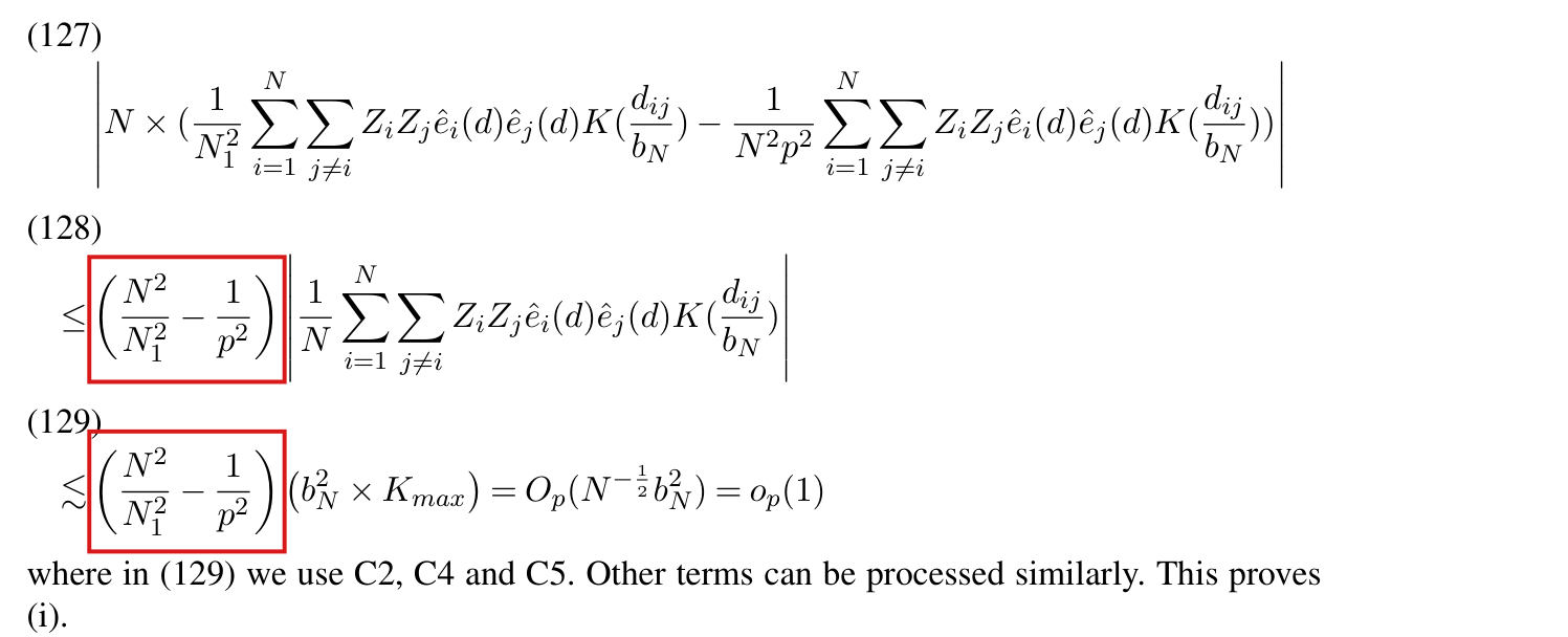
The first-order term of the expansion (42) has the coefficient N−1∑iZiRi(1−pi)Oi′/piN^{-1}\sum_iZ_iR_i(1-p_i)O_i'/p_i, whose expectation is N−1∑i(1−pi)mi1Oi′N^{-1}\sum_i(1-p_i)m_{i1}O_i'. Equation (43) concerns a different sum, in which ZiRi/piZ_iR_i/p_i is multiplied by pi(1−pi)Oip_i(1-p_i)O_i and not by (1−pi)Oi(1-p_i)O_i, and it is this sum that converges to HNβ1,NH_N\beta_{1,N}. The display after “Hence (42) becomes” puts β1,N\beta_{1,N} in place of the coefficient of (42) and moves a factor 1/pi1/p_i into the score sum. Lemma A.6 expresses θ^MLE−θ0\widehat\theta_{MLE}-\theta_0 through HN−1SNH_N^{-1}S_N, in which every node has the same weight, so no factor 1/pi1/p_i can arise there. The two expressions agree when all pip_i are equal and differ in general. Expanding the definition, I find that the printed linear form is

τ^IPWL=τ^HT−1N∑i=1N(Zi−pi)[Oi′β1,Npi+Oi′β0,N1−pi],\widehat\tau^{L}_{IPW}=\widehat\tau_{HT}-\frac1N\sum_{i=1}^{N}(Z_i-p_i)\Bigl[\frac{O_i'\beta_{1,N}}{p_i}+\frac{O_i'\beta_{0,N}}{1-p_i}\Bigr],

whereas the IPW estimator satisfies τ^IPW=τ^HT−SN′γN+Op(N−1)\widehat\tau_{IPW}=\widehat\tau_{HT}-S_N'\gamma_N+O_p(N^{-1}) with γN\gamma_N as in the headline. In general the two differ at order N−1/2N^{-1/2}, and then (36) fails. The variance calculation (37)–(40) is based on the printed linear form rather than the correct first-order form of the IPW estimator; the HAC and SAH estimators built on the residuals Ri−Oi′β^a,NR_i-O_i'\widehat\beta_{a,N} can estimate the wrong quantity, and the normal limit and the two coverage statements for the IPW estimator do not follow. As printed, Appendix A.6 does not supply the inferential theory that Section 6.4 announces.

Evidence an exact counterexample

The evidence is an exact counterexample to (36), computed in rational arithmetic, and a derivation of the corrected statement.

The expansion of the IPW estimator. For fixed outcomes and assignments,

∇θ ZiRip(Oi∣θ)=−ZiRi (1−p(Oi∣θ))p(Oi∣θ) Oi,∇θ[−(1−Zi)Ri1−p(Oi∣θ)]=−(1−Zi)Ri p(Oi∣θ)1−p(Oi∣θ) Oi.\nabla_\theta\,\frac{Z_iR_i}{p(O_i\mid\theta)}=-\frac{Z_iR_i\,(1-p(O_i\mid\theta))}{p(O_i\mid\theta)}\,O_i,\qquad\nabla_\theta\Bigl[-\frac{(1-Z_i)R_i}{1-p(O_i\mid\theta)}\Bigr]=-\frac{(1-Z_i)R_i\,p(O_i\mid\theta)}{1-p(O_i\mid\theta)}\,O_i.

Since ZiZ_i is independent of the other assignments, I have E[ZiRi]=pimi1E[Z_iR_i]=p_im_{i1} and E[(1−Zi)Ri]=(1−pi)mi0E[(1-Z_i)R_i]=(1-p_i)m_{i0}. The expected gradient of τ^IPW\widehat\tau_{IPW} at θ0\theta_0 is therefore −DN-D_N, where DN=N−1∑i[(1−pi)mi1+pimi0]OiD_N=N^{-1}\sum_i[(1-p_i)m_{i1}+p_im_{i0}]O_i. Under C2, C3, C4, C6 and C 1, the summands are bounded and each shares assignments with a bounded number of others, which implies that the gradient differs from −DN-D_N by Op(N−1/2)O_p(N^{-1/2}). The second derivatives are bounded near θ0\theta_0. Inserting the expansion θ^MLE−θ0=HN−1SN+Op(N−1)\widehat\theta_{MLE}-\theta_0=H_N^{-1}S_N+O_p(N^{-1}) from the logistic score equation, with θ0\theta_0 an interior point (P004-E003), I obtain τ^IPW=τ^HT−SN′γN+Op(N−1)\widehat\tau_{IPW}=\widehat\tau_{HT}-S_N'\gamma_N+O_p(N^{-1}) with γN=HN−1DN\gamma_N=H_N^{-1}D_N.

The counterexample. Let N=3KN=3K. The nodes are the points (10i,0)(10i,0), i=1,…,Ni=1,\dots,N, and the outcome points are the same points, so that at d=0d=0 the circle average of a node is the outcome at its own point. The nodes have the types t=−1,0,1t=-1,0,1, repeated in this order. A node of type tt has Ot=(1,t)′O_t=(1,t)' and the outcome qtq_t at its own point under every assignment, with q−1=1q_{-1}=1, q0=21/20q_0=21/20 and q1=1q_1=1. The assignments are independent with θ0=(0,log⁡2)′\theta_0=(0,\log2)' and Θ0=[−2,2]2\Theta_0=[-2,2]^2. Then pt=2t/(1+2t)p_t=2^t/(1+2^t), that is, 1/31/3, 1/21/2 and 2/32/3. Every hypothesis of the proposition holds. The outcomes are bounded. There is no interference, and B(i;0)={i}\mathcal B(i;0)=\{i\}. The nodes are 10 apart, the probabilities lie in (1/10,9/10)(1/10,9/10), the Gram matrix of the confounders is diag⁡(1,2/3)\operatorname{diag}(1,2/3), and θ0\theta_0 is an interior point of Θ0\Theta_0. Further, τi=0\tau_i=0 and β1,N=β0,N\beta_{1,N}=\beta_{0,N}, which implies that the sum in C 2 is 0, in the printed form and in the corrected one. The variance condition of the proposition also holds, since VP>0V_P>0 below. A direct computation gives

HN=diag⁡(25108,427),β1,N=β0,N=(509500,0)′,γN=(549125,0)′.H_N=\operatorname{diag}\Bigl(\frac{25}{108},\frac{4}{27}\Bigr),\qquad\beta_{1,N}=\beta_{0,N}=\Bigl(\frac{509}{500},0\Bigr)',\qquad\gamma_N=\Bigl(\frac{549}{125},0\Bigr)'.

Since the two arms have the same outcome, both linear forms are averages over the nodes of multiples of Zi−piZ_i-p_i. At a node of type tt, the first-order form of the IPW estimator has the coefficient ata_t and the printed linear form has the coefficient btb_t, where

at=qtpt(1−pt)−Ot′γN,bt=qt−Ot′β1,Npt(1−pt).a_t=\frac{q_t}{p_t(1-p_t)}-O_t'\gamma_N,\qquad b_t=\frac{q_t-O_t'\beta_{1,N}}{p_t(1-p_t)}.
The three types of node and the coefficient of Zi−piZ_i-p_i in the two linear forms.
Type ttptp_tqtq_tIPW estimator, ata_tPrinted linear form, btb_t
−1-11/31/31127/25027/250−81/1000-81/1000
001/21/221/2021/20−24/125-24/12516/12516/125
112/32/31127/25027/250−81/1000-81/1000

Note that the two sets of coefficients have opposite signs. Writing wt=pt(1−pt)w_t=p_t(1-p_t), I find that NN times the variances of the two linear forms and their difference are

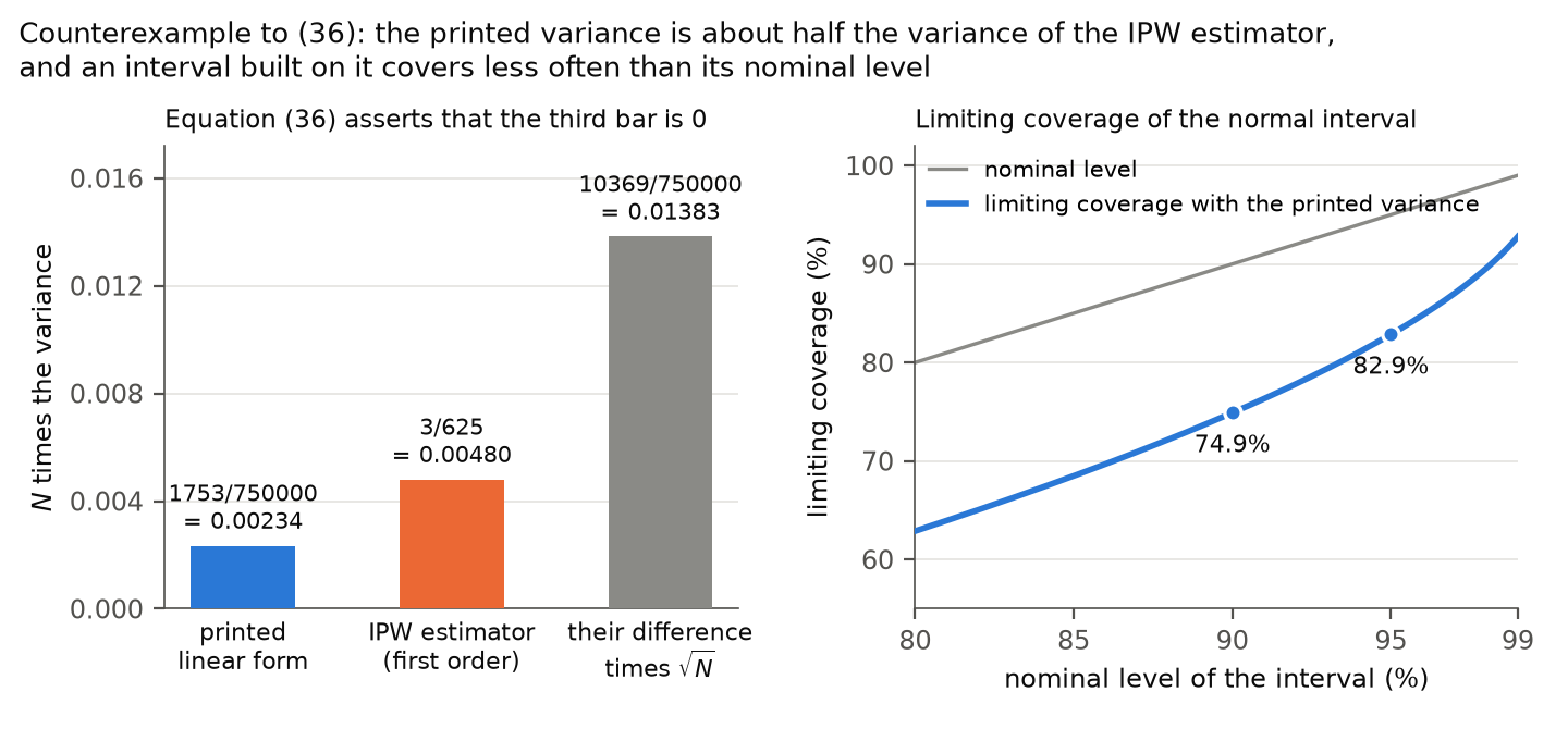
VA=13∑twtat2=3625,VP=13∑twtbt2=1753750000,VD=13∑twt(at−bt)2=10369750000V_A=\frac13\sum_tw_ta_t^2=\frac{3}{625},\qquad V_P=\frac13\sum_tw_tb_t^2=\frac{1753}{750000},\qquad V_D=\frac13\sum_tw_t(a_t-b_t)^2=\frac{10369}{750000}

for the first-order form of the IPW estimator, for the printed linear form, and for their difference, respectively. By the expansion above, N(τ^IPW−τ^IPWL)=UK+op(1)\sqrt N(\widehat\tau_{IPW}-\widehat\tau^{L}_{IPW})=U_K+o_p(1), where UKU_K is a normalized sum of KK independent and identically distributed terms, one for each block of three nodes. Its second moment is VDV_D and its fourth moment is at most 2205448981/22500000000002205448981/2250000000000 for every KK. By the Cauchy–Schwarz inequality, I have

Pr⁡(UK2>VD/2)≥1075161612205448981for every K≥1.\Pr\bigl(U_K^2>V_D/2\bigr)\ge\frac{107516161}{2205448981}\quad\text{for every }K\ge1.

Hence the difference in (36) is not op(N−1/2)o_p(N^{-1/2}). Further, N τ^IPW\sqrt N\,\widehat\tau_{IPW} converges in distribution to a normal variable with variance 3/6253/625, and the AME is 0. Then the ratio that Proposition 4 standardizes by the printed variance has limiting variance VA/VP=3600/1753V_A/V_P=3600/1753, not 1. In this example the printed HAC estimator, multiplied by NN, converges to VPV_P. A normal interval with critical value zz then has limiting coverage 2Φ(z1753/3600)−12\Phi(z\sqrt{1753/3600})-1, which is about 0.830.83 at the nominal level 0.950.95 and about 0.750.75 at the nominal level 0.900.90.

The corrected linear form. With Li=Oi′γNL_i=O_i'\gamma_N, the fits fi1f_{i1} and fi0f_{i0} of the corrected statement satisfy fi1−fi0=δif_{i1}-f_{i0}=\delta_i and fi1/pi+fi0/(1−pi)=Lif_{i1}/p_i+f_{i0}/(1-p_i)=L_i. For every assignment,

fi1−fi0−Zifi1pi+(1−Zi)fi01−pi=−(Zi−pi)[fi1pi+fi01−pi]=−(Zi−pi)Li.f_{i1}-f_{i0}-\frac{Z_if_{i1}}{p_i}+\frac{(1-Z_i)f_{i0}}{1-p_i}=-(Z_i-p_i)\Bigl[\frac{f_{i1}}{p_i}+\frac{f_{i0}}{1-p_i}\Bigr]=-(Z_i-p_i)L_i.

Summing over ii, I obtain N−1∑iδi+N−1∑iTi=τ^HT−SN′γNN^{-1}\sum_i\delta_i+N^{-1}\sum_iT_i=\widehat\tau_{HT}-S_N'\gamma_N as an identity, with TiT_i as in the corrected statement, and E[Ti]=τi−δiE[T_i]=\tau_i-\delta_i. The corrected form of (36) then follows from the expansion of the IPW estimator.

The variance estimators. Let VNV_N be the variance of N−1∑iTiN^{-1}\sum_iT_i, and let WW be the sum of the products TiTjT_iT_j over ii and j∈B(i;d)j\in\mathcal B(i;d), divided by N2N^2. By C3, the covariance of TiT_i and TjT_j vanishes when j∉B(i;d)j\notin\mathcal B(i;d), which implies that

E[W]=VN+1N2∑i=1N∑j∈B(i;d)(τi−δi)(τj−δj).E[W]=V_N+\frac{1}{N^2}\sum_{i=1}^{N}\sum_{j\in\mathcal B(i;d)}(\tau_i-\delta_i)(\tau_j-\delta_j).

The last sum is nonnegative under the corrected C 2, which is the homophily condition of the paper with OjO_j in its second factor. For the SAH estimator, the inequality Cov⁡(Ti,Tj)≤(Var⁡Ti+Var⁡Tj)/2\operatorname{Cov}(T_i,T_j)\le(\operatorname{Var}T_i+\operatorname{Var}T_j)/2 and the symmetry of the neighbourhoods give Var⁡(∑iTi)≤∑ici(d)E[Ti2]\operatorname{Var}(\sum_iT_i)\le\sum_ic_i(d)E[T_i^2], with no homophily condition, and Ti2T_i^2 is the bracket in the corrected SAH estimator. The TiT_i are bounded, and each depends on the assignments of a bounded number of nodes. By Chebyshev’s inequality, NN times each of the two sums concentrates around its expectation. The estimated fits f^ia\widehat f_{ia} are consistent uniformly in ii, since θ^MLE\widehat\theta_{MLE}, γ^\widehat\gamma and β^a,N\widehat\beta_{a,N} have errors of order N−1/2N^{-1/2}. Then replacing TiT_i by T^i\widehat T_i changes NN times each sum by op(1)o_p(1). Finally, a sum of bounded variables whose dependency graph has bounded degree is asymptotically normal when its variance is of order NN, which is the condition that NVNNV_N is bounded below.

Three remarks on the correction. First, the index in C 2 matters. In a second exact example, with three types on a path, the printed sum of C 2 equals 7/339>07/339>0 and the corrected sum equals −775/38307<0-775/38307<0. The corrected HAC estimator, multiplied by NN, then converges to 6053/1532286053/153228, below the value 27/45227/452 of NVNNV_N. Second, a positive printed variance does not imply that VNV_N is positive. With q=(1,9/8,1)q=(1,9/8,1) in the counterexample, the first-order form of the IPW estimator vanishes identically, while NN times the printed variance is 1753/1200001753/120000. Third, the fits are not unique. The fits gi1=piOi′γ1g_{i1}=p_iO_i'\gamma_1 and gi0=(1−pi)Oi′γ0g_{i0}=(1-p_i)O_i'\gamma_0, with γ1=HN−1N−1∑i(1−pi)mi1Oi\gamma_1=H_N^{-1}N^{-1}\sum_i(1-p_i)m_{i1}O_i and γ0=HN−1N−1∑ipimi0Oi\gamma_0=H_N^{-1}N^{-1}\sum_ip_im_{i0}O_i, yield the same linear form. With them, however, the bound for the HAC estimator needs homophily of τi−gi1+gi0\tau_i-g_{i1}+g_{i0}, which C 2 does not imply: in a third example the sum for gg equals −9/2000-9/2000 while the sum of C 2 is 0. The fits ff avoid this additional condition.

What is not established. Equation (36) does not fail in every design with unequal probabilities. With two types of node, a saturated logistic model and outcomes that depend only on the type and the arm, (36) holds although the probabilities differ. No published figure, estimate or interval of the observational application has been shown to change, and the corrected conditions have not been checked for that application.

What survives

The definition of the AME, its identification under independent assignment, and the Horvitz–Thompson estimator with known probabilities (with the weight corrected in P004-E004) are not affected. The theory of Sections 4 and 5 for experiments with a constant probability does not use Proposition 4 of A.6. The IPW estimator remains consistent for the AME. The defect concerns its first-order approximation and the variance derived from it. The printed expansion is correct when the logistic model has an intercept only, since all probabilities are then equal. What changes is the inference for the IPW estimator with a fitted logistic model: the linear form, its variance, the two variance estimators and the conditions are replaced as below. The correction keeps the estimand, the estimator and the homophily condition in its intended form. It adds two regularity conditions, an interior θ0\theta_0 and a positive lower bound on NN times the corrected variance.

Corrected

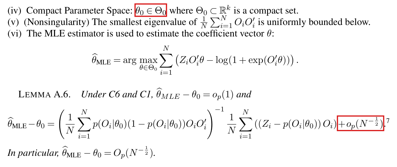
Condition C 1(iv). Θ0⊂Rk\Theta_0\subset\mathbb R^k is a fixed compact set, and θ0\theta_0 is an interior point of Θ0\Theta_0 (P004-E003).

Condition C 2. For all sample sizes NN, with δi=Oi′(β1,N−β0,N)\delta_i=O_i'(\beta_{1,N}-\beta_{0,N}),

1N∑i=1N∑j∈B(i;d)(τi(d;η)−δi)(τj(d;η)−δj)≥0.\frac1N\sum_{i=1}^{N}\sum_{j\in\mathcal B(i;d)}\bigl(\tau_i(d;\eta)-\delta_i\bigr)\bigl(\tau_j(d;\eta)-\colorbox{#ffe58a}{$\displaystyle \delta_j$}\bigr)\ge0 .

Here B(i;d)\mathcal B(i;d) is the neighbourhood (12), which contains ii (see also P004-E015).

Proposition 4 of A.6. Write pi=p(Oi∣θ0)p_i=p(O_i\mid\theta_0), mia=E[μi(a;d)]m_{ia}=E[\mu_i(a;d)] and HN=N−1∑ipi(1−pi)OiOi′H_N=N^{-1}\sum_ip_i(1-p_i)O_iO_i'. Define

γN=HN−1 1N∑i=1N[(1−pi)mi1+pimi0]Oi,Li=Oi′γN,\colorbox{#ffe58a}{$\displaystyle \gamma_N=H_N^{-1}\,\frac1N\sum_{i=1}^{N}\bigl[(1-p_i)m_{i1}+p_im_{i0}\bigr]O_i$},\qquad L_i=O_i'\gamma_N,
fi1=piδi+pi(1−pi)Li,fi0=−(1−pi)δi+pi(1−pi)Li,\colorbox{#ffe58a}{$\displaystyle f_{i1}=p_i\delta_i+p_i(1-p_i)L_i$},\qquad\colorbox{#ffe58a}{$\displaystyle f_{i0}=-(1-p_i)\delta_i+p_i(1-p_i)L_i$},
τ^IPWL(d)=1N∑i=1Nδi+1N∑i=1NTi,Ti=Zi(μi(Y;d)−fi1)pi−(1−Zi)(μi(Y;d)−fi0)1−pi.\widehat\tau^{L}_{IPW}(d)=\frac1N\sum_{i=1}^{N}\delta_i+\frac1N\sum_{i=1}^{N}T_i,\qquad T_i=\frac{Z_i\bigl(\mu_i(\mathbf Y;d)-\colorbox{#ffe58a}{$\displaystyle f_{i1}$}\bigr)}{p_i}-\frac{(1-Z_i)\bigl(\mu_i(\mathbf Y;d)-\colorbox{#ffe58a}{$\displaystyle f_{i0}$}\bigr)}{1-p_i}.

Under C2, C3, C4, C6 and C 1 with item (iv) as above,

τ^IPWL(d)−τ^IPW(d)=op(N−12).\widehat\tau^{L}_{IPW}(d)-\widehat\tau_{IPW}(d)=o_p(N^{-\frac12}).

The variance VN=V(τ^IPWL(d))V_N=V(\widehat\tau^{L}_{IPW}(d)) is

VN=1N2∑i=1N{E[(μi(1;d)−fi1)2]pi+E[(μi(0;d)−fi0)2]1−pi}+1N2∑i; j∈B(i;d), j≠i ∑a=01∑b=01(−1)a+bE[(μi(ai,bj;d)−fia)(μj(ai,bj;d)−fjb)]−1N2∑i=1N∑j∈B(i;d)(τi−δi)(τj−δj).\begin{aligned} V_N={}&\frac{1}{N^2}\sum_{i=1}^{N}\Bigl\{\frac{E\bigl[(\mu_i(\mathbf 1;d)-f_{i1})^2\bigr]}{p_i}+\frac{E\bigl[(\mu_i(\mathbf 0;d)-f_{i0})^2\bigr]}{1-p_i}\Bigr\}\\ &+\frac{1}{N^2}\sum_{i;\,j\in\mathcal B(i;d),\,j\ne i}\ \sum_{a=0}^{1}\sum_{b=0}^{1}(-1)^{a+b}E\bigl[\bigl(\mu_i(\mathbf a_i,\mathbf b_j;d)-f_{ia}\bigr)\bigl(\mu_j(\mathbf a_i,\mathbf b_j;d)-f_{jb}\bigr)\bigr]\\ &-\frac{1}{N^2}\sum_{i=1}^{N}\sum_{j\in\mathcal B(i;d)}(\tau_i-\delta_i)(\tau_j-\delta_j). \end{aligned}

If N×VNN\times V_N is uniformly bounded below by a positive constant for all large NN, then

τ^IPW(d)−AME(d;η)VN→dN(0,1).\frac{\widehat\tau_{IPW}(d)-\mathrm{AME}(d;\eta)}{\sqrt{V_N}}\xrightarrow{d}N(0,1).

Let p^i=p(Oi∣θ^MLE)\widehat p_i=p(O_i\mid\widehat\theta_{MLE}), H^=N−1∑ip^i(1−p^i)OiOi′\widehat H=N^{-1}\sum_i\widehat p_i(1-\widehat p_i)O_iO_i', and

γ^=H^−1 1N∑i=1N[Ziμi(Y;d)(1−p^i)p^i+(1−Zi)μi(Y;d) p^i1−p^i]Oi.\widehat\gamma=\widehat H^{-1}\,\frac1N\sum_{i=1}^{N}\Bigl[\frac{Z_i\mu_i(\mathbf Y;d)(1-\widehat p_i)}{\widehat p_i}+\frac{(1-Z_i)\mu_i(\mathbf Y;d)\,\widehat p_i}{1-\widehat p_i}\Bigr]O_i .

Let β^1,N\widehat\beta_{1,N} and β^0,N\widehat\beta_{0,N} be as in footnote 9 of the supplement, δ^i=Oi′(β^1,N−β^0,N)\widehat\delta_i=O_i'(\widehat\beta_{1,N}-\widehat\beta_{0,N}) and L^i=Oi′γ^\widehat L_i=O_i'\widehat\gamma, and let f^i1\widehat f_{i1}, f^i0\widehat f_{i0} and T^i\widehat T_i be defined as fi1f_{i1}, fi0f_{i0} and TiT_i with p^i\widehat p_i, δ^i\widehat\delta_i and L^i\widehat L_i in place of pip_i, δi\delta_i and LiL_i. Define

V^HACobs(d)=1N2∑i=1N∑j∈B(i;d)T^iT^j,V^SAHobs(d)=1N2∑i=1Nci(d)[Zi(μi(Y;d)−f^i1)2p^i 2+(1−Zi)(μi(Y;d)−f^i0)2(1−p^i)2].\begin{aligned} \widehat V^{obs}_{HAC}(d)&=\frac{1}{N^2}\sum_{i=1}^{N}\sum_{j\in\mathcal B(i;d)}\widehat T_i\widehat T_j,\\ \widehat V^{obs}_{SAH}(d)&=\frac{1}{N^2}\sum_{i=1}^{N}c_i(d)\Bigl[\frac{Z_i\bigl(\mu_i(\mathbf Y;d)-\widehat f_{i1}\bigr)^2}{\widehat p_i^{\,2}}+\frac{(1-Z_i)\bigl(\mu_i(\mathbf Y;d)-\widehat f_{i0}\bigr)^2}{(1-\widehat p_i)^2}\Bigr]. \end{aligned}

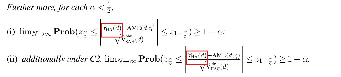
Then, for each 0<α<1/2\colorbox{#ffe58a}{$0<$}\alpha<1/2,

lim inf⁡N→∞Pr⁡(∣τ^IPW(d)−AME(d;η)∣≤z1−α/2V^SAHobs(d))≥1−α,\liminf_{N\to\infty}\Pr\Bigl(\bigl|\widehat\tau_{IPW}(d)-\mathrm{AME}(d;\eta)\bigr|\le z_{1-\alpha/2}\sqrt{\widehat V^{obs}_{SAH}(d)}\Bigr)\ge1-\alpha,

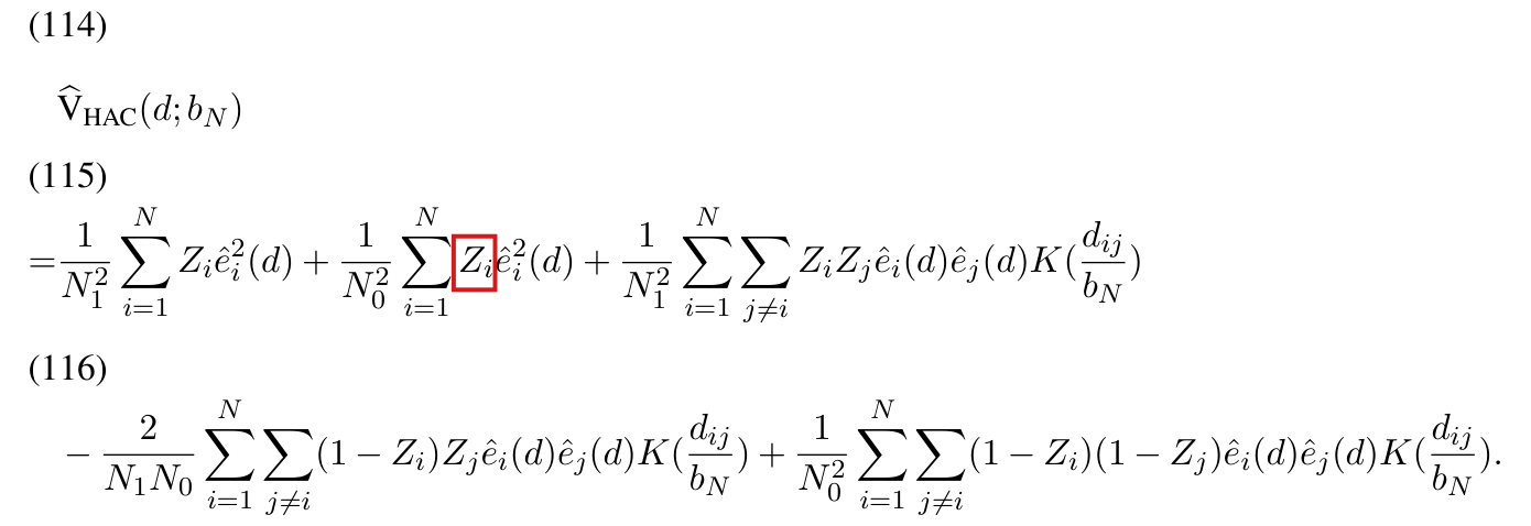
and, additionally under C 2 as corrected above, the same inequality holds with max⁡{V^HACobs(d),0}\colorbox{#ffe58a}{$\max\{\widehat V^{obs}_{HAC}(d),0\}$} in place of V^SAHobs(d)\widehat V^{obs}_{SAH}(d). When both assignment arms are nonempty, the estimator V^HACobs(d)\widehat V^{obs}_{HAC}(d) is the (2,2) entry of the sandwich printed on p. 15 when the residual there is taken to be

ϵ^i=N1N Zi(μi(Y;d)−f^i1)p^i+N0N (1−Zi)(μi(Y;d)−f^i0)1−p^i.\widehat\epsilon_i=\frac{N_1}{N}\,\frac{Z_i\bigl(\mu_i(\mathbf Y;d)-\widehat f_{i1}\bigr)}{\widehat p_i}+\frac{N_0}{N}\,\frac{(1-Z_i)\bigl(\mu_i(\mathbf Y;d)-\widehat f_{i0}\bigr)}{1-\widehat p_i}.

In V^SAHobs(d)\widehat V^{obs}_{SAH}(d) the residuals μi(Y;d)−f^ia\mu_i(\mathbf Y;d)-\widehat f_{ia} are not weighted before they are squared, so that the inverse probability enters once, squared (see P004-E002).

Main text, Section 6.4, p. 759. The sentence stands with this proposition in place of the printed one.

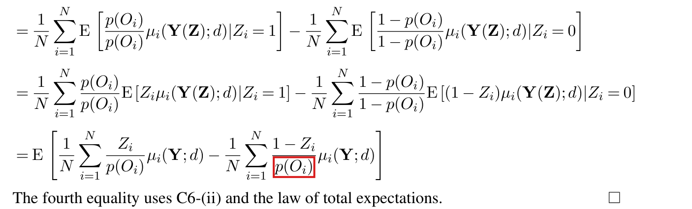
Crop of the start of Proposition 4. After the words We have the following linearization results and Proposition 4. Define, a two-line display defines tau-hat-L sub IPW of d as the average of O sub i prime beta sub 1,N minus the average of O sub i prime beta sub 0,N, plus the average of Z sub i times mu sub i of Y and d minus O sub i prime beta sub 1,N, over p of O sub i given theta-zero, minus the average of 1 minus Z sub i times mu sub i of Y and d minus O sub i prime beta sub 0,N, over 1 minus p of O sub i given theta-zero. The two last sums have the upper limit n. Then: Under C2, C3, C4, C6, and C1, equation (36): tau-hat-L sub IPW of d minus tau-hat sub IPW of d equals o-p of N to the minus one half. A red outline surrounds equation (36).
Supplement A, Proposition 4 of Appendix A.6, p. 15. The outline marks equation (36), which asserts that the printed linear form and the IPW estimator differ by op(N−1/2)o_p(N^{-1/2}).
Crop of equations (42) and (43) with the text between them. Equation (42) expands the average of Z sub i mu sub i over p of O sub i given theta-hat-MLE as the same average at theta-zero, minus the average of Z sub i mu sub i over p of O sub i given theta-zero, times 1 minus p of O sub i given theta-zero, times O sub i prime, times theta-hat-MLE minus theta-zero, plus a second-order term. Equation (43) states that H inverse times the average of Z sub i mu sub i over p of O sub i given theta-zero, times p of O sub i given theta-zero times 1 minus p of O sub i given theta-zero times O sub i, minus beta sub 1,N, is o-p of 1. One red outline surrounds the factor 1 minus p times O sub i prime in (42). A second surrounds the factor p times 1 minus p times O sub i in (43).
Supplement A, proof of Proposition 4, equations (42) and (43), p. 16. The outlines mark the weight (1−p(Oi∣θ0))Oi′(1-p(O_i\mid\theta_0))O_i' in the first-order term of (42) and the different weight p(Oi∣θ0)(1−p(Oi∣θ0))Oip(O_i\mid\theta_0)(1-p(O_i\mid\theta_0))O_i in (43).
Crop of one line of text and a displayed equation. The text reads: Hence (42) becomes. The equation states that the average of Z sub i mu sub i over p of O sub i given theta-hat-MLE equals the average of Z sub i mu sub i over p of O sub i given theta-zero, minus the average of Z sub i minus p of O sub i given theta-zero, over p of O sub i given theta-zero, times O sub i prime beta sub 1,N, plus o-p of N to the minus one half. A red outline surrounds the second term on the right, from its minus sign to beta sub 1,N.
Supplement A, proof of Proposition 4, top of p. 17. The outline marks the correction term that is substituted into (42).
Crop of a line of text, a heading and a displayed inequality. The text reads: A similar homophily condition is needed for the HAC variance estimation. C 2. For all sample size N. The inequality states that one over N times the sum over i of tau sub i minus the difference of O sub i prime beta sub 1,N and O sub i prime beta sub 0,N, times the sum over j in B of i and d of tau sub j minus the difference of O sub i prime beta sub 1,N and O sub i prime beta sub 0,N, is at least 0. Red outlines surround the two symbols O sub i prime in the second factor.
Supplement A, condition C 2, p. 14. The outlines mark the two places in the second factor where Oi′O_i' is printed and Oj′O_j' is needed.
Crop of five lines of text. They read: In practice, p of O sub i is unknown to researchers. In such cases, parametric methods, such as logistic regression, and nonparametric methods, such as the sieve estimator in Hirano, Imbens and Ridder (2003), can be used to estimate the propensity score. In Appendix A.6, we develop a complete inferential theory for the inverse probability weighted (IPW) estimator where propensity scores are modeled using a logistic model. A red outline surrounds the line that begins we develop a complete inferential theory.
Main text, Section 6.4, p. 759 (PDF p. 16). The outline marks the line that announces the theory of Appendix A.6.
Two panels under the title: Counterexample to (36): the printed variance is about half the variance of the IPW estimator, and an interval built on it covers less often than its nominal level. Left panel, three bars on an axis labelled N times the variance: a blue bar of height 1753/750000 = 0.00234 for N times the variance of the printed linear form, an orange bar of height 3/625 = 0.00480 for N times the variance of the IPW estimator to first order, and a grey bar of height 10369/750000 = 0.01383 for the variance of their difference scaled by the square root of N. The panel is headed: Equation (36) asserts that the third bar is 0. Right panel, a line chart of limiting coverage in percent against the nominal level of the interval in percent, from 80 to 99: a grey straight line for the nominal level and a blue curve below it for the limiting coverage with the printed variance, with marked points 74.9 percent at nominal 90 and 82.9 percent at nominal 95.
The counterexample to (36). Left: NN times the variance of the printed linear form (1753/7500001753/750000) and of the first-order form of the IPW estimator (3/6253/625), and the variance of N\sqrt N times their difference (10369/75000010369/750000), which (36) asserts to vanish in the limit. Right: the limiting coverage 2Φ(z1753/3600)−12\Phi(z\sqrt{1753/3600})-1 of a normal interval for the IPW estimator whose variance estimate converges to the printed variance, against its nominal level.

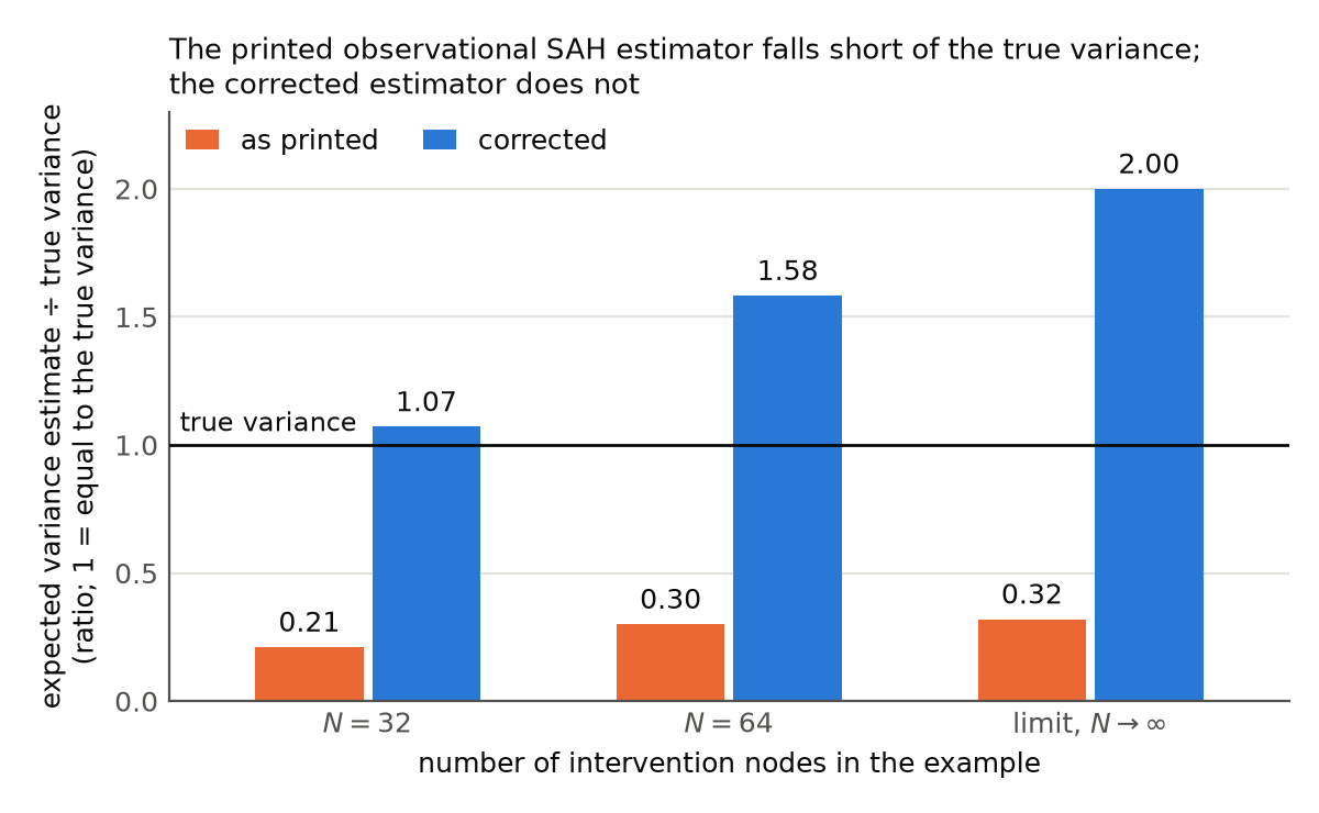
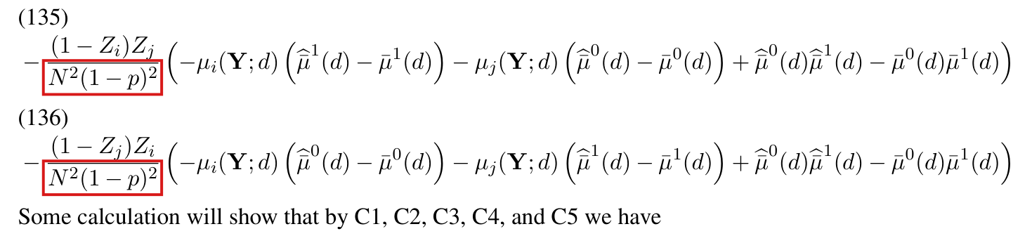
The observational SAH estimator divides the square of an inverse-propensity-weighted residual by the squared propensity a second time; the corrected estimator is N1−2∑iZici(d)ϵ^i2+N0−2∑i(1−Zi)ci(d)ϵ^i2N_1^{-2}\sum_iZ_ic_i(d)\widehat\epsilon_i^2+N_0^{-2}\sum_i(1-Z_i)c_i(d)\widehat\epsilon_i^2.

Supplement A, A.6, p. 15 (supplement PDF p. 15): the residual ϵ^i\widehat\epsilon_i and the display of V^SAHobs(d)\widehat V^{\mathrm{obs}}_{\mathrm{SAH}}(d)

See also under Formal statements (Lean): P004-T3, P004-T4, P004-T36

As printed

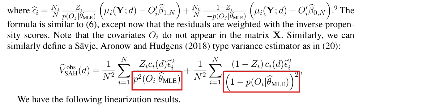
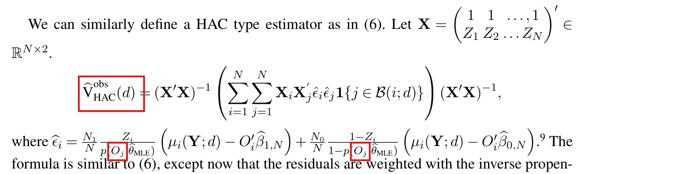
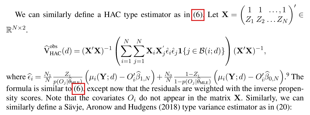
“where ϵ^i=N1NZip(Oj∣θ^MLE)(μi(Y;d)−Oi′β^1,N)+N0N1−Zi1−p(Oj∣θ^MLE)(μi(Y;d)−Oi′β^0,N)\widehat\epsilon_i=\frac{N_1}{N}\frac{Z_i}{p(\colorbox{#ffe58a}{$O_j$}|\widehat\theta_{\mathrm{MLE}})}\big(\mu_i(\mathbf Y;d)-O_i'\widehat\beta_{1,N}\big)+\frac{N_0}{N}\frac{1-Z_i}{1-p(\colorbox{#ffe58a}{$O_j$}|\widehat\theta_{\mathrm{MLE}})}\big(\mu_i(\mathbf Y;d)-O_i'\widehat\beta_{0,N}\big).9^{9} The formula is similar to (6), except now that the residuals are weighted with the inverse propensity scores. Note that the covariates OiO_i do not appear in the matrix X\mathbf X. Similarly, we can similarly define a Sävje, Aronow and Hudgens (2018) type variance estimator as in (20):

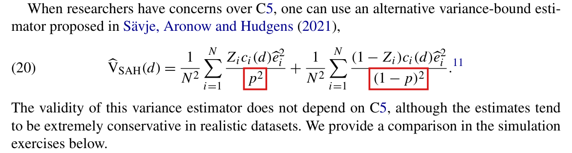
V^SAHobs(d)=1N2∑i=1NZici(d)ϵ^i2p2(Oi∣θ^MLE)+1N2∑i=1N(1−Zi) ci(d)ϵ^i2(1−p(Oi∣θ^MLE))2,”\widehat V^{\mathrm{obs}}_{\mathrm{SAH}}(d)=\frac1{N^2}\sum_{i=1}^N\frac{Z_ic_i(d)\widehat\epsilon_i^2}{\colorbox{#ffe58a}{$\displaystyle p^2(O_i|\widehat\theta_{\mathrm{MLE}})$}}+\frac1{N^2}\sum_{i=1}^N\frac{(1-Z_i)\,c_i(d)\widehat\epsilon_i^2}{\colorbox{#ffe58a}{$\displaystyle \big(1-p(O_i|\widehat\theta_{\mathrm{MLE}})\big)^2$}},\text{''}
The problem

The residual ϵ^i\widehat\epsilon_i defined above the display already contains the inverse propensity weight. I write p^i=p(Oi∣θ^MLE)\widehat p_i=p(O_i|\widehat\theta_{\mathrm{MLE}}) and r^ia=μi(Y;d)−Oi′β^a,N\widehat r_{ia}=\mu_i(\mathbf Y;d)-O_i'\widehat\beta_{a,N}, and I read the unbound OjO_j of the residual as OiO_i (see P004-E015). For a treated node, ϵ^i=(N1/N) r^i1/p^i\widehat\epsilon_i=(N_1/N)\,\widehat r_{i1}/\widehat p_i. The SAH display divides ϵ^i2\widehat\epsilon_i^2 by p^i2\widehat p_i^2 again. Substituting the residual into the display, I obtain

V^SAHobs(d)=1N2∑i=1Nci(d)[(N1N)2Zir^i12p^i 4+(N0N)2(1−Zi)r^i02(1−p^i)4],\widehat V^{\mathrm{obs}}_{\mathrm{SAH}}(d)=\frac1{N^2}\sum_{i=1}^Nc_i(d)\left[\Big(\frac{N_1}{N}\Big)^2\frac{Z_i\widehat r_{i1}^2}{\widehat p_i^{\,4}}+\Big(\frac{N_0}{N}\Big)^2\frac{(1-Z_i)\widehat r_{i0}^2}{(1-\widehat p_i)^4}\right],

whereas the analogue of (20) has Zir^i12/p^i 2Z_i\widehat r_{i1}^2/\widehat p_i^{\,2} and (1−Zi)r^i02/(1−p^i)2(1-Z_i)\widehat r_{i0}^2/(1-\widehat p_i)^2 in the brackets. The two differ by the factors (N1/(Np^i))2(N_1/(N\widehat p_i))^2 and (N0/(N(1−p^i)))2(N_0/(N(1-\widehat p_i)))^2. These factors equal 11 for an intercept-only logistic model with an interior maximum-likelihood estimate, where p^i=N1/N\widehat p_i=N_1/N, and they can be far below 11 when the propensities vary across nodes. The example below shows that the printed estimator need not be a conservative bound for the variance, and the intended IPW interval of Proposition 4(i) of A.6 can cover less often than its nominal level. A.6 defines no unweighted residual for the SAH display, and the page offers no other reading of ϵ^i\widehat\epsilon_i there.

Evidence an exact counterexample

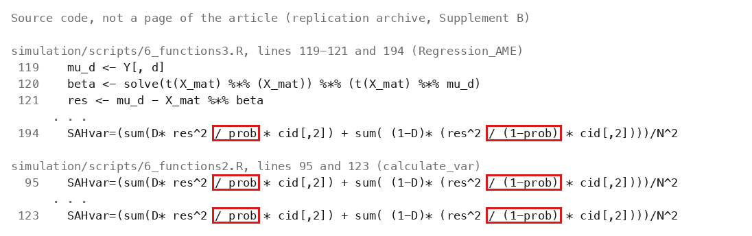
The evidence is an exact counterexample. Let NN be a multiple of 88. Under independent assignment, a quarter of the nodes have propensity 1/21/2 and treated circle averages ai=+1a_i=+1 or −1-1, in equal numbers; the others have propensity 1/101/10 and treated circle average 00. All control circle averages are 00, there is no interference at d=0d=0, and ci(0)=1c_i(0)=1. The covariates are the two group indicators, for which the logistic model holds, and the parameter space is the compact set on which the fitted propensities lie in [1/20,19/20][1/20,19/20]. The AME equals 00 and the coefficients β1,N\beta_{1,N} and β0,N\beta_{0,N} equal 00. Let SS be the sum of aiZia_iZ_i over the first group and p^H\widehat p_H the fitted propensity of that group. Then τ^IPW=S/(Np^H)\widehat\tau_{\mathrm{IPW}}=S/(N\widehat p_H). A direct computation gives τ^IPW−2S/N=Op(N−1)\widehat\tau_{\mathrm{IPW}}-2S/N=O_p(N^{-1}) and NVar⁡(τ^IPW)→1/4N\operatorname{Var}(\widehat\tau_{\mathrm{IPW}})\to1/4. The printed estimator satisfies NV^SAHobs→2/25N\widehat V^{\mathrm{obs}}_{\mathrm{SAH}}\to2/25 in probability, a ratio of 8/258/25 to the variance. For the corrected estimator the limit is 1/21/2. By an exact calculation over the assignment distribution at N=32N=32, the variance of τ^IPW\widehat\tau_{\mathrm{IPW}} is 0.012120.01212, the expectation of the printed estimator is 0.002560.00256, and that of the corrected estimator is 0.012980.01298. At N=64N=64 the three values are 0.004830.00483, 0.001450.00145 and 0.007640.00764. The nominal 95%95\% interval built on the printed estimator has limiting coverage 2Φ(1.968/25)−1≈0.732\Phi(1.96\sqrt{8/25})-1\approx0.73.

What survives

The experimental SAH estimator (20) of the article, which is (24) of Supplement A, uses unweighted residuals with a common pp; it is a different formula and is unaffected. The experimental simulations, the AME, the point estimators and the randomization tests are also unaffected by this error, and the observational HAC display is not touched by this point. The forest application of Section 8.2 reports HAC intervals, not observational SAH intervals; this error does not establish that any reported interval changes. What changes is the SAH display of A.6 and, with it, the intended IPW interval of Proposition 4(i) there. The corrected display removes the double weighting and adds no assumption. The general interval also requires the corrected linearization and fitted values in P004-E001.

Corrected

“where ϵ^i=N1NZip(Oi∣θ^MLE)(μi(Y;d)−Oi′β^1,N)+N0N1−Zi1−p(Oi∣θ^MLE)(μi(Y;d)−Oi′β^0,N)\widehat\epsilon_i=\frac{N_1}{N}\frac{Z_i}{p(\colorbox{#ffe58a}{$O_i$}|\widehat\theta_{\mathrm{MLE}})}\big(\mu_i(\mathbf Y;d)-O_i'\widehat\beta_{1,N}\big)+\frac{N_0}{N}\frac{1-Z_i}{1-p(\colorbox{#ffe58a}{$O_i$}|\widehat\theta_{\mathrm{MLE}})}\big(\mu_i(\mathbf Y;d)-O_i'\widehat\beta_{0,N}\big). … Similarly, we can similarly define a Sävje, Aronow and Hudgens (2018) type variance estimator as in (20):

V^SAHobs(d)=1N12∑i=1NZici(d)ϵ^i2+1N02∑i=1N(1−Zi) ci(d)ϵ^i2,”\widehat V^{\mathrm{obs}}_{\mathrm{SAH}}(d)=\colorbox{#ffe58a}{$\displaystyle \frac1{N_1^2}$}\sum_{i=1}^NZ_ic_i(d)\widehat\epsilon_i^2+\colorbox{#ffe58a}{$\displaystyle \frac1{N_0^2}$}\sum_{i=1}^N(1-Z_i)\,c_i(d)\widehat\epsilon_i^2,\text{''}

where N1=∑i=1NZiN_1=\sum_{i=1}^NZ_i and N0=N−N1N_0=N-N_1, and the entire contribution from an empty arm is set to 00. Equivalently, with the unweighted residuals r^ia=μi(Y;d)−Oi′β^a,N\widehat r_{ia}=\mu_i(\mathbf Y;d)-O_i'\widehat\beta_{a,N} and p^i=p(Oi∣θ^MLE)\widehat p_i=p(O_i|\widehat\theta_{\mathrm{MLE}}),

V^SAHobs(d)=1N2∑i=1Nci(d){Zir^i12p^i 2+(1−Zi)r^i02(1−p^i)2}.\widehat V^{\mathrm{obs}}_{\mathrm{SAH}}(d)=\frac1{N^2}\sum_{i=1}^Nc_i(d)\left\{\frac{Z_i\widehat r_{i1}^2}{\widehat p_i^{\,2}}+\frac{(1-Z_i)\widehat r_{i0}^2}{(1-\widehat p_i)^2}\right\}.

The two forms agree whenever both arms are nonempty. These displays isolate the double weighting. For the corrected Proposition 4 of A.6, use the fitted values f^ia\widehat f_{ia} of P004-E001 in place of Oi′β^a,NO_i'\widehat\beta_{a,N} in the residuals.

Crop of the line that defines epsilon-hat_i as N_1 over N times Z_i over p(O_j | theta-hat_MLE) times a treated residual, plus N_0 over N times (1 minus Z_i) over (1 minus p(O_j | theta-hat_MLE)) times a control residual; the sentence 'The formula is similar to (6), except now that the residuals are weighted with the inverse propensity scores'; and the display of V-hat-obs-SAH(d). Red boxes mark the denominators p squared (O_i | theta-hat_MLE) and (1 minus p(O_i | theta-hat_MLE)) squared of the two sums.
Supplement A, p. 15, the residual ϵ^i\widehat\epsilon_i of A.6 and the observational SAH estimator. The residual in the first line already carries the inverse propensity weights; the two marked denominators divide its square by the squared propensities again.
Bar chart with three groups, N = 32, N = 64 and the limit as N tends to infinity. The vertical axis is the expected variance estimate divided by the true variance, from 0 to 2.3, with a horizontal line at 1 labelled 'true variance'. Orange bars, as printed: 0.21, 0.30 and 0.32, all far below the line. Blue bars, corrected: 1.07, 1.58 and 2.00, all above the line.
The observational SAH estimator, as printed and as corrected, in the example described under Evidence. Each bar is the expected value of the estimator divided by the variance of τ^IPW\widehat\tau_{\mathrm{IPW}}, computed exactly at N=32N=32 and N=64N=64; the third group is the ratio of the limits of NN times each quantity. As printed: 0.210.21, 0.300.30, 0.320.32. Corrected: 1.071.07, 1.581.58, 2.002.00.

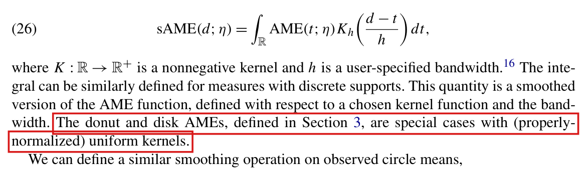
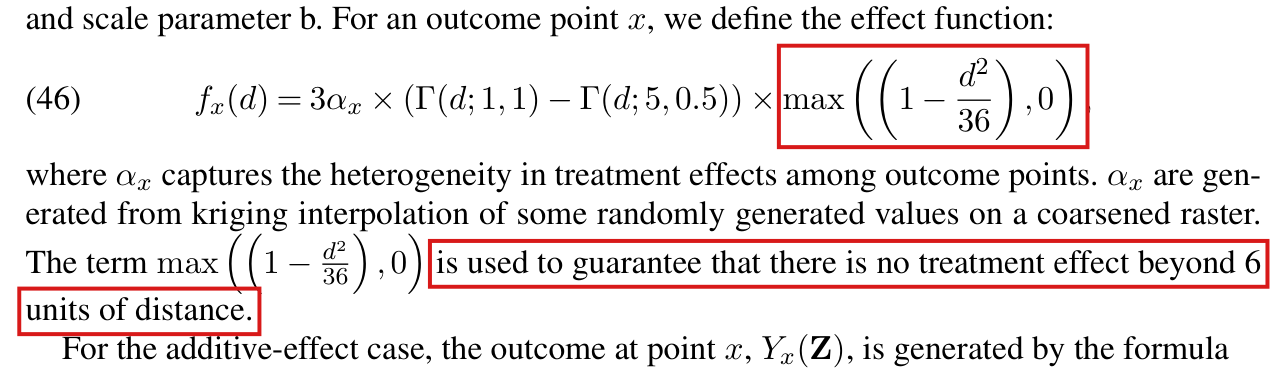
The cutoff h(d)=2dˉ+2dh(d)=2\bar d+2d is sufficient for C3 with point nodes; with polygon nodes adding a uniform bound on the source polygon’s diameter gives a sufficient cutoff, and a lower bound on polygon area does not give C4.

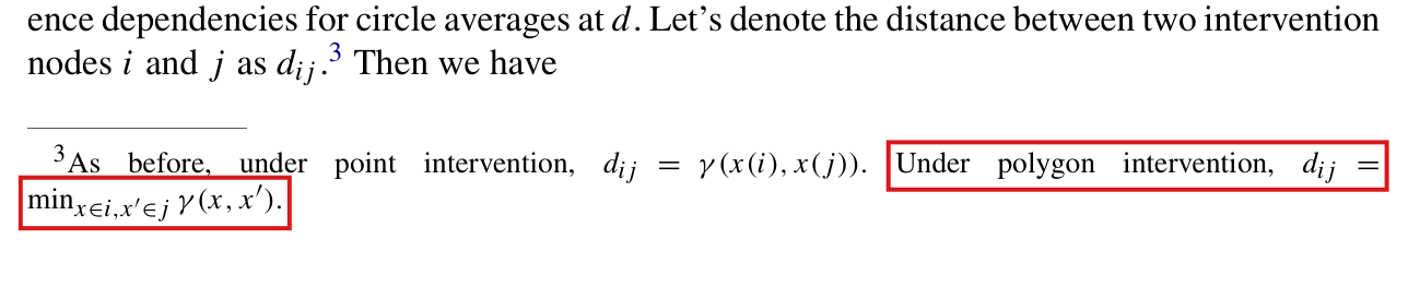
Section 4, p. 752 (PDF p. 9), the paragraph after C3; p. 753 (PDF p. 10), the sentence on polygon interventions after C4; footnote 25, p. 763 (PDF p. 20)

See also under Formal statements (Lean): P004-T16, P004-T17

As printed

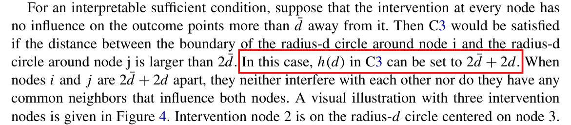
P. 752: “For an interpretable sufficient condition, suppose that the intervention at every node has no influence on the outcome points more than dˉ\bar d away from it. Then C3 would be satisfied if the distance between the boundary of the radius-d circle around node i and the radius-d circle around node j is larger than 2dˉ2\bar d. In this case, h(d)h(d) in C3 can be set to 2dˉ+2d2\bar d+2d.”

P. 753: “For polygon-intervention experiments, one may require that the size of each polygon is larger than a threshold value (thus ensuring adequate spacing between nonadjacent polygons).”

Footnote 25, p. 763: “To be precise, for AME at distance value d, we set the bandwidth at 2d~+2d2\tilde d+2d, as discussed in Section 4.”

The problem

The distance between two polygon nodes is the minimum distance between them (footnote 3). With that distance, a third polygon ℓ\ell can lie within dˉ\bar d of the averaging regions of both ii and jj while ii and jj are farther apart than 2dˉ+2d2\bar d+2d: the point of ℓ\ell nearest to one region and the point of ℓ\ell nearest to the other may be far from each other. The printed rule treats them as one point, which is right for a point node. For polygons a sufficient rule adds a uniform bound on the diameter of the common source polygon. Separately, a lower bound on the area of each polygon does not bound the number of polygons within a fixed distance of a given polygon, because long, thin polygons of fixed area can lie arbitrarily close together. The parenthesis on p. 753 does not give C4. The paper suggests setting the cutoff value d~\tilde d of the spatial HAC variance estimator (19) equal to h(d)h(d) (p. 755, PDF p. 12). With polygon nodes, a cutoff value set by the printed rule can leave out pairs of nodes whose circle averages depend on a common assignment. Footnote 25 applies the cutoff rule to the village polygons of the first application.

Evidence an exact counterexample

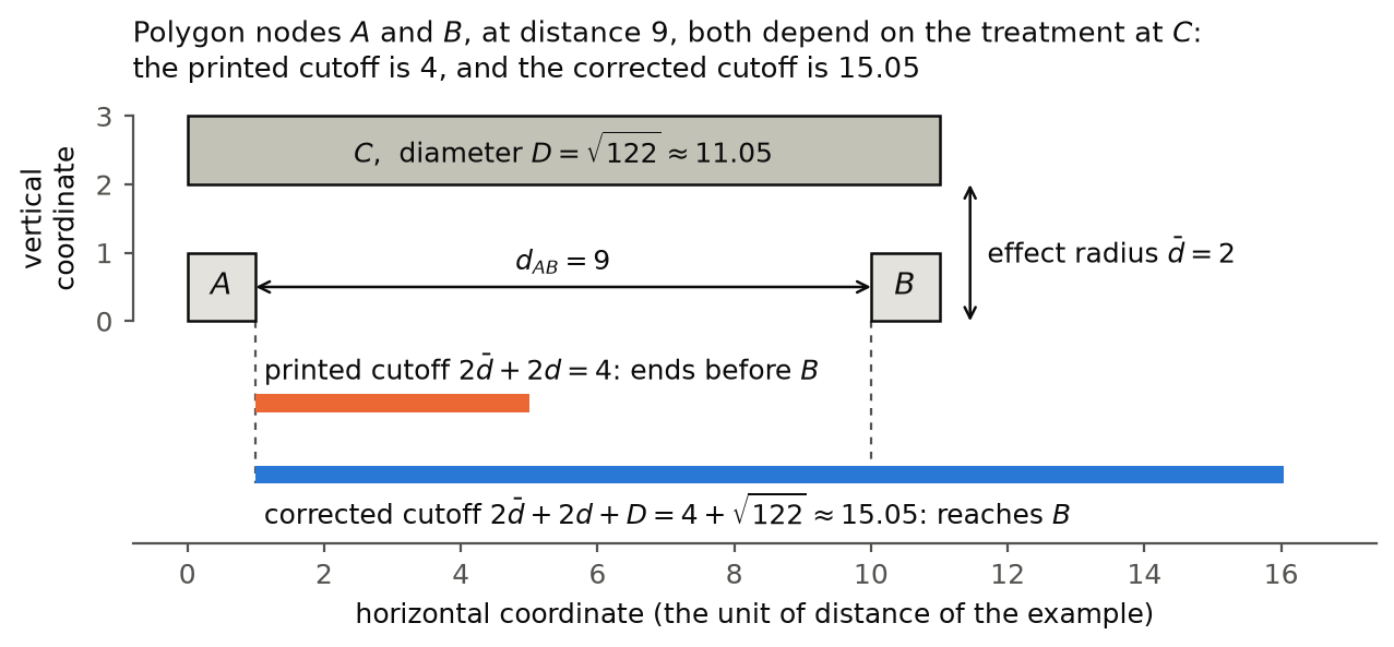
The evidence is two exact counterexamples and a derivation of the corrected bounds. First, let A=[0,1]×[0,1]A=[0,1]\times[0,1], B=[10,11]×[0,1]B=[10,11]\times[0,1] and C=[0,11]×[2,3]C=[0,11]\times[2,3], with independent Bernoulli(1/2)(1/2) assignments, dˉ=2\bar d=2, d=0d=0 and Lebesgue measure. Let Yx(z)=zCY_x(\mathbf z)=z_C for x∈A∪Bx\in A\cup B and Yx(z)=0Y_x(\mathbf z)=0 elsewhere. Every affected point is within distance 22 of CC, and AA and BB affect nothing. The circle averages at AA and BB both equal ZCZ_C. Then sAB(0)=1s_{AB}(0)=1 and their covariance is 1/41/4, while dAB=9>2dˉ+2d=4d_{AB}=9>2\bar d+2d=4. A variant with d=dˉ=1d=\bar d=1 has C=[0,11]×[3,4]C=[0,11]\times[3,4] and unit mass on the outcome points (1/2,2)(1/2,2) and (21/2,2)(21/2,2), where the outcome equals zCz_C. In it dAB=9>4d_{AB}=9>4, the radius-11 contours of AA and BB are 7>2dˉ=27>2\bar d=2 apart, and again sAB(1)=1s_{AB}(1)=1 with covariance 1/41/4.

The figure draws the first example to scale, and the table gives the distances in both examples. In each example the printed cutoff is 44, and AA and BB are 99 apart. The polygon CC has diameter D=112+12=122≈11.05D=\sqrt{11^2+1^2}=\sqrt{122}\approx11.05, which is the largest of the three diameters. With this diameter, I obtain the corrected cutoff 2dˉ+2d+D=4+122≈15.052\bar d+2d+D=4+\sqrt{122}\approx15.05, which is larger than dAB=9d_{AB}=9.

The two counterexamples to the printed cutoff rule.
QuantityFirst exampleSecond example
Distance value dd0011
Effect radius dˉ\bar d2211
Polygon CC[0,11]×[2,3][0,11]\times[2,3][0,11]×[3,4][0,11]\times[3,4]
Printed cutoff 2dˉ+2d2\bar d+2d4444
Distance dABd_{AB}9999
sAB(d)s_{AB}(d)1111
Covariance of the circle averages at AA and BB1/41/41/41/4
Largest diameter DD, that of CC122≈11.05\sqrt{122}\approx11.05122≈11.05\sqrt{122}\approx11.05
Corrected cutoff 2dˉ+2d+D2\bar d+2d+D4+122≈15.054+\sqrt{122}\approx15.054+122≈15.054+\sqrt{122}\approx15.05

Second, for n≥1n\ge1 let P0=[0,1]×[0,1]P_0=[0,1]\times[0,1] and Pk+1=[2,2+n]×[2k/n,(2k+1)/n]P_{k+1}=[2,2+n]\times[2k/n,(2k+1)/n] for 0≤k<n0\le k<n. These n+1n+1 polygons are pairwise disjoint, each has area 11, and each lies within distance less than 22 of P0P_0. Then ∣Sn+1(P0;2)∣=n+1|S_{n+1}(P_0;2)|=n+1, which is unbounded in nn.

For the corrected cutoff, suppose that sij(d)=1s_{ij}(d)=1 through a third node ℓ\ell of diameter at most DD. There exist outcome points xx and yy, both affected by the third node, in the averaging regions of ii and jj, points a∈ia\in i and b∈jb\in j such that ∥a−x∥≤d\|a-x\|\le d and ∥b−y∥≤d\|b-y\|\le d, and points u,v∈ℓu,v\in\ell such that ∥x−u∥≤dˉ\|x-u\|\le\bar d, ∥y−v∥≤dˉ\|y-v\|\le\bar d and ∥u−v∥≤D\|u-v\|\le D. By the triangle inequality along a,x,u,v,y,ba,x,u,v,y,b, I have dij≤2dˉ+2d+Dd_{ij}\le2\bar d+2d+D. If ℓ=i\ell=i or ℓ=j\ell=j, I have dij≤d+dˉd_{ij}\le d+\bar d by the same argument. For the count, suppose every polygon has diameter at most DD, and fix a point qq of polygon ii. If dij≤rd_{ij}\le r, every point of jj is within r+2Dr+2D of qq. The polygons of SN(i;r)S_N(i;r) have disjoint interiors, each has area at least aa, and all lie in the disk of radius r+2Dr+2D about qq. Comparing areas, I obtain a ∣SN(i;r)∣≤π(r+2D)2a\,|S_N(i;r)|\le\pi(r+2D)^2.

What survives

Proposition 1 uses neither C3 nor C4, and Propositions 2–4 assume both directly; these counterexamples do not refute them or the implication from C3 and C4 to C4A. The rule h(d)=2dˉ+2dh(d)=2\bar d+2d stands for point nodes. No simulation result or application interval is shown to change: I did not recompute the application, which reports its intervals for a range of assumed interference radii. What changes is the justification of the cutoff for polygon nodes. For polygons, C3 and C4 are either assumed directly or derived under the additional geometric conditions below.

Corrected

P. 752: “For an interpretable sufficient condition, suppose that the intervention at every node has no influence on the outcome points more than dˉ\bar d away from it. Then, for point interventions, C3 would be satisfied if the distance between the boundary of the radius-d circle around node i and the radius-d circle around node j is larger than 2dˉ2\bar d. In this case, h(d)h(d) in C3 can be set to 2dˉ+2d2\bar d+2d. For polygon interventions, if every polygon has diameter at most D<∞D<\infty, uniformly in the sample size, h(d)h(d) in C3 can be set to 2dˉ+2d+D2\bar d+2d+D.”

Stated in full, the cutoff rule for polygon interventions is as follows. Let dijd_{ij} be the minimum distance between the points of node ii and the points of node jj, as in footnote 3, and let the diameter of a node be the largest distance between two of its points. Suppose that the circle average (2) at distance value dd uses only outcome points within distance dd of its node, which holds for the circle, the donut and the disk. Suppose further that the intervention at every node has no influence on the outcome points more than dˉ\bar d away from it, and that every node has diameter at most D<∞D<\infty, where dˉ\bar d and DD do not depend on the sample size. Then for all nodes i≠ji\ne j,

sij(d)=1impliesdij≤2dˉ+2d+D,s_{ij}(d)=1\quad\text{implies}\quad d_{ij}\le2\bar d+2d+\colorbox{#ffe58a}{$\displaystyle D$},

and C3 holds with h(d)=2dˉ+2d+Dh(d)=2\bar d+2d+\colorbox{#ffe58a}{$D$}. For point interventions every node has diameter 00, and the rule is the printed h(d)=2dˉ+2dh(d)=2\bar d+2d.

P. 753: “For polygon-intervention experiments, a lower bound on the area of each polygon does not ensure C4. In the Euclidean plane, if the polygons have pairwise disjoint interiors, area at least a>0a>0 and diameter at most D<∞D<\infty, uniformly in the sample size, then ∣SN(i;r)∣≤π(r+2D)2/a|S_N(i;r)|\le\pi(r+2D)^2/a for all ii and all r≥0r\ge0, and C4 holds with b(r)=π(r+2D)2/ab(r)=\pi(r+2D)^2/a.”

Footnote 25: “To be precise, for AME at distance value d, we set the bandwidth at 2d~+2d2\tilde d+2d, the rule of Section 4 for point interventions. For village polygons this bandwidth is a sensitivity choice; the premise of a local effect radius does not establish that it is sufficient.”

Alternatively, C3 and C4 may be assumed directly for polygon interventions, without the claim that a local effect radius and a lower bound on area establish them.

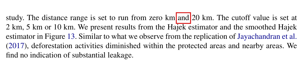
Crop of seven lines of the paragraph that begins 'For an interpretable sufficient condition'. A red box marks the sentence 'In this case, h(d) in C3 can be set to 2 d-bar + 2d.'
Section 4, p. 752 (PDF p. 9), the paragraph after C3. The marked sentence sets the cutoff of C3 to 2dˉ+2d2\bar d+2d with no restriction to point nodes.
Crop of five lines of text. A red box marks the parenthesis '(thus ensuring adequate spacing between nonadjacent polygons)' in the sentence 'For polygon-intervention experiments, one may require that the size of each polygon is larger than a threshold value'.
Section 4, p. 753 (PDF p. 10), the end of the paragraph after C4. The marked parenthesis says that a lower bound on polygon size ensures adequate spacing.
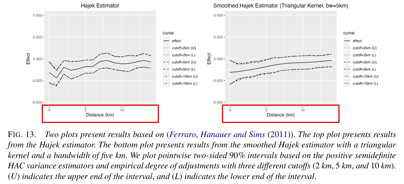
Crop of footnotes 24 and 25. A red box marks '2 d-tilde + 2d' in footnote 25, 'To be precise, for AME at distance value d, we set the bandwidth at 2 d-tilde + 2d, as discussed in Section 4.'
Footnote 25, p. 763 (PDF p. 20). The marked bandwidth applies the cutoff rule of Section 4 to the village polygons of the first application.
Diagram in the plane, drawn to scale, with horizontal coordinates from 0 to 16 and vertical coordinates from 0 to 3. Two unit squares labelled A and B sit on the horizontal axis, A from 0 to 1 and B from 10 to 11. A double arrow between them is labelled 'd AB = 9'. A long grey rectangle labelled 'C, diameter D = square root of 122, about 11.05' lies above them, from 0 to 11 across and from 2 to 3 in height. A vertical double arrow from the lower edge of C to the lower edge of B is labelled 'effect radius d-bar = 2'. Below the squares, two horizontal bars start at the right edge of A. A short orange bar of length 4 is labelled 'printed cutoff 2 d-bar + 2d = 4: ends before B'. A long blue bar of length about 15.05 is labelled 'corrected cutoff 2 d-bar + 2d + D = 4 + square root of 122, about 15.05: reaches B'. Dashed vertical lines mark the right edge of A and the left edge of B. The title reads: 'Polygon nodes A and B, at distance 9, both depend on the treatment at C: the printed cutoff is 4, and the corrected cutoff is 15.05'.
The first counterexample, drawn to scale. The squares A=[0,1]×[0,1]A=[0,1]\times[0,1] and B=[10,11]×[0,1]B=[10,11]\times[0,1] are 99 apart, and the treatment at the polygon C=[0,11]×[2,3]C=[0,11]\times[2,3] sets the outcome on both of them, within the effect radius dˉ=2\bar d=2. Each bar is a cutoff, drawn as a length from AA toward BB. The printed cutoff 2dˉ+2d=42\bar d+2d=4 ends before BB. The corrected cutoff 2dˉ+2d+D=4+122≈15.052\bar d+2d+D=4+\sqrt{122}\approx15.05, where D=122D=\sqrt{122} is the diameter of CC, reaches BB.

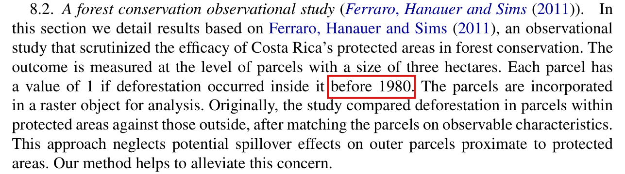
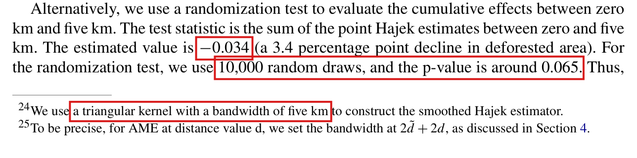
The statistic −0.034-0.034 is an unweighted sum of six distance-specific Hajek estimates, not a 3.4 percentage point decline in deforested area, and its sign does not by itself show a net gain over the area.

Section 8.1, last paragraph of p. 763 (PDF p. 20), continuing on p. 764 (PDF p. 21) after Figure 11

See also under Formal statements (Lean): P004-T5, P004-T6, P004-T37

As printed

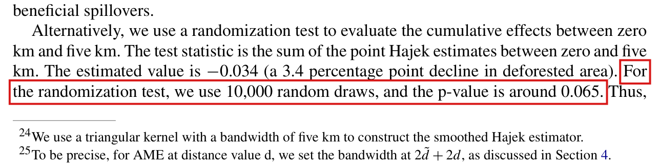
“Alternatively, we use a randomization test to evaluate the cumulative effects between zero km and five km. The test statistic is the sum of the point Hajek estimates between zero and five km. The estimated value is −0.034-0.034 (a 3.4 percentage point decline in deforested area). For the randomization test, we use 10,000 random draws, and the p-value is around 0.065. Thus, we would reject with 90% confidence the sharp null hypothesis. These results indicate that the net gains from the intervention were indeed beneficial, with no indication of substantial leakage.”

The problem

Each Hajek estimate τ^HA(d)\widehat{\tau}_{\mathrm{HA}}(d) of (16) is a difference between treated and control villages in the mean of a circle average (2). In this application it is a difference in the share of deforested pixels at distance dd. The test statistic adds six of these differences, for d=0,1,…,5d=0,1,\dots,5 km, with no weights and no denominator.

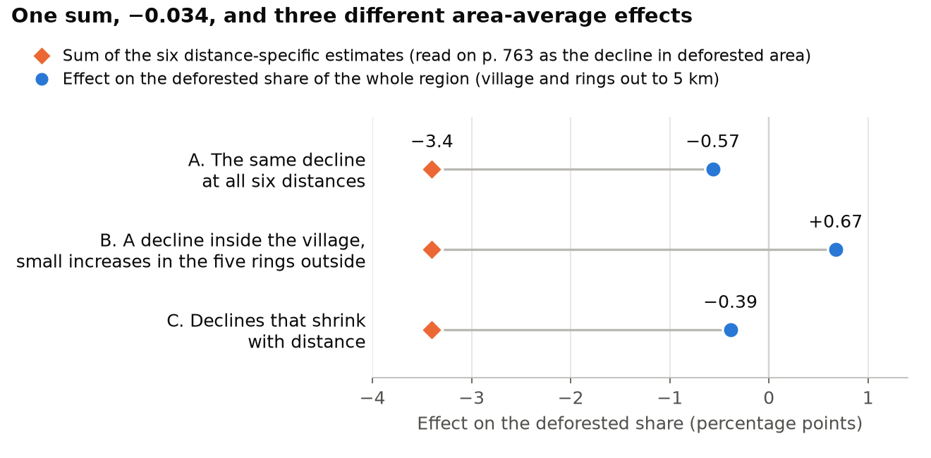
Consider a region made of disjoint distance bins with areas aka_k and effects τk\tau_k, and set A=∑kakA=\sum_k a_k. The effect on the deforested share of the region is the weighted mean ∑k(ak/A)τk\sum_k(a_k/A)\tau_k. Since its weights are nonnegative and sum to one, this mean lies between the smallest and the largest τk\tau_k. In the sum every weight equals one. With equal areas the sum is the mean multiplied by the number of bins. Refining the distance grid can change the sum without changing the effect on the region. The sum therefore does not estimate a change in deforested area, and a negative sum is compatible with an increase in the deforested share of the region. For village polygons, the weights would also depend on the areas of the buffers, on missing pixels and on overlaps.
Evidence an exact counterexample

The evidence is a set of exact examples with binary outcomes. The village is a disc of radius 1 km, with five rings of width 1 km around it. The six areas are proportional to 1,3,5,7,9,111,3,5,7,9,11. The deforested share is 1/101/10 in every bin of a control village. In each of the three examples in the table, the six differences sum to −17/500=−0.034-17/500=-0.034. The effects on the deforested share of the whole region are −0.57-0.57, +0.67+0.67 and −0.39-0.39 percentage points. In the first example, if each ring is split in two, there are eleven bins and the sum is −187/3000≈−0.062-187/3000\approx-0.062, with the same outcomes and the same effect on the region.

Three examples with the published sum. Effects are differences in deforested share, treated minus control.
ExampleEffect in the villageEffects in the five ringsEffect on the region
A−17/3000-17/3000−17/3000-17/3000 in each−17/3000-17/3000
B−2/25-2/25+23/2500+23/2500 in each+121/18000+121/18000
C−1/100-1/100(−9,−6,−5,−3,−1)/1000(-9,-6,-5,-3,-1)/1000−7/1800-7/1800
What survives

The sum remains a valid statistic for the randomization test of the sharp null hypothesis, and its p-value does not depend on how the statistic is described. The estimates and intervals of Figure 11, and the reading that they show no substantial leakage, are unaffected. What is lost is the magnitude of 3.4 points and the statement about net gains so far as it rests on the sum. I have not computed an effect on deforested area for the Uganda data, and the examples say nothing about its sign or size. Whether the replication files give the values −0.034-0.034 and 0.0650.065 is a separate matter (P004-N006).

Corrected

“Alternatively, we use a randomization test to evaluate the cumulative effects between zero km and five km. The test statistic is the sum of the point Hajek estimates between zero and five km. The sum of the distance-specific estimates is −0.034-0.034; this is a summed contrast rather than an estimate of the area-average change in deforestation. For the randomization test, we use 10,000 random draws, and the p-value is around 0.065. Thus, we would reject with 90% confidence the sharp null hypothesis. The randomization test provides evidence against the sharp null. Together with the displayed point estimates, the results suggest beneficial effects, with no indication of substantial leakage at the examined distances.”

A statement about deforested area needs a spatial aggregate that is defined explicitly and computed from the data with its own weights.

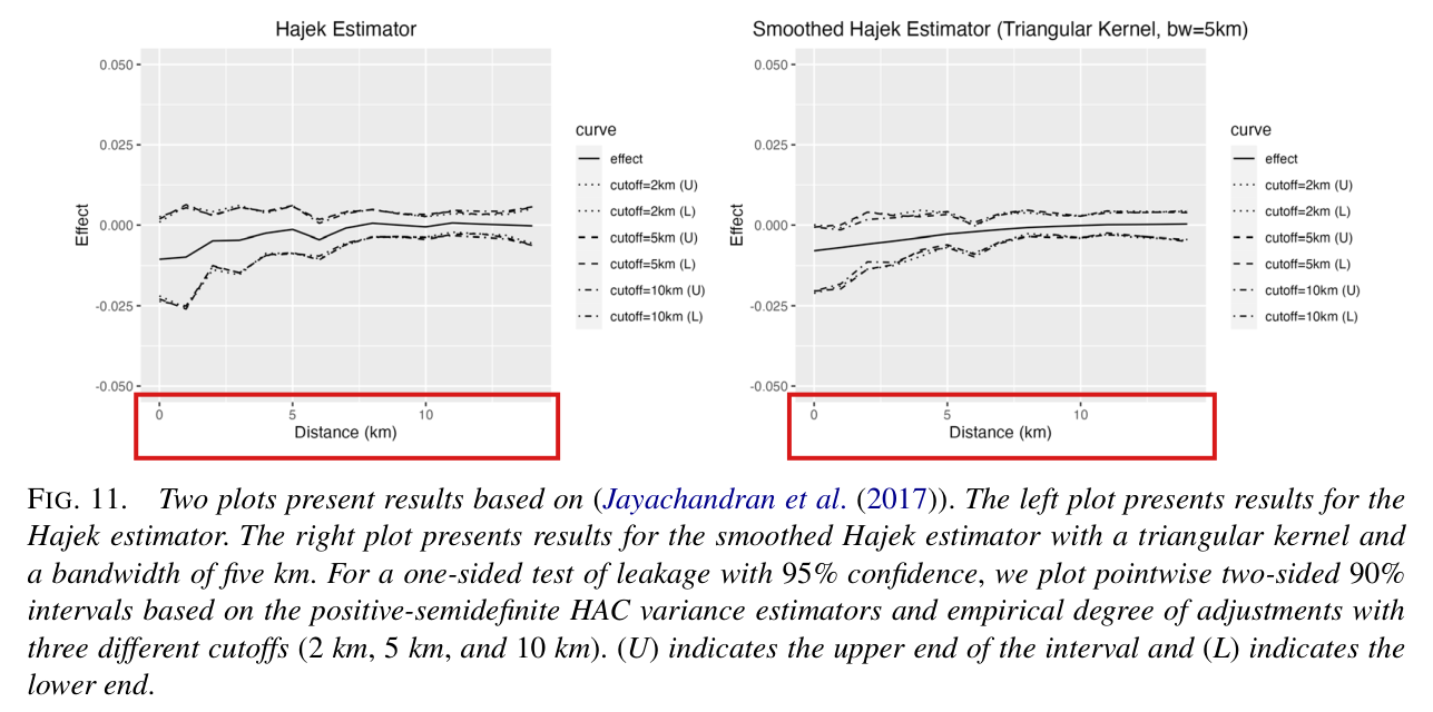
Four lines of body text that define the test statistic as the sum of the point Hajek estimates between zero and five km and give its value, -0.034. A red box marks the parenthesis: (a 3.4 percentage point decline in deforested area).
Section 8.1, last paragraph of p. 763 (PDF p. 20). The marked parenthesis reads the sum of the point estimates as a decline in deforested area.
Three lines of body text. Two red boxes mark the words: These results indicate that the net gains from the intervention were indeed beneficial. The sentence ends: with no indication of substantial leakage.
Continuation of the same paragraph on p. 764 (PDF p. 21), below Figure 11. The marked clause draws a net gain from the test.
Dot plot with three rows, one for each example, on a horizontal axis labelled from -4 to 1 percentage points. In every row an orange diamond sits at -3.4, the sum of the six distance-specific estimates. A blue circle shows the effect on the deforested share of the whole region: -0.57 in example A, +0.67 in example B and -0.39 in example C. A grey line joins the two marks in each row, and a vertical line marks zero.
The three examples of the table. In each, the sum of the six distance-specific estimates is −0.034-0.034, which p. 763 reads as a decline of 3.4 percentage points; the effect on the deforested share of the whole region is −0.57-0.57, +0.67+0.67 or −0.39-0.39 percentage points.

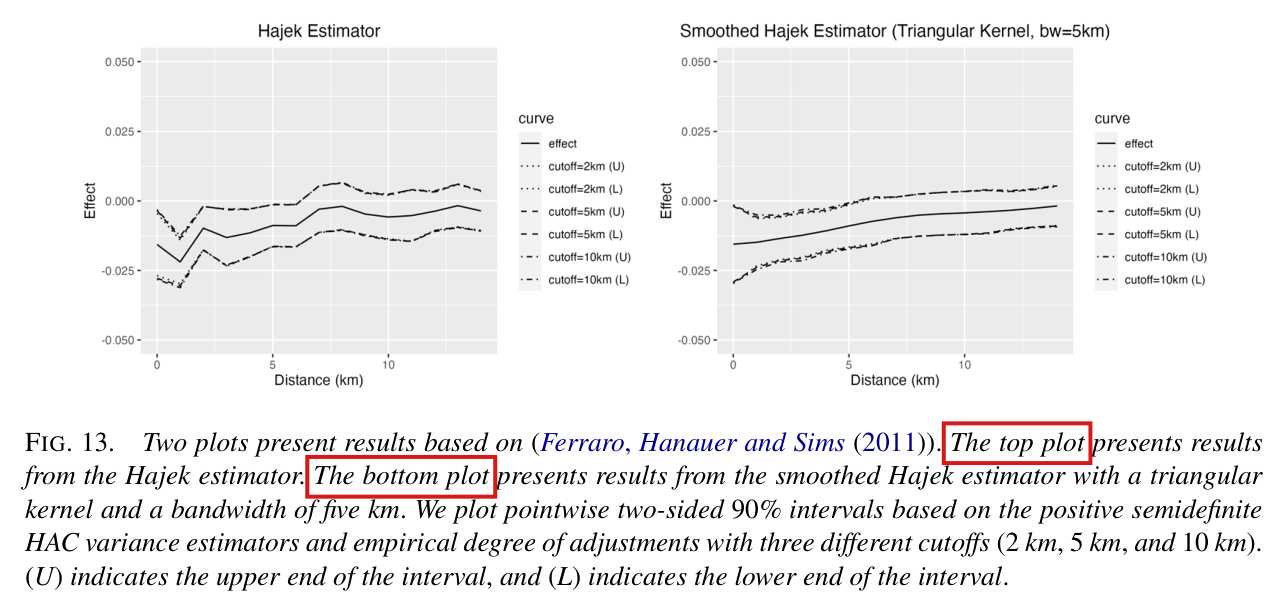
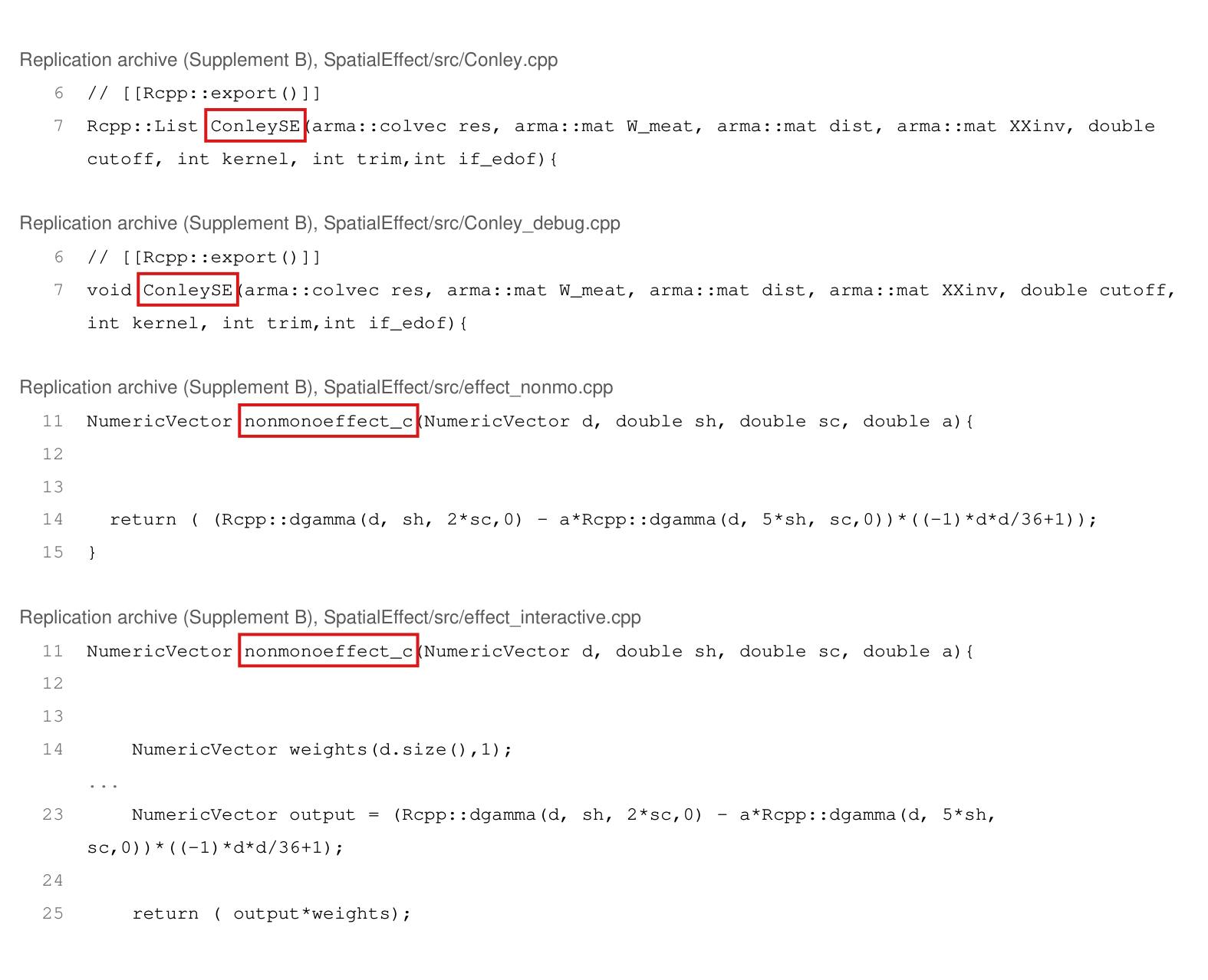
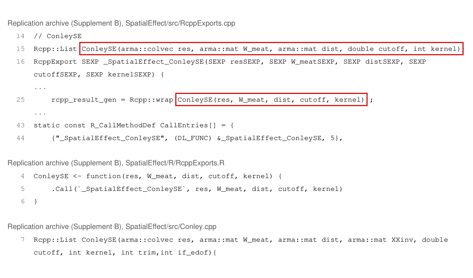
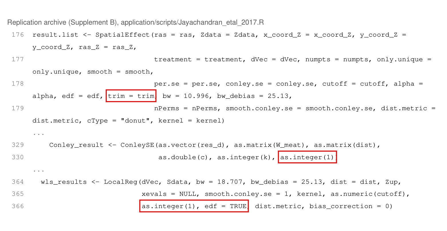
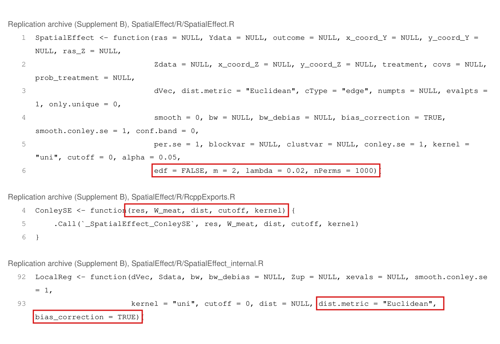
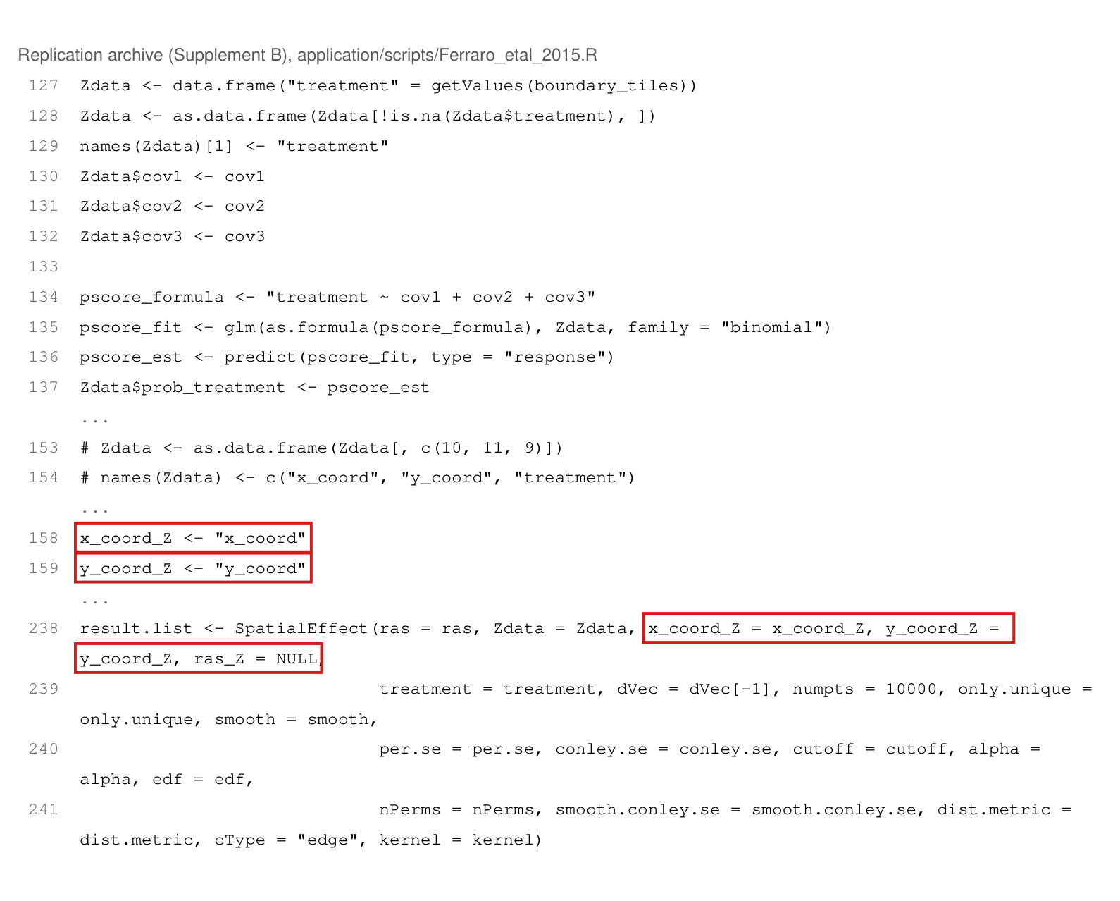
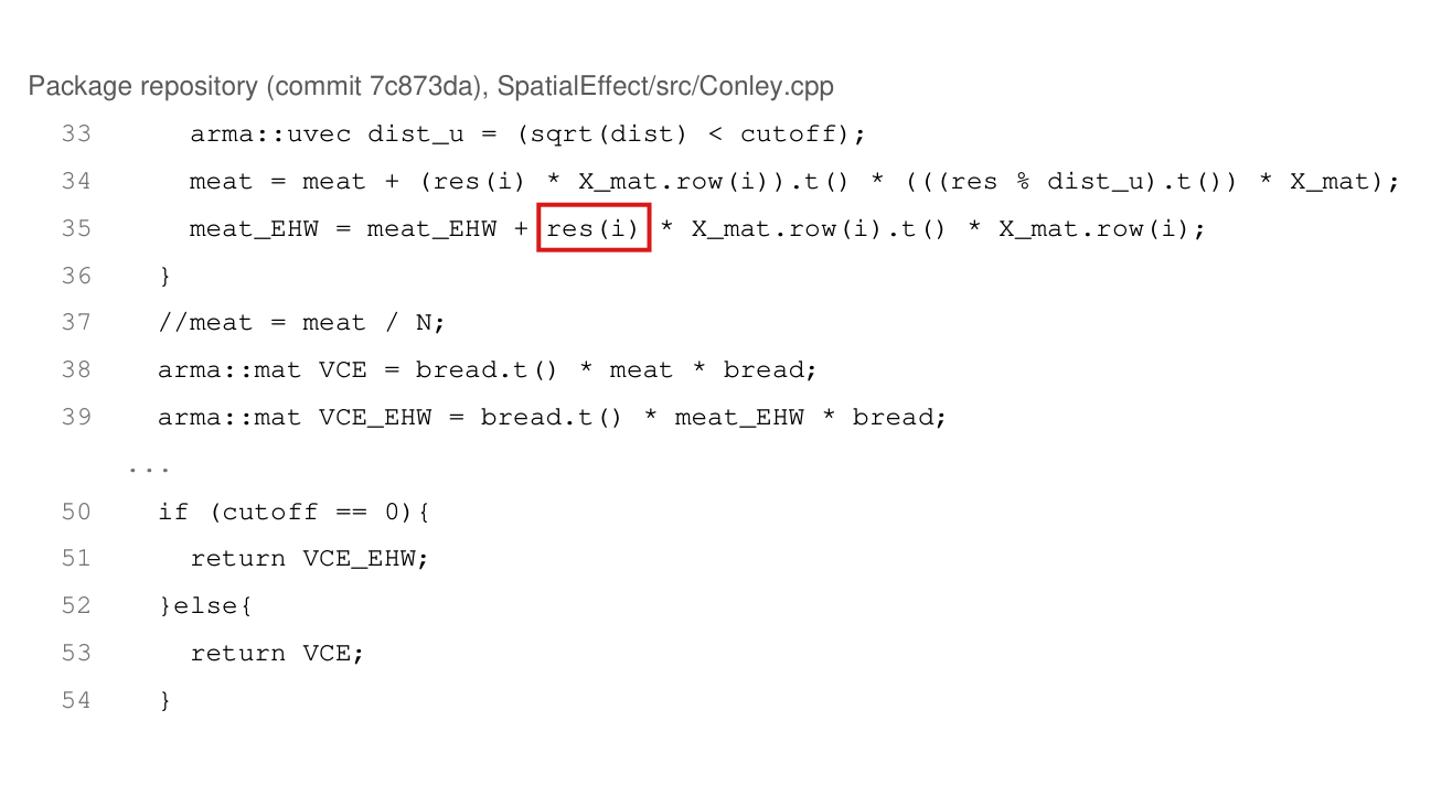
The Costa Rica script in the replication archive fits the propensity scores but omits the argument that activates probability weighting, so, if estimation is reached, its three calls compute an unweighted unsmoothed contrast, with variances that ignore the scores; each call should set prob_treatment = "prob_treatment".

Section 8.2, last paragraph of p. 764 (PDF p. 21), continuing on p. 765, and Figure 13; replication archive (Supplement B), application/scripts/Ferraro_etal_2015.R, lines 134–137, 161 and 238–249, and SpatialEffect/R/SpatialEffect.R, lines 2 and 51–55

As printed

Section 8.2, p. 764: “We estimate the probability for each node to be treated by running a logistic regression model of the treatment indicator on the three covariates used by Ferraro et al., aggregated to the level of intervention nodes: soil quality, distance to the nearest road, and distance to the nearest large city.” And, at the end of p. 764, continuing on p. 765: “We use the same inferential approach as with the Jayachandran et al. study.”

Ferraro_etal_2015.R, line 161 and the first call, lines 238–241:

prob_treatment <- "prob_treatment"

result.list <- SpatialEffect(ras = ras, Zdata = Zdata, x_coord_Z = x_coord_Z, y_coord_Z = y_coord_Z, ras_Z = NULL, treatment = treatment, dVec = dVec[-1], numpts = 10000, only.unique = only.unique, smooth = smooth, per.se = per.se, conley.se = conley.se, cutoff = cutoff, alpha = alpha, edf = edf, nPerms = nPerms, smooth.conley.se = smooth.conley.se, dist.metric = dist.metric, cType = "edge", kernel = kernel)

SpatialEffect.R, lines 51–55 (the highlighted unit weights are selected by these calls):

if (is.null(prob_treatment)){

pweight <- rep(1, nz)

}else{

pweight <- Zup / Zdata[, "prob_treatment"] + (1 - Zup) / (1 - Zdata[, "prob_treatment"])

}

The problem

Section 8.2 presents the Costa Rica analysis as an instance of the observational extension of Section 6.4, in which estimated treatment probabilities weight the estimator. The script fits the logistic model, stores the fitted probabilities in the table of nodes (lines 134–137), and assigns the name of that column to a variable (line 161). None of its three calls to SpatialEffect (lines 238–249) passes the argument prob_treatment. In R an omitted argument takes its default, here NULL, whatever variable of that name exists in the calling script. With NULL, the function sets every weight to one (lines 51–55).

At a fixed distance, let yiy_i be the circle average of node ii, ziz_i its treatment and pip_i its fitted probability, with all circle averages observed, both treatment groups nonempty and 0<pi<10<p_i<1. If estimation is reached, the calls as written give the unsmoothed contrast

∑iziyi∑izi−∑i(1−zi)yi∑i(1−zi),\frac{\sum_i z_iy_i}{\sum_i z_i}-\frac{\sum_i(1-z_i)y_i}{\sum_i(1-z_i)},

and with the argument supplied the function returns the normalized weighted contrast

∑iziyi/pi∑izi/pi−∑i(1−zi)yi/(1−pi)∑i(1−zi)/(1−pi).\frac{\sum_i z_iy_i/p_i}{\sum_i z_i/p_i}-\frac{\sum_i(1-z_i)y_i/(1-p_i)}{\sum_i(1-z_i)/(1-p_i)}.

The HAC and smoothing code receive the same probability weights, and they too ignore the scores in the calls as written. The released code does not carry out the propensity-adjusted analysis that the text describes. I have not established that these calls produced Figure 13.

Evidence an exact counterexample

I checked the original point-estimation code on small examples with synthetic geometry and verified the contrasts by exact arithmetic. With four nodes, (zi,yi,pi)=(1,0,1/4)(z_i,y_i,p_i)=(1,0,1/4), (1,1,3/4)(1,1,3/4), (0,0,1/4)(0,0,1/4) and (0,0,3/4)(0,0,3/4), each of the three calls gives 1/21/2 as written and 1/41/4 with the argument; the R-level variance calculation with a supplied identity covariance kernel gives 1/81/8 as written and 9/1289/128 with the argument. The other two examples in the table use scores that are the exact maximum likelihood fit of a logistic model on three covariates. These checks did not execute the compiled covariance routine or the complete Costa Rica analysis, and no saved result for that application was available for comparison.

Exact contrasts in three examples.
ExampleCalls as writtenWith prob_treatment supplied
Four nodes1/21/21/41/4
Sixteen nodes, fitted logistic scores1/61/61/121/12
Eight nodes, fitted logistic scores1/21/200
What survives

This omission does not invalidate the logistic fit or the density of the scores in Figure 12. The theory, the simulations and the Uganda application do not depend on these calls. This code defect does not show any value in Figure 13 or any conclusion about leakage to be wrong, since it is not known whether the published figure was computed with or without the weights. Supplying the argument activates the weighted contrast and the weighted smoothing and HAC paths that the function already has. It does not make the variance account for the estimation of the scores, which is a separate matter (P004-E001).

Corrected

In each of the three calls (lines 238, 243 and 248):

result.list <- SpatialEffect(prob_treatment = "prob_treatment", ras = ras, Zdata = Zdata, ...)

Check that the rows of the probabilities, the treatment indicator, the node geometry and the circle averages are aligned, and compute the application again.

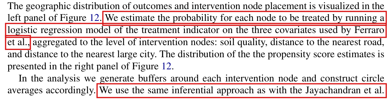
Eight lines of body text. Red boxes mark the beginning of the probability-fitting sentence, through Ferraro et al., and the inferential-approach sentence through Jayachandran et al.; its final word, study, is on the next page.
Section 8.2, end of p. 764 (PDF p. 21). The marked passages describe the fitted treatment probabilities and say that inference follows the approach of the first application; the latter sentence continues on p. 765.

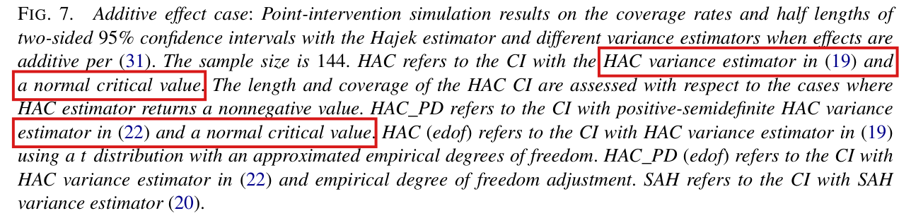
The curves labelled HAC and HAC_PD in Figures 7 and 8 use the variances of (19) and (22), each divided by its own factor μ\mu from Appendix A.7; they differ from the “edof” curves only in the critical value, and the remarks on the length of the intervals hold for these rescaled variances.

Caption of Figure 7 and the labels inherited by Figure 8, p. 761 (PDF p. 18); captions of Figures 2, 3, 5, 6, 8 and 9 of Supplement A (pp. 19–23); the two observations drawn from these figures, p. 756 and p. 761

As printed

Caption of Figure 7, p. 761. HAC refers to the CI with the HAC variance estimator in (19) and a normal critical value. The length and coverage of the HAC CI are assessed with respect to the cases where HAC estimator returns a nonnegative value. HAC_PD refers to the CI with positive-semidefinite HAC variance estimator in (22) and a normal critical value. HAC (edof) refers to the CI with HAC variance estimator in (19) using a tt distribution with an approximated empirical degrees of freedom. HAC_PD (edof) refers to the CI with HAC variance estimator in (22) and empirical degree of freedom adjustment.

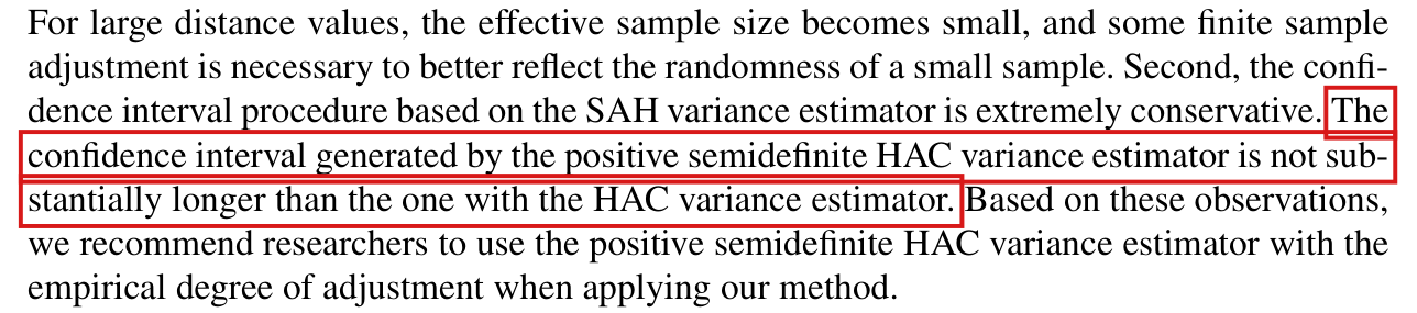
Main text, p. 761. The confidence interval generated by the positive semidefinite HAC variance estimator is not substantially longer than the one with the HAC variance estimator.

Main text, p. 756. We find the HAC-PD estimator returns nonnegative variance estimates with little loss in efficiency.

The problem

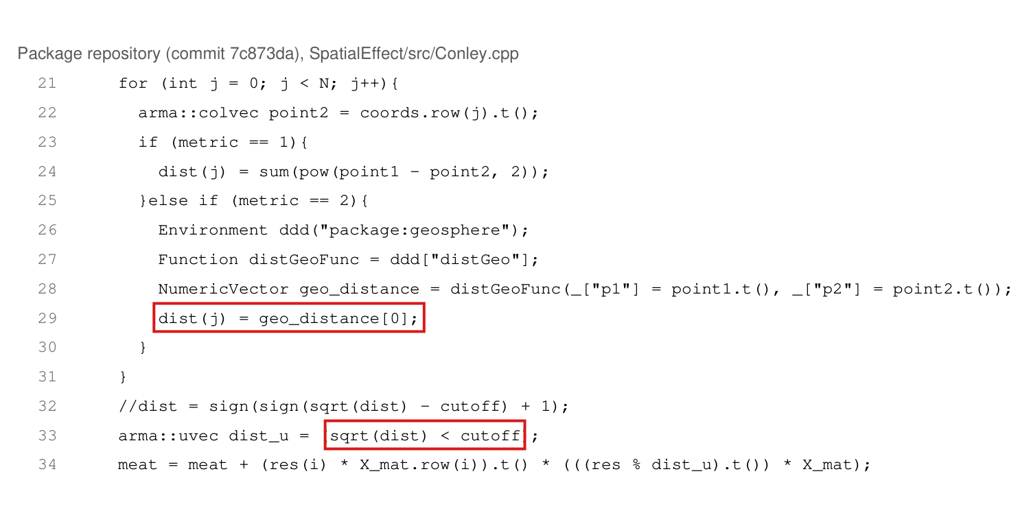
Equations (19) and (22) define the two variance estimators without any rescaling. Appendix A.7 introduces a separate adjustment with two parts: the variance is divided by the factor μ\mu of (44), and the normal critical value is replaced by a quantile of a tt distribution. According to the captions, the curves HAC and HAC_PD use the variances of (19) and (22) with the critical value 1.96, and the curves marked “(edof)” carry the adjustment. The simulation code in the replication files computes something else. The function that returns the variances divides each of them by its own factor and returns V^HAC/μHAC\widehat V_{HAC}/\mu_{HAC} and V^PD/μPD\widehat V_{PD}/\mu_{PD}. The simulation stores these two numbers, and the plotting code uses them for all four curves, with 1.96 for the curves HAC and HAC_PD, which I call the plain curves, and a tt quantile for the “(edof)” curves.

There are three consequences. The figures do not show how the intervals built on (19) and (22) behave without the adjustment. The difference between a plain curve and its “(edof)” curve shows the effect of the critical value only, not of the whole adjustment of A.7. Finally, the remarks that the positive semidefinite interval is “not substantially longer” (p. 761) and comes with “little loss in efficiency” (p. 756) compare two variances that are each divided by a different factor. Since

V^PD/μPDV^HAC/μHAC=V^PDV^HAC⋅μHACμPD,\frac{\widehat V_{PD}/\mu_{PD}}{\widehat V_{HAC}/\mu_{HAC}}=\frac{\widehat V_{PD}}{\widehat V_{HAC}}\cdot\frac{\mu_{HAC}}{\mu_{PD}},

this is not the comparison of (22) with (19).

Evidence an exact counterexample

The evidence is a check of the replication code and two exact examples, computed in rational arithmetic and also run through the published R and C++ routines, which return the same numbers.

The code. In 6_functions3.R (line 196), the function Regression_AME returns a vector whose first two entries are Conley_var2/mu2 and Conley_var2_pd/mu2_pd. In 5_functions_run_simulations.R (lines 264 and 279), it is called with if_edof=1, and these two entries are stored as the HAC and HAC_PD variances. In 5_functions_generate_figures.R (lines 71–99), the square root std1 of the stored HAC variance is computed once. The coverage of the plain HAC curve is the share of draws with abs(tau_est-tau) <= std1 * 1.96, and that of the “(edof)” curve is the share with abs(tau_est-tau) <= std1 * qt(0.975,edof). The HAC_PD curves are computed in the same way from std2.

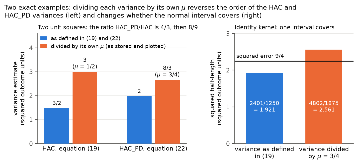
First example. The eight nodes are at (0,0),(2,0),…,(14,0)(0,0),(2,0),\dots,(14,0), and the kernel is uniform with cutoff 1. Then the kernel matrix and its positive semidefinite part are both the identity. Let Z=(0,0,0,0,1,1,1,1)Z=(0,0,0,0,1,1,1,1) and Y=(1,−1,1,−1,5/2,1/2,5/2,1/2)Y=(1,-1,1,-1,5/2,1/2,5/2,1/2). The estimate is 3/23/2, the variance of (19) is 1/21/2, the factor is μ=3/4\mu=3/4, and the stored variance, that is, the variance divided by this factor, is 2/32/3. Suppose that the true value is 0, so that the squared error is 9/49/4. With the critical value 1.96=49/251.96=49/25, the squared half-length of the interval is

(4925)2⋅12=24011250<94with the variance of (19),(4925)2⋅23=48021875>94with the stored variance.\begin{aligned} \Bigl(\frac{49}{25}\Bigr)^2\cdot\frac12&=\frac{2401}{1250}<\frac94&&\text{with the variance of (19)},\\ \Bigl(\frac{49}{25}\Bigr)^2\cdot\frac23&=\frac{4802}{1875}>\frac94&&\text{with the stored variance}. \end{aligned}

The interval of the caption does not cover the true value, and the interval that is plotted does.

Second example. The eight nodes are the corners of two unit squares, and the cutoff is 1. In this order, the nodes are (0,0)(0,0), (1,0)(1,0), (1,1)(1,1), (0,1)(0,1) and (10,0)(10,0), (11,0)(11,0), (11,1)(11,1), (10,1)(10,1). Let

Z=(0,0,1,1,0,0,1,1),Y=(3,−3,1,−1,3,−3,1,−1).Z=(0,0,1,1,0,0,1,1),\qquad Y=(3,-3,1,-1,3,-3,1,-1).
Second example: the variances as defined and as stored by the simulation code.
HAC, (19)HAC_PD, (22)
Variance as defined3/23/222
Factor μ\mu1/21/23/43/4
Variance divided by μ\mu, as stored338/38/3

The ratio of the HAC_PD variance to the HAC variance is 4/34/3 as defined and 8/98/9 as stored. The order of the two variances is reversed.

Direction for the uniform kernel. For the uniform kernel the factor satisfies 0≤μ<10\le\mu<1. On the draws where μ>0\mu>0 and the variance of (19) is nonnegative, the plotted normal interval contains the interval built on (19), and the coverage of the latter cannot exceed that of the plotted curve on those draws.

What is not established. The simulation outputs are not in the replication archive, and I did not regenerate the simulations. The size of the differences in Figures 7 and 8 is not known, and I do not claim that the intervals built on (22) are substantially longer than those built on (19) in the designs of the paper. The two examples show what the rescaling can do. They are not reconstructions of the simulations.

What survives

This discrepancy does not refute the estimators (19) and (22), the positive semidefinite construction, the asymptotic results, the figures for the mean squared error or the randomization tests. The plotted curves describe the procedures that were computed, once they are relabelled. The captions of the two applications already name the positive semidefinite estimator with the adjustment; I have not established a change in their numerical results. The recommendation on p. 761 can stand as a statement about the adjusted procedures. What changes is the scope of the two observations: they hold for the rescaled variances, and the figures do not separate the whole adjustment of A.7 from the intervals built on (19) and (22). Whether the positive semidefinite variance may be divided by its factor, and the degrees of freedom used for HAC_PD (edof), are treated in P004-N004 and P004-E026.

Corrected

Caption of Figure 7. HAC refers to the CI with the HAC variance estimator in (19), divided by its factor μ\mu of (44), and a normal critical value. … HAC_PD refers to the CI with positive-semidefinite HAC variance estimator in (22), divided by its own factor μ\mu computed from the positive semidefinite kernel, and a normal critical value. HAC (edof) and HAC_PD (edof) use the same two rescaled variances with the empirical tt critical values computed by the simulation code.

Main text, p. 761. The confidence interval generated by the positive semidefinite HAC variance estimator is not substantially longer than the one with the HAC variance estimator, when each variance is divided by its own factor μ\mu.

Main text, p. 756. We find the HAC-PD estimator returns nonnegative variance estimates with little loss in efficiency, when each variance is divided by its own factor μ\mu.

Alternatively, the definitions of the plain curves can stand as printed if those curves are recomputed from the variances of (19) and (22) without the division by μ\mu; the length and efficiency comparisons would then need to be checked again.

Crop of the nine-line caption of Figure 7. It reads in part: HAC refers to the CI with the HAC variance estimator in (19) and a normal critical value. The length and coverage of the HAC CI are assessed with respect to the cases where HAC estimator returns a nonnegative value. HAC_PD refers to the CI with positive-semidefinite HAC variance estimator in (22) and a normal critical value. HAC (edof) refers to the CI with HAC variance estimator in (19) using a t distribution with an approximated empirical degrees of freedom. Red outlines surround the words HAC variance estimator in (19) and a normal critical value, and the words estimator in (22) and a normal critical value.
Caption of Figure 7, p. 761 (PDF p. 18). The outlines mark the two definitions of the plain curves.
Crop of seven lines of text. The marked sentence reads: The confidence interval generated by the positive semidefinite HAC variance estimator is not substantially longer than the one with the HAC variance estimator. It is followed by: Based on these observations, we recommend researchers to use the positive semidefinite HAC variance estimator with the empirical degree of adjustment when applying our method. Red outlines surround the marked sentence, which runs over three lines.
Main text below Figure 7, p. 761 (PDF p. 18). The outline marks the sentence that compares the lengths of the two intervals.
Crop of equation (44) and two lines of text. Equation (44) defines mu as the trace of N sub 1 N sub 0 over N times M times the Hadamard product of Omega and lambda-prime lambda, times M. The text reads: where the circle denotes the pointwise (Hadamard) matrix product. The estimated variance is inflated by one over mu, becoming w-prime Sigma-hat sub HAC w over mu. We further define the quantity. A red outline surrounds the sentence The estimated variance is inflated by one over mu, becoming w-prime Sigma-hat sub HAC w over mu.
Supplement A, Appendix A.7, p. 17. The outline marks the only place where the division of the variance by μ\mu is described.
Two bar charts under the title: Two exact examples: dividing each variance by its own mu reverses the order of the HAC and HAC_PD variances (left) and changes whether the normal interval covers (right). Left panel, two unit squares: for HAC, equation (19), a blue bar of height 3/2 (as defined) and an orange bar of height 3 (divided by mu = 1/2); for HAC_PD, equation (22), a blue bar of height 2 and an orange bar of height 8/3 (mu = 3/4). The vertical axis is the variance estimate in squared outcome units. Right panel, identity kernel: a blue bar of height 2401/1250 = 1.921 for the variance as defined in (19) and an orange bar of height 4802/1875 = 2.561 for the variance divided by mu = 3/4, with a horizontal line at the squared error 9/4. The vertical axis is the squared half-length of the interval in squared outcome units. Only the orange bar reaches above the line.
The two exact examples. Left: in the second example the HAC_PD variance is larger than the HAC variance as defined (22 against 3/23/2) and smaller after each is divided by its own μ\mu (8/38/3 against 33). Right: in the first example the squared half-length of the normal interval is below the squared error 9/49/4 with the variance of (19) and above it after the division by μ=3/4\mu=3/4.

The simulation code uses μPD2/νPD\mu_{\mathrm{PD}}^2/\nu_{\mathrm{PD}} degrees of freedom for the HAC_PD (edof) interval, half of the 2μ2/ν2\mu^2/\nu stated in Supplement A.7, so the coverage and half-lengths plotted for this interval in Figures 7 and 8 belong to an interval at least as wide as the one described; the code should use 2μPD2/νPD2\mu_{\mathrm{PD}}^2/\nu_{\mathrm{PD}}, and the series should be computed again.

Figure 7 (caption) and Figure 8, p. 761 (PDF p. 18); Supplement A, Section A.7, equation (45) and the sentence after it, p. 17; replication archive (Supplement B), simulation/scripts/6_functions3.R, lines 196 and 312, and simulation/scripts/5_functions_generate_figures.R, lines 78–79, 87 and 97

As printed

Caption of Figure 7, p. 761: “HAC_PD (edof) refers to the CI with HAC variance estimator in (22) and empirical degree of freedom adjustment.”

Supplement A, Section A.7, p. 17:

ν=2∗Trace((N1N0NM(Ω∘(λ′λ))M)(N1N0NM(Ω∘(λ′λ))M)).(45)\nu = 2 * \mathbf{Trace}\left(\left(\frac{N_1N_0}{N}\mathbf{M}\left(\Omega\circ\left(\lambda'\lambda\right)\right)\mathbf{M}\right)\left(\frac{N_1N_0}{N}\mathbf{M}\left(\Omega\circ\left(\lambda'\lambda\right)\right)\mathbf{M}\right)\right). \tag{45}

“We use the α2\frac{\alpha}{2}-quantile and (1−α2)\left(1-\frac{\alpha}{2}\right)-quantile of the t-distribution with 2μ2v\frac{2\mu^2}{v} degree of freedom to construct the confidence interval.”

6_functions3.R, line 196 (line 312 is identical), shown here on two lines:

return(c(Conley_var2/mu2,Conley_var2_pd/mu2_pd,SAHvar,\texttt{return(c(Conley\_var2/mu2,Conley\_var2\_pd/mu2\_pd,SAHvar,}

edof=2*mu2^2/v2,edof_pd=mu2_pd^2/v2_pd))\texttt{edof=2*mu2\textasciicircum 2/v2,edof\_pd=}\colorbox{#ffe58a}{$\texttt{mu2\_pd\textasciicircum 2}$}\texttt{/v2\_pd))}

5_functions_generate_figures.R, lines 78–79:

edof[which(edof<=1)]=1

edof_pd[which(edof_pd<=1)]=1

The problem

Supplement A.7 chooses the degrees of freedom by matching two moments. Suppose that a quadratic form has mean μ\mu and variance ν\nu. Divided by μ\mu, it has mean 11 and variance ν/μ2\nu/\mu^2. A chi-square variable with ff degrees of freedom, divided by ff, has mean 11 and variance 2/f2/f. Equating the two variances, I obtain f=2μ2/νf=2\mu^2/\nu, where ν\nu is twice the trace of the squared matrix, as in (45). The caption of Figure 7 applies this adjustment to the HAC interval and to the HAC_PD interval alike.

The two simulation routines, Regression_AME and Regression_AME_obs, return 2μ2/ν2\mu^2/\nu for the HAC estimator and μPD2/νPD\mu_{\mathrm{PD}}^2/\nu_{\mathrm{PD}} for the positive semidefinite one. One C++ routine computes μ\mu and ν\nu for both kernels, and its ν\nu already contains the factor 2 of (45). The value returned for HAC_PD is half of the stated one. The figure code takes this value as the degrees of freedom of the tt quantile, in the coverage and in the median half-length of the HAC_PD (edof) series. Since the positive upper tt critical value decreases as the degrees of freedom grow, the plotted interval is at least as wide as the interval that A.7 describes, and its coverage is at least as high.

The figure code also resets any degrees of freedom below one to one, a rule that A.7 does not state. Let bi≥0b_i\ge 0 be the eigenvalues of the matrix in (45) for a positive semidefinite kernel, not all zero. Then the stated value is (∑ibi)2/∑ibi2≥1(\sum_i b_i)^2/\sum_i b_i^2\ge 1, which implies that the reset has no effect on HAC_PD once the factor is restored. With the factor missing, the reset raises a coded value below one back to one, and it then hides part of the error.

The affected series are HAC_PD (edof) in Figures 7 and 8 and in Figures 2, 3, 5, 6, 8 and 9 of Supplement A. These series are the simulation evidence for the interval that Section 7 recommends. The replication archive does not contain the simulation results needed to recompute these series, and I have not computed the series again.

Evidence an exact counterexample

The evidence is an exact example, computed in rational arithmetic and reproduced by running the unchanged R and C++ routines in the archive. I take six nodes at 0,10,…,500,10,\dots,50 on a line, with Z=(0,0,0,1,1,1)Z=(0,0,0,1,1,1), observed circle averages Y=(0,0,3,1,1,1)Y=(0,0,3,1,1,1) and a kernel cutoff of 11. Since the kernel matrix is the identity, the HAC and HAC_PD estimators coincide. Here λ=(−1,−1,−1,1,1,1)/3\lambda=(-1,-1,-1,1,1,1)/3, and the matrix in (45) is M/6\mathbf{M}/6, where M\mathbf{M} is a projection of rank 44. A direct computation gives μ=2/3\mu=2/3 and ν=2/9\nu=2/9. By A.7, I have 2μ2/ν=42\mu^2/\nu=4 for both estimators. The routines return 44 for HAC and 22 for HAC_PD. The estimate is 00, and both adjusted standard errors equal 11. The half-length of the 95% interval is 2.7762.776 with 44 degrees of freedom and 4.3034.303 with 22. The coded interval contains the value 33, and the stated interval does not.

The table adds two examples. In the second, the kernel is positive semidefinite with two clusters of three nodes, and the reset in the figure code restores the stated value. The third comes from a separate check with eight nodes, where the half-lengths are 2.2342.234 as stated and 2.9052.905 as coded.

The C++ routine stores MA\mathbf{M}A where A.7 has MAM\mathbf{M}A\mathbf{M}, with AA the kernel-weighted matrix. Since M2=M\mathbf{M}^2=\mathbf{M}, the two matrices have the same trace, and their squares have the same trace. The routine computes the μ\mu and ν\nu of A.7, and no other normalization accounts for the missing factor.

Degrees of freedom in three exact examples: the value 2μ2/ν2\mu^2/\nu of A.7, the values returned by the simulation routines, and the value used in the figure code. In each example the HAC and HAC_PD kernels are equal.
Exampleμ\muν\nuA.7HAC, codeHAC_PD, codeHAC_PD, plotted
Six nodes, identity kernel2/32/32/92/944442222
Six nodes, two clusters4/94/932/8132/8111111/21/211
Eight nodes, identity kernel3/43/43/163/1666663333
What survives

No formula in the paper changes. The moment-matching formula in A.7 is correct, and the HAC return expression already uses 2μ2/ν2\mu^2/\nu. Restoring the factor changes no variance estimate, and so it changes no series computed with a normal critical value and no SAH series. The point estimators, the asymptotic results, the mean squared errors and the randomization test do not involve the degrees of freedom. The application scripts compute their intervals by a separate path (P004-N007). What changes is the HAC_PD (edof) series: with the stated degrees of freedom its intervals are no wider, and its coverage no higher, than plotted. The size of the change is not known, and nothing here shows that the recommendation of Section 7 fails.

Corrected

In both return statements of 6_functions3.R (lines 196 and 312):

edof_pd=2*mu2_pd^2/v2_pd\texttt{edof\_pd=}\colorbox{#ffe58a}{$\texttt{2*}$}\texttt{mu2\_pd\textasciicircum 2/v2\_pd}

Then compute again the coverage and the half-length of the HAC_PD (edof) series in Figures 7 and 8 and in Figures 2, 3, 5, 6, 8 and 9 of Supplement A. In 5_functions_generate_figures.R, remove the reset of degrees of freedom below one (lines 78–79), or state the rule in A.7 if it is kept for the HAC series. After the factor is restored, the reset has no effect on HAC_PD whenever the quadratic form is nonzero. The effect of the correction on the published figures remains to be computed.

Five lines from the italic caption of Figure 7. Red boxes mark the sentence: HAC_PD (edof) refers to the CI with HAC variance estimator in (22) and empirical degree of freedom adjustment.
Caption of Figure 7, p. 761 (PDF p. 18). The marked sentence defines the HAC_PD (edof) series as the interval with the positive semidefinite HAC variance estimator (22) and the degrees-of-freedom adjustment of Supplement A.7.
Equation (45): nu equals 2 times the trace of the square of the matrix (N1 N0 / N) M (Omega circ lambda-prime lambda) M, with a red box around the factor 2 and the star after it. Below it, the sentence: We use the alpha/2-quantile and (1 - alpha/2)-quantile of the t-distribution with 2 mu squared over v degree of freedom to construct the confidence interval. A red box marks the fraction 2 mu squared over v.
Supplement A, Section A.7, p. 17: equation (45) and the sentence after it. The marks show the factor 2 in ν\nu and the stated degrees of freedom 2μ2/v2\mu^2/v; the vv of that sentence is the ν\nu of (45).

The recommended interval divides the positive semidefinite HAC variance by a factor μ\mu computed from the trimmed kernel, and this factor can converge to a limit above one; under C1–C5 the adjusted variance can then stay below the variance of the estimator, and the interval can cover too rarely; the guarantee of Proposition 4 carries over once the factor is capped at one.

Section 7, p. 761 (PDF p. 18), end of the paragraph between Figures 7 and 8; Section 5, p. 756 (PDF p. 13), equation (22) and footnote 15; Supplement A, Section A.7, equation (44) and the sentence after it, p. 17; replication archive (Supplement B), simulation/scripts/6_functions3.R, line 196

See also under Formal statements (Lean): P004-T7, P004-T8

Revised: see the history of this entry.

As printed

Section 7, p. 761: “Based on these observations, we recommend researchers to use the positive semidefinite HAC variance estimator with the empirical degree of adjustment when applying our method.”

Section 5, p. 756: “Nonetheless, it is possible to design a biased-upward positive definite estimator.” After (22): “In addition, Σ^HACPD(d)≥Σ^HAC(d)\widehat{\Sigma}^{\mathrm{PD}}_{\mathrm{HAC}}(d)\geq\widehat{\Sigma}_{\mathrm{HAC}}(d).”

Supplement A, Section A.7, p. 17: “The estimated variance is inflated by 1μ\frac{1}{\mu}, becoming w′Σ^HACwμ\frac{\mathbf{w}'\widehat{\Sigma}_{\mathrm{HAC}}\mathbf{w}}{\mu}.”

6_functions3.R, line 196, second returned value: Conley_var2_pd/mu2_pd

The problem

Section 5 shows that the positive semidefinite estimator is at least as large as the HAC estimator, and under the conditions of Proposition 4(ii) the unadjusted HAC interval has asymptotic coverage of at least 1−α1-\alpha. The interval with the positive semidefinite variance V^PD\widehat{V}_{\mathrm{PD}} and a normal critical value inherits this guarantee. The recommended interval is a different one. Section A.7 defines the adjustment for the uniform kernel matrix Ω\Omega only. The replication code extends it to the positive semidefinite estimator: it computes μPD\mu_{\mathrm{PD}} and νPD\nu_{\mathrm{PD}} from the trimmed kernel KPDK^{\mathrm{PD}} of Section 5 in place of Ω\Omega, and it returns V^PD/μPD\widehat{V}_{\mathrm{PD}}/\mu_{\mathrm{PD}}.

The diagonal entries of Ω\Omega equal one, and in the examples below μ\mu tends to one. Trimming the negative eigenvalues adds a positive semidefinite matrix to the kernel, which raises its trace. In the examples below, μPD\mu_{\mathrm{PD}} tends to the average diagonal entry of KPDK^{\mathrm{PD}}, which is 6/56/5 in one and 5/45/4 in the other. Dividing by a factor above one does not inflate the variance. It deflates it, and the upward bias of V^PD\widehat{V}_{\mathrm{PD}} need not make up the difference. The ordering V^PD/μPD≥V^HAC/μ\widehat{V}_{\mathrm{PD}}/\mu_{\mathrm{PD}}\ge\widehat{V}_{\mathrm{HAC}}/\mu can then fail, and NV^PD/μPDN\widehat{V}_{\mathrm{PD}}/\mu_{\mathrm{PD}} can converge to a limit below the limit of NVar⁡(τ^HA)N\operatorname{Var}(\widehat{\tau}_{\mathrm{HA}}). In the examples the tt critical value does not compensate, because the degrees of freedom tend to infinity.

The paper states no theorem for the adjusted estimator; this failure does not contradict Proposition 4 or the printed unadjusted inequality. What fails is the recommendation when it is read as a procedure valid under C1–C5. Figures 7 and 8 report this interval, and the captions of Figures 11 and 13 describe the intervals of the two applications in the same terms.

Evidence an exact counterexample

The evidence is a pair of exact examples that satisfy C1–C5, with the limits derived and the finite matrices computed in rational arithmetic.

First example. For each m≥1m\ge 1, the design has N=5mN=5m nodes in mm blocks. Block bb has a centre at (10b,0)(10b,0) and four leaves at (10b±1,0)(10b\pm 1,0) and (10b,±1)(10b,\pm 1). The assignments are independent with probability 1/21/2. The circle averages at d=0d=0 are y=(0,1,1,−1,−1)y=(0,1,1,-1,-1) in every block under every assignment, so that no interference is present and every treatment effect is zero. Conditions C1–C5 hold, and h(0)=6/5h(0)=6/5 is a valid cutoff in C3. With this cutoff the uniform kernel links the centre to each leaf and links no two leaves. In each block the kernel has eigenvalues −1,1,1,1,3-1,1,1,1,3. After the eigenvalue −1-1 is trimmed, the matrix KPDK^{\mathrm{PD}} has diagonal (3/2,9/8,9/8,9/8,9/8)(3/2,9/8,9/8,9/8,9/8) and trace 66.

I write si=2Zi−1s_i=2Z_i-1. Since ∑iyi=0\sum_i y_i=0 in each block, I have τ^HA=2N−1∑isiyi+Op(N−3/2)\widehat{\tau}_{\mathrm{HA}}=2N^{-1}\sum_i s_iy_i+O_p(N^{-3/2}), and hence NVar⁡(τ^HA)→(4/N)∑iyi2=16/5N\operatorname{Var}(\widehat{\tau}_{\mathrm{HA}})\to (4/N)\sum_i y_i^2=16/5. For a kernel QQ made of identical blocks, NV^QN\widehat{V}_Q equals 4/N4/N times the sum over blocks of t′Qtt'Qt, up to a term that tends to zero in probability, where ti=siyit_i=s_iy_i. Using the independence of the signs, I obtain E[t′Qt]=∑iQiiyi2\mathbb{E}[t'Qt]=\sum_i Q_{ii}y_i^2. This sum is 44 for the uniform kernel and 4⋅9/8=9/24\cdot 9/8=9/2 for KPDK^{\mathrm{PD}}. By the law of large numbers, I find that NV^HAC→16/5N\widehat{V}_{\mathrm{HAC}}\to 16/5 and NV^PD→18/5N\widehat{V}_{\mathrm{PD}}\to 18/5. Finally, μQ\mu_Q equals N−1Trace⁡(Q)N^{-1}\operatorname{Trace}(Q) up to a term that tends to zero, which implies that μ→1\mu\to 1 for the uniform kernel and μPD→6/5\mu_{\mathrm{PD}}\to 6/5. Combining these limits, I obtain

N V^PDμPD→18/56/5=3<165,N\,\frac{\widehat{V}_{\mathrm{PD}}}{\mu_{\mathrm{PD}}}\to\frac{18/5}{6/5}=3<\frac{16}{5},

so the adjusted variance converges to 15/1615/16 of the variance of the estimator. The degrees of freedom 2μPD2/νPD2\mu_{\mathrm{PD}}^2/\nu_{\mathrm{PD}} tend to infinity, and the coverage of the nominal 95% interval tends to 2Φ(z0.97515/16)−1=0.94232\Phi(z_{0.975}\sqrt{15/16})-1=0.9423.

Second example. The blocks now have four nodes at the corners of a unit square, (10b,0)(10b,0), (10b+1,0)(10b+1,0), (10b+1,1)(10b+1,1) and (10b,1)(10b,1). I use disk averages with counting measure. Each node ii has outcome 2Zj−12Z_j-1, where jj is its horizontal neighbour; at the reflection of jj across ii, the outcome is 1−2Zi1-2Z_i. The two effects of ZiZ_i are both at distance one from ii and cancel in every disk centred on ii, so every marginal effect is zero. Here the cutoff h(0)=1h(0)=1 equals the range of the dependence. The trimmed kernel has diagonal 5/45/4. Both unadjusted estimators are asymptotically exact, and the adjusted one converges to 4/54/5 of the variance of the estimator.

Limits in the two examples as N→∞N\to\infty. The last column is the limiting coverage of the nominal 95% interval with variance V^PD/μPD\widehat{V}_{\mathrm{PD}}/\mu_{\mathrm{PD}}.
ExampleμPD\mu_{\mathrm{PD}}NVar⁡(τ^HA)N\operatorname{Var}(\widehat{\tau}_{\mathrm{HA}})NV^PDN\widehat{V}_{\mathrm{PD}}NV^PD/μPDN\widehat{V}_{\mathrm{PD}}/\mu_{\mathrm{PD}}RatioCoverage
Five-node blocks, no interference6/56/516/516/518/518/53315/1615/160.94230.9423
Four-node blocks, paired interference5/45/4888832/532/54/54/50.92040.9204

The ordering also fails in finite samples. In the first example with N=20N=20 and a balanced assignment, V^PD=V^HAC=4/25\widehat{V}_{\mathrm{PD}}=\widehat{V}_{\mathrm{HAC}}=4/25, μ=41/50\mu=41/50 and μPD=101/100\mu_{\mathrm{PD}}=101/100, and the adjusted values are 16/101<8/4116/101<8/41. In the second with N=16N=16, both variances equal 3/43/4, μ=13/16\mu=13/16 and μPD=33/32\mu_{\mathrm{PD}}=33/32, and the adjusted values are 8/11<12/138/11<12/13. The unchanged R and C++ functions in the archive reproduce the values of the second case. The missing factor of two in the coded degrees of freedom (P004-E026) plays no part here, because the stated and the coded degrees of freedom both tend to infinity.

What survives

Proposition 4, read with limits inferior of its coverage probabilities as in P004-N024, the inequality Σ^HACPD(d)≥Σ^HAC(d)\widehat{\Sigma}^{\mathrm{PD}}_{\mathrm{HAC}}(d)\geq\widehat{\Sigma}_{\mathrm{HAC}}(d) and footnote 15 are correct; they concern the unadjusted estimators. The definition and identification of the AME, the point estimators with their limit theorems, and the randomization test are unaffected. The examples do not show that the coverage plotted in Figures 7 and 8 is wrong for those designs, or that an interval in Figure 11 or 13 is too short, and they do not show that μPD\mu_{\mathrm{PD}} exceeds one in every design. What changes is the recommendation. As implemented, the adjusted positive semidefinite interval has no asymptotic guarantee under C1–C5. The capped version below has one, and it is wider wherever μPD>1\mu_{\mathrm{PD}}>1.

Corrected

Recommendation of Section 7, with the adjustment of A.7 written out for the positive semidefinite estimator. Let KPDK^{\mathrm{PD}} be the positive part of the kernel matrix KK of (21), let V^PD(d)\widehat{V}_{\mathrm{PD}}(d) be the (2,2)(2,2) entry of Σ^HACPD(d)\widehat{\Sigma}^{\mathrm{PD}}_{\mathrm{HAC}}(d) in (22), and let μPD\mu_{\mathrm{PD}} and νPD\nu_{\mathrm{PD}} be the quantities (44) and (45) computed with KPDK^{\mathrm{PD}} in place of Ω\Omega. The recommended variance estimate is

V^PDadj(d)=V^PD(d)min⁡{μPD,1}if μPD>0,V^PDadj(d)=V^PD(d)otherwise.\widehat{V}^{\mathrm{adj}}_{\mathrm{PD}}(d)=\frac{\widehat{V}_{\mathrm{PD}}(d)}{\colorbox{#ffe58a}{$\displaystyle \min\{\mu_{\mathrm{PD}},1\}$}}\quad\text{if }\mu_{\mathrm{PD}}>0,\qquad \widehat{V}^{\mathrm{adj}}_{\mathrm{PD}}(d)=\widehat{V}_{\mathrm{PD}}(d)\quad\text{otherwise.}

In the first case the critical value cc is the (1−α/2)(1-\alpha/2)-quantile of the tt distribution with 2μPD2/νPD2\mu_{\mathrm{PD}}^2/\nu_{\mathrm{PD}} degrees of freedom, and in the second it is the normal quantile z1−α/2z_{1-\alpha/2}. The interval is τ^HA(d)±c V^PDadj(d)1/2\widehat{\tau}_{\mathrm{HA}}(d)\pm c\,\widehat{V}^{\mathrm{adj}}_{\mathrm{PD}}(d)^{1/2}.
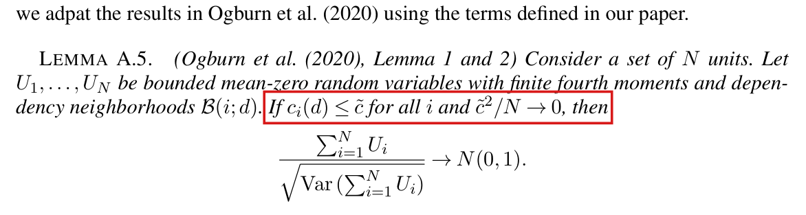
Let K(⋅)K(\cdot) in (19) be the uniform kernel with cutoff d~=h(d)\tilde d=h(d). Under C1–C5, and if N×AVar⁡(τ^HA(d))N\times\operatorname{AVar}(\widehat{\tau}_{\mathrm{HA}}(d)) is uniformly bounded away from zero for all large NN, the limit inferior of this interval’s coverage probability for AME⁡(d;η)\operatorname{AME}(d;\eta) is at least 1−α1-\alpha, for each 0<α<10<\alpha<1. Indeed, V^PDadj(d)≥V^PD(d)≥V^HAC(d)\widehat{V}^{\mathrm{adj}}_{\mathrm{PD}}(d)\ge\widehat{V}_{\mathrm{PD}}(d)\ge\widehat{V}_{\mathrm{HAC}}(d) and c≥z1−α/2c\ge z_{1-\alpha/2}, so the interval contains the interval of Proposition 4(ii) whenever V^HAC(d)≥0\widehat{V}_{\mathrm{HAC}}(d)\ge 0.

I have not assessed the finite-sample coverage of the capped interval. If the uncapped division is kept, Section 7 should present the interval as a finite-sample device supported by the simulations, and it should say that Proposition 4 does not cover it.

Six lines of body text. A red box marks the sentence: we recommend researchers to use the positive semidefinite HAC variance estimator with the empirical degree of adjustment when applying our method.
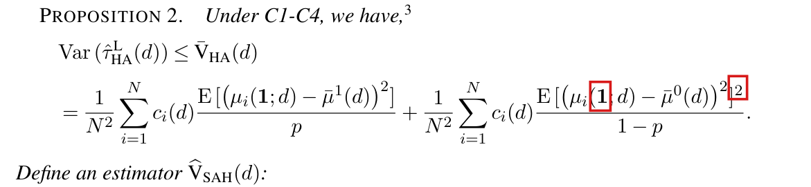
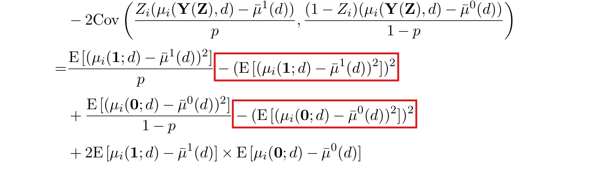
Section 7, p. 761 (PDF p. 18): the recommendation that closes the discussion of Figures 7 and 8.
Equation (44): mu equals the trace of (N1 N0 / N) M (Omega circ lambda-prime lambda) M. Below it a red box marks the sentence: The estimated variance is inflated by 1 over mu, becoming w-prime Sigma-hat HAC w over mu. Equation (45) for nu follows.
Supplement A, Section A.7, p. 17: equation (44) and the sentence that describes the rescaling of the variance. A.7 defines μ\mu with the uniform kernel matrix Ω\Omega only.
History of this entry
  1. Classification before my review (the classification when the audit was first completed, before I reviewed it): Moderate error.
  2. Revised. One sentence of what survives was qualified; the classification is unchanged (error, Moderate). How this came to light: a Lean formalization of Proposition 4 showed that, under its conditions, the coverage probabilities need not have limits, which the clarity note P004-N024 now records. Why it changed: the sentence said that Proposition 4 is correct as printed; it now refers to the proposition read with limits inferior, which is what the proof of the proposition supports and what this entry relies on. P. M. Aronow decided to add the clarity note; this note was written by the model session that runs the audit.

The Uganda script in the replication archive draws its randomization distribution by permuting treatment with a fixed count and no blocks, which is not the lottery within subcounties among covariate-balanced lists that assigned the villages; the same script measures HAC distances between centroids where footnote 3 prescribes minimal distances between polygons, and it uses twice the degrees of freedom of Supplement A.7.

Section 8.1, last paragraph of p. 763 (PDF p. 20), and Figure 11, p. 764; footnote 3, p. 751 (PDF p. 8); Supplement A, Section A.7, equation (45) and the sentence after it, p. 17; replication archive (Supplement B), application/scripts/Jayachandran_etal_2017.R, lines 111, 170–173, 286–289 and 339–342

As printed

Section 8.1, p. 763: “For the randomization test, we use 10,000 random draws, and the p-value is around 0.065.”

Footnote 3, p. 751: “As before, under point intervention, dij=γ(x(i),x(j))d_{ij}=\gamma(x(i),x(j)). Under polygon intervention, dij=min⁡x∈i,x′∈jγ(x,x′)d_{ij}=\min_{x\in i,x'\in j}\gamma(x,x').”

Supplement A, Section A.7, p. 17: equation (45),

ν=2∗Trace((N1N0NM(Ω∘(λ′λ))M)(N1N0NM(Ω∘(λ′λ))M)).\nu = 2 * \mathbf{Trace}\left(\left(\frac{N_1N_0}{N}\mathbf{M}\left(\Omega\circ(\lambda'\lambda)\right)\mathbf{M}\right)\left(\frac{N_1N_0}{N}\mathbf{M}\left(\Omega\circ(\lambda'\lambda)\right)\mathbf{M}\right)\right).

“We use the α2\frac{\alpha}{2}-quantile and (1−α2)\left(1-\frac{\alpha}{2}\right)-quantile of the t-distribution with 2μ2v\frac{2\mu^2}{v} degree of freedom to construct the confidence interval.”

Jayachandran_etal_2017.R, lines 111, 170, 286 and 341–342:

blockvar <- NULL

centr <- st_coordinates(st_centroid(map))

Zmat <- Zdata[, c(1:2)]

nu <- (nz/((nz-2)*XX_mat_inv[2, 2]))^2*sum(diag(dof_mat %*% dof_mat))\texttt{nu <- (nz/((nz-2)*XX\_mat\_inv[2, 2]))\textasciicircum 2*sum(diag(dof\_mat \%*\% dof\_mat))}

cvs[d] <- (2*dofs[d]^2) / nu\texttt{cvs[d] <- (}\colorbox{#ffe58a}{$\texttt{2*}$}\texttt{dofs[d]\textasciicircum 2) / nu}

The problem

I find three discrepancies in the script that the archive offers for Section 8.1.

The reference distribution. The test of Section 6.3 compares the observed statistic with its distribution over assignments drawn from the design. The script draws assignments uniformly among those with 60 treated villages out of 121, with no blocks. Note that fixing the number treated is not in itself an error: under Bernoulli assignment with a common probability, the assignment is uniform given its count. The trial was not assigned in that way. Its supplementary materials (Jayachandran et al., 2017, Section 2.2) describe a public lottery in each of seven subcounties. The villages of a subcounty were divided into two lists of nearly equal size, and only divisions balanced on four covariates were admitted: “For each subcounty, among the balanced permutations, we randomly chose one to use in the public lottery.” The lottery then selected the list to be treated. Permutations without blocks ignore both the subcounties and the balance restriction. The reference distribution of the script is not that of the trial, and the p-value it yields is not shown to be valid for the trial’s design.

The distances. Footnote 3 defines the distance between two polygons as the minimal distance between their points. The script computes these distances (lines 85–88) and then rebuilds the table of nodes Zdata from the centroids of the polygons (lines 170–173). The loop that computes the HAC intervals takes its distances from these centroids (lines 286–289). In the Uganda data, hundreds of pairs of villages that are within the kernel cutoff by polygon distance are beyond it by centroid distance.

The degrees of freedom. Section A.7 prescribes 2μ2/ν2\mu^2/\nu with ν\nu equal to twice the trace of the squared matrix, that is, the squared trace divided by the trace of the square. The script computes nu without the factor 2 and then sets cvs to 2 dofs2/nu2\,\texttt{dofs}^2/\texttt{nu}. The scalar normalization cancels in this ratio, and the result is twice the stated value, with or without the positive semidefinite trimming. More degrees of freedom give a smaller tt critical value and a narrower interval.

It is not established that this script produced Figure 11 or the p-value 0.0650.065. The stored results in the archive differ from the published ones (P004-N006).

Evidence an exact counterexample

For the reference distribution, the evidence is a check of the trial’s published design against the code. The article of Jayachandran et al. (2017) also states that the randomization was stratified by subcounty.

For the other two parts, the evidence is a pair of exact examples and a recalculation from the data in the archive. I take six nodes with Z=(0,1,0,1,0,1)Z=(0,1,0,1,0,1) and Y=(0,2,1,1,2,0)Y=(0,2,1,1,2,0) and an identity kernel. By A.7, I have 44 degrees of freedom, and the expressions in the script return 88. Next, I keep this assignment and these outcomes, place six rectangles of width 3 and height 1 on a line, with centres at 0,4,12,20,28,360,4,12,20,28,36, and take a cutoff of 2. The first two rectangles are at distance 11 as polygons and 44 as centroids, and no other pair is within the cutoff. The unadjusted HAC variance is 2/32/3 with polygon distances and 4/94/9 with centroid distances.

For the Uganda data at d=0d=0, the script’s calculation, done again from the data, reproduces the five stored pairs of interval endpoints to within 10−1210^{-12}. The first table compares the script’s degrees of freedom with those of A.7 and lists the half-widths at the stored standard errors. At the largest cutoff the upper endpoint of the stored interval moves from −0.00037-0.00037 to +0.00051+0.00051, so that this interval contains zero after the change. The second table counts the pairs of villages within the kernel cutoff. The cutoffs of the first table are those of the script, not those of Figure 11.

Uganda data, d=0d=0, stored estimate −0.01344-0.01344: degrees of freedom and half-widths of the 90% interval at the stored standard errors.
Nominal cutoff (km)df, scriptdf, A.7Half-width, scriptHalf-width, A.7Ratio
277.4877.4838.7438.740.011440.011440.011580.011581.0121.012
439.2839.2819.6419.640.014800.014800.015160.015161.0251.025
626.5126.5113.2613.260.015550.015550.016130.016131.0381.038
818.0518.059.039.030.014430.014430.015260.015261.0571.057
1015.5815.587.797.790.013070.013070.013950.013951.0671.067
Pairs of distinct villages within the kernel cutoff at d=0d=0, out of 7,260 pairs, by the script’s ellipsoidal centroid distances and by minimal spherical distances between polygons.
Kernel cutoff (km)By centroid distanceBy polygon distance
4309837
101,4802,154
203,3783,902
What survives

The polygon-distance rule in footnote 3 and the degrees-of-freedom formula in Section A.7 are correct; the estimand, the estimators and the theory under its stated assumptions are unaffected. Correcting the distances and the degrees of freedom changes neither the test statistic nor its reference distribution, and correcting the sampler does not change the intervals. The published p-value and the conclusion of no substantial leakage are not shown to be wrong: the computation behind the published numbers is not identified, and the direction of any change in those results is unknown. The theory in the paper assumes Bernoulli assignment. I have not examined how it extends to the restricted design of the trial.

Corrected
  • Draw reference assignments from the trial’s lottery: in each of the seven subcounties, choose with equal probability between its two original balanced lists, conditioning on those paired lists where available; otherwise reproduce their original selection procedure before the lottery. Setting blockvar to the subcounty alone does not reproduce this lottery.
  • In the loop over cutoffs, take the distances between villages as minimal distances between polygons, as in footnote 3, for the HAC kernel and for the degrees of freedom.
  • Replace line 342 by cvs[d] <- dofs[d]^2 / nu\texttt{cvs[d] <- }\colorbox{#ffe58a}{$\texttt{dofs[d]\textasciicircum 2}$}\texttt{ / nu}.
  • Compute the intervals and the p-value again before any published number is revised.
Five lines of body text and two footnotes. Red boxes mark the sentence: For the randomization test, we use 10,000 random draws, and the p-value is around 0.065.
Section 8.1, last paragraph of p. 763 (PDF p. 20): the randomization test and its p-value.
Two lines of body text and footnote 3. Red boxes mark the sentence: Under polygon intervention, d_ij = min over x in i and x-prime in j of gamma(x, x-prime).
Footnote 3, p. 751 (PDF p. 8): the distance between two polygons is the minimal distance between their points.
Equation (45): nu equals 2 times the trace of the square of the matrix (N1 N0 / N) M (Omega circ lambda-prime lambda) M, with a red box around the factor 2 and the star after it. Below it, the sentence that sets the degrees of freedom of the t-distribution, with a red box around the fraction 2 mu squared over v.
Supplement A, Section A.7, p. 17: equation (45) and the stated degrees of freedom, 2μ2/v2\mu^2/v with vv the ν\nu of (45).

The Uganda script in the replication archive projects the raster and the village polygons with a UTM zone of the central United States and then sends projected coordinates to a geodesic routine; its buffers of one unit are not buffers of one kilometre on the ground, and a projection for the study area with Euclidean distances, or geographic coordinates with geodesic distances, is needed.

Section 8.1, p. 763 (PDF p. 20), and Figure 11, p. 764 (PDF p. 21); replication archive (Supplement B), Jayachandran_etal_2017.R, lines 117 and 166–168, and SpatialEffect.R, lines 23–41 and 168–176

As printed

Section 8.1, p. 763: “To construct the circle averages, we generate buffers around each of the village polygons. The distance range for estimating the AME is set to run from zero km to 15 km.” Axes of Figure 11, p. 764: “Distance (km)”.

Jayachandran_etal_2017.R, lines 117 and 166–168:

dist.metric <- "Geodesic"

sr <- "+proj=utm +zone=15 +ellps=GRS80 +datum=NAD83 +units=km +no_defs"

ras <- projectRaster(ras, crs = sr)

ras_Z <- spTransform(ras_Z, crs(ras))

The problem

The villages lie near 31∘31^\circ E and 1∘1^\circ N, in UTM zone 36. The script projects the outcome raster and the polygons to UTM zone 15, which covers the central United States, with kilometre units. So far from its own zone the projection distorts lengths, and the package draws its buffers in the projected coordinates. A buffer of width one is then not a buffer of one km on the ground. Two points of the study area that are less than 1.1351.135 km apart on the ground are more than 1.991.99 units apart after projection, a ratio above 7/47/4. A point less than 0.6810.681 km from the boundary of the first village lies outside that village’s buffer of width one.

The script also selects geodesic distances. The package then takes the centroids of the projected polygons and passes their coordinates, in projected kilometres, to a routine that expects longitude and latitude in degrees. All 121 centroids have a first coordinate above 360, and the routine stops with the error longitude > 360. This path cannot produce HAC distances. The later block of the script, which computes the intervals for the varying cutoffs, uses the original geographic coordinates and valid geodesic distances, and this defect does not reach it.

No dependence of Figure 11 on this path is established. If the published analysis used these buffers, every estimate at a nonzero distance and the cumulative statistic refer to regions other than those stated.

Evidence an exact counterexample

I checked the projection’s returned coordinates by exact comparisons, with an analytic upper bound for distances on the ground, after bypassing the separate execution errors; I did not reproduce the estimates. The first centroid is sent to the routine as about (8019,19696)(8019, 19696), and all 121 fail its bounds of 360 and 90. The table lists the two comparisons of distances. The first uses the points at longitudes 31.2∘31.2^\circ and 31.21∘31.21^\circ E on the parallel 1.2∘1.2^\circ N. With a projection for UTM zone 36 the same two points are 1.1131.113 units apart, and their geodesic distance is 1.1131.113 km. The second uses a boundary vertex of the first village and the point 0.006∘0.006^\circ west of it on the same parallel.

Distances on the ground and in the projected coordinates of the script.
PairOn the groundIn the script’s projection
Two points 0.01∘0.01^\circ of longitude apartless than 1.1351.135 kmmore than 1.991.99 units
A point and the first villageless than 0.6810.681 kmmore than 11 unit (outside the buffer)
What survives

These code defects do not refute the definitions of distance or the statistical theory. The region at distance zero is the village itself and needs no positive buffer width; I have not verified its published numerical estimate. Figure 11, the cumulative statistic, its p-value and the conclusion about leakage are not shown to depend on this path: the script as supplied does not run against the package supplied with it (P004-E029), and the code that produced Figure 11 is not identified. What changes is that the archive cannot confirm the distance scale of Figure 11.

Corrected

sr <- "+proj=utm +zone=36 +datum=WGS84 +units=km +no_defs"

dist.metric <- "Euclidean"

Transform the raster and the polygons with the same projection, using transformations appropriate to their classes, and compute distances and buffers in the projected kilometres. This is a local approximation to ground distances. The alternative is to keep geographic coordinates with geodesic distances and to bring the buffer widths (in metres), the distances and the cutoffs to the same unit. The separate script/package interface errors also need repair (P004-E029). Any result obtained from the buffers of the supplied script should be computed again.

Six lines of body text. Red boxes mark the two sentences: To construct the circle averages, we generate buffers around each of the village polygons. The distance range for estimating the AME is set to run from zero km to 15 km.
Section 8.1, p. 763 (PDF p. 20): the buffers around the village polygons and the range of distances, in km.
Figure 11 with its caption. Two panels, Hajek Estimator on the left and Smoothed Hajek Estimator (Triangular Kernel, bw=5km) on the right, each showing an effect curve near zero with upper and lower interval curves for cutoffs of 2, 5 and 10 km, over distances from 0 to about 14 km. Red boxes mark the label Distance (km) under each horizontal axis.
Figure 11, p. 764 (PDF p. 21). Both panels plot the estimates against distance in km; the marks show the two axis labels.

Minor (33)

Real but inconsequential, for example a misprint that does not change a result.

Lemma A.6 needs the true coefficient θ0\theta_0 to be an interior point of the compact set Θ0\Theta_0 over which the likelihood is maximized; when θ0\theta_0 lies on the boundary of Θ0\Theta_0, the expansion of the estimator fails.

Supplement A, Appendix A.6, condition C 1, items (iv) and (vi), and Lemma A.6, p. 14 (C 1 begins on p. 13)

See also under Formal statements (Lean): P004-T9, P004-T10

As printed

(iv) Compact Parameter Space: θ0∈Θ0\colorbox{#ffe58a}{$\theta_0\in\Theta_0$} where Θ0⊂Rk\Theta_0\subset\mathbb R^k is a compact set.

(vi) The MLE estimator is used to estimate the coefficient vector θ\theta:

θ^MLE=arg⁡max⁡θ∈Θ0∑i=1N(ZiOi′θ−log⁡(1+exp⁡(Oi′θ))).\widehat\theta_{MLE}=\arg\max_{\theta\in\Theta_0}\sum_{i=1}^{N}\bigl(Z_iO_i'\theta-\log(1+\exp(O_i'\theta))\bigr).

Lemma A.6. Under C6 and C1, θ^MLE−θ0=op(1)\widehat\theta_{MLE}-\theta_0=o_p(1) and

θ^MLE−θ0=(1N∑i=1Np(Oi∣θ0)(1−p(Oi∣θ0))OiOi′)−11N∑i=1N((Zi−p(Oi∣θ0))Oi)+op(N−12).\widehat\theta_{MLE}-\theta_0=\Bigl(\frac1N\sum_{i=1}^{N}p(O_i\mid\theta_0)(1-p(O_i\mid\theta_0))O_iO_i'\Bigr)^{-1}\frac1N\sum_{i=1}^{N}\bigl((Z_i-p(O_i\mid\theta_0))O_i\bigr)\colorbox{#ffe58a}{$\displaystyle +o_p(N^{-\frac12})$}.

In particular, θ^MLE−θ0=Op(N−12)\widehat\theta_{MLE}-\theta_0=O_p(N^{-\frac12}).

The problem

The estimator is defined as the maximizer of the likelihood over Θ0\Theta_0, and item (iv) only places θ0\theta_0 in Θ0\Theta_0. A value of θ0\theta_0 on the boundary of Θ0\Theta_0 is therefore allowed. There the constrained maximizer need not solve the score equation, and the expansion of Lemma A.6, which is the expansion of an unconstrained maximizer, fails. Condition C6 concerns independence and overlap and does not restrict Θ0\Theta_0.

Evidence an exact counterexample

The evidence is an exact counterexample and a derivation of the lemma under the corrected condition.

Counterexample. Let k=1k=1, Oi=1O_i=1, Θ0=[0,1]\Theta_0=[0,1] and θ0=0\theta_0=0, and let the ZiZ_i be independent with probability 1/21/2. Every item of C 1 holds (with bound 1 on the confounder and Gram matrix 1), and C6 holds with ϵ=1/4\epsilon=1/4. Let T=∑i(2Zi−1)T=\sum_i(2Z_i-1). The matrix of the lemma equals 1/41/4, and the leading term is 2T/N2T/N. The derivative of the log-likelihood at 0 is T/2T/2, and the log-likelihood is strictly concave. If T<0T<0, it is decreasing on [0,1][0,1] and θ^MLE=0\widehat\theta_{MLE}=0 exactly. On this event the remainder of the lemma is −2T/N-2T/N, and N\sqrt N times its absolute value exceeds 1 when in addition T2>N/4T^2>N/4. Since E[T2]=NE[T^2]=N and E[T4]=3N2−2NE[T^4]=3N^2-2N, the Cauchy–Schwarz inequality implies that

Pr⁡(T2>N/4)≥(3N/4)23N2−2N≥316,\Pr\bigl(T^2>N/4\bigr)\ge\frac{(3N/4)^2}{3N^2-2N}\ge\frac{3}{16},

and the distribution of TT is symmetric. I conclude that

Pr⁡(N ∣θ^MLE−θ0−2T/N∣>1)≥332for every N≥1,\Pr\Bigl(\sqrt N\,\bigl|\widehat\theta_{MLE}-\theta_0-2T/N\bigr|>1\Bigr)\ge\frac{3}{32}\quad\text{for every }N\ge1,

so that the remainder is not op(N−1/2)o_p(N^{-1/2}). The limit of N θ^MLE\sqrt N\,\widehat\theta_{MLE} is 2max⁡{U,0}2\max\{U,0\} with UU standard normal, and the leading term has the limit 2U2U.

The lemma for an interior θ0\theta_0. Let gN=N−1∑i(Zi−pi)Oig_N=N^{-1}\sum_i(Z_i-p_i)O_i and δ=θ^MLE−θ0\delta=\widehat\theta_{MLE}-\theta_0, and let ℓN\ell_N be the log-likelihood divided by NN. Under C 1 and C6, I have gN=Op(N−1/2)g_N=O_p(N^{-1/2}), and there exists a constant c>0c>0 such that the negative Hessian of ℓN\ell_N is at least cc times the identity on every segment between two points of Θ0\Theta_0. Since θ0∈Θ0\theta_0\in\Theta_0, I obtain

0≤ℓN(θ^MLE)−ℓN(θ0)≤gN′δ−c2∥δ∥2,0\le\ell_N(\widehat\theta_{MLE})-\ell_N(\theta_0)\le g_N'\delta-\frac c2\|\delta\|^2,

which implies that ∥δ∥≤2∥gN∥/c=Op(N−1/2)\|\delta\|\le2\|g_N\|/c=O_p(N^{-1/2}). This part uses the printed conditions only. If the ball B(θ0,r)B(\theta_0,r) lies in Θ0\Theta_0, then ∥δ∥<r/2\|\delta\|<r/2 with probability tending to one. On that event the maximizer is an interior point and the score vanishes there, so that 0=gN−HNδ+eN0=g_N-H_N\delta+e_N with ∥eN∥≤C∥δ∥2\|e_N\|\le C\|\delta\|^2, where HNH_N is the matrix of the lemma. Since HN−1H_N^{-1} is bounded, I find δ=HN−1gN+Op(N−1)\delta=H_N^{-1}g_N+O_p(N^{-1}).

What survives

The first and the last assertion of Lemma A.6, consistency and the rate Op(N−1/2)O_p(N^{-1/2}), hold under the printed conditions, boundary included. The results for experiments with a known assignment probability do not use the lemma. The script of the observational application fits the logistic model without a constraint on the coefficient. This example does not establish any change to its reported numbers. What depends on the corrected condition is the expansion of Lemma A.6 and the results of A.6 that use it. If fixed outcomes are added to the boundary example, equation (36) and the normal limit of Proposition 4 of A.6 fail as well, although NN times the variance of the printed linear form equals 4. That proposition has a second and separate defect, treated in P004-E001.

Corrected

(iv) Compact Parameter Space: θ0\theta_0 is an interior point of Θ0\Theta_0, where Θ0⊂Rk\Theta_0\subset\mathbb R^k is a fixed compact set. That is, there exists a fixed r>0r>0 such that the ball B(θ0,r)B(\theta_0,r) is contained in Θ0\Theta_0.

Lemma A.6. Under C6 and C 1 with item (iv) as above, θ^MLE−θ0=op(1)\widehat\theta_{MLE}-\theta_0=o_p(1) and

θ^MLE−θ0=(1N∑i=1Np(Oi∣θ0)(1−p(Oi∣θ0))OiOi′)−11N∑i=1N(Zi−p(Oi∣θ0))Oi+op(N−12).\widehat\theta_{MLE}-\theta_0=\Bigl(\frac1N\sum_{i=1}^{N}p(O_i\mid\theta_0)(1-p(O_i\mid\theta_0))O_iO_i'\Bigr)^{-1}\frac1N\sum_{i=1}^{N}(Z_i-p(O_i\mid\theta_0))O_i+o_p(N^{-\frac12}).

In particular, θ^MLE−θ0=Op(N−12)\widehat\theta_{MLE}-\theta_0=O_p(N^{-\frac12}). The remainder in the display is Op(N−1)O_p(N^{-1}).

Crop of items (iv), (v) and (vi) of a condition and of Lemma A.6. Item (iv) reads: Compact Parameter Space: theta-zero in Theta-zero where Theta-zero, a subset of R to the k, is a compact set. Item (vi) defines theta-hat-MLE as the maximizer over theta in Theta-zero of the logistic log-likelihood. Lemma A.6 reads: Under C6 and C1, theta-hat-MLE minus theta-zero is o-p of 1, and theta-hat-MLE minus theta-zero equals the inverse of the average of p times 1 minus p times O sub i O sub i prime, times the average of Z sub i minus p times O sub i, plus o-p of N to the minus one half. In particular, theta-hat-MLE minus theta-zero is O-p of N to the minus one half. One red outline surrounds theta-zero in Theta-zero in item (iv). A second surrounds the term plus o-p of N to the minus one half.
Supplement A, condition C 1, items (iv) to (vi), and Lemma A.6, p. 14. The outlines mark the condition on θ0\theta_0 and the remainder of the expansion.

In the Horvitz–Thompson estimator for observational studies, the control observations are weighted by 1/(1−p(Oi))1/(1-p(O_i)), not by 1/p(Oi)1/p(O_i).

Section 6.4, display that defines τ^HTobs(d)\widehat\tau^{obs}_{HT}(d), p. 759 (PDF p. 16); Supplement A, A.1.3, last line of the display, p. 4

See also under Formal statements (Lean): P004-T11

As printed

Main text, p. 759. Under C6 the Horvitz–Thompson estimator with known propensity scores, defined as

τ^HTobs(d)=1N∑i=1NZip(Oi)μi(Y;d)−1N∑i=1N1−Zip(Oi)μi(Y;d),\widehat\tau^{\mathrm{obs}}_{\mathrm{HT}}(d)=\frac1N\sum_{i=1}^{N}\frac{Z_i}{p(O_i)}\mu_i(\mathbf Y;d)-\frac1N\sum_{i=1}^{N}\frac{1-Z_i}{\colorbox{#ffe58a}{$\displaystyle p(O_i)$}}\mu_i(\mathbf Y;d),

is unbiased for AME(d;η)\mathrm{AME}(d;\eta).

Supplement A, p. 4, last line of the display.

=E[1N∑i=1NZip(Oi)μi(Y;d)−1N∑i=1N1−Zip(Oi)μi(Y;d)]=\mathrm E\Bigl[\frac1N\sum_{i=1}^{N}\frac{Z_i}{p(O_i)}\mu_i(\mathbf Y;d)-\frac1N\sum_{i=1}^{N}\frac{1-Z_i}{\colorbox{#ffe58a}{$\displaystyle p(O_i)$}}\mu_i(\mathbf Y;d)\Bigr]
The problem

As printed, the control observations are weighted by the inverse of the probability of treatment. The estimator so defined is not unbiased for the AME in general. The line before the last one in the proof of A.1.3 has the factor (1−p(Oi))/(1−p(Oi))(1-p(O_i))/(1-p(O_i)) for the control arm, and the IPW estimator of A.6 (Supplement A, p. 14) has the denominator 1−p(Oi∣θ^MLE)1-p(O_i\mid\widehat\theta_{MLE}). The denominator p(Oi)p(O_i) in the control sum is a misprint that occurs in both places.

Evidence a derivation

The evidence is a derivation. Let pi=p(Oi)p_i=p(O_i) and mia=E[μi(Y;d)∣Zi=a]m_{ia}=E[\mu_i(\mathbf Y;d)\mid Z_i=a], which is μi(a;d,η)\mu_i(a;d,\eta) in the notation of A.1.3. Then AME(d;η)=N−1∑i(mi1−mi0)\mathrm{AME}(d;\eta)=N^{-1}\sum_i(m_{i1}-m_{i0}). Under C6, I have 0<pi<10<p_i<1 and

E[Ziμi(Y;d)pi]=mi1,E[(1−Zi)μi(Y;d)pi]=(1−pi)mi0pi,E[(1−Zi)μi(Y;d)1−pi]=mi0.E\Bigl[\frac{Z_i\mu_i(\mathbf Y;d)}{p_i}\Bigr]=m_{i1},\qquad E\Bigl[\frac{(1-Z_i)\mu_i(\mathbf Y;d)}{p_i}\Bigr]=\frac{(1-p_i)m_{i0}}{p_i},\qquad E\Bigl[\frac{(1-Z_i)\mu_i(\mathbf Y;d)}{1-p_i}\Bigr]=m_{i0}.

The printed estimator has expectation N−1∑i[mi1−(1−pi)mi0/pi]N^{-1}\sum_i[m_{i1}-(1-p_i)m_{i0}/p_i], and the corrected one has expectation AME(d;η)\mathrm{AME}(d;\eta). For example, if μi(Y;d)=1\mu_i(\mathbf Y;d)=1 for every assignment and pi=1/4p_i=1/4, then the AME is 0, the printed estimator has expectation 1−3=−21-3=-2, and the corrected one has expectation 0.

What survives

The corrected estimator is unbiased under C6, and the proof in A.1.3 is correct up to its last line. The IPW estimator of A.6 is defined with the correct weight. The inference for that estimator is a separate matter, treated in P004-E001.

Corrected

Under C6 the Horvitz–Thompson estimator with known propensity scores, defined as

τ^HTobs(d)=1N∑i=1NZip(Oi)μi(Y;d)−1N∑i=1N1−Zi1−p(Oi)μi(Y;d),\widehat\tau^{obs}_{HT}(d)=\frac1N\sum_{i=1}^{N}\frac{Z_i}{p(O_i)}\mu_i(\mathbf Y;d)-\frac1N\sum_{i=1}^{N}\frac{1-Z_i}{\colorbox{#ffe58a}{$\displaystyle 1-p(O_i)$}}\mu_i(\mathbf Y;d),

is unbiased for AME(d;η)\mathrm{AME}(d;\eta). The last line of the display in Supplement A.1.3 (p. 4) has the same denominator 1−p(Oi)1-p(O_i) in its second sum.

Crop of three lines of text, a displayed formula and one more line. The text ends: Under C6 the Horvitz-Thompson estimator with known propensity scores, defined as. The formula reads: tau-hat-obs sub HT of d equals one over N times the sum over i of Z sub i over p of O sub i times mu sub i of Y and d, minus one over N times the sum over i of 1 minus Z sub i over p of O sub i times mu sub i of Y and d. The line below reads: is unbiased for AME of d and eta. A red outline surrounds the denominator p of O sub i of the second fraction.
Section 6.4, p. 759 (PDF p. 16). The outline marks the denominator of the control term, printed as p(Oi)p(O_i).
Crop of three displayed lines and one line of text. The first two lines carry, for the control arm, the fraction 1 minus p of O sub i over 1 minus p of O sub i. The third line reads: equals E of one over N times the sum of Z sub i over p of O sub i times mu sub i of Y and d, minus one over N times the sum of 1 minus Z sub i over p of O sub i times mu sub i of Y and d. A red outline surrounds the denominator p of O sub i of the second fraction in the third line. The text below reads: The fourth equality uses C6-(ii) and the law of total expectations.
Supplement A, A.1.3, p. 4, last three lines of the display. The line before the last has 1−p(Oi)1-p(O_i) for the control arm; the outline marks the denominator p(Oi)p(O_i) in the last line.

The Monte Carlo rule compares ∣T(Y,Zp)∣|T(\mathbf Y,\mathbf Z_p)| with ∣T(Y,Z)∣|T(\mathbf Y,\mathbf Z)|, and it has level α\alpha for every number PP of draws when the observed assignment is counted, that is, when one rejects if (1+B)/(P+1)≤α(1+B)/(P+1)\le\alpha, where BB is the number of draws whose statistic is at least as extreme as the observed one.

Section 6.3, second paragraph, p. 758 (PDF p. 15)

See also under Formal statements (Lean): P004-T12, P004-T13

As printed

As a result, rejecting the null if 1P∑p1{∣T(Y,Zp)∣≥T(Y,Z)}≤α\frac{1}{P}\sum_p \mathbf 1\{|T(\mathbf Y,\mathbf Z_p)|\ge \colorbox{#ffe58a}{$T(\mathbf Y,\mathbf Z)$}\}\le\alpha for some fixed large enough PP gives an α\alpha-level exact test of the sharp null hypothesis.

The problem

There are two points. First, the indicator compares the absolute value of each simulated statistic with the signed observed statistic. If T(Y,Z)<0T(\mathbf Y,\mathbf Z)<0, then every indicator equals 1, the proportion is 1, and the rule cannot reject. The statistics of the paper are signed. In Section 8.1 the observed statistic is −0.034-0.034 and the reported pp-value is about 0.065, which the printed rule cannot produce. The comparison that is meant has ∣T(Y,Z)∣|T(\mathbf Y,\mathbf Z)| on the right.

Second, let BB be the number of draws with ∣T(Y,Zp)∣≥∣T(Y,Z)∣|T(\mathbf Y,\mathbf Z_p)|\ge|T(\mathbf Y,\mathbf Z)|. The rule that rejects when B/P≤αB/P\le\alpha does not have level α\alpha merely because PP is large. Its size can exceed α\alpha at a given PP, by at most (1−α)/(P+1)(1-\alpha)/(P+1).

Evidence an exact counterexample

The evidence is an exact counterexample to the level of the rule B/P≤αB/P\le\alpha, computed in rational arithmetic, and a derivation of the level of the corrected rule.

Example. I take eight intervention nodes at the points (3i,0)(3i,0), i=1,…,8i=1,\dots,8, with one outcome point at each node, and the outcomes yi=2i−8y_i=2^{i-8}, that is, 1/128,1/64,…,11/128,1/64,\dots,1, under every assignment. The sharp null hypothesis holds. The assignments are independent with probability 1/21/2, and the statistic is the absolute value of the Horvitz–Thompson estimator (13) at d=0d=0. The 256 assignments yield the 128 values (2r−1)/512(2r-1)/512, r=1,…,128r=1,\dots,128, each with probability 1/1281/128. Let α=1/20\alpha=1/20 and P=100P=100. If the observed statistic is the mmth largest value, then BB is binomial with parameters 100100 and m/128m/128, and the rule rejects when B≤5B\le5. Summing over mm, I obtain the size

1128∑m=1128Pr⁡(Bin⁡(100,m/128)≤5)=0.0555…>120.\frac{1}{128}\sum_{m=1}^{128}\Pr\bigl(\operatorname{Bin}(100,m/128)\le5\bigr)=0.0555\ldots>\frac1{20}.

The rule with (1+B)/(P+1)(1+B)/(P+1) rejects when B≤4B\le4 and has size 0.0456…0.0456\ldots in the same design. For the signed estimator with the comparison as printed, the 128 assignments with a negative estimate never reject, and the size is 0.0277…0.0277\ldots, half of the first value.

A large number of draws. With 17 nodes and yi=2i−17y_i=2^{i-17} there are M=65536M=65536 equally likely values of the statistic. For P=10000P=10000 and α=1/20\alpha=1/20 the rule rejects when B≤500B\le500. If the observed statistic is the mmth largest value, the rule rejects with probability f(m/M)f(m/M), where f(q)=Pr⁡(Bin⁡(10000,q)≤500)f(q)=\Pr(\operatorname{Bin}(10000,q)\le500) is decreasing in qq and has integral 501/10001501/10001 over [0,1][0,1]. Comparing the sum over mm with the integral, I find that the size is at least

50110001−165536=32823535655425536=0.05008…>120.\frac{501}{10001}-\frac{1}{65536}=\frac{32823535}{655425536}=0.05008\ldots>\frac1{20}.

The corrected rule. Let S0=∣T(Y,Z)∣S_0=|T(\mathbf Y,\mathbf Z)| and Sp=∣T(Y,Zp)∣S_p=|T(\mathbf Y,\mathbf Z_p)| for p=1,…,Pp=1,\dots,P. Under the sharp null hypothesis the outcomes are fixed, and S0,S1,…,SPS_0,S_1,\dots,S_P are independent and identically distributed. Let RiR_i be the number of indices jj with Sj≥SiS_j\ge S_i. Then the corrected pp-value is R0/(P+1)R_0/(P+1). For any values and any integer kk, at most kk indices have Ri≤kR_i\le k, since such an index is among the kk largest values, ties included. Taking k=⌊α(P+1)⌋k=\lfloor\alpha(P+1)\rfloor and using that the P+1P+1 indices are exchangeable, I have

(P+1)Pr⁡(R0P+1≤α)=E[∑i=0P1{Ri≤k}]≤k≤α(P+1).(P+1)\Pr\Bigl(\frac{R_0}{P+1}\le\alpha\Bigr)=E\Bigl[\sum_{i=0}^{P}\mathbf 1\{R_i\le k\}\Bigr]\le k\le\alpha(P+1).

Applying the same argument to the event B≤⌊αP⌋B\le\lfloor\alpha P\rfloor, I obtain Pr⁡(B/P≤α)≤(⌊αP⌋+1)/(P+1)≤α+(1−α)/(P+1)\Pr(B/P\le\alpha)\le(\lfloor\alpha P\rfloor+1)/(P+1)\le\alpha+(1-\alpha)/(P+1).

What the examples do not show. The rule B/P≤αB/P\le\alpha is not invalid for every PP. For α=1/20\alpha=1/20 and P=9999P=9999 both rules reject exactly when B≤499B\le499. For a fixed finite design the rule becomes conservative when PP is large enough: in the eight-node example its size is at most 1997/400001997/40000 for all P≥8,000,000P\ge8{,}000{,}000. If the printed sentence only asserts that a suitable PP exists, these examples do not contradict it. What fails is the guarantee for an arbitrary large PP.

What survives

The definitions of the AME, the point estimators, their limit theory and the confidence intervals do not use this rule. The simulation code in the replication files takes absolute values on both sides and compares the observed statistic with a quantile of the simulated ones, so the printed comparison is not what was computed, and no curve of Figure 9 is shown to be wrong. The separate recalculations in P004-N006 do not identify the computation behind the reported pp-value of Section 8.1. If it is B/PB/P with P=10,000P=10{,}000, then the corrected value exceeds it by at most 1/100011/10001, and the rejection at the 10% level and the non-rejection at the 5% level are unchanged. The corrected rule needs no new assumption. The pp-value increases by (1−B/P)/(P+1)(1-B/P)/(P+1).

Corrected

Under the sharp null hypothesis, draw Z1,…,ZP\mathbf Z_1,\dots,\mathbf Z_P independently from the assignment distribution of the experiment, independently of the observed assignment Z\mathbf Z. Reject the null if

1+∑p=1P1{∣T(Y,Zp)∣≥∣T(Y,Z)∣}P+1≤α.\frac{\colorbox{#ffe58a}{$\displaystyle 1+$}\sum_{p=1}^{P}\mathbf 1\{|T(\mathbf Y,\mathbf Z_p)|\ge \colorbox{#ffe58a}{$\displaystyle |T(\mathbf Y,\mathbf Z)|$}\}}{\colorbox{#ffe58a}{$\displaystyle P+1$}}\le\alpha .

For every P≥1P\ge1 this is a test of the sharp null hypothesis whose size is at most α\alpha in finite samples. Ties and the discreteness of the randomization distribution can make it conservative. A larger PP gives a finer pp-value and is not needed for the level.

Crop of six lines of text from Section 6.3. The fourth and fifth lines read: under the sharp null. As a result, rejecting the null if one over P times the sum over p of the indicator that the absolute value of T of Y and Z sub p is at least T of Y and Z, is at most alpha, for some fixed large enough P gives an alpha-level exact test of the sharp null hypothesis. One red outline surrounds T of Y and Z on the right of the inequality inside the indicator. A second surrounds the words alpha-level exact test.
Section 6.3, second paragraph, p. 758 (PDF p. 15). The outlines mark the observed statistic, which is printed without an absolute value, and the words “α\alpha-level exact test”.

The disk and donut AMEs are not special cases of the smoothed AME (26) with uniform kernels: they weight each distance by the mass of outcome points at that distance from each node.

Section 6.2, p. 757 (PDF p. 14), the sentence after equation (26)

See also under Formal statements (Lean): P004-T14, P004-T15

As printed

“The donut and disk AMEs, defined in Section 3, are special cases with (properly-normalized) uniform kernels.”

The problem

By (2), a disk or donut average is the integral of the outcome over the points whose distance to the node lies in a band, divided by the mass of those points under the measure ζ\zeta. Each distance in the band then enters with a weight equal to the mass of outcome points at that distance from the node. Equation (26) averages the circle AMEs over distance with one kernel, common to all nodes. A kernel that is constant on the band gives every distance the same weight, and no normalization of it supplies weights that vary with the distance or with the node. For a point node under area measure, the weight of radius rr in the disk [0,d][0,d] is 2r/d22r/d^2, not 1/d1/d.

Evidence an exact counterexample

The evidence is three exact calculations and a derivation. First, I consider one node at the origin, independent Bernoulli(1/2)(1/2) assignment, and unit mass at each of the outcome points (1,0)(1,0), (0,2)(0,2) and (−2,0)(-2,0), with effects 00, 11 and 11. The circle AMEs at radii 11 and 22 are 00 and 11, and their uniform average is 1/21/2. The disk [0,2][0,2] and the donut [1,2][1,2] each have AME 2/32/3. Second, I consider nodes at (0,0)(0,0) and (3,0)(3,0) and unit mass at (0,4)(0,4), (3,4)(3,4) and (3,−4)(3,-4), with Yx(z)=1+z1g1(x)+z2g2(x)Y_x(\mathbf z)=1+z_1g_1(x)+z_2g_2(x), g1=(0,1,1)g_1=(0,1,1) and g2=(−1,0,0)g_2=(-1,0,0). Then AME(4)=AME(5)=0\mathrm{AME}(4)=\mathrm{AME}(5)=0, and every choice of common weights on the two radii gives 00. The AME of the disk [0,5][0,5] and of the donut [4,5][4,5] equals 1/61/6. The normalized masses at radii 44 and 55 are (1/3,2/3)(1/3,2/3) for the first node and (2/3,1/3)(2/3,1/3) for the second. Third, for one point node, area measure on the unit disk and Yx(z)=z∥x∥Y_x(z)=z\|x\|, the circle AME at radius rr is rr. Its uniform average over [0,1][0,1] is 1/21/2, and the disk AME is 2/32/3.

For the derivation, let δi(x)\delta_i(x) be the marginalized effect of node ii on the point xx. By (6), (8) and (9), the effect of node ii on a band DD is ∫di(x)∈Dδi(x) ζ(dx)\int_{d_i(x)\in D}\delta_i(x)\,\zeta(dx) divided by ζ{x:di(x)∈D}\zeta\{x:d_i(x)\in D\}. Rewriting the integral over xx as an integral over the distance r=di(x)r=d_i(x), I obtain the formula of the corrected passage.

What survives

Definitions (2), (6), (8) and (9), the inference results of Section 5 and the smoothed quantities (26) and (27) are unaffected. Equations (26) and (27) still define smoothed quantities, and the applications report smooths with a triangular kernel. No reported number depends on the sentence. What is withdrawn is the identity between a disk or donut AME and the smoothed AME (26) with a uniform kernel. When the masses at each distance differ across nodes, the circle AMEs alone need not determine the AME of a disk or donut. The reading of a sum of ring estimates as an area effect in Section 8.1 is the subject of P004-E008.

Corrected

“The donut and disk AMEs average the node-specific circle effects over their distance bands using the normalized shell-mass measures induced by the spatial measure. For complete Euclidean disks about point interventions under area weighting, these radial weights are proportional to distance; a common uniform radial kernel applies as an identity only when the normalized shell-mass measures coincide with it.”

Precisely, for a node ii and a set AA of distances let νi(A)=ζ{x:di(x)∈A}\nu_i(A)=\zeta\{x:d_i(x)\in A\}, and let τi(r;η)\tau_i(r;\eta) be the effect of node ii on the outcome points at distance rr (for a measure without atoms, the conditional effect given the distance). For a band DD such that 0<νi(D)<∞0<\nu_i(D)<\infty for all ii,

AMED(η)=1N∑i=1N∫Dτi(r;η) νi(dr)νi(D).\mathrm{AME}_D(\eta)=\frac1N\sum_{i=1}^N\frac{\int_D\tau_i(r;\eta)\,\nu_i(dr)}{\nu_i(D)}.

For a complete Euclidean disk about a point node under area measure, the normalized measure νi(dr)/νi(D)\nu_i(dr)/\nu_i(D) has density 2r/d22r/d^2 on D=[0,d]D=[0,d] and density 2r/(b2−a2)2r/(b^2-a^2) on an annulus D=[a,b]D=[a,b].

Crop of equation (26), sAME(d; eta) equal to the integral over t of AME(t; eta) times K_h((d minus t) over h), and of the six lines of text after it. A red box marks the sentence 'The donut and disk AMEs, defined in Section 3, are special cases with (properly-normalized) uniform kernels.'
Section 6.2, p. 757 (PDF p. 14), equation (26) and the paragraph after it. The marked sentence calls the donut and disk AMEs special cases of the smoothed AME (26) with uniform kernels.

The Costa Rica outcome is deforestation by 1997; the year 1980 is the cutoff for the establishment of the protected areas, not the date of the outcome.

Section 8.2, first paragraph, p. 764 (PDF p. 21)

As printed

“The outcome is measured at the level of parcels with a size of three hectares. Each parcel has a value of 1 if deforestation occurred inside it before 1980.”

The problem

The sentence assigns to the outcome the date that defines the treatment. In the study that Section 8.2 cites, each parcel is classified as deforested or forested at the end year, 1997 for Costa Rica, and 1980 is the cutoff for the establishment of the protected areas.

Evidence a derivation

The evidence is a check of the cited source. Ferraro, Hanauer and Sims (2011), p. 13914, write: “Each parcel is classified as deforested or forested by the end year (Costa Rica in 1997 and Thailand in 2000)”, and they describe the protected areas as “established before 1980 (Costa Rica)”. The application script in the replication archive takes its outcome from a field named defor97.

What survives

This correction changes the description only. The script uses defor97, and no estimate, interval or figure has been shown wrong by this date check. I did not compute the Costa Rica results again.

Corrected

“Each parcel has a value of 1 if deforestation occurred inside it by 1997.”

If the sample is described further, the protected areas are those established before 1980.

The first paragraph of Section 8.2, nine lines of body text. A red box marks the words before 1980 in the sentence: Each parcel has a value of 1 if deforestation occurred inside it before 1980.
Section 8.2, first paragraph, p. 764 (PDF p. 21): the definition of the outcome of the Costa Rica application.

In Lemma A.3 the control sum of the linearised Hajek estimator should be divided by N(1−p)N(1-p), not by NpNp.

Supplement A, Lemma A.3, p. 4, displayed linear expansion

See also under Formal statements (Lean): P004-T18, P004-T42, P004-T44

As printed

Lemma A.3. Consider the estimator τ^HA(d)\widehat\tau_{\mathrm{HA}}(d) defined in (16). It has the following asymptotic linear expansion:

τ^HAL(d)=AME(d;η)+1Np∑i=1NZi(μi(Y(Z);d)−μˉ1(d))−1Np∑i=1N(1−Zi)(μi(Y(Z);d)−μˉ0(d)).\widehat\tau^{\mathrm{L}}_{\mathrm{HA}}(d)=\mathrm{AME}(d;\eta)+\frac{1}{Np}\sum_{i=1}^N Z_i\left(\mu_i(\mathbf{Y}(\mathbf{Z});d)-\bar\mu^1(d)\right)-\frac{1}{\colorbox{#ffe58a}{$\displaystyle Np$}}\sum_{i=1}^N(1-Z_i)\left(\mu_i(\mathbf{Y}(\mathbf{Z});d)-\bar\mu^0(d)\right).

Such an expansion satisfies N(τ^HAL(d)−τ^HA(d))=op(1)\sqrt{N}\left(\widehat\tau^{\mathrm{L}}_{\mathrm{HA}}(d)-\widehat\tau_{\mathrm{HA}}(d)\right)=o_p(1).

The problem

The proof of the lemma writes the Hajek estimator as f(a,b,c,d)=a/c−b/df(a,b,c,d)=a/c-b/d evaluated at the treated and control averages and the two normalised counts, and it defines the control average and the control count with the factor 1/(N(1−p))1/(N(1-p)). The first-order term of that expansion divides the control residuals by N(1−p)N(1-p). The statement prints NpNp. The two expressions agree when p=1/2p=1/2. For other values of pp the printed expansion does not in general satisfy the last sentence of the lemma: its difference from the Hajek estimator is of order N−1/2N^{-1/2} and not smaller.

Evidence a derivation

The evidence is a derivation and an exact counterexample to the printed display. In the notation of the proof,

μ^1(d)=1Np∑i=1NZiμi,μ^0(d)=1N(1−p)∑i=1N(1−Zi)μi,N^1=1Np∑i=1NZi,N^0=1N(1−p)∑i=1N(1−Zi),\begin{aligned} \widehat\mu^1(d)&=\frac{1}{Np}\sum_{i=1}^N Z_i\mu_i, &\qquad \widehat\mu^0(d)&=\frac{1}{N(1-p)}\sum_{i=1}^N(1-Z_i)\mu_i,\\ \widehat N_1&=\frac{1}{Np}\sum_{i=1}^N Z_i, &\qquad \widehat N_0&=\frac{1}{N(1-p)}\sum_{i=1}^N(1-Z_i), \end{aligned}

where μi\mu_i stands for μi(Y(Z);d)\mu_i(\mathbf{Y}(\mathbf{Z});d). The gradient of ff at (μˉ1(d),μˉ0(d),1,1)(\bar\mu^1(d),\bar\mu^0(d),1,1) is (1,−1,−μˉ1(d),μˉ0(d))(1,-1,-\bar\mu^1(d),\bar\mu^0(d)). Inserting the definitions above into the first-order term, I obtain

(μ^1−μˉ1)−(μ^0−μˉ0)−μˉ1(N^1−1)+μˉ0(N^0−1)=1Np∑i=1NZi(μi−μˉ1)−1N(1−p)∑i=1N(1−Zi)(μi−μˉ0).\left(\widehat\mu^1-\bar\mu^1\right)-\left(\widehat\mu^0-\bar\mu^0\right)-\bar\mu^1\left(\widehat N_1-1\right)+\bar\mu^0\left(\widehat N_0-1\right)=\frac{1}{Np}\sum_{i=1}^N Z_i\left(\mu_i-\bar\mu^1\right)-\frac{1}{N(1-p)}\sum_{i=1}^N(1-Z_i)\left(\mu_i-\bar\mu^0\right).

For the counterexample, let p=1/4p=1/4, let there be no interference, and let the outcome of node ii be aia_i under both conditions, with ai=1a_i=1 for half of the nodes and ai=−1a_i=-1 for the others. Then μˉ1(d)=μˉ0(d)=0\bar\mu^1(d)=\bar\mu^0(d)=0. Subtracting the corrected expansion from the printed one, I find

DN=−(1p−11−p)1N∑i=1N(1−Zi)ai,NVar⁡(DN)=p(1−p)(1p−11−p)2=43.D_N=-\left(\frac{1}{p}-\frac{1}{1-p}\right)\frac{1}{N}\sum_{i=1}^N(1-Z_i)a_i,\qquad N\operatorname{Var}(D_N)=p(1-p)\left(\frac{1}{p}-\frac{1}{1-p}\right)^2=\frac{4}{3}.

An exact enumeration for N=2N=2, 44 and 88 gives 4/34/3 each time. The summands are independent, bounded and centred. The central limit theorem then implies that NDN\sqrt{N}D_N has a nondegenerate normal limit, and this quantity is not op(1)o_p(1).

What survives

The proof of Lemma A.3, the variance in Lemma A.4 and equation (27) already use N(1−p)N(1-p) for the control terms. The results on asymptotic normality and inference that rest on the lemma are not affected by the misprint. Only the display in the statement changes.

Corrected

Lemma A.3. Consider the estimator τ^HA(d)\widehat\tau_{\mathrm{HA}}(d) defined in (16). It has the following asymptotic linear expansion:

τ^HAL(d)=AME(d;η)+1Np∑i=1NZi(μi(Y(Z);d)−μˉ1(d))−1N(1−p)∑i=1N(1−Zi)(μi(Y(Z);d)−μˉ0(d)).\widehat\tau^{\mathrm{L}}_{\mathrm{HA}}(d)=\mathrm{AME}(d;\eta)+\frac{1}{Np}\sum_{i=1}^N Z_i\left(\mu_i(\mathbf{Y}(\mathbf{Z});d)-\bar\mu^1(d)\right)-\frac{1}{\colorbox{#ffe58a}{$\displaystyle N(1-p)$}}\sum_{i=1}^N(1-Z_i)\left(\mu_i(\mathbf{Y}(\mathbf{Z});d)-\bar\mu^0(d)\right).

Such an expansion satisfies N(τ^HAL(d)−τ^HA(d))=op(1)\sqrt{N}\left(\widehat\tau^{\mathrm{L}}_{\mathrm{HA}}(d)-\widehat\tau_{\mathrm{HA}}(d)\right)=o_p(1).

Here, as in the proof,

μˉ1(d)=1N∑i=1NE[μi(1;d)],μˉ0(d)=1N∑i=1NE[μi(0;d)].\bar\mu^1(d)=\frac{1}{N}\sum_{i=1}^N\mathrm{E}\left[\mu_i(\mathbf{1};d)\right],\qquad \bar\mu^0(d)=\frac{1}{N}\sum_{i=1}^N\mathrm{E}\left[\mu_i(\mathbf{0};d)\right].

The lemma states no conditions of its own; its proof bounds the remainder by the argument of Lemma A.2, which uses C1–C4.

The statement of Lemma A.3 with a displayed expansion of the linearised Hajek estimator: AME plus 1 over N p times a sum over treated nodes, minus 1 over N p times a sum over control nodes. A red box marks the second denominator, N p. Below, the first line of the proof defines the treated average with 1 over N p and the control average with 1 over N(1-p).
Supplement A, p. 4: the statement of Lemma A.3 and the first line of its proof. The marked denominator of the control sum reads NpNp; the proof below normalises the control average by N(1−p)N(1-p).

Lemma A.5 needs a lower bound on the variance of the sum; without one, bounded mean-zero summands with small dependency neighborhoods need not have a normal limit.

Supplement A, Lemma A.5, p. 6 (supplement PDF p. 6)

See also under Formal statements (Lean): P004-T19, P004-T20

As printed

“LEMMA A.5. (Ogburn et al. (2020), Lemma 1 and 2) Consider a set of NN units. Let U1,…,UNU_1,\ldots,U_N be bounded mean-zero random variables with finite fourth moments and dependency neighborhoods B(i;d)\mathcal B(i;d). If ci(d)≤c~c_i(d)\le\tilde c for all ii and c~2/N→0\tilde c^2/N\to0, then

∑i=1NUiVar⁡(∑i=1NUi)→N(0,1).”\frac{\sum_{i=1}^NU_i}{\sqrt{\operatorname{Var}\big(\sum_{i=1}^NU_i\big)}}\to N(0,1).\text{''}
The problem

The lemma states a central limit theorem for bounded, centered summands under a single condition, on the sizes ci(d)c_i(d) of the dependency neighborhoods. Nothing in it keeps the variance of the sum from being small relative to NN, and without such a condition the conclusion fails. A positive lower bound on the variance of the sum is not enough either: the standardized sum does not change when every summand is multiplied by a constant. The propositions that use the lemma assume that NN times the variance of the estimator is bounded below. The condition is available where the lemma is applied, but it is missing from the lemma.

Evidence an exact counterexample

The evidence is an exact counterexample and a derivation of the corrected statement. For every NN, let U1U_1 equal +1+1 or −1-1 with probability 1/21/2 each, and let U2=⋯=UN=0U_2=\cdots=U_N=0. These variables are independent, bounded by 11 and have mean zero, and B(i;d)={i}\mathcal B(i;d)=\{i\} is a dependency neighborhood. Then ci(d)=1c_i(d)=1 and c~2/N=1/N→0\tilde c^2/N=1/N\to0. The sum equals U1U_1 and has variance 11, and the standardized sum takes the values ±1\pm1 with probability 1/21/2 each for every NN. Its distribution function at −1/2-1/2 equals 1/21/2, and Φ(−1/2)<1/2\Phi(-1/2)<1/2. A second example has every marginal variance equal to 11. Let N=2m+1N=2m+1, let R0,…,RmR_0,\ldots,R_m be independent signs, and let (U1,…,UN)=(R0,R1,−R1,…,Rm,−Rm)(U_1,\ldots,U_N)=(R_0,R_1,-R_1,\ldots,R_m,-R_m). The neighborhoods have at most two elements, and the sum is again R0R_0.

For the corrected statement, let cˉ\bar c be a constant that bounds the sizes of the neighborhoods for all sample sizes. A joint cumulant of rr summands vanishes unless their indices are connected through the neighborhoods. There are at most Nrr−2cˉ r−1Nr^{r-2}\bar c^{\,r-1} connected rr-tuples of indices, and each cumulant is at most CrMrC_rM^r in absolute value, where MM bounds the summands and CrC_r depends only on rr. With XNX_N the standardized sum and vv the constant in the lower bound on the variance, I obtain

∣κr(XN)∣≤rr−2cˉ r−1CrMrvr/2 N1−r/2→0for each r≥3.|\kappa_r(X_N)|\le\frac{r^{r-2}\bar c^{\,r-1}C_rM^r}{v^{r/2}}\,N^{1-r/2}\to0\qquad\text{for each }r\ge3.

Since κ1(XN)=0\kappa_1(X_N)=0 and κ2(XN)=1\kappa_2(X_N)=1, this bound implies that the moments of XNX_N converge to those of N(0,1)N(0,1), and these moments determine the normal law. Note that I did not compare the lemma with Lemmas 1 and 2 of Ogburn et al. (2020); nothing here concerns the original result.

What survives

Propositions 2 and 3 keep their normal limits. In their proofs the unnormalized summands are bounded by a constant multiple of b/min⁡(p,1−p)b/\min(p,1-p), conditions C3 and C4 bound the neighborhoods (C4A), and each proposition assumes that NN times the variance is bounded below. Proposition 4 uses these limits and assumes the same bound. The observational extension in A.6 also states its limit under a lower bound on NN times the variance. The corrected lemma covers only neighborhoods of bounded size: I do not claim a version for neighborhoods whose sizes grow while c~2/N→0\tilde c^2/N\to0. No estimand, simulation or reported number changes.

Corrected

“LEMMA A.5. Consider a set of NN units. Let V1,…,VNV_1,\ldots,V_N be mean-zero random variables with dependency neighborhoods B(i;d)\mathcal B(i;d), such that ∣Vi∣≤M|V_i|\le M for a constant MM that does not depend on ii or NN. If ci(d)≤cˉc_i(d)\le\bar c for all ii, where cˉ\bar c does not depend on NN, and Var⁡(∑i=1NVi)≥vN\operatorname{Var}\big(\sum_{i=1}^NV_i\big)\ge vN for a constant v>0v>0 and all sufficiently large NN, then

∑i=1NViVar⁡(∑i=1NVi)⇒N(0,1).”\frac{\sum_{i=1}^NV_i}{\sqrt{\operatorname{Var}\big(\sum_{i=1}^NV_i\big)}}\Rightarrow N(0,1).\text{''}

Here a dependency neighborhood means that the variables indexed by two sets of units are independent whenever no unit of one set lies in the neighborhood of a unit of the other. In the proof of Proposition 2 the lemma is applied to the unnormalized summands ViV_i such that τ^HT(d)−AME(d;η)=N−1∑iVi\widehat\tau_{\mathrm{HT}}(d)-\mathrm{AME}(d;\eta)=N^{-1}\sum_iV_i, and in the proof of Proposition 3 to the summands of the linearized Hajek estimator. Equivalently, for the normalized summands UiU_i of the printed proof, the conditions are Var⁡(∑iUi)=1\operatorname{Var}(\sum_iU_i)=1, ci(d)≤cˉc_i(d)\le\bar c and ∣Ui∣≤K/N|U_i|\le K/\sqrt N for a constant KK.

Crop of Lemma A.5 with the line of text above it. A red box marks the clause 'If c_i(d) is at most c-tilde for all i and c-tilde squared over N tends to 0, then', which precedes the displayed conclusion that the sum of the U_i divided by the square root of its variance tends to N(0,1).
Supplement A, p. 6, Lemma A.5. The marked clause is the lemma’s condition on the sizes of the neighborhoods; no condition on the variance of the sum appears.

In the bound VˉHA(d)\bar{\mathrm V}_{\mathrm{HA}}(d) the control term is E[(μi(0;d)−μˉ0(d))2]/(1−p)\mathrm E[(\mu_i(\mathbf 0;d)-\bar\mu^0(d))^2]/(1-p), with no outer square, and the proof subtracts squared means, not squared second moments.

Supplement A, A.4.2, Proposition 2, p. 9 (supplement PDF p. 9): the bound VˉHA(d)\bar{\mathrm V}_{\mathrm{HA}}(d) and the first lines of its proof

See also under Formal statements (Lean): P004-T21, P004-T43

As printed

“PROPOSITION 2. Under C1-C4, we have,

Var⁡(τ^HAL(d))≤VˉHA(d)=1N2∑i=1Nci(d)E[(μi(1;d)−μˉ1(d))2]p+1N2∑i=1Nci(d)E[(μi(1;d)−μˉ0(d))2]21−p.”\begin{aligned} &\operatorname{Var}\big(\hat\tau^{\mathrm L}_{\mathrm{HA}}(d)\big)\le\bar{\mathrm V}_{\mathrm{HA}}(d)\\ &\quad=\frac1{N^2}\sum_{i=1}^Nc_i(d)\frac{\mathrm E[(\mu_i(\mathbf 1;d)-\bar\mu^1(d))^2]}{p}+\frac1{N^2}\sum_{i=1}^Nc_i(d)\frac{\mathrm E[(\mu_i(\colorbox{#ffe58a}{$\displaystyle \mathbf 1$};d)-\bar\mu^0(d))^2]\colorbox{#ffe58a}{$\displaystyle {}^2$}}{1-p}.\text{''} \end{aligned}

In the proof, the variance of the summand of node ii is printed as

=E[(μi(1;d)−μˉ1(d))2]p−(E[(μi(1;d)−μˉ1(d))2])2+E[(μi(0;d)−μˉ0(d))2]1−p−(E[(μi(0;d)−μˉ0(d))2])2+2E[μi(1;d)−μˉ1(d)]×E[μi(0;d)−μˉ0(d)]\begin{aligned} ={}&\frac{\mathrm E[(\mu_i(\mathbf 1;d)-\bar\mu^1(d))^2]}{p}-\colorbox{#ffe58a}{$\displaystyle (\mathrm E[(\mu_i(\mathbf 1;d)-\bar\mu^1(d))^2])^2$}\\ &+\frac{\mathrm E[(\mu_i(\mathbf 0;d)-\bar\mu^0(d))^2]}{1-p}-\colorbox{#ffe58a}{$\displaystyle (\mathrm E[(\mu_i(\mathbf 0;d)-\bar\mu^0(d))^2])^2$}\\ &+2\mathrm E[\mu_i(\mathbf 1;d)-\bar\mu^1(d)]\times\mathrm E[\mu_i(\mathbf 0;d)-\bar\mu^0(d)] \end{aligned}
The problem

The term for the control arm is printed with the treated outcome μi(1;d)\mu_i(\mathbf 1;d) and with its expectation squared. As printed, the bound is false. The first lines of the proof compute the variance of the summand of node ii and subtract the squares of two second moments where the squares of the two means are required. The continuation of the proof on p. 10 has the correct identity and the correct bound, and the estimator (24) on p. 9, which is equation (20) of the article, uses the control residual.

Evidence an exact counterexample

The evidence is two exact counterexamples and a derivation. Let N=2N=2 and p=1/4p=1/4, with no interference, ci(d)=1c_i(d)=1, treated outcomes 00 and control outcomes +1+1 and −1-1. Both marginal means equal 00. The printed bound equals 00, the variance of the linearized estimator equals 1/61/6, and the corrected bound equals 2/32/3. For the proof step, let p=1/4p=1/4 and consider a node such that μi(1;d)−μˉ1(d)=1/2\mu_i(\mathbf 1;d)-\bar\mu^1(d)=1/2 and μi(0;d)−μˉ0(d)=0\mu_i(\mathbf 0;d)-\bar\mu^0(d)=0. The variance of its summand is 3/43/4, and the printed expression equals 15/1615/16.

For the derivation, I write ai=μi(1;d)−μˉ1(d)a_i=\mu_i(\mathbf 1;d)-\bar\mu^1(d) and bi=μi(0;d)−μˉ0(d)b_i=\mu_i(\mathbf 0;d)-\bar\mu^0(d). Let Ai=Ziai/pA_i=Z_ia_i/p and Bi=(1−Zi)bi/(1−p)B_i=(1-Z_i)b_i/(1-p), as on p. 10. Since AiBi=0A_iB_i=0, I have

Var⁡(Ai−Bi)=E[ai2]p+E[bi2]1−p−(E[ai]−E[bi])2≤E[ai2]p+E[bi2]1−p.\operatorname{Var}(A_i-B_i)=\frac{\mathrm E[a_i^2]}{p}+\frac{\mathrm E[b_i^2]}{1-p}-\big(\mathrm E[a_i]-\mathrm E[b_i]\big)^2\le\frac{\mathrm E[a_i^2]}{p}+\frac{\mathrm E[b_i^2]}{1-p}.

The covariance of the summands of ii and jj vanishes for j∉B(i;d)j\notin\mathcal B(i;d) and is otherwise at most half the sum of the two variances. Since j∈B(i;d)j\in\mathcal B(i;d) if and only if i∈B(j;d)i\in\mathcal B(j;d), the variance of the linearized estimator is at most N−2∑ici(d)Var⁡(Ai−Bi)N^{-2}\sum_ic_i(d)\operatorname{Var}(A_i-B_i), which is at most the corrected bound.

What survives

The bound as corrected, the SAH estimator (24) and the inference results that rest on the bound are unaffected. The correct expressions are printed on p. 10 of Supplement A.

Corrected

“PROPOSITION 2. Under C1-C4, we have,

Var⁡(τ^HAL(d))≤VˉHA(d)=1N2∑i=1Nci(d)E[(μi(1;d)−μˉ1(d))2]p+1N2∑i=1Nci(d)E[(μi(0;d)−μˉ0(d))2]1−p.”\begin{aligned} &\operatorname{Var}\big(\hat\tau^{\mathrm L}_{\mathrm{HA}}(d)\big)\le\bar{\mathrm V}_{\mathrm{HA}}(d)\\ &\quad=\frac1{N^2}\sum_{i=1}^Nc_i(d)\frac{\mathrm E[(\mu_i(\mathbf 1;d)-\bar\mu^1(d))^2]}{p}+\frac1{N^2}\sum_{i=1}^Nc_i(d)\frac{\mathrm E[(\mu_i(\colorbox{#ffe58a}{$\displaystyle \mathbf 0$};d)-\bar\mu^0(d))^2]}{1-p}.\text{''} \end{aligned}

In the proof:

=E[(μi(1;d)−μˉ1(d))2]p−(E[μi(1;d)−μˉ1(d)])2+E[(μi(0;d)−μˉ0(d))2]1−p−(E[μi(0;d)−μˉ0(d)])2+2E[μi(1;d)−μˉ1(d)]×E[μi(0;d)−μˉ0(d)]\begin{aligned} ={}&\frac{\mathrm E[(\mu_i(\mathbf 1;d)-\bar\mu^1(d))^2]}{p}-\colorbox{#ffe58a}{$\displaystyle (\mathrm E[\mu_i(\mathbf 1;d)-\bar\mu^1(d)])^2$}\\ &+\frac{\mathrm E[(\mu_i(\mathbf 0;d)-\bar\mu^0(d))^2]}{1-p}-\colorbox{#ffe58a}{$\displaystyle (\mathrm E[\mu_i(\mathbf 0;d)-\bar\mu^0(d)])^2$}\\ &+2\mathrm E[\mu_i(\mathbf 1;d)-\bar\mu^1(d)]\times\mathrm E[\mu_i(\mathbf 0;d)-\bar\mu^0(d)] \end{aligned}
Crop of Proposition 2, 'Under C1-C4, we have', with the displayed bound on the variance of the linearized Hajek estimator. Red boxes mark, in the second sum, the bold 1 in mu_i(1; d) and the exponent 2 that follows the closing bracket of the expectation.
Supplement A, p. 9, the statement of Proposition 2. In the control term, the marked argument 1\mathbf 1 should be 0\mathbf 0, and the marked outer exponent should be absent.
Crop of four lines of a displayed computation. Red boxes mark the terms 'minus (E[(mu_i(1; d) minus mu-bar-1(d)) squared]) squared' and 'minus (E[(mu_i(0; d) minus mu-bar-0(d)) squared]) squared'. The last line is plus 2 E[mu_i(1; d) minus mu-bar-1(d)] times E[mu_i(0; d) minus mu-bar-0(d)].
Supplement A, p. 9, the first lines of the proof of Proposition 2. The two marked terms subtract the squares of second moments; the squares of the means are required.

The joint term (39) of the variance carries the factor (−1)a+b(-1)^{a+b}, and in (39), in (40) and in the bound on p. 16 the residual of node jj is formed with OjO_j, not with OiO_i.

Supplement A, Appendix A.6, equations (39) and (40), p. 15, and the bound that repeats (39), p. 16

See also under Formal statements (Lean): P004-T22

As printed

Equation (39), repeated in the bound on p. 16.

+1N2∑i; j∈B(i;d), j≠i ∑a=01∑b=01E[(μi(ai,bj;d)−Oi′βa,N)(μj(ai,bj;d)−Oi′βb,N)]+\frac{1}{N^2}\sum_{i;\,j\in\mathcal B(i;d),\,j\ne i}\ \sum_{a=0}^{1}\sum_{b=0}^{1}\colorbox{#ffe58a}{$\displaystyle \mathrm E$}\Bigl[\bigl(\mu_i(\mathbf a_i,\mathbf b_j;d)-O_i'\beta_{a,N}\bigr)\bigl(\mu_j(\mathbf a_i,\mathbf b_j;d)-\colorbox{#ffe58a}{$\displaystyle O_i'$}\beta_{b,N}\bigr)\Bigr]

Equation (40).

−1N2∑i; j∈B(i;d), j≠i ∑a=01∑b=01(−1)a+b E[μi(a;d)−Oi′βa,N] E[μj(b;d)−Oi′βb,N].-\frac{1}{N^2}\sum_{i;\,j\in\mathcal B(i;d),\,j\ne i}\ \sum_{a=0}^{1}\sum_{b=0}^{1}(-1)^{a+b}\,\mathrm E\bigl[\mu_i(\mathbf a;d)-O_i'\beta_{a,N}\bigr]\,E\bigl[\mu_j(\mathbf b;d)-\colorbox{#ffe58a}{$\displaystyle O_i'$}\beta_{b,N}\bigr].
The problem

Equations (37)–(40) expand the variance of a contrast between the treated and the control arm. In such an expansion the term for arm aa at node ii and arm bb at node jj has the sign (−1)a+b(-1)^{a+b}, as in Lemma A.4 (Supplement A, p. 5), to which the proof refers, and as in (40). Equation (39) and its repetition in the bound on p. 16 omit the sign. In addition, the residual of node jj is written with Oi′βb,NO_i'\beta_{b,N} in (39), in (40) and in the bound. The fitted value of node jj is Oj′βb,NO_j'\beta_{b,N}.

Evidence an exact counterexample

The evidence is a derivation and an exact example. I write ria=μi(Y;d)−Oi′βa,Nr_{ia}=\mu_i(\mathbf Y;d)-O_i'\beta_{a,N} and Si=∑a=01(2a−1)1{Zi=a} ria/Pr⁡(Zi=a)S_i=\sum_{a=0}^{1}(2a-1)\mathbf 1\{Z_i=a\}\,r_{ia}/\Pr(Z_i=a). Then the printed linear form is a constant plus N−1∑iSiN^{-1}\sum_iS_i. For i≠ji\ne j, the assignments ZiZ_i and ZjZ_j are independent, their joint probability cancels the two denominators, and I have

E[SiSj]=∑a=01∑b=01(−1)a+bE[(μi(ai,bj;d)−Oi′βa,N)(μj(ai,bj;d)−Oj′βb,N)].E[S_iS_j]=\sum_{a=0}^{1}\sum_{b=0}^{1}(-1)^{a+b}E\Bigl[\bigl(\mu_i(\mathbf a_i,\mathbf b_j;d)-O_i'\beta_{a,N}\bigr)\bigl(\mu_j(\mathbf a_i,\mathbf b_j;d)-O_j'\beta_{b,N}\bigr)\Bigr].

The example has three nodes with probability 1/21/2 and Oi=1O_i=1, and the circle averages are μ1(Y;d)=μ2(Y;d)=Z3−1/2\mu_1(\mathbf Y;d)=\mu_2(\mathbf Y;d)=Z_3-1/2 and μ3(Y;d)=0\mu_3(\mathbf Y;d)=0. All arm means and both coefficients vanish. For the pair of nodes 1 and 2, each of the four conditional products equals 1/41/4, so that the signed sum is 0 and the sum without signs is 1. Enumerating the eight assignments, I find that the variance of the linear form is 2/92/9. The expression (37)–(40) as printed equals 4/94/9, and with the sign in (39) it equals 2/92/9.

What survives

Lemma A.4 has the signed form, and the sign in (40) is correct. With the two corrections, (37)–(40) is the variance of the printed linear form of Proposition 4 of A.6. That linear form is itself replaced in P004-E001, where the fitted values Oi′βa,NO_i'\beta_{a,N} of these displays become fiaf_{ia}.

Corrected

Equation (39), and the same term in the bound on p. 16.

+1N2∑i; j∈B(i;d), j≠i ∑a=01∑b=01(−1)a+b E[(μi(ai,bj;d)−Oi′βa,N)(μj(ai,bj;d)−Oj′βb,N)]+\frac{1}{N^2}\sum_{i;\,j\in\mathcal B(i;d),\,j\ne i}\ \sum_{a=0}^{1}\sum_{b=0}^{1}\colorbox{#ffe58a}{$\displaystyle (-1)^{a+b}$}\,\mathrm E\Bigl[\bigl(\mu_i(\mathbf a_i,\mathbf b_j;d)-O_i'\beta_{a,N}\bigr)\bigl(\mu_j(\mathbf a_i,\mathbf b_j;d)-\colorbox{#ffe58a}{$\displaystyle O_j'$}\beta_{b,N}\bigr)\Bigr]

Equation (40).

−1N2∑i; j∈B(i;d), j≠i ∑a=01∑b=01(−1)a+b E[μi(a;d)−Oi′βa,N] E[μj(b;d)−Oj′βb,N].-\frac{1}{N^2}\sum_{i;\,j\in\mathcal B(i;d),\,j\ne i}\ \sum_{a=0}^{1}\sum_{b=0}^{1}(-1)^{a+b}\,\mathrm E\bigl[\mu_i(\mathbf a;d)-O_i'\beta_{a,N}\bigr]\,E\bigl[\mu_j(\mathbf b;d)-\colorbox{#ffe58a}{$\displaystyle O_j'$}\beta_{b,N}\bigr].
Crop of equations (39) and (40). Equation (39) reads: plus one over N squared times the sum over i and over j in B of i and d with j not equal to i, of the sums over a and b from 0 to 1, of E of the product of mu sub i of a sub i, b sub j and d minus O sub i prime beta sub a,N, and mu sub j of a sub i, b sub j and d minus O sub i prime beta sub b,N. Equation (40) reads: minus the same sums of minus 1 to the a plus b times E of mu sub i of a and d minus O sub i prime beta sub a,N, times E of mu sub j of b and d minus O sub i prime beta sub b,N. Red outlines surround the letter E that opens the expectation in (39) and the symbol O sub i prime in the second factor of each equation.
Supplement A, equations (39) and (40), p. 15. The outline at the expectation sign of (39) marks the place where the factor (−1)a+b(-1)^{a+b} is missing; the two other outlines mark Oi′O_i' in the residual of node jj.
Crop of a displayed inequality under the words In addition under C2. It bounds V of tau-hat-L sub IPW of d by the two diagonal sums of (37) plus one over N squared times the sum over i and over j in B of i and d with j not equal to i, of the sums over a and b, of E of the product of mu sub i of a sub i, b sub j and d minus O sub i prime beta sub a,N, and mu sub j of a sub i, b sub j and d minus O sub i prime beta sub b,N. Red outlines surround the letter E that opens this expectation and the symbol O sub i prime in its second factor.
Supplement A, the bound on the variance, p. 16. The outlines mark the same two places in the repeated term.

In A.6 the neighbor factor of “C 2” takes OjO_j, the residual ϵ^i\widehat\epsilon_i takes p(Oi∣θ^MLE)p(O_i|\widehat\theta_{\mathrm{MLE}}), the scalar HAC variance is the (2,2)(2,2) entry of the displayed matrix, and the intervals are for τ^IPW\widehat\tau_{\mathrm{IPW}}.

Supplement A, A.6: condition “C 2”, p. 14; the display of V^HACobs(d)\widehat{\mathrm V}^{\mathrm{obs}}_{\mathrm{HAC}}(d) and the residual ϵ^i\widehat\epsilon_i, p. 15; items (i)–(ii) of Proposition 4, p. 16 (supplement PDF pp. 14–16)

See also under Formal statements (Lean): P004-T23

As printed

P. 14: “C 2. For all sample size NN,

1N∑i=1N(τi(d;η)−(Oi′β1,N−Oi′β0,N))∑j∈B(i;d)(τj(d;η)−(Oi′β1,N−Oi′β0,N))≥0.”\frac1N\sum_{i=1}^N\Big(\tau_i(d;\eta)-\big(O_i'\beta_{1,N}-O_i'\beta_{0,N}\big)\Big)\sum_{j\in\mathcal B(i;d)}\Big(\tau_j(d;\eta)-\big(\colorbox{#ffe58a}{$\displaystyle O_i'$}\beta_{1,N}-\colorbox{#ffe58a}{$\displaystyle O_i'$}\beta_{0,N}\big)\Big)\ge0.\text{''}

P. 15:

V^HACobs(d)=(X′X)−1(∑i=1N∑j=1NXiXj′ϵ^iϵ^j1{j∈B(i;d)})(X′X)−1,\colorbox{#ffe58a}{$\displaystyle \widehat{\mathrm V}^{\mathrm{obs}}_{\mathrm{HAC}}(d)$}=(\mathbf X'\mathbf X)^{-1}\left(\sum_{i=1}^N\sum_{j=1}^N\mathbf X_i\mathbf X_j'\hat\epsilon_i\hat\epsilon_j\mathbf 1\{j\in\mathcal B(i;d)\}\right)(\mathbf X'\mathbf X)^{-1},

“where ϵ^i=N1NZip(Oj∣θ^MLE)(μi(Y;d)−Oi′β^1,N)+N0N1−Zi1−p(Oj∣θ^MLE)(μi(Y;d)−Oi′β^0,N)\widehat\epsilon_i=\frac{N_1}{N}\frac{Z_i}{p(\colorbox{#ffe58a}{$O_j$}|\widehat\theta_{\mathrm{MLE}})}\big(\mu_i(\mathbf Y;d)-O_i'\widehat\beta_{1,N}\big)+\frac{N_0}{N}\frac{1-Z_i}{1-p(\colorbox{#ffe58a}{$O_j$}|\widehat\theta_{\mathrm{MLE}})}\big(\mu_i(\mathbf Y;d)-O_i'\widehat\beta_{0,N}\big).”

P. 16:

“(i) lim⁡N→∞Prob(zα2≤∣τ^HA(d)−AME(d;η)V^SAHobs(d)∣≤z1−α2)≥1−α;(ii) additionally under C2, lim⁡N→∞Prob(zα2≤∣τ^HA(d)−AME(d;η)V^HACobs(d)∣≤z1−α2)≥1−α.”\begin{aligned} &\text{``(i) }\lim_{N\to\infty}\mathbf{Prob}\Bigg(z_{\frac\alpha2}\le\Bigg|\frac{\colorbox{#ffe58a}{$\displaystyle \widehat\tau_{\mathrm{HA}}(d)$}-\mathrm{AME}(d;\eta)}{\sqrt{\widehat V^{\mathrm{obs}}_{\mathrm{SAH}}(d)}}\Bigg|\le z_{1-\frac\alpha2}\Bigg)\ge1-\alpha;\\ &\text{(ii) additionally under C2, }\lim_{N\to\infty}\mathbf{Prob}\Bigg(z_{\frac\alpha2}\le\Bigg|\frac{\colorbox{#ffe58a}{$\displaystyle \widehat\tau_{\mathrm{HA}}(d)$}-\mathrm{AME}(d;\eta)}{\sqrt{\widehat V^{\mathrm{obs}}_{\mathrm{HAC}}(d)}}\Bigg|\le z_{1-\frac\alpha2}\Bigg)\ge1-\alpha.\text{''} \end{aligned}
The problem

Four displays of A.6 carry a wrong index or label. In “C 2” the factor summed over the neighbor jj repeats OiO_i where the covariate of node jj is meant. In ϵ^i\widehat\epsilon_i the propensity is written with OjO_j, although no jj is bound there and the residual belongs to node ii. The display named V^HACobs(d)\widehat{\mathrm V}^{\mathrm{obs}}_{\mathrm{HAC}}(d) is a 2×22\times2 matrix, while items (i)–(ii) need the scalar variance of the treatment contrast. Items (i)–(ii) are written for τ^HA\widehat\tau_{\mathrm{HA}}, while A.6 defines and analyzes τ^IPW\widehat\tau_{\mathrm{IPW}}. The absolute value in (i)–(ii) is harmless: since zα/2<0z_{\alpha/2}<0, the lower inequality always holds, and the event is the usual symmetric interval.

Evidence a derivation

The evidence is a check of pp. 14–16 of Supplement A and a short derivation. With hi=τi(d;η)−Oi′(β1,N−β0,N)h_i=\tau_i(d;\eta)-O_i'(\beta_{1,N}-\beta_{0,N}), the homophily condition is a sum of products hihjh_ih_j, and the second factor must contain OjO_j. The weight of the residual of node ii is the propensity of node ii, as in the IPW estimator on p. 14. Since the matrix X\mathbf X is NN-by-22, the displayed matrix is 2×22\times2; the variance of the treatment contrast is w′Σw=Σ22w'\Sigma w=\Sigma_{22} with w=(0,1)′w=(0,1)', as on p. 755 of the article. The limit stated directly before item (i) is for τ^IPW\widehat\tau_{\mathrm{IPW}}.

What survives

These corrections concern notation only, and nothing in the article’s experimental results changes. They do not repair the linearization of Proposition 4 of A.6 (P004-E001), its covariance displays (P004-E014) or its SAH display (P004-E002). They also do not establish an interval for the Hajek estimator in the observational setting; such a claim would need its own argument.

Corrected

P. 14: “C 2. For all sample size NN,

1N∑i=1N(τi(d;η)−(Oi′β1,N−Oi′β0,N))∑j∈B(i;d)(τj(d;η)−(Oj′β1,N−Oj′β0,N))≥0.”\frac1N\sum_{i=1}^N\Big(\tau_i(d;\eta)-\big(O_i'\beta_{1,N}-O_i'\beta_{0,N}\big)\Big)\sum_{j\in\mathcal B(i;d)}\Big(\tau_j(d;\eta)-\big(\colorbox{#ffe58a}{$\displaystyle O_j'$}\beta_{1,N}-\colorbox{#ffe58a}{$\displaystyle O_j'$}\beta_{0,N}\big)\Big)\ge0.\text{''}

P. 15:

Σ^HACobs(d)=(X′X)−1(∑i=1N∑j=1NXiXj′ϵ^iϵ^j1{j∈B(i;d)})(X′X)−1,V^HACobs(d)=w′Σ^HACobs(d) w,w=(0,1)′,\begin{aligned} {}\colorbox{#ffe58a}{$\displaystyle \widehat\Sigma^{\mathrm{obs}}_{\mathrm{HAC}}(d)$}&=(\mathbf X'\mathbf X)^{-1}\left(\sum_{i=1}^N\sum_{j=1}^N\mathbf X_i\mathbf X_j'\hat\epsilon_i\hat\epsilon_j\mathbf 1\{j\in\mathcal B(i;d)\}\right)(\mathbf X'\mathbf X)^{-1},\\ {}\colorbox{#ffe58a}{$\displaystyle \widehat{\mathrm V}^{\mathrm{obs}}_{\mathrm{HAC}}(d)$}&{}\colorbox{#ffe58a}{$\displaystyle {}=w'\widehat\Sigma^{\mathrm{obs}}_{\mathrm{HAC}}(d)\,w,\quad w=(0,1)',$} \end{aligned}

that is, the (2,2)(2,2) entry of the matrix, “where ϵ^i=N1NZip(Oi∣θ^MLE)(μi(Y;d)−Oi′β^1,N)+N0N1−Zi1−p(Oi∣θ^MLE)(μi(Y;d)−Oi′β^0,N)\widehat\epsilon_i=\frac{N_1}{N}\frac{Z_i}{p(\colorbox{#ffe58a}{$O_i$}|\widehat\theta_{\mathrm{MLE}})}\big(\mu_i(\mathbf Y;d)-O_i'\widehat\beta_{1,N}\big)+\frac{N_0}{N}\frac{1-Z_i}{1-p(\colorbox{#ffe58a}{$O_i$}|\widehat\theta_{\mathrm{MLE}})}\big(\mu_i(\mathbf Y;d)-O_i'\widehat\beta_{0,N}\big).”

P. 16:

“(i) lim⁡N→∞Prob(zα2≤∣τ^IPW(d)−AME(d;η)V^SAHobs(d)∣≤z1−α2)≥1−α;(ii) additionally under C2, lim⁡N→∞Prob(zα2≤∣τ^IPW(d)−AME(d;η)V^HACobs(d)∣≤z1−α2)≥1−α.”\begin{aligned} &\text{``(i) }\lim_{N\to\infty}\mathbf{Prob}\Bigg(z_{\frac\alpha2}\le\Bigg|\frac{\colorbox{#ffe58a}{$\displaystyle \widehat\tau_{\mathrm{IPW}}(d)$}-\mathrm{AME}(d;\eta)}{\sqrt{\widehat V^{\mathrm{obs}}_{\mathrm{SAH}}(d)}}\Bigg|\le z_{1-\frac\alpha2}\Bigg)\ge1-\alpha;\\ &\text{(ii) additionally under C2, }\lim_{N\to\infty}\mathbf{Prob}\Bigg(z_{\frac\alpha2}\le\Bigg|\frac{\colorbox{#ffe58a}{$\displaystyle \widehat\tau_{\mathrm{IPW}}(d)$}-\mathrm{AME}(d;\eta)}{\sqrt{\widehat V^{\mathrm{obs}}_{\mathrm{HAC}}(d)}}\Bigg|\le z_{1-\frac\alpha2}\Bigg)\ge1-\alpha.\text{''} \end{aligned}
Crop of the sentence 'A similar homophily condition is needed for the HAC variance estimation.' and of condition C 2, a displayed inequality: one over N times the sum over i of (tau_i minus (O_i' beta_1 minus O_i' beta_0)) times the sum over j in B(i; d) of (tau_j minus (O_i' beta_1 minus O_i' beta_0)) is at least 0. Red boxes mark the two O_i' in the second factor.
Supplement A, p. 14, condition “C 2” of A.6. The two marked Oi′O_i' stand in the factor that is summed over the neighbor jj, where Oj′O_j' is meant.
Crop of the definition of the N by 2 matrix X, the display V-hat-obs-HAC(d) = (X'X) inverse times a double sum times (X'X) inverse, and the line that defines epsilon-hat_i. Red boxes mark the left-hand side V-hat-obs-HAC(d) and the symbol O_j in each of the two denominators p(O_j | theta-hat_MLE) and 1 minus p(O_j | theta-hat_MLE).
Supplement A, p. 15, the HAC-type estimator of A.6 and the residual ϵ^i\widehat\epsilon_i. The marked left-hand side names a 2×22\times2 matrix as a variance; the two marked OjO_j stand in the weights of the residual of node ii.
Crop of the line 'Further more, for each alpha less than one half,' and of items (i) and (ii), each a limit of the probability that the absolute value of a studentized estimator lies between z_(alpha/2) and z_(1 minus alpha/2). Red boxes mark tau-hat_HA(d) in the numerator of each item.
Supplement A, p. 16, items (i) and (ii) of Proposition 4 of A.6. The two marked numerators carry τ^HA(d)\widehat\tau_{\mathrm{HA}}(d); the estimator defined and analyzed in A.6 is τ^IPW(d)\widehat\tau_{\mathrm{IPW}}(d).

In Appendix A.7 the transposes are on the wrong factors: λ=w′(X′X)−1X′\lambda=w'(X'X)^{-1}X' and M=I−X(X′X)−1X′M=I-X(X'X)^{-1}X'; the degrees of freedom are 2μ2/ν2\mu^2/\nu, with the ν\nu of (45).

Supplement A, Appendix A.7, the sentence “Define λ=…\lambda=\dots” before equation (44) and the last sentence of the section, p. 17

See also under Formal statements (Lean): P004-T24

As printed

Define λ=w′(X′X)−1X∈R1×N\lambda=\mathbf w'(\mathbf X'\mathbf X)^{-1}\colorbox{#ffe58a}{$\mathbf X$}\in\mathbb R^{1\times N}, M=I−X′(X′X)−1X∈RN×N\mathbf M=\mathbf I-\colorbox{#ffe58a}{$\mathbf X'$}(\mathbf X'\mathbf X)^{-1}\colorbox{#ffe58a}{$\mathbf X$}\in\mathbb R^{N\times N}, and the weight matrix Ω∈RN×N\Omega\in\mathbb R^{N\times N} where Ωij=1{j∈B(i;d)}\Omega_{ij}=\mathbf 1\{j\in\mathcal B(i;d)\}.

We use the α2\frac\alpha2-quantile and (1−α2)\bigl(1-\frac\alpha2\bigr)-quantile of the t-distribution with 2μ2v\frac{2\mu^2}{\colorbox{#ffe58a}{$v$}} degree of freedom to construct the confidence interval.

The problem

The matrix XX has dimension N×2N\times2 and w=(0,1)′w=(0,1)'. The product w′(X′X)−1w'(X'X)^{-1} is a row of length 2 and cannot multiply XX, and X′(X′X)−1XX'(X'X)^{-1}X is not a product of conforming matrices for general NN. The dimensions stated in the sentence, 1×N1\times N and N×NN\times N, identify what is meant: the row of weights whose product with the outcomes is the coefficient of the treatment in the regression, and the matrix that maps the outcomes to the residuals. In the last sentence, vv stands for the ν\nu defined in (45).

Evidence a derivation

The evidence is a check of the dimensions. With X∈RN×2X\in\mathbb R^{N\times2}, the row w′(X′X)−1X′w'(X'X)^{-1}X' has dimension 1×N1\times N, and IN−X(X′X)−1X′I_N-X(X'X)^{-1}X' has dimension N×NN\times N, is symmetric and idempotent, and annihilates XX. The package in the replication files uses these forms: z_vec <- c(0, 1) %*% XX_mat_inv %*% t(X_mat) and M_mat <- diag(1, nz, nz) - X_mat %*% XX_mat_inv %*% t(X_mat) (SpatialEffect/R/SpatialEffect.R, lines 196–197).

What survives

Equations (44) and (45) are as intended once λ\lambda and MM are read in the corrected form, and the code computes them from the corrected matrices. This correction concerns the two definitions and the symbol only. It does not bear on the accuracy of the adjustment in finite samples.

Corrected

Define λ=w′(X′X)−1X′∈R1×N\lambda=\mathbf w'(\mathbf X'\mathbf X)^{-1}\colorbox{#ffe58a}{$\mathbf X'$}\in\mathbb R^{1\times N}, M=IN−X(X′X)−1X′∈RN×N\mathbf M=\mathbf I_N-\colorbox{#ffe58a}{$\mathbf X$}(\mathbf X'\mathbf X)^{-1}\colorbox{#ffe58a}{$\mathbf X'$}\in\mathbb R^{N\times N}, and the weight matrix Ω∈RN×N\Omega\in\mathbb R^{N\times N} where Ωij=1{j∈B(i;d)}\Omega_{ij}=\mathbf 1\{j\in\mathcal B(i;d)\}.

We use the α2\frac\alpha2-quantile and (1−α2)\bigl(1-\frac\alpha2\bigr)-quantile of the t-distribution with 2μ2ν\frac{2\mu^2}{\colorbox{#ffe58a}{$\nu$}} degree of freedom to construct the confidence interval.

Crop of three lines of text and equation (44). The text reads: Define lambda equals w-prime times the inverse of X-prime X, times X, in R to the 1 by N; M equals I minus X-prime times the inverse of X-prime X, times X, in R to the N by N; and the weight matrix Omega in R to the N by N where Omega sub ij is the indicator that j is in B of i and d. Young (2015)'s effective degree of freedom adjustment in our setting is calculated as. Equation (44) defines mu as a trace. Red outlines surround the expression for lambda and the expression for M.
Supplement A, Appendix A.7, p. 17. The outlines mark the two products with misplaced transposes.
Crop of equation (45) and two lines of text. Equation (45) defines nu as 2 times the trace of the square of the matrix in (44). The text reads: We use the alpha over 2 quantile and the 1 minus alpha over 2 quantile of the t-distribution with 2 mu squared over v degree of freedom to construct the confidence interval. A red outline surrounds the letter v in the denominator.
Supplement A, equation (45) and the last sentence of Appendix A.7, p. 17. The outline marks the denominator vv, where the ν\nu of (45) is meant.

The centring term of the summand τ^i,N(μ1,μ0;d)\widehat\tau_{i,N}(\mu_1,\mu_0;d) is τi(d;η)/N\tau_i(d;\eta)/N and not τi(d;η)\tau_i(d;\eta), both in the definition before Lemma C.2 and in equation (57).

Supplement A, Appendix C, definition of τ^i,N(μ1,μ0;d)\widehat\tau_{i,N}(\mu_1,\mu_0;d) before Lemma C.2 and equation (57), p. 26 (PDF p. 26 of the supplement)

See also under Formal statements (Lean): P004-T25

As printed

The following lemma states that provided {μi(Y;d),i∈SN}\{\mu_i(\mathbf Y;d),i\in\mathcal S_N\} is uniform L2L_2-NED with size −4-4, so is the transformation

τ^i,N(μ1,μ0;d)=(ZiNp−(1−Zi)N(1−p))μi(Y;d)+1N(μ1−μ0)−(Ziμ1Np−(1−Zi)μ0N(1−p))−τi(d;η).\widehat\tau_{i,N}(\mu_1,\mu_0;d)=\Big(\frac{\mathbf Z_i}{Np}-\frac{(1-\mathbf Z_i)}{N(1-p)}\Big)\mu_i(\mathbf Y;d)+\frac1N(\mu_1-\mu_0)-\Big(\frac{\mathbf Z_i\mu_1}{Np}-\frac{(1-\mathbf Z_i)\mu_0}{N(1-p)}\Big)\colorbox{#ffe58a}{$\displaystyle -\tau_i(d;\eta)$}.

Note E[τ^i,N(μ1,μ0;d)]=0\mathrm E[\widehat\tau_{i,N}(\mu_1,\mu_0;d)]=0.

Proof. Note E[τ^i,N(μ1,μ0;d)∣Fi(s)]\mathrm E[\widehat\tau_{i,N}(\mu_1,\mu_0;d)|\mathcal F_i(s)] is equal to:

(ZiNp−(1−Zi)N(1−p))E[μi(Y;d)∣Fi(s)]+1N(μ1−μ0)−(Ziμ1Np−(1−Zi)μ0N(1−p))−τi(d),(57)\Big(\frac{\mathbf Z_i}{Np}-\frac{(1-\mathbf Z_i)}{N(1-p)}\Big)\mathrm E[\mu_i(\mathbf Y;d)|\mathcal F_i(s)]+\frac1N(\mu_1-\mu_0)-\Big(\frac{\mathbf Z_i\mu_1}{Np}-\frac{(1-\mathbf Z_i)\mu_0}{N(1-p)}\Big)\colorbox{#ffe58a}{$\displaystyle -\tau_i(d)$},\qquad\text{(57)}
The problem

The summand is meant to have mean zero and order 1/N1/N, and the sentence after the definition asserts that its mean is zero. Every other term of the definition carries the factor 1/N1/N, and the last term does not. As printed, the mean of the summand is (1/N−1)τi(d;η)(1/N-1)\tau_i(d;\eta). The same term appears without the factor in (57). The proofs of Lemmas C.3 and C.7 use summands of mean zero and order 1/N1/N, and they need the corrected definition.

Evidence a derivation

The evidence is a derivation and an exact example. Let miz=E[μi(Y;d)∣Zi=z]m_{iz}=\mathrm E[\mu_i(\mathbf Y;d)\mid\mathbf Z_i=z]. Under the independent Bernoulli assignments of C1, I have τi(d;η)=mi1−mi0\tau_i(d;\eta)=m_{i1}-m_{i0} and

E[(ZiNp−1−ZiN(1−p))μi(Y;d)]=mi1−mi0N=τi(d;η)N,E[Ziμ1Np−(1−Zi)μ0N(1−p)]=μ1−μ0N.\mathrm E\Big[\Big(\frac{\mathbf Z_i}{Np}-\frac{1-\mathbf Z_i}{N(1-p)}\Big)\mu_i(\mathbf Y;d)\Big]=\frac{m_{i1}-m_{i0}}{N}=\frac{\tau_i(d;\eta)}{N},\qquad \mathrm E\Big[\frac{\mathbf Z_i\mu_1}{Np}-\frac{(1-\mathbf Z_i)\mu_0}{N(1-p)}\Big]=\frac{\mu_1-\mu_0}{N}.

The second expectation cancels the constant (μ1−μ0)/N(\mu_1-\mu_0)/N. The printed summand therefore has mean τi(d;η)/N−τi(d;η)\tau_i(d;\eta)/N-\tau_i(d;\eta), and the summand with τi(d;η)/N\tau_i(d;\eta)/N subtracted has mean zero. For the example, suppose that there is no interference and that μi(Y;d)=Zi\mu_i(\mathbf Y;d)=\mathbf Z_i, with N=8N=8, p=1/2p=1/2 and μ1=μ0=0\mu_1=\mu_0=0. Then τi(d;η)=1\tau_i(d;\eta)=1, the printed summand has mean −7/8-7/8, and the corrected summand has mean 00. By (56) and the definition (9) of the AME in the article, the corrected summands sum to τ^(μ1,μ0;d)−AME(d;η)\widehat\tau(\mu_1,\mu_0;d)-\mathrm{AME}(d;\eta).

What survives

Lemma C.2 and the bound (58)–(59) are unchanged, since the centring term is deterministic and cancels in the difference between τ^i,N\widehat\tau_{i,N} and its conditional expectation. Covariances are unchanged for the same reason. The asymptotic arguments of Appendix C that use these summands are unaffected once the definition is corrected.

Corrected

The following lemma states that provided {μi(Y;d),i∈SN}\{\mu_i(\mathbf Y;d),i\in\mathcal S_N\} is uniform L2L_2-NED with size −4-4, so is the transformation

τ^i,N(μ1,μ0;d)=(ZiNp−(1−Zi)N(1−p))μi(Y;d)+1N(μ1−μ0)−(Ziμ1Np−(1−Zi)μ0N(1−p))−1Nτi(d;η).\widehat\tau_{i,N}(\mu_1,\mu_0;d)=\Big(\frac{\mathbf Z_i}{Np}-\frac{(1-\mathbf Z_i)}{N(1-p)}\Big)\mu_i(\mathbf Y;d)+\frac1N(\mu_1-\mu_0)-\Big(\frac{\mathbf Z_i\mu_1}{Np}-\frac{(1-\mathbf Z_i)\mu_0}{N(1-p)}\Big)-\colorbox{#ffe58a}{$\displaystyle \frac1N$}\tau_i(d;\eta).

Note E[τ^i,N(μ1,μ0;d)]=0\mathrm E[\widehat\tau_{i,N}(\mu_1,\mu_0;d)]=0 under C1, for each pair μ1,μ0∈R\mu_1,\mu_0\in\mathbb R.

Proof. Note E[τ^i,N(μ1,μ0;d)∣Fi(s)]\mathrm E[\widehat\tau_{i,N}(\mu_1,\mu_0;d)|\mathcal F_i(s)] is equal to:

(ZiNp−(1−Zi)N(1−p))E[μi(Y;d)∣Fi(s)]+1N(μ1−μ0)−(Ziμ1Np−(1−Zi)μ0N(1−p))−1Nτi(d),(57)\Big(\frac{\mathbf Z_i}{Np}-\frac{(1-\mathbf Z_i)}{N(1-p)}\Big)\mathrm E[\mu_i(\mathbf Y;d)|\mathcal F_i(s)]+\frac1N(\mu_1-\mu_0)-\Big(\frac{\mathbf Z_i\mu_1}{Np}-\frac{(1-\mathbf Z_i)\mu_0}{N(1-p)}\Big)-\colorbox{#ffe58a}{$\displaystyle \frac1N$}\tau_i(d),\qquad\text{(57)}
Crop of page 26 of Supplement A with the definition of tau hat i N set in the text, the sentence Note E of tau hat i N equals 0, the statement of Lemma C.2 and equation (57). Red boxes mark the last term of the definition, minus tau i of d and eta, and the last term of equation (57), minus tau i of d.
Supplement A, p. 26: the definition of τ^i,N(μ1,μ0;d)\widehat\tau_{i,N}(\mu_1,\mu_0;d) before Lemma C.2, and equation (57). The two marked terms lack the factor 1/N1/N that every other term carries.

The second hypothesis of Lemma C.10 should bound the sum of ϕd(dij)\phi_d(d_{ij}) over the nodes jj outside the ball B(i,bN)\mathcal B(i,b_N), as its proof and Remark 1 require, and not over the nodes inside it.

Supplement A, Appendix C, Lemma C.10, second hypothesis after (123), and the proof of the lemma, p. 35 (PDF p. 35 of the supplement)

See also under Formal statements (Lean): P004-T26

As printed

Lemma C.10. Under C2, C4 and C5, and suppose for all large NN and any pair ii and jj we have

∣τi(d)−AME(d;η)∣×∣τj(d)−AME(d;η)∣≤ϕd(dij),(123)|\tau_i(d)-\mathrm{AME}(d;\eta)|\times|\tau_j(d)-\mathrm{AME}(d;\eta)|\le\phi_d(d_{ij}),\qquad\text{(123)}

and lim⁡Nsup⁡i∈SN∑j∈B(i,bN)ϕd(dij)→0\lim_N\sup_{i\in\mathcal S_N}\sum_{\colorbox{#ffe58a}{$\scriptstyle j\in\mathcal B(i,b_N)$}}\phi_d(d_{ij})\to0 for any bN→∞b_N\to\infty. We have

lim inf⁡N(1N∑i=1N∑j=1NK(dijbN)(τi(d)−AME(d;η))(τj(d)−AME(d;η)))=0.\liminf_N\Big(\frac1N\sum_{i=1}^N\sum_{j=1}^NK(\frac{d_{ij}}{b_N})(\tau_i(d)-\mathrm{AME}(d;\eta))(\tau_j(d)-\mathrm{AME}(d;\eta))\Big)=0.

Proof. […] Let b~N=o(bN13)\tilde b_N=o(b_N^{\frac13}). Then, for large NN, […]

≲lim⁡Nb~N3bN+lim⁡Nsup⁡i∈SN∑j∉B(i,b~N)∣(τi(d)−AME(d;η))(τj(d)−AME(d;η))∣=o(1).\lesssim\lim_N\frac{\tilde b_N^3}{b_N}+\lim_N\sup_{i\in\mathcal S_N}\sum_{j\notin\mathcal B(i,\tilde b_N)}|(\tau_i(d)-\mathrm{AME}(d;\eta))(\tau_j(d)-\mathrm{AME}(d;\eta))|=o(1).
The problem

As printed, the hypothesis bounds the sum of ϕd(dij)\phi_d(d_{ij}) over the nodes inside the growing ball. That sum contains the term j=ij=i, and (123) then implies that sup⁡i(τi(d)−AME(d;η))2\sup_i(\tau_i(d)-\mathrm{AME}(d;\eta))^2 is at most sup⁡i∑j∈B(i,bN)ϕd(dij)\sup_i\sum_{j\in\mathcal B(i,b_N)}\phi_d(d_{ij}), which tends to zero. With the single function ϕd\phi_d of the statement, the condition forces ϕd(0)=0\phi_d(0)=0 and hence τi(d)=AME(d;η)\tau_i(d)=\mathrm{AME}(d;\eta) for every ii and all large NN. The effects are then homogeneous. If ϕd\phi_d were allowed to vary with NN, the effects would be homogeneous asymptotically, uniformly in ii. The conclusion of the lemma holds in that case. The printed lemma is true, but it covers only this case. Remark 1 announces a condition on heterogeneity “when nodes are far apart”, and the last line of the proof uses the sum over j∉B(i,b~N)j\notin\mathcal B(i,\tilde b_N), which the printed hypothesis does not control. Note that the proof also sets b~N=o(bN1/3)\tilde b_N=o(b_N^{1/3}) without requiring that b~N\tilde b_N diverge, which the bound on the outside sum needs.

Evidence a derivation

The evidence is a check of the page and a derivation of both versions. On p. 35 the hypothesis is printed with j∈B(i,bN)j\in\mathcal B(i,b_N) and the last line of the proof with j∉B(i,b~N)j\notin\mathcal B(i,\tilde b_N). Let ai=τi(d)−AME(d;η)a_i=\tau_i(d)-\mathrm{AME}(d;\eta). For the printed version, recall that KK is supported on [0,1][0,1] and bounded by Kmax⁡K_{\max}. By (123), I have

∣1N∑i=1N∑j=1NK(dijbN)aiaj∣≤Kmax⁡sup⁡i∈SN∑j∈B(i,bN)ϕd(dij),\Big|\frac1N\sum_{i=1}^N\sum_{j=1}^NK\Big(\frac{d_{ij}}{b_N}\Big)a_ia_j\Big|\le K_{\max}\sup_{i\in\mathcal S_N}\sum_{j\in\mathcal B(i,b_N)}\phi_d(d_{ij}),

which tends to zero. For the corrected version, let b~N=bN1/6\tilde b_N=b_N^{1/6}. Since ∑iai=0\sum_ia_i=0, the double sum is unchanged when K(dij/bN)K(d_{ij}/b_N) is replaced by K(dij/bN)−1K(d_{ij}/b_N)-1. For dij≤b~Nd_{ij}\le\tilde b_N and large NN, C5 implies that ∣K(dij/bN)−1∣≤Cb~N/bN|K(d_{ij}/b_N)-1|\le C\tilde b_N/b_N, C2 bounds ∣aiaj∣|a_ia_j|, and C4 bounds the number of such jj by Cbb~N2C_b\tilde b_N^2. This part is at most a constant times b~N3/bN=bN−1/2\tilde b_N^3/b_N=b_N^{-1/2}. For dij>b~Nd_{ij}>\tilde b_N, I have ∣K(dij/bN)−1∣≤Kmax⁡+1|K(d_{ij}/b_N)-1|\le K_{\max}+1 and ∣aiaj∣≤ϕd(dij)|a_ia_j|\le\phi_d(d_{ij}). This part is at most (Kmax⁡+1)sup⁡i∑j∉B(i,b~N)ϕd(dij)(K_{\max}+1)\sup_i\sum_{j\notin\mathcal B(i,\tilde b_N)}\phi_d(d_{ij}), which tends to zero by the corrected hypothesis applied to the diverging sequence b~N\tilde b_N.

What survives

The conclusion of Lemma C.10 holds under either hypothesis, and C6 and Proposition 6 are unaffected. The corrected hypothesis restores the case of heterogeneous effects that Remark 1 describes. Its proof uses C4 as worded in P004-E018.

Corrected

Lemma C.10. Under C2, C4 and C5, and suppose for all large NN and any pair ii and jj we have

∣τi(d)−AME(d;η)∣×∣τj(d)−AME(d;η)∣≤ϕd(dij),(123)|\tau_i(d)-\mathrm{AME}(d;\eta)|\times|\tau_j(d)-\mathrm{AME}(d;\eta)|\le\phi_d(d_{ij}),\qquad\text{(123)}

and lim⁡Nsup⁡i∈SN∑j∉B(i,bN)ϕd(dij)→0\lim_N\sup_{i\in\mathcal S_N}\sum_{\colorbox{#ffe58a}{$\scriptstyle j\notin\mathcal B(i,b_N)$}}\phi_d(d_{ij})\to0 for any bN→∞b_N\to\infty. We have

lim inf⁡N(1N∑i=1N∑j=1NK(dijbN)(τi(d)−AME(d;η))(τj(d)−AME(d;η)))=0.\liminf_N\Big(\frac1N\sum_{i=1}^N\sum_{j=1}^NK(\frac{d_{ij}}{b_N})(\tau_i(d)-\mathrm{AME}(d;\eta))(\tau_j(d)-\mathrm{AME}(d;\eta))\Big)=0.

Proof. […] Let b~N=bN16\tilde b_N=\colorbox{#ffe58a}{$b_N^{\frac16}$}, so that b~N→∞\colorbox{#ffe58a}{$\tilde b_N\to\infty$} and b~N3/bN→0\colorbox{#ffe58a}{$\tilde b_N^3/b_N\to0$}. Then, for large NN, […]

Crop of the statement of Lemma C.10 with display (123) and the concluding display. A red box marks the subscript j in B of i and b N under the sum in the second hypothesis.
Supplement A, p. 35: the statement of Lemma C.10. The marked index set puts the sum over the nodes inside the ball B(i,bN)\mathcal B(i,b_N).
Crop of the last two lines of the chain of displays in the proof of Lemma C.10. A red box marks the subscript j not in B of i and b tilde N under the final sum, which is followed by equals o of 1.
Supplement A, p. 35: the last two lines of the proof of Lemma C.10. The marked index set puts the sum over the nodes outside the ball B(i,b~N)\mathcal B(i,\tilde b_N).

Part (v) of Proposition 6 needs the condition that N×AVar⁡(τ^HA(d))N\times\operatorname{AVar}(\widehat\tau_{\mathrm{HA}}(d)) stays bounded away from zero, which Proposition 5 imposes, and its conclusion should be stated with a limit inferior.

Supplement A, Appendix C, Proposition 6, the list of assumptions and part (v), p. 35 (PDF p. 35 of the supplement); compare Proposition 5, p. 29

See also under Formal statements (Lean): P004-T27, P004-T28

As printed

Proposition 6. Let bN=o(N16)b_N=o(N^{\frac16}) and bN→∞b_N\to\infty. Under C1, C2, C3, C4, C5 and C6,

(i) N×(V^HAC(d;bN)−V^1(d,bN))=op(1)N\times\big(\widehat{\mathrm V}_{\mathrm{HAC}}(d;b_N)-\widehat{\mathrm V}_1(d,b_N)\big)=o_p(1).

(ii) N×(V^1(d;bN)−V^2(d,bN))=op(1)N\times\big(\widehat{\mathrm V}_1(d;b_N)-\widehat{\mathrm V}_2(d,b_N)\big)=o_p(1).

(iii) N×(V^2(d;bN)−E[V^2(d;bN)])=op(1)N\times\big(\widehat{\mathrm V}_2(d;b_N)-\mathrm E[\widehat{\mathrm V}_2(d;b_N)]\big)=o_p(1).

(iv) lim inf⁡N(N×(E[V^2(d;bN)]−AVar⁡(τ^HA(d))))≥0\liminf_N\big(N\times\big(\mathrm E[\widehat{\mathrm V}_2(d;b_N)]-\operatorname{AVar}(\widehat\tau_{\mathrm{HA}}(d))\big)\big)\ge0.

(v) lim⁡N→∞Prob⁡(zα2≤τ^HA(d)−AME(d;η)V^HAC(d,bN)≤z1−α2)≥1−α\colorbox{#ffe58a}{$\lim_{N\to\infty}$}\operatorname{Prob}\Big(z_{\frac\alpha2}\le\dfrac{\widehat\tau_{\mathrm{HA}}(d)-\mathrm{AME}(d;\eta)}{\sqrt{\widehat{\mathrm V}_{\mathrm{HAC}}(d,b_N)}}\le z_{1-\frac\alpha2}\Big)\ge1-\alpha

The problem

Part (v) asserts that the Wald interval built on V^HAC\widehat{\mathrm V}_{\mathrm{HAC}} has asymptotic coverage at least 1−α1-\alpha under C1–C6 alone. Its proof (“(v) follows similarly as in Proposition 1”, p. 39) rests on the normal limit of Proposition 5, and Proposition 5 assumes in addition that N×AVar⁡(τ^HA(d))N\times\operatorname{AVar}(\widehat\tau_{\mathrm{HA}}(d)) is uniformly bounded below for all large NN. Proposition 6 does not state this condition on the variance, and C1–C6 do not imply it. Parts (i)–(iv) control the error of the variance estimator at the scale 1/N1/N only. When N×AVar⁡(τ^HA(d))N\times\operatorname{AVar}(\widehat\tau_{\mathrm{HA}}(d)) tends to zero, they say nothing about the ratio of V^HAC\widehat{\mathrm V}_{\mathrm{HAC}} to the variance, and the studentized statistic need not be approximately normal. The conclusion is also written as a limit, and the coverage probability need not converge even when the condition on the variance holds. Propositions 3 and 4 of the article, the second of which is its coverage result, state the condition on the variance.

Evidence an exact counterexample

The evidence is an exact counterexample to part (v), a second example for the limit, and a derivation of the corrected statement. Both examples satisfy C4 as worded in P004-E018. With C4 exactly as printed, no nonempty set of nodes satisfies the assumptions, and the failure concerns the proposition as it is meant.

For each N≥3N\ge3, let the nodes be the points (iN2,0)(iN^2,0) for 1≤i≤N1\le i\le N, with independent assignments of probability p=1/2p=1/2. Let the outcome points be the nodes themselves, with counting measure, and let the distance be d=1d=1, with Ωd=[0,d]\Omega_d=[0,d], so that each disc contains its own node only. Let Y1(z)=1/4+(3/4)z1Y_1(\mathbf z)=1/4+(3/4)z_1 and Yi(z)=0Y_i(\mathbf z)=0 for i>1i>1. Let K(u)=1{0≤u≤1}K(u)=\mathbf 1\{0\le u\le1\} and bN=⌊N1/12⌋b_N=\lfloor N^{1/12}\rfloor. Then C1, C2, C3 and C5 hold, a ball of radius s≥1s\ge1 contains at most 2s+1≤3s22s+1\le3s^2 nodes, and the expression in C6 equals 9(N−1)/(16N2)≥09(N-1)/(16N^2)\ge0. A direct computation gives

N×AVar⁡(τ^HA(d))=25(N−1)16N2,N\times\operatorname{AVar}(\widehat\tau_{\mathrm{HA}}(d))=\frac{25(N-1)}{16N^2},

which tends to zero, and parts (i)–(iv) hold. Since the spacing N2N^2 exceeds bNb_N, the estimator V^HAC\widehat{\mathrm V}_{\mathrm{HAC}} has no cross terms. Let qNq_N be the number of nodes in the arm that contains node 1. Outside four assignments, of total probability 4/2N4/2^N, I have

τ^HA(d)=1qN,V^HAC=qN−1qN3if Z1=1,τ^HA(d)=−14qN,V^HAC=qN−116qN3if Z1=0.\widehat\tau_{\mathrm{HA}}(d)=\frac1{q_N},\quad\widehat{\mathrm V}_{\mathrm{HAC}}=\frac{q_N-1}{q_N^3}\quad\text{if }Z_1=1,\qquad\widehat\tau_{\mathrm{HA}}(d)=-\frac1{4q_N},\quad\widehat{\mathrm V}_{\mathrm{HAC}}=\frac{q_N-1}{16q_N^3}\quad\text{if }Z_1=0.

Here AME(d;η)=3/(4N)\mathrm{AME}(d;\eta)=3/(4N), and qN/Nq_N/N tends to 1/21/2 in probability. The studentized statistic of part (v) then tends in probability to 5/85/8 given Z1=1Z_1=1 and to −5/2-5/2 given Z1=0Z_1=0. Since 5/8<z0.975<5/25/8<z_{0.975}<5/2, the coverage of the nominal 95% interval tends to 1/21/2. The table lists the exact coverage for the critical values ±2\pm2.

Exact coverage probability in the first example of the interval with critical values ±2\pm2. The four assignments on which the statistic is undefined are counted as failures to cover.
NNCoverage
43/8=0.3753/8=0.375
863/128≈0.492263/128\approx0.4922
160.50180.5018
320.50270.5027
640.50060.5006
1280.5000090.500009
2560.5000000070.500000007

The second example has the same nodes, kernel, bandwidth and assignments, with sample sizes NN divisible by 44. Let aia_i take the values 11 and −1-1 in equal numbers. Let Yi(1)=Yi(0)=aiY_i(1)=Y_i(0)=a_i when NN is a multiple of 88, and let Yi(1)=2aiY_i(1)=2a_i and Yi(0)=0Y_i(0)=0 when N≡4(mod8)N\equiv4\pmod 8. Then C1–C6 hold and N×AVar⁡(τ^HA(d))N\times\operatorname{AVar}(\widehat\tau_{\mathrm{HA}}(d)) tends to 44. The studentized statistic converges in distribution to a standard normal variable GG along the first sequence and to G/2G/\sqrt2 along the second. The coverage of the nominal 95% interval has the limits 0.950.95 and about 0.99440.9944 along the two sequences, and it does not converge.

For the corrected statement, let σN2=AVar⁡(τ^HA(d))\sigma_N^2=\operatorname{AVar}(\widehat\tau_{\mathrm{HA}}(d)) and mN=E[V^2(d;bN)]m_N=\mathrm E[\widehat{\mathrm V}_2(d;b_N)], and suppose that NσN2≥c>0N\sigma_N^2\ge c>0 for all large NN. By (i)–(iii), I have RN=N(V^HAC(d;bN)−mN)=op(1)R_N=N(\widehat{\mathrm V}_{\mathrm{HAC}}(d;b_N)-m_N)=o_p(1), and (iv) implies that DN=N(mN−σN2)D_N=N(m_N-\sigma_N^2) satisfies lim inf⁡NDN≥0\liminf_ND_N\ge0. Fix ε∈(0,1)\varepsilon\in(0,1). For large NN, I have DN≥−εc/2D_N\ge-\varepsilon c/2, and RN≥−εc/2R_N\ge-\varepsilon c/2 with probability tending to one. On this event,

V^HAC(d;bN)σN2=1+DN+RNNσN2≥1−ε.\frac{\widehat{\mathrm V}_{\mathrm{HAC}}(d;b_N)}{\sigma_N^2}=1+\frac{D_N+R_N}{N\sigma_N^2}\ge1-\varepsilon.

Let TNT_N denote the studentized statistic of part (v) and let a=z1−α/2a=z_{1-\alpha/2}. By Proposition 5, the ratio (τ^HA(d)−AME(d;η))/σN(\widehat\tau_{\mathrm{HA}}(d)-\mathrm{AME}(d;\eta))/\sigma_N converges in distribution to GG. It follows that lim inf⁡NProb⁡(∣TN∣≤a)≥Prob⁡(∣G∣≤a1−ε)\liminf_N\operatorname{Prob}(|T_N|\le a)\ge\operatorname{Prob}(|G|\le a\sqrt{1-\varepsilon}). Letting ε\varepsilon tend to zero, I obtain the bound 1−α1-\alpha.

What survives

The estimator, the estimand, Proposition 5 with its stated premise and parts (i)–(iv) of Proposition 6 are not contradicted. Proposition 4 of the article already carries the condition on the variance. What changes is part (v), and with it the coverage claim of the extension announced in Section 6.5 (p. 759). The added condition excludes sequences with sparse effects such as the first example, and the conclusion is a lower bound on the limit inferior of the coverage and not a limit. No later result uses part (v). I did not recalculate the simulations or the applications, and no change to them is established.

Corrected

Proposition 6. Let bN=o(N16)b_N=o(N^{\frac16}) and bN→∞b_N\to\infty. Under C1, C2, C3, C4, C5 and C6,

(i) N×(V^HAC(d;bN)−V^1(d,bN))=op(1)N\times\big(\widehat{\mathrm V}_{\mathrm{HAC}}(d;b_N)-\widehat{\mathrm V}_1(d,b_N)\big)=o_p(1).

(ii) N×(V^1(d;bN)−V^2(d,bN))=op(1)N\times\big(\widehat{\mathrm V}_1(d;b_N)-\widehat{\mathrm V}_2(d,b_N)\big)=o_p(1).

(iii) N×(V^2(d;bN)−E[V^2(d;bN)])=op(1)N\times\big(\widehat{\mathrm V}_2(d;b_N)-\mathrm E[\widehat{\mathrm V}_2(d;b_N)]\big)=o_p(1).

(iv) lim inf⁡N(N×(E[V^2(d;bN)]−AVar⁡(τ^HA(d))))≥0\liminf_N\big(N\times\big(\mathrm E[\widehat{\mathrm V}_2(d;b_N)]-\operatorname{AVar}(\widehat\tau_{\mathrm{HA}}(d))\big)\big)\ge0.

(v) If in addition lim inf⁡N→∞N×AVar⁡(τ^HA(d))>0\colorbox{#ffe58a}{$\liminf_{N\to\infty}N\times\operatorname{AVar}(\widehat\tau_{\mathrm{HA}}(d))>0$}, then for each 0<α<1\colorbox{#ffe58a}{$0<\alpha<1$},

lim inf⁡N→∞Prob⁡(zα2≤τ^HA(d)−AME(d;η)V^HAC(d,bN)≤z1−α2)≥1−α.\colorbox{#ffe58a}{$\displaystyle \liminf_{N\to\infty}$}\operatorname{Prob}\Big(z_{\frac\alpha2}\le\frac{\widehat\tau_{\mathrm{HA}}(d)-\mathrm{AME}(d;\eta)}{\sqrt{\widehat{\mathrm V}_{\mathrm{HAC}}(d,b_N)}}\le z_{1-\frac\alpha2}\Big)\ge1-\alpha.

Here C4 is read as worded in P004-E018.

Crop of the two sentences that introduce Proposition 6 and of its statement, with parts (i) to (v). Red boxes mark the phrase Under C1, C2, C3, C4, C5 and C6 and the symbol lim as N tends to infinity at the start of part (v).
Supplement A, p. 35: Proposition 6. The marked list of assumptions contains no lower bound on N×AVar⁡(τ^HA(d))N\times\operatorname{AVar}(\widehat\tau_{\mathrm{HA}}(d)), and the marked conclusion of part (v) is a limit.

Five displays in the proof that the HAC variance estimator is consistent are misprinted: Lemma C.9(iii) requires dij>3bNd_{ij}>3b_N, the diagonal term of the control arm in (115) carries 1−Zi1-Z_i, the sums that define V^1\widehat{\mathrm V}_1 and V^2\widehat{\mathrm V}_2 run over the random v^i,N\widehat v_{i,N}, the mixed terms (135)–(136) have denominator N2p(1−p)N^2p(1-p), and (148) carries the factor N−2N^{-2}.

Supplement A, Appendix C: Lemma C.9(iii), p. 33; equation (115) and the definitions after (120) and in (121), p. 34; equations (135)–(136), p. 37; equation (148), p. 38 (PDF pages of the supplement with the same numbers)

See also under Formal statements (Lean): P004-T29

As printed
  1. Lemma C.9, p. 33: (iii) If s>3bN\colorbox{#ffe58a}{$s$}>3b_N,
    ∣Cov⁡(v^i,N(d,bN),v^j,N(d,bN))∣≲bN2N4×max⁡{∑{k:dik≤bN}ψd(dij3−dik),∑{l:djl≤bN}ψd(dij3−djl)},(109)\begin{aligned} |\operatorname{Cov}(\widehat v_{i,N}(d,b_N),\widehat v_{j,N}(d,b_N))|\lesssim{}&\frac{b_N^2}{N^4}\times\max\Big\{\sum_{\{k:d_{ik}\le b_N\}}\psi_d(\frac{d_{ij}}3-d_{ik}),\\ &\sum_{\{l:d_{jl}\le b_N\}}\psi_d(\frac{d_{ij}}3-d_{jl})\Big\},\qquad\text{(109)} \end{aligned}
    where by using the symbol ≲\lesssim we suppress a constant dependent of BB but independent of NN.
  2. Equations (114)–(116), p. 34:
    V^HAC(d;bN)=1N12∑i=1NZie^i2(d)+1N02∑i=1NZie^i2(d)+1N12∑i=1N∑j≠iZiZje^i(d)e^j(d)K(dijbN)−2N1N0∑i=1N∑j≠i(1−Zi)Zje^i(d)e^j(d)K(dijbN)+1N02∑i=1N∑j≠i(1−Zi)(1−Zj)e^i(d)e^j(d)K(dijbN).\begin{aligned} \widehat{\mathrm V}_{\mathrm{HAC}}(d;b_N)={}&\frac1{N_1^2}\sum_{i=1}^NZ_i\hat e_i^2(d)+\frac1{N_0^2}\sum_{i=1}^N\colorbox{#ffe58a}{$\displaystyle Z_i$}\hat e_i^2(d)+\frac1{N_1^2}\sum_{i=1}^N\sum_{j\ne i}Z_iZ_j\hat e_i(d)\hat e_j(d)K(\frac{d_{ij}}{b_N})\\ &-\frac2{N_1N_0}\sum_{i=1}^N\sum_{j\ne i}(1-Z_i)Z_j\hat e_i(d)\hat e_j(d)K(\frac{d_{ij}}{b_N})\\ &+\frac1{N_0^2}\sum_{i=1}^N\sum_{j\ne i}(1-Z_i)(1-Z_j)\hat e_i(d)\hat e_j(d)K(\frac{d_{ij}}{b_N}). \end{aligned}
  3. After (120), p. 34: Note V^1(d;bN)=∑i=1Nvi(μˉ^1(d),μˉ^0(d);d,bN)\widehat{\mathrm V}_1(d;b_N)=\sum_{i=1}^N\colorbox{#ffe58a}{$v_i$}(\widehat{\bar\mu}_1(d),\widehat{\bar\mu}_0(d);d,b_N). Also define
    V^2(d;bN)=∑i=1Nvi(μˉ1(d),μˉ0(d);d,bN)(121)\widehat{\mathrm V}_2(d;b_N)=\sum_{i=1}^N\colorbox{#ffe58a}{$\displaystyle v_i$}(\bar\mu_1(d),\bar\mu_0(d);d,b_N)\qquad\text{(121)}
  4. Equations (135)–(136), p. 37, two of the terms of uiju_{ij}:
    −(1−Zi)ZjN2(1−p)2(−μi(Y;d)(μˉ^1(d)−μˉ1(d))−μj(Y;d)(μˉ^0(d)−μˉ0(d))+μˉ^0(d)μˉ^1(d)−μˉ0(d)μˉ1(d))(135)−(1−Zj)ZiN2(1−p)2(−μi(Y;d)(μˉ^0(d)−μˉ0(d))−μj(Y;d)(μˉ^1(d)−μˉ1(d))+μˉ^0(d)μˉ^1(d)−μˉ0(d)μˉ1(d))(136)\begin{aligned} &-\frac{(1-Z_i)Z_j}{\colorbox{#ffe58a}{$\displaystyle N^2(1-p)^2$}}\Big(-\mu_i(\mathbf Y;d)\big(\widehat{\bar\mu}^1(d)-\bar\mu^1(d)\big)-\mu_j(\mathbf Y;d)\big(\widehat{\bar\mu}^0(d)-\bar\mu^0(d)\big)\\ &\qquad\qquad\qquad\qquad+\widehat{\bar\mu}^0(d)\widehat{\bar\mu}^1(d)-\bar\mu^0(d)\bar\mu^1(d)\Big)&&\text{(135)}\\ &-\frac{(1-Z_j)Z_i}{\colorbox{#ffe58a}{$\displaystyle N^2(1-p)^2$}}\Big(-\mu_i(\mathbf Y;d)\big(\widehat{\bar\mu}^0(d)-\bar\mu^0(d)\big)-\mu_j(\mathbf Y;d)\big(\widehat{\bar\mu}^1(d)-\bar\mu^1(d)\big)\\ &\qquad\qquad\qquad\qquad+\widehat{\bar\mu}^0(d)\widehat{\bar\mu}^1(d)-\bar\mu^0(d)\bar\mu^1(d)\Big)&&\text{(136)} \end{aligned}
  5. Equations (147)–(148), p. 38:
    =∑i=1N∑j=1NK(dijbN)E[ϵ^i,N(d)]E[ϵ^j,N(d)](147)=∑i=1N∑j=1NK(dijbN)(τi(d)−AME(d;η))(τj(d)−AME(d;η)).(148)\begin{aligned} &=\sum_{i=1}^N\sum_{j=1}^NK\Big(\frac{d_{ij}}{b_N}\Big)\mathrm E[\widehat\epsilon_{i,N}(d)]\mathrm E[\widehat\epsilon_{j,N}(d)]&&\text{(147)}\\ &=\colorbox{#ffe58a}{$\displaystyle \sum_{i=1}^N\sum_{j=1}^N$}K\Big(\frac{d_{ij}}{b_N}\Big)(\tau_i(d)-\mathrm{AME}(d;\eta))(\tau_j(d)-\mathrm{AME}(d;\eta)).&&\text{(148)} \end{aligned}
The problem

Each display disagrees with a definition or an identity next to it.

  1. In Lemma C.9(iii) the radius ss plays no role in the bound (109), which depends on dijd_{ij}, and the proof of that part begins “if dij>3bNd_{ij}>3b_N”.
  2. The second sum of (115) is the diagonal term of the control arm and carries 1−Zi1-Z_i, as in (117). As printed, the residuals of control nodes do not enter the diagonal.
  3. The line after (107) defines vi,Nv_{i,N} as the expectation of v^i,N\widehat v_{i,N}. The printed sums are then constants, while V^1\widehat{\mathrm V}_1 and V^2\widehat{\mathrm V}_2 are random quadratic forms, and the proof bounds the variance of V^2\widehat{\mathrm V}_2 through Cov⁡(v^i,N,v^j,N)\operatorname{Cov}(\widehat v_{i,N},\widehat v_{j,N}) in (138).
  4. The mixed terms multiply a factor Z/(Np)Z/(Np) for a treated node by a factor (1−Z)/(N(1−p))(1-Z)/(N(1-p)) for a control node. Their denominator is N2p(1−p)N^2p(1-p), as in (119).
  5. By footnote 22, E[ϵ^i,N(d)]=(τi(d)−AME(d;η))/N\mathrm E[\widehat\epsilon_{i,N}(d)]=(\tau_i(d)-\mathrm{AME}(d;\eta))/N, and (147) equals N−2N^{-2} times the right-hand side of (148) as printed.
Evidence a derivation

The evidence is a derivation from the adjacent definitions, with two exact checks. In the regression of the circle averages on the assignment, node ii enters the sandwich formula for the variance of the coefficient through (Zi/N1−(1−Zi)/N0)e^i(d)(Z_i/N_1-(1-Z_i)/N_0)\hat e_i(d). Since Zi(1−Zi)=0Z_i(1-Z_i)=0, its square is Zie^i2(d)/N12+(1−Zi)e^i2(d)/N02Z_i\hat e_i^2(d)/N_1^2+(1-Z_i)\hat e_i^2(d)/N_0^2, which is the diagonal of the corrected (115). With N=4N=4, assignments (1,1,0,0)(1,1,0,0) and residuals (0,0,1,−1)(0,0,1,-1), which have mean zero in each arm, the diagonal terms sum to 00 as printed and to 1/21/2 as corrected. Multiplying the two terms of (102) for a control node ii and a treated node jj, I obtain the factor −(1−Zi)Zj/(N2p(1−p))-(1-Z_i)Z_j/(N^2p(1-p)) of (135), and exchanging ii and jj gives (136). At p=1/4p=1/4 the printed factor 1/(1−p)21/(1-p)^2 equals 16/916/9 and the correct factor 1/(p(1−p))1/(p(1-p)) equals 16/316/3. Substituting footnote 22 into (147), I obtain (148) with the factor N−2N^{-2}. Multiplying by NN as in (157) then gives the normalization 1/N1/N of C6 in (122). The expansions (117)–(120) and (130)–(132) are sums of the random products in (107), that is, of the v^i,N\widehat v_{i,N}. The proof of Lemma C.9(iii) uses the separation dij/3>bNd_{ij}/3>b_N.

What survives

The variance estimator, the orders in probability asserted in the proof and the proof of Proposition 6(i)–(iv) are unchanged after these substitutions, for fixed 0<p<10<p<1. Part (v) of that proposition is the subject of P004-E020.

Corrected
  1. Lemma C.9, p. 33: (iii) If dij>3bN\colorbox{#ffe58a}{$d_{ij}$}>3b_N,
    ∣Cov⁡(v^i,N(d,bN),v^j,N(d,bN))∣≲bN2N4×max⁡{∑{k:dik≤bN}ψd(dij3−dik),∑{l:djl≤bN}ψd(dij3−djl)},(109)\begin{aligned} |\operatorname{Cov}(\widehat v_{i,N}(d,b_N),\widehat v_{j,N}(d,b_N))|\lesssim{}&\frac{b_N^2}{N^4}\times\max\Big\{\sum_{\{k:d_{ik}\le b_N\}}\psi_d(\frac{d_{ij}}3-d_{ik}),\\ &\sum_{\{l:d_{jl}\le b_N\}}\psi_d(\frac{d_{ij}}3-d_{jl})\Big\},\qquad\text{(109)} \end{aligned}
    where by using the symbol ≲\lesssim we suppress a constant dependent of BB but independent of NN.
  2. Equations (114)–(116), p. 34:
    V^HAC(d;bN)=1N12∑i=1NZie^i2(d)+1N02∑i=1N(1−Zi)e^i2(d)+1N12∑i=1N∑j≠iZiZje^i(d)e^j(d)K(dijbN)−2N1N0∑i=1N∑j≠i(1−Zi)Zje^i(d)e^j(d)K(dijbN)+1N02∑i=1N∑j≠i(1−Zi)(1−Zj)e^i(d)e^j(d)K(dijbN).\begin{aligned} \widehat{\mathrm V}_{\mathrm{HAC}}(d;b_N)={}&\frac1{N_1^2}\sum_{i=1}^NZ_i\hat e_i^2(d)+\frac1{N_0^2}\sum_{i=1}^N\colorbox{#ffe58a}{$\displaystyle (1-Z_i)$}\hat e_i^2(d)+\frac1{N_1^2}\sum_{i=1}^N\sum_{j\ne i}Z_iZ_j\hat e_i(d)\hat e_j(d)K(\frac{d_{ij}}{b_N})\\ &-\frac2{N_1N_0}\sum_{i=1}^N\sum_{j\ne i}(1-Z_i)Z_j\hat e_i(d)\hat e_j(d)K(\frac{d_{ij}}{b_N})\\ &+\frac1{N_0^2}\sum_{i=1}^N\sum_{j\ne i}(1-Z_i)(1-Z_j)\hat e_i(d)\hat e_j(d)K(\frac{d_{ij}}{b_N}). \end{aligned}
  3. After (120), p. 34: Note V^1(d;bN)=∑i=1Nv^i,N(μˉ^1(d),μˉ^0(d);d,bN)\widehat{\mathrm V}_1(d;b_N)=\sum_{i=1}^N\colorbox{#ffe58a}{$\widehat v_{i,N}$}(\widehat{\bar\mu}_1(d),\widehat{\bar\mu}_0(d);d,b_N). Also define
    V^2(d;bN)=∑i=1Nv^i,N(μˉ1(d),μˉ0(d);d,bN)(121)\widehat{\mathrm V}_2(d;b_N)=\sum_{i=1}^N\colorbox{#ffe58a}{$\displaystyle \widehat v_{i,N}$}(\bar\mu_1(d),\bar\mu_0(d);d,b_N)\qquad\text{(121)}
  4. Equations (135)–(136), p. 37:
    −(1−Zi)ZjN2p(1−p)(−μi(Y;d)(μˉ^1(d)−μˉ1(d))−μj(Y;d)(μˉ^0(d)−μˉ0(d))+μˉ^0(d)μˉ^1(d)−μˉ0(d)μˉ1(d))(135)−(1−Zj)ZiN2p(1−p)(−μi(Y;d)(μˉ^0(d)−μˉ0(d))−μj(Y;d)(μˉ^1(d)−μˉ1(d))+μˉ^0(d)μˉ^1(d)−μˉ0(d)μˉ1(d))(136)\begin{aligned} &-\frac{(1-Z_i)Z_j}{N^2\colorbox{#ffe58a}{$\displaystyle p(1-p)$}}\Big(-\mu_i(\mathbf Y;d)\big(\widehat{\bar\mu}^1(d)-\bar\mu^1(d)\big)-\mu_j(\mathbf Y;d)\big(\widehat{\bar\mu}^0(d)-\bar\mu^0(d)\big)\\ &\qquad\qquad\qquad\qquad+\widehat{\bar\mu}^0(d)\widehat{\bar\mu}^1(d)-\bar\mu^0(d)\bar\mu^1(d)\Big)&&\text{(135)}\\ &-\frac{(1-Z_j)Z_i}{N^2\colorbox{#ffe58a}{$\displaystyle p(1-p)$}}\Big(-\mu_i(\mathbf Y;d)\big(\widehat{\bar\mu}^0(d)-\bar\mu^0(d)\big)-\mu_j(\mathbf Y;d)\big(\widehat{\bar\mu}^1(d)-\bar\mu^1(d)\big)\\ &\qquad\qquad\qquad\qquad+\widehat{\bar\mu}^0(d)\widehat{\bar\mu}^1(d)-\bar\mu^0(d)\bar\mu^1(d)\Big)&&\text{(136)} \end{aligned}
  5. Equations (147)–(148), p. 38:
    =∑i=1N∑j=1NK(dijbN)E[ϵ^i,N(d)]E[ϵ^j,N(d)](147)=1N2∑i=1N∑j=1NK(dijbN)(τi(d)−AME(d;η))(τj(d)−AME(d;η)).(148)\begin{aligned} &=\sum_{i=1}^N\sum_{j=1}^NK\Big(\frac{d_{ij}}{b_N}\Big)\mathrm E[\widehat\epsilon_{i,N}(d)]\mathrm E[\widehat\epsilon_{j,N}(d)]&&\text{(147)}\\ &=\colorbox{#ffe58a}{$\displaystyle \frac1{N^2}$}\sum_{i=1}^N\sum_{j=1}^NK\Big(\frac{d_{ij}}{b_N}\Big)(\tau_i(d)-\mathrm{AME}(d;\eta))(\tau_j(d)-\mathrm{AME}(d;\eta)).&&\text{(148)} \end{aligned}
Crop of parts (i), (ii) and (iii) of Lemma C.9 with displays (108) and (109). A red box marks the condition s greater than 3 b N at the start of part (iii).
Supplement A, p. 33: Lemma C.9, parts (i)–(iii). The marked condition of part (iii) is on ss, while the bound (109) below it depends on dijd_{ij}.
Crop of displays (114) to (116), the expansion of the HAC variance estimator. A red box marks the factor Z i in the second sum of (115), the sum that is divided by N 0 squared.
Supplement A, p. 34: equations (114)–(116). The marked factor in the second sum of (115), the diagonal term of the control arm, should be 1−Zi1-Z_i.
Crop of equation (120), the sentence Note V hat 1 equals the sum of v i, and equation (121), which defines V hat 2 as a sum of v i. Red boxes mark the symbol v i, printed without a hat, in both places.
Supplement A, p. 34: the sentence after (120), and equation (121). The marked viv_i is the expectation of v^i\widehat v_i, and the sums should run over v^i\widehat v_i.
Crop of displays (135) and (136). Red boxes mark the denominator N squared times the square of 1 minus p, under the numerators (1 minus Z i) Z j and (1 minus Z j) Z i.
Supplement A, p. 37: equations (135) and (136). The marked denominators should be N2p(1−p)N^2p(1-p).
Crop of displays (146), (147) and (148). A red box marks the whole of (148): equals the double sum over i and j of K of d i j over b N, times tau i of d minus AME, times tau j of d minus AME.
Supplement A, p. 38: equations (146)–(148). The marked right-hand side of (148) lacks the factor N−2N^{-2}.

Seven local slips are corrected: the counts under complete randomization are N1−1N_1-1 and N1N_1; the simulations of the randomization tests are in Section 7; the overlap condition is C6-(iii); the panels of Figure 13 are left and right; “asymptomatic” is “asymptotic”; the opening of A.5 has one negation too many; and the second argument in (33) is μˉ0(d)\bar\mu_0(d).

Main text: top of p. 751 (PDF p. 8); end of Section 6.3 and the paragraph after C6, p. 758 (PDF p. 15); caption of Figure 13, p. 765 (PDF p. 22). Supplement A: second paragraph of p. 1; opening sentence of A.5, p. 11; equation (33), p. 13

See also under Formal statements (Lean): P004-T30

As printed

Main text, p. 751. Then for Yix(1;η)Y_{ix}(1;\eta), one marginalizes over assignments with N−1\colorbox{#ffe58a}{$N-1$} units assigned to treatment, while for Yix(0;η)Y_{ix}(0;\eta), one marginalizes over assignments with N\colorbox{#ffe58a}{$N$} units assigned to treatments.

Main text, p. 758, end of Section 6.3. We include simulation results for a class of randomization tests in Section 6.3.

Main text, p. 758, after C6. C6-(i) assumes that the treatments are assigned independently, C6-(ii) states that the iith node’s treatment probability can be fully described by the confounders OiO_i, independent of the potential outcomes, and C6-(ii) assures overlap with the target set of potential outcomes.

Main text, p. 765, caption of Figure 13. The top plot presents results from the Hajek estimator. The bottom plot presents results from the smoothed Hajek estimator with a triangular kernel and a bandwidth of five km.

Supplement A, p. 1. Finally, we show that the spatial HAC standard errors estimator estimates a quantity that is probably larger than the true asymptomatic variance under C5, enabling conservative Wald-inference.

Supplement A, p. 11. Although it is not true that the Hajek estimator is not always more efficient than the HT estimator in our setting, the Hajek estimator has some efficiency properties that make it appealing in practice:

Supplement A, p. 13, equation (33).

V(τ^HAL(d))=V(τ^(μˉ1(d),μˉ1(d)))≈0+C,V(\widehat\tau^{L}_{HA}(d)) = V\bigl(\widehat\tau(\bar\mu_1(d),\colorbox{#ffe58a}{$\displaystyle \bar\mu_1(d)$})\bigr)\approx 0+C,
The problem

Each item is a local slip, and the context fixes the intended meaning. Under complete randomization with N1N_1 treated nodes, the nodes other than ii contain N1−1N_1-1 treated nodes when node ii is treated and N1N_1 when it is not. The simulations of the randomization tests are reported in Section 7 with Figure 9, and Section 6.3 is the section in which the sentence stands. In C6, item (ii) defines the probability model and item (iii) bounds the probabilities away from 0 and 1, which is the overlap condition. The two panels of Figure 13 are side by side. The list that follows the opening sentence of A.5 ends by saying that either estimator can be the more efficient one, so the sentence means that the Hajek estimator is not always more efficient. The linearized Hajek estimator is centred at μˉ1(d)\bar\mu_1(d) in the treated arm and at μˉ0(d)\bar\mu_0(d) in the control arm.

Evidence a derivation

The evidence is a check of the pages against one another: Section 7 (p. 761) and Figure 9 (p. 762), condition C6 (p. 758), the panels of Figure 13, the list after the opening sentence of A.5, and equations (27) and (56) of Supplement A, which give the two centres of the Hajek estimator. For the counts, a direct enumeration with N=4N=4 and N1=2N_1=2 gives one treated node among the other three when node ii is treated and two when it is not.

What survives

These local corrections do not change the estimators or reported numbers. In the sentence on p. 1 of Supplement A, “probably larger” may be meant as “provably larger”, in line with the bound that the supplement derives. The printed wording is not false, and I leave it.

Corrected

Main text, p. 751. Then for Yix(1;η)Y_{ix}(1;\eta), one marginalizes over assignments with N1−1\colorbox{#ffe58a}{$N_1-1$} units assigned to treatment, while for Yix(0;η)Y_{ix}(0;\eta), one marginalizes over assignments with N1\colorbox{#ffe58a}{$N_1$} units assigned to treatments. In both cases the count is taken among the nodes other than ii.

Main text, p. 758, end of Section 6.3. We include simulation results for a class of randomization tests in Section 7.

Main text, p. 758, after C6. … and C6-(iii) assures overlap with the target set of potential outcomes.

Main text, p. 765, caption of Figure 13. The left plot presents results from the Hajek estimator. The right plot presents results from the smoothed Hajek estimator with a triangular kernel and a bandwidth of five km.

Supplement A, p. 1. … a quantity that is probably larger than the true asymptotic variance under C5, enabling conservative Wald-inference.

Supplement A, p. 11. Although the Hajek estimator is not always more efficient than the HT estimator in our setting, the Hajek estimator has some efficiency properties that make it appealing in practice:

Supplement A, p. 13, equation (33).

V(τ^HAL(d))=V(τ^(μˉ1(d),μˉ0(d)))≈0+C.V(\widehat\tau^{L}_{HA}(d)) = V\bigl(\widehat\tau(\bar\mu_1(d),\colorbox{#ffe58a}{$\displaystyle \bar\mu_0(d)$})\bigr)\approx 0+C.
Crop of four lines of text that end Section 6.3. The last sentence reads: We include simulation results for a class of randomization tests in Section 6.3. A red outline surrounds the words Section 6.3.
Main text, end of Section 6.3, p. 758 (PDF p. 15). The outline marks the reference to Section 6.3, which is the section that contains the sentence.
Crop of three lines of text. They read: C6-(i) assumes that the treatments are assigned independently, C6-(ii) states that the ith node's treatment probability can be fully described by the confounders O sub i, independent of the potential outcomes, and C6-(ii) assures overlap with the target set of potential outcomes. A red outline surrounds the words C6-(ii) assures overlap.
Main text, paragraph after condition C6, p. 758 (PDF p. 15). The outline marks the second reference to C6-(ii), where the overlap condition C6-(iii) is meant.
Crop of Figure 13 with its caption. Two line plots stand side by side. The left one is titled Hajek Estimator and the right one Smoothed Hajek Estimator (Triangular Kernel, bw=5km); each shows an effect curve and interval bounds against distance in km from 0 to about 14. The caption below reads in part: The top plot presents results from the Hajek estimator. The bottom plot presents results from the smoothed Hajek estimator with a triangular kernel and a bandwidth of five km. Red outlines surround the words The top plot and The bottom plot.
Figure 13 and its caption, p. 765 (PDF p. 22). The two panels are side by side; the outlines mark the words “The top plot” and “The bottom plot”.
Crop of six lines of text. They read in part: under completely randomized assignment, where a fixed number N sub 1 of nodes are assigned to treatment. Then for Y sub ix of 1, one marginalizes over assignments with N minus 1 units assigned to treatment, while for Y sub ix of 0, one marginalizes over assignments with N units assigned to treatments. Red outlines surround N minus 1 and the following N.
Main text, top of p. 751 (PDF p. 8). The outlines mark the two counts of treated units, printed as N−1N-1 and NN.
Crop of equation (33) with two lines of text above and below. The equation reads: V of tau-hat-L sub HA of d equals V of tau-hat of mu-bar-1 of d and mu-bar-1 of d, approximately 0 plus C. A red outline surrounds the second mu-bar-1 of d.
Supplement A, equation (33), p. 13. The outline marks the second argument, printed as μˉ1(d)\bar\mu_1(d).
Crop of the first five lines of Section A.5, Efficiency Comparison between the Hajek and HT estimators. The second sentence begins: Although it is not true that the Hajek estimator is not always more efficient than the HT estimator in our setting. A red outline surrounds the words it is not true that the Hajek estimator is not always.
Supplement A, opening of A.5, p. 11. The outline marks the clause with two negations.
Crop of six lines of text. The last sentence reads: Finally, we show that the spatial HAC standard errors estimator estimates a quantity that is probably larger than the true asymptomatic variance under C5, enabling conservative Wald-inference. A red outline surrounds the word asymptomatic.
Supplement A, second paragraph of p. 1. The outline marks the word “asymptomatic”.

The simulation code divides the squared residuals by pp and 1−p1-p where the SAH estimator (20) has p2p^2 and (1−p)2(1-p)^2; with p=1/2p=1/2 it returns half of (20).

Equation (20), p. 755 (PDF p. 12); replication archive (Supplement B), simulation/scripts/6_functions3.R, line 194, and 6_functions2.R, lines 95 and 123; Figures 7–8, p. 761 (PDF p. 18)

As printed

Equation (20), which is correct as printed:

V^SAH(d)=1N2∑i=1NZici(d)e^i2p2+1N2∑i=1N(1−Zi)ci(d)e^i2(1−p)2.\widehat{\mathrm V}_{\mathrm{SAH}}(d)=\frac1{N^2}\sum_{i=1}^N\frac{Z_ic_i(d)\widehat e_i^2}{p^2}+\frac1{N^2}\sum_{i=1}^N\frac{(1-Z_i)c_i(d)\widehat e_i^2}{(1-p)^2}.

Replication code, 6_functions3.R, line 194, in the routine Regression_AME (the same expression stands at lines 95 and 123 of 6_functions2.R):

SAHvar=(sum(D* res^2 / prob * cid[,2])+ sum( (1-D)* (res^2 / (1-prob) * cid[,2])))/N^2\begin{aligned} &\texttt{SAHvar=(sum(D* res\textasciicircum 2 }\colorbox{#ffe58a}{$\displaystyle \texttt{/ prob}$}\texttt{ * cid[,2])}\\ &\qquad\texttt{+ sum( (1-D)* (res\textasciicircum 2 }\colorbox{#ffe58a}{$\displaystyle \texttt{/ (1-prob)}$}\texttt{ * cid[,2])))/N\textasciicircum 2} \end{aligned}
The problem

Equation (20) is correct. The routine that computes the SAH variance in the simulations forms the residuals of the least squares regression (18). It divides their squares by prob and 1-prob, the assignment probability and its complement, where (20) divides by the squares of these. The simulation script sets the assignment probability to 1/21/2. The value returned is then half of (20) for every assignment with a nonzero residual. The plotting script multiplies the square root of this value by 1.961.96. The SAH half-lengths that it plots are then 1/2≈0.7071/\sqrt2\approx0.707 times those of (20). Note that the archive does not contain the saved simulation inputs and results. I cannot confirm that the published SAH curves in Figures 7–8 and in the supplement were produced by this code without a later change, and I have not recomputed their coverage.

Evidence an exact counterexample

The evidence is an exact calculation on one input and an execution of the original lines on the same input. Let N=8N=8, with nodes at (i−1,0)(i-1,0), d=0d=0 and cutoff 00, so that ci(0)=1c_i(0)=1. Let p=1/2p=1/2, Z=(0,0,0,0,1,1,1,1)Z=(0,0,0,0,1,1,1,1) and circle averages (9,11,9,11,11,13,11,13)(9,11,9,11,11,13,11,13). The least squares fit has intercept 1010 and slope 22, and the residuals are (−1,1,−1,1,−1,1,−1,1)(-1,1,-1,1,-1,1,-1,1). I write A=∑iZici(d)e^i2A=\sum_iZ_ic_i(d)\widehat e_i^2 and B=∑i(1−Zi)ci(d)e^i2B=\sum_i(1-Z_i)c_i(d)\widehat e_i^2; here A=B=4A=B=4. The code returns (A/p+B/(1−p))/N2=16/64=1/4(A/p+B/(1-p))/N^2=16/64=1/4, and equation (20) equals (A/p2+B/(1−p)2)/N2=32/64=1/2(A/p^2+B/(1-p)^2)/N^2=32/64=1/2. The three code expressions, executed as they stand, return 0.250.25. For every input with p=1/2p=1/2, the value of (20) is twice the value of the code.

What survives

Equation (20) and the result stated for it are untouched. The Hajek point estimates, their mean squared errors, the HAC and HAC-PD variances, the degrees-of-freedom adjustment and the randomization tests do not use this line. The intervals of the two applications (Figures 11 and 13) are HAC-PD intervals and do not use it either. On the same simulated draws, the corrected code lengthens every SAH interval by the factor 2\sqrt2 and cannot lower its coverage. The statement that the SAH estimates are extremely conservative is not weakened. To the extent that the supplied code produced them, the SAH half-lengths in Figures 7–8 and in the supplement’s comparison figures change by this factor.

Corrected

Equation (20) stands. In Regression_AME (6_functions3.R, line 194) and in both definitions of calculate_var (6_functions2.R, lines 95 and 123):

SAHvar=(sum(D* res^2 / prob^2 * cid[,2])+ sum( (1-D)* (res^2 / (1-prob)^2 * cid[,2])))/N^2\begin{aligned} &\texttt{SAHvar=(sum(D* res\textasciicircum 2 }\colorbox{#ffe58a}{$\displaystyle \texttt{/ prob\textasciicircum 2}$}\texttt{ * cid[,2])}\\ &\qquad\texttt{+ sum( (1-D)* (res\textasciicircum 2 }\colorbox{#ffe58a}{$\displaystyle \texttt{/ (1-prob)\textasciicircum 2}$}\texttt{ * cid[,2])))/N\textasciicircum 2} \end{aligned}

At p=1/2p=1/2 this doubles each SAH variance and multiplies each half-length by 2\sqrt2 on identical inputs. The SAH summaries of the simulations, and any figure produced from the earlier values, are to be recomputed.

Crop of the two lines that introduce the variance-bound estimator of Sävje, Aronow and Hudgens, equation (20), and the three lines after it, which say that the estimates tend to be extremely conservative. Red boxes mark the denominators p squared and (1 minus p) squared of the two sums in equation (20).
Equation (20), p. 755 (PDF p. 12). The marked denominators are p2p^2 and (1−p)2(1-p)^2; the equation is correct, and the code does not match it.
Listing of source code with line numbers. Lines 119 to 121 of 6_functions3.R compute mu_d, the least squares coefficient beta and the residual res. Line 194 reads SAHvar=(sum(D* res^2 / prob * cid[,2]) + sum( (1-D)* (res^2 / (1-prob) * cid[,2])))/N^2. Red boxes mark '/ prob' and '/ (1-prob)' in line 194 and in the identical lines 95 and 123 of 6_functions2.R.
Source code of the replication archive, not a page of the article: 6_functions3.R, lines 119–121 and 194, and 6_functions2.R, lines 95 and 123. The marked divisors are prob and (1-prob), to the first power; res is the ordinary least squares residual of line 121.

The generator of the additive-effect simulations multiplies by 1−d2/361-d^2/36 without the maximum with zero that equation (46) prescribes, and its effects do not vanish beyond distance 6; the code should use max⁡(1−d2/36,0)\max(1-d^2/36,0).

Supplement A, Appendix B.1, equation (46) and the sentence after it, p. 18; replication archive (Supplement B), SpatialEffect/src/effect_nonmo.cpp, line 14

As printed

Supplement A, p. 18:

fx(d)=3αx×(Γ(d;1,1)−Γ(d;5,0.5))×max⁡((1−d236),0),(46)f_x(d)=3\alpha_x\times\left(\Gamma(d;1,1)-\Gamma(d;5,0.5)\right)\times\max\left(\left(1-\frac{d^2}{36}\right),0\right), \tag{46}

“The term max⁡((1−d236),0)\max\left(\left(1-\frac{d^2}{36}\right),0\right) is used to guarantee that there is no treatment effect beyond 6 units of distance.”

effect_nonmo.cpp, line 14:

return ( (Rcpp::dgamma(d, sh, 2*sc,0) - a*Rcpp::dgamma(d, 5*sh, sc,0))*((-1)*d*d/36+1));

The problem

Equation (46) is correct as printed. The code that generates the additive outcomes of (47) evaluates the effect function with the factor 1−d2/361-d^2/36, which is negative beyond d=6d=6, where the printed factor is zero. The generator for the interactive case does truncate. In the additive simulations the effect of a treated node extends beyond 6 units. The effect there is small: about 0.0019 αx0.0019\,\alpha_x at d=7d=7, against about 1.7 αx1.7\,\alpha_x at d=0.5d=0.5. The simulations set the HAC cutoff to 2⋅6+2d2\cdot 6+2d because no effect is supposed to extend beyond 6 units. With the code as supplied this reason fails: two nodes at distance 14 have dependent circle averages at d=1/2d=1/2, although h(1/2)=13h(1/2)=13.

Evidence an exact counterexample

The evidence is an exact calculation and a compilation of the unchanged source. Fix αx=1\alpha_x=1 and one treated node at d=7d=7. Since Γ(d;1,1)=e−d\Gamma(d;1,1)=e^{-d} and Γ(d;5,0.5)=(4/3)d4e−2d\Gamma(d;5,0.5)=(4/3)d^4e^{-2d}, the printed increment is 00, and the coded increment is

3(e−7−96043e−14)(1−4936)=1312(96043−e7)e−14,3\left(e^{-7}-\frac{9604}{3}e^{-14}\right)\left(1-\frac{49}{36}\right)=\frac{13}{12}\left(\frac{9604}{3}-e^{7}\right)e^{-14},

which lies between 0.0018959610.001895961 and 0.0018959630.001895963. The compiled source returns 0.00189600.0018960 at d=7d=7, 0.000650.00065 at d=8d=8 and −0.000096-0.000096 at d=10d=10, and it agrees with (46) for d≤6d\le 6. For d≥13d\ge 13 the coded function is negative. With αx=1\alpha_x=1, a treated node at distance 14 then lowers every outcome on the circle of radius 1/21/2 around another node. A copy of the source with the correction below agrees with (46) at every distance tested.

What survives

Equation (46), the theory, the interactive and null-effect generators and the two applications are unaffected by this omission. The supplied generator for the additive simulations illustrated in Figures 5, 6, 7 and 9 and Appendix B differs from (46) by this tail; I have not traced every published panel to its data. At d=7d=7 the tail is about a thousandth of the effect at d=0.5d=0.5. I have not computed the simulations again, and no conclusion is shown to change.

Corrected

return ( (Rcpp::dgamma(d, sh, 2*sc,0) - a*Rcpp::dgamma(d, 5*sh, sc,0))*Rcpp::pmax(1-d*d/36, 0.0));

Equation (46) stays as printed. The additive simulation data, and the results computed from them, should be generated again before corrected figures are reported.

Equation (46): f_x(d) equals 3 alpha_x times (Gamma(d;1,1) minus Gamma(d;5,0.5)) times max((1 - d squared over 36), 0), with a red box around the max factor. Two lines below, a red box marks the words: is used to guarantee that there is no treatment effect beyond 6 units of distance.
Supplement A, Appendix B.1, p. 18: equation (46) and the sentence that explains its last factor. The marks show the factor max⁡((1−d2/36),0)\max((1-d^2/36),0) and the statement that no effect extends beyond 6 units.

The source of the SpatialEffect package in the replication archive does not build as distributed: two C++ functions are each defined twice, and the generated bindings call a five-argument ConleySE that no file defines; the debug file should be left out, the two helper functions kept under distinct names, and the bindings and callers brought into agreement with one ConleySE interface.

Replication archive (Supplement B), package folder SpatialEffect/: src/Conley.cpp, line 7; src/Conley_debug.cpp, line 7; src/effect_nonmo.cpp and src/effect_interactive.cpp, line 11; src/RcppExports.cpp, lines 15, 25 and 44; R/RcppExports.R, lines 4–6. The code is not printed in the article; the archive is named on p. 766 (PDF p. 23).

As printed

src/Conley.cpp, line 7:

Rcpp::List ConleySE(arma::colvec res, arma::mat W_meat, arma::mat dist, arma::mat XXinv, double cutoff, int kernel, int trim,int if_edof){

src/Conley_debug.cpp, line 7:

void ConleySE(arma::colvec res, arma::mat W_meat, arma::mat dist, arma::mat XXinv, double cutoff, int kernel, int trim,int if_edof){

src/effect_nonmo.cpp and src/effect_interactive.cpp, line 11 of each:

NumericVector nonmonoeffect_c(NumericVector d, double sh, double sc, double a){

src/RcppExports.cpp, lines 15, 25 and 44:

Rcpp::List ConleySE(arma::colvec res, arma::mat W_meat, arma::mat dist, double cutoff, int kernel);

rcpp_result_gen = Rcpp::wrap(ConleySE(res, W_meat, dist, cutoff, kernel));

{"_SpatialEffect_ConleySE", (DL_FUNC) &_SpatialEffect_ConleySE, 5},

R/RcppExports.R, line 4:

ConleySE <- function(res, W_meat, dist, cutoff, kernel) {

The problem

The ReadMe of the archive presents this folder as a standalone R package and says that installing it is essential for replicating the empirical results. When R builds a package, it compiles every .cpp file in src/, and neither Makevars file excludes any of them. The files Conley.cpp and Conley_debug.cpp each define ConleySE with eight parameters of the same types. Since a return type does not distinguish two C++ functions, the two definitions are the same external symbol, and the library cannot be linked. The same holds for nonmonoeffect_c, which is defined in both effect files. Its two bodies differ: the one in effect_interactive.cpp sets the effect to zero beyond distance 6, and the other does not. Apart from the duplicates, RcppExports.cpp declares and calls a ConleySE with five arguments, and the only definitions have eight. The library therefore needs a function that no source file provides.

Evidence a derivation

The evidence is a compilation of the unchanged source, with the binaries shipped in the folder removed. All eleven C++ files compile. Linking the resulting objects reports both duplicate symbols, and linking each pair of files alone reproduces each collision. The symbol tables show that the object built from RcppExports.cpp requires a five-argument ConleySE that no object defines; the entry point that the file registers, _SpatialEffect_ConleySE, is itself defined. A library linked without the duplicates, for diagnosis only, fails to load for want of that function. A complete installation with R CMD INSTALL stopped earlier, at a Fortran library missing from the machine I used. For that reason I showed the defects by linking the compiled objects directly.

What survives

This finding shows no error in a theorem, estimand or printed number. The simulation scripts compile selected files one at a time with sourceCpp, which generates its own bindings and avoids both collisions. Results produced earlier with a different installed binary are not shown to be wrong, and I did not compute them again. What changes is that the package cannot be installed from the archive without repair. I did not build a repaired package.

Corrected
  • Leave src/Conley_debug.cpp out of the package, and keep src/Conley.cpp.
  • Keep both bodies of nonmonoeffect_c, under distinct names or with internal linkage, and remove the export annotation above each where it is not needed.
  • Choose one interface for ConleySE, and bring src/RcppExports.cpp, R/RcppExports.R and the callers into agreement with it. The callers in R/SpatialEffect.R (lines 218–219) and R/SpatialEffect_internal.R (lines 208–209) pass five arguments. An explicitly specified five-argument adapter is an alternative to changing every caller.
  • Check that the package installs from clean source and that representative calls of the replication run.
Listing of source code with line numbers, in four parts. In line 7 of Conley.cpp a red box marks the name ConleySE in a definition that returns Rcpp::List and takes eight parameters. In line 7 of Conley_debug.cpp a red box marks the name ConleySE in a definition that returns void and takes the same eight parameters. In line 11 of effect_nonmo.cpp and in line 11 of effect_interactive.cpp red boxes mark the name nonmonoeffect_c, each with the parameters NumericVector d, double sh, double sc, double a. The first body returns a single expression; the second builds a vector of weights and returns the product of an output vector and the weights.
Source code of the package in the replication archive, not a page of the article: src/Conley.cpp and src/Conley_debug.cpp, lines 6–7, and src/effect_nonmo.cpp and src/effect_interactive.cpp, from line 11, typeset from the files with line numbers added. Each marked name is defined in two files with the same list of parameter types. The two helper functions have different bodies.
Listing of source code with line numbers, in three parts. In line 15 of RcppExports.cpp a red box marks the declaration ConleySE(arma::colvec res, arma::mat W_meat, arma::mat dist, double cutoff, int kernel). In line 25 a red box marks the call ConleySE(res, W_meat, dist, cutoff, kernel). Line 44 registers _SpatialEffect_ConleySE with 5 arguments. Lines 4 to 6 of RcppExports.R define the R function ConleySE with the arguments res, W_meat, dist, cutoff, kernel. Line 7 of Conley.cpp defines ConleySE with eight parameters, including XXinv, trim and if_edof.
The generated bindings in the same package: src/RcppExports.cpp, lines 14–16, 25 and 43–44, and R/RcppExports.R, lines 4–6, above the definition in src/Conley.cpp, line 7. The marked declaration and call have five arguments; the definition has eight.

Four calls in the two application scripts of the replication archive do not run against the package supplied with them: three calls in the Uganda script pass arguments that the functions do not have, and the first call in the Costa Rica script asks for coordinate columns that the script never creates.

Replication archive (Supplement B): application/scripts/Jayachandran_etal_2017.R, lines 176–179, 329–330 and 364–368; application/scripts/Ferraro_etal_2015.R, lines 127–137, 158–159 and 238–241; compared with SpatialEffect/R/SpatialEffect.R, lines 1–6, SpatialEffect/R/RcppExports.R, lines 4–6, and SpatialEffect/R/SpatialEffect_internal.R, lines 92–93. The code is not printed in the article; the applications are in Section 8, pp. 763–765 (PDF pp. 20–22).

As printed

Jayachandran_etal_2017.R, line 178, inside the call to SpatialEffect on lines 176–179:

per.se = per.se, conley.se = conley.se, cutoff = cutoff, alpha = alpha, edf = edf, trim = trim, bw = 10.996, bw_debias = 25.13,

Lines 329–330:

Conley_result <- ConleySE(as.vector(res_d), as.matrix(W_meat), as.matrix(dist),

as.double(c), as.integer(k), as.integer(1))

Lines 364–366:

wls_results <- LocalReg(dVec, Sdata, bw = 18.707, bw_debias = 25.13, dist = dist, Zup,

xevals = NULL, smooth.conley.se = 1, kernel, as.numeric(cutoff),

as.integer(1), edf = TRUE, dist.metric, bias_correction = 0)

Ferraro_etal_2015.R, lines 158–159, and line 238, the first line of the call on lines 238–241:

x_coord_Z <- "x_coord"

y_coord_Z <- "y_coord"

result.list <- SpatialEffect(ras = ras, Zdata = Zdata, x_coord_Z = x_coord_Z, y_coord_Z = y_coord_Z, ras_Z = NULL,

The problem

The function SpatialEffect of the supplied package has no argument trim and no ..., and R rejects the first Uganda call with “unused argument (trim = trim)”. The R function ConleySE has five arguments and the script passes six. LocalReg has no argument edf; in the call on lines 364–366 the unnamed as.integer(1) takes the place of dist.metric, and both edf = TRUE and the unnamed dist.metric are left without a match. Removing edf alone is therefore not enough. Line 368 then reads wls_results[["edof"]], which LocalReg never returns. In the Costa Rica script, Zdata has the five columns treatment, cov1, cov2, cov3 and prob_treatment. Since the first call sets ras_Z = NULL, the function treats the nodes as points and looks up the columns x_coord and y_coord, which do not exist. The two later calls pass the polygons, but they run only after the first call returns.

Evidence an exact counterexample

The evidence is an exact check of the calls. I read each of the three Uganda calls from the script and evaluated it against the unchanged R functions of the package. The errors are “unused argument (trim = trim)”, “unused argument (as.integer(1))” and “unused arguments (edf = TRUE, dist.metric)”; they arise before any data are used. For Costa Rica, I ran the script’s own construction of Zdata and its first call on a small explicit input, a treatment raster of four cells and an outcome raster of nine cells equal to 1. The sampling points are empty, the four circle averages are NaN, and the regression stops with “0 (non-NA) cases”. With coordinate columns added the same call completes. The call on lines 364–366 also passes bias_correction = 0; LocalReg has that argument, and it is not part of this finding.

What survives

No estimand, proposition or proof depends on these calls, and no reported estimate or interval is shown to be wrong. The maps and the plot of the propensity scores come before the failing calls. What changes is that the application estimates and intervals of Section 8 cannot be regenerated by running these scripts as supplied. I did not run a repaired application, and I did not test whether the output of each script matches Figures 11 and 13.

Corrected
  • Bring the package and the two scripts to one interface, keeping the positive semidefinite trimming and the degrees-of-freedom calculation that the article describes. If the R interface of SpatialEffect is kept as printed, remove trim = trim from the call.
  • Give ConleySE one definition, one generated binding and callers that agree with it (see P004-E028).
  • Call LocalReg with named arguments that it has: omit edf = TRUE and the extra as.integer(1), name dist.metric, and keep bias_correction. Supply the quantity edof that line 368 uses.
  • In the Costa Rica script, skip the first call, whose result the later polygon calls overwrite, or pass it the polygons through ras_Z = ras_Z. Coordinate columns are needed only if an analysis of point nodes is intended.
  • Run the repaired applications and compare them with the reported results.
Listing of source code with line numbers. In line 178, inside a call to SpatialEffect, a red box marks the argument trim = trim. In line 330, at the end of a call to ConleySE, a red box marks a sixth argument, as.integer(1). In line 366, inside a call to LocalReg, a red box marks the arguments as.integer(1), edf = TRUE; they are followed by dist.metric and bias_correction = 0.
Source code in the replication archive, not a page of the article: application/scripts/Jayachandran_etal_2017.R, lines 176–179, 329–330 and 364–366, typeset from the file with line numbers added; long lines continue on the next row. The marked arguments are the ones that the called functions do not accept.
Listing of source code with line numbers, in three parts. Lines 1 to 6 of SpatialEffect.R give the arguments of SpatialEffect; a red box marks the end of the list, edf = FALSE, m = 2, lambda = 0.02, nPerms = 1000, and the list has no argument named trim and no three dots. In line 4 of RcppExports.R a red box marks the five arguments of ConleySE: res, W_meat, dist, cutoff, kernel. In line 93 of SpatialEffect_internal.R red boxes mark the end of the arguments of LocalReg, dist.metric = "Euclidean", bias_correction = TRUE; the list has no argument named edf.
The interfaces that these calls meet, in the package folder of the same archive: R/SpatialEffect.R, lines 1–6; R/RcppExports.R, lines 4–6; R/SpatialEffect_internal.R, lines 92–93. The marks are on the end of each list of arguments: SpatialEffect has no trim and no ..., ConleySE has five arguments, and LocalReg has no edf.
Listing of source code with line numbers. Lines 127 to 137 build the data frame Zdata with the columns treatment, cov1, cov2, cov3 and prob_treatment. Lines 153 and 154 are comments that would have named columns x_coord and y_coord. Red boxes mark line 158, x_coord_Z assigned "x_coord", and line 159, y_coord_Z assigned "y_coord". In line 238 a red box marks the arguments x_coord_Z = x_coord_Z, y_coord_Z = y_coord_Z, ras_Z = NULL in the first call to SpatialEffect.
application/scripts/Ferraro_etal_2015.R, lines 127–137, 153–154, 158–159 and 238–241. The table Zdata receives the columns treatment, cov1, cov2, cov3 and prob_treatment; the two lines that would name coordinate columns are commented out. The marked lines request the columns x_coord and y_coord in a call with ras_Z = NULL.

The script for the randomization-test panels of Figure 9 clears the workspace and then uses a date variable that it never defines, and it would draw the additive panel from the interactive results; two inserted lines repair both defects.

Replication archive (Supplement B): simulation/scripts/2_generate_figures_03.R, lines 1, 20, 48, 50 and 77–96. The code is not printed in the article; the script is associated with the three panels of Figure 9, p. 762 (PDF p. 19).

As printed

2_generate_figures_03.R, lines 1, 20, 50, 77, 79 and 93:

rm(list=ls())

figure_title_null =paste0('../graph_new/Randomization_test_null_', today_date,'.png') #figure name

load('../data_new/Paired_randomization_test_interactive_10_Jun_12_points.RData')

figure_title_nonmono =paste0('../graph_new/Randomization_test_nonmono_', today_date,'.png') #figure name

temp=simulation_result[['output_rt_list']]

ggtitle('Rejection Probability (Additive Effect)')+

No line of the file assigns today_date, and no load stands between line 50 and line 96.

The problem

Line 1 clears the workspace, and nothing defines today_date before line 20 needs it for the name of the first output file. Once the working directory on line 9 is set through RStudio, the script stops at line 20 with “object 'today_date' not found”. Once a date is supplied, a second defect appears. The third block has the output name nonmono and the title “Rejection Probability (Additive Effect)”, but it reads simulation_result on line 79 without loading the additive results. The object still holds the interactive results loaded on line 50, and the additive panel repeats the interactive one.

Evidence an exact counterexample

The evidence is an exact counterexample, obtained by running lines 1–96 of the script itself; only line 9, which sets the working directory through RStudio, was left out. I replaced the three input files by small ones in which every rejection rate equals 00 (null), 1/41/4 (interactive) or 3/43/4 (additive). As shipped, the script stops at line 20. With a date supplied after line 1, the panel titled “Additive Effect” shows 1/41/4 at each of the 39 distances and three sample sizes, the same 117 values as the interactive panel. With the missing load inserted it shows 3/43/4. The name of the missing file appears in the neighbouring script 2_generate_figures_02.R.

What survives

The published Figure 9 has distinct additive and interactive curves, and this finding does not show it to be wrong. The simulation results that the script loads are not in the archive, and I could not regenerate its rejection probabilities. The null and interactive blocks load their own results. Later, the script summarises the test based on the supremum statistic and loads each scenario explicitly. The missing load does not affect that summary, but the date error stops the script before it is reached.

Corrected

Insert after line 1:

today_date = format(Sys.Date(), format="%b_%d")

Insert immediately before line 79:

load('../data_new/Paired_randomization_test_nonmono_10_Jun_12_points.RData')

Listing of source code with line numbers. A red box marks line 1, rm(list=ls()). In line 20 a red box marks today_date inside paste0, which builds the name of the first output file. Lines 22 and 23 load the null results and read simulation_result. Lines 50 and 51 load the interactive results and read simulation_result. Line 77 builds the output name with nonmono in it. A red box marks line 79, temp=simulation_result[['output_rt_list']], which is not preceded by a load. Line 93 sets the title Rejection Probability (Additive Effect).
Source code in the replication archive, not a page of the article: simulation/scripts/2_generate_figures_03.R, lines 1, 20–23, 48–51, 77–82 and 93, typeset from the file with line numbers added. Line 1 clears the workspace and line 20 uses today_date. The block for the additive panel reads simulation_result on line 79 without a load, unlike the blocks on lines 20–23 and 48–51.

The number of intervention nodes is NN, not nn, in the treatment count and in the eigenvalue decomposition of K\mathcal K, and footnote 22 should index outcome points by xx.

Section 5, p. 754 (PDF p. 11), the sentence before equation (16); p. 756 (PDF p. 13), the paragraph after equation (21); footnote 22, p. 761 (PDF p. 18)

See also under Formal statements (Lean): P004-T31

As printed

P. 754: “the Hajek estimator replaces them with N1=∑i=1nZiN_1=\textstyle\sum_{i=1}^{\colorbox{#ffe58a}{$n$}}Z_i and N0=N−N1N_0=N-N_1, respectively,”.

P. 756: “where e^=(e^1,…,e^n)\widehat e=(\widehat e_1,\ldots,\widehat e_{\colorbox{#ffe58a}{$n$}}), K\mathcal K is a nn-by-nn symmetric matrix with Kij=K(dijd~)\mathcal K_{ij}=K(\frac{d_{ij}}{\tilde d}), and ∘\circ denotes the pointwise (Hadamard) matrix product. Denote the eigenvalue decomposition of the matrix K\mathcal K as K=∑i=1nλivivi′\mathcal K=\textstyle\sum_{i=1}^{\colorbox{#ffe58a}{$n$}}\lambda_iv_iv_i', where {λi}i=1n\{\lambda_i\}_{i=1}^{\colorbox{#ffe58a}{$n$}} are the eigenvalues and {vi}i=1n\{v_i\}_{i=1}^{\colorbox{#ffe58a}{$n$}} are the eigenvectors. We define KPD=∑i=1nmax⁡{λi,0}vivi′\mathcal K^{\mathrm{PD}}=\textstyle\sum_{i=1}^{\colorbox{#ffe58a}{$n$}}\max\{\lambda_i,0\}v_iv_i'”.

Footnote 22, p. 761: “That is, Yi(Z)=Yi(0)Y_{\colorbox{#ffe58a}{$i$}}(\mathbf Z)=Y_{\colorbox{#ffe58a}{$i$}}(0) for all Z\mathbf Z.”

The problem

The article writes NN for the number of intervention nodes: the sums in (16) run to NN, and the design matrix X\mathbf X on p. 755 is NN-by-22. The letter nn is introduced only in Section 7. In footnote 22 the sharp null hypothesis is written with the node index ii, while outcomes are indexed by points x∈Xx\in\mathcal X; Section 6.3 states the same hypothesis with xx. The meaning is clear in each place. The letter bb denotes a constant in C2 and a function in C4; each is defined where it is used, and no correction is needed there.

Evidence a check of the printed page

The evidence is a check of pp. 751, 753–756, 758, 759 and 761 of the article.

What survives

Nothing else changes. The estimators, the positive semidefinite variance estimator (22) and the randomization tests are as intended.

Corrected

P. 754: “the Hajek estimator replaces them with N1=∑i=1NZiN_1=\textstyle\sum_{i=1}^{\colorbox{#ffe58a}{$N$}}Z_i and N0=N−N1N_0=N-N_1, respectively,”.

P. 756: “where e^=(e^1,…,e^N)\widehat e=(\widehat e_1,\ldots,\widehat e_{\colorbox{#ffe58a}{$N$}}), K\mathcal K is a NN-by-NN symmetric matrix with Kij=K(dijd~)\mathcal K_{ij}=K(\frac{d_{ij}}{\tilde d}), and ∘\circ denotes the pointwise (Hadamard) matrix product. Denote the eigenvalue decomposition of the matrix K\mathcal K as K=∑i=1Nλivivi′\mathcal K=\textstyle\sum_{i=1}^{\colorbox{#ffe58a}{$N$}}\lambda_iv_iv_i', where {λi}i=1N\{\lambda_i\}_{i=1}^{\colorbox{#ffe58a}{$N$}} are the eigenvalues and {vi}i=1N\{v_i\}_{i=1}^{\colorbox{#ffe58a}{$N$}} are the eigenvectors. We define KPD=∑i=1Nmax⁡{λi,0}vivi′\mathcal K^{\mathrm{PD}}=\textstyle\sum_{i=1}^{\colorbox{#ffe58a}{$N$}}\max\{\lambda_i,0\}v_iv_i'”.

Footnote 22: “That is, Yx(Z)=Yx(0)Y_{\colorbox{#ffe58a}{$x$}}(\mathbf Z)=Y_{\colorbox{#ffe58a}{$x$}}(0) for all x∈Xx\in\mathcal X and all Z\mathbf Z.”

Crop of four lines of text. A red box marks the upper limit n of the sum in 'the Hajek estimator replaces them with N_1 = sum from i = 1 to n of Z_i and N_0 = N minus N_1, respectively'.
Section 5, p. 754 (PDF p. 11), the sentence before equation (16). The marked upper limit of the sum is nn; the number of intervention nodes is NN.
Crop of the line 'First, note that the HAC variance estimator can be expressed as', of equation (21) and of four lines of text. Red boxes mark 'e-hat_n)' in 'where e-hat = (e-hat_1, ..., e-hat_n)' and the words 'n-by-n' in 'K is a n-by-n symmetric matrix'. The next two lines write the eigenvalue decomposition of K and the matrix K^PD with sums from i = 1 to n.
Section 5, p. 756 (PDF p. 13), equation (21) and the paragraph after it. The marked e^n\widehat e_n and “nn-by-nn” use nn for the number of nodes, as do the three sums and index sets that follow.
Crop of footnote 22, 'That is, Y_i(Z) = Y_i(0) for all Z.' A red box marks 'Y_i(Z) = Y_i(0)'.
Footnote 22, p. 761 (PDF p. 18). The marked null hypothesis is indexed by the node index ii; outcome points are indexed by xx.

The supplied Uganda results and script do not reproduce the published cumulative statistic −0.034-0.034: the stored results give −0.052-0.052 over 0–5 km and −0.039-0.039 over 1–5 km, and the script differs from the article in the range of the statistic, the number of draws, the smoothing bandwidth and the cutoffs; the computation behind the published values needs to be identified and supplied.

Section 8.1, last paragraph of p. 763 (PDF p. 20), continuing on p. 764, and footnote 24; Supplementary Material statement, p. 766 (PDF p. 23); replication archive (Supplement B), Jayachandran_etal_2017.R, lines 116, 178, 193, 291 and 364, and forestResult_reproj.RData

As printed

Section 8.1, p. 763: “The test statistic is the sum of the point Hajek estimates between zero and five km. The estimated value is −0.034-0.034 (a 3.4 percentage point decline in deforested area). For the randomization test, we use 10,000 random draws, and the p-value is around 0.065.”

Footnote 24: “We use a triangular kernel with a bandwidth of five km to construct the smoothed Hajek estimator.”

Supplementary Material, p. 766: “Replication archive (DOI: 10.1214/24-AOAS1986SUPPB; .zip). All code and data to replicate simulation and empirical results are available in the Supplementary Material as well as on the following github repository: https://github.com/YeWang1576/SpatialEffectPackage”

Jayachandran_etal_2017.R, line 116 and the call on line 193:

nPerms <- 500

test.result <- SpatialEffectTest(result.list, test.range = c(1, 5), smooth = 0, alpha = 0.1)

The problem

The archive contains the result object that the Uganda script saves and then loads. It holds the circle averages of 121 villages, 60 treated and 61 control, at distances 0,1,…,300,1,\dots,30 km, and the Hajek estimates computed from them. The six stored estimates for 0 to 5 km sum to −0.0524-0.0524. Over 1 to 5 km, the range that the script passes to the test, they sum to −0.0390-0.0390. Both sums are below −0.0345-0.0345, so neither rounds to −0.034-0.034. The script also differs from the article in four settings, listed in the second table. These stored results and script settings do not reproduce the published calculation.

Which computation produced −0.034-0.034 and the p-value around 0.0650.065 is not identified. I do not conclude that the published values are wrong, because nothing ties the stored object to the final computation.

Evidence a recalculation from the source

The evidence is a recalculation from the archive in exact arithmetic. I read the stored circle averages and the six stored estimates as binary fractions and computed (16) again from the 726 circle averages. Each recomputed estimate agrees with the stored one to within 10−1610^{-16}.

Stored results of the Uganda application: mean circle average in control and treated villages, and the Hajek estimate (16).
Distance (km)ControlTreatedEstimate
00.026080.026080.012630.01263−0.01344-0.01344
10.023530.023530.015660.01566−0.00786-0.00786
20.022830.022830.014720.01472−0.00811-0.00811
30.023520.023520.013890.01389−0.00963-0.00963
40.021810.021810.015410.01541−0.00640-0.00640
50.023080.023080.016100.01610−0.00698-0.00698
Sum, 0–5 km−0.05242-0.05242
Sum, 1–5 km−0.03898-0.03898
Published−0.034-0.034
Settings of Section 8.1 in the article and in the script of the archive.
SettingArticleScript
Range of the test statisticzero to five kmtest.range = c(1, 5)
Random draws10,000nPerms <- 500
Smoothing bandwidthfive kmbw = 10.996 and bw = 18.707
Cutoff values2, 5 and 10 kmseq(2, 10, 2)

As a further check, I held the stored outcomes fixed and drew 10,000 assignments of 60 treated villages among the 121. The absolute value of the sum over 0–5 km is at least the observed one in 626 draws, and over 1–5 km in 857. These are counts for one Monte Carlo sample.

Separately, I recalculated the circle averages from the supplied outcome raster using the authors' functions, with changes to the supplied script. The estimates over 0–5 km sum to −0.0427592-0.0427592, with a two-sided Monte Carlo fraction of 0.09280.0928 from 10,000 draws (Monte Carlo standard error 0.002900.00290). This calculation uses newly computed circle averages, rather than the stored result object above. All eight selected unsmoothed and smoothed point estimates agree with Figure 11 within the stated graph-reading tolerances; selected interval endpoints were also compared. At 0 km the lower endpoint using the 5 km cutoff and the degrees of freedom of A.7 is −0.027219-0.027219, against approximately −0.023-0.023 in the figure, a difference just beyond the graph-reading tolerance of 0.0040.004. These comparisons do not establish an exact discrepancy in an endpoint that the figure does not print numerically.

What survives

Equation (16), the estimator and the procedure of the randomization test are not in question. The statistic from the stored results is still negative, and the Monte Carlo fraction for 0–5 km is 0.06260.0626, below 0.100.10. This calculation gives no reversal of the reported rejection at the 10% level. The published statistic −0.034-0.034 and p-value around 0.0650.065 are not shown to be wrong. They are not reproduced by the supplied Uganda results and script. The simulations and the Costa Rica application are not affected by this finding. The interpretation of the statistic is a separate matter (P004-E008).

Corrected

No replacement value is proposed. For the results of Section 8.1, the archive should contain:

  • the processing of the outcome raster, the geometry and projection, the distance grid, the matrix of circle averages, the estimates and the saved result object that give −0.034-0.034;
  • the randomization design, the tail convention, the seed and the package versions that give the reported p-value of around 0.0650.065;
  • a script whose settings agree with the article: range zero to five km, 10,000 draws, smoothing bandwidth five km, cutoff values 2, 5 and 10 km.

The published numbers should not be replaced by the stored ones before the final computation is identified and checked.

Four lines of body text and two footnotes. Red boxes mark the value -0.034, the words 10,000 random draws, and the p-value is around 0.065, and in footnote 24 the words a triangular kernel with a bandwidth of five km.
Section 8.1, last paragraph of p. 763 (PDF p. 20), with footnotes 24 and 25. The marks show the reported statistic, the number of draws with the p-value, and the smoothing bandwidth.
Paragraph headed Replication archive, with the DOI 10.1214/24-AOAS1986SUPPB. Two red boxes mark the words: All code and data to replicate simulation and empirical results are available in the Supplementary Material.
Supplementary Material, p. 766 (PDF p. 23): the statement that the archive contains all code and data to replicate the empirical results.

In Section 8.2, “from zero km and 20 km” should read “from zero km to 20 km”, and Figures 11 and 13 display estimates only up to about 14 km, a shorter range than the 15 km and 20 km stated in the text.

Section 8.2, p. 765 (PDF p. 22), first line of text; Figure 13, p. 765; Figure 11, p. 764 (PDF p. 21); compare Section 8.1, p. 763 (PDF p. 20)

As printed

Section 8.2, p. 765: “The distance range is set to run from zero km and 20 km.”

Section 8.1, p. 763: “The distance range for estimating the AME is set to run from zero km to 15 km.”

Figures 11 and 13: the horizontal axes carry ticks at 0, 5 and 10 km, and the curves end at about 14 km.

The problem

The word “and” is a slip for “to”. The two sentences give the range of distances at which the AME is estimated, 15 km in Section 8.1 and 20 km in Section 8.2. Both figures show curves that end near 14 km, and neither caption says that the display is shorter than the range given in the text.

Evidence a check of the printed page

The evidence is a check of pp. 763–765. In each panel the curves end about four units beyond the tick at 10 km, and no label is printed at the endpoint. The Costa Rica script in the replication files sets the distances to run from 0 to 20 km in steps of 500 m, which agrees with the text of Section 8.2. The Uganda script in the same files sets len=30, which does not confirm the range of 15 km stated in Section 8.1. I recomputed no estimate.

What survives

The stated ranges of estimation are not shown to be wrong, and nothing displayed in the two figures changes. The shorter display does not by itself establish an error in the statements about nearby areas and about leakage.

Corrected

Section 8.2, p. 765: “The distance range is set to run from zero km to 20 km.”

Captions of Figures 11 and 13, added sentence: “Displayed estimates cover distances from 0 to about 14 km.”

Crop of five lines of text that begin: study. The distance range is set to run from zero km and 20 km. A red box marks the word and, between zero km and 20 km.
Section 8.2, p. 765 (PDF p. 22), the first lines of text below the caption of Figure 12. The marked word should be “to”.
Crop of Figure 13 with its caption. Two panels, titled Hajek Estimator and Smoothed Hajek Estimator (Triangular Kernel, bw=5km), plot an effect curve and interval curves against distance in km. Red boxes mark the horizontal axis of each panel, with the tick labels 0, 5 and 10 and the label Distance (km). The curves stop a little before the right edge of each panel, near 14 km.
Figure 13, p. 765 (PDF p. 22). The marked horizontal axes carry ticks at 0, 5 and 10 km. The curves in both panels end about four units beyond the tick at 10 km, short of the 20 km stated in the text.
Crop of Figure 11 with its caption. Two panels, titled Hajek Estimator and Smoothed Hajek Estimator (Triangular Kernel, bw=5km), plot an effect curve and interval curves against distance in km. Red boxes mark the horizontal axis of each panel, with the tick labels 0, 5 and 10 and the label Distance (km). The curves stop a little before the right edge of each panel, near 14 km.
Figure 11, p. 764 (PDF p. 21). The marked horizontal axes carry ticks at 0, 5 and 10 km. The curves in both panels end about four units beyond the tick at 10 km, short of the 15 km stated in Section 8.1.

In the proof of Lemma A.2, the first term of the display after “We also have:” should carry the factor 1/(N2p)1/(N^2p), and that display and the one after “Moreover,” should conclude O(1/N)O(1/N), the rate that the lemma states.

Supplement A, proof of Lemma A.2, p. 3, the displays after “We also have:” and after “Moreover,”

See also under Formal statements (Lean): P004-T32

As printed

We also have:

1Np∑i=1NE[μi(1;d)2]+1N2(1−p)∑i=1NE[μi(0;d)2]−1N2∑i=1N(E[μi(1;d)−μi(0;d)])2=O(1),\frac{1}{\colorbox{#ffe58a}{$\displaystyle Np$}}\sum_{i=1}^N \mathrm{E}\left[\mu_i(\mathbf{1};d)^2\right]+\frac{1}{N^2(1-p)}\sum_{i=1}^N \mathrm{E}\left[\mu_i(\mathbf{0};d)^2\right]-\frac{1}{N^2}\sum_{i=1}^N\left(\mathrm{E}\left[\mu_i(\mathbf{1};d)-\mu_i(\mathbf{0};d)\right]\right)^2=\colorbox{#ffe58a}{$\displaystyle O(1)$},

since C2 implies that all the moments are bounded. […] Moreover,

1N2∑i;j∈B(i;d),j≠iE[μi(1i,1j;d)μj(1i,1j;d)]−1N2∑i;j∈B(i;d),j≠iE[μi(1;d)]E[μj(1;d)]=O(1),\frac{1}{N^2}\sum_{i;j\in\mathcal{B}(i;d),j\ne i}\mathrm{E}\left[\mu_i(\mathbf{1}_{\mathbf{i}},\mathbf{1}_{\mathbf{j}};d)\mu_j(\mathbf{1}_{\mathbf{i}},\mathbf{1}_{\mathbf{j}};d)\right]-\frac{1}{N^2}\sum_{i;j\in\mathcal{B}(i;d),j\ne i}\mathrm{E}\left[\mu_i(\mathbf{1};d)\right]\mathrm{E}\left[\mu_j(\mathbf{1};d)\right]=\colorbox{#ffe58a}{$\displaystyle O(1)$},

since ∣B(i;d)∣|\mathcal{B}(i;d)| is bounded by (C4a).

The problem

Lemma A.2 asserts that Var⁡(τ^HT(d))=O(1/N)\operatorname{Var}(\widehat\tau_{\mathrm{HT}}(d))=O(1/N) under C1–C4. The proof expands the diagonal part of the variance, and both the exact expression and the bound printed just above “We also have:” carry 1/(N2p)1/(N^2p) on the treated sum. The next display repeats the expression with 1/(Np)1/(Np). Neither printed statement is false. With the factor 1/(Np)1/(Np) the first expression is of order one and no smaller: if μi(1;d)=μi(0;d)=1\mu_i(\mathbf{1};d)=\mu_i(\mathbf{0};d)=1 for every ii, it equals 1/p+1/(N(1−p))1/p+1/(N(1-p)). But it is then not the diagonal part of the variance, and a bound of order one on each part does not imply the rate that the lemma states. Once the factor is restored, both displays are O(1/N)O(1/N). Replacing only the first O(1)O(1) by O(1/N)O(1/N) would make that display false.

Evidence a derivation

The evidence is a derivation under the conditions of the lemma. By C2, there exists a constant bb such that ∣μi(⋅ ;d)∣≤b|\mu_i(\cdot\,;d)|\le b. The corrected first expression is a sum of NN variances divided by N2N^2. It is nonnegative, and since its last term is subtracted I have

0≤1N2p∑i=1NE[μi(1;d)2]+1N2(1−p)∑i=1NE[μi(0;d)2]−1N2∑i=1N(E[μi(1;d)−μi(0;d)])2≤b2Np+b2N(1−p).0\le\frac{1}{N^2p}\sum_{i=1}^N \mathrm{E}\left[\mu_i(\mathbf{1};d)^2\right]+\frac{1}{N^2(1-p)}\sum_{i=1}^N \mathrm{E}\left[\mu_i(\mathbf{0};d)^2\right]-\frac{1}{N^2}\sum_{i=1}^N\left(\mathrm{E}\left[\mu_i(\mathbf{1};d)-\mu_i(\mathbf{0};d)\right]\right)^2\le\frac{b^2}{Np}+\frac{b^2}{N(1-p)}.

By C4A, there exists a constant cc such that ∣B(i;d)∣≤c|\mathcal{B}(i;d)|\le c. Each sum in the second display then has at most N(c−1)N(c-1) terms, and each term is bounded by b2b^2 in absolute value. The difference of the two sums, divided by N2N^2, is at most 2b2(c−1)/N2b^2(c-1)/N in absolute value. Both quantities are O(1/N)O(1/N).

What survives

Lemma A.2, its variance bound and its conclusion O(1/N)O(1/N) under C1–C4 are not affected, and neither is any later use of the lemma. The exact expansion printed above the first display is correct. Only the two displays that justify the rate change.

Corrected

We also have:

1N2p∑i=1NE[μi(1;d)2]+1N2(1−p)∑i=1NE[μi(0;d)2]−1N2∑i=1N(E[μi(1;d)−μi(0;d)])2=O(1N),\frac{1}{\colorbox{#ffe58a}{$\displaystyle N^2p$}}\sum_{i=1}^N \mathrm{E}\left[\mu_i(\mathbf{1};d)^2\right]+\frac{1}{N^2(1-p)}\sum_{i=1}^N \mathrm{E}\left[\mu_i(\mathbf{0};d)^2\right]-\frac{1}{N^2}\sum_{i=1}^N\left(\mathrm{E}\left[\mu_i(\mathbf{1};d)-\mu_i(\mathbf{0};d)\right]\right)^2=\colorbox{#ffe58a}{$\displaystyle O\left(\frac{1}{N}\right)$},

since C2 implies that all the moments are bounded. […] Moreover,

1N2∑i;j∈B(i;d),j≠iE[μi(1i,1j;d)μj(1i,1j;d)]−1N2∑i;j∈B(i;d),j≠iE[μi(1;d)]E[μj(1;d)]=O(1N),\frac{1}{N^2}\sum_{i;j\in\mathcal{B}(i;d),j\ne i}\mathrm{E}\left[\mu_i(\mathbf{1}_{\mathbf{i}},\mathbf{1}_{\mathbf{j}};d)\mu_j(\mathbf{1}_{\mathbf{i}},\mathbf{1}_{\mathbf{j}};d)\right]-\frac{1}{N^2}\sum_{i;j\in\mathcal{B}(i;d),j\ne i}\mathrm{E}\left[\mu_i(\mathbf{1};d)\right]\mathrm{E}\left[\mu_j(\mathbf{1};d)\right]=\colorbox{#ffe58a}{$\displaystyle O\left(\frac{1}{N}\right)$},

since ∣B(i;d)∣|\mathcal{B}(i;d)| is bounded by (C4a).

Three displayed lines of a proof. The first is an upper bound whose first term has the coefficient 1 over N squared p. After the words We also have, the next display repeats the expression with a third term subtracted; a red box marks the coefficient of its first term, 1 over N p, and a second red box marks the right-hand side, O(1). The text continues: since C2 implies that all the moments are bounded.
Supplement A, p. 3, proof of Lemma A.2: the bound that ends the expansion of the diagonal terms and the display after “We also have:”. The marked coefficient reads 1/(Np)1/(Np) where the line above has 1/(N2p)1/(N^2p), and the marked rate reads O(1)O(1).
A displayed difference of two sums over pairs i and j with j in the neighbourhood B(i;d) and j different from i, each divided by N squared. A red box marks the right-hand side, O(1). The text continues: since the size of B(i;d) is bounded by (C4a). Other covariance terms have similar forms.
Supplement A, p. 3, end of the proof of Lemma A.2: the display after “Moreover,”. The marked rate reads O(1)O(1).

Seven cross-references in Supplement A name the wrong item; each should name the lemma or equation listed in the correction.

Supplement A: end of the proof of Lemma A.4, p. 5; first paragraphs of Sections A.3 and A.4.1, p. 6; proof of Proposition 3, p. 12; the text around the observational HAC estimator, p. 15; Section A.7, p. 17.

As printed
  • p. 5: “Hence the term combining expressions in (2) and (5) is non-positive in the limit under C5”
  • p. 6: “via the linear expansion in Proposition A.4”
  • p. 6: “the variance bound defined in Lemma A.3 and lines (6)-(7)”
  • p. 12: “The characterization of the variance is similar to that in Proposition A.4.”
  • p. 15: “We can similarly define a HAC type estimator as in (6).” and “The formula is similar to (6)”
  • p. 17: “Recall the regression interpretation of the Hajek estimator discussed in (5)”
The problem

On p. 5 the proof combines lines (3) and (5) a few lines earlier; line (2) is the positive sum of second moments on the diagonal. The linear expansion of the Hajek estimator is Lemma A.3, its variance and the bound in lines (6)–(7) are Lemma A.4, and the supplement has no Proposition A.4. The spatial HAC estimator is equation (19) of the article. In the supplement, (6) is the variance bound of Lemma A.4. The regression form of the Hajek estimator is equation (18) of the article; equation (5) there defines the marginalised circle average. Each intended item can be identified from its content.

Evidence a check of the printed page

The evidence is a check of the pages. I compared each reference with the item that it names and with the item that matches the description in the sentence, on pp. 4–6, 12, 15 and 17 of Supplement A and on pp. 754–755 of the article.

What survives

Replacing these labels leaves the arguments and formulas unchanged.

Corrected
The seven references of Supplement A, as printed and corrected.
PlaceAs printedCorrected
p. 5, end of the proof of Lemma A.4(2) and (5)(3) and (5)
p. 6, Section A.3the linear expansion in Proposition A.4the linear expansion in Lemma A.3
p. 6, Section A.4.1Lemma A.3 and lines (6)-(7)Lemma A.4 and lines (6)-(7)
p. 12, proof of Proposition 3similar to that in Proposition A.4similar to that in Lemma A.4
p. 15, first sentenceas in (6)as in (19) of the article
p. 15, after the displaysimilar to (6)similar to (19) of the article
p. 17, Section A.7discussed in (5)discussed in (18) of the article
The last display of a proof, a double sum that is shown to be at least zero, followed by the sentence: by C5. Hence the term combining expressions in (2) and (5) is non-positive in the limit under C5, which proves the lemma. A red box marks (2).
Supplement A, p. 5, last lines of the proof of Lemma A.4. The marked reference reads (2); the display above it combines lines (3) and (5).
A paragraph of text. A red box marks the words Proposition A.4 in the sentence: The Hajek estimator's asymptotic distribution can be then obtained via the linear expansion in Proposition A.4 and a similar application of the CLT result.
Supplement A, p. 6, Section A.3, first paragraph. The marked reference reads “Proposition A.4”; the linear expansion is Lemma A.3.
A paragraph of text. Red boxes mark the words Lemma, at the end of one line, and A.3, at the start of the next, in the sentence: we show that the HAC variance estimator is consistent for the variance bound defined in Lemma A.3 and lines (6)-(7).
Supplement A, p. 6, Section A.4.1, first paragraph. The marked reference reads “Lemma A.3”; lines (6)–(7) belong to Lemma A.4.
Three lines of text. A red box marks the words Proposition A.4 in the sentence: The characterization of the variance is similar to that in Proposition A.4.
Supplement A, p. 12, first line of the proof of Proposition 3. The marked reference reads “Proposition A.4”.
Text and one display. A red box marks (6) in the sentence: We can similarly define a HAC type estimator as in (6). The display defines a HAC estimator as a sandwich of the inverse of X prime X around a double sum of X_i X_j prime times two residuals and a neighbourhood indicator. A second red box marks (6) in the sentence: The formula is similar to (6), except now that the residuals are weighted with the inverse propensity scores.
Supplement A, p. 15, the observational HAC estimator. Both marked references read (6); the estimator displayed between them has the form of equation (19) of the article.
Five lines of text. A red box marks (5) in the sentence: Recall the regression interpretation of the Hajek estimator discussed in (5) and the HAC variance estimator in (19).
Supplement A, p. 17, Section A.7, second paragraph. The marked reference reads (5); the regression form of the Hajek estimator is equation (18) of the article.

Lines (6) and (7) each carry a stray “;d);d)”, and the control term of UiU_i carries a stray “μi(\mu_i(”.

Supplement A, Lemma A.4, p. 5 (supplement PDF p. 5), lines (6)–(7); A.3.1, p. 6 (supplement PDF p. 6), the definition of UiU_i

See also under Formal statements (Lean): P004-T33

As printed

P. 5: “Under conditions C1-C5, we have the following variance bound for Var⁡(τ^HAL(d))\operatorname{Var}\big(\widehat\tau^{\mathrm L}_{\mathrm{HA}}(d)\big):

V~HA=1N2p∑i=1NE[(μi(1;d)−μˉ1(d))2]+1N2(1−p)∑i=1NE[(μi(0;d);d)−μˉ0(d))2](6)+1N2∑i;j∈B(i;d),j≠i ∑a,b=01(−1)a+bE[(μi(ai,bj;d)−μˉa(d))(μj(ai,bj;d);d)−μˉb(d))].(7)”\begin{aligned} \tilde{\mathrm V}_{\mathrm{HA}}={}&\frac{1}{N^2p}\sum_{i=1}^N\mathrm E\Big[\big(\mu_i(\mathbf 1;d)-\bar\mu^1(d)\big)^2\Big]+\frac{1}{N^2(1-p)}\sum_{i=1}^N\mathrm E\Big[\big(\mu_i(\mathbf 0;d)\colorbox{#ffe58a}{$\displaystyle ;d)$}-\bar\mu^0(d)\big)^2\Big]\quad\text{(6)}\\ &+\frac{1}{N^2}\sum_{i;j\in\mathcal B(i;d),j\neq i}\ \sum_{a,b=0}^{1}(-1)^{a+b}\mathrm E\big[(\mu_i(\mathbf{a_i},\mathbf{b_j};d)-\bar\mu^a(d))\big(\mu_j(\mathbf{a_i},\mathbf{b_j};d)\colorbox{#ffe58a}{$\displaystyle ;d)$}-\bar\mu^b(d)\big)\big].\quad\text{(7)''} \end{aligned}

P. 6: the control term inside the parentheses of UiU_i is printed as

−(1−Zi)μi(μi(0;d)N(1−p).-\frac{(1-Z_i)\colorbox{#ffe58a}{$\displaystyle \mu_i($}\mu_i(\mathbf 0;d)}{N(1-p)}.
The problem

The three fragments are typesetting slips. In (6) and (7) the argument of the outcome is closed before the second “;d);d)”. Line (2) of the same lemma has the control term without the fragment, and line (4) has the second-node term with one distance argument. In UiU_i the function μi\mu_i does not take another μi\mu_i as its argument: the Horvitz–Thompson estimator of equation (13), p. 754, has one control outcome in that term.

Evidence a check of the printed page

The evidence is a check of pp. 5–6 of Supplement A against lines (2) and (4) of Lemma A.4 and equation (13) of the article. The identity stated directly below the definition of UiU_i fixes the summand that is meant.

What survives

The variance bound of Lemma A.4 and the centered sum used for asymptotic normality are unaffected. Only the three displays change.

Corrected

P. 5: “Under conditions C1-C5, we have the following variance bound for Var⁡(τ^HAL(d))\operatorname{Var}\big(\widehat\tau^{\mathrm L}_{\mathrm{HA}}(d)\big):

V~HA=1N2p∑i=1NE[(μi(1;d)−μˉ1(d))2]+1N2(1−p)∑i=1NE[(μi(0;d)−μˉ0(d))2](6)+1N2∑i;j∈B(i;d),j≠i ∑a,b=01(−1)a+bE[(μi(ai,bj;d)−μˉa(d))(μj(ai,bj;d)−μˉb(d))].(7)”\begin{aligned} \tilde{\mathrm V}_{\mathrm{HA}}={}&\frac{1}{N^2p}\sum_{i=1}^N\mathrm E\Big[\big(\mu_i(\mathbf 1;d)-\bar\mu^1(d)\big)^2\Big]+\frac{1}{N^2(1-p)}\sum_{i=1}^N\mathrm E\Big[\big(\colorbox{#ffe58a}{$\displaystyle \mu_i(\mathbf 0;d)$}-\bar\mu^0(d)\big)^2\Big]\quad\text{(6)}\\ &+\frac{1}{N^2}\sum_{i;j\in\mathcal B(i;d),j\neq i}\ \sum_{a,b=0}^{1}(-1)^{a+b}\mathrm E\big[(\mu_i(\mathbf{a_i},\mathbf{b_j};d)-\bar\mu^a(d))\big(\colorbox{#ffe58a}{$\displaystyle \mu_j(\mathbf{a_i},\mathbf{b_j};d)$}-\bar\mu^b(d)\big)\big].\quad\text{(7)''} \end{aligned}

P. 6:

Ui=1Var⁡(τ^HT(d))(Ziμi(1;d)Np−(1−Zi)μi(0;d)N(1−p)−E[μi(1;d)]−E[μi(0;d)]N).U_i=\frac{1}{\sqrt{\operatorname{Var}(\widehat\tau_{\mathrm{HT}}(d))}}\left(\frac{Z_i\mu_i(\mathbf 1;d)}{Np}-\frac{(1-Z_i)\colorbox{#ffe58a}{$\displaystyle \mu_i(\mathbf 0;d)$}}{N(1-p)}-\frac{\mathrm E[\mu_i(\mathbf 1;d)]-\mathrm E[\mu_i(\mathbf 0;d)]}{N}\right).
Crop of the variance bound of Lemma A.4, lines (6) and (7), with the sentence that introduces it and the first two lines of the proof. Red boxes mark the fragment '; d)' that follows mu_i(0; d) in the control term of line (6), and the fragment '; d)' that follows mu_j(a_i, b_j; d) in the second factor of line (7).
Supplement A, p. 5, lines (6)–(7) of Lemma A.4. The two marked fragments “;d);d)” repeat the distance argument after the outcome argument is already closed.
Crop of the line 'Proof. We first prove the case for the HT estimator. Define U_i as' and the display that defines U_i. A red box marks the first 'mu_i(' in the numerator (1 - Z_i) mu_i( mu_i(0; d) of the second fraction.
Supplement A, p. 6, the definition of UiU_i in the proof of Propositions 2 and 3. The marked “μi(\mu_i(” is the stray fragment in the control term.

The leading factor N2/N12−1/p2N^2/N_1^2-1/p^2 of the bounds (128) and (129) should appear in absolute value.

Supplement A, Appendix C, proof of Proposition 6(i), equations (128)–(129), p. 36 (PDF p. 36 of the supplement)

See also under Formal statements (Lean): P004-T34

As printed
∣N×(1N12∑i=1N∑j≠iZiZje^i(d)e^j(d)K(dijbN)−1N2p2∑i=1N∑j≠iZiZje^i(d)e^j(d)K(dijbN))∣(127)≤(N2N12−1p2)∣1N∑i=1N∑j≠iZiZje^i(d)e^j(d)K(dijbN)∣(128)≲(N2N12−1p2)(bN2×Kmax)=Op(N−12bN2)=op(1)(129)\begin{aligned} &\Big|N\times(\frac1{N_1^2}\sum_{i=1}^N\sum_{j\ne i}Z_iZ_j\hat e_i(d)\hat e_j(d)K(\frac{d_{ij}}{b_N})-\frac1{N^2p^2}\sum_{i=1}^N\sum_{j\ne i}Z_iZ_j\hat e_i(d)\hat e_j(d)K(\frac{d_{ij}}{b_N}))\Big|&&\text{(127)}\\ &\le\colorbox{#ffe58a}{$\displaystyle \Big(\frac{N^2}{N_1^2}-\frac1{p^2}\Big)$}\Big|\frac1N\sum_{i=1}^N\sum_{j\ne i}Z_iZ_j\hat e_i(d)\hat e_j(d)K(\frac{d_{ij}}{b_N})\Big|&&\text{(128)}\\ &\lesssim\colorbox{#ffe58a}{$\displaystyle \Big(\frac{N^2}{N_1^2}-\frac1{p^2}\Big)$}\big(b_N^2\times K_{max}\big)=O_p(N^{-\frac12}b_N^2)=o_p(1)&&\text{(129)} \end{aligned}
The problem

Let A=N2/N12−1/p2A=N^2/N_1^2-1/p^2 and B=N−1∑i∑j≠iZiZje^i(d)e^j(d)K(dij/bN)B=N^{-1}\sum_{i}\sum_{j\ne i}Z_iZ_j\hat e_i(d)\hat e_j(d)K(d_{ij}/b_N). The quantity (127) is an absolute value and equals ∣A∣ ∣B∣|A|\,|B|, while the printed bound (128) is A∣B∣A|B|. The factor AA is negative whenever N1/N>pN_1/N>p, which happens on ordinary assignments, and the right-hand side as printed is then negative when B≠0B\ne0. The same factor appears without bars in (129).

Evidence an exact counterexample

The evidence is an exact counterexample and a derivation of the corrected bound. Let N=8N=8, p=1/2p=1/2 and N1=5N_1=5, with residuals (1,−1,0,0,0)(1,-1,0,0,0) for the treated nodes and zero for the control nodes, and with K(dij/bN)=1K(d_{ij}/b_N)=1 for all pairs. The residuals have mean zero in each arm. Then A=−36/25A=-36/25 and B=−1/4B=-1/4. The quantity (127) equals 9/259/25, and the right-hand side of (128), as printed, equals −9/25-9/25. For the corrected bound, note that ∣A∣=Op(N−1/2)|A|=O_p(N^{-1/2}) by (124). The residuals are bounded by C2, and by C4 and C5 each node has at most a constant times bN2b_N^2 neighbours with nonzero kernel weight, each weight being at most Kmax⁡K_{\max}. I obtain ∣A∣ ∣B∣≲∣A∣ bN2Kmax⁡=Op(N−1/2bN2)|A|\,|B|\lesssim|A|\,b_N^2K_{\max}=O_p(N^{-1/2}b_N^2), which is op(1)o_p(1) because bN=o(N1/6)b_N=o(N^{1/6}).

What survives

The rate Op(N−1/2bN2)O_p(N^{-1/2}b_N^2) and Proposition 6(i) are unchanged. Only the two displayed bounds change.

Corrected
∣N×(1N12∑i=1N∑j≠iZiZje^i(d)e^j(d)K(dijbN)−1N2p2∑i=1N∑j≠iZiZje^i(d)e^j(d)K(dijbN))∣(127)≤∣N2N12−1p2∣ ∣1N∑i=1N∑j≠iZiZje^i(d)e^j(d)K(dijbN)∣(128)≲∣N2N12−1p2∣(bN2×Kmax)=Op(N−12bN2)=op(1)(129)\begin{aligned} &\Big|N\times(\frac1{N_1^2}\sum_{i=1}^N\sum_{j\ne i}Z_iZ_j\hat e_i(d)\hat e_j(d)K(\frac{d_{ij}}{b_N})-\frac1{N^2p^2}\sum_{i=1}^N\sum_{j\ne i}Z_iZ_j\hat e_i(d)\hat e_j(d)K(\frac{d_{ij}}{b_N}))\Big|&&\text{(127)}\\ &\le\colorbox{#ffe58a}{$\displaystyle \Big|\frac{N^2}{N_1^2}-\frac1{p^2}\Big|$}\,\Big|\frac1N\sum_{i=1}^N\sum_{j\ne i}Z_iZ_j\hat e_i(d)\hat e_j(d)K(\frac{d_{ij}}{b_N})\Big|&&\text{(128)}\\ &\lesssim\colorbox{#ffe58a}{$\displaystyle \Big|\frac{N^2}{N_1^2}-\frac1{p^2}\Big|$}\big(b_N^2\times K_{max}\big)=O_p(N^{-\frac12}b_N^2)=o_p(1)&&\text{(129)} \end{aligned}
Crop of displays (127), (128) and (129) and the sentence that follows them. Red boxes mark the factor N squared over N 1 squared minus 1 over p squared, set in parentheses, at the start of (128) and at the start of (129).
Supplement A, p. 36: equations (127)–(129). The marked factor is printed without absolute value bars, while (127) and the second factor of (128) are inside them.

In the notation table, the marginalized potential outcome is Yix(zi;η)Y_{ix}(z_i;\eta), with the index ii of the node, and the marginalized circle averages first appear on page 7 of the article and not on page 6.

Supplement A, Appendix D, notation table, p. 39 (PDF p. 39 of the supplement); compare equations (4) and (5) of the article, pp. 749–750 (PDF pp. 6–7)

As printed
Three rows of the notation table, as printed.
NotationsDefinitionsFirst Appear in
Yx(zi;η)\colorbox{#ffe58a}{$Y_x$}(z_i;\eta)Marginalized potential outcome at point xPage 6
μi(zi;d,η)\mu_i(z_i;d,\eta)Marginalized circle averagesPage 6
τix(η)\tau_{ix}(\eta)Individual marginalized effectPage 7
The problem

Equation (4) of the article defines the marginalized potential outcome Yix(zi;η)Y_{ix}(z_i;\eta) at the point xx for the node ii whose assignment is held fixed. The table drops the index ii from the symbol and keeps it in ziz_i. The table refers to pages of the article’s PDF: equation (4) is on PDF p. 6 (p. 749). The marginalized circle average μi(zi;d,η)\mu_i(z_i;d,\eta) first appears in equation (5), on PDF p. 7 (p. 750). The row for τix(η)\tau_{ix}(\eta) is correct as printed.

Evidence a check of the printed page

The evidence is a check of p. 39 of the supplement against pp. 749–750 of the article.

What survives

The definitions (4)–(8) of the article are unaffected, and nothing depends on the table.

Corrected
The same rows, corrected.
NotationsDefinitionsFirst Appear in
Yix(zi;η)\colorbox{#ffe58a}{$Y_{ix}$}(z_i;\eta)Marginalized potential outcome at point xPage 6
μi(zi;d,η)\mu_i(z_i;d,\eta)Marginalized circle averagesPage 7
τix(η)\tau_{ix}(\eta)Individual marginalized effectPage 7
Crop of the notation table with the columns Notations, Definitions and First Appear in, from the row for S to the row for tau i of d and eta. Red boxes mark the symbol Y x of z i and eta in the row Marginalized potential outcome at point x, and the entry Page 6 in the row Marginalized circle averages.
Supplement A, p. 39: the first rows of the notation table of Appendix D. The marked symbol lacks the index ii, and the marked entry should be Page 7.

In the older source of the package, the spatial HAC routine compares the square root of a geodesic distance with the cutoff, so that a pair of nodes is weighted when its distance is below the square of the cutoff; the geodesic branch should store the squared distance.

R package SpatialEffect in the GitHub repository named on p. 766 (commit 7c873da): SpatialEffect/src/Conley.cpp at the top level of the repository, lines 23–33. The code is not printed in the article; the estimator that it implements is equation (19), p. 755 (PDF p. 12).

As printed

SpatialEffect/src/Conley.cpp, lines 24, 29 and 33:

dist(j) = sum(pow(point1 - point2, 2));

dist(j) = geo_distance[0];

arma::uvec dist_u = (sqrt(dist) < cutoff);

Line 24 belongs to the branch metric == 1 (Euclidean) and line 29 to the branch metric == 2 (geodesic).

The problem

Equation (19) weights the pair (i,j)(i,j) by K(dij/d~)K(d_{ij}/\tilde d), and for the uniform kernel of footnote 12, K(x)=1{x∈[0,1]}K(x)=\mathbf{1}\{x\in[0,1]\}, a pair counts when dij≤d~d_{ij}\le\tilde d. In the Euclidean branch the routine stores dij2d_{ij}^2, and the square root on line 33 recovers dijd_{ij}. In the geodesic branch it stores dijd_{ij} itself, in metres. The test on line 33 is then dij<c\sqrt{d_{ij}}<c for the cutoff cc, which is dij<c2d_{ij}<c^2. With a cutoff of 100 metres, pairs less than 10,000 metres apart receive weight one. For a cutoff below 1 the radius is too small.

Evidence an exact counterexample

The evidence is an exact counterexample. Let four nodes lie on the equator at arc offsets 00, 25002500, 50,00050{,}000 and 52,50052{,}500 metres, and let c=100c=100, Z=(0,0,1,1)Z=(0,0,1,1) and Y=(−1,1,0,2)Y=(-1,1,0,2). The regression of YY on an intercept and ZZ has coefficients (0,1)(0,1) and residuals e=(−1,1,−1,1)e=(-1,1,-1,1), and

X′X=(4222),(X′X)−1=(1/2−1/2−1/21).\mathbf{X}'\mathbf{X}=\begin{pmatrix}4&2\\2&2\end{pmatrix},\qquad (\mathbf{X}'\mathbf{X})^{-1}=\begin{pmatrix}1/2&-1/2\\-1/2&1\end{pmatrix}.

No two nodes are within 100 metres, and the kernel matrix of equation (19) is the identity. Since every ei2e_i^2 equals 1, the double sum in (19) equals X′X\mathbf{X}'\mathbf{X}, and I obtain the estimate (X′X)−1(\mathbf{X}'\mathbf{X})^{-1}, in which the treatment coefficient has variance 11. The code also weights the pairs (1,2)(1,2) and (3,4)(3,4), since 2500=50<100\sqrt{2500}=50<100. In each pair the rows of X\mathbf{X} agree and the residuals sum to zero, so the double sum vanishes and the variance is 00. When I compile the unchanged file and run it on these coordinates, it returns the zero matrix; with the corrected line it returns the variance 11.

The four-node example at a cutoff of 100 metres.
QuantityEquation (19)Code as written
Pairs with weight one, off the diagonalnone(1,2)(1,2) and (3,4)(3,4)
Distances given weight onedij≤100d_{ij}\le 100 mdij<10,000d_{ij}<10{,}000 m
Variance of the treatment coefficient1100
What survives

Equation (19) and footnote 12 are correct as printed, and the Euclidean branch of the routine has the right radius. The copy of the package inside the replication archive has a different routine, which divides a matrix of distances by the cutoff and returns the kernel and the variance of equation (19) on the same example. The simulation scripts compile those files, and the application scripts use the newer interface. No published number is shown to depend on the older routine; I ran no simulation or application again. Standard errors and intervals computed with the older source, geodesic distances and a positive cutoff should be recomputed, and the direction of the change is not determined in general.

Corrected

Line 29:

dist(j) = pow(geo_distance[0], 2);

Both branches then store squared distances, and line 33 compares dijd_{ij} with the cutoff under either metric. The kernel of footnote 12 includes the endpoint dij=d~d_{ij}=\tilde d; to agree with it there as well, line 33 would read sqrt(dist) <= cutoff. That is a separate choice.

Listing of lines 21 to 34 of Conley.cpp with line numbers. In the branch metric == 1, line 24 reads dist(j) = sum(pow(point1 - point2, 2)). In the branch metric == 2, lines 26 to 28 call distGeo from the package geosphere, and a red box marks line 29, dist(j) = geo_distance[0]. In line 33 a red box marks the test sqrt(dist) < cutoff, whose result is assigned to dist_u.
Source code of the package in the GitHub repository, not a page of the article: SpatialEffect/src/Conley.cpp, lines 21–34, typeset from the file with line numbers added. Line 24 stores a squared Euclidean distance. The marked line 29 stores the geodesic distance itself, and the marked test on line 33 takes the square root in both cases.

In the older source of the package, the heteroskedasticity-robust covariance returned at cutoff zero is built from residuals where squared residuals are needed, and it can be zero or negative; the residual on line 35 should be squared.

R package SpatialEffect in the GitHub repository named on p. 766 (commit 7c873da): SpatialEffect/src/Conley.cpp at the top level of the repository, line 35, with lines 39 and 50–51. The code is not printed in the article; the corresponding formula is equation (19), p. 755 (PDF p. 12).

As printed

SpatialEffect/src/Conley.cpp, line 35:

meat_EHW = meat_EHW + res(i) * X_mat.row(i).t() * X_mat.row(i);

The problem

Let xi′x_i' denote row ii of the design matrix X\mathbf{X} and eie_i the regression residual. The loop accumulates Mold=∑ieixixi′M_{\mathrm{old}}=\sum_i e_i x_i x_i', and at cutoff zero the routine returns (X′X)−1Mold(X′X)−1(\mathbf{X}'\mathbf{X})^{-1}M_{\mathrm{old}}(\mathbf{X}'\mathbf{X})^{-1}. The Eicker–Huber–White covariance uses M=∑iei2xixi′M=\sum_i e_i^2 x_i x_i'. The matrix MoldM_{\mathrm{old}} changes sign when every outcome is multiplied by −1-1, and it need not be positive semidefinite. For a regression on an intercept and one binary treatment ziz_i, the normal equations and zi2=ziz_i^2=z_i make every entry of MoldM_{\mathrm{old}} zero, and the returned variance is zero whatever the data. The public function SpatialEffect of this source has the defaults conley.se = 1 and cutoff = 0, and it takes the square root of the diagonal, which is undefined when an entry is negative.

Evidence an exact counterexample

The evidence is a set of exact counterexamples. In the first, N=8N=8, z=(0,0,0,0,1,1,1,1)z=(0,0,0,0,1,1,1,1) and y=(2,4,2,4,4,6,4,6)y=(2,4,2,4,4,6,4,6). The coefficients are (3,2)(3,2) and the residuals alternate between −1-1 and 11. Then Mold=0M_{\mathrm{old}}=0. Since every squared residual equals 1, I have M=X′XM=\mathbf{X}'\mathbf{X}, and the correct covariance is (X′X)−1(\mathbf{X}'\mathbf{X})^{-1}, in which the slope coefficient has variance 1/21/2. In the second, the rows of X\mathbf{X} are (1,0)(1,0), (1,1)(1,1), (1,2)(1,2) and y=(2,7,6)y=(2,7,6). The residuals are (−1,2,−1)(-1,2,-1), and I obtain

Mold=(000−2),(X′X)−1Mold(X′X)−1=(−1/21/21/2−1/2),M_{\mathrm{old}}=\begin{pmatrix}0&0\\0&-2\end{pmatrix},\qquad (\mathbf{X}'\mathbf{X})^{-1}M_{\mathrm{old}}(\mathbf{X}'\mathbf{X})^{-1}=\begin{pmatrix}-1/2&1/2\\1/2&-1/2\end{pmatrix},

where the correct covariance has diagonal (7/6, 1/2)(7/6,\,1/2). In the third, eight units have the fixed outcomes Yi(0)=(−1,1,−1,1,−1,1,−1,1)Y_i(0)=(-1,1,-1,1,-1,1,-1,1) and Yi(1)=Yi(0)+2Y_i(1)=Y_i(0)+2, and four are treated at random. Over the 70 assignments the difference in means has variance 4/74/7, and the returned variance is 00 on every assignment. A negative value, −1/2-1/2 in place of 1/21/2, also arises with a design matrix prepared by the package’s own function RegRep. When compiled, the unchanged file returns the faulty matrices of these examples, and with the corrected line it returns the correct ones.

Variance of the slope coefficient in the three examples.
ExampleReturned at cutoff zeroReference value
Eight units, binary treatment001/21/2, with squared residuals
Three units, regressor 0,1,20,1,2−1/2-1/21/21/2, with squared residuals
Four of eight units treated at random00 on each of 70 assignments4/74/7, variance of the difference in means
What survives

Equation (19) has the product e^ie^j\hat e_i\hat e_j and hence squared residuals on the diagonal; it is correct as printed. For a nonzero cutoff the routine returns its other matrix, which does not use meat_EHW. In the copy of the package inside the replication archive the corresponding line squares the residual. The main simulation scripts use a different routine, and the application scripts set positive cutoffs through a different interface. No published number is shown to depend on this branch; I did not run the archive again in full. Standard errors and intervals computed with the older source at cutoff zero, the default of its public function, change.

Corrected

meat_EHW = meat_EHW + pow(res(i), 2) * X_mat.row(i).t() * X_mat.row(i);

With this line the routine returns (X′X)−1(∑iei2xixi′)(X′X)−1(\mathbf{X}'\mathbf{X})^{-1}\bigl(\sum_i e_i^2x_ix_i'\bigr)(\mathbf{X}'\mathbf{X})^{-1} at cutoff zero.

Listing of lines 33 to 39 and 50 to 54 of Conley.cpp with line numbers. In line 35, meat_EHW = meat_EHW + res(i) * X_mat.row(i).t() * X_mat.row(i), a red box marks res(i). Line 39 forms VCE_EHW as bread.t() * meat_EHW * bread. Lines 50 to 54 return VCE_EHW if cutoff == 0 and VCE otherwise.
Source code of the package in the GitHub repository, not a page of the article: SpatialEffect/src/Conley.cpp, lines 33–39 and 50–54, typeset from the file with line numbers added. The marked factor on line 35 is the residual, not its square. Lines 50–51 return the matrix built from it when the cutoff is zero.

The plotting code for two figures of the Uganda application in the replication archive labels nominal two-sided 90% intervals “Spatial HAC 95% CI”; the two legend strings should read 90%.

Replication archive (Supplement B): application/scripts/Jayachandran_etal_2017.R, lines 216 and 235, and the legends of application/graphs/J2017_AME_polygon_unsmoothed_reproj_90CI.pdf and J2017_AME_polygon_smoothed_reproj_90CI.pdf. These two figures are not printed in the article; the published counterpart is Figure 11, p. 764 (PDF p. 21).

As printed

Legend of both figures:

Spatial HAC 95% CI

Jayachandran_etal_2017.R, lines 216 and 235:

legend = c("AME estimates", "Spatial HAC 95% CI", "Quantiles under sharp null"), cex=2, bty = "n")

legend = c("AME estimates", "Spatial HAC 95% CI"), cex=2, bty = "n")

The problem

The script sets alpha <- 0.1 on line 114 and passes it to SpatialEffect, which forms each interval as the estimate plus or minus qnorm(1-alpha/2) standard errors. The critical value is Φ−1(0.95)=1.645\Phi^{-1}(0.95)=1.645, and under the normal reference the two ends enclose probability 2(0.95)−1=0.902(0.95)-1=0.90. A two-sided 95% interval would use Φ−1(0.975)=1.960\Phi^{-1}(0.975)=1.960. Lines 210–211 and 231–232 plot both ends, and lines 216 and 235 label them “Spatial HAC 95% CI”. Each end taken alone is a one-sided 95% bound, which is the use that the article describes on p. 763, but the pair is a 90% interval.

Evidence a derivation

The evidence is a derivation from the code and a recalculation from the results stored in the archive. In both stored interval matrices, each of the 31 rows equals the stored estimate plus or minus qnorm(0.95) times the stored standard error, with no difference in R’s arithmetic. The 95% formula differs from them by up to 0.00250.0025 for the unsmoothed intervals and 0.00430.0043 for the smoothed ones. The check has a limit. The curves saved in the two figure files do not match the stored matrices: the point estimates agree within the rounding of the files, about 10−610^{-6}, but the interval ends differ by up to 0.00340.0034 and 0.01330.0133. The level of the saved curves is therefore not determined, and the finding is the label in the code.

What survives

Figure 11 is a separate graphic, and its caption states pointwise two-sided 90% intervals. No estimate, test or conclusion uses the legend text. Only the two legend strings in the code change.

Corrected

On lines 216 and 235:

"Spatial HAC 90% CI"

If the two figure files are replaced, they should be drawn again from a documented 90% calculation and not only relabelled, since their curves differ from the stored results.

Top of a plot titled Hajek Estimator with Its CIs. The legend has three entries: a solid line labelled AME estimates, a black dotted line labelled Spatial HAC 95 per cent CI, and a blue dotted line labelled Quantiles under sharp null. A red box marks the level, 95 per cent.
Figure in the replication archive, not printed in the article: application/graphs/J2017_AME_polygon_unsmoothed_reproj_90CI.pdf, title and legend. The marked level is 95%; the file name says 90.
Top of a plot titled Kernel Regression Estimator with Its CIs. The legend has two entries: a solid line labelled AME estimates and a black dotted line labelled Spatial HAC 95 per cent CI. A red box marks the level, 95 per cent.
The second figure, application/graphs/J2017_AME_polygon_smoothed_reproj_90CI.pdf, title and legend, with the same marked level.
Listing of source code with line numbers. A red box marks line 114, alpha <- 0.1. Line 198 opens the file J2017_AME_polygon_unsmoothed_reproj_90CI.pdf. Lines 210 and 211 draw columns 1 and 2 of Conley.CI as black dotted lines. In line 216 a red box marks the level, 95 per cent, in the legend text Spatial HAC 95 per cent CI. Line 219 opens the file J2017_AME_polygon_smoothed_reproj_90CI.pdf. Lines 231 and 232 draw columns 1 and 2 of smoothed.Conley.CI. In line 235 a red box marks the level, 95 per cent, in the same legend text.
The plotting code: application/scripts/Jayachandran_etal_2017.R, lines 114, 198, 210–216, 219 and 231–235, typeset from the file with line numbers added. Line 114 sets alpha to 0.1. The dotted lines drawn on lines 210–211 and 231–232 are the two ends of the interval, and the marked legends call it a 95% interval.

Two figures of the Uganda application in the replication archive draw every estimate and interval end one kilometre to the right of its distance, because the script drops the first entry of the distance vector but not of the estimates; the full distance vector should be used.

Replication archive (Supplement B): application/scripts/Jayachandran_etal_2017.R, lines 195–232, and the figures application/graphs/J2017_AME_polygon_unsmoothed_reproj_90CI.pdf and J2017_AME_polygon_smoothed_reproj_90CI.pdf. These two figures are not printed in the article; the published counterpart is Figure 11, p. 764 (PDF p. 21).

As printed

Jayachandran_etal_2017.R, lines 195, 200 and 221:

dVec_real <- dVec[-1]

plot( AMR_est[1:17, 2] ∼\sim dVec_real[1:17],

plot( AMR_est_smoothed[1:17, 2] ∼\sim dVec_real[1:17],

Both horizontal axes are labelled “Distance (kilometers)”.

The problem

The distances are dVec =(0,1,…,30)=(0,1,\dots,30), and row ii of each array of estimates belongs to the distance i−1i-1. Line 195 deletes the first entry, so that dVec_real[i] =i=i. The eight plotted series are the two curves of estimates, the two ends of each spatial HAC interval and the two quantile curves under the sharp null. They keep rows 1 to 17 and are drawn against dVec_real[1:17]. Row ii, computed for the distance i−1i-1, therefore appears at x=ix=i, and each of the 136 plotted values lies one kilometre too far to the right. The article separates the effect inside the villages, at distance zero, from spillovers at positive distances; in these two figures the interior effect appears at 1 kilometre.

Evidence an exact counterexample

The evidence is an exact check of the stored results and of the two saved figures. In the results stored in the archive, the distance grid and the first column of both arrays of estimates equal (0,1,…,30)(0,1,\dots,30). The first unsmoothed estimate, −0.013444575-0.013444575, has distance 00, and the plotting formula pairs it with dVec[-1][1] =1=1. In both figure files the ticks 5, 10 and 15 stand at 188, 313 and 438 points, which is 25 points per kilometre from an origin at 63 points. Each curve has its vertices at 88+25(i−1)88+25(i-1) points for i=1,…,17i=1,\dots,17, that is, at x=ix=i. The first vertex is at (88−63)/25=1(88-63)/25=1 kilometre and the last at 17. With line 195 changed as below, the same code places the 136 values at the distances 0,…,160,\dots,16 and leaves their heights unchanged.

What survives

The estimates, the intervals and the test are computed before line 195 and do not change. Later plots in the script use dVec directly, line 378 restores dVec_real <- dVec, and the later figures of the archive have their curves at 0,…,160,\dots,16 kilometres. Figure 11 is a separate graphic and starts at zero. Only the horizontal position of the curves in these two files changes. The heights of the interval curves in the same files are the subject of P004-N022 and do not bear on the shift.

Corrected

Line 195:

dVec_real <- dVec

The two figures should then be drawn again.

Listing of source code with line numbers. Lines 128 and 129 set len to 30 and dVec to the sequence from 0 to len by 1. A red box marks line 195, dVec_real <- dVec[-1]. In line 200, plot( AMR_est[1:17, 2] ~ dVec_real[1:17], a red box marks dVec_real[1:17]. Lines 210 and 211 plot Conley.CI[1:17, 1] and Conley.CI[1:17, 2] against dVec_real[1:17]. In line 221, plot( AMR_est_smoothed[1:17, 2] ~ dVec_real[1:17], a red box marks dVec_real[1:17].
Source code in the replication archive, not a page of the article: application/scripts/Jayachandran_etal_2017.R, lines 128–129, 195, 198–200, 210–211 and 219–221, typeset from the file with line numbers added. The marked line 195 removes the distance 0 from the horizontal vector; the marked terms on lines 200 and 221 plot rows 1 to 17 of the estimates against it.
Plot titled Hajek Estimator with Its CIs, with horizontal axis Distance (kilometers), ticks at 5, 10 and 15, and vertical axis Estimates from -0.04 to 0.04. A solid black curve of estimates rises from about -0.013 at the left to about 0 at the right, between black dotted and blue dotted curves. A red box marks the left end of the solid curve, which lies four tick units to the left of 5, at 1 kilometre. All curves end two units to the right of 15.
Figure in the replication archive, not printed in the article: application/graphs/J2017_AME_polygon_unsmoothed_reproj_90CI.pdf. The marked point is the first estimate. It belongs to distance 0, the interior of the villages, and it is drawn at 1 kilometre; the curves end at 17.
Plot titled Kernel Regression Estimator with Its CIs, with horizontal axis Distance (kilometers), ticks at 5, 10 and 15, and vertical axis Estimates from -0.04 to 0.04. A smooth solid curve rises from about -0.012 at the left to about 0 at the right, between two black dotted curves. A red box marks the left end of the solid curve, at 1 kilometre.
The second figure, application/graphs/J2017_AME_polygon_smoothed_reproj_90CI.pdf, with the same shift: the marked first estimate belongs to distance 0 and is drawn at 1 kilometre.

Clarity notes

Imprecise or ambiguous wording whose intended meaning is correct; not an error.

A shared assignment input, sij(d)=1s_{ij}(d)=1, permits dependence between the circle averages at ii and jj; it does not imply it.

Section 4, p. 751 (PDF p. 8), the sentence after equation (11)

As printed

“If sij(d)=1s_{ij}(d)=1, then circle averages at ii and jj will vary together whenever there is variation in treatment values at the relevant ℓ\ells, meaning nonindependence over possible values of Z\mathbf Z.”

Intended meaning

The sentence explains what an edge of the dependency graph records: the two circle averages have an assignment input in common and may be dependent. Read as a claim that sij(d)=1s_{ij}(d)=1 forces dependence, it is too strong. Under independent Bernoulli(1/2)(1/2) assignments, let μ1=1{Z1≠Z2}\mu_1=\mathbf 1\{Z_1\ne Z_2\} and μ2=Z2\mu_2=Z_2 at d=0d=0. Both depend on Z2Z_2, which implies that s12(0)=1s_{12}(0)=1. Each of the four pairs of values has probability 1/41/4, and the two averages are independent. Definitions (10)–(11) and the arguments that follow use only the other direction: circle averages with no assignment input in common are independent. That direction is correct.

Corrected

“If sij(d)=1s_{ij}(d)=1, circle averages at ii and jj share a possible source of variation and may be dependent over possible values of Z\mathbf Z.”

Crop of equation (11), which sets s_ij(d) to 1 if I_il(d) I_jl(d) = 1 for some node l and to 0 otherwise, and of the four lines of text below it. A red box marks the clause 'meaning nonindependence over possible values of Z.' at the end of the first sentence.
Section 4, p. 751 (PDF p. 8), equation (11) and the sentence after it. The marked clause asserts nonindependence where possible dependence is meant.

Assumption C4 of Appendix C is a quadratic bound on the number of nodes within distance ss of a node and is meant for radii s≥1s\ge1; at smaller radii, down to the printed s≥0s\ge0, the ball still contains its own centre and the bound Cbs2C_bs^2 cannot hold.

Supplement A, Appendix C, assumption C4, p. 27 (PDF p. 27 of the supplement); used in equations (69)–(73), p. 28

See also under Formal statements (Lean): P004-T26, P004-T27, P004-T28, P004-T29, P004-T44

As printed

C 4. For each radius s≥0\colorbox{#ffe58a}{$s\ge0$} and all large sample sizes NN, there exists a Cb>0C_b>0 such that sup⁡i∈SN∣BN(i;s)∣≤b(s)\sup_{i\in\mathcal S_N}|\mathcal B_N(i;s)|\le b(s), with b(s)=Cbs2\colorbox{#ffe58a}{$b(s)=C_bs^2$}.

Intended meaning

The assumption is meant to bound the number of nodes within distance ss of any node by a constant times s2s^2, with one constant for all radii and all sample sizes. The counting arguments in (69)–(73) and (76)–(79) use nothing more, and the bound holds for nodes that are spaced apart: a square grid with unit spacing satisfies it with Cb=9C_b=9. The printed range of radii is too wide. At s=0s=0 the set BN(i;0)\mathcal B_N(i;0) contains ii, and its size is at least 11, while b(0)=0b(0)=0. Two further points concern the notation. First, BN(i;s)\mathcal B_N(i;s) here denotes the ball {j∈SN:dij≤s}\{j\in\mathcal S_N:d_{ij}\le s\}, which the article writes SN(i;s)\mathcal S_N(i;s), while in equation (12) of the article the same symbol denotes a neighbourhood of radius h(d)h(d). Second, note that the constant CbC_b must not depend on ss or NN. With the wording below, the weighted bound (69) holds with the formal values b(0)=0b(0)=0 and b(k)=Cbk2b(k)=C_bk^2 for integers k≥1k\ge1. This follows by summation by parts applied to the number of nodes within distance k+1k+1 of a node, which is at most Cb(k+1)2C_b(k+1)^2.

Corrected

C 4. Let BN(i;s)={j∈SN:dij≤s}\colorbox{#ffe58a}{$\mathcal B_N(i;s)=\{j\in\mathcal S_N:d_{ij}\le s\}$}. There exists one constant Cb>0C_b>0, the same for all radii and all sample sizes, such that for each radius s≥1\colorbox{#ffe58a}{$s\ge1$} and all large sample sizes NN, sup⁡i∈SN∣BN(i;s)∣≤Cbs2\sup_{i\in\mathcal S_N}|\mathcal B_N(i;s)|\le C_bs^2. In the displays (69)–(73), b(0)=0b(0)=0 and b(k)=Cbk2b(k)=C_bk^2 for integers k≥1k\ge1.

Crop of assumption C 4 and the two sentences that introduce it. Red boxes mark s greater than or equal to 0 and the formula b of s equals C b times s squared.
Supplement A, p. 27: assumption C4 of Appendix C. The marked range of radii includes s=0s=0, where the marked bound Cbs2C_bs^2 equals zero.

The mean squared errors and coverage rates of Figures 6 to 8 are computed against an AME that is itself estimated, by (50), from the same 2000 draws of the assignment that are being scored; the text does not say so.

Section 7, the two paragraphs on Figures 6 to 8, p. 760 (PDF p. 17); Supplement A, Appendix B.1, “Experimental Designs” and equation (50), p. 18

As printed

Main text, p. 760. Figure 6 shows the mean squared errors of the Hajek estimator for both additive-effect (31) and interactive-effect cases (32), with intervention-node sample sizes of 64, 100, and 144. In both cases the MSEs decrease as sample sizes increase, as predicted by our theory.
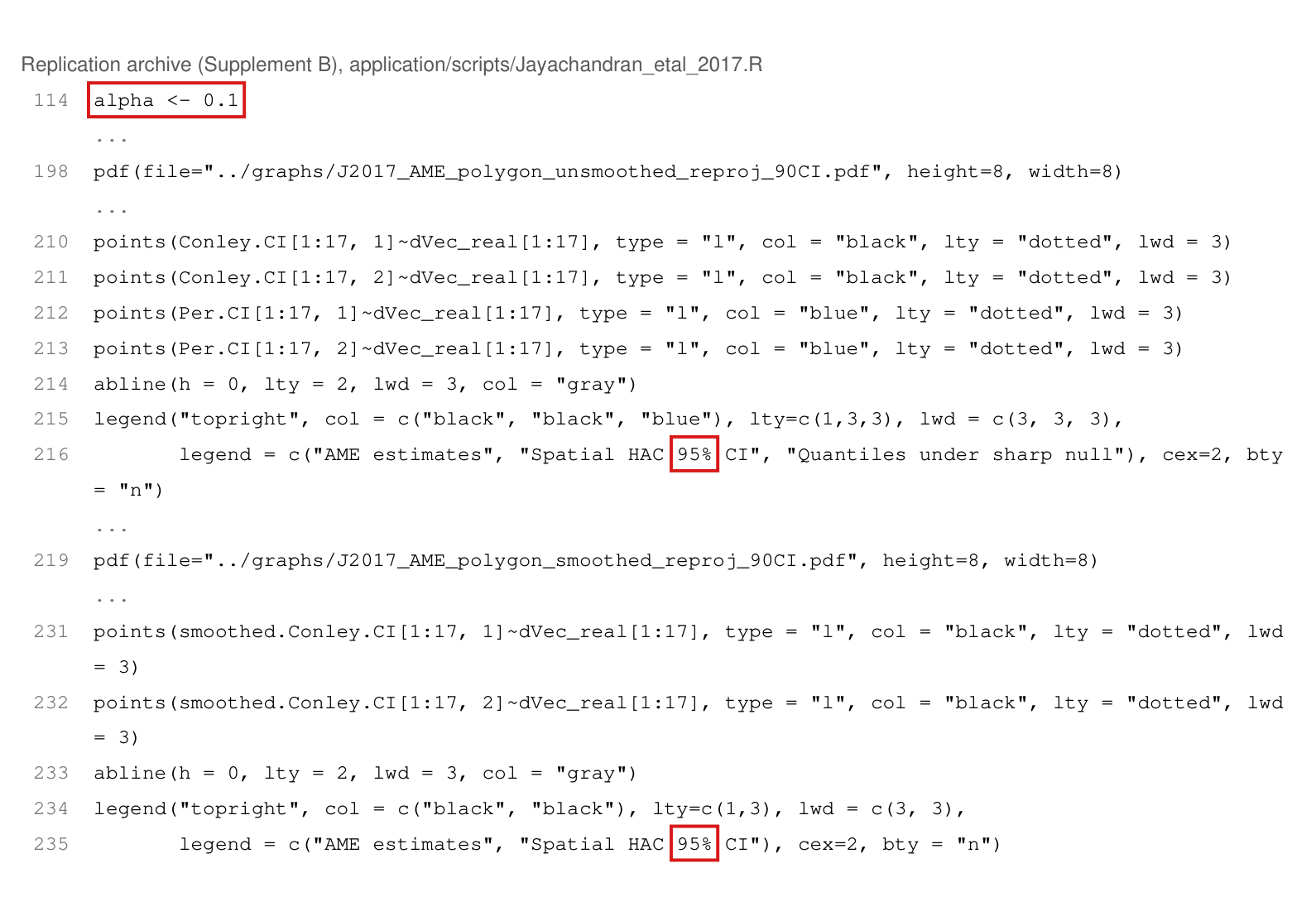
Figure 7 and Figure 8 report coverage rates and median half-lengths for the Hajek estimator with different confidence interval constructions in the additive-effect case and the interactive-effect case, respectively.
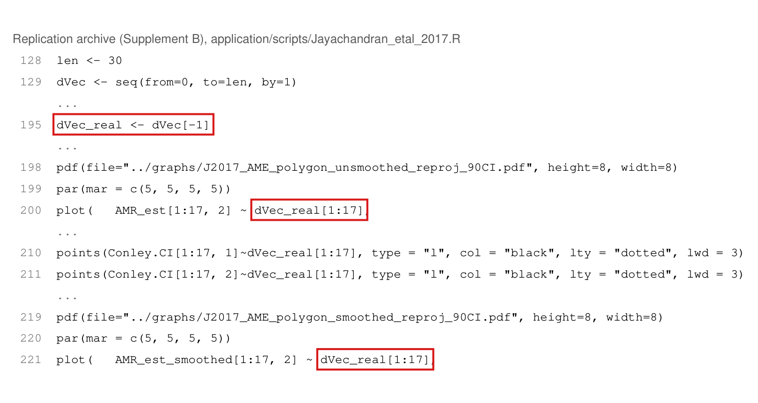
Supplement A, p. 18. We run the simulation for 2000 times. Denote the ppth assignment of Z\mathbf Z as Zp\mathbf Z_p and the value of ZiZ_i under the assignment as ZpiZ_{pi}. To obtain AME, we first calculate

τix(η)≈∑p=12000ZpiYx(Zp)∑p=12000Zpi−∑p=12000(1−Zpi)Yx(Zp)∑p=12000(1−Zpi).\tau_{ix}(\eta)\approx\frac{\sum_{p=1}^{2000}Z_{pi}Y_x(\mathbf Z_p)}{\sum_{p=1}^{2000}Z_{pi}}-\frac{\sum_{p=1}^{2000}(1-Z_{pi})Y_x(\mathbf Z_p)}{\sum_{p=1}^{2000}(1-Z_{pi})}.

Then τi(d;η)\tau_i(d;\eta) and the AME can be constructed following their definitions.

Intended meaning

The figures give Monte Carlo approximations to the mean squared error and the coverage for the fixed, design-based AME. Equation (50) states that the AME is approximated from the simulated draws, and the formula is a correct approximation: under independent Bernoulli assignment, τix\tau_{ix} is the difference of the conditional means of Yx(Z)Y_x(\mathbf Z) given Zi=1Z_i=1 and given Zi=0Z_i=0, and (50) is the difference of the corresponding sample means. Nothing printed is false.

What the text leaves out is that the replication code computes this benchmark from the same outcomes and assignments on which the estimator is then evaluated. Let BB be the benchmark, θ\theta the AME, δ=B−θ\delta=B-\theta, and eˉ\bar e the mean error of the estimates over the draws. Expanding the square, I find that the mean squared error computed against BB minus the one computed against θ\theta equals δ2−2δeˉ\delta^2-2\delta\bar e in every run. In a constructed example with 64 nodes and 2000 draws, the mean squared error is 4 against the AME and 3 against the benchmark, and an interval of half-width 1 covers the AME in no draw and the benchmark in three quarters of the draws. This example is not the design of the paper. The simulation outputs are not in the replication archive, and neither the size nor the sign of any effect on the published curves is known. The half-lengths of the intervals do not depend on the benchmark.

Corrected

Add after (50): The mean squared errors and coverage rates reported below are computed relative to this approximation of the AME, which is obtained from the same 2000 draws. The error of the approximation is not assessed separately.

The approximation can be avoided, since both designs have a closed form. Under (47), τix(η)=fx(dix)\tau_{ix}(\eta)=f_x(d_{ix}). Under (49) with assignment probability 1/21/2,

τix(η)=fx(dix)+12 gx(dix)+12∑j: N(j)=igx(djx).\tau_{ix}(\eta)=f_x(d_{ix})+\tfrac12\,g_x(d_{ix})+\tfrac12\sum_{j:\,\mathcal N(j)=i}g_x(d_{jx}).
Crop of seven lines of text. They read: Figure 6 shows the mean squared errors of the Hajek estimator for both additive-effect (31) and interactive-effect cases (32), with intervention-node sample sizes of 64, 100, and 144. In both cases the MSEs decrease as sample sizes increase, as predicted by our theory. Figure 7 and Figure 8 report coverage rates and median half-lengths for the Hajek estimator with different confidence interval constructions in the additive-effect case and the interactive-effect case, respectively. For brevity, we only display the case with a sample size of 144. The results are illustrated for AMEs at different distance values. Red outlines surround the words the mean squared errors of the Hajek estimator and the words coverage rates.
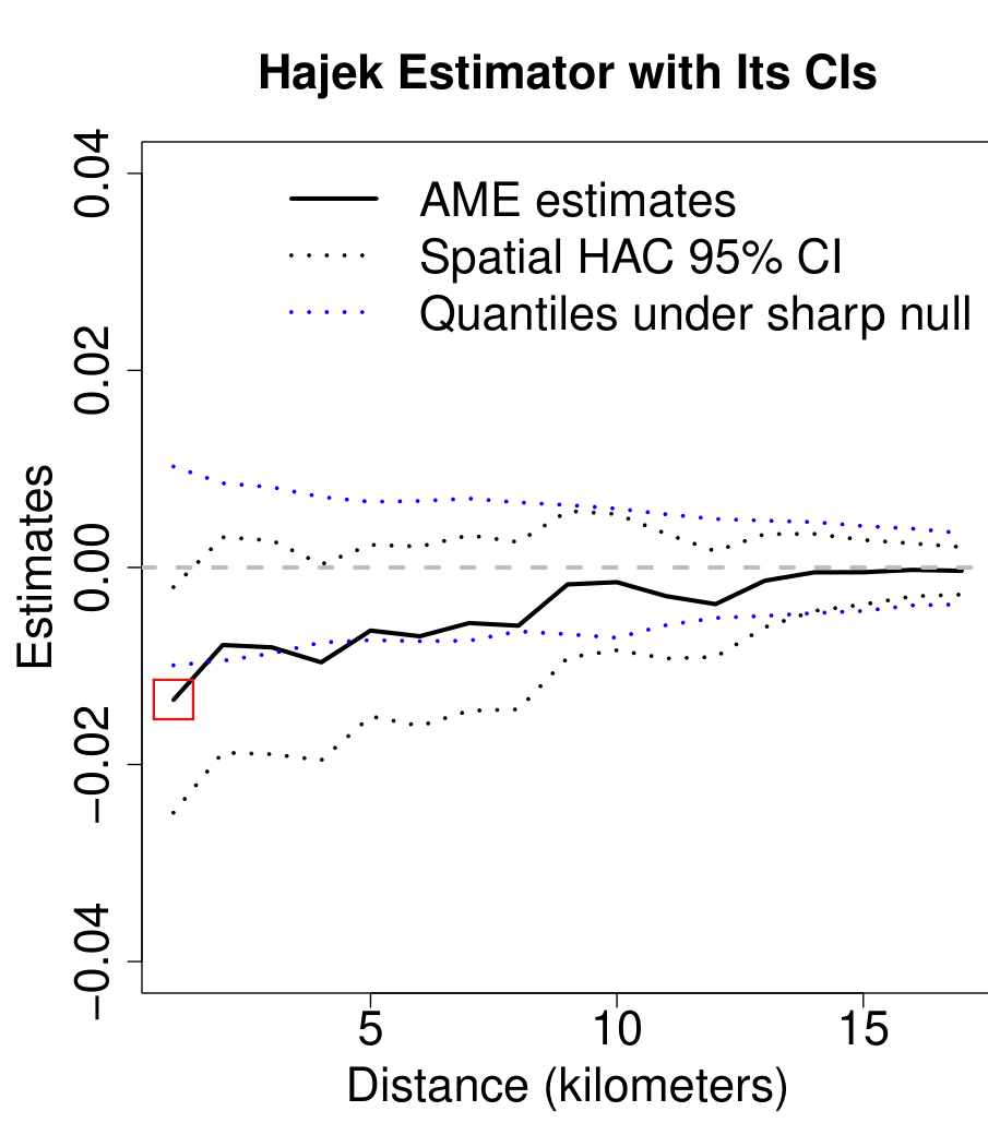
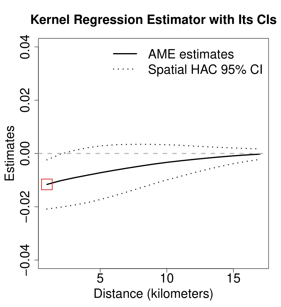
Section 7, p. 760 (PDF p. 17). The outlines mark the two quantities that are computed against the approximated AME.
Crop of three lines of text, equation (50) and one more line. The text reads: For our simulation, we use a Bernoulli design where Z sub i equals 1 with probability 0.5 for all intervention nodes. We run the simulation for 2000 times. Denote the pth assignment of Z as Z sub p and the value of Z sub i under the assignment as Z sub pi. To obtain AME, we first calculate. Equation (50) gives tau sub ix of eta as approximately the ratio of the sum over p from 1 to 2000 of Z sub pi times Y sub x of Z sub p to the sum of Z sub pi, minus the same ratio with 1 minus Z sub pi. The last line reads: Then tau sub i of d and eta and the AME can be constructed following their definitions. One red outline surrounds the words To obtain AME, we first calculate, and another surrounds the equation.
Supplement A, Appendix B.1, p. 18. The outlines mark the sentence that introduces the approximation and equation (50).

In Section 8 and in the legends of Figures 11 and 13, d~\tilde{d} and “cutoff” denote the assumed range of interference, not the cutoff of the HAC kernel that Section 5 calls d~\tilde{d}; the kernel cutoff used at distance dd is twice the stated value plus 2d2d.

Section 8.1, p. 763 (PDF p. 20), and footnote 25; Section 5, p. 755 (PDF p. 12), after equation (19); legends of Figures 11 and 13, pp. 764–765

As printed

Section 5, p. 755: “d~\tilde{d} is a cutoff value, and our setup suggests setting it at d~=h(d)\tilde{d}=h(d).”

Section 8.1, p. 763: “we assess the robustness of inferences by considering a range of cutoff values (d~\tilde{d} = 2 km, 5 km and 10 km).”

Footnote 25: “To be precise, for AME at distance value d, we set the bandwidth at 2d~+2d2\tilde{d}+2d, as discussed in Section 4.”

Legends of Figures 11 and 13: cutoff=2km, cutoff=5km, cutoff=10km.

Intended meaning

Footnote 25 settles the meaning. The values 2, 5 and 10 km are assumed ranges of interference, the quantity written dˉ\bar{d} in Section 4, where h(d)h(d) is set to 2dˉ+2d2\bar{d}+2d. The kernel cutoff of (19) at distance dd is then 4+2d4+2d, 10+2d10+2d or 20+2d20+2d km. The application script in the replication archive computes its kernel cutoff in the same way, which supports this reading. No bandwidth or interval is wrong because of the notation.

Corrected

Section 8.1: “we assess the robustness of inferences by considering a range of assumed ranges of interference (dˉ\bar{d} = 2 km, 5 km and 10 km).”

Footnote 25: “To be precise, for AME at distance value dd, we set the kernel cutoff at d~=2dˉ+2d\tilde{d}=2\bar{d}+2d, as discussed in Section 4.”

In the legends and captions of Figures 11 and 13, and in the sentence of Section 8.2 that sets the cutoff value, write “assumed interference range” in place of “cutoff”.

Five lines of body text. A red box marks the words: cutoff values (d-tilde = 2 km, 5 km and 10 km). A footnote mark 25 follows the parenthesis.
Section 8.1, p. 763 (PDF p. 20): the values 2, 5 and 10 km are introduced as cutoff values and written d~\tilde{d}.
Footnotes 24 and 25. In footnote 25 a red box marks the words: bandwidth at 2 d-tilde + 2d.
Footnote 25, p. 763 (PDF p. 20): the bandwidth actually used is 2d~+2d2\tilde{d}+2d.
Three lines of body text. A red box marks the sentence: d-tilde is a cutoff value, and our setup suggests setting it at d-tilde = h(d).
Section 5, p. 755 (PDF p. 12), after equation (19): d~\tilde{d} is defined as the cutoff of the kernel, with the suggested value h(d)h(d).

Supplement A reuses the labels C1–C6 for different assumptions: in A.6, “C 1” and “C 2” are a logistic-model block and a homophily condition, and in Appendix C, “C 3”–“C 6” are four new conditions.

Supplement A, A.6, pp. 13–16, and Appendix C, pp. 26–35 (the same supplement PDF pages)

As printed

A.6, p. 13: “C 1. The following properties hold for all sample size NN and for all i∈SNi\in\mathcal S_N: …”; p. 14: “C 2. For all sample size NN, …”; Proposition 4, pp. 15–16: “Under C2, C3, C4, C6, and C1, …” and “In addition under C2, …”.

Appendix C, p. 26: “We shall inherit C1 and C2. We relax C3 with the following weak-dependence assumption. C 3. …”; p. 27: “C 4. …”; p. 32: “C 5. The kernel function …”; p. 34: “The following assumption is similar as C5. C 6. …”, with footnote 20: “Note if bNb_N is fixed and KK is the uniform kernel, this reduces to C5.”; Proposition 6, p. 35: “Under C1, C2, C3, C4, C5 and C6”.

Intended meaning

In A.6, C6 is the article’s assignment condition and “C 1” is the new block of conditions on the logistic model. In Proposition 4 the first “C2” is the article’s bounded outcomes: the proof on p. 16 uses it, with bounded confounders, to control remainders. The “C2” of “In addition under C2” and of item (ii) is the homophily condition of p. 14. Appendix C states that it keeps C1 and C2 of the article and replaces C3. Its “C 3”–“C 6” are local conditions (near-epoch dependence, a quadratic bound on neighborhood counts, kernel conditions and a homophily limit), and Proposition 6 uses that local set. The two comparisons on p. 34, “similar as C5” and “this reduces to C5”, refer to the homophily condition C5 of the article, not to the kernel condition labeled “C 5” on p. 32. With these readings the hypotheses of the supplement’s propositions are recoverable, and no result depends on the labels.

Corrected

Give the two conditions of A.6 the labels O1 (logistic model) and O2 (homophily), and state Proposition 4 as “Under C2, C3, C4, C6, and O1, … In addition under O2, …”. Give the conditions of Appendix C the labels W3–W6, and state its results under “C1, C2, W3, W4, W5 and W6”. On p. 34, write “similar to C5 of the article” and “this reduces to C5 of the article”.

Crop of the heading 'A.6. Theoretical Results on Observational Studies', its introductory paragraph, and the line 'C 1. The following properties hold for all sample size N and for all i in S_N:' followed by item (i). A red box marks the label 'C 1.'
Supplement A, p. 13, the start of A.6. The marked label “C 1.” names a new block of conditions on the logistic assignment model; C1 of the article is the Bernoulli design.
Crop of the line 'Under C2, C3, C4, C6, and C1,' and of equation (36), which states that the linearized and the fitted IPW estimators differ by o_p(N to the power minus one half). Red boxes mark 'C2' and 'C1'.
Supplement A, p. 15, Proposition 4 of A.6, the hypothesis of (36). The marked “C2” is the article’s bounded-outcomes condition and the marked “C1” is the logistic block of p. 13.
Crop of the line 'In addition under C2,' and the first line of the displayed upper bound on the variance of the linearized IPW estimator. A red box marks 'C2'.
Supplement A, p. 16, the continuation of Proposition 4. The marked “C2” is the homophily condition of p. 14, not the condition of the same name on p. 15.
Crop of the sentence 'The following assumption is similar as C5.', the line 'C 6. Given a kernel function K and a sequence of bandwidth b_N,' and equation (122), a liminf condition on a kernel-weighted sum of products of centered node effects. Red boxes mark 'C5' and the label 'C 6.'
Supplement A, p. 34, Appendix C. The marked “C5” refers to the homophily condition of the article; the marked “C 6.” is a new condition local to Appendix C.

Proposition 4 states that the coverage probabilities of the two intervals have limits of at least 1−α1-\alpha; under its conditions the limits need not exist, and the guarantee to read is that their limits inferior are at least 1−α1-\alpha.

Proposition 4, p. 755 (PDF p. 12)

See also under Formal statements (Lean): P004-T43

As printed

Proposition 4, p. 755: “Let K(⋅)K(\cdot) in (19) be the uniform kernel. Under C1–C4 and if N×AVar⁡(τ^HA(d))N\times\operatorname{AVar}(\widehat\tau_{\mathrm{HA}}(d)) is uniformly bounded below for all large NN, […] for each α<1\alpha<1:

(i) lim⁡N→∞Prob(zα2≤τ^HA(d)−AME(d;η)V^SAH(d)≤z1−α2)≥1−α;\text{(i) }\colorbox{#ffe58a}{$\displaystyle \lim_{N\to\infty}$}\mathrm{Prob}\Biggl(z_{\frac\alpha2}\le\frac{\widehat\tau_{\mathrm{HA}}(d)-\mathrm{AME}(d;\eta)}{\sqrt{\widehat{\mathrm V}_{\mathrm{SAH}}(d)}}\le z_{1-\frac\alpha2}\Biggr)\ge1-\alpha;
(ii) additionally under C5, lim⁡N→∞Prob(zα2≤τ^HA(d)−AME(d;η)V^HAC(d)≤z1−α2)≥1−α.”\text{(ii) additionally under C5, }\colorbox{#ffe58a}{$\displaystyle \lim_{N\to\infty}$}\mathrm{Prob}\Biggl(z_{\frac\alpha2}\le\frac{\widehat\tau_{\mathrm{HA}}(d)-\mathrm{AME}(d;\eta)}{\sqrt{\widehat{\mathrm V}_{\mathrm{HAC}}(d)}}\le z_{1-\frac\alpha2}\Biggr)\ge1-\alpha.\text{''}

Intended meaning

The conditions of Proposition 4 bound the coverage probabilities from below as NN grows, but they do not make them converge. In a design that satisfies C1–C4 and the variance bound, with units spaced so that each forms its own neighbourhood, treatment probability 1/21/2 and bounded outcomes whose form differs between even and odd NN, the coverage of the interval in part (i) at α=1/2\alpha=1/2 tends to 1/21/2 along even NN and to about 0.660.66 along odd NN, so it has no limit. Both values are at least 1−α1-\alpha, and the interval does not cover too rarely. Read as the statement that the limit inferior of each coverage probability is at least 1−α1-\alpha, which is what an asymptotically conservative interval requires, the proposition is not affected by the example. The example concerns part (i); part (ii) asserts a limit of the same form.

Corrected

Proposition 4, restated: let K(⋅)K(\cdot) in (19) be the uniform kernel. Under C1–C4, and if N×AVar⁡(τ^HA(d))N\times\operatorname{AVar}(\widehat\tau_{\mathrm{HA}}(d)) is bounded below by a positive constant for all large NN, then for each 0<α<10<\alpha<1:

(i) lim inf⁡N→∞Prob(zα2≤τ^HA(d)−AME(d;η)V^SAH(d)≤z1−α2)≥1−α;\text{(i) }\colorbox{#ffe58a}{$\displaystyle \liminf_{N\to\infty}$}\mathrm{Prob}\Biggl(z_{\frac\alpha2}\le\frac{\widehat\tau_{\mathrm{HA}}(d)-\mathrm{AME}(d;\eta)}{\sqrt{\widehat{\mathrm V}_{\mathrm{SAH}}(d)}}\le z_{1-\frac\alpha2}\Biggr)\ge1-\alpha;
(ii) additionally under C5, lim inf⁡N→∞Prob(zα2≤τ^HA(d)−AME(d;η)V^HAC(d)≤z1−α2)≥1−α.\text{(ii) additionally under C5, }\colorbox{#ffe58a}{$\displaystyle \liminf_{N\to\infty}$}\mathrm{Prob}\Biggl(z_{\frac\alpha2}\le\frac{\widehat\tau_{\mathrm{HA}}(d)-\mathrm{AME}(d;\eta)}{\sqrt{\widehat{\mathrm V}_{\mathrm{HAC}}(d)}}\le z_{1-\frac\alpha2}\Biggr)\ge1-\alpha.
Crop of Proposition 4 and its two displays. Red boxes surround lim and its subscript N at the start of part (i) and of part (ii); the arrow and infinity sign of each subscript lie just outside the boxes.
Proposition 4, p. 755 (PDF p. 12): both parts state an ordinary limit.

Formal statements (Lean)

Formal results: 33 whole; 6 restricted; 0 refuted; 4 omitted.

Coverage concerns the identified claim under its stated assumptions. A checked proof establishes the formal statement; correspondence to the published text was reviewed by AI. Repository access is currently required to open the source links.

Each result links to its current formal statement and proof. “Whole” covers the identified claim under its assumptions; “restricted” covers the stated narrower scope; “refuted” gives a counterexample to the identified assertion; “omitted” has no current theorem. Any named published theorem used as a premise remains an assumption. Browse the formal results for this work.

Supplement A, Appendix A.6, Proposition 4, equation (36): the linearization of the IPW estimator with estimated logistic propensity scores. A design satisfying every stated hypothesis in which N(τ^IPWL(d)−τ^IPW(d))\sqrt N(\hat\tau^{\mathrm L}_{\mathrm{IPW}}(d)-\hat\tau_{\mathrm{IPW}}(d)) does not tend to zero in probability

Supplement A p. 15 (Proposition 4, eq. (36)); pp. 16-17 (proof: eqs. (42)-(43) and the display 'Hence (42) becomes'); definitions on Supplement A pp. 13-14; advertised in the article, Section 6.4, p. 759 (PDF p. 16)

Supplement A pp. 13-17, Proposition 4, eqs. (36), (42)-(43). The printed claim is false: the balanced three-type spatial design satisfies every stated hypothesis, with the displayed exact information, coefficients, effects and variance constants. Its independent blocks have the stated exact second and fourth moments and the positive uniform tail bound. An actual constrained logistic MLE has the corrected order-N⁻¹ expansion, so the printed root-N remainder fails to converge to zero. The fitted estimator's Gaussian variance is 3/625, its printed-variance standardization has limiting variance 3600/1753, and intervals consistent for the printed variance have the stated strict coverage deficit for every 0<α<1.

Historical component credits

Supplement A, Appendix A.6, Proposition 4, corrected: first-order expansion of the IPW estimator with an estimated logistic propensity score, its variance, and the HAC and SAH variance bounds built on the corrected residuals

Supplement A pp. 14-17 (Appendix A.6: 'C 2', Proposition 4, eqs. (36)-(43)); article Section 6.4, p. 759 (PDF p. 16)

Supplement A pp. 14-17 (Appendix A.6: 'C 2', Proposition 4, eqs. (36)-(43)); article Section 6.4, p. 759 (PDF p. 16). The corrected IPW estimator has the expansion, exact representations, unbiasedness, variance formula, oracle bounds, normal limit and conservative intervals in clauses (a)-(e). The usual measure-theoretic conditions are assumed.

Historical component credits
  • Proved AronowAudit.P004.corrected_fits Historical support retained; baseline fidelity: ok; manifest: used; used in Solution; Fidelity sweep: ok
  • Proved AronowAudit.P004.corrected_score_identity Historical support retained; baseline fidelity: ok; manifest: used; used in Solution; The summand identity is used inside corrected_ipw_finite, which supplies the exact estimator representation.
  • Proved AronowAudit.P004.corrected_ipw_finite Historical support retained; baseline fidelity: ok; manifest: used; used in Solution; These finite identities remain valid as algebraic statements in singular or empty dimensions; this adds cases and does not exclude the nonsingular logistic specialization the claim needs.
  • Proved AronowAudit.P004.residualContrast_mean Historical support retained; baseline fidelity: ok; manifest: used; used in Solution; The corrected residual mean is already supplied by corrected_ipw_finite.
  • Proved AronowAudit.P004.augmented_unbiased Historical support retained; baseline fidelity: ok; manifest: used; used in Solution; Unbiasedness is already supplied by corrected_ipw_finite; this helper is not separately invoked.
  • Proved AronowAudit.P004.augmented_variance Historical support retained; baseline fidelity: ok; manifest: used; used in Solution; Fidelity sweep: ok
  • Proved AronowAudit.P004.corrected_ipw_oracle Historical support retained; baseline fidelity: ok; manifest: used; used in Solution; Fidelity sweep: ok
  • Proved AronowAudit.P004.Wave1.corrected_ipw_asymptotics_proof Historical support retained; baseline fidelity: ok; manifest: used; used in Solution; The credited component is the corrected T2(a,e), whose text already requires interior truth, corrected score fits, liminf coverage, and HAC truncation; these are not extra restrictions relative to that component. No conclusion is hidden in a hypothesis.

Supplement A, Appendix A.6: the observational SAH variance estimator V^SAHobs(d)\hat V^{\mathrm{obs}}_{\mathrm{SAH}}(d) and the coverage statement (i) of Proposition 4 built on it. A design in which NV^SAHobsN\hat V^{\mathrm{obs}}_{\mathrm{SAH}} converges to 825\frac8{25} of N Var(τ^IPW)N\,\mathrm{Var}(\hat\tau_{\mathrm{IPW}})

Supplement A p. 15 (definitions of ϵ^i\hat\epsilon_i and V^SAHobs(d)\hat V^{\mathrm{obs}}_{\mathrm{SAH}}(d)); p. 16 (Proposition 4, item (i))

Supplement A pp. 15-16, observational residual, SAH variance and Proposition 4(i). The printed claim is false: the specified N=8r two-group disk field and actual clipped logistic MLE satisfy the stated assumptions, with singleton neighborhoods and zero AME. The exact fitted estimator, coefficients, residual sum and double-weighted variance have the stated formulas. The N=32 and N=64 variances and expectations give the stated strict finite underestimation. The root-N Gaussian variance and scaled actual variance tend to 1/4, the pooled treatment fraction N₁/N and normalized residual sum R/N tend in probability to 1/5 and 1/8, and the printed scaled variance and variance ratio tend to 2/25 and 8/25. Every 0<α<1/2 has the stated exact limiting coverage strictly below 1-α.

Historical component credits
  • Proved AronowAudit.P004.Wave1.observational_sah_counterexample_proof Historical support retained; baseline fidelity: ok; manifest: not used; not used in Solution; The row covers the actual-MLE variance-ratio witness, not the target's additional finite tables, normal limit, or all-alpha coverage formula. The alternative realization satisfies every hypothesis of the printed reading, so it remains an exact counterexample component.
  • Proved AronowAudit.P004.sah_witness_constants Historical support retained; baseline fidelity: ok; manifest: not used; not used in Solution; Entered rational comparisons do not identify the actual estimator expectations or variances.

Supplement A, Appendix A.6: the observational SAH variance estimator, corrected so that each residual is weighted by the inverse propensity once

Supplement A p. 15 (definitions of ϵ^i\hat\epsilon_i and V^SAHobs(d)\hat V^{\mathrm{obs}}_{\mathrm{SAH}}(d))

Supplement A p. 15, definitions of the observational residual and SAH variance. Use raw fitted residuals with squared inverse propensities. With both arms nonempty this has the stated equivalent arm-count form; the printed weighted residual instead produces fourth powers. Under independent assignment, symmetric self-containing neighborhoods and zero covariance outside them, the variance of the residual contrast mean is bounded by the stated conditional second moments, exactly the expectation of the raw SAH estimator. In the T3 design its N-scaled limit is 1/2, compared with actual variance limit 1/4, and its N=32 expectation is exactly 493725989/38038425600, above 18239/1505280. General fitted-IPW intervals use the residuals of the corrected linearization as specified in T2.

Historical component credits
  • Proved AronowAudit.P004.sah_weighting_identity Historical support retained; baseline fidelity: ok; manifest: used; used in Solution; The modelling-choice sentence about a finite variance bound and symmetry describes the accompanying T4(b) result; this row itself is only the pointwise T4(a) identity and needs no neighborhood restrictions.
  • Proved AronowAudit.P004.raw_sah_bound Historical support retained; baseline fidelity: ok; manifest: used; used in Solution; Fidelity sweep: ok

Section 8.1, the reading of the summed Hajek estimates between zero and five km as 'a 3.4 percentage point decline in deforested area': binary-outcome designs with the same sum −0.034-0.034 and area-average effects −173000-\frac{17}{3000}, +12118000+\frac{121}{18000} and −71800-\frac7{1800}

p. 763 (PDF p. 20), last paragraph, continued on p. 764 (PDF p. 21); definitions: eq. (2), p. 747; eqs. (8)-(9), p. 750; eq. (16), p. 754

pp. 763-764 (PDF pp. 20-21), interpretation of the sum of point Hajek estimates; eqs. (2), (8)-(9), (16). These examples refute the reading that an unweighted sum of point Hajek contrasts over a partition equals the change in the normalized deforested area share of the union. Three specified binary area fields on the two radius-one disk nodes realize Cases A, B and C. All six bin areas, positive finite averages, all-assignment shares and whole-region weighted averages have the stated values. At assignment (1,0), each bin Hajek contrast is its AME and each six-bin sum is -17/500; the actual whole-region contrasts and AMEs are -17/3000, 121/18000 and -7/1800. Case B reverses the sign and Case C's sum is below every bin effect. Refining the same Case A field into eleven bins changes the sum to -187/3000 while preserving its whole-region effect -17/3000. No corrected empirical area effect is asserted for the application.

Historical component credits
  • Proved AronowAudit.P004.Wave1.spatial_area_sum_counterexample_proof Historical support retained; baseline fidelity: ok; manifest: not used; not used in Solution; This duplicate projection is contained in the stronger all-assignment spatial Case B row.
  • Proved AronowAudit.P004.Wave1.area_sum_counterexample_proof Historical support retained; baseline fidelity: ok; manifest: not used; not used in Solution; This projection is contained in the stronger all-assignment spatial Case B row.
  • Proved AronowAudit.P004.area_witness_realized Historical support retained; baseline fidelity: ok; manifest: not used; not used in Solution; Finite-table arithmetic is subsumed by the actual spatial Case B row.
  • Proved AronowAudit.P004.assignment_two_univ Historical support retained; baseline fidelity: ok; manifest: not used; not used in Solution; The all-assignment spatial row already supplies the required design witness; assignment enumeration is not separately invoked.
  • Proved AronowAudit.P004.Wave1.area_sum_spatial_caseB Historical support retained; baseline fidelity: ok; manifest: not used; not used in Solution; The statement exports the all-assignment equality and exact partition, as well as the area-integral sign reversal; selecting Case B is the stated component, not an undisclosed restriction on a universal positive theorem.

Section 8.1, corrected: the summed distance-specific estimates are a summed contrast; the area-average effect is the area-weighted mean of the bin effects; the randomization p-value does not depend on the scaling of the statistic

p. 763 (PDF p. 20), last paragraph, continued on p. 764 (PDF p. 21)

p. 763 (PDF p. 20), last paragraph, continued on p. 764 (PDF p. 21). Actual area averages and their marginalized effects aggregate with bin masses, lie within bin bounds, and positive scaling preserves randomization p-values.

Historical component credits
  • Proved AronowAudit.P004.area_partition_identity Historical support retained; baseline fidelity: ok; manifest: used; used in Solution; Auxiliary realized-average identity; item 02 supplies the effect aggregation. The regularity assumptions are the ordinary meaning of the finite-mass averages in the claim, rather than a separate statistical restriction.
  • Proved AronowAudit.P004.weighted_effect_bounds Historical support retained; baseline fidelity: ok; manifest: used; used in Solution; Fidelity sweep: ok
  • Proved AronowAudit.P004.marginal_bin_average Historical support retained; baseline fidelity: ok; manifest: used; used in Solution; {'source': 'adjudication', 'decision': 'rejected', 'what': "P004_Spatial.lean:2582 states that the bin-mass average commutes with each arm-specific marginal mean, for arbitrary node-specific weights. Applying it to both arms and subtracting gives exactly T6(a)'s node-effect aggregation, since nodeEffect is their difference (P004_Spatial.lean:75); the explicit corollary is also stated at line 2605. Thus no positive-mass bin configuration or effect conclusion is lost, and the extra signed-weight and zero-denominator cases do not restrict the claim. The description should identify the directly stated arm-mean identity rather than call this declaration the explicit effect identity."}
  • Proved AronowAudit.P004.bin_effect_aggregation Historical support retained; baseline fidelity: ok; manifest: used; used in Solution; Fidelity sweep: ok
  • Proved AronowAudit.P004.randomization_scaling Historical support retained; baseline fidelity: ok; manifest: used; used in Solution; Fidelity sweep: ok

Section 7 recommendation ('the positive semidefinite HAC variance estimator with the empirical degree of adjustment') read with Supplement A.7: a design satisfying C1-C5 in which the adjusted positive-semidefinite variance converges to 1516\frac{15}{16} of the asymptotic variance, and an assignment in which the adjusted ordering is reversed

p. 761 (PDF p. 18), Section 7; p. 756 (PDF p. 13), eqs. (21)-(22) and footnotes 14-15; Supplement A p. 17 (A.7, eqs. (44)-(45))

p. 761 (PDF p. 18), Section 7; p. 756 (PDF p. 13), eqs. (21)-(22) and footnotes 14-15; Supplement A p. 17 (A.7, eqs. (44)-(45)). The repeated-star construction gives a finite adjustment-order reversal and a guarded asymptotic coverage upper bound strictly below 95 percent.

Historical component credits
  • Counterexample proved AronowAudit.P004.adjusted_pd_finite_counterexample Historical support retained; baseline fidelity: ok; manifest: used; used in Solution; The finite row covers Witness 2 only. The original modelling paragraph mentions Student density/quantiles in the wider witness setup, but those occur in the separate asymptotic row, not this finite conclusion. The recorded review note about an unproved source and sorryAx is stale relative to this task's stipulated standard-axiom proofs; proof status is outside this fidelity audit.
  • Proved AronowAudit.P004.Wave1.adjusted_pd_asymptotic_counterexample_proof Historical support retained; baseline fidelity: ok; manifest: used; used in Solution; The target fixes the adjusted-procedure interpretation and the 95-percent repeated-star witness. Direct Student-interval undercoverage is exported, not merely an underestimated scalar variance; the concrete Q=K+vv^T/8 is the genuine positive part since Kv=-v and ||v||^2=8.
  • Proved AronowAudit.P004.adjusted_pd_constants Historical support retained; baseline fidelity: ok; manifest: used; used in Solution; Fidelity sweep: ok

Section 7 recommendation and Supplement A.7, corrected: an adjustment of the positive-semidefinite HAC variance that cannot reduce it, and the guarantee it inherits from Proposition 4(ii)

p. 761 (PDF p. 18), Section 7; p. 756 (PDF p. 13), eqs. (21)-(22), footnote 15; Supplement A p. 17 (A.7)

p. 761 (PDF p. 18), Section 7; p. 756 (PDF p. 13), eqs. (21)-(22), footnote 15; Supplement A p. 17 (A.7). Capping the positive-semidefinite HAC adjustment preserves variance ordering and interval inclusion for every symmetric kernel. Every positive-degree Student upper quantile dominates the normal quantile. Under C1-C5 and the variance floor, the capped intervals have asymptotic coverage at least one minus alpha, including arbitrary assignment-dependent positive Student degrees of freedom. Coverage counts only draws with both arms nonempty. The repeated-star design has well-defined uncapped intervals with probability tending to one and shows that the uncapped rule has no such universal guarantee.

Historical component credits
  • Proved AronowAudit.P004.capped_variance_ge Historical support retained; baseline fidelity: ok; manifest: used; used in Solution; The scalar cap inequality is incorporated in capped_pd_interval.
  • Proved AronowAudit.P004.capped_pd_interval Historical support retained; baseline fidelity: ok; manifest: used; used in Solution; Fidelity sweep: ok
  • Proved AronowAudit.P004.Wave1.capped_pd_coverage_proof Historical support retained; baseline fidelity: ok; manifest: used; used in Solution; This is exactly the corrected liminf claim, including arbitrary random critical values satisfying the stated lower bound. The hypotheses do not assume a CLT, variance consistency, positive adjusted trace, or the desired coverage conclusion.

Supplement A, Appendix A.6, Lemma A.6 (score expansion of the logistic MLE over a compact set) with the true coefficient on the boundary of Θ0\Theta_0, as 'C 1'(iv) allows

Supplement A pp. 13-14 ('C 1' items (iv) and (vi)); p. 14 (Lemma A.6)

Supplement A pp. 13-14, C 1(iv),(vi) and Lemma A.6. The boundary-constrained one-dimensional logistic MLE over [0,1], with constant confounder one and true coefficient zero, satisfies all stated premises. Its likelihood has the stated derivatives and unique clipped-logit maximizer; its information, score remainder, exact moments and explicit finite tail lower bounds have the displayed values. The score remainder fails to be smaller than root-N. The scaled MLE converges to twice the positive part of a standard normal, while the leading score term converges to twice a standard normal. Consistency and the root-N rate hold. Thus the printed universal score expansion is false.

Historical component credits
  • Proved AronowAudit.P004.Wave1.boundary_mle_counterexample_proof Historical support retained; baseline fidelity: ok; manifest: not used; not used in Solution; The target metadata asymptotic=false conflicts with its explicit non-o_p conclusion; the row correctly derives asymptotic failure from a finite tail bound uniform over N>0. The surviving consistency and root-N rate are not refuted.

Supplement A, Appendix A.6, 'C 1'(iv) and Lemma A.6, corrected: the true logistic coefficient is an interior point of the compact parameter set

Supplement A pp. 13-14 ('C 1' item (iv)); p. 14 (Lemma A.6)

Supplement A pp. 13-14 ('C 1' item (iv)); p. 14 (Lemma A.6). Compact membership gives logistic-MLE consistency and its root-N rate, while interior truth gives the order-N^-1 and smaller-than-root-N score remainders.

Historical component credits
  • Proved AronowAudit.P004.Wave1.corrected_mle_proof Historical support retained; baseline fidelity: ok; manifest: used; used in Solution; Interiority is required only for the score expansion, exactly as corrected T10 requests. Compact membership alone supports consistency and the root-N rate; no interior or asymptotic conclusion is hidden in LogisticConditions.

Section 6.4, the observational Horvitz-Thompson estimator τ^HTobs(d)\hat\tau^{\mathrm{obs}}_{\mathrm{HT}}(d) and its unbiasedness under C6, with the control weight corrected to 1/(1−p(Oi))1/(1-p(O_i)) (also the last line of the proof in Supplement A.1.3)

p. 759 (PDF p. 16), display defining τ^HTobs(d)\hat\tau^{\mathrm{obs}}_{\mathrm{HT}}(d); Supplement A p. 4 (A.1.3, last line of the display)

p. 759 (PDF p. 16), display defining τ^HTobs(d)\hat\tau^{\mathrm{obs}}_{\mathrm{HT}}(d); Supplement A p. 4 (A.1.3, last line of the display). Corrected observational HT is unbiased, the printed estimator has the stated expectation and exact equality criterion, and the constant-outcome example has printed expectation minus two.

Historical component credits
  • Proved AronowAudit.P004.ht_unbiased Historical support retained; baseline fidelity: ok; manifest: used; used in Solution; The positivity hypothesis makes the defined conditional means equal the paper's marginalization over the other assignments. For a fixed finite N, no extra uniform-overlap restriction is needed for exact unbiasedness.
  • Proved AronowAudit.P004.printed_obs_ht_expectation Historical support retained; baseline fidelity: ok; manifest: used; used in Solution; Fidelity sweep: ok

Section 6.3, the Monte Carlo rejection rule and 'gives an α\alpha-level exact test': (A) with a negative observed statistic the printed rule never rejects; (B) the rule with absolute values on both sides, at P=100P=100 and α=120\alpha=\frac1{20}, has size 0.0555>0.050.0555>0.05 in a sharp-null Bernoulli design with eight nodes

p. 758 (PDF p. 15), Section 6.3, second paragraph

p. 758 (PDF p. 15), Section 6.3, second paragraph. The eight-node sharp-null design witnesses the signed-comparison defect and excess size of the uncorrected absolute-statistic Monte Carlo test.

Historical component credits
  • Proved AronowAudit.P004.Wave1.mc_signed_spatial_counterexample_proof Historical support retained; baseline fidelity: ok; manifest: used; used in Solution; The source comment calling eightNodeResampled one-treated is wrong: its definition treats seven nodes, giving j=127 exactly as the target requires. This is a source-comment issue, not an error in the credited original row description.
  • Proved AronowAudit.P004.Wave1.mc_level_spatial_counterexample_proof Historical support retained; baseline fidelity: ok; manifest: used; used in Solution; This proves the explicitly credited Witness B at P=100. It does not refute the assertion that a fixed finite design may become conservative for all sufficiently large P, nor does it prove Witness C at P=10000.
  • Proved AronowAudit.P004.negative_observed_comparison Historical support retained; baseline fidelity: ok; manifest: not used; not used in Solution; The retained explicit draw-array witness already demonstrates the signed-comparison defect; the separate universal assertion is not included.
  • Proved AronowAudit.P004.mc_size_counterexample Historical support retained; baseline fidelity: ok; manifest: used; used in Solution; The actual spatial rejection-size row already includes this exact size inequality.

Section 6.3, the Monte Carlo randomization test, corrected: absolute value of the observed statistic and the observed assignment counted among the draws

p. 758 (PDF p. 15), Section 6.3, second paragraph

p. 758 (PDF p. 15), Section 6.3, second paragraph. The plus-one absolute-statistic Monte Carlo test has finite-sample level, the raw rule has the stated bound, and the correction changes its p-value by the stated amount.

Historical component credits
  • Proved AronowAudit.P004.Wave1.mc_exact_level Historical support retained; baseline fidelity: ok; manifest: used; used in Solution; The current statement allows an arbitrary whole-assignment law w, so no independent-coordinate design restriction remains. Fixed sharp-null outcomes are absorbed in the arbitrary assignment statistic T. Historical repair and binding-assertion details do not change its mathematical scope.
  • Proved AronowAudit.P004.mc_plus_one_identity Historical support retained; baseline fidelity: ok; manifest: used; used in Solution; Fidelity sweep: ok

Section 6.2, the sentence after eq. (26): 'The donut and disk AMEs, defined in Section 3, are special cases with (properly-normalized) uniform kernels.' Finite designs in which the disk and donut AMEs differ from every common-kernel smoothing of the circle AMEs

p. 757 (PDF p. 14), sentence after eq. (26); definitions: eq. (2), p. 747 (PDF p. 4); eqs. (4)-(9), pp. 749-750

p. 757 (PDF p. 14), sentence after eq. (26); eq. (2), p. 747 (PDF p. 4), and eqs. (4)-(9), pp. 749-750. All three explicit Euclidean witnesses refute the printed uniform-radius disk/donut identity. The one-node atomic witness has radius effects zero and one, uniform-radius mean one half, and band effects two thirds, with shell weights one third and two thirds. The two-node witness has zero circle AMEs, band AMEs one sixth, the stated individual effects and unequal shell weights, and defeats every common pair of weights. For area on the unit disk the continuous conditional circle-effect version is radius itself; radial area has density 2r/(b squared minus a squared). Disk averages are two thirds versus one half, and annulus averages seven ninths versus three quarters. Every atomic and positive-area band average exists; singleton area circles are conditional means.

Historical component credits
  • Counterexample proved AronowAudit.P004.spatial_shell_counterexample Historical support retained; baseline fidelity: ok; manifest: used; used in Solution; The record's review note says the source remains unproved, conflicting with the supplied counterexample_proved status and the task's compilation premise; this is stale proof-status metadata, not a statement defect.
  • Counterexample proved AronowAudit.P004.shell_counterexample Historical support retained; baseline fidelity: ok; manifest: not used; not used in Solution; The two names have the same exact spatial Witness 2 statement; only spatial_shell_counterexample is invoked.

Section 6.2, the sentence on donut and disk AMEs, corrected: they are shell-mass-weighted, node-specific averages of the circle effects

p. 757 (PDF p. 14), sentence after eq. (26)

p. 757 (PDF p. 14), sentence after eq. (26); eqs. (2), (7)-(9). Band effects average marginalized point effects using node-specific shell masses. Continuous circle effects are signed pushforward densities, with the actual shell means at positive atoms. Finite shell decompositions and their node mean hold without common weights; common weights give a weighted sum of circle AMEs. A common kernel works for every bounded measurable profile if and only if all normalized node measures equal it. Circle AMEs alone do not determine the band AME. Full planar annuli have density 2r/(b²-a²), including disks at a=0, and their radial measure differs from the uniform radial measure. The usual measure-theoretic conditions are assumed.

Historical component credits
  • Proved AronowAudit.P004.band_effect_identity Historical support retained; baseline fidelity: ok; manifest: not used; not used in Solution; The required component is T15(a); neither a common radial kernel nor planar area weighting is assumed.
  • Proved AronowAudit.P004.Wave1.supported_shell_identity Historical support retained; baseline fidelity: ok; manifest: used; used in Solution; No claim-stage verdict change. This duplicates R032-04 under a different name; arbitrary node-specific band totals and supports are retained and the common weights are only required for clause (c).
  • Proved AronowAudit.P004.Wave1.shell_mass_identity Historical support retained; baseline fidelity: ok; manifest: not used; not used in Solution; This is a duplicate of supported_shell_identity with the same node-specific contract.
  • Proved AronowAudit.P004.Wave1.annulus_radial_measure_proof Historical support retained; baseline fidelity: ok; manifest: used; used in Solution; This row covers T15(d), including a=0; the correction to the printed uniform density is the target itself, not a fidelity difference.

Section 4, the two sufficient conditions offered for C3 and C4, for polygon intervention nodes: (A) effects confined to within dˉ\bar d of their source do not give h(d)=2dˉ+2dh(d)=2\bar d+2d; (B) a lower bound on polygon area does not give C4

p. 752 (PDF p. 9), paragraph 'For an interpretable sufficient condition ...'; p. 753 (PDF p. 10), sentence on polygon-intervention experiments after C4; footnote 25, p. 763 (PDF p. 20)

p. 752 (PDF p. 9), paragraph 'For an interpretable sufficient condition ...'; p. 753 (PDF p. 10), polygon-intervention spacing sentence; footnote 25, p. 763. The zero-radius rectangle witness, every prescribed separation L>5, and the positive-radius two-atom witness refute the range-only cutoff, with exact distances, averages, interference indicators and covariance. Disjoint area-one thin polygons have the stated exact squared distances and an unbounded radius-two neighborhood count, refuting area-only spacing.

Historical component credits
  • Proved AronowAudit.P004.Wave1.polygon_range_counterexample_proof Historical support retained; baseline fidelity: ok; manifest: used; used in Solution; This row is a witness for the sufficient-condition failure, not a refutation of propositions assuming C3. The positive-distance alternative witness is unnecessary for this refutation.
  • Proved AronowAudit.P004.Wave1.no_polygon_cutoff_from_range_alone_proof Historical support retained; baseline fidelity: ok; manifest: used; used in Solution; This is the full arbitrary-h witness family for A4, not a claim that a fixed finite population has no possible cutoff. Status proved is consistent with proving a counterexample conjunction.
  • Proved AronowAudit.P004.Wave1.polygon_spacing_counterexample_proof Historical support retained; baseline fidelity: ok; manifest: used; used in Solution; The printed positive area threshold can be any fixed value below 1. The weaker exported distance estimate still refutes C4, so it loses none of the intended counterexample conclusion.

Section 4, the sufficient conditions for C3 and C4, corrected: h(d)=2dˉ+2dh(d)=2\bar d+2d for point nodes, 2dˉ+2d+D2\bar d+2d+D for nodes of diameter at most DD; and a neighbourhood-count bound from disjoint interiors, an area lower bound and a diameter upper bound

p. 752 (PDF p. 9), paragraph 'For an interpretable sufficient condition ...'; p. 753 (PDF p. 10), sentence on polygon-intervention experiments after C4; footnote 25, p. 763

p. 752 (PDF p. 9), paragraph 'For an interpretable sufficient condition ...'; p. 753 (PDF p. 10), sentence on polygon-intervention experiments after C4; footnote 25, p. 763. A diameter bound gives the corrected local-interference cutoff and, with positive polygon area and disjoint interiors, the stated neighborhood count bound, while the two missing-bound counterexamples remain available.

Historical component credits
  • Proved AronowAudit.P004.Wave1.diameter_interference_cutoff_proof Historical support retained; baseline fidelity: ok; manifest: used; used in Solution; Only corrected T17(a) is credited; the added D is the claimed correction, not a weakening of that corrected statement.
  • Proved AronowAudit.P004.diameter_chain Historical support retained; baseline fidelity: ok; manifest: used; used in Solution; An auxiliary inequality, accurately described as the five-link step; it is not credited as the entire cutoff theorem.
  • Proved AronowAudit.P004.Wave1.no_polygon_cutoff_from_range_alone_proof Historical support retained; baseline fidelity: ok; manifest: used; used in Solution; The declaration is also credited in R032-07 to T16(A4); its role here is corrected T17(b).
  • Proved AronowAudit.P004.Wave1.polygon_count_bound_proof Historical support retained; baseline fidelity: ok; manifest: used; used in Solution; The polygon representation introduces no excluded ordinary closed polygon cases. The parameters a,D are arbitrary, so a common choice independent of N gives the stated C4 bound.

Supplement A, Lemma A.3 (asymptotic linear expansion of the Hajek estimator), with the control denominator corrected from NpNp to N(1−p)N(1-p)

Supplement A p. 4 (Lemma A.3 and its proof); used in Lemma A.4 (p. 5), eq. (27) (p. 11) and the proofs of Propositions 3 and 4 of the article

Supplement A p. 4 (Lemma A.3), p. 5 (Lemma A.4), and eq. (27), p. 11. Under C1-C4 the corrected displayed Hajek linearization has root-N negligible error and O_p(N^-1) remainder, with zero as each empty arm's mean. It equals the augmented class member. The balanced fixed-outcome witness at p=1/4 has the exact printed-minus-corrected formula and scaled variance 4/3, and the printed expansion fails even along even sample sizes. The printed and corrected linearizations coincide at p=1/2.

Historical component credits
  • Proved AronowAudit.P004.Wave1.hajek_linearization_proof Historical support retained; baseline fidelity: ok; manifest: used; used in Solution; Both root-N negligibility and O_p(N^-1) appear as separate conclusions. Circle-average regularity is explicit eventually, as required to interpret the target.
  • Proved AronowAudit.P004.hajek_ratio_identity Historical support retained; baseline fidelity: ok; manifest: used; used in Solution; This row is only the finite algebraic ingredient. Its modelling-choices sentence about both asymptotic rates refers to the accompanying full linearization result R032-14; those rates are not conclusions of this declaration. The record's claim that the source remains unproved conflicts with status proved and is stale proof-status metadata.

Supplement A, Lemma A.5 (central limit theorem for variables with dependency neighbourhoods), as stated without a condition on the variance of the sum

Supplement A p. 6 (Lemma A.5)

Supplement A p. 6 (Lemma A.5). Both exact bounded dependency-neighborhood counterexamples satisfy the printed hypotheses and fail the normal limit. The first has one fair sign and zero remaining variables; the second has one unpaired fair sign and cancelling independent sign pairs, with every marginal variance one and closed neighborhoods of size at most two. Their sums and standardized sums are exactly the unpaired fair sign.

Historical component credits
  • Proved AronowAudit.P004.Wave1.dependency_clt_counterexample_proof Historical support retained; baseline fidelity: ok; manifest: used; used in Solution; The counterexample uses positive sum variance and full tuple-event independence. Metadata inconsistency: the target marks asymptotic=false although its assertion is failure of an asymptotic distributional limit; this does not obscure the claim being refuted.

Supplement A, Lemma A.5, corrected: a central limit theorem for uniformly bounded variables with a dependency graph of bounded degree and variance of the sum of order NN

Supplement A p. 6 (Lemma A.5 and its use in the proofs of Propositions 2 and 3 of the article)

Supplement A p. 6 (Lemma A.5), and its use in Propositions 2 and 3. Uniformly bounded centered arrays with bounded-degree dependency graphs and a linear sum-variance lower bound satisfy the corrected normal limit. The unit-sum-variance normalization also holds. The specified HT and linearized Hajek contrasts have their exact centered identities, bounds 2b/min(p,1-p) and 4b/min(p,1-p), the shared-source dependency graph of eventually bounded degree, and the two variance-conditional CLTs.

Historical component credits
  • Proved AronowAudit.P004.corrected_dependency_clt Historical support retained; baseline fidelity: ok; manifest: used; used in Solution; This establishes the general corrected CLT and its equivalent normalized form by rescaling. The estimator-specific applications in the target are not exported by this row; see targets.json.

Supplement A, A.4.2, Proposition 2 (the variance bound VˉHA(d)\bar{\mathrm V}_{\mathrm{HA}}(d) behind the SAH estimator) and the first identity of its proof, with the control term and the squared means corrected

Supplement A p. 9 (A.4.2, Proposition 2 and the first lines of its proof); the corrected form appears on p. 10; estimator: eq. (24), p. 9, and eq. (20) of the article, p. 755 (PDF p. 12)

Supplement A pp. 9-10 (A.4.2, Proposition 2 and its first proof identity); eq. (24), p. 9, and article eq. (20), p. 755 (PDF p. 12). The corrected node variance equals both the expanded squares-of-first-means expression and its compact residual-mean-difference form. The corrected finite SAH bound holds, including its spatial C3 specialization. The two explicit two-node schedules give variance 1/6 versus printed bound zero (corrected bound 2/3), and node variance 3/4 versus printed expression 15/16. The excluded feasible-estimator consistency claim is not asserted.

Historical component credits
  • Proved AronowAudit.P004.node_variance_identity Historical support retained; baseline fidelity: ok; manifest: used; used in Solution; The generalized identity needs no graph assumptions; the corrected Hajek specialization is obtained by a direct substitution.
  • Proved AronowAudit.P004.hajek_sah_bound Historical support retained; baseline fidelity: ok; manifest: used; used in Solution; The graph assumptions exactly include the C3 neighborhoods; the bound concerns Var(linearHajek), as claimed, rather than finite-sample Var(hajek).

Supplement A, Appendix A.6, eqs. (37)-(40) and the variance bound that follows them, with the sign (−1)a+b(-1)^{a+b} restored in (39) and the second node's fitted value written with OjO_j

Supplement A p. 15 (eqs. (37)-(40)); p. 16 (the bound 'In addition under C2')

Supplement A pp. 15–16, equations (37)–(40) and the bound under C 2. The corrected five-term variance formula has both pair signs and the neighbour's own fit. Its third and fifth terms form the full negative residual-effect quadratic, yielding the corrected homophily bound. This includes the population projection-fit linear estimator and the three-node witness: true and corrected variance 2/9, printed sum 4/9.

Historical component credits
  • Proved AronowAudit.P004.augmented_variance Historical support retained; baseline fidelity: ok; manifest: used; used in Solution; The exact variance identity retains both pair signs and the entire residual-effect quadratic form for arbitrary deterministic fits, a generalization of the printed projection-fit estimator.
  • Proved AronowAudit.P004.augmented_homophily_bound Historical support retained; baseline fidelity: ok; manifest: used; used in Solution; The variance bound is valid for every deterministic node-and-arm fit and every self-containing dependency neighborhood, including the printed projection fits and spatial neighborhoods.
  • Proved AronowAudit.P004.residualContrast_mean Historical support retained; baseline fidelity: ok; manifest: used; used in Solution; The auxiliary residual-contrast expectation identity holds for arbitrary deterministic fits under heterogeneous independent Bernoulli assignment and specializes to the claimed residual effects.
  • Proved AronowAudit.P004.augmented_unbiased Historical support retained; baseline fidelity: ok; manifest: not used; not used in Solution; Unbiasedness is a helper, not an additional variance claim.

Supplement A, Appendix A.6, index and label corrections: 'C 2' with OjO_j in the neighbour's factor; ϵ^i\hat\epsilon_i with p(Oi∣θ^MLE)p(O_i|\hat\theta_{\mathrm{MLE}}); the scalar observational HAC variance as the (2,2) entry of the displayed sandwich; items (i)-(ii) of Proposition 4 written for τ^IPW\hat\tau_{\mathrm{IPW}}

Supplement A p. 14 ('C 2'); p. 15 (V^HACobs(d)\hat{\mathrm V}^{\mathrm{obs}}_{\mathrm{HAC}}(d) and ϵ^i\hat\epsilon_i); p. 16 (Proposition 4, items (i)-(ii))

Supplement A pp. 14–16, C 2, observational HAC, and Proposition 4(i)–(ii). The corrected homophily uses O_j at the neighbour, and the residual uses its own fitted propensity. The actual inverse-Gram treatment row yields the scalar treatment sandwich entry and the inverse-propensity residual quadratic. The numerator is the fitted IPW estimator. Genuine normal quantiles have opposite signs and give all three equivalent event presentations, for both SAH and HAC. These are exact identities, without a coverage claim.

Historical component credits
  • Proved AronowAudit.P004.observational_sandwich_identity Historical support retained; baseline fidelity: ok; manifest: used; used in Solution; The weighted-residual cancellation and treatment sandwich identity hold pointwise for arbitrary positive propensity and fit arrays, so the fitted logistic quantities are included.
  • Proved AronowAudit.P004.symmetric_critical_event Historical support retained; baseline fidelity: ok; manifest: used; used in Solution; Only a scalar statement under an assumed sign; it does not establish the Gaussian quantile assertions.

Supplement A, A.7 (effective degrees of freedom), the definitions of λ\lambda and M\mathbf M with the transposes corrected, and the degrees of freedom written with ν\nu

Supplement A p. 17 (A.7, sentence 'Define λ=…\lambda=\ldots' before eq. (44), and the last sentence)

Supplement A p. 17, Appendix A.7 and equations (44)–(45). The corrected leverage and residual-maker matrices satisfy all projection, treatment-row, norm, reciprocal normalization and sandwich identities. The uniform kernel gives the stated residual quadratic. The trace adjustment uses degrees of freedom 2 mu²/nu on its domain nu ≠ 0. Each printed defective product has compatible dimensions exactly when N=2.

Historical component credits
  • Proved AronowAudit.P004.regression_matrix_identities Historical support retained; baseline fidelity: ok; manifest: used; used in Solution; The row accurately limits its credit to T24(a-b). The separate degrees-of-freedom spelling correction and the invalid printed matrix products are not conclusions of this declaration; see targets.json.

Supplement A, Appendix C, the summand τ^i,N(μ1,μ0;d)\hat\tau_{i,N}(\mu_1,\mu_0;d) before Lemma C.2 and eq. (57), with the centring term corrected to τi(d;η)/N\tau_i(d;\eta)/N

Supplement A p. 26 (text before Lemma C.2; eq. (57) in the proof of Lemma C.2)

Supplement A p. 26, the summands preceding Lemma C.2 and equation (57). Subtracting tau_i/N gives mean zero, the exact augmented-estimator sum and its HT specialization. Conditioning on a ball containing the own coin gives corrected (57). The printed summand has mean (1/N-1)tau_i; the eight-node example gives -7/8 instead of zero. The own-coin affine transformation also preserves uniform L2-NED of size -4.

Historical component credits
  • Proved AronowAudit.P004.centered_summand_identity Historical support retained; baseline fidelity: ok; manifest: used; used in Solution; All three stated centering identities hold with arbitrary heterogeneous positive Bernoulli propensities, encompassing the common-p corrected statement.

Supplement A, Appendix C, Lemma C.10 (a sufficient condition for 'C 6'), with the second hypothesis corrected to a sum over the nodes outside the ball

Supplement A p. 35 (Lemma C.10 and its proof); Remark 1, p. 34

Supplement A pp. 34–35, Lemma C.10, equation (122) and Remark 1. The exterior-tail envelope, bounded outcomes, quadratic spacing and kernel conditions give convergence of the centered-effect kernel form to zero, liminf zero and C 6. The explicit radius b_N^(1/6) diverges and its cube divided by b_N tends to zero. The printed inside-ball premise also implies the conclusion, bounds the diagonal heterogeneity and the kernel form, and forces eventual exact homogeneity for fixed phi. Effects use S3 marginalization, including Bernoulli endpoints; regularity is only eventual.

Historical component credits
  • Proved AronowAudit.P004.Wave1.tail_homophily_correction_proof Historical support retained; baseline fidelity: ok; manifest: not used; not used in Solution; {'source': 'adjudication', 'decision': 'rejected', 'what': "Wave1/Gap/GP0042B1.lean:120 assumes the corrected exterior-tail envelope and concludes convergence to zero of the actual centered-effect kernel form, exactly as corrected T26 requires. QuadraticSpacing and KernelConditions (P004_Spatial.lean:1690 and :1700) implement the target's uniform C_b(1+s^2) bound and kernel conditions; MetricNodeDistances implements the standing Appendix C metric premise. Requiring well-defined averages and positive bandwidth at every N rather than eventually concerns only a finite prefix, which can be replaced without changing any hypothesis or conclusion at infinity. These mathematically immaterial prefix conventions do not warrant a major narrowing verdict."}

Supplement A, Appendix C, Proposition 6(v) (asymptotic coverage of the Wald interval with the HAC variance under near-epoch dependence), stated without a lower bound on N×AVar(τ^HA(d))N\times\mathrm{AVar}(\hat\tau_{\mathrm{HA}}(d)): a design in which the coverage of the nominal 95% interval tends to 12\frac12

Supplement A p. 35 (Proposition 6, item (v)); compare Proposition 5, p. 29; assumptions on pp. 26, 27, 32, 34

Supplement A p. 35 (Proposition 6(v)); compare Proposition 5, p. 29; assumptions on pp. 26, 27, 32, 34. Under the reading of Proposition 6(v) with uniform spacing bound C_b(1+s^2), the sparse Bernoulli witness is a counterexample to its coverage assertion: it satisfies the NED, kernel, bandwidth and homophily assumptions, but its valid Wald intervals have coverage tending to one half, both at nominal 95 percent and with critical values plus/minus two. The statement includes the all-distance NED assertion, exact variance, conditional binomial count law, exceptional probability, estimator and studentized formulas, conditional limits, and the variance rates and bias.

Historical component credits
  • Proved AronowAudit.P004.Wave1.ned_coverage_counterexample_proof Historical support retained; baseline fidelity: ok; manifest: used; used in Solution; {'source': 'adjudication', 'decision': 'rejected', 'what': "Wave1/Gap/GLP0042B2.lean:821 states coverage tending to 1/2 for the explicit sparsePopulation with critical values +/-2, together with the corrected spacing, NED, kernel, bandwidth and homophily conditions and N times AVar tending to zero. T27 expressly permits this +/-2 alternative and its nominal coverage of at least 3/4, so omission of the separate 95-percent quantile calculation is not a fidelity defect. The concrete singleton-node distances are N^2 times the absolute index difference and hence are a metric; at any fixed nonnegative band d, only node 1's assignment can affect a nonzero disk mean and the envelope 1{s <= d} gives the required NED. Thus the unexported metric and other-band NED facts hold for the actual witness, and this refutes precisely the target's nonvacuous reading."}

Supplement A, Appendix C, Proposition 6, with item (v) corrected: the lower bound on N×AVar(τ^HA(d))N\times\mathrm{AVar}(\hat\tau_{\mathrm{HA}}(d)) added and the coverage limit stated as a liminf

Supplement A p. 35 (Proposition 6); proof pp. 35-39

Supplement A p. 35 (Proposition 6); proof pp. 35--39. Under the corrected uniform quadratic spacing condition and the stated NED, kernel, bandwidth and homophily assumptions, the independent five-term V1 is the random row sum, all three raw scaled approximation errors vanish in probability, and the asymptotic bias is nonnegative. With the claimed variance lower bound, defined Wald intervals have conservative liminf coverage for every alpha in (0,1). Gaussian quantile existence is a conclusion.

Historical component credits
  • Proved AronowAudit.P004.Wave1.TailB_ned_hac_correction Historical support retained; baseline fidelity: ok; manifest: used; used in Solution; {'source': 'adjudication', 'decision': 'rejected', 'what': 'Wave1/Gap/TailBNedHac.lean:1233 has exactly the type of ned_hac_correction at P004_Spatial.lean:1755. That statement includes all three convergence-in-probability approximations, the limiting bias lower bound, and conservative liminf coverage with Nondegenerate required only for coverage, matching corrected T28 rather than the uncorrected printing. Its quadratic spacing and metric premises match the corrected claim and standing Appendix C assumptions. All-N well-definedness and bandwidth positivity affect only a finite prefix, while totalized empty-arm and nonpositive-variance events have vanishing probability under the coverage assumptions, so none of these notes removes a material asymptotic case.'}

Supplement A, Appendix C, five displays of the HAC-consistency argument, corrected: Lemma C.9(iii); eq. (115); the definitions of V^1\hat{\mathrm V}_1 and V^2\hat{\mathrm V}_2 (after (120) and in (121)); eqs. (135)-(136); eq. (148)

Supplement A p. 33 (Lemma C.9(iii)); p. 34 (eqs. (114)-(121)); pp. 36-37 (eqs. (130)-(136)); pp. 37-38 (eqs. (144)-(148) and footnote 22)

Supplement A p. 33 (Lemma C.9(iii)); p. 34 (eqs. (114)-(121)); pp. 36-37 (eqs. (130)-(136)); pp. 37-38 (eqs. (144)-(148) and footnote 22). The exported far-pair covariance bound and corrected HAC and epsilon identities hold under their stated regularity conditions.

Historical component credits
  • Proved AronowAudit.P004.hac_expansion Limited support; baseline fidelity: narrower; manifest: used; used in Solution; {'source': 'adjudication+second review', 'adjudicator': 'P004_HACCompletion.lean:68 exports the corrected five-term HAC expansion, so T29(2) is covered. Its second conjunct at line 79 only repeats the row-sum definition of nedV1 from P004_Spatial.lean:1725. T29(3) instead starts with Vhat_1 defined by the independent five-term expression (117)-(120) and asserts equality to the sum of random vhat rows. Neither that expression nor an equality connecting it to the row sum is in this declaration, so the claimed T29(3) component is missing; the correct random-row definition of Vhat_2 does not supply it.', 'suggested_fix': 'Add a conjunct equating the five terms (117)-(120), with denominators N^2 p^2, N^2(1-p)^2, and N^2 p(1-p), to the displayed nedVRow sum (or define Vhat_1 by those five terms and prove the row-sum equality). Retain the existing HAC expansion.', 'second_review': "P004_HACCompletion.lean:73 exports T29(2)'s corrected HAC expansion, but line 79 merely repeats the row-sum definition of nedV1 at P004_Spatial.lean:1725. T29(3) explicitly requires equality between the independent five-term expression (117)-(120) and that row sum, and this equality is absent. The missing equality is routine finite algebra: expand the two residual contrasts defined at P004_Spatial.lean:503 and :1713, combine the symmetric cross terms, and split the diagonal using the existing kernel hypotheses, so the statement addition is minor.", 'severity': 'minor'}
  • Proved AronowAudit.P004.epsilon_product_difference Historical support retained; baseline fidelity: ok; manifest: used; used in Solution; The exact corrected mixed-arm product expansion is proved for arbitrary nonzero real N and nondegenerate real p, including every admissible sample-size and probability instance.
  • Proved AronowAudit.P004.ned_epsilon_means Historical support retained; baseline fidelity: ok; manifest: used; used in Solution; The corrected epsilon means and N-to-the-minus-two mean-product identity hold for every real matrix Q, extending the claimed distance-kernel specialization.
  • Proved AronowAudit.P004.Wave1.ned_far_covariance_under_uniform_spacing Limited support; baseline fidelity: narrower; manifest: used; used in Solution; {'source': 'adjudication+second review', 'adjudicator': 'Wave1/NedFarCovariance.lean:22 assumes QuadraticSpacing, which P004_Spatial.lean:1690 defines using one constant Cb and one eventual sample-size threshold simultaneously for every nonnegative radius. T29(1) corrects only the far-pair condition to d_ij > 3 b_N; the quoted Appendix C C4 instead puts each radius before the large-sample qualification and the existential constant. The simultaneous bound is needed at the moving radius b_N and is not supplied by that radiuswise assumption, so it excludes substantive cases. Replacing s^2 by 1+s^2 resolves the separate zero-radius defect in printed C4, but does not justify exchanging its quantifiers; calling the uniform repair approved in the row description cannot insert it into the corrected claim.', 'suggested_fix': "Export T29(1) under the target's stated spacing assumption, retaining actual neighborhood-count factors if the b_N^2 order cannot be obtained. If uniform quadratic spacing is the intended substantive correction, explicitly add 'there exist Cb > 0 and N0 such that for every N >= N0, i, and s >= 0, |B_N(i;s)| <= Cb(1+s^2)' to the corrected target before assigning this theorem that credit.", 'second_review': "Wave1/NedFarCovariance.lean:22 assumes QuadraticSpacing, whose definition at P004_Spatial.lean:1690 requires one eventual sample-size threshold valid simultaneously for every radius. T29(1) changes the far-pair condition to d_ij > 3 b_N, while the inherited Appendix C C4 says 'For each radius s' before the large-sample qualification; it supplies no simultaneous bound at a moving bandwidth. Even allowing the separate correction from s^2 to 1+s^2, this additional uniformity excludes substantive cases and must be added to the corrected target or removed from the theorem's hypotheses.", 'severity': 'major'}

Two misprinted formulas among the local slips of finding P004-E022, corrected: the numbers of treated nodes over which one marginalizes under complete randomization (end of Section 3), and the second argument in eq. (33) of Supplement A.5

p. 751 (PDF p. 8), first paragraph (end of Section 3); Supplement A p. 13, eq. (33)

p. 751 (PDF p. 8), end of Section 3; Supplement A p. 13, eq. (33), with eq. (32) on p. 12. Complete randomization gives uniform conditional remainder laws with N1-1 and N1 treated nodes, positive conditioning events, and disjoint supports. Under Bernoulli assignment the two remainder laws coincide. The corrected arm centers give the explicit linearized Hajek estimator and the same variance; the wrong equal-center fit agrees identically exactly when the centers agree. The approximation in (33) has the exact nonnegative quadratic remainder in the interaction correction Delta, with the constant independent of both fits.

Historical component credits
  • Proved AronowAudit.P004.complete_randomization_conditioning Historical support retained; baseline fidelity: ok; manifest: used; used in Solution; The finite cardinality ratio states the full uniform leave-one-out conditional law with exactly N1-a treatments and the count bounds ensure nonzero conditioning mass.
  • Proved AronowAudit.P004.barMu_difference Historical support retained; baseline fidelity: ok; manifest: used; used in Solution; The supporting population-arm-mean identity is an exact algebraic equality even for arbitrary real propensity arrays and the empty population.
  • Proved AronowAudit.P004.marginal_is_marginalization Historical support retained; baseline fidelity: ok; manifest: used; used in Solution; The supporting independence and marginalization identity allows heterogeneous Bernoulli propensities and specializes to the common-p Bernoulli comparison in the target. The row text says T39 but is credited to T30 here; the formula genuinely supports the latter's Bernoulli comparison, so this is only a cross-target label.
  • Proved AronowAudit.P004.linear_hajek_class_identity Historical support retained; baseline fidelity: ok; manifest: not used; not used in Solution; {'source': 'dispute', 'reason': 'P004/P004_Spatial.lean:1312 asserts equality of the two assignment-indexed functions, with no additional hypotheses. Reading augmented at P004/P004_Spatial.lean:111, barMu at :83, and linearHajek at :117 shows that, for positive N and constant interior p, both sides expand to barMu₁−barMu₀ plus the treated residual sum divided by Np minus the control residual sum divided by N(1−p). This is precisely the corrected assignmentwise identity credited in T30(2), and the distinct arm means agree with the estimator-class formula in [Supplement A.5 of the preprint](https://arxiv.org/pdf/2010.13599#page=64). The proof by rfl is legitimate here: the definition gives the actual corrected formula, rather than assuming an unproved identification or building a statistical conclusion into a premise. This row need not independently establish the asymptotic linearization, the other T30 component, or the error of the equal-arm substitution.', 'defensible_statement': 'For positive N and common 0<p<1, the corrected linearized Hájek estimator equals τ̂(barMu₁,barMu₀;d) for every assignment, with different treated and control population means. Consequently their design variances are equal.'}
  • Proved AronowAudit.P004.wrong_hajek_class_difference Historical support retained; baseline fidelity: ok; manifest: used; used in Solution; The exact wrong-equal-arm estimator difference has the target's arm-mean difference and control-count factor for every assignment.

Section 5 formulas written with nn for NN (the treated count N1N_1 before eq. (16); the eigen-decomposition of the kernel matrix after eq. (21)) and footnote 22 (the sharp null written with the node index), corrected; with the ordering Σ^HACPD(d)≥Σ^HAC(d)\hat\Sigma^{\mathrm{PD}}_{\mathrm{HAC}}(d)\ge\hat\Sigma_{\mathrm{HAC}}(d) that the corrected eigen-decomposition gives

p. 754 (PDF p. 11), text before eq. (16); p. 756 (PDF p. 13), eqs. (21)-(22) and footnotes 14-15; p. 761 (PDF p. 18), footnote 22

pp. 754, 756 and 761, eqs. (16), (18), (19), (21)-(22), footnotes 14-15 and 22. The corrected count identities hold for every assignment; with both arms nonempty the OLS fit is unique, the two sandwich formulas agree, and eigenvalue truncation gives the stated semidefinite ordering and treatment-entry bound; the sharp null indexes outcomes by x.

Historical component credits
  • Proved AronowAudit.P004.hajek_ols Historical support retained; baseline fidelity: ok; manifest: used; used in Solution; Only T31(a) is assigned to this row; coverage of the entire target is assessed separately.
  • Proved AronowAudit.P004.sandwich_sum_identity Historical support retained; baseline fidelity: ok; manifest: used; used in Solution; The generalization preserves the ordinary invertible-design specialization. No conditional published theorem is assumed.
  • Proved AronowAudit.P004.spectral_psd_order Historical support retained; baseline fidelity: ok; manifest: used; used in Solution; All PSD-order conclusions of the assigned component are exported, including the scalar maximum bound.

Supplement A, Lemma A.2 (variance of the Horvitz-Thompson estimator and its O(1/N)O(1/N) rate), with the two displays of its proof corrected (normalization 1N2p\frac1{N^2p} and orders O(1N)O(\frac1N))

Supplement A p. 2 (Lemma A.2); p. 3 (proof, displays after 'We also have:' and after 'Moreover,')

Supplement A pp. 2-3, Lemma A.2 and its corrected proof displays. The HT variance has the exact local expansion, the corrected component and total bounds, and order 1/N under the stated boundedness and neighborhood conditions.

Historical component credits
  • Proved AronowAudit.P004.ht_variance_bound Historical support retained; baseline fidelity: ok; manifest: used; used in Solution; {'source': 'adjudication', 'decision': 'rejected', 'what': "P004_VarianceComponentsCompletion.lean:187 states both T32(a)'s exact HT variance and T32(c)'s explicit finite-N upper bound. Expanding secondMomentBound and homophilyQ (P004_Spatial.lean:569 and :579) restores the diagonal squared-effect subtraction and every signed local pair mean-product term, so the regrouping omits nothing. The self-containing symmetric neighborhoods and absence of shared sources outside them are implied by the claim's geometric neighborhoods and C3. Although the conjunction requests a strict outcome bound even for its exact-identity clause, every finite assignment table admits such a bound, so the free parameter b excludes no finite table from that identity; the numerical bound uses exactly the claim's C2 assumption."}
  • Proved AronowAudit.P004.ht_variance_components Historical support retained; baseline fidelity: ok; manifest: used; used in Solution; The weaker hypotheses enlarge the domain while preserving all four arm-pair bounds and the paper's b and c_N meanings.
  • Proved AronowAudit.P004.ht_variance_order Historical support retained; baseline fidelity: ok; manifest: used; used in Solution; WellDefined makes the meaning of a suitable spatial average explicit; it does not add a moment assumption beyond the integrals defining the claim. The C4 quantifiers concern fixed radii, which suffice for this fixed-d O(1/N) conclusion.

Supplement A, Lemma A.4 (variance of the linearized Hajek estimator and the bound V~HA\tilde{\mathrm V}_{\mathrm{HA}}, lines (6)-(7)) and the definition of UiU_i in A.3.1, with the malformed terms corrected

Supplement A p. 5 (Lemma A.4, lines (1)-(7), and its proof); p. 6 (A.3.1, definition of UiU_i)

Supplement A pp. 5-6, Lemma A.4 and A.3.1. The corrected linearized Hajek variance has the stated expansion and homophily identity, its second-moment bound holds exactly when C5 holds, and the corrected positive-variance HT summands have the stated sum, zero means and unit sum variance.

Historical component credits
  • Proved AronowAudit.P004.hajek_variance_identity Historical support retained; baseline fidelity: ok; manifest: used; used in Solution; This is the variance of the linearized estimator as specified by the target and standing assumption S6.
  • Proved AronowAudit.P004.hajek_homophily_identity Historical support retained; baseline fidelity: ok; manifest: used; used in Solution; Setting p_i=p and g_i(a)=barMu(a) gives h_i=tau_i-AME, exactly the C5 expression; no consistency of an estimated HAC variance is claimed by this component.
  • Proved AronowAudit.P004.ht_standardized_summands Historical support retained; baseline fidelity: ok; manifest: used; used in Solution; Positive variance is in T33(d) itself, so the nonzero standardization premise excludes no claimed case.

Supplement A, Appendix C, eqs. (127)-(129) in the proof of Proposition 6(i), with the absolute value restored on the factor N2N12−1p2\frac{N^2}{N_1^2}-\frac1{p^2}

Supplement A p. 36 (eqs. (127)-(129)); eq. (124), p. 35

Supplement A p. 36, eqs. (127)-(129), and p. 35, eq. (124). The corrected absolute-value identities, finite kernel cross-sum bound and Bernoulli denominator order hold, together with the scalar witness arithmetic. Restricted: omit the composed bandwidth conclusion O_p(N^(-1/2)b_N^2)=o_p(1) and the realization of the eight-node assignment, residuals and kernel (including the certified value S=-1/4); only its scalar arithmetic is retained. Require positive sample size and bandwidth for the finite kernel bound, and use zero denominator error on empty treated arms, so no reciprocal of a zero count is asserted there.

Historical component credits
  • Proved AronowAudit.P004.denominator_absolute_identity Historical support retained; baseline fidelity: ok; manifest: used; used in Solution; The sign of p^2-(N1/N)^2 is reversed in the factored numerator, which is immaterial inside the absolute value.
  • Proved AronowAudit.P004.missing_absolute_witness Historical support retained; baseline fidelity: ok; manifest: used; used in Solution; {'source': 'adjudication', 'decision': 'rejected', 'what': "P004_Spatial.lean:1269 states the exact scalar values +9/25 and -9/25 and their failed ordering for N = 8, N1 = 5, p = 1/2 and S = -1/4, matching the arithmetic component of T34 and the row's own description. The row expressly covers this arithmetic rather than the entire residual-and-kernel construction, so absence of that construction from this declaration is not an omitted conclusion within its component. The target's residual vector is consistent with the supplied S: its treated off-diagonal product sum is -2 and division by N gives -1/4."}
  • Proved AronowAudit.P004.kernel_cross_sum_bound Historical support retained; baseline fidelity: ok; manifest: used; used in Solution; The kernel and distance generalizations are valid for the paper's positive bandwidths and nonnegative geographic distances. No stochastic order is stated in this row.
  • Proved AronowAudit.P004.Wave1.bernoulli_denominator_rate_proof Historical support retained; baseline fidelity: ok; manifest: used; used in Solution; {'source': 'adjudication', 'decision': 'rejected', 'what': 'Wave1/Gap/GP0042B1.lean:332 states exactly the O_p(N^(-1/2)) order of |N^2/N1^2 - 1/p^2| under independent Bernoulli(p) assignment with 0 < p < 1, the component assigned by T34(c). BigOp (P004_Spatial.lean:191) is the usual eventual tightness definition at the displayed inverse-square-root rate. Lean assigns the expression the finite value 1/p^2 when N1 = 0, whereas the paper leaves it undefined there, but that event has probability (1-p)^N tending to zero. Any finite extension on that vanishing-probability event gives the same stochastic order, so the totalization is immaterial.'}

Supplement A, Appendix A.6, Proposition 4 (linearization, variance, normal limit and coverage for the IPW estimator with an estimated logistic propensity score), as printed

Supplement A pp. 15-16 (Proposition 4, eqs. (36)-(40) and items (i)-(ii)); proof pp. 16-17; advertised in the article, Section 6.4, p. 759 (PDF p. 16)

No current theorem is supplied for this target.

Historical component credits
  • Counterexample proved AronowAudit.P004.Wave1.printed_ipw_proposition_refuted Limited support; baseline fidelity: narrower; manifest: not used; Solution use unverified; Both usable narrower rows negate conjunctions universally quantified over arbitrary metric measurable spatial spaces. Neither exported type restricts the counterexample to the canonical two-dimensional spatial domain. Their weaker larger-domain negations do not refute the printed proposition, and no positive component of that proposition is established by these rows.
  • Counterexample proved AronowAudit.P004.Wave1.printed_ipw_bound_and_literal_coverage_refuted Limited support; baseline fidelity: narrower; manifest: not used; Solution use unverified; Both usable narrower rows negate conjunctions universally quantified over arbitrary metric measurable spatial spaces. Neither exported type restricts the counterexample to the canonical two-dimensional spatial domain. Their weaker larger-domain negations do not refute the printed proposition, and no positive component of that proposition is established by these rows.

Supplement A, Appendix A.6: the inverse-propensity-weighted residual ϵ^i\hat\epsilon_i, the observational SAH variance estimator V^SAHobs(d)\hat V^{\mathrm{obs}}_{\mathrm{SAH}}(d) and item (i) of Proposition 4, as printed

Supplement A p. 15 (definitions of ϵ^i\hat\epsilon_i and V^SAHobs(d)\hat V^{\mathrm{obs}}_{\mathrm{SAH}}(d)); p. 16 (Proposition 4, item (i))

No current theorem is supplied for this target.

Historical component credits
  • Counterexample proved AronowAudit.P004.Wave1.printed_observational_coverage_refuted Withdrawn support; baseline fidelity: wrong_credit; manifest: not used; Solution use unverified; The only row has final status wrong_credit: its numerator is fitted IPW, whereas the corrected canonical as-printed assertion retains the distinct Hajek numerator. It proves neither that coverage assertion nor its refutation.

Section 8.1, the sentence giving the summed Hajek estimates between zero and five km and its reading as a decline in deforested area, as printed

p. 763 (PDF p. 20), last paragraph; continued on p. 764 (PDF p. 21)

No current theorem is supplied for this target.

Historical component credits
  • Counterexample proved AronowAudit.P004.ConfidenceFollowup02.printed_area_sum_refuted Limited support; baseline fidelity: narrower; manifest: not used; Solution use unverified; The narrower row negates an equality for arbitrary real circle tables and positive bin weights. It exports no binary spatial population, common outcome field, ordered distance bins or regional partition satisfying the canonical domain. The empirical estimate and p-value are not mathematical targets.

Proposition 1 (Unbiasedness)

p. 754 (PDF p. 11), Proposition 1, eq. (14); proof: Supplement A pp. 1-2 (Lemma A.1 and A.1.1)

p. 754, Proposition 1, eq. (14). For positive sample size and an interior common Bernoulli probability, the HT estimator is unbiased for the AME defined by forced-coordinate marginalization, without a restriction on interference.

Historical component credits
  • Proved AronowAudit.P004.ht_unbiased Historical support retained; baseline fidelity: ok; manifest: used; used in Solution; Accepted generalization; its specialization loses none of the cases of the component credited to this row.
  • Proved AronowAudit.P004.bernoulli_selection Historical support retained; baseline fidelity: ok; manifest: not used; not used in Solution; Auxiliary component already subsumed by the used main declaration; no separate helper assertion is added to the Challenge.
  • Proved AronowAudit.P004.bernoulli_positive_power Historical support retained; baseline fidelity: ok; manifest: not used; not used in Solution; Auxiliary component already subsumed by the used main declaration; no separate helper assertion is added to the Challenge.
  • Proved AronowAudit.P004.bernoulli_pair_positive_powers Historical support retained; baseline fidelity: ok; manifest: not used; not used in Solution; Auxiliary component already subsumed by the used main declaration; no separate helper assertion is added to the Challenge.
  • Proved AronowAudit.P004.design_normalized Historical support retained; baseline fidelity: ok; manifest: not used; not used in Solution; Auxiliary component already subsumed by the used main declaration; no separate helper assertion is added to the Challenge.
  • Proved AronowAudit.P004.expect_sub Historical support retained; baseline fidelity: ok; manifest: used; used in Solution; Auxiliary component already subsumed by the used main declaration; no separate helper assertion is added to the Challenge.
  • Proved AronowAudit.P004.expect_add Historical support retained; baseline fidelity: ok; manifest: not used; not used in Solution; Auxiliary component already subsumed by the used main declaration; no separate helper assertion is added to the Challenge.
  • Proved AronowAudit.P004.expect_sum Historical support retained; baseline fidelity: ok; manifest: used; used in Solution; Auxiliary component already subsumed by the used main declaration; no separate helper assertion is added to the Challenge.
  • Proved AronowAudit.P004.expect_div Historical support retained; baseline fidelity: ok; manifest: used; used in Solution; Auxiliary component already subsumed by the used main declaration; no separate helper assertion is added to the Challenge.
  • Proved AronowAudit.P004.expect_const Historical support retained; baseline fidelity: ok; manifest: not used; not used in Solution; Auxiliary component already subsumed by the used main declaration; no separate helper assertion is added to the Challenge.
  • Proved AronowAudit.P004.expect_mul Historical support retained; baseline fidelity: ok; manifest: not used; not used in Solution; Auxiliary component already subsumed by the used main declaration; no separate helper assertion is added to the Challenge.
  • Proved AronowAudit.P004.join_design_weight Historical support retained; baseline fidelity: ok; manifest: used; used in Solution; Auxiliary component already subsumed by the used main declaration; no separate helper assertion is added to the Challenge.
  • Proved AronowAudit.P004.expect_split Historical support retained; baseline fidelity: ok; manifest: used; used in Solution; Auxiliary component already subsumed by the used main declaration; no separate helper assertion is added to the Challenge.
  • Proved AronowAudit.P004.marginal_is_marginalization Historical support retained; baseline fidelity: ok; manifest: used; used in Solution; Accepted generalization; its specialization loses none of the cases of the component credited to this row.

Section 6.1 (Structural interpretation of the AME), eqs. (23)-(25): under additive effects the marginalized effects, and hence the AME, do not depend on the assignment design

pp. 756-757 (PDF pp. 13-14), eqs. (23), (24), (25)

pp. 756-757, eqs. (23)-(25). For additive potential outcomes and genuine spatial averages, every marginal design law gives the point effect g_i(x), its spatial average as the node effect, and their node mean as the AME, independently of the assignment law.

Historical component credits
  • Proved AronowAudit.P004.additive_potential_shift Historical support retained; baseline fidelity: ok; manifest: used; used in Solution; Auxiliary component already subsumed by the used main declaration; no separate helper assertion is added to the Challenge.
  • Proved AronowAudit.P004.marginal_law_shift Historical support retained; baseline fidelity: ok; manifest: used; used in Solution; Auxiliary component already subsumed by the used main declaration; no separate helper assertion is added to the Challenge.
  • Proved AronowAudit.P004.additive_design_invariance Withdrawn support; baseline fidelity: wrong_credit; manifest: not used; not used in Solution; Final status wrong_credit: the finite-outcome version omits the canonical general spatial-integral cases; the credited integral theorem is used instead.
  • Proved AronowAudit.P004.additive_spatial_design_invariance Historical support retained; baseline fidelity: ok; manifest: used; used in Solution; This row supplies the full general spatial result and repairs the coverage gap left by the finite-support row; arbitrary marginal laws are represented without a Bernoulli or overlap restriction.

Proposition 2 (Asymptotic Distribution for the Horvitz-Thompson estimator)

p. 754 (PDF p. 11), Proposition 2, eq. (15), footnote 7; proof: Supplement A p. 6 (A.3 and A.3.1), with Lemmas A.2 (p. 2) and A.5 (p. 6)

p. 754, Proposition 2, eq. (15), and Supplement A Lemma A.2. Under C1-C4 the HT variance is O(1/N), and under the eventual positive N-times-variance lower bound its AME-centred, actual-variance-standardized statistic tends to N(0,1).

Historical component credits
  • Proved AronowAudit.P004.ht_central_limit Historical support retained; baseline fidelity: ok; manifest: used; used in Solution; Accepted generalization; its specialization loses none of the cases of the component credited to this row. WellDefined is read as the existence requirements of the paper's suitable-measure average, not an added outcome-moment or metric-node-distance assumption.
  • Proved AronowAudit.P004.ht_variance_order Historical support retained; baseline fidelity: ok; manifest: used; used in Solution; Accepted generalization; its specialization loses none of the cases of the component credited to this row. WellDefined is read as the existence requirements of the paper's suitable-measure average, not an added outcome-moment or metric-node-distance assumption.
  • Proved AronowAudit.P004.design_dependency_graph Historical support retained; baseline fidelity: ok; manifest: used; used in Solution; Auxiliary component already subsumed by the used main declaration; no separate helper assertion is added to the Challenge.

Proposition 3 (Asymptotic Distribution for the Hajek estimator)

p. 754 (PDF p. 11), Proposition 3, eq. (17), footnote 9; proof: Supplement A p. 6 (A.3.1), with Lemmas A.3 (p. 4), A.4 (p. 5) and A.5 (p. 6)

p. 754, Proposition 3, eq. (17), and Supplement A pp. 4-6. Under C1-C4 and the eventual positive N-times-AVar lower bound, the Hajek statistic centred at the AME and standardized by the variance of the corrected linearization tends to N(0,1), with zero means assigned to empty arms.

Historical component credits
  • Proved AronowAudit.P004.Wave1.hajek_central_limit_proof Historical support retained; baseline fidelity: ok; manifest: used; used in Solution; Accepted generalization; its specialization loses none of the cases of the component credited to this row. WellDefined is read as the existence requirements of the paper's suitable-measure average, not an added outcome-moment or metric-node-distance assumption.
  • Proved AronowAudit.P004.hajek_ratio_identity Historical support retained; baseline fidelity: ok; manifest: used; used in Solution; Auxiliary component already subsumed by the used main declaration; no separate helper assertion is added to the Challenge.
  • Proved AronowAudit.P004.design_dependency_graph Historical support retained; baseline fidelity: ok; manifest: used; used in Solution; Auxiliary component already subsumed by the used main declaration; no separate helper assertion is added to the Challenge.

Proposition 4 (asymptotically conservative Wald intervals for the Hajek estimator with the SAH variance estimator, and with the spatial HAC variance estimator under C5)

p. 755 (PDF p. 12), eqs. (19)-(20), C5, Proposition 4, footnotes 10-12; proof: Supplement A pp. 6-11 (A.4.1 Proposition 1, A.4.2 Proposition 2, A.4.3)

No current theorem is supplied for this target.

Historical component credits
  • Counterexample proved AronowAudit.P004.Wave1.experimental_wald_coverage_printed_false Limited support; baseline fidelity: narrower; manifest: not used; Solution use unverified; The narrower negative row ranges over arbitrary metric measurable spaces and does not export a refutation in the canonical two-dimensional spatial domain. The other two rows prove finite oracle variance bounds; those are auxiliaries and establish neither printed ordinary-limit coverage conclusion. A package of these helper facts would not state the canonical coverage claim.
  • Proved AronowAudit.P004.hajek_homophily_identity Historical support retained; baseline fidelity: ok; manifest: not used; Solution use unverified; Finite oracle variance identity or bound only; it does not establish the canonical coverage limit.
  • Proved AronowAudit.P004.hajek_sah_bound Historical support retained; baseline fidelity: ok; manifest: not used; Solution use unverified; Finite oracle variance identity or bound only; it does not establish the canonical coverage limit.

Supplement A, Appendix C: Lemma C.4 (root-NN rate of the Horvitz-Thompson estimator and linearization of the Hajek estimator) and Proposition 5 (asymptotic normality of the Hajek estimator) under near-epoch dependence

Supplement A p. 28 (Lemma C.4); p. 29 (Proposition 5, eq. (80)); assumptions pp. 25-27; proof pp. 28-30; announced in the article, Section 6.5, p. 759 (PDF p. 16)

Supplement A pp. 28-29, Lemma C.4 and Proposition 5, eq. (80). The HT estimator is unbiased with variance O(1/N), the root-N linearization error vanishes in probability, and the nondegenerate Hajek statistic tends to N(0,1). Restricted: replace the printed radiuswise-eventual C_b*s^2 spacing condition by C_b*(1+s^2), with one eventual sample-size threshold valid for all radii at once; the weaker radiuswise condition is not claimed to suffice. Finite unbiasedness is asserted for positive sample sizes with genuine spatial averages. The eventual regularity and the metric node-distance premise are explicit. No headline conclusion is dropped under these premises.

Historical component credits
  • Proved AronowAudit.P004.Wave1.ned_headline_under_uniform_spacing Limited support; baseline fidelity: narrower; manifest: used; used in Solution; {'source': 'adjudication+second review', 'adjudicator': "AronowAudit/P004/Wave1/NedHeadline.lean:25 assumes QuadraticSpacing, defined at AronowAudit/P004/P004_Spatial.lean:1690 as one positive Cb and one eventual sample-size threshold valid for every radius simultaneously. Appendix C's C4 instead says 'For each radius s >= 0 and all large sample sizes N'; even allowing the recorded small-radius correction to Cb*(1+s^2), radiuswise eventual bounds do not imply this uniform threshold. For example, N nodes with all distinct-node distances a_N = N^(1/4) have singleton balls eventually at every fixed radius, but at s = a_N the ratio of ball size to 1+s^2 is N/(1+sqrt(N)), which is unbounded. Such metrics can be realized by point nodes at the leaves of a planar star with the permitted path metric, and bounded own-node outcomes can satisfy NED, so the excluded cases are substantive. The replacement of Cb*s^2 at radius zero repairs its impossible literal center bound, but does not justify the additional uniformity.", 'suggested_fix': "Replace the spacing hypothesis by the radiuswise version: exists Cb > 0, for every s >= 0, eventually in N, for every i, card(B_N(i;s)) <= Cb*(1+s^2), and establish the conclusions under that hypothesis. Keep the positive small-radius bound explicit as the audit's correction; if the conclusions require uniformity, credit the current theorem to a corrected target that explicitly adds the stronger uniform assumption.", 'second_review': "Wave1/NedHeadline.lean:25 assumes QuadraticSpacing, defined at P004_Spatial.lean:1690 with one constant and one eventual sample-size threshold valid for all radii simultaneously. T44 instead inherits Appendix C C4's 'For each radius s' followed by 'all large sample sizes N', which permits radius-dependent thresholds. Even after correcting the impossible zero-radius bound to Cb*(1+s^2), equilateral node metrics with separation N^(1/4) satisfy a fixed-radius eventual bound but violate the simultaneous quadratic bound at the moving separation. The stronger uniform hypothesis therefore materially narrows the credited headline theorem and requires an explicit target correction or a weaker theorem premise.", 'severity': 'major'}
  • Proved AronowAudit.P004.ht_unbiased Historical support retained; baseline fidelity: ok; manifest: used; used in Solution; Auxiliary component already subsumed by the used main declaration; no separate helper assertion is added to the Challenge.
  • Proved AronowAudit.P004.ned_exact_linear_variance Historical support retained; baseline fidelity: ok; manifest: not used; not used in Solution; Auxiliary component already subsumed by the used main declaration; no separate helper assertion is added to the Challenge.

Reproduction

What I recalculated or reran from public materials. "Agrees", "Agrees in part" or "Disagrees" compares my result with the printed one. "Not compared" means the comparison could not be made.

Status
Partial reproduction
Agreement
Agrees in part
Reported results that were targeted
TargetWhereMethodStatusAgreement
Figure 5p. 760 (PDF p. 17)I inspected the curve-generation code; I did not compare numerical curves because the required simulation caches are absent.BlockedNot compared
Figure 6p. 760 (PDF p. 17)I inspected the MSE simulation code; I did not compare numerical MSE curves because the required simulation caches are absent.BlockedNot compared
Figure 7p. 761 (PDF p. 18)I inspected the additive-simulation interval code; I did not compare numerical coverage or length curves because the required simulation caches are absent.BlockedNot compared
Figure 8p. 761 (PDF p. 18)I inspected the interactive-simulation interval code; I did not compare numerical coverage or length curves because the required simulation caches are absent.BlockedNot compared
Figure 9 and global-test rejection ratesp. 762 (PDF p. 19), Section 7I inspected the randomization-test code and compared archived images with Figure 9. I did not recalculate the rejection rates because the required simulation caches are absent.BlockedNot compared
Figure 11p. 764 (PDF p. 21), Section 8.1 pp. 763-764I used the authors' code with changes to compare eight selected point estimates and selected interval endpoints with readings of Figure 11. The points agree at graph resolution; one lower endpoint differs just beyond the graph-reading tolerance. I did not reproduce the full interval curves.RecalculatedAgrees in part
Uganda cumulative effect and randomization p-valuep. 763 (PDF p. 20), final paragraph of Section 8.1I used the authors' functions with changes to recalculate circle averages from the supplied raster. The 0–5 km sum is -0.0427592 and the two-sided Monte Carlo fraction is 0.0928 from 10,000 draws, compared with the published -0.034 and approximately 0.065 (P004-N006).RecalculatedDisagrees
Figure 13 and Costa Rica intervention countspp. 764-765 (PDF pp. 21-22), Section 8.2, Figures 12-13I used the authors' code with changes to reproduce the 233 treated and 522 untreated node counts and compare selected point estimates and intervals with Figure 13. All four selected smoothed estimates agree at graph resolution; three selected unsmoothed estimates and selected 2 km intervals differ beyond the reading tolerances. I recalculated the full point grid and selected intervals.RecalculatedAgrees in part