Assumptions and verification
Claim revision: catalog:0c6af2b479230ef6834122324aa5d85850b0333b0efeb5f98166f72aa8dbeadc
Standing assumptions: (S1) Setting [Section 2.1, p. 141 (PDF p. 4)]. “Specifically, suppose that we have a set of intervention nodes indexed by $i = 1, ..., N$, and these nodes are arrayed as points in a spatial field, $\mathcal{X}$. Each point in this spatial field, $x \in \mathcal{X}$, equals a coordinate vector of length 2 (recording, e.g., longitude and latitude coordinates). For point interventions, the coordinates of an intervention node $i$ can be given by $x(i)$.” “For each intervention node, we have a binary random variable $Z_i \in \{0, 1\}$ that connotes whether, at node $i$, treatment is activated ($Z_i = 1$) or not ($Z_i = 0$). Denote the ordered vector of random treatment assignments as $\mathbf{Z} = (Z_1, ..., Z_N)'$, with support $\mathcal{Z}$. We define potential outcomes such that at each point $x \in \mathcal{X}$, we would have outcome $Y_x(\mathbf{z})$ when the treatment assignment is such that $\mathbf{Z} = \mathbf{z}$, and these potential outcomes are defined for each $\mathbf{z} \in \mathcal{Z}$. We stress that outcomes are defined at all $x$ values in $\mathcal{X}$, not just at the $x(i)$ values, which makes the setting bipartite.” “The outcome that we observe at point $x$, labeled $Y_x$, is the potential outcome associated with the realized treatment assignment vector: $Y_x = \sum_{\mathbf{z} \in \mathcal{Z}} Y_x(\mathbf{z})\mathbf{1}(\mathbf{Z} = \mathbf{z})$, where $\mathbf{1}(\cdot)$ is the indicator function.” “(i.e., we allow for effects to be nonlinear and heterogenous).” Points and polygons [p. 141]: “these intervention nodes could be points or polygons. Wang et al. (2022) show that the analysis is essentially the same, and so for illustration here we will focus on point interventions.”
(S2) Design [Section 2.1, p. 142 (PDF p. 5)]. “Our analysis focuses on randomized experiments for which the distribution of the treatment assignment vector, $\mathbf{Z}$, is known. Our inferential results are derived from the treatment assignment distribution. Extensions to observational studies would follow if the treatment assignment mechanism resembled the kind of Bernoulli process assumed in Wang et al. (2022).” [Section 2.2, p. 142] “$\alpha$ is the experimental design parameter that governs the distribution of $\mathbf{Z}$ (that is, the probabilities of different treatment assignment vectors), $\mathbf{z}_{-i}$ is a vector of treatment values at nodes other than node $i$, and $\mathcal{Z}_{-i}$ is the set of possible values that $\mathbf{Z}_{-i}$ can take. The design parameter, $\alpha$, is an abbreviated way of capturing a variety of factors that might affect the distribution of $\mathbf{Z}$. For example, it could index vectors of treatment assignment probabilities for the intervention nodes, where such probabilities would determine the level of treatment saturation. It could also index the correlation structure for the treatments, which would characterize potential restrictions (for example, stratification or clustering) on the profiles of possible treatment assignments.”
(S3) Marginalized outcomes and point effects [Section 2.2, p. 142 (PDF p. 5)]. “we rewrite the potential outcome at point $x$ as $Y_x(Z_i, \mathbf{Z}_{-i})$, where $\mathbf{Z}_{-i}$ is the treatment status of all the intervention nodes except for node $i$. To concentrate on the effect generated by node $i$, we hold node $i$ to treatment value $z$ and marginalize over this variation in $\mathbf{Z}_{-i}$ to define an “individualistic” average of potential outcomes at point $x$: $Y_{ix}(z;\alpha) = \mathrm{E}_{\mathbf{Z}_{-i}}\left[Y_x(z, \mathbf{Z}_{-i})\right] = \sum_{\mathbf{z}_{-i} \in \mathcal{Z}_{-i}} Y_x(z, \mathbf{z}_{-i})\Pr(\mathbf{Z}_{-i} = \mathbf{z}_{-i}; \alpha)$.” “This allows us to define the causal effect at point $x$ of intervening on node $i$, allowing other nodes to vary as they otherwise would under $\alpha$: $\tau_{ix}(\alpha) = Y_{ix}(1;\alpha) - Y_{ix}(0,\alpha)$.” (The comma in the last term is the paper's.)
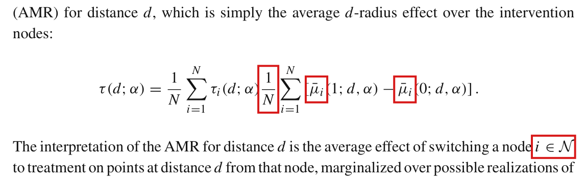
(S4) Circle averages and the AMR [Section 2.2, p. 143 (PDF p. 6)]. “$\mu_i(\mathbf{Y}(\mathbf{z}); d) = \frac{1}{|\{x : d_i(x) = d\}|}\int_{x : d_i(x) = d} Y_x(\mathbf{z})\,\mathrm{d}\zeta$, where $d_i(x) = ||x(i) - x||$ is some well-defined metric that defines whether point $x$ is within a specified distance from intervention node $i$, which is located at $x(i)$, and $\zeta$ is a suitable integration measure.” “$\mu_i(z; d, \alpha) = \mathrm{E}_{\mathbf{Z}_{-i}}[\mu_i(\mathbf{Y}(z, \mathbf{Z}_{-i}); d)]$ is the potential $d$-radius circle average around node $i$, given that node $i$ is assigned to treatment condition $z$ and marginalizing over possible assignments to other points.” “$\tau_i(d; \alpha) = \mu_i(1; d, \alpha) - \mu_i(0; d, \alpha)$, is the average of individualistic responses for points along the circle of radius $d$ around node $i$.” The AMR for distance $d$ is denoted $\tau(d;\alpha)$; its display is misprinted (P008-T14 gives it as printed and corrected): $\tau(d;\alpha) = \frac{1}{N}\sum_{i=1}^{N}\tau_i(d;\alpha)$.
(S5) Estimator [Section 2.3, pp. 143–144 (PDF pp. 6–7)]. “the preferred estimator for practical purposes is the Hajek estimator (Särndal et al. 1992, pp. 182-184), given by: $\widehat{\tau}_{HA}(d) = \frac{1}{N_1}\sum_{i=1}^{N} Z_i\mu_i(\mathbf{Y}; d) - \frac{1}{N_0}\sum_{i=1}^{N}(1 - Z_i)\mu_i(\mathbf{Y}; d)$ where $N_1 = \sum_{i=1}^{N} Z_i$ and $N_0 = N - N_1$.” Here $\mu_i(\mathbf{Y}; d)$ is the circle average of the observed outcomes.
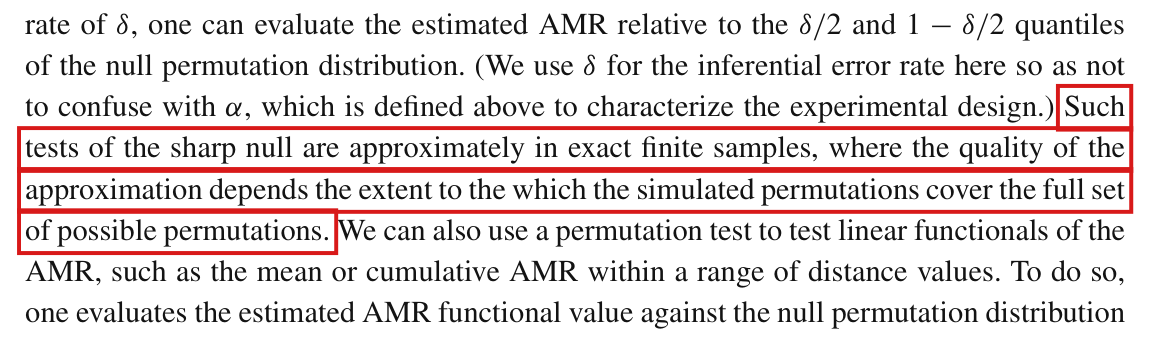
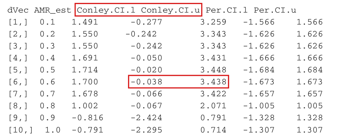
(S6) Hypotheses and the two inference methods [Section 2.3, p. 144 (PDF p. 7)]. “The sharp null hypothesis states that the interventions have no effects whatsoever, such that $Y_x(\mathbf{Z}) = Y_x(\mathbf{0})$ , in which case all unit-level effects are also zero and the AMR is zero. If one assumes that the sharp null hypothesis holds, then the randomization distribution of the AMR can be simulated by simply permuting treatment assignment, estimating the AMR under each of these permutations, and then collecting the resulting set of estimates (Imbens and Rubin 2015, Ch. 5). The resulting distribution is referred to as the null permutation distribution.” The weak null hypothesis is “that the AMR equals zero”. The second method “provides confidence intervals that combine a normal approximation with a nonparametric spatial heteroskedasticity and autocorrelation consistent (spatial-HAC) standard error estimator as proposed by Conley (1999).”
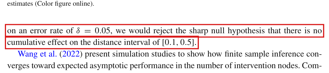
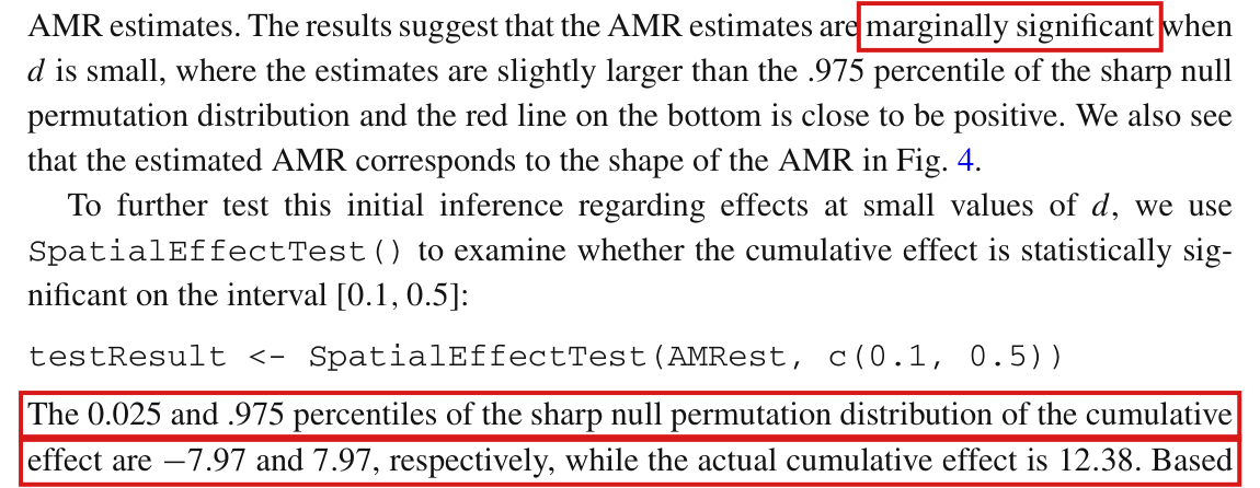
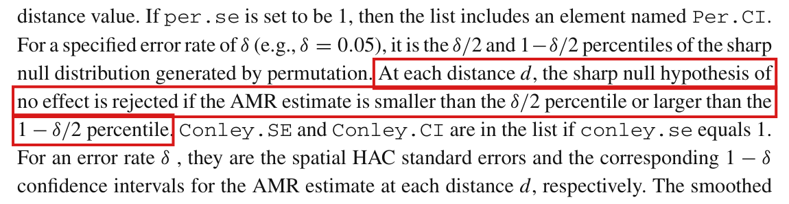
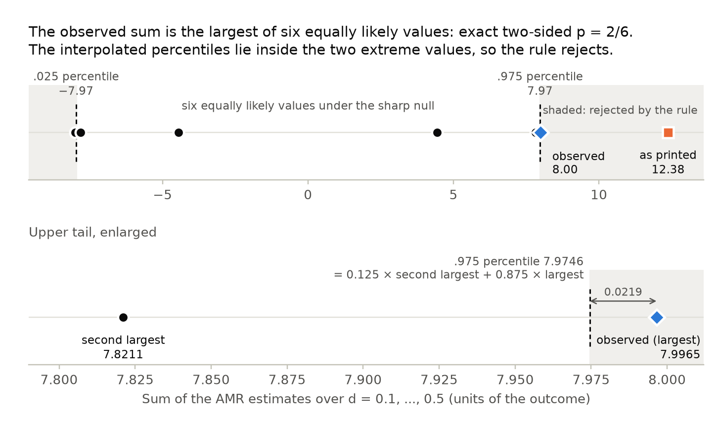
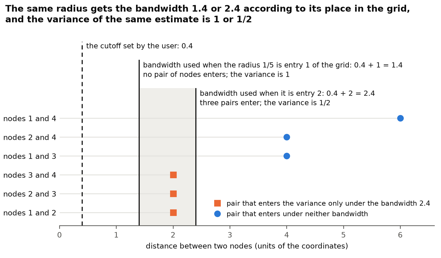
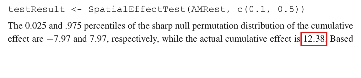
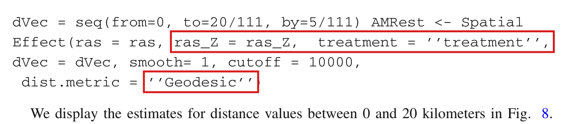
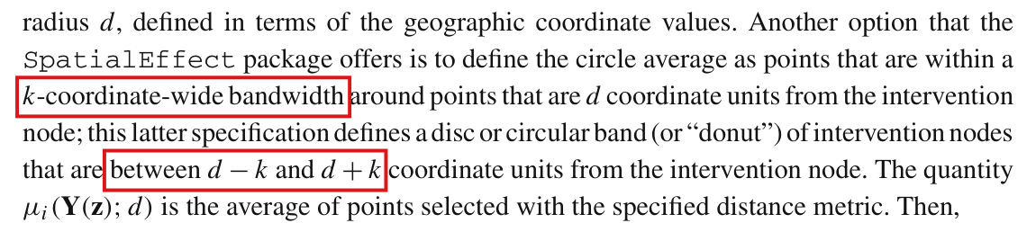
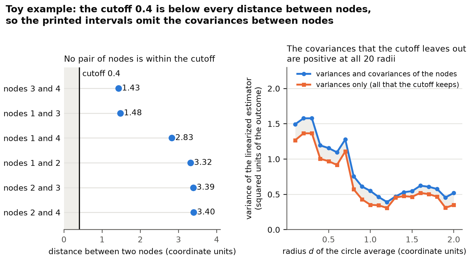
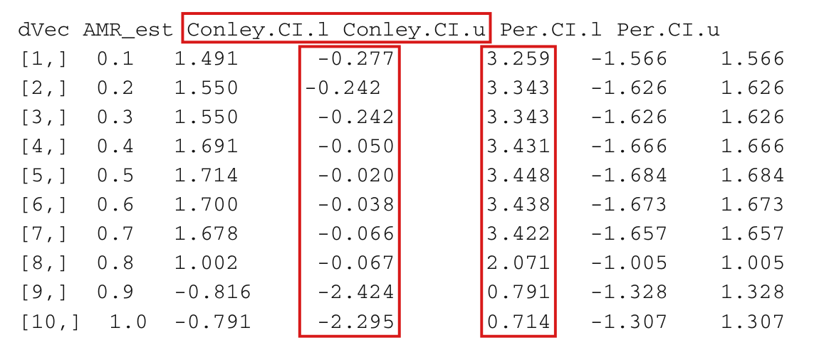
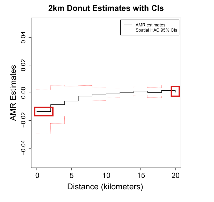
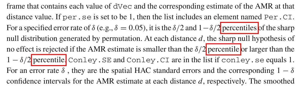
(S7) Package conventions [Section 3, pp. 145–146 (PDF pp. 8–9)]. [p. 145] “Users can choose a set of points that form the edge of a circle of radius $d$, that form a circular band (“donut”) centered at radius $d$, or that form a sector centered at $d$ (“disk”), by altering the option cType. When ras_Z is provided, the distance will be calculated from the boundary of each polygon and we implement polygon intervention. Otherwise, it is calculated from the center of each intervention node and point intervention is implemented.” [p. 145] “For the asymptotic variance estimator, users need to specify a distance threshold (cutoff) beyond which interference dependence does not exist.” [p. 146] “For a specified error rate of $\delta$ (e.g., $\delta = 0.05$), it is the $\delta/2$ and $1-\delta/2$ percentiles of the sharp null distribution generated by permutation. At each distance $d$, the sharp null hypothesis of no effect is rejected if the AMR estimate is smaller than the $\delta/2$ percentile or larger than the $1 - \delta/2$ percentile.” [p. 146] “The SpatialEffectTest() function generates the null permutation distribution of the sum of the AMR estimates within the specified range.”
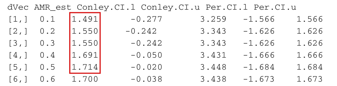
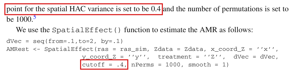
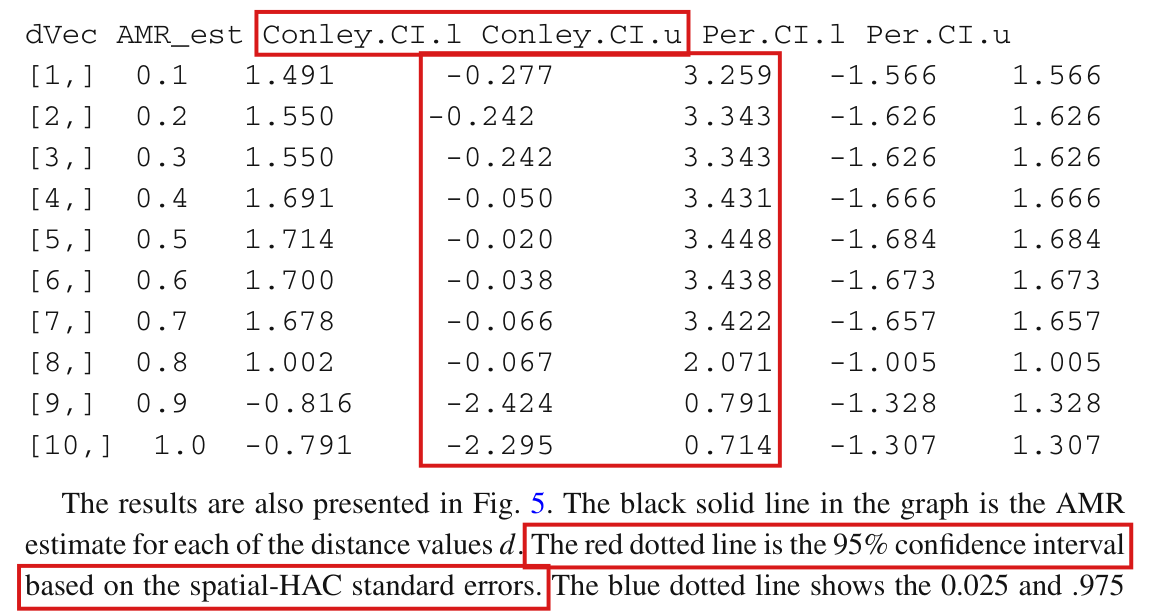
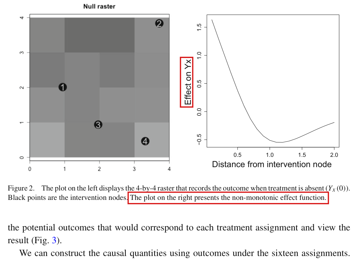
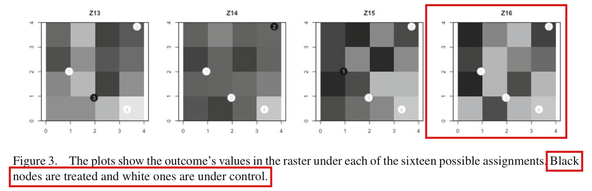
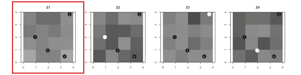
(S8) Toy example [Sections 4–5, pp. 146–150 (PDF pp. 9–13)]. “The toy example includes 4 intervention nodes in a spatial field where outcomes are recorded in a 4-by-4 raster (left plot of Fig. 2).” “We suppose Bernoulli random assignment of the nodes to treatment, in which case there are 16 ways treatment could be applied, all with equal probability.” [pp. 147–148] “we choose dVec to be a sequence from 0.1 to 2 with an interval length of 0.1. The cutoff point for the spatial HAC variance is set to be 0.4 and the number of permutations is set to be 1000.” Footnote 5 [p. 148]: “The number doesn't make any difference here as there are in total 6 assignments.” (The six assignments are those with two of the four nodes treated, as in the observed assignment.)
(S9) Points the paper leaves open, fixed here so that the targets are definite (these are conventions of this file, not statements of the paper). (i) The paper does not say how a “quantile” or “percentile” of a finite permutation distribution is computed. The staged implementations call R's quantile() with its default rule (type 7): for order statistics $x_{(1)} \le \dots \le x_{(n)}$ and $q \in [0,1]$, with $h = 1 + (n-1)q$, $j = \lfloor h \rfloor$ and $g = h - j$, $Q_7(q) = (1-g)x_{(j)} + g\,x_{(j+1)}$ (and $Q_7(1) = x_{(n)}$). The printed toy percentiles $\mp 7.97$ are reproduced by this rule and lie strictly inside the range of the six enumerated values. (ii) $Y_{ix}(z;\alpha)$ uses $Y_x(z, \mathbf{z}_{-i})$ for every $\mathbf{z}_{-i} \in \mathcal{Z}_{-i}$ and both $z \in \{0,1\}$; a statement below that uses it assumes potential outcomes are defined at each such argument (for instance on all of $\{0,1\}^N$). (iii) $\mathcal{Z}$ is finite, so every expectation over $\mathbf{Z}$ is a finite sum. For a finite set of outcome points with counting measure the circle average is the arithmetic mean over the points with $d_i(x) = d$; every example below is of this kind or has outcomes constant on the circles concerned. (iv) The paper has no numbered results, no appendix and no proofs; every target is an unnumbered statement or display, located by page.
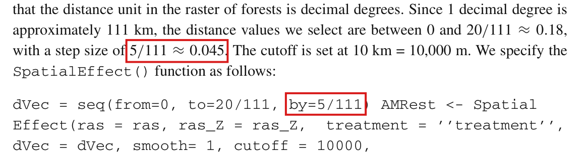
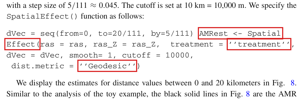
Scope of the list. The paper is a tutorial with no numbered results and no proofs. Three of its eight headline claims contain mathematical statements and enter as headline targets: P008-H1 (the definition of the AMR and its circle-average identities, P008-T25), P008-H2 (the sharp and weak null hypotheses, P008-T26, and the attributed consistency and normality statement, P008-T28) and P008-H6 (the additive case of the attributed equivalence with a structural coefficient, P008-T27). P008-H3, P008-H4 and P008-H5 are a simulated illustration, an empirical estimate and its interpretation; P008-H7 and P008-H8 describe the method and the package. Twelve confirmed errors have corrections that change a mathematical statement, a formula or a constant and are targets: P008-N012 (Major; the reference law of the Uganda permutation test), P008-E002 (Moderate; the percentile rule and the toy example's rejection), P008-N002 (Moderate; the toy example's cutoff), P008-N016 (Moderate; the sum of AMR estimates read as a change in a probability), P008-E015 (Moderate; the bandwidth formula of the archived variance code), P008-E003 (Minor; 12.38 for 8.00), P008-E004 (Minor; the step 5/111 for 0.5/111), P008-E005 (Minor; the misprinted display of the AMR), P008-E007 (Minor; the band described as a set of intervention nodes), P008-N001 (Minor; the band as described and as implemented), P008-N004 (Minor; the scale of the effect function in Figure 2) and P008-N009 (Minor; what the estimate at distance 0 averages). P008-E015, P008-N001, P008-N004 and P008-N009 set a sentence or figure of the article against the staged package or vignette, which is a later snapshot than the release the article cites; they are listed because each rests on an exact formal example or derivation and its correction replaces a formula, a constant or the description of the set that is averaged, and each target says which premise is read from source code and lies outside what Lean can establish. The other nine confirmed errors are not targets because their corrections change no mathematical statement: P008-N017 (Moderate) is the horizontal placement of the band estimates in the bottom panel of Figure 8, established by recalculation from archived data (the band convention on which it rests is P008-T17 (b)); P008-E006 is an argument name; P008-E009 and P008-E012 concern the typesetting of the printed calls, an input guard of the later package and the wording of a numerical default; P008-N006 and P008-N007 concern the reproducibility of the toy intervals and of the smoothed curve with the staged copies of the package; P008-N005 is the colour key of Figure 3; P008-E010 is copy-editing (the mathematical content of the garbled sentence of p. 144 is in P008-T3, P008-T4 and P008-T22); P008-E011 is bibliographic. Findings classed as a clarity note (P008-E008), as not confirmed (P008-E001, P008-N003, P008-N013), as undetermined (P008-N008, P008-N010, P008-N011, P008-N014, P008-N015) or as out of scope (P008-E013, P008-E014) are outside the brief.
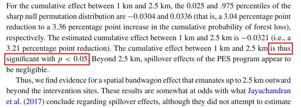
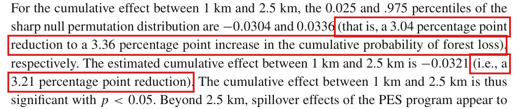
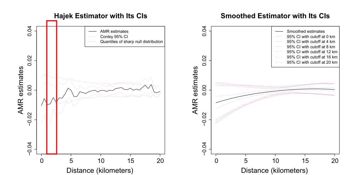
Effective claim (source TeX): [Printed statement] “For the cumulative effect between 1 km and 2.5 km, the 0.025 and .975 percentiles of the sharp null permutation distribution are $-0.0304$ and $0.0336$ (that is, a 3.04 percentage point reduction to a 3.36 percentage point increase in the cumulative probability of forest loss), respectively. The estimated cumulative effect between 1 km and 2.5 km is $-0.0321$ (i.e., a 3.21 percentage point reduction). The cumulative effect between 1 km and 2.5 km is thus significant with $p < 0.05$. Beyond 2.5 km, spillover effects of the PES program appear to be negligible.”
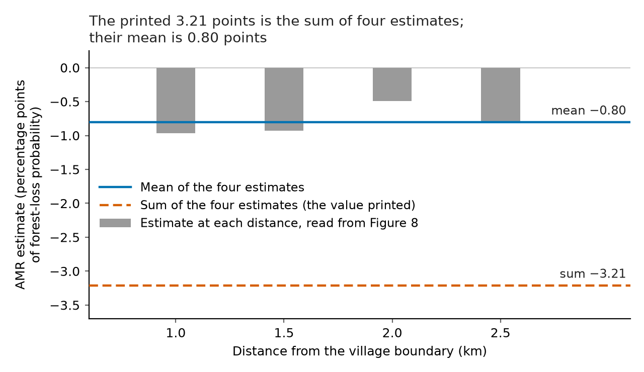
[Claim refuted] That the unweighted sum of the AMR estimates (or of the AMRs) over the distances evaluated in a range is, after multiplication by 100, a change in percentage points of a probability of forest loss.
Counterexample (the validator's adjudicated construction; integer and rational arithmetic; a synthetic population, not Uganda data). Distances in kilometres.
1. $N = 4$ nodes with centres $c_0 = (0,0)$, $c_1 = (20,0)$, $c_2 = (0,20)$, $c_3 = (20,20)$. Radii $d_1, \dots, d_4 = 1, 3/2, 2, 5/2$. Let $M = 40000$ and, for $k = 1, \dots, M$, $\ell_k = 2k - M - 1$, $u_k = (M^2 - \ell_k^2)/(M^2 + \ell_k^2)$, $v_k = 2M\ell_k/(M^2 + \ell_k^2)$ and $x_{i,j,k} = c_i + d_j(u_k, v_k)$. The field is $\mathcal{X} = \{c_0, c_1, c_2, c_3\} \cup \{x_{i,j,k} : i = 0,\dots,3;\ j = 1,\dots,4;\ k = 1,\dots,M\}$, with Euclidean distance and counting measure.
2. $u_k^2 + v_k^2 = 1$, so $\|x_{i,j,k} - c_i\| = d_j$; the directions $(u_k, v_k)$ are distinct ($v_k/(1 + u_k) = \ell_k/M$ is strictly increasing in $k$); every point within $5/2$ of $c_i$ is at least $35/2$ from the other centres. Hence $|\mathcal{X}| = 640004$ and, for each $i$ and $j$, $\{x \in \mathcal{X} : \|x - c_i\| = d_j\} = \{x_{i,j,k} : k = 1,\dots,M\}$ has exactly $M$ points.
3. Design: $Z_0, \dots, Z_3$ independent Bernoulli(1/2). With $B = (B_0, B_1, B_2, B_3) = (400, 1000, 400, 1000)$, for every $\mathbf{z} \in \{0,1\}^4$: $Y_{c_i}(\mathbf{z}) = 0$ and $Y_{x_{i,j,k}}(\mathbf{z}) = \mathbf{1}\{k \le B_i - 321 z_i\}$. All potential outcomes are in $\{0, 1\}$ (1 = loss).
4. For every $i$, $j$ and $b \in \{0,1\}$: $\mu_i(b; d_j, \alpha) = (B_i - 321 b)/40000$, so $\tau_i(d_j; \alpha) = -321/40000$ and $\tau(d_j; \alpha) = -321/40000 = -0.008025$.
5. At the assignment $\mathbf{z}^* = (1,1,0,0)$ (probability $1/16$): $\widehat{\tau}_{HA}(d_j) = \frac{79 + 679}{2 \cdot 40000} - \frac{400 + 1000}{2 \cdot 40000} = -\frac{321}{40000}$ for each $j$, and the unweighted sum over the four radii is $\sum_{j=1}^{4}\widehat{\tau}_{HA}(d_j) = \sum_{j=1}^{4}\tau(d_j;\alpha) = -321/10000 = -0.0321$.
6. The probability of loss at a point drawn uniformly from the $640000$ circle points (equivalently: a uniformly drawn node, radius and circle point) is $Q_0 = (400 + 1000 + 400 + 1000)/160000 = 7/400$ when the point's own node is untreated and $Q_1 = (79 + 679 + 79 + 679)/160000 = 379/40000$ when it is treated; $Q_1 - Q_0 = -321/40000 = -0.008025$, i.e. $-0.8025$ percentage points, not $-3.21$. Every other normalized weighting of the four radii gives the same difference, because $\tau(d_j;\alpha)$ does not depend on $j$. Read as a change in this probability, the sum would give $Q_0 + (-321/10000) = -73/5000 < 0$.
7. Companion model on the same field: $Y_{c_i}(\mathbf{z}) = 0$ and $Y_{x_{i,j,k}}(\mathbf{z}) = 1 - z_i$. Then $\tau(d_j;\alpha) = -1$ for each $j$, the sum over the four radii is $-4$, and the sum of the Hajek estimates at $\mathbf{z}^*$ is $-4$. Since $a - b \ge -1$ for all $a, b \in [0,1]$, $-4$ is not the difference of two probabilities of any event.
: SAP.P008a.T7WholeStatement
Theorem: SAP.P008a.T7
Statement hash: 18f3b8ba7240c179b53bfbdc37e0dfbe8334e5a52c989bcd3454e192d15d584e
Statement definition: SAP.P008a.T7WholeStatement
Certificate. 20261104T160817Z
Declaration review: faithful; 2026-11-04T16:30:26Z; binding v2
Evidence scope: Certification checks formal proof objects. Statement fidelity is a model judgment. Author review is separate.
Proof dependencies: Independently extracted
Manifest annotation reconciliation: Effective use follows the source-bound dependency observation; original annotations are retained in the crosswalk.
AronowAudit.P008.binary_companion_counterexample: observed used
AronowAudit.P008.binary_count_mean: observed used
AronowAudit.P008.risk_sampling_probabilities: observed used
AronowAudit.P008.summed_risk_counterexample: observed used
Source and evidence metadata · sap-2026-11-08-assured-release















My comment and the history of this entry