Assumptions and verification
Claim revision: catalog:14e734c0b6afdfa4e2a82b4d6daa9ad75814faeb14f65b39d3a9464d77aaeb1a
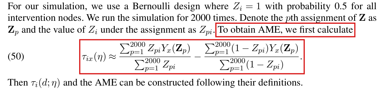
Standing assumptions: Source: Wang, Samii, Chang and Aronow, 'Design-Based Inference for Spatial Experiments under Unknown Interference', Annals of Applied Statistics (2025), printed pp. 744-768 (main.pdf, 25 pp.), and its Supplement A (supplements/supplement-a.pdf, 40 pp., which holds every proof). 'p. 754 (PDF p. 11)' is a page of the article; 'Supplement A p. 15' is the supplement's own page number (its PDF page has the same number). Quotations are verbatim from the page images; a bracketed remark inside a quotation is not the paper's text.
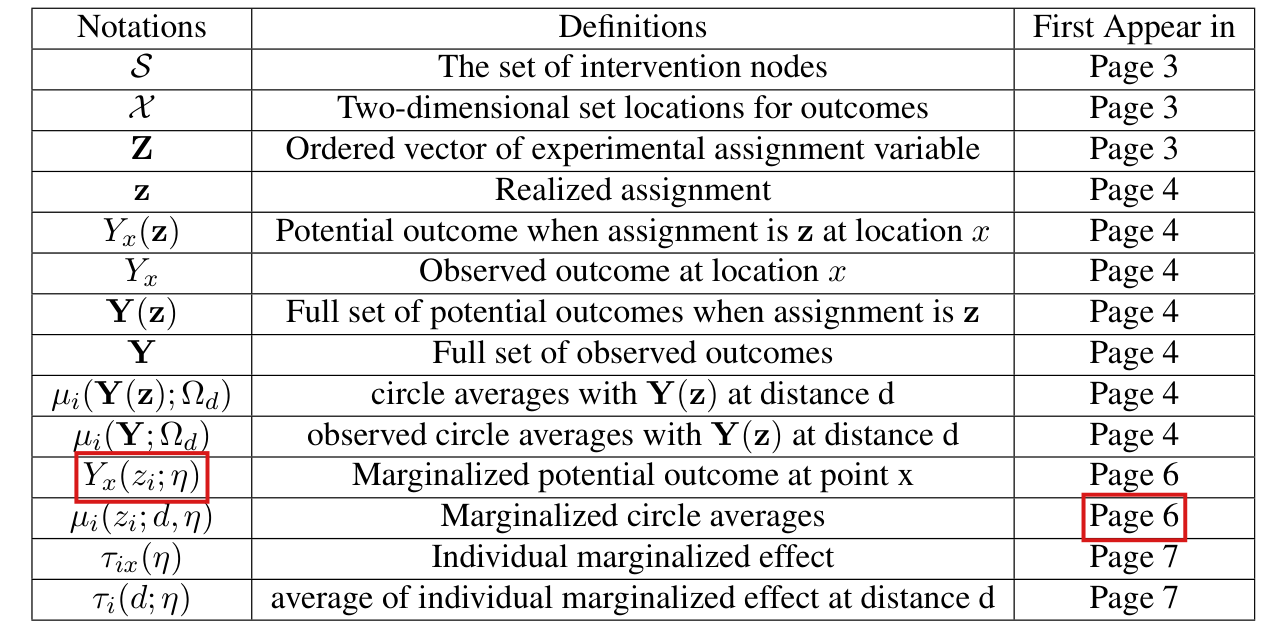
(S1) Setting [Section 2, pp. 746-747 (PDF pp. 3-4)]. 'Suppose a set of intervention nodes $\mathcal S=\{1,\ldots,N\}$. Each node $i\in\mathcal S$ can be either a point or a collection of points (e.g., a polygon) that resides in a two-dimensional set $\mathcal X$ indexed by $x=(x_1,x_2)$ (e.g., latitude and longitude). An experimental design assigns a binary treatment $Z_i\in\{0,1\}$ to each intervention node. The ordered vector of experimental assignment variables is $\mathbf Z\equiv(Z_1,\ldots,Z_N)$, and the ex post realized assignment from the experiment is given by $\mathbf z\equiv(z_1,\ldots,z_N)\in\{0,1\}^N$. The experimental design fixes the set of possible assignment vectors as well as a probability distribution over that set. Our analysis considers the case of Bernoulli randomization for each $Z_i$, that is, (possibly weighted) coin flips to determine treatment status at each node.' 'Potential outcomes at any point $x\in\mathcal X$ are defined for each value of $\mathbf z$, $(Y_x(\mathbf z))_{\mathbf z\in\{0,1\}^N}$. Given a realized treatment assignment $\mathbf z$, we observe the corresponding potential outcome at $x$, (1) $Y_x=\sum_{\mathbf z\in\{0,1\}^N}Y_x(\mathbf z)I(\mathbf Z=\mathbf z)$, where $I(\cdot)$ is the indicator function and $I(\mathbf Z=\mathbf z)$ takes on the value 1 if the random assignments $\mathbf Z$ realize to be $\mathbf z$ and 0 otherwise.' 'Let $\mathbf Y(\mathbf z)=(Y_x(\mathbf z))_{x\in\mathcal X}$ denote the full set of potential outcomes when $\mathbf Z=\mathbf z$ and $\mathbf Y=(Y_x)_{x\in\mathcal X}$ denote the full set of realized outcomes.' (pp. 747-748) 'For our design-based inference, the only source of stochastic variation is from $\mathbf Z$.' Potential outcomes and (in Section 6.4) confounders are fixed; every expectation, variance and probability is over $\mathbf Z$.
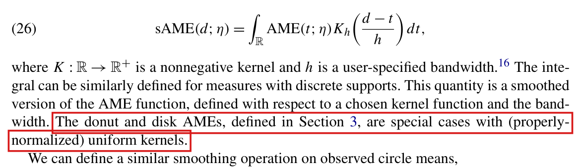
(S2) Circle averages [Section 2, p. 747 (PDF p. 4)]. 'For $i\in\mathcal S$, we define (2) $\mu_i(\mathbf Y(\mathbf z);\Omega_d)=\frac{\int_{x:d_i(x)\in\Omega_d}Y_x(\mathbf z)\,\mathrm d\zeta}{\int_{x:d_i(x)\in\Omega_d}\mathrm d\zeta}$. In the expression above, $d_i(x)$ measures the distance between point $x$ and intervention node $i$. When $i$ is a point located at $x(i)$, $d_i(x)=\gamma(x(i),x)$, where $\gamma(\cdot,\cdot)$ is a well-defined metric (e.g., Euclidean, geodesic, or a least-cost distance) that satisfies the triangular inequality. If $i$ is a collection of points, then $d_i(x)=\min_{x'\in i}\|x'-x\|$, the minimal distance between $x$ and points belonging to $i$. $\Omega_d$ is a set of distance values, and $\zeta$ is a suitable measure on $\mathcal X$. Therefore, $\mu_i(\mathbf Y(\mathbf z);\Omega_d)$ is the average outcome across points whose distance to $i$ falls in $\Omega_d$.' 'If the points in $\mathcal X$ are dense and spaced evenly, then $\Omega_d$ could be a singleton, $\Omega_d=\{d\}$. ... $\Omega_d$ could be a donut, where $\Omega_d=[d-\kappa,d]$ (with $\kappa$ a user-chosen constant dictating the donut's thickness), or a disk, where $\Omega_d=[0,d]$. ... When it does not cause confusion, we write $\mu_i(\mathbf Y(\mathbf z);\Omega_d)$ simply as $\mu_i(\mathbf Y(\mathbf z);d)$. Similarly, the realized circle average for intervention node $i$ at $d$ is (3) $\mu_i(\mathbf Y;d)=\sum_{\mathbf z\in\{0,1\}^N}\mu_i(\mathbf Y(\mathbf z);d)I(\mathbf Z=\mathbf z)$.' The article notes (p. 747) that data 'may come in various formats including raster data or data on a discrete set of points in $\mathcal X$'.
(S3) Marginalized quantities and the AME [Section 3, pp. 748-750 (PDF pp. 5-7)]. 'To define the spatial AME, first rewrite the potential outcome at point $x$ as $Y_x(z_i,\mathbf z_{-i})$, where $\mathbf z_{-i}$ is a vector equaling $\mathbf z$, except that the value for intervention node $i$ is omitted.' '(4) $Y_{ix}(z_i;\eta)=\mathrm E_{\mathbf Z_{-i}}[Y_x(z_i,\mathbf Z_{-i})]=\sum_{\mathbf z_{-i}\in\{0,1\}^{N-1}}Y_x(z_i,\mathbf z_{-i})\Pr(\mathbf Z_{-i}=\mathbf z_{-i};\eta)$, where $\eta$ is an experimental design parameter indexing the distribution of $\mathbf Z$ (i.e., the probability of treatment assignments).' '(5) $\mu_i(z_i;d,\eta)=\mathrm E_{\mathbf Z_{-i}}[\mu_i(\mathbf Y(z_i,\mathbf Z_{-i});d)]=\sum_{\mathbf z_{-i}\in\{0,1\}^{N-1}}\mu_i(\mathbf Y(z_i,\mathbf z_{-i});d)\Pr(\mathbf Z_{-i}=\mathbf z_{-i};\eta)$, where we use $\mathbf Y(z_i,\mathbf z_{-i})$ to denote the vector of potential outcomes over points in $\mathcal X$ that obtain under treatment assignment $(z_i,\mathbf z_{-i})$.' 'Due to linearity of expectation, we also have (6) $\mu_i(z_i;d,\eta)=\frac{\int_{x:d_i(x)\in\Omega_d}Y_{ix}(z_i;\eta)\,\mathrm d\zeta}{\int_{x:d_i(x)\in\Omega_d}\mathrm d\zeta}$.' '(7) $\tau_{ix}(\eta)=Y_{ix}(1;\eta)-Y_{ix}(0;\eta)$.' '(8) $\tau_i(d;\eta)=\mu_i(1;d,\eta)-\mu_i(0;d,\eta)$.' 'Finally, define the average marginalized effect (AME) for distance $d$ by taking the mean over the intervention nodes, (9) $\mathrm{AME}(d;\eta)=\frac1N\sum_{i=1}^N\tau_i(d;\eta)$.' (p. 750) 'our analysis focuses on experimental designs with Bernoulli assignment, in which case the possible assignments consist of the $2^N$ possible vectors that could be obtained from $N$ (possibly differentially weighted) coin flips.'
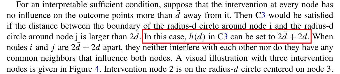
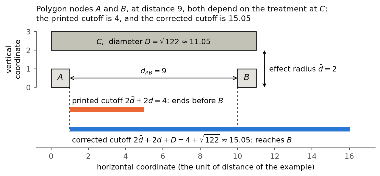
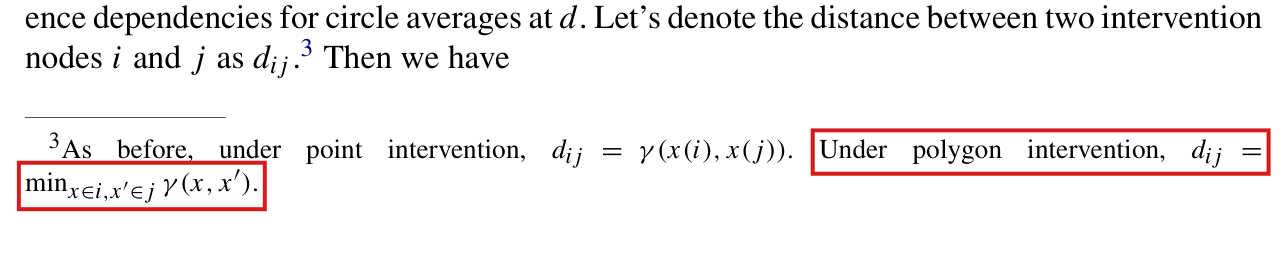
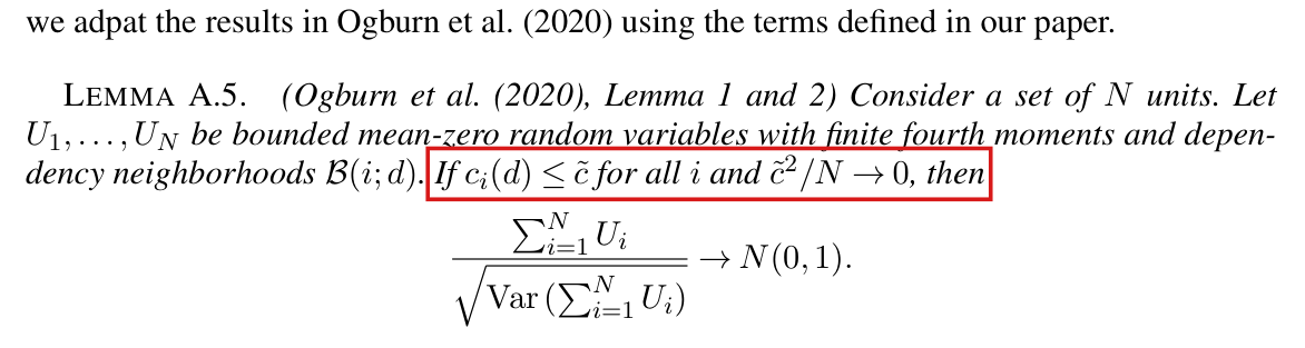
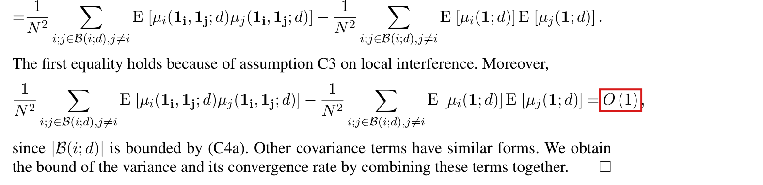
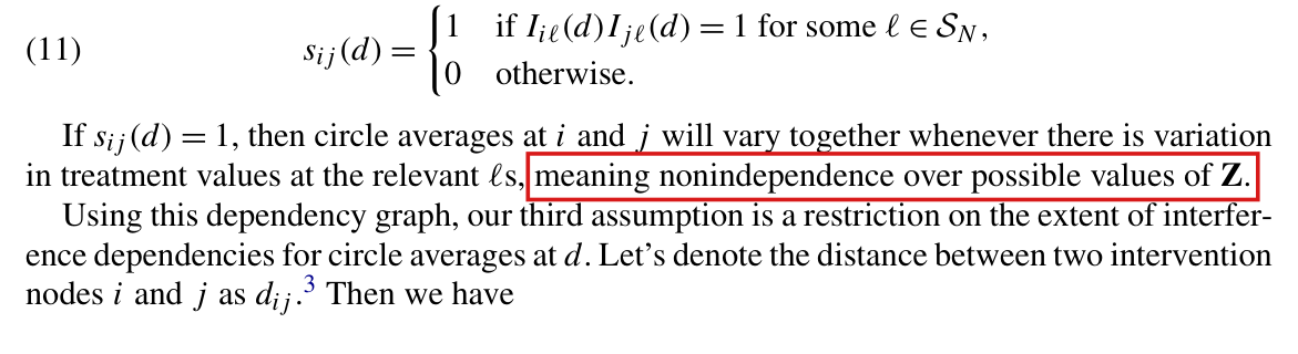
(S4) Inferential assumptions [Section 4, pp. 751-753 (PDF pp. 8-10)]. 'Our asymptotic analysis considers a sequence of sets indexed by the sample size $N$. The set of intervention nodes is denoted as $\mathcal S_N$ and the set of outcome points $\mathcal X_N$. Note that assumptions below are assumed to hold uniformly for all large sample sizes.' 'C1 (Bernoulli design). $(Z_1,\ldots,Z_N)$ is a vector of independent Bernoulli($p$) draws.' 'C2 (Bounded potential outcomes). $|Y_x(\mathbf z)|<b$ for some finite constant $b$ and all $x\in\mathcal X$ and $\mathbf z\in\{0,1\}^N$.' 'We work with the assumption that the assignment probability, $p$, is constant over intervention nodes and discuss the extension to cases where assignment probabilities vary in Section 6.4 below.' 'Let $I_{ij}(d)$ be an indicator for whether assignment at intervention node $j$ interferes with the $d$-radius circle average at node $i$, (10) $I_{ij}(d)=1$ if $\mu_i(\mathbf Y(\mathbf z);d)\neq\mu_i(\mathbf Y(\mathbf z');d)$ for some $\mathbf z,\mathbf z'\in\{0,1\}^N$ such that $\mathbf z_{-j}=\mathbf z'_{-j}$; $I_{ij}(d)=1$ if $i=j$; $I_{ij}(d)=0$ otherwise. Then, let $s_{ij}(d)$ be an indicator for whether $d$-radius circle averages at $i$ and $j$ are subject to interference from treatment at some common intervention node $\ell$ (which could be $i$, $j$, or some other third intervention node), (11) $s_{ij}(d)=1$ if $I_{i\ell}(d)I_{j\ell}(d)=1$ for some $\ell\in\mathcal S_N$; $s_{ij}(d)=0$ otherwise.' 'Let's denote the distance between two intervention nodes $i$ and $j$ as $d_{ij}$.' Footnote 3: 'As before, under point intervention, $d_{ij}=\gamma(x(i),x(j))$. Under polygon intervention, $d_{ij}=\min_{x\in i,x'\in j}\gamma(x,x')$.' 'C3 (Local interference.). Let $h:[0,\infty)\to[0,\infty)$ be a function independent of sample sizes. For each $d$ and all large sample sizes $N$ and all pairs of intervention nodes $i$ and $j$ in $\mathcal S_N$, there exists a constant $h(d)$ such that if $d_{ij}>h(d)$, then $s_{ij}(d)=0$.' 'This assumption hence implies that, for $i$, $j$ with $d_{ij}>h(d)$, $\mu_i(Y(z,\mathbf Z_{-i});d)$ and $\mu_j(Y(z',\mathbf Z_{-j});d)$ are independent of each other over $\mathbf Z$.' 'Define $\mathcal S_N(i;d)\equiv\{j\in\mathcal S_N:d_{ij}\le d\}$, the set of intervention nodes whose distance to node $i$ is less than $d$.' 'C4 (Intervention node spacing). Let $b:[0,\infty)\to[0,\infty)$ be a function independent of sample sizes. For each $d$ and all large sample sizes $N$, the sequence of intervention nodes satisfies $\sup_{i\in\mathcal S_N}|\mathcal S_N(i;d)|\le b(d)$.' 'Let's define the neighborhood $\mathcal B(i;d)$ that includes all the nodes whose circle averages at $d$ may interfere with that of node $i$, (12) $\mathcal B_N(i;d)=\{j\in\mathcal S_N:d_{ij}\le h(d)\}$. From C3 we know that $s_{ij}(d)=0$ for $j\notin\mathcal B_N(i;d)$. From C4 we know that $|\mathcal B_N(i;d)|\le b(h(d))$. Define $c_i(d)=|\mathcal B_N(i;d)|$ and $c_N(d)=\max_{i\in\mathcal S_N}c_i(d)$. Conditions C3 and C4 imply the following condition: C4A (Limited local interference with respect to $d$). For each $d$, $c_N(d)=O(1)$.' 'In our analyses below, we suppress the subscripts for asymptotic sequences unless they are needed to add clarity.' Since $d_{ii}=0\le h(d)$, $i\in\mathcal B_N(i;d)$.
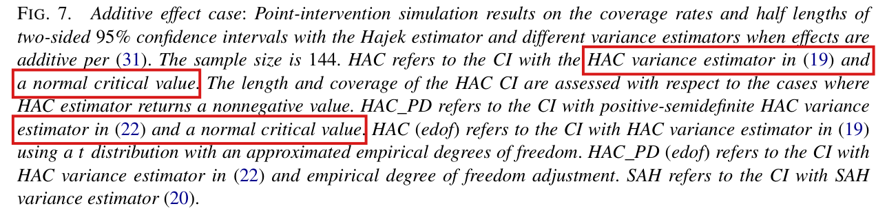
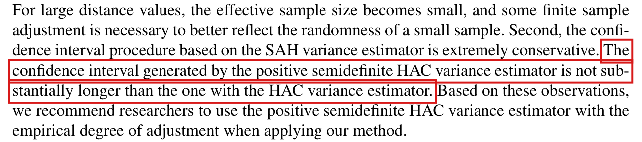
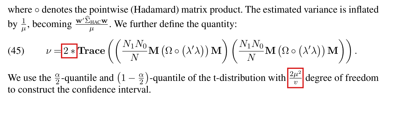
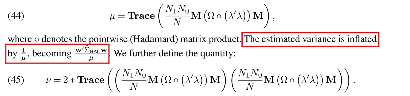
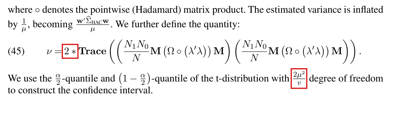
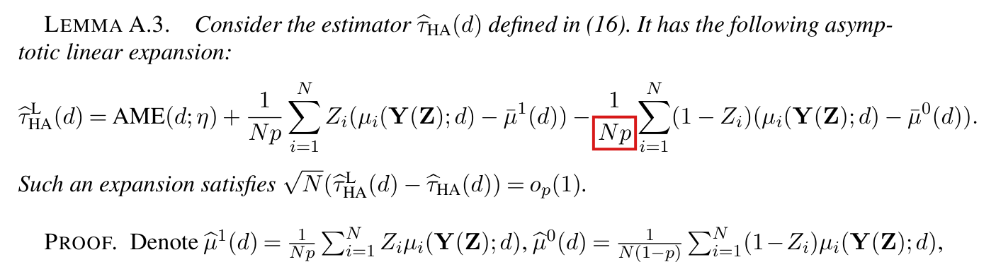
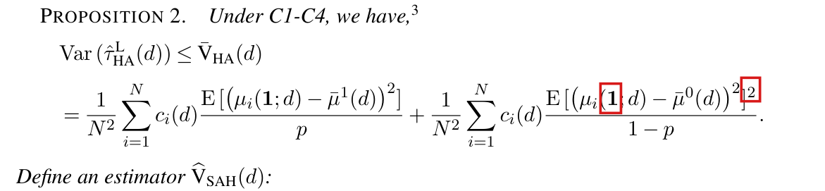
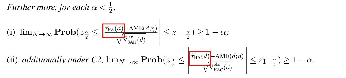
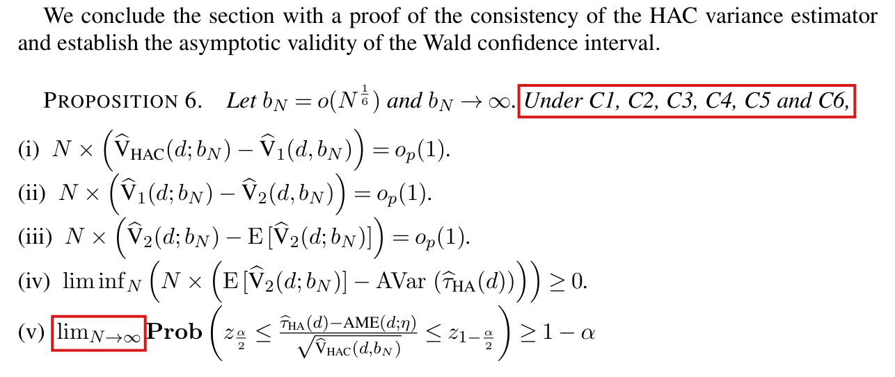
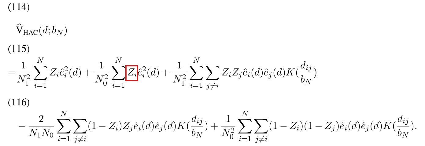
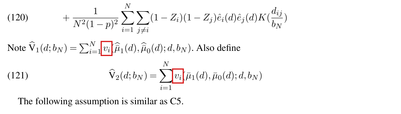
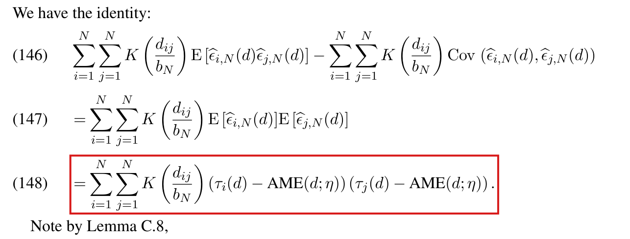
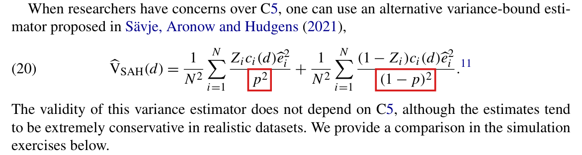
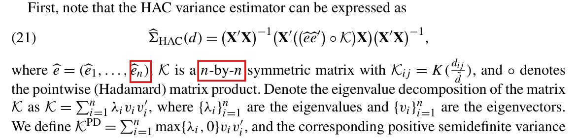
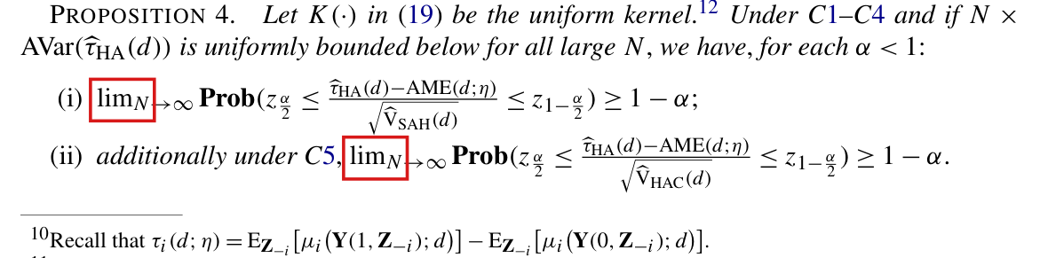
(S5) Estimators and variance estimators [Section 5, pp. 754-756 (PDF pp. 11-13)]. '(13) $\hat\tau_{\mathrm{HT}}(d)=\frac1{Np}\sum_{i=1}^NZ_i\mu_i(\mathbf Y;d)-\frac1{N(1-p)}\sum_{i=1}^N(1-Z_i)\mu_i(\mathbf Y;d)$.' 'the Hajek estimator replaces them with $N_1=\sum_{i=1}^nZ_i$ and $N_0=N-N_1$, respectively, (16) $\hat\tau_{\mathrm{HA}}(d)=\frac1{N_1}\sum_{i=1}^NZ_i\mu_i(\mathbf Y;d)-\frac1{N_0}\sum_{i=1}^N(1-Z_i)\mu_i(\mathbf Y;d)$.' [The upper limit $n$ in $N_1$ is a misprint for $N$: finding P004-N001.] '(18) $\binom{\hat\mu_0(d)}{\hat\tau_{\mathrm{HA}}(d)}=\arg\min_{(\mu_0,\tau)}\sum_{i=1}^N(\mu_i(\mathbf Y;d)-\mu_0-\tau Z_i)^2$.' '(19) $\hat\Sigma_{\mathrm{HAC}}(d)=(\mathbf X'\mathbf X)^{-1}\Big(\sum_{i=1}^N\sum_{j=1}^N\mathbf X_i'\mathbf X_j\hat e_i\hat e_jK\big(\frac{d_{ij}}{\tilde d}\big)\Big)(\mathbf X'\mathbf X)^{-1}$, where $\mathbf X=\big(\begin{smallmatrix}1&1&\cdots&1\\Z_1&Z_2&\cdots&Z_N\end{smallmatrix}\big)'\in\mathbb R^{N\times2}$ and $\mathbf X_i$ denotes the $i$th row of the matrix. The $\hat e_i$'s are the residuals from the regression: $\hat e_i=\mu_i(\mathbf Y;d)-\hat\mu_0(d)-\hat\tau_{\mathrm{HA}}(d)Z_i$. $K(\cdot)$ is a kernel function. $\tilde d$ is a cutoff value, and our setup suggests setting it at $\tilde d=h(d)$. The (2,2)-entry of the estimator $\hat\Sigma_{\mathrm{HAC}}(d)$ is our estimator for the variance of $\hat\tau_{\mathrm{HA}}(d)$, and we denote it as $\hat{\mathrm V}_{\mathrm{HAC}}(d)$.' 'C5 (Homophily in treatment effects). For each value $d\ge0$, $\frac1N\sum_{i=1}^N\Big(\big(\tau_i(d;\eta)-\mathrm{AME}(d;\eta)\big)\sum_{j\in\{i\}\cup\mathcal B(i;d)}\big(\tau_j(d;\eta)-\mathrm{AME}(d;\eta)\big)\Big)\ge0$.' Footnote 10: 'Recall that $\tau_i(d;\eta)=\mathrm E_{\mathbf Z_{-i}}[\mu_i(\mathbf Y(1,\mathbf Z_{-i});d)]-\mathrm E_{\mathbf Z_{-i}}[\mu_i(\mathbf Y(0,\mathbf Z_{-i});d)]$.' '(20) $\hat{\mathrm V}_{\mathrm{SAH}}(d)=\frac1{N^2}\sum_{i=1}^N\frac{Z_ic_i(d)\hat e_i^2}{p^2}+\frac1{N^2}\sum_{i=1}^N\frac{(1-Z_i)c_i(d)\hat e_i^2}{(1-p)^2}$.' Footnote 11: 'Recall that $c_i(d)=|\mathcal B_N(i;d)|$.' Footnote 12: '$K(x)=I(x\in[0,1])$.' 'For some $\alpha<1$, let $z_{\frac\alpha2}$ and $z_{1-\frac\alpha2}$ be the $\frac\alpha2$th and $(1-\frac\alpha2)$th quantiles of the standard normal distribution, respectively.' (p. 756) '(21) $\hat\Sigma_{\mathrm{HAC}}(d)=(\mathbf X'\mathbf X)^{-1}\big(\mathbf X'((\hat e\hat e')\circ\mathcal K)\mathbf X\big)(\mathbf X'\mathbf X)^{-1}$, where $\hat e=(\hat e_1,\ldots,\hat e_n)$, $\mathcal K$ is a $n$-by-$n$ symmetric matrix with $\mathcal K_{ij}=K(\frac{d_{ij}}{\tilde d})$, and $\circ$ denotes the pointwise (Hadamard) matrix product. Denote the eigenvalue decomposition of the matrix $\mathcal K$ as $\mathcal K=\sum_{i=1}^n\lambda_iv_iv_i'$, where $\{\lambda_i\}_{i=1}^n$ are the eigenvalues and $\{v_i\}_{i=1}^n$ are the eigenvectors. We define $\mathcal K^{\mathrm{PD}}=\sum_{i=1}^n\max\{\lambda_i,0\}v_iv_i'$, and the corresponding positive semidefinite variance estimator (22) $\hat\Sigma^{\mathrm{PD}}_{\mathrm{HAC}}(d)=(\mathbf X'\mathbf X)^{-1}\big(\mathbf X'((\hat e\hat e')\circ\mathcal K^{\mathrm{PD}})\mathbf X\big)(\mathbf X'\mathbf X)^{-1}$.' [Here too $n$ is a misprint for $N$: P004-N001.]
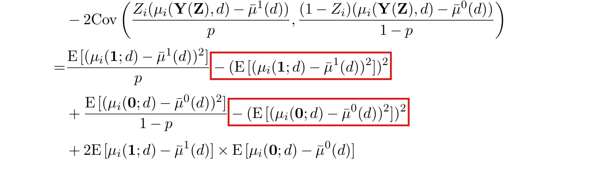
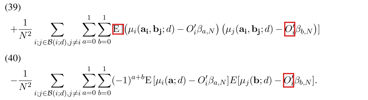
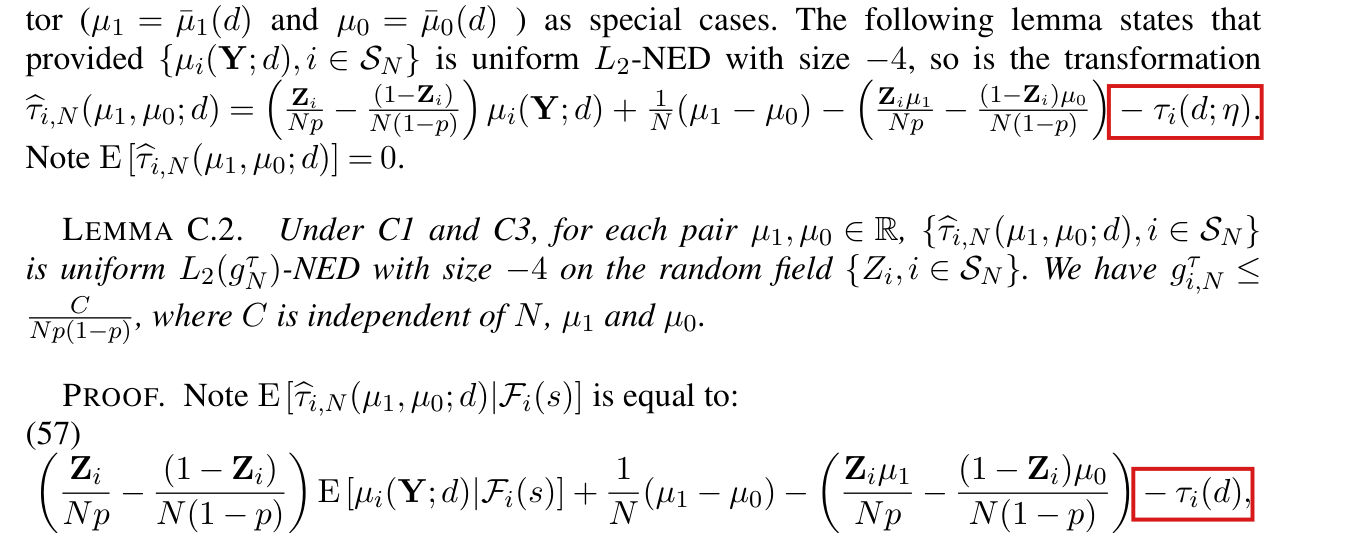
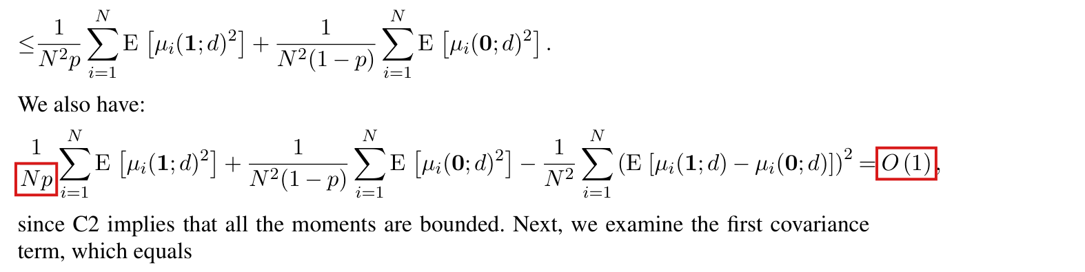
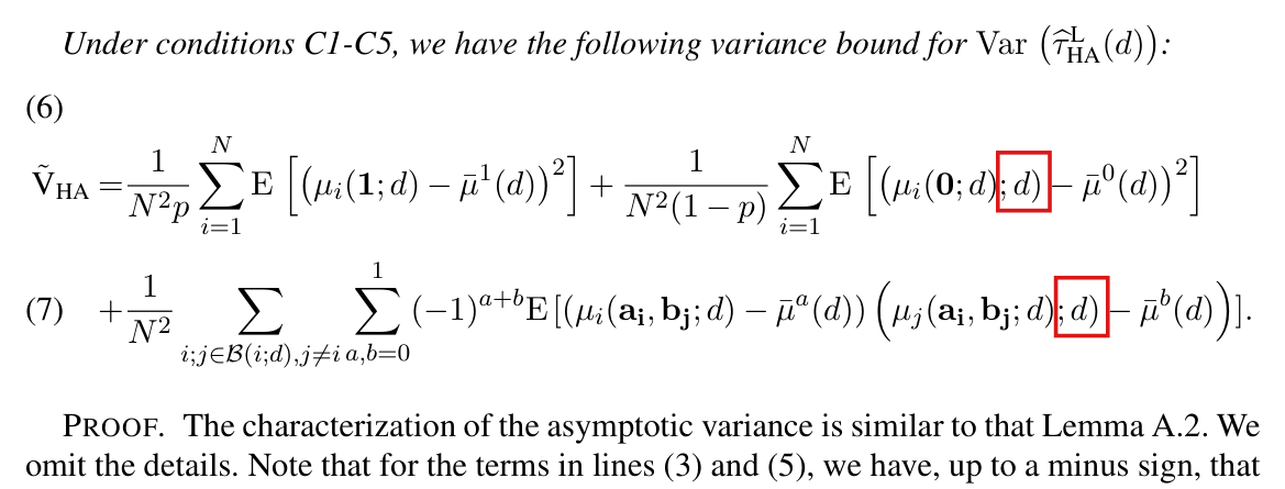
(S6) Conventions of Supplement A [Supplement A p. 1]. 'Without noted otherwise, the expectation is always taken over random assignments $\mathbf Z$.' 'We write $\mathrm E[\mu_i(\mathbf Y(\mathbf Z);d)|Z_i=1]=\mathrm E[\mu_i(\mathbf 1;d)]$ and $\mathrm E[\mu_i(\mathbf Y(\mathbf Z);d)|Z_i=0]=\mathrm E[\mu_i(\mathbf 0;d)]$.' 'We write $\mathrm E[\mu_i(\mathbf Y(\mathbf Z);d)|Z_i=a,Z_j=b]=\mathrm E[\mu_i(\mathbf a_{\mathbf i},\mathbf b_{\mathbf j};d)]$ for $a,b\in\{0,1\}$.' 'We write $\sum_{i=1}^N\sum_{j\in\mathcal B(i;d)}$ as $\sum_{i;j\in\mathcal B(i;d)}$.' So, under independent assignment, $\mathrm E[\mu_i(\mathbf a;d)]=\mu_i(a;d,\eta)$ of (5), and an expression such as $\mathrm E[(\mu_i(\mathbf a_{\mathbf i},\mathbf b_{\mathbf j};d)-c)(\mu_j(\mathbf a_{\mathbf i},\mathbf b_{\mathbf j};d)-c')]$ is the conditional expectation of $(\mu_i(\mathbf Y(\mathbf Z);d)-c)(\mu_j(\mathbf Y(\mathbf Z);d)-c')$ given $Z_i=a,Z_j=b$. [Supplement A p. 4, proof of Lemma A.3] 'Further define $\bar\mu^1(d)=\frac1N\sum_{i=1}^N\mathrm E[\mu_i(\mathbf 1;d)]$ and $\bar\mu^0(d)=\frac1N\sum_{i=1}^N\mathrm E[\mu_i(\mathbf 0;d)]$' (written $\bar\mu_1(d),\bar\mu_0(d)$ in Supplement A.5 and Appendix C); hence $\mathrm{AME}(d;\eta)=\bar\mu^1(d)-\bar\mu^0(d)$. [Supplement A p. 10] 'We use $\mathrm{AVar}(\hat\tau_{\mathrm{HA}}(d))$ to denote $\mathrm{Var}(\tau^{\mathrm L}_{\mathrm{HA}}(d))$', the variance of the linearized Hajek estimator $\hat\tau^{\mathrm L}_{\mathrm{HA}}(d)$ of Lemma A.3 (Supplement A p. 4). [Supplement A p. 11] The class '(27) $\hat\tau(\mu_1,\mu_0;d)=\mu_1-\mu_0+\Big(\frac1{Np}\sum_{i=1}^n\mathbf Z_i(\mu_i(\mathbf Y;d)-\mu_1)-\frac1{N(1-p)}\sum_{i=1}^n(1-\mathbf Z_i)(\mu_i(\mathbf Y;d)-\mu_0)\Big)$' (upper limits printed $n$; the sums run over the $N$ nodes).
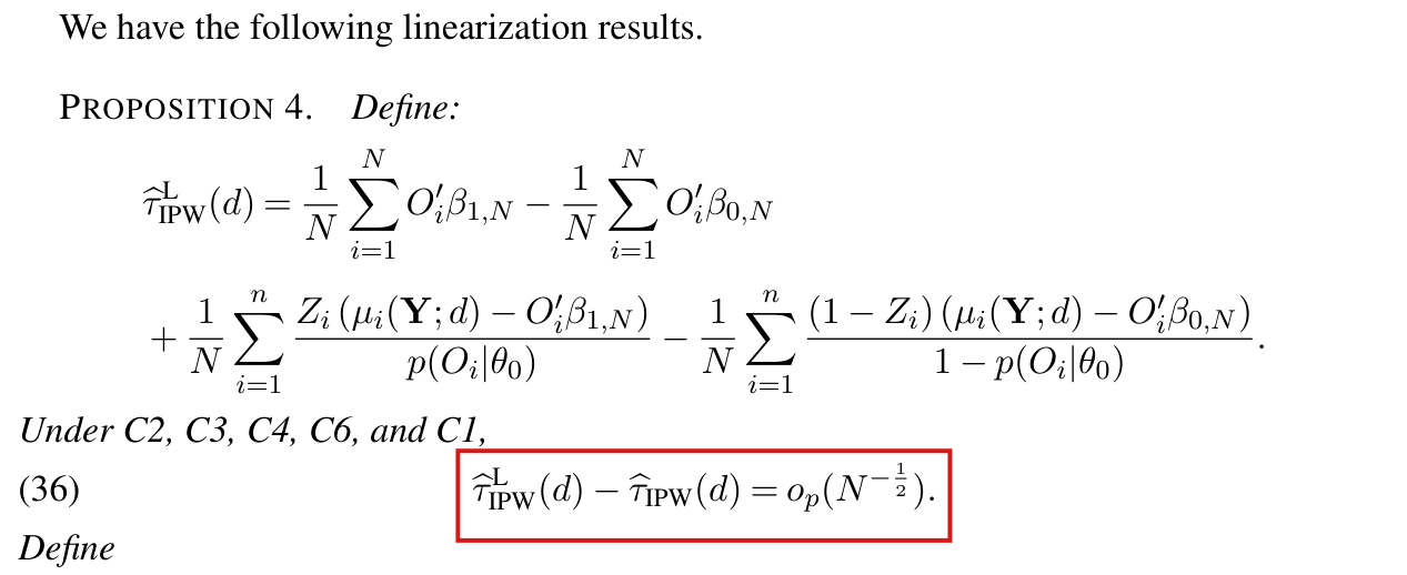
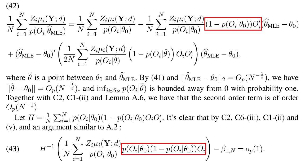
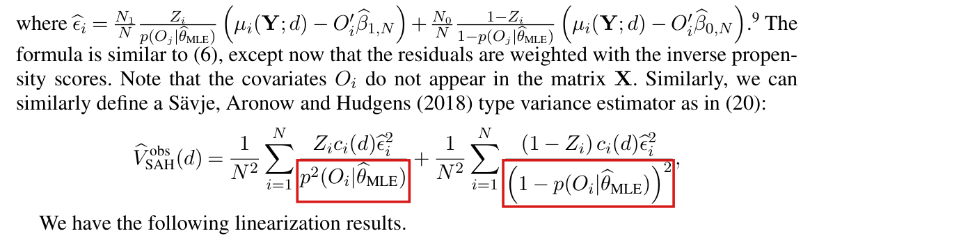
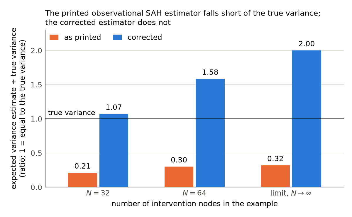
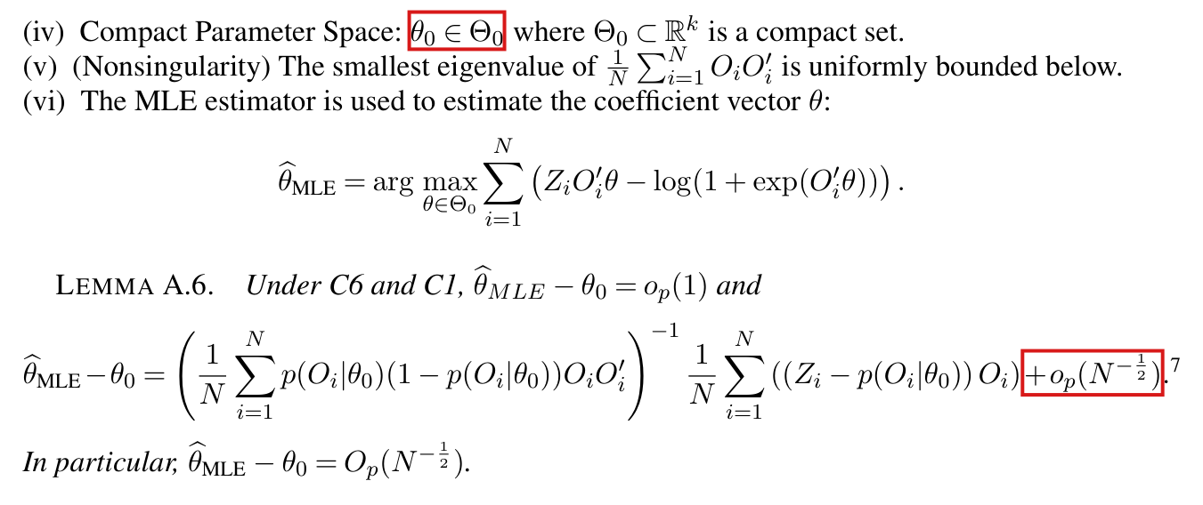
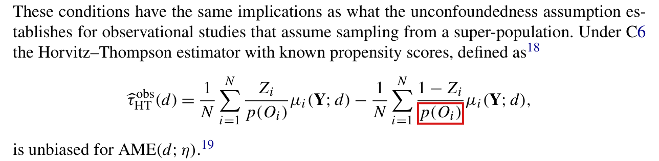
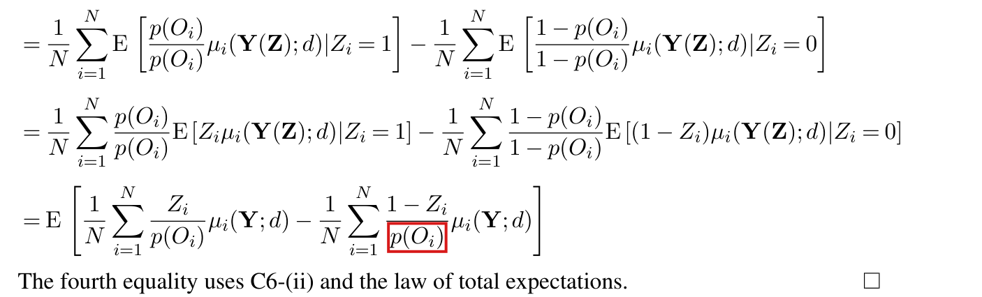
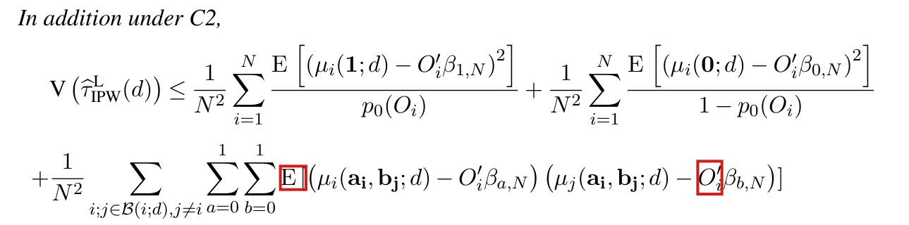
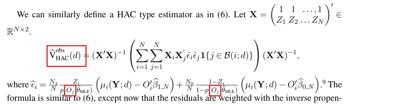
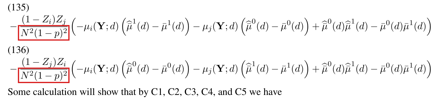
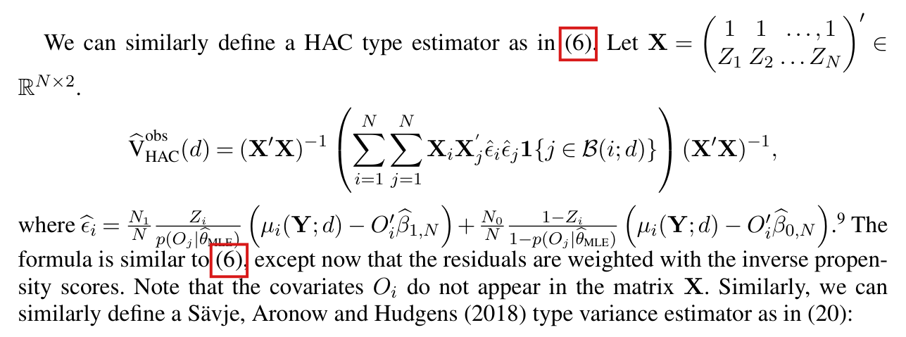
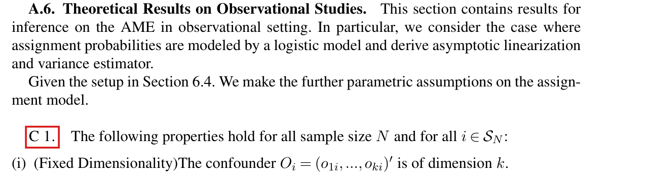
(S7) Observational setting [Section 6.4, p. 758 (PDF p. 15); Supplement A.6, pp. 13-15]. 'we denote a vector of confounder attributes for intervention node $i$ as $O_i$ and make the following independent assignment assumption: C6 (Probablistic Assignment). For all sample sizes $N$: (i) The random assignment variables $\{Z_i\}_{i=1}^N$ are jointly independent. (ii) There exists a treatment probability model $p(\cdot):\mathcal O\to[0,1]$ such that, for each $i\in\mathcal S_N$, (30) $\mathbf{Prob}(Z_i=1)=p(O_i)$. (iii) For an $\epsilon\in(0,\frac12)$ and for all $i\in\mathcal S_N$, $\mathbf{Prob}(Z_i=1)\in(\epsilon,1-\epsilon)$.' Footnote 19 (p. 759): 'Note that the AME is defined by marginalizing over the independently but not identically distributed assignment variables generated by the assignment mechanism.' Supplement A.6 (pp. 13-14): 'C 1. The following properties hold for all sample size $N$ and for all $i\in\mathcal S_N$: (i) (Fixed Dimensionality)The confounder $O_i=(o_{1i},...,o_{ki})'$ is of dimension $k$. (ii) (Bounded Confounders) Confouders are uniformly bounded: there exists a constant $U$ such that $\max_{i\in\mathcal S_N}||O_i||_\infty\le U$. (iii) (Logistic Model) The assignment probabilites follow a logistic model: for all $i\in\mathcal S_N$ there exists a $\theta_0\in\mathbb R^k$ such that $P(Z_i=1)=p(O_i|\theta)=\frac{\exp(O_i'\theta_0)}{1+\exp(O_i'\theta_0)}$ (iv) Compact Parameter Space: $\theta_0\in\Theta_0$ where $\Theta_0\subset\mathbb R^k$ is a compact set. (v) (Nonsingularity) The smallest eigenvalue of $\frac1N\sum_{i=1}^NO_iO_i'$ is uniformly bounded below. (vi) The MLE estimator is used to estimate the coefficient vector $\theta$: $\hat\theta_{\mathrm{MLE}}=\arg\max_{\theta\in\Theta_0}\sum_{i=1}^N\big(Z_iO_i'\theta-\log(1+\exp(O_i'\theta))\big)$.' 'We defined the following IPW estimator: $\hat\tau_{\mathrm{IPW}}(d)=\frac1N\sum_{i=1}^N\frac{Z_i}{p(O_i|\hat\theta_{\mathrm{MLE}})}\mu_i(\mathbf Y;d)-\frac1N\sum_{i=1}^N\frac{1-Z_i}{1-p(O_i|\hat\theta_{\mathrm{MLE}})}\mu_i(\mathbf Y;d)$. For brevity, we denote $p(O_i|\theta_0)=p_0(O_i)$. We define the following coefficients: $\beta_{1,N}=\Big(\frac1N\sum_{i=1}^Np_0(O_i)(1-p_0(O_i))O_iO_i'\Big)^{-1}\Big(\frac1N\sum_{i=1}^N\mathrm E[\mu_i(1;d)p_0(O_i)(1-p_0(O_i))O_i]\Big)$, and, $\beta_{0,N}=\Big(\frac1N\sum_{i=1}^Np_0(O_i)(1-p_0(O_i))O_iO_i'\Big)^{-1}\Big(\frac1N\sum_{i=1}^N\mathrm E[\mu_i(0;d)p_0(O_i)(1-p_0(O_i))O_i]\Big)$.' 'C 2. For all sample size $N$, $\frac1N\sum_{i=1}^N\big(\tau_i(d;\eta)-(O_i'\beta_{1,N}-O_i'\beta_{0,N})\big)\sum_{j\in\mathcal B(i;d)}\big(\tau_j(d;\eta)-(O_i'\beta_{1,N}-O_i'\beta_{0,N})\big)\ge0$.' (p. 15) '$\hat{\mathrm V}^{\mathrm{obs}}_{\mathrm{HAC}}(d)=(\mathbf X'\mathbf X)^{-1}\Big(\sum_{i=1}^N\sum_{j=1}^N\mathbf X_i\mathbf X_j'\hat\epsilon_i\hat\epsilon_j\mathbf 1\{j\in\mathcal B(i;d)\}\Big)(\mathbf X'\mathbf X)^{-1}$, where $\hat\epsilon_i=\frac{N_1}N\frac{Z_i}{p(O_j|\hat\theta_{\mathrm{MLE}})}\big(\mu_i(\mathbf Y;d)-O_i'\hat\beta_{1,N}\big)+\frac{N_0}N\frac{1-Z_i}{1-p(O_j|\hat\theta_{\mathrm{MLE}})}\big(\mu_i(\mathbf Y;d)-O_i'\hat\beta_{0,N}\big)$', with footnote 9: '$\hat\beta_{1,N}=\Big(\frac1N\sum_{i=1}^Np(O_i|\hat\theta_{\mathrm{MLE}})(1-p(O_i|\hat\theta_{\mathrm{MLE}}))O_iO_i'\Big)^{-1}\Big(\frac1N\sum_{i=1}^N\frac{Z_i\mu_i(\mathbf Y;d)}{p(O_i|\hat\theta_{\mathrm{MLE}})}p(O_i|\hat\theta_{\mathrm{MLE}})(1-p(O_i|\hat\theta_{\mathrm{MLE}}))O_i\Big)$ and $\hat\beta_{0,N}=\Big(\frac1N\sum_{i=1}^Np(O_i|\hat\theta_{\mathrm{MLE}})(1-p(O_i|\hat\theta_{\mathrm{MLE}}))O_iO_i'\Big)^{-1}\Big(\frac1N\sum_{i=1}^N\frac{(1-Z_i)\mu_i(\mathbf Y;d)}{1-p(O_i|\hat\theta_{\mathrm{MLE}})}p(O_i|\hat\theta_{\mathrm{MLE}})(1-p(O_i|\hat\theta_{\mathrm{MLE}}))O_i\Big)$'; and '$\hat V^{\mathrm{obs}}_{\mathrm{SAH}}(d)=\frac1{N^2}\sum_{i=1}^N\frac{Z_ic_i(d)\hat\epsilon_i^2}{p^2(O_i|\hat\theta_{\mathrm{MLE}})}+\frac1{N^2}\sum_{i=1}^N\frac{(1-Z_i)c_i(d)\hat\epsilon_i^2}{(1-p(O_i|\hat\theta_{\mathrm{MLE}}))^2}$'.
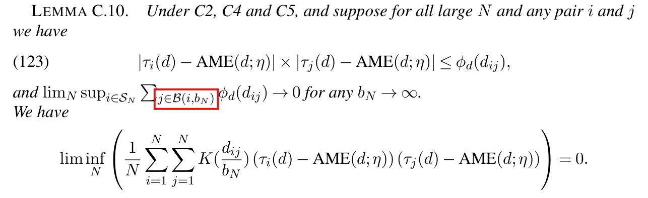
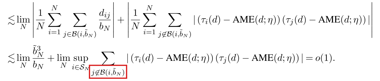
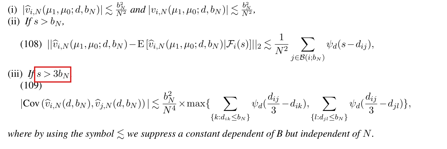
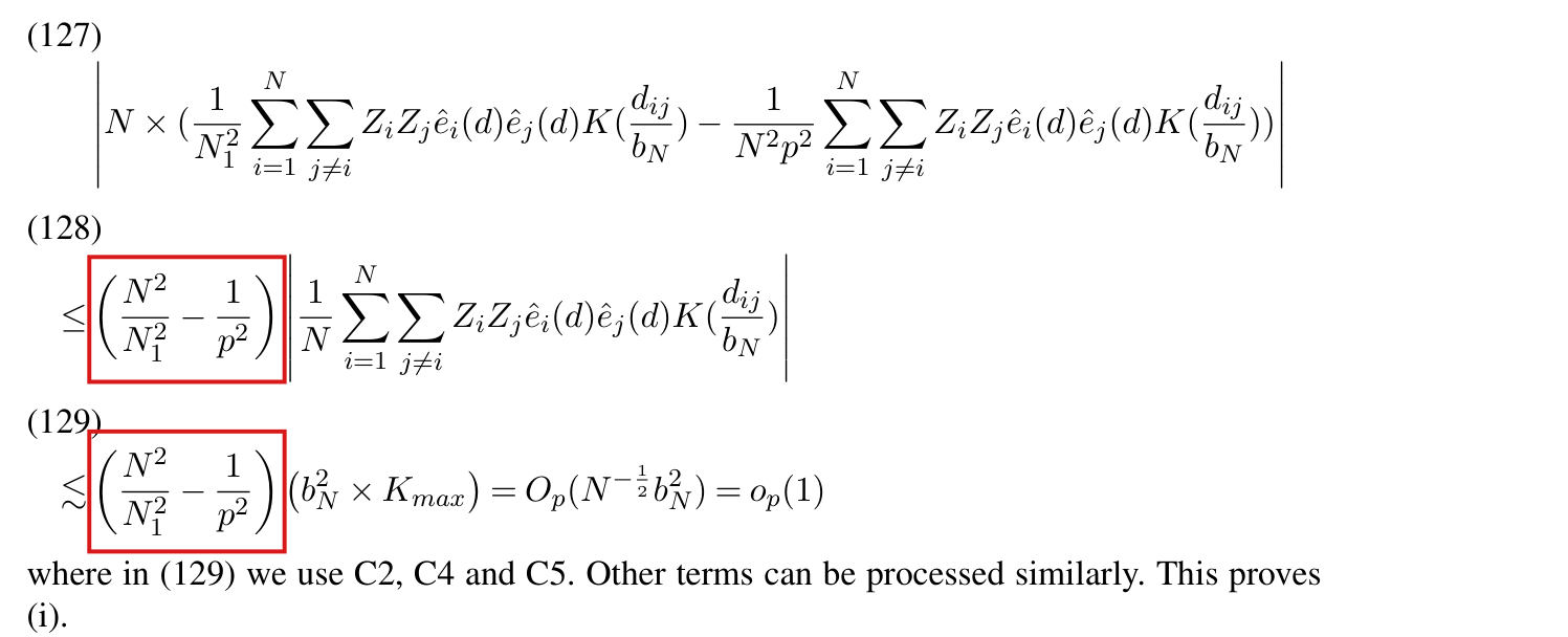
(S8) Near-epoch dependence [Supplement A, Appendix C, pp. 25-34]. 'Let $\mathcal S_N$ be a set of intervention nodes equipped with a distance metric $\gamma$ that satisfies positivity and the triangle inequality. Let $H_N=\{H_{i,N},i\in\mathcal S_N\}$ and $V_N=\{V_{i,N},i\in\mathcal S_N\}$ be two arbitrary sets of random variables. Define $\mathcal F_i(s)=\sigma(V_{j,N},j\in\mathcal S_n,\gamma(i,j)\le s)$ ... Denote the $L_p$-norm of a random variable as $||X||_p=(E[|X|^p])^{\frac1p}$.' 'Definition 1 ($L_2$-NED). Let $H_N=\{H_{i,N},i\in\mathcal S_N,N\ge1\}$ be a random field with $||H_{i,N}||_2<\infty$. Let $V_N=\{V_{i,N},i\in\mathcal S_N,N\ge1\}$ be a random field, where $|\mathcal S_N|=N$, and let $g_N=\{g_{i,N},i\in\mathcal S_N,N\ge1\}$ be a set of positive constants. Then the random field $H_N$ is said to be $L_2(g_N)$-near-epoch dependent on the random field $V_N$ if, for all $i$, (51) $||H_{i,N}-\mathrm E[H_{i,N}|\mathcal F_{i,N}(s)]||_2\le g_{i,N}\psi(s)$, for a non-increasing sequence $\psi(s)\ge0$ with $\lim_{s\to\infty}\psi(s)=0$. $H_N$ is said to be $L_2$-NED on $V_N$ of size $-\lambda$ if $\psi(s)=O(s^{-\mu})$ for some $\mu>\lambda>0$. Further more, if $\sup_N\sup_{i\in\mathcal S_N}g_{i,N}<\infty$, then $H_N$ is said to be uniformly $L_2$-NED on $V_N$.' 'Let $\mathcal F_i^c(s)=\sigma(V_{j,N},j\in\mathcal S_n,\gamma(i,j)>s)$'. (p. 26) 'We shall inherit C1 and C2. We relax C3 with the following weak-dependence assumption. C 3. For any $d$-circle average outcomes and for all sample sizes, $\{\mu_i(\mathbf Y,d),i\in\mathcal S_N\}$ is uniform $L_2$-NED of size -4 on the random field $\{Z_i,i\in\mathcal S_N\}$.' 'Denote the corresponding NED-coefficient function as $\psi_d():\mathbb R_+\to\mathbb R_+$.' (p. 27) 'C 4. For each radius $s\ge0$ and all large sample sizes $N$, there exists a $C_b>0$ such that $\sup_{i\in\mathcal S_N}|\mathcal B_N(i;s)|\le b(s)$, with $b(s)=C_bs^2$.' [In Appendix C, $\mathcal B_N(i;s)$ is the set of nodes within distance $s$ of $i$.] (p. 32) 'C 5. The kernel function $K:\mathbb R_+\to\mathbb R$ has the following properties: 1. $K(0)=1$. 2. It is supported on $[0,1]$. 3. It is uniformly bounded: there exists a $K_{max}<\infty$ such that $\sup_{x\in\mathbb R_+}|K(x)|<K_{max}$. 4. It is locally Lipschitz at 0: there exists a $\epsilon\in(0,1)$ and a positive constant $C>0$ such that (101) $|K(x)-1|\le C|x|$, for any $x\in[0,\epsilon)$.' Footnote 19: 'This means that $K(x)=0$ for all $x>1$.' '(102) $\hat\epsilon_{i,N}(\mu_1,\mu_0;d)=\frac{\mathbf Z_i}{Np}(\mu_i(\mathbf Y;d)-\mu_1)-\frac{1-\mathbf Z_i}{N(1-p)}(\mu_i(\mathbf Y;d)-\mu_0)$.' '(107) $\hat v_{i,N}(\mu_1,\mu_0;d,b_N)=\sum_{j\in\mathcal B(i;b_N)}\hat\epsilon_{i,N}(\mu_1,\mu_0;d)\hat\epsilon_{j,N}(\mu_1,\mu_0;d)K(\frac{d_{ij}}{b_N})$, and $v_{i,N}(\mu_1,\mu_0;d,b_N)=\mathrm E[\hat v_{i,N}(\mu_1,\mu_0;d,b_N)]$'. (p. 34) 'C 6. Given a kernel function $K$ and a sequence of bandwidth $\{b_N\}_{N=1}^\infty$, (122) $\liminf_N\Big(\frac1N\sum_{i=1}^N\sum_{j=1}^NK(\frac{d_{ij}}{b_N})(\tau_i(d)-\mathrm{AME}(d;\eta))(\tau_j(d)-\mathrm{AME}(d;\eta))\Big)\ge0$.' Footnote 20: 'Note if $b_N$ is fixed and $K$ is the uniform kernel, this reduces to C5.'
(S9) Label collisions (a reader's note, not the paper's text). Supplement A reuses the labels of the article for different statements: 'C 1' and 'C 2' of Supplement A.6 are the logistic-model block and a homophily condition of (S7), not C1 and C2 of (S4); 'C 3' to 'C 6' of Appendix C are the conditions of (S8), not C3-C6 of (S4), (S5) and (S7); and Supplement A has its own Propositions 1-6 (A.4.1 Proposition 1, A.4.2 Proposition 2, A.5 Proposition 3, A.6 Proposition 4, Appendix C Propositions 5 and 6), distinct from Propositions 1-4 of the article. Every target below says which is meant. In Supplement A.6 the hypothesis list 'Under C2, C3, C4, C6, and C1' means C2-C4 of (S4), C6 of (S7) and 'C 1' of Supplement A.6; 'additionally under C2' in items (i)-(ii) of its Proposition 4 means 'C 2' of Supplement A.6.
Effective claim (source TeX): Printed statement refuted. Supplement A p. 15: 'Proposition 4. Define: $\hat\tau^{\mathrm L}_{\mathrm{IPW}}(d)=\frac1N\sum_{i=1}^NO_i'\beta_{1,N}-\frac1N\sum_{i=1}^NO_i'\beta_{0,N}+\frac1N\sum_{i=1}^n\frac{Z_i(\mu_i(\mathbf Y;d)-O_i'\beta_{1,N})}{p(O_i|\theta_0)}-\frac1N\sum_{i=1}^n\frac{(1-Z_i)(\mu_i(\mathbf Y;d)-O_i'\beta_{0,N})}{1-p(O_i|\theta_0)}$. Under C2, C3, C4, C6, and C1, (36) $\hat\tau^{\mathrm L}_{\mathrm{IPW}}(d)-\hat\tau_{\mathrm{IPW}}(d)=o_p(N^{-\frac12})$.' (The two upper limits printed $n$ are read as $N$; 'C1' is 'C 1' of Supplement A.6, see (S9).)
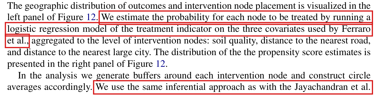
Witness (validators; exact). For each integer $K\ge1$ let $N=3K$. Node $i\in\{1,\ldots,N\}$ is the point $(10i,0)$ of the plane with Euclidean distance, and has type $t(i)\in\{-1,0,1\}$, the types repeating in the cyclic order $-1,0,1$. The outcome points are the node points, $\zeta$ is counting measure, $\Omega_d=[0,d]$, and the distance audited is $d=0$, so $\mu_i(\mathbf Y(\mathbf z);0)=Y_{(10i,0)}(\mathbf z)$. For every $\mathbf z\in\{0,1\}^N$, $Y_{(10i,0)}(\mathbf z)=q_{t(i)}$ with $q_{-1}=1$, $q_0=\frac{21}{20}$, $q_1=1$. Confounders $O_i=(1,t(i))'$, $\theta_0=(0,\log2)'$, $\Theta_0=[-2,2]^2$; the $Z_i$ are independent with $\Pr(Z_i=1)=p_{t(i)}=\frac{2^{t}}{1+2^{t}}$, that is $(p_{-1},p_0,p_1)=(\frac13,\frac12,\frac23)$. Write $w_t=p_t(1-p_t)=(\frac29,\frac14,\frac29)$.
(W1) Every hypothesis of the proposition holds, and so do the further conditions the paper uses later: C2 with $b=2$; no assignment changes any outcome, so $s_{ij}(0)=0$ for $i\ne j$, C3 holds with $h(0)=0$, $\mathcal B(i;0)=\{i\}$ and $c_i(0)=1$; C4 holds because nodes are 10 apart; C6 holds with $\epsilon=\frac1{10}$; 'C 1' of Supplement A.6 holds with $k=2$, $U=1$, $\frac1N\sum_iO_iO_i'=\mathrm{diag}(1,\frac23)$, and $\theta_0$ is an interior point of $\Theta_0$ since $0<\log2<1$; $\tau_i(0;\eta)=0$ for all $i$ and $\beta_{1,N}=\beta_{0,N}$, so the left side of 'C 2' is $0$ in the printed form and in the form with $O_j$; and $N\,\mathrm V(\hat\tau^{\mathrm L}_{\mathrm{IPW}}(0))=\frac{1753}{750000}>0$ (the printed nondegeneracy proviso).
(W2) Exact constants. $H_N=\frac1N\sum_ip_i(1-p_i)O_iO_i'=\mathrm{diag}(\frac{25}{108},\frac4{27})$; $\beta_{1,N}=\beta_{0,N}=(\frac{509}{500},0)'$; $D_N=\frac1N\sum_i[(1-p_i)m_{i1}+p_im_{i0}]O_i=(\frac{61}{60},0)'$ where $m_{ia}=\mathrm E[\mu_i(\mathbf a;0)]=q_{t(i)}$; $\gamma_N=H_N^{-1}D_N=(\frac{549}{125},0)'$; $\mathrm{AME}(0;\eta)=0$.
(W3) For every assignment, the printed linearization is $\hat\tau^{\mathrm L}_{\mathrm{IPW}}(0)=\frac1N\sum_ib_{t(i)}(Z_i-p_{t(i)})$ with $b_t=\frac{q_t-O_t'\beta_{1,N}}{p_t(1-p_t)}$, $(b_{-1},b_0,b_1)=(-\frac{81}{1000},\frac{16}{125},-\frac{81}{1000})$; and the first-order form of the IPW estimator is $\hat\tau^{\mathrm{true}}_{\mathrm{HT}}-\frac1N\sum_i(Z_i-p_i)O_i'\gamma_N=\frac1N\sum_ia_{t(i)}(Z_i-p_{t(i)})$ with $a_t=\frac{q_t}{p_t(1-p_t)}-O_t'\gamma_N$, $(a_{-1},a_0,a_1)=(\frac{27}{250},-\frac{24}{125},\frac{27}{250})$, where $\hat\tau^{\mathrm{true}}_{\mathrm{HT}}=\frac1N\sum_i[\frac{Z_i\mu_i}{p_i}-\frac{(1-Z_i)\mu_i}{1-p_i}]$. So $a_t-b_t=(\frac{189}{1000},-\frac{8}{25},\frac{189}{1000})$.
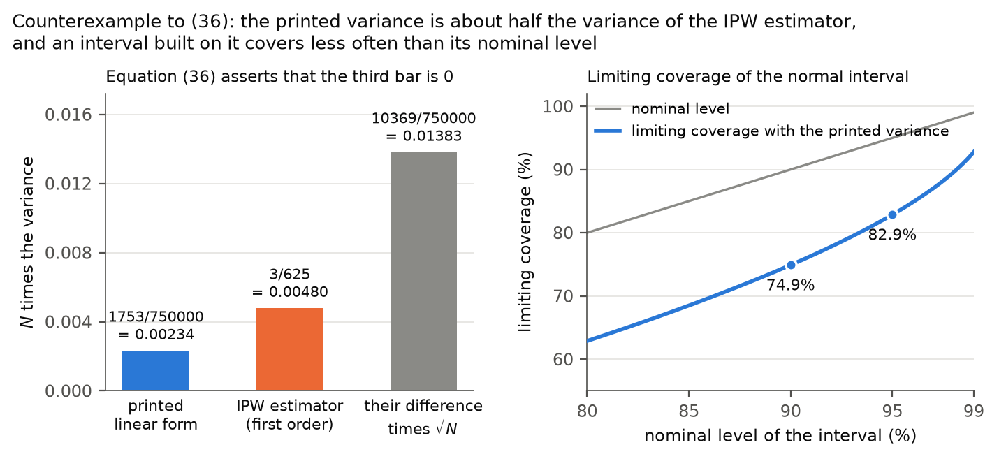
(W4) $N$-scaled variances: $V_A=\frac13\sum_tw_ta_t^2=\frac3{625}$, $V_P=\frac13\sum_tw_tb_t^2=\frac{1753}{750000}$, $V_D=\frac13\sum_tw_t(a_t-b_t)^2=\frac{10369}{750000}$.
(W5) Let $B_j=\sum_{t\in\{-1,0,1\}}(a_t-b_t)(Z_{j,t}-p_t)$ be the sum over the three nodes of block $j$, and $U_K=(3K)^{-1/2}\sum_{j=1}^KB_j$. The $B_j$ are i.i.d., $\mathrm E[B_j]=0$, $\mathrm E[B_j^2]=3V_D$, $\mathrm E[B_j^4]=\frac{915255049}{250000000000}$. For every $K\ge1$: $\mathrm E[U_K^2]=V_D$, $\mathrm E[U_K^4]=\frac{\mathrm E[B_j^4]}{9K}+\frac{3(K-1)V_D^2}{K}\le\frac{2205448981}{2250000000000}$, and therefore $\Pr\big(U_K^2>\frac{V_D}2\big)\ge\frac{V_D^2}{4\cdot\frac{2205448981}{2250000000000}}=\frac{107516161}{2205448981}>0$.
(W6) Conclusion. $\hat\tau_{\mathrm{IPW}}(0)=\frac1N\sum_ia_{t(i)}(Z_i-p_{t(i)})+O_p(N^{-1})$, hence $\sqrt N\big(\hat\tau_{\mathrm{IPW}}(0)-\hat\tau^{\mathrm L}_{\mathrm{IPW}}(0)\big)=U_K+o_p(1)$, and by (W5) it does not converge to $0$ in probability: (36) fails. Moreover $\sqrt N\,\hat\tau_{\mathrm{IPW}}(0)\Rightarrow\mathcal N(0,\frac3{625})$ while $N\,\mathrm V(\hat\tau^{\mathrm L}_{\mathrm{IPW}}(0))=\frac{1753}{750000}$, so the ratio standardized as on Supplement A p. 16 has limiting variance $\frac{V_A}{V_P}=\frac{3600}{1753}\ne1$, and a normal interval built on a variance estimate that is consistent for $V_P/N$ has limiting coverage $2\Phi\big(z_{1-\alpha/2}\sqrt{1753/3600}\big)-1<1-\alpha$.
: SAP.P004a.T1WholeStatement
Theorem: SAP.P004a.T1
Statement hash: 85ecf863c123df1f43c7dd7690c58764741d0544d12b0882a3c2d7fd8bea69ba
Statement definition: SAP.P004a.T1WholeStatement
Certificate. 20261104T212927Z
Declaration review: faithful; 2026-11-04T21:56:29Z; binding v2
Evidence scope: Certification checks formal proof objects. Statement fidelity is a model judgment. Author review is separate.
Proof dependencies: Independently extracted
Manifest annotation reconciliation: Effective use follows the source-bound dependency observation; original annotations are retained in the crosswalk.
AronowAudit.P004.Wave1.ipw_linearization_counterexample_nat: observed not used
AronowAudit.P004.ipw_witness_variance_constants: observed not used
Source and evidence metadata · sap-2026-11-08-assured-release