LLM-generated corrections to the published research of P. M. Aronow

Journal article P008

Corrections to: Inference in Spatial Experiments with Interference using the SpatialEffect Package

Cyrus Samii, Ye Wang, Jonathan Sullivan, and P. M. Aronow (2023). Inference in Spatial Experiments with Interference using the SpatialEffect Package. Journal of Agricultural, Biological, and Environmental Statistics 28(1):138–156.

DOI
10.1007/s13253-022-00517-y
arXiv
2106.15081
Audited edition
Journal of Agricultural, Biological, and Environmental Statistics, 2023, 28(1):138–156; 19 pages in the audited file
SHA-256 of the audited file
97f8e362d0e220b15805eaf7e835ea80dfe3f158d3fef954746b652083c5fa9f
Permanent address
https://pmaronow.github.io/llm-audit/works/P008/

Summary

This tutorial presents design-based inference for spatial experiments with interference. It targets the average marginalized response (AMR), the average effect of treating a node on points at distance dd, and estimates it with the SpatialEffect package. An application to a forest-conservation experiment in Uganda reports spillovers up to 2.5 km. 21 entries are classified as errors (1 Major, 3 Moderate, 17 Minor), and 1 is a clarity note. In the Major one, P008-N012, the displayed procedure defaults to unrestricted permutations over 121 villages, which do not follow the experiment’s lotteries, so its significance at the 5% level is not established.

What was and was not checked

I checked the following points, which held up within the limits stated here.

  • Section 2.2: the marginalization over the other nodes, the exchange of the expectation with the circle average, and the identity for the AMR once its display is corrected as in P008-E005. With additive effects and Bernoulli assignment, the effect τix\tau_{ix} equals the additive effect of node ii in the toy example.
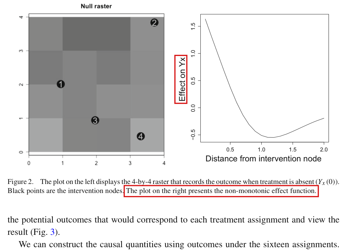
  • Figure 4: the true AMR of the toy example agrees with the AMR computed from the definition over the 16 Bernoulli assignments, with a largest difference below 0.0001 against the curve read from the figure. At d=0.35d=0.35 the circle around node 1 crosses four raster cells and that around node 2 crosses one (p. 147).
  • The output on p. 149: the ten estimates and the twenty permutation bounds are reproduced from the seed of the vignette, and the twenty endpoints of the spatial-HAC intervals by a node-level calculation with cutoff 0.4. What those intervals mean is the subject of P008-N002. Figure 5 agrees with the recalculation at all 20 radii, apart from the smoothed curve, which was not reproduced (P008-N007).
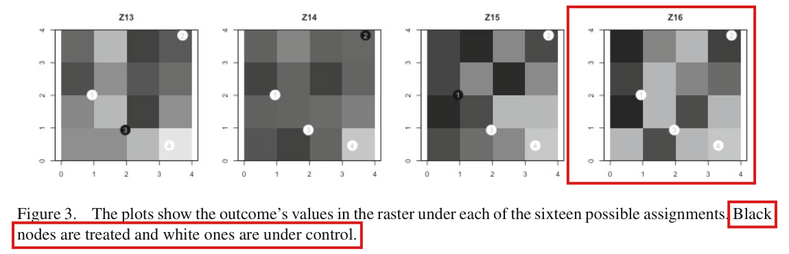
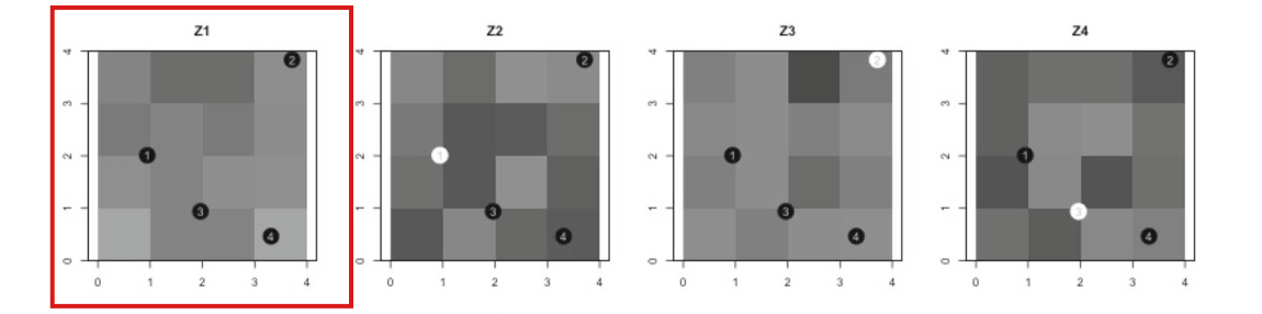
  • Footnote 5: there are exactly six assignments with two of the four nodes treated. The bounds −7.97-7.97 and 7.977.97 on p. 149 are the rounded default quantiles of the six statistics. Their use for a test at the 5% level is the subject of P008-E002.
  • The Hajek estimator on p. 144 is what both archived versions of the package compute, a difference in means of circle averages. The weak null is implied by the sharp null and not conversely (p. 144).
  • Figure 8, panel of the Hajek estimator: the estimates at 0 to 3.5 km are reproduced within 0.0004, and the cumulative statistic as −0.0322-0.0322 against the printed −0.0321-0.0321, from a forest-loss raster and digitized polygons archived with later replication files. These are not established to be the inputs of the tutorial. The eleven estimates of the bottom panel agree with a calculation from later replication inputs with a root mean square difference of 0.0000521 when indexed by each band’s outer radius. Where they are drawn is the subject of P008-N017.
  • p. 151 and Figure 6: 121 villages, 60 treated and 61 control. The take-up of 32% and the compliance of 88% are consistent with the source study’s posted data, and the two spillover checks attributed to Jayachandran et al. (2017) match that study’s code.
  • p. 153: 20/111≈0.1820/111\approx0.18 and 5/111≈0.0455/111\approx0.045 as arithmetic (the step itself is the subject of P008-E004), 1010 km =10,000=10{,}000 m, and the comparison −0.0321<−0.0304-0.0321<-0.0304.

I did not check the consistency and asymptotic normality of the estimator or the conservativeness of the intervals against the proofs in Wang et al. (2022), to which the tutorial attributes these results. I checked the quoted background facts for Jayachandran et al. (2017) against the posted data and code, and the assignment restrictions discussed in P008-N012 against its Supplementary Materials. I could not reproduce the original application, since the release that the paper cites (version 0.1), a script for Figure 8 and the transformed inputs are not archived. The findings about code concern the two archived versions of the package, neither of which is that release. Twelve large files of the source study’s deposit and most simulation scripts of the later replication files were not read. The circle averages of the application’s edge estimates beyond 3.5 km and its smoothed curve, which is calibrated by cross-validation, were not recomputed.
The paper has no appendix; no official supplement or correction to it was available, and I read all 19 pages. Where this list or the corrections are silent about a passage, the silence is not a finding that the passage is correct.

Headline claims and related corrections

  1. The target quantity is the average marginalized response (AMR): the average effect, on points at distance dd from an intervention node, of activating treatment at that node, marginalizing over the treatment of the other nodes under the design.

    Section 2.2, the displays defining Yix(z;α)Y_{ix}(z;\alpha), τix(α)\tau_{ix}(\alpha), μi\mu_i and τ(d;α)\tau(d;\alpha); Figure 4 (true AMR of the toy example)

    See P008-E005, P008-E007.

  2. The AMR is estimated by a simple design-based (Hajek) contrast of circle averages, which is consistent and asymptotically normal under mild conditions (attributed to Wang et al. 2022) and supports two kinds of inference without a parametric outcome model: a sharp-null permutation test and normal intervals with a spatial-HAC standard error.

    Section 2.3 displayed Hajek estimator and inferential prescriptions (pp. 143-145); Section 3 (pp. 145-146); Figure 5; Wang et al. (2022) for the asymptotic results

    See P008-E002, P008-N002.

  3. The toy example with four nodes illustrates a non-monotonic effect and an estimated AMR whose shape corresponds to the true AMR, and concludes that the sharp null of no cumulative effect on [0.1,0.5][0.1,0.5] is rejected at the 5% level.

    Sections 4-5 (pp. 146-150); Figures 2-5; printed output table on p. 149; footnote 5

    See P008-E002, P008-E003, P008-E006, P008-E015, P008-N001, P008-N004, P008-N005, P008-N006, P008-N007.

  4. The application to the Uganda payments-for-conservation experiment reports a cumulative effect on forest loss of −0.0321-0.0321 between 1 and 2.5 km, with p<0.05p<0.05, and interprets it as positive conservation spillovers reaching up to 2.5 km.

    Section 6 (pp. 153–154); Figure 8; output of SpatialEffectTest() quoted on p. 153 (−0.0321-0.0321; percentiles −0.0304-0.0304 and 0.03360.0336); abstract, p. 139; conclusion, p. 155

    See P008-E004, P008-E009, P008-E012, P008-N009, P008-N012, P008-N016, P008-N017.

  5. The spillovers imply that the original between-village comparison may have understated the overall impact of the program.

    p. 154 and conclusion p. 155; rests on Figure 8 and the cumulative test of Section 6

    See P008-N016.

  6. When effects are additive or homogeneous the AMR equals the spillover coefficient of a linear structural model, and it keeps a meaningful interpretation under heterogeneous and nonadditive responses (attributed to Wang et al. 2022).

    p. 140; Wang et al. (2022); no numbered result in this paper

  7. Linear functionals of the AMR (sums or means over a range of distances) characterize cumulative spatial responses and can be tested by permutation with SpatialEffectTest().

    p. 140; Section 3 description of SpatialEffectTest() (p. 146); toy cumulative output (pp. 149-150); Uganda cumulative output (p. 153)

    See P008-E002, P008-E003, P008-E004, P008-N016.

  8. The SpatialEffect package provides a practical step-by-step implementation for point or polygon interventions and raster or point outcomes, with permutation, spatial-HAC and smoothed estimates.

    Abstract; Section 3 package features; Section 5 tutorial and Figure 5; Section 6 tutorial and Figure 8; conclusion p. 155

    See P008-E004, P008-E006, P008-E009, P008-E012, P008-E015, P008-N001, P008-N006, P008-N007.

Corrections

Major (1)

A central result, method or key claim fails for a non-trivial reason, and the repair changes what the paper establishes.

The statement “significant with p<0.05p < 0.05” is not established under the design of the experiment: in the inspected implementations, the printed call permutes treatment freely over the 121 villages, but treatment was assigned by seven subcounty lotteries between lists of villages balanced on covariates.

Section 6, displayed SpatialEffect() call and the paragraph after the SpatialEffectTest() call, p. 153 (PDF p. 16); see also p. 151 (PDF p. 14) and p. 145 (PDF p. 8)

See also under Formal statements (Lean): P008-T1, P008-T2, P008-T4, P008-T21

My comment on this entry

As printed

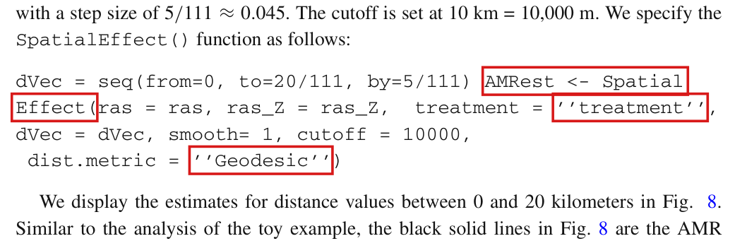
dVec = seq(from=0, to=20/111, by=5/111) AMRest <- Spatial

Effect(ras = ras, ras_Z = ras_Z, treatment = ’’treatment’’,

dVec = dVec, smooth= 1, cutoff = 10000,

dist.metric = ’’Geodesic’’)

testResult <- SpatialEffectTest(AMRest, test.range = c(1/111,

2.5/111))

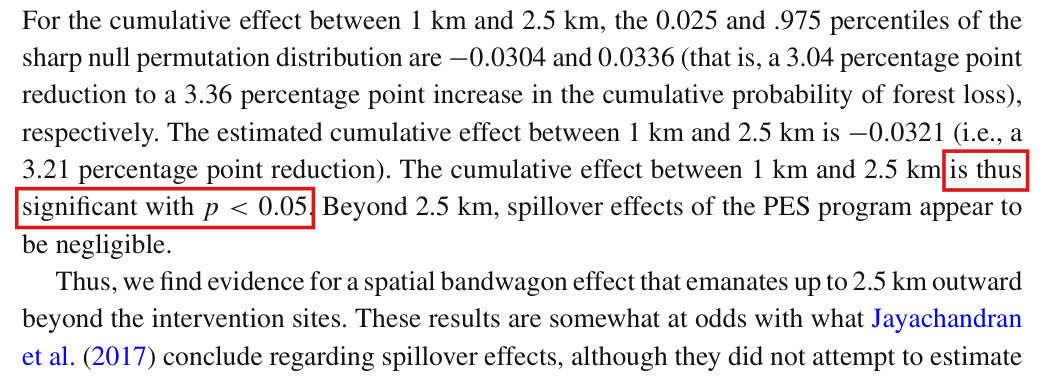
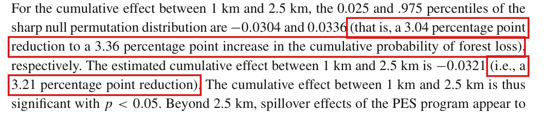
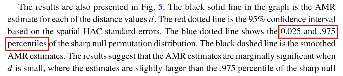
For the cumulative effect between 1 km and 2.5 km, the 0.025 and .975 percentiles of the sharp null permutation distribution are −0.0304-0.0304 and 0.03360.0336 […], respectively. The estimated cumulative effect between 1 km and 2.5 km is −0.0321-0.0321 […]. The cumulative effect between 1 km and 2.5 km is thus significant with p<0.05p < 0.05.

[p. 151] The study was carried out in 121 villages, 60 of which were randomly assigned to treatment (Fig. 6).

The problem

The paper takes the distribution of the treatment assignment as known and derives its inference from that distribution (p. 142). It also says that the permutation test can be adjusted for blocking or clustering in the design (p. 145). The printed call for the application passes neither blockvar nor clustvar. With these defaults, the inspected implementations draw the permutations uniformly from the assignments that treat 60 of the 121 villages.

The experiment was not randomized in this way. According to the Supplementary Materials of the source study (Jayachandran et al., 2017, section 2.2), treatment was assigned by a public lottery in each of seven subcounties. Before each lottery the sample villages of the subcounty were divided into two lists. The sizes of the two lists differ by at most one, and the lists are balanced on four village covariates (the number of forest owners sampled, distance to a road, income per capita and landholding size), with a threshold of 0.25 on each standardized mean difference. In small subcounties all partitions were examined, and in larger ones 1000 were sampled. One eligible partition was selected at random before each public draw, and the lottery chose between its two lists. This is neither an unrestricted choice of 60 villages nor an independent assignment of each village. Conditioning on the total of 60 treated villages does not remove the subcounty and balance restrictions.

The assignment in the source experiment and the printed call’s inspected defaults.
Source experimentPrinted call
Assignment groupsseven subcountiesall 121 villages together
What is drawnone of two lists of villages60 of the 121 villages
Balance on covariatesrequired of the two listsnone

The unrestricted default does not generate the randomization distribution of the experiment. The reported rejection rests on a margin of 0.00170.0017, between −0.0321-0.0321 and −0.0304-0.0304, and does not establish significance at the 5% level under the design. This is the only formal test in the application. The restrictions also rule out independent assignment of the 121 villages, so a justification of the spatial-HAC intervals that relies on Bernoulli assignment needs a further argument for this design.

Evidence a derivation

I base this correction on the published protocol of the source study, the displayed call and an exact derivation. The protocol is quoted from the copy of the Supplementary Materials posted by the first author of the source study (Materials and Methods, section 2.2, p. 3). It refers to “each of the 7 subcounties” and says that, in advance of each lottery, the sample villages in the subcounty were divided “into two sets, balanced on covariates”. The printed call shows no blocking or clustering argument. In both inspected implementations, these arguments default to NULL and are passed to the permutation routine of the ri package, which then draws uniformly among the assignments with the observed number of treated units. I could not reconstruct the published computation, since I do not have the cited package release or the original application code.
Neither the size nor the direction of the change can be inferred without recomputing the test. Let four units be given, two of them treated, and let the statistic be the difference in means at the assignment (1,0,1,0)(1,0,1,0). With fixed outcomes (0,1,0,1)(0,1,0,1), the two-sided tail probability is 1/31/3 under free permutation and 1/21/2 when one unit is treated in each of the pairs {1,2}\{1,2\} and {3,4}\{3,4\}. With outcomes (0,1/3,2/3,1)(0,1/3,2/3,1), it is 2/32/3 and 1/21/2. No corrected pp-value for the application is established, and a test under the documented design could still reject at the 5% level.

What survives

The comparison −0.0321<−0.0304-0.0321 < -0.0304 is arithmetically correct, and the circle averages and the estimated curve of Figure 8 do not depend on how the permutations are generated. The sharp-null method, the option of the package for blocked designs and the toy example are not affected. What changes is the conclusion. The significance statement, and with it the inferential support for a bandwagon effect “up to 2.5 km”, is not established by the displayed call’s inspected defaults until the test is recomputed under the documented design. A failure of the spatial-HAC intervals is not shown.

Corrected

The cumulative effect between 1 km and 2.5 km is below the reported lower sharp-null critical value, −0.0304-0.0304. In the inspected implementations, the displayed call permutes treatment freely over the 121 villages. The experiment assigned treatment by a lottery in each of seven subcounties between two lists of villages balanced on covariates (Jayachandran et al. 2017, Supplementary Materials, section 2.2). The unrestricted comparison is therefore a benchmark and does not establish significance at the 5% level under the design of the experiment.

To state significance under the design, the sharp-null distribution must be generated from the documented subcounty lotteries between balanced lists, or from a conditional distribution that is justified for that design, and the percentiles and the pp-value must be recomputed. Passing the subcounty as blockvar does not by itself impose the balance restriction. A claim that the spatial-HAC intervals are valid under this design requires its own justification.

Ten lines of text from page 153. Red boxes mark the words: is thus significant with p less than 0.05. The words run from the end of one line to the start of the next, in the sentence about the cumulative effect between 1 km and 2.5 km.
Section 6, paragraph after the test call, p. 153 (PDF p. 16). The marked words assert significance at the 5% level using the reported sharp-null percentiles.
My comment and the history of this entry

I agree. This needs further investigation -- the correct reference distribution should be used here.

  1. Classification before my review (the classification when the audit was first completed, before I reviewed it): Major error.
  2. I commented.
  3. Independent evaluation. My comment supports further investigation; no change.

Moderate (3)

A real substantive error with limited reach.

With six equally likely assignments the toy example cannot reject the sharp null at δ=0.05\delta=0.05: the exact two-sided p-value of the cumulative statistic is 2/62/6, and the rule of p. 146, applied with interpolated percentiles, can reject a true sharp null with probability 1/31/3.

Section 5, first sentence of p. 150 (PDF p. 13) and the text after the output table on p. 149 (PDF p. 12); the rejection rule of Section 3, p. 146 (PDF p. 9); Section 2.3, p. 144 (PDF p. 7); footnote 5, p. 148 (PDF p. 11)

See also under Formal statements (Lean): P008-T3, P008-T4, P008-T22

As printed

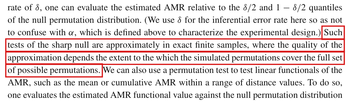
p. 144: “For a two-way test of the sharp null hypothesis for a specific AMR value with an error rate of δ\delta, one can evaluate the estimated AMR relative to the δ/2\delta/2 and 1−δ/21-\delta/2 quantiles of the null permutation distribution. … Such tests of the sharp null are approximately in exact finite samples, where the quality of the approximation depends the extent to the which the simulated permutations cover the full set of possible permutations.”

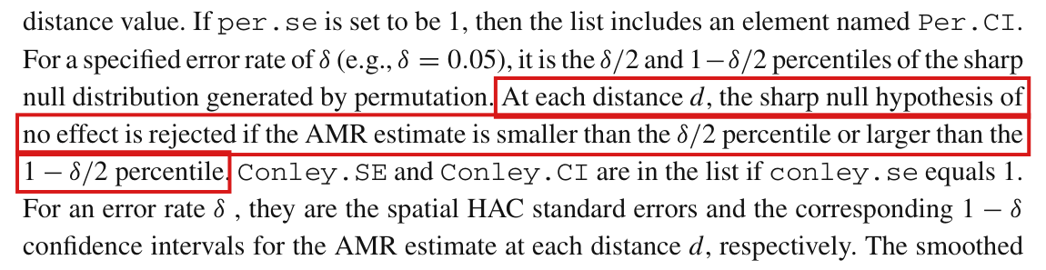
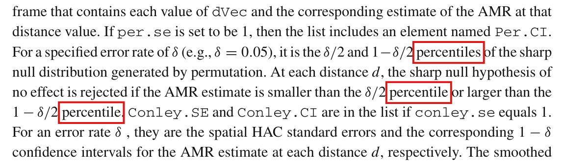
p. 146: “At each distance dd, the sharp null hypothesis of no effect is rejected if the AMR estimate is smaller than the δ/2\colorbox{#ffe58a}{$\delta/2$} percentile or larger than the 1−δ/2\colorbox{#ffe58a}{$1-\delta/2$} percentile.”

p. 148, footnote 5: “The number doesn’t make any difference here as there are in total 6 assignments.”

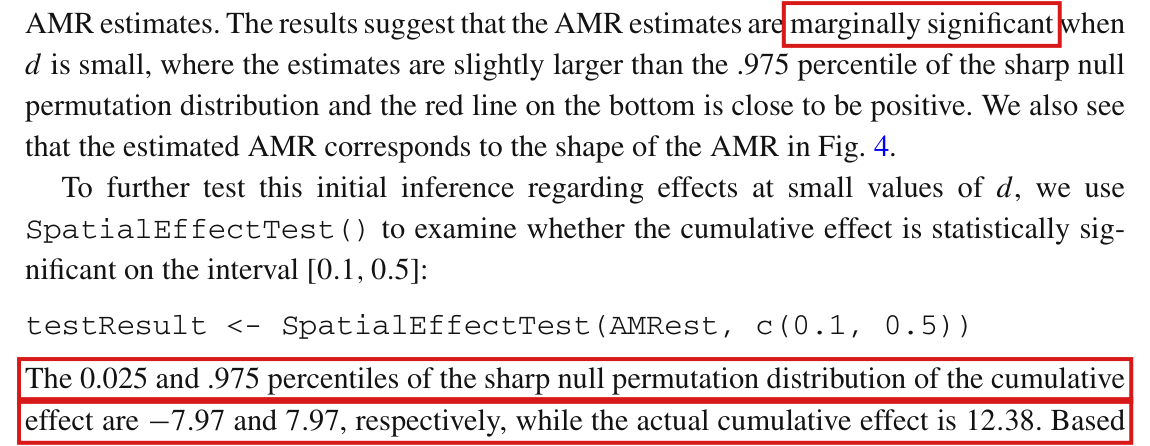
p. 149: “The results suggest that the AMR estimates are marginally significant when dd is small, where the estimates are slightly larger than the .975 percentile of the sharp null permutation distribution and the red line on the bottom is close to be positive.”

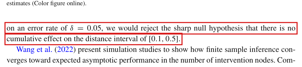
pp. 149–150: “The 0.025 and .975 percentiles of the sharp null permutation distribution of the cumulative effect are −7.97-7.97 and 7.977.97, respectively, while the actual cumulative effect is 12.38. Based [p. 150] on an error rate of δ=0.05\delta = 0.05, we would reject the sharp null hypothesis that there is no cumulative effect on the distance interval of [0.1,0.5][0.1, 0.5].”

The problem

The toy example has four nodes, two of them treated. The permutation distribution of footnote 5 consists of six assignments that are equally likely. It is the Bernoulli design of Section 4, conditional on two treated nodes. On such a set no nonrandomized test can reject at δ=0.05\delta=0.05, since a rejection region that contains a single assignment already has probability 1/61/6. For a difference in means with two nodes in each group more is true. The complementary assignment reverses the sign of the statistic, so at least two of the six values are as extreme as the observed one, and the exact two-sided p-value is at least 2/62/6.

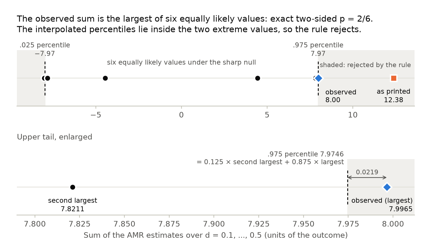
The printed rejection arises because the percentiles are interpolated. For six values, the default R quantile at level 0.9750.975 equals 0.1250.125 times the second largest value plus 0.8750.875 times the largest, which is below the largest value whenever the two differ. The rule of p. 146 rejects when the estimate is larger than this percentile or smaller than its counterpart at level 0.0250.025. It therefore rejects whenever the observed assignment gives the largest or the smallest of six distinct values. Under the sharp null this event has probability 2/62/6, not 0.050.05, and enumerating every permutation does not change it. The sentence on p. 144 attributes the error of the test to the number of simulated permutations; for this rule the error remains when all permutations are used.

In the toy example the observed cumulative statistic on [0.1,0.5][0.1,0.5] is 8.008.00 (the printed 12.3812.38 is corrected in P008-E003). It is the largest of the six values and exceeds the interpolated upper percentile by about 0.020.02. Its exact two-sided p-value is 2/6≈0.332/6\approx0.33, and the sharp null is not rejected at δ=0.05\delta=0.05. The sharp null is likewise not rejected at single distances. The estimates at d=0.4,…,0.7d=0.4,\dots,0.7 lie above the blue curve of Figure 5, and each has exact two-sided p-value 2/62/6; the estimates at d=0.1,0.2,0.3d=0.1,0.2,0.3 lie below it. As a statement about the randomization test, the words “marginally significant” are not supported at the 5% level at any distance.

Evidence an exact counterexample

The evidence is an exact counterexample to the rule, a derivation of the bound on the p-value, and a recalculation of the toy example.

Counterexample. Let four nodes have circle averages (0,1,2,3)(0,1,2,3) at each distance d=0.1,…,0.5d=0.1,\dots,0.5 and under every assignment, and let two of them be treated. Such outcomes are realized by a spatial field in which successive nodes on a line are 10 units apart and the outcome equals i−1i-1 within distance 1 of node ii and 00 elsewhere, whatever the assignment. This field satisfies the sharp null. For the six assignments, I find the following.

Sharp null true, circle averages (0,1,2,3)(0,1,2,3): the difference in means TT, its exact two-sided p-value, and the decision of the rule of p. 146 with interpolated percentiles.
AssignmentTTExact two-sided p-valueRule rejects
1100−2-21/31/3yes
1010−1-12/32/3no
10010011no
01100011no
0101112/32/3no
0011221/31/3yes

The interpolated percentiles at levels 0.0250.025 and 0.9750.975 are −15/8-15/8 and 15/815/8. The rule rejects for two of the six assignments, and its probability of rejection under the sharp null is 1/31/3. For the sum over the five distances 0.1,…,0.50.1,\dots,0.5 every value is multiplied by five, the percentiles are −75/8-75/8 and 75/875/8, and the same two assignments are rejected.

Bound on the p-value. Under the sharp null the circle averages mim_i do not depend on the assignment. For an assignment zz with two treated nodes, the estimator at one distance is

T(z)=12∑i=14zimi−12∑i=14(1−zi)mi=12∑i=14(2zi−1)mi,T(z)=\frac12\sum_{i=1}^{4}z_im_i-\frac12\sum_{i=1}^{4}(1-z_i)m_i=\frac12\sum_{i=1}^{4}(2z_i-1)m_i ,

and for the complementary assignment I have T(1−z)=−T(z)T(1-z)=-T(z). The same identity holds for a statistic SS that is a linear combination of the estimators at several distances. The exact two-sided p-value #{w:∣S(w)∣≥∣S(z)∣}/6\#\{w:\lvert S(w)\rvert\ge\lvert S(z)\rvert\}/6 counts both zz and 1−z1-z, so it is at least 2/62/6.

Recalculation. I generated the toy data as in the package vignette (seed 123567); the observed assignment treats nodes 1 and 2. The data reproduce the thirty printed entries of the columns AMR_est, Per.CI.l and Per.CI.u. The six values of the cumulative statistic on [0.1,0.5][0.1,0.5] are ±7.99649\pm7.99649, ±7.82109\pm7.82109 and ±4.44342\pm4.44342, and the observed value is 7.996497.99649. The interpolated percentiles are ±7.97457\pm7.97457, in agreement with the printed −7.97-7.97 and 7.977.97, and two of the six values are at least as extreme as the observed one. With the outcomes held fixed at the untreated raster, the rule rejects for two of the six assignments at each of the twenty distances. Both copies of the code in the archived repository of the package compute the percentiles with the R function quantile at its default setting. I did not have access to the release cited in the paper.
What survives

The definitions of the spatial potential outcomes and of the AMR, the toy point estimates and the curves of Figure 5 are unaffected. The cumulative statistic can still be used in a randomization test with a calibrated rule. The spatial-HAC intervals and the asymptotic claims are separate and are not addressed here. I find no additional error in the phrase “when dd is small”: it can refer to d=0.4,…,0.7d=0.4,\dots,0.7, where the estimates do exceed the upper percentile. The hypothesis tested is the sharp null, which Section 2.3 distinguishes from the weak null.

The toy rejection is withdrawn, and the rule of p. 146 and the sentence on p. 144 are replaced. What is shown is a failure of calibration for a design with six possible assignments. The application of Section 6 uses the same rule, and its p-value has to be recomputed on its own assignment distribution; whether its conclusion changes is not established here.

Corrected

p. 146, the rule. Let Ω\Omega be the set of assignments used for the permutation distribution, each with the same probability under the design (in the toy example, the six assignments with two treated nodes), and let S(z)S(z) be the statistic computed from the observed outcomes with assignment zz (the AMR estimate at one distance, or a linear functional such as the cumulative sum). Define the exact two-sided p-value

p=#{z∈Ω: ∣S(z)∣≥∣S(zobs)∣}∣Ω∣,p=\frac{\#\{z\in\Omega:\ \lvert S(z)\rvert\ge\lvert S(z_{\mathrm{obs}})\rvert\}}{\lvert\Omega\rvert},

which counts the observed assignment and all ties. “At each distance dd, the sharp null hypothesis of no effect is rejected if the exact two-sided p-value of the AMR estimate is at most δ\colorbox{#ffe58a}{$\delta$}.” Under the sharp null the probability of rejection is then at most δ\delta. Indeed, the outcomes are fixed under the sharp null, and the assignments with p≤δp\le\delta are contained in the set of assignments at least as extreme as the least extreme of them, which has at most δ∣Ω∣\delta\lvert\Omega\rvert elements. Critical values calibrated conservatively for the discrete distribution are an alternative to the p-value. If the assignments have unequal probabilities, the entire fraction is replaced by the sum of the probabilities of the assignments counted. If Ω\Omega is too large to enumerate and BB assignments Z1,…,ZBZ_1,\dots,Z_B are drawn independently from the design, independently of the observed assignment, the Monte Carlo p-value is

p=1+#{b: ∣S(Zb)∣≥∣S(zobs)∣}B+1.p=\frac{1+\#\{b:\ \lvert S(Z_b)\rvert\ge\lvert S(z_{\mathrm{obs}})\rvert\}}{B+1}.

p. 144: “Such tests of the sharp null have level δ\delta in finite samples when the decision is based on the exact two-sided p-value. Interpolated δ/2\delta/2 and 1−δ/21-\delta/2 quantiles need not give a test of level δ\delta, even when every permutation is enumerated.”

p. 149: “The AMR estimates at d=0.4,…,0.7d=0.4,\dots,0.7 are slightly larger than the interpolated .975 percentile of the sharp null permutation distribution; each has exact two-sided p-value 2/62/6.”

pp. 149–150: “The 0.025 and .975 percentiles of the sharp null permutation distribution of the cumulative effect are −7.97-7.97 and 7.977.97, respectively, while the actual cumulative effect is 8.00, the largest of the six possible values. Its exact two-sided p-value is 2/6≈0.332/6\approx0.33, so the sharp null hypothesis is not rejected at δ=0.05\delta=0.05. With six equally likely assignments, no nonrandomized test can reject at this level.”

Crop of the last line of the Figure 5 caption and four lines of text. Red boxes mark the two lines 'on an error rate of delta = 0.05, we would reject the sharp null hypothesis that there is no cumulative effect on the distance interval of [0.1, 0.5].'
Section 5, p. 150 (PDF p. 13), first sentence of text below Figure 5. The marked sentence, which begins on p. 149, rejects the sharp null at δ=0.05\delta=0.05.
Crop of nine lines of text and one line of code. Red boxes mark the words 'marginally significant' in the sentence 'The results suggest that the AMR estimates are marginally significant when d is small', and the last two lines, 'The 0.025 and .975 percentiles of the sharp null permutation distribution of the cumulative effect are minus 7.97 and 7.97, respectively, while the actual cumulative effect is 12.38. Based'.
Section 5, p. 149 (PDF p. 12), text after the output table. The marked words call the estimates marginally significant, and the marked lines compare the cumulative statistic with the two percentiles.
Crop of seven lines of text. Red boxes mark the sentence 'At each distance d, the sharp null hypothesis of no effect is rejected if the AMR estimate is smaller than the delta over 2 percentile or larger than the 1 minus delta over 2 percentile.', which runs over three lines.
Section 3, p. 146 (PDF p. 9). The marked sentence is the rejection rule: reject when the estimate lies outside the two percentiles.
Crop of eight lines of text. Red boxes mark the sentence 'Such tests of the sharp null are approximately in exact finite samples, where the quality of the approximation depends the extent to the which the simulated permutations cover the full set of possible permutations.', which runs over four lines.
Section 2.3, p. 144 (PDF p. 7). The marked sentence attributes the error of the test to the number of simulated permutations.
Crop of one footnote line, 'The number doesn't make any difference here as there are in total 6 assignments.' A red box marks the words 'in total 6 assignments'.
Footnote 5, p. 148 (PDF p. 11). The marked words give the number of assignments in the permutation distribution of the toy example.
Two horizontal strips under the title 'The observed sum is the largest of six equally likely values: exact two-sided p = 2/6. The interpolated percentiles lie inside the two extreme values, so the rule rejects.' The upper strip runs from minus 9.6 to 13.6 and shows six points at about minus 8.00, minus 7.82, minus 4.44, 4.44, 7.82 and 8.00; dashed vertical lines at minus 7.97 and 7.97 are labelled .025 percentile and .975 percentile, and the regions beyond them are shaded and labelled 'rejected by the rule'. A blue diamond labelled 'observed 8.00' sits just right of the upper dashed line, and an orange square labelled 'as printed 12.38' sits far to the right. The lower strip, titled 'Upper tail, enlarged', runs from 7.79 to 8.012 and shows a black point labelled 'second largest 7.8211', a dashed line labelled '.975 percentile 7.9746 = 0.125 times second largest + 0.875 times largest', and the blue diamond labelled 'observed (largest) 7.9965', with an arrow of length 0.0219 between the line and the diamond. The horizontal axis is the sum of the AMR estimates over d = 0.1 to 0.5, in units of the outcome.
The six possible values of the cumulative statistic on [0.1,0.5][0.1,0.5] in the toy example, with the interpolated percentiles (dashed), the observed value (blue diamond) and the value printed on p. 149 (orange square). The lower panel enlarges the upper tail. The observed value is the largest of the six and lies 0.02190.0219 above the upper percentile.

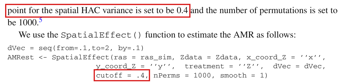
In the later archived version of the package, the bandwidth of the spatial-HAC variance of the unsmoothed estimator is cutoff plus the position of the radius in dVec, and not the distance threshold that the paper describes; the bandwidth should be cutoff itself, or a stated function of the radius in the units of the distances.

Section 3, p. 145 (PDF p. 8), sentence on cutoff; file R/SpatialEffect.R of the later archived version of the package, lines 199–219 (the code is not printed in the article)

See also under Formal statements (Lean): P008-T9, P008-T10

As printed

p. 145. For the asymptotic variance estimator, users need to specify a distance threshold (cutoff) beyond which interference dependence does not exist.

Later archived version of the package, R/SpatialEffect.R, lines 199–201 and 215–219.

c <- cutoff

for (d in 1:length(dVec)){

dUp <- dVec[d]

…

if (cutoff > 0){

c <- cutoff + d

}

Conley_result <- ConleySE(as.vector(res_d), as.matrix(W_meat), as.matrix(dist),

as.double(c), as.integer(k))

The problem

The paper describes cutoff as a distance: pairs of nodes farther apart than cutoff contribute no covariance terms to the variance estimate. The later version of the package is the one distributed with the replication files of Wang, Samii, Chang and Aronow (2024). In its loop over the radii, the spatial-HAC standard error of the unsmoothed estimator is computed with the bandwidth cutoff + d whenever cutoff is positive. Here d is the index 1,2,3,…1,2,3,\ldots of the loop, and the radius itself is dUp. The bandwidth for a radius therefore depends on the place of that radius in the grid of radii dVec, rather than on the radius itself.

Two consequences follow. The standard error of the estimate at a given radius can change when another radius is inserted before it in dVec, although the estimate and the data are the same. Further, the bandwidth grows by one unit of the distance matrix with each entry of the grid, whatever the unit is. In the units of the toy example it exceeds every distance between two nodes at the sixth radius, 0.60.6, and the variance there is exactly zero under the default uniform kernel and edf = FALSE. When spatial-HAC intervals are requested with a positive cutoff, the function passes this index-based bandwidth without warning.

Evidence an exact counterexample

I checked an exact counterexample in rational arithmetic and the output printed on p. 149. The unchanged R function in the later version, supplied with the counterexample’s circle averages and distances and an R implementation of the uniform-kernel variance formula, returns the same bandwidths and variances.

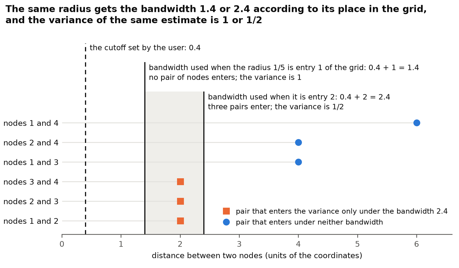
Counterexample. Let four nodes lie at (0,0)(0,0), (2,0)(2,0), (4,0)(4,0) and (6,0)(6,0), with treatments Z=(0,0,1,1)Z=(0,0,1,1), and let the outcome equal 00, 22, 44 and 66 on the discs of radius 3/103/10 around them. The circle averages are μ=(0,2,4,6)\mu=(0,2,4,6) at each of the radii 1/101/10, 1/51/5 and 3/103/10. I take Euclidean distance, the uniform kernel, edf = FALSE and cutoff =2/5=2/5. The regression of μ\mu on an intercept and ZZ has coefficients (1,4)(1,4) and residuals r=(−1,1,−1,1)r=(-1,1,-1,1), and the estimate is 44. The weights of the treatment coefficient are a=(−1/2,−1/2,1/2,1/2)a=(-1/2,-1/2,1/2,1/2). With the scores gi=airig_i=a_ir_i, that is, g=(1/2,−1/2,−1/2,1/2)g=(1/2,-1/2,-1/2,1/2), the variance with bandwidth cc is

V(c)=∑i,jgigj 1{Dij≤c},V(c)=\sum_{i,j}g_ig_j\,\mathbf{1}\{D_{ij}\le c\},

where DijD_{ij} is the distance between nodes ii and jj. If c<2c<2, only the terms with i=ji=j remain, and V(c)=∑igi2=1V(c)=\sum_i g_i^2=1. If 2≤c<42\le c<4, the three pairs of neighbors enter as well, and V(c)=1+2(g1g2+g2g3+g3g4)=1+2(−1/4+1/4−1/4)=1/2V(c)=1+2(g_1g_2+g_2g_3+g_3g_4)=1+2(-1/4+1/4-1/4)=1/2.

The same radius 1/51/5 on two grids of radii, under the rule of the later version and under a bandwidth equal to cutoff.
Grid of radiiPlace of 1/51/5BandwidthEstimateVarianceStandard error
(1/5, 3/10)(1/5,\ 3/10)12/5+1=7/52/5+1=7/5441111
(1/10, 1/5, 3/10)(1/10,\ 1/5,\ 3/10)22/5+2=12/52/5+2=12/5441/21/20.70710.7071
Either grid, bandwidth cutoff1 or 22/52/5441111

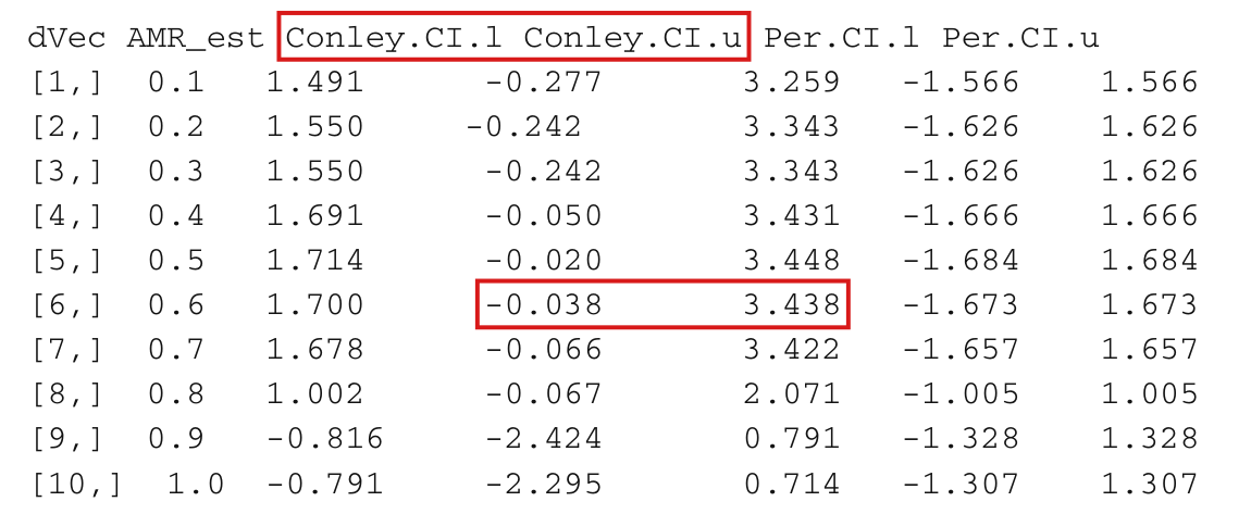
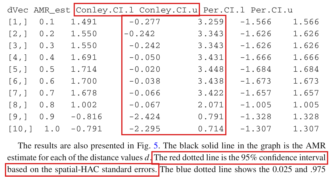
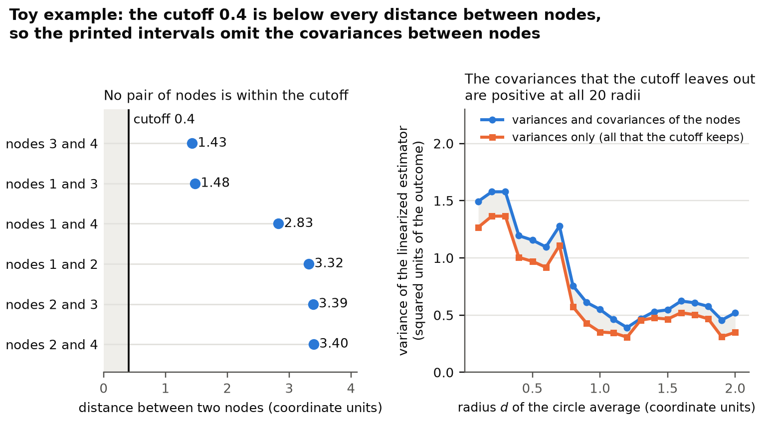
The printed output. Since the four nodes of the toy example lie in the square [0,4]2[0,4]^2 (Figure 2), two of them are at most 32\sqrt{32} apart. The printed call has cutoff = .4 and radii 0.1,0.2,…,20.1,0.2,\ldots,2, and it leaves the kernel at its default, the uniform kernel. At the sixth radius the rule of the later version gives the bandwidth 0.4+6=6.4>320.4+6=6.4>\sqrt{32}, and the kernel includes every pair of nodes. Then the variance is (∑igi)2(\sum_i g_i)^2, which is zero for any data, since the residuals of a regression on an intercept and the treatment sum to zero in each arm. The interval at d=0.6d=0.6 would have width zero. The printed interval is [−0.038, 3.438][-0.038,\,3.438], of width 3.4763.476, and I conclude that this rule did not produce the printed table.

What survives

The sentence on p. 145 is correct as a description of the method. The definition of the AMR, the unsmoothed point estimates and permutation tests do not use this line, and the line is skipped when cutoff = 0. I attribute no published interval to the defect: the release that the paper cites is not archived, the earlier archived version of the package passes cutoff unchanged, and the printed toy intervals are incompatible with the rule. The later version’s requested spatial-HAC standard errors and intervals of the unsmoothed estimator depend on this bandwidth. With edf = TRUE, so do those of the smoothed estimator and its confidence bands, which reuse the degrees of freedom computed in the same loop.
Corrected

The sentence on p. 145 needs no change. If cutoff is the final node-pair dependence threshold, I delete lines 215–217 in the later version of the package, so that the bandwidth passed to the variance routine is that threshold:

c <- cutoff

for (d in 1:length(dVec)){

dUp <- dVec[d]

…

if (cutoff > 0){ c <- cutoff + d }

Conley_result <- ConleySE(as.vector(res_d), as.matrix(W_meat), as.matrix(dist),

as.double(c), as.integer(k))

With this change the variance in the counterexample is 11 on both grids. If cutoff is instead meant as a range of interference that has to be enlarged for circle averages of radius dd, then the bandwidth must be a stated function of the radius dUp, in the units of the distance matrix, and never of the index d. Which enlargement is right is not established here. Replacing d by dUp removes the dependence on the grid, but it does not by itself establish that the resulting intervals are valid.

Crop of five lines of text. The marked sentence reads: For the asymptotic variance estimator, users need to specify a distance threshold (cutoff) beyond which interference dependence does not exist. It is followed by: This can be based on substantive judgments about the likely spatial extent of interference, and can be varied as part of a sensitivity analysis. Red outlines surround the words distance threshold (cutoff) beyond which interference dependence does not exist.
Section 3, p. 145 (PDF p. 8). The outlines mark the description of cutoff as a distance threshold.
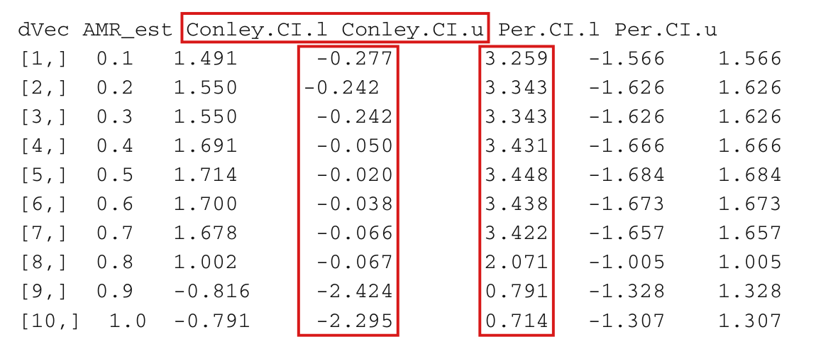
Crop of a printed table with ten rows and the columns dVec, AMR\_est, Conley.CI.l, Conley.CI.u, Per.CI.l and Per.CI.u. Row 6 reads: 0.6, 1.700, -0.038, 3.438, -1.673, 1.673. Red outlines surround the column headings Conley.CI.l and Conley.CI.u and the two values -0.038 and 3.438 in row 6.
Output of summary(), p. 149 (PDF p. 12). The outlines mark the two columns of the spatial-HAC interval and the row for d=0.6d=0.6, where the rule of the later version would give an interval of width zero.
Dot plot with the distance between two nodes on the horizontal axis, from 0 to 6.6 units of the coordinates, and one row for each of the six pairs of nodes. Three orange squares at distance 2 are the pairs of nodes 1 and 2, 2 and 3, and 3 and 4. Two blue circles at distance 4 are the pairs 1 and 3, and 2 and 4. One blue circle at distance 6 is the pair 1 and 4. A dashed vertical line at 0.4 is labelled the cutoff set by the user. A solid vertical line at 1.4 is labelled bandwidth used when the radius 1/5 is entry 1 of the grid: 0.4 + 1 = 1.4, no pair of nodes enters, the variance is 1. A solid vertical line at 2.4 is labelled bandwidth used when it is entry 2: 0.4 + 2 = 2.4, three pairs enter, the variance is 1/2. The region between 1.4 and 2.4 is shaded and contains the three orange squares. The legend says that orange squares are pairs that enter the variance only under the bandwidth 2.4 and blue circles are pairs that enter under neither bandwidth.
The counterexample. The six pairs of nodes are 2, 4 or 6 units apart. When the radius 1/51/5 is the first entry of the grid, the later version uses the bandwidth 1.41.4, no pair enters and the variance is 11. When it is the second entry, the bandwidth is 2.42.4, the three pairs of neighbors enter and the variance is 1/21/2. The cutoff set by the user is 0.40.4 in both cases.

The printed −0.0321-0.0321, −0.0304-0.0304 and 0.03360.0336 are unweighted sums of AMR estimates at several distances, not changes of 3.21, 3.04 and 3.36 percentage points in a probability of forest loss.

Section 6, paragraph after the SpatialEffectTest() call, p. 153 (PDF p. 16), both parentheticals

See also under Formal statements (Lean): P008-T7, P008-T8, P008-T24

As printed

For the cumulative effect between 1 km and 2.5 km, the 0.025 and .975 percentiles of the sharp null permutation distribution are −0.0304-0.0304 and 0.03360.0336 (that is, a 3.04 percentage point reduction to a 3.36 percentage point increase in the cumulative probability of forest loss), respectively. The estimated cumulative effect between 1 km and 2.5 km is −0.0321-0.0321 (i.e., a 3.21 percentage point reduction).
The problem

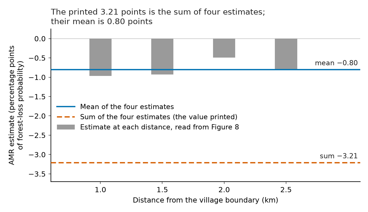
The cumulative statistic is the sum of the AMR estimates at the distances in the window, each with weight one (the summation is described on p. 146). Each AMR τ(d)\tau(d) is a difference of two circle-average probabilities of forest loss at distance dd, averaged over villages and over the other villages' assignments, with the selected village treated and not treated. A sum of mm such differences need not be a difference of probabilities. For a probability defined by mixing these circle averages over distances, the change is a weighted average ∑jwjτ(dj)\sum_j w_j \tau(d_j) with nonnegative weights that sum to one. The weights of the printed statistic sum to mm. The two parentheticals read the sum and its null percentiles as percentage-point changes in “the cumulative probability of forest loss”, and the unit weights of the sum do not define such a probability. Figure 8 shows four estimates in the window, at 1, 1.5, 2 and 2.5 km. For this four-distance grid, dividing the printed sum −0.0321-0.0321 by four gives a mean estimate of about −0.0080-0.0080, an estimated reduction of 0.8 percentage points. The value 3.21 is the only effect size quoted for the application.


The printed values, and the same values as an equally weighted mean over four distances.
QuantityAs printed (sum)Divided by four (mean)
0.025 percentile of the null distribution−0.0304-0.0304−0.0076-0.0076
Observed statistic−0.0321-0.0321−0.008025-0.008025
0.975 percentile of the null distribution0.03360.03360.00840.0084
Evidence an exact counterexample

My evidence is a derivation and an exact counterexample: for loss probabilities QbQ_b defined by drawing a village uniformly, setting its assignment to bb, drawing a distance with probabilities wjw_j, and using the paper’s circle-average measure, with other assignments averaged over the design, I obtain

Q1−Q0=∑j=1mwjτ(dj),wj≥0,∑j=1mwj=1.Q_1 - Q_0 = \sum_{j=1}^m w_j \tau(d_j), \qquad w_j \ge 0, \quad \sum_{j=1}^m w_j = 1.

For the counterexample, I take four village centres at least 20 km apart and 40000 points on each circle at distances 1, 1.5, 2 and 2.5 km, with independent assignments of probability 1/21/2 and binary outcomes defined on all 640000 circle points and all four centres for every assignment. At the assignment (1,1,0,0)(1,1,0,0), each AMR and its Hajek estimate equal −0.008025-0.008025, giving sum −0.0321-0.0321, while the constructed pooled loss probabilities are 0.01750.0175 under control and 0.0094750.009475 under treatment, a change of −0.8025-0.8025 percentage points. Reading the sum as this probability change would give 0.0175−0.0321=−0.0146<00.0175 - 0.0321 = -0.0146 < 0 under treatment; a companion binary model on the same spatial field gives sum −4-4 and probability change −1-1, ruling out a general conversion of the sum into a probability change.

What survives

The AMR, the Hajek estimator and the use of a fixed sum of AMR estimates as the statistic of a sharp-null test are unaffected by this interpretation error. Dividing the statistic and every permutation value by the same positive number preserves ranks and the printed comparison −0.0321<−0.0304-0.0321 < -0.0304, provided that the statistic and the percentiles use the same grid; the original application percentiles and exact pp-value have not been independently reproduced. The summed AMR statistic does not represent a 3.21-percentage-point reduction in a probability of forest loss; the grid in the printed code has no distance inside the window, which is the subject of P008-E004.

Corrected

For the sum of the AMR estimates at the distances evaluated between 1 km and 2.5 km, each with weight one, the 0.025 and .975 percentiles of the sharp null permutation distribution are −0.0304-0.0304 and 0.03360.0336, respectively. The observed sum is −0.0321-0.0321, which lies below the lower percentile. These numbers are values of a summed AMR statistic and are not changes in a probability of forest loss.

If the grid consists of the four distances 1, 1.5, 2 and 2.5 km shown in Figure 8, the equally weighted mean of the four estimates, using the printed sum, is −0.0321/4=−0.008025-0.0321/4 = -0.008025. This estimates a reduction of about 0.8 percentage points for a probability of forest loss that gives equal weight to each distance and each village and uses the paper’s circle averages. On the same scale the percentiles are −0.0304/4=−0.0076-0.0304/4 = -0.0076 and 0.0336/4=0.00840.0336/4 = 0.0084. The text should state the grid of distances that was used.

Six lines of text from page 153. Red boxes mark two parentheticals. The first reads: that is, a 3.04 percentage point reduction to a 3.36 percentage point increase in the cumulative probability of forest loss. The second reads: i.e., a 3.21 percentage point reduction.
Section 6, paragraph after the test call, p. 153 (PDF p. 16). The two marked parentheticals read the summed statistic and its null percentiles as percentage-point changes in a probability of forest loss.
Bar chart of four AMR estimates at 1, 1.5, 2 and 2.5 km, in percentage points: about -0.97, -0.93, -0.49 and -0.82. A solid blue horizontal line marks their mean at -0.80. A dashed orange horizontal line marks their sum multiplied by 100 at -3.21, far below every bar; this sum is not a probability change.
The four estimates in the window from 1 to 2.5 km, read from the black curve in the top-left panel of Figure 8 (p. 154; PDF p. 17), with their mean and their sum, each multiplied by 100. The sum is about −3.21-3.21 on this scale and is not a probability change; the mean is about −0.80-0.80 percentage points.

Minor (17)

Real but inconsequential, for example a misprint that does not change a result.

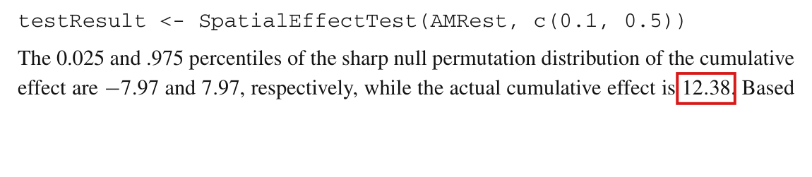
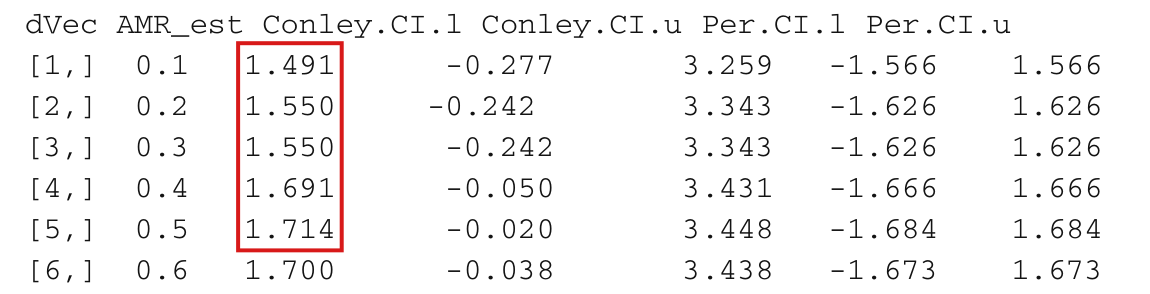
The observed cumulative statistic on [0.1,0.5][0.1,0.5] is 8.008.00, the sum of the five printed AMR estimates; the printed 12.3812.38 matches the sum of the estimates through d=0.8d=0.8.

Section 5, last sentence of p. 149 (PDF p. 12), after the call to SpatialEffectTest(); output table on the same page

See also under Formal statements (Lean): P008-T11

As printed

testResult <- SpatialEffectTest(AMRest, c(0.1, 0.5))

“The 0.025 and .975 percentiles of the sharp null permutation distribution of the cumulative effect are −7.97-7.97 and 7.977.97, respectively, while the actual cumulative effect is 12.38.”

Output table on the same page, columns dVec and AMR_est.
dVec0.10.10.20.20.30.30.40.40.50.50.60.60.70.70.80.80.90.91.01.0
AMR_est1.4911.4911.5501.5501.5501.5501.6911.6911.7141.7141.7001.7001.6781.6781.0021.002−0.816-0.816−0.791-0.791
The problem

Section 3 (p. 146) says that SpatialEffectTest() “generates the null permutation distribution of the sum of the AMR estimates within the specified range”. The “actual cumulative effect” for the range [0.1,0.5][0.1,0.5] is therefore the sum of the estimates at d=0.1,…,0.5d=0.1,\dots,0.5. The five printed estimates sum to 7.9967.996, not to 12.3812.38. Note that the percentiles −7.97-7.97 and 7.977.97 do belong to [0.1,0.5][0.1,0.5]. The sentence compares the percentiles of one range with a number that matches the observed sum on a wider range. It suggests a margin of about 4.44.4 above the upper percentile, and the margin is 0.020.02.

Evidence a historical Lean attribution (Generated status: clause support not certified in this release)

The evidence is a derivation from the printed table and a recalculation of the toy example. From the printed estimates, I have

1.491+1.550+1.550+1.691+1.714=7.996.1.491+1.550+1.550+1.691+1.714=7.996 .

Each printed estimate is within 0.00050.0005 of its unrounded value, so the unrounded sum lies in [7.9935, 7.9985][7.9935,\,7.9985]. A number printed as 12.3812.38 lies in [12.375, 12.385][12.375,\,12.385], and the two intervals are disjoint. Adding the next three estimates, I obtain 7.996+1.700+1.678+1.002=12.3767.996+1.700+1.678+1.002=12.376, which rounds to 12.3812.38. A sum multiplied by the step 0.10.1 of the grid would be 0.79960.7996.

For the recalculation, I generated the toy data as in the package vignette (seed 123567) and enumerated the six assignments with two treated nodes. These data reproduce the ten printed estimates and their permutation bounds, and give the following.

The cumulative statistic and its interpolated percentiles on two ranges, recalculated.
RangeObserved sum.025 and .975 percentiles
[0.1, 0.5][0.1,\,0.5]7.996497.99649−7.97457-7.97457, 7.974577.97457
[0.1, 0.8][0.1,\,0.8]12.3757112.37571−12.30669-12.30669, 12.3066912.30669

The SpatialEffectTest() function in the archived repository of the package returns the same values. The release of the package cited in the paper and the script that produced the number are not available. The agreement with the sum through d=0.8d=0.8 is a numerical fact and does not show how 12.3812.38 arose.

What survives

The ten AMR estimates, their permutation bounds and the percentiles −7.97-7.97 and 7.977.97 stand, and no later result is computed from this number. The corrected sum still exceeds the upper percentile, by 0.0220.022. The conclusion drawn from that comparison on p. 150, a rejection at δ=0.05\delta=0.05, fails for a separate reason given in P008-E002.

Corrected

“The 0.025 and .975 percentiles of the sharp null permutation distribution of the cumulative effect are −7.97-7.97 and 7.977.97, respectively, while the actual cumulative effect is 8.00.”

The unrounded sum is 7.996497.99649. It exceeds the upper interpolated percentile, 7.974577.97457, by 0.021930.02193. With six equally likely assignments the exact two-sided p-value of this sum is 1/31/3, so the example does not establish a rejection of the sharp null at the 5% level.

Crop of three lines: the code line 'testResult <- SpatialEffectTest(AMRest, c(0.1, 0.5))' and the sentence 'The 0.025 and .975 percentiles of the sharp null permutation distribution of the cumulative effect are minus 7.97 and 7.97, respectively, while the actual cumulative effect is 12.38.' A red box marks the number 12.38.
Section 5, last lines of p. 149 (PDF p. 12). The marked number is reported as the cumulative statistic for the call above it, whose range is [0.1,0.5][0.1,0.5].
Crop of the header and first six rows of the printed output table, with columns dVec, AMR_est, Conley.CI.l, Conley.CI.u, Per.CI.l and Per.CI.u. A red box marks the AMR_est entries of rows 1 to 5: 1.491, 1.550, 1.550, 1.691 and 1.714.
Output table, p. 149 (PDF p. 12), first six rows. The five marked AMR estimates, at d=0.1,…,0.5d=0.1,\dots,0.5, sum to 7.9967.996.

The step of the distance grid is 0.5/111≈0.00450.5/111\approx0.0045, that is, 0.5 km, and not 5/111≈0.0455/111\approx0.045; with the printed step no grid point lies in the test range of 1 to 2.5 km.

Section 6, first paragraph and the two printed calls, p. 153 (PDF p. 16); Figure 8, p. 154 (PDF p. 17)

See also under Formal statements (Lean): P008-T12, P008-T13

As printed

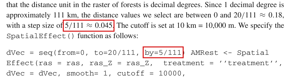
“Since 1 decimal degree is approximately 111 km, the distance values we select are between 0 and 20/111≈0.1820/111 \approx 0.18, with a step size of 5/111≈0.045\colorbox{#ffe58a}{$5/111 \approx 0.045$}.”

dVec = seq(from=0, to=20/111, by=5/111) AMRest <- Spatial

Effect(ras = ras, ras_Z = ras_Z, treatment = ’’treatment’’,

dVec = dVec, smooth= 1, cutoff = 10000,

dist.metric = ’’Geodesic’’)

testResult <- SpatialEffectTest(AMRest, test.range = c(1/111,

2.5/111))

“The estimated cumulative effect between 1 km and 2.5 km is −0.0321-0.0321 (i.e., a 3.21 percentage point reduction).”

The problem

The printed grid seq(from=0, to=20/111, by=5/111) has five points, at 0, 5, 10, 15 and 20 km. The test range is [1/111, 2.5/111][1/111,\,2.5/111], that is, 1 to 2.5 km, and none of the five points lies in it. By Section 3 (p. 146), SpatialEffectTest() sums the AMR estimates at the grid points within the range. With the printed grid the observed sum and every permuted sum are empty sums, equal to zero, and the reported statistic −0.0321-0.0321 and percentiles −0.0304-0.0304 and 0.03360.0336 cannot come from the printed commands.

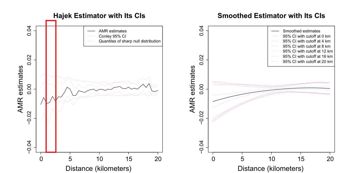
Figure 8 shows the grid that was used. Its unsmoothed curve has 41 points at a spacing of 0.5 km, and the four estimates at 1, 1.5, 2 and 2.5 km sum to −0.0321-0.0321. The step 5/1115/111 is a misprint for 0.5/1110.5/111, in the text and in the code.

Evidence an exact counterexample

The evidence is a derivation and a check of Figure 8. The printed grid is dk=5k/111d_k=5k/111 for k=0,…,4k=0,\dots,4. The condition dk∈[1/111, 2.5/111]d_k\in[1/111,\,2.5/111] is equivalent to 1≤5k≤5/21\le 5k\le 5/2, which fails for k=0k=0 and for every k≥1k\ge 1. The SpatialEffectTest() function in the archived repository of the package, run with the printed grid on an example with four nodes and all six assignments enumerated, returns an observed sum of 00 and both percentiles equal to 00.

In the PDF, the black line of the Hajek panel of Figure 8 is a polyline with 41 vertices. Their horizontal positions agree with 0,0.5,…,200,0.5,\dots,20 km to within 0.00020.0002 km. The values at the four vertices in the test range, read from the axes of the figure, are as follows.

The four plotted AMR estimates of Figure 8 in the range of 1 to 2.5 km.
Distance (km)AMR estimate read from the plot
1.01.0−0.00968-0.00968
1.51.5−0.00927-0.00927
2.02.0−0.00493-0.00493
2.52.5−0.00821-0.00821
Sum−0.03209-0.03209

The sum rounds to the reported −0.0321-0.0321. These values are read from a published graphic and are not a recalculation from the data of the application, which are not available.

What survives

No reported number or conclusion changes: Figure 8 and the reported cumulative statistic agree with a grid of step 0.5 km. The correction concerns the grid only. The percentiles −0.0304-0.0304 and 0.03360.0336 and the statement p<0.05p<0.05 could not be recomputed and are not certified by it. The units of the cumulative statistic are the subject of P008-N016, and the layout of the printed call that of P008-E009.

Corrected

“Since 1 decimal degree is approximately 111 km, the distance values we select are between 0 and 20/111≈0.1820/111 \approx 0.18, with a step size of 0.5/111≈0.0045\colorbox{#ffe58a}{$0.5/111 \approx 0.0045$}.”

dVec = seq(from=0, to=20/111, by=0.5/111)

The grid then has 41 points, at 0,0.5,…,200,0.5,\dots,20 km, and the four points at 1, 1.5, 2 and 2.5 km lie in the test range. The object AMRest has to be computed on this grid before the test is run. A full replication of the test also needs the transformed inputs of the application and the release of the package used for the paper, which are not available.

Crop of four lines of text and three lines of code. Red boxes mark '5/111 approximately equal to 0.045' in the sentence 'with a step size of 5/111 approximately 0.045', and 'by=5/111' in the code line 'dVec = seq(from=0, to=20/111, by=5/111) AMRest <- Spatial'.
Section 6, p. 153 (PDF p. 16). The marked step size in the text and the marked argument in the code both give a step of 5 km.
Crop of the two upper panels of Figure 8, 'Hajek Estimator with Its CIs' on the left and 'Smoothed Estimator with Its CIs' on the right, each with AMR estimates from minus 0.04 to 0.04 against distance from 0 to 20 kilometres. In the left panel a jagged black line with many short segments runs from about minus 0.01 at 0 km to about 0 at 20 km, between dotted red and blue lines. A tall red box marks the vertical band between 1 and 2.5 km in the left panel.
Figure 8, upper panels, p. 154 (PDF p. 17). The marked band is the test range of 1 to 2.5 km in the panel of the Hajek estimator. The black curve has a point every 0.5 km, and four of its points lie in the band.

The argument that sets the error rate δ\delta is alpha, not conley.se; the argument conley.se switches the spatial-HAC output on and off.

Section 3, p. 145 (PDF p. 8), last paragraph, second sentence

As printed

As discussed in the previous section, the package provides users with two inference methods, a Fisher-style permutation test (per.se) and an asymptotic variance estimator based on Conley (1999) (conley.se). Users can change the error rate δ\delta defining the level of statistical significance (conley.se).

The problem

Since the names in parentheses in Section 3 are arguments of SpatialEffect(), the sentence says that conley.se sets the level δ\delta. The next page says that Conley.SE and Conley.CI are returned “if conley.se equals 1”, and in both archived versions of the package the level is the argument alpha, with default 0.05. In those versions, setting conley.se = 0.05 skips the unsmoothed spatial-HAC output.

Evidence a check of the printed page

I checked the page against p. 146 and against the argument lists and manuals of both archived versions of the package. The condition conley.se == 1 in the source is false at the value 0.05, and the block that computes the unsmoothed spatial-HAC standard errors is then skipped. The release that the paper cites (version 0.1) is not archived, and I did not examine it.

What survives

Users can change the level, as the sentence says, and the first (conley.se) in the paragraph is correct. The two printed calls (pp. 148 and 153) set neither argument, and no reported number is affected.

Corrected

Users can change the error rate δ\delta defining the level of statistical significance (alpha).

Crop of five lines of text. The text reads: As discussed in the previous section, the package provides users with two inference methods, a Fisher-style permutation test (per.se) and an asymptotic variance estimator based on Conley (1999) (conley.se). Users can change the error rate delta defining the level of statistical significance (conley.se). The permutation test can be adjusted to account for blocking or clustering in experimental design. For the asymptotic variance estimator. A red outline surrounds the second (conley.se), the one after the words statistical significance.
Section 3, p. 145 (PDF p. 8), last paragraph. The outline marks the second (conley.se), which should read (alpha).

The circular band consists of outcome points, not of intervention nodes.

Section 2.2, p. 143 (PDF p. 6), paragraph after the circle-average display, sentence beginning “Another option that the SpatialEffect package offers”

See also under Formal statements (Lean): P008-T15

As printed

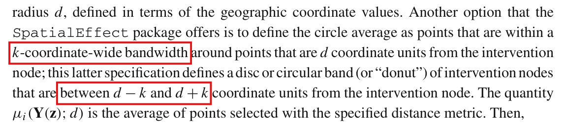
Another option that the SpatialEffect package offers is to define the circle average as points that are within a kk-coordinate-wide bandwidth around points that are dd coordinate units from the intervention node; this latter specification defines a disc or circular band (or “donut”) of intervention nodes that are between d−kd-k and d+kd+k coordinate units from the intervention node.

The problem

Since the band is the set over which outcomes are averaged, it consists of points xx at which outcomes are defined. Section 2.1 indexes these points separately from the intervention nodes ii, and the words “of intervention nodes” name the wrong set.

Evidence a check of the printed page

I checked the page against the definitions on p. 141 and the circle-average display on p. 143, which integrates Yx(z)Y_x(\mathbf{z}) over the points xx such that di(x)=dd_i(x)=d, for one intervention node ii.

What survives

The formulas and the computations use outcome points, and nothing depends on the phrase. The width of the band is the subject of P008-N001.

Corrected

… this latter specification defines a disc or circular band (or “donut”) of outcome points that are between d−kd-k and d+kd+k coordinate units from the intervention node.

Crop of five lines of text. The text reads: SpatialEffect package offers is to define the circle average as points that are within a k-coordinate-wide bandwidth around points that are d coordinate units from the intervention node; this latter specification defines a disc or circular band (or donut) of intervention nodes that are between d minus k and d plus k coordinate units from the intervention node. The quantity mu i of Y of z and d is the average of points selected with the specified distance metric. Then. A red outline surrounds the words of intervention nodes.
Section 2.2, p. 143 (PDF p. 6), paragraph after the circle-average display. The outline marks the phrase that names the wrong set.

Four sentences contain slips of copy: read “outcomes that are at a given distance” (p. 140), “approximately exact in finite samples” and “depends on the extent to which” (p. 144), “remunerate” (p. 150) and “which was the case” (p. 153).

Section 1, p. 140 (PDF p. 3); Section 2.3, p. 144 (PDF p. 7); Section 6, p. 150 (PDF p. 13) and p. 153 (PDF p. 16)

As printed

p. 140. The AMR measures how, on average, outcomes that at a given distance from an intervention site are affected by activating treatment at that site, taking into account ambient effects emanating from other intervention sites.

p. 144. Such tests of the sharp null are approximately in exact finite samples, where the quality of the approximation depends the extent to the which the simulated permutations cover the full set of possible permutations.

p. 150. PES programs are a form of environmental governance that financially renumerate landowners for environmental performance, …

p. 153. The key reason for why we find more compelling evidence is that our analysis is not restricted to forest loss within the village boundaries per se, which was that case for Jayachandran et al. (2017).

The problem

A verb is missing on p. 140. On p. 144 two words are out of order, a preposition is missing and an article is misplaced. On p. 150 and p. 153 one word is wrong. The context fixes the intended meaning in each case.

Evidence a check of the printed page

I checked the four pages.

What survives

Nothing depends on these phrases. The correction on p. 144 repairs the wording only. Whether the test described there is exact in finite samples is the subject of P008-E002.

Corrected

p. 140. The AMR measures how, on average, outcomes that are at a given distance from an intervention site are affected by activating treatment at that site, …

p. 144. Such tests of the sharp null are approximately exact in finite samples, where the quality of the approximation depends on the extent to which the simulated permutations cover the full set of possible permutations.

p. 150. PES programs are a form of environmental governance that financially remunerate landowners for environmental performance, …

p. 153. … our analysis is not restricted to forest loss within the village boundaries per se, which was the case for Jayachandran et al. (2017).

Crop of four lines of text. The text reads: Our analysis focuses on a quantity that we call the average marginalized response (AMR). The AMR measures how, on average, outcomes that at a given distance from an intervention site are affected by activating treatment at that site, taking into account ambient effects emanating from other intervention sites. From a policy perspective, the. A red outline surrounds the words that at.
Section 1, p. 140 (PDF p. 3), paragraph beginning “Our analysis focuses”. The outline marks the place of the missing verb.
Crop of five lines of text. The marked sentence reads: Such tests of the sharp null are approximately in exact finite samples, where the quality of the approximation depends the extent to the which the simulated permutations cover the full set of possible permutations. Red outlines surround the words approximately in exact and the words depends the extent to the which.
Section 2.3, p. 144 (PDF p. 7), end of the description of the permutation test. The outlines mark the two garbled phrases.
Crop of three lines of text. The text reads: We demonstrate the utility of the SpatialEffect package by evaluating a payments for ecosystems services (PES) conservation program in Uganda. PES programs are a form of environmental governance that financially renumerate landowners for environmental. A red outline surrounds the word renumerate.
Section 6, p. 150 (PDF p. 13), last lines of the page. The outline marks the misspelled word.
Crop of three lines of text. The text reads: number of treated villages within 5 km. The key reason for why we find more compelling evidence is that our analysis is not restricted to forest loss within the village boundaries per se, which was that case for Jayachandran et al. (2017). Our analysis extends to forest areas. A red outline surrounds the words that case.
Section 6, p. 153 (PDF p. 16), last lines of the page. The outline marks the wrong word.

The printed polygon call passes no Zdata, and the later archived copy of the package then stops with “No treatment specified”; the printed quotation marks are not valid R; and the default number of sampling points on a circle grows with the radius.

Section 6, the printed SpatialEffect() call, p. 153 (PDF p. 16); the toy call, p. 148 (PDF p. 11); Section 3, the sentence on numpts, p. 145 (PDF p. 8)

As printed

p. 153:

dVec = seq(from=0, to=20/111, by=5/111) AMRest <- Spatial

Effect(ras = ras, ras_Z = ras_Z, treatment = ’’treatment’’,

dVec = dVec, smooth= 1, cutoff = 10000,

dist.metric = ’’Geodesic’’)

p. 148: x_coord_Z = ’’x’’, y_coord_Z = ’’y’’, treatment = ’’Z’’

p. 145: “numpts is the number of sampling points on a circle. If no value is submitted, the number will be decided by the raster object’s resolution. We sample roughly the same number of points for circles with different radius.”

The problem

Section 3 (p. 145) says that for polygon interventions the treatment status comes from the attributes of the polygon object ras_Z. The call on p. 153 accordingly passes ras_Z and treatment, and no Zdata. The paper cites version 0.1 of the package (Samii and Wang 2020), which is not available. The archived repository of the package holds two copies of the code, an older one and a later one, and only the later one accepts polygons. Its SpatialEffect() first tests whether Zdata is NULL, which is the default, and stops with “No treatment specified” before it reads ras_Z. Deleting the test does not repair the function. The number of nodes and the treatment vector, nz and Zup, are set only from Zdata, and without them the function stops with “object 'nz' not found”.

There are two smaller points. First, both printed calls enclose strings in pairs of apostrophes, which R does not parse; ordinary quotation marks are meant. Second, for point interventions the default number of sampling points on a circle of radius dd, for a raster whose smallest cell dimension is rr, with the default evalpts=1\texttt{evalpts}=1, is in both archived copies

⌈π ⌈1+d2/r⌉⌉,\Bigl\lceil \pi\,\bigl\lceil 1+d\sqrt{2}/r\bigr\rceil \Bigr\rceil ,

which grows in proportion to the radius. On the toy grid d=0.1,0.2,…,2d=0.1,0.2,\dots,2 (r=1r=1), it is 7 for 0.1≤d≤0.70.1\le d\le 0.7, 10 for 0.8≤d≤1.40.8\le d\le 1.4 and 13 for 1.5≤d≤21.5\le d\le 2, and it would be 450 at d=100d=100. Whether 7 to 13 is “roughly the same number” is a matter of wording, but as a description of the default the sentence on p. 145 is not accurate.

It is not known whether the call ran as printed with the release used for the paper. No reported number is affected.

Evidence an exact counterexample

The evidence is a run of the code and an exact computation. I called the SpatialEffect() function of the later copy, unchanged, with the printed arguments and ordinary quotation marks, on two square polygons with treatment attributes 0 and 1 and a 4-by-4 raster. It stops with “No treatment specified”. A copy of the function with the test deleted stops with “object 'nz' not found”. The R parser rejects each of the five printed strings (’’x’’, ’’y’’, ’’Z’’, ’’treatment’’ and ’’Geodesic’’) and accepts them with double quotation marks. Computed in exact arithmetic from the formula above, the counts are 7, 10, 13 and 450, and they agree with the counts used by both copies. The manual page of the package also describes the default as proportional to the radius.

What survives

The definitions, the estimators and every reported number are unaffected. The toy call supplies Zdata and is not stopped by this test once the quotation marks are corrected; its argument smooth = 1 is the subject of P008-N007. I did not make a complete run of the corrected polygon call on geographic data.

Corrected

For the later archived copy, the call needs a table of treatments whose rows are in the order of the polygons:

polygon_treatments <- sf::st_drop_geometry(sf::st_as_sf(ras_Z))

AMRest <- SpatialEffect(ras = ras, ras_Z = ras_Z, Zdata = polygon_treatments,

treatment = "treatment", dVec = dVec, smooth = 1, cutoff = 10000,

dist.metric = "Geodesic")

Here dVec is the grid corrected in P008-E004, and the table has to contain the attribute named by treatment. To keep the interface that Section 3 describes, the function should build this table from the attributes of the polygons before it tests the treatment input and sets nz and Zup; deleting the test is not enough. The behaviour of the release cited in the paper is not established.

p. 148: x_coord_Z = "x", y_coord_Z = "y", treatment = "Z"

p. 145: “For point interventions, unless numpts is set, the number of sampling points increases approximately in proportion to the radius of the circle, at a fixed resolution of the raster.”

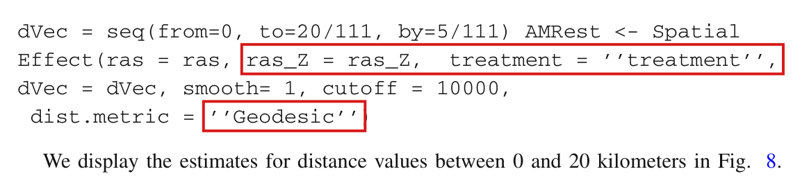
Crop of four lines of code and one line of text. The code is 'dVec = seq(from=0, to=20/111, by=5/111) AMRest <- Spatial', 'Effect(ras = ras, ras_Z = ras_Z, treatment = ''treatment'',', 'dVec = dVec, smooth= 1, cutoff = 10000,' and 'dist.metric = ''Geodesic'')'. Red boxes mark 'ras_Z = ras_Z, treatment = ''treatment'',' and the string ''Geodesic'', each printed between pairs of apostrophes.
Section 6, p. 153 (PDF p. 16), the printed call for the application. The first marked part supplies the polygons and the name of the treatment attribute, and the call has no Zdata. The second marked part shows the paired apostrophes printed in place of quotation marks.
Crop of five lines of text about the option numpts. A red box marks the sentence 'We sample roughly the same number of points for circles with different radius.'
Section 3, p. 145 (PDF p. 8). The marked sentence describes the default number of sampling points on a circle.

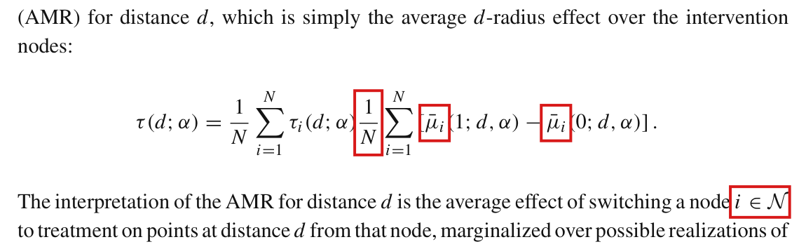
The display of the AMR lacks the equals sign between its two averages and carries bars on μi\mu_i that are not defined: the AMR is τ(d;α)=N−1∑i=1Nτi(d;α)=N−1∑i=1N[μi(1;d,α)−μi(0;d,α)]\tau(d;\alpha)=N^{-1}\sum_{i=1}^N\tau_i(d;\alpha)=N^{-1}\sum_{i=1}^N[\mu_i(1;d,\alpha)-\mu_i(0;d,\alpha)].

Section 2.2, p. 143 (PDF p. 6), display defining τ(d;α)\tau(d;\alpha) and the sentence after it

See also under Formal statements (Lean): P008-T14

As printed
τ(d;α)=1N∑i=1Nτi(d;α) = 1N∑i=1N[μˉi(1;d,α)−μˉi(0;d,α)].\tau(d;\alpha)=\frac{1}{N}\sum_{i=1}^{N}\tau_i(d;\alpha)\,\colorbox{#ffe58a}{$\displaystyle \phantom{=}$}\,\frac{1}{N}\sum_{i=1}^{N}\left[\colorbox{#ffe58a}{$\displaystyle \bar{\mu}_i$}(1;d,\alpha)-\colorbox{#ffe58a}{$\displaystyle \bar{\mu}_i$}(0;d,\alpha)\right].

The interpretation of the AMR for distance dd is the average effect of switching a node i∈N\colorbox{#ffe58a}{$i\in\mathcal{N}$} to treatment on points at distance dd from that node, marginalized over possible realizations of treatment statuses in other intervention nodes.

The problem

The two averages stand side by side with no sign between them, and as printed the display reads as their product. The second average is written with μˉi\bar{\mu}_i, although the page defines only μi(z;d,α)\mu_i(z;d,\alpha). The sentence after the display uses a set N\mathcal{N} that is not defined. By p. 141 it can only be the set {1,…,N}\{1,\ldots,N\} of indices of the intervention nodes.

Evidence a derivation

I derived the identity from the definitions that precede the display. On p. 143 the paper sets τi(d;α)=μi(1;d,α)−μi(0;d,α)\tau_i(d;\alpha)=\mu_i(1;d,\alpha)-\mu_i(0;d,\alpha). Substituting this into the first average, I obtain

1N∑i=1Nτi(d;α)=1N∑i=1N[μi(1;d,α)−μi(0;d,α)],\frac1N\sum_{i=1}^N\tau_i(d;\alpha)=\frac1N\sum_{i=1}^N\left[\mu_i(1;d,\alpha)-\mu_i(0;d,\alpha)\right],

and the two averages are equal. The missing sign is an equals sign. The product is a different quantity. For N=2N=2 with (μ1(1),μ2(1))=(3,7)(\mu_1(1),\mu_2(1))=(3,7) and (μ1(0),μ2(0))=(0,2)(\mu_1(0),\mu_2(0))=(0,2), each average equals 44 and their product is 1616. The estimator on p. 144 is written with μi\mu_i without a bar.

What survives

The AMR as defined in the sentences before the display is unchanged, and so is the Hajek estimator on p. 144. Only the display and the index set after it change.

Corrected

Let μi(z;d,α)=EZ−i[μi(Y(z,Z−i);d)]\mu_i(z;d,\alpha)=\mathrm{E}_{\mathbf{Z}_{-i}}[\mu_i(\mathbf{Y}(z,\mathbf{Z}_{-i});d)] be the potential circle average of radius dd around node ii under the design α\alpha, and let τi(d;α)=μi(1;d,α)−μi(0;d,α)\tau_i(d;\alpha)=\mu_i(1;d,\alpha)-\mu_i(0;d,\alpha), as on p. 143. The AMR for distance dd is

τ(d;α)=1N∑i=1Nτi(d;α)=1N∑i=1N[μi(1;d,α)−μi(0;d,α)].\tau(d;\alpha)=\frac{1}{N}\sum_{i=1}^{N}\tau_i(d;\alpha)\colorbox{#ffe58a}{$\displaystyle =$}\frac{1}{N}\sum_{i=1}^{N}\left[\colorbox{#ffe58a}{$\displaystyle \mu_i$}(1;d,\alpha)-\colorbox{#ffe58a}{$\displaystyle \mu_i$}(0;d,\alpha)\right].

The interpretation of the AMR for distance dd is the average effect of switching a node i∈{1,…,N}\colorbox{#ffe58a}{$i\in\{1,\ldots,N\}$} to treatment on points at distance dd from that node, marginalized over possible realizations of treatment statuses in other intervention nodes.

Crop of the display and the lines around it. The text reads: (AMR) for distance d, which is simply the average d-radius effect over the intervention nodes. The display reads: tau of d and alpha equals one over N times the sum over i from 1 to N of tau i of d and alpha, followed with no sign between them by one over N times the sum over i from 1 to N of the bracket mu-bar i of 1, d, alpha minus mu-bar i of 0, d, alpha. The next line reads: The interpretation of the AMR for distance d is the average effect of switching a node i in calligraphic N. Red outlines surround the second fraction one over N, the two symbols mu-bar i, and the words i in calligraphic N.
Section 2.2, p. 143 (PDF p. 6), display defining the AMR. The outline at the second fraction marks the place of the missing equals sign; the other outlines mark the two bars and the undefined index set.

As printed, the displayed R commands do not parse: two assignments are run together, the name SpatialEffect is split across a line, and the strings are set in typographic quotation marks.

Section 6, displayed SpatialEffect() call, p. 153 (PDF p. 16)

As printed

dVec = seq(from=0, to=20/111, by=5/111) AMRest <- Spatial

Effect(ras = ras, ras_Z = ras_Z, treatment = ’’treatment’’,

dVec = dVec, smooth= 1, cutoff = 10000,

dist.metric = ’’Geodesic’’)

The problem

The assignment to dVec and the assignment to AMRest are printed on one line with no separator, the function name is broken into Spatial and Effect at the line end, and the strings are delimited by pairs of typographic apostrophes. R stops at AMRest. With the two assignments separated and ordinary quotes restored, R still reads AMRest <- Spatial followed by a separate call to Effect().

Evidence an exact counterexample

The evidence is a check of the page and a parse of the printed commands in R, which stops with an “unexpected symbol” error at AMRest. The corrected commands parse as the two intended expressions. No estimation was run.

What survives

The intended commands and the surrounding explanation are unaffected; this is a repair of syntax only. It does not address the grid of distances in the same call, which is the subject of P008-E004.

Corrected

dVec = seq(from=0, to=20/111, by=5/111)

AMRest <- SpatialEffect(ras = ras, ras_Z = ras_Z, treatment = "treatment",

dVec = dVec, smooth= 1, cutoff = 10000,

dist.metric = "Geodesic")

The four printed lines of R code on page 153, with two lines of text above and below. Red boxes mark four items: the assignment to AMRest that ends the first code line with the word Spatial, the word Effect that starts the second line, and the strings treatment and Geodesic, each set between pairs of apostrophes.
Section 6, displayed call, p. 153 (PDF p. 16). The marks show the second assignment run onto the first line, the function name split across the line end, and the two strings set in typographic apostrophes.

Author names are garbled in three reference entries and in one citation in the text: given names are taken as surnames, and one author is split into two.

References, pp. 155–156 (PDF pp. 18–19); in-text citation, p. 140 (PDF p. 3)

As printed

Aronow PM, Dean E, Cyrus S, Stephanie Z (2020) Spillover effects in experimental data. arXiv:2001.05444

Arriagada RA, Ferraro PJ, Erin O, Sills, Pattanayak SK, Cordero-Sancho S (2012) Do payments for environmental services affect forest cover? A farm-level evaluation from costa rica. Land Econ 88(2):382–399.

Hudgens MG, Elizabeth Halloran M (2008) Toward causal inference with interference. J Am Stat Assoc 103(482):832–842

[p. 140] Hudgens and Elizabeth Halloran (2008)

The problem

The first entry gives the coauthors Dean Eckles, Cyrus Samii and Stephanie Zonszein by given name and an initial of the surname. The second splits the single author Erin O. Sills into “Erin O” and “Sills”. The third, and the citation on p. 140, treat “Elizabeth” as part of the surname of M. Elizabeth Halloran.

Evidence a check of the printed page

The evidence is a check of the pages against public author records: the author list of the cited arXiv preprint, the publication record of the Land Economics article and the curriculum vitae of E. O. Sills, and the PubMed record of the article of Hudgens and Halloran together with the curriculum vitae of M. E. Halloran. The journal versions of record of the last two articles were not read.

What survives

The three works remain identifiable from their titles, years and identifiers, and no result of the paper is touched.

Corrected

Aronow PM, Eckles D, Samii C, Zonszein S (2020) Spillover effects in experimental data. arXiv:2001.05444

Arriagada RA, Ferraro PJ, Sills EO, Pattanayak SK, Cordero-Sancho S (2012) Do payments for environmental services affect forest cover? A farm-level evaluation from costa rica. Land Econ 88(2):382–399.

Hudgens MG, Halloran ME (2008) Toward causal inference with interference. J Am Stat Assoc 103(482):832–842

[p. 140] Hudgens and Halloran (2008)

Three entries of the reference list on page 155. Red boxes mark two strings of names: Dean E, Cyrus S, Stephanie Z in the entry for Aronow and coauthors (2020), and Erin O, Sills in the entry for Arriagada and coauthors (2012).
References, p. 155 (PDF p. 18). The marked strings give three coauthors by given name and split Erin O. Sills into two authors; the entry above prints “Samii C” correctly. The entry for Hudgens and Halloran on p. 156 and the citation on p. 140 are not shown.

For d≥kd\ge k, a band between d−kd-k and d+kd+k has width 2k2k, not kk, and the “disk” is the full disc of radius dd, not a sector; in the later archived version of the package the “donut” for polygon interventions is the band between consecutive radii of dVec and is not centered at dd.

Section 2.2, p. 143 (PDF p. 6), sentence beginning “Another option that the SpatialEffect package offers”; Section 3, p. 145 (PDF p. 8), sentence on the option cType

See also under Formal statements (Lean): P008-T16, P008-T17

As printed

p. 143. Another option that the SpatialEffect package offers is to define the circle average as points that are within a kk-coordinate-wide bandwidth around points that are dd coordinate units from the intervention node; this latter specification defines a disc or circular band (or “donut”) of intervention nodes that are between d−kd-k and d+kd+k coordinate units from the intervention node.

p. 145. Users can choose a set of points that form the edge of a circle of radius dd, that form a circular band (“donut”) centered at radius dd, or that form a sector centered at dd (“disk”), by altering the option cType.

The problem

The two sentences describe the band and the disc inexactly, and the description differs from what the available code does.

First, the points within distance kk of the circle of radius dd are the points between max⁡(0,d−k)\max(0,d-k) and d+kd+k from the node. The endpoints on p. 143 are correct when d≥kd\ge k, but this band is 2k2k wide. Then kk is its half-width and not its width.

Second, dd is a radius and not a place, and a sector would need an angle, which neither the text nor the package specifies. The “disk” is the full disc of radius dd around the node. For a polygon it is the polygon together with all points within distance dd of it.

Third, the only archived version of the package that has the option cType is the one distributed with the replication files of Wang, Samii, Chang and Aronow (2024), which is later than the release that the paper cites (version 0.1, 2020). This later version has no argument kk. For polygon interventions, its “donut” at the jjth radius djd_j of dVec, j>1j>1, averages the outcome cells that lie between the buffers of radii dj−1d_{j-1} and djd_j around the polygon, and at the first radius it averages the full buffer. Such a band ends at djd_j and is not centered there. Someone who follows the text would place a donut estimate half a band away from the region it averages. The release that the paper cites is not archived, and I could not determine whether it behaved in the same way.

Evidence an exact counterexample

I derived the width of the band and ran an exact example through the function SpatialEffect() of the later version.

Width. Let rr be the distance of a point xx from the node. By the reverse triangle inequality, every point of the circle of radius dd is at distance at least ∣r−d∣|r-d| from xx, and a radially aligned point of the circle attains this bound. This implies that the points within distance kk of the circle are the points such that max⁡(0,d−k)≤r≤d+k\max(0,d-k)\le r\le d+k. For d=4d=4 and k=1k=1 the band is [3,5][3,5], of width 22.

Example. Let the treated polygon be a small square, let dVec be (2,4)(2,4), and let the only outcome cells near the square lie at distances 00, 19/819/8, 27/827/8 and 35/835/8 from its boundary, with outcomes 44, 22, 00 and 88. Let all outcomes near the control polygon be 00. The buffer of radius 22 contains one cell, with sum 44, and the buffer of radius 44 contains three cells, with sum 66.

The example at the radius 44: the average of the outcome cells of the treated polygon over three regions, with the cells listed by their distance from the boundary of the polygon. The control averages are 00, so each average is also the estimate of the AMR.
RegionCells, by distanceAverage
Between the buffers of radii 22 and 44 (“donut”)19/819/8, 27/827/8(6−4)/(3−1)=1(6-4)/(3-1)=1
Band [3,5][3,5], of the same width, centered at 4427/827/8, 35/835/8(0+8)/2=4(0+8)/2=4
Full buffer of radius 44 (“disk”)00, 19/819/8, 27/827/86/3=26/3=2

The function returns 11 for the donut and 22 for the disk at the radius 44, in agreement with the first and third rows, and not the value 44 of the centered band.

What survives

The corrections of wording change no reported number. The definition of the AMR on exact circles, the estimator and the toy example do not use these options. The bottom panel of Figure 8 uses the donut option, and where its points are drawn is the subject of P008-N017.

Corrected

p. 143. Another option that the SpatialEffect package offers is to define the circle average as points that are within distance kk of the circle of radius dd around the intervention node; this latter specification defines a disc or circular band (or “donut”) of outcome points that are between max⁡(0,d−k)\colorbox{#ffe58a}{$\max(0,d-k)$} and d+kd+k coordinate units from the intervention node, so that kk is the half-width of the band when d≥kd\ge k.

p. 145. Users can choose a set of points that form the edge of a circle of radius dd, that form a circular band (“donut”) centered at radius dd, or that form the full disc of radius dd around the intervention node (“disk”), by altering the option cType. In the later archived version of the package, the donut for polygon interventions is not centered at dd: at the jjth radius djd_j of dVec, j>1j>1, it averages the outcome cells between the buffers of radii dj−1d_{j-1} and djd_j around the polygon, and at the first radius it averages the full buffer.

The words “of outcome points” on p. 143 follow P008-E007.

Crop of six lines of text. The marked sentence reads: Another option that the SpatialEffect package offers is to define the circle average as points that are within a k-coordinate-wide bandwidth around points that are d coordinate units from the intervention node; this latter specification defines a disc or circular band (or donut) of intervention nodes that are between d minus k and d plus k coordinate units from the intervention node. Red outlines surround the words k-coordinate-wide bandwidth and the words between d minus k and d plus k.
Section 2.2, p. 143 (PDF p. 6). The outlines mark the stated width of the band and its endpoints, which are 2k2k apart.
Crop of five lines of text. The marked sentence reads: Users can choose a set of points that form the edge of a circle of radius d, that form a circular band (donut) centered at radius d, or that form a sector centered at d (disk), by altering the option cType. Red outlines surround the words centered at radius d and the words sector centered at d (disk).
Section 3, p. 145 (PDF p. 8), sentence on the option cType. The outlines mark the descriptions of the donut and of the disk.

The intervals printed as spatial-HAC intervals in the toy example contain no covariance between nodes and equal the heteroskedasticity-robust (HC0) intervals, because the cutoff 0.4 is smaller than every distance between the four nodes; they do not follow the rule of Section 3 and do not adjust for interference between nodes.

Section 3, p. 145 (PDF p. 8), the rule for cutoff; Section 5, pp. 147–148 (PDF pp. 10–11), the cutoff of the toy example; p. 149 (PDF p. 12), the columns Conley.CI.l and Conley.CI.u and the description of the red line of Figure 5

See also under Formal statements (Lean): P008-T5, P008-T6, P008-T10, P008-T23

As printed

p. 145. For the asymptotic variance estimator, users need to specify a distance threshold (cutoff) beyond which interference dependence does not exist. This can be based on substantive judgments about the likely spatial extent of interference, and can be varied as part of a sensitivity analysis.

pp. 147–148. The cutoff point for the spatial HAC variance is set to be 0.4 and the number of permutations is set to be 1000.

p. 149. The red dotted line is the 95% confidence interval based on the spatial-HAC standard errors.

The problem

Section 3 asks for a cutoff beyond which interference dependence does not exist. In the toy example the four nodes are between 1.431.43 and 3.403.40 coordinate units apart, and the simulated effect of a node does not vanish over these distances: at distance 22 it is −0.58-0.58. The cutoff 0.4 is below the smallest distance between two nodes, so no pair of distinct nodes enters the variance estimator. The estimator then reduces to the heteroskedasticity-robust (HC0) variance of a difference in means, and all ten printed intervals equal the HC0 intervals to the three decimals shown.

The example presents these intervals as spatial-HAC intervals, in a tutorial on inference under interference, but they contain no adjustment for dependence between nodes. That dependence is present in the reconstruction below. Under the Bernoulli design of the example, the contributions of two distinct nodes to the estimator have positive covariance for every pair of nodes at d=0.1d=0.1, and the sum of these covariances is positive at each of the 20 radii. The rule on p. 145 is correct as written, and the defect lies in the example. A user who chooses cutoff as the example does leaves these covariances out.

Evidence an exact counterexample

The evidence is a recalculation of the toy example from the vignette distributed with the package, and an exact counterexample for the general point.

Recalculation. Starting from the seed and the recipe of the vignette, I obtain the ten printed estimates and the twenty printed endpoints of the intervals, to three decimals. The smallest distance between two nodes is 1.4295>0.41.4295>0.4. With the uniform kernel, the spatial-HAC variance of the estimate is ∑i,jqiqjeiej1{Dij≤0.4}\sum_{i,j}q_iq_je_ie_j\mathbf{1}\{D_{ij}\le 0.4\}, where q=(1/2,1/2,−1/2,−1/2)q=(1/2,1/2,-1/2,-1/2), eie_i is the residual of the circle average of node ii from the mean of its arm, and DijD_{ij} is the distance between nodes ii and jj. Only the terms with i=ji=j remain, and the variance is the HC0 variance ∑iqi2ei2\sum_i q_i^2e_i^2.

The output printed on p. 149 beside the HC0 interval recomputed from the vignette, that is, the estimate plus and minus the 0.9750.975 normal quantile times the HC0 standard error.
ddAMR_est, printedConley.CI, printedHC0 standard errorHC0 interval
0.10.11.4911.491[−0.277, 3.259][-0.277,\ 3.259]0.90200.9020[−0.2772, 3.2586][-0.2772,\ 3.2586]
0.20.21.5501.550[−0.242, 3.343][-0.242,\ 3.343]0.91450.9145[−0.2420, 3.3429][-0.2420,\ 3.3429]
0.30.31.5501.550[−0.242, 3.343][-0.242,\ 3.343]0.91450.9145[−0.2420, 3.3429][-0.2420,\ 3.3429]
0.40.41.6911.691[−0.050, 3.431][-0.050,\ 3.431]0.88800.8880[−0.0497, 3.4313][-0.0497,\ 3.4313]
0.50.51.7141.714[−0.020, 3.448][-0.020,\ 3.448]0.88460.8846[−0.0197, 3.4480][-0.0197,\ 3.4480]
0.60.61.7001.700[−0.038, 3.438][-0.038,\ 3.438]0.88670.8867[−0.0382, 3.4376][-0.0382,\ 3.4376]
0.70.71.6781.678[−0.066, 3.422][-0.066,\ 3.422]0.89000.8900[−0.0664, 3.4224][-0.0664,\ 3.4224]
0.80.81.0021.002[−0.067, 2.071][-0.067,\ 2.071]0.54540.5454[−0.0675, 2.0705][-0.0675,\ 2.0705]
0.90.9−0.816-0.816[−2.424, 0.791][-2.424,\ 0.791]0.82020.8202[−2.4241, 0.7912][-2.4241,\ 0.7912]
1.01.0−0.791-0.791[−2.295, 0.714][-2.295,\ 0.714]0.76760.7676[−2.2955, 0.7136][-2.2955,\ 0.7136]

The covariances left out. Since the effects are additive in the toy example, the circle average of node ii is μi=bi+∑kaikZk\mu_i=b_i+\sum_k a_{ik}Z_k, where aika_{ik} is the average effect of node kk on the circle of node ii. Let m1m_1 and m0m_0 be the averages over the nodes of the marginal circle means under treatment and under control, and let ϕi=2Zi(μi−m1)−2(1−Zi)(μi−m0)\phi_i=2Z_i(\mu_i-m_1)-2(1-Z_i)(\mu_i-m_0) be the contribution of node ii to the linearized Hajek estimator. Under independent Bernoulli(1/21/2) assignment, a direct computation gives

Cov⁡(ϕi,ϕj)=aijaji(i≠j).\operatorname{Cov}(\phi_i,\phi_j)=a_{ij}a_{ji}\qquad(i\ne j).

At d=0.1d=0.1 the twelve coefficients aija_{ij} with i≠ji\ne j are negative, which implies that the six covariances are positive. For nodes 3 and 4, which are 1.431.43 apart, I have a34=−0.9235a_{34}=-0.9235 and a43=−1.1507a_{43}=-1.1507, and the covariance is 1.06271.0627. The variance of the mean of the four ϕi\phi_i at d=0.1d=0.1 is 1.49461.4946 with the covariances and 1.26801.2680 without them. The part left out is positive at each of the 20 radii, between 0.0130.013 and 0.2270.227. Note that these are variances of the linearization under the design, and not the finite-sample variance of the estimator with four nodes. I make no claim about the coverage of the printed intervals.

Counterexample for the general point. A cutoff equal to the range over which a node affects outcomes can be too small. Let two nodes lie at (0,0)(0,0) and (2,0)(2,0), let the outcome points be (−1,0)(-1,0), (1,0)(1,0) and (3,0)(3,0), and let a treated node raise by 11 the outcome of every point within distance 11 of it. Under independent Bernoulli(1/21/2) assignment and for d=1d=1, the circle averages are μ1=Z1+Z2/2\mu_1=Z_1+Z_2/2 and μ2=Z2+Z1/2\mu_2=Z_2+Z_1/2, and the AMR is 11. With Sk=2Zk−1S_k=2Z_k-1, I obtain ϕ1=ϕ2=S1S2/2\phi_1=\phi_2=S_1S_2/2, so that Var⁡(ϕi)=Cov⁡(ϕ1,ϕ2)=1/4\operatorname{Var}(\phi_i)=\operatorname{Cov}(\phi_1,\phi_2)=1/4. The variance of (ϕ1+ϕ2)/2(\phi_1+\phi_2)/2 is 1/41/4, and the terms with i=ji=j contribute 1/81/8. A cutoff of 11 excludes the pair, which is 22 apart, and leaves out half of the variance. The same ratio holds for any number of such pairs placed far from one another.

What survives

The rule on p. 145 is correct, and this cutoff correction leaves the estimates, the permutation bounds and the printed numbers unchanged. The toy intervals are nominal HC0 intervals, and they can no longer be read as adjusted for interference. I have not established an error in the application’s intervals; I could not obtain the package release and the exact transformed inputs used for them. Nor have I established an error in the asymptotic result that the paper attributes to Wang et al. (2022). The application bases its statement of significance on a permutation test, which does not use the cutoff.

Corrected

p. 145. For the asymptotic variance estimator, users need to specify a distance threshold (cutoff) beyond which interference dependence does not exist between the contributions of two intervention nodes to the estimate at the radius being analyzed; this distance can exceed the distance over which a node affects outcomes.

pp. 147–148. The cutoff point for the spatial HAC variance is set to be 0.4 and the number of permutations is set to be 1000. With cutoff 0.4, no distinct pair of intervention nodes enters the variance estimator. The limits displayed as Conley.CI.l and Conley.CI.u equal HC0 limits and do not adjust for interference between nodes; they illustrate nominal intervals and not calibrated inference in this four-node example.

p. 149. The red dotted line is the 95% confidence interval based on the HC0 standard errors, to which the spatial-HAC standard errors reduce at this cutoff.

No other value of the cutoff is proposed for the example. With four nodes, a uniform kernel that includes every pair gives a variance estimate of zero, and a calibrated interval for this example would need a separately justified procedure.

Crop of four lines of text. The marked sentence reads: For the asymptotic variance estimator, users need to specify a distance threshold (cutoff) beyond which interference dependence does not exist. It is followed by: This can be based on substantive judgments about the likely spatial extent of interference, and can be varied as part of a sensitivity analysis. Red outlines surround the words distance threshold (cutoff) beyond which interference dependence does not exist.
Section 3, p. 145 (PDF p. 8). The outlines mark the rule for the choice of cutoff.
Crop of three lines of text and four lines of R code. The text reads: point for the spatial HAC variance is set to be 0.4 and the number of permutations is set to be 1000. We use the SpatialEffect() function to estimate the AMR as follows. The code reads: dVec = seq(from=.1,to=2, by=.1); AMRest <- SpatialEffect(ras = ras\_sim, Zdata = Zdata, x\_coord\_Z = ''x'', y\_coord\_Z = ''y'', treatment = ''Z'', dVec = dVec, cutoff = .4, nPerms = 1000, smooth = 1). Red outlines surround the words point for the spatial HAC variance is set to be 0.4 and the argument cutoff = .4.
Section 5, p. 148 (PDF p. 11), end of the sentence that begins on p. 147, and the call below it. The outlines mark the cutoff 0.4 in the text and in the call.
Crop of a printed table with ten rows and the columns dVec, AMR\_est, Conley.CI.l, Conley.CI.u, Per.CI.l and Per.CI.u, followed by three lines of text. The Conley columns read, for d from 0.1 to 1.0: -0.277 and 3.259; -0.242 and 3.343; -0.242 and 3.343; -0.050 and 3.431; -0.020 and 3.448; -0.038 and 3.438; -0.066 and 3.422; -0.067 and 2.071; -2.424 and 0.791; -2.295 and 0.714. The text below reads: The results are also presented in Fig. 5. The black solid line in the graph is the AMR estimate for each of the distance values d. The red dotted line is the 95\% confidence interval based on the spatial-HAC standard errors. Red outlines surround the column headings Conley.CI.l and Conley.CI.u, the two columns of values, and the sentence about the red dotted line.
Output of summary(), p. 149 (PDF p. 12), and the sentence below it. The outlines mark the two columns of the spatial-HAC interval, which equal the HC0 interval in every row, and the description of the red line of Figure 5.
Figure with two panels. The left panel is a dot plot of the distance between two nodes, in coordinate units from 0 to 4, with one row for each pair: nodes 3 and 4 at 1.43, nodes 1 and 3 at 1.48, nodes 1 and 4 at 2.83, nodes 1 and 2 at 3.32, nodes 2 and 3 at 3.39, and nodes 2 and 4 at 3.40. A vertical line at 0.4 is labelled cutoff 0.4, and the region to its left is shaded and contains no dot. The right panel plots the variance of the linearized estimator, in squared units of the outcome, against the radius d of the circle average from 0.1 to 2.0. A blue line with circles, variances and covariances of the nodes, starts at about 1.49 at d = 0.1, falls to about 0.39 at d = 1.2 and ends at about 0.52 at d = 2.0. An orange line with squares, variances only (all that the cutoff keeps), lies below it at every radius, from about 1.27 at d = 0.1 to about 0.35 at d = 2.0. The band between the two lines is shaded.
The toy example. Left: the six distances between the four nodes, all above the cutoff 0.4, so that no pair enters the variance. Right: the variance of the linearized estimator under the Bernoulli design, with the covariances between nodes and without them, at the 20 radii; the part left out is positive throughout. The curves are variances of the linearization, not finite-sample variances, and they say nothing about coverage.

The right panel of Figure 2 plots a kernel f(d)f(d), and in the toy example a treated node changes the outcome at distance dd by 3f(d)3f(d), three times the plotted curve.

Figure 2, right panel and last sentence of the caption, p. 147 (PDF p. 10)

See also under Formal statements (Lean): P008-T18

As printed

“Figure 2. The plot on the left displays the 4-by-4 raster that records the outcome when treatment is absent (Yx(0)Y_x(0)). Black points are the intervention nodes. The plot on the right presents the non-monotonic effect function.”

Right panel: the vertical axis is labelled “Effect on Yx” and the horizontal axis “Distance from intervention node”. The curve falls from about 1.631.63 at distance 0.10.1 to about −0.55-0.55 near distance 1.21.2, and rises to about −0.19-0.19 at distance 22.

The problem

Section 4 describes the function as “a non-monotonic effect emanating from each intervention node, which is presented on the right plot of Fig. 2”, and the axis of the panel reads “Effect on Yx”. The panel is read as the change in the outcome that one treated node produces at a given distance. Its scale is too small by a factor of three. The plotted curve agrees with the kernel

f(d)=2e−2d−1283 d4e−4d,f(d)=2e^{-2d}-\frac{128}{3}\,d^{4}e^{-4d},

the difference of two gamma densities. The true AMR of Figure 4 and the output table on p. 149 agree with an effect of 3f(d)3f(d) from each treated node. The paper does not state the multiplier.

The mismatch shows in a comparison of two figures. The true AMR in Figure 4 falls to about −1.26-1.26, below the minimum of the plotted function, about −0.55-0.55. When the effects of the nodes add, as they do in the toy data of the package vignette, the AMR is a weighted average of values of the single-node effect and cannot lie below its minimum.

Evidence a derivation

I checked the two figures in the PDF, recalculated the toy example and derived the bound below.

Sixteen points of the curve of Figure 2, read from the drawing in the PDF, agree with ff to within 0.000040.00004. At d=0.1d=0.1 the plotted value is 1.63461.6346, while f(0.1)=1.6346f(0.1)=1.6346 and 3f(0.1)=4.90383f(0.1)=4.9038.

I generated the toy data as in the package vignette, with seed 123567 and the outcome in raster cell cc equal to Y0c+a∑jzjf(rjc)Y_{0c}+a\sum_{j}z_jf(r_{jc}) with a=3a=3, where rjcr_{jc} is the distance from the centre of the cell to node jj. These data reproduce the ten AMR estimates of the printed table and its twenty permutation bounds to the third decimal. Their true AMR under the sixteen Bernoulli assignments agrees with the twenty plotted points of Figure 4 to within 0.00010.0001. At d=1.4d=1.4, Figure 4 shows −1.2578-1.2578; the true AMR is −1.2579-1.2579 with a=3a=3 and −0.4193-0.4193 with a=1a=1. With a=1a=1 the first AMR estimate would be 0.6550.655, and the table prints 1.4911.491.

Averaging does not account for the factor. For outcomes of the form above, the difference between the outcomes with node ii treated and with node ii under control is af(ric)af(r_{ic}), whatever the assignment of the other nodes. Then the AMR at distance dd is ∑i,cwic(d) af(ric)/4\sum_{i,c}w_{ic}(d)\,af(r_{ic})/4, where the weights wic(d)≥0w_{ic}(d)\ge 0 sum to one over cc for each node ii. Let h(r)=(128/3)r4e−4rh(r)=(128/3)r^{4}e^{-4r}. Since h′(r)=(512/3) r3(1−r)e−4rh'(r)=(512/3)\,r^{3}(1-r)e^{-4r}, the maximum of hh on r≥0r\ge 0 is h(1)=128/(3e4)h(1)=128/(3e^{4}), and e4>∑k=064k/k!=437/9e^{4}>\sum_{k=0}^{6}4^{k}/k!=437/9 implies that h(1)<384/437h(1)<384/437. Since f(r)=2e−2r−h(r)f(r)=2e^{-2r}-h(r) and 2e−2r>02e^{-2r}>0, I obtain

f(r)>−384437>−1for all r≥0.f(r)>-\frac{384}{437}>-1\qquad\text{for all } r\ge 0 .

With a=1a=1 the AMR would be above −384/437-384/437 at every distance, and Figure 4 reaches −1.26-1.26.

The script that drew the figures of the paper is not available. The factor 33 is identified by the agreement of the recalculation with the published table and with Figure 4.

What survives

The shape of the curve and the purpose of the illustration are unaffected. No estimate changes: Figures 3 to 5, the printed estimates and intervals, the definitions of Section 2 and the application of Section 6 do not depend on the scale of Figure 2. Only the correspondence between the magnitudes in Figure 2 and those in Figures 3 and 4 changes.

Corrected

“The plot on the right presents the non-monotonic kernel f(d)f(d); in the toy example, each treated node contributes 3f(d)3f(d) to the outcome in a raster cell whose centroid is at distance dd from that node.”

The vertical axis of the right panel is labelled “Kernel f(d)f(d)”, where

f(d)=2e−2d−1283 d4e−4d.f(d)=2e^{-2d}-\frac{128}{3}\,d^{4}e^{-4d}.

Alternatively, the panel keeps the label “Effect on Yx” and plots 3f(d)3f(d), with the values on the vertical axis multiplied by three.

Crop of Figure 2 with its two-line caption. The left panel is a grey 4-by-4 raster titled 'Null raster' with four numbered black nodes. The right panel is a curve that starts near 1.6 at distance 0.1, falls to about minus 0.55 near distance 1.2 and rises to about minus 0.2 at distance 2. Red boxes mark the vertical axis label 'Effect on Yx' and the caption sentence 'The plot on the right presents the non-monotonic effect function.'
Figure 2 and its caption, p. 147 (PDF p. 10). The marked axis label and the marked caption sentence present the curve as the effect on the outcome; its values are one third of the effect used in the toy example.

In Figure 3 the white nodes are treated and the black nodes are under control; the caption exchanges the two colours.

Figure 3 caption, second sentence, p. 148 (PDF p. 11)

As printed

“Figure 3. The plots show the outcome’s values in the raster under each of the sixteen possible assignments. Black nodes are treated and white ones are under control.”

The problem

The second sentence of the caption is the key to the node markers in the sixteen panels, and it is reversed. In panel Z1 all four markers are black, and the panel shows the same raster as the left panel of Figure 2, which records the outcome “when treatment is absent”. Black markers are nodes under control. Panel Z16, with four white markers, shows a different raster. With the printed key, every panel is read with treatment and control exchanged, and a contrast computed by hand from the panels, as in the recipe on p. 147, changes sign.

Evidence a check of the printed page

I checked the page and measured grey levels (0 for black, 255 for white) at the centres of the sixteen cells of each panel in a rendering of the PDF. Panel Z1 differs from the untreated raster of Figure 2 by at most 2 grey levels. Panel Z16 differs from it by more than 5 grey levels in every cell and by as much as 105. With white read as 1, the marker patterns of the sixteen panels are the sixteen binary vectors, from (0,0,0,0)(0,0,0,0) in Z1 to (1,1,1,1)(1,1,1,1) in Z16. The package vignette draws each marker with a grey level equal to the treatment indicator, so that a treated node (Zi=1Z_i=1) is white.

What survives

The coding Zi=1Z_i=1 for a treated node, the rasters shown in Figure 3, the estimands and the estimators are unaffected. No number in the paper depends on the caption.

Corrected

“Figure 3. The plots show the outcome’s values in the raster under each of the sixteen possible assignments. White nodes are treated and black ones are under control.”

Crop of the four panels Z13 to Z16 of Figure 3 and the two-line caption. Each panel is a grey 4-by-4 raster with four numbered round nodes, some black and some white. A red box surrounds panel Z16, in which all four nodes are white. Red boxes also mark the caption words 'Black' and 'nodes are treated and white ones are under control.'
Figure 3, bottom row of panels and caption, p. 148 (PDF p. 11). The marked sentence says that black nodes are treated. In the marked panel Z16 all four nodes are white, and its raster is not the untreated raster of Figure 2.
Crop of the four panels Z1 to Z4 of Figure 3. A red box surrounds panel Z1, in which all four numbered nodes are black. In each of the panels Z2, Z3 and Z4 one node is white and three are black.
Figure 3, top row of panels, p. 148 (PDF p. 11). In the marked panel Z1 all four nodes are black, and its raster is the untreated raster shown in the left panel of Figure 2.

The older archived copy of the SpatialEffect package does not reproduce the twenty endpoints of the spatial-HAC intervals in the toy table; the printed endpoints are matched by a regression of the four circle averages on an intercept and the treatment indicator, with the spatial-HAC variance computed across nodes.

Output table, columns Conley.CI.l and Conley.CI.u, p. 149 (PDF p. 12); red lines of Figure 5, p. 150 (PDF p. 13)

As printed
Output table of the toy example, p. 149.
dVecAMR_estConley.CI.lConley.CI.uPer.CI.lPer.CI.u
0.10.11.4911.491−0.277-0.2773.2593.259−1.566-1.5661.5661.566
0.20.21.5501.550−0.242-0.2423.3433.343−1.626-1.6261.6261.626
0.30.31.5501.550−0.242-0.2423.3433.343−1.626-1.6261.6261.626
0.40.41.6911.691−0.050-0.0503.4313.431−1.666-1.6661.6661.666
0.50.51.7141.714−0.020-0.0203.4483.448−1.684-1.6841.6841.684
0.60.61.7001.700−0.038-0.0383.4383.438−1.673-1.6731.6731.673
0.70.71.6781.678−0.066-0.0663.4223.422−1.657-1.6571.6571.657
0.80.81.0021.002−0.067-0.0672.0712.071−1.005-1.0051.0051.005
0.90.9−0.816-0.816−2.424-2.4240.7910.791−1.328-1.3281.3281.328
1.01.0−0.791-0.791−2.295-2.2950.7140.714−1.307-1.3071.3071.307
The problem

The paper cites version 0.1 of the package (Samii and Wang 2020), which is not available. The archived repository of the package holds two copies of the code: an older copy at its top level and a later copy in the folder of a 2024 replication. Run on the toy data, the older copy returns the ten AMR estimates and the twenty permutation bounds of the printed table, and none of its twenty spatial-HAC endpoints. At d=0.1d=0.1 it gives [0.127, 2.855][0.127,\,2.855], where the table prints [−0.277, 3.259][-0.277,\,3.259]. The largest difference in an endpoint is 0.8660.866, at d=0.5d=0.5. The difference bears on the test of the weak null: the lower endpoints from the older copy are positive at the first seven distances, and the printed ones are negative.

The cause is the covariance. The older copy computes it from a regression on the sampled raster outcomes, 499 rows with the coordinates of the raster cells. A regression on the four circle averages, with the coordinates of the nodes, reproduces the printed intervals. The older copy also cannot run the printed call as it stands: its SpatialEffect() has no smooth argument and no ras_Z argument, and the copy has no SpatialEffectTest().

Nothing printed is shown to be wrong. The finding is that the table cannot be reproduced from this archived copy.

Evidence a recalculation from the source

The evidence is a recalculation from the code. I generated the toy data as in the package vignette (seed 123567), with observed assignment Z=(1,1,0,0)Z=(1,1,0,0), and ran the older copy without the smooth argument and with the name that the vignette gives to the treatment column.

The printed intervals are recovered as follows. For a distance dd, let μi\mu_i be the circle average of node ii, and consider the regression of μ1,…,μ4\mu_1,\dots,\mu_4 on the rows Xi=(1,Zi)X_i=(1,Z_i). The coefficient of ZiZ_i is the AMR estimate τ^(d)=(μ1+μ2−μ3−μ4)/2\widehat{\tau}(d)=(\mu_1+\mu_2-\mu_3-\mu_4)/2. With B=(X⊤X)−1B=(X^{\top}X)^{-1}, residuals ee, and the uniform kernel Kij=1{∥x(i)−x(j)∥<0.4}K_{ij}=\mathbf{1}\{\lVert x(i)-x(j)\rVert<0.4\} on the node coordinates, the spatial-HAC covariance without a degrees-of-freedom correction is BX⊤{K∘(ee⊤)}XBBX^{\top}\{K\circ(ee^{\top})\}XB. Since the smallest distance between two nodes is 1.431.43, the matrix KK is the identity, and the variance of τ^(d)\widehat{\tau}(d) is

V(d)=(μ1−μ2)2+(μ3−μ4)28.V(d)=\frac{(\mu_1-\mu_2)^2+(\mu_3-\mu_4)^2}{8}.

The interval is τ^(d)±Φ−1(0.975)V(d)\widehat{\tau}(d)\pm\Phi^{-1}(0.975)\sqrt{V(d)}. At d=0.1d=0.1 the circle averages are

(μ1,μ2,μ3,μ4)=(−0.5941, 1.8588, −1.2093, −0.5076),(\mu_1,\mu_2,\mu_3,\mu_4)=(-0.5941,\ 1.8588,\ -1.2093,\ -0.5076),

and I find τ^=1.4907\widehat{\tau}=1.4907 and the interval [−0.2772, 3.2586][-0.2772,\,3.2586]. Together with the AMR and permutation calculations, this reproduces all 50 printed cells of the table to the third decimal.

Spatial-HAC intervals of the toy example: as printed, from the older archived copy, and from the calculation on the four nodes.
ddPrintedOlder copyCalculation on nodes
0.10.1[−0.277, 3.259][-0.277,\ 3.259][0.127, 2.855][0.127,\ 2.855][−0.277, 3.259][-0.277,\ 3.259]
0.20.2[−0.242, 3.343][-0.242,\ 3.343][0.296, 2.805][0.296,\ 2.805][−0.242, 3.343][-0.242,\ 3.343]
0.30.3[−0.242, 3.343][-0.242,\ 3.343][0.524, 2.577][0.524,\ 2.577][−0.242, 3.343][-0.242,\ 3.343]
0.40.4[−0.050, 3.431][-0.050,\ 3.431][0.768, 2.614][0.768,\ 2.614][−0.050, 3.431][-0.050,\ 3.431]
0.50.5[−0.020, 3.448][-0.020,\ 3.448][0.846, 2.582][0.846,\ 2.582][−0.020, 3.448][-0.020,\ 3.448]
0.60.6[−0.038, 3.438][-0.038,\ 3.438][0.799, 2.601][0.799,\ 2.601][−0.038, 3.438][-0.038,\ 3.438]
0.70.7[−0.066, 3.422][-0.066,\ 3.422][0.680, 2.676][0.680,\ 2.676][−0.066, 3.422][-0.066,\ 3.422]
0.80.8[−0.067, 2.071][-0.067,\ 2.071][−0.527, 2.530][-0.527,\ 2.530][−0.067, 2.071][-0.067,\ 2.071]
0.90.9[−2.424, 0.791][-2.424,\ 0.791][−3.185, 1.553][-3.185,\ 1.553][−2.424, 0.791][-2.424,\ 0.791]
1.01.0[−2.295, 0.714][-2.295,\ 0.714][−2.907, 1.325][-2.907,\ 1.325][−2.295, 0.714][-2.295,\ 0.714]

The two formulas for the covariance are different, and an exact example shows it. Let every raster outcome equal 11, with the sampled cells of the toy example at d=0.1d=0.1. Then the circle averages all equal 11 and the variance on the nodes is 00, while the formula of the older copy gives 31/4931/49.

What survives

The printed table stands in all 50 cells. The definitions and the asymptotic discussion of Section 2.3 are not affected. The printed cumulative test does not use the spatial-HAC covariance. Which code produced the table is not established. This check does not concern the later copy, whose spatial-HAC calculation is the subject of P008-E015.

Corrected

The printed table needs no change. A statement of the calculation that reproduces its spatial-HAC columns is as follows.

For each distance dd, regress the four circle averages μi(d)\mu_i(d) on an intercept and ZiZ_i. Let XX be the 4×24\times 2 matrix with rows (1,Zi)(1,Z_i), let ee be the vector of residuals, and let Kij=1{∥x(i)−x(j)∥<cutoff}K_{ij}=\mathbf{1}\{\lVert x(i)-x(j)\rVert<\texttt{cutoff}\} for the node coordinates x(i)x(i), with cutoff=0.4\texttt{cutoff}=0.4. The covariance is

(X⊤X)−1X⊤{K∘(ee⊤)}X(X⊤X)−1,(X^{\top}X)^{-1}X^{\top}\{K\circ(ee^{\top})\}X(X^{\top}X)^{-1},

with no degrees-of-freedom correction. Let V(d)V(d) be its diagonal entry for ZiZ_i. The interval is τ^(d)±Φ−1(0.975)V(d)\widehat{\tau}(d)\pm\Phi^{-1}(0.975)\sqrt{V(d)}, where τ^(d)\widehat{\tau}(d) is the AMR estimate. In the older archived copy, this calculation replaces the covariance computed from the sampled raster outcomes, and the argument smooth is omitted.

Crop of the printed output table with ten rows and the columns dVec, AMR_est, Conley.CI.l, Conley.CI.u, Per.CI.l and Per.CI.u. One red box marks the two column names Conley.CI.l and Conley.CI.u. Two more red boxes mark the ten values under each, from minus 0.277 to minus 2.295 and from 3.259 to 0.714.
Output table, p. 149 (PDF p. 12). The marked columns are the lower and upper endpoints of the spatial-HAC intervals, which the older archived copy of the package does not return.

Neither archived copy of the SpatialEffect package runs the printed toy call with smooth = 1, so the dashed curve of Figure 5 cannot be regenerated from that call.

Figure 5, black dashed curve and caption, p. 150 (PDF p. 13); the call with smooth = 1, p. 148 (PDF p. 11)

As printed

p. 148:

dVec = seq(from=.1,to=2, by=.1)

AMRest <- SpatialEffect(ras = ras_sim, Zdata = Zdata, x_coord_Z = ’’x’’,

y_coord_Z = ’’y’’, treatment = ’’Z’’, dVec = dVec,

cutoff = .4, nPerms = 1000, smooth = 1)

p. 150, Figure 5 caption: “The black dashed line is the smoothed AMR estimates (Color figure online).”

The problem

The printed call requests smoothed estimates, and Figure 5 shows them as the dashed curve. The paper cites version 0.1 of the package (Samii and Wang 2020), which is not available. The archived repository of the package holds two copies of the code: an older copy at its top level and a later copy in the folder of a 2024 replication. Neither runs the printed call.

In the older copy, SpatialEffect() has no argument smooth, and R stops with “unused argument (smooth = 1)”. The later copy accepts the argument and, with its default settings, chooses the two smoothing bandwidths by cross-validation over a grid whose first value is (2−0.1)/10=0.19(2-0.1)/10=0.19. At the first evaluation distance, 0.10.1, the triangular weights with this bandwidth are positive only at the distances 0.10.1 and 0.20.2. The bias-corrected fit is a regression on six columns that include a quadratic term, and two distinct distances do not determine a quadratic. The matrix to be inverted has rank at most four, whatever the outcomes, and R stops with “system is computationally singular”. A call that stops in this step returns nothing, including the unsmoothed estimates it has already computed.

It is not shown that the published dashed curve is wrong, or that the cited release failed.

Evidence an exact counterexample

The evidence is an exact computation and a run of the code. Let t=d−0.1t=d-0.1 and let the design have the columns (1, Z, t, Zt, t2, (Zt)2)(1,\ Z,\ t,\ Zt,\ t^{2},\ (Zt)^{2}), as in the later copy. On the rows with positive weight, I have t∈{0, 1/10}t\in\{0,\,1/10\} and hence t2=t/10t^{2}=t/10. Further, (Zt)2=Zt2(Zt)^{2}=Zt^{2} because ZZ is binary. The vectors

v1=(0, 0, −1/10, 0, 1, 0)⊤,v2=(0, 0, 0, −1/10, 0, 1)⊤v_1=(0,\,0,\,-1/10,\,0,\,1,\,0)^{\top},\qquad v_2=(0,\,0,\,0,\,-1/10,\,0,\,1)^{\top}

therefore satisfy Xv1=Xv2=0Xv_1=Xv_2=0 for the design matrix XX restricted to those rows. For the diagonal matrix WW of their weights, this implies that X⊤WXv1=X⊤WXv2=0X^{\top}WXv_1=X^{\top}WXv_2=0, and the 6×66\times 6 matrix X⊤WXX^{\top}WX has rank at most four. In exact arithmetic, I find rank four and determinant zero for the treatment patterns that occur in the cross-validation folds. The four-column matrix of the linear fit is invertible.

I ran the smoothing functions of the later copy unchanged on an example with four nodes and the distances 0.1,0.2,…,2.00.1,0.2,\dots,2.0, and supplied the variables that the cross-validation function reads from its environment. The run stops with “system is computationally singular: reciprocal condition number = 4.71786e-22”. With both bandwidths set to 0.40.4, the smoother returns finite estimates at all twenty distances for this example, with the bias correction and without smoothed standard errors. I did not make a complete run of the printed call with these bandwidths on the toy data.

What survives

The definitions, the unsmoothed estimator, the solid curve of Figure 5, the output table and its intervals are not affected. The printed test SpatialEffectTest(AMRest, c(0.1, 0.5)) uses the unsmoothed estimates and does not need the dashed curve. No published number is shown to be wrong.

Corrected

The caption needs no change. To obtain smoothed estimates from the later archived copy on the grid 0.1,0.2,…,2.00.1,0.2,\dots,2.0, both bandwidths have to be supplied, through the arguments bw and bw_debias, with bw>0.1\colorbox{#ffe58a}{$\texttt{bw}>0.1$} for the linear fit and bw_debias>0.2\colorbox{#ffe58a}{$\texttt{bw\_debias}>0.2$} for the quadratic bias correction. Each fit needs at least two and three distinct positive-weight distances, respectively, in each treatment group, including at the ends of the grid. Supplying bw alone still starts the cross-validation. In the code, the cross-validation should discard a bandwidth for which X⊤WXX^{\top}WX is not of full rank before the inversion.

The bandwidths used for Figure 5 are not known. To reproduce the dashed curve one needs the release used for the paper and its smoothing settings.

Crop of the four-line caption of Figure 5. Red boxes mark the sentence 'The black dashed line is the smoothed AMR estimates', which ends on the last line before '(Color figure online)'.
Figure 5 caption, p. 150 (PDF p. 13). The marked sentence identifies the dashed curve as the smoothed AMR estimates.
Crop of four lines of code and two lines of text. The code is 'dVec = seq(from=.1,to=2, by=.1)' followed by the call 'AMRest <- SpatialEffect(...)' over three lines. A red box marks the last argument, 'smooth = 1'.
Section 5, p. 148 (PDF p. 11), the printed call for the toy example. The marked argument requests the smoothed estimates.

The value at distance 0 in the edge-based panels of Figure 8 summarizes raster cells on the village boundary, not the area inside the village.

Section 6, first paragraph, p. 153 (PDF p. 16); Figure 8, top panels, p. 154 (PDF p. 17)

See also under Formal statements (Lean): P008-T19, P008-T20

As printed

We consider the experiment as an example of polygon interventions. Therefore, the starting point at 0 corresponds to the area within the boundary of each village.

The problem

The sentence says that the estimate at distance 0 summarizes outcomes over the whole village polygon. The two top panels of Figure 8 show edge estimates: at each distance dd they average the raster cells at distance dd from the village boundary. At d=0d = 0 these are the cells on the inner boundary of the rasterized polygon, and the cells in its interior are left out. The smoothed curve is fitted to these boundary summaries across distances. Its value at 0 is not a contrast over the village area either.

Evidence an exact counterexample

The evidence is an exact counterexample and a recalculation. In the 2024 version of the package source, the default circle type, the edge, keeps only the boundary cells of the rasterized buffer, including at distance 0. I consider a raster of 200 cells with two polygons of 5×55 \times 5 cells, one treated and one control, and I set the outcome to 1 on the nine central cells of the treated polygon and to 0 elsewhere. The edge estimate at distance 0 uses the 16 boundary cells of each polygon and equals 0/16−0/16=00/16 - 0/16 = 0, while the contrast over the polygon areas is 9/25−0/25=9/259/25 - 0/25 = 9/25.

On the unaggregated forest-loss raster and the 121 village polygons in the replication files of the later companion paper, the boundary contrast is −0.010516-0.010516 and the contrast inside the villages is −0.013466-0.013466. The boundary value is about 21.9%21.9\% smaller in magnitude. These two values agree visually with the left end of the Hajek curve and with the first step of the bottom panel of Figure 8. The inputs and the package release used for the published figure are not archived, and these files are not shown to be the ones behind it. No such percentage is established for the smoothed curve.

What survives

The estimator, the plotted estimates, the confidence intervals and the band estimates of the bottom panel are unchanged; only the description of the point at 0 changes. The test over 1–2.5 km uses only the distances in that window and does not involve this point.

Corrected

For the edge-based estimates, the value at distance 0 averages outcomes over raster cells on the village boundary, rather than over the full village polygon. The smoothed curve is fitted to these boundary-based summaries across distances. In the bottom panel, the first value is the contrast over the area within the village polygons.

Five lines of text from page 153. A red box marks the words: the area within the boundary of each village. They end the sentence that begins: Therefore, the starting point at 0 corresponds to.
Section 6, first paragraph, p. 153 (PDF p. 16). The marked phrase describes the point at distance 0 as the area inside each village; the edge estimates at 0 use the cells on the village boundary.

The horizontal steps in the bottom panel of Figure 8 place the 2 km band estimates and their confidence intervals over the next band out, and the contrast inside the villages over 0–2 km.

Figure 8, bottom panel (“2km Donut Estimates with CIs”), p. 154 (PDF p. 17); description on p. 153 (PDF p. 16)

As printed

[Description of Figure 8, bottom panel, “2km Donut Estimates with CIs”: a step trace with ten horizontal steps. The step over 0–2 km has height about −0.0135-0.0135, the step over 2–4 km about −0.0085-0.0085, the step over 4–6 km about −0.0059-0.0059, the step over 6–8 km about −0.0024-0.0024, the step over 8–10 km about −0.0010-0.0010, and so on to 18–20 km. The last value, about 0.00040.0004, appears only as the end of the vertical stroke at 20 km.]

[p. 153] The bottom graph shows 2km “donut” estimates: we estimate the AMR using outcome raster outcomes within 2km bands, rather than values precisely at the edge of the circle. The results show a similar pattern as the two graphs above.

The problem

The panel is titled as estimates for 2 km bands, and the text says that the AMR is estimated from outcomes within 2 km bands. The step drawn over 2–4 km therefore reads as the estimate for points between 2 and 4 km from a village boundary. It is the estimate for the band from 0 to 2 km. For d=2,4,…,18d = 2, 4, \dots, 18 km, the value is indexed by the outer edge dd of its band (d−2,d](d-2, d] and is then drawn to the right of dd, over [d,d+2][d, d+2]. The value drawn over 0–2 km is the contrast inside the villages, and the estimate for the band from 18 to 20 km has no horizontal step. Both confidence-interval traces are shifted in the same way. The text does not state this convention, and Section 3 describes a band as centred at dd (p. 145). The misplaced spans make the village-interior contrast appear just outside the villages and put each exterior-band step 2 km farther out.

Evidence a recalculation from the source

I compared the published figure with band contrasts recalculated from the forest-loss raster and the 121 village polygons (60 treated, 61 control) in the replication files of the later companion paper, using nested buffers around each village. Matching the eleven heights read from the panel’s vector paths to the recalculated contrasts with the same index dd, I find a root-mean-square discrepancy of 0.0000520.000052, compared with 0.0023070.002307 for matching the ten horizontal steps to the bands they span, a factor of 44 larger. The vector paths show that each horizontal step runs to the right from dd to d+2d + 2, for the estimates and for both confidence-interval traces. The replication files are those of a later paper and have not been shown to be the inputs of the published figure; the table shows the small differences that remain.

Each outcome region, the interval over which the bottom panel of Figure 8 draws its estimate, the height read from the published panel, and the contrast recalculated from the replication files.
BandDrawn overHeight in Figure 8Recalculated
Inside the village0–2 km−0.013466-0.013466−0.013466-0.013466
(0,2](0,2] km2–4 km−0.008476-0.008476−0.008468-0.008468
(2,4](2,4] km4–6 km−0.005939-0.005939−0.005851-0.005851
(4,6](4,6] km6–8 km−0.002395-0.002395−0.002439-0.002439
(6,8](6,8] km8–10 km−0.000958-0.000958−0.000866-0.000866
(8,10](8,10] km10–12 km−0.000212-0.000212−0.000246-0.000246
(10,12](10,12] km12–14 km0.0003550.0003550.0003170.000317
(12,14](12,14] km14–16 km0.0012800.0012800.0013130.001313
(14,16](14,16] km16–18 km0.0002310.0002310.0001790.000179
(16,18](16,18] km18–20 km0.0016730.0016730.0016580.001658
(18,20](18,20] kmend of the stroke at 20 km0.0004080.0004080.0003380.000338
What survives

The heights of the estimates and of the confidence intervals can be kept: for d=2,4,…,20d = 2, 4, \dots, 20 km, dd is the outer edge of the band, while d=0d = 0 denotes the village interior. The two top panels of Figure 8, the test over 1–2.5 km, the method and the toy example do not depend on this drawing convention; this correction does not by itself change the separate spillover-distance conclusion. The existing horizontal steps for the exterior bands move in by 2 km; the final band gains a horizontal step, and the village-interior contrast is shown separately.

Corrected

[Figure 8, bottom panel, redrawn: for d=2,4,…,20d = 2, 4, \dots, 20 km, the estimate for the band (d−2,d](d-2, d] and its confidence interval are drawn over (d−2,d](d-2, d]. The estimate at d=0d = 0 is shown separately, as the contrast inside the villages.]

Caption, added: Each step of the bottom panel is the estimate for the 2 km band of distances that it spans. The value at d=0d = 0 is shown separately as the contrast inside the village polygons.

The bottom panel of Figure 8, titled 2km Donut Estimates with CIs: a black step trace of AMR estimates rising from about -0.013 at the left to about zero at 20 km, between two red dotted confidence-interval traces. Red boxes mark the first horizontal step, drawn over 0 to 2 km, and the short vertical stroke at 20 km where the trace ends.
Figure 8, bottom panel, p. 154 (PDF p. 17). The marked step over 0–2 km is the contrast inside the villages, and every later step is the estimate for the band before it; the estimate for 18–20 km appears only as the marked end of the stroke at 20 km.
Step plot of AMR estimates against distance from the village boundary, 0 to 20 km, with a shaded region at the left for the inside of the village. A dashed orange trace reproduces the published steps. A solid blue trace places the ten exterior-band heights over their own bands and the village-interior height over the shaded region. Ten open circles show recalculated contrasts at the band midpoints, and an eleventh shows the village-interior contrast in the shaded region. The circles closely follow the solid blue trace.
The heights of the bottom panel of Figure 8 as drawn (dashed) and over their corresponding regions (solid), with the contrasts recalculated from the replication files of the later companion paper (circles). The recalculated contrasts closely follow the solid trace; the published value for 18–20 km has no horizontal step.

Clarity notes

Imprecise or ambiguous wording whose intended meaning is correct; not an error.

The numbers δ/2\delta/2 and 1−δ/21-\delta/2, and 0.0250.025 and 0.9750.975, are quantile levels on the probability scale; as percentiles they are the 2.5th and the 97.5th for δ=0.05\delta=0.05.

Section 3, description of Per.CI, p. 146 (PDF p. 9); Section 5 and Figure 5 caption, pp. 149–150 (PDF pp. 12–13); Section 6 and Figure 8 caption, pp. 153–154 (PDF pp. 16–17)

As printed

p. 146: “For a specified error rate of δ\delta (e.g., δ=0.05\delta = 0.05), it is the δ/2\delta/2 and 1−δ/21-\delta/2 percentiles of the sharp null distribution generated by permutation. At each distance dd, the sharp null hypothesis of no effect is rejected if the AMR estimate is smaller than the δ/2\delta/2 percentile or larger than the 1−δ/21-\delta/2 percentile.”

p. 149: “The blue dotted line shows the 0.025 and .975 percentiles of the sharp null permutation distribution.” On the same page: “slightly larger than the .975 percentile of the sharp null permutation distribution” and “The 0.025 and .975 percentiles of the sharp null permutation distribution of the cumulative effect are −7.97-7.97 and 7.977.97”.

p. 150, Figure 5 caption: “the 0.025 and 0.975 percentiles of the sharp null permutation distribution.”

p. 153: “the 0.025 and .975 percentiles of the sharp null permutation distribution are −0.0304-0.0304 and 0.03360.0336”.

p. 154, Figure 8 caption: “the 0.025 and .975 percentiles of the sharp null permutation distribution.”

Intended meaning

The passages give quantile levels on the probability scale and call them percentiles. A percentile rank is 100 times the level. Read literally, the ranks .025 and .975 are 100 times smaller than the ranks 2.5 and 97.5 that are meant. The intended meaning is clear from the context. The error rate is δ=0.05\delta=0.05, and Section 2.3 (p. 144) names the same cutoffs correctly as “the δ/2\delta/2 and 1−δ/21-\delta/2 quantiles of the null permutation distribution”. The legend of Figure 8 reads “Quantiles of sharp null distribution”, and both copies of the code in the archived repository of the package compute the cutoffs with the R function quantile at the levels alpha/2 and 1-alpha/2. For δ=0.05\delta=0.05 these are the 2.5th and 97.5th percentiles.

This note concerns the label only. No reported cutoff was recomputed for it, and it does not address whether a test based on these cutoffs has level δ\delta, which is the subject of P008-E002.

Corrected

Replace “percentiles” by “quantiles” at each of the places quoted: “the δ/2\delta/2 and 1−δ/21-\delta/2 quantiles” and “the δ/2\delta/2 quantile or … the 1−δ/21-\delta/2 quantile” on p. 146, “the .975 quantile” on p. 149, “the 0.025 and .975 quantiles” on pp. 149, 153 and 154, and “the 0.025 and 0.975 quantiles” on p. 150. An equivalent repair keeps the word and multiplies the levels by 100: “the 2.5th and 97.5th percentiles”.

The decision rule in the second sentence on p. 146 is corrected separately in P008-E002.

Crop of eight lines of text from the description of the output of the SpatialEffect command. Red boxes mark the word 'percentiles' after 'the delta over 2 and 1 minus delta over 2', and the word 'percentile' twice in the next sentence, 'smaller than the delta over 2 percentile or larger than the 1 minus delta over 2 percentile'.
Section 3, p. 146 (PDF p. 9), the description of Per.CI. The three marked words name the levels δ/2\delta/2 and 1−δ/21-\delta/2 as percentiles.
Crop of six lines of text. Red boxes mark '0.025 and .975' at the end of one line and 'percentiles' at the start of the next, in the sentence 'The blue dotted line shows the 0.025 and .975 percentiles of the sharp null permutation distribution'.
Section 5, p. 149 (PDF p. 12), the description of Figure 5. The marked words give the levels 0.0250.025 and .975.975 and call them percentiles.

Formal statements (Lean)

Formal results: 16 whole; 10 restricted; 1 refuted; 1 omitted.

Coverage concerns the identified claim under its stated assumptions. A checked proof establishes the formal statement; correspondence to the published text was reviewed by AI. Repository access is currently required to open the source links.

Each result links to its current formal statement and proof. “Whole” covers the identified claim under its assumptions; “restricted” covers the stated narrower scope; “refuted” gives a counterexample to the identified assertion; “omitted” has no current theorem. Any named published theorem used as a premise remains an assumption. Browse the formal results for this work.

Section 6, the permutation test of the cumulative effect between 1 and 2.5 km (the printed SpatialEffect() and SpatialEffectTest() calls, the two percentiles, and “thus significant with p<0.05p < 0.05”), read as the sharp-null randomization test of the experiment: exact examples in which the law of unrestricted permutations is not the law of the design

p. 153 (PDF p. 16); the design sentences on p. 151 (PDF p. 14), p. 145 (PDF p. 8) and p. 142 (PDF p. 5)

p. 153 (PDF p. 16); the design sentences on p. 151 (PDF p. 14), p. 145 (PDF p. 8) and p. 142 (PDF p. 5). The fixed labelled 121-node example and two four-node examples refute the reading that an observed assignment and its treated count identify the design reference law; unrestricted and blocked tails differ in either direction. Restricted: Retains the explicitly labelled 121-node observation and its within-count swap, both normalized supports, and both directions of the four-node tail discrepancy. Does not quantify over every initial 60-treated observed assignment or assert the existence of a relabelling that puts it into the recorded observation form.

Historical component credits
  • Counterexample proved AronowAudit.P008.observed_count_does_not_identify_law Historical support retained; baseline fidelity: ok; manifest: used; used in Solution; Zero-based treated subsets are equivalent to the target’s labelled binary vectors. This refutes uniqueness of the reference law, without claiming to reconstruct the Uganda p-value.
  • Counterexample proved AronowAudit.P008.reference_laws_counterexample Historical support retained; baseline fidelity: ok; manifest: used; used in Solution; A witness for failure of reference-law identification, not a counterexample to the reported empirical numbers. Inclusive absolute tails and uniform weights match the target.
  • Proved AronowAudit.P008.six_support Historical support retained; baseline fidelity: ok; manifest: used; used in Solution; Auxiliary support certification; uniform probabilities enter through uniformLaw in the tail calculations.
  • Proved AronowAudit.P008.blocked_support Historical support retained; baseline fidelity: ok; manifest: used; used in Solution; Auxiliary support certification for T1(B), not a standalone refutation or a law-calculation claim.

Section 6, the claim “The cumulative effect between 1 km and 2.5 km is thus significant with p<0.05p < 0.05”, corrected (formal content: when the percentiles of a permutation distribution give a valid sharp-null test)

p. 153 (PDF p. 16); with p. 151 (PDF p. 14), p. 145 (PDF p. 8), p. 144 (PDF p. 7) and p. 142 (PDF p. 5)

p. 153 (PDF p. 16); with p. 151 (PDF p. 14), p. 145 (PDF p. 8), p. 144 (PDF p. 7) and p. 142 (PDF p. 5). Inclusive tails are calibrated under the actual finite design and conditional laws, common Bernoulli designs become uniform given their count, and the spatial sharp-null statistic is imputable under the stated restrictions. Restricted: The spatial cumulative-test component is confined to Euclidean circles in a measurable whole field, with integrability for every assignment on every evaluated circle; positive finite circle mass and nonempty arms on the positive-probability conditional support make its averages and ratios meaningful. Imputability is asserted for the cumulative statistic on that support, rather than separately for each circle mean. The documentary seven-lottery design, its identification with a particular conditional reference law, and the empirical significance/withdrawal conclusions are not formalized. General finite-law calibration, conditioning, Bernoulli-given-count uniformity and both directions of the four-node law discrepancy are retained.

Historical component credits
  • Proved AronowAudit.P008.design_tail_valid Historical support retained; baseline fidelity: ok; manifest: used; used in Solution; The target itself states the arbitrary-statistic theorem. Inclusive ties give a level bound rather than equality, exactly as claimed.
  • Proved AronowAudit.P008.conditional_tail_valid Historical support retained; baseline fidelity: ok; manifest: used; used in Solution; The target itself states the arbitrary-statistic conditional-law theorem; a sharp-null hypothesis is not missing from this component.
  • Proved AronowAudit.P008.bernoulli_given_count_uniform Historical support retained; baseline fidelity: ok; manifest: used; used in Solution; The open interval 0<p<1 is explicitly in the target, so excluding p=0,1 is faithful. M=0,N are included; no division by a zero count-event probability occurs.
  • Proved AronowAudit.P008.prob_mono Historical support retained; baseline fidelity: ok; manifest: used; used in Solution; Auxiliary monotonicity is already used inside the exported calibration theorem.
  • Proved AronowAudit.P008.sharp_null_cumulative_test_valid Limited support; baseline fidelity: narrower; manifest: used; used in Solution; {'source': 'adjudication+second review', 'adjudicator': 'P008/P008_Audit.lean:3831 requires MeasurableSet P.field, although T2(a) requires sharp-null imputability and calibration under the actual conditional design law, without global field measurability. Adding a non-Borel set disjoint from the finitely many relevant circles preserves their positive finite masses, integrable outcomes, sharp null and cumulative statistic, but violates this hypothesis. The definitions of Plane and circle at P008/P008_Audit.lean:88 and :101 also fix Euclidean distance, omitting other well-defined metrics permitted by S4; neither restriction is cured by the more general calibration declaration elsewhere.', 'suggested_fix': 'Parameterize the spatial model by the chosen metric and replace whole-field measurability by local measurability or a suitable almost-everywhere support condition for the circles actually used. Retain the sharp null, meaningful-average conditions and actual conditional design law.', 'second_review': "P008/P008_Audit.lean:3829 requires the whole field to be measurable at :3831 and uses the Euclidean circles defined at :101. T2(a)'s sharp-null cumulative calibration under the actual conditional design does not require global field measurability or Euclidean distance: a non-Borel addition outside all evaluated circles leaves meaningful circle averages and the statistic unchanged. These assumptions exclude allowed spatial models, even though conditionalLaw at P008/P008_Audit.lean:1603 correctly represents the actual conditional law. Generalize the metric and require only the local regularity needed for the relevant averages and sharp-null imputability.", 'severity': 'major'}

Sections 2.3, 3 and 5: the rule that rejects the sharp null when the statistic lies outside the δ/2\delta/2 and 1−δ/21-\delta/2 percentiles of the null permutation distribution, as an error-rate-δ\delta test (“approximately in exact finite samples”), and its use in the toy example with six assignments

p. 144 (PDF p. 7); p. 146 (PDF p. 9); footnote 5, p. 148 (PDF p. 11); pp. 149–150 (PDF pp. 12–13)

p. 144 (PDF p. 7); p. 146 (PDF p. 9); footnote 5, p. 148 (PDF p. 11); pp. 149–150 (PDF pp. 12–13). The canonical counterexample refutes the level assertion for the specified interpolated-percentile reading: a true sharp null has single-radius and cumulative rejection probability 1/3 at nominal level 1/20 despite full enumeration.

Historical component credits
  • Counterexample proved AronowAudit.P008.spatial_percentile_counterexample Historical support retained; baseline fidelity: ok; manifest: used; used in Solution; The target permits a suitable integration measure and leaves it unspecified. The explicit 24-atom measure is admissible: outcomes are constant on the required full circles and every such circle has mass one. The witness refutes the specified type-7 rule, not a calibrated inverse-CDF rule.
  • Counterexample proved AronowAudit.P008.finite_field_percentile_counterexample Historical support retained; baseline fidelity: ok; manifest: not used; not used in Solution; The separate finite-field witness is unnecessary; the retained rectangle certificate establishes the prescribed spatial example.
  • Proved AronowAudit.P008.percentile_spatial_hypotheses Historical support retained; baseline fidelity: ok; manifest: not used; not used in Solution; These hypotheses concern the alternative finite-field witness, rather than the retained full rectangle construction.
  • Counterexample proved AronowAudit.P008.interpolated_percentile_counterexample Historical support retained; baseline fidelity: ok; manifest: used; used in Solution; Its scalar quantile calculations are subsumed by the retained full spatial rectangle certificate.
  • Proved AronowAudit.P008.univ_four Historical support retained; baseline fidelity: ok; manifest: not used; not used in Solution; Auxiliary or specialized result is subsumed by the retained exported certificates and is not invoked separately.
  • Proved AronowAudit.P008.univ_five Historical support retained; baseline fidelity: ok; manifest: not used; not used in Solution; Auxiliary or specialized result is subsumed by the retained exported certificates and is not invoked separately.
  • Proved AronowAudit.P008.univ_six Historical support retained; baseline fidelity: ok; manifest: not used; not used in Solution; Auxiliary or specialized result is subsumed by the retained exported certificates and is not invoked separately.
  • Proved AronowAudit.P008.line_embedding_distance Historical support retained; baseline fidelity: ok; manifest: used; used in Solution; The full rectangle certificate supplies the spatial witness directly; the general distance identity is separately recorded in Bridge.

Sections 2.3, 3 and 5: the permutation test of the sharp null and the toy example's conclusion on [0.1,0.5][0.1, 0.5], corrected (inclusive randomization tail probabilities; no rejection at δ=0.05\delta = 0.05 with six assignments)

p. 144 (PDF p. 7); p. 146 (PDF p. 9); footnote 5, p. 148 (PDF p. 11); pp. 149–150 (PDF pp. 12–13)

p. 144 (PDF p. 7); p. 146 (PDF p. 9); footnote 5, p. 148 (PDF p. 11); pp. 149–150 (PDF pp. 12–13). On the six two-of-four assignments every linear contrast functional has inclusive p-value at least 1/3, and exact design-law and IID sampled-permutation tails are calibrated. Restricted: Retains complementation, the one-third inclusive-tail lower bound for every linear contrast functional, the mass and level obstruction for every nonempty rejection set, general exact calibration, the IID sampled-permutation bound, and the sum 7.996 of the displayed estimates. Omits the reconstructed unrounded observed statistic 7.99649 and its asserted rounded value 8.00, the six reconstructed cumulative statistics and their exact observed p-value 1/3. The interpolated-percentile counterexample is not repeated in this theorem; it is stated in T3.

Historical component credits
  • Proved AronowAudit.P008.linear_functional_complement Historical support retained; baseline fidelity: ok; manifest: used; used in Solution; J=0 is allowed and gives empty sums; all positive-J cases and arbitrary real weights are included.
  • Proved AronowAudit.P008.six_tail_lower_bound Historical support retained; baseline fidelity: ok; manifest: used; used in Solution; The antisymmetry premise is the component proved in the preceding complement lemmas, rather than an assumption of the desired tail bound.
  • Proved AronowAudit.P008.six_no_five_percent_rejection Limited support; baseline fidelity: narrower; manifest: used; used in Solution; {'source': 'adjudication+second review', 'adjudicator': "P008/P008_Audit.lean:601-602 concludes only 1/20 < Pr(R) for every nonempty rejection set. T4(a) and the row explicitly credit the sharper bound Pr(R) >= 1/6, which is absent from this declaration's conclusion. The no-rejection conclusion is correct, and the omitted bound is elementary for the specified uniform law, but the requested standard counts an omitted credited quantitative conclusion as a narrowing.", 'suggested_fix': 'Strengthen the second conjunct to export 1/6 <= (uniformLaw (Fin 6)).prob (fun k => k in R), alongside the existing strict 1/20 bound.', 'second_review': "P008/P008_Audit.lean:598 exports nonrejection at 1/20 and only Pr(R) > 1/20 for nonempty R at P008/P008_Audit.lean:601, while T4(a) explicitly requires the sharper bound Pr(R) = |R|/6 >= 1/6. The probability and uniform-law definitions at P008/P008_Audit.lean:60 and P008/P008_Audit.lean:73 immediately give Pr(R) = |R|/6, and nonemptiness gives |R| >= 1. The omitted bound is therefore a minor statement repair under the task's explicit rule for mathematically trivial omitted conclusions, rather than the adjudicator's major issue; the credited no-rejection conclusion is already present.", 'severity': 'minor'}
  • Proved AronowAudit.P008.monte_carlo_rank_valid Historical support retained; baseline fidelity: ok; manifest: used; used in Solution; The IID hypothesis includes the observed coordinate, so validity is unconditional under the joint sampling law, exactly as in T4(d). A product law exists for every finite Q and B.
  • Proved AronowAudit.P008.contrast_is_hajek Historical support retained; baseline fidelity: ok; manifest: used; used in Solution; The description cites T1(B)/T3, but the same reduction is genuinely used by T4(a); this is a harmless cross-reference.
  • Proved AronowAudit.P008.complement_contrast Historical support retained; baseline fidelity: ok; manifest: used; used in Solution; Fidelity sweep: ok
  • Proved AronowAudit.P008.prob_as_expect Historical support retained; baseline fidelity: ok; manifest: used; used in Solution; Auxiliary or specialized result is subsumed by the retained exported certificates and is not invoked separately.
  • Proved AronowAudit.P008.prob_equiv Historical support retained; baseline fidelity: ok; manifest: used; used in Solution; Auxiliary or specialized result is subsumed by the retained exported certificates and is not invoked separately.

Section 3, the instruction on the spatial-HAC cutoff, with the toy example's choice “cutoff = .4”: an exact example in which a cutoff equal to the range of the effects omits half of the variance of the Hajek contrast

p. 145 (PDF p. 8); toy cutoff on pp. 147–148 (PDF pp. 10–11) and the table on p. 149 (PDF p. 12)

p. 145 (PDF p. 8); toy cutoff on pp. 147–148 (PDF pp. 10–11) and the table on p. 149 (PDF p. 12). The outcome-effect-range sufficiency reading is false: a cutoff equal to the range of outcome effects need not cover dependence between node-level linearization contributions; the two-node example and all its replicated pairs omit half the linearization variance at that cutoff. This refutes the outcome-range reading, not the printed instruction to cover contribution dependence, and establishes no coverage failure for the particular printed toy intervals. The asymptotic consequence explicitly marked optional in the canonical statement is not asserted.

Historical component credits
  • Counterexample proved AronowAudit.P008.effect_range_cutoff_counterexample Historical support retained; baseline fidelity: ok; manifest: used; used in Solution; AMR=1 follows directly from the two universal marginal values and the AMR definition; the universal score identity also identifies both individual variances. The variances concern the linearization. The public description makes exactly this distinction. Its numerical constituent is faithful, but the constructed effect-range example is not a counterexample satisfying the printed dependence-cutoff premise; this distinction is reflected in the target coverage and counterexample check.
  • Counterexample proved AronowAudit.P008.effect_range_covariance_omission Historical support retained; baseline fidelity: ok; manifest: used; used in Solution; This is the numerical cutoff constituent of the validator example, not a full negation of the printed dependence-threshold instruction.
  • Proved AronowAudit.P008.pair_circle_calculation Historical support retained; baseline fidelity: ok; manifest: used; used in Solution; Counting on the rational x-axis is the specified finite Euclidean witness after lineEmbedding, not a restriction on a positive claim about arbitrary fields.
  • Proved AronowAudit.P008.pair_support Historical support retained; baseline fidelity: ok; manifest: used; used in Solution; The bijection is the support constituent; equiprobability comes from uniformLaw in the other rows, so this row alone is not an independence theorem for an arbitrary law.
  • Proved AronowAudit.P008.replicated_cutoff_variance Historical support retained; baseline fidelity: ok; manifest: used; used in Solution; Auxiliary or specialized result is subsumed by the retained exported certificates and is not invoked separately.
  • Proved AronowAudit.P008.replicated_sign_moments Historical support retained; baseline fidelity: ok; manifest: used; used in Solution; Auxiliary or specialized result is subsumed by the retained exported certificates and is not invoked separately.
  • Proved AronowAudit.P008.replicated_other_pair_far Historical support retained; baseline fidelity: ok; manifest: used; used in Solution; Auxiliary or specialized result is subsumed by the retained exported certificates and is not invoked separately.
  • Proved AronowAudit.P008.replicated_local_outcome Historical support retained; baseline fidelity: ok; manifest: used; used in Solution; Auxiliary or specialized result is subsumed by the retained exported certificates and is not invoked separately.
  • Counterexample proved AronowAudit.P008.replicated_spatial_counterexample Historical support retained; baseline fidelity: ok; manifest: used; used in Solution; The score formula is the Hajek linearization with fixed centers, not the exact ratio estimator on empty-arm assignments. Separation, pair-dependence, marginal centers and Euclidean cutoff identification are supplied by the other credited rows. Its numerical constituent is faithful, but the constructed effect-range example is not a counterexample satisfying the printed dependence-cutoff premise; this distinction is reflected in the target coverage and counterexample check.
  • Proved AronowAudit.P008.replicated_nodes_separated Historical support retained; baseline fidelity: ok; manifest: used; used in Solution; Auxiliary or specialized result is subsumed by the retained exported certificates and is not invoked separately.
  • Proved AronowAudit.P008.replicated_circle_depends_on_pair Historical support retained; baseline fidelity: ok; manifest: used; used in Solution; The M>0 premise is exactly the replication domain. Agreement on both bits of the pair, rather than just the node bit, is what the conclusion requires.
  • Counterexample proved AronowAudit.P008.replicated_spatial_cutoff_omission Historical support retained; baseline fidelity: ok; manifest: used; used in Solution; Auxiliary or specialized result is subsumed by the retained exported certificates and is not invoked separately.
  • Proved AronowAudit.P008.replicated_plane_separation Historical support retained; baseline fidelity: ok; manifest: used; used in Solution; lineEmbedding uses the Euclidean norm and preserves the absolute rational coordinate distance exactly, as required by this particular target witness.
  • Proved AronowAudit.P008.replicated_plane_circle Historical support retained; baseline fidelity: ok; manifest: used; used in Solution; The field itself consists only of these finitely many rational x-axis points, so the rational x quantifier loses none of its outcome points; it is not a claim about every ambient-plane circle point.
  • Proved AronowAudit.P008.uniform_bit_expect Historical support retained; baseline fidelity: ok; manifest: used; used in Solution; Auxiliary or specialized result is subsumed by the retained exported certificates and is not invoked separately.
  • Proved AronowAudit.P008.replicated_spatial_marginals Historical support retained; baseline fidelity: ok; manifest: used; used in Solution; The expectation averages all other treatment bits under their unconditional independent fair law; overriding the own bit implements precisely the marginalization in the claim.
  • Counterexample proved AronowAudit.P008.replicated_plane_cutoff_omission Historical support retained; baseline fidelity: ok; manifest: used; used in Solution; This conclusion exports the truncated covariance value; R055-14 separately exports the full value. Together they establish the numerical half-variance comparison for the stated construction. Its numerical constituent is faithful, but the constructed effect-range example is not a counterexample satisfying the printed dependence-cutoff premise; this distinction is reflected in the target coverage and counterexample check.

Section 3, the instruction on the spatial-HAC cutoff, and the toy example's “Conley” intervals (cutoff 0.4), corrected: with cutoff 0.4 no pair of distinct nodes enters the variance estimator and the printed limits are HC0 limits

p. 145 (PDF p. 8); pp. 147–149 (PDF pp. 10–12)

p. 145 (PDF p. 8); pp. 147–149 (PDF pp. 10–12). A cutoff below all off-diagonal node distances gives HC0, while the additive-score covariance and geometric support bound identify the dependence a cutoff must cover. Restricted: The weighted-contrast, OLS weight/residual and sandwich-to-score-HAC identities hold for every nonnegative cutoff and general distance array when both arm counts are at least one; no off-diagonal separation premise restricts that representation. Only the HC0 specialization requires a zero diagonal and every off-diagonal distance to exceed the cutoff. Retains the reconstructed toy-node cutoff and interval equalities, the additive-score covariance formula, the diagonal/off-diagonal variance decomposition and exact cutoff condition. The geometric sufficient bound remains restricted to the Euclidean plane, a measurable whole field and coefficient integrands vanishing beyond the effect range on the whole plane, with positive finite circle masses. Omits the numerical smallest-distance approximation 1.4295... and reproduction of the ten printed interval pairs to three decimals. Also omits the canonical warning that cutoff c = r need not suffice; the counterexample referenced as P008-T5 is not asserted by this declaration.

Historical component credits
  • Proved AronowAudit.P008.matrix_hac_reduction Historical support retained; baseline fidelity: ok; manifest: used; used in Solution; This is an exact finite identity, with no finite-sample correction factor or interval-coverage theorem. Arbitrary responses include all circle-average response vectors.
  • Proved AronowAudit.P008.hajek_weighted_contrast Historical support retained; baseline fidelity: ok; manifest: used; used in Solution; The meaningful nonempty-arm claim is included. Empty arms are an algebraic extension, with no claim of a well-defined statistical estimate there.
  • Proved AronowAudit.P008.hac_group_hc0 Historical support retained; baseline fidelity: ok; manifest: used; used in Solution; The zero-diagonal, nonnegative-cutoff, separation and nonempty-arm premises all occur in T6(a). Allowing more general arrays changes none of its cases.
  • Proved AronowAudit.P008.hac_equals_hc0 Historical support retained; baseline fidelity: ok; manifest: used; used in Solution; The generalization preserves the paper specialization. The arbitrary vector is a residual score when instantiated via the binary-regression and matrix-reduction rows.
  • Proved AronowAudit.P008.toy_cutoff_is_hc0 Historical support retained; baseline fidelity: ok; manifest: used; used in Solution; {'source': 'adjudication', 'decision': 'rejected', 'what': 'P008/P008_Audit.lean:1282 proves distinct-node separation above 2/5 and HAC equal to the sum of squared scores for every score vector at the coordinates defined at P008/P008_Audit.lean:1274. Those rational coordinates are explicitly specified in T6(b), including their status as a reconstruction, so using them does not add an assumption absent from the target. Universality over scores includes the regression scores at every radius, as required by the row, and the row does not promise numerical reproduction of the ten printed intervals.'}
  • Proved AronowAudit.P008.additive_score_covariance Historical support retained; baseline fidelity: ok; manifest: used; used in Solution; Printed corrected component T6(c); this is a linearization-score covariance, not the covariance of the finite-ratio Hajek estimator.
  • Proved AronowAudit.P008.variance_sum_covariances Historical support retained; baseline fidelity: ok; manifest: used; used in Solution; Read as the unnormalized variance-of-a-sum auxiliary it advertises. It does not itself export T6(c)'s normalized variance formula or its conditional cutoff equality.
  • Proved AronowAudit.P008.circle_outside_effect_range Historical support retained; baseline fidelity: ok; manifest: used; used in Solution; Auxiliary or specialized result is subsumed by the retained exported certificates and is not invoked separately.
  • Proved AronowAudit.P008.finite_far_coefficient_zero Limited support; baseline fidelity: narrower; manifest: not used; not used in Solution; Finite counting specialization is unnecessary because the retained integral result covers the stated restricted geometric domain.
  • Proved AronowAudit.P008.integral_far_coefficient_zero Limited support; baseline fidelity: narrower; manifest: used; used in Solution; {'source': 'adjudication+second review', 'adjudicator': 'P008/P008_Audit.lean:2393 requires the entire field to be measurable, whereas T6(d) only needs the average of a locally supported coefficient over the relevant circle. For nodes (0,0) and (3,0), d=r=1 and measure Dirac((1,0)), a field consisting of these three points plus a non-Borel set far from the unit circle has a measurable singleton averaging circle of mass one and satisfies the geometric conclusion, but fails hfield. The fixed Euclidean Plane and circle at :88 and :101 additionally omit the other metrics allowed by S4; the triangle-inequality support bound is not intrinsically Euclidean.', 'suggested_fix': 'Replace hfield by local circle measurability or an appropriate almost-everywhere circle-support condition, and parameterize the geometry by the chosen metric. No separate integrability assumption is needed for a coefficient that vanishes almost everywhere on the averaging circle.', 'second_review': "P008/P008_Audit.lean:2391 requires hfield : MeasurableSet P.field at P008/P008_Audit.lean:2393, whereas T6(d)'s zero-coefficient conclusion needs the relevant circle average and support/separation conditions, without whole-field measurability. With nodes (0,0) and (3,0), d = r = 1, and Dirac measure at (1,0), adjoining a non-Borel set far from the averaging circle leaves that circle a measurable singleton of mass one but violates hfield. Its Euclidean circle and distances at P008/P008_Audit.lean:101 and P008/P008_Audit.lean:2395 also restrict the metric permitted by S4, so the statement needs local circle support or measurability and parameterized geometry.", 'severity': 'major'}
  • Proved AronowAudit.P008.binary_regression_weights_residuals Historical support retained; baseline fidelity: ok; manifest: used; used in Solution; Auxiliary or specialized result is subsumed by the retained exported certificates and is not invoked separately.
  • Proved AronowAudit.P008.uniform_average_update Historical support retained; baseline fidelity: ok; manifest: used; used in Solution; Auxiliary or specialized result is subsumed by the retained exported certificates and is not invoked separately.
  • Proved AronowAudit.P008.additive_vector_update Historical support retained; baseline fidelity: ok; manifest: used; used in Solution; Auxiliary or specialized result is subsumed by the retained exported certificates and is not invoked separately.
  • Proved AronowAudit.P008.spatial_hac_hc0 Limited support; baseline fidelity: narrower; manifest: not used; not used in Solution; The general distance-array HC0 declarations cover this component without the Euclidean-only restriction.

Section 6, the parentheticals “(that is, a 3.04 percentage point reduction to a 3.36 percentage point increase in the cumulative probability of forest loss)” and “(i.e., a 3.21 percentage point reduction)”: an exact binary example in which the sum of the AMR estimates is −0.0321-0.0321 and the change in the probability of loss is −0.008025-0.008025

p. 153 (PDF p. 16)

p. 153 (PDF p. 16). The specified four centres, four radii and 40,000 distinct rational directions give 640,004 distinct planar field points and exactly 40,000 points on each counting circle. Both complete binary outcome schedules vanish at the centres. Under independent Bernoulli(1/2) assignment, their actual spatial circle means, effects and Hajek estimates give the stated sums -0.0321 and -4. Uniform sampling from the 640,000 planar circle points gives risk difference -0.008025, preserved by every normalized radius weighting; adding the unweighted sum to baseline risk gives a negative number. The companion sum -4 cannot be a difference of probabilities. This is the specified synthetic counterexample to the probability interpretation, with no empirical reconstruction.

Historical component credits
  • Counterexample proved AronowAudit.P008.summed_risk_counterexample Historical support retained; baseline fidelity: ok; manifest: used; used in Solution; Auxiliary or specialized result is subsumed by the retained exported certificates and is not invoked separately.
  • Counterexample proved AronowAudit.P008.binary_companion_counterexample Historical support retained; baseline fidelity: ok; manifest: used; used in Solution; Auxiliary or specialized result is subsumed by the retained exported certificates and is not invoked separately.
  • Proved AronowAudit.P008.risk_sampling_probabilities Historical support retained; baseline fidelity: ok; manifest: used; used in Solution; Auxiliary or specialized result is subsumed by the retained exported certificates and is not invoked separately.
  • Proved AronowAudit.P008.risk_design_and_companion_estimates Historical support retained; baseline fidelity: ok; manifest: used; used in Solution; {'source': 'adjudication', 'decision': 'rejected', 'what': 'P008/P008_Audit.lean:2935 states the joint independent Bernoulli(1/2) law, mass 1/16 for assignment 1100, companion Hajek estimates -1 at every radius, and their sum -4. These are exactly the design, attainability and observed-companion components of T7(3), (5) and (7) identified by the row. Indexing each specified finite circle preserves these calculations; reconstructing its plane coordinates is not an additional conclusion promised here.'}
  • Proved AronowAudit.P008.risk_circle_calculation Historical support retained; baseline fidelity: ok; manifest: used; used in Solution; {'source': 'adjudication', 'decision': 'rejected', 'what': "P008/P008_Audit.lean:1409 proves binary outcomes and the circle mean (B_i-321 Z_i)/40000 for every indexed node, radius and assignment, matching T7's specified circle-count calculation. In the outcome definition at P008/P008_Audit.lean:1392, the zero-based condition k.val<threshold represents exactly the target's one-based condition k<=threshold. Both baselines exceed 321, so natural subtraction loses no cases, and the supplied disjoint circles are represented by all 40000 indices each. Coordinate injectivity, field cardinality and centre outcomes are separate construction components rather than conclusions of this counting row."}
  • Proved AronowAudit.P008.binary_count_mean Historical support retained; baseline fidelity: ok; manifest: used; used in Solution; Auxiliary or specialized result is subsumed by the retained exported certificates and is not invoked separately.
  • Counterexample proved AronowAudit.P008.summed_risk_counterexample_bernoulli Historical support retained; baseline fidelity: ok; manifest: used; used in Solution; {'source': 'adjudication', 'decision': 'rejected', 'what': "P008/P008_Audit.lean:4370 gives all node-level marginalized means, AMR and observed Hajek contrasts -321/40000 at every radius, the four-radius sum -321/10000, and the negative-risk and -4 probability-difference obstructions. These match the numerical witness components in T7(4)-(7). The indexed circle representation preserves the fixed construction's counts and outcomes; no alternative design, fewer radii or reduced assignment domain is imposed. Binary outcomes, actual normalized sampling risks and observed-assignment mass are separate components, and this row's description does not claim to prove them anew."}
  • Counterexample proved AronowAudit.P008.binary_companion_counterexample_bernoulli Historical support retained; baseline fidelity: ok; manifest: used; used in Solution; {'source': 'adjudication', 'decision': 'rejected', 'what': 'P008/P008_Audit.lean:4385 proves the binary companion means, AMR -1 at every radius, summed AMR -4, and the impossibility of expressing that sum as a difference of probabilities, exactly the arithmetic component of T7(7). The four node and radius indices and 40000 cell indices represent all sixteen specified disjoint circles without losing a case of that calculation. The declaration does not purport to establish the separate coordinate construction or the observed Hajek calculation, so their absence is not a material omission from this row.'}
  • Proved AronowAudit.P008.risk_sampling_probabilities_bernoulli Historical support retained; baseline fidelity: ok; manifest: used; used in Solution; {'source': 'adjudication', 'decision': 'rejected', 'what': "P008/P008_Audit.lean:4395 gives the untreated and treated risks 7/400 and 379/40000 and their difference -321/40000, as in T7(6). The definition at P008/P008_Audit.lean:2919 averages equally over the sixteen node-radius pairs, whose individual means already average over 40000 binary cells, so it represents the target's uniform draw from the 640000 circle points. Marginalizing by overwriting the selected node's treatment also matches the stated intervention experiment under the fixed independent law. Omitting a fresh coordinate construction from this probability calculation removes no sampling cases."}

Section 6, the reported cumulative effect between 1 and 2.5 km and its two percentiles, corrected: values of the unscaled sum of the AMR estimates, with the normalization that makes a change in a probability

p. 153 (PDF p. 16)

p. 153 (PDF p. 16). Normalized radius mixtures yield probability differences and a common positive rescaling preserves tail comparisons and divides finite type-7 percentiles by the same factor. Restricted: The fixed-radius spatial-risk component requires Euclidean circles and a measurable whole field; positive finite circle masses and integrability of exactly the positive-weight one-node overrides make the averages meaningful. Retains the generic convex-mixture probability bounds and identity, bounds against any common lower and upper effect bounds, equal-weight and constant-effect algebra, the -4 binary example, sorted finite-sample rescaling, the three reported values divided by four, and the comparisons -0.0321 < -0.0304 and -0.008025 < -0.0076. Does not explicitly state finite minimum/maximum values or a separate order-statistic characterization beyond the type-7 formula on a sorted sample, and does not construct the joint node/radius/point sampling probability space. The -4 example uses the labelled counting model of T7 and does not assert its planar realization. The numbers -0.0304, -0.0321 and 0.0336 enter only as supplied rational constants: omits the identification of -0.0321 as the actual observed sum and of -0.0304 and 0.0336 as the actual 0.025 and 0.975 sharp-null permutation percentiles of the summed AMR statistic on the stated 1-2.5 km window and grid, and hence the empirical assertion that the observed sum lies below the lower reference quantile (only the numerical comparison is stated). Also omits the specification of the actual application grid and unit weights, the identification of the actual equal-radius mean estimate with -321/40000 = -0.008025 (printed as approximately -0.0080, a 0.8 percentage-point reduction) or with the normalized sampling target, and any certification that the divided values are reconstructed permutation outputs; only exact division by four and comparison are established.

Historical component credits
  • Proved AronowAudit.P008.spatial_risk_normalization Limited support; baseline fidelity: narrower; manifest: used; used in Solution; {'source': 'adjudication+second review', 'adjudicator': "P008/P008_Audit.lean:2277 adds whole-field measurability, and the Plane/circle definitions at :88 and :101 fix Euclidean distance, although T8(a) and S4 permit genuine circle risks without either restriction. For example, one node at (0,0), radius 1, measure Dirac((1,0)), binary schedule Y(x,z)=bit(z0), and a field containing the node, (1,0) and a non-Borel set far from the unit circle give well-defined risks 0 and 1 but violate hfield. I do not uphold the separate integrability objection at :2280: it concerns the positive-weight overwritten schedules whose circle averages already enter the target's definition of mu_i(b), so it does not exclude additional cases where those ordinary averages exist. Binary values alone do not imply measurability, but the target's probability interpretation presupposes genuine integrals; on finite circles, measurable binary outcomes are integrable.", 'suggested_fix': 'Allow the chosen metric and replace hfield by local circle measurability or a suitable almost-everywhere support condition. Keep the positive finite masses and integrability of the schedules actually used in the marginal averages.', 'second_review': "The fixed-radius component of T8(a) requires 0 ≤ q_b(d) ≤ 1 and τ(d;α) = q_1(d) − q_0(d), with S4 allowing a well-defined metric. P008/P008_Audit.lean:2277 instead assumes MeasurableSet P.field, and the definitions at P008/P008_Audit.lean:88 and P008/P008_Audit.lean:101 fix the Euclidean metric. For example, a field consisting of one node at (0,0), the sampled point (1,0), and a non-Borel set outside the radius-one circle has a measurable singleton circle under Dirac((1,0)); constant binary schedules give genuine risks 0 and 1 although hfield fails. The integrability condition at P008/P008_Audit.lean:2280 concerns precisely the positive-weight one-node overrides entering the target's averages and is legitimate well-definedness; the material repair is to allow the chosen metric and require local circle measurability rather than whole-field measurability.", 'severity': 'major'}
  • Proved AronowAudit.P008.normalized_probability_effect Historical support retained; baseline fidelity: ok; manifest: used; used in Solution; The [L,U] formulation gives the printed minimum and maximum by choosing the extremal values on the nonempty finite radius index set. The q inputs are linked to spatial risks by separate rows.
  • Proved AronowAudit.P008.constant_radius_effect Historical support retained; baseline fidelity: ok; manifest: used; used in Solution; Auxiliary or specialized result is subsumed by the retained exported certificates and is not invoked separately.
  • Proved AronowAudit.P008.common_rescaling Historical support retained; baseline fidelity: ok; manifest: used; used in Solution; Auxiliary or specialized result is subsumed by the retained exported certificates and is not invoked separately.
  • Proved AronowAudit.P008.reported_values_divided_by_four Historical support retained; baseline fidelity: ok; manifest: used; used in Solution; The component is numerical rescaling only; this closed theorem makes no assertion about empirical values or the validity of a permutation law.
  • Proved AronowAudit.P008.expect_probability_bounds Historical support retained; baseline fidelity: ok; manifest: not used; not used in Solution; Auxiliary or specialized result is subsumed by the retained exported certificates and is not invoked separately.
  • Proved AronowAudit.P008.expect_probability_bounds_on_support Historical support retained; baseline fidelity: ok; manifest: used; used in Solution; Auxiliary or specialized result is subsumed by the retained exported certificates and is not invoked separately.
  • Proved AronowAudit.P008.circle_probability_bounds Historical support retained; baseline fidelity: ok; manifest: used; used in Solution; Auxiliary or specialized result is subsumed by the retained exported certificates and is not invoked separately.
  • Proved AronowAudit.P008.constant_radius_effect_for_sampling Historical support retained; baseline fidelity: ok; manifest: used; used in Solution; Nonnegative weights are in the claim even though this constant-function identity only needs their sum. Normalization excludes J=0.
  • Proved AronowAudit.P008.common_rescaling_for_percentiles Historical support retained; baseline fidelity: ok; manifest: used; used in Solution; The target itself allows m>0 as a real divisor. Pairwise order preservation gives the required order-statistic specialization, and swapping x and y gives the displayed greater-tail form.
  • Proved AronowAudit.P008.spatial_risk_normalization_all_assignments Limited support; baseline fidelity: narrower; manifest: not used; not used in Solution; Use the weaker support-specific integrability theorem instead of adding integrability of unused schedules.

Section 3, “a distance threshold (cutoff) beyond which interference dependence does not exist”, against the later archived package, in which the spatial-HAC threshold at the jj-th distance of dVec is cutoff +j+ j: an exact example in which the variance of the same contrast at the same radius changes with the grid

Article: p. 145 (PDF p. 8); toy call and table, pp. 148–149 (PDF pp. 11–12). Code, not in the article: staged package source, packages/SpatialEffect/YeWang1576-SpatialEffectPackage-7c873da/WangSamiiChangAronow_2024_replication/SpatialEffect/R/SpatialEffect.R, lines 199–229

article p. 145 (PDF p. 8); supplied archived computation; toy call and table pp. 148–149 (PDF pp. 11–12). The specified planar counterexample has the displayed OLS coefficient, residual, contrast-weight and score vectors. The cutoff-plus-position rule uses the identity kernel at position one and the adjacent-pair kernel at position two, giving variances 1 and 1/2 for the same radius and data. In every four-node configuration in [0,4]^2, the sixth-position bandwidth covers all pairs; the normal equations force variance and interval width zero, incompatible with the printed sixth-row width 3.476. The assertion concerns the supplied computational model and its physical-cutoff reading.

Historical component credits
  • Counterexample proved AronowAudit.P008.grid_position_counterexample Historical support retained; baseline fidelity: ok; manifest: used; used in Solution; {'source': 'adjudication', 'decision': 'rejected', 'what': "P008/P008_Audit.lean:1237 gives the actual regression-score vector and Hajek contrast 4, archived variances 1 and 1/2 at positions 1 and 2, and physical-cutoff variance 1 at both positions. Its node-distance function at P008/P008_Audit.lean:1233 is exactly the distance between the target's nodes 0,2,4,6. These are the scalar computations asserted in T9(i)-(ii), with the archived cutoff-plus-position formula transcribed in the target itself. The separate spatial-field and grid-list constructions do not alter or restrict this row's numerical component."}
  • Proved AronowAudit.P008.toy_archived_sixth_row_incompatible Historical support retained; baseline fidelity: ok; manifest: used; used in Solution; {'source': 'adjudication', 'decision': 'rejected', 'what': "P008_Audit.lean:2681 quantifies over every response vector and every four-node assignment with both arms present, proves the archived sixth-position variance is zero, and excludes the printed width 869/250 for every Wald multiplier. This matches T9(iii) at the reconstructed toy nodes; both-arm nonemptiness is explicitly part of the claim's regression model. The square root is applied to a proved zero, and historical execution of the archived package is not a conclusion of this mathematical component."}
  • Proved AronowAudit.P008.archived_sixth_row_incompatible Historical support retained; baseline fidelity: ok; manifest: used; used in Solution; The retained toy spatial-regression certificate includes the required normal-equation specialization.
  • Proved AronowAudit.P008.bandwidth_spatial_realization Historical support retained; baseline fidelity: ok; manifest: used; used in Solution; {'source': 'adjudication', 'decision': 'rejected', 'what': "P008/P008_Audit.lean:3569 gives the required Euclidean node distances and all twelve circle means 0,2,4,6, with positive finite mass and integrable outcomes. The full-plane outcome rule at P008/P008_Audit.lean:3545 is exactly the closed-disc rule of T9's witness. Selecting the explicit atomic measure at P008/P008_Audit.lean:3551 is permitted by the unspecified suitable measure in S4 and yields genuine mass-one averages, rather than zero averages from a zero-measure-circle convention. This is a valid realization of a fixed counterexample, so choosing that measure does not narrow a universal quantifier in the claim."}
  • Counterexample proved AronowAudit.P008.spatial_grid_position_counterexample Historical support retained; baseline fidelity: ok; manifest: used; used in Solution; Exact witness for T9(i)-(ii). The two positions are one-based indices of the same radius in valid grids; all spatial objects and actual regression scores are fixed. The repaired-variance calculation is separately in R056-17.

The spatial-HAC threshold of the unsmoothed estimator in the archived package, corrected to the user's cutoff at every distance (Section 3, “a distance threshold (cutoff)”)

Article: p. 145 (PDF p. 8). Code, not in the article: staged package source, packages/SpatialEffect/YeWang1576-SpatialEffectPackage-7c873da/WangSamiiChangAronow_2024_replication/SpatialEffect/R/SpatialEffect.R, lines 199–229 (line 216: c <- cutoff + d)

article p. 145 (PDF p. 8); supplied archived computation. Retaining cutoff as the final node-pair bandwidth makes the actual OLS sandwich variance independent of grid position and gives variance 1 on both example grids. The normal equations make every all-pairs regression variance zero. For the toy nodes, cutoff 0.4 is the identity kernel and gives HC0, equal to cutoff zero and positive exactly when some actual OLS residual is nonzero; the archived sixth-row variance is zero. A proposed physical-radius enlargement requires its own dependence justification.

Historical component credits
  • Proved AronowAudit.P008.corrected_bandwidth_invariant Historical support retained; baseline fidelity: ok; manifest: used; used in Solution; The definition implements the corrected formula, so this definitional identity is an appropriate formula check, not an assumed statistical calibration result.
  • Proved AronowAudit.P008.regression_all_pairs_zero Historical support retained; baseline fidelity: ok; manifest: used; used in Solution; The group residuals and contrast weights are exactly those of intercept-plus-binary-treatment regression with both groups present; arbitrary D is a harmless generalization.
  • Proved AronowAudit.P008.regression_score_sum_zero Historical support retained; baseline fidelity: ok; manifest: used; used in Solution; The statement exports the scalar normal-equation consequence needed by T10(b), rather than the full two-coordinate X′r=0 system. That is the component for which it is credited.
  • Proved AronowAudit.P008.hac_all_pairs_zero Historical support retained; baseline fidelity: ok; manifest: used; used in Solution; {'source': 'adjudication', 'decision': 'rejected', 'what': "P008_Audit.lean:1205 proves the all-pairs quadratic form is zero when the scores sum to zero, exactly the algebraic component of T10(b). For the claim's scores, the zero-sum premise follows from g_i=a_i r_i and the regression normal equations X'r=0, so it adds no restriction to the claimed regression cases. Under that premise the displayed square (sum_i g_i)^2 is itself zero; its absence as a separate conjunct loses no conclusion. Allowing arbitrary score vectors and distance arrays satisfying these conditions only generalizes the calculation."}
  • Proved AronowAudit.P008.corrected_spatial_bandwidth_invariant Limited support; baseline fidelity: narrower; manifest: not used; not used in Solution; The general distance-array invariance theorem already covers the needed component.
  • Proved AronowAudit.P008.spatial_all_pairs_zero Limited support; baseline fidelity: narrower; manifest: not used; not used in Solution; The general distance-array regression theorem already covers the needed component.

Section 5, toy example: “the actual cumulative effect is 12.38” on the interval [0.1,0.5][0.1, 0.5], corrected to 8.00

p. 149 (PDF p. 12), last two lines; table on the same page

p. 149 (PDF p. 12), last two lines; table on the same page. The five displayed estimates sum to 7.996 with certified rounding bounds, whereas the eight displayed estimates sum to 12.376 and round to 12.38. Restricted: Retains the exact sums of the displayed five and eight estimates, the full rounding envelope for the five estimates, the exclusion of a displayed sum 12.38, and the strict comparison with every number displayed as 7.97. Omits the identification of the actual unrounded cumulative effect as 7.99649 and its corrected display as 8.00; the rounding envelope alone does not establish that actual display. The kept empirical permutation percentiles -7.97 and 7.97 are not certified as outputs.

Historical component credits
  • Proved AronowAudit.P008.printed_toy_sums Historical support retained; baseline fidelity: ok; manifest: used; used in Solution; Faithful to T11(a,c), which concerns the exact printed constants. It does not establish the separate reconstructed unrounded sum or force the corrected display 8.00.
  • Proved AronowAudit.P008.toy_sum_rounding Historical support retained; baseline fidelity: ok; manifest: used; used in Solution; The rounding box and strict comparisons are exactly T11(b); none of the hypotheses assumes the conclusion. The interval includes sums rounding to 7.99 and sums rounding to 8.00, so this is not a certificate of the reconstructed 8.00.

Section 6, the distance grid as printed (“with a step size of 5/111≈0.0455/111 \approx 0.045”; by=5/111) with the test range c(1/111, 2.5/111): no grid point lies in the range

p. 153 (PDF p. 16)

p. 153 (PDF p. 16). The canonical grid/output incompatibility holds: the printed grid selects no radius in the test window, so every observed and permutation sum and every finite type-7 percentile is zero, unlike the three reported values.

Historical component credits
  • Counterexample proved AronowAudit.P008.printed_grid_counterexample Historical support retained; baseline fidelity: ok; manifest: used; used in Solution; The empty-sum convention is the intended mathematical cause of the contradiction, not a vacuous use of an undefined statistic.
  • Proved AronowAudit.P008.zero_sum_quantiles Historical support retained; baseline fidelity: ok; manifest: used; used in Solution; {'source': 'adjudication', 'decision': 'rejected', 'what': "P008/P008_Audit.lean:2355 proves that a nonempty constant-zero array has type-7 quantile zero for every real q. This includes both reported percentile levels and every positive number of permutations needed for T12's statement that every quantile of the empty-sum permutation distribution is zero. Allowing q outside [0,1] is a harmless extension on this array, and the result is an auxiliary quantile identity rather than a claim that this declaration also proves the grid is empty."}
  • Counterexample proved AronowAudit.P008.printed_grid_empty_percentiles Historical support retained; baseline fidelity: ok; manifest: used; used in Solution; Every percentile input is identically zero, hence already sorted. Fin(n+1) covers every finite nonempty sample, the domain in which these percentiles are defined.

Section 6, the distance grid, corrected: step 0.5/111≈0.00450.5/111 \approx 0.0045 (by=0.5/111)

p. 153 (PDF p. 16); Figure 8, p. 154 (PDF p. 17)

p. 153 (PDF p. 16); Figure 8, p. 154 (PDF p. 17). The corrected 41-point grid selects exactly the four radii 1, 1.5, 2 and 2.5 km and sums exactly their four estimates.

Historical component credits
  • Proved AronowAudit.P008.corrected_grid Historical support retained; baseline fidelity: ok; manifest: used; used in Solution; Exact real arithmetic matches the target. No claim about floating-point endpoint inclusion or empirical Uganda percentiles is made.

Section 2.2, the display defining the average marginalized response τ(d;α)\tau(d;\alpha), corrected (the equality sign restored, the bars removed, the index set written out)

p. 143 (PDF p. 6)

p. 143 (PDF p. 6). The corrected AMR display is the average of node-level differences, whereas its literal printed product agrees with that average only at 0 or 1 and gives 16 instead of 4 in the recorded example.

Historical component credits
  • Proved AronowAudit.P008.amr_display Historical support retained; baseline fidelity: ok; manifest: not used; not used in Solution; Its definitional content is expressed directly for the finite mean data by substitution, avoiding spatial assumptions unrelated to this identity.
  • Proved AronowAudit.P008.amr_misprint Historical support retained; baseline fidelity: ok; manifest: used; used in Solution; The literal-product reading and identification of barred and unbarred means are expressly fixed by T14(b); this is not a refutation of an alternative reading of the typography.
  • Proved AronowAudit.P008.amr_misprint_witness Historical support retained; baseline fidelity: ok; manifest: used; used in Solution; This row covers the explicitly numerical example in T14(b), rather than purporting to construct a complete spatial counterexample. The means are realizable as described under nonvacuity.
  • Proved AronowAudit.P008.amr_display_on_valid_circles Limited support; baseline fidelity: narrower; manifest: not used; not used in Solution; The abstract finite-mean identity avoids this row's extra all-assignment integrability and spatial restrictions.

Section 2.2, the description of the circular band (“donut”): “of intervention nodes”, corrected to “of outcome points”

p. 143 (PDF p. 6)

p. 143 (PDF p. 6). For every chosen coordinate metric, the band of width parameter k about radius d consists of outcome points at distances between d-k and d+k. Its average is the normalized integral over those points; the edge average is the corresponding integral over points at distance exactly d. These formulas apply whenever the respective averages exist. If the inner radius is positive and the outer radius is below the distance to every other node, the band contains no intervention node.

Historical component credits
  • Proved AronowAudit.P008.band_average_display Limited support; baseline fidelity: narrower; manifest: not used; not used in Solution; {'source': 'adjudication+second review', 'adjudicator': "The band average in P008/P008_Audit.lean:385 uses the band at :373, whose dist is the Euclidean distance fixed by Plane at :88. T15(a) defines the band and its average using the specified distance metric, and S4 permits metrics other than Euclidean distance; those bands and averages are not represented by this declaration. The definitional equality is appropriate for this component, and totalization of the integral outside the domain of genuine averages does not itself invalidate that equality on the target's domain.", 'suggested_fix': 'Give SpatialModel a chosen distance metric and use it consistently in band, bandAverage and band_average_display, retaining the normalized integral over outcome points.', 'second_review': 'T15(a) defines the band average using the specified distance metric, but band_average_display at P008/P008_Audit.lean:385 uses band at :373 and the fixed Euclidean Plane distance at :88. This omits other metrics permitted by S4 and therefore needs a statement/model parameter repair, rather than a description edit. The missing cases are mathematically trivial for this component: bandAverage at P008/P008_Audit.lean:378 is exactly the displayed normalized restricted integral, and the same equality remains definitional with an arbitrary distance function. I therefore disagree only with major severity.', 'severity': 'minor'}
  • Proved AronowAudit.P008.band_contains_no_nodes Limited support; baseline fidelity: narrower; manifest: not used; not used in Solution; {'source': 'adjudication+second review', 'adjudicator': "P008/P008_Audit.lean:397-400 uses Euclidean dist both for node separation and, through band at :373, for band membership. T15(b) makes the same geometric assertion for the specified metric allowed by S4, not only for Euclidean distance. For example, nodes (0,0) and (1,1), d=1.5 and k=0.1 satisfy the separation premise for the l1 metric (distance 2), but not for the theorem's Euclidean metric (distance sqrt(2)), so this is a real omission of metric cases.", 'suggested_fix': 'Generalize the node distances and band definition to the same chosen metric. The no-node conclusion needs only zero self-distance and the stated separation inequalities.', 'second_review': "P008/P008_Audit.lean:397 proves T15(b)'s no-node conclusion using the Euclidean band at :373, whereas the target's separation condition and band use whichever metric S4 specifies. The restricted metric is a real statement mismatch, but the omitted metric cases are elementary: a node equal to i violates the positive inner bound because its self-distance is zero, and any other node violates the asserted outer bound. These are precisely the two contradictions at P008/P008_Audit.lean:404, with no Euclidean geometry required. Generalizing the common metric is a minor repair.", 'severity': 'minor'}

Sections 2.2 and 3, the “donut” as a band between d−kd - k and d+kd + k “centered at radius dd”, against the archived polygon-buffer implementation: an exact example in which the implemented band average and the centred band average differ

Article: p. 143 (PDF p. 6) and p. 145 (PDF p. 8). Code, not in the article: staged package source, packages/SpatialEffect/YeWang1576-SpatialEffectPackage-7c873da/WangSamiiChangAronow_2024_replication/SpatialEffect/R/SpatialEffect.R, lines 115–118

pp. 143 and 145 (PDF pp. 6 and 8); supplied archived polygon-buffer formula, source lines 115–118; corrected example. The usual measure-theoretic conditions are assumed. For the filled squares [-1/8,1/8]^2 and its translate by (20,0), the eight specified centers lie on a common half-unit raster. Their distances to their own filled polygon are 0,19/8,27/8,35/8 and all cross distances exceed 5. The center is interior, at distance 1/8 from the topological boundary and zero from the filled polygon. With outcomes (4,2,0,8) and zero controls, the buffers at radii 2 and 4 have treated counts/sums (1,4) and (3,6). The supplied archived donut formula averages the added cells in (2,4], giving 1; the band [3,5], of the same total width 2 and centered at 4, gives 4; the disk gives 2. There is one polygon in each assignment arm, so the respective Hajek estimates are 1,4,2. Thus this archived donut estimate differs from the centered-band estimate. All region counts, the buffer-count difference and both arm counts are nonzero.

Historical component credits
  • Counterexample proved AronowAudit.P008.donut_counterexample Historical support retained; baseline fidelity: ok; manifest: not used; not used in Solution; {'source': 'adjudication', 'decision': 'rejected', 'what': "P008_Audit.lean:686 establishes the three means 1, 4, and 2 and the inequality 1 != 4 for exactly the distances and outcomes supplied in T16. The target itself supplies those distances as inputs to the arithmetic; this component need not recover them from polygon coordinates. With the claim's zero control outcomes and one polygon in each arm, each Hajek contrast reduces directly to its treated mean, so using these means loses no contrast value. The theorem makes no claim about historical execution of a package release."}
  • Proved AronowAudit.P008.donut_spatial_distances Historical support retained; baseline fidelity: ok; manifest: not used; not used in Solution; The complete polygon counterexample already includes both geometry conclusions.
  • Counterexample proved AronowAudit.P008.polygon_donut_counterexample Historical support retained; baseline fidelity: ok; manifest: not used; not used in Solution; {'source': 'adjudication', 'decision': 'rejected', 'what': "P008/P008_Audit.lean:3708 supplies the stated buffer counts and sums and actual Hajek estimates 1, 4 and 2 for the implemented donut, centered band and disk, respectively. Its eight centroids and rectangle boundaries realize T16's specified distances and outcomes, so the different polygon shapes and raster spacing preserve the counterexample to the unrestricted symmetry assertion. Both arms are present, the selected sets are nonempty, and the estimates differ as required. The modelling description's 'binary potential outcomes' wording is inaccurate because donutSpatialY at P008/P008_Audit.lean:3629 includes outcomes 2, 4 and 8."}

Sections 2.2 and 3, the descriptions of the band (“kk-coordinate-wide”; “centered at radius dd”) and of the “disk”, corrected, with what the archived polygon-buffer implementation averages

Article: p. 143 (PDF p. 6) and p. 145 (PDF p. 8). Code, not in the article: as in P008-T16

pp. 143 and 145 (PDF pp. 6 and 8); supplied archived polygon-buffer formula. Circle tolerance selects the clipped radial band, of width twice the tolerance when the inner radius is nonnegative. A point disk is the full disk. In the supplied polygon formula disks and the first donut use the full buffer, the zero-radius buffer consists of the polygon's own nonmissing cells, and later donuts average the added cells between successive radii, with the stated width, outer endpoint and midpoint.

Historical component credits
  • Proved AronowAudit.P008.distance_to_circle Historical support retained; baseline fidelity: ok; manifest: used; used in Solution; The full planar circle and strict d>0 hypothesis are exactly those in the target. Metric.infDist is not applied to an empty set.
  • Proved AronowAudit.P008.radial_band_geometry Historical support retained; baseline fidelity: ok; manifest: used; used in Solution; The positive-radius geometry row includes the clipped band and width conclusion.
  • Proved AronowAudit.P008.nested_buffer_average Historical support retained; baseline fidelity: ok; manifest: used; used in Solution; The denominator is the real difference of counts. Strict cardinal growth implies a nonempty added set and a positive denominator; there is no truncated-subtraction defect.
  • Proved AronowAudit.P008.positive_radius_band_geometry Historical support retained; baseline fidelity: ok; manifest: used; used in Solution; This row covers the neighbourhood and conditional-width consequences; R058-05 supplies the separate nearest-circle equality. Width 2k is not asserted as the clipped width when k>d.

Figure 2, right panel (“Effect on Yx”; “The plot on the right presents the non-monotonic effect function”), corrected: the panel shows the kernel f(d)f(d) and the effect of a treated node in the toy example is 3f(d)3f(d)

Figure 2 and its caption, p. 147 (PDF p. 10); Section 4, p. 146 (PDF p. 9); Figure 4, p. 149 (PDF p. 12)

pp. 146–147 and 149 (PDF pp. 9–10 and 12), Figures 2 and 4; supplied staged kernel. The plotted function is the difference of the specified gamma densities and is nonmonotone. In additive raster outcomes every design's effects and AMR scale by amplitude. The negative term has the stated derivative and attained maximum; the exact exponential Taylor bound implies the kernel and amplitude-one AMR exceed minus 384/437 and hence minus one. The printed magnitude minus 1.26 is excluded at amplitude one and is attainable in the amplitude-three convex average model. Rational enclosures give the three stated approximate kernel values.

Historical component credits
  • Proved AronowAudit.P008.toy_raster_amr_formula Historical support retained; baseline fidelity: ok; manifest: used; used in Solution; Benign generalization to supplied nonnegative distance arrays; there is no lost common-raster case. Substitution of the actual centroid distances and circle weights gives the target at every evaluated radius.
  • Proved AronowAudit.P008.additive_switch Historical support retained; baseline fidelity: ok; manifest: used; used in Solution; The raster AMR row already supplies the switching and marginalized effects.
  • Proved AronowAudit.P008.toy_kernel_lower_bound Historical support retained; baseline fidelity: ok; manifest: used; used in Solution; The claim fixes the staged kernel as a premise. A derivative calculation is not an extra conclusion this row needs to export; the strict bound and exact constant are exported.
  • Proved AronowAudit.P008.toy_amplitude_and_bound Historical support retained; baseline fidelity: ok; manifest: used; used in Solution; The raster AMR row already supplies amplitude scaling and the convex lower bound.
  • Proved AronowAudit.P008.spatial_toy_raster_amr_formula Historical support retained; baseline fidelity: ok; manifest: not used; not used in Solution; The generic nonnegative-distance raster row covers all supplied centroid-distance arrays.

Section 6, “the starting point at 0 corresponds to the area within the boundary of each village”: an exact example in which the zero-distance edge summary and the within-polygon summary differ

p. 153 (PDF p. 16); p. 145 (PDF p. 8)

pp. 145 and 153 (PDF pp. 8 and 16). The specified 200-cell raster establishes the counterexample to the reading that a zero-distance edge estimate is the contrast of within-polygon area means: the contrasts are 0 and 9/25 and the corresponding AMRs are 0 and 9/50 under independent fair treatment assignment.

Historical component credits
  • Counterexample proved AronowAudit.P008.polygon_raster_counterexample Historical support retained; baseline fidelity: ok; manifest: used; used in Solution; Exact witness for the printed edge-versus-area assertion under the explicitly fixed archived eight-neighbour convention. Integer indices map to half-integer centres (u+1/2,v+1/2); every outcome under all four assignments is supplied. It does not purport to reproduce the Uganda data or validate another software release.
  • Counterexample proved AronowAudit.P008.boundary_hajek_counterexample Historical support retained; baseline fidelity: ok; manifest: not used; not used in Solution; The full raster row supplies the specified 200-cell field and independent assignment law.
  • Counterexample proved AronowAudit.P008.boundary_counterexample Historical support retained; baseline fidelity: ok; manifest: not used; not used in Solution; The full 200-cell raster row supplies this target with the specified independent design.

Section 6, “the starting point at 0 corresponds to the area within the boundary of each village”, corrected: the value at distance 0 averages over the village boundary

p. 153 (PDF p. 16); p. 145 (PDF p. 8)

pp. 145 and 153 (PDF pp. 8 and 16). Discrete boundary averages and continuous zero-boundary-distance sets differ from whole-polygon summaries, as the explicit contrasts and AMRs demonstrate.

Historical component credits
  • Proved AronowAudit.P008.raster_zero_summaries Historical support retained; baseline fidelity: ok; manifest: used; used in Solution; {'source': 'adjudication', 'decision': 'rejected', 'what': 'P008_Audit.lean:3091 expands the eight-neighbour boundary predicate and the separately normalized boundary and full-polygon sums, exactly the functional formulas in T20(a). These are stipulated discrete functionals in the target, so presenting them through definitions is faithful. Nonempty boundary excludes no nonempty finite raster polygon: a cell with maximal first coordinate has a neighbour outside the finite set. The omitted empty-set case has no ordinary boundary or area average.'}
  • Proved AronowAudit.P008.block_boundary_is_eight_neighbour Historical support retained; baseline fidelity: ok; manifest: used; used in Solution; Indices are cast to integers before taking neighbour offsets. Both axial and diagonal neighbours are included, and the central 3-by-3 complement is explicitly exported.
  • Proved AronowAudit.P008.zero_distance_is_boundary Historical support retained; baseline fidelity: ok; manifest: used; used in Solution; Benign generalization to arbitrary sets; the needed closedness belongs to frontier P automatically. Nonempty frontier is already fixed for the target polygon boundary, and avoids the empty-set infDist value 0.

Section 6, the test of the cumulative effect between 1 and 2.5 km and its conclusion “thus significant with p<0.05p < 0.05”, as printed

p. 153 (PDF p. 16); p. 151 (PDF p. 14); p. 145 (PDF p. 8)

p. 153 (PDF p. 16), with design discussion on pp. 145 and 151. The printed estimate minus 0.0321 is below the printed lower cutoff minus 0.0304.

Historical component credits

Sections 2.3, 3 and 5, the percentile rule for the sharp-null permutation test and the toy example's rejection at δ=0.05\delta = 0.05, as printed

p. 144 (PDF p. 7); p. 146 (PDF p. 9); footnote 5, p. 148 (PDF p. 11); pp. 149–150 (PDF pp. 12–13)

pp. 144, 146 and 148–150 (PDF pp. 7, 9 and 11–13). The printed claim is false: a spatial sharp-null experiment with all six two-treated assignments, positive finite integrable circle averages at five radii, and both Hajek arms nonempty has strict type-7 percentile rejection probability 1/3, greater than 0.05, for each radius and for their sum. The exact quantiles are respectively minus and plus 15/8 and 75/8. Every nonempty deterministic rejection set on six equally likely assignments has probability at least 1/6, greater than 0.05. The printed numbers do satisfy the nominal rejection rule.

Historical component credits
  • Counterexample proved AronowAudit.P008.printed_percentile_calibration_refuted Withdrawn support; baseline fidelity: wrong_credit; manifest: not used; not used in Solution; wrong_credit: refutes a larger domain of numerical arrays without a spatial-statistic witness.
  • Proved AronowAudit.P008.printed_toy_rule_rejects Historical support retained; baseline fidelity: ok; manifest: used; used in Solution; The row deliberately covers the nominal decision only, not the claimed error rate or correctness of the printed statistic.

Section 3, the instruction on the spatial-HAC cutoff, and the toy example's intervals “based on the spatial-HAC standard errors” with cutoff 0.4, as printed

p. 145 (PDF p. 8); pp. 147–149 (PDF pp. 10–12); p. 153 (PDF p. 16)

pp. 145, 147–149 and 153 (PDF pp. 8, 10–12 and 16). Zero covariances beyond a cutoff make the truncated covariance sum equal the variance of the summed contributions.

Historical component credits
  • Proved AronowAudit.P008.dependence_cutoff_identity Historical support retained; baseline fidelity: ok; manifest: used; used in Solution; All intended finite spatial-distance cases specialize directly; the vanishing-covariance premise is exactly the premise in T23(i), not an assumed result.
  • Proved AronowAudit.P008.Wave1.toy_cutoff_equals_zero Withdrawn support; baseline fidelity: wrong_credit; manifest: not used; not used in Solution; wrong_credit: concerns reconstructed geometry and equal quadratic forms, not the printed dependence-accounting intervals.

Section 6, the percentage-point readings of the cumulative effect and of its percentiles, as printed

p. 153 (PDF p. 16)

No current theorem is supplied for this target.

Historical component credits
  • Counterexample proved AronowAudit.P008.printed_sum_probability_gloss_refuted Withdrawn support; baseline fidelity: wrong_credit; manifest: not used; Solution use unverified; wrong_credit: an unrelated array with sum minus four does not refute the empirical values or interpretation.

Section 2.2: the average marginalized response and the two circle-average identities (“μi(z;d,α)\mu_i(z; d, \alpha) is simply the circle average of the Yix(z;α)Y_{ix}(z;\alpha) values”; τi(d;α)\tau_i(d;\alpha) “is the circle average of the τix(α)\tau_{ix}(\alpha) values”), with the rule of Section 4 for computing τix(α)\tau_{ix}(\alpha) in the toy example

pp. 142–143 (PDF pp. 5–6); Section 4, pp. 146–147 (PDF pp. 9–10)

pp. 142–143 and 146–147 (PDF pp. 5–6 and 9–10). For every chosen coordinate metric and suitable measure on the spatial field, finite marginalization commutes with every existing circle average. Node effects are circle averages of point effects, and the AMR is the average of these integrals over a positive number of nodes. Under the uniform four-node design, each marginalized outcome is the mean over the eight assignments with the specified own treatment, and its effect is the difference of these means.

Historical component credits
  • Proved AronowAudit.P008.circle_marginal_identity Limited support; baseline fidelity: narrower; manifest: not used; not used in Solution; {'source': 'adjudication+second review', 'adjudicator': "P008_Audit.lean:776–782 states that marginalization commutes with the normalized circle integral, with circle fixed by the Euclidean Plane and dist at lines 88 and 101–102. T25(a) makes that assertion for the circle defined by d_i(x), and S4 allows a chosen well-defined metric rather than only Euclidean distance. Consequently, the formal statement does not cover all the target's circle domains, including finite Manhattan-metric examples. Its positive finite mass premises are in the target, and its weaker integrability requirement on nonzero-weight assignments excludes no claimed case.", 'suggested_fix': 'Generalize the circle definition to the chosen metric and state the same finite-marginalization identity for that parameter, retaining the current mass and integrability conditions.', 'second_review': "P008/P008_Audit.lean:776 states the marginalization identity for SpatialModel, and P008/P008_Audit.lean:101 fixes its integration circle to dist on the Euclidean Plane of P008/P008_Audit.lean:88. T25(a) requires the same identity for the circle defined by d_i(x), which S4 permits to use a chosen well-defined metric; changing to Manhattan distance can change the averaging set even on a finite field with genuine positive finite mass. A metric parameter is therefore missing from the statement, while requiring integrability only for nonzero design weights is a harmless weakening of the target's sufficient conditions.", 'severity': 'major'}
  • Proved AronowAudit.P008.circle_effect_identity Limited support; baseline fidelity: narrower; manifest: not used; not used in Solution; {'source': 'adjudication+second review', 'adjudicator': "P008_Audit.lean:795–801 identifies the node effect with the average point effect on P.circle, but lines 88 and 101–102 fix that circle to Euclidean distance. T25(b) says the node effect is the circle average of the point effects using d_i(x), with S4 allowing 'some well-defined metric'. Thus the theorem omits the same identity for permitted metrics such as the Manhattan metric, whose radius sets differ even on finite fields. The mass and integrability premises match the target's defined averages, and ignoring zero-weight assignments in the integrability premise is harmless.", 'suggested_fix': 'Use a metric parameter in the circle and effect definitions and quantify this node-effect identity over it, preserving the present mass and integrability premises.', 'second_review': "P008/P008_Audit.lean:795 establishes the node-effect identity only on P.circle, defined using the Euclidean Plane at P008/P008_Audit.lean:88 and fixed dist at P008/P008_Audit.lean:101. T25(b) requires the circle average of point effects for the chosen d_i(x), with S4 allowing 'some well-defined metric', so finite fields with different Manhattan and Euclidean radius sets are excluded. The mass and integrability premises fit the target's defined-average domain, but the disclosed Euclidean restriction still requires a statement repair.", 'severity': 'major'}
  • Proved AronowAudit.P008.amr_integral_identity Limited support; baseline fidelity: narrower; manifest: not used; not used in Solution; {'source': 'adjudication+second review', 'adjudicator': "P008_Audit.lean:814–820 states the AMR integral identity only for SpatialModel, whose Plane is EuclideanSpace at line 88 and whose circle uses that fixed dist at lines 101–102. T25(b) uses the paper's d_i(x), which S4 calls 'some well-defined metric', so its AMR identity also covers non-Euclidean circles. For example, (1/2,1/2) has radius 1 about the origin under the Manhattan metric but not under the formal model's Euclidean metric; this changes which outcomes enter the AMR. Positive finite circle mass and N > 0 express the defined-average domain, and requiring integrability only at nonzero design weights loses none of the target's cases.", 'suggested_fix': 'Parameterize the spatial model and circle definition by the chosen metric, and state the AMR integral identity for those circles with the existing positive finite mass and integrability conditions; retain Euclidean distance as a specialization.', 'second_review': "P008/P008_Audit.lean:814 states T25(b)'s AMR integral identity using SpatialModel, whose Plane is EuclideanSpace at P008/P008_Audit.lean:88 and whose circle uses that distance at P008/P008_Audit.lean:101. The claim averages over the circles defined by d_i(x), and standing assumption S4 permits 'some well-defined metric'; a finite Manhattan circle can contain (1/2,1/2) at radius 1 where the Euclidean circle does not. Thus the statement omits allowed circle domains and needs a metric parameter; the positive finite mass, nonempty-node and nonzero-weight integrability conditions exclude no defined case required by this component.", 'severity': 'major'}
  • Proved AronowAudit.P008.toy_eight_assignment_mean Historical support retained; baseline fidelity: ok; manifest: used; used in Solution; The point x is represented by an arbitrary assignment-to-real function Y; specialization Y(z)=Y_x(z) loses no case, and subtraction gives the point-effect rule.
  • Proved AronowAudit.P008.expect_const Historical support retained; baseline fidelity: ok; manifest: not used; not used in Solution; Already incorporated in the selected integral and eight-assignment identities.
  • Proved AronowAudit.P008.expect_sub Historical support retained; baseline fidelity: ok; manifest: not used; not used in Solution; The exported identities directly supply the target; subtraction of toy means is logical equality transport.
  • Proved AronowAudit.P008.weighted_integrable Historical support retained; baseline fidelity: ok; manifest: used; used in Solution; Already incorporated in the exported circle integral identities.
  • Proved AronowAudit.P008.circle_measurable Historical support retained; baseline fidelity: ok; manifest: not used; not used in Solution; A helper not needed separately for the exported integral identities.

Section 2.3: under the sharp null hypothesis “all unit-level effects are also zero and the AMR is zero”; “The weak null is implied by the sharp null, but the reverse does not hold.”

p. 144 (PDF p. 7)

p. 144 (PDF p. 7). For every coordinate metric, spatial field, suitable measure and finite design, the sharp null makes every point effect and every existing node effect zero, and makes every existing AMR over a positive number of nodes zero. The converse fails: on the three-point counting-measure field at (-1,0), (0,0), (1,0), with one node at the origin, the AMR vanishes at every radius where it exists, including radii zero and one, although treatment changes the outcome at (1,0). No ambient field-measurability assumption is needed.

Historical component credits
  • Proved AronowAudit.P008.sharp_null_implies_weak Limited support; baseline fidelity: narrower; manifest: not used; not used in Solution; {'source': 'adjudication+second review', 'adjudicator': "P008_Audit.lean:834–838 adds hfield : MeasurableSet P.field to the sharp-null implication; with Plane's measurable structure this requires an ambient Borel field. T26(a) asserts vanishing point effects, node effects and AMR under the universal sharp null without that hypothesis, and suitable circle integrals do not imply it: a one-node field consisting of the origin, (1,0), and a non-Borel subset of the positive x-axis can have every nonempty circle a measurable singleton with counting measure and assignment-invariant outcomes. The theorem also inherits the Euclidean-only circles from lines 88 and 101–102, while S4 permits a chosen metric. Its extension to empty or otherwise undefined averages by totalized integrals does not cure either loss of genuine defined cases.", 'suggested_fix': "Remove the ambient whole-field measurability restriction by representing the integration measure on the spatial field itself, and formulate the implication using the claim's chosen metric. Preserve all three conclusions on their printed, defined-average domains.", 'second_review': 'P008/P008_Audit.lean:834 adds hfield : MeasurableSet P.field to the sharp-null implication, whereas T26(a) requires all point effects, node effects and the AMR to vanish under the universal sharp null without global field measurability. A field consisting of the origin, (1,0), and a non-Borel subset of the positive x-axis can have every nonempty Euclidean circle a measurable singleton with a defined counting average, so well-defined circle averages do not imply hfield. The fixed Euclidean circle at P008/P008_Audit.lean:101 also excludes metrics permitted by S4, and both restrictions need statement repairs even though the theorem exports all three zero conclusions.', 'severity': 'major'}
  • Counterexample proved AronowAudit.P008.weak_not_sharp_example Historical support retained; baseline fidelity: ok; manifest: not used; not used in Solution; {'source': 'adjudication', 'decision': 'rejected', 'what': "P008_Audit.lean:2014 exhibits a node belonging to the finite spatial field, zero circle means under every assignment and radius, and a point outcome that changes with treatment, establishing T26(b)'s failure of the converse. The rational-axis representation embeds directly into the specified two-dimensional setting and uses the finite counting averages allowed by S9(iii). At radii 0 and 1 the means are genuine positive-mass averages; elsewhere mean(empty)=0 merely extends the formula. Assignmentwise zero means imply every design's marginalized circle effects and AMR are zero, so their formulation through the stronger assignmentwise statement loses no conclusion."}
  • Proved AronowAudit.P008.cancelling_schedule_all_designs Historical support retained; baseline fidelity: ok; manifest: not used; not used in Solution; {'source': 'adjudication', 'decision': 'rejected', 'what': "P008_Audit.lean:2377 gives zero AMR for every design and every real radius for the cancelling schedule, matching the weak-null component of T26(b). At the two defined radii, 0 and 1, the circles have positive counting mass and the outcomes genuinely cancel; the radius-1 outcomes change from (0,0) to (-1,1). Empty-circle totalization only extends this result beyond the domain of the printed average, and does not supply the counterexample's substantive zero-AMR conclusion."}
  • Proved AronowAudit.P008.cancelling_circle_masses Historical support retained; baseline fidelity: ok; manifest: not used; not used in Solution; The finite rational field embeds isometrically in ℝ² by x↦(x,0); cardinality is exactly counting mass.
  • Proved AronowAudit.P008.real_rational_circle Historical support retained; baseline fidelity: ok; manifest: not used; not used in Solution; The selected converse witness is already stated for every real radius.

Section 1: “when effects are additive or homogenous, the AMR is equivalent to the “spillover” coefficient in a linear structural model” (attributed to Wang et al. 2022): the additive case

p. 140 (PDF p. 3)

p. 140 (PDF p. 3); additive mathematical content with the definitions on pp. 141–144. For every design and chosen metric, additive point effects equal their structural coefficients. Each defined node effect is the genuine circle average of its coefficient, and the AMR is the average of these node effects. If coefficients share a radial function g, point effects equal g of distance, every individually defined circle effect equals g(d), and the defined AMR equals g(d). Only local circle-average existence is required; no measurability of the whole field is assumed.

Historical component credits
  • Proved AronowAudit.P008.additive_point_effect Historical support retained; baseline fidelity: ok; manifest: used; used in Solution; Unchanged from claim-stage. The common modelling_choices paragraph describes the family of circle lemmas; this point lemma itself has no measurability or integrability premise. Arbitrary dependent assignment laws are correctly represented by unconditional other-node marginalization.
  • Proved AronowAudit.P008.additive_amr Limited support; baseline fidelity: narrower; manifest: not used; not used in Solution; {'source': 'adjudication+second review', 'adjudicator': "P008_Audit.lean:915–924 adds hfield : MeasurableSet P.field at line 917 and uses circles fixed to Euclidean distance at lines 88 and 101–102. T27(a)'s node-effect and AMR identities require additive potential outcomes and the referenced circle-integrability conditions, without restricting the whole field to an ambient Borel set or the metric to Euclidean distance. These are independent exclusions: a one-node non-Borel subset of the positive x-axis, with the origin and (1,0) included, counting measure, and Y_x(z) = 2 z_0, has well-defined singleton-circle averages, while finite Manhattan-metric fields already demonstrate the distance restriction. The arbitrary baseline is forced to equal Y_x(0) by the additive equality, and nonzero-weight integrability loses no target case.", 'suggested_fix': "Generalize the circles to the chosen metric and remove the ambient Borel-field requirement, for example by placing the measure directly on the spatial field; retain additivity and the target's circle mass and integrability conditions.", 'second_review': 'P008/P008_Audit.lean:915 requires hfield at P008/P008_Audit.lean:917 and uses the fixed Euclidean circles of P008/P008_Audit.lean:101. T27(a) requires the additive node-effect and AMR circle identities under the referenced integrability conditions, without imposing whole-field Borel measurability or choosing Euclidean distance from the metrics allowed by S4. For example, adjoining a non-Borel subset of the positive x-axis beyond radius 2 to {(0,0),(1,0)} leaves a measurable radius-1 singleton with a genuine Dirac average and integrable additive outcomes, but fails hfield. These are statement restrictions; the free baseline is equivalent to Y_x(0) by the additive equality at the all-control assignment.', 'severity': 'major'}
  • Proved AronowAudit.P008.homogeneous_additive_amr Limited support; baseline fidelity: narrower; manifest: not used; not used in Solution; {'source': 'adjudication+second review', 'adjudicator': 'P008_Audit.lean:2034–2044 adds hfield : MeasurableSet P.field and explicitly builds the radial additive model with the fixed Euclidean dist. T27(b) instead uses g(d_k(x)) for the metric allowed by S4 and imposes positive finite circle mass and circle integrability, without requiring ambient Borel measurability of the whole field. The distance restriction changes both the admissible radial outcome models and their circle averages, while the measurability restriction still excludes non-Borel fields with measurable singleton circles and constant radial coefficient g = 2. Defining g on all real radii is a harmless extension, but it does not remove those two substantive restrictions.', 'suggested_fix': 'Parameterize both the radial additive model and its circles by the chosen metric, and remove the ambient whole-field Borel hypothesis by using the spatial field as the integration domain; retain the defined-average mass and integrability premises.', 'second_review': 'P008/P008_Audit.lean:2034 assumes whole-field measurability at P008/P008_Audit.lean:2036 and builds homogeneity from the fixed Euclidean dist at P008/P008_Audit.lean:2038. T27(b) instead uses g(d_k(x)) for the distance allowed by S4 and requires genuine circle averages with the referenced integrability conditions, which imply neither this metric choice nor global Borel measurability. Both non-Euclidean radial models and non-Borel fields with measurable singleton averaging circles are omitted, so the metric and integration-domain hypotheses need repair; extending g from nonnegative radii to all reals causes no material loss.', 'severity': 'major'}

Section 2.3: “under a set of mild regularity conditions, the Hajek estimator is consistent and asymptotically normal” (attributed to Wang et al. 2022)

p. 144 (PDF p. 7); the estimator on pp. 143–144 (PDF pp. 6–7); p. 145 (PDF p. 8)

pp. 143–145 (PDF pp. 6–8). The audit's fixed common-Bernoulli model with uniformly bounded circle outcomes and uniformly bounded collection-dependency degree gives consistency for any fixed empty-arm completion.

Historical component credits
  • Proved AronowAudit.P008.sufficient_hajek_consistency Historical support retained; baseline fidelity: ok; manifest: used; used in Solution; Judged against the sufficient version explicitly included in the target statement, not merely disclosed in a row description. This row establishes that entire component and no asymptotic normality or interval-conservativeness statement; the target remains split/incomplete for those printed assertions.
  • Proved AronowAudit.P008.bernoulli_numerator_identity Historical support retained; baseline fidelity: ok; manifest: used; used in Solution; Supporting step already incorporated in sufficient_hajek_consistency; not invoked separately.
  • Proved AronowAudit.P008.common_numerator_means Historical support retained; baseline fidelity: ok; manifest: used; used in Solution; Supporting step already incorporated in sufficient_hajek_consistency; not invoked separately.
  • Proved AronowAudit.P008.bernoulli_fraction_moments Historical support retained; baseline fidelity: ok; manifest: used; used in Solution; Supporting step already incorporated in sufficient_hajek_consistency; not invoked separately.
  • Proved AronowAudit.P008.dependency_numerator_variance_bound Historical support retained; baseline fidelity: ok; manifest: used; used in Solution; Supporting step already incorporated in sufficient_hajek_consistency; not invoked separately.
  • Proved AronowAudit.P008.ratio_deviation_bound Historical support retained; baseline fidelity: ok; manifest: used; used in Solution; Supporting step already incorporated in sufficient_hajek_consistency; not invoked separately.
  • Proved AronowAudit.P008.bernoulli_good_denominator_bound Historical support retained; baseline fidelity: ok; manifest: not used; not used in Solution; Supporting step already incorporated in sufficient_hajek_consistency; not invoked separately.
  • Proved AronowAudit.P008.hajek_ratio_decomposition Historical support retained; baseline fidelity: ok; manifest: used; used in Solution; Supporting step already incorporated in sufficient_hajek_consistency; not invoked separately.
  • Proved AronowAudit.P008.finite_chebyshev Historical support retained; baseline fidelity: ok; manifest: used; used in Solution; Supporting step already incorporated in sufficient_hajek_consistency; not invoked separately.
  • Proved AronowAudit.P008.expect_add Historical support retained; baseline fidelity: ok; manifest: used; used in Solution; Supporting step already incorporated in sufficient_hajek_consistency; not invoked separately.
  • Proved AronowAudit.P008.expect_sum Historical support retained; baseline fidelity: ok; manifest: used; used in Solution; Supporting step already incorporated in sufficient_hajek_consistency; not invoked separately.
  • Proved AronowAudit.P008.expect_mul_const Historical support retained; baseline fidelity: ok; manifest: used; used in Solution; Supporting step already incorporated in sufficient_hajek_consistency; not invoked separately.
  • Proved AronowAudit.P008.covariance_raw Historical support retained; baseline fidelity: ok; manifest: used; used in Solution; Supporting step already incorporated in sufficient_hajek_consistency; not invoked separately.
  • Proved AronowAudit.P008.variance_mul_const Historical support retained; baseline fidelity: ok; manifest: used; used in Solution; Supporting step already incorporated in sufficient_hajek_consistency; not invoked separately.
  • Proved AronowAudit.P008.expect_value_fibres Historical support retained; baseline fidelity: ok; manifest: used; used in Solution; Supporting step already incorporated in sufficient_hajek_consistency; not invoked separately.
  • Proved AronowAudit.P008.covariance_zero_of_fibres Historical support retained; baseline fidelity: ok; manifest: used; used in Solution; Supporting step already incorporated in sufficient_hajek_consistency; not invoked separately.
  • Proved AronowAudit.P008.variance_le_bound_sq Historical support retained; baseline fidelity: ok; manifest: used; used in Solution; Supporting step already incorporated in sufficient_hajek_consistency; not invoked separately.
  • Proved AronowAudit.P008.covariance_le_bound_sq Historical support retained; baseline fidelity: ok; manifest: used; used in Solution; Supporting step already incorporated in sufficient_hajek_consistency; not invoked separately.
  • Proved AronowAudit.P008.expect_abs_bound Historical support retained; baseline fidelity: ok; manifest: used; used in Solution; Supporting step already incorporated in sufficient_hajek_consistency; not invoked separately.
  • Proved AronowAudit.P008.marginal_mean_abs_bound Historical support retained; baseline fidelity: ok; manifest: used; used in Solution; Supporting step already incorporated in sufficient_hajek_consistency; not invoked separately.
  • Proved AronowAudit.P008.prob_or_le Historical support retained; baseline fidelity: ok; manifest: used; used in Solution; Supporting step already incorporated in sufficient_hajek_consistency; not invoked separately.
  • Proved AronowAudit.P008.finite_hajek_error_bound Historical support retained; baseline fidelity: ok; manifest: used; used in Solution; Supporting step already incorporated in sufficient_hajek_consistency; not invoked separately.

Reproduction

What I recalculated or reran from public materials. "Agrees", "Agrees in part" or "Disagrees" compares my result with the printed one. "Not compared" means the comparison could not be made.

Status
Partial reproduction
Agreement
Agrees in part
Reported results that were targeted
TargetWhereMethodStatusAgreement
Toy example printed summary (unnumbered table)p. 149 (PDF p. 12)I regenerated the toy data with the vignette seed and compared all 50 printed cells with the estimates, enumerated permutation bounds and node-level spatial-HAC intervals at cutoff 0.4; all agree to rounding. The archived 2019 package's Conley endpoints differ (P008-N006).ReproducedTo rounding
Figure 5p. 150 (PDF p. 13)I compared the unsmoothed estimates and node-level intervals with the plotted curves at all 20 radii; they agree. The archived 2019 package's Conley intervals differ (P008-N006). I did not reproduce the smoothed curve (P008-N007).Partial reproductionAgrees
Toy cumulative-effect testpp. 149-150 (PDF pp. 12-13)I ran SpatialEffectTest from the later archived source on the toy data over [0.1, 0.5]. Its sum is 7.99649 (8.00), rather than the printed 12.38; its interpolated bounds round to the printed -7.97 and 7.97. Enumeration gives a two-sided tail probability of 1/3 (P008-E002, P008-E003).ReproducedDisagrees
Figure 8p. 154 (PDF p. 17), discussion p. 153 (PDF p. 16)I could not reproduce the figure with the tutorial's own inputs and package release, which are unavailable. This row concerns those inputs. Separately, I compared estimates from later replication inputs with the figure; those limited comparisons are reported under What was checked, P008-N009 and P008-N017.BlockedNot compared
Uganda cumulative-effect testp. 153 (PDF p. 16)I could not compare the test with a run using the tutorial's own inputs and package release, which are unavailable. This row concerns that reproduction. Separately, a later-input calculation of the statistic is reported under What was checked; it does not establish the tutorial's p-value.BlockedNot compared