P037-N006 Major
The HC0 normal-reference school tests reject a true null more often than their nominal 5% level in specified null experiments on the public-data design; a calibrated replacement for the original hypotheses remains unestablished.
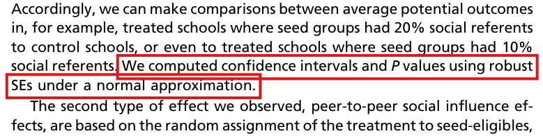
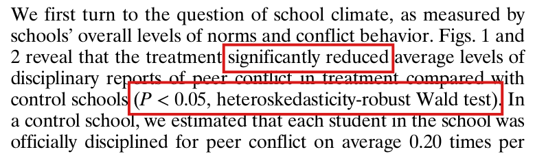
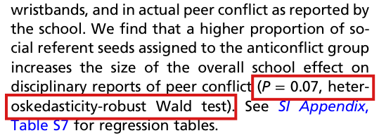
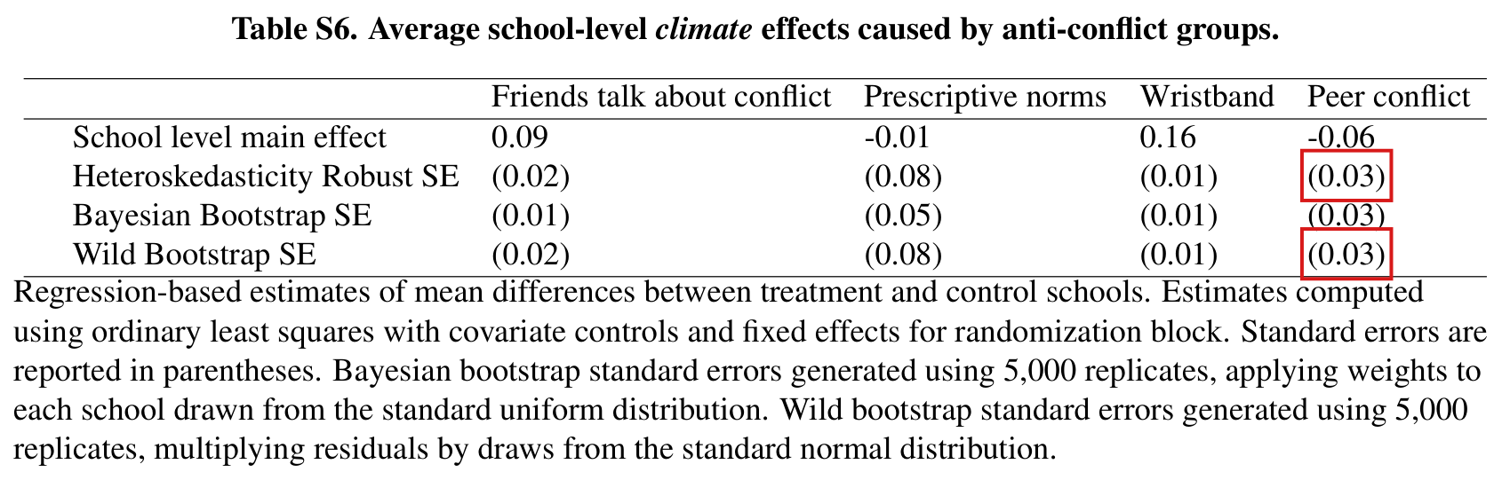
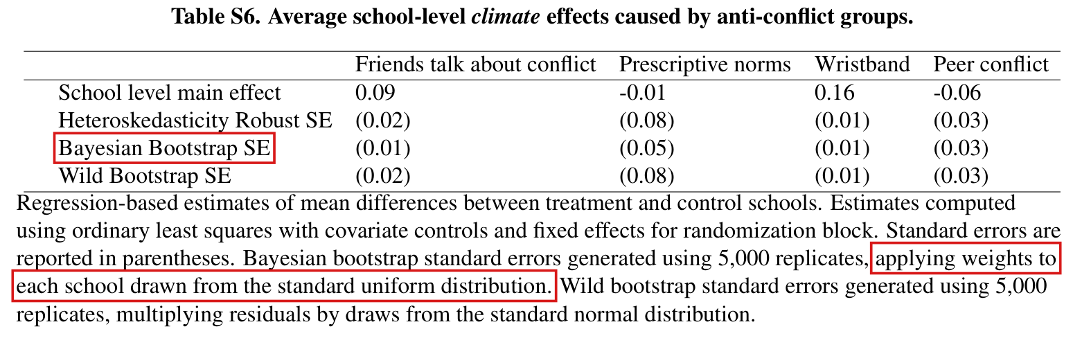
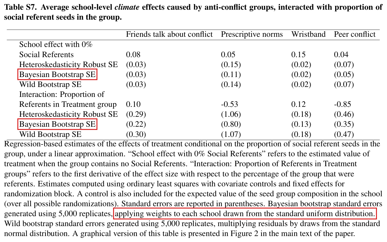
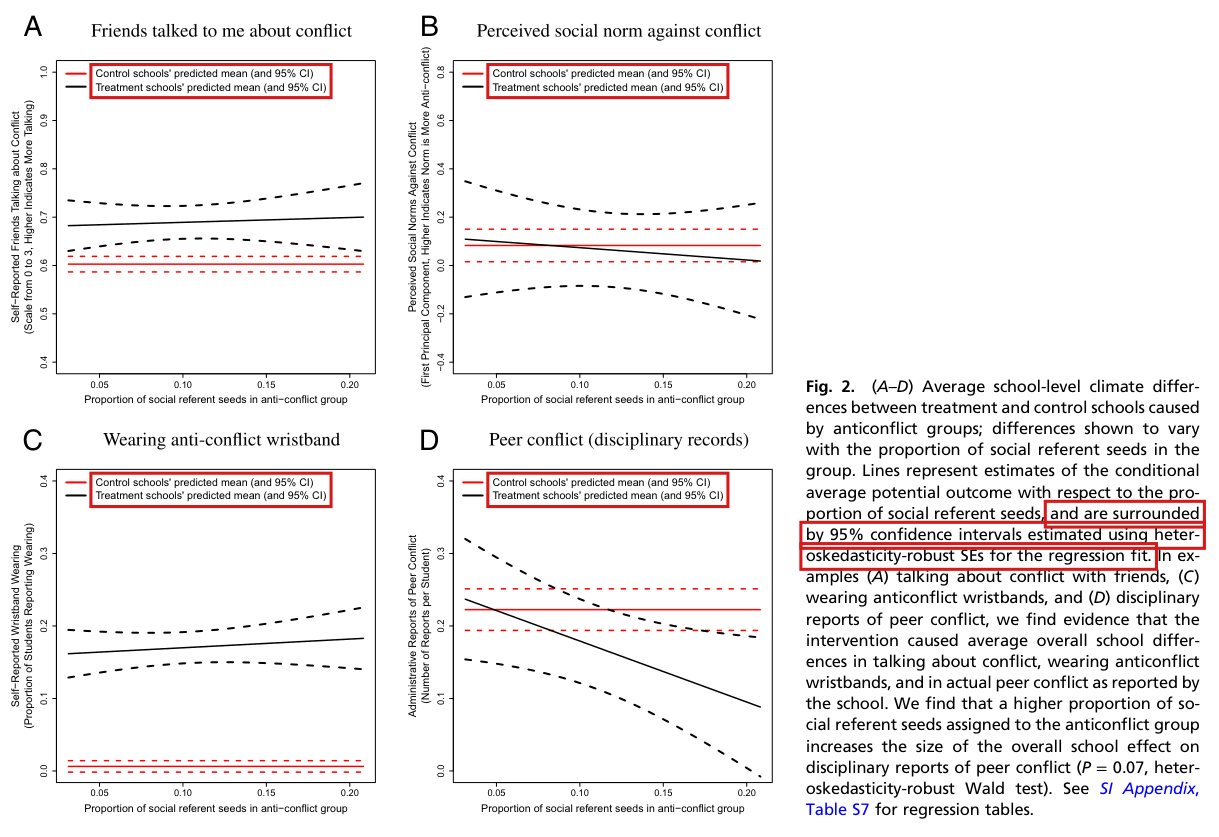
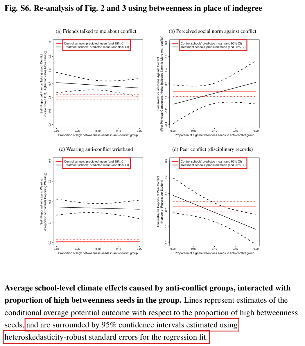
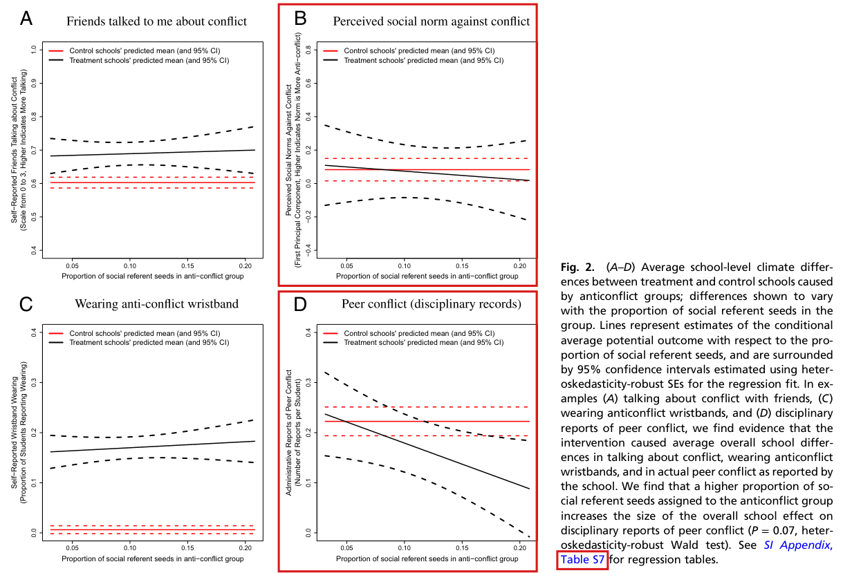
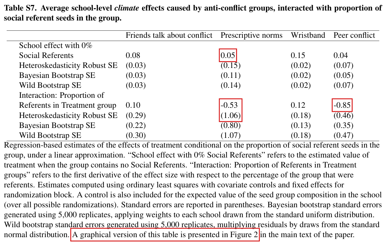
Methods and Materials, p. 568 (PDF p. 3), right column, sentence beginning “We computed confidence intervals”; Results, p. 569 (PDF p. 4), first paragraph; legend of Fig. 2, p. 569; SI Appendix, Tables S6 and S7, pp. 41–42
See also under Formal statements (Lean): P037-T18, P037-T37
I disputed this classification, but as a rule, deferred to the models’ final judgment: see my comment and the history of this entry.
As printed
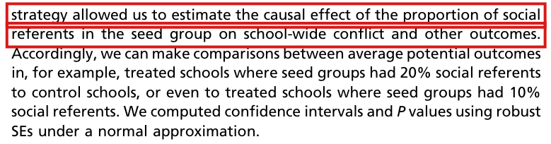
Main text, p. 568: We computed confidence intervals and values using robust SEs under a normal approximation.
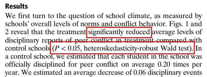
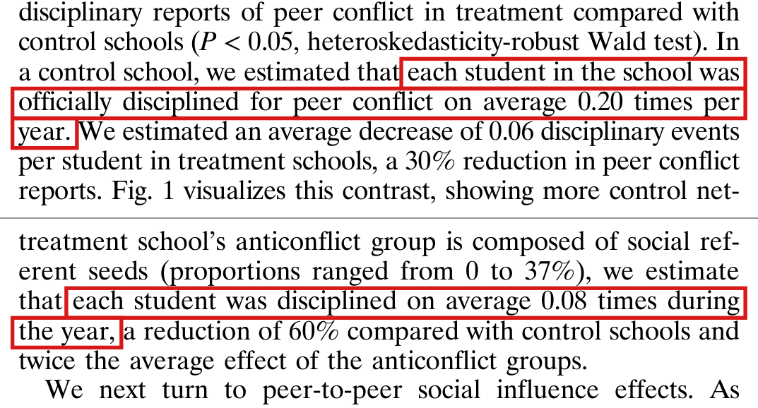
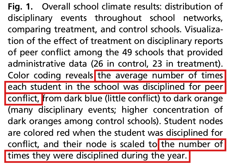
Results, p. 569: Figs. 1 and 2 reveal that the treatment significantly reduced average levels of disciplinary reports of peer conflict in treatment compared with control schools (, heteroskedasticity-robust Wald test).
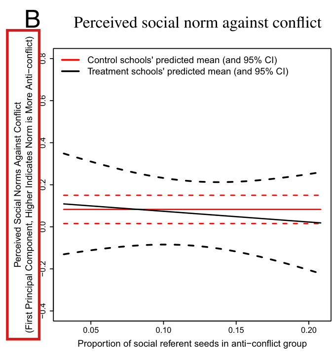
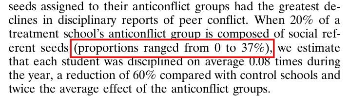
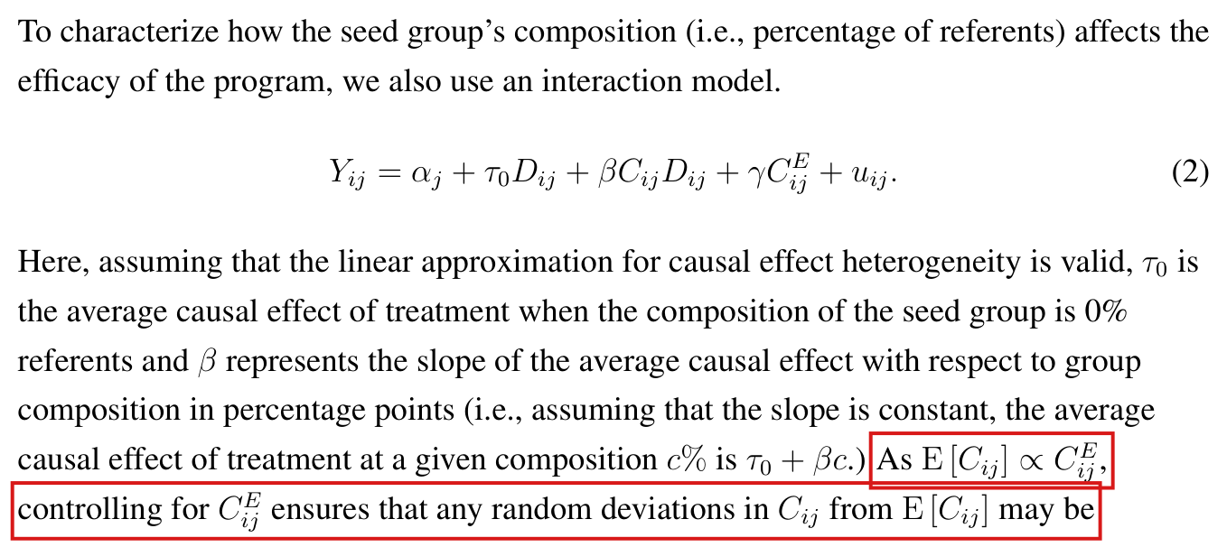
Legend of Fig. 2, p. 569: We find that a higher proportion of social referent seeds assigned to the anticonflict group increases the size of the overall school effect on disciplinary reports of peer conflict (, heteroskedasticity-robust Wald test).
Table S6 (SI p. 41), column “Peer conflict”: School level main effect ; Heteroskedasticity Robust SE ; Wild Bootstrap SE . Table S7 (SI p. 42), column “Peer conflict”, interaction: ; Heteroskedasticity Robust SE ; Wild Bootstrap SE .
The problem
The article says that the school-level confidence intervals and values use “robust SEs under a normal approximation”, and it does not name the estimator. The authors' script 4. School results-with-correction.R (lines 162–163 and 208–209) uses the heteroskedasticity-robust variance with no finite-sample adjustment, known as HC0. The wild bootstrap of Tables S6 and S7 (lines 178–195 and 228–248) multiplies the unscaled residuals by standard normal draws. Given the data, its variance is exactly HC0. The row “Wild Bootstrap SE” is therefore not a second check on the row “Heteroskedasticity Robust SE”.
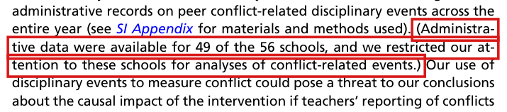
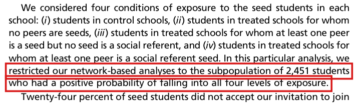
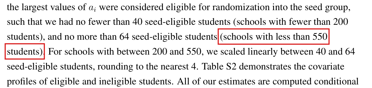
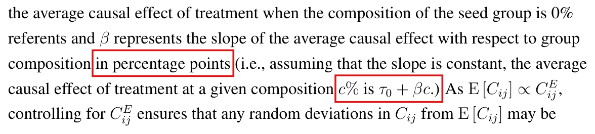
The regressions for disciplinary reports have 49 schools and many coefficients: block effects for 14 blocks, treatment, the composition terms and covariates. On the public data the regression of Table S6 has 19 estimated coefficients and that of Table S7 has 20, which leaves 30 and 29 residual degrees of freedom. Under a linear model with independent mean-zero errors of equal variance, fitting shrinks the residuals: their expected mean square is and of the error variance, whereas the expected HC0 variance is 0.62 of the variance of the treatment coefficient and 0.56 of the variance of the interaction coefficient. A normal reference does not correct for this, and the test rejects too often in the null experiments below.
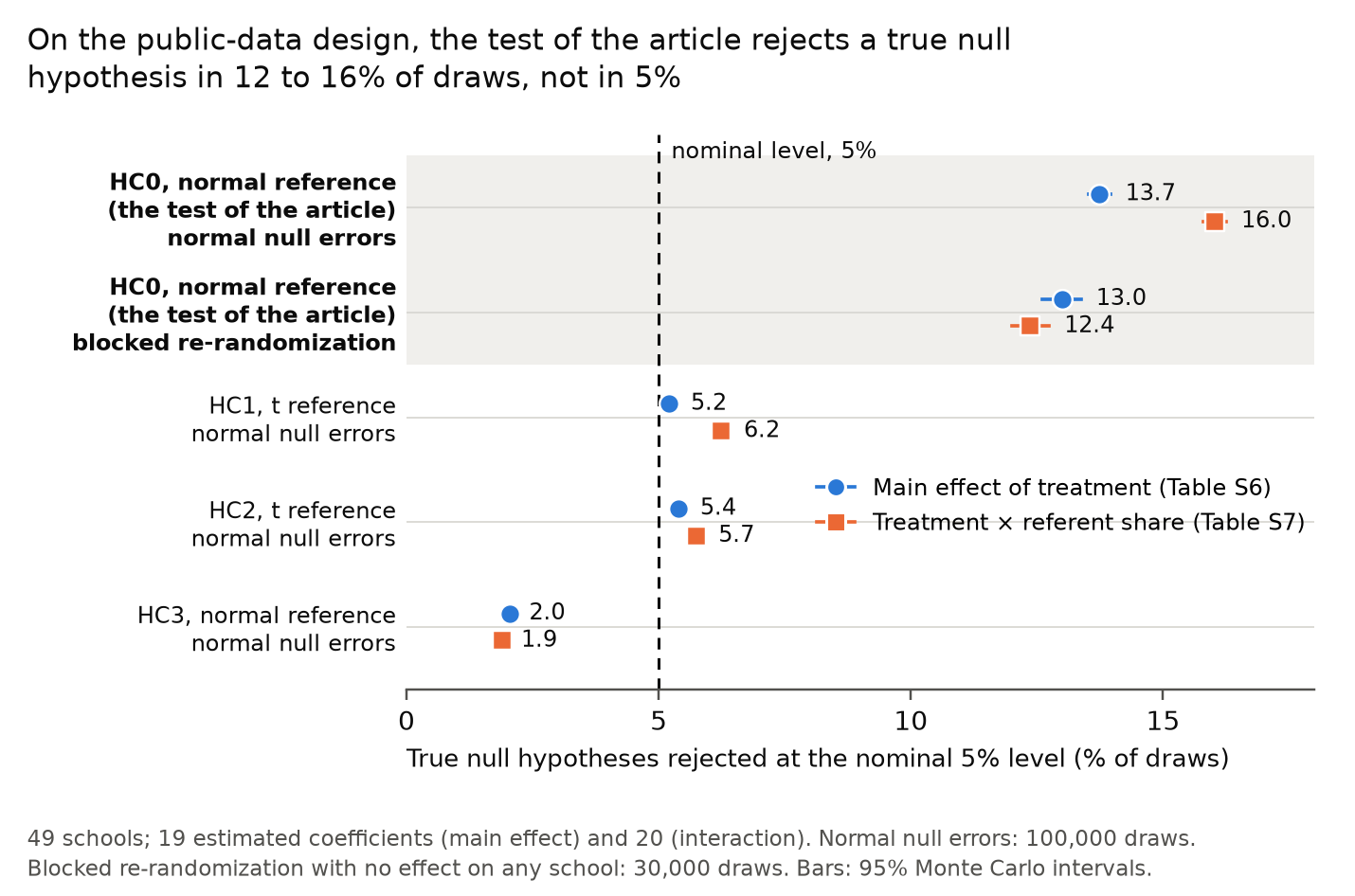
Both results on disciplinary reports rest on this test: the main effect () and the interaction with the proportion of social referent seeds (). In null experiments on the design reconstructed from the public data, the test rejects a true null hypothesis at the nominal 5% level in 12 to 16% of draws. The two printed values are weaker evidence than the same values from a calibrated test. On the public data, the test of the article gives for the main effect and for the interaction, and about and when the schools are re-randomized under the hypothesis of no effect on any school.
The description in the Methods is accurate as far as it goes, and it claims no exact size. Whether the printed values are the values of this test on the authors' own files remains unknown, because those files are not public. No replacement test is established as calibrated for the two hypotheses of the article.
Evidence a derivation
I checked the authors' script, derived the covariance identities below, calculated the estimates with the script on the public release of the data (ICPSR 37070, version 2), and examined two null experiments on the school-level design reconstructed from that release.
The bootstrap reproduces HC0. Let be the matrix of regressors, of full column rank, and write , and for the residuals. The bootstrap of the script regresses on , where the entries of are independent with mean 0 and variance 1. Its coefficient is , and hence
HC0 is too small in this design. Suppose that , where, conditional on , the errors are independent with mean zero and common variance , and let be the th diagonal entry of . Then , so
For the th coefficient, the expected HC0 variance divided by the true variance is
On the public data this ratio is for the treatment coefficient of the regression of Table S6, where the mean of is , and for the interaction coefficient of the regression of Table S7, where it is .
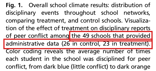
The estimates on the public data. The public-data reconstruction applies the authors' rule for selecting records, builds the network and the outcome as their scripts do, and fits their two covariate-adjusted regressions. The rule selects 49 schools, 26 control and 23 treatment, as in the article (the rule is the subject of P037-N007). The main effect is and the interaction coefficient is . The script prints estimates, standard errors and intervals, and no value; I computed each two-sided value here from the estimate and its standard error.
| Variance and reference | SE, main | , main | SE, interaction | , interaction |
|---|---|---|---|---|
| HC0, normal (the article) | ||||
| HC1, normal | ||||
| HC2, (30 and 29 d.f.) | ||||
| HC3, normal | ||||
| HC0 statistic, re-randomization |
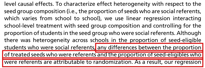
The null experiments. The first experiment draws independent standard normal errors as the outcome, 100,000 times for each of the two fixed designs, so that every coefficient is truly zero. The test of the article rejected at the nominal 5% level in 13.7% of draws for the main effect and in 16.0% for the interaction (Monte Carlo standard errors of about 0.11 percentage points). The second experiment assigns two of the four schools of each block to treatment again, 30,000 times over the 56 schools, holding the outcomes, the covariates, the draws of the seeds and the set of 49 schools fixed, as they would be if treatment had no effect on any school. The test rejected in 13.0% and 12.4% of assignments (Monte Carlo standard errors of about 0.19 percentage points). The last row of the table estimates the share of assignments in which the HC0 statistic was at least as large in absolute value as the observed one, using .
In the first experiment the variants also miss the nominal level. HC1 with a reference rejects in 5.2% and 6.2% of draws, HC2 with a reference in 5.4% and 5.7%, and HC3 with a normal reference in 2.0% and 1.9%. The experiment has normal errors of equal variance, and it does not show how these variants behave for the randomization of the study. The re-randomization calculation is for the hypothesis of no effect on any school, with the outcomes, the covariates, the draws of the seeds and the set of 49 schools held fixed. That hypothesis is stronger than a zero average effect, and stronger than a zero interaction when treatment has some effect.
What the printed tables alone allow. An effect of with HC0 standard error rounds to the entries and of Table S6. After the rescaling of the standard error by (HC1), its two-sided normal value is with coefficients and with , the two numbers of coefficients on the public data. The rescaling alone does not remove significance for every pair of values that rounds to the printed entries. With the rescaling and a reference with degrees of freedom, every such pair has ; the smallest values are and .
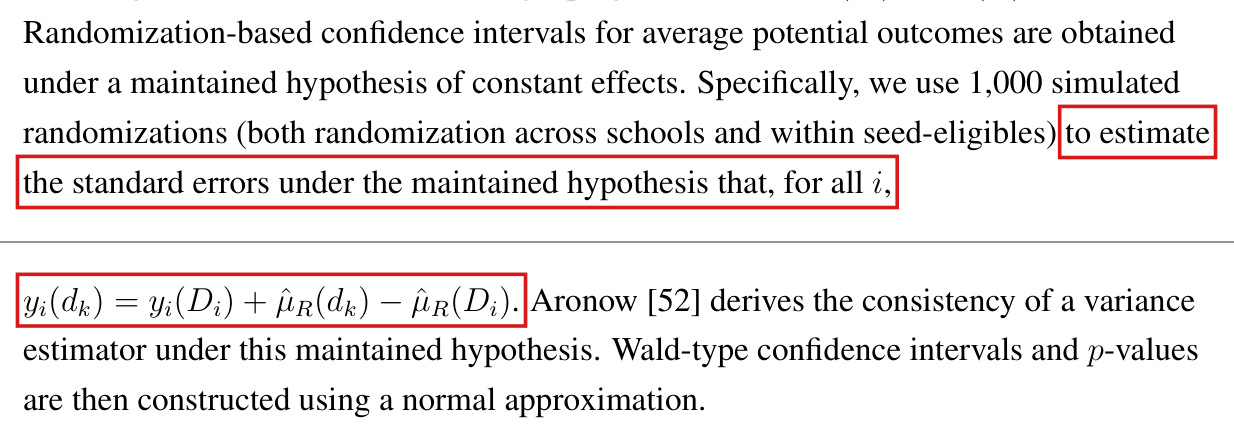
Influence-score terminology and current use. The raw empirical OLS influence covariance is exactly HC0. With schools, design row and ,
An identified current DoubleML implementation also uses an unadjusted empirical influence-score second moment: its nonclustered variance helper computes , and its official variance guide uses normal inference under regularity conditions. The sources are the captured stable guide and the pinned Python source. They establish documented continued use, without measuring its prevalence or identifying the stable documentation with a particular numeric package release. Cross-fitted DoubleML scores generally differ from these in-sample OLS residuals; their shared second-moment form transfers no finite-sample calibration to this school design.
The corrected passage below retains HC0. Reporting its public-data main-effect standard error as rather than gives an extra rounding digit; it does not provide a more accurate estimator of sampling uncertainty.
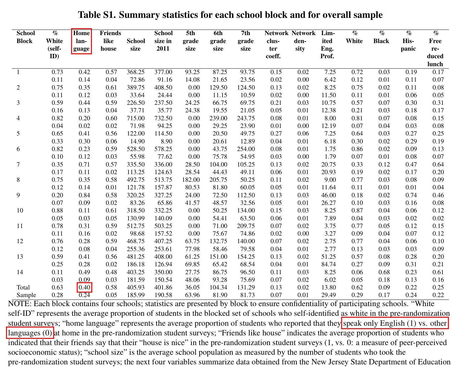
Limits. The values above are values on the public data. The authors' own input files are not public, and ICPSR states that some variables of the release were changed. On the public data the coefficient and standard error of Table S6 agree with the printed and , and the standard error and value of the interaction round to the printed and . The interaction coefficient is , which rounds to where Table S7 prints . The rejection rates are properties of the two experiments on the public-data design. They are not the rejection probability of the study under its own unknown outcomes, and the coverage of the bands of Fig. 2 was not examined.
What survives
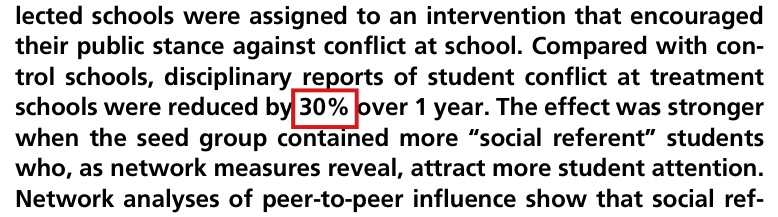
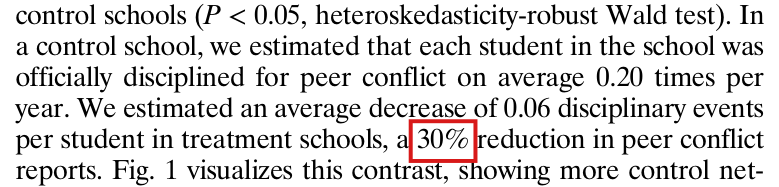
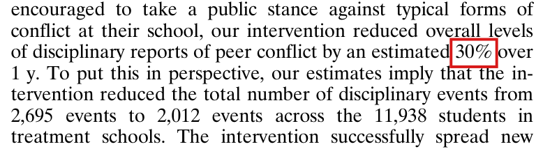
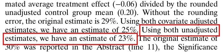
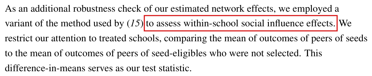
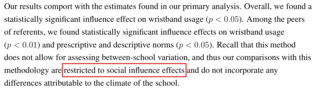
If the variance estimator or the reference distribution is changed, the least-squares estimates, their direction, the assignment of schools and the measurement of the networks do not change. The analysis of peer-to-peer influence computes its variance from simulated assignments and does not use this test. The correction of 30% to 25% is a separate matter (P037-N001).
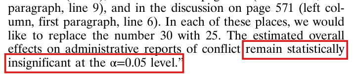
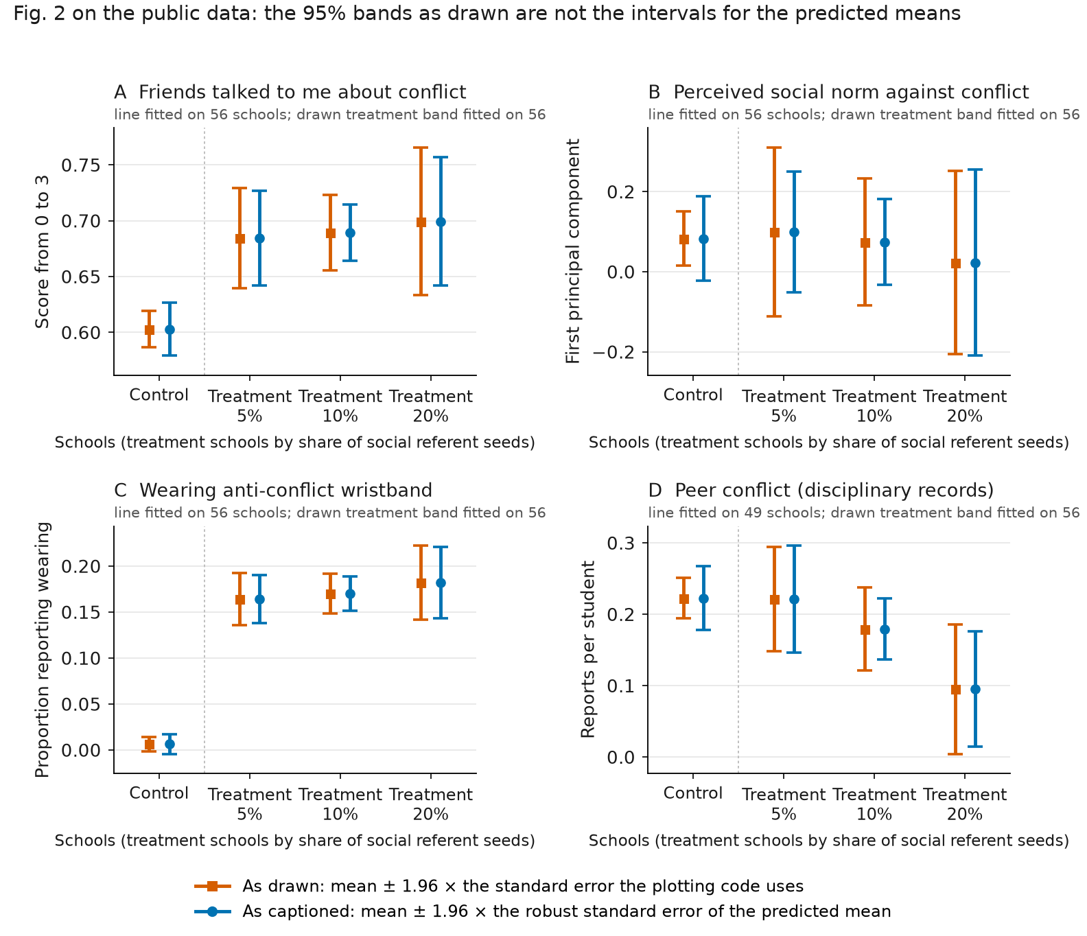
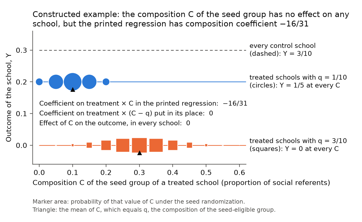
The evidence for the two results on disciplinary reports is weaker than printed. On the public data the main effect is not significant at the 0.05 level under the test of the article (), in agreement with the last sentence of the correction of 2018; the disagreement between that sentence and the article’s is the subject of P037-N008. The interaction keeps under a test that rejects a true null hypothesis in 12 to 16% of draws. The treatment bands of Fig. 2 use the same robust variance (their construction is the subject of P037-N026). No printed claim is shown to be false on the authors' own files. No test here is established as calibrated for a zero average effect and for a zero interaction in this design; the variants in the table weaken the evidence and are not such a test.
Corrected
Main text, p. 568: Confidence intervals and values use HC0 standard errors, without a finite-sample adjustment, under a normal approximation. In null experiments on the public-data design with 49 schools and 19 or 20 estimated coefficients, this test rejects a true null hypothesis more often than its nominal level.
Notes to Tables S6 and S7: The heteroskedasticity-robust standard errors are HC0. The wild bootstrap multiplies the unscaled residuals by standard normal draws. Given the data, its variance equals HC0, and it adds no finite-sample adjustment.
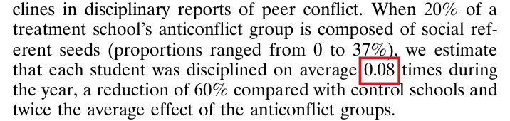
Results, p. 569: Figs. 1 and 2 show lower average levels of disciplinary reports of peer conflict in treatment compared with control schools. On the public data (ICPSR 37070, version 2) the estimate is reports per student, with HC0 standard error and two-sided under a normal reference; it is not significant at the 0.05 level.
Legend of Fig. 2, p. 569: A higher proportion of social referent seeds assigned to the anticonflict group is associated with a larger estimated overall school effect on disciplinary reports of peer conflict (on the public data, coefficient , HC0 standard error , under a normal reference).
Both values come from a test that, at the nominal 5% level, rejects a true null hypothesis in 12 to 16% of draws in null experiments on the public-data design. As sensitivity calculations on the public data, HC1 with a normal reference gives and , HC2 with a reference gives and , and a re-randomization of the schools within blocks, under the hypothesis of no effect on any school, gives and . None of these is established as a calibrated test of a zero average effect or of a zero interaction. The standard errors reported with the two estimates above remain HC0; neither the additional rounding digit nor the sensitivity calculations establish improved sampling-uncertainty estimation. The values on the authors' own files cannot be given here.












My comment and the history of this entry
Suggested classification: Moderate error.
My position My comment above; I suggested a Moderate error.
The models’ position In the independently reproduced null experiments, the HC0 inference for these 49-school fits over-rejects materially, and the proposed correction keeps the same HC0 standard errors, improving only their rounding. The central significance claim is unsupported by that procedure: Major.