P044-N005 Major
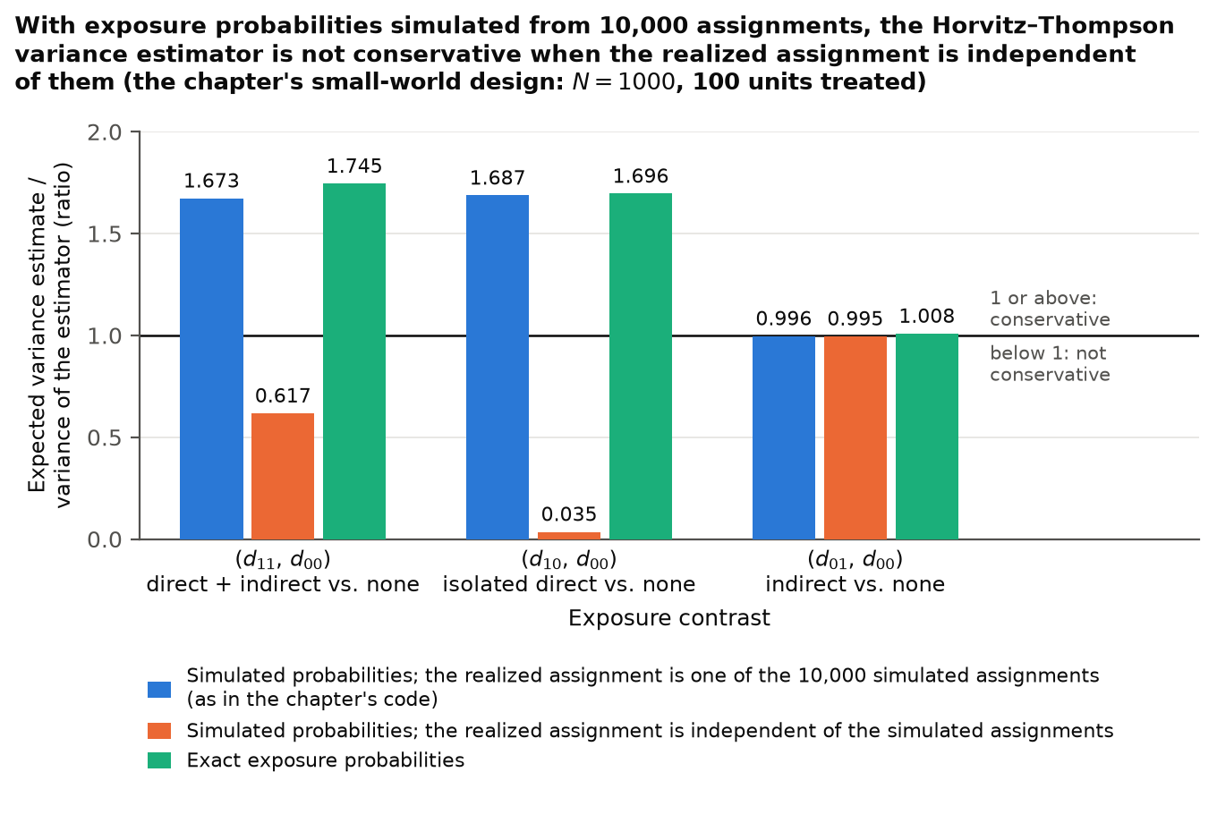
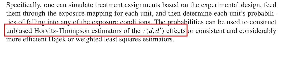
The Horvitz–Thompson variance estimator is conservative with exact exposure probabilities and positive marginal support, but not in general with probabilities simulated from 10,000 assignments, as in the chapter: in a small-world network regenerated from the printed code its expectation is 0.617, 0.035 and 0.995 times the variance of the estimator for the three contrasts when the realized assignment is independent of the simulated ones.
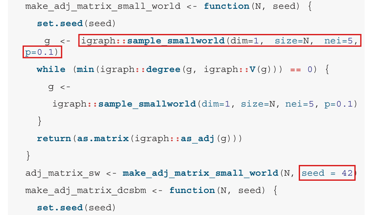
p. 217 (PDF p. 9), last paragraph, first sentence; the code lines with seed = 4224 on p. 214 (PDF p. 6) and p. 217
See also under Formal statements (Lean): P044-T1, P044-T2, P044-T11
I disputed this classification, but as a rule, deferred to the models’ final judgment: see my comment and the history of this entry.
As printed
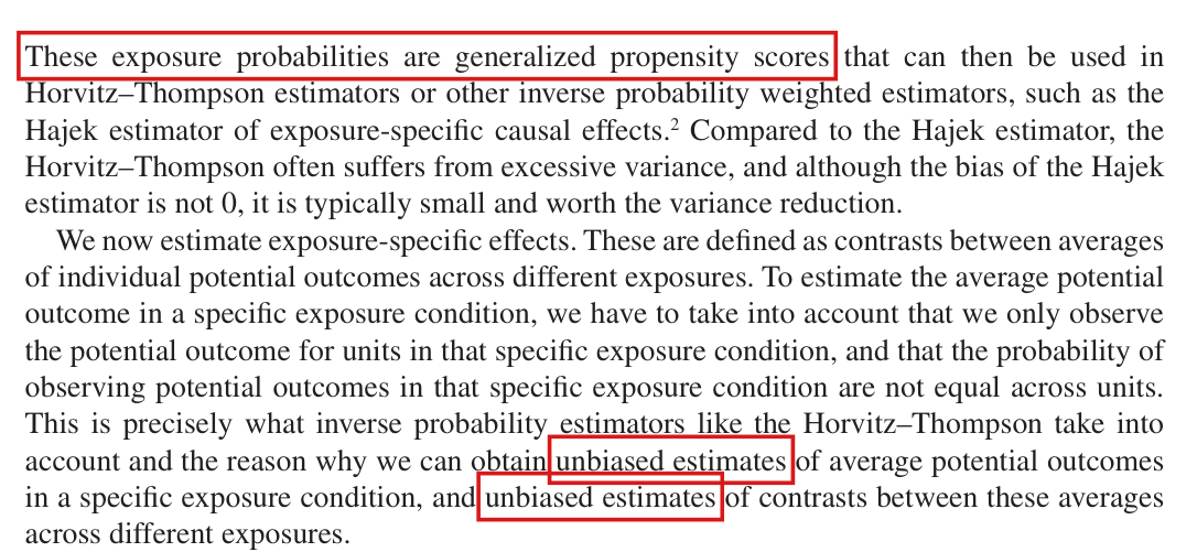
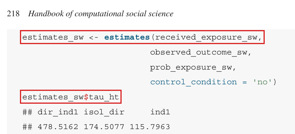
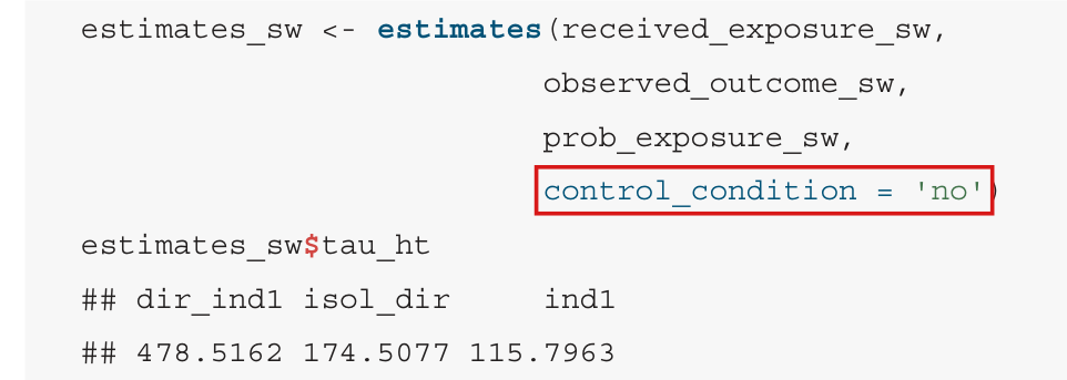
p. 217: “Next, we estimate exposure-specific effects using both the Horvitz–Thompson and Hajek estimators, as well as the variance estimators of these effects, which are conservative approximations to the exact variances.”
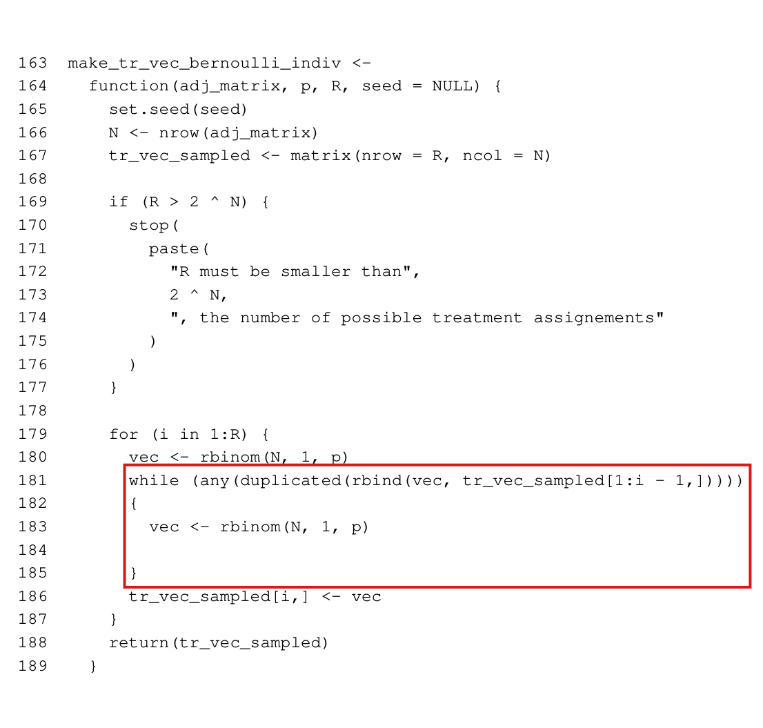
p. 214, joined on one line:
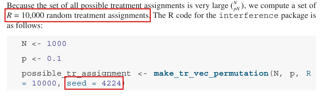
possible_tr_assignment <- make_tr_vec_permutation(N, p, R = 10000, seed = 4224)
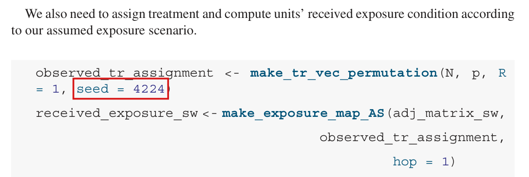
p. 217: “We also need to assign treatment and compute units' received exposure condition according to our assumed exposure scenario.”
observed_tr_assignment <- make_tr_vec_permutation(N, p, R = 1, seed = 4224)
The problem
Recall that a variance estimator is conservative if its expectation over the randomization is at least the variance of the effect estimator. The Horvitz–Thompson variance estimator has this property when it is computed with the exact exposure probabilities of the design and every unit has positive probability of both contrasted exposures. The chapter computes it with exposure probabilities simulated from assignments, and the property does not carry over. The estimator divides by the simulated probability that two units are jointly in given exposures, and for rare joint exposures this frequency rests on few assignments. In the regenerated network, among pairs of units that are both in isolated direct exposure, the smallest positive count in the 10,000 simulated assignments is 1.
Finite simulation introduces numerical error here, just as a finite number of bootstrap resamples approximates the ideal bootstrap calculation. This familiar issue can be addressed by controlling simulation error; a draw count alone does not show that the resulting Horvitz–Thompson variance estimates remain conservative.
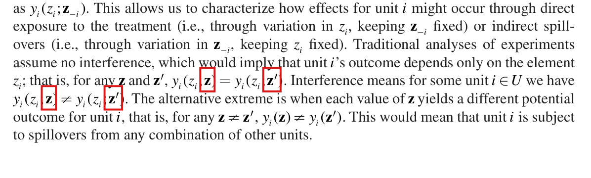
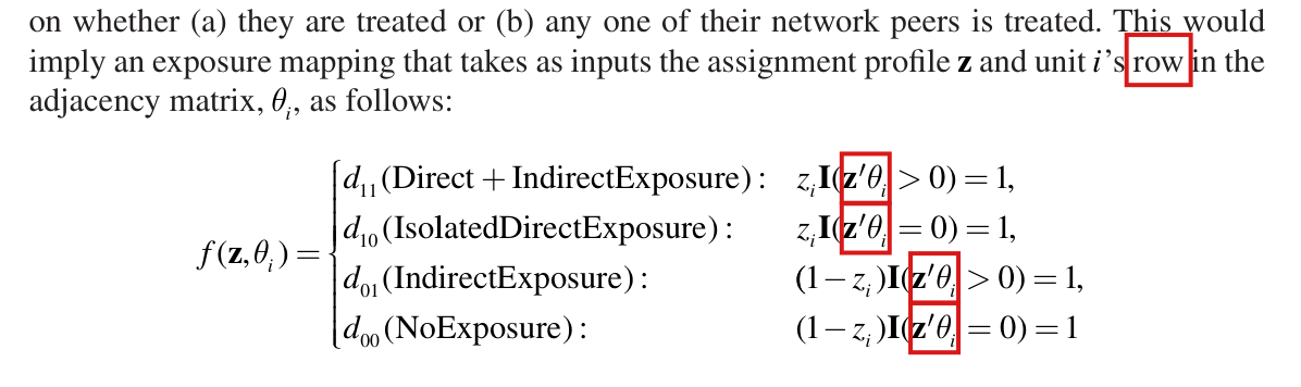
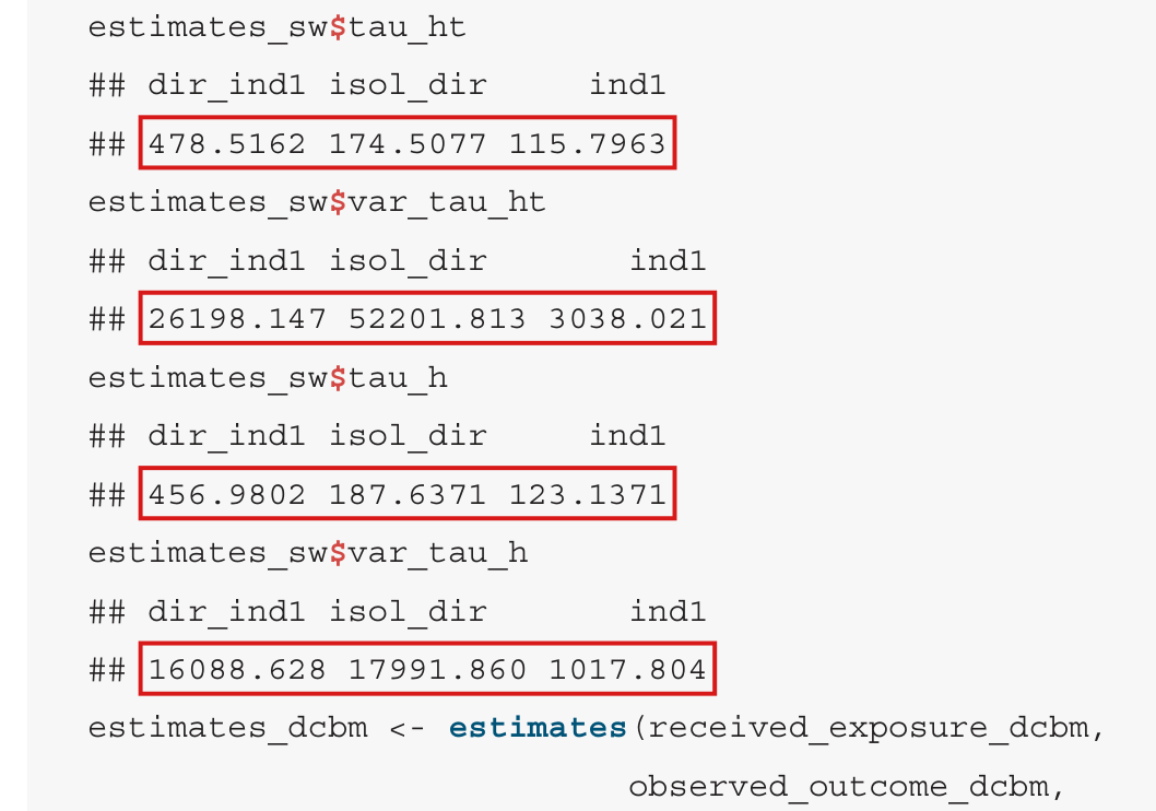
The worked example uses an assignment from the probability simulation. Both calls to make_tr_vec_permutation set the seed 4224, which implies that the realized assignment of p. 217 is the first of the 10,000 simulated assignments of p. 214. The text does not say so; it says “We also need to assign treatment”. In an experiment analyzed by this recipe, the realized assignment is ordinarily drawn independently of the simulated assignments. The two cases differ in the small-world network regenerated from the printed code. When the realized assignment is uniform among the simulated assignments, the expectation of the Horvitz–Thompson variance estimator is 1.673, 1.687 and 0.996 times the variance of the Horvitz–Thompson estimator for the contrasts , and . When the realized assignment is independent of them, the expectation is 0.617, 0.035 and 0.995 times that variance, and the observed shares of negative variance estimates are 9%, 40% and 0%. Inclusion raises the first two ratios above 1 but leaves the third below 1. Applied to an experiment, the recipe can return a Horvitz–Thompson variance estimate that is a small fraction of the variance of the estimator, or negative. Exact counterexamples show that neither a large nor a realized assignment among the simulated ones guarantees that the estimator is conservative.
Evidence an exact counterexample
I checked the claim with a recalculation in the chapter’s small-world design, exact counterexamples and a derivation, supplemented by a second recorded 10,000-assignment table and a finite-bootstrap comparison.
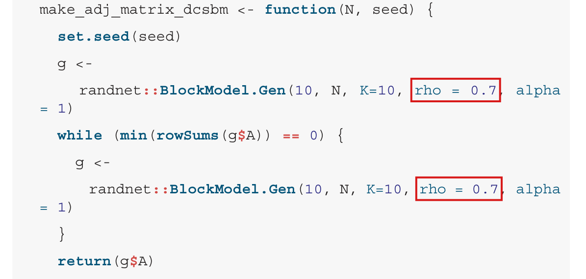
The small-world design. The small-world network was regenerated with the printed code (, nei = 5, rewiring probability 0.1, seed 42), the 10,000 simulated assignments (100 of 1000 units treated, seed 4224) and the potential outcomes (seed 547). The package then computed the exposure probabilities. The regenerated network need not be the chapter’s realization: its degree variance is 1.87 and its skewness is 0.07, against 2 and 0.12 on p. 214. Conditional on the 10,000 simulated assignments, the expectation of each variance estimator and the variance of each effect estimator were computed under two distributions of the realized assignment. In the first, the realized assignment is uniform on the 10,000 simulated assignments. In the second, it is drawn by complete randomization, independently of them. For the Horvitz–Thompson estimator, both moments are exact sums over the joint exposure probabilities of the distribution in question, with an empty exposure sum defined as zero; the package instead returns an undefined value when an exposure group is absent. The shares of negative variance estimates, the coverage and the Hajek ratios use all 10,000 simulated assignments in the first case and are estimated from 30,000 independent assignments in the second; all evaluated assignments have all four exposure groups present.
| Realized assignment | Contrast | HT ratio | HT negative | HT coverage | Hajek ratio |
|---|---|---|---|---|---|
| one of the simulated | 1.673 | 0.00% | 97.9% | 1.824 | |
| one of the simulated | 1.687 | 0.17% | 96.3% | 1.705 | |
| one of the simulated | 0.996 | 0.00% | 94.9% | 1.006 | |
| independent | 0.617 | 8.97% | 75.8% | 1.817 | |
| independent | 0.035 | 40.06% | 44.4% | 1.824 | |
| independent | 0.995 | 0.00% | 94.8% | 1.022 |
Averaging also over the simulated assignments by numerical integration, with a negligible bound on the approximation of sampling without replacement, the Horvitz–Thompson ratios are 1.664, 1.667 and 0.996 in the first case and 0.632, 0.072 and 0.980 in the second. With exact exposure probabilities the ratios are 1.745, 1.696 and 1.008. With exact marginal probabilities and simulated joint probabilities they are 0.648, 0.020 and 1.006 for an independent realized assignment. This shows that the shortfall persists with exact marginal probabilities. The ratios for the degree-corrected block model were not computed.
Exact counterexamples. In each, the exposure mapping is the chapter’s, treatment is by complete randomization, and every unit has positive probability of each of the four exposures. The contrast is . The simulated assignments are a uniform sample of distinct assignments, as make_tr_vec_permutation draws them, and the moments are exact rational numbers.
- Twelve units form three disjoint cliques of four, two units are treated, all potential outcomes equal 1, and the probabilities are simulated from 65 of the 66 assignments. Over all such samples, the variance of the Horvitz–Thompson estimator is 0.48766 and the expected variance estimate is 0.44710 when the realized assignment is independent of the sample. They are 0.48734 and 0.44874 when it is one of the 65. With exact probabilities both equal .
- Ten units form a cycle, two units are treated, and the other potential outcomes are 0, and the probabilities are simulated from 20 of the 45 assignments. Over all such samples, the expected variance estimate is against a variance of 0.0370 when the realized assignment is independent of the sample, and 0.0173 against 0.0334 when it is one of the 20. With exact probabilities the expected variance estimate is and the variance is .
- Forty units form eight disjoint cliques of five, four units are treated, all potential outcomes equal 1, and the probabilities are simulated from one recorded sample of of the 91,390 assignments. Given this sample, the expected variance estimate is 0.12980 against a variance of 0.13262 when the realized assignment is independent of the sample, and 0.13013 against 0.13036 when it is one of the 10,000.
For a second probability table for the same forty-unit design, using Python seed 20261019 for its 10,000 distinct assignments, I obtain an expected variance estimate of against variance for an independent realized assignment, and against when the realized assignment is included. Every positive relevant joint has a positive empirical count, with minimum 845; exact probabilities give equality at . These moments condition on this probability table rather than averaging over all 10,000-assignment samples. Both tables concern this forty-unit design rather than the chapter’s published networks, and neither calculation establishes a numerical error in a published table entry.
Finite simulation and accuracy. The literal bootstrap analogy concerns a computational approximation. For fixed observed data , the ideal variance of a two-observation bootstrap mean is . With independent bootstrap means, their sample variance with denominator has expectation , but is zero with probability ; denominator gives expectation . This illustrates finite computational error without equating its bias mechanism to the nonlinear Horvitz–Thompson plug-in or establishing bootstrap validity for an original sampling distribution.
The package samples distinct assignments by default. If assignments are possible and an exposure event has exact probability , its count in uniform draws without replacement is hypergeometric, with
Thus its relative standard deviation depends on , not on alone. At and negligible sampling fraction, the illustrative probabilities , and give relative standard deviations about , and ; these are not measurements of the chapter’s graph. The routine also uses for marginals, for same-exposure off-diagonal joints and for cross-exposure joints. Smoothing and these distinct normalizers must be included in an accuracy argument, along with support and zero-count handling. A bound holding with high probability does not alone prove conservative expectation without control of the failure event and any needed margin or inflation.
For independent with-replacement simulation from a fixed finite design, fixed finite outcomes and mapping, positive contrast marginals and finitely many relevant positive joints, the strong law and vanishing smoothing give almost-sure convergence of the coefficient formulas and their fixed-design conditional moments to their exact-probability counterparts once support is correctly distinguished. This is no finite- inequality, no uniform guarantee over changing designs or shrinking positive joints, no growing- result, and no coverage guarantee. For the default without-replacement scheme, at fixed design; even a full census retains the routine’s smoothing. Analytic probabilities or unsmoothed census frequencies are exact alternatives. Sufficiently accurate simulation with justified error accounting can also be adequate.
Derivation for exact probabilities. Let and , with , and write and . The Horvitz–Thompson estimator of the total under is , and . The variance estimator is , where
Each term of the two sums over positive joint probabilities has expectation equal to the corresponding term of or of . For a pair with , the term of the variance is , and the second sum of has expectation for that pair. For a pair with , the term of the covariance is , and the second sum of has expectation . Collecting terms gives
The first step of this computation uses that the probabilities inside are those of the distribution of the realized assignment. With simulated probabilities in their place the identity fails, as the counterexamples show.
What survives
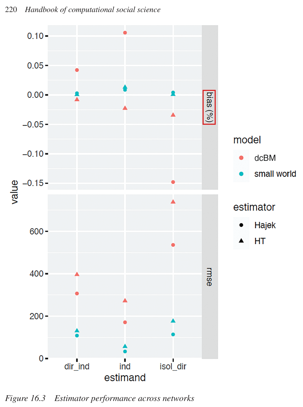
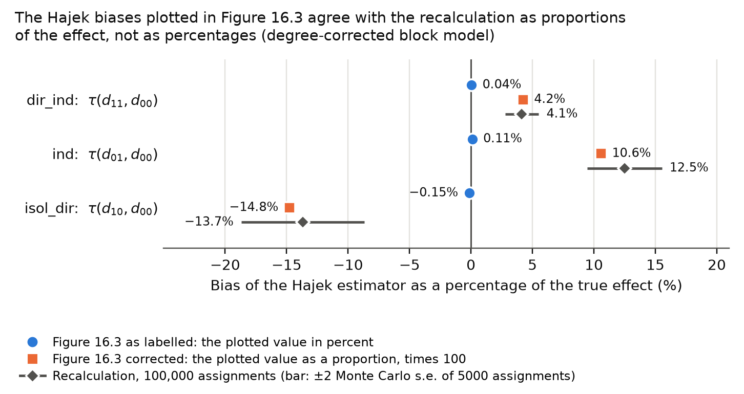
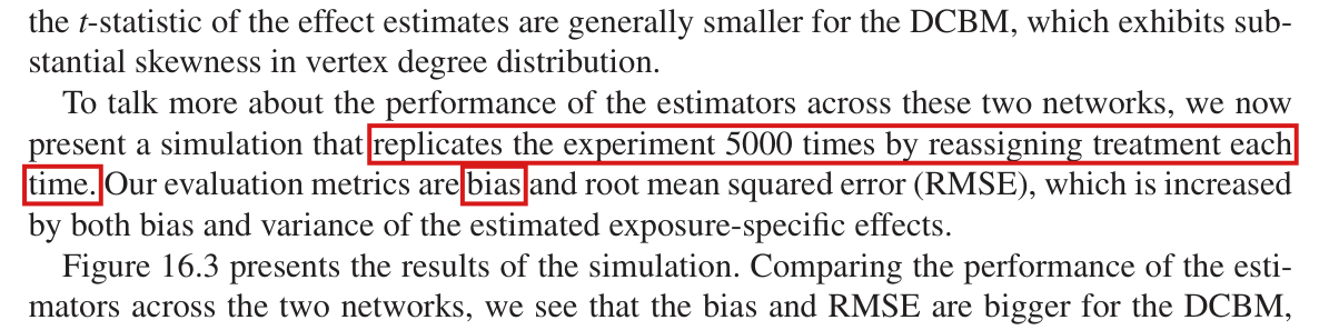
The exposure mapping, the estimands and the Horvitz–Thompson variance estimator computed with exact exposure probabilities under positive marginal support are unaffected. No entry of Table 16.1 is shown to be wrong. Its Horvitz–Thompson standard errors and -statistics were computed with the realized assignment among the simulated assignments, and they describe that case. Figure 16.3 reports the bias and the RMSE of the point estimators and does not depend on the variance estimators. In the regenerated small-world design, the Hajek variance ratios are approximately between 1.01 and 1.82 in the first case and are estimated to lie approximately between 1.02 and 1.82 in the independent case. These results concern that design and give no general guarantee. What is lost is the assurance that the Horvitz–Thompson variance estimator computed with simulated exposure probabilities is conservative.
Corrected
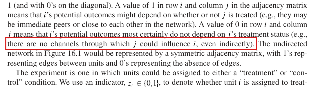
Next, the exposure-specific effects are estimated using both the Horvitz–Thompson and Hajek estimators, together with variance estimators of these effects. Let and be the exact exposure probabilities of the design, and suppose that and for every unit . Then the Horvitz–Thompson variance estimator computed with these probabilities, including its terms for pairs of units with joint exposure probability zero, is conservative:
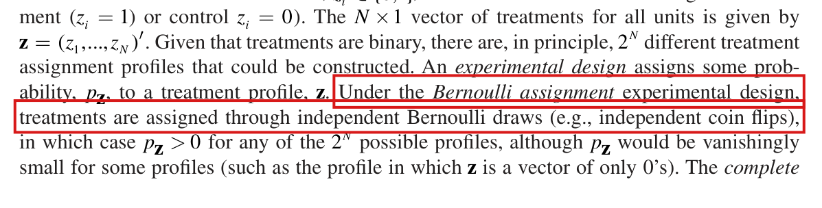
The exposure probabilities used below are simulated from assignments, and the variance estimator computed from them need not be conservative, even at and even if the realized assignment is one of the simulated assignments, as it is in the code below, where both calls use seed 4224. Exact probabilities retain this variance guarantee; a method using simulated probabilities needs a separate justification that accounts for their simulation error. Increasing the number of assignments with suitable accuracy checks is one possible computational remedy; the necessary effort depends on the joint exposure probabilities relevant to the contrasts. This expectation guarantee alone does not guarantee confidence-interval coverage. The Hajek variance estimator is a linearized approximation and has no general finite-sample guarantee.
For the design of the examples the exact probabilities have closed forms. Under complete randomization of of units, the probability that given units are treated and other given units are not is . For a unit with neighbors, , , and . The joint probabilities follow in the same way by inclusion and exclusion over the two neighbor sets.










My comment and the history of this entry
Suggested classification: Moderate error.
My position My comment above; I suggested a Moderate error.
The models’ position The Horvitz–Thompson variance estimator is conservative with exact exposure probabilities and positive marginal support. In a small-world network regenerated from the chapter’s printed code, the finite simulation recipe can severely understate variance when the realized assignment is independent of the simulated assignments, which undermines a central guarantee of conservativeness: Major. No published table entry is shown to be wrong.