LLM-generated corrections to the published research of P. M. Aronow

Book chapter P045

Corrections to: Spillover Effects in Experimental Data

P. M. Aronow, Dean Eckles, Cyrus Samii, and Stephanie Zonszein (2021). Spillover Effects in Experimental Data. In Advances in Experimental Political Science.

DOI
10.1017/9781108777919.021
arXiv
2001.05444
Audited edition
Advances in Experimental Political Science, 2021; 31 pages in the audited file
SHA-256 of the audited file
0db5a6f02a106e561bd0aa527292dafd2f6f9852abb2374c959a64d40bcde5df
Permanent address
https://pmaronow.github.io/llm-audit/works/P045/

Summary

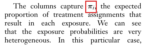
This chapter reviews methods for estimating direct and spillover effects in randomized experiments under interference. It covers exposure mappings with Horvitz–Thompson and Hajek estimators on a known network, the Hudgens–Halloran estimators under partial interference, and the relation between interference and contagion, and it illustrates them with the interference R package. 15 entries are classified as errors (5 Moderate, 10 Minor), and 9 are clarity notes; 5 further concerns were not confirmed, 3 remain unresolved and 4 fall outside the scope of this chapter. With Bernoulli assignment inside groups, the within-arm sample means of Section 16.5.1 are not generally unbiased under interference (P045-E001). I clarify the distinction between the exact-probability variance guarantee and its intended Monte Carlo approximation (P045-N016).

What was and was not checked

I read all 31 pages of the chapter, with every display, table, figure, footnote and reference, together with the source code of two versions of the interference package. The following points were checked and held up.

  • The example with ten units (pp. 295–298). The printed adjacency matrix agrees with Figure 16.3 edge by edge. Taking that matrix as input and using the sampling algorithm that was the default before R 3.6.0, I reproduced the treatment assignment, the exposure matrix, the printed exposure probabilities and the contrasts 41.6104341.61043 and 39.5164339.51643 from the package code. The remaining entry of that output is the subject of P045-E004, and the form of the printed probabilities is the subject of P045-N001.
  • The Horvitz–Thompson estimator of p. 297 is exactly unbiased over the 45 assignments of that example when the exact exposure probabilities are used.
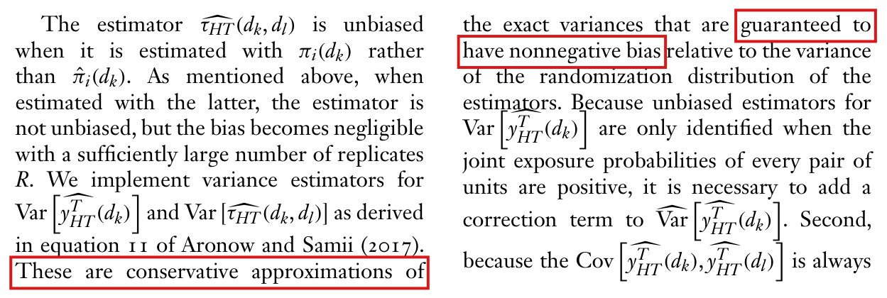
  • The variance code of the package implements the variance and covariance expressions described on pp. 298–299. For the Horvitz–Thompson estimators, the nonnegative-bias guarantee holds with exact marginal and joint exposure probabilities; finite Monte Carlo substitution need not preserve that exact guarantee (P045-N016).
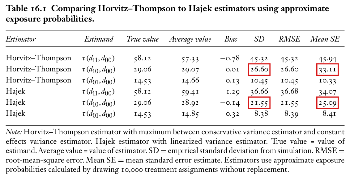
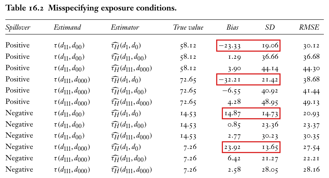
  • Tables 16.1, 16.2 and 16.3. In every row of the three tables the RMSE equals Bias2+(2999/3000)SD2\sqrt{\text{Bias}^2+(2999/3000)\text{SD}^2} up to rounding, with SD interpreted as a sample standard deviation over 3000 replications, and in every row of Tables 16.1 and 16.3 the bias equals the average value minus the true value. The true values of Tables 16.1 and 16.2 are in the ratios that the multipliers imply. In Table 16.1 the Hajek estimator has the smaller SD and RMSE in every comparison, and in Table 16.2 the biases have the signs that the text states.
  • Figure 16.4 agrees with Table 16.2 in all twelve panels: the dashed lines agree with the tabulated true values within 0.10.1, the means estimated from the histogram bins minus the dashed lines agree with the tabulated biases within 0.450.45, and the standard deviations estimated from those bins agree with the tabulated SDs within 0.70.7.
  • The example with eighteen units (p. 311). The package reproduces all five point estimates and all five variances on a reconstructed dataset compatible with the six printed rows and every reported digit; this does not identify the original dataset or seed. The identities between the total, direct, indirect and overall estimates hold within rounding. Under the two-stage complete randomization of that example and stratified interference, the five point estimators are exactly unbiased over its 14,580 assignments. P045-N008 concerns the two direct-effect variances.
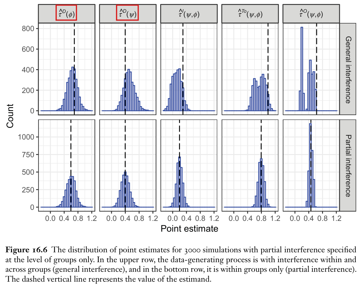
  • Figure 16.6. After swapping the first two column labels (P045-E014) and using a common baseline mean inferred from the figure, the dashed lines agree with the estimands implied by the multipliers of the package to plotting precision, and the means estimated from the histogram bins agree with the expectations of the estimators derived from them within 0.0030.003.
  • The decomposition θ=γ(1)+η(0)=γ(0)+η(1)\theta=\gamma(1)+\eta(0)=\gamma(0)+\eta(1) on p. 315 follows from the printed definitions.
  • The arithmetic in the summaries of the empirical studies (Figure 16.2 and the experiment of Nickerson) agrees with the reported figures up to rounding.

I did not have the scripts, seeds and draws behind Tables 16.1–16.3 and Figures 16.4–16.6, so I could not recompute those results from their source. I checked them by arithmetic, by reading the figures and by independent simulations on new network draws. These simulations reproduce the ordering of the estimators in Table 16.1 with similar magnitudes, give biases close to the printed ones in the cases of Table 16.2 that were simulated, and reproduce the ranking of designs and estimators in Table 16.3. They do not reproduce the magnitudes of Table 16.3: the simulated standard deviations are smaller and the biases differ, and without the script behind that table the difference could not be resolved. The works that the chapter cites and the empirical studies that it summarizes were consulted only on a few specific points. Otherwise, only the internal consistency of what the chapter reports about them was checked. I also examined the chapter’s description of the experiment of Paluck, Shepherd and Aronow (2016); P045-N018 clarifies the wording on p. 307. The chapter accurately attributes the school-composition finding to that study, with its causal interpretation conditional on the study’s response model; no correction of that attribution is established.

No appendix or supplement to the chapter was identified. The replication script distributed with the package reproduces a table of Aronow and Samii (2017) and not the results of this chapter. These checks cover the points listed above. They do not establish that the rest of the chapter is correct.

The context of the variance discussion on pp. 294 and 298–299 naturally distinguishes an exact-probability theorem from accurate Monte Carlo approximation (P045-N016). The finite-draw counterexample shows that Monte Carlo substitution need not preserve the exact sign guarantee; it does not establish an error in the chapter’s 10,000-draw calculations, its maximum variance estimator or a published simulation value, nor a confidence-interval coverage failure.

Headline claims and related corrections

  1. With a known interference network and a correctly specified exposure mapping, exposure probabilities follow from the design, and exposure-specific average potential outcomes and their contrasts are estimated without bias by Horvitz-Thompson weighting (Aronow and Samii 2017); the interference R package carries this out in a 10-unit toy example.

    Sections 16.4.1-16.4.2; exposure-mapping and HT displays on pp. 294 and 297; Figure 16.3; toy example code and output on pp. 295-298

    See P045-E004, P045-E007, P045-E008, P045-A001, P045-N001.

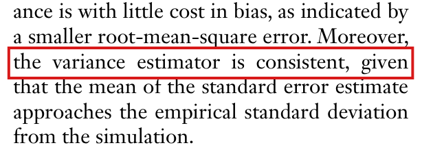
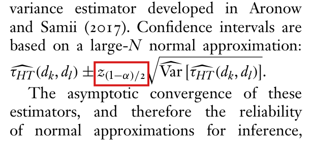
  2. In a 400-unit small-world simulation the Hajek estimator is more efficient than Horvitz-Thompson at little cost in bias (smaller RMSE), and the chapter states that the variance estimator is consistent because the mean standard error approaches the empirical standard deviation.

    Section 16.4.2, p. 299; Table 16.1; Hajek display

    See P045-N002, P045-E005.

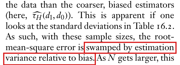
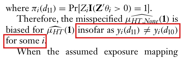
  3. If the assumed exposure mapping is coarser than the true interference, estimators of the all-versus-none effect τ(1,0)\tau(\mathbf{1},\mathbf{0}) are biased (downward under positive spillover, upward under negative spillover); if it is as fine or finer, they are centred on the truth but more variable.

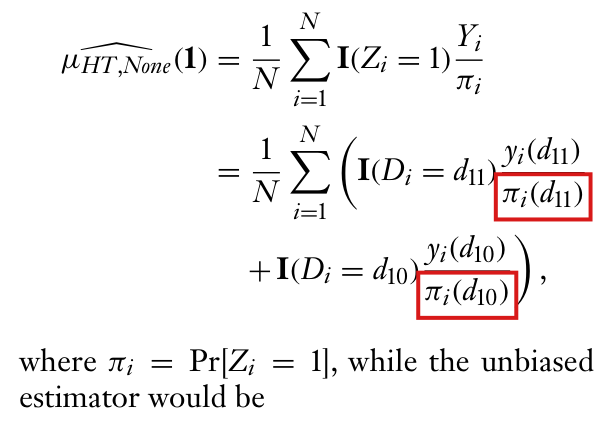
    Section 16.4.3, pp. 299–303; Table 16.2; Figure 16.4; the μ^HT,None(1)\widehat{\mu}_{HT,\mathrm{None}}(\mathbf{1}) display on p. 301; Proposition 8.1 of Aronow and Samii (2017)

    See P045-E002, P045-E005, P045-E015, P045-E016.

  4. When the measured network is missing ties, the estimators are biased and the bias grows with the proportion of missing ties; the distributions are centred at 0% missing and shift as the proportion rises.

    Section 16.4.4, p. 303; Figure 16.5

    See P045-E012.

  5. For the full-neighbourhood contrast, graph cluster randomization (3-net clustering) gives substantially lower estimator variability (lower SD and RMSE) than unit-level Bernoulli(1/2)(1/2) randomization, at no cost in bias.

    Section 16.4.6, pp. 304-306; Table 16.3; full-neighbourhood exposure mapping

    See P045-E011, P045-E010, P045-E013, P045-E006.

  6. Under partial interference and a two-stage randomized saturation design, the chapter states that the Hudgens–Halloran arm means and direct, indirect, total and overall effect estimators are unbiased conditional on their denominators being nonzero, without knowledge of the within-group network. It states that the variance estimators under stratified interference are unbiased with additive effects and conservative otherwise; the package function estimates_hierarchical computes them in an 18-unit example.

    Section 16.5.1, pp. 308-311; marginal-effect and estimator displays on pp. 309-310; toy output on p. 311

    See P045-E001, P045-E009, P045-N008.

  7. If interference also runs across groups within tracts while the analyst assumes partial interference at the group level, the direct, indirect, total and overall estimators are biased; they are unbiased when partial interference holds.

    Section 16.5.2, pp. 311–312; Figure 16.6; the y^(z;ψ)\widehat{y}(z;\psi) mixture display on p. 312

    See P045-E003, P045-E014.

  8. Contagion is one (outcome-mediated) mechanism of interference; the indirect effect decomposes into a contagion effect and other mechanisms, θ=γ(1)+η(0)=γ(0)+η(1)\theta=\gamma(1)+\eta(0)=\gamma(0)+\eta(1), and identifying the decomposition needs mediation assumptions (sequential ignorability, a cross-world assumption) beyond randomized treatment assignment.

    Figure 16.1; Section 16.6, pp. 314–316; displays for θ\theta, γ(z)\gamma(z) and η(z)\eta(z) on p. 315

  9. The reviewed empirical studies show that spillovers matter (voting, petitioning, student behaviour, prejudice, economic outcomes), that inter-group comparisons can conceal within-group spillovers and that effects depend on the assignment regime, and they illustrate designs that implement the two frameworks.

    Figure 16.2; Sections 16.2, 16.4.7, 16.5.3; conclusion p. 316

    See P045-N009, P045-N010.

Corrections

Moderate (5)

A real substantive error with limited reach.

Under Bernoulli assignment within groups, the arm means of Section 16.5.1 are not in general unbiased for the marginal potential outcomes of p. 309, and neither are the estimators of the direct, indirect and total effects built from them; the estimator of the overall effect is unbiased under uniform assignment of fixed positive numbers of groups to saturations.

Section 16.5.1, p. 310 (PDF p. 22), left column, the paragraph beginning “Let the observed outcome be” and its two displays

See also under Formal statements (Lean): P045-T1, P045-T2, P045-T25

As printed

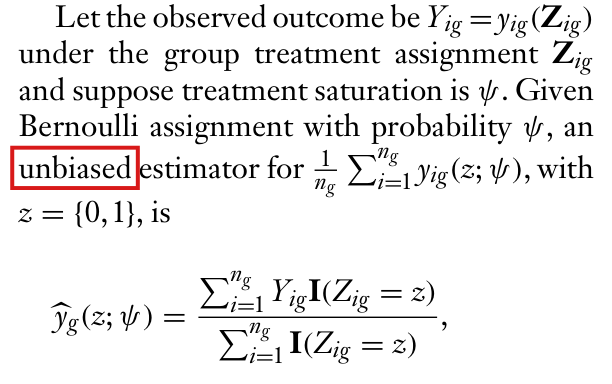
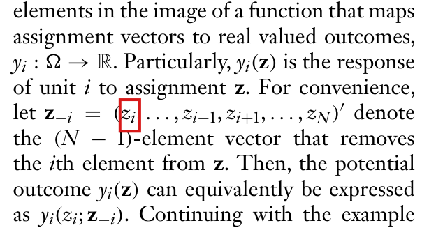
Let the observed outcome be Yig=yig(Zig)Y_{ig}=y_{ig}(\mathbf{Z}_{ig}) under the group treatment assignment Zig\mathbf{Z}_{ig} and suppose treatment saturation is ψ\psi. Given Bernoulli assignment with probability ψ\psi, an unbiased estimator for 1ng∑i=1ngyig(z;ψ)\frac{1}{n_g}\sum_{i=1}^{n_g}y_{ig}(z;\psi), with z={0,1}z=\{0,1\}, is

y^g(z;ψ)=∑i=1ngYigI(Zig=z)∑i=1ngI(Zig=z),\widehat{y}_g(z;\psi)=\frac{\sum_{i=1}^{n_g}Y_{ig}\mathbf{I}(Z_{ig}=z)}{\sum_{i=1}^{n_g}\mathbf{I}(Z_{ig}=z)},

and for the population average potential outcome, it is

y^(z;ψ)=∑g=1Gy^g(z;ψ)I(Sg=ψ)∑g=1GI(Sg=ψ),\widehat{y}(z;\psi)=\frac{\sum_{g=1}^{G}\widehat{y}_g(z;\psi)\mathbf{I}(S_g=\psi)}{\sum_{g=1}^{G}\mathbf{I}(S_g=\psi)},

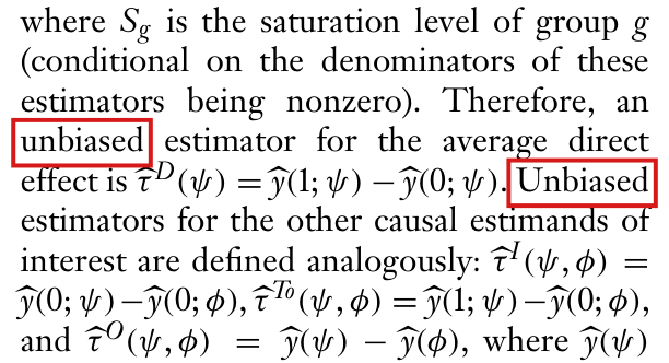
where SgS_g is the saturation level of group gg (conditional on the denominators of these estimators being nonzero). Therefore, an unbiased estimator for the average direct effect is τ^D(ψ)=y^(1;ψ)−y^(0;ψ)\widehat{\tau}^{D}(\psi)=\widehat{y}(1;\psi)-\widehat{y}(0;\psi). Unbiased estimators for the other causal estimands of interest are defined analogously: τ^I(ψ,ϕ)=y^(0;ψ)−y^(0;ϕ)\widehat{\tau}^{I}(\psi,\phi)=\widehat{y}(0;\psi)-\widehat{y}(0;\phi), τ^To(ψ,ϕ)=y^(1;ψ)−y^(0;ϕ)\widehat{\tau}^{To}(\psi,\phi)=\widehat{y}(1;\psi)-\widehat{y}(0;\phi), and τ^O(ψ,ϕ)=y^(ψ)−y^(ϕ)\widehat{\tau}^{O}(\psi,\phi)=\widehat{y}(\psi)-\widehat{y}(\phi), where y^(ψ)\widehat{y}(\psi) is the average across groups assigned to saturation ψ\psi of the average observed outcomes of units in the group under treatment assignment Zig\mathbf{Z}_{ig}.

The problem

On p. 309 the chapter defines the marginal potential outcome yig(z;ψ)y_{ig}(z;\psi) by fixing the treatment of unit ii at zz and averaging its potential outcomes over the treatments of the other group members, each of whom is treated independently with probability ψ\psi. The same page separates this from complete random assignment, which fixes the number of treated units. Under Bernoulli assignment the number of treated units in a group is random, and the arm mean y^g(z;ψ)\widehat{y}_g(z;\psi), which is the mean of the observed outcomes of the units of group gg with treatment zz, divides by the realized size of the arm. When the outcome of a unit depends on how many other group members are treated, which is the case that Section 16.5 treats, the arm mean then averages the outcomes over a distribution of the other members' treatments that differs from the one in the definition of yig(z;ψ)y_{ig}(z;\psi). Conditioning on a nonzero denominator does not remove the difference. The step to “unbiased” fails for y^g(z;ψ)\widehat{y}_g(z;\psi) and y^(z;ψ)\widehat{y}(z;\psi), and with it the claims for τ^D\widehat{\tau}^{D}, τ^I\widehat{\tau}^{I} and τ^To\widehat{\tau}^{To}. The estimator τ^O\widehat{\tau}^{O} uses the mean outcome of all units in a group, has no denominator that depends on the size of an arm, and is unbiased under uniform assignment of fixed positive numbers of groups to saturations.

Evidence an exact counterexample

An exact counterexample, and derivations for the two corrected forms.

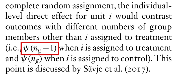
The counterexample. I take two groups of four units and set yig(z)=∑j≠izjy_{ig}(\mathbf{z})=\sum_{j\neq i}z_j, the number of treated group members other than ii. Own treatment has no effect, and partial and stratified interference hold. One group, chosen with probability 1/21/2, has saturation ψ=1/2\psi=1/2 and the other has ϕ=1/4\phi=1/4. Each unit is then treated independently with the probability of its group. For a unit in a group with treatment probability pp, each of the three other members is treated with probability pp whatever zz is, so that yig(0;p)=yig(1;p)=3py_{ig}(0;p)=y_{ig}(1;p)=3p. The group averages of the marginal potential outcomes are 3/23/2 at ψ\psi and 3/43/4 at ϕ\phi, both direct effects are 00, and the indirect, total and overall effects are 3/43/4.

Let KK be the number of treated units in a group. Every treated unit has outcome K−1K-1 and every control unit has outcome KK. The treated arm mean is K−1K-1 when K≥1K\ge 1, the control arm mean is KK when K≤3K\le 3, and their difference is −1-1 on every assignment for which both are defined.

The number KK of treated units in a group of four, its probability at each saturation, and the two arm means.
KKProbability at ψ=1/2\psi=1/2Probability at ϕ=1/4\phi=1/4Treated arm meanControl arm mean
01/1681/256undefined0
14/16108/25601
26/1654/25612
34/1612/25623
41/161/2563undefined

By the table, I have

E[y^g(1;ψ)∣K≥1]=4⋅0+6⋅1+4⋅2+1⋅315=1715,E[y^g(0;ψ)∣K≤3]=1⋅0+4⋅1+6⋅2+4⋅315=2815,\begin{aligned} E\bigl[\widehat{y}_g(1;\psi)\mid K\ge 1\bigr]&=\frac{4\cdot 0+6\cdot 1+4\cdot 2+1\cdot 3}{15}=\frac{17}{15},\\ E\bigl[\widehat{y}_g(0;\psi)\mid K\le 3\bigr]&=\frac{1\cdot 0+4\cdot 1+6\cdot 2+4\cdot 3}{15}=\frac{28}{15}, \end{aligned}

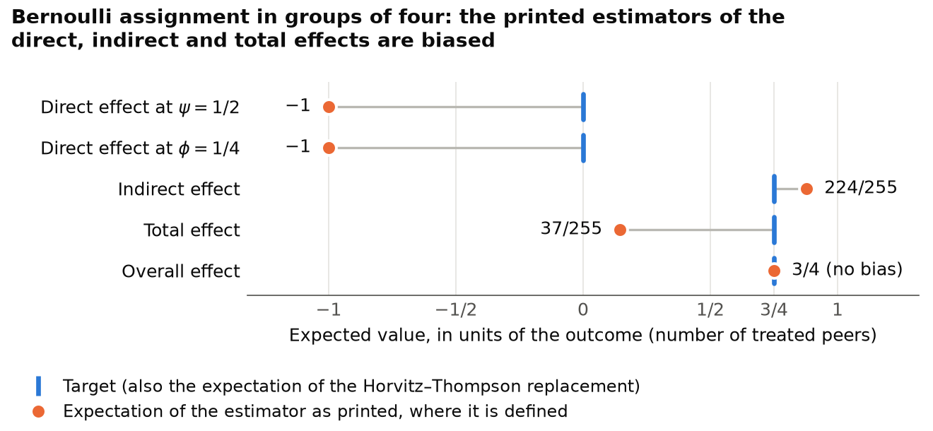
while the target of both is 3/23/2. At ϕ\phi the two conditional expectations are 81/17581/175 and 84/8584/85, and the target is 3/43/4. Enumerating the 512 assignments of the two stages in exact fractions, I find the expectation of each estimator over the assignments on which it is defined. It is −1-1 for τ^D(ψ)\widehat{\tau}^{D}(\psi) and for τ^D(ϕ)\widehat{\tau}^{D}(\phi), whose targets are 00. It is 224/255224/255 for τ^I\widehat{\tau}^{I} and 37/25537/255 for τ^To\widehat{\tau}^{To}, whose targets are 3/43/4. It is 3/43/4 for τ^O\widehat{\tau}^{O}, which equals its target.

The Horvitz–Thompson mean. Since yig(z;ψ)y_{ig}(z;\psi) is the expected outcome of unit ii given Zig=zZ_{ig}=z, I have

E[I(Zig=z) Yig]=Pr⁡(Zig=z) E[Yig∣Zig=z]=ψz(1−ψ)1−z yig(z;ψ).E\bigl[\mathbf{I}(Z_{ig}=z)\,Y_{ig}\bigr]=\Pr(Z_{ig}=z)\,E\bigl[Y_{ig}\mid Z_{ig}=z\bigr]=\psi^{z}(1-\psi)^{1-z}\,y_{ig}(z;\psi).

Summing over ii and dividing by ng ψz(1−ψ)1−zn_g\,\psi^{z}(1-\psi)^{1-z}, I obtain that the Horvitz–Thompson mean in the correction has expectation (1/ng)∑iyig(z;ψ)(1/n_g)\sum_{i}y_{ig}(z;\psi). Note that the expectation is over all assignments, including those with no unit in arm zz, where the sum is 00. In the counterexample, when the arm means are replaced by Horvitz–Thompson means, the expectations found by enumeration equal the targets for all five effects.

Complete random assignment. Suppose that exactly kz≥1k_z\ge 1 units of the group receive treatment zz, all such assignments being equally likely, and let yigcr(z)y^{\mathrm{cr}}_{ig}(z) be the expected outcome of unit ii given Zig=zZ_{ig}=z under this design. Since each unit has treatment zz with probability kz/ngk_z/n_g and the denominator of the arm mean is the constant kzk_z, I find

E[y^g(z;ψ)]=1kz∑i=1ngkzng yigcr(z)=1ng∑i=1ngyigcr(z).E\bigl[\widehat{y}_g(z;\psi)\bigr]=\frac{1}{k_z}\sum_{i=1}^{n_g}\frac{k_z}{n_g}\,y^{\mathrm{cr}}_{ig}(z)=\frac{1}{n_g}\sum_{i=1}^{n_g}y^{\mathrm{cr}}_{ig}(z).

These targets differ from the Bernoulli ones. In the counterexample with two of the four units treated, I have yigcr(1)=1y^{\mathrm{cr}}_{ig}(1)=1 and yigcr(0)=2y^{\mathrm{cr}}_{ig}(0)=2. The direct effect defined for this design is −1-1, while the direct effect under Bernoulli assignment is 00.

Groups. Suppose that a fixed number C≥1C\ge 1 of the GG groups receives saturation ψ\psi, all choices being equally likely. Each group then has saturation ψ\psi with probability C/GC/G. If a quantity computed in group gg has expectation μg\mu_g when the group has saturation ψ\psi, its mean over the groups with that saturation has expectation (1/G)∑gμg(1/G)\sum_{g}\mu_g. Applied to the Horvitz–Thompson means and to the arm means under complete random assignment, this implies the population statements in the correction. Applied to the mean outcome of all units in a group, it implies that τ^O\widehat{\tau}^{O} is unbiased.

What survives

The definitions of the marginal causal effects on p. 309 and the estimator of the overall effect are unaffected. The toy example on pp. 310–311 uses complete random assignment in both stages, and Figure 16.6 uses the same two-stage design. For that design the arm means are unbiased for the marginal potential outcomes defined by it. No reported number is known to depend on the claim. What changes is that, under Bernoulli assignment within groups, the printed estimators of the direct, indirect and total effects cannot be called unbiased. No variance estimator for the Horvitz–Thompson means was derived.

Corrected

Let the observed outcome be Yig=yig(Zig)Y_{ig}=y_{ig}(\mathbf{Z}_{ig}) under the group treatment assignment Zig\mathbf{Z}_{ig} and suppose treatment saturation is ψ\psi, with 0<ψ<10<\psi<1 and, for the indirect and total contrasts, 0≤ϕ<1\colorbox{#ffe58a}{$0\le\phi<1$}. Given Bernoulli assignment with probability ψ\psi, the arm mean

y^g(z;ψ)=∑i=1ngYigI(Zig=z)∑i=1ngI(Zig=z)\widehat{y}_g(z;\psi)=\frac{\sum_{i=1}^{n_g}Y_{ig}\mathbf{I}(Z_{ig}=z)}{\sum_{i=1}^{n_g}\mathbf{I}(Z_{ig}=z)}

is not in general unbiased for 1ng∑i=1ngyig(z;ψ)\frac{1}{n_g}\sum_{i=1}^{n_g}y_{ig}(z;\psi), with z∈{0,1}z\in\{0,1\}, even conditional on its denominator being nonzero. An unbiased estimator is

y^gHT(z;ψ)=∑i=1ngYigI(Zig=z)ng ψz(1−ψ)1−z,\widehat{y}^{HT}_g(z;\psi)=\frac{\sum_{i=1}^{n_g}Y_{ig}\mathbf{I}(Z_{ig}=z)}{\colorbox{#ffe58a}{$\displaystyle n_g\,\psi^{z}(1-\psi)^{1-z}$}},

computed for every assignment, with the value 00 when no unit of the group has treatment zz. Suppose that a fixed positive number of the GG groups is assigned to each saturation, all such assignments being equally likely. Then

y^HT(z;ψ)=∑g=1Gy^gHT(z;ψ)I(Sg=ψ)∑g=1GI(Sg=ψ),\widehat{y}^{HT}(z;\psi)=\frac{\sum_{g=1}^{G}\widehat{y}^{HT}_g(z;\psi)\mathbf{I}(S_g=\psi)}{\sum_{g=1}^{G}\mathbf{I}(S_g=\psi)},

where SgS_g is the saturation level of group gg, is unbiased for the population average potential outcome. The estimators τ^D(ψ)=y^HT(1;ψ)−y^HT(0;ψ)\widehat{\tau}^{D}(\psi)=\widehat{y}^{HT}(1;\psi)-\widehat{y}^{HT}(0;\psi), τ^I(ψ,ϕ)=y^HT(0;ψ)−y^HT(0;ϕ)\widehat{\tau}^{I}(\psi,\phi)=\widehat{y}^{HT}(0;\psi)-\widehat{y}^{HT}(0;\phi) and τ^To(ψ,ϕ)=y^HT(1;ψ)−y^HT(0;ϕ)\widehat{\tau}^{To}(\psi,\phi)=\widehat{y}^{HT}(1;\psi)-\widehat{y}^{HT}(0;\phi) are then unbiased for the average direct, indirect and total effects. The estimator τ^O(ψ,ϕ)=y^(ψ)−y^(ϕ)\widehat{\tau}^{O}(\psi,\phi)=\widehat{y}(\psi)-\widehat{y}(\phi), where y^(ψ)\widehat{y}(\psi) is the average across groups assigned to saturation ψ\psi of the average observed outcomes of units in the group, is unbiased for the average overall effect.

Alternatively, suppose that treatment within each group is by complete random assignment, with a fixed number of treated units and a fixed number of control units, both at least one, and that the marginal potential outcomes yig(z;ψ)y_{ig}(z;\psi) are defined by averaging over the assignments of that design. Then the arm means y^g(z;ψ)\widehat{y}_g(z;\psi) and y^(z;ψ)\widehat{y}(z;\psi) as printed, and the estimators τ^D\widehat{\tau}^{D}, τ^I\widehat{\tau}^{I} and τ^To\widehat{\tau}^{To} built from them, are unbiased for the corresponding quantities under the same assignment of groups to saturations.

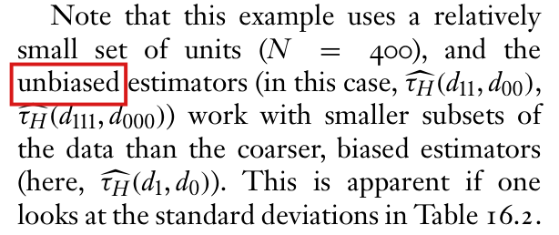
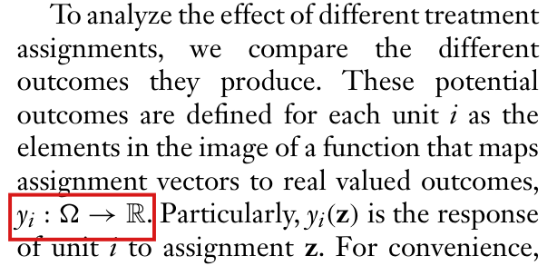
Six lines of text followed by a displayed formula. A red box marks the word 'unbiased' in the sentence 'Given Bernoulli assignment with probability psi, an unbiased estimator for one over n_g times the sum of y_ig(z; psi), with z = {0, 1}, is'. The display below defines y-hat_g(z; psi) as the sum of Y_ig times the indicator of Z_ig = z, divided by the sum of the indicators.
Section 16.5.1, p. 310 (PDF p. 22), left column: the sentence that calls the arm mean y^g(z;ψ)\widehat{y}_g(z;\psi) unbiased under Bernoulli assignment, with “unbiased” marked, and the display that defines the arm mean.
Nine lines of text. Red boxes mark the word 'unbiased' in 'Therefore, an unbiased estimator for the average direct effect is tau-hat D(psi) = y-hat(1; psi) minus y-hat(0; psi)' and the word 'Unbiased' that begins the next sentence, 'Unbiased estimators for the other causal estimands of interest are defined analogously'.
Section 16.5.1, p. 310 (PDF p. 22), left column, below the second display: the sentences that call the estimators of the direct, indirect, total and overall effects unbiased, with “unbiased” and “Unbiased” marked.
A chart with five rows and a horizontal axis of expected value from minus 1 to 1. Blue vertical ticks mark the targets: 0 for the direct effect at psi = 1/2 and for the direct effect at phi = 1/4, and 3/4 for the indirect, total and overall effects. Orange dots mark the expectation of each estimator as printed: minus 1 for each direct effect, 224/255 for the indirect effect, 37/255 for the total effect, and 3/4 for the overall effect, where the dot lies on the tick and is labelled 'no bias'. In the first four rows a grey line joins the dot to its tick. The legend says that the tick is also the expectation of the Horvitz-Thompson replacement.
Targets and expectations in the counterexample of this finding: two groups of four units, outcome equal to the number of treated group members other than the unit, one group at ψ=1/2\psi=1/2 and one at ϕ=1/4\phi=1/4, Bernoulli assignment within groups. The expectations of the printed estimators are conditional on each estimator being defined; all values are exact fractions from enumeration of 512 assignments. The Horvitz–Thompson replacements have unconditional expectations equal to the targets; the overall estimator is unchanged.

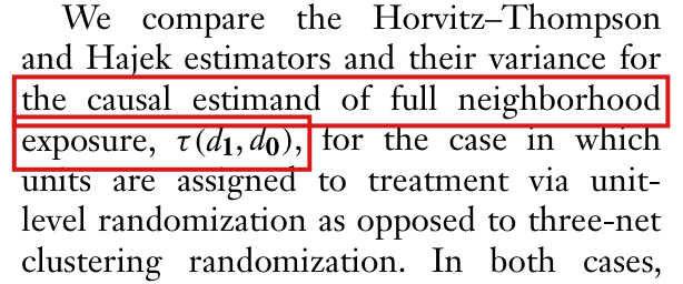
The package’s full-neighborhood exposure mapping must code a unit as all control when no member of its closed neighborhood is treated; as written it codes every unit whose closed neighborhood is not entirely treated as all control, so that the contrast it supports is not the τ(d1,d0)\tau(d_{\mathbf{1}},d_{\mathbf{0}}) of Section 16.4.6.

Section 16.4.6 and Table 16.3, p. 305 (PDF p. 17); lines 104–121 of the file R/make_exposure_map_AS.R in the R package interference, version 0.1.0 (code, not printed in the chapter)

See also under Formal statements (Lean): P045-T5, P045-T6, P045-T27

As printed

Section 16.4.6, p. 305: “We compare the Horvitz–Thompson and Hajek estimators and their variance for the causal estimand of full neighborhood exposure, τ(d1,d0)\tau(d_{\mathbf{1}},d_{\mathbf{0}}), for the case in which units are assigned to treatment via unit-level randomization as opposed to three-net clustering randomization.”

Package, documentation of make_exposure_map_full_neighborhood: “that produces two exposure conditions: All Treat; a unit and 100% of its first-degree neighbors are treated, and All Control; a unit and 100% of its first-degree neighbors are in the control condition.”

Package, R/make_exposure_map_AS.R, lines 116–120.
LineCode
116exposure <- as.numeric(tr_vector%*%adj_matrix_diag)
117B_size <- rowSums(adj_matrix_diag)
118return(matrix(as.numeric(c(exposure==B_size,
119    exposure<B_size)),
120  N, 2, dimnames = list(NULL, c('all_treat', 'all_control'))))
The problem

Section 16.4.6 and Table 16.3 concern the contrast τ(d1,d0)\tau(d_{\mathbf{1}},d_{\mathbf{0}}) between two exposure conditions: a unit and all of its first-degree neighbors are treated, and a unit and all of its first-degree neighbors are in control. The section motivates it on p. 304 by the difference between 100% and 0% treatment saturation. The package has one exposure mapping for these two conditions, and its documentation describes them in the same way. Its second indicator is exposure<B_size, where exposure is the number of treated units in the closed neighborhood of a unit (the unit and its first-degree neighbors) and B_size is the size of that neighborhood. This indicator is one whenever at least one member of the closed neighborhood is untreated. Then a unit whose closed neighborhood is partly treated is coded all control, and so is a treated unit with one untreated neighbor. The contrast that the function supports is between a closed neighborhood that is entirely treated and everything else.

Every quantity that the package computes for the comparison condition inherits the wrong event: its exposure probability, the inverse-probability weights, the comparison mean and the variance estimates. When the outcomes in a partly treated neighborhood differ from the outcomes under full control, the Horvitz–Thompson contrast built on the function’s two indicators can estimate a different quantity from τ(d1,d0)\tau(d_{\mathbf{1}},d_{\mathbf{0}}), and nothing in the output shows it. Whether Table 16.3 was computed with this function is not known, because the script that produced the table is not in the replication files. No entry of Table 16.3 is shown to be wrong. If every unit short of full treatment has its baseline outcome, then the contrast built on the function’s indicators has the same expectation as the intended one.

Evidence an exact counterexample

The evidence is a derivation and an exact counterexample. For the derivation, consider an undirected network without loops, with adjacency matrix AA, and a treatment vector z\mathbf{z} with entries 0 and 1. For each unit ii, let Bi={i}∪{j:Aij=1}B_i=\{i\}\cup\{j:A_{ij}=1\} be its closed neighborhood, let bi=∣Bi∣b_i=|B_i|, and let si=∑j∈Bizjs_i=\sum_{j\in B_i}z_j. Lines 114–117 compute exposure =si=s_i and B_size =bi=b_i. Since 0≤si≤bi0\le s_i\le b_i, I have si=bis_i=b_i exactly when every member of BiB_i is treated and si=0s_i=0 exactly when no member is treated. The condition si<bis_i<b_i holds exactly when at least one member is untreated, and it includes every case with 0<si<bi0<s_i<b_i. Note that the first indicator of the function is correct and that the second is the complement of the first.

For the counterexample, let two units be joined by one tie, so that b1=b2=2b_1=b_2=2. For the assignment z=(1,0)\mathbf{z}=(1,0), I have s1=s2=1s_1=s_2=1. The function, run unchanged from both copies of the package in the replication files, returns (all treated, all control) =(0,1)=(0,1) for both units, and the documented conditions give (0,0)(0,0). Let the two units be treated independently with probability 1/21/2. Each unit is all treated with probability 1/41/4, all control with probability 1/41/4, and coded all control by the function with probability 3/43/4. Let both units have outcome Yi(z)=1+z1+z2Y_i(\mathbf{z})=1+z_1+z_2, so that τ(d1,d0)=3−1=2\tau(d_{\mathbf{1}},d_{\mathbf{0}})=3-1=2. The table lists the Horvitz–Thompson contrast of p. 297 for each assignment, with exact probabilities. Its expectation is 4/34/3 with the function’s events and 22 with the documented events.

Two units joined by one tie, treated independently with probability 1/21/2, with outcomes Yi(z)=1+z1+z2Y_i(\mathbf{z})=1+z_1+z_2. Columns 3 and 4 give the pair (all treated, all control), which is the same for both units, from the function as written and from the documented conditions. Columns 5 and 6 give the Horvitz–Thompson contrast with the events of the function as written and with the documented events.
(z1,z2)(z_1,z_2)sis_iPair, as writtenPair, documentedContrast, as writtenContrast, documented
(0,0)(0,0)0(0,1)(0,1)(0,1)(0,1)−4/3-4/3−4-4
(0,1)(0,1)1(0,1)(0,1)(0,0)(0,0)−8/3-8/300
(1,0)(1,0)1(0,1)(0,1)(0,0)(0,0)−8/3-8/300
(1,1)(1,1)2(1,0)(1,0)(1,0)(1,0)12121212
Expectation4/34/322

With the threshold outcomes Yi(z)=1+2 I(z1=z2=1)Y_i(\mathbf{z})=1+2\,\mathbf{I}(z_1=z_2=1), the contrast is again 22, and both versions of the estimator have expectation 22. This is why the defect does not by itself imply an error in Table 16.3. Over all simple undirected networks on one to four labeled units and all treatment vectors, 1098 configurations in total, the function as written gets 2456 of the 4306 unit classifications wrong, and the corrected indicator agrees with a direct check of the treatment of every member of BiB_i in every case.

What survives

The indicator for a closed neighborhood that is entirely treated is correct, and the package’s mapping into the four conditions d11d_{11}, d10d_{10}, d01d_{01} and d00d_{00} is a separate function. The estimators and their theory for a correctly specified exposure mapping, and the argument of Section 16.4.6 for designs that raise the probability of the two full-neighborhood conditions, are unaffected. No entry of Table 16.3 and no ranking in it is shown to be wrong. The function changes, and outputs that use its all-control indicator have to be computed again with the corrected event. The package’s 3-net sampler is the subject of P045-E013.

Corrected
Package, R/make_exposure_map_AS.R, lines 118–120, corrected.
LineCode
118return(matrix(as.numeric(c(exposure==B_size,
119    exposure==0)),
120  N, 2, dimnames = list(NULL, c('all_treat', 'all_control'))))

For an undirected network without loops, the function then returns I(si=bi)\mathbf{I}(s_i=b_i) and I(si=0)\mathbf{I}(s_i=0): a unit is all treated when every member of its closed neighborhood is treated and all control when none is. A unit with a partly treated closed neighborhood is in neither condition, so the two columns no longer sum to one. Recompute exposure probabilities and weights from the corrected events, retaining the original population size and observed outcomes. In simulations, code that uses the two columns to generate outcomes, as the package’s example does, must assign mixed-neighborhood outcomes from its outcome model rather than turn them into zeros.

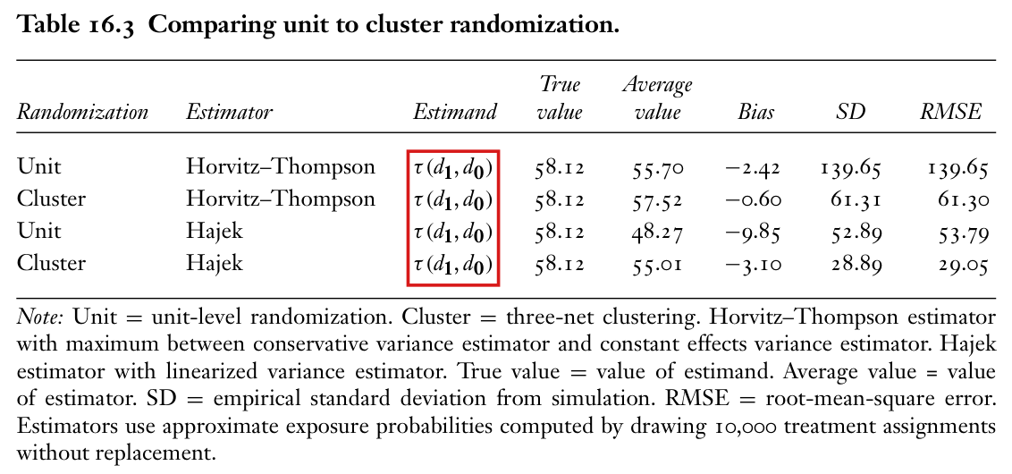
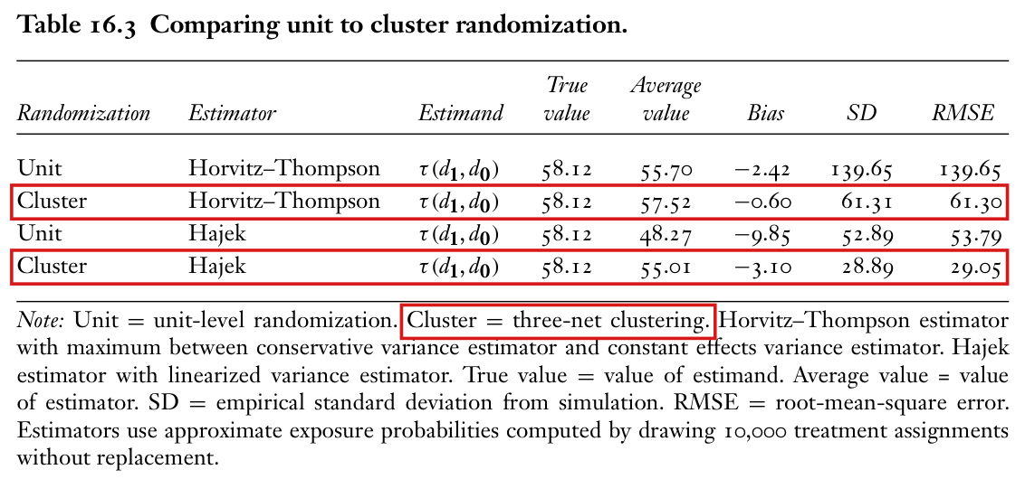
Crop of Table 16.3 on page 305, 'Comparing unit to cluster randomization', with columns Randomization, Estimator, Estimand, True value, Average value, Bias, SD and RMSE, four rows (Unit and Cluster for Horvitz-Thompson, Unit and Cluster for Hajek) and the note below the table. A red box marks the Estimand column, which reads tau(d1, d0) in all four rows.
Table 16.3, p. 305 (PDF p. 17). The marked column gives the estimand, the contrast τ(d1,d0)\tau(d_{\mathbf{1}},d_{\mathbf{0}}) between the two full-neighborhood exposure conditions.
Crop of seven lines from the right column of page 305. The text reads 'We compare the Horvitz-Thompson and Hajek estimators and their variance for the causal estimand of full neighborhood exposure, tau(d1, d0), for the case in which units are assigned to treatment via unit-level randomization as opposed to three-net clustering randomization. In both cases,'. Red boxes mark the words 'the causal estimand of full neighborhood' and 'exposure, tau(d1, d0),'.
Section 16.4.6, p. 305 (PDF p. 17), right column. The marked words name the estimand of Table 16.3.

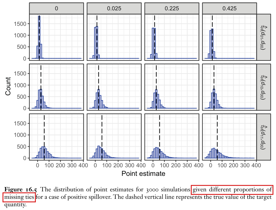
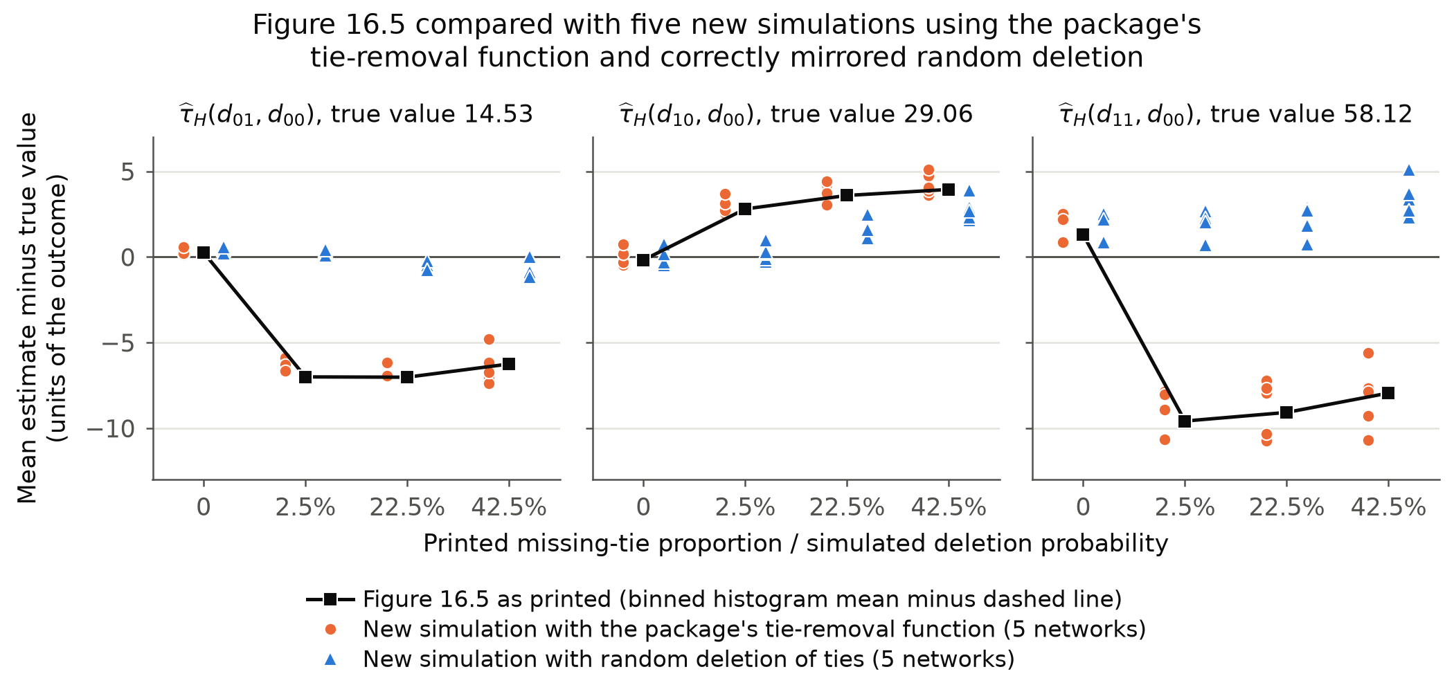
The package’s functions for removing and for adding ties must copy the transpose of the edited upper triangle; as written they in general return an asymmetric network with ties that were never there, Figure 16.5 resembles simulations using these functions although its generating code is unknown, and the general statement on p. 303 that the bias increases with the proportion of mismeasured ties needs qualifying.

Figure 16.5, p. 304 (PDF p. 16), and Section 16.4.4, p. 303 (PDF p. 15), right column; lines 36 and 55 of the file R/functions.R in the R package interference, version 0.1.0 (code, not printed in the chapter)

See also under Formal statements (Lean): P045-T7, P045-T8, P045-T9

Revised: see the history of this entry.

As printed

Package, file R/functions.R, line 36 in the function make_adj_matrix_trunc, which removes ties, and line 55 in the function make_adj_matrix_add, which adds ties:

m[lower.tri(m,diag=FALSE)] <- m[upper.tri(m,diag=FALSE)]

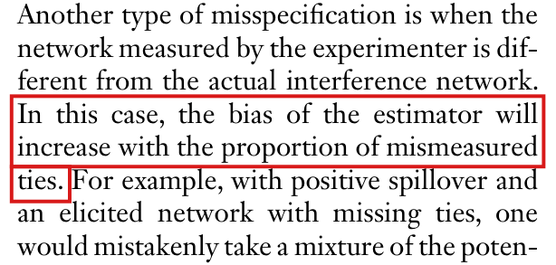
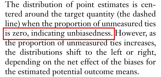
Section 16.4.4, p. 303: “In this case, the bias of the estimator will increase with the proportion of mismeasured ties.” and “The distribution of point estimates is centered around the target quantity (the dashed line) when the proportion of unmeasured ties is zero, indicating unbiasedness. However, as the proportion of unmeasured ties increases, the distributions shift to the left or right, depending on the net effect of the biases for the estimated potential outcome means.”
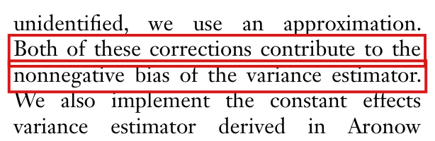
Figure 16.5, p. 304, caption: “The distribution of point estimates for 3000 simulations given different proportions of missing ties for a case of positive spillover. The dashed vertical line represents the true value of the target quantity.”
The problem

Section 16.4.4 asks what happens when the measured network misses some ties of the interference network, and Figure 16.5 illustrates this. The package provides a function intended to remove each tie with probability p and a function that adds ties. Both edit the upper triangle of the adjacency matrix and then copy the upper triangle into the lower triangle with the line above. R lists the cells of each triangle column by column, and in that order the kkth cell of the upper triangle is in general not the transpose of the kkth cell of the lower triangle. The matrix that the functions return is in general not symmetric. It can lack entries that were not removed and contain entries that were never in the network. A simulation that removes ties with this function studies the altered network, and not a network from which a random share of the ties is missing.
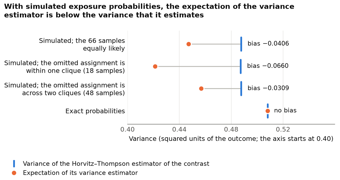
The printed figure has the pattern that the altered network produces, although this does not show that it was drawn with the defective function. Reading the histograms from the drawing of the page, I find that the binned mean estimate lies about 7.07.0 below the true value 14.5314.53 of τ(d01,d00)\tau(d_{01},d_{00}) and 9.69.6 below the true value 58.1258.12 of τ(d11,d00)\tau(d_{11},d_{00}) in the column labelled 0.025. The binned gaps are about as large in the columns labelled 0.225 and 0.425. I simulated the stated design on five networks. With the package’s tie-removal function the same jump appears at a deletion probability of 2.5%. With correctly mirrored random deletion, the average changes in the three contrasts, using experiments where both estimates are defined, are less than 0.30.3 in magnitude at 2.5%, at most 1.81.8 at 22.5% and at most 3.23.2 at 42.5%. The printed binned offsets at 2.5% are much larger than any change at that probability in these five simulations. Since the simulations use new networks, and the bins of the figure are about 14.4 wide, this comparison does not measure how far the figure departs from the effect of random deletion on its own network. The script that drew the figure is not in the replication files. The five simulations support the attribution of the figure to the tie-removal function, and they do not establish it; an example below shows that the deletion of particular ties, 2.5% of the total, can produce shifts of this size.

The sentence that opens the section, that the bias of the estimator will increase with the proportion of mismeasured ties, is stated generally, before the figure is introduced, and it needs qualifying: the bias need not increase. In an exact example below, the absolute bias of the Hajek contrast decreases when ties are deleted at random. That example concerns the total bias of the estimator in a small network. It does not show that the simulation of Figure 16.5 behaves otherwise than the chapter describes, or that the part of the bias due to the missing ties decreases.

The words “indicating unbiasedness” describe the centring of the histograms in one figure. Page 299 already says that the Hajek estimator improves efficiency “with a small cost in terms of finite-sample bias”, and Table 16.1, p. 300 (PDF p. 12), reports biases of 0.320.32, −0.14-0.14 and 1.291.29 for these three estimators with no missing ties. Read with that qualification, the words say that the figure shows no appreciable bias, not that the estimator is exactly unbiased. They call for a clarification, below, and are not part of the error.

Evidence an exact counterexample

The evidence is an exact counterexample for the code, a derivation for the repair, a reading of the printed figure, new simulations, and two exact examples that mark the limits of the conclusion.

The code. Let AA be the adjacency matrix of the network on four units whose only tie joins units 1 and 4. Each of the two functions, called with p=0p=0, leaves the upper triangle unchanged and returns the matrix BB:

A=(0001000000001000),B=(0001000001000000).A=\begin{pmatrix}0&0&0&1\\0&0&0&0\\0&0&0&0\\1&0&0&0\end{pmatrix},\qquad B=\begin{pmatrix}0&0&0&1\\0&0&0&0\\0&1&0&0\\0&0&0&0\end{pmatrix}.

R lists the upper cells in the order (1,2),(1,3),(2,3),(1,4),(2,4),(3,4)(1,2),(1,3),(2,3),(1,4),(2,4),(3,4) and the lower cells in the order (2,1),(3,1),(4,1),(3,2),(4,2),(4,3)(2,1),(3,1),(4,1),(3,2),(4,2),(4,3). The fourth upper cell, (1,4)(1,4), is written to the fourth lower cell, (3,2)(3,2), and not to (4,1)(4,1). The matrix BB is not symmetric: the entry (3,2)(3,2) was added and the entry (4,1)(4,1) was removed. The same BB is returned through the package’s function make_adj_matrix_miss_ties with p=1/40p=1/40 and seed 1, for removal and for addition. With BB in place of AA, the exposure mapping of the package moves unit 1 from d01d_{01} to d00d_{00} when unit 4 alone is treated, and it moves unit 2 from d00d_{00} to d01d_{01} when unit 3 alone is treated. Over all 64 upper triangles on four units, the printed line returns an asymmetric matrix for 32, and the corrected line returns the symmetric matrix for all 64. On the network of ten units that is printed on p. 295, the tie-removal function with p=9/40p=9/40 and seed 56 removes 4 ties from the upper triangle, and its output differs from the input by 9 added and 17 removed entries.

The repair. Let UU be the upper triangle after the random edits, with zeros elsewhere. The corrected line writes mjim_{ji} to each lower cell (i,j)(i,j) such that i>ji>j, and it changes no cell on or above the diagonal. The result is U+UTU+U^{\mathsf T}, which is symmetric. For a symmetric input AA with entries 0 and 1 and zero diagonal, and upper cells i<ji<j, I have 0≤Uij≤Aij0\le U_{ij}\le A_{ij} after a removal, so that no entry is added, and Aij≤Uij≤1A_{ij}\le U_{ij}\le 1 after an addition, so that no entry is removed.

The printed figure. Figure 16.5 is a vector drawing, and the heights of its bars give the counts of each histogram; the counts of each of the twelve panels sum to 3000. The third column of the table below is the mean of each histogram minus the position of its dashed line. The bins are about 14.4 wide, so these means are those of the binned estimates.

New simulations. I drew five networks of 400 units and 800 ties with the package’s generator and simulated the design of pp. 299 and 303: 40 treated units, dilated effects, Hajek estimators, 10,000 draws for the exposure probabilities and 3000 experiments. For each network and each deletion probability, I measured the network once with the package’s tie-removal function and once after mirroring the same random deletion decisions correctly. At a deletion probability of 2.5% the tie-removal function deleted between 13 and 21 ties, and its output contained between 766 and 780 entries that were not in the network. The last two columns of the table give the range, over the five networks, of the mean of the defined estimates minus each network’s true value. Averaging changes from no missing ties over experiments where both estimates are defined, random deletion at probability 2.5% moves τH^(d01,d00)\widehat{\tau_H}(d_{01},d_{00}) by −0.19-0.19 to +0.09+0.09, τH^(d10,d00)\widehat{\tau_H}(d_{10},d_{00}) by +0.04+0.04 to +0.25+0.25 and τH^(d11,d00)\widehat{\tau_H}(d_{11},d_{00}) by −0.25-0.25 to +0.10+0.10. The tie-removal function moves them by −7.22-7.22 to −6.29-6.29, by +2.96+2.96 to +3.41+3.41 and by −11.53-11.53 to −10.45-10.45.

Binned histogram mean minus dashed-line position in Figure 16.5, and mean estimate minus each network’s true value over five new simulations, in units of the outcome.
EstimatorPrinted proportion / deletion probabilityFigure 16.5 as printedTie-removal functionRandom deletion
τH^(d01,d00)\widehat{\tau_H}(d_{01},d_{00})0+0.260+0.260+0.130+0.130 to +0.560+0.560+0.130+0.130 to +0.560+0.560
2.5%−7.008-7.008−6.663-6.663 to −5.891-5.891+0.045+0.045 to +0.404+0.404
22.5%−7.026-7.026−6.965-6.965 to −6.113-6.113−0.841-0.841 to −0.242-0.242
42.5%−6.256-6.256−7.364-7.364 to −4.817-4.817−1.154-1.154 to +0.026+0.026
τH^(d10,d00)\widehat{\tau_H}(d_{10},d_{00})0−0.187-0.187−0.459-0.459 to +0.731+0.731−0.459-0.459 to +0.731+0.731
2.5%+2.798+2.798+2.540+2.540 to +3.699+3.699−0.265-0.265 to +0.985+0.985
22.5%+3.586+3.586+3.060+3.060 to +4.429+4.429+1.094+1.094 to +2.475+2.475
42.5%+3.937+3.937+3.591+3.591 to +5.117+5.117+2.167+2.167 to +3.891+3.891
τH^(d11,d00)\widehat{\tau_H}(d_{11},d_{00})0+1.299+1.299+0.861+0.861 to +2.679+2.679+0.861+0.861 to +2.679+2.679
2.5%−9.587-9.587−10.671-10.671 to −7.854-7.854+0.715+0.715 to +2.739+2.739
22.5%−9.082-9.082−10.742-10.742 to −7.218-7.218+0.739+0.739 to +2.895+2.895
42.5%−7.952-7.952−10.716-10.716 to −5.598-5.598+2.303+2.303 to +5.096+5.096

Limits. The simulations use new networks and new outcomes, since the network, the outcomes and the script of the printed figure are not available. They do not give the values of a corrected figure. They also do not exclude random deletion as the source of the printed figure. Let 400 units form eighty groups of five, with a tie between every two units of a group. Let the baseline outcome be 250 in two of the groups and 53.2 in the others, so that the mean baseline is 58.12. Suppose that the 20 missing ties, out of 800, are exactly the ties within the two groups with the high baseline. With exact exposure probabilities and conditioning separately on each contrast being defined, an exact calculation yields a bias of −6.70-6.70 for τH^(d01,d00)\widehat{\tau_H}(d_{01},d_{00}) and of −10.39-10.39 for τH^(d11,d00)\widehat{\tau_H}(d_{11},d_{00}). Configurations arbitrarily close to this example have positive but very small probability under the stated stochastic design.

Bias and the proportion of missing ties. On the ten-unit network of p. 295, let one unit be treated, chosen uniformly, and let the baseline outcome be 5/25/2 for unit 2 and 11 for the other units, with the multipliers of p. 298. Enumerating every assignment and every set of deleted ties in exact arithmetic, I find that the bias of τH^(d01,d00)\widehat{\tau_H}(d_{01},d_{00}) is +0.0200+0.0200 with no tie deleted, +0.0091+0.0091 with one of the 20 ties deleted at random and −0.0012-0.0012 with two deleted. The absolute bias decreases. This is the total bias of the contrast in one small design: it qualifies the general statement on p. 303 and says nothing about the simulation of Figure 16.5.

What survives

The estimands, the exposure conditions and the estimator formulas do not depend on the two functions. The point of the section, that mismeasured ties can bias the estimators, stands. The column of Figure 16.5 with no missing ties is not in question: the package’s make_adj_matrix_miss_ties function with p=0p=0 and type nothing returns the network unchanged, and the printed histograms are approximately centered, in agreement with Table 16.1. No other table or figure is shown to depend on the two functions. What changes is the code, the confidence in reading the three other columns of Figure 16.5 as the effect of random deletion at the stated proportions, and the general statement on p. 303 about increasing bias. The words “indicating unbiasedness” need only the clarification below.

Corrected

Package, R/functions.R, lines 36 and 55:

m[lower.tri(m,diag=FALSE)] <- t(m)[lower.tri(m,diag=FALSE)]

For a symmetric adjacency matrix with entries 0 and 1 and zero diagonal, and defined, admissible edit probabilities, the two functions then return a symmetric matrix in which ties are only removed, or only added.

Section 16.4.4, p. 303: “In this case, missing or mismeasured ties can introduce bias, whose magnitude need not increase monotonically with the proportion of missing ties.”

As a clarification, the description of Figure 16.5 can read: “The distribution of point estimates is approximately centered around the target quantity (the dashed line) when the proportion of unmeasured ties is zero; the Hajek estimator can still have a small finite-sample bias.”

If Figure 16.5 was drawn with either defective function, it must be drawn again with the corrected code. Whether it was is not established: its original inputs and generating code are needed to determine whether its columns 0.025, 0.225 and 0.425 show the effect of random deletion of ties.

Crop of Figure 16.5 on page 304: twelve histograms of point estimates in three rows, for tau-hat H of d01, d00, of d10, d00 and of d11, d00, and four columns headed 0, 0.025, 0.225 and 0.425, each with a dashed vertical line at the true value. In the first and third rows the histograms of the three right-hand columns sit to the left of the dashed line by a similar amount. The caption reads 'Figure 16.5 The distribution of point estimates for 3000 simulations given different proportions of missing ties for a case of positive spillover. The dashed vertical line represents the true value of the target quantity.' Red boxes mark the words 'given different proportions of' and 'missing ties'.
Figure 16.5, p. 304 (PDF p. 16). The columns are labelled 0, 0.025, 0.225 and 0.425 as proportions of missing ties. The marked words describe the intended simulation.
Crop of eight lines from the right column of page 303. The text reads 'Another type of misspecification is when the network measured by the experimenter is different from the actual interference network. In this case, the bias of the estimator will increase with the proportion of mismeasured ties. For example, with positive spillover and an elicited network with missing ties, one would mistakenly take a mixture of the poten-'. Red boxes mark the sentence 'In this case, the bias of the estimator will increase with the proportion of mismeasured ties.'
Section 16.4.4, p. 303 (PDF p. 15), right column, opening of the section. The marked sentence says that the bias increases with the proportion of mismeasured ties.
Crop of eight lines from the right column of page 303. The text reads 'The distribution of point estimates is centered around the target quantity (the dashed line) when the proportion of unmeasured ties is zero, indicating unbiasedness. However, as the proportion of unmeasured ties increases, the distributions shift to the left or right, depending on the net effect of the biases for the estimated potential outcome means.' A red box marks the words 'is zero, indicating unbiasedness.'
Section 16.4.4, p. 303 (PDF p. 15), right column, the description of Figure 16.5. The marked words are “is zero, indicating unbiasedness.”
The title reads 'Figure 16.5 compared with five new simulations using the package's tie-removal function and correctly mirrored random deletion'. Three panels, one for each of tau-hat H of d01, d00, of d10, d00 and of d11, d00. Titles give the printed targets 14.53, 29.06 and 58.12; simulation targets vary by network. Horizontal positions are labelled 0, 2.5 percent, 22.5 percent and 42.5 percent, under the axis label 'Printed missing-tie proportion / simulated deletion probability'; for the simulations these are deletion probabilities, not realized missing shares. The vertical axis runs from minus 13 to 7 units of the outcome. Black squares joined by a line show printed binned means minus dashed-line positions: for d01 about 0.3, minus 7.0, minus 7.0 and minus 6.3; for d10 about minus 0.2, 2.8, 3.6 and 3.9; for d11 about 1.3, minus 9.6, minus 9.1 and minus 8.0. Orange circles and blue triangles, five per position, show simulation means minus each network's true target. Orange circles generally follow the printed pattern. Blue triangles change little at 2.5 percent; by 42.5 percent they range from minus 1.2 to 0.0 for d01, from 2.2 to 3.9 for d10 and from 2.3 to 5.1 for d11.
Comparison for the three contrasts of Figure 16.5. Black squares: printed binned histogram mean minus dashed-line position. Orange circles: new simulations with the package’s tie-removal function, one point per network. Blue triangles: new simulations with random deletion of ties, mirrored correctly. Simulation values subtract each network’s own true value; their horizontal positions denote deletion probabilities. The comparison supports but does not establish the source of the printed figure.
History of this entry
  1. Classification before my review (the classification when the audit was first completed, before I reviewed it): Moderate error.
  2. Revised. The wording was revised; the classification remains a Moderate error. The package’s tie-editing functions are defective independently of how the prose is read. The description of approximate centering needs clarification because the Hajek estimator can have small finite-sample bias, and the general claim that bias increases with missing ties needs qualification. The evidence supports but does not establish that the defective functions generated Figure 16.5; its original inputs and generating code are needed to settle that attribution.

The package’s 3-net sampler must draw each new center by index from the unmarked units; as written it draws from 1,…,n1,\dots,n when a single unmarked unit nn remains, and in new simulations of the design of Table 16.3 it returns centers closer than three hops in about nine clusterings out of ten.

Table 16.3, rows Cluster, and Section 16.4.6, p. 305 (PDF p. 17); the file R/make_tr_vec_bernoulli.R, lines 77 and 123, in the R package interference, version 0.1.0 (code, not printed in the chapter)

See also under Formal statements (Lean): P045-T10, P045-T11, P045-T29

As printed
Table 16.3, p. 305, rows Cluster.
RandomizationEstimatorEstimandTrue valueAverage valueBiasSDRMSE
ClusterHorvitz–Thompsonτ(d1,d0)\tau(d_1,d_0)58.1257.52−0.60-0.6061.3161.30
ClusterHajekτ(d1,d0)\tau(d_1,d_0)58.1255.01−3.10-3.1028.8929.05

Table 16.3, note: “Unit = unit-level randomization. Cluster = three-net clustering.”

Package, R/make_tr_vec_bernoulli.R, lines 76–82. Lines 122–128 repeat the loop.
LineCode
76while (any(!marked)) {
77  v_j <- sample(which(!marked), 1)
78  cluster_centers[v_j] <- j
79  marked[v_j]  <- TRUE
80  marked[unlist(B_2[v_j])]  <- TRUE
81  j <- j + 1
82}
The problem

Table 16.3 compares unit-level randomization with cluster randomization, where the clusters come from 3-net clustering: the centers are at least three hops apart, every unit is within two hops of a center, each unit joins a nearest center, and treatment is assigned by cluster. The package’s sampler builds the centers in a loop. It draws a center from the units that are not yet marked, marks the center and every unit within two hops of it, and repeats until every unit is marked. The draw is sample(which(!marked), 1). When exactly one unmarked unit nn remains, which(!marked) is the single number nn, and R then draws uniformly from 1,…,n1,\dots,n and not from the one remaining unit. Each draw that misses the units within two hops of nn writes a center on a unit that is already marked. Unless that unit is already a center, the new center lies within two hops of an earlier one. The loop continues until a draw lands within two hops of nn.

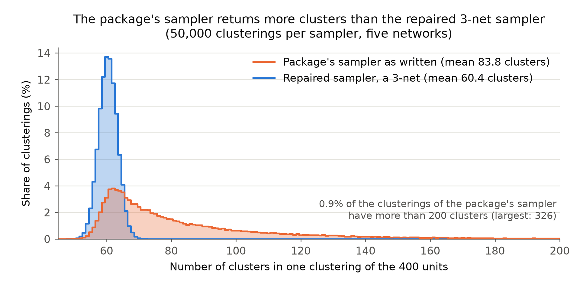
This is not a rare case in new simulations of the design of Table 16.3. In 50,000 clusterings of five networks of 400 units, the loop reached a single unmarked unit n>1n>1 in 92.75% of the clusterings, and the final centers were closer than three hops in 91.17%. The sampler as written returned 83.8 clusters on average, against 60.4 for the repaired sampler, and the estimated probability that the closed neighborhood of a unit is entirely treated, averaged over units, was 0.169, against 0.193. The design that the package draws under the name of 3-net clustering is therefore a different design. If the rows Cluster of Table 16.3 were computed with the package, they are not results for 3-net clustering. The script and the seeds of the table are not in the replication files, and no printed entry is shown to be wrong. In the new simulations the repaired sampler has estimated standard deviations that are lower by 4% to 14%.

Evidence an exact counterexample

The evidence is an exact counterexample, a derivation, and new simulations of the design of Table 16.3.

Counterexample. Let four units form the path 11–22–33–44, and let each cluster be treated independently with probability 1/21/2. A 3-net has either the single center 2, or the single center 3, or the two centers 1 and 4, and the possible treatment vectors are 00000000, 00110011, 11001100 and 11111111. Suppose that the sampler first draws unit 1, which has probability 1/41/4. It marks units 1, 2 and 3, and unit 4 alone remains. The next draw is uniform on {1,2,3,4}\{1,2,3,4\}. A draw of 1 leaves the center set unchanged, and each of 2, 3 and 4 ends the loop, so that each is the last draw with probability 1/31/3. If the last draw is 2, the centers are 1 and 2, at distance one, and the clusters are {1}\{1\} and {2,3,4}\{2,3,4\}. This partition has probability 1/121/12, and its contribution to the probabilities of 10001000 and 01110111 is 1/481/48 each. Neither vector is possible under 3-net clustering. Enumerating the sampler in exact arithmetic, I find the probabilities 3/83/8, 5/485/48, 1/481/48, 1/481/48, 5/485/48 and 3/83/8 for 00000000, 00110011, 01110111, 10001000, 11001100 and 11111111 as written, and 3/83/8, 1/81/8, 00, 00, 1/81/8 and 3/83/8 after the repair. The function, run unchanged from both copies of the package in the replication files using R 4.4.2’s default random-number settings and seed 19, returns 10001000 on this path.

Derivation. Suppose that the loop reaches a single unmarked unit n>1n>1. Let SS be the set of units v≤nv\le n that are within two hops of nn, with s=∣S∣s=|S|, and let c0c_0 be the number of earlier centers v≤nv\le n. Each later draw is uniform on {1,…,n}\{1,\dots,n\}. A draw in SS marks nn and ends the loop, and a draw outside SS leaves nn unmarked, so the number of draws is geometric with mean n/sn/s. Every unit other than nn is already marked, and a marked unit that is not a center is within two hops of a center, so that it cannot become a center of a 3-net. A draw of an earlier center only overwrites its label. This implies that the final centers form a 3-net exactly when every draw before the last selects an earlier center and the last draw selects nn. Summing the geometric series, I obtain

Pr⁡(the final centers form a 3-net)=∑k=0∞(c0n)k1n=1n−c0.\Pr(\text{the final centers form a 3-net})=\sum_{k=0}^{\infty}\Bigl(\frac{c_0}{n}\Bigr)^{k}\frac{1}{n}=\frac{1}{n-c_0}.

For the repair, the loop condition makes the vector of unmarked units nonempty, and sample.int returns a position in that vector, so the new center is unmarked. The marked units are the units within two hops of the earlier centers. Then the new center is at least three hops from each of them. Each pass marks at least the new center, so the loop ends after at most NN passes, and at the end every unit is within two hops of a center. This holds for every finite undirected network.

New simulations. I drew five networks of 400 units and mean degree 4 with the package’s generator. On each network I ran the sampler as written and the repaired sampler 10,000 times to average the exposure probabilities conditional on each clustering, and I estimated the contrast τ(d1,d0)\tau(d_{\mathbf{1}},d_{\mathbf{0}}) in 3000 further experiments for each sampler and for unit-level randomization, with the package’s dilated outcomes. The two exposure conditions are those of the documentation, a closed neighborhood that is entirely treated or entirely in control (see P045-E011). The first table reports how often the defect occurs and how it changes the design. Over the 50,000 clusterings the sampler as written produced 23.4 more centers on average than the repaired sampler continued from the same state, and 92.7 pairs of centers within two hops of each other.

The sampler as written and the repaired sampler on five networks of 400 units, 10,000 clusterings each. Networks are named by the seed of the generator. Columns 2 to 4 and 6 are for the sampler as written. Column 2: share of clusterings that reach a single unmarked unit n>1n>1. Column 3: share whose final centers are closer than three hops. Columns 4 and 5: mean number of clusters. Columns 6 and 7: probability that the closed neighborhood of a unit is entirely treated, averaged over units.
NetworkReachedNot a 3-netClustersClusters, repairedProb.Prob., repaired
35792.50%90.61%84.11660.3380.1708220.195066
49293.58%92.36%83.50360.8290.1687580.192388
10472992.00%89.91%81.82460.2660.1685890.191379
20260393.57%92.17%88.62261.5760.1680270.195761
867530992.09%90.82%81.03059.1450.1690200.192765

The second table reports the standard deviations of the two estimators. The repair lowers the estimated standard deviation under cluster randomization by 4.41% to 10.96% for the Horvitz–Thompson estimator and by 6.57% to 13.61% for the Hajek estimator. Under both samplers the ratio of the standard deviation under cluster randomization to the unit-level value is between 0.28 and 0.70 on every network. For comparison, the printed ratios of the Cluster to the Unit standard deviation in Table 16.3 are 61.31/139.65≈0.43961.31/139.65\approx0.439 and 28.89/52.89≈0.54628.89/52.89\approx0.546.

Standard deviation of the estimates of τ(d1,d0)\tau(d_{\mathbf{1}},d_{\mathbf{0}}) in the new simulations. The unit-level value is exact for the Horvitz–Thompson estimator and comes from 3000 experiments for the Hajek estimator; the cluster values come from 3000 experiments. All Hajek estimates were defined.
NetworkEstimatorUnit-levelCluster, as writtenCluster, repaired
357Horvitz–Thompson116.40773.68267.867
357Hajek60.06927.60524.681
492Horvitz–Thompson106.38474.17268.388
492Hajek55.74329.29325.306
104729Horvitz–Thompson130.14374.12670.859
104729Hajek60.96228.16026.309
202603Horvitz–Thompson274.28286.74577.240
202603Hajek83.57444.85139.581
8675309Horvitz–Thompson132.62973.63668.371
8675309Hajek56.64028.50125.546

The networks, the outcomes and the seeds of Table 16.3 are not available. The simulations measure the defect in the design of the table, and they do not give corrected entries for it.

What survives

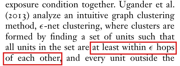
The rows Unit of Table 16.3 do not use the sampler. The estimand and the unbiasedness of the Horvitz–Thompson estimator with a correctly specified exposure mapping and the actual, positive exposure probabilities are unaffected. In my simulations under both samplers, the estimated standard deviation under cluster randomization is at most 0.70 of the unit-level value on every network. No printed entry is shown to be wrong. The sampler changes; if the package generated the rows Cluster, they have to be computed again before they are read as results for 3-net clustering. The printed definition of ϵ\epsilon-net clustering on the same page is the subject of P045-E010.

Corrected
Package, R/make_tr_vec_bernoulli.R, line 77, corrected. The same two lines replace line 123.
LineCode
77  remaining <- which(!marked)
  v_j <- remaining[sample.int(length(remaining), 1)]

For every finite undirected network, the loop then returns centers that are pairwise at least three hops apart, with every unit within two hops of a center. The treatment assignments have to be drawn again and the exposure probabilities recomputed under the corrected sampler.

Crop of Table 16.3 on page 305, 'Comparing unit to cluster randomization', with columns Randomization, Estimator, Estimand, True value, Average value, Bias, SD and RMSE, four rows and the note below the table. Red boxes mark the two Cluster rows (Horvitz-Thompson: 58.12, 57.52, minus 0.60, 61.31, 61.30; Hajek: 58.12, 55.01, minus 3.10, 28.89, 29.05) and the words 'Cluster = three-net clustering.' in the note.
Table 16.3, p. 305 (PDF p. 17). The marked rows are the two rows for cluster randomization, and the marked words of the note say that Cluster is three-net clustering.
A chart of two distributions of the number of clusters in one clustering of the 400 units. The horizontal axis runs from 45 to 200 clusters and the vertical axis gives the share of clusterings in percent, from 0 to 14. The blue distribution, the repaired sampler, is narrow: it lies between 48 and 72 clusters and peaks near 60 at about 14 percent; its mean is 60.4. The orange distribution, the package's sampler as written, peaks near 62 at about 4 percent and has a long right tail that passes 100 and 150 clusters; its mean is 83.8. A note says that 0.9 percent of the clusterings of the package's sampler have more than 200 clusters and that the largest has 326.
Number of clusters in one clustering of 400 units, for the package’s sampler as written (orange) and for the repaired sampler (blue): 50,000 clusterings per sampler, on five networks.

In the toy example every group has an arm with one unit, so the variance estimator for a direct effect that p. 310 describes is undefined; the two direct-effect variances in the output omit the undefined terms and are too small in expectation.

Section 16.5.1, toy example, p. 311 (PDF p. 23), the two direct-effect variances in the printed output; with the description of the variance estimators and of the design on p. 310 (PDF p. 22)

See also under Formal statements (Lean): P045-T3, P045-T4, P045-T26

As printed

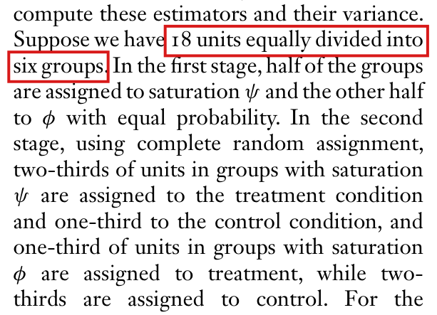
p. 310. When stratified interference holds, their proposed variance estimators are unbiased if unit causal effects are additive (e.g., yig(1,ψ)=yig(0,ψ)+dy_{ig}(1,\psi)=y_{ig}(0,\psi)+d, where dd is constant) and otherwise positively biased. … Suppose we have 18 units equally divided into six groups. In the first stage, half of the groups are assigned to saturation ψ\psi and the other half to ϕ\phi with equal probability. In the second stage, using complete random assignment, two-thirds of units in groups with saturation ψ\psi are assigned to the treatment condition and one-third to the control condition, and one-third of units in groups with saturation ϕ\phi are assigned to treatment, while two-thirds are assigned to control.

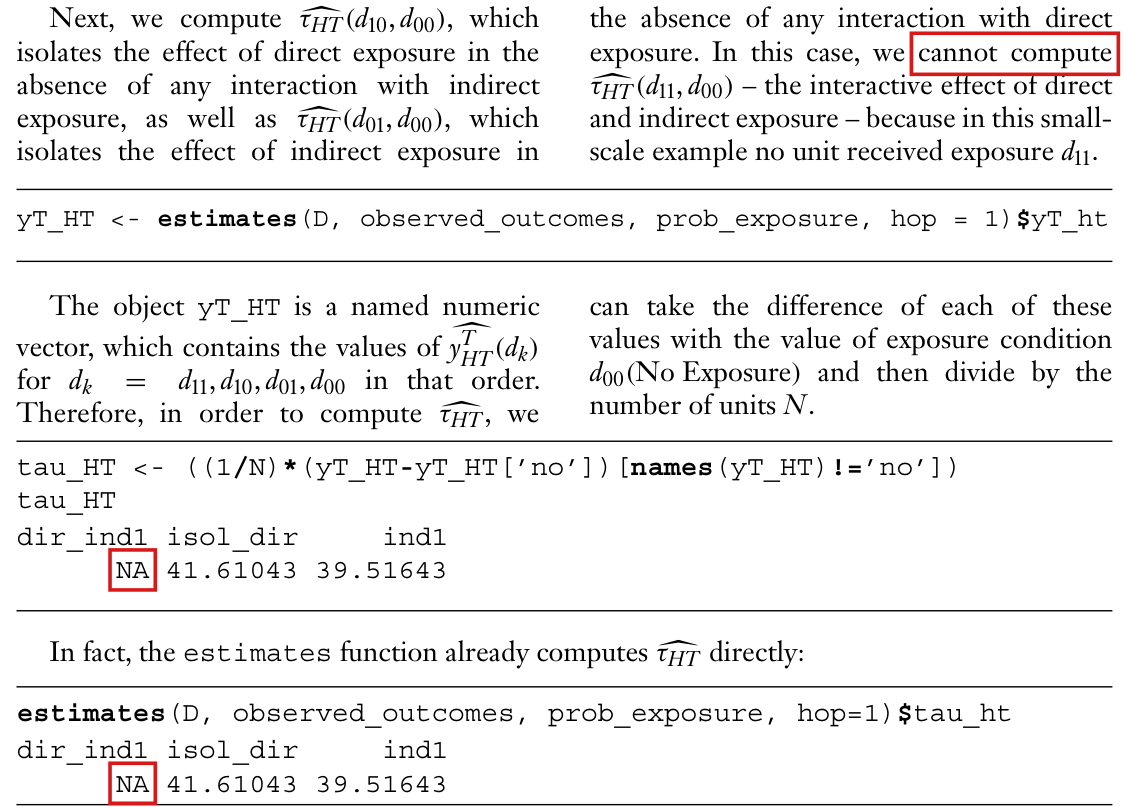
p. 311. The estimators and their variance are computed under the stratified interference assumption with the following function from the interference package: …

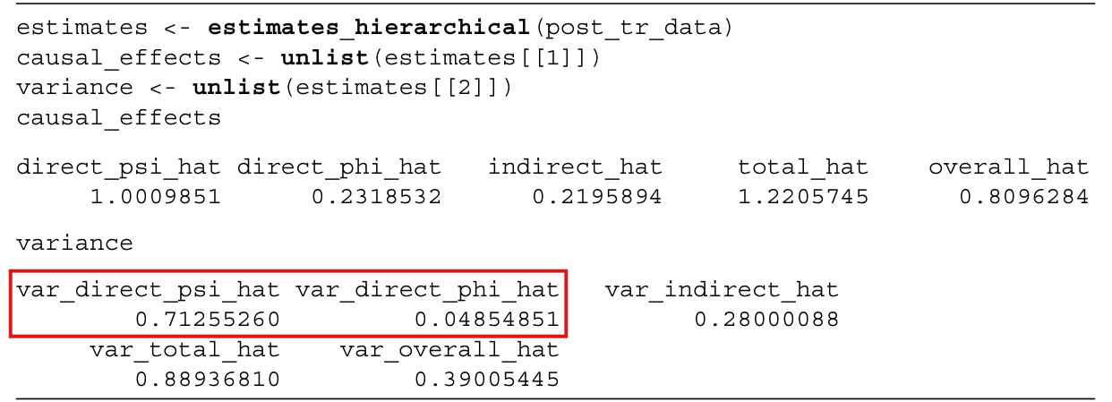
The variance output of estimates_hierarchical(post_tr_data) on p. 311, as printed.
EntryValue
var_direct_psi_hat0.71255260
var_direct_phi_hat0.04854851
var_indirect_hat0.28000088
var_total_hat0.88936810
var_overall_hat0.39005445
The problem

The variance estimator that Hudgens and Halloran (2008) propose for a direct effect, and that p. 310 describes, uses the sample variance of the observed outcomes in each arm of each group, and a sample variance needs at least two observations. In the toy design each group has three units, two in one arm and one in the other. One of the two sample variances is then undefined in every group. The function estimates_hierarchical sums the terms that are defined and drops the others without a warning. In each of the two direct-effect variances in the output, the part within groups therefore contains only the terms from the arms with two units. This quantity is not the estimator described, and it does not have the property stated on p. 310: in this design its expectation can fall below the true variance even with constant additive effects, and it does so under the outcome model of the example. The statement concerns the expectation over assignments and not the two printed numbers themselves. With other potential outcomes the omission can also bias the reported variance upward.

Evidence an exact counterexample

I checked the package output on data consistent with the example, an exact counterexample and a derivation of the bias.

The printed output. Data were found that match the six printed rows and all ten printed outputs to every printed digit. On these data both versions of estimates_hierarchical that I examined return the printed output with no warning. The six arms with one unit have undefined sample variance. The two direct-effect variances in the output are 0.695937+0.016616=0.7125530.695937+0.016616=0.712553 and 0.012457+0.036092=0.0485490.012457+0.036092=0.048549, where the first term is the part between groups and the second is the part within groups from the arms with two units.

The counterexample. In each of the six groups let the units have yig(0;s)=xiy_{ig}(0;s)=x_i and yig(1;s)=xi+1y_{ig}(1;s)=x_i+1 at both saturations ss, with (x1,x2,x3)=(1,2,3)(x_1,x_2,x_3)=(1,2,3). Unit effects are constant and additive with d=1d=1, and partial and stratified interference hold. The design has 20⋅36=14,58020\cdot 3^{6}=14{,}580 equally likely assignments. Summing over them in exact fractions, I obtain the following values.

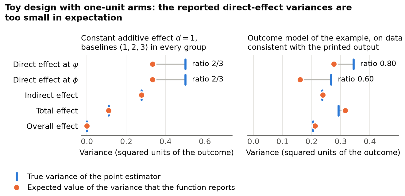
Constant additive effect d=1d=1, baseline outcomes (1,2,3)(1,2,3) in every group: true variance of each estimator and expected value of the reported variance.
EstimatorTrue varianceExpected reported variance
Direct effect at ψ\psi1/21/21/31/3
Direct effect at ϕ\phi1/21/21/31/3
Indirect effect5/185/185/185/18
Total effect1/91/91/91/9
Overall effect0000

The bias. Fix a saturation, and let GG be the number of groups. At the first stage, a fixed number of at least two groups is chosen uniformly for this saturation. The complete random assignments within groups at this saturation are independent across groups and independent of the first-stage selection. In group gg, with nn units of which mm are treated, let Sa,g2S^{2}_{a,g}, Sb,g2S^{2}_{b,g} and Sδ,g2S^{2}_{\delta,g} be the variances, with divisor n−1n-1, of the potential outcomes under treatment, of the potential outcomes under control and of the unit effects at this saturation. The difference in means in group gg has variance

Vg=Sa,g2m+Sb,g2n−m−Sδ,g2n.V_g=\frac{S^{2}_{a,g}}{m}+\frac{S^{2}_{b,g}}{n-m}-\frac{S^{2}_{\delta,g}}{n}.

If the within-group term of the variance estimator has expectation BgB_g in group gg, the estimator has bias G−2∑g(Bg−Vg)G^{-2}\sum_{g}(B_g-V_g). When both arms have at least two units, Bg=Sa,g2/m+Sb,g2/(n−m)B_g=S^{2}_{a,g}/m+S^{2}_{b,g}/(n-m), and the bias is G−2∑gSδ,g2/nG^{-2}\sum_{g}S^{2}_{\delta,g}/n. Under this design the bias is nonnegative, and it is zero exactly when unit effects are constant within every group; the constants may differ across groups. Otherwise it is positive. In the toy design G=6G=6 and n=3n=3, with m=2m=2 at ψ\psi and m=1m=1 at ϕ\phi. When the term of the arm with one unit is dropped, Bg=Sa,g2/2B_g=S^{2}_{a,g}/2 at ψ\psi and Bg=Sb,g2/2B_g=S^{2}_{b,g}/2 at ϕ\phi, and I obtain

Bias⁡ψ=1G2∑g=1G(Sδ,g23−Sb,g2),Bias⁡ϕ=1G2∑g=1G(Sδ,g23−Sa,g2).\operatorname{Bias}_{\psi}=\frac{1}{G^{2}}\sum_{g=1}^{G}\Bigl(\frac{S^{2}_{\delta,g}}{3}-S^{2}_{b,g}\Bigr), \qquad \operatorname{Bias}_{\phi}=\frac{1}{G^{2}}\sum_{g=1}^{G}\Bigl(\frac{S^{2}_{\delta,g}}{3}-S^{2}_{a,g}\Bigr).

Under constant effects Sδ,g2=0S^{2}_{\delta,g}=0; the bias at a saturation is negative if outcomes vary within any group at that saturation. Under the outcome model of the example, with Sx,g2S^{2}_{x,g} the variance of the baseline outcomes in group gg, the two biases are −(11/8) G−2∑gSx,g2-(11/8)\,G^{-2}\sum_{g}S^{2}_{x,g} and −(13/6) G−2∑gSx,g2-(13/6)\,G^{-2}\sum_{g}S^{2}_{x,g}. On the data consistent with the printed output, the expected reported variances are 0.2760.276 and 0.1610.161, and the true variances are 0.3440.344 and 0.2670.267; the ratios are 0.800.80 and 0.600.60. In the other direction, if yig(0;s)=0y_{ig}(0;s)=0 and yig(1;s)=xiy_{ig}(1;s)=x_i with (x1,x2,x3)=(1,2,3)(x_1,x_2,x_3)=(1,2,3) in every group, the expected reported variance at ψ\psi is 1/91/9 and the true variance is 1/181/18.

What survives

The five point estimates are unaffected, since an arm mean is defined for an arm with one unit. The variances of the indirect, total and overall effects use sample variances across the three groups at each saturation and are unaffected. Figure 16.6 shows point estimates only, in a design with 75 units per group and arms of 50 and 25. The direct-effect variance guarantee holds under stratified interference when a fixed number of at least two groups is selected uniformly for each saturation, the within-group complete random assignments at a fixed saturation are independent across groups and independent of the first-stage selection, and every arm has at least two units. Under these conditions the bias is zero exactly when unit effects are constant within each group, with possibly different constants across groups, and otherwise positive. What changes is the two direct-effect variances of the example and, for a user of the function, the variance reported for a direct effect in any design that has an arm with one unit.

Corrected

p. 310. Under stratified interference and the two-stage randomization specified here, the proposed variance estimator for a direct effect is unbiased exactly when unit causal effects are constant within each group; the constants may differ across groups. A common additive effect (e.g., yig(1,ψ)=yig(0,ψ)+dy_{ig}(1,\psi)=y_{ig}(0,\psi)+d, where dd is constant) is one such case. Otherwise its bias is positive. The first stage chooses a fixed number of groups uniformly for each saturation. For each fixed saturation, the complete random assignments within groups are independent across groups and independent of which groups are selected for that saturation. The variance estimator for a direct effect uses the sample variance of the outcomes in each arm of each group. It requires at least two treated and at least two control units in every group at that saturation, that is, 2≤Kg≤ng−22\le K_g\le n_g-2 where KgK_g is the number of treated units in group gg, and at least two groups at each saturation.

p. 311. The two direct-effect variances are not available in this design, because every group has an arm with one unit.

The variance output on p. 311, corrected.
EntryValue
var_direct_psi_hatNA
var_direct_phi_hatNA
var_indirect_hat0.28000088
var_total_hat0.88936810
var_overall_hat0.39005445

In the package, estimates_hierarchical should return NA with a warning when a sample variance that the formula needs is undefined. If numerical direct-effect variances are wanted in the example, use the uniform and independent randomization specified above with six groups of six units, treating four units per group at one saturation and two at the other. This keeps both saturations and has at least two units in every arm. The printed numbers would then change.

A block of R code and output in typewriter type. The first line reads 'estimates <- estimates_hierarchical(post_tr_data)'. The output lists five point estimates and then five variances. A red box marks the entries 'var_direct_psi_hat 0.71255260' and 'var_direct_phi_hat 0.04854851'. The other variances are var_indirect_hat 0.28000088, var_total_hat 0.88936810 and var_overall_hat 0.39005445.
Toy example, p. 311 (PDF p. 23): the call to estimates_hierarchical and its output, with the two direct-effect variance entries marked.
Twelve lines of text from the right column. Red boxes mark the words '18 units equally divided into' at the end of the second line and 'six groups' at the start of the third. The following lines say that two-thirds of units in groups with saturation psi are assigned to the treatment condition and one-third to the control condition, and one-third of units in groups with saturation phi are assigned to treatment.
Section 16.5.1, p. 310 (PDF p. 22), right column: the design of the toy example, with “18 units equally divided into six groups” marked. Each group has three units, two in one arm and one in the other.
Two panels, each with five rows and a horizontal axis of variance. Blue vertical ticks mark the true variance and orange dots the expected value of the reported variance. Left panel, constant additive effect: for the direct effects at psi and at phi the dot is at 0.33 and the tick at 0.50, labelled 'ratio 2/3'; for the indirect, total and overall effects the dot lies on the tick, at 0.28, 0.11 and 0. Right panel, outcome model of the example: for the direct effect at psi the dot is at 0.28 and the tick at 0.34, labelled 'ratio 0.80'; for the direct effect at phi the dot is at 0.16 and the tick at 0.27, labelled 'ratio 0.60'; for the indirect, total and overall effects the dot is at or slightly to the right of the tick, near 0.24, 0.30 and 0.21.
True variance of each point estimator and expected value of the variance that estimates_hierarchical reports, over the 14,580 assignments of the toy design. Left: every group has baseline outcomes (1,2,3)(1,2,3) and a constant additive effect d=1d=1. Right: the outcome model of the example, on data consistent with the printed output. The ratio is the expected reported variance divided by the true variance. The values are exact sums over the assignments.

Minor (10)

Real but inconsequential, for example a misprint that does not change a result.

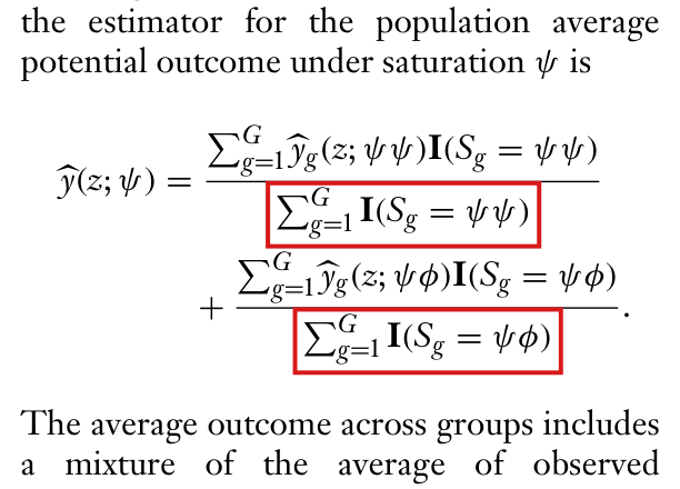
The pooled estimator y^(z;ψ)\widehat{y}(z;\psi) divides the sum of the group means by the number of all groups with saturation ψ\psi; the display prints the sum of two subgroup means, each with its own denominator.

Section 16.5.2, p. 312 (PDF p. 24), left column, the display after “the estimator for the population average potential outcome under saturation ψ\psi is”

See also under Formal statements (Lean): P045-T14, P045-T15

As printed

In other words, the estimator for the population average potential outcome under saturation ψ\psi is

y^(z;ψ)=∑g=1Gy^g(z;ψψ)I(Sg=ψψ)∑g=1GI(Sg=ψψ)+∑g=1Gy^g(z;ψϕ)I(Sg=ψϕ)∑g=1GI(Sg=ψϕ).\widehat{y}(z;\psi)=\frac{\sum_{g=1}^{G}\widehat{y}_g(z;\psi\psi)\mathbf{I}(S_g=\psi\psi)}{\colorbox{#ffe58a}{$\displaystyle \textstyle\sum_{g=1}^{G}\mathbf{I}(S_g=\psi\psi)$}}+\frac{\sum_{g=1}^{G}\widehat{y}_g(z;\psi\phi)\mathbf{I}(S_g=\psi\phi)}{\colorbox{#ffe58a}{$\displaystyle \textstyle\sum_{g=1}^{G}\mathbf{I}(S_g=\psi\phi)$}}.

The average outcome across groups includes a mixture of the average of observed outcomes for units with treatment zz in a group with realized saturation ψ\psi in a tract in which the realized saturation for the other group is ψ\psi, and the average of observed outcomes for units with treatment zz in a group with realized saturation ψ\psi in a tract in which the realized saturation for the other group is ϕ\phi.

The problem

On p. 310 the estimator y^(z;ψ)\widehat{y}(z;\psi) is the mean of the group means y^g(z;ψ)\widehat{y}_g(z;\psi) over all groups with saturation ψ\psi. Section 16.5.2 splits these groups by the saturation of the other group in the tract. Among the groups with saturation ψ\psi, let aa be the number of groups such that the other group in the tract has saturation ψ\psi, and let bb be the number such that it has saturation ϕ\phi. Let AA and BB be the sums of the group means over these two sets of groups. The estimator is (A+B)/(a+b)(A+B)/(a+b), which is the mixture of the subgroup means A/aA/a and B/bB/b with weights a/(a+b)a/(a+b) and b/(a+b)b/(a+b) that the next sentence describes. The display prints A/a+B/bA/a+B/b, the sum without weights. When both subgroups occur and the outcomes are positive, this exceeds the estimator; when one subgroup is empty, it contains 0/00/0, although the pooled estimator is still defined.

Evidence an exact counterexample

A derivation and an exact example. For positive aa and bb, I have

Aa+Bb−A+Ba+b=bAa(a+b)+aBb(a+b),\frac{A}{a}+\frac{B}{b}-\frac{A+B}{a+b}=\frac{bA}{a(a+b)}+\frac{aB}{b(a+b)},

which is positive when AA and BB are positive. For the example, I take the design of Section 16.5.2, with six groups of 75 units in three tracts, ψ=2/3\psi=2/3 and ϕ=1/3\phi=1/3. I let every baseline outcome be 11 and use the outcome multipliers of the package function make_dilated_out_hh_miss: in a group with saturation ψ\psi, a treated unit has outcome 9/49/4 and an untreated unit 11/811/8 when the other group in the tract has saturation ψ\psi, and 22 and 5/45/4 when it has saturation ϕ\phi. Let groups 1, 2 and 3 have saturation ψ\psi, with tracts (1,2)(1,2), (3,4)(3,4) and (5,6)(5,6), so that a=2a=2 and b=1b=1. For treated units the estimator is (9/2+2)/3=13/6(9/2+2)/3=13/6 and the display gives 9/4+2=17/49/4+2=17/4. For untreated units the values are 4/34/3 and 21/821/8. Of the 20 equally likely choices of the three groups with saturation ψ\psi, 8 place one such group in each tract. Then a=0a=0 and the first term of the display is 0/00/0. On all 20 choices the corrected form equals the estimator of p. 310, and the package function estimates_hierarchical computes that estimator.

What survives

The definition on p. 310, the sentence after the display and the argument of Section 16.5.2 are unaffected: pooling groups from tracts of different composition can bias the estimator of τD(ψψ)\tau^{D}(\psi\psi). The package computes the pooled estimator. The script for Figure 16.6 is not available, and it could not be confirmed that the figure was computed from the pooled estimator and not from the display.

Corrected

In other words, the estimator for the population average potential outcome under saturation ψ\psi is

y^(z;ψ)=∑g=1Gy^g(z;ψψ)I(Sg=ψψ)+∑g=1Gy^g(z;ψϕ)I(Sg=ψϕ)∑g=1GI(Sg=ψψ)+∑g=1GI(Sg=ψϕ),\widehat{y}(z;\psi)=\frac{\sum_{g=1}^{G}\widehat{y}_g(z;\psi\psi)\mathbf{I}(S_g=\psi\psi)+\sum_{g=1}^{G}\widehat{y}_g(z;\psi\phi)\mathbf{I}(S_g=\psi\phi)}{\colorbox{#ffe58a}{$\displaystyle \textstyle\sum_{g=1}^{G}\mathbf{I}(S_g=\psi\psi)+\sum_{g=1}^{G}\mathbf{I}(S_g=\psi\phi)$}},

which is defined whenever at least one group has saturation ψ\psi and each included group has at least one unit with treatment zz. Here Sg=ψψS_g=\psi\psi means that group gg has saturation ψ\psi and the other group in its tract has saturation ψ\psi, and Sg=ψϕS_g=\psi\phi means that group gg has saturation ψ\psi and the other group has saturation ϕ\phi. When both kinds of group occur, the estimator is the average of the two subgroup means weighted by the shares of the two kinds of group.

Two lines of text, a displayed formula in two lines, and two more lines of text. The formula sets y-hat(z; psi) equal to a fraction plus a second fraction. Red boxes mark the two denominators: the sum over g of the indicator of S_g = psi psi, and the sum over g of the indicator of S_g = psi phi.
Section 16.5.2, p. 312 (PDF p. 24), left column: the display for y^(z;ψ)\widehat{y}(z;\psi), with the two separate denominators marked.

An empty Horvitz–Thompson total is zero, and τHT^(d11,d00)\widehat{\tau_{HT}}(d_{11},d_{00}) in the example equals −13.27099-13.27099; the text says that it cannot be computed, and the package returns NA.

Section 16.4.2, p. 298 (PDF p. 10): the paragraph before the yT_HT code and the two printed outputs of τHT^\widehat{\tau_{HT}}; the function estimates of the interference package

See also under Formal statements (Lean): P045-T16, P045-T17

As printed

In this case, we cannot compute τHT^(d11,d00)\widehat{\tau_{HT}}(d_{11},d_{00}) – the interactive effect of direct and indirect exposure – because in this small-scale example no unit received exposure d11d_{11}.

Output printed twice on p. 298, after tau_HT and after the call to estimates.
dir_ind1isol_dirind1
NA41.6104339.51643
The problem

The chapter defines the Horvitz–Thompson total on p. 297 as a sum over all units,

yHTT^(dk)=∑i=1NI(Di=dk)Yiπi(dk),\widehat{y^T_{HT}}(d_k)=\sum_{i=1}^N\mathbf I(D_i=d_k)\frac{Y_i}{\pi_i(d_k)},

under the assumption that every unit has a positive probability of each exposure. When no unit receives d11d_{11}, every indicator in the sum is zero, and I call the total empty. An empty total equals 00, and the contrast τHT^(d11,d00)=−yHTT^(d00)/N\widehat{\tau_{HT}}(d_{11},d_{00})=-\widehat{y^T_{HT}}(d_{00})/N is a finite number. The sentence on p. 298 says that the contrast cannot be computed, and the package returns NA, because the function estimates replaces an empty total by NA. On such an assignment, the package does not compute the estimator of p. 297. The unbiasedness stated for that estimator refers to the mean over all assignments, with empty totals equal to zero. If the assignments on which the package returns NA are dropped, the mean of the remaining estimates can differ from the estimand. An empty Hajek ratio or sample mean is 0/00/0 and remains undefined.

Evidence an exact counterexample

The evidence is a derivation from the definition, a recalculation of the example with the package, and an exact counterexample.

Suppose that πi(d)>0\pi_i(d)>0 for every unit ii and that the observed outcomes are finite. If no unit has Di=dD_i=d, then every summand of yHTT^(d)\widehat{y^T_{HT}}(d) is 0⋅Yi/πi(d)=00\cdot Y_i/\pi_i(d)=0, and the total is 00. Since Yi=yi(d)Y_i=y_i(d) when Di=dD_i=d, I have

E[yHTT^(d)]=∑i=1Nyi(d) Pr⁡(Di=d)πi(d)=∑i=1Nyi(d),\mathbb E\bigl[\widehat{y^T_{HT}}(d)\bigr]=\sum_{i=1}^N y_i(d)\,\frac{\Pr(D_i=d)}{\pi_i(d)}=\sum_{i=1}^N y_i(d),

where the expectation is over all assignments, including those that place no unit in dd. In the last equality, I used that Pr⁡(Di=d)=πi(d)\Pr(D_i=d)=\pi_i(d).

For the example, I ran two versions of the package (commits a5b8dfb and c3fc7b3 of its repository) with the chapter’s seeds and the printed adjacency matrix, under the sampling algorithm that was the default before R 3.6.0. Both reproduce the printed assignment and the printed probabilities, and both return the totals (NA, 548.8142, 527.8742, 132.7099)(\texttt{NA},\,548.8142,\,527.8742,\,132.7099) for (d11,d10,d01,d00)(d_{11},d_{10},d_{01},d_{00}) and the printed contrasts. When I remove the line of estimates that sets an empty total to NA, the first total is 00 and the first contrast is (0−132.7099)/10=−13.27099(0-132.7099)/10=-13.27099. The other two contrasts do not change, and the Hajek contrast for d11d_{11} remains NA. The same line occurs in the package’s function for the full-neighbourhood exposures, which I did not test.

The counterexample uses the printed network of ten units, with two units assigned to treatment uniformly among the 45 pairs and potential outcomes

(yi(d11), yi(d10), yi(d01), yi(d00))=(2, 3/2, 5/4, 1)\bigl(y_i(d_{11}),\,y_i(d_{10}),\,y_i(d_{01}),\,y_i(d_{00})\bigr)=\bigl(2,\,3/2,\,5/4,\,1\bigr)

for every unit. The true total for d11d_{11} is 2020, and τ(d11,d00)=1\tau(d_{11},d_{00})=1. A unit with gig_i neighbours has πi(d11)=gi/45\pi_i(d_{11})=g_i/45, and every exposure probability of every unit is positive. The network has 20 edges. The 20 assignments that treat two adjacent units place those two units in d11d_{11}, and the other 25 assignments place no unit there. On the assignment that treats the adjacent units aa and bb, the total is 90(1/ga+1/gb)90(1/g_a+1/g_b), and the sum of these totals over the 20 edges is 900900. With empty totals equal to zero, I obtain

E[yHTT^(d11)]=90045=20,\mathbb E\bigl[\widehat{y^T_{HT}}(d_{11})\bigr]=\frac{900}{45}=20 ,

which is the true total. The mean over the 20 assignments with a unit in d11d_{11} is 900/20=45900/20=45. For the contrast, both d11d_{11} and d00d_{00} are received by some unit on 19 assignments. The mean of τHT^(d11,d00)\widehat{\tau_{HT}}(d_{11},d_{00}) over those 19 assignments is 1227/380≈3.231227/380\approx3.23. The mean over all 45 assignments, with empty totals equal to zero, is 11.

What survives

The definition of the estimator on p. 297, the estimand and the unbiasedness of the estimator with the true exposure probabilities are not affected. The contrasts 41.6104341.61043 and 39.5164339.51643 of the example stand, as does every Horvitz–Thompson output on an assignment in which each exposure involved is received by some unit. I could not determine whether the simulations with N=400N=400 are affected, because the scripts and draws behind their tables are not available and I do not know how they treated empty totals.

Corrected

In this case, no unit received exposure d11d_{11}. Since every π^i(d11)\widehat\pi_i(d_{11}) is positive, the total yHTT^(d11)\widehat{y^T_{HT}}(d_{11}) is zero, and τHT^(d11,d00)\widehat{\tau_{HT}}(d_{11},d_{00}) – the interactive effect of direct and indirect exposure – equals −yHTT^(d00)/N-\widehat{y^T_{HT}}(d_{00})/N.

Corrected output, in both places on p. 298.
dir_ind1isol_dirind1
−13.27099-13.2709941.6104339.51643

In general, let dkd_k be an exposure such that πi(dk)>0\pi_i(d_k)>0 for all units ii. Then

yHTT^(dk)=∑i=1NI(Di=dk)Yiπi(dk)\widehat{y^T_{HT}}(d_k)=\sum_{i=1}^N\mathbf I(D_i=d_k)\frac{Y_i}{\pi_i(d_k)}

is defined for every assignment, and it equals 00 when no unit has Di=dkD_i=d_k. If positive estimates π^i(dk)\widehat\pi_i(d_k) are used instead, replace πi(dk)\pi_i(d_k) by π^i(dk)\widehat\pi_i(d_k) in this formula; an empty total is still zero. With the true probabilities, its expectation over all assignments is ∑i=1Nyi(dk)\sum_{i=1}^N y_i(d_k). The Hajek estimator and the sample mean of an exposure that no unit receives remain undefined. In the package, the function estimates should keep the zero total and not replace it by NA.

Crop of the middle of page 298: two paragraphs set in two columns, a one-line sentence, three blocks of R code, and the output printed after two of them. Red boxes mark the words 'cannot compute' in the sentence about the estimate of tau HT of d11 and d00, and the entry NA under the column dir_ind1 in each of the two printed outputs, which otherwise read 41.61043 and 39.51643.
Section 16.4.2, p. 298 (PDF p. 10). The marked terms are the words “cannot compute” and the entry NA for dir_ind1 in each of the two printed outputs.

For i>1i>1, the vector z−i\mathbf z_{-i} begins with z1z_1, not with ziz_i.

Section 16.3, p. 292 (PDF p. 4), right column: the definition of z−i\mathbf z_{-i}

See also under Formal statements (Lean): P045-T18

As printed

For convenience, let z−i=(zi,…,zi−1,zi+1,…,zN)′\mathbf z_{-i}=(z_{\colorbox{#ffe58a}{$i$}},\ldots,z_{i-1},z_{i+1},\ldots,z_N)' denote the (N−1)(N-1)-element vector that removes the iith element from z\mathbf z.

The problem

The words define z−i\mathbf z_{-i} as the vector z\mathbf z with its iith element removed. The formula begins with ziz_i, the element that is removed. For i>1i>1, the correct first entry is z1z_1.

Evidence a check of the printed page

The evidence is a check of the page. The first subscript in the formula is the letter ii. The definition z=(z1,…,zN)′\mathbf z=(z_1,\ldots,z_N)' at the top of the same column has the numeral 11 in that place. For N=4N=4 and i=3i=3, removing the third element of (z1,z2,z3,z4)′(z_1,z_2,z_3,z_4)' leaves (z1,z2,z4)′(z_1,z_2,z_4)', and the printed formula begins with z3z_3 instead. The same page uses z−i\mathbf z_{-i} for “the treatment assignment of all other households”.

What survives

Nothing else changes. The words beside the formula give the intended definition, and the chapter uses z−i\mathbf z_{-i} in that sense afterwards.

Corrected

For convenience, let z−i=(z1,…,zi−1,zi+1,…,zN)′\mathbf z_{-i}=(z_{\colorbox{#ffe58a}{$1$}},\ldots,z_{i-1},z_{i+1},\ldots,z_N)' denote the (N−1)(N-1)-element vector that removes the iith element from z\mathbf z. For N>1N>1, the vector begins with z2z_2 when i=1i=1 and ends with zN−1z_{N-1} when i=Ni=N; for N=1N=1, it is empty.

Crop of nine lines from the right column of page 292. A red box marks the first entry of the displayed vector z sub minus i, which is printed as z sub i and is followed by dots, z sub i minus 1, z sub i plus 1, dots, z sub N.
Section 16.3, p. 292 (PDF p. 4), right column. The marked term is the first entry of the vector z−i\mathbf z_{-i}.

Under complete random assignment, a treated unit has ψng−1\psi n_g-1 treated group members other than itself, not ψ(ng−1)\psi(n_g-1).

Section 16.5.1, p. 310 (PDF p. 22), left column, first lines, the parenthesis beginning “(i.e.,”

See also under Formal statements (Lean): P045-T19

As printed

… complete random assignment, the individual-level direct effect for unit ii would contrast outcomes with different numbers of group members other than ii assigned to treatment (i.e., ψ(ng−1)\colorbox{#ffe58a}{$\psi(n_g-1)$} when ii is assigned to treatment and ψ(ng)\psi(n_g) when ii is assigned to control).

The problem

Complete random assignment at saturation ψ\psi treats exactly ψng\psi n_g of the ngn_g units in the group. If unit ii is treated, it is one of them, and ψng−1\psi n_g-1 of the other units are treated. If unit ii is in control, all ψng\psi n_g treated units are among the others. The printed ψ(ng−1)\psi(n_g-1) equals ψng−ψ\psi n_g-\psi, which exceeds the count for a treated unit by 1−ψ1-\psi.

Evidence a derivation

A derivation, and the example on the same page. When Zig=zZ_{ig}=z, the number of treated group members other than ii is

∑j≠iZjg=ψng−z.\sum_{j\neq i}Z_{jg}=\psi n_g-z .

In the toy example, ng=3n_g=3 and ψ=2/3\psi=2/3. Among the three assignments that treat two of the three units, a treated unit has one treated group member other than itself and a control unit has two. The printed expression equals 4/34/3 for the treated unit.

What survives

The point of the parenthesis is unaffected: under complete random assignment, the outcomes of a treated unit and of a control unit are compared at different numbers of treated group members. The count ψng\psi n_g for a control unit is correct, and nothing else in the chapter uses the expression.

Corrected

… complete random assignment, the individual-level direct effect for unit ii would contrast outcomes with different numbers of group members other than ii assigned to treatment (i.e., ψng−1\colorbox{#ffe58a}{$\psi n_g-1$} when ii is assigned to treatment and ψ(ng)\psi(n_g) when ii is assigned to control).

Seven lines of text from the top of the left column. A red box marks the expression 'psi (n_g minus 1)' in the parenthesis '(i.e., psi (n_g minus 1) when i is assigned to treatment and psi (n_g) when i is assigned to control)'.
Section 16.5.1, p. 310 (PDF p. 22), top of the left column: the parenthesis that counts the treated group members other than ii, with ψ(ng−1)\psi(n_g-1) marked.

The labels of the first two columns of Figure 16.6 are interchanged: the first column shows the direct effect at ψ\psi and the second shows the direct effect at ϕ\phi.

Figure 16.6, p. 312 (PDF p. 24), the labels above the first two columns

See also under Formal statements (Lean): P045-T24

As printed

Column labels, from left to right: τ^D(ϕ)\widehat{\tau}^{D}(\colorbox{#ffe58a}{$\phi$}), τ^D(ψ)\widehat{\tau}^{D}(\colorbox{#ffe58a}{$\psi$}), τ^I(ψ,ϕ)\widehat{\tau}^{I}(\psi,\phi), τ^To(ψ,ϕ)\widehat{\tau}^{To}(\psi,\phi), τ^O(ψ,ϕ)\widehat{\tau}^{O}(\psi,\phi). The caption ends: The dashed vertical line represents the value of the estimand.

The problem

Each dashed line marks the estimand of the estimator named above its column. In the bottom row, the outcome model on p. 310 gives τD(ψ)=(2−1.25) b=3b/4\tau^{D}(\psi)=(2-1.25)\,b=3b/4 and τD(ϕ)=(1.5−1) b=b/2\tau^{D}(\phi)=(1.5-1)\,b=b/2, where bb is the population mean of yig(0,ϕ)y_{ig}(0,\phi). The line for ϕ\phi should therefore stand at two-thirds of the line for ψ\psi. In the figure the line of the first column is at about 0.5950.595 and the line of the second is at about 0.3970.397, a ratio of 1.501.50. The two labels are in the reverse order. With the printed labels, each direct effect is attached to the wrong saturation, and so is the direction of its bias in the upper row.

Evidence a check of the printed page

A check of the page against the outcome model stated in the text. The positions of the ten dashed lines were measured from the drawing in the PDF. In the bottom row they are 0.5950.595, 0.3970.397, 0.1990.199, 0.7940.794 and 0.4630.463 from left to right. With b=0.794b=0.794, the position of the line for the total effect, these agree to within 0.0020.002 with 3b/43b/4, b/2b/2, b/4b/4, bb and 7b/127b/12, the values of τD(ψ)\tau^{D}(\psi), τD(ϕ)\tau^{D}(\phi), τI\tau^{I}, τTo\tau^{To} and τO\tau^{O} under the outcome model. In both rows the line for the total effect minus the line for the indirect effect agrees, within measurement precision, with the line of the first column, as the identity τTo=τD(ψ)+τI\tau^{To}=\tau^{D}(\psi)+\tau^{I} requires, and differs from the line of the second column by more than 0.10.1. The package also returns the direct effect at ψ\psi before the direct effect at ϕ\phi, which is the order of the output printed on p. 311. The simulation behind the figure was not run again, because its script and seeds are not available.

What survives

The histograms, the dashed lines and the other three columns are unchanged. So is the lesson of the figure, that the estimators are unbiased under partial interference and biased when interference crosses groups. Only the two labels change.

Corrected

Column labels, from left to right: τ^D(ψ)\widehat{\tau}^{D}(\colorbox{#ffe58a}{$\psi$}), τ^D(ϕ)\widehat{\tau}^{D}(\colorbox{#ffe58a}{$\phi$}), τ^I(ψ,ϕ)\widehat{\tau}^{I}(\psi,\phi), τ^To(ψ,ϕ)\widehat{\tau}^{To}(\psi,\phi), τ^O(ψ,ϕ)\widehat{\tau}^{O}(\psi,\phi).

A grid of ten histograms of point estimates, in five columns and two rows labelled 'General interference' and 'Partial interference', each with a dashed vertical line. Red boxes mark the labels above the first two columns, which read tau-hat D(phi) and tau-hat D(psi). In the bottom row the dashed line of the first column is near 0.6 and that of the second column is near 0.4. The caption below ends 'The dashed vertical line represents the value of the estimand.'
Figure 16.6, p. 312 (PDF p. 24), with its caption. The labels above the first two columns are marked: the first reads τ^D(ϕ)\widehat{\tau}^{D}(\phi) and the second reads τ^D(ψ)\widehat{\tau}^{D}(\psi).

In the expansion of μHT,None^(1)\widehat{\mu_{HT,None}}(\mathbf{1}) on p. 301, both denominators are πi=Pr⁡[Zi=1]\pi_i=\Pr[Z_i=1], not the exposure probabilities πi(d11)\pi_i(d_{11}) and πi(d10)\pi_i(d_{10}).

Section 16.4.3, p. 301 (PDF p. 13), left column, first display, second equality, and the sentence that begins “Therefore, the misspecified”

See also under Formal statements (Lean): P045-T12, P045-T13

As printed
μHT,None^(1)=1N∑i=1NI(Zi=1)Yiπi=1N∑i=1N(I(Di=d11)yi(d11)πi(d11)+I(Di=d10)yi(d10)πi(d10)),\begin{aligned} \widehat{\mu_{HT,None}}(\mathbf{1})&=\frac{1}{N}\sum_{i=1}^{N}\mathbf{I}(Z_i=1)\frac{Y_i}{\pi_i}\\ &=\frac{1}{N}\sum_{i=1}^{N}\left(\mathbf{I}(D_i=d_{11})\frac{y_i(d_{11})}{\colorbox{#ffe58a}{$\displaystyle \pi_i(d_{11})$}}+\mathbf{I}(D_i=d_{10})\frac{y_i(d_{10})}{\colorbox{#ffe58a}{$\displaystyle \pi_i(d_{10})$}}\right), \end{aligned}

“where πi=Pr⁡[Zi=1]\pi_i=\Pr[Z_i=1], while the unbiased estimator would be” μHT^(1)=μHT^(d11)\widehat{\mu_{HT}}(\mathbf{1})=\widehat{\mu_{HT}}(d_{11}) … “Therefore, the misspecified μHT,None^(1)\widehat{\mu_{HT,None}}(\mathbf{1}) is biased for μHT^(1)\widehat{\mu_{HT}}(\mathbf{1}) insofar as yi(d11)≠yi(d10)y_i(d_{11})\ne y_i(d_{10}) for some ii.”

The problem

The first line of the display defines the estimator that ignores interference. It weights the outcome of every treated unit by 1/πi1/\pi_i, where πi\pi_i is the probability that unit ii is treated. The second line is presented as an expansion of the first over the two exposure conditions of a treated unit, d11d_{11} (a treated direct peer) and d10d_{10} (none). Such an expansion keeps the denominator πi\pi_i in both terms. The printed line divides instead by the exposure probabilities πi(d11)\pi_i(d_{11}) and πi(d10)\pi_i(d_{10}), and the result is a different quantity. Its expectation is μ(d11)+μ(d10)\mu(d_{11})+\mu(d_{10}), the sum of the averages of two potential outcomes. The expectation of the first line is the mixture of yi(d11)y_i(d_{11}) and yi(d10)y_i(d_{10}) that the surrounding text describes. The closing sentence also calls the estimator biased for another estimator, μHT^(1)\widehat{\mu_{HT}}(\mathbf{1}), where the estimand μ(1)\mu(\mathbf{1}) is meant. The condition “for some ii” in that sentence is the subject of P045-E016.

Evidence an exact counterexample

The evidence is a derivation and an exact counterexample. For the derivation, suppose that the first-degree exposure mapping of p. 294 is correctly specified and that πi\pi_i, πi(d11)\pi_i(d_{11}) and πi(d10)\pi_i(d_{10}) are positive for every ii. By the definition of the exposure conditions, the events {Di=d11}\{D_i=d_{11}\} and {Di=d10}\{D_i=d_{10}\} partition the event {Zi=1}\{Z_i=1\}. This implies that πi=πi(d11)+πi(d10)\pi_i=\pi_i(d_{11})+\pi_i(d_{10}) and that I(Zi=1)=I(Di=d11)+I(Di=d10)\mathbf{I}(Z_i=1)=\mathbf{I}(D_i=d_{11})+\mathbf{I}(D_i=d_{10}). Since Yi=yi(d)Y_i=y_i(d) on the event {Di=d}\{D_i=d\}, I have

I(Zi=1) Yi=I(Di=d11) yi(d11)+I(Di=d10) yi(d10)\mathbf{I}(Z_i=1)\,Y_i=\mathbf{I}(D_i=d_{11})\,y_i(d_{11})+\mathbf{I}(D_i=d_{10})\,y_i(d_{10})

for every assignment. Dividing by πi\pi_i and averaging over ii gives the expansion in the corrected display below. The potential outcomes are fixed, and the two indicators have expectations πi(d11)\pi_i(d_{11}) and πi(d10)\pi_i(d_{10}). Taking expectations in the first line and in the printed second line, I obtain

E[μHT,None^(1)]=1N∑i=1N(πi(d11)πi yi(d11)+πi(d10)πi yi(d10)),E[printed second line]=1N∑i=1N(yi(d11)+yi(d10))=μ(d11)+μ(d10).\begin{aligned} \mathbb{E}\bigl[\widehat{\mu_{HT,None}}(\mathbf{1})\bigr]&=\frac{1}{N}\sum_{i=1}^{N}\left(\frac{\pi_i(d_{11})}{\pi_i}\,y_i(d_{11})+\frac{\pi_i(d_{10})}{\pi_i}\,y_i(d_{10})\right),\\ \mathbb{E}[\text{printed second line}]&=\frac{1}{N}\sum_{i=1}^{N}\bigl(y_i(d_{11})+y_i(d_{10})\bigr)=\mu(d_{11})+\mu(d_{10}). \end{aligned}

Note that in the first expectation the two weights of each unit sum to one. If every unit has a direct peer, then μ(1)=μ(d11)\mu(\mathbf{1})=\mu(d_{11}), and subtracting it from the first expectation gives the bias in the corrected sentence below.

For the counterexample, let ten units form a cycle, let exactly two units be treated, with all 45 assignments equally likely, and let yi(d11)=2y_i(d_{11})=2, yi(d10)=1y_i(d_{10})=1, yi(d01)=1y_i(d_{01})=1 and yi(d00)=0y_i(d_{00})=0 for every unit. Then πi=1/5\pi_i=1/5, πi(d11)=2/45\pi_i(d_{11})=2/45 and πi(d10)=7/45\pi_i(d_{10})=7/45. On each of the 10 assignments in which the two treated units are adjacent, the first line equals 22 and the printed second line equals 99. On each of the other 35 assignments, the first line equals 11 and the printed second line equals 9/79/7. Enumerating the 45 assignments in exact arithmetic, I find that the first line has expectation 11/911/9 and the printed second line has expectation 33, while μ(1)=2\mu(\mathbf{1})=2. The printed equality fails on all 45 assignments, and the corrected equality holds on all 45. The bias of the first line for μ(1)\mu(\mathbf{1}) is 11/9−2=−7/911/9-2=-7/9, which is the value of the corrected formula.

What survives

The definition of the estimator in the first line, the Horvitz–Thompson estimators of Section 16.4.2 and of the next display, and the explanation that the estimator mixes yi(d11)y_i(d_{11}) and yi(d10)y_i(d_{10}) are unaffected. In both copies of the package in the replication files, the corresponding code divides the treated total by one common probability. No error in Table 16.2 or in Figure 16.4 is established: they report simulations of Hajek estimators, and I found no dependence of them on the printed expansion. The second equality and the closing sentence change.

Corrected
μHT,None^(1)=1N∑i=1NI(Zi=1)Yiπi=1N∑i=1N(I(Di=d11)yi(d11)πi+I(Di=d10)yi(d10)πi),\begin{aligned} \widehat{\mu_{HT,None}}(\mathbf{1})&=\frac{1}{N}\sum_{i=1}^{N}\mathbf{I}(Z_i=1)\frac{Y_i}{\pi_i}\\ &=\frac{1}{N}\sum_{i=1}^{N}\left(\mathbf{I}(D_i=d_{11})\frac{y_i(d_{11})}{\colorbox{#ffe58a}{$\displaystyle \pi_i$}}+\mathbf{I}(D_i=d_{10})\frac{y_i(d_{10})}{\colorbox{#ffe58a}{$\displaystyle \pi_i$}}\right), \end{aligned}

where πi=Pr⁡[Zi=1]\pi_i=\Pr[Z_i=1]=πi(d11)+πi(d10){}=\pi_i(d_{11})+\pi_i(d_{10}). The equality holds for every assignment when the first-degree exposure mapping is correctly specified and πi>0\pi_i>0 for every ii. The closing sentence becomes: Therefore, relative to μ(1)\mu(\mathbf{1}), the misspecified μHT,None^(1)\widehat{\mu_{HT,None}}(\mathbf{1}) has bias

1N∑i=1Nπi(d10)πi {yi(d10)−yi(d11)}.\colorbox{#ffe58a}{$\displaystyle \frac{1}{N}\sum_{i=1}^{N}\frac{\pi_i(d_{10})}{\pi_i}\,\bigl\{y_i(d_{10})-y_i(d_{11})\bigr\}$}.

This formula for the bias holds when, in addition, every unit has at least one direct peer, so that μ(1)=μ(d11)\mu(\mathbf{1})=\mu(d_{11}).

Crop of the first display in the left column of page 301. The first line defines mu-hat HT,None of 1 as one over N times the sum over i of the indicator of Z_i = 1 times Y_i over pi_i. The second and third lines expand it as one over N times the sum of the indicator of D_i = d11 times y_i(d11) over pi_i(d11), plus the indicator of D_i = d10 times y_i(d10) over pi_i(d10). Below, the text reads 'where pi_i = Pr[Z_i = 1], while the unbiased estimator would be'. Red boxes mark the two denominators pi_i(d11) and pi_i(d10).
Section 16.4.3, p. 301 (PDF p. 13), left column, first display. The marked denominators are πi(d11)\pi_i(d_{11}) and πi(d10)\pi_i(d_{10}) in the second equality.

In the definition of ϵ\epsilon-net clustering, the units in the set are at least ϵ\epsilon hops apart, not “at least within ϵ\epsilon hops of each other”.

Section 16.4.6, p. 305 (PDF p. 17), last lines of the left column, continuing at the top of the right column

See also under Formal statements (Lean): P045-T20, P045-T21

As printed

Ugander et al. (2013) analyze an intuitive graph clustering method, ϵ\epsilon-net clustering, where clusters are formed by finding a set of units such that all units in the set are at least within ϵ\epsilon hops of each other, and every unit outside the set is within ϵ−1\epsilon-1 hops of a unit in the set.

The problem

The marked phrase joins two conditions that point in opposite directions. “At least” is a lower bound on the distance between two units in the set, and “within” is an upper bound. The definition needs the lower bound: any two units in the set are at least ϵ\epsilon hops apart, and the second clause supplies the upper bound, on the distance from a unit outside the set to the set. If the phrase is read as an upper bound, the two clauses can be impossible to satisfy together.

Evidence an exact counterexample

I checked the page and the intended greedy clustering procedure, and used an exact example.

The greedy procedure intended by make_tr_vec_bernoulli_cluster in the interference package picks an unmarked unit, marks every unit within two hops of it, and repeats until no unit is unmarked. These rules give pairwise separation of at least three hops and coverage within two hops. When only one eligible vertex remains, the actual sampler can choose an already-marked unit and violate the separation condition; see P045-E013. On a path with nine vertices and ϵ=3\epsilon=3, none of the 511 nonempty sets of vertices has all its members within three hops of each other and every vertex within two hops of the set, while 13 sets have all their members at least three hops apart and every vertex within two hops of the set. The article of Ugander et al. (2013) was not consulted.

What survives

The second clause of the definition and the intended 3-net design in Section 16.4.6 are unaffected by this wording correction. No change to the simulation numbers follows from this phrase alone.

Corrected

Ugander et al. (2013) analyze an intuitive graph clustering method, ϵ\epsilon-net clustering, where clusters are formed by finding a set of units such that all units in the set are at least ϵ\epsilon hops apart, and every unit outside the set is within ϵ−1\epsilon-1 hops of a unit in the set.

Six lines of text from the foot of the left column. Red boxes mark the words 'at least within epsilon hops' at the end of the fifth line and 'of each other' at the start of the sixth, in the sentence 'clusters are formed by finding a set of units such that all units in the set are at least within epsilon hops of each other, and every unit outside the'.
Section 16.4.6, p. 305 (PDF p. 17), foot of the left column: the definition of ϵ\epsilon-net clustering, with the phrase “at least within ϵ\epsilon hops of each other” marked. The sentence continues at the top of the right column.

Table 16.1 does not show that the variance estimator is consistent: at N=400N=400 the mean standard error is within 7.1 percent of the empirical standard deviation for two contrasts and exceeds it by 16.4 and 24.5 percent for the third.

Section 16.4.2, p. 299 (PDF p. 11), right column, last sentence; Table 16.1, p. 300 (PDF p. 12), columns SD and Mean SE

See also under Formal statements (Lean): P045-T22, P045-T23

As printed

“Moreover, the variance estimator is consistent, given that the mean of the standard error estimate approaches the empirical standard deviation from the simulation.”

The problem

The sentence infers that the variance estimator is consistent from the fact that, in Table 16.1, the mean of the standard error estimates is close to the empirical standard deviation of the point estimates. The conclusion does not follow from the table. Table 16.1 reports one design with N=400N=400, so it shows nothing about convergence as NN grows. The two columns also disagree for one of the three contrasts: for τ(d10,d00)\tau(d_{10},d_{00}) the mean standard error exceeds the empirical standard deviation by 24.5 percent for the Horvitz–Thompson estimator and by 16.4 percent for the Hajek estimator. Finally, agreement between the mean standard error and the standard deviation does not imply consistency, even if it holds at every sample size. The property that matters for a sampling distribution whose scale shrinks is that the ratio of the variance estimate to the true variance tends to one in probability, and the mean of the standard errors does not control that ratio. This finding concerns the inference in the sentence. It does not show that either variance estimator is inconsistent.

Evidence an exact counterexample

The evidence is a recalculation from Table 16.1 and an exact counterexample to the inference. The ratios of the printed entries are in the table below. For τ(d10,d00)\tau(d_{10},d_{00}) they are 33.11/26.60=473/38033.11/26.60=473/380 and 25.09/21.55=2509/215525.09/21.55=2509/2155, and both remain more than 16 percent above one when each entry is allowed to vary by its rounding error. The other four ratios are within 7.1 percent of one.

Table 16.1, p. 300: the mean standard error estimate against the empirical standard deviation.
EstimatorEstimandSDMean SEMean SE relative to SD
Horvitz–Thompsonτ(d11,d00)\tau(d_{11},d_{00})45.3245.94+1.4%+1.4\%
Horvitz–Thompsonτ(d10,d00)\tau(d_{10},d_{00})26.6033.11+24.5%+24.5\%
Horvitz–Thompsonτ(d01,d00)\tau(d_{01},d_{00})10.4510.33−1.1%-1.1\%
Hajekτ(d11,d00)\tau(d_{11},d_{00})36.6634.07−7.1%-7.1\%
Hajekτ(d10,d00)\tau(d_{10},d_{00})21.5525.09+16.4%+16.4\%
Hajekτ(d01,d00)\tau(d_{01},d_{00})8.388.41+0.4%+0.4\%

For the counterexample, let X1,…,XNX_1,\dots,X_N be independent signs, each equal to 11 or −1-1 with probability 1/21/2, and let TN=N−1∑i=1NXiT_N=N^{-1}\sum_{i=1}^N X_i estimate θ=0\theta=0. Then TNT_N is consistent and VN=Var⁡(TN)=1/NV_N=\operatorname{Var}(T_N)=1/N. Define B=1/2B=1/2 if X1=−1X_1=-1 and B=3/2B=3/2 if X1=1X_1=1, and define the variance estimate V^N=B2/N\widehat V_N=B^2/N. Since E[B]=1\mathbb{E}[B]=1, I have

E[V^N]=1N=VNfor every N,\mathbb{E}\Bigl[\sqrt{\widehat V_N}\Bigr]=\frac{1}{\sqrt N}=\sqrt{V_N}\qquad\text{for every } N,

so that the mean standard error equals the true standard deviation at every sample size. The estimate is also conservative in expectation, since E[V^N]=5/(4N)≥VN\mathbb{E}[\widehat V_N]=5/(4N)\ge V_N. But V^N/VN=B2\widehat V_N/V_N=B^2 takes the values 1/41/4 and 9/49/4 with probability 1/21/2 each. This implies that

Pr⁡( ∣V^N/VN−1∣>1/2 )=1for every N,\Pr\bigl(\,\bigl|\widehat V_N/V_N-1\bigr|>1/2\,\bigr)=1\qquad\text{for every } N,

and the ratio does not tend to one. Note that in this example the difference V^N−VN\widehat V_N-V_N does tend to zero, since ∣V^N−VN∣≤5/(4N)|\widehat V_N-V_N|\le 5/(4N). The counterexample concerns the inference only. It is not one of the chapter’s variance estimators.

What survives

All six rows of Table 16.1 stand, and so does the comparison that the table supports: the Hajek estimator has the smaller standard deviation and the smaller root-mean-square error for each contrast. No later result is derived from the sentence. Whether the two variance estimators are consistent under suitable asymptotic assumptions is not settled either way by this finding, and the large-NN confidence interval on p. 299 rests on separate theory.

Corrected

“At N=400N=400, the mean standard error estimates are within 7.1 percent of the empirical standard deviations for τ(d11,d00)\tau(d_{11},d_{00}) and τ(d01,d00)\tau(d_{01},d_{00}), and exceed them by 16.4 percent for Hajek and 24.5 percent for Horvitz–Thompson for τ(d10,d00)\tau(d_{10},d_{00}). These finite-sample comparisons do not establish asymptotic consistency.”

Crop of six lines from the right column of page 299. The text reads 'ance is with little cost in bias, as indicated by a smaller root-mean-square error. Moreover, the variance estimator is consistent, given that the mean of the standard error estimate approaches the empirical standard deviation from the simulation.' A red box marks the line 'the variance estimator is consistent, given'.
Section 16.4.2, p. 299 (PDF p. 11), right column, last sentence of the section. The marked line draws the conclusion of consistency.
Crop of Table 16.1 on page 300, 'Comparing Horvitz-Thompson to Hajek estimators using approximate exposure probabilities', with columns Estimator, Estimand, True value, Average value, Bias, SD, RMSE and Mean SE, six rows and the note below the table. Red boxes mark four entries in the two rows for tau(d10, d00): SD 26.60 and Mean SE 33.11 for Horvitz-Thompson, and SD 21.55 and Mean SE 25.09 for Hajek.
Table 16.1, p. 300 (PDF p. 12). The marked entries are the SD and the Mean SE for τ(d10,d00)\tau(d_{10},d_{00}), for the Horvitz–Thompson estimator and for the Hajek estimator.

The Progresa evaluation analyzed by Angelucci and De Giorgi (2009) randomized villages, not municipalities.

Section 16.5.3, p. 313 (PDF p. 25), right column, the sentences on Angelucci and De Giorgi (2009)

As printed

Similarly, Angelucci and De Giorgi (2009) analyze the indirect effects of the cash transfer program Progresa on consumption. In this case, only the first stage is randomized, assigning municipalities to treatment or control, while in the second stage a subset of individuals are offered treatment based on their income.

The problem

The unit of randomization is misnamed. In the cited study the randomization is at the level of the village (locality): of 506 rural villages, 320 were randomized in and 186 were randomized out. In the 2006 version of the study, municipalities appear in the description of the wider program, not as the unit that was randomized.

Evidence a check of the printed page

A check against the cited study. The abstract of the published article (American Economic Review 99(1): 486–508) says that the authors “use a village-level randomization”. The version of April 2006 (UCL Discussion Papers in Economics 06-01) states that “The randomization is conducted at the village level, with 186 villages randomized out”, and its Figure 1 shows 506 rural villages, 320 randomized in and 186 randomized out. The design section of the published article was not read, and the counts are those of the 2006 version.

What survives

The point of the example is unaffected: geographic groups are randomized in the first stage, and treatment within them follows eligibility by income. The chapter’s conclusion about what this design identifies does not depend on the name of the unit.

Corrected

Similarly, Angelucci and De Giorgi (2009) analyze the indirect effects of the cash transfer program Progresa on consumption. In this case, only the first stage is randomized, assigning villages (localities) to treatment or control, while in the second stage a subset of individuals are offered treatment based on their income.

Nine lines of text from the right column. A red box marks the word 'municipalities' in the sentence 'In this case, only the first stage is randomized, assigning municipalities to treatment or control, while in the second stage a subset of individuals are offered treatment based on their income.'
Section 16.5.3, p. 313 (PDF p. 25), right column: the description of the Progresa design, with “municipalities” marked.

The arXiv identifier in the reference to Taylor and Eckles (2017) is malformed: it has four digits after the point, and identifiers of September 2017 have five.

References, p. 319 (PDF p. 31), left column, the entry for Taylor and Eckles (2017)

As printed

Taylor, Sean J., and Dean Eckles. 2017. “Randomized Experiments to Detect and Estimate Social Influence in Networks.” arXiv:1709.0963v1 [cs.SI].

The problem

An arXiv identifier issued from January 2015 on has the form YYMM.NNNNN, with five digits after the point and an optional version suffix. The printed identifier has four digits after the point and is not a valid identifier.

Evidence a check of the printed page

I checked the printed identifier against arXiv’s identifier format. The chapter’s other identifiers of this period, 1809.09561 and 1711.06399, have five digits after the point. I then compared the authors, title, year and version with arXiv’s entry, which gives 1709.09636v1 [cs.SI]. I did not test whether the malformed string resolves on arXiv.

What survives

The authors, title and year identify the work, and the chapter’s discussion of it is unaffected.

Corrected

Taylor, Sean J., and Dean Eckles. 2017. “Randomized Experiments to Detect and Estimate Social Influence in Networks.” arXiv:1709.09636v1 [cs.SI].

Two entries of the reference list, four lines each. A red box marks 'arXiv:1709.0963v1' at the end of the third line of the entry 'Taylor, Sean J., and Dean Eckles. 2017. Randomized Experiments to Detect and Estimate Social Influence in Networks.' The next entry is Tchetgen and VanderWeele 2012.
References, p. 319 (PDF p. 31), left column: the entry for Taylor and Eckles (2017), with the arXiv identifier marked.

Clarity notes

Imprecise or ambiguous wording whose intended meaning is correct; not an error.

On p. 303, “the unbiased estimators” are the Hajek estimators whose exposure mapping is adequately specified; a Hajek estimator need not be exactly unbiased in a finite sample.

Section 16.4.3, p. 303 (PDF p. 15), left column, the paragraph that begins “Note that this example uses a relatively small set of units”

As printed

“Note that this example uses a relatively small set of units (N=400N=400), and the unbiased estimators (in this case, τH^(d11,d00)\widehat{\tau_H}(d_{11},d_{00}), τH^(d111,d000)\widehat{\tau_H}(d_{111},d_{000})) work with smaller subsets of the data than the coarser, biased estimators (here, τH^(d1,d0)\widehat{\tau_H}(d_1,d_0)).”

Intended meaning

The word separates the estimators whose exposure mapping allows for at least as much interference as the data-generating process from the coarser ones. The intended meaning is that the former carry no bias from the exposure mapping, and this is correct. The estimators named are Hajek estimators, which are ratios, and a ratio estimator need not be exactly unbiased in a finite sample. The chapter says so on p. 299, where the Hajek estimator “improves efficiency with a small cost in terms of finite-sample bias”. Table 16.2 reports biases of 1.29 and 0.85 for τH^(d11,d00)\widehat{\tau_H}(d_{11},d_{00}) when interference is of first degree, and of 4.28 and 2.58 for τH^(d111,d000)\widehat{\tau_H}(d_{111},d_{000}) when it is of second degree. An exact example confirms the point. Let exactly one of two units be treated, with assignment probabilities (1/4,3/4)(1/4,3/4), treated outcomes (1,3)(1,3), control outcomes zero and no interference. The Hajek contrast has expectation 5/25/2 and the Horvitz–Thompson contrast has expectation 22, which is the value of the estimand. The formulas and the simulation results are unchanged.

Corrected

“Note that this example uses a relatively small set of units (N=400N=400), and the estimators using adequately specified exposure mappings (in this case, τH^(d11,d00)\widehat{\tau_H}(d_{11},d_{00}), τH^(d111,d000)\widehat{\tau_H}(d_{111},d_{000})) work with smaller subsets of the data than the coarser, biased estimators (here, τH^(d1,d0)\widehat{\tau_H}(d_1,d_0)).”

Crop of seven lines from the left column of page 303. The text reads 'Note that this example uses a relatively small set of units (N = 400), and the unbiased estimators (in this case, tau-hat H of d11, d00, tau-hat H of d111, d000) work with smaller subsets of the data than the coarser, biased estimators (here, tau-hat H of d1, d0). This is apparent if one looks at the standard deviations in Table 16.2.' A red box marks the word 'unbiased'.
Section 16.4.3, p. 303 (PDF p. 15), left column. The marked word is “unbiased”.

The baseline outcome is a half-normal variable scaled by degree plus a normal term, as make_corr_out generates it; it is not an absolute standard normal variable.

Section 16.4.2, pp. 297–298 (PDF pp. 9–10), last paragraph of p. 297; see also p. 305 (PDF p. 17), right column

As printed

Specifically, we generate a variable with random values from an absolute standard normal distribution that is correlated with the unit’s first- and second-order degree – the number of peers and peers of peers, respectively (for which we use the arguments adj_matrix and make_corr_out in the function below). This variable determines the potential outcome under the d00d_{00} condition.

Intended meaning

The sentence describes a baseline outcome that is correlated with degree and is built by the function make_corr_out, which it names. That meaning is clear and correct. This function does not draw from the absolute value of a standard normal variable alone. It sets

yi(d00)=(ki+ki(2)+kiki(2)) ∣Xi∣+Ei,y_i(d_{00})=\bigl(k_i+k_i^{(2)}+k_ik_i^{(2)}\bigr)\,|X_i|+E_i,

where kik_i and ki(2)k_i^{(2)} are the first- and second-order degree of unit ii, and Xi∼N(0,1)X_i\sim N(0,1) and Ei∼N(1,0.252)E_i\sim N(1,0.25^2) are independent. This distribution has no lower bound, since EiE_i can be negative. The “positive lower bound” of the outcomes on p. 305 then refers to the smallest value in the fixed simulated population, which can be positive, and not to the distribution. The ten baseline values in the example of p. 298 are all positive, with minimum 6.1948786.194878. No reported result depends on the description.

Corrected

Specifically, we generate a variable (ki+ki(2)+kiki(2))∣Xi∣+Ei(k_i+k_i^{(2)}+k_ik_i^{(2)})|X_i|+E_i, where kik_i and ki(2)k_i^{(2)} are the unit’s first- and second-order degree – the number of peers and peers of peers, respectively – and Xi∼N(0,1)X_i\sim N(0,1) and Ei∼N(1,0.252)E_i\sim N(1,0.25^2) are independent. We use the arguments adj_matrix and make_corr_out in the function below. This variable determines the potential outcome under the d00d_{00} condition. A positive lower bound of the outcomes in a simulated population refers to its realized minimum, not a bound on this distribution.

Crop of six lines near the foot of the right column of page 297, beginning 'Specifically, we generate a variable with random values from'. Red boxes mark the phrase 'an absolute standard normal distribution', which runs over two lines.
Section 16.4.2, p. 297 (PDF p. 9), foot of the right column. The marked phrase describes the distribution of the baseline outcome.

Ω\Omega is the set of assignments that the design can produce; the count 2N2^N belongs to the full space {0,1}N\{0,1\}^N, on which the potential outcomes are defined.

Section 16.3, p. 292 (PDF p. 4), right column: the definition of Ω\Omega and the domain of the potential outcomes

As printed

Let Ω\Omega be the set of treatment assignment vectors z\mathbf z with ∣Ω∣=2N\colorbox{#ffe58a}{$|\Omega|=2^N$}. An experimental design is a plan for randomly selecting a particular value of z\mathbf z from the 2N2^N different possibilities with predetermined probability pzp_{\mathbf z} – for example, Bernoulli assignment (i.e., coin flips) or a completely randomized assignment strategy. Therefore, Ω={z:pz>0}\Omega=\{\mathbf z:p_{\mathbf z}>0\} and the realized treatment assignment Z=(Z1,…,ZN)′\mathbf Z=(Z_1,\ldots,Z_N)' is a random vector with support Ω\Omega and Pr⁡(Z=z)=pz\Pr(\mathbf Z=\mathbf z)=p_{\mathbf z}. For example, with a population of size N=10N=10 and an experimental design that randomly assigns without replacement a proportion p=0.2p=0.2 to treatment condition zi=1z_i=1 with uniform probability, there are (NpN)=45\binom{N}{pN}=45 possible treatment assignments (∣Ω∣=45|\Omega|=45) and the realized treatment assignment Z\mathbf Z has pz=145p_{\mathbf z}=\frac{1}{45}. … These potential outcomes are defined for each unit ii as the elements in the image of a function that maps assignment vectors to real valued outcomes, yi:Ω→Ry_i:\colorbox{#ffe58a}{$\Omega$}\to\mathbb R.

Intended meaning

The set Ω\Omega is the support of the design, {z:pz>0}\{\mathbf z:p_{\mathbf z}>0\}, and the chapter uses it in that sense. In the example on the same page, two of ten units are treated, and ∣Ω∣=(102)=45|\Omega|=\binom{10}{2}=45. The full space has 210=10242^{10}=1024 vectors. The count 2N2^N is the number of all vectors in {0,1}N\{0,1\}^N, and it equals ∣Ω∣|\Omega| only when the design gives every vector positive probability. With Ω\Omega as the support, the map yi:Ω→Ry_i:\Omega\to\mathbb R is defined only on the assignments that the design can produce. In the example these exclude the all-treated and all-control vectors, which define τ(1,0)\tau(\mathbf 1,\mathbf 0) on p. 300. The potential outcomes for such assignments are meant to exist, and their domain is {0,1}N\{0,1\}^N. No estimator or result depends on the count.

Corrected

There are 2N2^N treatment assignment vectors z\mathbf z in {0,1}N\{0,1\}^N. An experimental design is a plan for randomly selecting a particular value of z\mathbf z from the 2N2^N different possibilities with predetermined probability pzp_{\mathbf z} – for example, Bernoulli assignment (i.e., coin flips) or a completely randomized assignment strategy. Let Ω={z:pz>0}\Omega=\{\mathbf z:p_{\mathbf z}>0\} be the support of the design. The realized treatment assignment Z=(Z1,…,ZN)′\mathbf Z=(Z_1,\ldots,Z_N)' is a random vector with support Ω\Omega and Pr⁡(Z=z)=pz\Pr(\mathbf Z=\mathbf z)=p_{\mathbf z}. … These potential outcomes are defined for each unit ii as the elements in the image of a function that maps assignment vectors to real valued outcomes, yi:{0,1}N→Ry_i:\colorbox{#ffe58a}{$\{0,1\}^N$}\to\mathbb R.

Crop of the right column of page 292. Red boxes mark three terms: the equation that the size of Omega is 2 to the power N, the definition of Omega as the set of assignments z with positive probability p z, and, in the example with N equal to 10, the parenthesis stating that the size of Omega is 45.
Section 16.3, p. 292 (PDF p. 4), right column. The marked terms are the two descriptions of Ω\Omega and its size in the example with ten units.
Crop of eight lines from the right column of page 292, beginning 'To analyze the effect of different treatment assignments'. A red box marks the expression y i, colon, Omega, arrow, R, which defines the potential outcome as a function from Omega to the real numbers.
Section 16.3, p. 292 (PDF p. 4), right column, lower down. The marked term is the domain of the potential outcome function.

At N=400N=400 the greater variance of the finer exposure mappings often outweighs their reduction in squared bias; within the four rows of Table 16.2 that ignore interference, the squared bias exceeds the variance.

Section 16.4.3, p. 303 (PDF p. 15), left column, the sentence that begins “As such, with these sample sizes”; Table 16.2, p. 301 (PDF p. 13), the four rows with estimator τH^(d1,d0)\widehat{\tau_H}(d_1,d_0)

As printed

“This is apparent if one looks at the standard deviations in Table 16.2. As such, with these sample sizes, the root-mean-square error is swamped by estimation variance relative to bias. As NN gets larger, this would change: the standard deviation would get smaller, but the bias would remain.”

Intended meaning

The sentences before this one compare the finer exposure mappings, which use fewer units and have larger variance, with the coarser mapping, which has more bias. In that context the sentence says that, at N=400N=400, the variance added by a finer mapping often outweighs the squared bias that it removes. Table 16.2 supports this reading: the added variance exceeds the reduction in squared bias in seven of the eight comparisons between the estimator that ignores interference and a finer one. The exception is negative spillover with second-degree interference, where the first-degree estimator has the smaller root-mean-square error (22.21 against 27.54). Read as a statement about the two components of each root-mean-square error, the sentence does not hold for the four rows with estimator τH^(d1,d0)\widehat{\tau_H}(d_1,d_0). There the squared bias exceeds the squared standard deviation: 544.29 against 363.28, 1037.48 against 458.82, 221.12 against 216.97 and 572.17 against 186.32. Each of these inequalities survives the rounding of the printed entries. The entries of the table are unchanged.

Corrected

“With these sample sizes, the greater variance of finer exposure mappings often outweighs their reduction in squared bias when comparing root-mean-square errors.”

Crop of the last six lines of the left column of page 303. The text reads 'the data than the coarser, biased estimators (here, tau-hat H of d1, d0). This is apparent if one looks at the standard deviations in Table 16.2. As such, with these sample sizes, the root-mean-square error is swamped by estimation variance relative to bias. As N gets larger, this'. Red boxes mark the words 'swamped by estimation' and, on the next line, 'variance relative to bias.'
Section 16.4.3, p. 303 (PDF p. 15), left column, end of the column. The marked words are “swamped by estimation variance relative to bias”.
Crop of Table 16.2 on page 301, 'Misspecifying exposure conditions', with columns Spillover, Estimand, Estimator, True value, Bias, SD and RMSE and twelve rows. Red boxes mark the Bias and SD entries of the four rows whose estimator is tau-hat H of d1, d0: minus 23.33 and 19.06; minus 32.21 and 21.42; 14.87 and 14.73; 23.92 and 13.65.
Table 16.2, p. 301 (PDF p. 13). The marked entries are the Bias and the SD in the four rows with estimator τH^(d1,d0)\widehat{\tau_H}(d_1,d_0).

The estimator that ignores interference is biased when a weighted sum of the differences yi(d10)−yi(d11)y_i(d_{10})-y_i(d_{11}) is nonzero; a difference for some unit ii with πi(d10)>0\pi_i(d_{10})>0 suffices when all the differences have one sign, as they do in the chapter’s examples.

Section 16.4.3, p. 301 (PDF p. 13), left column, the sentence after the display for μHT^(1)\widehat{\mu_{HT}}(\mathbf{1})

See also under Formal statements (Lean): P045-T13

As printed

“Therefore, the misspecified μHT,None^(1)\widehat{\mu_{HT,None}}(\mathbf{1}) is biased for μHT^(1)\widehat{\mu_{HT}}(\mathbf{1}) insofar as yi(d11)≠yi(d10)y_i(d_{11})\ne y_i(d_{10}) for some ii.”

Intended meaning

The sentence explains that the estimator that ignores interference averages together the outcomes of treated units with and without a treated direct peer. In the chapter’s simulations with dilated effects, the differences yi(d10)−yi(d11)y_i(d_{10})-y_i(d_{11}) have one sign. In that setting a difference for some unit with πi(d10)>0\pi_i(d_{10})>0 gives a nonzero bias, and the statement is correct. As a general condition it is incomplete. For a correctly specified first-degree exposure mapping, positive treatment probabilities and at least one direct peer per unit, the bias relative to μ(1)\mu(\mathbf{1}) is the weighted sum N−1∑i[πi(d10)/πi]{yi(d10)−yi(d11)}N^{-1}\sum_{i}[\pi_i(d_{10})/\pi_i]\{y_i(d_{10})-y_i(d_{11})\}, and differences of opposite sign can cancel. For example, let two units be joined by one tie and be treated independently with probability 1/21/2, with y(d11)=(2,1)y(d_{11})=(2,1), y(d10)=(1,2)y(d_{10})=(1,2) and outcome zero for an untreated unit. The estimator takes the values 00, 22, 11 and 33 on the four assignments. Its expectation is 3/2=μ(1)3/2=\mu(\mathbf{1}), although yi(d11)≠yi(d10)y_i(d_{11})\ne y_i(d_{10}) for both units. The discussion of the simulations on p. 303 concerns spillovers of one sign and needs no change. The denominators of the display before this sentence are the subject of P045-E002.

Corrected

For a correctly specified first-degree exposure mapping, with πi=Pr⁡[Zi=1]>0\pi_i=\Pr[Z_i=1]>0 and at least one direct peer for every unit, the misspecified μHT,None^(1)\widehat{\mu_{HT,None}}(\mathbf{1}) has bias relative to μ(1)\mu(\mathbf{1})

1N∑i=1Nπi(d10)πi {yi(d10)−yi(d11)}.\colorbox{#ffe58a}{$\displaystyle \frac{1}{N}\sum_{i=1}^{N}\frac{\pi_i(d_{10})}{\pi_i}\,\bigl\{y_i(d_{10})-y_i(d_{11})\bigr\}$}.

This bias is nonzero when the differences yi(d10)−yi(d11)y_i(d_{10})-y_i(d_{11}) have one sign and at least one unit with πi(d10)>0\pi_i(d_{10})>0 has a nonzero difference, as in the examples considered here.

Crop of five lines from the left column of page 301. The text reads 'where pi_i(d11) = Pr[Z_i I(Z' theta_i > 0) = 1]. Therefore, the misspecified mu-hat HT,None of 1 is biased for mu-hat HT of 1 insofar as y_i(d11) is not equal to y_i(d10) for some i.' Red boxes mark the words 'insofar as y_i(d11) not equal to y_i(d10)' and, on the next line, 'for some i'.
Section 16.4.3, p. 301 (PDF p. 13), left column, the sentence after the display for μHT^(1)\widehat{\mu_{HT}}(\mathbf{1}). The marked words give the condition for bias.

For nominal coverage cc, the confidence interval on p. 299 uses the (1+c)/2(1+c)/2 quantile of the standard normal distribution; the printed subscript (1−α)/2(1-\alpha)/2 comes with no definition of α\alpha or of zz.

Section 16.4.2, p. 299 (PDF p. 11), left column, the confidence interval after “Confidence intervals are based on a large-NN normal approximation”

As printed

“Confidence intervals are based on a large-NN normal approximation:”

τHT^(dk,dl)±z(1−α)/2Var⁡^ [τHT^(dk,dl)].\widehat{\tau_{HT}}(d_k,d_l)\pm \colorbox{#ffe58a}{$\displaystyle z_{(1-\alpha)/2}$}\sqrt{\widehat{\operatorname{Var}}\,[\widehat{\tau_{HT}}(d_k,d_l)]}.

Intended meaning

The intended interval is the usual two-sided normal interval. The passage defines neither α\alpha nor zz, and the printed subscript is correct under one convention and wrong under the usual one. Let α\alpha be the error probability and let zq=Φ−1(q)z_q=\Phi^{-1}(q) be the qq-quantile of the standard normal distribution. Then the interval of level 1−α1-\alpha uses z1−α/2z_{1-\alpha/2}, and for α=0.05\alpha=0.05 the printed subscript gives Φ−1(0.475)=−0.063\Phi^{-1}(0.475)=-0.063 in place of Φ−1(0.975)=1.960\Phi^{-1}(0.975)=1.960. Suppose instead that α\alpha is the coverage and that zq=Φ−1(1−q)z_q=\Phi^{-1}(1-q) is the critical value for the upper tail. Then for α=0.95\alpha=0.95 the printed subscript gives Φ−1(0.975)=1.960\Phi^{-1}(0.975)=1.960, which is the correct value. A script distributed with the package computes its 95% intervals with qnorm(.975) and its 90% intervals with qnorm(.95), as the usual interval requires. No result of the chapter depends on the display.

Corrected

“Confidence intervals are based on a large-NN normal approximation: for nominal coverage cc,”

τHT^(dk,dl)±z(1+c)/2Var⁡^ [τHT^(dk,dl)],\widehat{\tau_{HT}}(d_k,d_l)\pm \colorbox{#ffe58a}{$\displaystyle z_{(1+c)/2}$}\sqrt{\widehat{\operatorname{Var}}\,[\widehat{\tau_{HT}}(d_k,d_l)]},

where zq=Φ−1(q)z_q=\Phi^{-1}(q) is the qq-quantile of the standard normal distribution. Equivalently, with error probability α=1−c\alpha=1-c, the critical value is z1−α/2z_{1-\alpha/2}.

Crop of seven lines from the left column of page 299. The text reads 'Confidence intervals are based on a large-N normal approximation:' and is followed by the interval tau-hat HT of d_k, d_l, plus or minus z with subscript (1 minus alpha) over 2, times the square root of the estimated variance of tau-hat HT. A red box marks z with its subscript (1 minus alpha)/2.
Section 16.4.2, p. 299 (PDF p. 11), left column. The marked term is the critical value z(1−α)/2z_{(1-\alpha)/2} in the confidence interval.

The columns of the printed output are adjusted Monte Carlo estimates of the exposure probabilities, (Cik+1)/(R+1)(C_{ik}+1)/(R+1), and each column sums to 34/3134/31 before rounding.

Section 16.4.1, p. 297 (PDF p. 9), first sentence of the page, on the output of make_prob_exposure_cond printed on p. 296 (PDF p. 8)

As printed

The columns capture πi\colorbox{#ffe58a}{$\boldsymbol{\pi}_i$}, the expected proportion of treatment assignments that result in each exposure.

Intended meaning

Each column of the output on p. 296 holds estimates π^i\widehat{\boldsymbol{\pi}}_i of the four exposure probabilities of one unit, computed from the R=30R=30 sampled assignments. Page 296 says that the example works with 30 random draws from Ω\Omega, and pp. 297–298 distinguish the estimates π^i(dk)\widehat\pi_i(d_k) from the true values πi(dk)\pi_i(d_k), so that this meaning is clear and correct. The chapter does not say that the package adds one to each count and to the number of draws. The entry for unit ii and exposure dkd_k is (Cik+1)/(R+1)(C_{ik}+1)/(R+1), where CikC_{ik} is the number of sampled assignments that place unit ii in dkd_k. Since the four counts of a unit sum to RR, I find that each column sums to (R+4)/(R+1)=34/31(R+4)/(R+1)=34/31 before rounding, and not to one. For unit 1 the unrounded entries are (3,6,13,12)/31(3,6,13,12)/31, the sample proportions are (2,5,12,11)/30(2,5,12,11)/30, and the exact probabilities over the 45 assignments are (3,6,21,15)/45(3,6,21,15)/45. The contrast 41.6104341.61043 on p. 298 is reproduced from these estimates, and no reported number changes.

Corrected

The columns contain adjusted Monte Carlo estimates π^i\widehat{\boldsymbol{\pi}}_i of each unit’s exposure probabilities: the entry for exposure dkd_k is (Cik+1)/(R+1)(C_{ik}+1)/(R+1), where CikC_{ik} is the number of the RR sampled assignments that place unit ii in dkd_k. The four entries of a column sum to (R+4)/(R+1)(R+4)/(R+1), here 34/3134/31, and not to one.

Crop of the first five lines of the left column of page 297, beginning 'The columns capture pi i, the expected proportion of treatment assignments that result in each exposure'. A red box marks the bold symbol pi sub i.
Section 16.4.1, p. 297 (PDF p. 9), first lines of the left column. The marked symbol is πi\boldsymbol{\pi}_i.

The guarantee is exact with true marginal and joint exposure probabilities. The context clearly treats Monte Carlo probabilities as numerical approximations; the guarantee should state this scope explicitly.

Section 16.4.2, last paragraph of p. 298 (PDF p. 10): the sentence that begins “These are conservative approximations” on the last line of the left column and continues in the right column; and the sentence “Both of these corrections …” at the top of p. 299 (PDF p. 11)

Classification before my review (the classification when the audit was first completed, before I reviewed it): Error, Moderate (entry P045-N016).

See also under Formal statements (Lean): P045-T32, P045-T33

My comment on this entry

As printed

The estimator τ^HT(dk,dl)\widehat{\tau}_{HT}(d_k,d_l) is unbiased when it is estimated with πi(dk)\pi_i(d_k) rather than π^i(dk)\widehat{\pi}_i(d_k). As mentioned above, when estimated with the latter, the estimator is not unbiased, but the bias becomes negligible with a sufficiently large number of replicates RR. We implement variance estimators for Var⁡[yT^HT(dk)]\operatorname{Var}\bigl[\widehat{y^T}_{HT}(d_k)\bigr] and Var⁡ [τ^HT(dk,dl)]\operatorname{Var}\,[\widehat{\tau}_{HT}(d_k,d_l)] as derived in equation 11 of Aronow and Samii (2017). These are conservative approximations of the exact variances that are guaranteed to have nonnegative bias relative to the variance of the randomization distribution of the estimators. Because unbiased estimators for Var⁡[yT^HT(dk)]\operatorname{Var}\bigl[\widehat{y^T}_{HT}(d_k)\bigr] are only identified when the joint exposure probabilities of every pair of units are positive, it is necessary to add a correction term to Var⁡^[yT^HT(dk)]\widehat{\operatorname{Var}}\bigl[\widehat{y^T}_{HT}(d_k)\bigr]. Second, because the Cov⁡[yT^HT(dk),yT^HT(dl)]\operatorname{Cov}\bigl[\widehat{y^T}_{HT}(d_k),\widehat{y^T}_{HT}(d_l)\bigr] is always unidentified, we use an approximation. Both of these corrections contribute to the nonnegative bias of the variance estimator.

Intended meaning

A variance estimator has nonnegative bias if its expectation over the randomization is at least the variance that it estimates. The guarantee holds when the variance estimators are computed with the exact marginal and joint exposure probabilities of the design and every unit has positive probability of the exposures concerned. This is the natural intended meaning. Page 294 explains that Monte Carlo probabilities approximate the exact probabilities with arbitrary precision and discusses keeping their bias small. Immediately before the guarantee on p. 298, the chapter distinguishes πi(dk)\pi_i(d_k) from π^i(dk)\widehat\pi_i(d_k) and says that the point estimator’s finite-RR bias becomes negligible with sufficiently many replicates. Read together, these passages describe the exact-probability result and an accurate numerical approximation to it.

The examples do use simulated exposure probabilities: 30 assignments drawn without replacement from 45 in the running example (p. 296), and R=10,000R=10{,}000 assignments in Section 16.4.2 (p. 299). Page 297 says that the estimates replace the true probabilities. These finite calculations need not preserve an exact sign guarantee. The example below shows that the expected variance estimate can be below the variance of the contrast computed with those same simulated probabilities. It does not test the numerical accuracy of the chapter’s R=10,000R=10{,}000 calculations.

The distinction follows from the expectation of a product of exposure indicators, which is the exact joint exposure probability. With that probability in the denominator of a positive-joint-probability term, the two cancel. A simulated denominator does not give this cancellation. The corrections for zero joint probabilities control the missing outcome products, not the Monte Carlo error. Adding the exact-probability restriction to the guarantee and to the following sentence about the corrections would make their intended scope explicit. The related qualification for the chapter “Estimating Causal Effects in Experiments with Network Spillovers” is listed as P044-N005.

The evidence is an exact counterexample, a check of the counterexample against the package, and a derivation for exact exposure probabilities.

The counterexample. Twelve units form three disjoint cliques of four: two distinct units are adjacent exactly when they belong to the same clique. Two units are treated, and the 66 assignments are equally likely. The exposure mapping is the chapter’s. A unit has exposure d11d_{11} if it and a neighbor are treated, d10d_{10} if it is treated and no neighbor is, d01d_{01} if it is untreated and a neighbor is treated, and d00d_{00} otherwise. Every potential outcome equals 1, so that the exposure mapping fully characterizes interference and τ(d01,d00)=0\tau(d_{01},d_{00})=0. For every unit, the exact probabilities of d11d_{11}, d10d_{10}, d01d_{01} and d00d_{00} are 3/663/66, 8/668/66, 27/6627/66 and 28/6628/66. The exposure probabilities are simulated from a sample of R=65R=65 distinct assignments, drawn uniformly without replacement from the 66 and independently of the realized assignment. The example on p. 296 also draws its 30 assignments without replacement, from 45. There are 66 such samples, one for each omitted assignment.

Fix two exposures, and let cijc_{ij} be the number of sampled assignments under which unit ii has the first exposure and unit jj has the second. The package estimates the joint probability by (cij+1{i=j})/(R+1)(c_{ij}+\mathbf{1}\{i=j\})/(R+1) when the two exposures are the same and by cij/Rc_{ij}/R when they differ. The marginal estimates are the diagonal entries in the first case (see P045-N001). In the counterexample the simulated probability of d01d_{01} is 27/6627/66 for a unit that has exposure d01d_{01} under the omitted assignment and 28/6628/66 for the other units. The simulated probability of d00d_{00} is 28/6628/66 for a unit that has exposure d00d_{00} under the omitted assignment and 29/6629/66 for the other units. For the two contrasted exposures, a simulated joint probability is zero exactly when the exact joint probability is zero. The failure does not come from a pair of exposures that is possible but absent from the sample.

I enumerated the 66×66=435666\times 66=4356 pairs of a sample and a realized assignment in exact rational arithmetic. For each pair I computed τ^HT(d01,d00)\widehat{\tau}_{HT}(d_{01},d_{00}) and the variance estimator displayed below, with the simulated probabilities in place of the exact ones.

The counterexample. Mean and Variance: of τ^HT(d01,d00)\widehat{\tau}_{HT}(d_{01},d_{00}). Expectation: of its variance estimator. Bias: the expectation minus the variance. In the first row the 66 samples are equally likely. In the second and third rows the sample is fixed, and the assignment that it omits treats two units of one clique or one unit in each of two cliques. The decimals are exact fractions rounded to six places.
Exposure probabilitiesSamplesMeanVarianceExpectationBias
Simulated, all samples66−67/53592-67/535920.4876580.447098−0.040560-0.040560
Simulated, one clique18−89/4872-89/48720.4872670.421232−0.066035-0.066035
Simulated, two cliques4825/487225/48720.4876550.456797−0.030858-0.030858
Exact000.5081040.50810400

In the first row the moments are over the sample and the realized assignment, and the exact values are

Var⁡ [τ^HT(d01,d00)]=113448938731232640299584,E[Var⁡^ [τ^HT(d01,d00)]]=10401294764232326402995840.\operatorname{Var}\,[\widehat{\tau}_{HT}(d_{01},d_{00})]=\frac{113448938731}{232640299584}, \qquad \mathbb{E}\Bigl[\widehat{\operatorname{Var}}\,[\widehat{\tau}_{HT}(d_{01},d_{00})]\Bigr]=\frac{1040129476423}{2326402995840}.

Their difference is −953130413/23499020160-953130413/23499020160, and the expectation is about 8.3 percent below the variance. In the second and third rows the moments are over the realized assignment. The bias is negative for each of the 66 samples. With the exact probabilities in the same formulas, the variance and the expectation of the variance estimator both equal 6050/119076050/11907.

The package. I ran the unchanged functions of two versions of the interference package (commits a5b8dfb and c3fc7b3) for the exposure mapping, the exposure probabilities, the variance and the covariance. For each of the 4356 pairs, I compared two quantities with the enumeration: the contrast computed with the package’s simulated probabilities, and the variance estimate that the package returns. In both versions they agree up to floating-point rounding.

Derivation for exact exposure probabilities. Let πi(d)=Pr⁡(Di=d)\pi_i(d)=\Pr(D_i=d) and πij(d,d′)=Pr⁡(Di=d, Dj=d′)\pi_{ij}(d,d')=\Pr(D_i=d,\,D_j=d'), with πii(d,d)=πi(d)\pi_{ii}(d,d)=\pi_i(d), and write Ii(d)=1{Di=d}I_i(d)=\mathbf{1}\{D_i=d\}. Let W^k\widehat W_k denote the variance estimator Var⁡^[yT^HT(dk)]\widehat{\operatorname{Var}}\bigl[\widehat{y^T}_{HT}(d_k)\bigr] and C^kl\widehat C_{kl} the estimator of Cov⁡[yT^HT(dk),yT^HT(dl)]\operatorname{Cov}\bigl[\widehat{y^T}_{HT}(d_k),\widehat{y^T}_{HT}(d_l)\bigr]. The package computes

W^k=∑i,j: πij(dk,dk)>0Ii(dk) Ij(dk) πij(dk,dk)−πi(dk)πj(dk)πij(dk,dk) YiYjπi(dk)πj(dk)+∑i≠j: πij(dk,dk)=0(Ii(dk) Yi22πi(dk)+Ij(dk) Yj22πj(dk)),C^kl=∑i,j: πij(dk,dl)>0Ii(dk) Ij(dl) πij(dk,dl)−πi(dk)πj(dl)πij(dk,dl) YiYjπi(dk)πj(dl)−∑i,j: πij(dk,dl)=0(Ii(dk) Yi22πi(dk)+Ij(dl) Yj22πj(dl)),\begin{aligned} \widehat W_k={}&\sum_{i,j:\,\pi_{ij}(d_k,d_k)>0}I_i(d_k)\,I_j(d_k)\,\frac{\pi_{ij}(d_k,d_k)-\pi_i(d_k)\pi_j(d_k)}{\pi_{ij}(d_k,d_k)}\,\frac{Y_iY_j}{\pi_i(d_k)\pi_j(d_k)}\\ &+\sum_{i\neq j:\,\pi_{ij}(d_k,d_k)=0}\Bigl(\frac{I_i(d_k)\,Y_i^2}{2\pi_i(d_k)}+\frac{I_j(d_k)\,Y_j^2}{2\pi_j(d_k)}\Bigr),\\ \widehat C_{kl}={}&\sum_{i,j:\,\pi_{ij}(d_k,d_l)>0}I_i(d_k)\,I_j(d_l)\,\frac{\pi_{ij}(d_k,d_l)-\pi_i(d_k)\pi_j(d_l)}{\pi_{ij}(d_k,d_l)}\,\frac{Y_iY_j}{\pi_i(d_k)\pi_j(d_l)}\\ &-\sum_{i,j:\,\pi_{ij}(d_k,d_l)=0}\Bigl(\frac{I_i(d_k)\,Y_i^2}{2\pi_i(d_k)}+\frac{I_j(d_l)\,Y_j^2}{2\pi_j(d_l)}\Bigr), \end{aligned}

and Var⁡^ [τ^HT(dk,dl)]=N−2(W^k+W^l−2 C^kl)\widehat{\operatorname{Var}}\,[\widehat{\tau}_{HT}(d_k,d_l)]=N^{-2}\bigl(\widehat W_k+\widehat W_l-2\,\widehat C_{kl}\bigr). The sums are over ordered pairs of units. The pairs with i=ji=j belong to the first sum of W^k\widehat W_k and to the second sum of C^kl\widehat C_{kl}.

Suppose that the probabilities are exact and that πi(dk)>0\pi_i(d_k)>0 and πi(dl)>0\pi_i(d_l)>0 for every unit ii. Since E[Ii(d) Ij(d′)]=πij(d,d′)\mathbb{E}\bigl[I_i(d)\,I_j(d')\bigr]=\pi_{ij}(d,d'), each term of a sum over positive joint probabilities has expectation equal to the corresponding term of Var⁡[yT^HT(dk)]\operatorname{Var}\bigl[\widehat{y^T}_{HT}(d_k)\bigr] or of the covariance. For a pair with πij(dk,dk)=0\pi_{ij}(d_k,d_k)=0, the term of the variance is −yi(dk) yj(dk)-y_i(d_k)\,y_j(d_k), and the second sum of W^k\widehat W_k has expectation (yi(dk)2+yj(dk)2)/2\bigl(y_i(d_k)^2+y_j(d_k)^2\bigr)/2 for that pair. For a pair with πij(dk,dl)=0\pi_{ij}(d_k,d_l)=0, the term of the covariance is −yi(dk) yj(dl)-y_i(d_k)\,y_j(d_l), and the second sum of C^kl\widehat C_{kl} has expectation −(yi(dk)2+yj(dl)2)/2-\bigl(y_i(d_k)^2+y_j(d_l)^2\bigr)/2. Collecting terms, I obtain

E[W^k]−Var⁡[yT^HT(dk)]=12∑i≠j: πij(dk,dk)=0(yi(dk)+yj(dk))2  ≥  0\mathbb{E}\bigl[\widehat W_k\bigr]-\operatorname{Var}\bigl[\widehat{y^T}_{HT}(d_k)\bigr]=\frac{1}{2}\sum_{i\neq j:\,\pi_{ij}(d_k,d_k)=0}\bigl(y_i(d_k)+y_j(d_k)\bigr)^2\;\ge\;0

and

E[Var⁡^ [τ^HT(dk,dl)]]−Var⁡ [τ^HT(dk,dl)]=12N2∑i≠j: πij(dk,dk)=0(yi(dk)+yj(dk))2+12N2∑i≠j: πij(dl,dl)=0(yi(dl)+yj(dl))2+1N2∑i,j: πij(dk,dl)=0(yi(dk)−yj(dl))2  ≥  0.\begin{aligned} \mathbb{E}\Bigl[\widehat{\operatorname{Var}}\,[\widehat{\tau}_{HT}(d_k,d_l)]\Bigr]-\operatorname{Var}\,[\widehat{\tau}_{HT}(d_k,d_l)]={}&\frac{1}{2N^2}\sum_{i\neq j:\,\pi_{ij}(d_k,d_k)=0}\bigl(y_i(d_k)+y_j(d_k)\bigr)^2\\ &+\frac{1}{2N^2}\sum_{i\neq j:\,\pi_{ij}(d_l,d_l)=0}\bigl(y_i(d_l)+y_j(d_l)\bigr)^2\\ &+\frac{1}{N^2}\sum_{i,j:\,\pi_{ij}(d_k,d_l)=0}\bigl(y_i(d_k)-y_j(d_l)\bigr)^2\;\ge\;0. \end{aligned}

In the counterexample no two units have joint probability zero of d01d_{01} or of d00d_{00}, and every difference yi(d01)−yj(d00)y_i(d_{01})-y_j(d_{00}) is zero. The last display then implies that the bias with exact probabilities is zero, in agreement with the last row of the table. In the first step of the derivation, I used that the probabilities inside the variance estimator are those of the distribution of the realized assignment. With simulated probabilities, the expectation of Ii(d) Ij(d′)I_i(d)\,I_j(d') is still the exact joint probability, the denominator is the simulated one, and the identities do not hold.

The exact-probability result, exposure mapping, estimands and statement about the point estimator’s bias are unaffected. The counterexample concerns the Horvitz–Thompson variance estimator of a contrast. The applications that follow take the maximum of this estimator and the constant-effects variance estimator (p. 299), and I did not examine that maximum. No published simulation value is shown to be wrong, and no failure of confidence-interval coverage or of an asymptotic statement is established. A large finite RR alone supplies no general exact sign guarantee: convergence to a nonnegative bias limit need not imply nonnegative bias at finite RR. The finite calculation therefore needs a precision qualification; this clarifies the intended exact-probability result.

Corrected

The variance estimators for Var⁡[yT^HT(dk)]\operatorname{Var}\bigl[\widehat{y^T}_{HT}(d_k)\bigr] and Var⁡ [τ^HT(dk,dl)]\operatorname{Var}\,[\widehat{\tau}_{HT}(d_k,d_l)] are guaranteed to have nonnegative bias with the exact marginal and joint exposure probabilities of the design, provided that πi(dk)>0\pi_i(d_k)>0 and πi(dl)>0\pi_i(d_l)>0 for every unit ii. With these probabilities,

E[Var⁡^[yT^HT(dk)]]  ≥  Var⁡[yT^HT(dk)],E[Var⁡^ [τ^HT(dk,dl)]]  ≥  Var⁡ [τ^HT(dk,dl)].\begin{aligned} \mathbb{E}\Bigl[\widehat{\operatorname{Var}}\bigl[\widehat{y^T}_{HT}(d_k)\bigr]\Bigr]&\;\ge\;\operatorname{Var}\bigl[\widehat{y^T}_{HT}(d_k)\bigr],\\ \mathbb{E}\Bigl[\widehat{\operatorname{Var}}\,[\widehat{\tau}_{HT}(d_k,d_l)]\Bigr]&\;\ge\;\operatorname{Var}\,[\widehat{\tau}_{HT}(d_k,d_l)]. \end{aligned}

With exact probabilities, both corrections for unidentified outcome products contribute to the nonnegative bias. Using estimated exposure probabilities approximates this result when Monte Carlo error is small; a finite number RR of simulated assignments need not preserve the exact nonnegative-bias guarantee.

Crop of the foot of page 298, in two columns. The left column has ten lines that begin 'The estimator tau-hat HT of d_k, d_l is unbiased when it is estimated with pi_i(d_k) rather than pi-hat_i(d_k)'; a red box marks its last line, 'These are conservative approximations of'. The right column continues 'the exact variances that are guaranteed to have nonnegative bias relative to the variance of the randomization distribution of the estimators'; red boxes mark the words 'guaranteed to' at the end of its first line and 'have nonnegative bias' at the start of its second. The right column goes on with 'Because unbiased estimators for Var of y-hat-T HT of d_k are only identified when the joint exposure probabilities of every pair of units are positive' and ends with 'because the Cov of the two estimated totals is always'.
Section 16.4.2, p. 298 (PDF p. 10), last paragraph, in both columns. The sentence begins on the marked last line of the left column, “These are conservative approximations of”, and continues at the top of the right column, where “guaranteed to have nonnegative bias” is marked.
Crop of five lines from the top of the left column of page 299. The text reads 'unidentified, we use an approximation. Both of these corrections contribute to the nonnegative bias of the variance estimator. We also implement the constant effects variance estimator derived in Aronow'. Red boxes mark the two lines of the sentence 'Both of these corrections contribute to the nonnegative bias of the variance estimator.'
Section 16.4.2, p. 299 (PDF p. 11), top of the left column: the end of the paragraph. The marked sentence says that the two corrections contribute to the nonnegative bias of the variance estimator.
Crop of six lines from the right column of page 297. The text reads 'In cases where the size of Omega is high, and therefore we use sampling from Omega to obtain estimates pi-hat_i, those estimates are used in place of the true pi_i values. A Horvitz-Thompson estimator of the average unit-level causal effect of exposure k versus l, tau(d_k, d_l), is therefore'. Red boxes mark the words 'those estimates are used in place of the true' and, on the next line, 'pi_i values.'
Section 16.4.2, p. 297 (PDF p. 9), right column, below the display of the Horvitz–Thompson estimator of a total. The marked words say that estimated exposure probabilities are used in place of the true ones.
A chart titled 'With simulated exposure probabilities, the expectation of the variance estimator is below the variance that it estimates', with four rows and a horizontal axis of variance from 0.40 to 0.56. Blue vertical ticks mark the variance of the Horvitz-Thompson estimator of the contrast and orange dots mark the expectation of its variance estimator; a grey line joins the two. Row 'Simulated; the 66 samples equally likely': dot at 0.447, tick at 0.488, label 'bias minus 0.0406'. Row 'Simulated; the omitted assignment is within one clique (18 samples)': dot at 0.421, tick at 0.487, label 'bias minus 0.0660'. Row 'Simulated; the omitted assignment is across two cliques (48 samples)': dot at 0.457, tick at 0.488, label 'bias minus 0.0309'. Row 'Exact probabilities': the dot lies on the tick at 0.508, label 'no bias'.
The finite-sample counterexample of this note: twelve units in three disjoint cliques of four, two units treated, all potential outcomes equal to 1, contrast (d01,d00)(d_{01},d_{00}), exposure probabilities simulated from 65 of the 66 assignments. In each row the tick is the variance of the Horvitz–Thompson estimator of the contrast, the dot is the expectation of its variance estimator, and the label is the expectation minus the variance. In the first row the moments are over the sample of 65 assignments and the realized assignment. In the second and third rows the sample is fixed, and the assignment that it omits treats two units of one clique or one unit in each of two cliques. The values are exact fractions from the enumeration, shown as decimals. The horizontal axis starts at 0.40.

My comment and the history of this entry

I think it is clear that it is meant for the known pi case / large R case.

Suggested classification: Minor error.

  1. Classification before my review (the classification when the audit was first completed, before I reviewed it): Moderate error.
  2. I commented and suggested a Minor error.
  3. Independent evaluation. Incorporated in part. The contextual reading was accepted, and the entry was reclassified from a Moderate error to a clarity note, which goes further than the Minor rating I suggested.

Partial interference rules out spillovers between villages or schools, which can then be analyzed as separate groups under the actual randomization; it does not by itself make their outcomes statistically independent.

Section 16.4.7, p. 307 (PDF p. 19), right column, paragraph on seeding: the sentence that begins “These typically rely”

As printed

These typically rely on imposing partial interference assumptions (see below) so that outcomes of, for example, different, villages or schools can be treated as independent observations.

Intended meaning

The sentence says that the randomized experiments on seeding typically assume partial interference. Under this assumption, the treatment of one village or school does not affect the outcomes of another. I read “independent observations” here as meaning that the groups can be analyzed as separate units, with inference based on the actual randomization. This meaning is correct. Read literally, the sentence says that the outcomes of different groups are statistically independent. Partial interference alone does not imply that they are independent. It restricts the potential outcomes, which the chapter takes as fixed, and not the random assignment. An example with the design of p. 310 of the chapter shows that the outcomes of two groups can be dependent. In this design, 18 units are divided into six groups of three. Exactly three of the groups receive the saturation ψ\psi, under which two of the three units of a group are treated. The other three groups receive the saturation ϕ\phi, under which one unit of a group is treated. Suppose that the outcome of each unit is 11 if at least two units of its group are treated and 00 otherwise. Then partial interference holds, and the mean outcome of a group is 11 if the group receives ψ\psi and 00 otherwise. The mean outcome of each group equals 11 with probability 1/21/2, and the mean outcomes of two given groups both equal 11 with probability 1/51/5, where independence would require 1/41/4. I found no estimator, variance formula, simulation or reported number in the chapter that depends on this sentence. The paragraph goes on to cite the experiment of Paluck et al. (2016). The related statement about the schools of that experiment is the subject of P037-E004.

Corrected

These typically rely on imposing partial interference assumptions (see below) to rule out spillovers between villages or schools and analyze them as separate groups, with inference based on the actual randomization law. In the fixed-population framework used in this chapter, mutually independent complete group assignment vectors are sufficient to guarantee mutually independent group outcome vectors; partial interference alone does not guarantee that independence.

Crop of eight lines from the right column of page 307. The text reads 'only a few randomized experiments. These typically rely on imposing partial interference assumptions (see below) so that outcomes of, for example, different, villages or schools can be treated as independent observations. Some studies used random or haphazard assignment of treatment to analyze what types of units produce the largest spillovers.' A red box marks the fifth line, 'can be treated as independent observations.'
Section 16.4.7, p. 307 (PDF p. 19), right column, paragraph on seeding. The marked line ends the sentence on partial interference: “can be treated as independent observations.”

Formal statements (Lean)

Formal results: 22 whole; 7 restricted; 3 refuted; 0 omitted.

Coverage concerns the identified claim under its stated assumptions. A checked proof establishes the formal statement; correspondence to the published text was reviewed by AI. Repository access is currently required to open the source links.

Each result links to its current formal statement and proof. “Whole” covers the identified claim under its assumptions; “restricted” covers the stated narrower scope; “refuted” gives a counterexample to the identified assertion; “omitted” has no current theorem. Any named published theorem used as a premise remains an assumption. Browse the formal results for this work.

Section 16.5.1: ‘Given Bernoulli assignment with probability ψ\psi, an unbiased estimator for 1ng∑i=1ngyig(z;ψ)\frac{1}{n_g}\sum_{i=1}^{n_g}y_{ig}(z;\psi) […] is’ y^g(z;ψ)\widehat y_g(z;\psi), and the unbiasedness claimed for τ^D\widehat\tau^D, τ^I\widehat\tau^I and τ^To\widehat\tau^{To} (p. 310); the witness is the adjudicator's construction and is not in the paper

p. 310 (PDF p. 22); definitions on pp. 308–309 (PDF pp. 20–21)

p. 310 (PDF p. 22); definitions on pp. 308–309 (PDF pp. 20–21). The four-unit, two-group co-member schedule refutes Bernoulli arm-ratio unbiasedness. It has the stated individual, group and population estimands, pointwise arm formulas, positive conditioning domains and every own-arm and both-arm conditional expectation. Direct, indirect and total ratios fail as quantified, whereas the overall estimator is unbiased. The usual measure-theoretic conditions are assumed; here all laws and sums are finite.

Historical component credits
  • Counterexample proved AronowAudit.P045.bernoulli_ratio_counterexample Historical support retained; baseline fidelity: ok; manifest: used; used in Solution; Combining this row with R257-01 gives the arm numbers as well as the direct, indirect and total failure. All conditioning events have positive probability; the overall contrast remains unbiased.
  • Counterexample proved AronowAudit.P045.bernoulli_direct_failure Historical support retained; baseline fidelity: ok; manifest: used; used in Solution; Witness for the direct-unbiasedness clause, not a full statement about all four estimators; partial and stratified interference hold by the explicit peer-count definition.
  • Counterexample proved AronowAudit.P045.bernoulli_direct_failure_means Historical support retained; baseline fidelity: ok; manifest: used; used in Solution; This is the conditional direct-moment component of the same valid witness; the zero target is exported by the companion row R257-02.
  • Proved AronowAudit.P045.bernoulli_count_counterexample Historical support retained; baseline fidelity: ok; manifest: used; used in Solution; {'source': 'adjudication', 'decision': 'rejected', 'what': 'AronowAudit/P045/P045_Spillover.lean:586 states the eight conditional arm means in T1(iii), the two both-arm domain probabilities, and the constant count-arm contrast. The binomial4 mass at line 543 is the treated-count distribution of the four-unit Bernoulli design, as expressed by bernoulli4_count_law at line 568; co_members_arm_mean at line 495 identifies countArm with the actual mean on each nonempty arm. Passing to the count distribution loses no cases or conditioning information for this component, and every conditioning event has positive probability.'}

Section 16.5.1, the unbiasedness statements for the marginal-effect estimators (p. 310), corrected: the within-arm means can be biased under Bernoulli assignment; unconditional Horvitz–Thompson means are unbiased for the Bernoulli targets, and the within-arm means are unbiased under fixed-count assignment for that design's own marginal outcomes

p. 310 (PDF p. 22)

p. 310 (PDF p. 22). Bernoulli arm ratios can be biased even conditional on a positive denominator. HT group means, uniform first-stage averages and their direct, indirect and total contrasts are unbiased for the Bernoulli marginal targets. Fixed-count assignment instead makes the original ratios unbiased for that design's marginal targets, which differ under interference. Overall means remain unbiased for arbitrary local laws. The joint results require only the stated conditional group marginals, allow cross-group dependence, and include empty Bernoulli arms. All four-unit formulas and the numerical HT contrast expectations are retained. The usual measure-theoretic conditions are assumed; all spaces here are finite.

Historical component credits
  • Proved AronowAudit.P045.marginal_estimator_correction Historical support retained; baseline fidelity: ok; manifest: used; used in Solution; No verdict change after reading record.json. The combined identities have the required quantifiers; contrast conclusions follow by substitution and finite expectation linearity, without an additional statistical hypothesis.
  • Proved AronowAudit.P045.bernoulli_group_ht_unbiased Historical support retained; baseline fidelity: ok; manifest: used; used in Solution; Fidelity sweep: ok
  • Proved AronowAudit.P045.co_members_group_ht_formula Historical support retained; baseline fidelity: ok; manifest: used; used in Solution; Harmless algebraic generalization. The probability interpretation and the expectation theorem require the interior probability domain, which R257-06 explicitly imposes.
  • Proved AronowAudit.P045.co_members_group_ht_expectation Historical support retained; baseline fidelity: ok; manifest: used; used in Solution; Fidelity sweep: ok
  • Proved AronowAudit.P045.overall_group_unbiased Historical support retained; baseline fidelity: ok; manifest: not used; not used in Solution; The aggregate correction supplies the one-group overall identity used in the Solution.
  • Proved AronowAudit.P045.selected_mean_expect Historical support retained; baseline fidelity: ok; manifest: used; used in Solution; The aggregate correction supplies the uniform selection identity specialized in the Solution.
  • Proved AronowAudit.P045.cr_group_arm_unbiased Historical support retained; baseline fidelity: ok; manifest: used; used in Solution; Fidelity sweep: ok

Section 16.5.1: ‘When stratified interference holds, their proposed variance estimators are unbiased if unit causal effects are additive […] and otherwise positively biased’ (p. 310), for the direct-effect variance estimates of the toy example (p. 311: var_direct_psi_hat, var_direct_phi_hat), whose design has a one-unit arm in every group; the witness is the validator's and is not in the paper

p. 310 (PDF p. 22) and p. 311 (PDF p. 23)

p. 310 (PDF p. 22) and p. 311 (PDF p. 23). In the actual six-group joint toy design, all 14,580 supported outcomes are equally likely. The additive schedule has direct estimand and estimator mean one, but variance 1/2 and expected singleton-drop variance estimate 1/3 at either regime. The singleton and direct-statistic distributions, two-unit sample variance and expected between-group sample variance give the stated bias -1/6 and ratio 2/3. The dilated schedules are also downward biased, and the zero-control schedule gives upward bias. The dropping convention is part of the specified estimator. The usual measure-theoretic conditions are assumed; all laws here are finite.

Historical component credits
  • Counterexample proved AronowAudit.P045.singleton_variance_counterexample Historical support retained; baseline fidelity: ok; manifest: used; used in Solution; {'source': 'adjudication', 'decision': 'rejected', 'what': "AronowAudit/P045/P045_Spillover.lean:1859 gives the additive, dilated, and upward-bias moments advertised by this row and T3. selectedLaw at line 1056 gives unused groups the same treatment count as the selected groups, but directGroup and directVarianceEstimate at lines 1525 and 1538 depend only on selected groups. Summing out the normalized unused draws gives exactly the corresponding one-saturation statistic law in T3's mixed-saturation experiment, so none of the asserted moments changes. Calling this augmented law the full toy experiment is imprecise, rather than a material narrowing of the moment claims."}
  • Proved AronowAudit.P045.singleton_group_finite_moments Historical support retained; baseline fidelity: ok; manifest: used; used in Solution; Fidelity sweep: ok
  • Proved AronowAudit.P045.identical_group_selected_moments Historical support retained; baseline fidelity: ok; manifest: used; used in Solution; The selected six-group counterexample already exports the estimator moments; this general identical-group calculation is a helper.
  • Proved AronowAudit.P045.three_unit_affine_moments Historical support retained; baseline fidelity: ok; manifest: used; used in Solution; The additive local and full counterexample rows already export the retained moments; the general affine formulas are not part of the retained statement.

Section 16.5.1, the property of the direct-effect variance estimator (p. 310), corrected: it holds when every arm of every group has at least two units; with a one-unit arm the within-arm variance is undefined and the estimate computed in the toy example is not covered

p. 310 (PDF p. 22); toy example, pp. 310–311 (PDF pp. 22–23)

p. 310 (PDF p. 22); toy example, pp. 310–311 (PDF pp. 22–23). The corrected direct variance formula is conservative on its proper domain, with the stated equality characterization and singleton-drop bias formulas.

Historical component credits
  • Proved AronowAudit.P045.Wave1.direct_variance_correction_proof Historical support retained; baseline fidelity: ok; manifest: used; used in Solution; This judges the corrected T4(a)-(c), not the unrestricted printed variance prose; its minimum arm sizes and groupwise equality condition are already in the target.
  • Proved AronowAudit.P045.Wave1.singleton_drop_bias_proof Historical support retained; baseline fidelity: ok; manifest: used; used in Solution; This proves the specified component T4(d); it is not credited as a proof of T4(a)-(c) or as a claim printed verbatim in the chapter.
  • Proved AronowAudit.P045.Wave1.singleton_drop_dilated_bias_proof Historical support retained; baseline fidelity: ok; manifest: used; used in Solution; This proves the specified specialization of T4(d), for every real baseline; it does not certify a particular random baseline dataset.
  • Proved AronowAudit.P045.singleton_sample_variance_undefined Historical support retained; baseline fidelity: ok; manifest: not used; not used in Solution; The retained toy theorem directly states undefined required variance on every admissible toy assignment.
  • Proved AronowAudit.P045.toy_required_direct_variance_undefined Historical support retained; baseline fidelity: ok; manifest: used; used in Solution; {'source': 'adjudication', 'decision': 'rejected', 'what': "AronowAudit/P045/P045_Spillover.lean:1566 covers both allowed treatment counts, every selected three-group set, every supported selected-group assignment, and arbitrary real outcome schedules. Every three-unit group with treatment count one or two has a singleton arm, so the domain guard in requiredDirectVariance at line 1555 returns none, matching T4's repaired toy-output component. This row claims that mathematical undefinedness, not execution of the R edit or issuance of a warning, so their absence is not an omitted conclusion of this component."}
  • Proved AronowAudit.P045.pop_var_nonnegative Historical support retained; baseline fidelity: ok; manifest: used; used in Solution; Nonnegativity is already exported by the correction and singleton bias rows.
  • Proved AronowAudit.P045.pop_var_zero_iff_constant Historical support retained; baseline fidelity: ok; manifest: used; used in Solution; The correction row already exports the equality characterization.
  • Proved AronowAudit.P045.pop_var_scale Historical support retained; baseline fidelity: ok; manifest: used; used in Solution; The selected dilated-bias row already exports the scaled variance calculations.
  • Proved AronowAudit.P045.direct_group_cr_unbiased Historical support retained; baseline fidelity: ok; manifest: used; used in Solution; Its mean identity is included in the complete direct-variance correction row.
  • Proved AronowAudit.P045.selected_direct_cr_unbiased Historical support retained; baseline fidelity: ok; manifest: used; used in Solution; Its selected mean identity is included in the complete direct-variance correction row.

Section 16.4.6 and Table 16.3, ‘the causal estimand of full neighborhood exposure, τ(d1,d0)\tau(d_{\mathbf 1},d_{\mathbf 0})’ (p. 305), against the package's only full-neighbourhood exposure mapping (make_exposure_map_full_neighborhood), whose ‘all_control’ indicator is the complement of ‘all_treat’; the witness is the validators' and is not in the paper

p. 305 (PDF p. 17); staged package R/make_exposure_map_AS.R, lines 104–121 (identical in both snapshots)

p. 305 (PDF p. 17); staged package R/make_exposure_map_AS.R, lines 104–121. The stipulated all-control event is the complement of all-treated, and differs from the documented all-untreated event. The two-vertex count/event tables, probabilities and all four HT values for the linear and threshold schedules exhibit the exact failure and the case where the expectation does not move. The usual measure-theoretic conditions are assumed; all spaces here are finite.

Historical component credits
  • Counterexample proved AronowAudit.P045.full_neighborhood_counterexample Historical support retained; baseline fidelity: ok; manifest: used; used in Solution; This is a witness against the package event interpretation and its HT contrast. It neither refutes the correctly worded all-control definition nor asserts that the chapter table entries are wrong.

Full-neighbourhood exposure conditions (Section 16.4.6, p. 305; package function make_exposure_map_full_neighborhood), corrected: ‘all control’ is the event that the unit and all its first-degree neighbours are untreated

p. 305 (PDF p. 17); staged package R/make_exposure_map_AS.R, lines 112–121

p. 305 (PDF p. 17); staged package R/make_exposure_map_AS.R, lines 112–121. Closed-neighborhood event characterizations justify the corrected extreme-event HT contrast and the complement-event conditional-mean formula.

Historical component credits
  • Proved AronowAudit.P045.full_neighborhood_events Historical support retained; baseline fidelity: ok; manifest: used; used in Solution; Fidelity sweep: ok
  • Proved AronowAudit.P045.full_neighborhood_ht_correction Historical support retained; baseline fidelity: ok; manifest: used; used in Solution; The complement event has positive probability automatically because it contains the positive-probability all-control event. The outcome assumptions match T6(e) and do not constrain mixed-neighborhood outcomes.
  • Proved AronowAudit.P045.event_ht_conditional Historical support retained; baseline fidelity: ok; manifest: used; used in Solution; The conventional conditional-mean definition reduces this auxiliary claim to a finite algebraic identity; the main statistical theorem separately supplies genuine designs and positive events.

Section 16.4.4 and Figure 16.5, ‘a network that is randomly missing varying proportions of ties’ (p. 303), against the package's tie-removal and tie-addition helpers (make_adj_matrix_trunc, make_adj_matrix_add), whose last line copies the upper triangle into the lower triangle in storage order; the witness is the validators' and is not in the paper

p. 303 (PDF p. 15) and Figure 16.5, p. 304 (PDF p. 16); staged package R/functions.R, lines 36 and 55 (identical in both snapshots)

p. 303 (PDF p. 15), Figure 16.5 p. 304 (PDF p. 16); staged R/functions.R, lines 36 and 55. Storage-order copying has the stated triangle-order mismatch from dimension four. The single-edge witness produces exactly the two asserted nonzero entries, is asymmetric, changes both exposures, and 32 of the 64 binary upper triangles fail symmetry. At each deletion probability q in [0,1), the complete output law is (1-q) at the faulty matrix and q at zero; intended deletion instead has (1-q) at the original matrix and q at zero. No other outputs occur. The usual measure-theoretic conditions are assumed; these are finite laws.

Historical component credits
  • Counterexample proved AronowAudit.P045.faulty_copy_full_counterexample Historical support retained; baseline fidelity: ok; manifest: used; used in Solution; {'source': 'adjudication', 'decision': 'rejected', 'what': "AronowAudit/P045/P045_Spillover.lean:2398 states the column-major triangle lists, dimension distinction, 32 asymmetric outputs, exposure changes, and deletion-probability witness advertised by the row. For the specified single-edge input, deleting the only upper-triangle edge before faultyCopy at line 2266 gives exactly the Boolean mixture of the zero matrix and the faulty output, with probabilities q and 1-q. matrixExposure at line 2311 reads columns as required by T7's package convention, so neither the Boolean mixture nor the exposure representation changes the witness."}
  • Counterexample proved AronowAudit.P045.faulty_copy_counterexample Historical support retained; baseline fidelity: ok; manifest: used; used in Solution; This is the described T7(ii) witness, not a separate assertion of all T7 enumeration clauses.

Section 16.4.4: ‘In this case, the bias of the estimator will increase with the proportion of mismeasured ties’ and ‘centered around the target quantity […] when the proportion of unmeasured ties is zero, indicating unbiasedness’ (p. 303); the witness is from the check that settled the doubt and is not in the paper

p. 303 (PDF p. 15); network of p. 295 (PDF p. 7)

p. 303 (PDF p. 15); network of p. 295 (PDF p. 7). In the printed-network witness every Hajek ratio is defined, yet absolute bias strictly decreases over zero, one, and two deleted ties. This refutes a universal monotonic-bias reading of the missing-tie guidance.

Historical component credits
  • Counterexample proved AronowAudit.P045.nonmonotone_hajek_counterexample Historical support retained; baseline fidelity: ok; manifest: used; used in Solution; This is the specified finite counterexample to the general bias assertion, not a claim to reproduce Figure 16.5; the degree bounds imply positive ratio domains and R258-13 explicitly exports the cell certificate.
  • Counterexample proved AronowAudit.P045.zero_deletion_hajek_counterexample Historical support retained; baseline fidelity: ok; manifest: used; used in Solution; Its zero-deletion value and bounds are already included in the nonmonotone row; the domain row covers every retained deletion count.
  • Proved AronowAudit.P045.one_deletion_bias_bounds Historical support retained; baseline fidelity: ok; manifest: used; used in Solution; Both bounds are already included in the nonmonotone counterexample row.
  • Proved AronowAudit.P045.two_deletion_bias_bounds Historical support retained; baseline fidelity: ok; manifest: used; used in Solution; Both bounds are already included in the nonmonotone counterexample row.
  • Proved AronowAudit.P045.deletion_domain_certificate Historical support retained; baseline fidelity: ok; manifest: used; used in Solution; Degree positivity and nonempty realized cells exclude all zero-denominator conventions from the T8 witness.

Section 16.4.4 (p. 303) and the package's tie-editing helpers, corrected: the lower triangle is the transpose of the edited upper triangle; missing ties can introduce bias, whose magnitude need not increase with the proportion of missing ties

p. 303 (PDF p. 15); staged package R/functions.R, lines 36 and 55

p. 303 (PDF p. 15); staged package R/functions.R, lines 36 and 55. The transposed copy preserves the stated deletion/addition bounds, and missing ties give the stated HT mixture bias without universal Hajek monotonicity.

Historical component credits
  • Proved AronowAudit.P045.corrected_copy_symmetric Historical support retained; baseline fidelity: ok; manifest: used; used in Solution; This is the same entrywise transpose identity for every finite dimension, with an arbitrary extension outside the finite index range.
  • Proved AronowAudit.P045.corrected_copy_monotone Historical support retained; baseline fidelity: ok; manifest: used; used in Solution; The lower-triangle freedom and infinite extension are representational; no finite claimed case is excluded. Symmetry is covered by R259-02, and zero diagonal follows immediately from correctedCopy and the assumed U diagonal.
  • Proved AronowAudit.P045.deletion_exposure_inclusions Historical support retained; baseline fidelity: ok; manifest: used; used in Solution; Fidelity sweep: ok
  • Proved AronowAudit.P045.missing_ties_ht_bias Historical support retained; baseline fidelity: ok; manifest: used; used in Solution; Fidelity sweep: ok
  • Proved AronowAudit.P045.hajek_bias_correction Historical support retained; baseline fidelity: ok; manifest: used; used in Solution; Fidelity sweep: ok

Section 16.4.6 and Table 16.3, ‘Cluster = three-net clustering’ (p. 305), against the package's 3-net sampler (make_tr_vec_bernoulli_cluster), which can choose an already marked vertex as a cluster centre when one unmarked vertex remains; the witness is the validator's and is not in the paper

p. 305 (PDF p. 17); staged package R/make_tr_vec_bernoulli.R, lines 76–82 and 122–128 (identical in both snapshots)

p. 305 (PDF p. 17); staged package R/make_tr_vec_bernoulli.R, lines 76–82 and 122–128. On the four-path, use labels 0 through 3, nearest-centre clusters with ties to the smallest label, and independent fair cluster treatment. The radius-two balls are {0,1,2}, all vertices, all vertices, and {1,2,3}. Each initial centre has probability 1/4. After initial centre 0, each retry draw is uniform on all four vertices and each eventual second distinct centre has conditional probability 1/3; initial centre 3 forces 0, and centres 1 or 2 finish at once. The coded terminal law is {0,1}:1/12, {0,2}:1/12, {0,3}:1/3, {1}:1/4, {2}:1/4, zero elsewhere, and normalized; separation fails with probability 1/6. The cluster partitions {0}|{1,2,3}, {0,1}|{2,3}, and {0,1,2,3} have masses 1/12, 5/12, 1/2 and exhaust the law. The coded treatment law is 0000:3/8, 1111:3/8, 1100:5/48, 0011:5/48, 1000:1/48, 0111:1/48, zero elsewhere. The repaired terminal law is {0,3}:1/2, {1}:1/4, {2}:1/4, zero elsewhere; these are exactly the separated covering three-nets. Its treatment law is 0000:3/8, 1111:3/8, 1100:1/8, 0011:1/8, zero elsewhere. All terminal series converge, and the treatment distributions differ. The usual measure-theoretic conditions are assumed.

Historical component credits
  • Proved AronowAudit.P045.Wave1.cluster_sampler_counterexample_proof Limited support; baseline fidelity: narrower; manifest: used; used in Solution; {'source': 'adjudication+second review', 'adjudicator': "AronowAudit/P045/Wave1/Gap/GLP041P042P045P045B1.lean:511 exports the coded centre and treatment laws and the six repaired treatment-vector comparisons, but omits T10(iii)'s cluster-partition probabilities 1/12, 5/12, and 1/2. It also omits T10(v)'s assertion that the three listed centre sets are exactly all separated, covering three-nets, and does not state the repaired treatment law's zero mass on every other vector. The row says it resolves T10, whose claim explicitly includes these conclusions; limiting coverage to the exported comparisons in the description does not supply them. The reviewer identified missing conclusions but treated them as minor, whereas the required complete distribution and net-characterization conclusions need to be included under the stated standard.", 'suggested_fix': "Extend the credited theorem's conjunction with the radius-two ball table, the three cluster-partition event probabilities defined using nearestCentre, the equivalence epsilonNet d 3 S iff S belongs to {{0,3},{1},{2}}, and a universal zero-support assertion for the repaired treatment law outside 0000, 1111, 1100, and 0011. Existing centre-law and treatment-law helpers can support these additional conclusions without changing the sampler model.", 'second_review': "P045/Wave1/Gap/GLP041P042P045P045B1.lean:511 exports the centre masses and treatment-vector comparisons, but omits T10(iii)'s cluster-partition probabilities and T10(v)'s assertion that the listed centre sets are the only three-nets, as well as the full repaired zero-support assertion. These are conclusions of the target claim itself, so limiting the row description does not remove the statement omission. However, nearestCentre at P045/P045_Spillover.lean:3124 gives the omitted partition masses by the elementary sums 1/12, 1/12+1/3=5/12, and 1/4+1/4=1/2; the ball, net and repaired-support checks require only the four-vertex construction defined at lines 2877 and 3091. The missing conclusions therefore warrant a minor statement repair, rather than the adjudicator's major rating.", 'severity': 'minor'}
  • Counterexample proved AronowAudit.P045.singleton_draw_bad_trace Historical support retained; baseline fidelity: ok; manifest: not used; not used in Solution; The aggregate row already supplies the full separation-failure probability and treatment-law counterexample.
  • Proved AronowAudit.P045.four_path_marking_certificate Historical support retained; baseline fidelity: ok; manifest: used; used in Solution; This supports the existing sampler proof; the retained statement does not export the separate ball certificate.
  • Proved AronowAudit.P045.four_path_repeat_trace_mass Historical support retained; baseline fidelity: ok; manifest: used; used in Solution; This retry calculation supports the existing sampler proof; the retained statement exports its terminal law.
  • Proved AronowAudit.P045.four_path_repeat_trace_sum Historical support retained; baseline fidelity: ok; manifest: used; used in Solution; This convergent retry sum supports the existing sampler proof; the retained statement exports its terminal law.

The package's 3-net sampler, corrected: each centre is drawn uniformly from the unmarked vertices, and the centres then form a 3-net

p. 305 (PDF p. 17); staged package R/make_tr_vec_bernoulli.R, lines 77 and 123

p. 305 (PDF p. 17); staged package R/make_tr_vec_bernoulli.R, lines 77 and 123. Every admissible repaired greedy run has distinct separated centers, strict progress, a length bound, and a covering completion.

Historical component credits
  • Proved AronowAudit.P045.greedy_three_net_correction Historical support retained; baseline fidelity: ok; manifest: used; used in Solution; The deterministic component is faithful; the uncredited stochastic clause T11(e) remains uncovered here. The generic Boolean-assignment/weighted-sum boilerplate in modelling_choices does not describe this graph theorem.

Section 16.4.3, first display of p. 301, second equality (the expansion of μHT,None^(1)\widehat{\mu_{HT,None}}(\mathbf 1) with denominators πi(d11)\pi_i(d_{11}) and πi(d10)\pi_i(d_{10})); the witness is the validator's and is not in the paper

p. 301 (PDF p. 13)

p. 301 (PDF p. 13). The ten-cycle with exactly two uniformly chosen treated units and exposure outcomes (2,1,1,0) is the exact counterexample to the printed second equality. Each own-treatment probability is 1/5; the d11, d10, d01, d00 probabilities are 2/45, 7/45, 1/3, 7/15. All five are positive and the two treated-exposure probabilities sum to 1/5. Of the 45 assignments, ten treat adjacent units and give (L,R,H)=(2,9,9); the other 35 give (1,9/7,0), where L and R are the two printed sides and H is the correct d11 HT mean. Thus L differs from R on every assignment. The all-treated mean and mu(d11) are 2, and mu(d10)=1. E[L]=11/9, E[R]=3=mu(d11)+mu(d10), and E[H]=2. The bias of L is 11/9-2=-7/9, also exactly the negative mean of (pi(d10)/pi)(y(d11)-y(d10)). The usual measure-theoretic conditions are assumed.

Historical component credits
  • Counterexample proved AronowAudit.P045.naive_denominator_counterexample Historical support retained; baseline fidelity: ok; manifest: used; used in Solution; {'source': 'adjudication', 'decision': 'rejected', 'what': 'AronowAudit/P045/P045_Spillover.lean:3440 states the 45-pair support, exposure probabilities, adjacent/nonadjacent point values, pointwise inequality, and expectations 11/9 and 3 required by this T12 component. The literal 1/5 in cycleL at line 3342 is the actual own-treatment probability: each unit belongs to nine of the 45 unordered treatment pairs. It therefore evaluates the printed left expression under the specified fixed-count design, with no substituted sampling law or extra hypothesis.'}

Section 16.4.3, the expansion of the no-interference Horvitz–Thompson mean μHT,None^(1)\widehat{\mu_{HT,None}}(\mathbf 1) and the sentence on its bias (pp. 300–301), corrected: the common denominator πi\pi_i in both terms, and the exact bias for μ(1)\mu(\mathbf 1)

p. 301 (PDF p. 13); lead-in on p. 300 (PDF p. 12)

p. 301 (PDF p. 13); lead-in on p. 300 (PDF p. 12). For any positive finite population, fixed undirected loopless network, correctly specified first-degree outcomes and design with positive own-treatment probabilities, the two treated-exposure indicators partition own treatment. The corrected pointwise expansion uses the common own-treatment denominator. Its expectation is the unitwise mixture of y(d11) and y(d10), with nonnegative weights pi(d11)/pi and pi(d10)/pi summing to one. Its bias for mu(d11) is the negative mean of (pi(d10)/pi)(y(d11)-y(d10)). Nonnegative spillovers give nonpositive bias, strictly negative exactly when some unit has both pi(d10)>0 and strictly positive spillover; nonpositive spillovers give nonnegative bias. When both treated-exposure probabilities are positive, the individual d11 HT mean has expectation mu(d11), and the sum of the d11 and d10 means has expectation mu(d11)+mu(d10). With no isolated units, the all-treated mean equals mu(d11). Two adjacent independently fair-treated units with y(d11)=(2,1), y(d10)=(1,2), and untreated outcomes zero give naive estimates 0,2,1,3 and mean 3/2=mu(d11), despite unequal treated-exposure outcomes at both units. The usual measure-theoretic conditions are assumed.

Historical component credits
  • Proved AronowAudit.P045.naive_expansion_correct Historical support retained; baseline fidelity: ok; manifest: used; used in Solution; The additional signed-weight and arbitrary-adjacency cases preserve exactly the required specialization. Zero division and the empty-population convention do not replace any claimed positive-probability case.
  • Proved AronowAudit.P045.naive_bias_correction Historical support retained; baseline fidelity: ok; manifest: used; used in Solution; Scope is the partition-probability identity, mixture/bias/sign statements, and summed exposure-weight expectation; the single-HT unbiasedness clause is not separately exported. It follows under the target's two-exposure positivity assumptions by applying the universal summed identity with all d10 outcomes set to zero. The corrected target uses mu(d11), avoiding an unjustified identification with all-treated outcomes at isolated vertices.
  • Counterexample proved AronowAudit.P045.spillover_cancellation_instance Historical support retained; baseline fidelity: ok; manifest: used; used in Solution; The counterexample_proved status concerns the refutation of the printed some-unit-difference suffices assertion, while target_kind=corrected_statement denotes the correction that includes this witness; these metadata describe compatible roles.

Section 16.5.2, the display for y^(z;ψ)\widehat y(z;\psi) on p. 312 (a sum of two separately normalized subgroup means); the witness is the validator's and is not in the paper

p. 312 (PDF p. 24); the estimator is defined on p. 310 (PDF p. 22)

p. 312 (PDF p. 24); the estimator is defined on p. 310 (PDF p. 22). The six-group tract witness separates the pooled estimator from the printed sum and exhibits empty subclasses.

Historical component credits
  • Counterexample proved AronowAudit.P045.pooling_counterexample Historical support retained; baseline fidelity: ok; manifest: used; used in Solution; This is the arithmetic component of the counterexample; R259-16 supplies the actual population and assignment. The target's positivity and equal-subclass-mean observations are direct algebraic consequences of the universal discrepancy identity.
  • Counterexample proved AronowAudit.P045.pooling_population_counterexample Historical support retained; baseline fidelity: ok; manifest: used; used in Solution; Fidelity sweep: ok
  • Counterexample proved AronowAudit.P045.pooling_empty_subclass Historical support retained; baseline fidelity: ok; manifest: used; used in Solution; Fidelity sweep: ok

Section 16.5.2, the display for y^(z;ψ)\widehat y(z;\psi) (p. 312), corrected: one ratio with the two sums added in numerator and denominator (a share-weighted mixture of the two subgroup means)

p. 312 (PDF p. 24); setting on p. 311 (PDF p. 23)

p. 312 (PDF p. 24); setting on p. 311 (PDF p. 23). The own-psi groups are the disjoint union of those with psi partners and those with phi partners, for any finite group population and tract pairing. Counts and sums partition accordingly. With positive total count, the selected-group mean is the pooled ratio; with both subclass counts positive, its positive group shares sum to one and give the weighted mixture of subclass means. An empty first subclass has zero numerator and leaves the other mean. The scalar pooling identities and the complete normalized 450-unit two-stage witness are included: the two group direct effects are 7/8 and 3/4, the psi-psi target is 7/8, expected shares are 2/5 and 3/5, and the mean estimator is 4/5 with bias -3/40. The usual measure-theoretic conditions are assumed.

Historical component credits
  • Proved AronowAudit.P045.pooled_ratio_correction Historical support retained; baseline fidelity: ok; manifest: used; used in Solution; The A=0 boundary hypothesis is already implied by the claim's empty-sum definition, so it is not a narrowing. The first Option equality unfolds the chosen representation, while the weighted-mixture identity remains substantive algebra.
  • Proved AronowAudit.P045.tract_partition Historical support retained; baseline fidelity: ok; manifest: used; used in Solution; Six groups are explicitly fixed in the claim's setting. Quantifying over every H in that setting loses no stated first-stage assignment; the scalar ratio theorem R259-18 supplies the denominator algebra.
  • Proved AronowAudit.P045.Wave1.tract_mixture_bias_identified Historical support retained; baseline fidelity: ok; manifest: used; used in Solution; The auxiliary all-psi law agrees with the focal-tract psi-psi intervention because tractOutcome depends only on that tract. The record's missing record-linkage compile-time example is a provenance check, not a lost mathematical hypothesis or conclusion, and is outside this statement-only review.

Section 16.4.2: ‘In this case, we cannot compute τHT^(d11,d00)\widehat{\tau_{HT}}(d_{11},d_{00}) […] because in this small-scale example no unit received exposure d11d_{11}’ and the entries ‘NA’ of the two printed outputs (p. 298); the witness is the validators' and is not in the paper

p. 298 (PDF p. 10); definition on p. 297 (PDF p. 9); network on p. 295 (PDF p. 7)

p. 298 (PDF p. 10); definition on p. 297 (PDF p. 9); network on p. 295 (PDF p. 7). The printed-network HT contrast remains numerical for an empty exposure cell, and the stated support restrictions change its expectation.

Historical component credits
  • Counterexample proved AronowAudit.P045.empty_cell_counterexample Historical support retained; baseline fidelity: ok; manifest: used; used in Solution; The empty HT total is zero as an ordinary finite sum, not a totalized ratio; positivity of every unit inclusion probability is exported explicitly.

Section 16.4.2, the sentence on τHT^(d11,d00)\widehat{\tau_{HT}}(d_{11},d_{00}) in the toy example (p. 298), corrected: the Horvitz–Thompson total of an exposure that no unit received is zero, so the contrast is computable

p. 298 (PDF p. 10); definition on p. 297 (PDF p. 9)

pp. 297–299 (PDF pp. 9–11). Empty realized HT cells contribute zero without being discarded; unconditional and nonempty-event conditional expectations have the stated identities, while empty Hajek ratios and ordinary sample means for realized exposure cells are undefined.

Historical component credits
  • Proved AronowAudit.P045.empty_ht_total Historical support retained; baseline fidelity: ok; manifest: used; used in Solution; A valid algebraic extension of T17(a); every intended positive-size distinct-label case is included.
  • Proved AronowAudit.P045.empty_hajek Historical support retained; baseline fidelity: ok; manifest: used; used in Solution; A valid generalization of T17(d); Option.none preserves the distinction between an undefined ratio and an observed zero.
  • Proved AronowAudit.P045.nonempty_ht_conditional Historical support retained; baseline fidelity: ok; manifest: used; used in Solution; No cases of the single-cell claim are excluded by recoding labels; this does not supply a general four-label representation of the entire original outcome schedule.

Section 16.3, the definition of z−i\mathbf z_{-i} (p. 292), with the misprinted first entry corrected (z1z_1 for ziz_i)

p. 292 (PDF p. 4)

p. 292 (PDF p. 4). Ordered coordinate removal ignores own treatment and gives a bijective reindexing with a unique outcome function and the four-coordinate example.

Historical component credits
  • Proved AronowAudit.P045.coordinate_removal_correct Historical support retained; baseline fidelity: ok; manifest: used; used in Solution; Covers the ordered formula, own-coordinate independence and bijection in T18(i)-(iii), including both endpoints.
  • Proved AronowAudit.P045.reindexed_outcome_unique Historical support retained; baseline fidelity: ok; manifest: used; used in Solution; Completes the existence-and-uniqueness portion of T18(iii).
  • Proved AronowAudit.P045.coordinate_removal_instance Historical support retained; baseline fidelity: ok; manifest: used; used in Solution; The recorded difference mentions an older lean.json description of first/last-coordinate examples, but no such public-description text is supplied in this packet; the supplied original row correctly says third coordinate.

Section 16.5.1, the number of other group members treated under complete random assignment (p. 310, top), corrected: ψng−1\psi n_g - 1 for a treated unit

p. 310 (PDF p. 22); the sentence begins on p. 309 (PDF p. 21)

pp. 309–310 (PDF pp. 21–22). With a fixed treated count, treated peers number K minus own treatment, giving the corrected saturation formula and the three-member example.

Historical component credits
  • Proved AronowAudit.P045.fixed_count_peers_correct Historical support retained; baseline fidelity: ok; manifest: used; used in Solution; The integral-saturation premise is exactly the target assumption; n=3 and psi=2/3 give its displayed toy instance.

Section 16.4.6, the definition of ϵ\epsilon-net clustering: ‘a set of units such that all units in the set are at least within ϵ\epsilon hops of each other, and every unit outside the set is within ϵ−1\epsilon - 1 hops of a unit in the set’ (p. 305), read literally (‘within’ as an upper bound); the witness is the validator's and is not in the paper

p. 305 (PDF p. 17)

p. 305 (PDF p. 17). On the nine-vertex path no set satisfies the literal pairwise-within-three reading and the covering clause, whereas exactly the thirteen listed sets satisfy the corrected separation reading.

Historical component credits
  • Counterexample proved AronowAudit.P045.within_hops_counterexample Historical support retained; baseline fidelity: ok; manifest: used; used in Solution; {'source': 'adjudication', 'decision': 'rejected', 'what': 'AronowAudit/P045/P045_Spillover.lean:3314 refutes exactly the upper-bound condition W together with coverage C that T20 explicitly defines, and gives both the count and complete list of thirteen corrected nets. Including the empty subset changes neither assertion because that subset cannot cover the nonempty nine-path. The malformed printed phrase does not determine a unique interpretation, but the target itself expressly specifies W, so the Lean statement is faithful to the chosen claim rather than silently selecting a different condition.'}

Section 16.4.6, the definition of ϵ\epsilon-net clustering (p. 305), corrected: the units of the set are pairwise at least ϵ\epsilon hops apart

p. 305 (PDF p. 17)

p. 305 (PDF p. 17). Corrected epsilon-nets are maximal separated sets, exist by the bounded finite greedy construction, and have exactly the thirteen listed instances on the nine-vertex path.

Historical component credits
  • Proved AronowAudit.P045.epsilon_net_correction Historical support retained; baseline fidelity: ok; manifest: used; used in Solution; Covers T21(i)-(ii); the separately credited nine-path instance is outside this chunk.

Section 16.4.2: ‘Moreover, the variance estimator is consistent, given that the mean of the standard error estimate approaches the empirical standard deviation from the simulation’ (p. 299): the inference from agreement of mean standard error and standard deviation to consistency; the witness is the validator's and is not in the paper

p. 299 (PDF p. 11); Table 16.1, p. 300 (PDF p. 12)

pp. 299–300 (PDF pp. 11–12). The fair-sign witness has exact mean-SE agreement and positive variance-estimate bias but fails relative consistency, while its point estimate and absolute variance error are consistent. This is the audit witness, rather than either estimator in Table 16.1.

Historical component credits
  • Counterexample proved AronowAudit.P045.mean_se_counterexample Historical support retained; baseline fidelity: ok; manifest: used; used in Solution; Metadata inconsistency: T22 has asymptotic=false although its statement and this row explicitly contain convergence and nonconvergence in probability. This does not change fidelity to its stated witness.
  • Proved AronowAudit.P045.sign_mean_finite_moments Historical support retained; baseline fidelity: ok; manifest: used; used in Solution; The moments concern the actual N-sign mean, not an assumed two-point distribution of that mean.
  • Proved AronowAudit.P045.sign_mean_chebyshev Historical support retained; baseline fidelity: ok; manifest: used; used in Solution; Included by the complete mean_se_counterexample assembly.
  • Proved AronowAudit.P045.mean_se_finite_obstruction Historical support retained; baseline fidelity: ok; manifest: used; used in Solution; An auxiliary finite lemma, not a substitute for the full asymptotic witness; R260-08 exports the latter.

Section 16.4.2, the closing sentence on the variance estimator (p. 299), corrected: a finite-sample comparison of mean standard errors with empirical standard deviations in Table 16.1, which does not establish consistency

p. 299 (PDF p. 11); Table 16.1, p. 300 (PDF p. 12)

pp. 299–300 (PDF pp. 11–12), Table 16.1. The six table ratios have the corrected finite-sample comparisons; the witness, the vanishing-variance implication, the nonvanishing-variance counterexample, and the mean-square inequality delimit what mean-SE agreement implies.

Historical component credits
  • Proved AronowAudit.P045.table_standard_error_comparison Historical support retained; baseline fidelity: ok; manifest: used; used in Solution; The target concerns the printed rounded table entries, so exact arithmetic on their rational transcriptions is sufficient.
  • Proved AronowAudit.P045.absolute_variance_consistency Historical support retained; baseline fidelity: ok; manifest: used; used in Solution; {'source': 'adjudication', 'decision': 'rejected', 'what': "At P045/P045_Spillover.lean:4399, the Fintype assumption represents the finite randomization already imposed by standing assumption S1 (a design on {0,1}^N with finite-sum expectations) and S2 (fixed potential outcomes and assignment as the only randomness). The sample spaces and designs may vary with n, so this representation covers all estimators in that standing model. The hypotheses at P045/P045_Spillover.lean:4401 reproduce the positivity, nonnegativity and two limit premises of T23(b2), and the conclusion at P045/P045_Spillover.lean:4405, using InProbability at P045/P045_Spillover.lean:4116, expresses exactly the claimed convergence of Vhat_N - V_N to zero in probability. The reviewer's continuous-U example lies outside the supplied standing assumptions and therefore does not demonstrate an excluded case of this claim."}
  • Counterexample proved AronowAudit.P045.nonvanishing_variance_counterexample Historical support retained; baseline fidelity: ok; manifest: used; used in Solution; A witness for failure of T23(b2) without vanishing true variance, not a claim that the chapter's own estimator is inconsistent.
  • Proved AronowAudit.P045.mean_square_bound Historical support retained; baseline fidelity: ok; manifest: used; used in Solution; M>0 is the meaningful domain of the displayed arithmetic mean; nonnegative inputs are already in T23(b4).

Figure 16.6 (p. 312), strip labels of the first two columns, corrected: τ^D(ψ)\widehat\tau^D(\psi) first and τ^D(ϕ)\widehat\tau^D(\phi) second; formal content: the order of the two direct-effect estimands under the outcome model of p. 310

p. 312 (PDF p. 24); outcome model on p. 310 (PDF p. 22)

p. 312 (PDF p. 24), Figure 16.6; model on p. 310. The dilated model gives the five effect formulas and the ordering and ratio of direct effects, and total equals direct at psi plus indirect for every outcome schedule.

Historical component credits
  • Proved AronowAudit.P045.dilated_effect_labels Historical support retained; baseline fidelity: ok; manifest: used; used in Solution; The mixture is in the target's own mathematical content, not an extra hypothesis justified only by the row description. The theorem gives the effect algebra, not a verification of the plotted reference-line locations.
  • Proved AronowAudit.P045.total_direct_indirect_identity Historical support retained; baseline fidelity: ok; manifest: used; used in Solution; This is the general marginal-effect identity T24(iii); it requires neither the dilated model nor a law on assignments.

Section 16.5.1, the estimators of the marginal potential-outcome means and of the direct, indirect, total and overall effects, with their unbiasedness under Bernoulli assignment, as printed

p. 310 (PDF p. 22)

The printed claim is false: within a group under Bernoulli assignment, the arm mean conditional on a nonempty arm need not be unbiased for the group average of marginal potential outcomes. p. 310 (PDF p. 22). The theorem negates the printed within-group assertion itself, and hence refutes the printed conjunction without quantifying over first-stage designs.

Historical component credits
  • Counterexample proved AronowAudit.P045.Wave1.bernoulli_unbiasedness_as_printed_refuted Historical support retained; baseline fidelity: ok; manifest: not used; not used in Solution; Negation of the larger conjunction does not isolate the group assertion; its already proved N1/N2 witness facts give the direct refutation.

Section 16.5.1, the property stated for the Hudgens–Halloran variance estimators and the toy example's variance output, as printed

p. 310 (PDF p. 22) and p. 311 (PDF p. 23)

pp. 310–311 (PDF pp. 22–23). The universal conjunction of additive-effect unbiasedness and conservativeness fails for the package statistic with singleton-arm variance contributions dropped.

Historical component credits
  • Counterexample proved AronowAudit.P045.Wave1.direct_variance_as_printed_refuted Historical support retained; baseline fidelity: ok; manifest: used; used in Solution; Singleton arms are allowed on the printed toy domain; the row refutes the returned package quantity on that domain and does not refute the corrected Hudgens-Halloran formula on its valid arm-size domain.

Section 16.4.6, the full-neighbourhood estimand of Table 16.3, as printed, with the package function that implements its two exposure conditions

pp. 304–305 (PDF pp. 16–17); staged package R/make_exposure_map_AS.R, lines 104–121

The printed claim is false: the documented full-neighborhood control indicator differs from the indicator returned by the package. pp. 304–305 (PDF pp. 16–17), staged full-neighborhood mapping. The theorem negates their asserted equivalence on every simple undirected network and assignment.

Historical component credits
  • Counterexample proved AronowAudit.P045.Wave1.all_control_as_documented_refuted Historical support retained; baseline fidelity: ok; manifest: used; used in Solution; The documented package indicator is the component refuted; the chapter's intended full-neighborhood estimand and the provenance of Table 16.3 are not refuted.

Section 16.4.6 and Table 16.3, the cluster design ‘three-net clustering’, as printed, with the package's sampler for it

p. 305 (PDF p. 17); staged package R/make_tr_vec_bernoulli.R, lines 57–115

The printed claim is false: the package's cluster sampler as coded does not always return a three-net. p. 305 (PDF p. 17), staged cluster sampler. The theorem negates the documentation's universal contract for that implementation, with the actual singleton-number draw and retry traces included. The intended sampler that draws uniformly among unmarked vertices is outside this refutation.

Historical component credits
  • Counterexample proved AronowAudit.P045.Wave1.cluster_sampler_as_documented_refuted Historical support retained; baseline fidelity: ok; manifest: used; used in Solution; Full refutation of the documented sampler's universal 3-net contract, not a numerical audit of Table 16.3; normalization need not be false to refute the conjunction.

Section 16.4.2, unbiasedness of the Horvitz–Thompson estimators of the exposure-specific total and of the contrast τ(dk,dl)\tau(d_k,d_l)

p. 297 (PDF p. 9) and p. 298 (PDF p. 10)

pp. 297–298 (PDF pp. 9–10). Positive exact marginal exposure probabilities make the HT total and the exposure contrast unbiased under a correctly specified mapping.

Historical component credits
  • Proved AronowAudit.P045.ht_unbiased_headline Historical support retained; baseline fidelity: ok; manifest: used; used in Solution; The claim's formal statement already imposes the relevant positivity, and observed=y_i(D_i) represents correct specification. Empty realized cells remain empty sums, rather than being discarded.

Section 16.6, the decomposition of the indirect effect into a contagion effect and other mechanisms: θ=γ(1)+η(0)=γ(0)+η(1)\theta = \gamma(1) + \eta(0) = \gamma(0) + \eta(1)

p. 315 (PDF p. 27)

p. 315 (PDF p. 27). The indirect household effect has both contagion decompositions, and an unchanged mediator gives zero household contagion contribution.

Historical component credits
  • Proved AronowAudit.P045.contagion_decomposition Historical support retained; baseline fidelity: ok; manifest: used; used in Solution; No causal identification theorem is claimed; the target is the potential-outcome decomposition itself.

A counterexample to an exact finite-simulation extension of the nonnegative-bias guarantee in Section 16.4.2

pp. 298-299 (PDF pp. 10-11), Section 16.4.2

pp. 298–299 (PDF pp. 10–11), audit counterexample to a stronger finite-simulation extension. The specified twelve-unit, three-clique witness has all the stated exposure counts, exact and simulated moments, strict shortfalls, and fixed-table and relabeling facts. Exact rational certificates use canonical real embedding; the final clause states the shortfall for the real-valued estimator under both sampling regimes. This refutes the stronger exact finite-simulation reading, without refuting the contextual exact-probability assertion.

Historical component credits
  • Counterexample proved AronowAudit.P045.ExposureVariance.clique_variance_counterexample Historical support retained; baseline fidelity: ok; manifest: used; used in Solution; {'source': 'adjudication+second review', 'adjudicator': "P045/P045_ExposureVariance.lean:1531 states positivity of retained smoothed marginals and moments calculated with cliqueWeights/cliqueJoints, but its conclusion contains neither their identification with the actual retained-table inputs nor probability-law normalization. T32 defines its estimators using the simulated counts, and this row expressly claims 'actual simulated-table formulas' and 'both normalized observation laws'. Those conclusions are supplied only by clique_retained_weights at line 754 and clique_probability_laws at line 1154, which are separately credited declarations; they are not conclusions of this compound declaration. Under the required row-level standard this is a material coverage omission, despite the fixed witness satisfying those facts and the numerical shortfalls being stated correctly.", 'suggested_fix': "Append to clique_variance_counterexample the retained-input equalities stated by clique_retained_weights and the nonnegativity/normalization conclusions stated by clique_probability_laws, using those existing declarations to discharge the added conjuncts. This preserves the row's promised complete witness without changing its finite-simulation scope.", 'second_review': "P045/P045_ExposureVariance.lean:1531 states T32(ii)-(v)'s exact moments and shortfalls and the two representative fixed-table values. Its estimators use the retained-count specializations at :713 and :719, identified with the target's table formulas at :754, and cliqueJointMass at :797 is already exactly the target's uniform 4356-pair or 4290-pair law. T32 defines these inputs and observation laws as the setting; it does not require separate input-identification and normalization certificates as additional conclusions of this moment component. The row description overattributes those companion certificates (notably :754 and :1154) to the compound declaration, so correct that description rather than append mathematically redundant conjuncts.", 'severity': None}
  • Counterexample proved AronowAudit.P045.ExposureVariance.clique_fixed_table_counterexamples Historical support retained; baseline fidelity: ok; manifest: used; used in Solution; The all-fixed-table result includes both representative tables.
  • Proved AronowAudit.P045.ExposureVariance.clique_full_counts Historical support retained; baseline fidelity: ok; manifest: used; used in Solution; {'source': 'adjudication', 'decision': 'rejected', 'what': "P045/P045_ExposureVariance.lean:727 quantifies over every unit and exposure for the marginal counts, and every ordered pair with both labels in {d01,d00} for the joint counts, including diagonals. With cliqueFullCount and cliqueFullJoint at lines 698 and 703, these are exactly the counting component of T32(i); the two-label restriction excludes no joint count requested for this contrast. The target's own opening identifies a stronger finite-simulation extension, so this auxiliary count theorem is not being required to refute the contextual exact-probability guarantee."}
  • Proved AronowAudit.P045.ExposureVariance.clique_probability_laws Historical support retained; baseline fidelity: ok; manifest: used; used in Solution; {'source': 'adjudication', 'decision': 'rejected', 'what': "P045/P045_ExposureVariance.lean:1154 states nonnegativity and normalization for both joint masses and normalization for every conditional observation mass, as this row promises. The definitions at lines 797 and 802 give mass 1/4356 to every independent pair, 1/4290 to each included pair with distinct coordinates, and conditional mass 1/66 or 1/65 on the specified support. Conditional nonnegativity follows immediately from those nonnegative constants; using rational finite masses loses none of T32's probability-law component. The target's stated stronger-extension scope also prevents the suggested attribution issue from becoming a fidelity defect in this row."}
  • Proved AronowAudit.P045.ExposureVariance.clique_structure Historical support retained; baseline fidelity: ok; manifest: used; used in Solution; {'source': 'adjudication', 'decision': 'rejected', 'what': "P045/P045_ExposureVariance.lean:989 states assignment injectivity and exactly two treated units, symmetry and a loopless graph without isolates, exposure-cell sizes (2,8) or (6,4), and the 18/48 profile split. These are exactly the structural assertions in T32(i) and in this row's description, with zero-based labels for the same twelve-unit graph. It introduces no additional assumption, and this structural component does not purport to establish a refutation of the chapter's exact-probability result."}
  • Proved AronowAudit.P045.ExposureVariance.clique_retained_weights Historical support retained; baseline fidelity: ok; manifest: used; used in Solution; {'source': 'adjudication', 'decision': 'rejected', 'what': "P045/P045_ExposureVariance.lean:754 identifies every retained marginal weight and all four contrasted joint arrays with the smoothed inputs computed from retainedF. smoothedWeight and smoothedJoint at lines 402 and 408 use exactly the claim's denominators R+1=66 and R=65 and the same-exposure diagonal correction. Restricting the joint labels to d01 and d00 loses no input used by T32's specified contrast, and rational representation is lossless. The stronger finite-simulation restriction comes from the claim's own opening, rather than being added only by the row description."}
  • Proved AronowAudit.P045.ExposureVariance.clique_exact_profile_estimates Historical support retained; baseline fidelity: ok; manifest: used; used in Solution; {'source': 'adjudication+second review', 'adjudicator': "AronowAudit/P045/P045_ExposureVariance.lean:1046 states the exact-input contrast for every treatment profile, with values -220/189 and 55/126 according to whether the treated pair shares a clique, as in T32(ii). Its marginal input is the full-design count divided by 66, independent of the nominal omission parameter because included is false. The 18/48 multiplicities are the elementary counts of same-clique and other unordered pairs in three four-cliques, also stated in clique_structure at line 989, so the representation excludes no profiles. The only correction needed here is to T32's shared closing attribution, which contradicts the target's corrected scope rather than these profilewise values.", 'suggested_fix': "In shared target T32, replace the final attribution that the chapter's assertion is false with: 'This disproves the stronger exact finite-simulation conservativeness extension for the specified simulated inputs; it does not establish failure of the chapter's contextual exact-probability guarantee or its R=10000 analysis.'", 'second_review': 'P045/P045_ExposureVariance.lean:1046 gives T32(ii)\'s exact-input contrast values -220/189 and 55/126 for every profile according to whether its treated pair shares a clique. cliqueObservationMarginal at P045/P045_ExposureVariance.lean:814 reduces to full-design counts divided by 66 when included is false; the 18/48 multiplicities are elementary counts in the explicit pair enumeration at :615, also recorded at :989. Thus the credited profilewise component is faithful, while the shared target\'s final attribution goes beyond its opening "stronger exact finite-simulation" scope. The repair is the minor shared target-wording correction.', 'severity': None}
  • Proved AronowAudit.P045.ExposureVariance.clique_exact_moments Historical support retained; baseline fidelity: ok; manifest: used; used in Solution; Included by clique_variance_counterexample.
  • Proved AronowAudit.P045.ExposureVariance.clique_joint_moments Historical support retained; baseline fidelity: ok; manifest: used; used in Solution; Included by clique_variance_counterexample.
  • Proved AronowAudit.P045.ExposureVariance.clique_relabeling_verified Historical support retained; baseline fidelity: ok; manifest: used; used in Solution; {'source': 'adjudication', 'decision': 'rejected', 'what': "P045/P045_ExposureVariance.lean:1261 covers every omitted profile and supplies graph preservation together with assignment and exposure identities under the explicit permutation. Representatives 0 and 3 are the profiles treating zero-based pairs (0,1) and (0,4), hence the claim's units (1,2) and (1,5). The permutation's inverse gives the opposite orientation of the same classification, so this matches T32(vi) without restricting its omissions; the target-level attribution caveat creates no missing case in this component."}
  • Counterexample proved AronowAudit.P045.ExposureVariance.clique_all_fixed_table_counterexamples Historical support retained; baseline fidelity: ok; manifest: used; used in Solution; {'source': 'adjudication+second review', 'adjudicator': "AronowAudit/P045/P045_ExposureVariance.lean:1508 quantifies over every omitted assignment and states the actual variance, expected estimate, negative difference, and strict shortfall with the two exact cases in T32(vi). cliqueT and cliqueV at lines 786 and 791 use the specified smoothed marginal and joint inputs, while the observation law is the independent uniform law on all 66 assignments. Rational arithmetic loses no part of this fixed rational witness, and the casting identities at lines 1599-1658 preserve its real interpretation. The shared target's closing attribution to a refutation of the chapter conflicts with its opening and accepted correction scope, but that wording error does not invalidate this row's finite-simulation component.", 'suggested_fix': "In shared target T32, replace the final attribution that the chapter's assertion is false with: 'This disproves the stronger exact finite-simulation conservativeness extension for the specified simulated inputs; it does not establish failure of the chapter's contextual exact-probability guarantee or its R=10000 analysis.'", 'second_review': 'P045/P045_ExposureVariance.lean:1508 states the two exact variance, expected-estimate and negative-difference cases for every omitted assignment, matching the fixed-table component of T32(vi). The definitions cliqueT and cliqueV at P045/P045_ExposureVariance.lean:786 and :791 use the specified retained-count inputs, whose identification is established at :754. The target opens with a "stronger exact finite-simulation conservativeness extension" but its closing attribution calls the chapter\'s conservativeness assertion false, exceeding that corrected scope. Aligning that shared closing sentence with the existing opening is a minor claim-text correction and requires no change to this declaration.', 'severity': None}
  • Counterexample proved AronowAudit.P045.ExposureVariance.clique_real_variance_shortfall Historical support retained; baseline fidelity: ok; manifest: used; used in Solution; {'source': 'adjudication', 'decision': 'rejected', 'what': "P045/P045_ExposureVariance.lean:1673 uses real-valued versions of the actual HT contrast and variance functional and states, for each of the two normalized nonnegative laws, that the expected estimate is below both the actual variance and 6050/11907. These are the strict-inequality conclusions of T32(iii)-(v), without added hypotheses or excluded realizations. T32 itself opens by specifying a counterexample to a stronger finite-simulation extension; its conditional closing 'Read as' sentence need not be read as an additional claim to refute the contextual exact-input theorem."}

The exact-probability nonnegative-bias guarantee of Section 16.4.2, with its contextual scope explicit

pp. 298-299 (PDF pp. 10-11), Section 16.4.2

pp. 298–299 (PDF pp. 10–11), Section 16.4.2. With positive exact marginal probabilities, the adjusted HT contrast variance estimate has precisely the structural-zero squared-outcome surplus, is conservative in expectation, and the point estimator is unbiased.

Historical component credits
  • Proved AronowAudit.P045.ExposureVariance.exact_variance_surplus Historical support retained; baseline fidelity: ok; manifest: used; used in Solution; T33's exact surplus component; every custom functional was expanded, and the cross sum includes i=j. No theorem is assumed as a premise.
  • Proved AronowAudit.P045.ExposureVariance.exact_variance_conservative Historical support retained; baseline fidelity: ok; manifest: used; used in Solution; T33's nonnegative-bias component; exact marginals and joints are used as estimator inputs, with structural zeros allowed.
  • Proved AronowAudit.P045.ExposureVariance.ht_unbiased Historical support retained; baseline fidelity: ok; manifest: used; used in Solution; T33's unbiasedness component; N>0, distinct exposures and positivity are explicit in the target, and finite Ω is a lossless atom representation of the finite design.

Reproduction

What I recalculated or reran from public materials. "Agrees", "Agrees in part" or "Disagrees" compares my result with the printed one. "Not compared" means the comparison could not be made.

Status
Selected recalculation
Agreement
Agrees in part
Reported results that were targeted
TargetWhereMethodStatusAgreement
Figure 16.2 and accompanying consumption figuresp. 291 (PDF p. 3)I checked the printed consumption figures: at 50% saturation, the rounded means of 235 USD and 188 USD average to 211.5 USD, compatible with the reported rounded pooled treatment-village mean of 211 USD; 217 USD is the control-village mean. This is an internal arithmetic comparison only. I could not rerun the underlying analysis without the household consumption data and calculation code.RecalculatedTo rounding
Table 16.1p. 300 (PDF p. 12)I recalculated the RMSE identities from the printed bias and SD, allowing for rounding and the finite-replication correction for 3,000 simulations. I also checked that the printed average minus the true value equals the bias. These arithmetic comparisons agree to rounding. I could not rerun the original simulation without its driver, network, outcomes and seeds.RecalculatedTo rounding
Table 16.2p. 301 (PDF p. 13)I recalculated the RMSE identities from the printed bias and SD, allowing for rounding and the finite-replication correction for 3,000 simulations. These arithmetic comparisons agree to rounding. I could not rerun the original simulation without its driver, network, outcomes and seeds.RecalculatedTo rounding
Figure 16.4p. 302 (PDF p. 14); interpretation p. 303 (PDF p. 15)I inspected and digitized all twelve panels. The dashed lines agree with the Table 16.2 true values within 0.1; the binned means minus the dashed lines agree with its biases within 0.45; the binned standard deviations agree with its SDs within 0.7. Agreement refers to these comparisons only. I could not regenerate the histograms without the original simulation driver, networks, outcomes, seeds and settings.Inspected onlyAgrees
Figure 16.5p. 304 (PDF p. 16); description p. 303 (PDF p. 15)I inspected and digitized the twelve histograms and compared the binned means with new simulations (P045-E012). The no-missing-ties column is approximately centered and consistent with Table 16.1; the other columns resemble simulations using the defective tie-removal function. This supports but does not establish that the function generated the figure, and the new simulations do not give a corrected figure. Agreement in part refers to these qualified comparisons only. I could not regenerate the original histograms or establish their source without the original inputs and generating code.Inspected onlyAgrees in part
Table 16.3p. 305 (PDF p. 17)I recalculated the RMSE identities from the printed bias and SD, allowing for rounding and the finite-replication correction for 3,000 simulations. I also checked that the printed average minus the true value equals the bias. These arithmetic comparisons agree to rounding. I could not rerun the original simulation without its driver, network, outcomes and seeds. Separately, new simulations reproduce the ranking of designs and estimators but give smaller SDs and different biases; the missing original script prevents resolving the difference. Agreement in part covers both comparisons.RecalculatedAgrees in part
Figure 16.6p. 312 (PDF p. 24); simulation specification pp. 311-312 (PDF pp. 23-24)I inspected and digitized the figure and checked its labels against the stated outcome model. The first two column labels are interchanged (P045-E014); disagreement refers to that label check. After exchanging them and inferring a common baseline mean from the figure, the dashed lines agree with the implied estimands to plotting precision and the binned means agree with the derived estimator expectations within 0.003. I could not regenerate the histograms without the original driver, baseline outcomes or seed, assignment seeds and scenario settings.Inspected onlyDisagrees